Concepts of heavy-ion physics∗ - CERN Document Server

Concepts of heavy-ion physics∗

U. Heinz

Ohio State University, Columbus, OH 43210, USA

Abstract

In these lectures I present the key ideas driving the field of relativistic heavy-

ion physics and develop some of the theoretical tools needed for the description

and interpretation of heavy-ion collision experiments.

1 Prologue: the Big Bang and the early universe

Matter as we know it, made up of molecules which consist of atoms which consist of electrons circling

around a nucleus which consists of protons and neutrons which themselves are bound states of quarks

and gluons, has not existed forever. Our universe originated in a ‘Big Bang’ from a state of almost

infinite energy density and temperature. During the first few microseconds of its life the energy density

in our universe was so high that hadrons (colour singlet bound states of quarks, antiquarks and gluons),

such as the nucleons inside a nucleus, could not form. Instead, the quarks, antiquarks and gluons were

deconfined and permeated the entire universe in a thermalized state known as quark–gluon plasma

(QGP). Only when the energy density of the universe dropped below the critical value ecr ' 1 GeV/fm3

and its temperature below Tcr ≈ 170 MeV, did coloured degrees of freedom become confined into colour

singlet objects of about 1 fm diameter: the first hadrons formed.

After the universe hadronized, it took another 200 s or so until its temperature dropped below

∼ 100 keV such that small atomic nuclei could form and survive. This is known as primordial nucleo-

synthesis. At this point (i.e., after ‘the first three minutes’) the chemical composition of the early universe

was fixed (‘chemical freeze-out’). All unstable hadrons had decayed and all antiparticles had annihi-

lated, leaving only a small fraction of excess protons, neutrons and electrons, with all surviving neutrons

bound inside small atomic nuclei. The chemical composition of the universe began to change again only

several hundred million years later when the cores of the first stars ignited and nuclear fusion processes

set in.

After primordial nucleosynthesis the universe was still ionized and therefore completely opaque

to electromagnetic radiation. About 300 000 years after the Big Bang, when the temperature had reached

about 3000 K, electrons and atomic nuclei were finally able to combine into electrically neutral atoms,

and the universe became transparant. At this point the electromagnetic radiation decoupled, with a per-

fectly thermal blackbody spectrum of T ≈ 3000 K (‘thermal freeze-out’). Because of the continuing

expansion of our universe this thermal photon spectrum has now been redshifted to a temperature of

about 2.7 K and turned into the ‘cosmic microwave background’. The number of photons in this mi-

crowave background is huge (about 250 photons in every cm3 of the universe), and they carry the bulk

of the entropy of the universe. The entropy-to-baryon ratio of the universe is S/A ' 109±1; its inverse

provides a measure for the tiny baryon-antibaryon asymmetry of our universe when it hadronized — a

still incompletely understood small number.

The only other surviving feature of the Big Bang is the ongoing Hubble expansion of our universe,

and the structure of its density fluctuations, amplified over eons by the action of gravity and reflected

in today’s distribution of stars, galaxies, galactic and supergalactic clusters, and dark matter. Using

these three or four observational pillars (today’s expansion rate or ‘Hubble constant’, the microwave

background spectrum and its fluctuations, the primordial nuclear abundances and, most recently, also

∗ These lecture notes are an expanded version of the lectures I gave at the 2002 European School of High-Energy Physics

in Pylos (Greece) published as a CERN Report (CERN-2004-001, N. Ellis and R. Fleischer, eds.). The online version of these

lecture notes on the arXiv has most graphs presented in colour.

165

today’s spectrum of density fluctuations), together with the equations of motion of general relativity, we

have been able to reconstruct the cosmological evolution of our universe from its origin in the Big Bang.

However, try as we might, we will never be able to directly see anything that happened before 300 000

years after the Big Bang, on account of the opacity of the early universe. In particular, the all-permeating

QGP which filled our universe during the first few microseconds will always remain hidden behind the

curtain of the cosmic microwave background. This is where relativistic heavy-ion collisions come in: It

turns out that we can recreate this thermalized QGP matter (or at least some decent approximation to it)

by colliding large nuclei at high energies. To elaborate on this is the subject of these lectures.

2 A few important results from lattice QCD

2.1 Lattice QCD in three minutes

We know from lattice QCD that the QGP exists (see Ref. [1] for a recent review). Lattice QCD is a

method for calculating equilibrium properties of strongly interacting systems directly from the QCD

Lagrangian by numerical evaluation of the corresponding path integrals. One starts from the vacuum-to-

vacuum transition amplitude in the Feynman path integral formulation

Z =

∫DAaµ(x)Dψ(x)Dψ(x) ei

R

d4xL[Aaµ,ψ,ψ] , (1)

where the phase factor depending on the classical action∫d4xL[A, ψ, ψ] is integrated over all classical

field configurations for the gluon fields, Aµ(x), and quark and antiquark fields, ψ(x) and ψ(x). The path

integral is dominated by those field configurations [Aµ(x), ψ(x), ψ(x)] which minimize the classical ac-

tion and render the phase factor stationary, i.e., which satisfy the classical Euler–Langrange equations

of motion. These classical solutions define the classical chromodynamic field theory. Dirac and Feyn-

man showed that integrating over all field configurations instead of only the solutions of the classical

equations of motion produces the corresponding quantum field theory. The Pauli principle for fermions

is implemented by postulating that the classical fermion fields ψ(x) and ψ(x) are Grassmann variables

satisfying ψ(x1)ψ(x2) + ψ(x2)ψ(x1) = 0, etc.

Starting from Eq. (1), one obtains an expression for the grand canonical partition function of an

ensemble of quarks, antiquarks and gluons in thermal equilibrium by an almost trivial step: One replaces

time t everywhere by imaginary time τ , t → iτ , and restricts the integration range over τ in the action

to the interval [0, β = 1T ] where T is the temperature of the system:

Z =

∫DAaµ(x, τ)Dψ(x, τ)Dψ(x, τ) e−

R β0dτ

R

d3xLE[Aaµ,ψ,ψ] . (2)

The origin of this replacement is the realization that the partition function is defined as Z = tr ρ and that

the density operator ρ= e−βH for the grand canonical thermal equilibrium ensemble looks just like the

time-evolution operator eiHt in the vacuum theory, with t replaced by iβ. The Euclidean Lagrangian

density LE[A, ψ, ψ] arises from the normal QCD Lagrangian

LQCD = −1

4F aµνF

µνa + iψγµ

(∂µ − ig

λa2Aaµ

)ψ −mψψ , (3)

with the non-Abelian gluon field strength tensor

F aµν = ∂µAaν − ∂νA

aµ + gfabcA

bµA

cµ , (4)

by replacing ∂t =−i∂τ as well as Aa0 = iAa4 and ja0 = i ja4 (where jaµ = gψγµλa

2 ψ is the colour current

vector of the quarks), and summing Lorentz indices over 1 through 4 (instead of 0 through 1) with unit

metric tensor. In addition, in order to preserve the invariance of Z[A, ψ, ψ] = tr ρ[A, ψ, ψ] under cyclic

U. HEINZ

166

permutations of the field operators under the trace, the classical gluon fields in the path integral must

be periodic in imaginary time, Aaµ(x, τ)=Aaµ(x, τ+β), whereas the Grassmannian fermion fields obey

antiperiodic boundary conditions, ψ(x, τ)=−ψ(x, τ+β), etc. Note that τ is not really a time, it only

plays a similar formal role in the path integral to that played by real time at zero temperature; a system

in global thermal equilibrium is completely time independent.

Similar to Eq. (2) one can write down a path integral for the thermal equilibrium ensemble average

〈O〉= tr(ρO) of an arbitrary observable O[A, ψ, ψ] which depends on the quark and gluon fields:

〈O〉 =

∫DAaµ(x, τ)Dψ(x, τ)Dψ(x, τ)O[A, ψ, ψ] e−

R β0dτ

R

d3xLE[A,ψ,ψ]

∫DAµ(x, τ)Dψ(x, τ)Dψ(x, τ) e−

R β

0dτ

R

d3xLE[A,ψ,ψ]. (5)

Here O[A, ψ, ψ] is the classical observable, expressed through the classical fields Aaµ(x, τ), ψ(x, τ) and

ψ(x, τ).

So far this expression is exact. Since the QCD Lagrangian is bilinear in the quark fields, the path

integral over the Grassmann field variables can be done analytically, resulting in an infinite-dimensional

determinant over all space-time points:

〈O〉 =

∫DAµ(x, τ) O[A] det

[iγµ

(∂µ − ig λa

2 Aaµ

)−m

]e−

R β0dτ

R

d3xLE[A]

∫DAµ(x, τ) det

[iγµ

(∂µ − ig λa

2 Aaµ

)−m

]e−

R β0dτ

R

d3xLE[A]. (6)

Here LE[A] =−14F

aµνF

µνa is the purely gluonic part of the Euclidean QCD Lagrangian, and O[A]

arises from O[A, ψ, ψ] when doing the Gaussian integral over ψ and ψ.

The words Lattice QCD stand for an algorithm to numerically evaluate this path integral, by

discretizing space and time into N 3sNτ space-time lattice points, evaluating the corresponding N 3

sNτ -

dimensional fermion determinant, and integrating over the 4×8 gluon fields Aaµ from −∞ to ∞ at each

of theN3sNτ lattice points. The integrals are performed by Monte Carlo integration, using the Metropolis

method of importance sampling. This method works well as long as the fermion determinant is positive.

This is indeed the case for the expression given in Eq. (6) for the grand canonical ensemble at zero

chemical potential. It describes a QGP with vanishing net baryon density, which is a good approxima-

tion for the early universe. Heavy-ion collisions, on the other hand, involve systems with non-zero net

baryon number, brought into the collision by the colliding nuclei. This requires introduction of a baryon

chemical potential µB which enters into the fermion determinant in Eq. (6) with a factor i and leads to

oscillations of the latter. The resulting ‘sign problem’ has been a stumbling block for lattice QCD at fi-

nite net baryon density for almost 25 years, and only recently was significant progress made, resulting in

first lattice QCD results for the hadronization phase transition in a QGP with non-zero baryon chemical

potential [2] (although still limited to mB . 3Tcr [3]).

2.2 Colour deconfinement and chiral symmetry restoration

For our discussion two observables are of particular importance: the Polyakov loop operator

L =1

3tr

(P eig

R β0A4(x,τ) dτ

)(7)

(where A4 =Aa4λa

2 is a 3×3 matrix and P stands for path ordering), and the scalar quark density

ψ(x)ψ(x). Owing to translational invariance of the medium both have x-independent thermal expec-

tation values which, however, show a strong temperature dependence. This is shown in Fig. 1. The

argument of the exponential function in the Polyakov loop operator L is gauge-dependent although Litself is not [due to the trace and the periodicity condition Aa

4(x, β) = Aa4(x, 0)]; we can thus choose

a gauge in which its τ -dependence vanishes. It can then be interpreted as the interaction energy of an

CONCEPTS OF HEAVY-ION PHYSICS

167

5.2 5.3 5.40

0.1

0.2

0.3

mq/T = 0.08L

0

0.5

1.0

L

5.2 5.3 5.40

0.1

0.2

0.3

0.4

0.5

0.6

mq/T = 0.08

0

2.0

4.0

6.0

8.0

10.0

12.0

14.0

m

T/Tc

Fig. 1: Left: Polyakov loop expectation value 〈L〉 and its temperature derivative (Polyakov loop susceptibility

χL) as a function of the lattice coupling β=6/g2 which is monotonically related to the temperature T (larger β

correspond to larger T ). Right: The chiral condenstate⟨

ψψ⟩

and the negative of its temperature derivative (chiral

susceptibility χm) as a function of temperature. (From Ref. [4].)

infinitely heavy quark at position x [whose Euclidean colour current density four-vector is given by

Jaµ(y)= ig λa

2 δ(y−x) (1, 0, 0, 0)] with the gluon field Aµa(y):

eigR β

0dτ A4(x,τ) = eigβA

a4(x)λa

2 = e−βHint (8)

where

Hint = −Lint =

4∑

µ=1

∫d3y Jaµ(y)Aaµ(y) =

∫d3y Ja4 (y)Aa4(y) = ig

λa

2Aa4(x) . (9)

A vanishing thermal expectation value 〈L〉 of the Polyakov loop operator thus indicates infinite energy

for a free quark, i.e., quark confinement. The left panel of Fig. 1 shows this to be the case at small

temperatures. However, as the temperature increases, 〈L〉 increases rapidly to a non-zero value at high

temperatures, with a relatively sharp peak of its derivative at a critical coupling βcr. This indicates that

quark confinement is broken at the corresponding critical temperature Tcr.

In the right panel of Fig. 1 we see that at low temperatures the scalar quark density has a nonva-

nishing expectation value (‘chiral condensate’) which evaporates above a critical coupling. Again the

corresponding susceptibility shows a relatively sharp peak, at the same value βcr. In the absence of

quark masses the QCD Lagrangian is chirally symmetric, i.e., invariant under separate flavour rotations

of right- and left-handed quarks. Since the up and down quark masses in LQCD are very small, neglecting

them is a good approximation. The nonvanishing chiral condensate at T =0 breaks this chiral symmetry

and generates a dynamic mass of order 300 MeV for the quarks; the corresponding ‘constituent’ masses

in vacuum are thus about 300 MeV for the up and down quarks and about 450 MeV for the strange quark

(whose bare mass in LQCD is already about 150 MeV). According to the right panel of Fig. 1 the dynam-

ically generated mass melts away at Tcr, making the quarks light again above Tcr: the approximate chiral

symmetry of QCD is restored.

Obviously deconfinement and chiral symmetry restoration happen at the same critical tempera-

ture Tcr. Figure 1 shows this for one specific, temperature-dependent value of the quark mass used

in the lattice calculation (mq = 0.8T ). This value is unrealistically large, but calculations with realis-

tic and temperature-independent masses are very costly and not yet available. Instead, one repeats the

U. HEINZ

168

calculations for several unrealistically large masses and tries to extrapolate to zero mass. The perfect

coincidence of the peaks in the chiral and Polyakov loop susceptibilities is seen for all quark masses [4]

and thus expected to survive in the chiral limit.

Both deconfinement and chiral symmetry restoration are phenomenologically important. Decon-

finement leads to the liberation of a large number of gluons which can produce extra quark–antiquark

pairs and drive the system towards chemical equilibrium among quarks, antiquarks and gluons. The melt-

ing of the dynamical quark masses above Tcr makes the quarks lighter and lowers the quark–antiquark

pair production threshold. This is particularly important for strange quarks, whose constituent quark

mass is much higher than the critical temperature but whose current mass is comparable to Tcr. Above

Tcr thermal processes are therefore much more likely to equilibrate strange-quark and antiquark abun-

dances during the relatively short lifetime time of a heavy-ion collision.

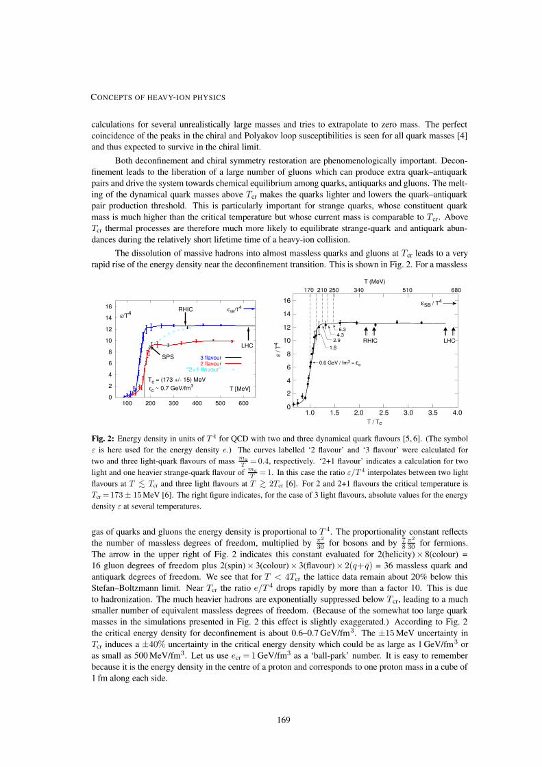
The dissolution of massive hadrons into almost massless quarks and gluons at Tcr leads to a very

rapid rise of the energy density near the deconfinement transition. This is shown in Fig. 2. For a massless

0

2

4

6

8

10

12

14

16

100 200 300 400 500 600

T [MeV]

ε/T4εSB/T4

Tc = (173 +/- 15) MeVεc ~ 0.7 GeV/fm3

RHIC

LHC

SPS 3 flavour2 flavour

‘‘2+1-flavour’’

170

16

14

12

10

8

6

4

2

01.0 1.5 2.0 2.5 3.0 3.5 4.0

210 250 340 510

LHCRHIC

680

εSB / T4

T / Tc

T (MeV)ε

/T4

6.34.3

2.91.8

0.6 GeV / fm3 = εc

Fig. 2: Energy density in units of T 4 for QCD with two and three dynamical quark flavours [5, 6]. (The symbol

ε is here used for the energy density e.) The curves labelled ‘2 flavour’ and ‘3 flavour’ were calculated for

two and three light-quark flavours of massmq

T = 0.4, respectively. ‘2+1 flavour’ indicates a calculation for two

light and one heavier strange-quark flavour ofmq

T = 1. In this case the ratio ε/T 4 interpolates between two light

flavours at T . Tcr and three light flavours at T & 2Tcr [6]. For 2 and 2+1 flavours the critical temperature is

Tcr =173 ± 15 MeV [6]. The right figure indicates, for the case of 3 light flavours, absolute values for the energy

density ε at several temperatures.

gas of quarks and gluons the energy density is proportional to T 4. The proportionality constant reflects

the number of massless degrees of freedom, multiplied by π2

30 for bosons and by 78π2

30 for fermions.

The arrow in the upper right of Fig. 2 indicates this constant evaluated for 2(helicity)× 8(colour) =

16 gluon degrees of freedom plus 2(spin)× 3(colour)× 3(flavour)× 2(q+ q) = 36 massless quark and

antiquark degrees of freedom. We see that for T < 4Tcr the lattice data remain about 20% below this

Stefan–Boltzmann limit. Near Tcr the ratio e/T 4 drops rapidly by more than a factor 10. This is due

to hadronization. The much heavier hadrons are exponentially suppressed below Tcr, leading to a much

smaller number of equivalent massless degrees of freedom. (Because of the somewhat too large quark

masses in the simulations presented in Fig. 2 this effect is slightly exaggerated.) According to Fig. 2

the critical energy density for deconfinement is about 0.6–0.7 GeV/fm3. The ±15 MeV uncertainty in

Tcr induces a ±40% uncertainty in the critical energy density which could be as large as 1 GeV/fm3 or

as small as 500 MeV/fm3. Let us use ecr = 1 GeV/fm3 as a ‘ball-park’ number. It is easy to remember

because it is the energy density in the centre of a proton and corresponds to one proton mass in a cube of

1 fm along each side.


169

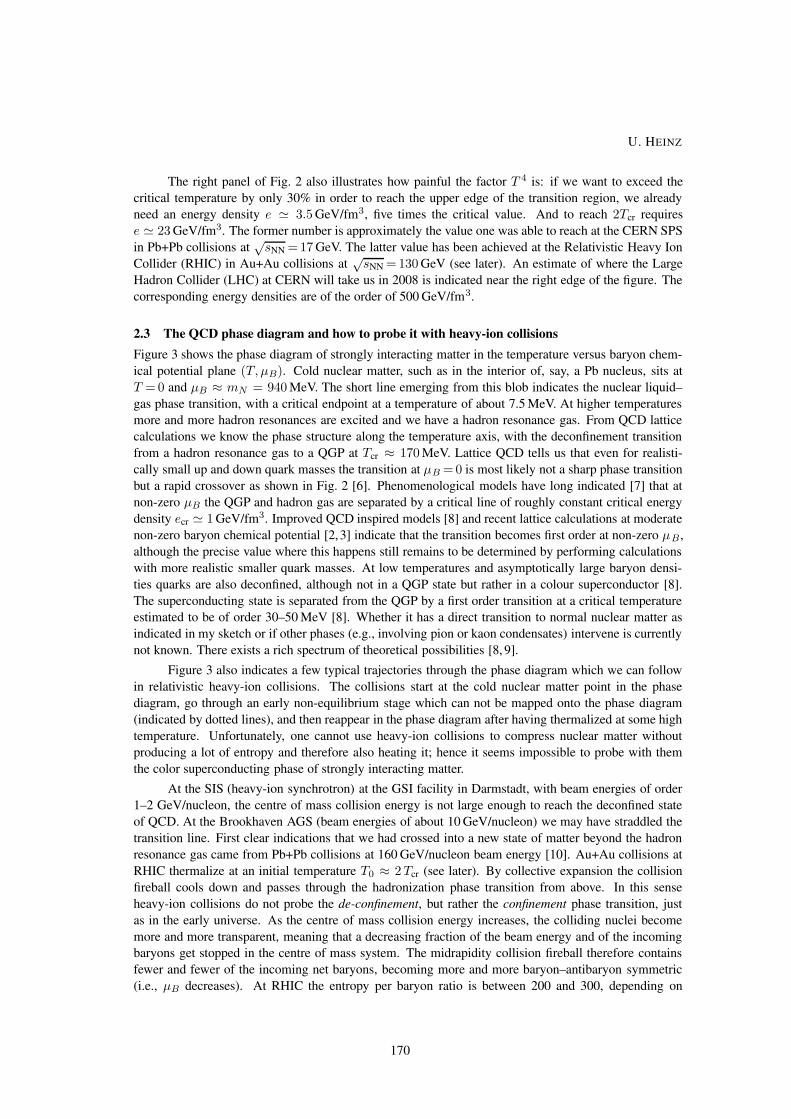
The right panel of Fig. 2 also illustrates how painful the factor T 4 is: if we want to exceed the

critical temperature by only 30% in order to reach the upper edge of the transition region, we already

need an energy density e ' 3.5 GeV/fm3, five times the critical value. And to reach 2Tcr requires

e ' 23 GeV/fm3. The former number is approximately the value one was able to reach at the CERN SPS

in Pb+Pb collisions at√sNN =17 GeV. The latter value has been achieved at the Relativistic Heavy Ion

Collider (RHIC) in Au+Au collisions at√sNN = 130 GeV (see later). An estimate of where the Large

Hadron Collider (LHC) at CERN will take us in 2008 is indicated near the right edge of the figure. The

corresponding energy densities are of the order of 500 GeV/fm3.

2.3 The QCD phase diagram and how to probe it with heavy-ion collisions

Figure 3 shows the phase diagram of strongly interacting matter in the temperature versus baryon chem-

ical potential plane (T, µB). Cold nuclear matter, such as in the interior of, say, a Pb nucleus, sits at

T = 0 and µB ≈ mN = 940 MeV. The short line emerging from this blob indicates the nuclear liquid–

gas phase transition, with a critical endpoint at a temperature of about 7.5 MeV. At higher temperatures

more and more hadron resonances are excited and we have a hadron resonance gas. From QCD lattice

calculations we know the phase structure along the temperature axis, with the deconfinement transition

from a hadron resonance gas to a QGP at Tcr ≈ 170 MeV. Lattice QCD tells us that even for realisti-

cally small up and down quark masses the transition at µB = 0 is most likely not a sharp phase transition

but a rapid crossover as shown in Fig. 2 [6]. Phenomenological models have long indicated [7] that at

non-zero µB the QGP and hadron gas are separated by a critical line of roughly constant critical energy

density ecr ' 1 GeV/fm3. Improved QCD inspired models [8] and recent lattice calculations at moderate

non-zero baryon chemical potential [2,3] indicate that the transition becomes first order at non-zero µB ,

although the precise value where this happens still remains to be determined by performing calculations

with more realistic smaller quark masses. At low temperatures and asymptotically large baryon densi-

ties quarks are also deconfined, although not in a QGP state but rather in a colour superconductor [8].

The superconducting state is separated from the QGP by a first order transition at a critical temperature

estimated to be of order 30–50 MeV [8]. Whether it has a direct transition to normal nuclear matter as

indicated in my sketch or if other phases (e.g., involving pion or kaon condensates) intervene is currently

not known. There exists a rich spectrum of theoretical possibilities [8, 9].

Figure 3 also indicates a few typical trajectories through the phase diagram which we can follow

in relativistic heavy-ion collisions. The collisions start at the cold nuclear matter point in the phase

diagram, go through an early non-equilibrium stage which can not be mapped onto the phase diagram

(indicated by dotted lines), and then reappear in the phase diagram after having thermalized at some high

temperature. Unfortunately, one cannot use heavy-ion collisions to compress nuclear matter without

producing a lot of entropy and therefore also heating it; hence it seems impossible to probe with them

the color superconducting phase of strongly interacting matter.

At the SIS (heavy-ion synchrotron) at the GSI facility in Darmstadt, with beam energies of order

1–2 GeV/nucleon, the centre of mass collision energy is not large enough to reach the deconfined state

of QCD. At the Brookhaven AGS (beam energies of about 10 GeV/nucleon) we may have straddled the

transition line. First clear indications that we had crossed into a new state of matter beyond the hadron

resonance gas came from Pb+Pb collisions at 160 GeV/nucleon beam energy [10]. Au+Au collisions at

RHIC thermalize at an initial temperature T0 ≈ 2Tcr (see later). By collective expansion the collision

fireball cools down and passes through the hadronization phase transition from above. In this sense

heavy-ion collisions do not probe the de-confinement, but rather the confinement phase transition, just

as in the early universe. As the centre of mass collision energy increases, the colliding nuclei become

more and more transparent, meaning that a decreasing fraction of the beam energy and of the incoming

baryons get stopped in the centre of mass system. The midrapidity collision fireball therefore contains

fewer and fewer of the incoming net baryons, becoming more and more baryon–antibaryon symmetric

(i.e., µB decreases). At RHIC the entropy per baryon ratio is between 200 and 300, depending on

U. HEINZ

170

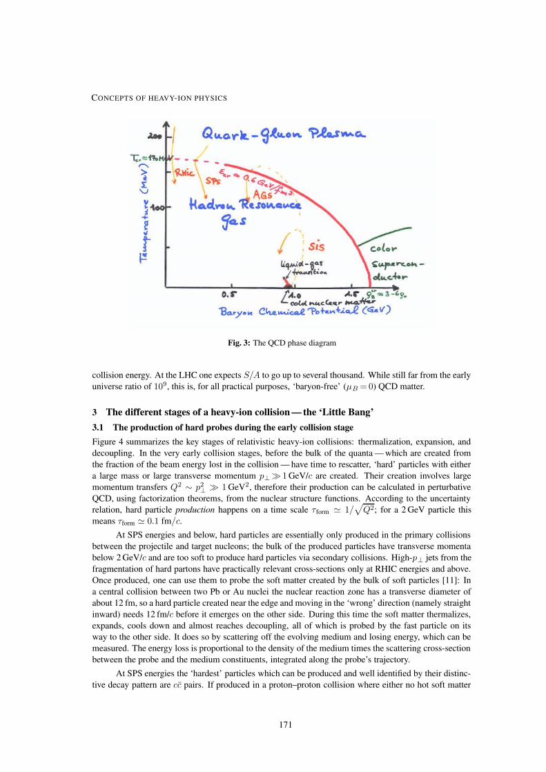
Fig. 3: The QCD phase diagram

collision energy. At the LHC one expects S/A to go up to several thousand. While still far from the early

universe ratio of 109, this is, for all practical purposes, ‘baryon-free’ (µB = 0) QCD matter.

3 The different stages of a heavy-ion collision — the ‘Little Bang’

3.1 The production of hard probes during the early collision stage

Figure 4 summarizes the key stages of relativistic heavy-ion collisions: thermalization, expansion, and

decoupling. In the very early collision stages, before the bulk of the quanta — which are created from

the fraction of the beam energy lost in the collision — have time to rescatter, ‘hard’ particles with either

a large mass or large transverse momentum p⊥ 1 GeV/c are created. Their creation involves large

momentum transfers Q2 ∼ p2⊥ 1 GeV2, therefore their production can be calculated in perturbative

QCD, using factorization theorems, from the nuclear structure functions. According to the uncertainty

relation, hard particle production happens on a time scale τform ' 1/√Q2; for a 2 GeV particle this

means τform ' 0.1 fm/c.

At SPS energies and below, hard particles are essentially only produced in the primary collisions

between the projectile and target nucleons; the bulk of the produced particles have transverse momenta

below 2 GeV/c and are too soft to produce hard particles via secondary collisions. High-p⊥ jets from the

fragmentation of hard partons have practically relevant cross-sections only at RHIC energies and above.

Once produced, one can use them to probe the soft matter created by the bulk of soft particles [11]: In

a central collision between two Pb or Au nuclei the nuclear reaction zone has a transverse diameter of

about 12 fm, so a hard particle created near the edge and moving in the ‘wrong’ direction (namely straight

inward) needs 12 fm/c before it emerges on the other side. During this time the soft matter thermalizes,

expands, cools down and almost reaches decoupling, all of which is probed by the fast particle on its

way to the other side. It does so by scattering off the evolving medium and losing energy, which can be

measured. The energy loss is proportional to the density of the medium times the scattering cross-section

between the probe and the medium constituents, integrated along the probe’s trajectory.

At SPS energies the ‘hardest’ particles which can be produced and well identified by their distinc-

tive decay pattern are cc pairs. If produced in a proton–proton collision where either no hot soft matter


171

Fig. 4: Stages of a relativistic heavy-ion collision and relevant theoretical concepts

is created or the charmed quarks leave the region in which soft particles are formed before that happens,

these charmed quarks and antiquarks form either a bound charmonium state (J/ψ, ψ ′, or χ, ‘hidden

charm’ production) or they find light quark partners to hadronize into ‘open charm’ states (D and Dmesons or charmed baryons). The corresponding branching ratios are well-known — the hidden charm

states form a very small fraction (less than 1%) of all final states. If the cc pair is created in a heavy-ion

collision, something similar to the jets discussed above happens: the two heavy quarks have to travel

through a dense medium of soft particles, which interferes with their intention to hadronize and modifies

their branching ratios into open and hidden charm states. In particular, if the soft medium thermalizes

into a QGP, the colour interaction between the c and c is Debye screened by the coloured quarks and

gluons in the plasma, thereby prohibiting their normal binding into one of the charmonium states. This

should cause ‘J/ψ suppression’ [12].

Other probes of the early collision stage are direct photons [13], either real or virtual, in which

case they materialize as lepton–antilepton (e+e− or µ+µ−) pairs, generally known as ‘dileptons’. Such

photons are produced by the electric charges in the medium (i.e., by quarks and antiquarks during the

early collision stage). Their production cross-section is proportional to the square of the Sommerfeld

U. HEINZ

172

fine structure constant α= 1137 and thus small, but since they also reinteract only with this small electro-

magnetic cross-section their mean free path even in a very dense QGP is of the order of 50 000 fm and

thus much larger than any conceivable heavy-ion fireball. In contrast to all hadronic probes, they thus

escape from the collision zone without reinteraction and carry pristine information about the momentum

distributions of their parent quarks and antiquarks into the detector. Real and virtual photons are emit-

ted throughout the collision and expansion stage, and their measured spectrum thus integrates over the

expansion history of the collision fireball. However, their production rate from a thermal system scales

with a high power of the temperature (∼T 4 in a static heat bath but ∼T 6 once the effects of expansion

are taken into account [13]) and is thus strongly biased towards the early collision stages. Unfortunately,

the directly emitted photons and dileptons must be dug out from a huge background of indirect pho-

tons and a large combinatorial background of uncorrelated lepton pairs resulting from electromagnetic

and weak decays of hadrons after hadronic freeze-out. This renders the measurement of these clean

electromagnetic signals difficult.

3.2 Thermalization and expansion

The key difference between elementary particle and nucleus–nucleus collisions is that the quanta created

in the primary collisions between the incoming nucleons can not immediately escape into the surrounding

vacuum, but rescatter off each other. In this way they create a form of dense, strongly interacting matter

which, when it thermalizes quickly enough and at sufficiently large energy density, is a QGP. This is why

with heavy-ion collisions we have a chance to recreate the matter in the very early universe, whereas

with high-energy collisions between leptons or single hadrons we do not.

The produced partons rescatter both elastically and inelastically. Both types of collision lead to

equipartitioning of the deposited energy, but only the inelastic collisions change the relative abundances

of gluons, light quarks and strange quarks. [To also change the abundance of the heavier charm quarks

(mc ' 1200 MeV) requires secondary collisions of sufficient energy, which do not happen at the SPS but

may play a role at RHIC and above.] From the phenomenology of pp collisions it is known [14, 15] that

the produced hadron abundances are distributed statistically, but that strange hadrons are systematically

suppressed (probably because strange quarks are not present in the initial state and their large constituent

mass of ' 450 MeV makes them hard to create from the vacuum as the produced partons hadronize).

In a heavy-ion collision, if the reaction zone thermalizes at energy density >ecr such that gluons are

deconfined and chiral symmetry is restored, strange quarks are much lighter (ms' 150 MeV) and can

be relatively easily created by secondary collisions among the many gluons, leading to chemical equi-

libration between light and strange quarks [16]. The observed strangeness suppression in pp collisions

should thus be reduced or absent in relativistic heavy-ion collisions [17].

A thermalized system has thermal pressure which, when acting against the surrounding vacuum,

leads to collective (hydrodynamic) expansion of the collision fireball. As a consequence, the fireball

cools and its energy density decreases. When the latter reaches ecr ' 1 GeV/fm3, the partons convert to

hadrons. During this phase transition the entropy density drops steeply over a small temperature interval

(similar to the energy density shown in Fig. 2). Since the total entropy cannot decrease this implies

that the fireball volume must increase by a large factor while the temperature remains approximately

constant. The growth of the fireball volume takes time, so the fireball ends up spending significant

time near Tcr. Furthermore, while the matter hadronizes its speed of sound cs =√∂p/∂e is small [6],

causing inefficient acceleration so that the collective flow does not increase during this period. This

may be visible in the direct photon spectrum: an inverse Laplace transform should show a particularly

strong weight at the transition temperature, blueshifted by the prevailing radial flow as the system crosses

Tcr [18]. The softness of the equation of state near the phase transition should also manifest itself in the

centre-of-mass energy dependence of the collective flow, as discussed later.


173

3.3 Hadronic freeze-out and post-freeze-out decays

After hadronization of the fireball, the hadrons keep rescattering with each other for a while, continuing

to build up expansion flow, until the matter becomes so dilute that the average distance between hadrons

exceeds the range of the strong interactions. At this point all scattering stops and the hadrons decouple

(‘freeze out’). Actually, their abundances already freeze out earlier when the rates for inelastic processes,

in which the hadrons change their identity, become too small to keep up with the expansion. Since the

corresponding inelastic cross-sections are only a small fraction of the total cross-section, inelastic pro-

cesses stop long before the elastic ones, leading to earlier freeze-out for the hadron abundances than for

their momenta: chemical freeze-out precedes thermal or kinetic freeze-out. What I call ‘elastic’ includes

resonant processes such as π+N → ∆ → π+N where two hadrons form a short-lived resonance which

subsequently decays back into the same particles (possible with different electric charge assignments).

Such processes do not change the finally observed chemical composition, but they contribute to the ther-

malization of the momenta and have large ‘resonant’ cross-sections. Since most of the hadrons in a

relativistic heavy-ion fireball are pions (since they are so light), resonances with pions are very efficient

in keeping the system in thermal equilibrium (even after chemical equilibrium has been broken). For

scattering among pions the ρ resonance plays a large role while kaons and (anti)baryons couple to the

pion fluid via the K∗, ∆ and Y ∗ resonances. Because of the particularly large ∆ and Y ∗ resonance

cross-sections, even at RHIC and LHC (where the net baryon density is small) baryon–antibaryon pairs

play an important role as part of the ‘glue’ that keeps the expanding pion fluid thermalized well below

the chemical freeze-out point.

At kinetic freeze-out all hadrons, including the then present unstable resonances, have an approxi-

mately exponential transverse momentum spectrum reflecting the temperature of the fireball at that point,

blueshifted by the average transverse collective flow. The unstable resonances decay, however, producing

daughter particles with, on average, smaller transverse momenta. The experimentally measured spectra

of stable hadrons cannot be understood without adding these decay products to the originally emitted

spectra. Since most resonances decay by emitting a pion, this effect is particularly important for the pion

spectrum which at low p⊥ is completely dominated by decay products. This seriously affects the slope

of their spectrum out to p⊥' 700 MeV [19,20], making it steeper than the blueshifted thermal spectrum

of the directly emitted hadrons.

3.4 Theoretical tools

The idea that the parton production process factorizes into a perturbatively calculable ‘hard’ QCD cross-

section and a non-perturbative, experimentally determined nuclear parton structure function (or parton

distribution function) can be used to describe the initial production of hard partons, with pT >p0 where

p0 & 1−2 GeV describes the lower applicability limit of this type of approach [21, 22]. The production

of soft partons is usually non-perturbative and requires phenomenological models, such as string mod-

els [23], for their description. At very high collision energies particle production at midrapidity (i.e.,

particles with small longitudinal momenta in the centre-of-momentum frame) probes the nuclear struc-

ture functions at small x where x is the fraction of the beam momentum carried by the partons whose

collision produces the secondary partons. At small x the gluon distribution function becomes very big

and gluons begin to fill the transverse area of the colliding nuclei densely [24, 25]. The gluons start to

recombine, leading to gluon saturation, and low-pT gluon modes are occupied by a macroscopic number

of gluons ∼ 1/αs where the effective strong coupling αs is small because of the high density of glu-

ons [26]. As a result, the initial gluons can be effectively described by a classical gluon field [26, 27] in

which the coupling is weak but nonlinear density effects are important (this state has become known as

the ‘colour glass condensate’ [28]). The production of soft secondary gluons can be understood as the

liberation of these gluons by breaking the coherence of their multiparticle wavefunction [27, 29]. The

collision energies where these modern ideas become applicable lie probably beyond the RHIC range, but

this is an exciting and active field of ongoing research which may come to fruition at the LHC.

U. HEINZ

174

After the initial parton production or ‘liberation’ process one must describe the rescattering and

thermalization of the produced quanta. For not too dense systems this can be done with classical kinetic

transport theory (relativistic Boltzmann equation), also known as parton cascade [30, 31]. In the early

collision stages at RHIC and LHC energies the densities are probably too high for this to remain a

reliable approach, and one must switch to quantum transport theory [32]. This formalism has not yet been

developed very well for practical applications, and much interesting work is going on in this direction

(eg., Refs. [33,34]). None of these approaches, which usually invoke perturbative QCD arguments to

describe the microscopic scattering processes, has so far been able to produce parton thermalization

time scales at RHIC which are shorter than about 5 fm/c [33]. This is too long for heavy-ion collisions

whose typical expansion time scale (Hubble time) is only a couple of fm/c. As I will show later there is

strong phenomenological evidence that thermalization must happen much more quickly. This presents

an interesting challenge for theory and indicates the importance of strong non-perturbative effects in the

early collision stages and the QGP.

Once local thermal equilibrium has been reached, the further evolution can be described hydrody-

namically. The simplest version of such an approach is ideal fluid dynamics, which will be discussed in

more detail later. The fireball can be described as an ideal fluid if the microscopic scattering time scale

is much shorter than any macroscopic time scale associated with the fireball evolution. If this is not the

case, one should include non-ideal effects such as shear, diffusion and heat conduction. This requires the

calculation of the corresponding transport coefficients in a partonic system close to thermal equilibrium.

Much work is going on in this direction (see e.g., Refs. [35–37]), but systematic approaches based on

perturbatively resummed thermal QCD [35–37] give phenomenologically unacceptably large values for

these transport coefficients, again indicating the importance of non-perturbative effects.

The hydrodynamic equations require knowledge of the equation of state, i.e., the relationship

p(e, nB) between the pressure, energy density and baryon density. For small nB this is known from

lattice QCD; for large nB one extrapolates the lattice results with phenomenological models (see Ref.

[9] for a recent review). Hydrodynamics is the ideal language for relating observed collective flow

phenomena to the equation of state. Since it only requires the equation of state but no detailed knowledge

of the microscopic collision dynamics, it permits an easy description of the hadronization phase transition

without any need for a microscopic understanding of how hadrons form from quarks and gluons. Of

course, the underlying assumption is that all these microscopic processes happen so fast that the system

never strays appreciably from a local thermal equilibrium.

After hadronization the system continues to expand and dilute until the average distance between

hadrons becomes larger than the range of the strong interaction. At this point the hadrons decouple, i.e.,

their momenta stop changing until they are recorded by the detector. One can implement this decoupling

or ‘kinetic freeze-out’ in different ways, either by truncating the hydrodynamic phase abruptly with the

Cooper–Frye algorithm (see below) or by switching back from hydrodynamics to a (this time hadronic)

cascade [38–40] in which decoupling happens automatically and selfconsistently. In the Cooper–Frye

algorithm one also must take into account that in this approach all kinds of hadrons decouple simulta-

neously, and that unstable hadron resonances decay subsequently by strong (and in some situations also

by weak) interactions before their stable daughter products reach the detector. To compute the measured

spectra one must therefore fold the initially emitted Cooper–Frye hadron spectra with these decays [19].

Some studies, such as two-particle momentum correlations, also require the computation of long-range

final state interaction effects, such as the Coulomb repulsion/attraction between charged hadrons which

continues long after their strong interactions with each other have ceased.

3.5 Strategies for reconstructing the Little Bang

The bulk (over 99%) of the particles produced in heavy-ion collisions are hadrons. These are strongly

interacting particles which cannot decouple from the fireball before the system is so dilute that strong

interactions cease. Their observed momenta thus provide a snapshot of the kinetic decoupling stage


175

(‘thermal freeze-out’). In this sense hadrons are the Little Bang analogue of the cosmic microwave back-

ground in the Big Bang. As discussed in Section 3.3, hadron abundances freeze out earlier. As we will

see later, this ‘chemical freeze-out’ happens right after hadronization, i.e., the finally observed hadron

abundances are generated by the hadronization process itself. This primordial hadrosynthesis is the Lit-

tle Bang analogue of primordial nucleosynthesis in the Big Bang. As the hadrons decouple, they carry

not only thermal information about the prevalent temperature at chemical and thermal freeze-out, but in

the momentum spectra this information is folded with (i.e., blueshifted by) the collective expansion flow,

just as the temperature of the cosmic microwave radiation is redshifted by the cosmological expansion.

The hydrodynamic expansion flow is the Little Bang analogue of the cosmic Hubble expansion in the

Big Bang. (Of course, the origin of the expansion is entirely different in the two cases: in heavy-ion

collisions it is generated hydrodynamically by pressure gradients whereas in the Big Bang it reflects an

initial condition, modified over billions of years by the effects of the gravitational interaction. But the

velocity profiles turn out to be surprisingly similar, as we will see!)

We reconstruct the Little Bang from these ‘late’ hadronic observables very much like we recon-

structed the Big Bang from the three pillars of cosmology: Hubble expansion, CMB, and primordial

nuclear abundances. The hadronic observables are abundant and can be measured with high statistical

accuracy. As I will show, their theoretical analysis allows us to separate the thermal from the collective

motion. The collective flow provides a memory of the pressure and other thermodynamic conditions

during the earlier collision stages. In fact, we will see that certain anisotropies in the flow patterns seen

in non-central heavy-ion collisions (‘elliptic flow’) provide a unique window into the very early collision

stages and are no longer changed after about 5 fm/c after initial impact. As you will see, a (in my opin-

ion) watertight proof for thermalization during this early stage, at a time τ therm < 1 fm/c and at prevalent

energy densities which exceed the critical value ecr for deconfinement by at least an order of magnitude,

can be based on the accurately measured elliptic flow of the final state hadrons. (This is a bit analogous

to the indelible imprint that cosmic inflation has left on the density fluctuations in the universe, which can

be accurately measured through the anisotropy of the cosmic microwave radiation which only decoupled

300 000 years later.)

The reconstruction of the global space-time evolution of the reaction zone from the finally ob-

served soft hadrons is the cornerstone of the program. The reconstructed dynamical picture will be the

basis on which other rarer observables, in particular the ‘deep’ or ‘hard’ probes, will be interpreted. For

example, jet quenching and heavy quarkonium suppression cannot be quantitatively interpreted without

knowledge of the fireball density and its space-time evolution, and direct photon and dilepton spectra

cannot be properly understood without a relatively accurate idea about the transverse flow patterns at the

time of photon emission. Still, these probes will in the end be the only direct access we will ever have to

the temperature and energy density at the beginning of the expansion when the system was a QGP, and

although they cannot be fully interpreted and exploited without the later emitted soft particles they are

still an indispensable part of the picture. This illustrates the network-like interdependence between soft

and hard observables in their role for elucidating heavy-ion collision and QGP dynamics.

4 The Little Bang — collective explosion of a thermalized system

An unavoidable consequence of QGP formation in heavy-ion collisions is collective flow. Since a QGP

is by definition an (approximately) thermalized system of quarks and gluons, it has thermal pressure, and

the pressure gradients with respect to the surrounding vacuum cause the QGP to explode. Absence of

collective flow would indicate absence of pressure and imply absence of a hot thermalized system and, a

fortiori, of a QGP.

In this chapter we will therefore do two things: (i) learn how to analyse the measured particle

spectra for the presence of collective flow and how to separate it from random thermal motion, and (ii)

compute the expected collective flow patterns from reasonable initial conditions using a hydrodynamic

model. By comparing with experiments we can fine-tune the initial conditions, learn about the equation

U. HEINZ

176

of state of the hot expanding matter and, most importantly, find out about when and at which energy

densities the thermal pressure builds up and begins to drive the collective expansion.

4.1 Radial flow

4.1.1 Flow defined

Consider a nuclear fireball undergoing collective expansion. Collective flow is defined by the following

operational procedure: at any space-time point x in the fireball, we consider an infinitesimal volume ele-

ment centered at that point and add up all the four-momenta of the quanta in it. The total three-momentum

P obtained in this way, divided by the associated total energy P 0, defines the average ‘flow’ velocity

v(x) of the matter at point x through the relation P /P 0 = v. Collective flow thus describes a correlation

between the average momentum of the particles and their space–time position, a so-called x-p correla-

tion. With v(x) we can associate a normalized four-velocity uµ = γ(1,v) where γ(x)= 1/√

1−v2(x)is the corresponding Lorentz dilation factor and u·u=uµuµ = 1 (in units where the speed of light c= 1).

I separate the flow velocity v(x) into its components along the beam direction (‘longitudinal flow’

vL) and in the plane perpendicular to the beam (‘transverse plane’) which I call ‘transverse flow’ v⊥. The

magnitude v⊥ may depend on the azimuthal angle around the beam direction, i.e., on the angle between

v⊥ and the impact parameter b of the collision. In this case we call the transverse flow ‘anisotropic’. Its

azimuthal average we call radial flow.

4.1.2 Local thermodynamic equilibrium

If the fireball is in local thermodynamic equilibrium, we can not only define a local flow four-velocity

uµ(x), but also a local temperature T (x) and, for each particle species i, a chemical potential µ i(x)which controls its particle density at point x. In this case the phase-space distribution of particles of type

i is given by the Lorentz covariant local equilibrium distribution

fi,eq(x, p) =gi

e[p·u(x)−µi(x)]/T (x) ± 1= gi

∞∑

n=1

(∓)n+1 e−n[p·u(x)−µi(x)]/T (x) . (10)

Here gi is a spin–isospin–colour–flavour–etc., degeneracy factor which counts all particles with the same

mass mi and chemical potential µi. The factor p ·u(x) in the exponent is the energy of the particle in the

local rest frame (local heat bath frame), boosted to the observer frame by the flow four-velocity uµ(x)of the fluid cell at point x (p · u→ p0 =E when uµ→ (1,0)). The ±1 in the denominator accounts

for the proper quantum statistics of particle species i (upper sign for fermions, lower sign for bosons).

The Boltzmann approximation corresponds to keeping only the first term in the sum over n in the last

expression. In our applications this is an excellent analytical approximation for all hadrons except for

the pion. Pions and quarks and gluons are too light, mi . T , and one must use the proper quantum

statistical distributions.

4.1.3 Rapidity coordinates

At relativistic energies it is convenient to parametrize the longitudinal flow velocities and momenta in

terms of rapidities (for any velocity v the associated rapidity is η= 12 ln 1+v

1−v or v= tanh η):

ηL =1

2ln

1+vL

1−vL

, y =1

2ln

1+pL

E

1−pL

E

=1

2lnE+pL

E−pL

. (11)

As vL → 1, we have that ηL →∞. Rapidities have the advantage over longitudinal velocities that they are

additive under longitudinal boosts: a fluid cell with flow rapidity ηL in a given inertial frame has rapidity


177

η′L = ηL + ∆η in another inertial frame which moves relative to the first frame with rapidity ∆η in the

−z direction. The flow four-vector (u0,u)= (u0,u⊥, uL) is then parametrized as

uµ = γ⊥(cosh ηL, vx, vy, sinh ηL

)with γ⊥ =

1√1−v2

⊥

=1√

1−v2x−v2

y

(12)

where v⊥ = (vx, vy) is the transverse flow velocity. Similarly the four-momentum pµ =(E,p⊥, pL) is

written as

pµ =(m⊥ cosh y, px, py, m⊥ sinh y

)with m⊥ =

√m2+p2

⊥ =√m2+p2

x+p2y (13)

which obviously satisfies the mass-shell constraint p2 = pµpµ=m2. [We use the notations p⊥ and pT

interchangeably for the transverse momentum, and similarly mT and m⊥ for the ‘transverse mass’ — in

the literature one often also finds the notations pt and mt.] The scalar product p · u(x) in the exponent of

the Boltzmann factor then becomes

p · u = γ⊥(m⊥ cosh(y−ηL) − v⊥ · p⊥

). (14)

4.1.4 Longitudinal boost-invariance and Bjorken scaling

So far no approximations have been made as long as we allow v⊥ and ηL to be arbitrary functions of

xµ = (t, r⊥, z) where r⊥ = (x, y) denotes the transverse coordinates. Things simplify, however, enor-

mously if one assumes longitudinal boost-invariance. Bjorken [41] argued that at asymptotically high

energies the physics of secondary particle production should be independent of the longitudinal reference

frame. This condition can be easily expressed if one puts the nuclear collision at longitudinal position

z= 0 and introduces, instead of z and t, the following ‘space-time rapidity’ and ‘longitudinal proper

time’ coordinates to describe the forward light cone emanating from the collision point:

η =1

2lnt+z

t−z =1

2ln

1+ zt

1− zt

, τ =√t2−z2 . (15)

In these coordinates xµ = (t, r⊥, z) reads xµ = (τ cosh η, r⊥, τ sinh η), and the space-time integration

measure takes the form d4x= τ dτ dη d2r⊥. In a t-z diagram, lines of constant space-time rapidity

are rays through the origin with slope 1/ tanh η. Longitudinal boost-invariance of particle production

then implies that the initial conditions for local observables (such as particle and energy densities) are

only functions of τ and r⊥, but independent of η [41]. Furthermore, the boost-invariance of these

initial conditions is preserved in longitudinal proper time if the system expands collectively along the

longitudinal direction with a very specific ‘scaling’ velocity profile vL = zt [41]. Inserting this into the

definition (11) for the longitudinal fluid rapidity ηL and comparing with (15), we see that longitudinal

boost-invariance implies the identity

ηL = η (Bjorken scaling) (16)

of the longitudinal fluid rapidity with the space-time rapidity. Since ηL(x) characterizes the average

longitudinal momentum of the produced particles at point x whereas η characterizes the coordinate xitself, this identity implies a very strong correlation between the average longitudinal momentum and the

longitudinal position.

The Bjorken scaling approximation is expected to be good at high energies and not too close to

the beam and target rapidities, i.e., a safe distance from the longitudinal kinematic limits. We will use

it to describe particle production near midrapidity (y ≈ 0 in the centre-of-mass frame). As a result of

Bjorken scaling, the Boltzmann exponent reduces to

p · u(x) = γ⊥(r⊥, τ)(m⊥ cosh(y−η) − p⊥ · v⊥(r⊥, τ)

). (17)

U. HEINZ

178

Owing to the additivity of rapidities, this is manifestly invariant under longitudinal boosts since it only

involves rapidity differences. The transverse flow velocity, as well as the temperature T and chemical

potential µi, are independent of η and depend only on the transverse position r⊥ and longitudinal proper

time τ .

4.1.5 The Cooper–Frye formula

Suppose we want to count the total number of particles of species i produced in the collision. Since

this number does not depend on the reference frame of the observer, we must be able to express it in a

Lorentz-invariant way. We define a three-dimensional hypersurface Σ(x) in four-dimensional space–time

along which we perform the counting. The simplest case would be a measurement in all space at a fixed

global time t. In a space-time diagram this would correspond to a horizontal line at fixed t. But this is not

how a real detector works. In an ideal detector, we surround the collision region hermetically by detector

elements which sit stationary at a fixed distance from the collision point, and we wait until the particles

pass through these detector elements (which particles with different velocities will do at different times).

Assuming, for example, a spherical detector of radiusR, the corresponding detection hypersurface would

in a (t, r) space-time diagram be represented by a vertical line at fixed r=R, extending from t=−∞ to

t=∞. In this case the hypersurface is a two-dimensional sphere extending over all time, i.e. it is again

three-dimensional.

You see that different choices for the three-dimensional hypersurface Σ are possible as long as it

completely closes off the future light cone emerging from the collision point. We count particles crossing

the surface by subdividing it into infinitesimal elements d3σ, defining an outward-pointing four-vector

d3σµ(x) perpendicular to Σ(x) at point x with the magnitude d3σ, computing the scalar product of

the four-vector jµi (x) describing the current of particles i through point x, and summing over all such

infinitesimal hypersurface elements:

Ni =

∫

Σd3σµ(x) j

µi (x) =

∫

Σd3σµ(x)

(1

(2π)3

∫d3p

Epµ fi(x, p)

). (18)

The particle number current density jµi (x) is given in terms of the Lorentz-invariant phase-space distri-

bution (giving the probability of finding a particle with momentum p at point x) by multiplying it with the

velocitypµ

E and integrating over all momenta with measured3ph3 = d3p

(2π~)3 where h= 2π~ = 2π is Planck’s

quantum of action and we are using units where ~ = 1.

Dividing by the Lorentz-invariant momentum-space measure d3pE (which in rapidity coordinates

reads dy p⊥dp⊥ dϕp = dym⊥dm⊥ dϕp where ϕp is the azimuthal angle of p⊥) we obtain the invariant

momentum distribution for particle species i:

EdNi

d3p=

dNi

dy p⊥dp⊥ dϕp=

dNi

dy m⊥dm⊥ dϕp=

1

(2π)3

∫

Σp · d3σµ(x) fi(x, p) . (19)

This is the Cooper–Frye formula [42]. One can show that two different surfaces Σ1 and Σ2 give the

same particle number Ni if between Σ1 and Σ2 the distribution function fi(x, p) evolves via a Boltzmann

equation with a collision kernel which preserves the number of particles i, and that we obtain the same

momentum spectrum if and only if fi(x, p) evolves from Σ1 to Σ2 by free-streaming, i.e., if fi is a

solution of the collisionless Boltzmann equation. To compute the measured momentum spectrum we

can therefore replace the surface Σ corresponding to the detector by shrinking it to the smallest and

earliest surface that still encloses all scattering processes. We call this the ‘surface of last scattering’ or

‘freeze-out surface’ Σf.


179

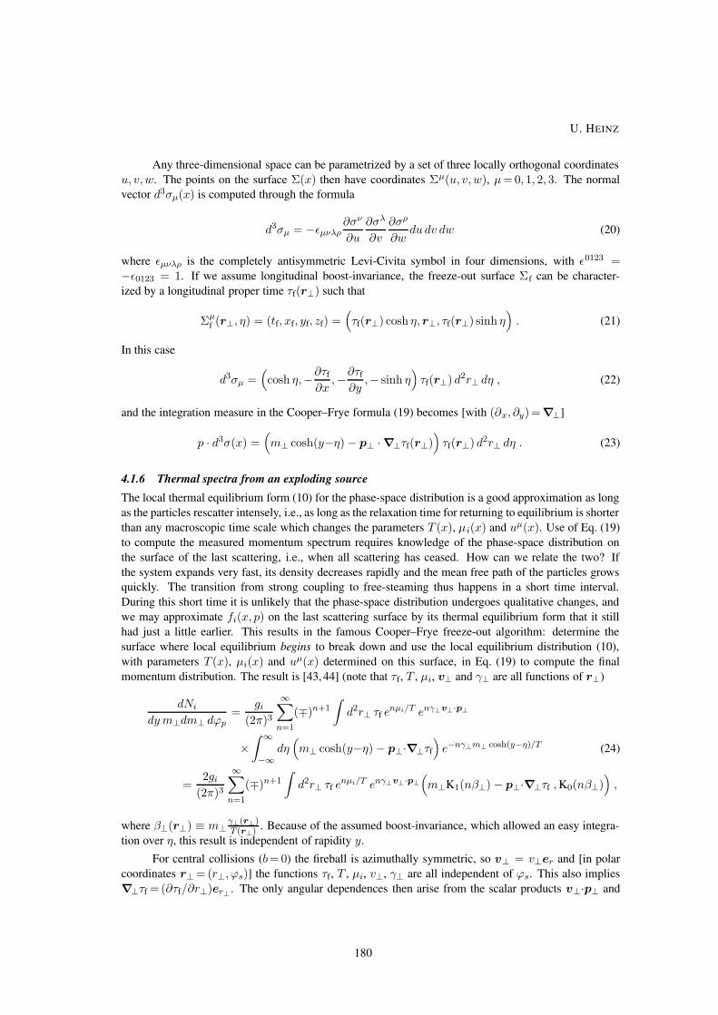
Any three-dimensional space can be parametrized by a set of three locally orthogonal coordinates

u, v,w. The points on the surface Σ(x) then have coordinates Σµ(u, v,w), µ= 0, 1, 2, 3. The normal

vector d3σµ(x) is computed through the formula

d3σµ = −εµνλρ∂σν

∂u

∂σλ

∂v

∂σρ

∂wdu dv dw (20)

where εµνλρ is the completely antisymmetric Levi-Civita symbol in four dimensions, with ε0123 =−ε0123 = 1. If we assume longitudinal boost-invariance, the freeze-out surface Σf can be character-

ized by a longitudinal proper time τf(r⊥) such that

Σµf (r⊥, η) = (tf, xf, yf, zf) =

(τf(r⊥) cosh η, r⊥, τf(r⊥) sinh η

). (21)

In this case

d3σµ =(cosh η,−∂τf

∂x,−∂τf

∂y,− sinh η

)τf(r⊥) d2r⊥ dη , (22)

and the integration measure in the Cooper–Frye formula (19) becomes [with (∂x, ∂y)= ∇⊥]

p · d3σ(x) =(m⊥ cosh(y−η) − p⊥ · ∇⊥τf(r⊥)

)τf(r⊥) d2r⊥ dη . (23)

4.1.6 Thermal spectra from an exploding source

The local thermal equilibrium form (10) for the phase-space distribution is a good approximation as long

as the particles rescatter intensely, i.e., as long as the relaxation time for returning to equilibrium is shorter

than any macroscopic time scale which changes the parameters T (x), µi(x) and uµ(x). Use of Eq. (19)

to compute the measured momentum spectrum requires knowledge of the phase-space distribution on

the surface of the last scattering, i.e., when all scattering has ceased. How can we relate the two? If

the system expands very fast, its density decreases rapidly and the mean free path of the particles grows

quickly. The transition from strong coupling to free-steaming thus happens in a short time interval.

During this short time it is unlikely that the phase-space distribution undergoes qualitative changes, and

we may approximate fi(x, p) on the last scattering surface by its thermal equilibrium form that it still

had just a little earlier. This results in the famous Cooper–Frye freeze-out algorithm: determine the

surface where local equilibrium begins to break down and use the local equilibrium distribution (10),

with parameters T (x), µi(x) and uµ(x) determined on this surface, in Eq. (19) to compute the final

momentum distribution. The result is [43, 44] (note that τf, T , µi, v⊥ and γ⊥ are all functions of r⊥)

dNi

dy m⊥dm⊥ dϕp=

gi(2π)3

∞∑

n=1

(∓)n+1

∫d2r⊥ τf e

nµi/T enγ⊥v⊥·p⊥

×∫ ∞

−∞dη

(m⊥ cosh(y−η) − p⊥·∇⊥τf

)e−nγ⊥m⊥ cosh(y−η)/T (24)

=2gi

(2π)3

∞∑

n=1

(∓)n+1

∫d2r⊥ τf e

nµi/T enγ⊥v⊥·p⊥

(m⊥K1(nβ⊥) − p⊥·∇⊥τf ,K0(nβ⊥)

),

where β⊥(r⊥) ≡ m⊥γ⊥(r⊥)T (r⊥) . Because of the assumed boost-invariance, which allowed an easy integra-

tion over η, this result is independent of rapidity y.

For central collisions (b= 0) the fireball is azimuthally symmetric, so v⊥ = v⊥er and [in polar

coordinates r⊥ = (r⊥, ϕs)] the functions τf, T , µi, v⊥, γ⊥ are all independent of ϕs. This also implies

∇⊥τf =(∂τf/∂r⊥)er⊥ . The only angular dependences then arise from the scalar products v⊥·p⊥ and

U. HEINZ

180

p⊥·∇⊥τf, which both involve the relative angle between p⊥ and r⊥, i.e., cos(ϕs−ϕp). The azimuthal

integral can thus be done analytically, producing another set of modified Bessel functions:

dNi

dym⊥dm⊥=

giπ2

∞∑

n=1

(∓)n+1

∫ ∞

0r⊥dr⊥ τf e

nµi/T

×(m⊥K1(nβ⊥) I0(nα⊥) − p⊥

∂τf

∂r⊥K0(nβ⊥) I1(nα⊥)

), (25)

where α⊥ = γ⊥v⊥p⊥T =α⊥(r⊥). For all hadrons except pions this can be used in the Boltzmann approx-

imation, by keeping only the term n= 1. The factor τf(r⊥) eµi(r⊥)/T (r⊥)≡ni(r⊥) can be interpreted

as the (unnormalized) radial density profile of the particles i. Introducing the radial flow rapdity ρ via

v⊥ = tanh ρ, which allows us to write β⊥ = m⊥ cosh ρT and α⊥ = p⊥ sinh ρ

T , we then obtain the following

‘flow spectrum’ [44, 45]:

dNi

dy m⊥dm⊥=

giπ2

∫ ∞

0r⊥dr⊥ ni(r⊥)

[m⊥K1

(m⊥ cosh ρ(r⊥)

T (r⊥)

)I0

(p⊥ sinh ρ(r⊥)

T (r⊥)

)(26)

−p⊥∂τf

∂r⊥K0

(m⊥ cosh ρ(r⊥)

T (r⊥)

)I1

(p⊥ sinh ρ(r⊥)

T (r⊥)

)].

This formula is useful because it allows us to easily perform systematic studies of the influence of the

radial profiles of temperature, density and transverse flow on the transverse momentum spectrum, in

order to better understand which features of a real dynamical calculation of these profiles control the

shape of the observed spectra. There are many such case studies documented in the literature (see, e.g.,

Refs. [45,46]); here I will discuss only the most important and generic characteristics.

4.1.7 How radial flow affects single-particle transverse momentum spectra

Since for all hadrons m⊥/T > 1, the modified Bessel functions Kν can be approximated by exponentials

∼ e−m⊥ cosh ρ/T . The temperature on the freeze-out hypersurface is approximately constant [47, 48]

since freeze-out is controlled by the mean free path which is inversely proportional to the density, which

itself is a steep function of temperature [49]. Nevertheless, the flow spectra are characteristically curved,

due to two effects: the influence of the Iν Bessel functions at low p⊥ and the integration over the radial

flow profile ρ(r⊥).

Let us first see what kind of flow profiles we should consider. At r⊥ =0 the radial flow velocity

must vanish by symmetry; as you follow the freeze-out surface out to larger r⊥, v⊥ typically rises

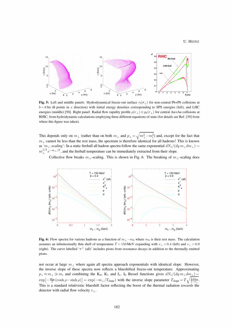
linearly with r⊥ [39, 47, 48]. As shown in the right panel of Fig. 5, it eventually reaches a maximum

value and drops again to zero since the dilute tail of the initial density distribution freezes out early

before radial flow develops. The left two panels of Fig. 5 show typical freeze-out surfaces τ f(r⊥) from

hydrodynamic calculations (see later) for SPS (left) and LHC energies (middle) [50]. One sees that

at SPS energies the freeze-out surface moves from the edge inward since the fireball matter cools and

freezes out faster than the developing radial flow can push it out. At LHC energies things begin similarly,

but then the much stronger radial flow generated by the much higher internal pressure makes the fireball

grow considerably before suddenly freezing out after about 13 fm/c. The freeze-out surface for RHIC

energies lies in between [51], with transverse flow almost exactly balancing freeze-out and leading to an

almost constant freeze-out radius (also seen in the right panel of Fig. 5) until after about 12 fm/c it rather

suddenly shrinks to zero, again indicating sudden bulk freeze-out.

So how does the radial flow affect the spectra? Looking at Eq. (26) we see that in the absence of

flow (ρ= 0) the second term vanishes (since I1(0)= 0) and the first term simply becomes (for constant

decoupling temperature)

dNi

dym⊥dm⊥∼ m⊥K1

(m⊥T

). (27)


181

0

4

8 02

46

8

0

5

10

15

y (fm)x (fm)

τ (fm

/c)

0

4

8 02

46

8

0

5

10

15

y (fm)x (fm)

τ (fm

/c)

Fig. 5: Left and middle panels: Hydrodynamical freeze-out surface τf(r⊥) for non-central Pb+Pb collisions at

b=8 fm (b points in x direction) with initial energy densities corresponding to SPS energies (left), and LHC

energies (middle) [50]. Right panel: Radial flow rapidity profile ρ(r⊥)≡ yT(r⊥) for central Au+Au collisions at

RHIC, from hydrodynamic calculations employing three different equations of state (for details see Ref. [39] from

where this figure was taken).

This depends only on m⊥ (rather than on both m⊥ and p⊥ =√m2

⊥−m2i ) and, except for the fact that

m⊥ cannot be less than the rest mass, the spectrum is therefore identical for all hadrons! This is known

as ‘m⊥-scaling’: In a static fireball all hadron spectra follow the same exponential dNi/(dy m⊥dm⊥) ∼m

1/2⊥ e−m⊥/T , and the fireball temperature can be immediately extracted from their slope.

Collective flow breaks m⊥-scaling. This is shown in Fig. 6. The breaking of m⊥-scaling does

0 0.5 1 1.5 2

10−4

10−3

10−2

10−1

100

π+ (all)

π+

K0s

pd

dN/(m

T dm

T) (ar

b. u

nits

)

mT − m0 (GeV)

T = 150 MeV β = 0.4

0 1 2 3 4

10−4

10−3

10−2

10−1

100

π+ (all)

π+

K0s

pd

dN/(m

T dm

T) (ar

b. u

nits

)

mT − m0 (GeV)

T = 150 MeV β = 0.9

Fig. 6: Flow spectra for various hadrons as a function of m⊥−m0 where m0 is their rest mass. The calculation

assumes an infinitesimally thin shell of temperature T =150 MeV expanding with v⊥ = 0.4 (left) and v⊥ =0.9

(right). The curve labelled ‘π+ (all)’ includes pions from resonance decays in addition to the thermally emitted

pions.

not occur at large m⊥ where again all spectra approach exponentials with identical slope. However,

the inverse slope of these spectra now reflects a blueshifted freeze-out temperature: Approximating

p⊥≈m⊥mi and combining the K0, K1 and I1, I0 Bessel functions gives dNi/(dy m⊥dm⊥)∼exp

[−m⊥

T (cosh ρ− sinh ρ)]= exp(−m⊥/Tslope) with the inverse slope parameter Tslope =T

√1+v⊥1−v⊥ .

This is a standard relativistic blueshift factor reflecting the boost of the thermal radiation towards the

detector with radial flow velocity v⊥.

U. HEINZ

182

Transverse flow breaks m⊥-scaling at small transverse momenta p⊥ . mi where momenta and

velocities can be added non-relativistically. The exact form of this breaking of m⊥ scaling depends on

the density and velocity profiles. It is most extreme for a thin shell expanding with fixed velocity (‘blast

wave’), shown in Fig. 6, in which case for sufficiently large hadron mass and flow velocity the spectrum

develops a ‘blast wave peak’ at non-zero transverse momentum [52]. More realistic calculations take

into account the integration over a velocity profile in which the hole at low p⊥ in the blast wave spectrum

is filled in by contributions with smaller radial boost velocities from the fireball interior [45]. For a

Gaussian density profile combined with a non-relativistic linear transverse velocity profile the integrated

spectrum can be calculated analytically [53], and one finds again an exponential m⊥-spectrum, but this

time with inverse slope Ti,slope =Tf + 12mi〈v⊥〉2. We summarize these two important limits:

• Non-relativistic, p⊥ mi : Ti,slope ≈ Tf +1

2mi〈v⊥〉2 . (28)

• Relativistic, p⊥ mi : Tslope ≈ Tf

√1+v⊥1−v⊥

(for all mi) . (29)

The slope systematics for hadrons with different masses in the low-p⊥ region thus allow us to separate

thermal from collective flow motion. Note that Eq. (28) can never be applied to pions since in the region

p⊥ mπ their slope is affected by Bose statistics and by the contamination from resonance decays (see

Fig. 6), neither of which is accounted for by Eq. (28).

4.1.8 Extracting the freeze-out temperature and flow from measured transverse momentum spectra

Equations (28) and (29) show that, as long as mi〈v⊥〉 & 2Tf, the spectra are steeper at high p⊥ and bend

over becoming flatter at low p⊥. It is therefore difficult to characterize them by a single slope, especially

when the detector measures different hadrons in different p⊥-windows, or when two different experi-

ments measure the same hadron in different p⊥-windows. To extract the flow velocity using Eq. (28)

requires measuring all hadrons in a common interval of nonrelativistic transverse kinetic energy satisfy-

ing m⊥−mi . mi. Since such a procedure throws away information outside the common window, it

is not very efficient. A much preferred method is to use the entire experimentally available information

on the spectra by performing a simultaneous fit to all hadrons over all m⊥ using Eq. (26). Assuming a

constant freeze-out temperature, a common shape for the density profiles ni(r⊥), and a specific shape

for τf(r⊥), we can rewrite Eq. (26) as an integral over flow rapidities [46],

dNi

dym⊥dm⊥= Ni

∫ ∞

0dρw(ρ)

[m⊥K1

(m⊥ cosh ρ

T

)I0

(p⊥ sinh ρ

T

)(30)

−p⊥∂τf

∂r⊥K0

(m⊥ cosh ρ

T

)I1

(p⊥ sinh ρ

T

)],

with the flow rapidity distribution

Ni w(ρ) =giπ2

r⊥(ρ)ni(r⊥(ρ))dr⊥dρ

(31)

where r⊥(ρ) is the inverse of the velocity profile ρ(r⊥). We see that for the shape of the spectrum the

density and velocity profiles ni(r⊥) and v⊥(r⊥) have no independent relevance — only the flow rapidity

distribution w(ρ) matters. If we fix a reasonable shape for w(ρ) (see [46]), leaving its mean 〈ρ〉 free,

we end up with a two-parameter fit in terms of the freeze-out temperature T =Tf and average transverse

flow velocity 〈v⊥〉 = tanh−1 〈ρ〉.Figure 7 shows such a fit to hadronic m⊥-spectra measured by the NA49 Collaboration [54] in

Pb+Pb collisions at the SPS at three different beam energies. Even disregarding the fitted lines, the flow-

typical hierarchy of slopes in the low-m⊥ region is obvious. The fit was done with a thin-shell model


183

0 0.5 1 1.5 210-5

10-3

10-1

10

103

-π

-K

0.1)×(p

0.01)× (Λ

φ

4 MeV±T=137 0.01±= 0.43 Tβ

/NDF=117/302χ

dy)

T d

mT

N/(

m2

d

10-5

10-3

10-1

10

103

-π+K

0.1)×p (

0.01)× (Λ

0.01)×d (

2 MeV±T=130

0.01±= 0.46 Tβ

/NDF=152/332χ

GeVA40

0 0.5 1 1.5 2

-π

-K

0.1)× (p

0.01)× (Λ

φ

1 MeV±T=120 0.01±= 0.47 Tβ

/NDF=106/382χ

-π+K

0.1)×p (

0.01)× (Λ

0.01)×d (

3 MeV±T=133

0.01±= 0.46 Tβ

/NDF= 43/372χ

GeVA80

(GeV)0-mTm0 0.5 1 1.5 2

-π

-K

0.1)× (p 0.01)× (Λ

φ

0.02)× (Ω

0.01)× (Ξ

2 MeV±T=114 0.01±= 0.50 Tβ

/NDF= 91/412χ

-π

+K 0.5)×p (

0.05)× (Λ

0.01)×d (

0.1)× (Ω

0.05)× (Ξ

1 MeV±T=127

0.01±= 0.48 Tβ

/NDF=120/432χ

GeVA158

Fig. 7: Positively and negatively charged hadron spectra from central Pb+Pb collisions at 40, 80 and 158AGeV

beam energy at the SPS, measured by the NA49 Collaboration [54]. Also shown are two-parameter fits with

Eq. (30), assuming a sharp transverse flow velocity βT [i.e., w(ρ)= δ(ρ− tanh−1 βT)] and constant τf. The result-

ing fit values for T and βT are given in the figures. Positive and negative hadrons were fitted independently; dashed

lines indicate hadrons which were not included in the fit. The dashed pion curve does not include resonance decay

contributions and Bose statistics.

with fixed radial flow velocity. As discussed above this tends to exaggerate the bending of the spectra at

low p⊥, especially for the heavier particles Ξ, Ω and the deuteron. This tendency can be seen in Fig. 7.

Otherwise the quality of the fit, its ability to describe all spectra simultaneously, and the consistency of

the fit parameters extracted from positively and negatively charged hadrons is impressive.

The flattening of the spectra at low transverse kinetic energy m⊥−m0 by transverse collective

flow is even more dramatic at RHIC. Figure 8 shows a direct comparison of the negative pion, kaon and

antiproton spectra in central Au+Au and minimum-bias proton–proton collisions, at the same centre of

mass energy. Clearly, in p+p collisions the kaon and antiproton spectra have the same slope, indicating

the absence of transverse collective flow. That the pion spectra are steeper than both kaons and antipro-

tons can be attributed to the contribution of resonance decay pions which accumulate at low transverse

momenta. However, the pion spectra are obviously flatter in Au+Au than in p+p, and this is even more

true for kaons and antiprotons, with a large difference in slope between these last two. Even without a

quantitative fit this is a clear manifestation of strong radial flow.

U. HEINZ

184

0 0.1 0.2 0.3 0.4 0.5 0.6 0.71

10

102

0 0.1 0.2 0.3 0.4 0.5 0.6 0.7

10-2

10-1

1

1/(

2π)

d2N

/ (

mT d

mT d

y)

[c

4/G

eV

2]

mT - m0 [GeV/c2] mT - m0 [GeV/c2]

1/(

2π)

d2N

/ (

mT d

mT d

y)

[c

4/G

eV

2]

STAR preliminary

Au+Au central

√sNN = 200 GeV

STAR preliminary

p+p min. bias

√sNN = 200 GeV

π-π-

K-

p

π-π-

K-

p

Fig. 8: Pion, kaon and

antiproton spectra from

200AGeV central Au+Au

(left) and minimum-bias p+p

(right) collisions, measured

by the STAR experiment [55].

Note the similar slopes for

kaons and antiprotons in p+p

collisions and their dramati-

cally different slopes at low

transverse kinetic energy in

central Au+Au collisions.

(M

eV

)fo

T

60

80

100

120

140

160

180

200PHENIX Preliminary

partN

0 50 100 150 200 250 300 350

Tβ

0.1

0.2

0.3

0.4

0.5

0.6

0.7

0.8

0.9

1

Fig. 9: Kinetic freeze-out temperature Tf

and transverse flow velocity βT at the fire-

ball edge, extracted from a simultaneous

fit of a flow spectrum parametrization to

π±, K±, p and p spectra from 200AGeV

Au+Au collisions over the entire range of

collision centralities [56]. More peripheral

collisions (small numbers Npart of partici-

pating nucleons) are seen to decouple ear-

lier, at higher freeze-out temperature and

with less transverse flow.

A two-parameter flow fit on RHIC data from 200A GeV Au+Au collisions was performed by

J. Burward-Hoy [56], see Fig. 9. Here a box-profile for the transverse density ni(r⊥) and a linear

transverse velocity profile were used, where the number βT given in Fig. 9 is the surface velocity (the

average transverse velocity is 〈v⊥〉 = 23βT). Again in the most central collisions freeze-out temperatures

of about 120 MeV and average radial flow velocities 〈v⊥〉' 0.45 are found. One should note, however,

that in this case the pions were included in the fit, without correction for resonance decay feed-down.

Resonance decay contributions steepen the pion spectrum, biasing the fit towards lower temperatures

and/or flow velocities. The bands in Fig. 9 attempt to provide an estimate of the systematic uncertainty

associated with details of the model assumptions on the density and velocity profile and of the p⊥ range

of the pion spectrum used in the fit [56].

An interesting aspect of Fig. 9 is the centrality dependence of the fit parameters: The fits were per-

formed over a very wide range of collision centralities, and one observes that more peripheral collisions


185

tend to develop less radial flow and freeze-out at a higher temperature. This is consistent with the expec-

tation that the collision fireballs in peripheral collisions do not live as long and have less time to build up

radial flow. However, even though their average flow is smaller, the flow gradients are bigger (because of

the smaller size), leading to decoupling at higher particle density and temperature. In pp collisions one

expects no or very little collectivity; Fig. 9 indicates that the transition to this limit in the most peripheral

Au+Au collisions is very steep, and that already a small number of nucleons participating in the collision

generates significant collectivity and sizeable radial flow.

Since the effects of the freeze-out temperature and flow on the spectral slope are strongly anti-

correlated [20], flow fits from single-particle spectra tend to produce narrow χ2 valleys in the T–〈v⊥〉plane, oriented from the upper left to the lower right. A direct comparison of the spectra from Pb+Pb

at the SPS and from Au+Au at RHIC shows that the RHIC spectra are flatter, especially for the heavier

hadrons [(anti)protons, (anti)Lambdas, etc. ] [46, 57]. So, when fitted with exactly the same procedure,

RHIC data give χ2 valleys which in the T–〈v⊥〉 plane lie to the upper right of those obtained from the

SPS data [46, 57]. At the same Tf they produce a somewhat larger flow, whereas with the same flow

RHIC data yield somewhat higher freeze-out temperatures [46]. In either case the effect is about 15%.

This flow analysis of the single-hadron spectra leads us to our first lesson: When the collision

is over and the hadron momentum spectra decouple, the fireball has a ‘thermal freeze-out temperature’

Tf ' 110− 130 MeV and is in a state of rapid transverse collective expansion with 〈v⊥〉 ' 0.45− 0.55 c(the ‘Little Bang’). These parameters have a systematic uncertainty ∼±10% and are strongly anticorre-

lated. In the T–〈v⊥〉 plane the χ2 valleys for the RHIC data are shifted systematically about 15% towards

the upper right compared with the SPS data.

4.1.9 Hydrodynamic calculation of radial flow

Of course, a flow fit to the spectra is just a fit, and there is no a priori guarantee that the extracted fit pa-

rameters make physical sense. In order to assess whether the extracted freeze-out temperatures and radial

flow velocities are physically meaningful we must check that they can be the result of reasonable models

for the dynamical evolution of the fireball. Is it possible to generate that much collective transverse flow

during the short lifetime of the collision zone before everything fizzles?

The natural language for studying flow phenomena is hydrodynamics. The hydrodynamic equa-

tions of motion are obtained from the local conservation laws for energy, momentum and baryon number,

∂µ Tµν(x) = 0 (ν = 0, . . . , 3) and ∂µj

µB(x) = 0 , (32)

by inserting the ideal fluid decompositions for the energy-momentum tensor and baryon number current:

T µν(x) =(e(x) + p(x)

)uµ(x)uν(x) − p(x) gµν , jµB(x) = nB(x)uµ(x) . (33)

These are 5 partial differential equations for 6 fields (p, e, nB and the 3 independent components of

uµ), and the system must be closed by providing an equation of state p(e, nB) for the fluid matter.

We use an equation of state which mimicks the lattice QCD results from Fig. 2 by matching a hadron

resonance gas below Tcr to an ideal gas of massless quarks and gluons above Tcr. For details I refer to

the literature [58, 59]. The numerical solution is considerably simplified by assuming Bjorken scaling

flow [41] along the beam direction [60] (see Section 4.1.4). The form of these simplified equations can

be found, e.g., in [58, 59]. They are solved for the transverse flow and hadron spectra near midrapidity

where, at sufficiently high collision energies, the assumption of longitudinal boost-invariance should

yield a good approximation. To obtain the entire rapidity distribution, on the other hand, requires a

solution of the full (3+1)-dimensional set of equations (see, e.g., Refs. [61, 62]) since boost-invariance

breaks down near the target and projectile rapidities.

As discussed in Section 3.4, the applicability of fluid dynamics requires mean free paths which are

short on any relevant macroscopic length scale. It can therefore not be used for the initial pre-equilibrium

U. HEINZ

186

stage of the collision just after nuclear impact nor for the very last stage when the matter becomes so

dilute that particles start to decouple. In addition to an equation of state (see Section 2.2), hydrodynamics

thus needs initial conditions for the time at which it starts to be a good approximation and for the energy

density, baryon number density and flow velocity profiles at that time, and a freeze-out algorithm which

tells us where to stop the hydrodynamic evolution and how to translate the hydrodynamic output (energy

and baryon densities and flow at freeze-out) into hadron spectra. For the freeze-out algorithm we use

the Cooper–Frye formula discussed in Section 4.1.5 with a constant freeze-out temperature. The initial

time, the initial entropy (or energy) and baryon density in the fireball, and the freeze-out temperature

(or equivalently the decoupling energy density) are treated as parameters to be adjusted to experimental

observables. The shape of the initial density profiles is calculated from the overlap geometry of the two

nuclei (for details see [63]). For the initial flow we assume a Bjorken scaling profile along the beam

direction (see Section 4.1.4) and zero initial transverse flow.

We thus need to fix four parameters, τeq, seq, nB,eq and edec. The ratio of the net baryon density

nB,eq to the entropy density seq is fixed by the measured proton/pion ratio. By entropy conservation, the

final total charged multiplicity dNch/dy fixes the initial product (s · τ)eq [41, 50, 60]. The value of τeq

controls how much transverse flow can be generated until freeze-out. It can thus be determined by trying

to fit simultaneously the final pion and proton spectra whose different slopes at low p⊥ are sensitive to

the radial flow at freeze-out. The associated freeze-out temperature, also implicit in these spectra, then

fixes the decoupling energy density edec.

0 1 2 3

10−2

100

102

pT (GeV)

1/ 2

π dN

/dyp

TdpT (G

eV−2

) π+ PHENIXp PHENIXp STARπ+ hydrop hydro

most central0 0.5 1 1.5 2 2.5

10−6

10−4

10−2

100

102

pT (GeV)

1/2π

dN

/dyp

TdpT (G

eV−2

) PHENIXSTARhydro

π−

0 − 5 %

5 − 15 %

15 − 30 %

30 − 60 %

60 − 92 %

centrality

0 1 2 3 410

−8

10−6

10−4

10−2

100 PHENIX

STARhydro

p

pT (GeV)

1/2π

dN

/dyp

TdpT (G

eV−2

)

0 − 5 %

5 − 15 %

15 − 30 %

30 − 60 %60 − 92 %

centrality

0 0.5 1 1.5 2

10−6

10−4

10−2

100

pT (GeV)

1/2π

dN

/dyp

TdpT (G

eV−2

)

PHENIXhydro

K+

0 − 5 %

5 − 15 %

15 − 30 %

30 − 60 %

60 − 92 %centrality

Fig. 10: Identified pion, antiproton and kaon spectra for√sNN = 130 GeV from the PHENIX [65, 69] and

STAR [66,67] collaborations in comparison with results from a hydrodynamic calculation [64]. The top left panel

shows pion and (anti-)proton spectra from central collisions. Shown in the other panels are spectra of five different

centralities: from most central (top) to the most peripheral (bottom). The spectra are successively scaled by a factor

of 0.1 for clarity.

The top left panel of Fig. 10 shows the hydrodynamic fit [64] to the transverse momentum spec-

tra of positive pions and antiprotons, as measured by the PHENIX and STAR collaborations in central


187

(b= 0) Au+Au collisions at√s= 130AGeV [65–67]. The fit yields an initial central entropy den-

sity seq =95 fm−3 at an equilibration time τeq = 0.6 fm. This corresponds to an initial temperature of

Teq = 340 MeV and an initial energy density e= 25 GeV/fm3 in the fireball centre. (Note that these pa-

rameters satisfy the ‘uncertainty relation’ τeq · Teq ≈ 1.) Freeze-out was implemented on a hypersurface

of constant energy density with edec =0.075 GeV/fm3. Table 1 summarizes the initial conditions applied

in hydrodynamic studies at SPS and RHIC energies (see the recent review [58] for references).

Table 1: Initial conditions for SPS and RHIC energies used to fit the particle spectra from central Pb+Pb or Au+Au

collisions. seq and Teq refer to the maximum values at τeq in the fireball centre.

SPS RHIC1 RHIC2√sNN (GeV) 17 130 200

seq (fm−3) 43 95 110

Teq (MeV) 257 340 360

τeq (fm/c) 0.8 0.6 0.6

The fit in the top left panel of Fig. 10 was performed with a chemical equilibrium equation of state.

Use of such an equation of state implicitly assumes that even below the hadronization temperature Tcr

chemical equilibrium among the different hadron species can be maintained all the way down to kinetic

freeze-out. With such an equation of state the decoupling energy edec = 0.075 GeV/fm3 translates into a

kinetic freeze-out temperature of Tdec ≈ 130 MeV. The data, on the other hand, show [68] that the hadron

abundances freeze out at Tchem ≈Tcr, i.e., even when hadrons first coalesce from the expanding quark–

gluon soup the inelastic processes which could transform different hadron species into each other are too

slow to keep up with the expansion. The measured p/π ratio thus does not agree with the one computed

from the chemical equilibrium equation of state at the kinetic freeze-out temperature Tdec = 130 MeV,

and the latter must be rescaled by hand if one wants to reproduce not only the shape, but also the correct

normalization of the measured spectra in Fig. 10.

A better procedure would be to use a chemical non-equilibrium equation of state for the hadronic

phase [70–72] in which for temperatures T below Tchem the chemical potentials for each hadronic species

are readjusted in such a way that their total abundances (after decay of unstable resonances) are kept

constant at the observed values. This approach has recently been applied [73] to newer RHIC data at√s=200AGeV.

Once the parameters have been fixed in central collisions, spectra at other centralities and for

different hadron species can be predicted without introducing additional parameters. The remaining

three panels of Fig. 10 show the transverse momentum spectra of pions, kaons and antiprotons in five

different centrality bins as observed by the PHENIX [65, 69] and STAR [66, 67] collaborations. For

all centrality classes, except the most peripheral one, the hydrodynamic predictions (solid lines) agree

pretty well with the data. The kaon spectra are reproduced almost perfectly, but for pions the model

consistently underpredicts the data at low p⊥. This has now been understood to be largely an artifact

of having employed in these calculations a chemical equilibrium equation of state all the way down to

kinetic freeze-out. More recent calculations [73] with a chemical non-equilibrium equation of state show

that, as the system cools below the chemical freeze-out point Tchem ≈Tcr, a significant positive pion

chemical potential builds up, emphasizing the concave curvature of the spectrum from Bose effects and

increasing the feed-down corrections from heavier resonances at low p⊥.

Significant discrepancies are also seen at large impact parameters and large transverse momenta

p⊥ & 2.5 GeV/c. This is not surprising since high-p⊥ particles require more rescatterings to thermalize

and escape from the fireball before doing so. This is in particular true in more peripheral collisions where

the reaction zone is smaller.

U. HEINZ

188

0 0.5 1 1.5 2 2.5

10−4

10−3

10−2

10−1

mT−m

0 (GeV)

1/(2

π) d

N/m

TdmTdy

(GeV

−2)

Ω − 200 AGeV

hydroα=0.02 fm−1

α=0.00

STAR prelim.

Fig. 11: Transverse mass spectrum of Ω hyperons from central 200AGeV Au+Au collisions at RHIC [74].

The curves are hydrodynamic calculations [73] with different initial and freeze-out conditions: Solid lines

correspond to the default of no initial transverse flow at τeq, dashed lines assume a small but non-zero ra-

dial flow, v⊥ = tanh(αr⊥) with α=0.02 fm−1, already at τeq. The lower (thin) set of curves assumes Ω-

decoupling at Tcr = 164 MeV, the upper (thick) set of curves decouples the Ω together with the pions and protons

at edec = 0.075 GeV/fm3. (In the chemical non-equilibrium hadronic equation of state employed here this value of

edec corresponds to a freeze-out temperature Tdec ≈ 100 MeV — see Ref. [73] for details.)

Figure 11 compares preliminary spectra of Ω hyperons [74] with hydrodynamic predictions [73,

75]. For this comparison the original calculations for 130AGeV Au+Au collisions [75] were repeated

with RHIC2 initial conditions and a chemical non-equilibrium equation of state in the hadronic phase

[73]. Following a suggestion that Ω hyperons, being heavy and not having any known strong coupling

resonances with pions, should not be able to participate in any increase of the radial flow during the

hadronic phase and thus decouple early [76], Fig. 11 shows two solid lines: The steeper one corresponds

to decoupling at edec = 0.45 GeV/fm3, i.e., directly after hadronization at Tcr, whereas the flatter one

assumes decoupling together with pions and other hadrons at edec = 0.075 GeV/fm3. The data clearly

favour the flatter curve, suggesting intense rescattering of the Ω’s in the hadronic phase. The microscopic

mechanism for this rescattering is still unclear. However, without hadronic rescattering the hydrodynamic

model, in spite of its perfect local thermalization during the early expansion stages, is unable to generate

enough transverse flow to flatten the Ω spectra as much as required by the data. Partonic hydrodynamic

flow alone can not explain the Ω spectrum. Similar comments apply to the Ω and Ω spectra from Pb+Pb

collisions at the SPS shown in Fig. 7.

We close this subsection by concluding that the freeze-out parameters extracted from flow fits to

the measured spectra are dynamically consistent, i.e., they can be reproduced in hydrodynamic calcula-

tions of the fireball evolution using realistic initial conditions. The successful hydrodynamic calculations

require fast thermalization at τeq . 1 fm/c and high initial energy density, eeq & 20 GeV/fm3. This con-

clusion will be solidified by the study of elliptic flow in the next subsection. The hydrodynamically

generated strong transverse flow naturally explains the much flatter proton than pion spectra at low p⊥(see Fig. 10). Together with the approximate baryon/antibaryon symmetry at RHIC (p/p≈ 0.7 in Au+Au

collisions), this provides a simple understanding for the initially puzzling observation that in Au+Au col-

lisions at RHIC for p⊥ & 2 GeV/c antiprotons are as abundant as negative pions (upper left panel in

Fig. 10). This is completely unexpected from standard string and jet fragmentation phenomenology in

pp and e+e− collisions where the p/π− ratio never exceeds 10–15%, but is a simple (albeit dramatic)

consequence of the collective transverse flow in heavy-ion collisions.


189

4.2 Elliptic flow

4.2.1 Anisotropic flow in non-central collisions

For central collisions (b= 0) between equal spherical nuclei, radial flow (left panel of Fig. 12) is the

only possible type of transverse flow allowed by symmetry. In non-central (b 6= 0) collisions between

b−10 −5 0 5 10

−10

−5

0

5

10

x (fm)

y (fm

)

Fig. 12: Left and centre panels: Schematic picture of radial and elliptic flow. Right panel: Initial energy density

contours in the transverse plane for a Au+Au collision at impact parameter b=7 fm. The dashed circles indicate

transverse projections of the colliding nuclei.

spherical nuclei (right panels of Fig. 12), or in b= 0 collisions between suitably aligned deformed nuclei

(such as 238U), this azimuthal symmetry is broken and anisotropic transverse flow patterns can develop.

The overlap region of the two colliding nuclei is then spatially deformed in the transverse plane, i.e., the

spatial eccentricity of the reaction zone

εx(b) =

⟨y2 − x2

⟩

〈y2 + x2〉 (34)

(where the average is taken with the energy density distribution) is initially non-zero and positive. Rescat-

tering processes among the produced particles transfer this spatial deformation onto momentum space,

i.e. the initially locally isotropic transverse momentum distribution of the produced matter begins to

become anisotropic. The driving force for this momentum anisotropy is the spatial eccentricity; the

momentum anisotropy can only grow as long as εx> 0. As a function of time εx decreases, either spon-

taneously due to free-streaming radial expansion (if no rescattering happens) or somewhat more quickly

due to the development of elliptic flow (if rescattering occurs) which makes the system expand faster into

the reaction plane than perpendicular to it (see middle panel in Fig. 12). Once the spatial eccentricity has

disappeared, the momentum anisotropy saturates [77]. Since this happens quite early in the collision (as

we will see shortly), the finally observed momentum anisotropy opens a window onto the early stage of

the fireball expansion.

The mechanism for the creation of elliptic flow is most easily understood in the hydrodynamic

limit: After thermalization there is high pressure in the interior of the reaction zone which falls off to

zero outside. Obviously the pressure gradient is steeper in the short direction, leading to stronger hy-

drodynamic acceleration into the reaction plane. This is seen in Fig. 13 where I show hydrodynamically

computed energy density contours and flow vector fields for non-central Pb+Pb collisions for 4 different

times after the onset of hydrodynamic expansion. One sees that the reaction zone expands faster into the

reaction plane and that the spatial eccentricity is almost gone after about 8 fm/c.

U. HEINZ

190

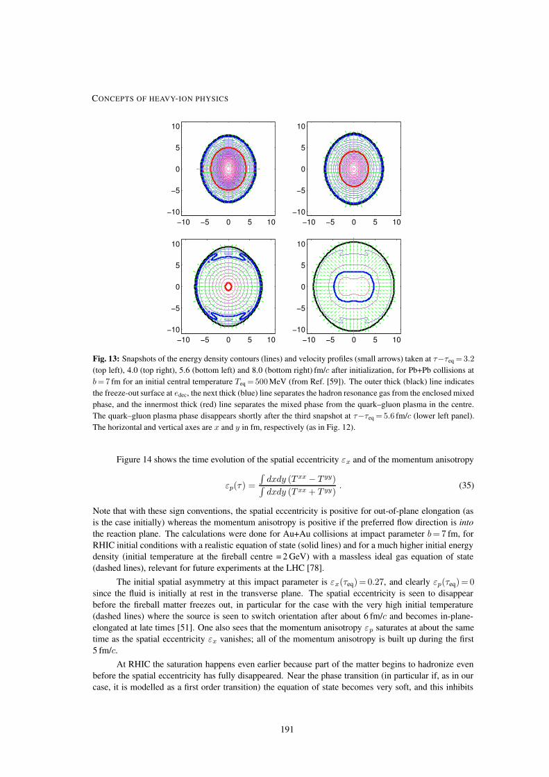
−10 −5 0 5 10−10

−5

0

5

10

−10 −5 0 5 10−10

−5

0

5

10

−10 −5 0 5 10−10

−5

0

5

10

−10 −5 0 5 10−10

−5

0

5

10

Fig. 13: Snapshots of the energy density contours (lines) and velocity profiles (small arrows) taken at τ−τeq =3.2

(top left), 4.0 (top right), 5.6 (bottom left) and 8.0 (bottom right) fm/c after initialization, for Pb+Pb collisions at

b=7 fm for an initial central temperature Teq =500 MeV (from Ref. [59]). The outer thick (black) line indicates

the freeze-out surface at edec, the next thick (blue) line separates the hadron resonance gas from the enclosed mixed

phase, and the innermost thick (red) line separates the mixed phase from the quark–gluon plasma in the centre.

The quark–gluon plasma phase disappears shortly after the third snapshot at τ−τeq = 5.6 fm/c (lower left panel).

The horizontal and vertical axes are x and y in fm, respectively (as in Fig. 12).

Figure 14 shows the time evolution of the spatial eccentricity εx and of the momentum anisotropy

εp(τ) =

∫dxdy (T xx − T yy)∫dxdy (T xx + T yy)

. (35)

Note that with these sign conventions, the spatial eccentricity is positive for out-of-plane elongation (as

is the case initially) whereas the momentum anisotropy is positive if the preferred flow direction is into

the reaction plane. The calculations were done for Au+Au collisions at impact parameter b= 7 fm, for

RHIC initial conditions with a realistic equation of state (solid lines) and for a much higher initial energy

density (initial temperature at the fireball centre = 2 GeV) with a massless ideal gas equation of state

(dashed lines), relevant for future experiments at the LHC [78].

The initial spatial asymmetry at this impact parameter is εx(τeq)= 0.27, and clearly εp(τeq)= 0since the fluid is initially at rest in the transverse plane. The spatial eccentricity is seen to disappear

before the fireball matter freezes out, in particular for the case with the very high initial temperature

(dashed lines) where the source is seen to switch orientation after about 6 fm/c and becomes in-plane-

elongated at late times [51]. One also sees that the momentum anisotropy εp saturates at about the same

time as the spatial eccentricity εx vanishes; all of the momentum anisotropy is built up during the first

5 fm/c.

At RHIC the saturation happens even earlier because part of the matter begins to hadronize even

before the spatial eccentricity has fully disappeared. Near the phase transition (in particular if, as in our

case, it is modelled as a first order transition) the equation of state becomes very soft, and this inhibits


191

Fig. 14: Time evolution of the spa-

tial eccentricity εx and the momentum

anisotropy εp for Au+Au collisions with

b=7 fm at RHIC and at much higher col-

lision energies (from Ref. [78]).

the generation of transverse flow. This also affects the generation of transverse flow anisotropies, as seen

from the solid curves in Fig. 14: The rapid initial rise of εp suddenly stops as a significant fraction of the

fireball matter enters the mixed phase. It then even decreases somewhat as the system expands radially

without further acceleration, thereby becoming more isotropic in both coordinate and momentum space.

Only after the phase transition is complete and pressure gradients reappear, does the system react to the

remaining spatial eccentricity by a slight further increase of the momentum anisotropy. The softness of

the equation of state near the phase transition thus focuses the generation of anisotropic flow to even

earlier times, when the system is still entirely partonic and has not even begun to hadronize. At RHIC

energies this means that almost all of the finally observed elliptic flow is created during the first 3–

4 fm/c of the collision and reflects the hard QGP equation of state of an ideal gas of massless particles

(c2s = 13 ) [59]. Microscopic kinetic studies of the evolution of elliptic flow lead to similar estimates for

this time scale [77, 79–81].

4.2.2 The elliptic flow coefficient v2

The momentum anisotropy εp manifests itself as an azimuthal anisotropy of the measured hadron spectra.

One quantifies this anisotropy in terms of the azimuthal Fourier coefficients of the transverse momentum

spectrum:dNi

dy p⊥dp⊥ dϕp(b) =

1

2π

dNi

dy p⊥dp⊥(b)

(1 + 2 vi2(p⊥, b) cos(2ϕp) + . . .

). (36)

These coefficients depend on the impact parameter b, the transverse momentum p⊥ and the particle

species i (through their rest mass mi). We have suppressed the dependence on rapidity y since the cal-

culation assumes longitudinal boost-invariance and thus makes meaningful statements only near y= 0.

At midrapidity v2 is (for collisions between equal nuclei) the lowest nonvanishing Fourier coefficient.

Reflection symmetry with respect to the reaction plane forbids the appearance of sine terms in the ex-

pansion. Equation (36) implies that the elliptic flow coefficient can be calculated as

vi2(p⊥, b) = 〈cos(2ϕp)〉ip⊥,b (37)

where the average is performed with the transverse momentum spectrum of particle species i at fixed

impact parameter and p⊥. If the average is performed with the p⊥-integrated spectrum one obtains the

‘p⊥-integrated elliptic flow’ vi2(b).

Figure 15 shows a comparison of elliptic flow data for charged hadrons from Au+Au collisions

at RHIC with hydrodynamic calculations. The hydrodynamic results are genuine predictions since all

model parameters have been fixed in central (b= 0) collisions where v2 vanishes. The impact param-

eter dependence of v2(p⊥) then follows from the overlap geometry and its implications for the initial

transverse density profile and its spatial eccentricity [63], without additional parameters. The data follow

U. HEINZ

192

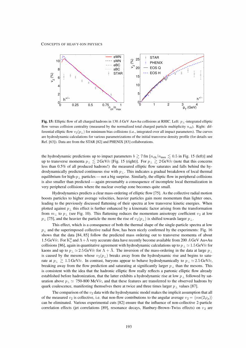
0 0.25 0.5 0.75 10

2

4

6

8

10

nch

/nmax

v 2 (%)

eWNsWNeBCsBCSTAR

h+/−

0 1 2 3 40

5

10

15

20

25

pT (GeV)

v 2 (%) STAR

PHENIXEOS QEOS H

h+/−

Fig. 15: Elliptic flow of all charged hadrons in 130AGeV Au+Au collisions at RHIC. Left: p⊥-integrated elliptic

flow versus collision centrality (measured by the normalized total charged particle multiplicity nch). Right: dif-

ferential elliptic flow v2(p⊥) for minimum bias collisions (i.e., integrated over all impact parameters). The curves

are hydrodynamic calculations for various parametrizations of the initial transverse density profile (for details see

Ref. [63]). Data are from the STAR [82] and PHENIX [83] collaborations.

the hydrodynamic predictions up to impact parameters b & 7 fm [nch/nmax . 0.5 in Fig. 15 (left)] and

up to transverse momenta p⊥ . 2 GeV/c [Fig. 15 (right)]. For p⊥ & 2 GeV/c (note that this concerns

less than 0.5% of all produced hadrons!) the measured elliptic flow saturates and falls behind the hy-

drodynamically predicted continuous rise with p⊥. This indicates a gradual breakdown of local thermal

equilibrium for high-p⊥ particles — not a big surprise. Similarly, the elliptic flow in peripheral collisions

is also smaller than predicted — again presumably a consequence of incomplete local thermalization in

very peripheral collisions where the nuclear overlap zone becomes quite small.

Hydrodynamics predicts a clear mass-ordering of elliptic flow [75]. As the collective radial motion

boosts particles to higher average velocities, heavier particles gain more momentum than lighter ones,

leading to the previously discussed flattening of their spectra at low transverse kinetic energies. When

plotted against p⊥ this effect is further enhanced by a kinematic factor arising from the transformation

from m⊥ to p⊥ (see Fig. 10). This flattening reduces the momentum anisotropy coefficient v2 at low

p⊥ [75], and the heavier the particle the more the rise of v2(p⊥) is shifted towards larger p⊥.

This effect, which is a consequence of both the thermal shape of the single-particle spectra at low

p⊥ and the superimposed collective radial flow, has been nicely confirmed by the experiments: Fig. 16

shows that the data [84, 85] follow the predicted mass ordering out to transverse momenta of about

1.5 GeV/c. For K0s and Λ+Λ very accurate data have recently become available from 200AGeV Au+Au

collisions [86], again in quantitative agreement with hydrodynamic calculations up to p⊥' 1.5 GeV/c for

kaons and up to p⊥' 2.5 GeV/c for Λ + Λ. The inversion of the mass-ordering in the data at large p⊥is caused by the mesons whose v2(p⊥) breaks away from the hydrodynamic rise and begins to satu-

rate at p⊥ & 1.5 GeV/c. In contrast, baryons appear to behave hydrodynamically to p⊥' 2.5 GeV/c,breaking away from the flow prediction and saturating at significantly larger p⊥ than the mesons. This

is consistent with the idea that the hadronic elliptic flow really reflects a partonic elliptic flow already

established before hadronization, that the latter exhibits a hydrodynamic rise at low p⊥ followed by sat-

uration above p⊥' 750-800 MeV/c, and that these features are transferred to the observed hadrons by

quark coalescence, manifesting themselves there at twice and three times larger p⊥ values [87].

The comparison of the v2 data with the hydrodynamic model makes the implicit assumption that all

of the measured v2 is collective, i.e. that non-flow contributions to the angular average v2 = 〈cos(2ϕp)〉can be eliminated. Various experimental cuts [82] ensure that the influence of non-collective 2-particle

correlation effects (jet correlations [89], resonance decays, Hanbury-Brown–Twiss effects) on v2 are


193

0 0.25 0.5 0.75 10

5

10

pT (GeV)

v 2 (%)

π+ + π−

p + p

STARhydro EOS Qhydro EOS H

0 0.5 1 1.5 2 2.5 3 3.5 4

-0.05

0

0.05

0.1

0.15

0.2

0.25

0.3

0 0.5 1 1.5 2 2.5 3 3.5 4

-0.05

0

0.05

0.1

0.15

0.2

0.25

0.3

pT (GeV/c)pT (GeV/c)

V2 V2

identified hadrons (-) v2

( |η| < 0.35, min. bias, R.P. |η| = 3~4 )PHENIX Preliminary

identified hadrons (+) v2

( |η| < 0.35, min. bias, R.P. |η| = 3~4 )PHENIX Preliminary

π-K-pbar

π+K+phydro calc.hydro calc.

Fig. 16: Differential elliptic flow for identified pions, kaons and (anti)protons from Au+Au collisions at√sNN =130 GeV [84] (left) and at

√sNN = 130 GeV [85] (right), together with hydrodynamic calculations [64].

minimized. An alternative method to extract v2 from higher-order cumulants of the azimuthal particle

distribution [90,91] has recently shown [92] that, in the interesting range p⊥ . 2 GeV/c where the emit-

ted hadrons behave hydrodynamically, non-flow corrections do not exceed 15% of the value extracted

from the prescription v2 = 〈cos(2ϕp)〉. (This may be different at much higher p⊥ where v2 from 2-

particle angular correlations seems to approach a p⊥-independent constant value [93], but statistics are

not good enough for a 4-particle cumulant analysis which could exclude that at high p⊥ an increasing

fraction of this v2 stems from angular 2-particle jet correlations.) Further support for the collective na-

ture of the measured v2 comes from the observation that the event plane angles reconstructed from v2 at

forward and backward rapidities are, within the statistical error, perfectly correlated. We can therefore

assume that at least 85% of the measured v2 values shown in Figs. 15–17 are due to collective flow.

4.2.3 Rapid thermalization and early pressure — the creation of the QGP

I already mentioned that momentum anisotropies, in particular elliptic flow, can only build as long as the

source is spatially deformed. Even if the created particles do not rescatter but simply fly off ballistically

with their isotropically distributed initial momenta, the spatial eccentricity decreases as a function of

time as [59]

εx(τ0+∆τ)

εx(τ0)=

[1 +

(c∆τ)2

〈r2〉τ0

]−1

, (38)

where τ0 is the time when the particles were created and⟨r2

⟩τ0

is the azimuthally averaged initial

transverse radius squared of the reaction zone. So if thermalization is delayed by a time ∆τ , any elliptic

flow would have to build on a reduced spatial deformation and would come out smaller.

It is also known from microscopic kinetic studies [80, 81] that for a given collision geometry, i.e.,

a given initial spatial eccentricity εx, the magnitude of the generated elliptic flow is a monotonic function

of the mean free path (or the product of density and scattering cross-section) in the fireball. This is shown

in Fig. 17. Without reinteractions (i.e., for infinite mean free path) no momentum anisotropies develop

at all [80]; the maximal value for v2 is reached in the hydrodynamic limit of zero mean free path [88].

This hydrodynamic upper limit for the charged particle elliptic flow was shown to be insensitive to

shape details of the initial transverse density distribution [63] and, as long as the shape and normalization

of the single particle spectra from central collisions were held fixed by proper retuning of the initial

conditions, any sensitivity to details of the QGP equation of state remained below 25% [75]. (Note that

this statement refers to the v2 of all charged particles which are strongly dominated by pions and kaons;

U. HEINZ

194

Fig. 17: Impact parameter averaged ellip-

tic flow as a function of transverse momen-

tum. The experimental data points from

STAR [82] are compared with parton cas-

cade calculations [81] with varying trans-

port opacities ξ (from [81]).

Fig. 16 (left) shows that the elliptic flow of heavier particles such as protons, which are more sensitive to

radial flow, shows indeed significant dependence on the equation of state, and that the data disfavour, for

example, a pure hadron resonance gas over an equation of state with a deconfining phase transition and

a hard QGP equation of state above Tcr.)

The observation that for b . 8 fm and p⊥ . 1.5–2 GeV/c the measured v2 exhausts at least 85%

of the hydrodynamically predicted value thus puts severe constraints on the dynamical evolution and on

our global picture of the collision event. It requires early thermalization (such that the spatial eccentricity

does not decay before elliptic flow starts to build) and almost complete local equilibrium throughout the

crucial first 5 fm/c of the expansion when the momentum anisotropies are generated. The hydrodynamic

model calculations for RHIC were done with a thermalization time τeq = 0.6 fm/c; increasing τeq beyond

1 fm/c not only begins to seriously degrade the description of the angle-averaged single-particle spectra,

but also cuts down v2 below the experimentally measured level. To obtain the full measured amount of

elliptic flow requires almost complete thermalization in less than 1 fm/c.

The sensitivity of v2 to any kind of deviation from local thermal equilibrium seems to be particu-

larly strong [94, 95]. (Of course, we are talking here about the momentum distribution for particles with

average momenta p⊥∼ 3T ; no claim for thermalization can be made for particles with much larger than

average p⊥ because they are too rare to affect bulk properties such as the pressure and the hydrodynamic

expansion.) Turning this observation around and remembering that most of the momentum anisotropy

is generated at energy densities well above the critical value for hadronization, the good agreement of

the data with ideal fluid dynamics points to a very small viscosity of the QGP. (Note my use of the word

QGP for the matter in the early expansion stage! What other name could I use for a thermalized sys-

tem of strongly interacting matter at energy densities > 10 ecr?) The QGP does not behave as a weakly

interacting quark–gluon gas, as suggested by naive perturbation theory, nor does it behave like viscous

honey, as suggested by the value of the shear viscosity extracted from state-of-the-art resummed thermal

field theory at leading order in the strong coupling constant [36]. The fact that the QGP behaves like an

ideal fluid implies strong non-perturbative interactions in the QGP phase.

So here is our second lesson: The strong measured elliptic flow at RHIC requires rapid thermaliza-

tion at τeq . 1 fm/c. At this time the average energy density in the thermalized fireball is e & 10−15ecr ,

so thermalization leads into a QGP state. In Au+Au collisions at RHIC this QGP lives for about 5–7 fm/cbefore hadronizing.


195

So what about the SPS? Have we made QGP there, too [10]? The energy densities were sufficient

(e & 3.5 GeV/fm3) and, at the 30% accuracy level, hydrodynamics did a good job for the angle-averaged

single-particle spectra from S+S and Pb+Pb collisions at the SPS, too [20,96]. However, the measured el-

liptic flow at the SPS is only about 50% of the value measured at RHIC [97,98], whereas hydrodynamics

predicts it to be in fact slightly larger than at RHIC [59]1. So thermalization seems to be less efficient at

the SPS than at RHIC. This may not be unreasonable, given the significantly lower (by about a factor of

3 [59]) initial density and the rapid conversion of the matter to a less strongly coupled hadron resonance

gas before the momentum anisotropy has been able to reach saturation. It would be good to test this with

central U+U collisions at the lower end of the collision energy range of RHIC [59]. Such collisions pro-

vide similar spatial eccentricities εx as semiperipheral Au+Au collisions, but for a fireball which covers

a much larger transverse area. This should improve thermalization at lower energies too, making hydro-

dynamics a better approximation, and help to test our understanding of the dynamical origin of elliptic

flow. I should also mention that at RHIC hydrodynamics fails to reproduce the rapidity dependence of

elliptic flow, predicting a wide rapidity plateau for v2 [72] whereas the measured elliptic flow rapidly

decreases as one moves away from midrapidity [99]. The origin of this discrepancy is not yet clear, but I

suspect that it again indicates a breakdown of local equilibrium away from midrapidity [100], for reasons

which are related to the analogous breakdown at midrapidity at lower collision energies [101].

5 Two-particle Bose–Einstein correlations and HBT interferometry

Single-particle momentum spectra, including their anisotropies, provide no direct information on the

space-time structure of the source. It is therefore in principle possible to describe these spectra with

models that have the same momentum structure but completely different freeze-out distributions in space

and time. Two-particle correlations, on the other hand, depend on the average separation of the particles

at decoupling and therefore provide valuable spatial and temporal information. This is most easily seen

for correlations generated by final state Coulomb interactions between charged hadrons which influence

their distribution of relative momenta depending on how close they were at time of emission. The

measured relative momentum distribution of particle pairs thus allows us to constrain their average space-

time distance at decoupling. Conceptually more involved, but theoretically easier to analyse, are two-

particle momentum correlations between pairs of identical particles (‘Bose–Einstein correlations’ in the

case of identical bosons) caused by quantum statistical (wave function symmetrization) effects. Again,

these affect the relative momentum distribution at low relative momenta, and the relative momentum

range of these quantum statistical correlations yields information about the average space-time separation

of the emission points of the two particles, and thereby also about the overall size and emission duration

of the source. There exist a number recent reviews of these methods to which I refer the reader for more

details [102–105].

For pairs of identical bosons (e.g., pions), this technique is known as Hanbury-Brown–Twiss

(HBT) interferometry [106]. The basic principle, as applied in particle and nuclear physics, is illus-

trated in Fig. 18. I will now shortly outline its theoretical treatment, referring to the literature [102–105]

for more details.

5.1 Single-particle spectra and two-particle correlations

The covariant single- and two-particle distributions are defined by

P1(p) = EdN

d3p= E 〈a+

p ap〉 , (39)

P2(p1,p2) = E1E2dN

d3p1d3p2= E1E2 〈a+

p1a+

p2ap2

ap1〉 , (40)

1At the SPS most of the elliptic flow is generated in the hadronic phase, and the softening effects of the phase transition on

the development of flow are not as important as at RHIC [59].

U. HEINZ

196

aa

ab

bb

11

12

22

pa1→ pb1

→ p1→

R→

R→ L→

d

θ

→

d→

~~~~

pb1→ pb2

→ pb→

~~ ~~

pa2→

pb2→

p2→ ~~~~

~

pa1

→ pa2

→ pa→

~~~

(c)

(b)

(a)

Fig. 18: The principle of two-particle interferometry: a pair of indistinguishable particles is emitted from points a

and b and detected by detectors 1 and 2 which measure their momenta p1 and p2. The total pair yield is obtained

by integrating over all possible positions (a, b) in the source. The measurement is performed as a function of the

average momentum K = (p1 + p2)/2 of the pair and its relative momentum q = p1 − p2. The q-dependence

yields information about the average separation 〈R2〉1/2 of the emitters a and b which contribute pairs of given

pair momentum K .

where a+p and ap create and destroy a particle with momentum p, respectively. The angular brackets

denote an ensemble average 〈O〉 = tr (ρO) where ρ is the density operator associated with the ensemble.

(When talking about an ensemble we may think of either a single large, thermalized source, or a large

number of similar, but not necessarily thermalized collision events.) The single-particle spectrum is

normalized to the average number of particles, 〈N〉, per collision,∫d3p

EP1(p) = 〈N〉 , (41)

whereas the two-particle distribution is normalized to the number of particles in pairs, 〈N(N − 1)〉, per

event: ∫d3p1

E1

d3p2

E2P2(p1,p2) = 〈N(N − 1)〉 . (42)

The two-particle correlation function is defined as

C(p1,p2) =P2(p1,p2)

P1(p1)P1(p2). (43)

If the two particles are emitted independently and final state interactions are neglected one can prove a

generalized Wick theorem [107, 108],

C(p1,p2) = 1 ±|〈a+

p1ap2

〉|2

〈a+p1 ap1

〉〈a+p2 ap2

〉. (44)

This assumption is often called ‘chaoticity assumption’, having in mind a completely chaotic (uncor-

related) emitter, in contrast to processes where the phases of the wave functions of the two emitted

particles are to some extent correlated with each other. The degree of ‘chaoticity’ or ‘phase correlation’

in the source can be studied by comparing three-particle correlations with two-particle ones [109]. This

was recently done by the STAR collaboration [110] who established that in central Au+Au collisions at√sNN =130 GeV the pion-emitting source is indeed completely chaotic.

From now on I will assume that the emitted particles are bosons, e.g., pions, and use the + sign in

Eq. (44). We next discuss the numerator of the Bose–Einstein correlation term, |〈a+p1ap2

〉|2.


197

5.2 Source Wigner function and spectra

As reviewed in Refs. [103, 107, 108], the pion-emitting source can be described in terms of classical

currents J(x) which act as classical sources of freely propagating pions. These currents represent a

parametrization of the last collision from which the free outgoing pion emerges. Using this language in

one form or another [103, 107, 108], one can express the ‘exchange amplitude’ 〈a+p1ap2

〉 as the Fourier

transform of the single-particle Wigner density S(x,K) which is the quantum mechanical analogue of

the classical phase-space density at pion freeze-out, describing the probability of emitting a pion with

momentum K from space-time point x:

〈a+p1ap2

〉 =

∫d4xS(x,K) eiq·x , (45)

S(x,K) is also called ‘emission function’. K = 12(E1+E2,p1+p2) is the average momentum of the

pair and q = (E1−E2,p1−p2) is the relative momentum between the two pions. Since the pion momenta

p1,p2 are on-shell, p0i = Ei = (m2 + p2

i )1/2, the four-momenta q and K are in general off-shell. They

satisfy the orthogonality relation (‘on-shell constraint’)

q ·K = 0 =⇒ q0 = β · q with β =K

K0≈ K

EK. (46)

β is the velocity of the pair; the last, so-called ‘on-shell’ approximation holds for small relative momenta

q, which is where the correlation term is non-zero:

K0 = EK

(1 +

q2

8E2K

+ O(

q4

E4K

))≈ EK . (47)

Since the relevant range of q is given by the inverse size of the source (more properly: the inverse size

of the regions of homogeneity in the source, see below), the validity of this approximation is ensured in

practice as long as the Compton wavelength of the particles is small compared to this ‘source size”. For

the case of pion, kaon, or proton interferometry for heavy-ion collisions this is true automatically owing

to the rest mass of the particles: even for pions at rest, the Compton wavelength of 1.4 fm is comfort-

ably smaller than any typical nuclear source size. This is of enormous practical importance because it

allows you essentially to replace the source Wigner density by a classical phase-space distribution func-

tion for on-shell particles. This provides a necessary theoretical foundation for the calculation of HBT

correlations from classical hydrodynamic or kinetic (e.g., cascade) simulations of the collision.

With the definition (45) we can express the single-particle spectra (39) and correlation function

(44) through the emission function S(x,K):

EpdN

d3p=

∫d4xS(x, p) , (48)

C(q,K) = 1 +(P1(K))2

P1(K+ 12q)P1(K− 1

2q)

∣∣∣∣∫d4x eiq·x S(x,K)∫d4xS(x,K)

∣∣∣∣2

≈ 1 +

∣∣∣∣∫d4x eiq·x S(x,K)∫d4xS(x,K)

∣∣∣∣2

≡ 1 +∣∣〈eiq·x〉

∣∣2 . (49)

The last line uses the ‘smoothness approximation’ P1(K+ 12q)P1(K− 1

2q) ≈ |P1(K)|2 which can be

justified for sufficiently large sources. It is not really necessary because the single-particle spectra are

measured and the ratio |P1(K)|2/P1(K+ 12q)P1(K−1

2q) can thus be divided out from the correlator

C(q,K) − 1 before analysing it theoretically, but we use it here for simplicity.

The last equality in Eq. (49) introduces the notation 〈f(x)〉 for the average of a space–time observ-

able f(x) with the emission function S(x,K). Note that, owing to the K-dependence of the emission

function, this average depends on the pair momentum K.

U. HEINZ

198

The fundamental relations (48) and (49) show that both the single-particle spectrum and the two-

particle correlation function can be expressed as simple integrals over the emission function. Whereas

the single-particle momentum spectrum (48) integrates over the spatial structure of the emission function

and thus provides no spatial information about the source, Eq. (49) shows that the q-dependence of the

correlation function C(q,K) provides access to the space-time structure of the source. However, it de-

pends only on the modulus square of the spatial Fourier transform of the source, so the phase information

is missing, and furthermore, owing to the ‘on-shell constraint’ (46), not all four components of q can be

varied independently. The Fourier transform in Eq. (49) thus mixes space and time in a particular way,

and the emission function S(x,K) cannot be fully reconstructed from the measured correlation func-

tion C(q,K) without taking recourse to model assumptions about the source. Still, as I will now show,

the correlator C(q,K) provides very important constraints for any dynamical model for the heavy-ion

collision.

5.3 HBT radii and source sizes

The most interesting feature of the two-particle correlation function is its half-width as a function of q.

Actually, since the relative momentum q = p1−p2 has three Cartesian components, the fall-off of the

correlator for increasing q is not described by a single half-width, but rather by a (symmetric) 3×3 tensor.

Through the Fourier transform in Eq. (49), these half-widths of the correlator (at a given pair momentum

K) can be related to the widths of the emission function S(x,K) in space and time (at the same K).

This relation becomes exact if particle emission is not complicated by processes involving multiple time

scales. Multiple time scales, with corresponding dynamically induced multiple length scales, are an

issue in pion emission from heavy-ion collisions: A large fraction of the observed pions is not emitted

from the source directly, but appears later from the decay of unstable resonances which were originally

emitted directly from the source but then travelled a certain distance without interactions before decaying.

Resonance decay effects on the HBT correlation function have been extensively discussed in the literature

(see, for example, Refs. [111, 112]). The results can be briefly summarized: Most resonances are so

short-lived that they do not travel far before decaying, leading to a pion emission function of almost the

same size and shape as for directly emitted pions. Some resonances are very long-lived and decay far

outside the original source; the corresponding temporal and spatial tails in the emission function affect

the correlator at such small values of q that they can not be experimentally resolved. They effectively

reduce the visible Bose–Einstein correlation strength and can be absorbed by reducing the second term

in Eq. (49) by a K-dependent ‘intercept parameter’ λ(K): C(q,K) = 1+λ(K)|〈eiq·x〉dir|2(K) where

〈. . . 〉dir denotes the average with the emission function for (almost) directly emitted pions. The only

resonance that can neither be classified as short-lived nor as long-lived in this sense is the ω meson with

its lifetime of about 20 fm/c. I will assume here that its abundance is small enough to be negligible

(this depends on the freeze-out temperature), but this is mostly for didactical purposes and needs to be

reassessed in the actual comparison between theory and data.

With these assumptions the ‘direct’ emission function can be fully characterized by its ‘widths’,

which depend on K:

Sµν(K) = [〈xµxν〉dir − 〈xµ〉dir〈xν〉dir〉] (K) ≡ 〈xµxν〉dir , (50)

which describe the widths of the effective emission region inside the source (‘homogeneity region’) that

effectively contributes to the emission of particles with momentum K. Note that for an expanding source

these effective emission regions do not coincide with the entire source: As illustrated in Fig. 19, pions

whose momentum K is large and points in the positive x direction will predominantly originate from

the elliptic region near the right edge of the figure, since this region anyway moves collectively in the

+x direction. On the other hand, the elliptic region near the top of the figure moves in the +y direction

and thus mostly contributes pions with (large) positive y-momentum Ky. Equation (49) shows that

the correlation function C(q,K) of pairs with pair momentum K probes only these effective emission


199

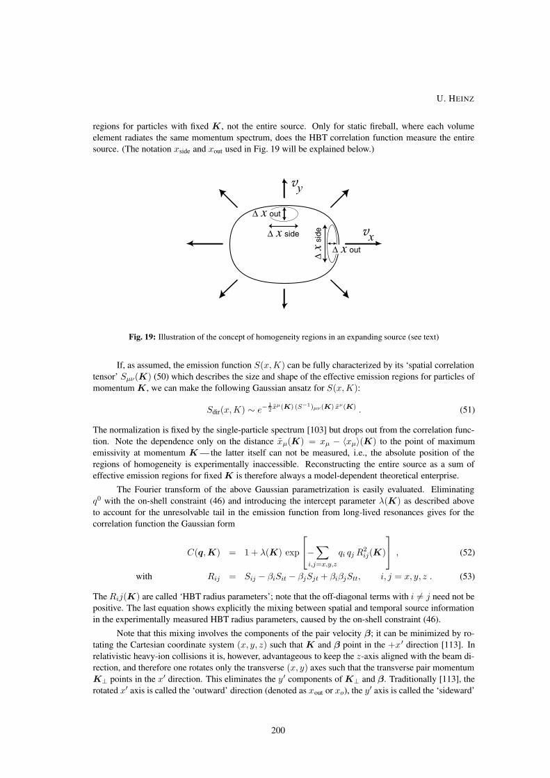
regions for particles with fixed K, not the entire source. Only for static fireball, where each volume

element radiates the same momentum spectrum, does the HBT correlation function measure the entire

source. (The notation xside and xout used in Fig. 19 will be explained below.)

Fig. 19: Illustration of the concept of homogeneity regions in an expanding source (see text)

If, as assumed, the emission function S(x,K) can be fully characterized by its ‘spatial correlation

tensor’ Sµν(K) (50) which describes the size and shape of the effective emission regions for particles of

momentum K, we can make the following Gaussian ansatz for S(x,K):

Sdir(x,K) ∼ e−12xµ(K) (S−1)µν(K) xν(K) . (51)

The normalization is fixed by the single-particle spectrum [103] but drops out from the correlation func-

tion. Note the dependence only on the distance xµ(K) = xµ − 〈xµ〉(K) to the point of maximum

emissivity at momentum K — the latter itself can not be measured, i.e., the absolute position of the

regions of homogeneity is experimentally inaccessible. Reconstructing the entire source as a sum of

effective emission regions for fixed K is therefore always a model-dependent theoretical enterprise.

The Fourier transform of the above Gaussian parametrization is easily evaluated. Eliminating

q0 with the on-shell constraint (46) and introducing the intercept parameter λ(K) as described above

to account for the unresolvable tail in the emission function from long-lived resonances gives for the

correlation function the Gaussian form

C(q,K) = 1 + λ(K) exp

−

∑

i,j=x,y,z

qi qj R2ij(K)

, (52)

with Rij = Sij − βiSit − βjSjt + βiβjStt, i, j = x, y, z . (53)

The Rij(K) are called ‘HBT radius parameters’; note that the off-diagonal terms with i 6= j need not be

positive. The last equation shows explicitly the mixing between spatial and temporal source information

in the experimentally measured HBT radius parameters, caused by the on-shell constraint (46).

Note that this mixing involves the components of the pair velocity β; it can be minimized by ro-

tating the Cartesian coordinate system (x, y, z) such that K and β point in the +x ′ direction [113]. In

relativistic heavy-ion collisions it is, however, advantageous to keep the z-axis aligned with the beam di-

rection, and therefore one rotates only the transverse (x, y) axes such that the transverse pair momentum

K⊥ points in the x′ direction. This eliminates the y ′ components of K⊥ and β. Traditionally [113], the

rotated x′ axis is called the ‘outward’ direction (denoted as xout or xo), the y′ axis is called the ‘sideward’

U. HEINZ

200

direction (xside or xs), while the beam direction z is called ‘longitudinal’ (denoted by xlong or xl). In this

frame β = (β⊥, 0, βL) and K = (K⊥, 0,KL). Note, however, that in non-central heavy-ion collisions

the direction of the impact parameter b defines a distinguished direction in the transverse plane, and that

therefore even in the out–side–long system the HBT radius parameters Rij(K) still depend on both the

magnitude and direction of K⊥.

5.4 Central (b=0) heavy-ion collisions

5.4.1 Formalism

In central collisions between spherical nuclei, the entire source is azimuthally symmetric around the

beam axis. After fixing the transverse coordinate system such that the ‘out’-axis points in the emission

direction K⊥ of the pair, the HBT radii Rij can only depend on the magnitude, but not the direction of

K⊥. Furthermore, the source is clearly symmetric under reflections with respect to the plane defined

by the beam direction and K⊥, so all components of the spatial correlation tensor Sµν = 〈xµxν〉 which

are linear in xside must vanish. As a result, only six nonvanishing components of Sµν(K⊥, Y ) survive.

(Here I introduce the pair rapidity Y = tanh−1 βL instead of the longitudinal pair momentum KL.) On

the other hand, the same reflection symmetry also eliminates terms from the exponent in Eq. (52) that

are linear in qs= qside such that only four HBT radius parameters are experimentally accessible:

C(q,K) = 1 + λ(K) exp[−q2sR2

s − q2oR2o − q2l R

2l − 2qoqlR

2ol

]. (54)

The HBT radii are again functions of two variables only, R2ij(K⊥, Y ). Still, there are two more func-

tions Sµν(K⊥, Y ) needed to fully characterize the source than can be measured, owing to the on-shell

constraint.

In symmetric A + A collisions at midrapidity Y = 0, things simplify further: the cross-term R2ol

vanishes [114], leaving only three functions Rs(K⊥), Ro(K⊥), and Rl(K⊥) to be determined. They are

related to the source widths Sµν = 〈xµxν〉 as follows:

R2s = 〈x2

s〉 , (55)

R2o = 〈x2

o〉 − 2β⊥〈xot〉 + β2⊥〈t2〉 , (56)

R2l = 〈z2〉 , (57)

where I have assumed that βL = 0 at Y = 0. I will concentrate on this simple limit since RHIC HBT data

have so far only been obtained near Y = 0.

The HBT radii (55–57) depend on K⊥ both explicitly [through the β⊥ factors in (56)] and implic-

itly (since 〈. . .〉 denotes an average with the K-dependent emission function). If K⊥ is the only vector

in the problem, there is no distinction between the outward and sideward directions in the limit K⊥→ 0,

so Ro and Rs must be equal to each other in that limit:

limK⊥→0

(R2o−R2

s

)= lim

K⊥→0

(〈x2o〉 − 〈x2

s〉)

= 0 . (58)

This theorem is not valid for non-central collisions, where the impact parameter b introduces a preferred

direction, and it may also break down for ‘opaque’ (surface emitting) sources where, at least in principle,

the outward normal vector can play a similar role [115, 116].

The geometric contributions 〈x2s〉, 〈x2

o〉, and 〈z2〉 are controlled by an interplay between thermal

motion and collective expansion: Stronger expansion, resulting in larger flow velocity gradients, tends to

reduce these variances whereas higher freeze-out temperatures, resulting in broader momentum spectra,

tend to increase the size of the homogeneity regions. This size increase due to thermal smearing is easily

understood by considering the limit T → 0: In this limit particles have no thermal motion, and particles

of momentum K can therefore only come from individual points in the source whose collective flow


201

velocity agrees exactly with the pair velocity β. The corresponding homogeneity regions are pointlike,

i.e. have zero size. Thermal particle motion can smear out the collective flow velocity gradients such

that particles of given K can now come from a larger homogeneity region. As T → ∞, the homegeneity

regions approach the size of the entire fireball, irrespective of its dynamical state.

Making these features explicit requires a parametrization of the emission function, for example

the extensively studied model function [102, 103, 114, 117]

S(x,K) =M⊥ cosh(η−Y )

8π4∆τexp

[−K·u(x)

T (x)− (τ − τ0)

2

2(∆τ)2− r2

2R2− (η − η0)

2

2(∆η)2

]. (59)

Here the transverse radius r2 =x2+y2, the space–time rapidity η = 12 ln[(t+z)/(t−z)], and the lon-

gitudinal proper time τ =√t2−z2 parametrize the space–time coordinates xµ, with measure d4x =

τ dτ dη r dr dϕ. Y = 12 ln[(EK+KL)/(EK−KL)] and M⊥ =

√m2+K2

⊥ parametrize the longitudinal

and transverse components of the pair momentum K.√

2R is the transverse geometric (Gaussian) ra-

dius of the source, τ0 its average freeze-out proper time, ∆τ the mean proper time duration of particle

emission, and ∆η parametrizes the finite longitudinal extension of the source. T (x) is the freeze-out

temperature: If you do not like the idea of invoking thermal equilibrium during the decoupling stage,

you can think of T as a parameter that describes the random distribution of the particle momenta at each

space–time point around their average value. The latter is parametrized by a collective flow velocity

uµ(x) in the form

uµ(x) = [cosh η cosh ηt(r), , sinh ηt(r)er, , sinh η cosh ηt(r)] , (60)

with a boost-invariant longitudinal flow rapidity ηl = η (vl = z/t) and a linear transverse flow rapidity

profile

ηt(r) = ηf

( rR

). (61)

ηf scales the strength of the transverse flow. The exponent of the Boltzmann factor in (59) can then be

written as

K · u(x) = M⊥ cosh(Y − η) cosh ηt(r) − K⊥·er sinh ηt(r) . (62)

For vanishing transverse flow (ηf = 0) the source depends only on M⊥ and remains azimuthally sym-

metric for all K⊥. In this case the sideward and longitudinal HBT radii (55) and (57) exhibit perfect

M⊥-scaling, i.e., when plotted as functions of M⊥ they coincide for pion and kaon pairs [103]. (In fact,

Rs does not depend on M⊥ at all in this limit.) For the outward radius M⊥-scaling is broken by the

β⊥-dependent terms in Eq. (56). For non-zero transverse flow, Rs does depend on M⊥, at a level that

directly reflects the strength of the transverse flow (see below). In this case the M⊥-scaling of Rs and Rlis broken by the K⊥-dependent second term in the thermal exponent (62), albeit only weakly [103].

Using saddle-point integration, the HBT radii (55–57) for this source can be approximately eval-

uated analytically [114]. For pairs with Y = 0 one finds the simple pocket formulae

R2s = R2

∗ , (63)

R2o = R2

∗ + β2⊥(∆t∗)

2 , (64)

R2l = L2

∗ , (65)

with1

R2∗=

1

R2+

1

R2flow

, (66)

(∆t∗)2 = (∆τ)2 + 2

(√τ20 + L2∗ − τ0

)2

, (67)

1

L2∗=

1

(τ0∆η)2+

1

L2flow

. (68)

U. HEINZ

202

Here Rflow and Lflow are the transverse and longitudinal ‘dynamical lengths of homogeneity’ generated

by the expansion velocity gradients:

Rflow(M⊥) =R

ηf

√T

M⊥=

1

∂ηt(r)/∂r

√T

M⊥, (69)

Lflow(M⊥) = τ0

√T

M⊥=

1

∂·ul

√T

M⊥, (70)

where ul is the longitudinal 4-velocity. These expressions show explicitly the competition between flow

gradients and thermal smearing (reflected in the factor√T/M⊥) which I mentioned above. They also

show the competition between the overall geometric size of the source and the ‘dynamical homogeneity

lengths’, with the smaller of the two controlling the HBT radii. The second term in expression (67) for

the emission duration reflects the fact that the emission duration is measured in terms of the coordinate

time in the fixed centre-of-mass reference frame, whereas freeze-out occurs at constant proper time τ0

which, over the longitudinal range L∗ probed by the longitudinal HBT radius, explores a finite range of

coordinate times even if the proper time spread ∆τ is set to zero. For freeze-out along a hyperbola of

fixed proper time, it is therefore impossible to get a vanishing emission duration ∆t∗.

For a longitudinally boost-invariant source (∆η → ∞) and weak transverse expansion the source

function integral in Eq. (57) can actually be done exactly [118], and instead of Eqs. (65, 70) one finds

R2l = τ2

0T

M⊥

K2(M⊥/T )

K1(M⊥/T ). (71)

For small M⊥ ' T , this differs by up to a factor of 2 from Eq. (70).

5.4.2 HBT radii from Au+Au collisions at RHIC — the ‘HBT puzzle’

Let us now study the HBT radii predicted by the hydrodynamic model introduced in Section 4.1.9, which

was very successful in reproducing the single-particle momentum spectra, and compare them with data

from RHIC.

The hydrodynamic emission function, which implements sudden decoupling on a sharp freeze-out

surface Σ as described in Section 4.1.5, takes the form [119, 120]

Si(x,K) =gi

(2π)3

∫

Σ

K·d3σ(x′) δ4(x− x′)exp[K·u(x′) − µi(x′)]/Tdec(x′) ± 1

. (72)

Phenomenological fits to spectra and HBT data often use a generalization of this form which replaces

the δ-function by allowing for a spread of emission times (‘fuzzy freeze-out’) [114, 117, 121].

For a longitudinally boost-invariant source the freeze-out hypersurface can be parametrized in

terms of the freeze-out eigentime as a function of the transverse coordinates, τf (x, y). The normal

vector d3σµ on such a surface is given by

d3σ =(cosh η, ∇⊥τf (x, y), sinh η

)τf (x, y) dx dy dη . (73)

With the four-momentum Kµ = (M⊥ coshY,K⊥,M⊥ sinhY ), where Y and M⊥ are the rapidity and

transverse mass associated with K, Eq. (72) becomes

Si(x,K) =gi

(2π)3

∫ ∞

−∞dη dx dy

[M⊥ cosh(Y − η)−K⊥ · ∇⊥τf (x, y)

]

×f(K·u(x), x

)δ(τ−τf (x, y)

)(74)

with the flow-boosted local equilibrium distribution f(K·u(x), x) from Eq. (10).


203

With this expression we can now study the emissivity of the source as a function of mass and

momentum of the particles. For the purpose of presentation we integrate the emission function over two

of the four space-time coordinates and discuss the contours of equal emission density in the remaining

two coordinates. We begin with calculations describing central Au+Au collisions at√sNN = 130 GeV

and focus on directly emitted pions, neglecting pions from unstable resonance decays. Resonance decay

pions are known to produce non-Gaussian tails in the spatial emission distribution, increasing its width;

but these tails are not efficiently picked up by a Gaussian fit to the width of the measured two-particle

momentum correlation function [112, 122]. A comparison of the experimental HBT size parameters

extracted from such fits with the spatial widths of the emission function is thus best performed by plotting

the latter without resonance decay contributions.

−5

0

5

10

y (fm

)

−10 −5 0 5 100

10

20

x (fm)

t (fm

/c)

−5 0 5 10x (fm)

S(x,y)

S(x,t)K

⊥= 0.5 GeVK

⊥= 0.0 GeV

Fig. 20: Pion source function S(x,K) for central Au+Au collisions at√sNN =130 GeV. The upper row shows the

source after integrating out the longitudinal and temporal coordinate; in the lower row the source is integrated over

the longitudinal and one transverse coordinate (y). In the left column we investigate the case K =0, in the right

column the pions have rapidity Y =0 and transverse momentumK⊥ =0.5 GeV in the x-direction [88].

Figure 20 shows equal density contours at 10, 20, . . . , 90% of the maximum in a transverse cut

integrated over time and η (top row) and as a function of radius and time integrated over η and the

second transverse coordinate (bottom row). The dashed circle in the top row indicates the largest freeze-

out radius reached during the expansion; the dashed line in the bottom row gives the freeze-out surface

τf (x, y=0) = tf (x, y=z=0). Pions with vanishing transverse momentum (left column) are seen to come

from a broad region symmetric around the center and are emitted rather late. Pions with K⊥ = 0.5 GeV

pointing in the x-direction, on the other hand, are emitted on average somewhat earlier and only from

a rather thin, crescent-shaped sliver along the surface of the fireball at its point of largest transverse

extension. The reason for this apparent ‘opacity’ (surface dominated emission) of high-p⊥ particles is

that they profit most from the radial collective flow which is largest near the fireball surface. Low-p⊥pions do not need the collective flow boost and are preferably emitted from smaller radii (where the flow

velocity is smaller) when the freeze-out surface eventually reaches these points during the final stage of

the decoupling process.

U. HEINZ

204

−40 −20 0 20 400

20

40

t (fm

/c)

z (fm)

K⊥ =0.0 GeV

−40 −20 0 20 40z (fm)

K⊥ =0.5 GeV

S(z,t)

Fig. 21: Longitudinal cuts through the pion emission function S(x,K), integrated over transverse coordinates, for

Y = 0 pions with two different values of K⊥ as indicated [58].

Figure 21 displays the time structure of the emission process along the beam direction. Especially

for low tansverse momenta one clearly sees a very long emission duration, as measured in the laboratory

(centre-of-momentum frame). The reason is that, according to the assumed longitudinal boost invariance,

freeze-out happens at constant proper time τ = t2−z2 and extends over a significant range in longitudinal

position z. This range is controlled by the competition between the longitudinal expansion velocity

gradient (which makes emission of Y = 0 pions from points at large z values unlikely) and the thermal

velocity smearing. If freeze-out happens late (large τ ), the longitudinal velocity gradient ∼ 1/τ is

small and pions with zero longitudinal momentum are emitted with significant probability even from

large values of |z|, i.e., very late in coordinate time t. Note that this is also visible in the lower left

panel of Fig. 20 where significant particle emission still happens at times where the matter at z= 0has already fully decoupled. We will see shortly that this poses a problem when compared with the

data. The long tails at large values of |z| and t can only be avoided by reducing τf (thereby increasing

the longitudinal velocity gradient and reducing the z-range which contributes Y = 0 pions) and/or by

additionally breaking longitudinal boost invariance by reducing the particle density or postulating earlier

freeze-out at larger space–time rapidities |η| [72].

From earlier hydrodynamic calculations [123], it was expected that a fireball evolving through the

quark–hadron phase transition would emit pions over a long time period, resulting in a large contribution

β2⊥〈t2〉 to the outward HBT radius and a large ratioRo/Rs. This should be a clear signal of the time delay

induced by the phase transition. It was therefore a big surprise when the first RHIC HBT data [124,125]

yielded Ro/Rs≈ 1 in the entire accessible K⊥ region (up to 0.7 GeV/c). In the mean time this finding

has been shown to hold true out to K⊥ & 1.2 GeV/c [126].

Figure 22 shows a comparison of the experimental data with results from hydrodynamic calcu-

lations [64]. Clearly, a purely hydrodynamic description with default initial conditions (solid lines in

Fig. 22) fails to describe the measured HBT radii. The longitudinal and outward radii R l and Ro are too

large, Rs is too small, and the K⊥-dependences of both Ro and Rs are too weak in the model. Since

for longitudinally boost-invariant sources Rl is entirely controlled by the longitudinal velocity gradient

at freeze-out which decreases as 1/τf , making Rl smaller within the hydrodynamic approach requires

letting the fireball decouple earlier [64] or breaking the boost invariance [72]. As noted above, a smaller

Rl would also reduce the emission duration, i.e.,⟨t2

⟩, and thus help to bring down Ro, especially if

freeze-out at non-zero rapidities |η|> 0 happens earlier than at midrapidity.


205

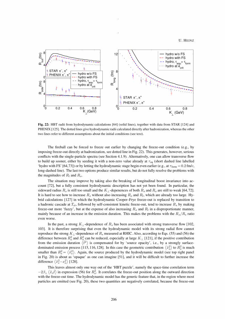
0

4

8

Rou

t(fm)

STAR π−, π+

PHENIX π−, π+

0 0.2 0.4 0.6 0.80

4

8

Rsi

de(fm

)

K⊥(GeV)

hydro w/o FShydro with FShydro, τ

equ= τ

formhydro at e

crit

0 0.2 0.4 0.6 0.80

4

8

12

K⊥ (GeV)

Rlo

ng (f

m)

STAR π−, π+

PHENIX π−, π+

hydro w/o FShydro with FShydro, τ

equ= τ

formhydro at e

crit

Fig. 22: HBT radii from hydrodynamic calculations [64] (solid lines), together with data from STAR [124] and

PHENIX [125]. The dotted lines give hydrodynamic radii calculated directly after hadronization, whereas the other

two lines refer to different assumptions about the initial conditions (see text).

The fireball can be forced to freeze out earlier by changing the freeze-out condition (e.g., by

imposing freeze-out directly at hadronization, see dotted line in Fig. 22). This generates, however, serious

conflicts with the single-particle spectra (see Section 4.1.9). Alternatively, one can allow transverse flow

to build up sooner, either by seeding it with a non-zero value already at τeq (short dashed line labelled

‘hydro with FS’ [64,73]) or by letting the hydrodynamic stage begin even earlier (e.g., at τ form = 0.2 fm/c,long-dashed line). The last two options produce similar results, but do not fully resolve the problems with

the magnitudes of Rl and Ro.

The situation may improve by taking also the breaking of longitudinal boost invariance into ac-

count [72], but a fully consistent hydrodynamic description has not yet been found. In particular, the

sideward radius Rs is still too small and the K⊥-depenences of both Rs and Ro are still to weak [64,72].

It is hard to see how to increase Rs without also increasing Ro and Rl, which are already too large. Hy-

brid calculations [127] in which the hydrodynamic Cooper–Frye freeze-out is replaced by transition to

a hadronic cascade at Tcr, followed by self-consistent kinetic freeze-out, tend to increase Rs by making

freeze-out more ‘fuzzy’, but at the expense of also increasing Ro and Rl in a disproportionate manner,

mainly because of an increase in the emission duration. This makes the problems with the Ro/Rs ratio

even worse.

In the past, a strong K⊥-dependence of Rs has been associated with strong transverse flow [102,

103]. It is therefore surprising that even the hydrodynamic model with its strong radial flow cannot

reproduce the strong K⊥-dependence of Rs measured at RHIC. Also, according to Eqs. (55) and (56) the

difference between R2o and R2

s can be reduced, especially at large K⊥ [121], if the positive contribution

from the emission duration⟨t2

⟩is compensated for by ‘source opacity’, i.e., by a strongly surface-

dominated emission process [115, 116, 128]. In this case the geometric contribution⟨x2o

⟩to R2

o is much

smaller than R2s =

⟨x2s

⟩. Again, the source produced by the hydrodynamic model (see top right panel

in Fig. 20) is about as ‘opaque’ as one can imagine [51], and it will be difficult to further increase the

difference⟨x2s−x2

o

⟩[128].

This leaves almost only one way out of the ‘HBT puzzle’, namely the space-time correlation term

−2β⊥⟨xot

⟩in expression (56) for R2

o . It correlates the freeze-out position along the outward direction

with the freeze-out time. The hydrodynamic model has the generic feature that, in the region where most

particles are emitted (see Fig. 20), these two quantities are negatively correlated, because the freeze-out

U. HEINZ

206

surface moves from the outside towards the center rather than the other way around. Hence the term

−2β⊥⟨xot

⟩is positive and tends to make R2

o larger than R2s . The small measured ratio Ro/Rs . 1 may

instead call for strong positive xo−t correlations, implying that particles emitted from larger xo values

decouple later. Hydrodynamics can not produce such a positive xo−t correlation (at least not at RHIC

energies). On the other hand, there are indications that microscopic models, such as the AMPT [122]

and MPC [129] models, may produce them, for reasons which are not yet completely understood.

One should also not forget that Fig. 22 really compares two different things: The data are extracted

from the width of the 2-particle correlator in momentum space while in theory one calculates the same

quantities from the source width parameters in coordinate space. The two produce identical results only

for Gaussian sources. The hydrodynamic source functions shown in Figs. 20 and 21 are not very good

Gaussians and show a lot of additional structure. We have checked, however, by explicit computation of

the momentum-space correlation function using Eq. (49) that the non-Gaussian effects are small2. The

largest non-Gaussian effects are seen in the longitudinal radius Rl [112], but although the corresponding

corrections go in the right direction by making the Rl extracted from the momentum-space correlator

smaller, the effect is only a fraction of 1 fm and not large enough to bridge the discrepancy with the data.

It was recently suggested [94, 130] that neglecting dissipative effects might be at the origin of

the discrepancy between the purely hydrodynamic calculations and the data. A calculation of first-order

dissipative corrections to the spectra and HBT radii at freeze-out [94], with a ‘reasonable’ value for the

viscosity, yielded a significant decrease ofRl along with a corresponding strong reduction of the emission

duration contribution to Ro, both as desired by the data. There was no effect on the xo−t correlations,

however, and only a weak effect on Rs which went in the wrong direction, making it even flatter as a

function of K⊥. The rather steep K⊥-dependence of the data for both Rs and Ro and the larger than

predicted size ofRs at lowK⊥ are therefore not explained by this mechanism [94,129]. Furthermore, the

elliptic flow v2 has been shown to be very sensitive to viscosity [94,95], and the viscosity values needed

to produce the desired reduction in Rl turned out [94] to reduce v2 by almost a factor of 2, incompatible

with the data. The RHIC ‘HBT puzzle’ thus still awaits a solution.

5.5 Non-central (b6=0) collisions — azimuthally sensitive HBT interferometry (asHBT)

In non-central collisions the azimuthal symmetry of the source is broken by the impact parameter vector

b which, together with the beam direction, defines the reaction plane. Pairs emitted at different azimuthal

angles Φ =∠(b,K⊥) relative to the reaction plane therefore originate in general from effective emission

regions (homogeneity regions) of different sizes and shapes.

As a result, the components of the spatial correlation tensor Sµν = 〈xµxν〉 now depend not only

on the magnitude of the transverse pair momentum K⊥, but also on its angle Φ relative to the reaction

plane. Furthermore, the source is no longer reflection symmetric with respect to the plane defined by

the beam axis and K⊥ (i.e., symmetric under xs→−xs), so Ros and Rls no longer vanish. This means

that for non-central heavy-ion collisions we have to measure 6 (not 4) HBT radii, and they are functions

not only of Y and K⊥, but also of the emission angle Φ relative to the reaction plane. A complete HBT

analysis of non-central heavy-ion collisions thus requires the event-wise determination of the reaction

plane (through a Fourier analysis of the single-particle spectrum as, for example, used for extracting the

elliptic flow) and the investigation of the dependence of the HBT radii on the angle Φ relative to that

plane.

5.5.1 asHBT formalism

Experimentally it is still useful to characterize the source in terms of HBT radii Ro and Rs parallel and

perpendicular to the transverse emission direction defined by the pair momentum K⊥. The emitting

2They would have been larger if we had included resonance decay pions in the emission function, as found by Lin et

al. [122], which was our main reason for not doing so.


207

source S(x,K), however, is most conveniently written down in transverse coordinates x, y aligned with

the reaction plane, since it typically (at least for collisions between spherical nuclei) is symmetric un-

der reflection with respect to that plane, y→−y combined with Φ→−Φ. The analogue relations to

Eqs. (55)–(57), which express the HBT radii through the components Sµν = 〈xµxν〉, therefore involve

an explicit rotation by the angle Φ between the (x, y) axes characterizing the source Sµν and the (xo, xs)axes defined by the emission direction K⊥ [131–133]:

R2s = 1

2(Sxx+Syy) − 12(Sxx−Syy) cos(2Φ) − Sxy sin(2Φ)

R2o = 1

2(Sxx+Syy) + 12(Sxx−Syy) cos(2Φ) + Sxy sin(2Φ)

−2β⊥(Stx cos Φ+Sty sin Φ) + β2⊥Stt ,

R2os = Sxy cos(2Φ) − 1

2 (Sxx−Syy) sin(2Φ) + β⊥(Stx sin Φ−Sty cos Φ) ,

R2l = Szz − 2βLStz + β2

LStt ,

R2ol = (Sxz−βLStx) cosΦ + (Syz−βLSty) sin Φ − β⊥Stz + βLβ⊥Stt ,

R2sl = (Syz−βLSty) cos Φ − (Sxz−βLStx) sin Φ . (75)

These equations exhibit the explicit Φ-dependence resulting from the rotation between the (x, y) and

(xo, xs) axes, but not the implicit one reflecting the Φ-dependence of the spatial correlation tensor

Sµν(Y,K⊥,Φ). The total emission angle dependence of the HBT radii results from the combination

of both.

The implicit Φ-dependence of the spatial correlation tensor is restricted by symmetries of the

source [133]. It is a relativistic effect associated with an azimuthal spatial source deformation super-

imposed by strong transverse collective flow [131, 134] which vanishes with the fourth power of the

transverse flow velocity v⊥/c for weak or no collective expansion [132, 134].

A full analysis of the symmetry constraints on Sµν(Y,K⊥,Φ) for symmetric collisions between

spherical nuclei and for pairs detected in a symmetric rapidity window around Y = 0 was performed in

Ref. [133]. One finds the following most general form for the azimuthal oscillations of the HBT radii:

R2s = R2

s,0 + 2∑

n=2,4,6,...

R2s,n cos(nΦ) ,

R2os = 2

∑

n=2,4,6,...

R2os,n sin(nΦ) ,

R2o = R2

o,0 + 2∑

n=2,4,6,...

R2o,n cos(nΦ) ,

R2ol = 2

∑

n=1,3,5,...

R2ol,n cos(nΦ) ,

R2l = R2

l,0 + 2∑

n=2,4,6,...

R2l,n cos(nΦ) ,

R2sl = 2

∑

n=1,3,5,...

R2sl,n sin(nΦ) . (76)

We see that only even or odd sine or cosine terms occur, but no mixtures of such terms. Statistical errors

in the resolution of the reaction plane angle, as well as finite angular bin sizes in Φ, tend to reduce the

actually measured oscillation amplitudes; fortunately, these dilution effects can be fully corrected by a

model-independent correction algorithm [133,135]. A Gaussian fit to the thus corrected correlation func-

tion, binned in Y ,K⊥ and emission angle Φ, then yields the ‘true’ HBT radius parameters R2ij(Y,K⊥,Φ)

from which the nth order azimuthal oscillation amplitudes are extracted via

R2ij,n(Y,K⊥) =

1

nbin

nbin∑

j=1

R2ij(Y,K⊥,Φj)osc(nΦj) . (77)

U. HEINZ

208

Here nbin indicates the number of (equally spaced) Φ bins in the data and osc(nΦj) stands for sin(nΦj)or cos(nΦj) as appropriate, see Eqs. (76). (Note that Nyquist’s theorem limits the number of harmonics

that can be extracted to n ≤ nbin.)

We would like to relate the azimuthal oscillation amplitudes of the 6 HBT radius parameters to

the geometric and dynamical anisotropies of the source, as reflected in the azimuthal oscillations of

the 10 independent components of the spatial correlation tensor. Their allowed oscillation patterns at

midrapidity Y = 0 are given by [133]

A(Φ) ≡ 12 〈x2+y2〉 = A0+2

∑n≥2,even An cos(nΦ) ,

B(Φ) ≡ 12 〈x2−y2〉 = B0+2

∑n≥2,even Bn cos(nΦ) ,

C(Φ) ≡ 〈xy〉 = 2∑

n≥2,even Cn sin(nΦ) ,

D(Φ) ≡ 〈t2〉 = D0+2∑

n≥2,even Dn cos(nΦ) ,

E(Φ) ≡ 〈tx〉 = 2∑

n≥1,odd En cos(nΦ) ,

F (Φ) ≡ 〈ty〉 = 2∑

n≥1,odd Fn sin(nΦ) ,

G(Φ) ≡ 〈tz〉 = 2∑

n≥1,odd Gn cos(nΦ) ,

H(Φ) ≡ 〈xz〉 = H0+2∑

n≥2,evenHn cos(nΦ) ,

I(Φ) ≡ 〈yz〉 = 2∑

n≥2,even In cos(nΦ) ,

J(Φ) ≡ 〈z2〉 = J0 +2∑

n≥2,even Jn cos(nΦ) . (78)

The missing terms in the sums over n have amplitudes which are odd functions of Y and vanish at midra-

pidity. They do, however, contribute to the HBT radii if the data are averaged over a finite, symmetric

rapidity window around Y = 0 [133]. Their contributions can be eliminated by varying the width ∆Y of

this rapidity window and extrapolating quadratically to ∆Y → 0. Note that C0 =E0 =F0 =G0 = I0 = 0by symmetry, i.e., the corresponding components of Sµν oscillate around zero.

The oscillation amplitudes of the HBT radii relate to the oscillation amplitudes of the source

parameters as follows [133, 136]: For the odd harmonics n= 1, 3, 5, . . . we have

R2ol,n = 1

2〈Hn−1+Hn+1−In−1+In+1 − βL(En−1+En+1−Fn−1+Fn+1)〉−〈β⊥Gn − βLDn〉 , (79)

R2sl,n = 1

2〈−Hn−1+Hn+1+In−1+In+1 − βL(−En−1+En+1+Fn−1+Fn+1)〉 ,

whereas the even harmonics n = 0, 2, 4, . . . satisfy

R2s,n = 〈An〉 + 1

2〈−Bn−2−Bn+2+Cn−2−Cn+2〉 ,R2o,n = 〈An〉 + 1

2〈Bn−2+Bn+2−Cn−2+Cn+2〉−β⊥〈En−1+En+1−Fn−1+Fn+1〉 + β2

⊥〈Dn〉 ,R2os,n = 1

2〈−Bn−2+Bn+2+Cn−2+Cn+2 + β⊥(En−1−En+1−Fn−1−Fn+1)〉 ,R2l,n = 〈Jn〉 − 2〈βLGn〉 + 〈β2

LDn〉 . (80)

In these relations it is understood that all negative harmonic coefficients n < 0, as well as C0, E0, F0, G0

and I0, are zero. The angular brackets 〈. . . 〉 indicate an average over a finite, symmetric rapidity window

around Y =0. The terms involving the longitudinal pair velocity βL vanish quadratically as the width

∆Y of that window shrinks to zero.

Even after extrapolating to Y = 0 in this way, we still have many more source parameters than

measurable HBT amplitudes. One counts easily that up to n= 2 there are 9 measurable Fourier coef-

ficients which (at Y = 0) depend on 19 source amplitudes. From there on, increasing n by 2 yields 6

additional measured amplitudes which depend on 10 additional source amplitudes. This lack of analysis


209

power is an intrinsic weakness of the HBT microscope and is due to the fundamental restrictions arising

from the mass-shell constraint q0 = β · q. The reconstruction of the source thus must necessarily rely on

additional assumptions.

One such assumption which may not be too unreasonable is that the emission duration D= 〈 t2〉 is

approximately independent of emission angle and that the source is sufficiently smooth that higher order

harmonics n ≥ 3 of Sµν can be neglected. Such source properties would result in the ‘Wiedemann sum

rule’ [131]

R2o,2 −R2

s,2 + 2R2os,2 = 0 , (81)

which can be experimentally tested. If verified for all K⊥ it would provide strong support for the un-

derlying assumptions on the source. In this case we can measure 3 azimuthally averaged HBT radii

and 5 independent oscillation amplitudes with n ≤ 2, depending on 14 source parameters of which 5

can be eliminated by going to K⊥ =β⊥ = 0 (see Ref. [133] for explicit expressions). This makes the

geometry of the effective source for particles with K⊥ = 0 ‘almost solvable’3, as confirmed by hydro-

dynamical calculations [51] which show that at K⊥ = 0 the effective emission region closely tracks the

overall geometry of the source even if it is strongly and anisotropically expanding.

The source geometry can be completely reconstructed from HBT data if transverse flow is so weak

that all implicit Φ-dependence (i.e., all higher harmonics n ≥ 1) of Sµν can be neglected. In this case

one obtains at Y = 0 the ‘geometric relations’ [132]

R2s,0 = A0 = 1

2 〈x2+y2〉0 ,R2o,0 −R2

s,0 = β2⊥D0 = β2

⊥〈t2〉0 ,R2l,0 = J0 = 〈z2〉0 ,

R2ol,1 = −R2

sl,1 = 12H0 = 1

2〈xz〉0 ,R2o,2 = −R2

s,2 = −R2os,2 = 1

2B0 = 14〈x2−y2〉0 . (82)

A0 describes the average transverse size and B0 (which generates a second-order harmonic in the trans-

verse HBT radii) the transverse deformation of the source. H0 generates a first-order harmonic in the oland sl cross terms and describes a longitudinal tilt of the source away from the beam direction [132].

Such a tilt was found in Au+Au collisions at the AGS [138]. Its sign yielded important information on

the kinetic pion production mechanism [132, 138].

5.5.2 Azimuthal oscillations of HBT radii in hydrodynamics and RHIC data

We can use the hydrodynamic model introduced in Section 4.1.9 to describe the momentum spectra

and explore what it would predict for the azimuthal oscillations of the HBT radii in non-central Au+Au

collisions at RHIC [51]. The most interesting question, perhaps, is whether we can reconstruct the

orientation and magnitude of the spatial deformation of the source at freeze-out from the HBT analysis,

thereby complementing our knowledge of the orientation and magnitude of the momentum anisotropy

from the elliptic flow analysis.

To see how different orientations of the spatial deformation (in-plane elongated versus out-of-

plane elongated) manifest themselves in the azimuthal oscillations of the HBT radii, one can explicitly

construct sources of either orientation and perform an HBT analysis on them. Since the elliptic flow

makes the fireball expand faster into the reaction plane than perpendicular to it, we can generate an in-

plane elongated source (IPES) at freeze-out from the initial out-of-plane oriented overlap region simply

3Note that the limit K⊥ → 0 eliminates all influence from the temporal structure of the source. The emission duration and

correlations between position and time at freeze-out must be extracted from correlation data at non-zero K⊥ where, however,

the explicit β⊥-dependence associated with factors t in the variances 〈xµxν〉 interferes with the implicit K⊥-dependence in

the spatial variances which result from collective expansion flow [103]. Models for disentangling these different contributions

to the K⊥-dependence have been extensively studied for azimuthally symmetric sources [103], but must be generalized for

azimuthally deformed sources [137].

U. HEINZ

210

by making sure that the elliptic flow has enough time to act before the system decouples. By increasing

the initial energy density or temperature, we can make the total time until decoupling arbitrarily large.

Let us therefore study hydrodynamic sources evolving from different sets of initial conditions [51].

The first set (labelled ‘RHIC1’) corresponds to optimized values for central Au+Au collisions at√sNN =130 GeV which were used in Section 4.1.9 (see Table 1). The second set of initial conditions

(labelled ‘IPES’) uses a much higher initial temperature Teq = 2 GeV (at b= 0), and the hydrodynamic

evolution is started at τeq = 0.1 fm/c and stopped when a freeze-out temperature Tdec = 100 MeV has been

reached. Such a high initial temperature can probably not even be achieved at the LHC, and the strong

transverse flow generated in this case probably causes the system to decouple already much closer to the

hadronization temperature Tcr = 164 MeV. But if we force the system to start at such a high temperature

and freeze out so low, we give it enough time to convert the initial out-of-plane deformation into a final

in-plane deformation (which is the phenomenon we want to study). The following analysis refers to

semi-peripheral Au+Au collisions with impact parameter b= 7 fm.

Figure 23(a) shows the freeze-out surface tdec(r) in cuts along (y= 0) and perpendicular to the

reaction plane (x= 0). Initially the source is extended out-of-plane (larger in the y- than in the x-

direction), but it then expands more rapidly into the x-direction, becoming in-plane elongated at later

times. For RHIC1 initial conditions this only happens after most of the matter has already decoupled;

as a consequence the time-integrated source, shown in Fig. 23(b), is still longer in the y- than in the

x-direction in the RHIC1 case. For IPES initial conditions the deformation changes sign before most

particles decouple, and the time-integrated source appears in-plane extended [see again Fig. 23(b)]. Also,

it is much larger because of the much higher initial energy density and longer lifetime.

Figure 23(c) shows cuts along and perpendicular to the reaction plane through the density contour

plots d2N/d2r=∫(d3K/EK)dz dt S(x,K) of Fig. 23(b). Pion emission is seen to be strongly surface

peaked, in particular at RHIC1 where the freeze-out radius is almost constant for a long time. This

‘opacity’ is weaker both at lower collision energies (where the freeze-out surface shrinks to zero contin-

uously [50]) and at higher energies, due to larger temporal variations of the freeze-out radius. Figures 24

and 25 show the spatial distributions of pions emitted with fixed momentum. Shown are density contours

of∫dz dt S(x,K) in the transverse plane (x, y) for pions with rapidity Y = 0 and fixed K⊥, for three

emission angles Φ = 0, 45 and 90 relative to the reaction plane. (In Fig. 25 we replaced Φ =45 for

clarity by the equivalent angle Φ =225.) Particles with vanishing transverse momentum K⊥ are seen to

be emitted from almost the entire interior of the ‘bathtub’ shown in Figs. 23(b) and 23(c); for RHIC1 and

IPES initial conditions this region is elongated out-of-plane and in-plane, respectively. For slow pions

the source thus looks transparent. Pions with sufficiently large transverse momenta are emitted from

relatively thin regions close to the rim of the ‘bathtub’ where the flow velocity is largest and points into

the direction of the emitted pions. For fast pions the source thus looks opaque, more so at RHIC than at

higher energies. Their emission regions rotate with the emission angle, constrained by the shape of the

‘bathtub’.

The HBT radii, calculated from the widths of the K-dependent emission regions according to

Eqs. (75), are shown in Fig. 26, as functions of the azimuthal emission angle Φ. (Since Y = 0, all

terms ∼ βL vanish.) Note that R2o and R2

os receive purely geometric and mixed space-time correlation

contributions; the latter are proportional to the pair velocity β⊥. Since we want to use pion interferometry

to obtain information on the geometric deformation of the source at freeze-out, these should be analysed

separately. In the right panel of Fig. 26 we therefore show the geometric contributions separately as thin

circled lines. For a detailed discussion of all the curves in Fig. 26, I refer the reader to Ref. [51]; here I

discuss only the most important point.

Let us first look at the geometric contributions. From Figs. 24 and 25 we already know that

pions with K⊥ = 0 are emitted from almost the entire fireball and thus probe the different sign of the

spatial deformation of the total (momentum-integrated) RHIC1 and IPES sources shown in Fig. 23. This

is reflected by the opposite sign of the oscillation amplitudes of R2s and of the geometric contribution


211

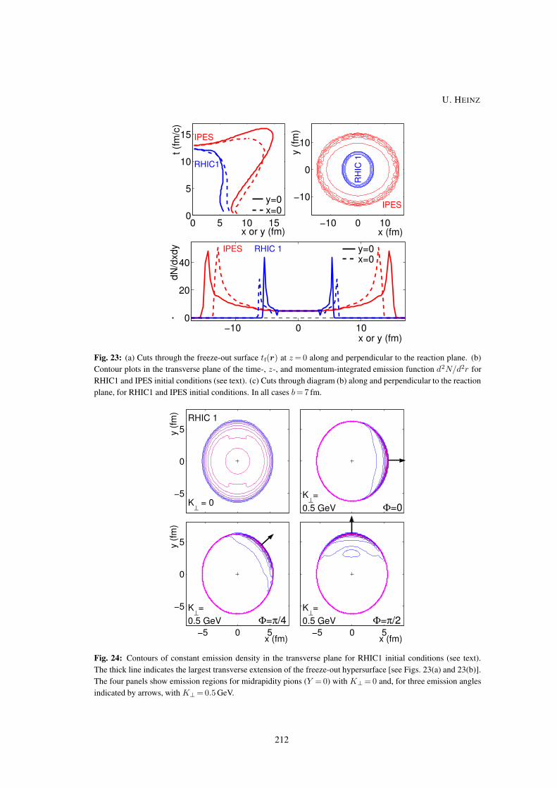
0 5 10 150

5

10

15

x or y (fm)

t (fm

/c)

RHIC1

IPES

y=0x=0

−10 0 10

−10

0

10

x (fm)

y (fm

)

IPES

RH

IC 1

−10 0 100

20

40

x or y (fm)

dN/d

xdy IPES RHIC 1 y=0

x=0

Fig. 23: (a) Cuts through the freeze-out surface tf(r) at z= 0 along and perpendicular to the reaction plane. (b)

Contour plots in the transverse plane of the time-, z-, and momentum-integrated emission function d2N/d2r for

RHIC1 and IPES initial conditions (see text). (c) Cuts through diagram (b) along and perpendicular to the reaction

plane, for RHIC1 and IPES initial conditions. In all cases b=7 fm.

−5

0

5y (fm

)

K⊥ = 0

RHIC 1

K⊥=

0.5 GeV Φ=0

−5 0 5

−5

0

5y (fm

)

x (fm)

K⊥=

0.5 GeV Φ=π/4−5 0 5

x (fm)

K⊥=

0.5 GeV Φ=π/2

Fig. 24: Contours of constant emission density in the transverse plane for RHIC1 initial conditions (see text).

The thick line indicates the largest transverse extension of the freeze-out hypersurface [see Figs. 23(a) and 23(b)].

The four panels show emission regions for midrapidity pions (Y =0) with K⊥ = 0 and, for three emission angles

indicated by arrows, with K⊥ =0.5 GeV.

U. HEINZ

212

−10 0 10

−10

0

10

x (fm)

y (fm

) IPES

K⊥= 0

−10 0 100.5 GeV

x (fm)

K⊥=

Fig. 25: Same as Fig. 24, but for IPES initial conditions

0

5

10

Rsi

de2

(fm

2 )

0

20

40

Rou

t2

(fm

2 )

−1

0

1

0 π/2 πφ

Ros2

(fm

2 )

0

100

200

Rlo

ng2

(fm

2 )

0 π/2 πφ

K⊥ (GeV)

0.000.150.300.45

0

10

20

Rsi

de2

(fm

2 )

0

10

20

30

Rou

t2

(fm

2 )

−1

0

1

0 π/2 πφ

Ros2

(fm

2 )

0

100

200

Rlo

ng2

(fm

2 )

0 π/2 πφ

K⊥ (GeV)

0.000.150.300.45

Fig. 26: Left: Azimuthal oscillations of the HBT radii at Y =0 for b=7 fm Au+Au collisions at√sNN =130 GeV

(RHIC1), for four values of the transverse momentum K⊥ as indicated. Right: The same for IPES initial condi-

tions. For R2o and R2

os the geometric contributions are shown separately as thin circled lines.

to R2o at K⊥ = 0 in the left and right panels of Fig. 26. At higher K⊥ values the oscillations for R2

s

in the right panel of Fig. 26 change sign, but those of the geometric contribution to R2o do not. This

reflects an intricate interplay between geometric and flow effects [51]. However, the opposite signs of

the oscillation amplitudes near K⊥ =0 ofR2s ,R2

o , andR2os for the RHIC1 and IPES sources are clear and

unique indicators of the opposite directions of the spatial deformation for these two sources and can thus

be used to diagnose the latter. In particular, the ratio of the second harmonic oscillation amplitude R2s,2

of the sideward radius to its Φ-averaged value R2s,0 is seen to be almost independent of K⊥ [51, 137].

This ratio can therefore be used to extract the spatial deformation of the entire source even at non-zero

(albeit not too large) K⊥, even though the homogeneity regions at non-zero K⊥ do not probe the entire

source [137, 139].

Recently, the STAR collaboration published the first azimuthally sensitive HBT analysis of Au+Au

collisions at RHIC [139]. As you can see in Fig. 27, the quality and level of detail of the data is impres-

sive. The analysis is fully three-dimensional in the relative momentum q and sufficiently finely binned

in K⊥, Φ, and collision centrality to obtain a reasonably complete HBT snapshot of the final state of the

collision fireball created at RHIC. (Of course, theorists will always keep asking for more detail, but even


213

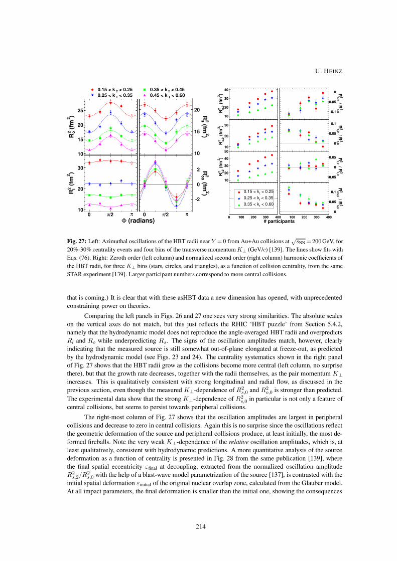
)2 (

fm2 o

R

10

15

20

25

)2

(fm

2 lR

10

20

30

) 2 (fm

2sR

10

15

20

) 2 (fm

2os

R

-2

0

2

0 /2π π 0 /2π π

< 0.25T0.15 < k < 0.35T0.25 < k

< 0.45T0.35 < k < 0.60T0.45 < k

(radians)Φ

< 0.25t0.15 < k < 0.35t0.25 < k < 0.60t0.35 < k

)2

(fm

2 o,0

R

10

20

30

40

)2

(fm

2 s,0

R

10

20

30

)2 (

fm2 l,0

R

10

20

30

40

50

2s,0

/ R2o

,2R

-0.1

-0.05

0

2s,0

/ R2s

,2R

0

0.05

0.1

2l,0 / R

2l,2R

-0.05

0

0.05

2s,0

/ R2o

s,2

R

0

0.05

0.1

0 100 200 300 4000 100 200 300 400

# participants

Fig. 27: Left: Azimuthal oscillations of the HBT radii near Y = 0 from Au+Au collisions at√sNN =200 GeV, for

20%-30% centrality events and four bins of the transverse momentumK⊥ (GeV/c) [139]. The lines show fits with

Eqs. (76). Right: Zeroth order (left column) and normalized second order (right column) harmonic coefficients of

the HBT radii, for three K⊥ bins (stars, circles, and triangles), as a function of collision centrality, from the same

STAR experiment [139]. Larger participant numbers correspond to more central collisions.

that is coming.) It is clear that with these asHBT data a new dimension has opened, with unprecedented

constraining power on theories.

Comparing the left panels in Figs. 26 and 27 one sees very strong similarities. The absolute scales

on the vertical axes do not match, but this just reflects the RHIC ‘HBT puzzle’ from Section 5.4.2,

namely that the hydrodynamic model does not reproduce the angle-averaged HBT radii and overpredicts

Rl and Ro while underpredicting Rs. The signs of the oscillation amplitudes match, however, clearly

indicating that the measured source is still somewhat out-of-plane elongated at freeze-out, as predicted

by the hydrodynamic model (see Figs. 23 and 24). The centrality systematics shown in the right panel

of Fig. 27 shows that the HBT radii grow as the collisions become more central (left column, no surprise

there), but that the growth rate decreases, together with the radii themselves, as the pair momentum K⊥increases. This is qualitatively consistent with strong longitudinal and radial flow, as discussed in the

previous section, even though the measured K⊥-dependence of R2s,0 and R2

o,0 is stronger than predicted.

The experimental data show that the strong K⊥-dependence of R2s,0 in particular is not only a feature of

central collisions, but seems to persist towards peripheral collisions.

The right-most column of Fig. 27 shows that the oscillation amplitudes are largest in peripheral

collisions and decrease to zero in central collisions. Again this is no surprise since the oscillations reflect

the geometric deformation of the source and peripheral collisions produce, at least initially, the most de-

formed fireballs. Note the very weak K⊥-dependence of the relative oscillation amplitudes, which is, at

least qualitatively, consistent with hydrodynamic predictions. A more quantitative analysis of the source

deformation as a function of centrality is presented in Fig. 28 from the same publication [139], where

the final spatial eccentricity εfinal at decoupling, extracted from the normalized oscillation amplitude

R2s,2/R

2s,0 with the help of a blast-wave model parametrization of the source [137], is contrasted with the

initial spatial deformation εinitial of the original nuclear overlap zone, calculated from the Glauber model.

At all impact parameters, the final deformation is smaller than the initial one, showing the consequences

U. HEINZ

214

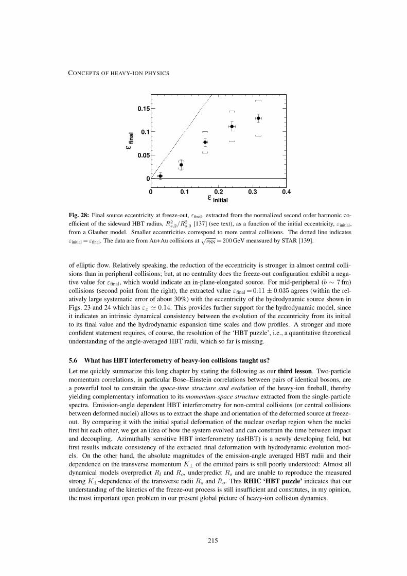
0 0.1 0.2 0.3 0.4

0

0.05

0.1

0.15

initialε

fin

al

ε

Fig. 28: Final source eccentricity at freeze-out, εfinal, extracted from the normalized second order harmonic co-

efficient of the sideward HBT radius, R2s,2/R

2s,0 [137] (see text), as a function of the initial eccentricity, εinitial,

from a Glauber model. Smaller eccentricities correspond to more central collisions. The dotted line indicates

εinitial = εfinal. The data are from Au+Au collisions at√sNN =200 GeV meassured by STAR [139].

of elliptic flow. Relatively speaking, the reduction of the eccentricity is stronger in almost central colli-

sions than in peripheral collisions; but, at no centrality does the freeze-out configuration exhibit a nega-

tive value for εfinal, which would indicate an in-plane-elongated source. For mid-peripheral (b ∼ 7 fm)

collisions (second point from the right), the extracted value εfinal =0.11 ± 0.035 agrees (within the rel-

atively large systematic error of about 30%) with the eccentricity of the hydrodynamic source shown in

Figs. 23 and 24 which has εx ' 0.14. This provides further support for the hydrodynamic model, since

it indicates an intrinsic dynamical consistency between the evolution of the eccentricity from its initial

to its final value and the hydrodynamic expansion time scales and flow profiles. A stronger and more

confident statement requires, of course, the resolution of the ‘HBT puzzle’, i.e., a quantitative theoretical

understanding of the angle-averaged HBT radii, which so far is missing.

5.6 What has HBT interferometry of heavy-ion collisions taught us?

Let me quickly summarize this long chapter by stating the following as our third lesson. Two-particle

momentum correlations, in particular Bose–Einstein correlations between pairs of identical bosons, are

a powerful tool to constrain the space-time structure and evolution of the heavy-ion fireball, thereby

yielding complementary information to its momentum-space structure extracted from the single-particle

spectra. Emission-angle dependent HBT interferometry for non-central collisions (or central collisions

between deformed nuclei) allows us to extract the shape and orientation of the deformed source at freeze-

out. By comparing it with the initial spatial deformation of the nuclear overlap region when the nuclei

first hit each other, we get an idea of how the system evolved and can constrain the time between impact

and decoupling. Azimuthally sensitive HBT interferometry (asHBT) is a newly developing field, but

first results indicate consistency of the extracted final deformation with hydrodynamic evolution mod-

els. On the other hand, the absolute magnitudes of the emission-angle averaged HBT radii and their

dependence on the transverse momentum K⊥ of the emitted pairs is still poorly understood: Almost all

dynamical models overpredict Rl and Ro, underpredict Rs and are unable to reproduce the measured

strong K⊥-dependence of the transverse radii Rs and Ro. This RHIC ‘HBT puzzle’ indicates that our

understanding of the kinetics of the freeze-out process is still insufficient and constitutes, in my opinion,

the most important open problem in our present global picture of heavy-ion collision dynamics.


215

6 Statistical hadronization and primordial hadrosynthesis

In this section we will discuss the kind of information that can be extracted from the measured hadron

abundances (i.e., from the normalization of the hadron spectra, in contrast to their shape which we

discussed in the previous section). Up to this point we did not discuss the normalization of any of

the spectra, nor did we care about it. All we needed for local thermal equilibrium and the build-up of

thermal pressure and collective flow was rapid momentum equilibration, and this can in principle be

achieved entirely by elastic collisions (including resonant elastic collisions in the hadronic phase such

as π+N → ∆ → π+N ) which do not change any of the particle abundances. Whether or not the

microscopic interactions alter the chemical composition or leave it unchanged is, for this part of the

discussion, entirely irrelevant.

This analysis of the spectral shapes has already taught us that hadrons are not formed right away

but appear with some delay via the hadronization of a dense, thermalized, collectively expanding quark–

gluon system. Let us now consider this hadronization process and ask how it affects the hadron abun-

dances, i.e., the chemical composition of the hadronic system emerging from this process.

6.1 Statistical hadronization and the Maximum Entropy Principle

The microscopic description of the process in which thousands of quarks and gluons combine to form

thousands of final-state hadrons is clearly an impractical problem. But it is also not needed. A micro-

scopic approach is called for if we want to understand the (relatively rare) processes by which, say, a

high-p⊥ hadron of a given flavour is created. Such particles probe the microscopic dynamics of high-p⊥parton production, which is controlled by QCD, and although they may rescatter in the dense fireball

medium they never completely lose their memory of the primary production process. We can exploit this

and use them as ‘deep probes’ for the fireball matter, but extracting the information on their production

and subsequent medium modification then clearly requires a detailed microscopic treatment, including

the hadronization of such hard partons. This is completely different for soft partons and hadrons: in

their case the rescattering by the medium wipes out all memories of their initial production process, and

there is no way their final momenta could ever be traced back to their initial momenta. This is in partic-

ular true for the hadronization process, which is probably the most non-perturbative process imaginable:

there are literally innumerable different microscopic channels which might lead to the production of, say,

a negative pion with a soft momentum of order 300 MeV/c in the laboratory.

The proper approach to such a non-perturbative, multi-channel multi-particle problem is (as al-

ready recognized by Fermi, Landau and Hagedorn more than half a century ago) a statistical one. From

a microscopic point of view, there is really very little information we can extract from the yields and

momentum spectra of soft single hadrons. Owing to the strong interactions among the quarks and gluons

as they are forming hadrons, anything that is not explicitly forbidden by the conservation laws for energy,

momentum, baryon number, electric charge, and net strangeness will in fact happen. (Net strangeness

can only be changed by weak interactions, on a time scale which is much too long compared with that of

a heavy-ion collision.)

Note that such a statistical approach has, of course, its limitations: when we start to investigate

correlations between pairs, triplets, quadruplets, etc. of particles, at some level they will begin to realize

that they all belong to a single heavy-ion collision event and are not produced entirely inependently,

but correlated in a non-statistical way. (For example, the momenta of all 2,479 particles emerging from

the collision have to add up to the total momentum of the initially colliding nuclei, and this is likely

to generate non-statistical momentum correlations among considerably smaller subclusters of particles.)

The statistical approach is certainly best justified for single-particle observables, such as hadron spectra

and abundances.

These words are translated into equations via the Maximum Entropy Principle [140].

U. HEINZ

216

Let us consider the entropy S of a small fluid cell of size ∆V in its own rest system,

S = −∑

k

∫

∆V

∫d3x d3p

(2π)3

[fi ln fi + ϑi

(1 − ϑifi

)ln

(1 − ϑifi

)], (83)

where the sum over i includes all particle species in the cell and ϑi= + 1 and −1 for fermions and

bosons, respectively. We assume that soft hadronization happens through many different channels which

are constrained only by the local (in ∆V ) conservation laws for energy, baryon number and strangeness

(∫dω =

∫∆V

∫ d3xd3p(2π)3

):

〈E〉 =

∫dω

∑

i

Eifi , 〈B〉 =

∫dω

∑

i

Bifi , 〈S〉 =

∫dω

∑

i

Sifi = 0 . (84)

Here Bi and Si are the baryon number and strangeness carried by each particle of species i, and we used

the fact that the net strangeness of the two colliding nuclei is zero and that strong interactions keep it

that way locally. Maximizing S with these constraints gives for the most likely distribution for particle

species i [141]

fi(Ei,∆V ) =1

eβ(∆V )[Ei−µi(∆V )] + ϑiwith µi(∆V ) = BiµB(∆V ) + SiµS(∆V ) , (85)

where β, µB and µS are Lagrange multipliers related to the values of the constraints (84) in ∆V . If

the hadronization process does not change the number of ss pairs (for example, because strange valence

quarks are too heavy), we should implement an additional constraint on the total number of strange

quarks and antiquarks which fixes that number to the value before hadronization begins. In this case the

expression for µi in (85) generalizes to µi=BiµB + SiµS + |si|µs where |si| is the total number of

strange quarks and antiquarks in hadron i and µs is a further Lagrange multiplier related to this additional

constraint. The associated fugacity γs = eβµs is known as the ‘strangeness saturation factor’ [142]. An

undersaturation of the strange particle phase space relative to its chemical equilibrium value corresponds

to γs< 1, and an oversaturation to γs> 1.

Equation (85) is a local thermal and chemical equilibrium distribution function. If the system could

be kept at constant volume, any type of strong interaction among the hadrons would leave this distribution

unchanged since such microscopic processes again conserve energy, baryon number and strangeness.

However, the apparent ‘equilibrium’ expressed by Eq. (85) is not achieved kinetically (i.e., as a result of

hadronic rescattering) but statistically (by interference of many different hadron production channels). It

does not require a thermalized prehadronic state (although very strong deviations from equilibrium, e.g.,

at high p⊥, in the prehadronic state may survive the hadronization process and invalidate the Maximum

Entropy Principle).

It is very important to realize that the same local equilibrium distribution (85) can be the result of

two conceptually entirely different types of process. We can take a system of hadrons with an arbitrary

(except for the constraint on total energy, baryon number and strangeness) initial phase-space distribu-

tion and let it evolve for a sufficiently long time to obtain Eq. (85) as a result of the action of elastic

and inelastic processes among the hadrons. This is kinetic equilibration. Or we can produce a system

of hadrons of given energy, baryon number and strangeness from some non-hadronic state by a statis-

tical process which fills hadronic phase-space in the statistically most probable configuration. This is

statistical equilibrium. Both processes share the property that they lead to a state of Maximum Entropy.

However, statistical hadronization can produce a Maximum Entropy distribution through non-hadronic

processes which occur much faster than any inelastic scattering among hadrons at the given energy and

baryon number density.

If you try to create, via statistical hadronization, a ‘pre-established equilibrium’ distribution (85) of

hadrons at energy density e> ecr (T >Tcr), lattice QCD tells us that such a ‘superheated’ hadronic equi-

librium configuration is unstable against deconfinement. If you leave this system to itself, the hadrons


217

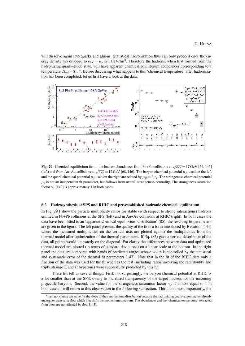
will dissolve again into quarks and gluons. Statistical hadronization thus can only proceed once the en-

ergy density has dropped to ehad = ecr ' 1 GeV/fm3. Therefore the hadrons, when first formed from the

hadronizing quark–gluon state, will have apparent chemical equilibrium abundances corresponding to a

temperature Thad =Tcr4. Before discussing what happens to this ‘chemical temperature’ after hadroniza-

tion has been completed, let us first have a look at the data.

10-1

1

10

10 2

10 3

10-1

1 10 102

Multiplicity (therm. model)

Mul

tiplic

ity (d

ata)

SpS Pb+Pb collisions 158A GeV/c

T=158.8±1.6 MeV

µB=244.7±5.5 MeV

γs=0.821±0.024

χ2=23.5/10 dof

πBK+

K0

K-

Λ

φp–

Λ–

Ξ-

Ξ–+Ω-

Ω–+

Λ(1520)

π+ π- K+ K- K0 p–

Λ Λ* φ Ξ- Ξ–+

Λ–

Ω- Ω–+

B

Res

idua

ls

-5

0

5

0 1 2 3 4 5 6 7 8 9 10 11 12 13 14

Fig. 29: Chemical equilibrium fits to the hadron abundances from Pb+Pb collisions at√sNN =17 GeV [54, 145]

(left) and from Au+Au collisions at√sNN =17 GeV [68, 146]. The baryon chemical potential µB used on the left

and the quark chemical potential µq used on the right are related by µB = 3µq. The strangeness chemical potential

µs is not an independent fit parameter, but follows from overall strangeness neutrality. The strangeness saturation

factor γs [142] is approximately 1 in both cases.

6.2 Hadrosynthesis at SPS and RHIC and pre-established hadronic chemical equilibrium

In Fig. 29 I show the particle multiplicity ratios for stable (with respect to strong interactions) hadrons

emitted in Pb+Pb collisions at the SPS (left) and in Au+Au collisions at RHIC (right). In both cases the

data have been fitted to an ‘apparent chemical equilibrium distribution’ (85); the resulting fit parameters

are given in the figure. The left panel presents the quality of the fit in a form introduced by Becattini [144]

where the measured multiplicities on the vertical axis are plotted against the multiplicities from the

thermal model after optimization of the thermal parameters. If Eq. (85) gave a perfect description of the

data, all points would lie exactly on the diagonal. For clarity the differences between data and optimized

thermal model are plotted (in terms of standard deviations) on a linear scale at the bottom. In the right

panel the data are compared with bands of predicted ranges whose width is controlled by the statistical

and systematic error of the thermal fit parameters [147]. Note that in the fit of the RHIC data only a

fraction of the data was used for the fit whereas the rest (including ratios involving the rare doubly and

triply strange Ξ and Ω hyperons) were successfully predicted by this fit.

These fits tell us several things. First, not surprisingly, the baryon chemical potential at RHIC is

a lot smaller than at the SPS, owing to increased transparency of the target nucleus for the incoming

projectile baryons. Second, the value for the strangeness saturation factor γs is almost equal to 1 in

both cases; I will return to this observation in the following subsection. Third, and most importantly, the

4I am not stating the same for the slope of their momentum distribution because the hadronizing quark–gluon matter already

undergoes transverse flow which blueshifts the momentum spectrum. The abundances and the ‘chemical temperature’ extracted

from them are not affected by flow [143].

U. HEINZ

218

‘chemical decoupling temperature’ Tchem is in both cases much higher than the kinetic freeze-out temper-

ature Tdec extracted from the shape of the momentum spectra. At the SPS Tchem ≈ 160 MeV and at RHIC

Tchem ≈ 175 MeV. Interpreting Tchem in the Maximum Entropy spirit as a Lagrange multiplier which tells

us at which energy density statistical hadronization happened, we see that the data correspond to energy

densities which are very, very close to the critical energy density for deconfinement predicted by lattice

QCD. According to lattice QCD, hadrons in thermodynamic equilibrium cannot exist at temperatures

higher than about 175 MeV if µB = 0, and this limit goes down if µB 6= 0. So these chemical decoupling

temperatures are about as high as they could possibly be for a system of hadrons.

Furthermore, we know from the spectra and elliptic flow that the fireball is collectively expanding

and therefore undergoes rapid cooling. So we face the following conundrum: hadron formation is impos-

sible at energy densities e corresponding to T >Tchem, but once the hadrons are formed at ecr the system

does not remain at this energy density but keeps diluting very rapidly. So if the hadrons first appeared

with arbitrary abundances they would have had no time at all to adjust their abundances to chemical

equilibrium values at Tchem ≈Tcr by inelastic rescattering. The possibility that the measured chemical

freeze-out temperature Tchem ' 160− 170 MeV reflects a kinetically established chemical equilibrium is

therefore logically excluded. The apparent chemical equilibrium at Tchem ≈Tcr seen in the hadron abun-

dances must thus be a ‘pre-established equilibrium’ in the sense of statistical hadronization according to

the Maximum Entropy Principle [15, 148].

0 200 400 600

GeV

0.1

0.2

0.3

0.4

0.5

sπ(dN/dy)

chT

kinT

(a)

η/dchdN0 200 400 600

>β<

0

0.2

0.4

0.6

(b)

η/dchdN

Fig. 30: Left: Pion multiplicity dNπ/dy per unit overlap area S (stars), chemical decoupling temperature Tchem

(circles), and thermal (kinetic) decoupling temperature Tkin (open triangles). Right: Average transverse flow ve-

locity 〈βT〉 at kinetic decoupling as a function of collision centrality (measured by the total charged multiplicity

pseudorapidity density dNchdη at midrapidity) from 200AGeV Au+Au collisions at RHIC [150].

In addition to being logically excluded, there is also strong empirical evidence against a kinetic

interpretation of the observed chemical decoupling temperature. First, it takes the same universal value

of about 170 MeV in high-energy e+e− [144], pp and pp [15], and nucleus–nucleus collisions [149].

Second, in Au+Au collisions at RHIC, Tchem is found to be independent of collision centrality (open

circles in the left panel of Fig. 30), in contrast to the observed significant centrality dependence of the

thermal decoupling temperature and average radial flow velocity extracted from the momentum spectra

(triangles in Fig. 30, see Fig. 9 for comparison and the discussion in Section 4.1.8). As discussed earlier,

any kinetic decoupling process is a competition between local thermalization and global expansion rates.

The latter depends on the size and lifetime of the collision fireball, as reflected by the clear dependence of

the radial flow velocity on the impact parameter of the collision system in the right panel of Fig. 30. The

larger fireballs formed in central collisions live longer, develop more radial flow and cool down to lower

kinetic freeze-out temperatures than the smaller fireballs from more peripheral collisions. The chemical


219

decoupling temperature Tchem, on the other hand, shows no dependence on the collision centrality (size

of the fireball) at all; it can therefore not be controlled by a similar competition between scattering and

expansion as seen in the kinetic decoupling temperature. Tchem and Tkin rest conceptually on different

footings. Tchem is not a kinetic decoupling temperature, but a Lagrange multiplier in the Maximum

Entropy framework whose value indicates the critical energy density at which hadrons are formed.

So if, as we concluded from the momentum spectra, after hadronization the system continues

to expand and cool to lower temperatures, why does not the chemical decoupling temperature Tchem

not follow suit? The answer must be that, after being formed, the hadrons are unable to change their

abundance ratios any further by inelastic rescattering. If this were not the correct interpretation, it would

be very difficult to see how a dozen different hadron species with abundances varying over 3 orders

of magnitude could conspire to look like chemical equilibrium at T ≈Tcr. This would be an unlikely

accident indeed. In Section 6.4 we will see theoretical arguments why chemical decoupling has to happen

more or less directly at Tcr.

6.3 Strangeness enhancement

The fact that the chemical decoupling temperature bears an uncanny resemblance to the predicted phase

transition temperature is, in fact, only half the story. A similar picture of statistical hadronization at

the critical energy density ecr arises even from an analysis of e+e−, pp and pp collisions [15]. What

is really dramatically different in heavy-ion collisions is the level of strangeness saturation reflected in

the apparent chemical equilibrium state. The left panel of Fig. 31 shows that the overall fraction of

0

0.1

0.2

0.3

0.4

0.5

0.6

102

103

√ s (GeV)

λ S

pp collisionspp

– collisions

e+e- collisionsA+B collisions

1

10

0 1 2 3 4 5 6

Strangeness |S|

En

ha

nc

em

en

t E

h-

K0S Λ Λ

–Ξ Ξ

–Ω+Ω

–

0 1 12 2 3

Fig. 31: Left: The strangeness suppression factor of produced strange versus nonstrange quarks,

λs =2 〈ss〉 /⟨

uu+dd⟩

|produced, in elementary particle and heavy-ion collisions as a function of√s [145]. The

two points each for pp collisions reflect the inclusion (exclusion) of the initial valence quarks. Right: Enhance-

ment factor for the midrapidity yields per participating nucleon in 158AGeV/c Pb+Pb relative to p+Pb collisions

for various strange and nonstrange hadron species [151].

strange particles is about twice as high in heavy-ion collisions as in elementary particle collisions! In

other words, strangeness is suppressed relative to its chemical equilibrium saturation value in elemen-

tary particle collisions, but this strangeness suppression has disappeared in A+A collisions. According

to the preceding discussion this extra strangeness cannot have been produced by final state hadronic

rescattering; it thus reflects the properties of the prehadronic state. This points to a new, fast strangeness

production mechanism, either before or during hadronization. Rapid strangeness production from ther-

mal gluons was predicted as one of the key characteristics of a QGP [16].

U. HEINZ

220

A large fraction of the strangeness suppression seen in elementary particle collisions can actually

be understood within the statistical approach. Strong interactions conserve net strangeness exactly, i.e.,

S= 0 without any fluctuations. This means that in principle strangeness conservation should not be

treated in the grand canonical ensemble as in Eqs. (84) and (85), where it is conserved only on average,

but in the canonical ensemble where S is fixed exactly. In the infinite volume limit this makes no differ-

ence, but for the small ‘fireball’ volumes created in elementary particle collisions it is a major correction.

Strange hadrons get suppressed in this way since, together with the strange hadron, a second hadron

with balancing strangeness always has to be created inside the same small volume at the same time, and

this requires more energy. However, even if this canonical effect were the complete explanation of the

suppression in e+e− and pp collisions (which seems quantitatively unlikely [152]), the disappearance of

the effect in heavy-ion collisions would still be most interesting: The absence of canonical strangeness

suppression in nuclear collisions tells us that the creation of a strange hadron at a given position in the

fireball does not require the production of a particle with balancing strangeness nearby (as in pp), but

strangeness can be balanced by production of an antistrange hadron on the other side of the nuclear

fireball. Now we know that all microscopic QCD processes which create ss pairs are local processes,

i.e., the pairs are created at the same point. If the final strange hadron abundances know this no longer,

but behave as if the strange and antistrange hadrons were created independently and statistically dis-

tributed over the entire nuclear fireball, the necessary implication is that they have lost their memory of

the locality of the primary QCD process from which they came and have been able to communicate over

macroscopic fireball distances. I cannot imagine how this is possible without a significant amount of

strangeness diffusion before hadronization.

A very striking way of plotting the ‘strangeness unsuppression’ is shown in the right panel of

Fig. 31 [151]: relative to p+Pb collisions, the number of produced strange hadrons per participating

nucleon is more strongly enhanced the more strange (anti)quarks are required for its formation. For Ω and

Ω this enhancement factor is about 15. The tendency shown in Fig. 31 is completely counterintuitive for

hadronic rescattering mechanisms, where multistrange (anti)baryons are suppressed by higher thresholds

than kaons and Λ’s; but it is perfectly consistent with a statistical hadronization picture [153] where

multistrange particles profit more from the global strangeness enhancement than singly strange hadrons.

6.4 Chemical kinetics after hadronization

The kinetic freeze-out temperatures of about 120 MeV extracted from the hadron momentum spectra tell

us that after hadronization at Tcr ≈ 170 MeV the hadrons continue to rescatter for quite a while. This

rescattering can be simulated in a hadronic cascade such as URQMD [154], using everything that is

known about hadron masses and cross-sections from the Particle Data Tables. These tables tell us that

hadron cross-sections are strongly dominated by resonances at well-defined collision energies, for ex-

ample π+N→∆→π+N , π+π→ ρ→π+π, π+K→K∗ →π+K, etc. These resonances have large

cross sections, hence these types of collision happen frequently and are able to keep up with the collective

expansion of the fireball by continually re-equilibrating the hadron momentum distributions to the falling

temperature. However, almost all of these resonances have the tendency to decay again into exactly the

same hadrons from which they were created (up to charge exchange). The cross-sections for strangeness

exchange processes are considerably smaller, and even smaller are inelastic hadronic processes which

create or annihilate strange quark–antiquark pairs. The resonant collisions thus do not modify the total

measured yields of pions, kaons, and nucleons. For example, the total pion number

N totalπ = Nπ + 2Nρ +N∆ +NK∗ + . . . (86)

is frozen in at Tcr, and similarly for other stable hadrons. This is seen in the bottom part of Fig. 32 which

shows that, if URQMD is initialized with thermodynamic equilibrium abundances and a hydrodynam-

ically generated transverse flow profile similar to the discussion in Section 4, the stable particle yields

hardly change if they are calculated directly at Tcr by simply letting all unstable resonances decay, but

switching off all collisions, or if they are calculated at the end of the entire hadronic cascade.


221

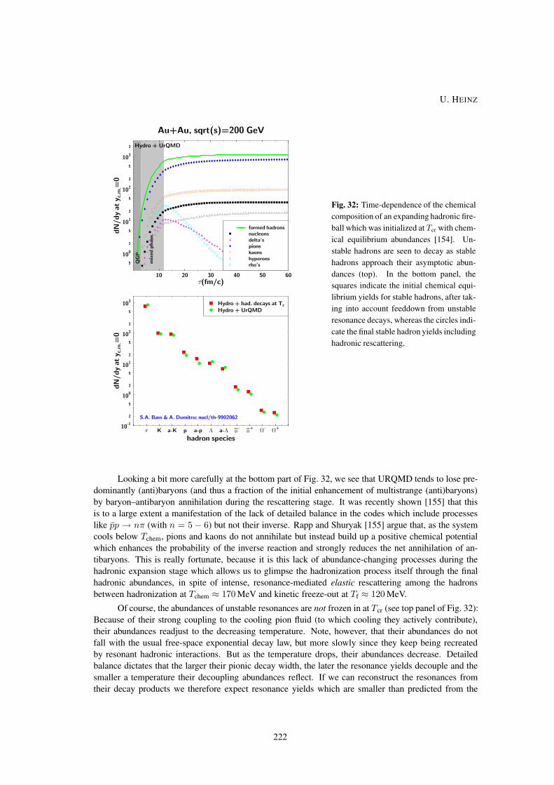
Fig. 32: Time-dependence of the chemical

composition of an expanding hadronic fire-

ball which was initialized at Tcr with chem-

ical equilibrium abundances [154]. Un-

stable hadrons are seen to decay as stable

hadrons approach their asymptotic abun-

dances (top). In the bottom panel, the

squares indicate the initial chemical equi-

librium yields for stable hadrons, after tak-

ing into account feeddown from unstable

resonance decays, whereas the circles indi-

cate the final stable hadron yields including

hadronic rescattering.

Looking a bit more carefully at the bottom part of Fig. 32, we see that URQMD tends to lose pre-

dominantly (anti)baryons (and thus a fraction of the initial enhancement of multistrange (anti)baryons)

by baryon–antibaryon annihilation during the rescattering stage. It was recently shown [155] that this

is to a large extent a manifestation of the lack of detailed balance in the codes which include processes

like pp → nπ (with n = 5 − 6) but not their inverse. Rapp and Shuryak [155] argue that, as the system

cools below Tchem, pions and kaons do not annihilate but instead build up a positive chemical potential

which enhances the probability of the inverse reaction and strongly reduces the net annihilation of an-

tibaryons. This is really fortunate, because it is this lack of abundance-changing processes during the

hadronic expansion stage which allows us to glimpse the hadronization process itself through the final

hadronic abundances, in spite of intense, resonance-mediated elastic rescattering among the hadrons

between hadronization at Tchem ≈ 170 MeV and kinetic freeze-out at Tf ≈ 120 MeV.

Of course, the abundances of unstable resonances are not frozen in at Tcr (see top panel of Fig. 32):

Because of their strong coupling to the cooling pion fluid (to which cooling they actively contribute),

their abundances readjust to the decreasing temperature. Note, however, that their abundances do not

fall with the usual free-space exponential decay law, but more slowly since they keep being recreated

by resonant hadronic interactions. But as the temperature drops, their abundances decrease. Detailed

balance dictates that the larger their pionic decay width, the later the resonance yields decouple and the

smaller a temperature their decoupling abundances reflect. If we can reconstruct the resonances from

their decay products we therefore expect resonance yields which are smaller than predicted from the

U. HEINZ

222

thermal fit of the stable hadron yields:

(K∗

K

)

meas

<

(K∗

K

)

Tchem

, etc. (87)

Such studies are ongoing.

6.5 Primordial hadrosynthesis: measuring the critical temperature for deconfinement

We can summarize the insights gained in this section by stating our fourth lesson: The hadron abun-

dances ‘freeze out’ directly at hadronization. What we see in the SPS and RHIC data are hadron abun-

dances established during primordial hadrosynthesis via a statistical hadronization process. The mea-

sured abundance ratios give for the hadronization temperature Thad ≈Tcr ≈ 170 MeV, confirming pre-

dictions from lattice QCD. The QCD phase transition temperature has thus been measured. This mea-

surement was possible because at SPS and RHIC the fireball expands so rapidly that in the late hadronic

rescattering stage inelastic chemical processes no longer happen. In this way the hadron abundances open

a window onto the hadronization phase transition, even though their momentum distributions continue

to change and cool for several more fm/c.

(MeV)Bµ0 500 1000

T (M

eV)

0

50

100

150

200

250

hadrons

quark gluon plasma

NA49SIS, AGSRHIC

(MeV)Bµ0 500 1000

T (M

eV)

0

50

100

150

200

250

crossoverend

point

Fig. 33: QCD phase diagram with

chemical freeze-out points extracted from

hadron abundance ratios from heavy-ion

(A' 200) collisions at centre-of-mass en-

ergies√sNN ranging from 2.4 to 200 GeV

[54]. The curve and shaded region indi-

cate estimates for the deconfinement phase

transition at finite baryon chemical po-

tential µB from recent lattice QCD cal-

culations [2, 156]. The critical endpoint

where the transition changes from first or-

der (high µB) to continuous crossover (low

µB) is also indicated, although for unre-

alistically large quark masses [2]. (Figure

taken from Ref. [54].)

Figure 33 shows the chemical freeze-out points extracted from hadron yields in A+A collisions

withA' 200, compiled for heavy-ion fixed-target and collider experiments from√sNN ≈ 2.4 GeV (SIS)

to√sNN ≈ 200 GeV (RHIC), and compares them to the latest estimates for the hadronization phase

transition from lattice QCD [2,156]. While for the SPS and RHIC the chemical decoupling temperatures

are consistent with the predicted hadronization temperatures, the values extracted at the Brookhaven AGS

and in particular at the SIS at GSI lie considerably below the phase transition. In these cases statistical

hadronization can not explain the values for Tchem. It is likely that, because of the larger net baryon

densities in lower-energy heavy-ion collisions, inelastic hadronic rescattering processes happen faster

than at higher energies and are able to lead to kinetic readjustment of the chemical temperatue below

Tcr. One should also note, however, that the ‘quality’ of the apparent chemical equilibrium seen at the

AGS and SIS is not as good as at the higher energies since many of the heavier hadrons (in particular

the strange and multistrange antibaryons) are too rare to be measured reliably. The data points labelled

‘SIS, AGS’ in Fig. 33 thus comprise a much smaller number of measured hadron yields, in particular in

the strange sector where only K, K, Λ and ϕ are available at these energies.


223

7 Parton energy loss and jet quenching

In Section 4 we saw that in Au+Au collisions at RHIC the soft momentum particles with p⊥ . 2 GeV/cbehave hydrodynamically. For larger p⊥ the hydrodynamic description gradually breaks down. We

saw this in Section 4.2 when discussing the elliptic flow and how it breaks away from the hydrody-

namically predicted increase with p⊥ above p⊥' 2 GeV/c. In the single-particle spectra the transition

√sNN = 200 GeV

Au+Au, p+p

h++h------------ 2

0 2 4 6 8 10 1210

-10

10-9

10-8

10-7

10-6

10-5

10-4

10-3

10-2

10-1

1

10

102

103

10-7

10-6

10-5

10-4

10-3

10-2

10-1

1

10

102

0-5%5-10% /5 10-20% /10 20-30% /15 30-40% /20 40-60% /25 60-80% /30 p+p (/20 for left axis)

Ed

3NS

D/d

p3(m

b/G

eV

2)

1/(

2πp

T)

d2N

/dp

Td

η| =

0 (

(GeV

/c)-2

)

pT (GeV/c)

Fig. 34: Charged hadron trans-

verse momentum spectra in

pp and Au+Au collisions at√sNN =200 GeV [157]. The

Au+Au data are binned in different

centrality classes as indicated. For

central and semicentral Au+Au

collisions, note the transition

from an exponential behaviour at

p⊥ . 2 GeV/c to a power law for

p⊥> 4 GeV/c.

from collective hydrodynamic behaviour to hard scattering manifests itself by a change of shape: above

p⊥ & 3 − 4 GeV/c the spectra change from a thermal exponential shape to a power law as predicted

by perturbative QCD. Figure 34 shows this for Au+Au collisions at RHIC, together with a comparison

spectrum from pp collisions. This power law affects fewer than 0.1% of all produced hadrons, but it is

these rare high-p⊥ hadrons on which we will focus our attention in this section.

These high-p⊥ hadrons stem from the fragmentation of even-higher-p⊥ partons which, as noted

in Section 3.1, are created very early in the collision, at τform ' 1/p⊥. On their way out of the evolving

collision fireball they interact with the hot matter and probe its properties (density, opacity, etc.). In this

respect they are very similar to positrons in PET (Positron Emission Tomography) where one injects a

positron-emitting source into some living organ and then explores properties of that organ by detecting

these positrons and their energies outside the body. Measuring the properties of hard hadrons emitted

from relativistic heavy-ion collisions thus corresponds to Parton Emission Tomography; but since this

would have the same acronym which might lead to all kinds of confusion, and since we do not really

detect partons but rather their hadronic fragments which form a jet, I follow M. Gyulassy [158] and call

this method JET (for Jet Emission Tomography).

7.1 Radiative energy loss of a fast parton

The idea of jet quenching by parton energy loss goes back to an unpublished preprint by J.D. Bjorken in

1982 [159], but he incorrectly identified elastic parton scattering as the dominant medium interaction by

which the fast parton loses energy. The correct mechanism, namely induced gluon bremsstrahlung, was

identified by Gyulassy and collaborators [160] and first fully evaluated by Baier, Dokshitzer, Mueller,

Peigne, and Schiff [161]. Its quantitative effect on the energy loss has now been calculated by several

groups under various approximations (see Ref. [162] for a recent review).

U. HEINZ

224

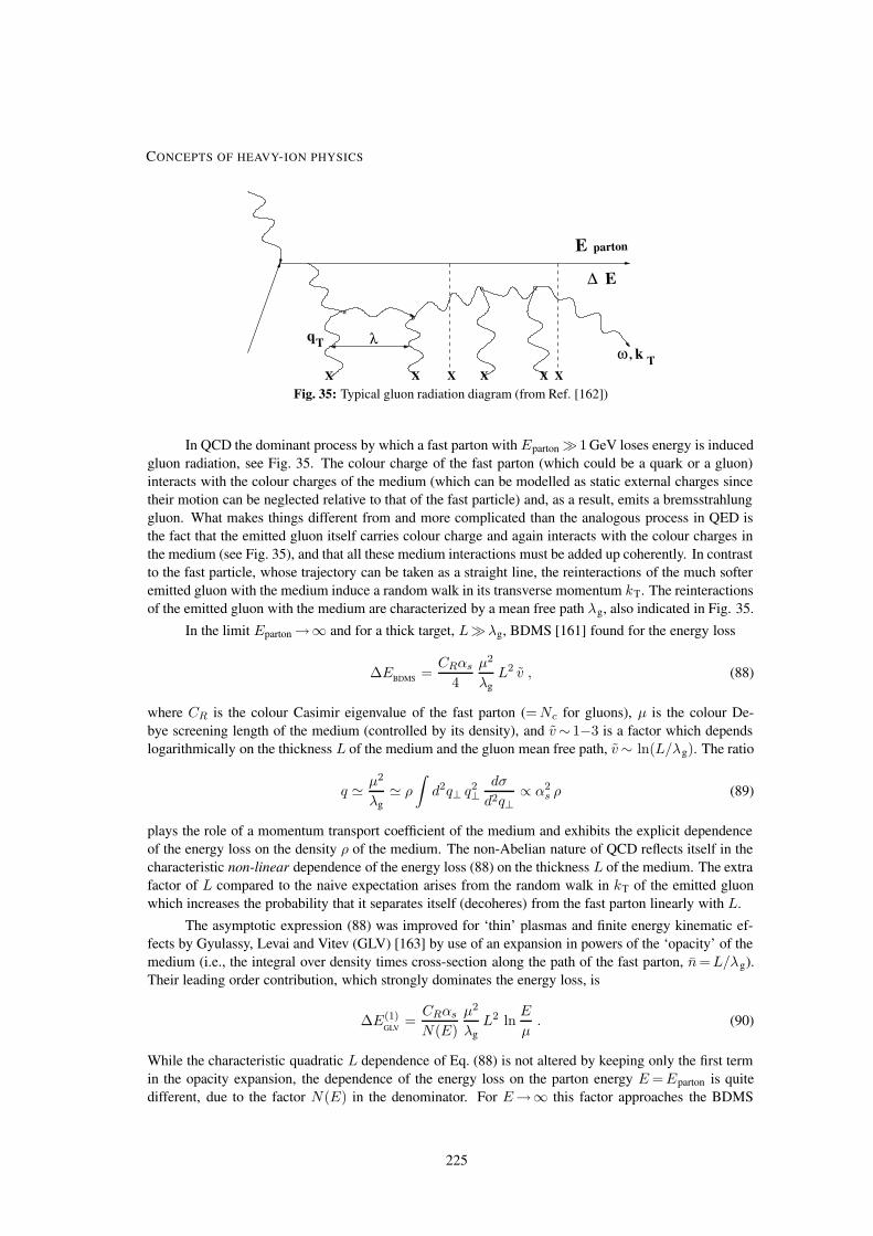
X X X

o

X X X

E parton

ω kλq

T

T,

E∆

oo

Fig. 35: Typical gluon radiation diagram (from Ref. [162])

In QCD the dominant process by which a fast parton with Eparton 1 GeV loses energy is induced

gluon radiation, see Fig. 35. The colour charge of the fast parton (which could be a quark or a gluon)

interacts with the colour charges of the medium (which can be modelled as static external charges since

their motion can be neglected relative to that of the fast particle) and, as a result, emits a bremsstrahlung

gluon. What makes things different from and more complicated than the analogous process in QED is

the fact that the emitted gluon itself carries colour charge and again interacts with the colour charges in

the medium (see Fig. 35), and that all these medium interactions must be added up coherently. In contrast

to the fast particle, whose trajectory can be taken as a straight line, the reinteractions of the much softer

emitted gluon with the medium induce a random walk in its transverse momentum kT. The reinteractions

of the emitted gluon with the medium are characterized by a mean free path λg, also indicated in Fig. 35.

In the limit Eparton →∞ and for a thick target, Lλg, BDMS [161] found for the energy loss

∆EBDMS

=CRαs

4

µ2

λg

L2 v , (88)

where CR is the colour Casimir eigenvalue of the fast parton (=Nc for gluons), µ is the colour De-

bye screening length of the medium (controlled by its density), and v∼ 1−3 is a factor which depends

logarithmically on the thickness L of the medium and the gluon mean free path, v∼ ln(L/λg). The ratio

q ' µ2

λg

' ρ

∫d2q⊥ q

2⊥

dσ

d2q⊥∝ α2

s ρ (89)

plays the role of a momentum transport coefficient of the medium and exhibits the explicit dependence

of the energy loss on the density ρ of the medium. The non-Abelian nature of QCD reflects itself in the

characteristic non-linear dependence of the energy loss (88) on the thickness L of the medium. The extra

factor of L compared to the naive expectation arises from the random walk in kT of the emitted gluon

which increases the probability that it separates itself (decoheres) from the fast parton linearly with L.

The asymptotic expression (88) was improved for ‘thin’ plasmas and finite energy kinematic ef-

fects by Gyulassy, Levai and Vitev (GLV) [163] by use of an expansion in powers of the ‘opacity’ of the

medium (i.e., the integral over density times cross-section along the path of the fast parton, n=L/λg).

Their leading order contribution, which strongly dominates the energy loss, is

∆E(1)GLV

=CRαsN(E)

µ2

λg

L2 lnE

µ. (90)

While the characteristic quadratic L dependence of Eq. (88) is not altered by keeping only the first term

in the opacity expansion, the dependence of the energy loss on the parton energy E=Eparton is quite

different, due to the factor N(E) in the denominator. For E→∞ this factor approaches the BDMS


225

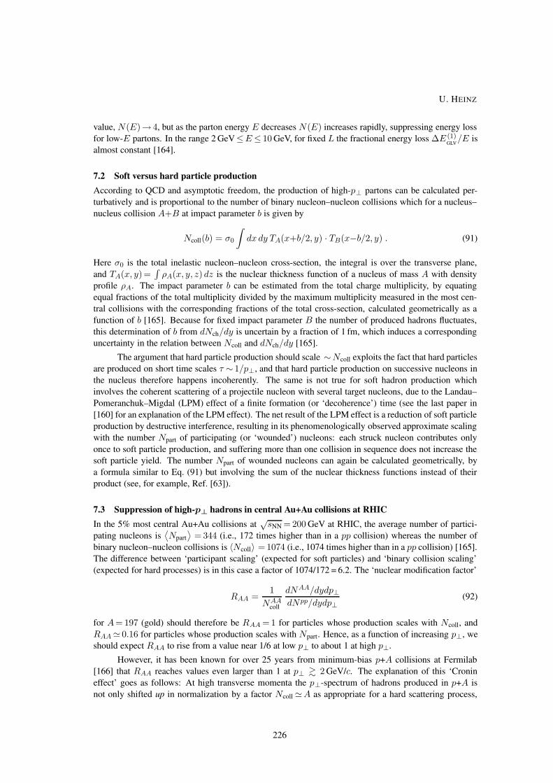
value, N(E)→ 4, but as the parton energy E decreases N(E) increases rapidly, suppressing energy loss

for low-E partons. In the range 2 GeV≤E≤ 10 GeV, for fixed L the fractional energy loss ∆E (1)GLV/E is

almost constant [164].

7.2 Soft versus hard particle production

According to QCD and asymptotic freedom, the production of high-p⊥ partons can be calculated per-

turbatively and is proportional to the number of binary nucleon–nucleon collisions which for a nucleus–

nucleus collision A+B at impact parameter b is given by

Ncoll(b) = σ0

∫dx dy TA(x+b/2, y) · TB(x−b/2, y) . (91)

Here σ0 is the total inelastic nucleon–nucleon cross-section, the integral is over the transverse plane,

and TA(x, y)=∫ρA(x, y, z) dz is the nuclear thickness function of a nucleus of mass A with density

profile ρA. The impact parameter b can be estimated from the total charge multiplicity, by equating

equal fractions of the total multiplicity divided by the maximum multiplicity measured in the most cen-

tral collisions with the corresponding fractions of the total cross-section, calculated geometrically as a

function of b [165]. Because for fixed impact parameter B the number of produced hadrons fluctuates,

this determination of b from dNch/dy is uncertain by a fraction of 1 fm, which induces a corresponding

uncertainty in the relation between Ncoll and dNch/dy [165].

The argument that hard particle production should scale ∼Ncoll exploits the fact that hard particles

are produced on short time scales τ ∼ 1/p⊥, and that hard particle production on successive nucleons in

the nucleus therefore happens incoherently. The same is not true for soft hadron production which

involves the coherent scattering of a projectile nucleon with several target nucleons, due to the Landau–

Pomeranchuk–Migdal (LPM) effect of a finite formation (or ‘decoherence’) time (see the last paper in

[160] for an explanation of the LPM effect). The net result of the LPM effect is a reduction of soft particle

production by destructive interference, resulting in its phenomenologically observed approximate scaling

with the number Npart of participating (or ‘wounded’) nucleons: each struck nucleon contributes only

once to soft particle production, and suffering more than one collision in sequence does not increase the

soft particle yield. The number Npart of wounded nucleons can again be calculated geometrically, by

a formula similar to Eq. (91) but involving the sum of the nuclear thickness functions instead of their

product (see, for example, Ref. [63]).

7.3 Suppression of high-p⊥ hadrons in central Au+Au collisions at RHIC

In the 5% most central Au+Au collisions at√sNN = 200 GeV at RHIC, the average number of partici-

pating nucleons is⟨Npart

⟩= 344 (i.e., 172 times higher than in a pp collision) whereas the number of

binary nucleon–nucleon collisions is 〈Ncoll〉 = 1074 (i.e., 1074 times higher than in a pp collision) [165].

The difference between ‘participant scaling’ (expected for soft particles) and ‘binary collision scaling’

(expected for hard processes) is in this case a factor of 1074/172 = 6.2. The ‘nuclear modification factor’

RAA =1

NAAcoll

dNAA/dydp⊥dNpp/dydp⊥

(92)

for A= 197 (gold) should therefore be RAA = 1 for particles whose production scales with Ncoll, and

RAA' 0.16 for particles whose production scales with Npart. Hence, as a function of increasing p⊥, we

should expect RAA to rise from a value near 1/6 at low p⊥ to about 1 at high p⊥.

However, it has been known for over 25 years from minimum-bias p+A collisions at Fermilab

[166] that RAA reaches values even larger than 1 at p⊥ & 2 GeV/c. The explanation of this ‘Cronin

effect’ goes as follows: At high transverse momenta the p⊥-spectrum of hadrons produced in p+A is

not only shifted up in normalization by a factor Ncoll 'A as appropriate for a hard scattering process,

U. HEINZ

226

but on top of this also horizontally towards higher p⊥ (which at fixed p⊥, of course, manifests itself as

an additional gain, due to the falling nature of the p⊥-spectrum). The horizontal shift towards larger p⊥arises from the fact that the partons inside the projectile nucleon, before making the hard collision which

ends up producing the measured high-p⊥ hadron, already suffer multiple elastic collisions with other

target nucleons which they encounter first, thereby acquiring transverse momentum k⊥ which grows in

a random walk with the square root of the number of these elastic collisions. Once the hard inelastic

collision happens, the projectile parton already brings in this ‘initial k⊥’, thereby giving an extra k⊥kick to the produced hard parton. Since this extra k⊥ is a decreasing fraction of the observed p⊥ as p⊥becomes larger, the Cronin enhancement should disappear as p⊥→∞. (For the same reason the Cronin

effect should become weaker as√sNN increases.) Hence, for large p⊥, RAA should indeed approach the

value 1, not from below due to soft scaling at low p⊥, but rather from above due to Cronin enhancement

at intermediate p⊥ [167]. This behaviour is seen in the two top curves (labelled ‘no dE/dx’) in the right

part of Fig. 36.

(GeV/c)T

p

Ncoll-Scaling

0 2 4 6 8 10

AA

R

0

0.5

1

1.5

2

2.5

3

0-10% central:0π = 200 GeV NNsAu+Au @

= 130 GeV NNsAu+Au @

= 31.0 GeV NNs @ α + α

= 17.3 GeV NNsPb+Pb @

Fig. 36: Left: The nuclear modification ratioRAA defined in Eq. (92) for neutral pions measured in α+α collisions

at the ISR [168], in Pb+Pb collisions at the SPS [169], and in Au+Au collisions at RHIC [170, 171]. (Figure

taken from Ref. [172].) Right: RAA for π0 in central Au+Au collisions at RHIC [170], together with theoretical

calculations [164, 167, 173]. (Figure taken from Ref. [174].)

The left panel of Fig. 36 shows the measured nuclear modification factor for neutral pion pro-

duction in Pb+Pb collisions at the SPS and in Au+Au collisions at RHIC. For comparison also results

from α+α collisions at the ISR in the range 4 GeV/c≤ p⊥≤ 7 GeV/c are included which exhibit the

Cronin effect in this p⊥ region. The Pb+Pb data at√sNN = 17 GeV show a dramatic growth of RAA

with increasing p⊥, starting from participant scaling at low p⊥ but then exceeding the binary collision

limit and exhibiting a strong Cronin enhancement above p⊥ & 2 GeV/c. (This Cronin effect is larger

than in the ISR data, due to both the larger collision system, implying a larger initial k⊥, and the lower

centre-of-mass energy.)

In stark contrast, the RHIC Au+Au data at both 130 and 200 GeV centre-of-mass energy hardly

rise at all above the participant scaling level. With some good will, Rπ0

AA is seen to feature a small

peak around p⊥' 2 GeV RAA, but at a level of less than 50% of the binary collision limit. At higher

p⊥, instead of increasing towards 1, RAA decreases again towards a value of about 0.2. No sign of the

Cronin effect of binary collision scaling anywhere! If we jump ahead to Fig. 37 which shows in the

lower parts of both panels (labelled by ‘Au+Au’) the p⊥-dependence of RAA for all charged particles,

and if we assume that charged and neutral pions (triangles in the left panel) have the same nuclear

modification factor, we see that RAA for heavier charged hadrons must be larger than for pions in the

region 1 GeV/c . p⊥ . 4 GeV/c, but also drop back to well below 1 for p⊥ & 4−5 GeV/c.


227

The conclusion we must draw from these data is that in central Au+Au collisions at RHIC, high-

p⊥ hadron production is suppressed by at least a factor of 5 compared to the perturbative QCD prediction

of binary collision scaling plus Cronin effect (top curves in the right panel of Fig. 36). In fact, looking at

various collision centralities in Au+Au collisions, it was shown explicitly by the PHOBOS collaboration

[175] that above p⊥ & 4 GeV the charged hadron spectra scale again linearly with Npart (i.e., like a soft

process), instead of scaling with Ncoll as expected for a hard process. Furthermore, a crucial control

experiment has recently been completed where the nuclear modification factor was measured in d+Au

collisions (top parts of Fig. 37). One sees that in deuteron–gold collisions RAA =RdAu increases from

(GeV/c)Tp

0 1 2 3 4 5 6 7 8 9 10

AA

R

0

0.2

0.4

0.6

0.8

1

1.2

1.4

1.6

1.8 charged hadronsneutral pions

Au+Au

d+Au

pT (GeV/c)

0 2 4 6 8 100

0.5

1

1.5

2

2.5 d+Au FTPC-Au 0-20%

d+Au Minimum Bias

Au+Au Central

RA

B(p

T)

Fig. 37: The nuclear modification ratioRAA for neutral pions (left) and charged hadrons (left and right), measured

in d+Au and central Au+Au collisions at√sNN = 200 GeV, by PHENIX [176] (left) and by STAR [177] (right).

At intermediate p⊥, 1.5 GeV/c<p⊥< 4 GeV/c, the RAA is systematically larger for charged particles than for π0,

indicating a larger RAA for kaons and protons than for pions in this p⊥-range.

participant scaling at low p⊥ to above 1 at p⊥' 1.5 GeV/c and shows the expected Cronin enhancement

(rather than a suppression) which persists at least up to p⊥ = 8 GeV/c. Again all charged particles taken

together (which includes heavier hadrons such as kaons and protons) show a larger Cronin enhancement

than pions alone (left panel in Fig. 37), and in central d+Au collisions the Cronin effect is a bit larger

than in minimum-bias collisions (right panel in Fig. 37), as expected from the random walk argument for

the initial k⊥.

So the suppression of high-p⊥ hadrons in central Au+Au collisions must be a final state effect

which involves the dense matter created in the heavy-ion collision. It can not be explained as an initial

state effect, i.e., by some property of the internal structure of the gold nucleus which shows up when

probing it at high energies (such as the existence of a ‘colour glass condensate’, see the short discussion

in Section 3.4 and the recent review [28]): Such an effect should still be visible (i.e., some suppression

should persist) if only one of the colliding nuclei is gold [178].

The right panel in Fig. 36 shows that only theories which include an energy loss dE/dx for the fast

partons that produce the high-p⊥ hadrons can account for the RAA data at RHIC. Although the different

theoretical predictions shown in the graph, which use different approximations for the implementation

of the radiative energy loss, give somewhat different p⊥-dependences of RAA and do not agree perfectly

with the data, it is obvious that a significant amount of energy loss is required to account for the observed

suppression by more than a factor of 5 relative to the expected binary collision scaling plus Cronin (upper

curves).

The observed scaling with Npart instead of Ncoll suggests a very interesting geometric interpreta-

tion: Because of the approximately constant density inside an atomic nucleus, the number of participating

U. HEINZ

228

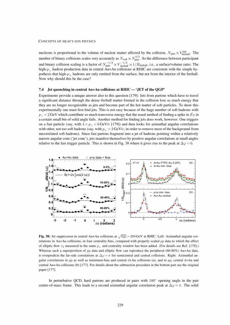
nucleons is proportional to the volume of nuclear matter affected by the collision, Npart ∝V initfireball. The

number of binary collisions scales very accurately asNcoll ∝N4/3part . So the difference between participant

and binary collision scaling is a factor of N−1/3part ∝V

−1/3fireball ∝ 1/Rfireball, i.e., a surface/volume ratio: The

high-p⊥ hadron production data in central Au+Au collisions at RHIC are consistent with the simple hy-

pothesis that high-p⊥ hadrons are only emitted from the surface, but not from the interior of the fireball.

Now why should this be the case?

7.4 Jet quenching in central Au+Au collisions at RHIC — ‘JET of the QGP’

Experiments provide a unique answer also to this question [179]: Jets from partons which have to travel

a significant distance through the dense fireball matter formed in the collision lose so much energy that

they are no longer recognizable as jets and become part of the hot matter of soft particles. To show this

experimentally one must first find jets. This is not easy because of the huge number of soft hadrons with

p⊥< 2 GeV which contribute so much transverse energy that the usual method of finding a spike inET in

a certain small bin of solid angle fails. Another method for finding jets does work, however: One triggers

on a fast particle (say, with 4<p⊥< 6 GeV/c [179]) and then looks for azimuthal angular correlations

with other, not too soft hadrons (say, with p⊥> 2 GeV/c, in order to remove most of the background from

uncorrelated soft hadrons). Since fast partons fragment into a jet of hadrons pointing within a relatively

narrow angular cone (‘jet cone’), jets manifest themselves by positive angular correlations at small angles

relative to the fast trigger particle. This is shown in Fig. 38 where it gives rise to the peak at ∆ϕ= 0.

-3 -2 -1

0

0.2

0.4

0.6

0.8

1

1.2

1.4

1.6

1.8Au+Au data p+p data + flow

))φ∆cos(222

B(1+2v

0-5%

10-20%

30-40%

60-80%

)φ

∆d

N/d

(trigger

1/N

(radians)φ∆0 1 2 3

0

0.1

0.2 d+Au FTPC-Au 0-20%

d+Au min. bias

0

0.1

0.2 p+p min. bias

Au+Au central

1/N

trig

ger d

N/d

(∆φ)

∆φ (radians)0 π/2 π

(a)

(b)

h++h-

Fig. 38: Jet suppression in central Au+Au collisions at√sNN = 200 GeV at RHIC. Left: Azimuthal angular cor-

relations in Au+Au collisions, in four centrality bins, compared with properly scaled pp data to which the effect

of elliptic flow v2 measured in the same p⊥ and centrality window has been added. (For details see Ref. [179].)

Whereas such a superposition of pp data and elliptic flow can reproduce the peripheral (60-80%) Au+Au data,

it overpredicts the far-side correlations at ∆ϕ= π for semicentral and central collisions. Right: Azimuthal an-

gular correlations in pp as well as minimum-bias and central d+Au collisions (a), and in pp, central d+Au and

central Au+Au collisions (b) [177]. For details about the subtraction procedure in the bottom part see the original

paper [177].

In perturbative QCD, hard partons are produced in pairs with 180 opening angle in the pair

centre-of-mass frame. This leads to a second azimuthal angular correlation peak at ∆ϕ=π. The solid


229

histogram in the right panel of Fig. 38 shows this for pp collisions at√sNN =200 GeV [177]. The ‘far-

side’ peak is flatter and wider than the ‘near-side’ peak, due to well-understood trigger effects and a

non-zero probability for semihard gluon emission by one of the two fast partons. Except for a somewhat

higher background from uncorrelated pairs due to increased soft particle production (‘pedestal effect’),

the same pattern is seen in minimum-bias and central d+Au collisions (Fig. 38, upper part of the right

panel).

However, as one goes to Au+Au collisions and moves from peripheral to central collisions (bottom

to top in the left panel of Fig. 38), the away-side peak at ∆ϕ=π disappears. Whatever enhanced angu-

lar correlation survives in almost central Au+Au collisions at ∆ϕ= π is perfectly compatible with the

measured elliptic collective flow v2 in the p⊥-range where the angular correlations are measured [179].

Whereas the far-side jet correlations should be localized in a narrow window of relative pseudorapidity

∆η between the correlated particles, elliptic flow is a global collective effect which is correlated with

the reaction plane and therefore present at both small and large relative pseudorapidity. By subtracting

the correlations for pairs with ∆η > 0.5 from those for pairs with ∆η < 0.5, one in fact completely re-

moves the elliptic flow contribution [179]. For semicentral Au+Au collisions the result of this procedure

is a strongly reduced far-side angular correlation peak, and in central Au+Au collisions it is completely

absent (lower diagram in the right panel of Fig. 38).

Npart

100 150 200 250 300 350

0

0.5

1

1.5

2

100 150 200 250 300 350 4004000 50 50

|∆φ|<0.75|∆φ|>2.24

I AA(∆

φ1,∆

φ2)

Npart

4<pT <6 GeV/ctrig 3<pT

<4 GeV/ctrig

Fig. 39: Left: Suppression of near-side (squares) and far-side (circles) angular correlations in Au+Au collisions

at RHIC, for two different lower p⊥ cuts for the trigger particle [179]. Note the disappearance of the far-side

correlations in central collisions (i.e., for large numbersNpart of participating nucleons). Right: Cartoon illustrating

outward jet emission from the fireball surface and quenching of its inward-moving partner by the dense interior.

One can further quantify this by comparing the area under both near- and far-side peaks of the

azimuthal correlation function (after subtracting elliptic flow) with the corresponding areas in pp colli-

sions. Figure 39 shows the ratio of these areas for the near-side peak as squares and for the far-side peak

as circles. For very peripheral Au+Au collisions both ratios are close to, but slightly less than 1. The

reduction below 1 can be understood as a trigger effect [180]. As the Au+Au collisions become more

central (i.e., Npart increases), the near-side correlations seem to increase, in particular for lower values

of the trigger-p⊥, which may indicate an incomplete subtraction of elliptic flow effects. The away-side

correlations, on the other hand, get weaker in less peripheral collisions and completely vanish in central

collisions. If the elliptic flow were larger than assumed in the subtraction, this would bring down both

the near- and far-side correlation strength, rendering the disappearance of the far-side jets even more

dramatic.

U. HEINZ

230

The interpretation suggested by these data is indicated by the cartoon in the right part of Fig. 39:

The high-p⊥ trigger hadron identifies a jet moving outward from the fireball. The yield of these high-p⊥hadrons scales by a factor N

−1/3part ∝ 1/Rfireball more weakly than expected from perturbation theory, so

these outward-moving jets come only from a thin surface layer. Fast partons created in the interior and

trying to move out, as well as the inward-moving partners of the observed outward-moving jets, lose

so much energy in the dense medium that they no longer make hadrons with p⊥> 2 GeV which are

included in the angular correlation function. (If they still produced hadrons with p⊥> 2 GeV and had

lost no energy but only their angular correlation with the fast trigger particle, the total yield at high p⊥should still scale with Ncoll, i.e., RAA should be 1.)

This amounts to ‘complete jet suppression’: The hot and dense medium (which we know from

Section 4 must be a thermalized QGP) suppresses all jets from fast partons except for a small fraction

being produced near the surface and moving outward. Since in jet fragmentation the leading hadron

carries on average about half the p⊥ of the hard parton, a trigger hadron with a p⊥ between 4 and

6 GeV/c corresponds to p⊥' 10 for both primary partons. The complete disappearance of the far-side

jet in central Au+Au collisions requires the far-side parton to lose at least 6 GeV of momentum such

that its fragments are all below the 2 GeV/c cut imposed on the angular correlation function. The energy

lost by these partons thus becomes part of the thermalized and hydrodynamically expanding medium at

p⊥< 2 GeV/c.

So here is our fifth lesson: The quark–gluon plasma strongly suppresses jets. Inward-moving

partons with p⊥ . 10 GeV do not make it to the opposite edge and become part of the low-p⊥ ‘thermal

soup’. Only outward-moving jets formed near the fireball surface survive. The era of JET (Jet Emission

Tomography) of the QGP has begun: By investigating the A-, b- and emission-angle dependence of

the far-side jet suppression and combining it with information extracted from soft particle emission, we

should be able to accurately determine the fireball conditions (density and temperature) in the early stage.

8 Conclusions and disclaimers

The title of these lectures is ‘Concepts of heavy-ion physics’, but these lecture notes do not give a

comprehensive overview of all the relevant concepts. In 3 × 75 minutes one simply can not cover

everything. Notable omissions include (I give references to good recent reviews) J/ψ suppression [181]

as well as direct photon and thermal dilepton emission [13, 182]. While RHIC has not yet produced

sufficient data on the first two of these items, J/ψ suppression has been a hot subject at the SPS, and some

very interesting signals were also seen in the photon and dilepton spectra [10,183]. I also omitted a more

detailed discussion of the very interesting quark-coalescence approach to the production of hadrons at

intermediate transverse momenta (1.5 GeV/c< p⊥< 6 GeV/c), where some really nice systematics has

been discovered which strongly indicates that in this kinematic region quark counting rules, causing a

meson–baryon splitting of the elliptic flow and hadron yields instead of the hydrodynamic mass splitting

observed at lower p⊥ [184]. I may include a more detailed discussion of these topics in some future

lecture notes.

Relativistic heavy-ion physics is making progress in huge strides. These lectures have taught us

a few important lessons which, I think, are now solidly established; but with the steady stream of RHIC

data Nature is teaching us new, smaller lessons every week which continue to complement the picture

literally as I sit here writing these notes. (Just compare these notes and the many new data I present

here with the copied transparencies distributed at the summer school. And this write-up does not even

mention everything that happened during the last year . . . )


231

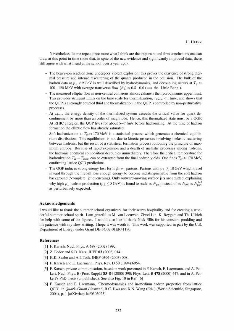
Nevertheless, let me repeat once more what I think are the important and firm conclusions one can

draw at this point in time (note that, in spite of the new evidence and significantly improved data, these

still agree with what I said at the school over a year ago).

– The heavy-ion reaction zone undergoes violent explosion; this proves the existence of strong ther-

mal pressure and intense rescattering of the quanta produced in the collision. The bulk of the

hadron data at p⊥< 2 GeV is well described by hydrodynamics, and decoupling occurs at Tf ≈100−120 MeV with average transverse flow 〈βT〉≈ 0.5−0.6 (=⇒ the ‘Little Bang’).

– The measured elliptic flow in non-central collisions almost exhausts the hydrodynamic upper limit.

This provides stringent limits on the time scale for thermalization, τ therm < 1 fm/c, and shows that

the QGP is a strongly coupled fluid and thermalization in the QGP is controlled by non-perturbative

processes.

– At τtherm the energy density of the thermalized system exceeds the critical value for quark de-

confinement by more than an order of magnitude. Hence, this thermalized state must be a QGP.

At RHIC energies, the QGP lives for about 5−7 fm/c before hadronizing. At the time of hadron

formation the elliptic flow has already saturated.

– Soft hadronization at Tcr ≈ 170 MeV is a statistical process which generates a chemical equilib-

rium distribution. This equilibrium is not due to kinetic processes involving inelastic scattering

between hadrons, but the result of a statistical formation process following the principle of max-

imum entropy. Because of rapid expansion and a dearth of inelastic processes among hadrons,

the hadronic chemical composition decouples immediately. Therefore the critical temperature for

hadronization Tcr =Tchem can be extracted from the final hadron yields. One finds Tcr ≈ 170 MeV,

confirming lattice QCD predictions.

– The QGP induces strong energy loss for high-p⊥ partons. Partons with p⊥ . 10 GeV which travel

inward through the fireball lose enough energy to become indistinguishable from the soft hadron

background (‘complete’ jet quenching). Only outward-moving surface jets are emitted, explaining

why high-p⊥ hadron production (p⊥ ≤ 8 GeV) is found to scale ∝Npart instead of ∝Ncoll ∝N4/3part

as perturbatively expected.

Acknowledgements

I would like to thank the summer school organizers for their warm hospitality and for creating a won-

derful summer school spirit. I am grateful to M. van Leeuwen, Ziwei Lin, K. Reygers and Th. Ullrich

for help with some of the figures. I would also like to thank Nick Ellis for his constant prodding and

his patience with my slow writing. I hope it was worth it. This work was supported in part by the U.S.

Department of Energy under Grant DE-FG02-01ER41190.

References

[1] F. Karsch, Nucl. Phys. A 698 (2002) 199c.

[2] Z. Fodor and S.D. Katz, JHEP 03 (2002) 014.

[3] K.K. Szabo and A.I. Toth, JHEP 0306 (2003) 008.

[4] F. Karsch and E. Laermann, Phys. Rev. D 50 (1994) 6954.

[5] F. Karsch, private communication, based on work presented in F. Karsch, E. Laermann, and A. Pei-

kert, Nucl. Phys. B (Proc. Suppl.) 83–84 (2000) 390; Phys. Lett. B 478 (2000) 447; and in A. Pei-

kert’s PhD thesis (unpublished). See also Fig. 10 in Ref. [6]

[6] F. Karsch and E. Laermann, ‘Thermodynamics and in-medium hadron properties from lattice

QCD’, in Quark–Gluon Plasma 3, R.C. Hwa and X.N. Wang (Eds.) (World Scientific, Singapore,

2004), p. 1 [arXiv:hep-lat/0305025].

U. HEINZ

232

[7] U. Heinz, P.R. Subramanian, H. Stocker, and W. Greiner, J. Phys. G 12 (1986) 1237.

[8] K. Rajagopal, Comments Nucl. Part. Phys. A 2 (2002) 120 [arXiv:hep-ph/0009058].

[9] D.H. Rischke, Prog. Part. Nucl. Phys. 52 (2004) 197.

[10] see http://cern.web.cern.ch/CERN/Announcements/2000/NewStateMatter/ and U. Heinz, M. Ja-

cob, arXiv:nucl-th/0002042.

[11] M. Gyulassy, I. Vitev, X.N. Wang, and B.W. Zhang, ‘Jet quenching and radiative energy loss

in dense nuclear matter’, in Quark–Gluon Plasma 3, R.C. Hwa and X.N. Wang (Eds.) (World

Scientific, Singapore, 2004), p. 123 [arXiv:nucl-th/0302077].

[12] T. Matsui and H. Satz, Phys. Lett. B 178 (1986) 416.

[13] P.V. Ruuskanen, ‘Photons and lepton pairs: The deep probes of quark–gluon plasma’, in: Particle

Production in Highly Excited Matter, H.H. Gutbrod and J. Rafelski (Eds.), NATO ASI Series B:

Physics Vol. 303 (1993) 593 (Plenum, New York).

[14] R. Hagedorn, Nuovo Cim. Suppl. 3 (1965) 147.

[15] F. Becattini and U. Heinz, Z. Phys. C 76 (1997) 269.

[16] J. Rafelski and B. Muller, Phys. Rev. Lett. 48 (1982) 1066, Erratum ibid. 56 (1986) 2334.

[17] J. Rafelski, Phys. Rep. 88 (1982) 331.

[18] E. Schnedermann, Z. Phys. C 64 (1994) 85.

[19] J. Sollfrank, P. Koch, and U. Heinz, Z. Phys. C 52 (1991) 593.

[20] E. Schnedermann, J. Sollfrank, and U. Heinz, Phys. Rev. C 48 (1993) 2462.

[21] K.J. Eskola, K. Kajantie, and J. Lindfors, Nucl. Phys. B 323 (1989) 37.

[22] K.J. Eskola, K. Kajantie, P.V. Ruuskanen, and K. Tuominen, Nucl. Phys. B 570 (2000) 379.

[23] B. Andersson, G. Gustafson, G. Ingelman, and T. Sjostrand, Phys. Rep. 97 (1983) 31.

[24] L.V. Gribov, E.M. Levin, and M.G. Ryskin, Phys. Rep. 100 (1983) 1.

[25] A.H. Mueller and J.W. Qiu, Nucl. Phys. B 268 (1986) 427.

[26] L.D. McLerran and R. Venugopalan, Phys. Rev. D 49 (1994) 2233 and 3352.

[27] Y.V. Kovchegov and A.H. Mueller, Nucl. Phys. B 529 (1998) 451.

[28] E. Iancu, A. Leonidov, and L. McLerran, ‘The colour glass condensate: An introduction’, in QCD

perspectives on hot and dense matter, J.-P. Blaizot and E. Iancu (Eds.), NATO Science Series II:

Mathematics, Physics, and Chemistry, Vol. 87 (2002) 73 (Kluwer, Dordrecht, The Netherlands)

[arXiv:hep-ph/0202270].

[29] Y.V. Kovchegov, Nucl. Phys. A 692 (2001) 557.

[30] K. Geiger, Phys. Rep. 258 (1995) 237.

[31] D. Molnar and M. Gyulassy, Phys. Rev. C 62 (2000) 054907.

[32] H.T. Elze and U. Heinz, Phys. Rep. 183 (1989) 81.

[33] R. Baier, A.H. Mueller, D. Schiff, and D.T. Son, Phys. Lett. B 502 (2001) 51.

[34] A.H. Mueller and D.T. Son, Phys. Lett. B 582 (2004) 279.

[35] S. Jeon, Phys. Rev. D 52 (1995) 3591.

[36] P. Arnold, G.D. Moore, and L.G. Yaffe, JHEP 0305 (2003) 051.

[37] G. Aarts and J.M. Martinez Resco, Phys. Rev. D 68 (2003) 085009.

[38] S.A. Bass et al., Phys. Rev. C 60 (1999) 021902.

[39] D. Teaney, J. Lauret, and E.V. Shuryak, arXiv:nucl-th/0110037.

[40] D. Teaney, J. Lauret, and E.V. Shuryak, Nucl. Phys. A 698 (2002) 479.

[41] J.D. Bjorken, Phys. Rev. D 27 (1983) 140.

[42] F. Cooper and G. Frye, Phys. Rev. D 10 (1974) 186.

[43] P.V. Ruuskanen, Acta Phys. Pol. 18 (1987) 551.


233

[44] U. Heinz, K.S. Lee, and E. Schnedermann, ‘Hadronization of a Quark–Gluon Plasma’, in Quark–

Gluon Plasma, R.C. Hwa (Ed.) (World Scientific, Singapore, 1990), p. 471.

[45] K.S. Lee, U. Heinz, and E. Schnedermann, Z. Phys. C 48 (1990) 525.

[46] T. Peitzmann, Eur. Phys. J. C 26 (2003) 539.

[47] E. Schnedermann, J. Sollfrank, and U. Heinz, ‘Fireball spectra’, in: Particle production in highly

excited matter, H.H. Gutbrod and J. Rafelski (Eds.), NATO Asi Series B Vol. 303 (1993) 175

(Plenum Press, New York).

[48] U. Mayer and U. Heinz, Phys. Rev. C 56 (1997) 439.

[49] E. Schnedermann and U. Heinz, Phys. Rev. C 50 (1994) 1675.

[50] P.F. Kolb, J. Sollfrank, and U. Heinz, Phys. Lett. B 459 (1999) 667.

[51] U. Heinz and P.F. Kolb, Phys. Lett. B 542 (2002) 216.

[52] P.J. Siemens and J.O. Rasmussen, Phys. Rev. Lett. 42 (1979) 880.

[53] R. Scheibl and U. Heinz, Phys. Rev. C 59 (1999) 1585.

[54] M. van Leeuwen et al. (NA49 Collab.), Nucl. Phys. A 715 (2003) 161c.

[55] O. Barannikova, F. Wang et al. (STAR Collaboration), Nucl. Phys. A 715 (2003) 458c.

[56] J.M. Burward-Hoy et al. (PHENIX Collaboration), Nucl. Phys. A 715 (2003) 498c.

[57] W. Broniowski and W. Florkowski, Acta Phys. Pol. B 33 (2002) 1935.

[58] P.F. Kolb and U. Heinz, ‘Hydrodynamic description of ultrarelativistic heavy-ion collisions’, in

Quark–Gluon Plasma 3, R.C. Hwa and X.N. Wang (Eds.) (World Scientific, Singapore, 2004),

p.634 [arXiv:nucl-th/0305084].

[59] P.F. Kolb, J. Sollfrank, and U. Heinz, Phys. Rev. C 62 (2000) 054909.

[60] J.-Y. Ollitrault, Phys. Rev. D 46 (1992) 229.

[61] T. Hirano, K. Morita, S. Muroya, and C. Nonaka, Phys. Rev. C 65 (2002) 061902.

[62] K. Morita, S. Muroya, C. Nonaka, and T. Hirano, Phys. Rev. C 66 (2002) 054904.

[63] P.F. Kolb, P. Huovinen, U. Heinz, K. Eskola, and K. Tuominen, Nucl. Phys. A 696 (2001) 175.

[64] U. Heinz and P.F. Kolb, ‘Two RHIC puzzles: Early Thermalization and the HBT Problem’, in

Proceedings of the 18th Winter Workshop on Nuclear Dynamics, Nassau, Bahamas, Jan. 20-

27, 2002, G.D. Westfall and W. Bauer, (Eds.) (EP Systema, Debrecen, Hungary, 2002), p. 205


[65] J. Velkovska et al. (PHENIX Collaboration), Nucl. Phys. A 698 (2002) 507.

[66] C. Adler et al. (STAR Collaboration), Phys. Rev. Lett. 87 (2001) 262302.

[67] M. Calderon de la Barca Sanchez, ‘Charged Hadron Spectra in Au+Au Collisions at a Centre-of-

Mass Energy of 130 GeV’, Ph.D. Thesis, arXiv:nucl-ex/0111004.

[68] P. Braun-Munzinger, D. Magestro, K. Redlich, and J. Stachel, Phys. Lett. B 518 (2001) 41.

[69] K. Adcox et al. (PHENIX Collaboration), Phys. Rev. Lett. 88 (2002) 242301.

[70] D. Teaney, arXiv:nucl-th/0204023.

[71] R. Rapp, Phys. Rev. C 66 (2002) 017901.

[72] T. Hirano and K. Tsuda, Phys. Rev. C 66 (2002) 054905.

[73] P.F. Kolb and R. Rapp, Phys. Rev. C 67 (2003) 044903.

[74] C. Suire et al. (STAR Collaboration), Nucl. Phys. A 715 (2003) 470c.

[75] P. Huovinen, P.F. Kolb, U. Heinz, P.V. Ruuskanen, and S.A. Voloshin, Phys. Lett. B 503 (2001)

58.

[76] H. van Hecke, H. Sorge, and N. Xu, Phys. Rev. Lett. 81 (1998) 5764.

[77] H. Sorge, Phys. Rev. Lett. 78 (1997) 2309.

[78] P.F. Kolb and U. Heinz, Nucl. Phys. A 715 (2003) 653c.

U. HEINZ

234

[79] H. Sorge, Phys. Rev. Lett. 82 (1999) 2048.

[80] B. Zhang, M. Gyulassy, and C.M. Ko, Phys. Lett. B 455 (1999) 45.

[81] D. Molnar and M. Gyulassy, Nucl. Phys. A 697 (2002) 495, Erratum ibid. A 703 (2002) 893;

Nucl. Phys. A 698 (2002) 379.

[82] K.H. Ackermann et al. (STAR Collaboration), Phys. Rev. Lett. 86 (2001) 402.



[85] S. Esumi et al. (PHENIX Collaboration), Nucl. Phys. A 715 (2003) 599c; S.S. Adler et al.

(PHENIX Collaboration), Phys. Rev. Lett. 91 (2003) 182301.

[86] P. Sorensen et al. (STAR Collaboration), J. Phys. G 30 (2004) S217; J. Adams et al. (STAR

Collaboration), Phys. Rev. Lett. 92 (2004) 052302.

[87] D. Molnar and S.A. Voloshin, Phys. Rev. Lett. 91 (2003) 092301.

[88] U. Heinz and P.F. Kolb, Nucl. Phys. A 702 (2002) 269.

[89] Y.V. Kovchegov and K.L. Tuchin, Nucl. Phys. A 708 (2002) 413.

[90] N. Borghini, P.M. Dinh, and J.-Y. Ollitrault, Phys. Rev. C 63 (2001) 054906.

[91] N. Borghini, P.M. Dinh, and J.-Y. Ollitrault, Phys. Rev. C 64 (2001) 054901.

[92] C. Adler et al. (STAR Collaboration), Phys. Rev. C 66 (2002) 034904.


[94] D. Teaney, Phys. Rev. C 68 (2003) 034913.

[95] U. Heinz and S.M.H. Wong, Phys. Rev. C 66 (2002) 014907.

[96] U. Ornik, M. Plumer, B.R. Schlei, D. Strottman, and R.M. Weiner, Phys. Rev. C 54 (1996) 1381.

[97] C. Alt et al. (NA49 Collaboration), Phys. Rev. C 68 (2003) 034903.

[98] J. Slivova et al. (CERES/NA45 Collaboration), Nucl. Phys. A715 (2003) 615.

[99] B.B. Back et al. (PHOBOS Collaboration), Phys. Rev. Lett. 89 (2002) 222301.

[100] T. Hirano, Phys. Rev. C 65 (2001) 011901(R).

[101] U. Heinz and P.F. Kolb, J. Phys. G 30 (2004) S1229.

[102] U. Heinz and B.V. Jacak, Ann. Rev. Nucl. Part. Sci. 49 (1999) 529.

[103] U.A. Wiedemann and U. Heinz, Phys. Rep. 319 (1999) 145.

[104] R.M. Weiner, Phys. Rep. 327 (2000) 249.

[105] B. Tomasik and U.A. Wiedemann, ‘Central and non-central HBT from AGS to RHIC’, in Quark–

Gluon Plasma 3, R.C. Hwa and X.N. Wang (Eds.), p. 715 (World Scientific, Singapore, 2004)


[106] R. Hanbury Brown and R.Q. Twiss, Phil. Mag. 45 (1954) 663, and Nature 178 (1956) 1046.

[107] U. Heinz, in Correlations and Clustering Phenomena in Subatomic Physics, M.N. Harakeh et al.,

(Eds.), NATO ASI Series B359 (1997) 137 (Plenum, New York) [arXiv:nucl-th/9609029].

[108] U. Heinz, P. Scotto, and Q.H. Zhang, Ann. Phys. (N.Y.) 288 (2001) 325.

[109] U. Heinz and Q.H. Zhang, Phys. Rev. C 56 (1997) 426.

[110] J. Adams et al. (STAR Collaboration), Phys. Rev. Lett. 91 (2003) 262301.

[111] T. Csorgo, B. Lorstad, and J. Zimanyi, Z. Phys. C 71 (1996) 491.

[112] U.A. Wiedemann and U. Heinz, Phys. Rev. C 56 (1997) 3265.

[113] S. Pratt, T. Csorgo, and J. Zimanyi, Phys. Rev. C 42 (1990) 2646.

[114] S. Chapman, J.R. Nix, and U. Heinz, Phys. Rev. C 52 (1995) 2694.

[115] H. Heiselberg and A.P. Vischer, Phys. Lett. B 421 (1998) 18, and Eur. Phys. J. C 1 (1998) 593.

[116] B. Tomasik and U. Heinz, arXiv:nucl-th/9805016; and Acta Phys. Slov. 49 (1999) 251.


235

[117] T. Csorgo and B. Lorstad, Phys. Rev. C 54 (1996) 1390.

[118] M. Herrmann and G.F. Bertsch, Phys. Rev. C 51 (1995) 328.

[119] B.R. Schlei, U. Ornik, M. Plumer, and R.M. Weiner, Phys. Lett. B 293 (1992) 275.

[120] S. Chapman and U. Heinz, Phys. Lett. B 340 (1994) 250.

[121] B. Tomasik, U.A. Wiedemann, and U. Heinz, Heavy Ion Phys. 17 (2003) 105.

[122] Z.W. Lin, C.M. Ko, and S. Pal, Phys. Rev. Lett. 89 (2002) 152301.

[123] D.H. Rischke and M. Gyulassy, Nucl. Phys. A 608 (1996) 479.



[126] A. Enokizono et al. (PHENIX Collaboration), Nucl. Phys. A 715 (2003) 595c; S.S. Adler et al.

(PHENIX Collaboration), arXiv:nucl-ex/0401003.

[127] S. Soff, S.A. Bass, and A. Dumitru, Phys. Rev. Lett. 86 (2001) 3981.

[128] L.D. McLerran and S.S. Padula, arXiv:nucl-th/0205028, Nucl. Phys. A, in press.

[129] D. Molnar and M. Gyulassy, Phys. Rev. Lett. 92 (2004) 052301.

[130] A. Dumitru, arXiv:nucl-th/0206011.

[131] U.A. Wiedemann, Phys. Rev. C 57 (1998) 266.

[132] M.A. Lisa, U. Heinz, and U.A. Wiedemann, Phys. Lett. B 489 (2000) 287.

[133] U. Heinz, A. Hummel, M.A. Lisa, and U.A. Wiedemann, Phys. Rev. C 66 (2002) 044903.

[134] A. Hummel, M.Sc. Thesis, Ohio State University, 2002, unpublished.

[135] N. Borghini and J.-Y. Ollitrault, arXiv:nucl-th/0407041.

[136] U. Heinz, Acta Phys. Polon. B 35 (2004) 29.

[137] F. Retiere and M.A. Lisa, arXiv:nucl-th/0312024.

[138] M.A. Lisa et al. (E895 Collaboration), Phys. Lett. B 496, 1 (2000).

[139] J. Adams et al. (STAR Collaboration, Phys. Rev. Lett. 93 (2004) 012301.

[140] E.T. Jaynes, Phys. Rev. 106 (1957) 620; ibid 108 (1957) 171.

[141] C. Slotta, J. Sollfrank, and U. Heinz, ‘Rapidity dependence of strange particle ratios in nuclear

collisions’, in Strangeness in Hadronic Matter, J. Rafelski (Ed.), AIP Conf. Proc. 340 (1995) 462.

[142] J. Letessier, A. Tounsi, U. Heinz, J. Sollfrank, and J. Rafelski, Phys. Rev. D 51 (1995) 3408.

[143] U. Heinz, J. Phys. G 25 (1999) 263.

[144] F. Becattini, Z. Phys. C 69 (1996) 485.

[145] F. Becattini, M. Gazdzicki, and J. Sollfrank, Eur. Phys. J. C 5 (1998) 143.

[146] G. van Buren et al. (STAR Collaboration), Nucl. Phys. A 715 (2003) 129c.

[147] P. Braun-Munzinger, J. Stachel, J.P. Wessels, and N. Xu, Phys. Lett. B 344 (1995) 43.

[148] U. Heinz, Nucl. Phys. A 661 (1999) 140.

[149] F. Becattini, M. Gazdzicki, and J. Sollfrank, Nucl. Phys. A 638 (1998) 403c.


[151] R. Lietava et al. (WA97 Collaboration), J. Phys. G 25 (1999) 181 (see p. 460 in the same volume

for the correct Fig. 7!).

[152] J. Sollfrank, F. Becattini, K. Redlich, and H. Satz, Nucl. Phys. A 638 (1998) 399c.

[153] J. Rafelski, Phys. Lett. B 262 (1991) 333; A. Bialas, Phys. Lett. B 442 (1998) 449.

[154] S.A. Bass, A. Dumitru, M. Bleicher, L. Bravina, E. Zabrodin, H. Stocker, and W. Greiner, Phys.

Rev. C 60 (1999) 021902; S.A. Bass, private communication.

[155] R. Rapp and E.V. Shuryak, Phys. Rev. Lett. 86 (2001) 2980; C. Greiner and S. Leupold, J. Phys.

G 27 (2001) L95.

U. HEINZ

236

[156] C.R. Allton et al., Phys. Rev. D 66 (2002) 074507.


[158] M. Gyulassy, P. Levai, and I. Vitev, Phys. Lett. B 538 (2002) 282.

[159] J.D. Bjorken, Fermilab-Pub-82/59-THY, Batavia (1982); and Erratum (unpublished).

[160] M. Gyulassy and M. Plumer, Phys. Lett. B 243 (1990) 432; M. Gyulassy and X.N. Wang, Nucl.

Phys. B 420 (1994) 583; X.N. Wang, M. Gyulassy and M. Plumer, Phys. Rev. D 51 (1995) 3436.

[161] R. Baier, Y.L. Dokshitzer, S. Peigne, and D. Schiff, Phys. Lett. B 345 (1995) 277; R. Baier,

Y.L. Dokshitzer, A.H. Mueller, S. Peigne and D. Schiff, Nucl. Phys. B 483 (1997) 291; ibid B 484

(1997) 265.

[162] R. Baier, Nucl. Phys. A 715 (2003) 209c.

[163] M. Gyulassy, P. Levai, and I. Vitev, Phys. Rev. Lett. 85 (2000) 5535; Nucl. Phys. B 594 (2001)

371.

[164] P. Levai, G. Papp, G. Fai, M. Gyulassy, G.G. Barnafoldi, I. Vitev, and Y. Zhang, Nucl. Phys. A

698 (2002) 631c.

[165] D. Kharzeev and M. Nardi, Phys. Lett. B 507 (2001) 121.

[166] D. Antreasyan, J.W. Cronin, H.J. Frisch, M.J. Shochet, L. Kluberg, P.A. Piroue, and R.L. Sumner,

Phys. Rev. D 19 (1979) 764.

[167] X.N. Wang, Phys. Rev. C 61 (2000) 064910.

[168] A.L.S. Angelis et al., Phys. Lett. B 185 (1987) 213.

[169] M.M. Aggarwal et al. (WA98 Collaboration), Eur. Phys. J. C 23 (2002) 225.


[171] S.S. Adler et al. (PHENIX Collaboration), Phys. Rev. Lett. 91 (2003) 072301.

[172] K. Reygers, talk presented at 8th International Conference on Nucleus–Nucleus Collisions, June

17–21, 2003, Moscow, available at http://www.phenix.bnl.gov/conferences.html.

[173] I. Vitev and M. Gyulassy, Nucl. Phys. A 715 (2003) 779c.

[174] T. Peitzmann, Nucl. Phys. A 715 (2003) 349c.

[175] B.B. Back et al. (PHOBOS Collaboration), Phys. Lett. B 578 (2004) 297.

[176] S.S. Adler et al. (PHENIX Collaboration), Phys. Rev. Lett. 91 (2003) 072303.


[178] D. Kharzeev, E. Levin, and L. McLerran, Phys. Lett. B 561 (2003) 93.


[180] D. Hardtke, private communication.

[181] H. Satz, Rep. Prog. Phys. 63 (2000) 1511.

[182] C. Gale, Nucl. Phys. A 698 (2002) 143c.

[183] U. Heinz, Nucl. Phys. A 685 (2001) 414.

[184] B. Muller, ‘Hadronic signals of deconfinement at RHIC’, in New Discoveries at RHIC — The

Strongly Interactive QGP, T.D. Lee and N.P. Samios (Eds.), RBRC Scientific Articles, Vol. 9,

p. 77 (Brookhaven National Laboratory, 2004) [arXiv:nucl-th/0404015].


237

Concepts of heavy-ion physics∗ - CERN Document Server

Documents

Transcript of Concepts of heavy-ion physics∗ - CERN Document Server