P a g e  1  |  15  

   

The  University  of  Manchester  MSc.  Mechanical  Engineering  Design  

 By  :  MUHAMMAD  AQMAL  ABU  HASSAN  (Copyright  Reserved)  

 

REVERSE  ENGINEERING  THE  TOP  SURFACE  OF  A  COMPUTER  MOUSE  

 

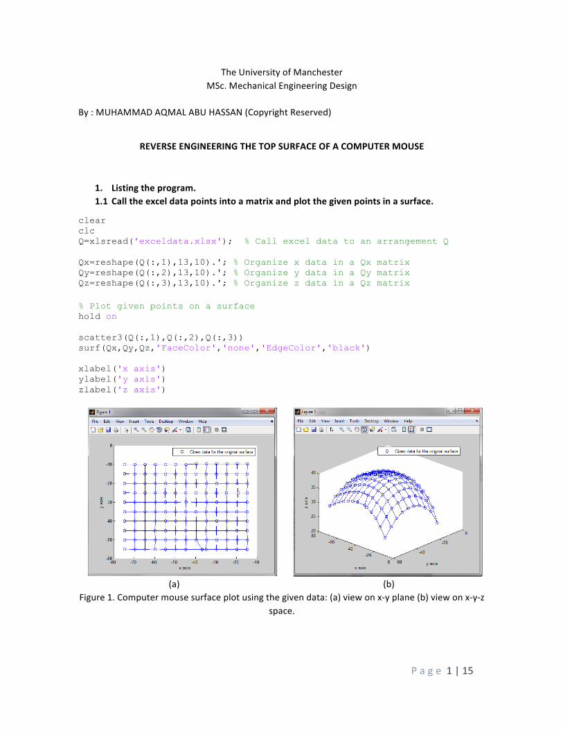
1. Listing  the  program.  1.1 Call  the  excel  data  points  into  a  matrix  and  plot  the  given  points  in  a  surface.  

clear clc Q=xlsread('exceldata.xlsx'); % Call excel data to an arrangement Q Qx=reshape(Q(:,1),13,10).'; % Organize x data in a Qx matrix Qy=reshape(Q(:,2),13,10).'; % Organize y data in a Qy matrix Qz=reshape(Q(:,3),13,10).'; % Organize z data in a Qz matrix % Plot given points on a surface hold on scatter3(Q(:,1),Q(:,2),Q(:,3)) surf(Qx,Qy,Qz,'FaceColor','none','EdgeColor','black') xlabel('x axis') ylabel('y axis') zlabel('z axis')

                     (a)                                                                                                                                                                                  (b)  

Figure  1.  Computer  mouse  surface  plot  using  the  given  data:  (a)  view  on  x-­‐y  plane  (b)  view  on  x-­‐y-­‐z  space.  

     

P a g e  2  |  15  

   

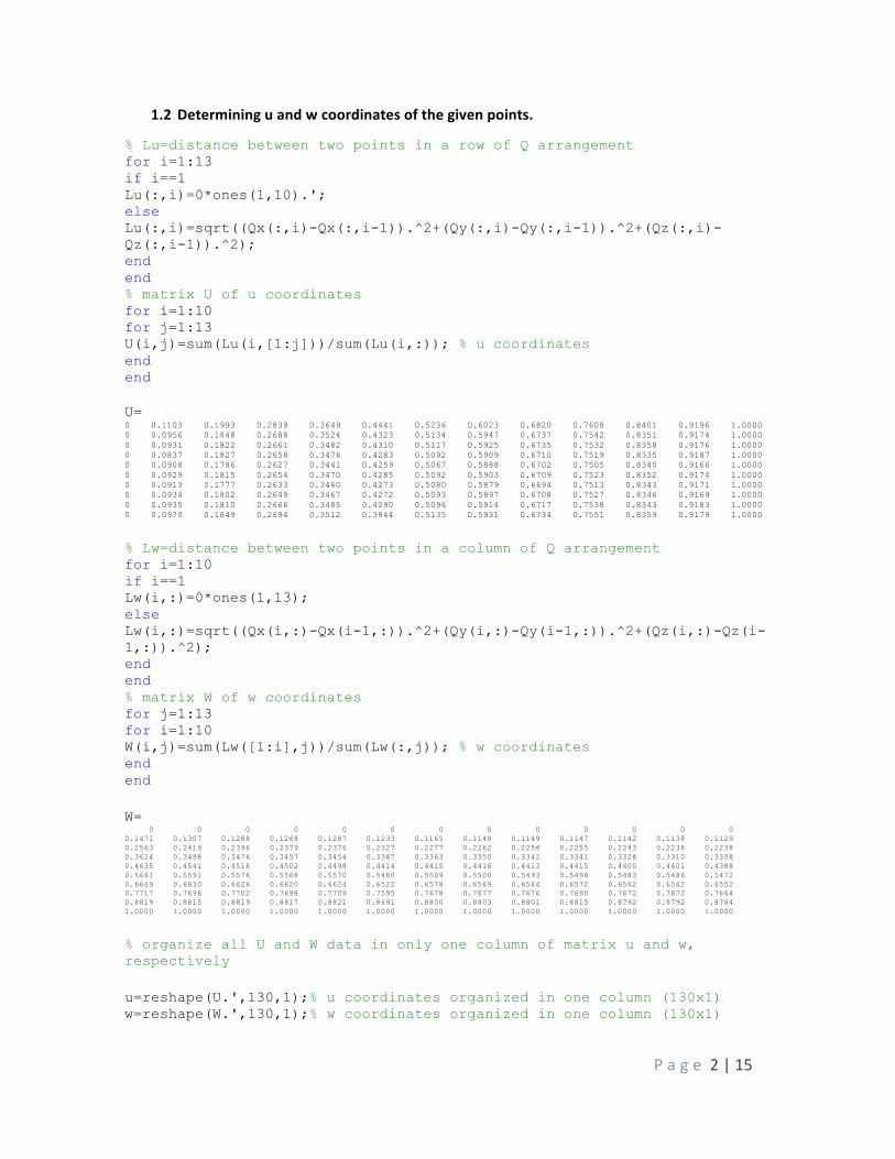
1.2 Determining  u  and  w  coordinates  of  the  given  points.  

% Lu=distance between two points in a row of Q arrangement for i=1:13 if i==1 Lu(:,i)=0*ones(1,10).'; else Lu(:,i)=sqrt((Qx(:,i)-Qx(:,i-1)).^2+(Qy(:,i)-Qy(:,i-1)).^2+(Qz(:,i)-Qz(:,i-1)).^2); end end % matrix U of u coordinates for i=1:10 for j=1:13 U(i,j)=sum(Lu(i,[1:j]))/sum(Lu(i,:)); % u coordinates end end U= 0 0.1103 0.1993 0.2839 0.3649 0.4441 0.5236 0.6023 0.6820 0.7608 0.8401 0.9196 1.0000 0 0.0956 0.1848 0.2688 0.3524 0.4323 0.5134 0.5947 0.6737 0.7542 0.8351 0.9174 1.0000 0 0.0931 0.1822 0.2661 0.3482 0.4310 0.5117 0.5925 0.6735 0.7532 0.8358 0.9176 1.0000 0 0.0837 0.1827 0.2658 0.3476 0.4283 0.5092 0.5909 0.6710 0.7519 0.8335 0.9187 1.0000 0 0.0908 0.1786 0.2627 0.3441 0.4259 0.5067 0.5888 0.6702 0.7505 0.8340 0.9166 1.0000 0 0.0929 0.1815 0.2654 0.3470 0.4285 0.5092 0.5903 0.6709 0.7523 0.8352 0.9174 1.0000 0 0.0913 0.1777 0.2633 0.3460 0.4273 0.5080 0.5879 0.6694 0.7513 0.8343 0.9171 1.0000 0 0.0934 0.1802 0.2649 0.3467 0.4272 0.5093 0.5897 0.6708 0.7527 0.8346 0.9169 1.0000 0 0.0935 0.1810 0.2666 0.3485 0.4290 0.5096 0.5914 0.6717 0.7538 0.8343 0.9183 1.0000 0 0.0970 0.1849 0.2694 0.3512 0.3844 0.5135 0.5931 0.6734 0.7551 0.8359 0.9179 1.0000

% Lw=distance between two points in a column of Q arrangement for i=1:10 if i==1 Lw(i,:)=0*ones(1,13); else Lw(i,:)=sqrt((Qx(i,:)-Qx(i-1,:)).^2+(Qy(i,:)-Qy(i-1,:)).^2+(Qz(i,:)-Qz(i-1,:)).^2); end end % matrix W of w coordinates for j=1:13 for i=1:10 W(i,j)=sum(Lw([1:i],j))/sum(Lw(:,j)); % w coordinates end end W= 0 0 0 0 0 0 0 0 0 0 0 0 0 0.1471 0.1307 0.1288 0.1268 0.1287 0.1233 0.1165 0.1148 0.1149 0.1147 0.1142 0.1138 0.1129 0.2563 0.2419 0.2396 0.2379 0.2376 0.2327 0.2277 0.2262 0.2254 0.2255 0.2243 0.2238 0.2238 0.3624 0.3498 0.3476 0.3457 0.3454 0.3387 0.3363 0.3350 0.3342 0.3341 0.3328 0.3310 0.3308 0.4635 0.4541 0.4518 0.4502 0.4498 0.4414 0.4415 0.4416 0.4413 0.4415 0.4400 0.4401 0.4388 0.5661 0.5591 0.5576 0.5568 0.5570 0.5480 0.5509 0.5500 0.5493 0.5498 0.5483 0.5486 0.5472 0.6669 0.6630 0.6626 0.6620 0.6624 0.6522 0.6578 0.6569 0.6564 0.6572 0.6562 0.6562 0.6552 0.7717 0.7696 0.7702 0.7698 0.7709 0.7595 0.7678 0.7677 0.7676 0.7690 0.7672 0.7672 0.7664 0.8819 0.8815 0.8819 0.8817 0.8821 0.8691 0.8800 0.8803 0.8801 0.8815 0.8792 0.8792 0.8784 1.0000 1.0000 1.0000 1.0000 1.0000 1.0000 1.0000 1.0000 1.0000 1.0000 1.0000 1.0000 1.0000

% organize all U and W data in only one column of matrix u and w, respectively u=reshape(U.',130,1);% u coordinates organized in one column (130x1) w=reshape(W.',130,1);% w coordinates organized in one column (130x1)

P a g e  3  |  15  

   

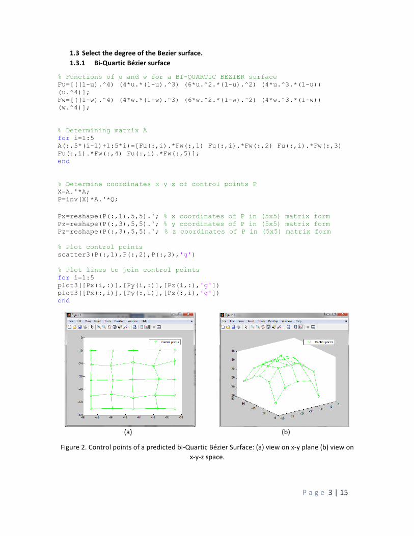
1.3 Select  the  degree  of  the  Bezier  surface.  1.3.1 Bi-­‐Quartic  Bézier  surface  

% Functions of u and w for a BI-QUARTIC BÉZIER surface Fu=[((1-u).^4) (4*u.*(1-u).^3) (6*u.^2.*(1-u).^2) (4*u.^3.*(1-u)) (u.^4)]; Fw=[((1-w).^4) (4*w.*(1-w).^3) (6*w.^2.*(1-w).^2) (4*w.^3.*(1-w)) (w.^4)];  

% Determining matrix A for i=1:5 A(:,5*(i-1)+1:5*i)=[Fu(:,i).*Fw(:,1) Fu(:,i).*Fw(:,2) Fu(:,i).*Fw(:,3) Fu(:,i).*Fw(:,4) Fu(:,i).*Fw(:,5)]; end  

% Determine coordinates x-y-z of control points P X=A.'*A; P=inv(X)*A.'*Q; Px=reshape(P(:,1),5,5).'; % x coordinates of P in (5x5) matrix form Pz=reshape(P(:,3),5,5).'; % y coordinates of P in (5x5) matrix form Pz=reshape(P(:,3),5,5).'; % z coordinates of P in (5x5) matrix form % Plot control points scatter3(P(:,1),P(:,2),P(:,3),'g') % Plot lines to join control points for i=1:5 plot3([Px(i,:)],[Py(i,:)],[Pz(i,:),'g']) plot3([Px(:,i)],[Py(:,i)],[Pz(:,i),'g']) end

(a)                                                                                                                                                                                  (b)  

Figure  2.  Control  points  of  a  predicted  bi-­‐Quartic  Bézier  Surface:  (a)  view  on  x-­‐y  plane  (b)  view  on  x-­‐y-­‐z  space.  

 

P a g e  4  |  15  

   

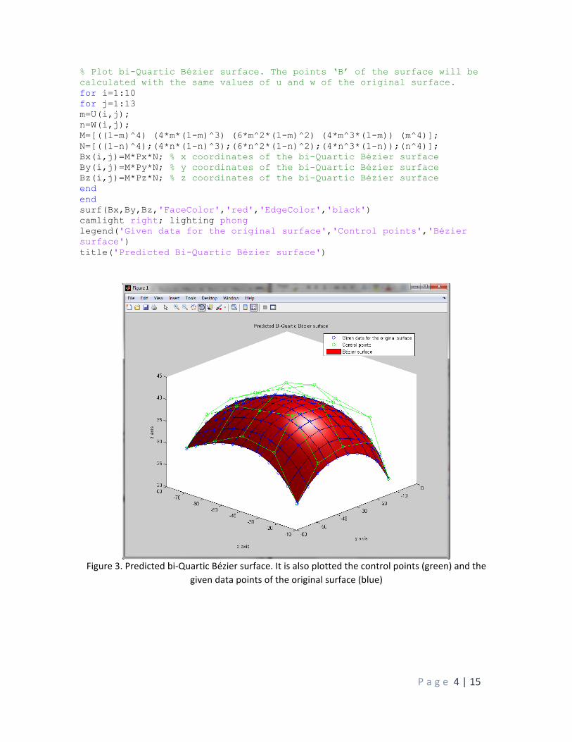
% Plot bi-Quartic Bézier surface. The points ‘B’ of the surface will be calculated with the same values of u and w of the original surface. for i=1:10 for j=1:13 m=U(i,j); n=W(i,j); M=[((1-m)^4) (4*m*(1-m)^3) (6*m^2*(1-m)^2) (4*m^3*(1-m)) (m^4)]; N=[((1-n)^4);(4*n*(1-n)^3);(6*n^2*(1-n)^2);(4*n^3*(1-n));(n^4)]; Bx(i,j)=M*Px*N; % x coordinates of the bi-Quartic Bézier surface By(i,j)=M*Py*N; % y coordinates of the bi-Quartic Bézier surface Bz(i,j)=M*Pz*N; % z coordinates of the bi-Quartic Bézier surface end end surf(Bx,By,Bz,'FaceColor','red','EdgeColor','black') camlight right; lighting phong legend('Given data for the original surface','Control points','Bézier surface') title('Predicted Bi-Quartic Bézier surface')

Figure  3.  Predicted  bi-­‐Quartic  Bézier  surface.  It  is  also  plotted  the  control  points  (green)  and  the  

given  data  points  of  the  original  surface  (blue)  

 

 

 

 

P a g e  5  |  15  

   

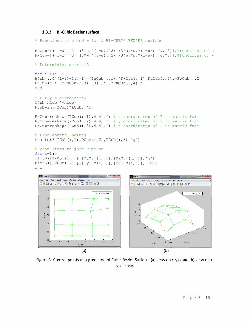
1.3.2 Bi-­‐Cubic  Bézier  surface  

% Functions of u and w for a BI-CUBIC BÉZIER surface FuCub=[((1-u).^3) (3*u.*(1-u).^2) (3*u.*u.*(1-u)) (u.^3)];%Functions of u FwCub=[((1-w).^3) (3*w.*(1-w).^2) (3*w.*w.*(1-w)) (w.^3)];%Functions of w % Determining matrix A for i=1:4 ACub(:,4*(i-1)+1:4*i)=[FuCub(:,i).*FwCub(:,1) FuCub(:,i).*FwCub(:,2) FuCub(:,i).*FwCub(:,3) Fu(:,i).*FwCub(:,4)]; end % P x-y-z coordinates XCub=ACub.'*ACub; PCub=inv(XCub)*ACub.'*Q; PxCub=reshape(PCub(:,1),4,4).'; % x coordinates of P in matrix form PyCub=reshape(PCub(:,2),4,4).'; % y coordinates of P in matrix form PzCub=reshape(PCub(:,3),4,4).'; % z coordinates of P in matrix form % Plot control points scatter3(PCub(:,1),PCub(:,2),PCub(:,3),'g') % plot lines to join P point for i=1:4 plot3([PxCub(i,:)],[PyCub(i,:)],[PzCub(i,:)],'g') plot3([PxCub(:,i)],[PyCub(:,i)],[PzCub(:,i)], 'g’) end

(a)                                                                                                                                                        (b)  

Figure  3.  Control  points  of  a  predicted  bi-­‐Cubic  Bézier  Surface:  (a)  view  on  x-­‐y  plane  (b)  view  on  x-­‐y-­‐z  space.  

P a g e  6  |  15  

   

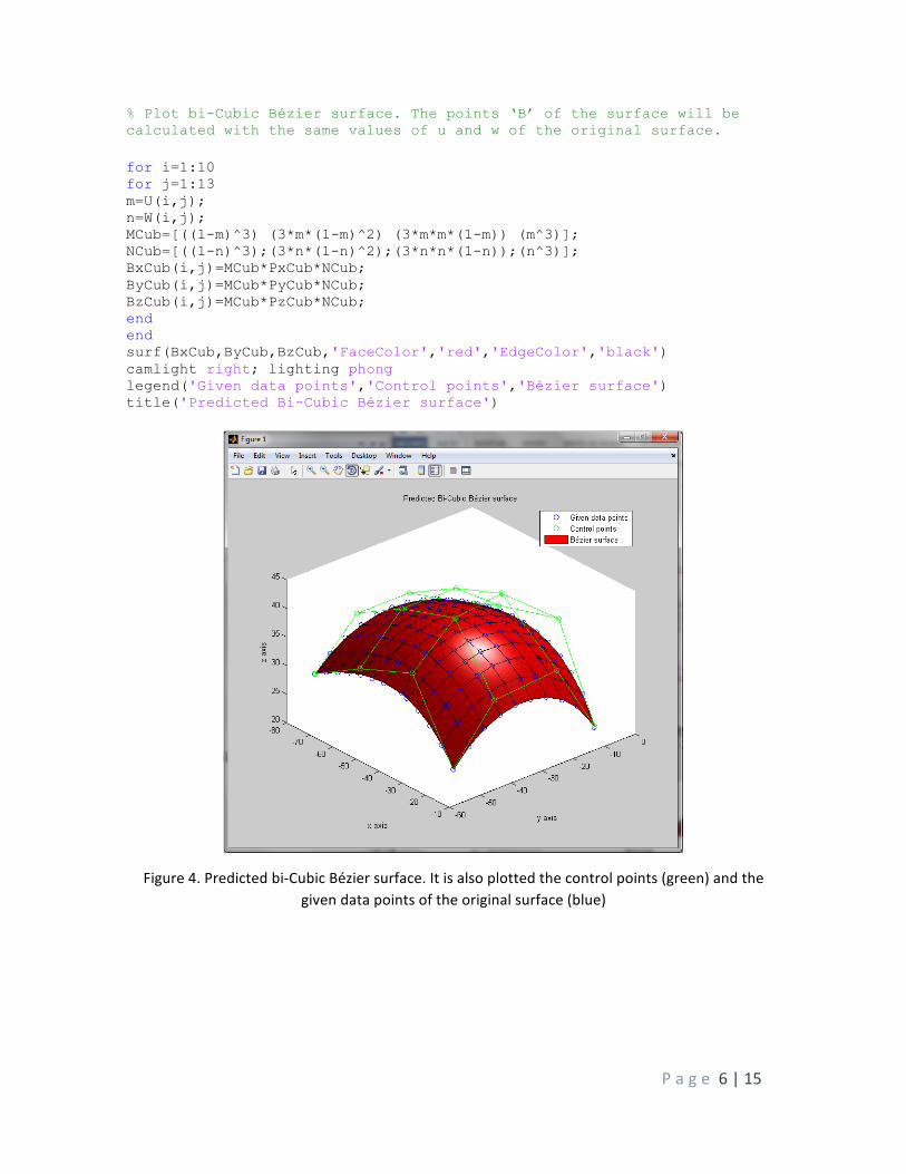
% Plot bi-Cubic Bézier surface. The points ‘B’ of the surface will be calculated with the same values of u and w of the original surface. for i=1:10 for j=1:13 m=U(i,j); n=W(i,j); MCub=[((1-m)^3) (3*m*(1-m)^2) (3*m*m*(1-m)) (m^3)]; NCub=[((1-n)^3);(3*n*(1-n)^2);(3*n*n*(1-n));(n^3)]; BxCub(i,j)=MCub*PxCub*NCub; ByCub(i,j)=MCub*PyCub*NCub; BzCub(i,j)=MCub*PzCub*NCub; end end surf(BxCub,ByCub,BzCub,'FaceColor','red','EdgeColor','black') camlight right; lighting phong legend('Given data points','Control points','Bézier surface') title('Predicted Bi-Cubic Bézier surface')

 

Figure  4.  Predicted  bi-­‐Cubic  Bézier  surface.  It  is  also  plotted  the  control  points  (green)  and  the  given  data  points  of  the  original  surface  (blue)  

 

 

 

 

P a g e  7  |  15  

   

1.3.3 Bi-­‐Quadratic  Bézier  surface    

% Functions of u and w for a BI-QUADRATIC BÉZIER surface FuQuad=[((1-u).^2) (2*u.*(1-u)) (u.^2)]; % Functions of u FwQuad=[((1-w).^2) (2*w.*(1-w)) (w.^2)]; % Functions of w % Determining matrix A for i=1:3 AQuad(:,3*(i-1)+1:3*i)=[FuQuad(:,i).*FwQuad(:,1) FuQuad(:,i).*FwQuad(:,2) FuQuad(:,i).*FwQuad(:,3)]; end % P x-y-z coordinates XQuad=AQuad.'*AQuad; PQuad=inv(XQuad)*AQuad.'*Q; PxQuad=reshape(PQuad(:,1),3,3).'; % x coordinates of P in matrix form PyQuad=reshape(PQuad(:,2),3,3).'; % y coordinates of P in matrix form PzQuad=reshape(PQuad(:,3),3,3).'; % z coordinates of P in matrix form scatter3(PQuad(:,1),PQuad(:,2),PQuad(:,3)) for i=1:3 % plot lines to join P point plot3([PxQuad(i,:)],[PyQuad(i,:)],[PzQuad(i,:)]) plot3([PxQuad(:,i)],[PyQuad(:,i)],[PzQuad(:,i)])

(a)                                                                                                                                                        (b)  

Figure  5.  Control  points  of  a  predicted  bi-­‐Quadratic  Bézier  Surface:  (a)  view  on  x-­‐y  plane  (b)  view  on  x-­‐y-­‐z  space.  

P a g e  8  |  15  

   

% Plot bi-Quadratic Bézier surface. The points ‘B’ of the surface will be calculated with the same values of u and w of the original surface. for i=1:10 for j=1:13 m=U(i,j); n=W(i,j); MQuad=[((1-m)^2) (2*m*(1-m)) (m^2)]; NQuad=[((1-n)^2);(2*n*(1-n));(n^2)]; BxQuad(i,j)=MQuad*PxQuad*NQuad; ByQuad(i,j)=MQuad*PyQuad*NQuad; BzQuad(i,j)=MQuad*PzQuad*NQuad; end end surf(BxQuad,ByQuad,BzQuad,'FaceColor','red','EdgeColor','black') camlight right; lighting phong for i=1:3 % plot lines to join P point plot3([PxQuad(i,:)],[PyQuad(i,:)],[PzQuad(i,:)]) plot3([PxQuad(:,i)],[PyQuad(:,i)],[PzQuad(:,i)]) end legend('Given data points','Control points','Bézier surface') title('Predicted Bi-Quadratic Bézier surface')  

 

Figure  6.  Predicted  bi-­‐Cubic  Bézier  surface.  It  is  also  plotted  the  control  points  (green)  and  the  given  data  points  of  the  original  surface  (blue)  

 

 

P a g e  9  |  15  

   

Original  surface  point  at  u  and  w  coordinates  

Bézier  surface  point  at  u  and  w  coordinates  

2. The  least  squares  mean  error  of  the  predicted  surface.    From  here,  a  bi-­‐Quartic  Bézier  surface  will  be  used  to  calculate  the  error  of  the  predicted  surface.        The  error  will  be  defined  as  the  distance  between  the  given  data  points  and  the  points  of  the  bi-­‐Quartic  Bézier  surface  at  each  u  and  w  coordinate.  The  mean  squared  error  will  be  then  the  sum  of  the  squares  of  all  distances  divided  to  the  number  of  points:    

𝑀𝑆𝐸 =1𝑛

(𝑑!)!!

!!!

 

Where:    MSE=  mean  squared  error  n=  number  of  points  (130)  d=distance  between  the  ith  given  data  point  at  (ui,wi)and  the  ith  point  of  the  Bézier  surface  at  (ui,wi).  

 The  error  can  be  seen  in  figure  4.    

 

Figure  7.  Zoom  to  a  random  point  of  the  surface  to  show  the  error  between  the  calculated  point  of  the  bi-­‐Quartic  Bézier  surface  and  the  given  point  in  at  the  same  u  and  w  coordinates.  

The  sub-­‐program  to  calculate  the  mean  squared  error  is  written  as  follows:   for i=1:10 for j=1:13 d(i,j)=sqrt((Bx(i,j)-Qx(i,j))^2+(By(i,j)-Qy(i,j))^2+(Bz(i,j)-Qz(i,j))^2); end end e=d.^2; MSE=sum(sum(e))/130; disp(['mean squared error is: ',num2str(MSE)]) The  mean  squared  error  calculated  is:    mean squared error is: 0.019421

P a g e  10  |  15  

 

3. Cartesian  coordinates  of  the  point  u=w=0.5  on  the  original  and  predicted  surfaces.  3.1 Cartesian  coordinates  of  the  predicted  surface.  

 Since   there   is   developed   a   function   to   calculate   the   points   of   the   predicted   bi-­‐Quartic   Bézier  surface,   it   is   only   necessary   to   define   the   variables   m   and   n,   which   represent   the   u   and   w  coordinates   of   the   predicted   surface,   to   calculate   the   points   of   the   surface.The   sub-­‐program   to  perform  this  task  is  written  as  follows:    m1=0.5; n1=0.5; M1=[((1-m1)^4) (4*m1*(1-m1)^3) (6*m1^2*(1-m1)^2) (4*m1^3*(1-m1)) (m1^4)]; N1=[((1-n1)^4);(4*n1*(1-n1)^3);(6*n1^2*(1-n1)^2);(4*n1^3*(1-n1));(n1^4)]; B1x=M1*Px*N1; B1y=M1*Py*N1; B1z=M1*Pz*N1; disp(['x coordinate of Bézier surface at u=w=0.5: ',num2str(B1x)]) disp(['y coordinate of Bézier surface at u=w=0.5: ',num2str(B1y)]) disp(['z coordinate of Bézier surface at u=w=0.5: ',num2str(B1z)])  

x  coordinate  of  Bézier  surface  at  u=w=0.5:  -­‐44.1542  y  coordinate  of  Bézier  surface  at  u=w=0.5:  -­‐32.7075  z  coordinate  of  Bézier  surface  at  u=w=0.5:  39.2047    

3.2 Cartesian  coordinates  of  the  original  surface.    There   is  no  exact  values  of  x-­‐y-­‐z  coordinates  of  the  original  surface  points  at  u=w=0.5  because   it  can  not  be   found  an  exact  value  of  u  an  w  equal   to  0.5   in   the  matrix  of   the  u  and  w  calculated  coordinates.   However,   it   can   be   interpolated   from   the   values   shown   in   table   1   and   2   which  represent  the  values  of  u  and  w  in  matrix  form,  respectively.    

Table  1.  Values  of  u  closest  to  0.5  0   0.1103   0.1993   0.2839   0.3649   0.4441   0.5236   0.6023   0.6820   0.7608   0.8401   0.9196   1  0   0.0956   0.1848   0.2688   0.3524   0.4323   0.5134   0.5947   0.6737   0.7542   0.8351   0.9174   1  0   0.0931   0.1822   0.2661   0.3482   0.4310   0.5117   0.5925   0.6735   0.7532   0.8358   0.9176   1  0   0.0837   0.1827   0.2658   0.3476   0.4283   0.5092   0.5909   0.6710   0.7519   0.8335   0.9187   1  0   0.0908   0.1786   0.2627   0.3441   0.4259   0.5067   0.5888   0.6702   0.7505   0.8340   0.9166   1  0   0.0929   0.1815   0.2654   0.3470   0.4285   0.5092   0.5903   0.6709   0.7523   0.8352   0.9174   1  0   0.0913   0.1777   0.2633   0.3460   0.4273   0.5080   0.5879   0.6694   0.7513   0.8343   0.9171   1  0   0.0934   0.1802   0.2649   0.3467   0.4272   0.5093   0.5897   0.6708   0.7527   0.8346   0.9169   1  0   0.0935   0.1810   0.2666   0.3485   0.4290   0.5096   0.5914   0.6717   0.7538   0.8343   0.9183   1  0   0.0970   0.1849   0.2694   0.3512   0.3844   0.5135   0.5931   0.6734   0.7551   0.8359   0.9179   1  

 Table  2.  Values  of  w  closest  to  0.5  

0   0   0   0   0   0   0   0   0   0   0   0   0  0.1471   0.1307   0.1288   0.1268   0.1287   0.1233   0.1165   0.1148   0.1149   0.1147   0.1142   0.1138   0.1129  0.2563   0.2419   0.2396   0.2379   0.2376   0.2327   0.2277   0.2262   0.2254   0.2255   0.2243   0.2238   0.2238  0.3624   0.3498   0.3476   0.3457   0.3454   0.3387   0.3363   0.3350   0.3342   0.3341   0.3328   0.3310   0.3308  0.4635   0.4541   0.4518   0.4502   0.4498   0.4414   0.4415   0.4416   0.4413   0.4415   0.4400   0.4401   0.4388  0.5661   0.5591   0.5576   0.5568   0.5570   0.5480   0.5509   0.5500   0.5493   0.5498   0.5483   0.5486   0.5472  0.6669   0.6630   0.6626   0.6620   0.6624   0.6522   0.6578   0.6569   0.6564   0.6572   0.6562   0.6562   0.6552  0.7717   0.7696   0.7702   0.7698   0.7709   0.7595   0.7678   0.7677   0.7676   0.7690   0.7672   0.7672   0.7664  0.8819   0.8815   0.8819   0.8817   0.8821   0.8691   0.8800   0.8803   0.8801   0.8815   0.8792   0.8792   0.8784  

1   1   1   1   1   1   1   1   1   1   1   1   1  

P a g e  11  |  15  

 

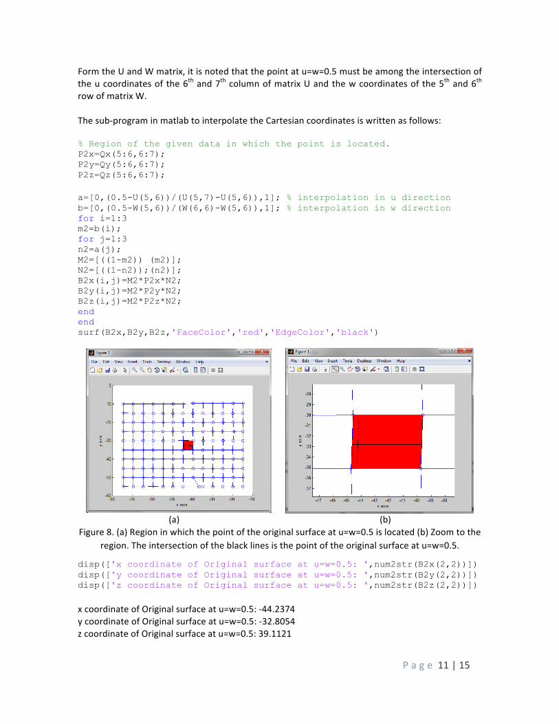
Form  the  U  and  W  matrix,  it  is  noted  that  the  point  at  u=w=0.5  must  be  among  the  intersection  of  the  u  coordinates  of  the  6th  and  7th  column  of  matrix  U  and  the  w  coordinates  of  the  5th  and  6th  row  of  matrix  W.    The  sub-­‐program  in  matlab  to  interpolate  the  Cartesian  coordinates  is  written  as  follows:    % Region of the given data in which the point is located.  P2x=Qx(5:6,6:7); P2y=Qy(5:6,6:7); P2z=Qz(5:6,6:7); a=[0,(0.5-U(5,6))/(U(5,7)-U(5,6)),1]; % interpolation in u direction b=[0,(0.5-W(5,6))/(W(6,6)-W(5,6)),1]; % interpolation in w direction for i=1:3 m2=b(i); for j=1:3 n2=a(j); M2=[((1-m2)) (m2)]; N2=[((1-n2));(n2)]; B2x(i,j)=M2*P2x*N2; B2y(i,j)=M2*P2y*N2; B2z(i,j)=M2*P2z*N2; end end surf(B2x,B2y,B2z,'FaceColor','red','EdgeColor','black')

             (a)                                                                                                                                                                                (b)  

Figure  8.  (a)  Region  in  which  the  point  of  the  original  surface  at  u=w=0.5  is  located  (b)  Zoom  to  the  region.  The  intersection  of  the  black  lines  is  the  point  of  the  original  surface  at  u=w=0.5.  

disp(['x coordinate of Original surface at u=w=0.5: ',num2str(B2x(2,2))]) disp(['y coordinate of Original surface at u=w=0.5: ',num2str(B2y(2,2))]) disp(['z coordinate of Original surface at u=w=0.5: ',num2str(B2z(2,2))])  x  coordinate  of  Original  surface  at  u=w=0.5:  -­‐44.2374  y  coordinate  of  Original  surface  at  u=w=0.5:  -­‐32.8054  z  coordinate  of  Original  surface  at  u=w=0.5:  39.1121    

P a g e  12  |  15  

 

Table  3.  Cartesian  coordinates  of  the  points  of  the  Bézier  surface  and  Original  surface  at  u=w=0.5  

  Bézier  Surface   Original  Surface  x  coordinate  at  u=w=0.5   -­‐44.1542   -­‐44.2374  y  coordinate  at  u=w=0.5   -­‐32.7075   -­‐32.8054  z  coordinate  at  u=w=0.5   39.2047   39.1121  

 4. Alternate  shapes  of  the  top  surface  of  the  mouse.  

 Several  alternate  surfaces  are  suggested  by  changing  the  values  of  the  coordinates  of  the  control  points  of  the  bi-­‐Qurtic  Bézier  surface.  This  suggested  values  are  shown  in  table  4:    Table  4.  Cartesian  coordinates  in  matrix  form  of  the  bi-­‐Quartic  Bézier  surface  control  points  for  the  

suggested  alternate  surfaces  S1,  S2  and  S3.  

  Surface  S1   Surface  S2   Surface  S3  

x  coordinates  

-­‐20   -­‐15   -­‐12   -­‐15   -­‐20   -­‐15   -­‐10   -­‐8   -­‐10   -­‐15   -­‐15   -­‐6   -­‐5   -­‐8   -­‐17  -­‐30   -­‐30   -­‐30   -­‐30   -­‐30   -­‐30   -­‐30   -­‐30   -­‐30   -­‐30   -­‐30   -­‐25   -­‐26   -­‐28   -­‐30  

-­‐45   -­‐45   -­‐45   -­‐45   -­‐45   -­‐45   -­‐45   -­‐45   -­‐45   -­‐45   -­‐45   -­‐45   -­‐45   -­‐45   -­‐45  -­‐60   -­‐60   -­‐60   -­‐60   -­‐60   -­‐60   -­‐60   -­‐60   -­‐60   -­‐60   -­‐63   -­‐64   -­‐64   -­‐65   -­‐65  

-­‐70   -­‐75   -­‐77   -­‐75   -­‐70   -­‐75   -­‐80   -­‐83   -­‐80   -­‐75   -­‐77   -­‐82   -­‐84   -­‐82   -­‐76  

y  coordinates  

-­‐15   -­‐20   -­‐30   -­‐40   -­‐45   -­‐12   -­‐20   -­‐30   -­‐40   -­‐48   -­‐15   -­‐20   -­‐30   -­‐40   -­‐50  -­‐10   -­‐20   -­‐30   -­‐40   -­‐50   -­‐12   -­‐21   -­‐30   -­‐39   -­‐48   -­‐13   -­‐23   -­‐32   -­‐42   -­‐52  

-­‐10   -­‐20   -­‐30   -­‐40   -­‐50   -­‐15   -­‐25   -­‐30   -­‐35   -­‐45   -­‐15   -­‐25   -­‐34   -­‐43   -­‐53  -­‐10   -­‐20   -­‐30   -­‐40   -­‐50   -­‐15   -­‐25   -­‐30   -­‐35   -­‐45   -­‐17   -­‐26   -­‐35   -­‐44   -­‐53  

-­‐15   -­‐20   -­‐30   -­‐40   -­‐45   -­‐18   -­‐25   -­‐30   -­‐35   -­‐42   -­‐19   -­‐26   -­‐33   -­‐42   -­‐51  

z  coordinates  

22   32   33   32   22   22   32   33   32   24   22   32   33   32   24  28   40   41   40   28   34   40   41   40   34   34   40   41   40   34  

30   41   43   41   30   35   41   43   40   35   35   41   43   40   35  

28   38   40   38   28   35   38   40   38   32   35   38   40   38   32  22   34   36   34   22   31   35   36   34   28   31   35   36   34   28  

 The  sub-­‐program  to  calculate  the  corresponding  bi-­‐Quartic  Bézier  surface  is  written  as  follows:                            

P a g e  13  |  15  

 

% ALTERNATE SUGGESTED SURFACE 1 % Suggested control points for alternate surfaces S1Px=[[-20 -15 -12 -15 -20];[-30 -30 -30 -30 -30];[-45 -45 -45 -45 -45];[-60 -60 -60 -60 -60 ];[-70 -75 -77 -75 -70]]; S1Py=[[-15 -20 -30 -40 -45];[-10 -20 -30 -40 -50];[-10 -20 -30 -40 -50];[-10 -20 -30 -40 -50];[-15 -20 -30 -40 -45]]; S1Pz=[[22 32 33 32 22];[28 40 41 40 28];[30 41 43 41 30];[28 38 40 38 28];[22 34 36 34 22]]; % Calculate points of suggested bi-Quartic Bézier surface for i=1:10 for j=1:13 m=U(i,j); n=W(i,j); M=[((1-m)^4) (4*m*(1-m)^3) (6*m^2*(1-m)^2) (4*m^3*(1-m)) (m^4)]; N=[((1-n)^4);(4*n*(1-n)^3);(6*n^2*(1-n)^2);(4*n^3*(1-n));(n^4)]; S1Bx(i,j)=M*S1Px*N; S1By(i,j)=M*S1Py*N; S1Bz(i,j)=M*S1Pz*N; end end figure hold on % Plot control points for i=1:5 scatter3(S1Px(:,i),S1Py(:,i),S1Pz(:,i),'g') plot3([S1Px(i,:)],[S1Py(i,:)],[S1Pz(i,:)],'g') plot3([S1Px(:,i)],[S1Py(: ,i)],[S1Pz(:,i)],'g') end % Plot the suggested surface S1 surf(S1Bx,S1By,S1Bz,'FaceColor','blue','EdgeColor','black') camlight right; lighting phong legend('Control points for the suggested bi-Quartic Bézier Surface 1') title('Suggested bi-Quartic Bézier surface 1') xlabel('x axis') ylabel('y axis') zlabel('z axis')

             (a)                                                                                                                                                                                  (b)  

Figure  9.  Alternate  shape  bi-­‐Quartic  Bézier  surface  S1:  (a)  view  on  x-­‐y  plane  (b)  view  on  x-­‐y-­‐z  space.  

P a g e  14  |  15  

 

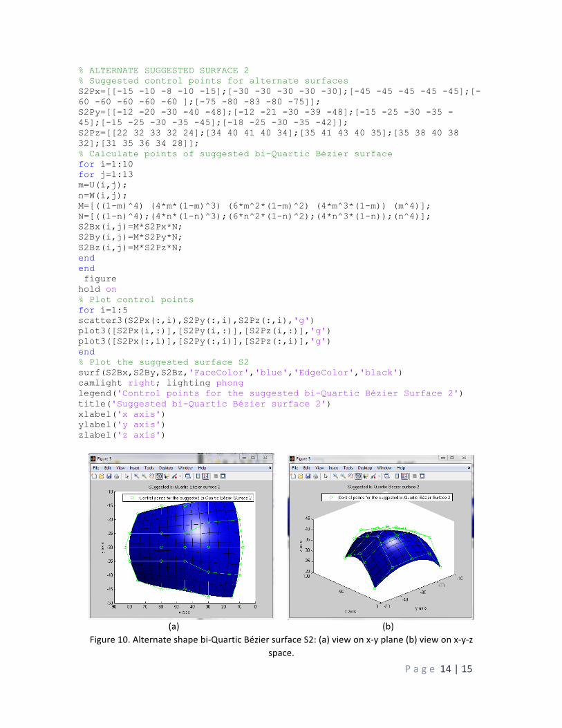
% ALTERNATE SUGGESTED SURFACE 2 % Suggested control points for alternate surfaces S2Px=[[-15 -10 -8 -10 -15];[-30 -30 -30 -30 -30];[-45 -45 -45 -45 -45];[-60 -60 -60 -60 -60 ];[-75 -80 -83 -80 -75]]; S2Py=[[-12 -20 -30 -40 -48];[-12 -21 -30 -39 -48];[-15 -25 -30 -35 -45];[-15 -25 -30 -35 -45];[-18 -25 -30 -35 -42]]; S2Pz=[[22 32 33 32 24];[34 40 41 40 34];[35 41 43 40 35];[35 38 40 38 32];[31 35 36 34 28]]; % Calculate points of suggested bi-Quartic Bézier surface for i=1:10 for j=1:13 m=U(i,j); n=W(i,j); M=[((1-m)^4) (4*m*(1-m)^3) (6*m^2*(1-m)^2) (4*m^3*(1-m)) (m^4)]; N=[((1-n)^4);(4*n*(1-n)^3);(6*n^2*(1-n)^2);(4*n^3*(1-n));(n^4)]; S2Bx(i,j)=M*S2Px*N; S2By(i,j)=M*S2Py*N; S2Bz(i,j)=M*S2Pz*N; end end figure hold on % Plot control points for i=1:5 scatter3(S2Px(:,i),S2Py(:,i),S2Pz(:,i),'g') plot3([S2Px(i,:)],[S2Py(i,:)],[S2Pz(i,:)],'g') plot3([S2Px(:,i)],[S2Py(:,i)],[S2Pz(:,i)],'g') end % Plot the suggested surface S2 surf(S2Bx,S2By,S2Bz,'FaceColor','blue','EdgeColor','black') camlight right; lighting phong legend('Control points for the suggested bi-Quartic Bézier Surface 2') title('Suggested bi-Quartic Bézier surface 2') xlabel('x axis') ylabel('y axis') zlabel('z axis')  

             (a)                                                                                                                                                                                  (b)  

Figure  10.  Alternate  shape  bi-­‐Quartic  Bézier  surface  S2:  (a)  view  on  x-­‐y  plane  (b)  view  on  x-­‐y-­‐z  space.  

P a g e  15  |  15  

 

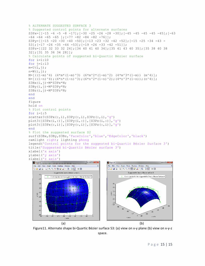
% ALTERNATE SUGGESTED SURFACE 3 % Suggested control points for alternate surfaces S3Px=[[-15 -6 -5 -8 -17];[-30 -25 -26 -28 -30];[-45 -45 -45 -45 -45];[-63 -64 -64 -65 -65 ];[-77 -82 -84 -82 -76]]; S3Py=[[-15 -20 -30 -40 -50];[-13 -23 -32 -42 -52];[-15 -25 -34 -43 -53];[-17 -26 -35 -44 -53];[-19 -26 -33 -42 -51]]; S3Pz=[[22 32 33 32 24];[34 40 41 40 34];[35 41 43 40 35];[35 38 40 38 32];[31 35 36 34 28]]; % Calculate points of suggested bi-Quartic Bézier surface for i=1:10 for j=1:13 m=U(i,j); n=W(i,j); M=[((1-m)^4) (4*m*(1-m)^3) (6*m^2*(1-m)^2) (4*m^3*(1-m)) (m^4)]; N=[((1-n)^4);(4*n*(1-n)^3);(6*n^2*(1-n)^2);(4*n^3*(1-n));(n^4)]; S3Bx(i,j)=M*S3Px*N; S3By(i,j)=M*S3Py*N; S3Bz(i,j)=M*S3Pz*N; end end figure hold on % Plot control points for i=1:5 scatter3(S3Px(:,i),S3Py(:,i),S3Pz(:,i),'g') plot3([S3Px(i,:)],[S3Py(i,:)],[S3Pz(i,:)],'g') plot3([S3Px(:,i)],[S3Py(:,i)],[S3Pz(:,i)],'g') end % Plot the suggested surface S2 surf(S3Bx,S3By,S3Bz,'FaceColor','blue','EdgeColor','black') camlight right; lighting phong legend('Control points for the suggested bi-Quartic Bézier Surface 3') title('Suggested bi-Quartic Bézier surface 3') xlabel('x axis') ylabel('y axis') zlabel('z axis')

                 (a)                                                                                                                                                                                  (b)  

Figure11.  Alternate  shape  bi-­‐Quartic  Bézier  surface  S3:  (a)  view  on  x-­‐y  plane  (b)  view  on  x-­‐y-­‐z  space.