Computer-aided diagnosis of Alzheimer's disease using support vector machines and

classification trees

This content has been downloaded from IOPscience. Please scroll down to see the full text.

Download details:

IP Address: 61.160.126.157

This content was downloaded on 03/10/2013 at 07:16

Please note that terms and conditions apply.

2010 Phys. Med. Biol. 55 2807

(http://iopscience.iop.org/0031-9155/55/10/002)

View the table of contents for this issue, or go to the journal homepage for more

Home Search Collections Journals About Contact us My IOPscience

IOP PUBLISHING PHYSICS IN MEDICINE AND BIOLOGY

Phys. Med. Biol. 55 (2010) 2807–2817 doi:10.1088/0031-9155/55/10/002

Computer-aided diagnosis of Alzheimer’s diseaseusing support vector machines and classification trees

D Salas-Gonzalez1, J M Gorriz1, J Ramırez1, M Lopez1, I Alvarez1,F Segovia1, R Chaves1 and C G Puntonet2

1 Department of Signal Theory Networking and Communications, ETSIIT, 18071, University ofGranada, Spain2 Department of Computer Architecture and Computer Technology, ETSIIT, 18071, University ofGranada, Spain

E-mail: dsalas@ugr.es

Received 29 September 2009, in final form 25 March 2010Published 22 April 2010Online at stacks.iop.org/PMB/55/2807

AbstractThis paper presents a computer-aided diagnosis technique for improving theaccuracy of early diagnosis of Alzheimer-type dementia. The proposedmethodology is based on the selection of voxels which present Welch’st-test between both classes, normal and Alzheimer images, greater than a giventhreshold. The mean and standard deviation of intensity values are calculatedfor selected voxels. They are chosen as feature vectors for two differentclassifiers: support vector machines with linear kernel and classificationtrees. The proposed methodology reaches greater than 95% accuracy in theclassification task.

(Some figures in this article are in colour only in the electronic version)

1. Introduction

Distinguishing Alzheimer’s disease (AD) remains a diagnostic challenge, especially duringthe early stage of the disease. Furthermore, in this early stage, the disease offers betteropportunities to be treated. With the growth of the older population in developed nations,the prevalence of AD is expected to quadruple over the next 50 years (Evans et al 1989,Brookmeyer et al 1998, 2007).

Single photon emission computed tomography (SPECT) is a widely used techniqueto study the functional properties of the brain. SPECT brain imaging techniques employradioisotopes which decay, emitting predominantly a single gamma photon. When the nucleusof a radioisotope disintegrates, a gamma photon is emitted in a random direction which isuniformly distributed in the sphere surrounding the nucleus. If the photon is unimpeded by acollision with electrons or other particles within the body, its trajectory will be a straight lineor ray. In order for a photon detector external to the patient to discriminate the direction that

0031-9155/10/102807+11$30.00 © 2010 Institute of Physics and Engineering in Medicine Printed in the UK 2807

2808 D Salas-Gonzalez et al

a ray is incident from, a physical collimation is required. Typically, lead collimator plates areplaced prior to the the detector’s crystal in such a manner that the photons incident from allbut a single direction are blocked by the plates. This guarantees that only photons incidentfrom the desired direction will strike the photon detector. SPECT has become an importantdiagnostic and research tool in nuclear medicine.

In SPECT images, the differences between different brains make the normalization ofthe images with respect to a reference template necessary. The general affine model, with 12parameters, is usually chosen as a first step in a normalization algorithm before proceedingwith a more complex non-rigid spatial transformation model (Salas-Gonzalez et al 2008,Friston et al 2007).

Alzheimer’s diagnosis is usually based on the information provided by a careful clinicalexamination, a thorough interview of the patient and relatives and a neuropsychologicalassessment (Braak and Braak 1997, Cummings et al 1998, Hoffman et al 2000, Ng et al2007). A SPECT study is frequently used as a complimentary diagnostic tool in addition tothe clinical findings (Silverman et al 2001, Higdon et al 2004). However, in late-onset ADthere is minimal perfusion in the mild stages of the disease, and age-related changes, whichare frequently seen in healthy aged people, have to be discriminated from minimal disease-specific changes. These minimal changes in the images make visual diagnosis a difficult taskthat requires experienced experts.

This paper presents a computer-aided diagnosis system for the early detection ofAlzheimer-type dementia (ATD) using support vector machines (SVM) and classificationtrees (CT). SVM is a powerful tool which has recently been the focus of attention for theclassification of tomography brain images (Ramırez et al 2010, Gorriz et al 2008, Fung andStoeckel 2007). In this work, we compare the performance of both classifiers, SVM and CT,using the accuracy rate, sensitivity and specificity.

In the proposed methodology, Welch’s t-test is performed in each voxel of the brain imagefor mean normal and mean Alzheimer’s disease images. The set of voxels which presentgreater values than different thresholds are selected. The mean and standard deviation of theseselected voxels are used as features of the classifiers.

This work is organized as follows: in section 2 we present an overview of the supportvector machines and the classification trees; in section 3, the SPECT image acquisition andimage preprocessing steps are explained; we discuss the construction of the feature vector insection 4; in section 5, we summarize the classification performance obtained for linear supportvector machine and classification trees and, finally, conclusions are drawn in section 6.

2. Overview of the classifiers

The images we work with belong to two different classes: normal controls and Alzheimer-type dementia (ATD). The goal of the classification task is to separate a set of binary labeledtraining data consisting of, in the general case, N-dimensional patterns vi and class labels yi:

(v1, y1), (v2, y2), . . . , (vl , yl) ∈ (RN × {−1, +1}), (1)

so that a classifier is produced which maps an object vi to its classification label yi where yi iseither 1 or −1, indicating the class to which the point vi belongs. This classifier will have theability to classify new test samples.

2.1. Support vector machines with linear kernels

Linear discriminant functions define decision hypersurfaces or hyperplanes in amultidimensional feature space:

Diagnosing Alzheimer’s using SVM and CT 2809

g(v) = wT v + w0 = 0 (2)

where w is the weight vector and w0 is the threshold. w is orthogonal to the decisionhyperplane. The goal is to find the unknown parameters wi, i = 1, . . . , N , which define thedecision hyperplane (Vapnik 1998).

Let vi , i = 1, 2, . . . , l, be the feature vectors of the training set. These belong to twodifferent classes, ω1 or ω2. If the classes are linearly separable, the objective is to designa hyperplane that classifies correctly all the training vectors. This hyperplane is not uniqueand it can be estimated maximizing the performance of the classifier, that is, the ability of theclassifier to operate satisfactorily with new data. The maximal margin of separation betweenboth classes is a useful design criterion. Since the distance from a point v to the hyperplaneis given by z = |g(v)|/‖w‖, the optimization problem can be reduced to the maximization ofthe margin 2/‖w‖ with constraints by scaling w and w0 so that the value of g(v) is +1 for thenearest point in w1 and −1 for the nearest point in w2. The constraints are as follows:

wT v + w0 � 1, ∀ v ∈ w1 (3)

wT v + w0 � 1, ∀ v ∈ w2, (4)

or, equivalently, minimizing the cost function J (w) = 1/2‖w‖2 subject to

yi(wT vi + w0) � 1, i = 1, 2, . . . , l. (5)

Let us relate the mathematical symbols in this section with the actual variables used inthis work (see sections 4 and 5 for a more detailed explanation of these variables). In the casein which the mean and standard deviation of selected voxels are chosen as features, vector v isa two-dimensional (N = 2) vector. Therefore, for a given image i the vector of the features isvi = (μi, σi), where μi is the mean of intensity values for selected voxels (those voxels withWelch’s t-test value greater than a given threshold value ε) in image i. Furthermore, σi is thestandard deviation of selected voxels. Lastly, l denotes the number of images (l = 79).

2.2. Classification trees

Classification trees is a non-parametric technique that produces classification of categoricaldependent variables (Breiman et al 1993). Binary tree-structured classifiers are constructedby repeated splits of subsets of X into two descendant subsets, beginning with X itself, where Xdenotes the measurement space to be defined as containing all possible measurement vectors.For instance, in this work in the case in which two features are chosen, X is a two-dimensionalspace such that the first coordinate (mean of selected voxels) ranges over all real valuesbetween [0–255]. The second coordinate, standard deviation of selected voxels, is defined ascontinuously ranging from [0, +∞] although in practice, in our work it takes values from 10to 70 (see the axis range in figures 6 and 7).

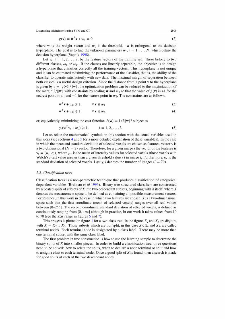
This process is plotted in figure 1 for a two-class tree. In the figure, X2 and X3 are disjointwith X = X2 ∪ X3. Those subsets which are not split, in this case X2, X4 and X5, are calledterminal nodes. Each terminal node is designated by a class label. There may be more thanone terminal subset with the same class label.

The first problem in tree construction is how to use the learning sample to determine thebinary splits of X into smaller pieces. In order to build a classification tree, three questionsneed to be solved: how to select the splits, when to declare a node terminal or split and howto assign a class to each terminal node. Once a good split of X is found, then a search is madefor good splits of each of the two descendant nodes.

2810 D Salas-Gonzalez et al

Figure 1. Hypothetical two-class tree.

Classification and regression trees (CART) was developed by Leo Breiman (Breimanet al 1993). We refer to this book to get a deep insight into CART techniques and theirmathematical foundations. The first problem in tree construction is how to use the learningsample to determine the binary splits of X into smaller and smaller pieces. The fundamentalidea is to select each split of a subset so that the data in each of the descendant subsets are‘purer’ than the data in the parent subset. Therefore, a mathematical measure of ‘impurity’needs to be addressed such that the node impurity is largest when all classes are equally mixedtogether in it, and smallest when the node contains only one class.

Analogous to the last subsection, for the sake of clarity, let us relate the mathematicalsymbols and terminology in this section with the actual variables used in this work, for instance,figure 7 where the pairwise relationship between the mean and standard deviation of selectedvoxels for threshold ε = 7 is plotted. This figure suggests a possible classification rule whichcould be obtained automatically using CART to explain the first split in figure 1: (i) X isthe feature mean of selected voxels. (ii) split 1 is the following condition for each image i,μi < 150. Let us note that figure 7 shows that all the samples which fulfill this condition areATD images (denoted as red crosses). Therefore, in this example, after the training procedure,a given test image will be classified as ATD if the mean of selected voxels (with ε = 7)is μi < 150. Therefore, ‘class 1’ under the X2 box would be ATD. On the other hand, ifμi > 150, the CART algorithm automatically calculates other classification rule, which is notreported here, denoted as split 2 in figure 1.

3. SPECT image acquisition and preprocessing

The patients were injected with a gamma emitting 99mTc-ECD radiopharmaceutical and theSPECT raw data were acquired by a three head gamma camera Picker Prism 3000. Atotal of 180 projections were taken for each patient with a 2◦ angular resolution. Theimages of the brain cross sections were reconstructed from the projection data using thefiltered backprojection (FBP) algorithm in combination with a Butterworth noise removalfilter (Vandenberghea et al 2001, Bruyant 2002, Zhou and Luo 2006, Ramırez et al 2008).

The complexity of brain structures and the differences between brains of different subjectsmake the normalization of the images with respect to a common template necessary. Thisensures that the voxels in different images refer to the same anatomical positions in the brain.

Diagnosing Alzheimer’s using SVM and CT 2811

Mean Normal Image

0

50

100

150

200

250

(a)

Mean ATD Image

0

50

100

150

200

250

(b)

Figure 2. (a) Normal mean SPECT brain image INOR. (b) Alzheimer-type dementia mean SPECTbrain image IATD.

In this work, the images have been normalized using a general affine model, with 12 parameters(Hill et al 2001, Salas-Gonzalez et al 2008, Woods et al 1998).

After the affine normalization, the resulting image is registered using a more complexnon-rigid spatial transformation model. The deformations are parameterized by a linearcombination of the lowest frequency components of the three-dimensional cosine transformbases (Ashburner and Friston 1999). A small-deformation approach is used, and regularizationis by the bending energy of the displacement field. Then, we normalize the intensities of theSPECT images with respect to the maximum intensity, which is computed for each imageindividually by averaging over 3% of the highest voxel intensities, similarly as in Saxena et al(1998).

4. Feature selection: Welch’s t-test

We study the main differences between normal and Alzheimer-type dementia images. Voxelswhich provide a higher difference between both groups will be considered as training vectorsof two classifiers: support vector machines with linear kernel and classification trees. Thus,this statistical study will allow us to select discriminant regions of the brain to establish whethera given SPECT image belongs to a normal or an ATD patient.

Figure 2(a) shows the mean SPECT brain image of normal subjects INOR and 2(b) themean ATD image IATD. They are very similar; nevertheless, there are some regions of themean normal brain which present higher intensity values.

The root-mean-square deviation of the images from their mean for normal controls andATD images are defined as INOR

σ and IATDσ . They are plotted in figures 3(a) and (b). These

figures help us to discriminate those areas of the brain which present lower dispersion betweenimages.

Welch’s t-test for independent samples is a modification of the t-test that does not assumeequal population variances. Using the information provided by the mean and standarddeviation normal and ATD images, the t-test can be calculated for each voxel by

I t = INOR − IATD√I σ

NORNNOR

+ I σATD

NATD

, (6)

2812 D Salas-Gonzalez et al

Std Normal Image

0

10

20

30

(a)

Std ATD Image

0

10

20

30

(b)

Figure 3. (a) Standard deviation image of normal subjects IσNOR. (b) Standard deviation image of

ATD subjects IσATD.

−4 −2 0 2 4 6 8 10 120

500

1000

1500

2000

2500

3000

3500

4000

4500

# o

f vo

xe

ls

It(i)

(a)

t−test Image

−2

0

2

4

6

8

10

(b)

Figure 4. (a) Histogram representing the distribution of the t-values for the image I t (i).(b) Welch’s t-test image It.

where It denotes the resulting image with the value given by Welch’s t-test calculated in eachvoxel. Figure 4 depicts this image It. The histogram with the distribution of It is plotted infigure 4(b).

Welch’s t-test gives us a value which allows us to measure the voxel intensity differencebetween the mean normal (INOR) and mean ATD image (IATD). Those voxels which present at-test value greater than a given threshold will be selected for the classification task.

5. Results

The performance of the classification is tested on a set of 79 real SPECT images (41 normal and38 ATD) using the leave one-out method: the classifier is trained with all but one image of thedatabase. The remaining image, which is not used to define the classifier, is then categorized.In that way, all SPECT images are classified and the success rate is computed from the number

Diagnosing Alzheimer’s using SVM and CT 2813

−2 0 2 4 6 80.6

0.65

0.7

0.75

0.8

0.85

0.9

0.95

1

Threshold, ε

Accu

racy

SVM Linear

Class. Trees

(a)

−2 0 2 4 6 80.6

0.65

0.7

0.75

0.8

0.85

0.9

0.95

1

Threshold, ε

Accu

racy

SVM Linear

Class. Trees

(b)

Figure 5. Accuracy rate versus threshold value ε. Feature vector: (a) mean of selected voxels.(b) Mean and standard deviation of selected voxels.

of correctly classified subjects. This process is repeated such that each observation in thesample is used once as the validation data.

First of all, we select those voxels i which fulfill the following condition:

i / {I t (i) > ε}, (7)

where ε is a threshold. We choose 25 threshold values equally spaced from −3 to 9. Thenumber of selected voxels decreases as ε increases. Increasing ε allows us to select thosevoxels which present a greater difference between the mean normal and ATD images accordingto Welch’s t-test. Two different features will be used: on the one hand, mean of selected voxelsand, on the other hand, a vector with two components: mean and standard deviation of selectedvoxels.

The classification performance obtained using support vector machines with linear kerneland classification trees versus the threshold value ε is plotted in figure 5. As expected, theclassification accuracy is lower for small threshold values ε and increases concomitantly withε. Using both set of features, it is easily seen that support vector machines present, in general,a higher correct rate than classification trees except for very high values of ε. On the otherhand, better results are obtained using mean and standard deviation as features. For instance,this fact is remarked in the case in which ε > 4. The best accuracy rate (96.2%) was obtainedwhen the threshold was set to ε > 8 and classification was performed using classification trees.Other classifiers such as support vector machines with quadratic kernel, radial basis functionand Fisher-linear discriminant analysis have also been used for classification purposes. Theypresent very similar performance to the SVM with linear kernels used in this work. Theseresults have not been included in the figure for the sake of clarity.

As expected, higher accuracy rates are obtained for higher values of ε. This is due tothe fact that feature vectors separate better both classes (normal and ATD) as the thresholdvalue increases. This fact is shown by means of scatter plots: in order to show the pairwiserelationship between the mean and standard deviation of selected voxels for two differentvalues of the threshold (ε = 0 and ε = 7) two matrix plots are drawn (figures 6 and 7,respectively). These figures show that, as it was pointed out before, the selected features aremore separated for normal and ADT images when ε = 7 than in the case ε = 0.

2814 D Salas-Gonzalez et al

50 55 60 65 70

Std

90 100 110

50

55

60

65

7085

90

95

100

105

110

Mean

Normal

ATD

ε = 0

Figure 6. Matrix plot ε = 0.

15 20 25

Std

120 140 160 180

15

20

25

120

140

160

180

Mean

Normal

ATD

ε = 7

Figure 7. Matrix plot ε = 7.

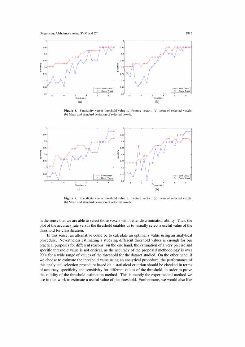
The accuracy rate does not give us a complete overview of the performance of theclassification, hence sensitivity and specificity have been calculated. The sensitivity measuresthe proportion of actual positives which are correctly identified while the specificity measuresgive us the proportion of negatives which are correctly identified. Figures 8 and 9 plot thesensitivity versus threshold values. In general, we obtain higher sensitivity using support vectormachines than using decision trees. Nevertheless, decision trees achieve higher specificitythan SVM for high threshold values.

In this work, we also choose ε = 0 or even voxels with Welch’s t-test with ε < 0, onlyto estimate the performance of the classification task for different threshold values and tohighlight the improvement of the accuracy of the proposed methodology concomitantly withthe value of ε. This procedure allows us to easily estimate an ‘optimal’ value of the threshold

Diagnosing Alzheimer’s using SVM and CT 2815

−2 0 2 4 6 80.6

0.65

0.7

0.75

0.8

0.85

0.9

0.95

1

Threshold, ε

Se

nsitiv

ity

SVM Linear

Class. Trees

(a)

−2 0 2 4 6 80.6

0.65

0.7

0.75

0.8

0.85

0.9

0.95

1

Threshold, ε

Se

nsitiv

ity

SVM Linear

Class. Trees

(b)

Figure 8. Sensitivity versus threshold value ε. Feature vector: (a) mean of selected voxels.(b) Mean and standard deviation of selected voxels.

−2 0 2 4 6 80.6

0.65

0.7

0.75

0.8

0.85

0.9

0.95

1

Threshold, ε

Sp

ecific

ity

SVM Linear

Class. Trees

(a)

−2 0 2 4 6 80.6

0.65

0.7

0.75

0.8

0.85

0.9

0.95

1

Threshold, ε

Sp

ecific

ity

SVM Linear

Class. Trees

(b)

Figure 9. Specificity versus threshold value ε. Feature vector: (a) mean of selected voxels.(b) Mean and standard deviation of selected voxels.

in the sense that we are able to select those voxels with better discrimination ability. Thus, theplot of the accuracy rate versus the threshold enables us to visually select a useful value of thethreshold for classification.

In this sense, an alternative could be to calculate an optimal ε value using an analyticalprocedure. Nevertheless estimating ε studying different threshold values is enough for ourpractical purposes for different reasons: on the one hand, the estimation of a very precise andspecific threshold value is not critical, as the accuracy of the proposed methodology is over90% for a wide range of values of the threshold for the dataset studied. On the other hand, ifwe choose to estimate the threshold value using an analytical procedure, the performance ofthis analytical selection procedure based on a statistical criterion should be checked in termsof accuracy, specificity and sensitivity for different values of the threshold, in order to provethe validity of the threshold estimation method. This is merely the experimental method weuse in that work to estimate a useful value of the threshold. Furthermore, we would also like

2816 D Salas-Gonzalez et al

to point out that the estimation of a useful value of ε, similarly to the training procedure, onlyneeds to be performed once as a ‘batch’ process.

6. Conclusion

In this work, a computer-aided diagnosis technique for the diagnosis of Alzheimer-typedementia (ATD) is presented. Initially, the images were labeled by experts as normal orAlzheimer’s dementia. After normalization of the brain images, we calculate the mean normaland mean ATD image. Welch’s t-test between both images is calculated in each voxel. Theresulting statistic t gives us a procedure to ranking voxels. Voxels with t-values greater thandifferent threshold values are selected. The mean and standard deviation of selected voxelsare used as feature vectors for two different classifiers: a support vector machine with linearkernel and a classification tree. The accuracy, sensitivity and specificity of both classifiersare analyzed using several threshold values. The proposed methodology reaches up to 96.2%accuracy in the classification task. The method proposed in this work allows us to classify thebrain images in normal and affected subjects in a parsimonious way, with no prior knowledgeabout Alzheimer’s disease.

Acknowledgments

This work was partly supported by the MICINN of Spain under the PETRI DENCLASES(PET2006-0253), TEC2008-02113, NAPOLEON (TEC2007-68030-C02-01) and HD2008-0029 projects and the Consejerıa de Innovacion, Ciencia y Empresa (Junta de Andalucıa,Spain) under the Excellence Projects TIC-02566 and TIC-4530. We also thank the reviewersfor their careful reading of the manuscript and helpful comments.

References

Ashburner J and Friston K J 1999 Nonlinear spatial normalization using basis functions Hum. Brain Mapp. 7 254–66Braak H and Braak E 1997 Diagnostic criteria for neuropathologic assessment of Alzheimer’s disease Neurobiol.

Aging 18 S85–8Breiman L, Friedman J H, Olshen R A and Stone C J 1993 Classification and Regression Trees (London: Chapman

& Hall)Brookmeyer R, Gray S and Kawas C 1998 Projections of Alzheimer’s disease in the United States and the public

health impact of delaying disease onset J. Am. Med. Assoc. 88 1337–42Brookmeyer R, Johnson E, Ziegler-Graham K and Arrighi M 2007 Forecasting the global burden of Alzheimer’s

disease Alzheimer’s Dementia 3 186–91Bruyant P P 2002 Analytic and iterative reconstruction algorithms in SPECT J. Nucl. Med. 43 1343–58Cummings J L, Vinters H V, Cole G M and Khachaturian Z S 1998 Alzheimer’s disease: etiologies, pathophysiology,

cognitive reserve, and treatment opportunities Neurology 51 (Suppl. 1) S2–17Evans D, Funkenstein H, Albert M, Scherr P, Cook N, Chown M, Hebert L, Hennekens C and Taylor J 1989 Prevalence

of Alzheimer’s disease in a community population of older persons: higher than previously reported J. Am.Med. Assoc. 262 2551–6

Friston K, Ashburner J, Kiebel S, Nichols T and Penny W (ed) 2007 Statistical Parametric Mapping: The Analysisof Functional Brain Images (New York: Academic)

Fung G and Stoeckel J 2007 SVM feature selection for classification of SPECT images of Alzheimer’s disease usingspatial information Knowl. Inf. Syst. 11 243–58

Gorriz J M, Ramırez J, Lassl A, Salas-Gonzalez D, Lang E W, Puntonet C G, Alvarez I, Lopez M and Gomez-Rıo M2008 Automatic computer aided diagnosis tool using component-based SVM Medical Imaging Conf., Dresden(Piscataway, NJ: IEEE)

Higdon R et al 2004 A comparison of classification methods for differentiating fronto-temporal dementia fromAlzheimer’s disease using FDG-PET imaging Stat. Med. 23 315–26

Diagnosing Alzheimer’s using SVM and CT 2817

Hill D L G, Batchelor P G, Holden M and Hawkes D J 2001 Medical image registration Phys. Med. Biol. 46 R1–45Hoffman J M, Welsh-Bohmer K A and Hanson M 2000 FDG PET Imaging in patients with pathologically verified

dementia J. Nucl. Med. 41 1920–8Ng S et al 2007 Visual assessment versus quantitative assessment of 11C-PIB PET and 18F-FDG PET for detection

of Alzheimer’s disease J. Nucl. Med. 48 547–52Ramırez J, Gorriz J M, Gomez-Rıo M, Romero A, Chaves R, Lassl A, Rodrıguez A, Puntonet C G, Theis F and

Lang E 2008 Effective emission tomography image reconstruction algorithms for SPECT data ICCS 2008,Part I (LNCS vol 5101/2008) (Berlin: Springer) pp 741–8

Ramırez J, Gorriz J M, Romero A, Lassl A, Salas-Gonzalez D, Lopez M, Gomez-Rıo M and Rodrıguez A 2010Computer aided diagnosis of Alzheimer type dementia combining support vector machines and discriminant setof features Inf. Sci. at press (http://dx.doi.org/10.1016/j.ins.2009.05.012)

Salas-Gonzalez D, Gorriz J M, Ramırez J, Lassl A and Puntonet C G 2008 Improved Gauss–Newton optimizationmethods in affine registration of SPECT brain images IET Electron. Lett. 44 1291–2

Saxena P, Pavel D G, Quintana J C and Horwitz B 1998 An automatic threshold-based scaling method forenhancing the usefulness of Tc-HMPAO SPECT in the diagnosis of Alzheimer’s disease Medical ImageComputing and Computer-Assisted Intervention—MICCAI (Lecture Notes in Computer Science vol 1496)(Berlin: Springer) pp 623–30

Silverman D H, Small G W and Chang C Y 2001 Positron emission tomography in evaluation of dementia: regionalbrain metabolism and long-term outcome J. Am. Med. Assoc. 286 2120–7

Vandenberghea S, D’Asselera Y, de Wallea R V, Kauppinenb T, Koolea M, Bouwensa L, Laerec K V, Lemahieua Iand Dierckx R 2001 Iterative reconstruction algorithms in nuclear medicine Comput. Med. ImagingGraph. 25 105–11

Vapnik V 1998 Statistical Learning Theory (New York: Wiley)Woods R P, Grafton S T, Holmes C J, Cherry S R and Mazziotta J C 1998 Automated image registration: I. General

methods and intrasubject, intramodality validation J. Comput. Assist. Tomogr. 22 139–52Zhou J and Luo L M 2006 Sequential weighted least squares algorithm for PET image reconstruction Digit. Signal

Process. 16 735–45