Computer-Aided Colorectal Tumor Classification in NBI Endoscopy Using Local Features

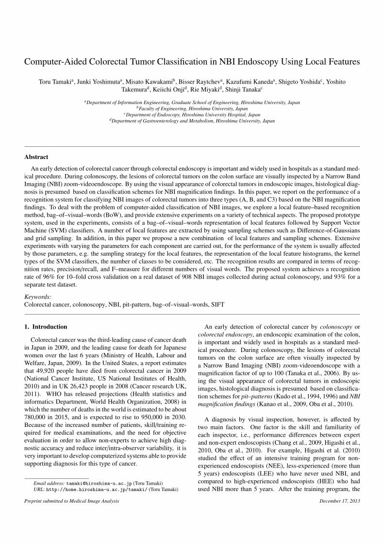
Computer-Aided Colorectal Tumor Classification in NBI Endoscopy Using Local Features

Toru Tamakia, Junki Yoshimutaa, Misato Kawakamib, Bisser Raytcheva, Kazufumi Kanedaa, Shigeto Yoshidac, YoshitoTakemurad, Keiichi Onjid, Rie Miyakid, Shinji Tanakac

aDepartment of Information Engineering, Graduate School of Engineering, Hiroshima University, JapanbFaculty of Engineering, Hiroshima University, Japan

cDepartment of Endoscopy, Hiroshima University Hospital, JapandDepartment of Gastroenterology and Metabolism, Hiroshima University, Japan

Abstract

An early detection of colorectal cancer through colorectal endoscopy is important and widely used in hospitals as a standard med-ical procedure. During colonoscopy, the lesions of colorectal tumors on the colon surface are visually inspected by a Narrow BandImaging (NBI) zoom-videoendoscope. By using the visual appearance of colorectal tumors in endoscopic images, histological diag-nosis is presumed based on classification schemes for NBI magnification findings. In this paper, we report on the performance of arecognition system for classifying NBI images of colorectal tumors into three types (A, B, and C3) based on the NBI magnificationfindings. To deal with the problem of computer-aided classification of NBI images, we explore a local feature–based recognitionmethod, bag–of–visual–words (BoW), and provide extensive experiments on a variety of technical aspects. The proposed prototypesystem, used in the experiments, consists of a bag–of–visual–words representation of local features followed by Support VectorMachine (SVM) classifiers. A number of local features are extracted by using sampling schemes such as Difference-of-Gaussiansand grid sampling. In addition, in this paper we propose a new combination of local features and sampling schemes. Extensiveexperiments with varying the parameters for each component are carried out, for the performance of the system is usually affectedby those parameters, e.g. the sampling strategy for the local features, the representation of the local feature histograms, the kerneltypes of the SVM classifiers, the number of classes to be considered, etc. The recognition results are compared in terms of recog-nition rates, precision/recall, and F–measure for different numbers of visual words. The proposed system achieves a recognitionrate of 96% for 10–fold cross validation on a real dataset of 908 NBI images collected during actual colonoscopy, and 93% for aseparate test dataset.

Keywords:Colorectal cancer, colonoscopy, NBI, pit-pattern, bag–of–visual–words, SIFT

1. Introduction

Colorectal cancer was the third-leading cause of cancer deathin Japan in 2009, and the leading cause for death for Japanesewomen over the last 6 years (Ministry of Health, Labour andWelfare, Japan, 2009). In the United States, a report estimatesthat 49,920 people have died from colorectal cancer in 2009(National Cancer Institute, US National Institutes of Health,2010) and in UK 26,423 people in 2008 (Cancer research UK,2011). WHO has released projections (Health statistics andinformatics Department, World Health Organization, 2008) inwhich the number of deaths in the world is estimated to be about780,000 in 2015, and is expected to rise to 950,000 in 2030.Because of the increased number of patients, skill/training re-quired for medical examinations, and the need for objectiveevaluation in order to allow non-experts to achieve high diag-nostic accuracy and reduce inter/intra-observer variability, it isvery important to develop computerized systems able to providesupporting diagnosis for this type of cancer.

Email address: [email protected] (Toru Tamaki)URL: http://home.hiroshima-u.ac.jp/tamaki/ (Toru Tamaki)

An early detection of colorectal cancer by colonoscopy orcolorectal endoscopy, an endoscopic examination of the colon,is important and widely used in hospitals as a standard med-ical procedure. During colonoscopy, the lesions of colorectaltumors on the colon surface are often visually inspected bya Narrow Band Imaging (NBI) zoom-videoendoscope with amagnification factor of up to 100 (Tanaka et al., 2006). By us-ing the visual appearance of colorectal tumors in endoscopicimages, histological diagnosis is presumed based on classifica-tion schemes for pit–patterns (Kudo et al., 1994, 1996) and NBImagnification findings (Kanao et al., 2009, Oba et al., 2010).

A diagnosis by visual inspection, however, is affected bytwo main factors. One factor is the skill and familiarity ofeach inspector, i.e., performance differences between expertand non-expert endoscopists (Chang et al., 2009, Higashi et al.,2010, Oba et al., 2010). For example, Higashi et al. (2010)studied the effect of an intensive training program for non-experienced endoscopists (NEE), less-experienced (more than5 years) endoscopists (LEE) who have never used NBI, andcompared to high-experienced endoscopists (HEE) who hadused NBI more than 5 years. After the training program, the

Preprint submitted to Medical Image Analysis December 17, 2013

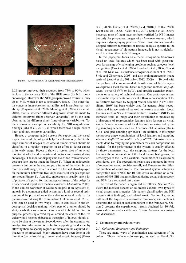
Figure 1: A screen shot of an actual NBI zoom-videoendoscopiy.

LLE group improved their accuracy from 73% to 90%, whichis close to the accuracy 93% of the HEE group (for NBI zoom-endoscopy). However, the NEE group improved from 63% onlyup to 74%, which is not a satisfactory result. The other fac-tor concerns inter-observer variability and intra-observer vari-ability (Mayinger et al., 2006, Meining et al., 2004, Oba et al.,2010), that is, whether different diagnoses would be made bydifferent observers (inter-observer variability), or by the sameobserver at the different times (intra-observer variability). Ta-ble 2 shows an example of variability for NBI magnificationfindings (Oba et al., 2010), in which there was a high level ofinter- and intra-observer variability.

Hence, a computer-aided system for supporting the visualinspection would be of great help for colonoscopy, due to thelarge number of images of colorectal tumors which should beclassified in a regular inspection in an effort to detect cancerin its early stage. Figure 1 shows a screen shot of an actualmonitor at which endoscopists and doctors are looking duringendoscopy. The monitor displays the live video from a videoen-doscope (the largest image in Figure 1). When an endoscopistpresses a button on the endoscope, a frame of the video is cap-tured as a still image, which is stored to a file and also displayedon the monitor below the live video (four still images capturedare shown Figure 1). Actually, endoscopists usually take a lotof pictures of a polyp for finding a good image of the polyp fora paper-based report with medical evidences (Aabakken, 2009).In the clinical workflow, it would be helpful if an objective di-agnosis by a computer-aided system as a kind of second opin-ion could be provided onto the video monitor directly or forpictures taken during the examination (Takemura et al., 2012).This can be used in two ways. First, it can assist in the en-doscopist’s decision-making which part of a tumor should beshot, or whether some more pictures need to be taken. For thispurpose, processing a fixed region around the center of the livevideo would be enough because the region of interest should al-ways be shot at the center. Second, even after the examination,an objective information is useful for supporting the doctors byallowing them to specify regions of interest in the captured stillimages to be processed. Many attempts have been done in thisdirection (i.e., classifying trimmed endoscopic images) (Gross

et al., 2009b, Hafner et al., 2009a,b,c,d, 2010a,b, 2009e, 2008,Kwitt and Uhl, 2008, Kwitt et al., 2010, Stehle et al., 2009),however, most of them have not been verified for NBI imagesbut only for pit–pattern images of a chromoendoscopy, whichrequires a dye-spraying process. Since those studies have de-veloped different techniques of texture analysis specific to thevisual appearance of pit–pattern images, it is not straightfor-ward to extend them to NBI images.

In this paper, we focus on a recent recognition frameworkbased on local features which has been used with great suc-cess for a range of challenging problems such as category-levelrecognition (Csurka et al., 2004, Lazebnik et al., 2006, Nowaket al., 2006) as well as instance recognition (Chum et al., 2007,Sivic and Zisserman, 2003) and also endomicroscopic imageretrieval (Andre et al., 2011a,b,c, 2012, 2009). To deal withthe problem of computer-aided classification of NBI images,we explore a local feature–based recognition method, bag–of–visual–words (BoVW or BoW), and provide extensive experi-ments on a variety of technical aspects. Our prototype systemused in the experiments consists of a BoW representation of lo-cal features followed by Support Vector Machine (SVM) clas-sifiers. BoW has been widely used for general object recog-nition and image retrieval as well as texture analysis. Localfeatures such as Scale Invariant Feature Transform (SIFT) areextracted from an image and their distribution is modeled bya histogram of representative features (also known as visualwords, VWs). A number of local features are extracted by us-ing sampling schemes such as Difference-of-Gaussians (DoG–SIFT) and grid sampling (gridSIFT). In addition, in this paperwe propose a new combination of local features and samplingschemes, DiffSIFT and multi-scale gridSIFT. Extensive experi-ments done by varying the parameters for each component areneeded, for the performance of the system is usually affectedby those parameters, e.g. the sampling strategy for the localfeatures, the representation of the local feature histograms, thekernel types of the SVM classifiers, the number of classes to beconsidered, etc. The recognition results are compared in termsof recognition rates, precision/recall, and F–measure for differ-ent numbers of visual words. The proposed system achieves arecognition rate of 96% for 10–fold cross validation on a realdataset of 908 NBI images collected during actual colonoscopy,and 93% for a separated test dataset.

The rest of the paper is organized as follows: Section 2 re-views the medical aspects of colorectal cancers, two types ofvisual assessment strategies (pit–pattern classification and NBImagnification findings), and related work. Section 3 gives anoutline of the bag–of–visual–words framework, and Section 4describes the details of each component of the framework. Sec-tion 5 presents the experimental results obtained for 10–foldcross validation and a test dataset. Section 6 shows conclusionsand discussions.

2. Colonoscopy and related work

2.1. Colorectal Endoscopy and PathologyThere are many ways of examination and screening of the

colon. Those include colonoscopy, as well as Fecal Oc-

2

cult Blood Test (FOBT) (Heitman et al., 2008, Sanford andMcPherson, 2009), Digital Rectal Examination (DRE) (Gopal-swamy et al., 2000), biomedical markers (Karl et al., 2008),CT colonography (Halligan and Taylor, 2007, Yoshida andDachman, 2004), MR colonography (Beets and Beets-Tan,2010, Shin et al., 2010), Marvin Positron Emission Tomogra-phy (PET) (Lin et al., 2011), Ultrasound (Padhani, 1999), Dou-ble Contrast Barium Enema (DCBE) (Canon, 2008, Johnsonet al., 2004), Confocal Laser Endomicroscopy (CLE) (Kiesslichet al., 2007), and Virtual Endoscopy (Oto, 2002). Inter-ested readers are referred to the following surveys on colorec-tal cancer screening and clinical staging of colorectal cancer(Barabouti and Wong, 2005, Jenkinson and Steele, 2010, Twee-dle et al., 2007) and endoscopic imaging devices (Gaddam andSharma, 2010).

The “gold standard” (Hafner et al., 2010a) for colon ex-amination is colonoscopy, an endoscopy for the colon, whichhas been commonly used since the middle of the last century(Classen et al., 2010). Colonoscopy is an examination with avideo-endoscope equipped with a CCD camera of size less than1.4 cm in diameter at the top of the scope, as well as a lightsource and a tube for dye spraying and surgical devices for En-doscopic Mucosal Resection (EMR) (Ye et al., 2008). 1

Colorectal polyps detected during colonoscopy are histologi-cally identified as cancers (carcinomas) or non-cancers throughbiopsy, by removing the lesions from the colon surface. Thepolyps are histologically classified into the following groups(Hirata et al., 2007a,b, Kanao et al., 2009, Raghavendra et al.,2010): hyperplasias (HP), tubular adenomas (TA), carcino-mas with intramucosal invasion to scanty submucosal invasion(M/SM-s) and carcinomas with massive submucosal invasion(SM-m). TA, M/SM-s and SM-m are also referred to as neo-plastic, and HP and normal tissue as non-neoplastic.

HP are non-neoplastic and hence not removed. TA are polypsand likely to develop into cancer (many cancers follow thisadenoma-carcinoma sequence (Gloor, 1986)) and can be endo-scopically resected (i.e., removed during colonoscopy). M/SM-s cancers can also be endoscopically resected, while SM-mcancers should be surgically resected (Watanabe et al., 2012).Since SM-m cancers deeply invade the colonal surface, it isdifficult to remove them completely by colonoscopy due to thehigher risk of lymph node metastasis.

SM-m cancers need to be discriminated from M/SM-s can-cers and TA polyps without biopsy because the risk of compli-cations during colonoscopy should be minimized by avoidingunnecessary biopsy. Biopsy also tends to be avoided becausethe biopsied tumor develops to a fibrosis (Matsumoto et al.,2010) which causes a perforation at the time of surgery. Whilethere is controversy about the benefit of avoiding biopsy (Ger-shman and Ament, 2012), recent advances in the field of med-ical devices (Gaddam and Sharma, 2010) would allow the en-doscopic assessment of histology to be established and docu-mented without biopsy in the near future (Rex et al., 2011).

1Also such devices are used for Endoscopic Piecemeal Mucosal Resection(EPMR) (Tamegai, 2007), or Endoscopic Submucosal Dissection (ESD) (Saitoet al., 2007).

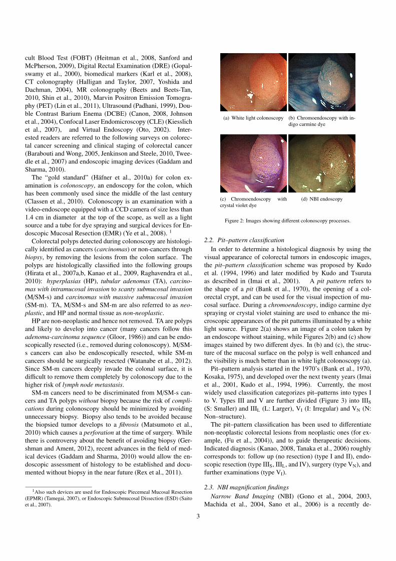
(a) White light colonoscopy (b) Chromoendoscopy with in-digo carmine dye

(c) Chromoendoscopy withcrystal violet dye

(d) NBI endoscopy

Figure 2: Images showing different colonoscopy processes.

2.2. Pit–pattern classificationIn order to determine a histological diagnosis by using the

visual appearance of colorectal tumors in endoscopic images,the pit–pattern classification scheme was proposed by Kudoet al. (1994, 1996) and later modified by Kudo and Tsurutaas described in (Imai et al., 2001). A pit pattern refers tothe shape of a pit (Bank et al., 1970), the opening of a col-orectal crypt, and can be used for the visual inspection of mu-cosal surface. During a chromoendoscopy, indigo carmine dyespraying or crystal violet staining are used to enhance the mi-croscopic appearances of the pit patterns illuminated by a whitelight source. Figure 2(a) shows an image of a colon taken byan endoscope without staining, while Figures 2(b) and (c) showimages stained by two different dyes. In (b) and (c), the struc-ture of the mucosal surface on the polyp is well enhanced andthe visibility is much better than in white light colonoscopy (a).

Pit–pattern analysis started in the 1970’s (Bank et al., 1970,Kosaka, 1975), and developed over the next twenty years (Imaiet al., 2001, Kudo et al., 1994, 1996). Currently, the mostwidely used classification categorizes pit–patterns into types Ito V. Types III and V are further divided (Figure 3) into IIIS(S: Smaller) and IIIL (L: Larger), VI (I: Irregular) and VN (N:Non–structure).

The pit–pattern classification has been used to differentiatenon-neoplastic colorectal lesions from neoplastic ones (for ex-ample, (Fu et al., 2004)), and to guide therapeutic decisions.Indicated diagnosis (Kanao, 2008, Tanaka et al., 2006) roughlycorresponds to: follow up (no resection) (type I and II), endo-scopic resection (type IIIS, IIIL, and IV), surgery (type VN), andfurther examinations (type VI).

2.3. NBI magnification findingsNarrow Band Imaging (NBI) (Gono et al., 2004, 2003,

Machida et al., 2004, Sano et al., 2006) is a recently de-

3

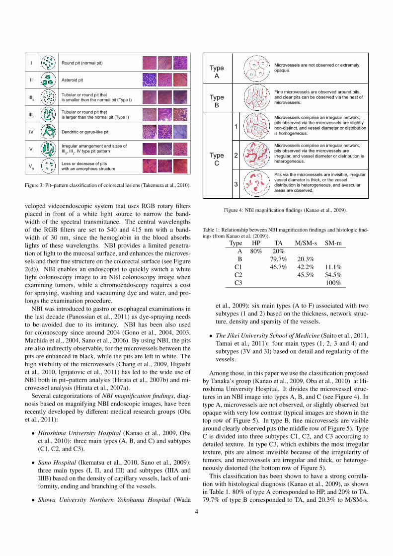
Figure 3: Pit–pattern classification of colorectal lesions (Takemura et al., 2010).

veloped videoendoscopic system that uses RGB rotary filtersplaced in front of a white light source to narrow the band-width of the spectral transmittance. The central wavelengthsof the RGB filters are set to 540 and 415 nm with a band-width of 30 nm, since the hemoglobin in the blood absorbslights of these wavelengths. NBI provides a limited penetra-tion of light to the mucosal surface, and enhances the microves-sels and their fine structure on the colorectal surface (see Figure2(d)). NBI enables an endoscopist to quickly switch a whitelight colonoscopy image to an NBI colonoscopy image whenexamining tumors, while a chromoendoscopy requires a costfor spraying, washing and vacuuming dye and water, and pro-longs the examination procedure.

NBI was introduced to gastro or esophageal examinations inthe last decade (Panossian et al., 2011) as dye-spraying needsto be avoided due to its irritancy. NBI has been also usedfor colonoscopy since around 2004 (Gono et al., 2004, 2003,Machida et al., 2004, Sano et al., 2006). By using NBI, the pitsare also indirectly observable, for the microvessels between thepits are enhanced in black, while the pits are left in white. Thehigh visibility of the microvessels (Chang et al., 2009, Higashiet al., 2010, Ignjatovic et al., 2011) has led to the wide use ofNBI both in pit–pattern analysis (Hirata et al., 2007b) and mi-crovessel analysis (Hirata et al., 2007a).

Several categorizations of NBI magnification findings, diag-nosis based on magnifying NBI endoscopic images, have beenrecently developed by different medical research groups (Obaet al., 2011):

• Hiroshima University Hospital (Kanao et al., 2009, Obaet al., 2010): three main types (A, B, and C) and subtypes(C1, C2, and C3).

• Sano Hospital (Ikematsu et al., 2010, Sano et al., 2009):three main types (I, II, and III) and subtypes (IIIA andIIIB) based on the density of capillary vessels, lack of uni-formity, ending and branching of the vessels.

• Showa University Northern Yokohama Hospital (Wada

Figure 4: NBI magnification findings (Kanao et al., 2009).

Table 1: Relationship between NBI magnification findings and histologic find-ings (from Kanao et al. (2009)).

Type HP TA M/SM-s SM-mA 80% 20%B 79.7% 20.3%

C1 46.7% 42.2% 11.1%C2 45.5% 54.5%C3 100%

et al., 2009): six main types (A to F) associated with twosubtypes (1 and 2) based on the thickness, network struc-ture, density and sparsity of the vessels.

• The Jikei University School of Medicine (Saito et al., 2011,Tamai et al., 2011): four main types (1, 2, 3 and 4) andsubtypes (3V and 3I) based on detail and regularity of thevessels.

Among those, in this paper we use the classification proposedby Tanaka’s group (Kanao et al., 2009, Oba et al., 2010) at Hi-roshima University Hospital. It divides the microvessel struc-tures in an NBI image into types A, B, and C (see Figure 4). Intype A, microvessels are not observed, or slightly observed butopaque with very low contrast (typical images are shown in thetop row of Figure 5). In type B, fine microvessels are visiblearound clearly observed pits (the middle row of Figure 5). TypeC is divided into three subtypes C1, C2, and C3 according todetailed texture. In type C3, which exhibits the most irregulartexture, pits are almost invisible because of the irregularity oftumors, and microvessels are irregular and thick, or heteroge-neously distorted (the bottom row of Figure 5).

This classification has been shown to have a strong correla-tion with histological diagnosis (Kanao et al., 2009), as shownin Table 1. 80% of type A corresponded to HP, and 20% to TA.79.7% of type B corresponded to TA, and 20.3% to M/SM-s.

4

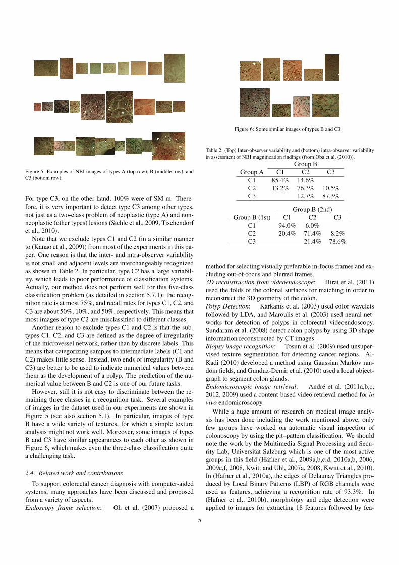
Figure 5: Examples of NBI images of types A (top row), B (middle row), andC3 (bottom row).

For type C3, on the other hand, 100% were of SM-m. There-fore, it is very important to detect type C3 among other types,not just as a two-class problem of neoplastic (type A) and non-neoplastic (other types) lesions (Stehle et al., 2009, Tischendorfet al., 2010).

Note that we exclude types C1 and C2 (in a similar mannerto (Kanao et al., 2009)) from most of the experiments in this pa-per. One reason is that the inter- and intra-observer variabilityis not small and adjacent levels are interchangeably recognizedas shown in Table 2. In particular, type C2 has a large variabil-ity, which leads to poor performance of classification systems.Actually, our method does not perform well for this five-classclassification problem (as detailed in section 5.7.1): the recog-nition rate is at most 75%, and recall rates for types C1, C2, andC3 are about 50%, 10%, and 50%, respectively. This means thatmost images of type C2 are misclassified to different classes.

Another reason to exclude types C1 and C2 is that the sub-types C1, C2, and C3 are defined as the degree of irregularityof the microvessel network, rather than by discrete labels. Thismeans that categorizing samples to intermediate labels (C1 andC2) makes little sense. Instead, two ends of irregularity (B andC3) are better to be used to indicate numerical values betweenthem as the development of a polyp. The prediction of the nu-merical value between B and C2 is one of our future tasks.

However, still it is not easy to discriminate between the re-maining three classes in a recognition task. Several examplesof images in the dataset used in our experiments are shown inFigure 5 (see also section 5.1). In particular, images of typeB have a wide variety of textures, for which a simple textureanalysis might not work well. Moreover, some images of typesB and C3 have similar appearances to each other as shown inFigure 6, which makes even the three-class classification quitea challenging task.

2.4. Related work and contributions

To support colorectal cancer diagnosis with computer-aidedsystems, many approaches have been discussed and proposedfrom a variety of aspects;Endoscopy frame selection: Oh et al. (2007) proposed a

Figure 6: Some similar images of types B and C3.

Table 2: (Top) Inter-observer variability and (bottom) intra-observer variabilityin assessment of NBI magnification findings (from Oba et al. (2010)).

Group BGroup A C1 C2 C3

C1 85.4% 14.6%C2 13.2% 76.3% 10.5%C3 12.7% 87.3%

Group B (2nd)Group B (1st) C1 C2 C3

C1 94.0% 6.0%C2 20.4% 71.4% 8.2%C3 21.4% 78.6%

method for selecting visually preferable in-focus frames and ex-cluding out-of-focus and blurred frames.3D reconstruction from videoendoscope: Hirai et al. (2011)used the folds of the colonal surfaces for matching in order toreconstruct the 3D geometry of the colon.Polyp Detection: Karkanis et al. (2003) used color waveletsfollowed by LDA, and Maroulis et al. (2003) used neural net-works for detection of polyps in colorectal videoendoscopy.Sundaram et al. (2008) detect colon polyps by using 3D shapeinformation reconstructed by CT images.Biopsy image recognition: Tosun et al. (2009) used unsuper-vised texture segmentation for detecting cancer regions. Al-Kadi (2010) developed a method using Gaussian Markov ran-dom fields, and Gunduz-Demir et al. (2010) used a local object-graph to segment colon glands.Endomicroscopic image retrieval: Andre et al. (2011a,b,c,2012, 2009) used a content-based video retrieval method for invivo endomicroscopy.

While a huge amount of research on medical image analy-sis has been done including the work mentioned above, onlyfew groups have worked on automatic visual inspection ofcolonoscopy by using the pit–pattern classification. We shouldnote the work by the Multimedia Signal Processing and Secu-rity Lab, Universitat Salzburg which is one of the most activegroups in this field (Hafner et al., 2009a,b,c,d, 2010a,b, 2006,2009e,f, 2008, Kwitt and Uhl, 2007a, 2008, Kwitt et al., 2010).In (Hafner et al., 2010a), the edges of Delaunay Triangles pro-duced by Local Binary Patterns (LBP) of RGB channels wereused as features, achieving a recognition rate of 93.3%. In(Hafner et al., 2010b), morphology and edge detection wereapplied to images for extracting 18 features followed by fea-

5

ture selection, and recognition rates of 93.3% for a two-classproblem and 88% for six classes were achieved. Kwitt et al.(2010) introduced a generative model that involves prior dis-tributions as well as posteriors, and employed a two-layeredcascade-type classifier that achieved 96.65% for two classesand 93.46% for three classes. Other work from this group in-cludes texture analysis with wavelet transforms (Hafner et al.,2009f, Kwitt and Uhl, 2007a), Gabor wavelets (Kwitt and Uhl,2007b), histograms (Hafner et al., 2006), and others. In our pre-vious work (Takemura et al., 2010), we have used shape anal-ysis of extracted pits, such as area, perimeter, major and minoraxes of a fit ellipse, diameter, and circularity.

There is much less research on automatic classification ofNBI endoscopy images, compared to research based on pit–patterns, because NBI systems became popular only after 2005.To the best of our knowledge, only the group at the Instituteof Imaging and Computer Vision at RWTH Aachen Univer-sity has reported some studies including colorectal polyp seg-mentation (Gross et al., 2009a) and localization (Breier et al.,2011). They used Local Binary Patterns (LBP) of NBI images,as well as vessel features extracted by edge detection (Grosset al., 2009b), and vessel geometry features extracted by seg-mentation (Stehle et al., 2009, Tischendorf et al., 2010). Theyclassified NBI images of colorectal tumors into non-neoplasticand neoplastic: images were directly related with histologicaldiagnosis, and no visual classification scheme was introduced.

In contrast, the present paper makes the following two con-tributions. First, we investigate if the visual inspection schemesare valid for NBI magnification findings, like has been shownfor pit–pattern classification. Previous works on NBI imagerecognition (Gross et al., 2009b, Stehle et al., 2009, Tischen-dorf et al., 2010) are based on histopathological results for clas-sifying tumors into non-neoplastic and neoplastic. However,it is very important to discriminate M/SM-s and SM-m can-cers (both are neoplastic) without biopsy or EMR, as describedin section 2.1. Second, due to the large intra-class variationof the visual appearance of NBI images, we propose to usefor representation the bag–of–visual–words (BoW) framework.Since BoW has been succesfully applied to a variety of recogni-tion problems, including generic object recognition and textureanalysis, it is natural to expect that BoW would perform wellfor NBI images that have a wide range of variation in textureof colorectal tumors. In the following sections, we outline theprocess of recognition with BoW and address some technicalaspects to be considered in the extensive experiments which isthe significantly extended version of our prior work (Tamakiet al., 2011).

It should be noted that BoW has been also applied to im-age retrieval of probe-based Confocal Laser Endomicroscopy(pCLE) by Andre et al. (2011a,b,c, 2012, 2009) for real-timediagnosis from in vivo endomicroscopy. For video and im-age retrieval, they proposed “Bag of Overlap-Weighted VisualWords” constructed from multi-scale SIFT descriptors com-bined with the k-nearest neighbors retrieval. Their emphasisis on a “retrieval” approach (Muller et al., 2009, 2004) since itenables endoscopists to directly compare the current image andretrieved images for diagnosis.

Type A Type B Type C3

12, 55, 63, …87, 49, 21, …：

32, 20, 73, …67, 6, 0, …：

79, 5, 40, …11, 36, 87, …：

27, 64, 25, ... , 8793, 41, 75, ... , 8

...

12, 55, 63, …87, 49, 21, …：

32, 20, 73, …67, 6, 0, …：

79, 5, 40, …11, 36, 87, …：

65, 33, 19, ... , 10152, 51, 32, ... , 89

...

12, 55, 63, …87, 49, 21, …：

32, 20, 73, …67, 6, 0, …：

79, 5, 40, …11, 36, 87, …：

66, 95, 47, ... , 8511, 82, 3, ... , 124

...

1

23

4

5


84, 99, 40, ... , 121 5, 26, 91, ... , 150

...

Clustering

Vector quantization Vector quantization

Feature space

Classifier

Histogram

Test image

Training

Classification result

Description of Local features

1 2 3 4 51 2 3 4 51 2 3 4 51 2 3 4 5

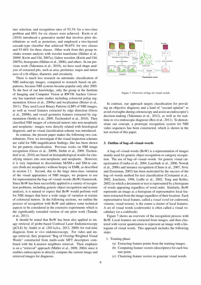
Figure 7: Overview of bag–of–visual–words.

In contrast, our approach targets classification for provid-ing an objective diagnosis and a kind of “second opinion” toavoid oversights during colonoscopy and assist an endoscopist’sdecision-making (Takemura et al., 2012), as well as for real-time in vivo endoscopic diagnosis (Rex et al., 2011). To demon-strate our concept, a prototype recognition system for NBIvideo sequences has been constructed, which is shown in thelast section of this paper.

3. Outline of bag–of–visual–words

A bag–of–visual-words (BoW) is a representation of imagesmainly used for generic object recognition or category recogni-tion. The use of bag–of–visual–words for generic visual cat-egorization (Csurka et al., 2004, Lazebnik et al., 2006, Nowaket al., 2006) and instance recognition (Chum et al., 2007, Sivicand Zisserman, 2003) has been motivated by the success of thebag–of–words method for text classification (Cristianini et al.,2002, Joachims, 1998, Lodhi et al., 2002, Tong and Koller,2002) in which a document or text is represented by a histogramof words appearing regardless of word order. Similarly, BoWrepresents an image as a histogram of representative local fea-tures extracted from the image regardless of their location. Eachrepresentative local feature, called a visual word (or codeword,visterm, visual texton), is the center a cluster of local features.A set of visual words (codewords) is often called a visual vo-cabulary (or a codebook).

Figure 7 shows an overview of the recognition process withBoW. Local features are extracted from images, and then clus-tered with vector quantization to represent an image with a his-togram of visual words. This approach includes the followingsteps:

1. Training phase(a) Extracting feature points from the training images.(b) Computing feature vectors (descriptors) for each fea-

ture point.(c) Clustering feature vectors to generate visual words.

6

(d) Representing each training image as a histogram ofvisual words.

(e) Training classifiers with the histograms of the train-ing images.

2. Test phase(a) Extracting feature points from a test image.(b) Computing feature vectors (descriptors) for each fea-

ture point.(c) Representing the test image as a histogram of visual

words.(d) Classifying the test image based on its histogram.

BoW can be divided into three main components: detectionand description of local features, visual word representation,and classification.

Detection and description of local features is the first stepwhere information is extracted from the images in the form offeature vectors. This step can be further divided into two steps:detection, or sampling (detecting the location where the fea-tures are to be extracted), and description (how the featuresare to be represented). In the next section, we focus on theScale Invariant Feature Transform (SIFT) (Lowe, 1999, 2004),which is a standard feature descriptor and known to performbetter (Mikolajczyk and Schmid, 2003, 2005) than other fea-tures such as PCA-SIFT (Ke and Sukthankar, 2004), for ex-ample. For detection, both the Difference-of-Gaussians (DoG)detector (Lowe, 1999, 2004) and grid sampling (Bosch et al.,2007, Fei-Fei and Perona, 2005, Nowak et al., 2006) are inves-tigated in this paper. Other detectors (Tuytelaars and Mikola-jczyk, 2007) such as Harris (Harris and Stephens, 1988), Harris-Laplace (Mikolajczyk and Schmid, 2004) and dense interestpoints (Tuytelaars, 2010) are also good alternatives to DoG, andinvestigating them is left for future work. SURF (Bay et al.,2008, 2006) is known to be faster than SIFT in detection speed,however, a GPU implementation of SIFT is available (Wu),and the speed of detection depends on the sampling strategy.We have seen in preliminary experiments that grid sampling ofSIFT is reasonably fast.

Visual word representation involves clustering of the ex-tracted local features for finding the visual words (the clustercenters), and histogram representation of the images. For clus-tering a large number of local features, hierarchical k-means(Nister and Stewenius, 2006) has been widely used for repre-senting a vocabulary tree. From the viewpoint that the his-togram of visual words can be considered as a representationof the local feature distributions, many vocabulary-based ap-proaches (Amores, 2010) and variants have been recently pro-posed, such as Gaussian Mixture Model (GMM) (Campbellet al., 2006, Farquhar et al., 2005, Perronnin, 2008, Perronninet al., 2006, Zhou et al., 2008), kernel density estimation (vanGemert et al., 2008), soft assigning (Philbin et al., 2008) andglobal Gaussian approach (Nakayama et al., 2010). In this pa-per, we employ a simple vocabulary-based approach as it has alower computational cost than the other methods, and investi-gate two types of histogram representations.

Classification is used to classify the test image based onits histogram representation. In this paper, Support Vector

Machine (SVM) (John Shawe-Taylor, 2000, Scholkopf andSmola, 2002, Steinwart and Christmann, 2008, Vapnik, 1998)is used with different kernel types. Other classifiers, such asNaive Bayes (Bishop, 2006, Csurka et al., 2004), Probabilis-tic Latent Semantic Analysis (pLSA) (Hofmann, 1999, Qiu andYanai, 2008, Yanai and Qiu, 2009), or Multiple Kernel Learn-ing (Joutou and Yanai, 2009, Sonnenburg et al., 2006) have alsobeen used for category recognition.

4. Technical Details

In this section, we describe some technical aspects exploredin the experiments for classifying NBI images based on the NBImagnification finding by using the BoW representation.

4.1. Local features

4.1.1. DoG–SIFTSIFT (Lowe, 1999, 2004) is a local feature descriptor invari-

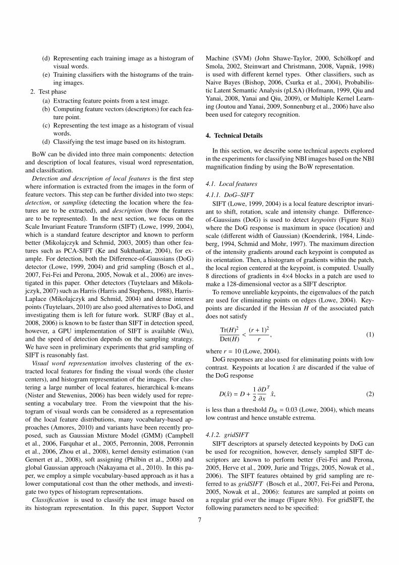
ant to shift, rotation, scale and intensity change. Difference-of-Gaussians (DoG) is used to detect keypoints (Figure 8(a))where the DoG response is maximum in space (location) andscale (different width of Gaussian) (Koenderink, 1984, Linde-berg, 1994, Schmid and Mohr, 1997). The maximum directionof the intensity gradients around each keypoint is computed asits orientation. Then, a histogram of gradients within the patch,the local region centered at the keypoint, is computed. Usually8 directions of gradients in 4×4 blocks in a patch are used tomake a 128-dimensional vector as a SIFT descriptor.

To remove unreliable keypoints, the eigenvalues of the patchare used for eliminating points on edges (Lowe, 2004). Key-points are discarded if the Hessian H of the associated patchdoes not satisfy

Tr(H)2

Det(H)<

(r + 1)2

r, (1)

where r = 10 (Lowe, 2004).DoG responses are also used for eliminating points with low

contrast. Keypoints at location x are discarded if the value ofthe DoG response

D(x) = D +12∂D∂x

T

x, (2)

is less than a threshold Dth = 0.03 (Lowe, 2004), which meanslow contrast and hence unstable extrema.

4.1.2. gridSIFTSIFT descriptors at sparsely detected keypoints by DoG can

be used for recognition, however, densely sampled SIFT de-scriptors are known to perform better (Fei-Fei and Perona,2005, Herve et al., 2009, Jurie and Triggs, 2005, Nowak et al.,2006). The SIFT features obtained by grid sampling are re-ferred to as gridSIFT (Bosch et al., 2007, Fei-Fei and Perona,2005, Nowak et al., 2006): features are sampled at points ona regular grid over the image (Figure 8(b)). For gridSIFT, thefollowing parameters need to be specified:

7

(a) (b)

Figure 8: DoG and grid sampling of features. (a) keypoints detected by DoG.(b) grid sampling.

Figure 9: Scale in gridSIFT.

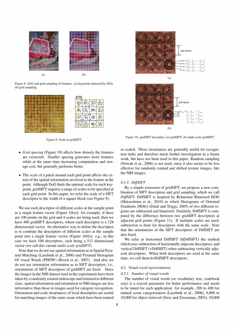
• Grid spacing (Figure 10) affects how densely the featuresare extracted. Smaller spacing generates more featureswhile at the same time increasing computation and stor-age cost, but generally performs better.

• The scale of a patch around each grid point affects the ex-tent of the spatial information involved in the feature at thepoint. Although DoG finds the optimal scale for each key-point, gridSIFT requires a range of scales to be specified ateach grid point. In this paper, we refer the scale of a SIFTdescriptor to the width of a square block (see Figure 9).

We use each descriptor of different scales at the sample pointas a single feature vector (Figure 10(a)): for example, if thereare 100 points on the grid and 4 scales are being used, then wehave 400 gridSIFT descriptors, where each descriptor is a 128dimensional vector. An alternative way to define the descriptoris to combine the descriptors of different scales at the samplepoint into a single feature vector (Figure 10(b)): e.g., in thiscase we have 100 descriptors, each being a 512 dimensionalvector (we call this variant multi-scale gridSIFT).

Note that we do not use spatial information as in Spatial Pyra-mid Matching (Lazebnik et al., 2006) and Pyramid HistogramOf visual Words (PHOW) (Bosch et al., 2007). And also wedo not use orientation information as in SIFT descriptors; i.e.,orientations of SIFT descriptors of gridSIFT are fixed. Sincethe images in the NBI dataset used in the experiments have beentaken by a randomly rotated endoscope and trimmed to differentsizes, spatial information and orientation in NBI images are lessinformative than those in images used for category recognition.Orientation and scale invariances of local descriptors are usefulfor matching images of the same scene which have been rotated

(a)

(b)

Figure 10: gridSIFT descriptor. (a) gridSIFT. (b) multi-scale gridSIFT.

or scaled. Those invariances are generally useful for recogni-tion tasks and therefore merit further investigation in a futurework, but have not been used in this paper. Random sampling(Nowak et al., 2006) is not used, since it also seems to be lesseffective for randomly rotated and shifted texture images, likethe NBI images.

4.1.3. DiffSIFTBy a simple extension of gridSIFT, we propose a new com-

bination of SIFT descriptors and grid sampling, which we callDiffSIFT. DiffSIFT is inspired by Relational Binarized HOG(Matsushima et al., 2010) in which Histograms of OrientedGradients (HOG) (Dalal and Triggs, 2005) of two different re-gions are subtracted and binarized. Similarly, DiffSIFT is com-puted by the difference between two gridSIFT descriptors atadjacent grid points (Figure 11). If multiple scales are used,subtraction is done for descriptors with the same scale. Notethat the orientations of the SIFT descriptors of DiffSIFT arealso fixed.

We refer as horizontal DiffSIFT (hDiffSIFT) the methodwhich uses subtraction of horizontally adjacent descriptors, andvertical DiffSIFT (vDiffSIFT) when subtracting vertically adja-cent descriptors. When both descriptors are used at the sametime, we call them hvDiffSIFT descriptors.

4.2. Visual word representation

4.2.1. Number of visual wordsThe number of visual words (or vocabulary size, codebook

size) is a crucial parameter for better performance and needsto be tuned for each application: for example, 200 to 400 fornatural scene categorization (Lazebnik et al., 2006), 6,000 to10,000 for object retrieval (Sivic and Zisserman, 2003), 10,000

8

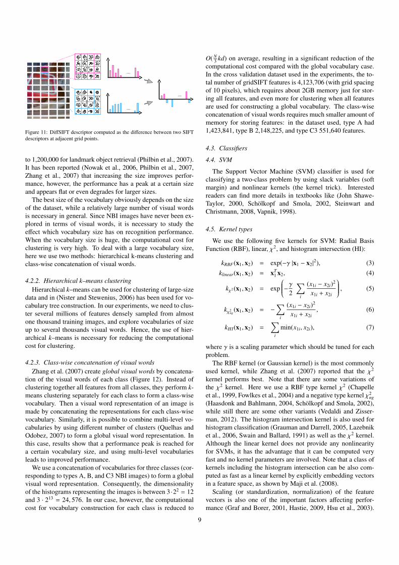
Figure 11: DiffSIFT descriptor computed as the difference between two SIFTdescriptors at adjacent grid points.

to 1,200,000 for landmark object retrieval (Philbin et al., 2007).It has been reported (Nowak et al., 2006, Philbin et al., 2007,Zhang et al., 2007) that increasing the size improves perfor-mance, however, the performance has a peak at a certain sizeand appears flat or even degrades for larger sizes.

The best size of the vocabulary obviously depends on the sizeof the dataset, while a relatively large number of visual wordsis necessary in general. Since NBI images have never been ex-plored in terms of visual words, it is necessary to study theeffect which vocabulary size has on recognition performance.When the vocabulary size is huge, the computational cost forclustering is very high. To deal with a large vocabulary size,here we use two methods: hierarchical k-means clustering andclass-wise concatenation of visual words.

4.2.2. Hierarchical k–means clusteringHierarchical k–means can be used for clustering of large-size

data and in (Nister and Stewenius, 2006) has been used for vo-cabulary tree construction. In our experiments, we need to clus-ter several millions of features densely sampled from almostone thousand training images, and explore vocabularies of sizeup to several thousands visual words. Hence, the use of hier-archical k–means is necessary for reducing the computationalcost for clustering.

4.2.3. Class-wise concatenation of visual wordsZhang et al. (2007) create global visual words by concatena-

tion of the visual words of each class (Figure 12). Instead ofclustering together all features from all classes, they perform k-means clustering separately for each class to form a class-wisevocabulary. Then a visual word representation of an image ismade by concatenating the representations for each class-wisevocabulary. Similarly, it is possible to combine multi-level vo-cabularies by using different number of clusters (Quelhas andOdobez, 2007) to form a global visual word representation. Inthis case, results show that a performance peak is reached fora certain vocabulary size, and using multi-level vocabulariesleads to improved performance.

We use a concatenation of vocabularies for three classes (cor-responding to types A, B, and C3 NBI images) to form a globalvisual word representation. Consequently, the dimensionalityof the histograms representing the images is between 3 ·22 = 12and 3 · 213 = 24, 576. In our case, however, the computationalcost for vocabulary construction for each class is reduced to

O( N3 kd) on average, resulting in a significant reduction of the

computational cost compared with the global vocabulary case.In the cross validation dataset used in the experiments, the to-tal number of gridSIFT features is 4,123,706 (with grid spacingof 10 pixels), which requires about 2GB memory just for stor-ing all features, and even more for clustering when all featuresare used for constructing a global vocabulary. The class-wiseconcatenation of visual words requires much smaller amount ofmemory for storing features: in the dataset used, type A had1,423,841, type B 2,148,225, and type C3 551,640 features.

4.3. Classifiers

4.4. SVM

The Support Vector Machine (SVM) classifier is used forclassifying a two-class problem by using slack variables (softmargin) and nonlinear kernels (the kernel trick). Interestedreaders can find more details in textbooks like (John Shawe-Taylor, 2000, Scholkopf and Smola, 2002, Steinwart andChristmann, 2008, Vapnik, 1998).

4.5. Kernel types

We use the following five kernels for SVM: Radial BasisFunction (RBF), linear, χ2, and histogram intersection (HI):

kRBF(x1, x2) = exp(−γ |x1 − x2|2), (3)

klinear(x1, x2) = xT1 x2, (4)

kχ2 (x1, x2) = exp

−γ2 ∑i

(x1i − x2i)2

x1i + x2i

, (5)

kχ2ng

(x1, x2) = −∑

i

(x1i − x2i)2

x1i + x2i, (6)

kHI(x1, x2) =∑

i

min(x1i, x2i), (7)

where γ is a scaling parameter which should be tuned for eachproblem.

The RBF kernel (or Gaussian kernel) is the most commonlyused kernel, while Zhang et al. (2007) reported that the χ2

kernel performs best. Note that there are some variations ofthe χ2 kernel. Here we use a RBF type kernel χ2 (Chapelleet al., 1999, Fowlkes et al., 2004) and a negative type kernel χ2

ng(Haasdonk and Bahlmann, 2004, Scholkopf and Smola, 2002),while still there are some other variants (Vedaldi and Zisser-man, 2012). The histogram intersection kernel is also used forhistogram classification (Grauman and Darrell, 2005, Lazebniket al., 2006, Swain and Ballard, 1991) as well as the χ2 kernel.Although the linear kernel does not provide any nonlinearityfor SVMs, it has the advantage that it can be computed veryfast and no kernel parameters are involved. Note that a class ofkernels including the histogram intersection can be also com-puted as fast as a linear kernel by explicitly embedding vectorsin a feature space, as shown by Maji et al. (2008).

Scaling (or standardization, normalization) of the featurevectors is also one of the important factors affecting perfor-mance (Graf and Borer, 2001, Hastie, 2009, Hsu et al., 2003).

9

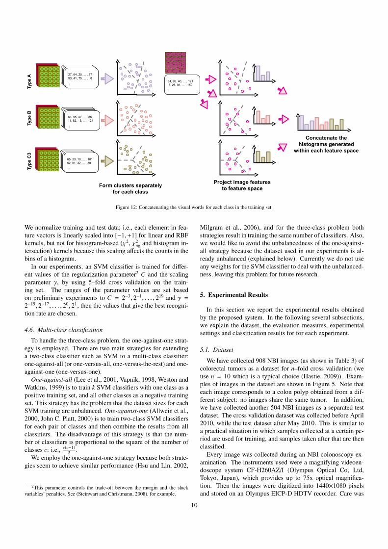
Figure 12: Concatenating the visual words for each class in the training set.

We normalize training and test data; i.e., each element in fea-ture vectors is linearly scaled into [−1,+1] for linear and RBFkernels, but not for histogram-based (χ2, χ2

ng and histogram in-tersection) kernels because this scaling affects the counts in thebins of a histogram.

In our experiments, an SVM classifier is trained for differ-ent values of the regularization parameter2 C and the scalingparameter γ, by using 5–fold cross validation on the train-ing set. The ranges of the parameter values are set basedon preliminary experiments to C = 2−3, 2−1, . . . , 219 and γ =

2−19, 2−17, . . . , 20, 21, then the values that give the best recogni-tion rate are chosen.

4.6. Multi-class classification

To handle the three-class problem, the one-against-one strat-egy is employed. There are two main strategies for extendinga two-class classifier such as SVM to a multi-class classifier:one-against-all (or one-versus-all, one-versus-the-rest) and one-against-one (one-versus-one).

One-against-all (Lee et al., 2001, Vapnik, 1998, Weston andWatkins, 1999) is to train k SVM classifiers with one class as apositive training set, and all other classes as a negative trainingset. This strategy has the problem that the dataset sizes for eachSVM training are unbalanced. One-against-one (Allwein et al.,2000, John C. Platt, 2000) is to train two-class SVM classifiersfor each pair of classes and then combine the results from allclassifiers. The disadvantage of this strategy is that the num-ber of classifiers is proportional to the square of the number ofclasses c: i.e., c(c−1)

2 .We employ the one-against-one strategy because both strate-

gies seem to achieve similar performance (Hsu and Lin, 2002,

2This parameter controls the trade-off between the margin and the slackvariables’ penalties. See (Steinwart and Christmann, 2008), for example.

Milgram et al., 2006), and for the three-class problem bothstrategies result in training the same number of classifiers. Also,we would like to avoid the unbalancedness of the one-against-all strategy because the dataset used in our experiments is al-ready unbalanced (explained below). Currently we do not useany weights for the SVM classifier to deal with the unbalanced-ness, leaving this problem for future research.

5. Experimental Results

In this section we report the experimental results obtainedby the proposed system. In the following several subsections,we explain the dataset, the evaluation measures, experimentalsettings and classification results for for each experiment.

5.1. Dataset

We have collected 908 NBI images (as shown in Table 3) ofcolorectal tumors as a dataset for n–fold cross validation (weuse n = 10 which is a typical choice (Hastie, 2009)). Exam-ples of images in the dataset are shown in Figure 5. Note thateach image corresponds to a colon polyp obtained from a dif-ferent subject: no images share the same tumor. In addition,we have collected another 504 NBI images as a separated testdataset. The cross validation dataset was collected before April2010, while the test dataset after May 2010. This is similar toa practical situation in which samples collected at a certain pe-riod are used for training, and samples taken after that are thenclassified.

Every image was collected during an NBI colonoscopy ex-amination. The instruments used were a magnifying videoen-doscope system CF-H260AZ/I (Olympus Optical Co, Ltd,Tokyo, Japan), which provides up to 75x optical magnifica-tion. Then the images were digitized into 1440×1080 pixelsand stored on an Olympus EICP-D HDTV recorder. Care was

10

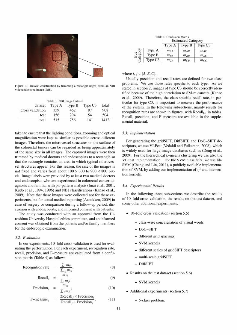
Figure 13: Dataset construction by trimming a rectangle (right) from an NBIvideoendoscope image (left).

Table 3: NBI image Datasetdataset Type A Type B Type C3 total

cross validation 359 462 87 908test 156 294 54 504

total 515 756 141 1412

taken to ensure that the lighting conditions, zooming and opticalmagnification were kept as similar as possible across differentimages. Therefore, the microvessel structures on the surface ofthe colorectal tumors can be regarded as being approximatelyof the same size in all images. The captured images were thentrimmed by medical doctors and endoscopists to a rectangle sothat the rectangle contains an area in which typical microves-sel structures appear. For this reason, the size of the images isnot fixed and varies from about 100 × 300 to 900 × 800 pix-els. Image labels were provided by at least two medical doctorsand endoscopists who are experienced in colorectal cancer di-agnosis and familiar with pit–pattern analysis (Imai et al., 2001,Kudo et al., 1994, 1996) and NBI classifications (Kanao et al.,2009). Note that these images were collected not for these ex-periments, but for actual medical reporting (Aabakken, 2009) incase of surgery or comparison during a follow-up period, dis-cussion with endoscopists, and informed consent with patients.

The study was conducted with an approval from the Hi-roshima University Hospital ethics committee, and an informedconsent was obtained from the patients and/or family membersfor the endoscopic examination.

5.2. EvaluationIn our experiments, 10–fold cross validation is used for eval-

uating the performance. For each experiment, recognition rate,recall, precision, and F–measure are calculated from a confu-sion matrix (Table 4) as follows:

Recognition rate =

∑i mii∑

i, j mi j, (8)

Recall j =m j j∑i m ji

, (9)

Precision j =m j j∑j m ji

, (10)

F–measure j =2Recall j × Precision j

Recall j + Precision j, (11)

Table 4: Confusion MatrixEstimated Category


True

Cat

egor

y Type A mAA mAB mAC

Type B mBA mBB mBC

Type C3 mCA mCB mCC

where i, j ∈ {A, B,C}.Usually precision and recall rates are defined for two-class

problems. We use those rates specific to each type. As westated in section 2, images of type C3 should be correctly iden-tified because of the high correlation to SM-m cancers (Kanaoet al., 2009). Therefore, the class-specific recall rate, in par-ticular for type C3, is important to measure the performanceof the system. In the following subsections, mainly results forrecognition rates are shown in figures, with RecallC3 in tables.Recall, precision, and F–measure are available in the supple-mental material.

5.3. Implementation

For generating the gridSIFT, DiffSIFT, and DoG–SIFT de-scriptors, we use VLFeat (Vedaldi and Fulkerson, 2008), whichis widely used for large image databases such as (Deng et al.,2009). For the hierarchical k–means clustering we use also theVLFeat implementation. For the SVM classifiers, we use lib-SVM (Chang and Lin, 2011), a publicly available implementa-tion of SVM, by adding our implementation of χ2 and intersec-tion kernels.

5.4. Experimental Results

In the following three subsections we describe the resultsof 10–fold cross validation, the results on the test dataset, andsome other additional experiments:

• 10–fold cross validation (section 5.5)

– class-wise concatenation of visual words

– DoG–SIFT

– different grid spacings

– SVM kernels

– different scales of gridSIFT descriptors

– multi-scale gridSIFT

– DiffSIFT

• Results on the test dataset (section 5.6)

– SVM kernels

• Additional experiments (section 5.7)

– 5-class problem.

11

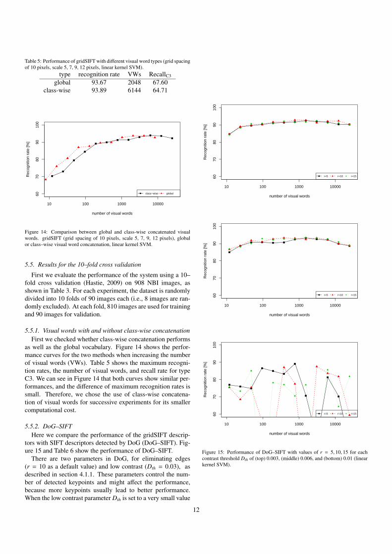
Table 5: Performance of gridSIFT with different visual word types (grid spacingof 10 pixels, scale 5, 7, 9, 12 pixels, linear kernel SVM).

type recognition rate VWs RecallC3

global 93.67 2048 67.60class-wise 93.89 6144 64.71

10 100 1000 10000

6070

8090

100

number of visual words

Rec

ogni

tion

rate

[%]

class−wise global

Figure 14: Comparison between global and class-wise concatenated visualwords. gridSIFT (grid spacing of 10 pixels, scale 5, 7, 9, 12 pixels), globalor class–wise visual word concatenation, linear kernel SVM.

5.5. Results for the 10–fold cross validation

First we evaluate the performance of the system using a 10–fold cross validation (Hastie, 2009) on 908 NBI images, asshown in Table 3. For each experiment, the dataset is randomlydivided into 10 folds of 90 images each (i.e., 8 images are ran-domly excluded). At each fold, 810 images are used for trainingand 90 images for validation.

5.5.1. Visual words with and without class-wise concatenationFirst we checked whether class-wise concatenation performs

as well as the global vocabulary. Figure 14 shows the perfor-mance curves for the two methods when increasing the numberof visual words (VWs). Table 5 shows the maximum recogni-tion rates, the number of visual words, and recall rate for typeC3. We can see in Figure 14 that both curves show similar per-formances, and the difference of maximum recognition rates issmall. Therefore, we chose the use of class-wise concatena-tion of visual words for successive experiments for its smallercomputational cost.

5.5.2. DoG–SIFTHere we compare the performance of the gridSIFT descrip-

tors with SIFT descriptors detected by DoG (DoG–SIFT). Fig-ure 15 and Table 6 show the performance of DoG–SIFT.

There are two parameters in DoG, for eliminating edges(r = 10 as a default value) and low contrast (Dth = 0.03), asdescribed in section 4.1.1. These parameters control the num-ber of detected keypoints and might affect the performance,because more keypoints usually lead to better performance.When the low contrast parameter Dth is set to a very small value

10 100 1000 10000

6070

8090

100


Rec

ogni

tion

rate

[%]

r=5 r=10 r=15

10 100 1000 10000

6070

8090

100


Rec

ogni

tion

rate

[%]

r=5 r=10 r=15

10 100 1000 10000

6070

8090

100


Rec

ogni

tion

rate

[%]

r=5 r=10 r=15

Figure 15: Performance of DoG–SIFT with values of r = 5, 10, 15 for eachcontrast threshold Dth of (top) 0.003, (middle) 0.006, and (bottom) 0.01 (linearkernel SVM).

12

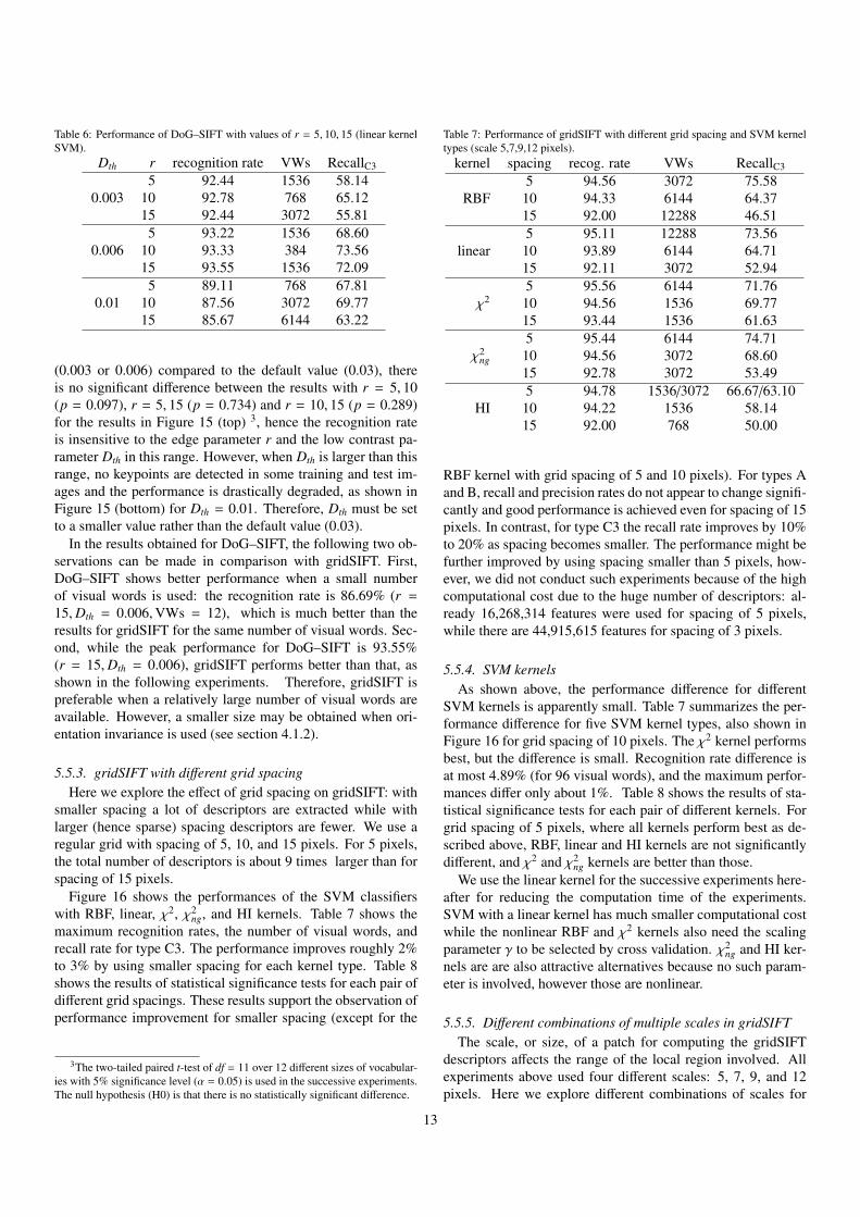
Table 6: Performance of DoG–SIFT with values of r = 5, 10, 15 (linear kernelSVM).

Dth r recognition rate VWs RecallC3

0.0035 92.44 1536 58.14

10 92.78 768 65.1215 92.44 3072 55.81

0.0065 93.22 1536 68.60

10 93.33 384 73.5615 93.55 1536 72.09

0.015 89.11 768 67.81

10 87.56 3072 69.7715 85.67 6144 63.22

(0.003 or 0.006) compared to the default value (0.03), thereis no significant difference between the results with r = 5, 10(p = 0.097), r = 5, 15 (p = 0.734) and r = 10, 15 (p = 0.289)for the results in Figure 15 (top) 3, hence the recognition rateis insensitive to the edge parameter r and the low contrast pa-rameter Dth in this range. However, when Dth is larger than thisrange, no keypoints are detected in some training and test im-ages and the performance is drastically degraded, as shown inFigure 15 (bottom) for Dth = 0.01. Therefore, Dth must be setto a smaller value rather than the default value (0.03).

In the results obtained for DoG–SIFT, the following two ob-servations can be made in comparison with gridSIFT. First,DoG–SIFT shows better performance when a small numberof visual words is used: the recognition rate is 86.69% (r =

15,Dth = 0.006,VWs = 12), which is much better than theresults for gridSIFT for the same number of visual words. Sec-ond, while the peak performance for DoG–SIFT is 93.55%(r = 15,Dth = 0.006), gridSIFT performs better than that, asshown in the following experiments. Therefore, gridSIFT ispreferable when a relatively large number of visual words areavailable. However, a smaller size may be obtained when ori-entation invariance is used (see section 4.1.2).

5.5.3. gridSIFT with different grid spacingHere we explore the effect of grid spacing on gridSIFT: with

smaller spacing a lot of descriptors are extracted while withlarger (hence sparse) spacing descriptors are fewer. We use aregular grid with spacing of 5, 10, and 15 pixels. For 5 pixels,the total number of descriptors is about 9 times larger than forspacing of 15 pixels.

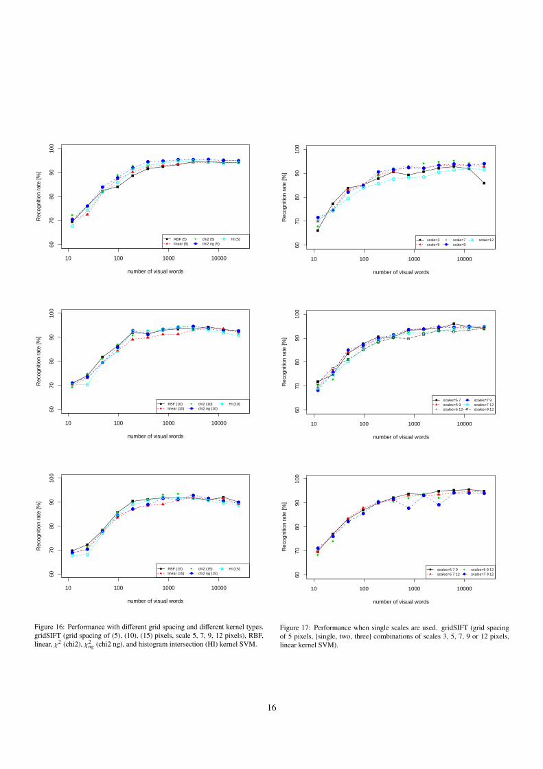
Figure 16 shows the performances of the SVM classifierswith RBF, linear, χ2, χ2

ng, and HI kernels. Table 7 shows themaximum recognition rates, the number of visual words, andrecall rate for type C3. The performance improves roughly 2%to 3% by using smaller spacing for each kernel type. Table 8shows the results of statistical significance tests for each pair ofdifferent grid spacings. These results support the observation ofperformance improvement for smaller spacing (except for the

3The two-tailed paired t-test of df = 11 over 12 different sizes of vocabular-ies with 5% significance level (α = 0.05) is used in the successive experiments.The null hypothesis (H0) is that there is no statistically significant difference.

Table 7: Performance of gridSIFT with different grid spacing and SVM kerneltypes (scale 5,7,9,12 pixels).

kernel spacing recog. rate VWs RecallC3

RBF5 94.56 3072 75.58

10 94.33 6144 64.3715 92.00 12288 46.51

linear5 95.11 12288 73.56

10 93.89 6144 64.7115 92.11 3072 52.94

χ25 95.56 6144 71.76

10 94.56 1536 69.7715 93.44 1536 61.63

χ2ng

5 95.44 6144 74.7110 94.56 3072 68.6015 92.78 3072 53.49

HI5 94.78 1536/3072 66.67/63.10

10 94.22 1536 58.1415 92.00 768 50.00

RBF kernel with grid spacing of 5 and 10 pixels). For types Aand B, recall and precision rates do not appear to change signifi-cantly and good performance is achieved even for spacing of 15pixels. In contrast, for type C3 the recall rate improves by 10%to 20% as spacing becomes smaller. The performance might befurther improved by using spacing smaller than 5 pixels, how-ever, we did not conduct such experiments because of the highcomputational cost due to the huge number of descriptors: al-ready 16,268,314 features were used for spacing of 5 pixels,while there are 44,915,615 features for spacing of 3 pixels.

5.5.4. SVM kernelsAs shown above, the performance difference for different

SVM kernels is apparently small. Table 7 summarizes the per-formance difference for five SVM kernel types, also shown inFigure 16 for grid spacing of 10 pixels. The χ2 kernel performsbest, but the difference is small. Recognition rate difference isat most 4.89% (for 96 visual words), and the maximum perfor-mances differ only about 1%. Table 8 shows the results of sta-tistical significance tests for each pair of different kernels. Forgrid spacing of 5 pixels, where all kernels perform best as de-scribed above, RBF, linear and HI kernels are not significantlydifferent, and χ2 and χ2

ng kernels are better than those.We use the linear kernel for the successive experiments here-

after for reducing the computation time of the experiments.SVM with a linear kernel has much smaller computational costwhile the nonlinear RBF and χ2 kernels also need the scalingparameter γ to be selected by cross validation. χ2

ng and HI ker-nels are are also attractive alternatives because no such param-eter is involved, however those are nonlinear.

5.5.5. Different combinations of multiple scales in gridSIFTThe scale, or size, of a patch for computing the gridSIFT

descriptors affects the range of the local region involved. Allexperiments above used four different scales: 5, 7, 9, and 12pixels. Here we explore different combinations of scales for

13

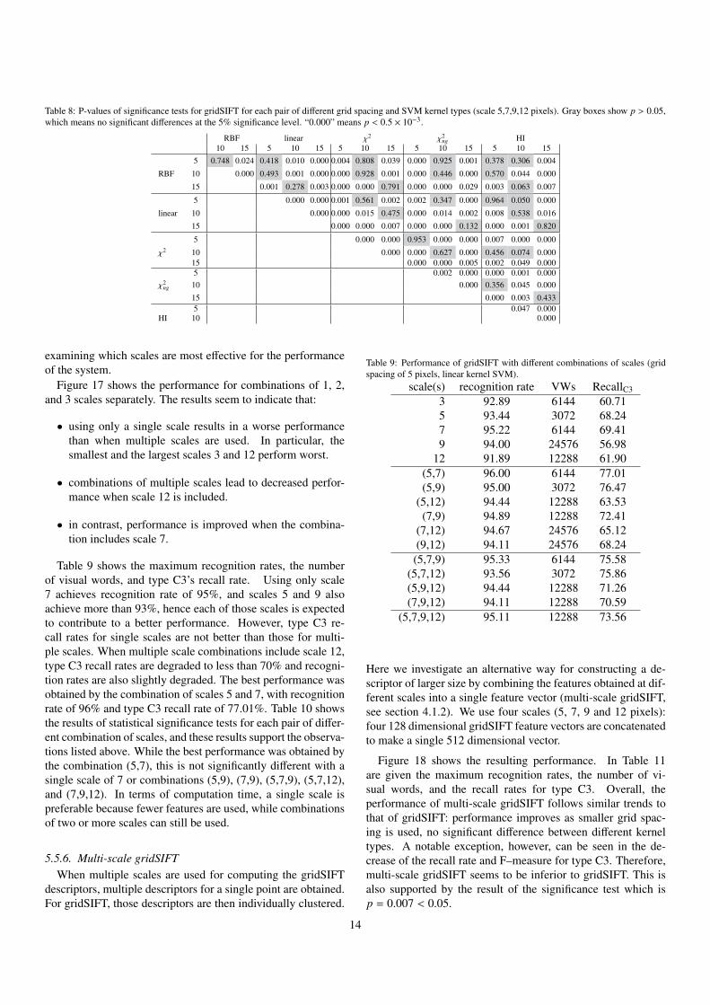
Table 8: P-values of significance tests for gridSIFT for each pair of different grid spacing and SVM kernel types (scale 5,7,9,12 pixels). Gray boxes show p > 0.05,which means no significant differences at the 5% significance level. “0.000” means p < 0.5 × 10−3.

RBF linear χ2 χ2ng HI

10 15 5 10 15 5 10 15 5 10 15 5 10 15

5 0.748 0.024 0.418 0.010 0.000 0.004 0.808 0.039 0.000 0.925 0.001 0.378 0.306 0.004

RBF 10 0.000 0.493 0.001 0.000 0.000 0.928 0.001 0.000 0.446 0.000 0.570 0.044 0.000

15 0.001 0.278 0.003 0.000 0.000 0.791 0.000 0.000 0.029 0.003 0.063 0.007

5 0.000 0.000 0.001 0.561 0.002 0.002 0.347 0.000 0.964 0.050 0.000

linear 10 0.000 0.000 0.015 0.475 0.000 0.014 0.002 0.008 0.538 0.016

15 0.000 0.000 0.007 0.000 0.000 0.132 0.000 0.001 0.820

5 0.000 0.000 0.953 0.000 0.000 0.007 0.000 0.000

χ2 10 0.000 0.000 0.627 0.000 0.456 0.074 0.00015 0.000 0.000 0.005 0.002 0.049 0.0005 0.002 0.000 0.000 0.001 0.000

χ2ng 10 0.000 0.356 0.045 0.000

15 0.000 0.003 0.4335 0.047 0.000

HI 10 0.000

examining which scales are most effective for the performanceof the system.

Figure 17 shows the performance for combinations of 1, 2,and 3 scales separately. The results seem to indicate that:

• using only a single scale results in a worse performancethan when multiple scales are used. In particular, thesmallest and the largest scales 3 and 12 perform worst.

• combinations of multiple scales lead to decreased perfor-mance when scale 12 is included.

• in contrast, performance is improved when the combina-tion includes scale 7.

Table 9 shows the maximum recognition rates, the numberof visual words, and type C3’s recall rate. Using only scale7 achieves recognition rate of 95%, and scales 5 and 9 alsoachieve more than 93%, hence each of those scales is expectedto contribute to a better performance. However, type C3 re-call rates for single scales are not better than those for multi-ple scales. When multiple scale combinations include scale 12,type C3 recall rates are degraded to less than 70% and recogni-tion rates are also slightly degraded. The best performance wasobtained by the combination of scales 5 and 7, with recognitionrate of 96% and type C3 recall rate of 77.01%. Table 10 showsthe results of statistical significance tests for each pair of differ-ent combination of scales, and these results support the observa-tions listed above. While the best performance was obtained bythe combination (5,7), this is not significantly different with asingle scale of 7 or combinations (5,9), (7,9), (5,7,9), (5,7,12),and (7,9,12). In terms of computation time, a single scale ispreferable because fewer features are used, while combinationsof two or more scales can still be used.

5.5.6. Multi-scale gridSIFTWhen multiple scales are used for computing the gridSIFT

descriptors, multiple descriptors for a single point are obtained.For gridSIFT, those descriptors are then individually clustered.

Table 9: Performance of gridSIFT with different combinations of scales (gridspacing of 5 pixels, linear kernel SVM).

scale(s) recognition rate VWs RecallC3

3 92.89 6144 60.715 93.44 3072 68.247 95.22 6144 69.419 94.00 24576 56.98

12 91.89 12288 61.90(5,7) 96.00 6144 77.01(5,9) 95.00 3072 76.47

(5,12) 94.44 12288 63.53(7,9) 94.89 12288 72.41

(7,12) 94.67 24576 65.12(9,12) 94.11 24576 68.24

(5,7,9) 95.33 6144 75.58(5,7,12) 93.56 3072 75.86(5,9,12) 94.44 12288 71.26(7,9,12) 94.11 12288 70.59

(5,7,9,12) 95.11 12288 73.56

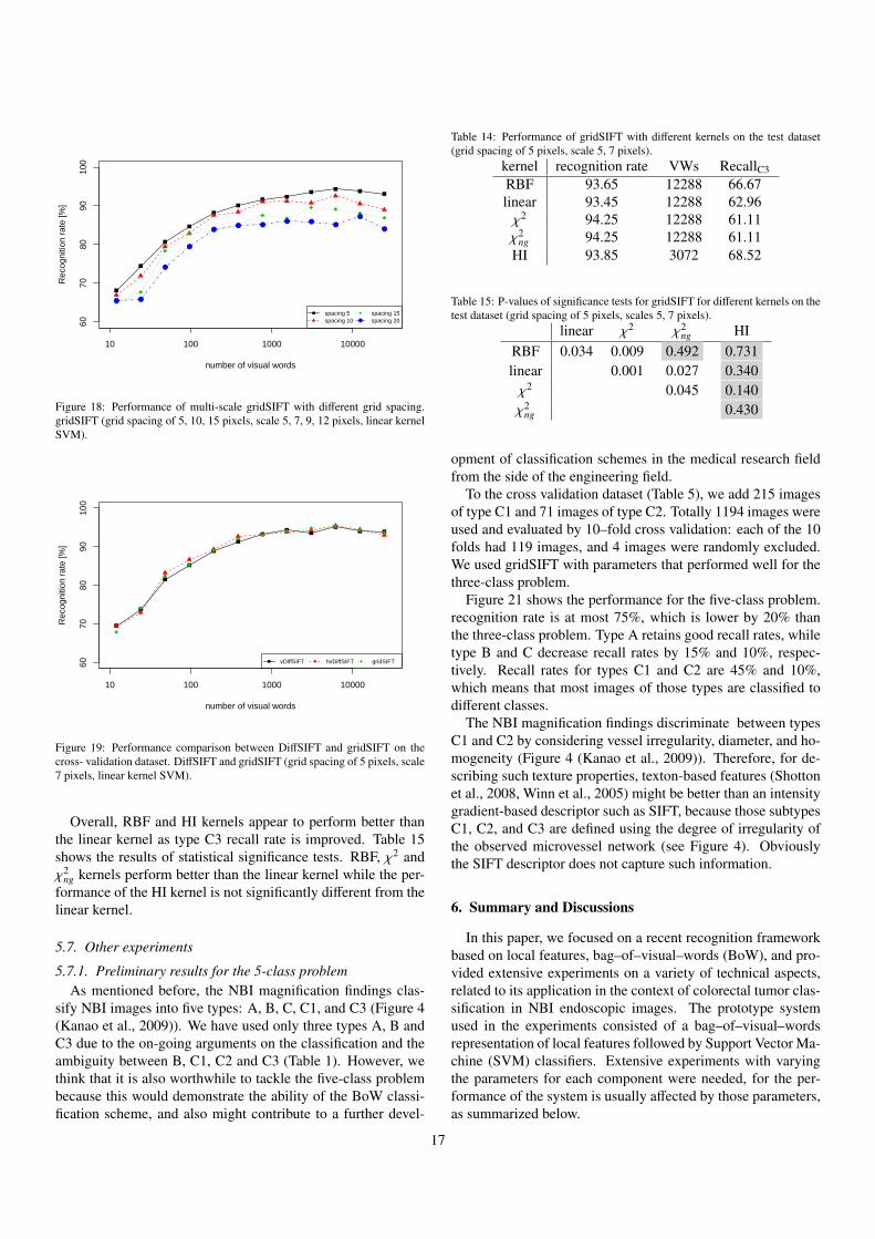
Here we investigate an alternative way for constructing a de-scriptor of larger size by combining the features obtained at dif-ferent scales into a single feature vector (multi-scale gridSIFT,see section 4.1.2). We use four scales (5, 7, 9 and 12 pixels):four 128 dimensional gridSIFT feature vectors are concatenatedto make a single 512 dimensional vector.

Figure 18 shows the resulting performance. In Table 11are given the maximum recognition rates, the number of vi-sual words, and the recall rates for type C3. Overall, theperformance of multi-scale gridSIFT follows similar trends tothat of gridSIFT: performance improves as smaller grid spac-ing is used, no significant difference between different kerneltypes. A notable exception, however, can be seen in the de-crease of the recall rate and F–measure for type C3. Therefore,multi-scale gridSIFT seems to be inferior to gridSIFT. This isalso supported by the result of the significance test which isp = 0.007 < 0.05.

14

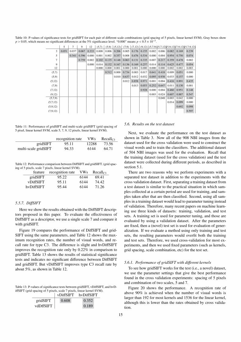
Table 10: P-values of significance tests for gridSIFT for each pair of different scale combinations (grid spacing of 5 pixels, linear kernel SVM). Gray boxes showp > 0.05, which means no significant differences at the 5% significance level. “0.000” means p < 0.5 × 10−3.

5 7 9 12 (5,7) (5,9) (5,12) (7,9) (7,12) (9,12) (5,7,9) (5,7,12)(5,9,12)(7,9,12)(5,7,9,12)

3 0.051 0.037 0.067 0.333 0.008 0.006 0.206 0.005 0.176 0.155 0.002 0.006 0.082 0.169 0.239

5 0.341 0.396 0.000 0.001 0.002 0.357 0.008 0.476 0.534 0.000 0.004 0.954 0.750 0.074

7 0.759 0.002 0.102 0.135 0.148 0.063 0.131 0.335 0.007 0.217 0.359 0.478 0.002

9 0.000 0.014 0.132 0.167 0.136 0.169 0.257 0.014 0.114 0.625 0.477 0.05412 0.000 0.000 0.001 0.000 0.001 0.000 0.000 0.000 0.002 0.002 0.003

(5,7) 0.512 0.000 0.734 0.003 0.017 0.641 0.418 0.009 0.051 0.000

(5,9) 0.010 0.637 0.012 0.032 0.095 0.938 0.033 0.157 0.000

(5,12) 0.012 0.858 0.971 0.001 0.004 0.416 0.891 0.435

(7,9) 0.013 0.053 0.252 0.647 0.011 0.130 0.001

(7,12) 0.928 0.000 0.004 0.460 0.951 0.148

(9,12) 0.003 0.024 0.607 0.887 0.547(5,7,9) 0.048 0.003 0.042 0.000

(5,7,12) 0.014 0.099 0.000

(5,9,12) 0.692 0.098

(7,9,12) 0.597

Table 11: Performance of gridSIFT and multi-scale gridSIFT (grid spacing of5 pixel, linear kernel SVM, scale 5, 7, 9, 12 pixels, linear kernel SVM).

recognition rate VWs RecallC3

gridSIFT 95.11 12288 73.56multi-scale gridSIFT 94.33 6144 64.71

Table 12: Performance comparison between DiffSIFT and gridSIFT. (grid spac-ing of 5 pixels, scale 7 pixels, linear kernel SVM).

feature recognition rate VWs RecallC3

gridSIFT 95.22 6144 69.41vDiffSIFT 95.11 6144 74.42

hvDiffSIFT 95.44 6144 71.26

5.5.7. DiffSIFT

Here we show the results obtained with the DiffSIFT descrip-tors proposed in this paper. To evaluate the effectiveness ofDiffSIFT as a descriptor, we use a single scale 7 and compare itwith gridSIFT.

Figure 19 compares the performance of DiffSIFT and grid-SIFT using the same parameters, and Table 12 shows the max-imum recognition rates, the number of visual words, and re-call rate for type C3. The difference is slight and hvDiffSIFTimproves the recognition rate only by 0.22% in comparison togridSIFT. Table 13 shows the results of statistical significancetests and indicates no significant difference between DiffSIFTand gridSIFT. But vDiffSIFT improves type C3 recall rate byabout 5%, as shown in Table 12.

Table 13: P-values of significance tests between gridSIFT, vDiffSIFT, and hvD-iffSIFT (grid spacing of 5 pixels, scale 7 pixels, linear kernel SVM).

vDiffSIFT hvDiffSIFTgridSIFT 0.608 0.352

vdDffSIFT 0.189

5.6. Results on the test dataset

Next, we evaluate the performance on the test dataset asshown in Table 3. Now all of the 908 NBI images from thedataset used for the cross validation were used to construct thevisual words and to train the classifiers. The additional datasetof 504 NBI images was used for the evaluation. Recall thatthe training dataset (used for the cross validation) and the testdataset were collected during different periods, as described insection 5.1.

There are two reasons why we perform experiments with aseparated test dataset in addition to the experiments with thecross validation dataset. First, separating a training dataset froma test dataset is similar to the practical situation in which sam-ples collected at a certain period are used for training, and sam-ples taken after that are then classified. Second, using all sam-ples in a training dataset would lead to parameter tuning insteadof validation. Therefore, many recent papers on machine learn-ing use three kinds of datasets: training, validation, and testsets. A training set is used for parameter tuning, and those areevaluated by using a validation dataset. After the parametersare fixed, then a (novel) test set is used for evaluation of gener-alization. If we evaluate a method using only training and testsets, the resulting parameters would overfit both the trainingand test sets. Therefore, we used cross-validation for most ex-periments, and then we used fixed parameters (such as kernels,grid spacing, scale combination, etc) for the test set.

5.6.1. Performance of gridSIFT with different kernelsTo see how gridSIFT works for the test (i.e., a novel) dataset,

we use the parameter settings that give the best performancefound in the cross validation experiments: spacing of 5 pixelsand combination of two scales, 5 and 7.

Figure 20 shows the performance. A recognition rate ofabove 90% is achieved when the number of visual words islarger than 192 for most kernels and 1536 for the linear kernel,although this is lower than the rates obtained by cross valida-tion.

15

10 100 1000 10000

6070

8090

100


Rec

ogni

tion

rate

[%]

●

●

●

●

●

● ● ● ● ● ● ●

●

●

●

●

●

● ●● ● ●

● ●

●

●RBF (5)linear (5)

chi2 (5)chi2 ng (5)

HI (5)

10 100 1000 10000

6070

8090

100


Rec

ogni

tion

rate

[%]

●

●

●

●

●●

●● ●

●● ●

● ●

●

●

● ● ●●

● ●●

●

●


chi2 (10)chi2 ng (10)

HI (10)

10 100 1000 10000

6070

8090

100


Rec

ogni

tion

rate

[%]

●●

●

●

●

●

● ●●

●● ●

● ●

●

●

●●

● ● ●●

●●

●


chi2 (15)chi2 ng (15)

HI (15)

Figure 16: Performance with different grid spacing and different kernel types.gridSIFT (grid spacing of (5), (10), (15) pixels, scale 5, 7, 9, 12 pixels), RBF,linear, χ2 (chi2), χ2

ng (chi2 ng), and histogram intersection (HI) kernel SVM.

10 100 1000 10000

6070

8090

100


Rec

ogni

tion

rate

[%]

●

●

●

●

●●

● ●● ● ● ●

●

●

●

●

●

● ● ●

●● ● ●

●

●scale=3scale=5

scale=7scale=9

scale=12

10 100 1000 10000

6070

8090

100


Rec

ogni

tion

rate

[%]

●

●

●

●

●●

● ●● ● ● ●

●

●

●

●

●

●● ●

●● ● ●

●

●

scales=5 7scales=5 9scales=5 12

scales=7 9scales=7 12scales=9 12

10 100 1000 10000

6070

8090

100


Rec

ogni

tion

rate

[%]

●

●

●

●

●●

●

●

●

● ● ●

●

scales=5 7 9scales=5 7 12

scales=5 9 12scales=7 9 12

Figure 17: Performance when single scales are used. gridSIFT (grid spacingof 5 pixels, {single, two, three} combinations of scales 3, 5, 7, 9 or 12 pixels,linear kernel SVM).

16

10 100 1000 10000

6070

8090

100


Rec

ogni

tion

rate

[%]

● ●

●

●

●● ●

● ●●

●

●

●

spacing 5spacing 10

spacing 15spacing 20

Figure 18: Performance of multi-scale gridSIFT with different grid spacing.gridSIFT (grid spacing of 5, 10, 15 pixels, scale 5, 7, 9, 12 pixels, linear kernelSVM).

10 100 1000 10000

6070

8090

100


Rec

ogni

tion

rate

[%]

vDiffSIFT hvDiffSIFT gridSIFT

Figure 19: Performance comparison between DiffSIFT and gridSIFT on thecross- validation dataset. DiffSIFT and gridSIFT (grid spacing of 5 pixels, scale7 pixels, linear kernel SVM).

Overall, RBF and HI kernels appear to perform better thanthe linear kernel as type C3 recall rate is improved. Table 15shows the results of statistical significance tests. RBF, χ2 andχ2

ng kernels perform better than the linear kernel while the per-formance of the HI kernel is not significantly different from thelinear kernel.

5.7. Other experiments

5.7.1. Preliminary results for the 5-class problemAs mentioned before, the NBI magnification findings clas-

sify NBI images into five types: A, B, C, C1, and C3 (Figure 4(Kanao et al., 2009)). We have used only three types A, B andC3 due to the on-going arguments on the classification and theambiguity between B, C1, C2 and C3 (Table 1). However, wethink that it is also worthwhile to tackle the five-class problembecause this would demonstrate the ability of the BoW classi-fication scheme, and also might contribute to a further devel-

Table 14: Performance of gridSIFT with different kernels on the test dataset(grid spacing of 5 pixels, scale 5, 7 pixels).

kernel recognition rate VWs RecallC3

RBF 93.65 12288 66.67linear 93.45 12288 62.96χ2 94.25 12288 61.11χ2

ng 94.25 12288 61.11HI 93.85 3072 68.52

Table 15: P-values of significance tests for gridSIFT for different kernels on thetest dataset (grid spacing of 5 pixels, scales 5, 7 pixels).

linear χ2 χ2ng HI

RBF 0.034 0.009 0.492 0.731linear 0.001 0.027 0.340χ2 0.045 0.140χ2

ng 0.430

opment of classification schemes in the medical research fieldfrom the side of the engineering field.

To the cross validation dataset (Table 5), we add 215 imagesof type C1 and 71 images of type C2. Totally 1194 images wereused and evaluated by 10–fold cross validation: each of the 10folds had 119 images, and 4 images were randomly excluded.We used gridSIFT with parameters that performed well for thethree-class problem.

Figure 21 shows the performance for the five-class problem.recognition rate is at most 75%, which is lower by 20% thanthe three-class problem. Type A retains good recall rates, whiletype B and C decrease recall rates by 15% and 10%, respec-tively. Recall rates for types C1 and C2 are 45% and 10%,which means that most images of those types are classified todifferent classes.

The NBI magnification findings discriminate between typesC1 and C2 by considering vessel irregularity, diameter, and ho-mogeneity (Figure 4 (Kanao et al., 2009)). Therefore, for de-scribing such texture properties, texton-based features (Shottonet al., 2008, Winn et al., 2005) might be better than an intensitygradient-based descriptor such as SIFT, because those subtypesC1, C2, and C3 are defined using the degree of irregularity ofthe observed microvessel network (see Figure 4). Obviouslythe SIFT descriptor does not capture such information.

6. Summary and Discussions

In this paper, we focused on a recent recognition frameworkbased on local features, bag–of–visual–words (BoW), and pro-vided extensive experiments on a variety of technical aspects,related to its application in the context of colorectal tumor clas-sification in NBI endoscopic images. The prototype systemused in the experiments consisted of a bag–of–visual–wordsrepresentation of local features followed by Support Vector Ma-chine (SVM) classifiers. Extensive experiments with varyingthe parameters for each component were needed, for the per-formance of the system is usually affected by those parameters,as summarized below.

17

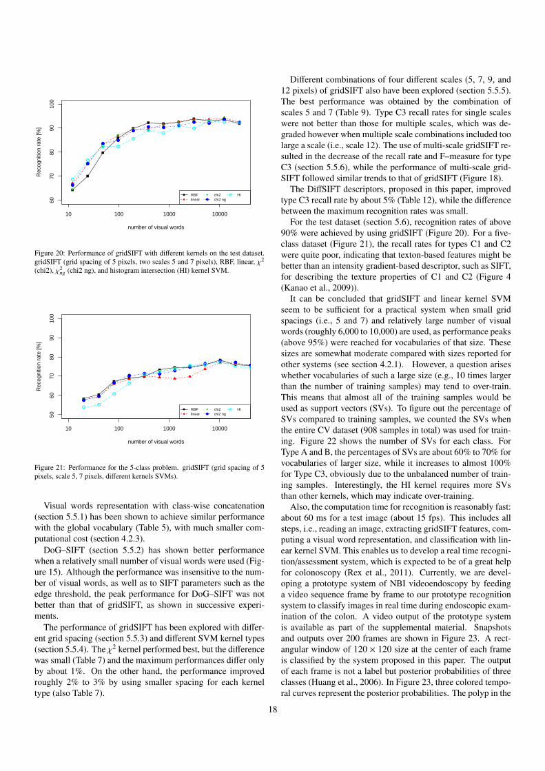
10 100 1000 10000

6070

8090

100


Rec

ogni

tion

rate

[%]

●

●

●●

●● ●

●● ●

●●

●

●

● ●

●

●●

●●

● ● ●

●

●RBFlinear

chi2chi2 ng

HI

Figure 20: Performance of gridSIFT with different kernels on the test dataset.gridSIFT (grid spacing of 5 pixels, two scales 5 and 7 pixels), RBF, linear, χ2

(chi2), χ2ng (chi2 ng), and histogram intersection (HI) kernel SVM.

10 100 1000 10000

5060

7080

9010

0


Rec

ogni

tion

rate

[%]

●●

●

●● ●

●●

●● ●

●

●●

●

●

●●

●● ●

●● ●

●

●RBFlinear

chi2chi2 ng

HI

Figure 21: Performance for the 5-class problem. gridSIFT (grid spacing of 5pixels, scale 5, 7 pixels, different kernels SVMs).

Visual words representation with class-wise concatenation(section 5.5.1) has been shown to achieve similar performancewith the global vocabulary (Table 5), with much smaller com-putational cost (section 4.2.3).

DoG–SIFT (section 5.5.2) has shown better performancewhen a relatively small number of visual words were used (Fig-ure 15). Although the performance was insensitive to the num-ber of visual words, as well as to SIFT parameters such as theedge threshold, the peak performance for DoG–SIFT was notbetter than that of gridSIFT, as shown in successive experi-ments.

The performance of gridSIFT has been explored with differ-ent grid spacing (section 5.5.3) and different SVM kernel types(section 5.5.4). The χ2 kernel performed best, but the differencewas small (Table 7) and the maximum performances differ onlyby about 1%. On the other hand, the performance improvedroughly 2% to 3% by using smaller spacing for each kerneltype (also Table 7).

Different combinations of four different scales (5, 7, 9, and12 pixels) of gridSIFT also have been explored (section 5.5.5).The best performance was obtained by the combination ofscales 5 and 7 (Table 9). Type C3 recall rates for single scaleswere not better than those for multiple scales, which was de-graded however when multiple scale combinations included toolarge a scale (i.e., scale 12). The use of multi-scale gridSIFT re-sulted in the decrease of the recall rate and F–measure for typeC3 (section 5.5.6), while the performance of multi-scale grid-SIFT followed similar trends to that of gridSIFT (Figure 18).

The DiffSIFT descriptors, proposed in this paper, improvedtype C3 recall rate by about 5% (Table 12), while the differencebetween the maximum recognition rates was small.

For the test dataset (section 5.6), recognition rates of above90% were achieved by using gridSIFT (Figure 20). For a five-class dataset (Figure 21), the recall rates for types C1 and C2were quite poor, indicating that texton-based features might bebetter than an intensity gradient-based descriptor, such as SIFT,for describing the texture properties of C1 and C2 (Figure 4(Kanao et al., 2009)).

It can be concluded that gridSIFT and linear kernel SVMseem to be sufficient for a practical system when small gridspacings (i.e., 5 and 7) and relatively large number of visualwords (roughly 6,000 to 10,000) are used, as performance peaks(above 95%) were reached for vocabularies of that size. Thesesizes are somewhat moderate compared with sizes reported forother systems (see section 4.2.1). However, a question ariseswhether vocabularies of such a large size (e.g., 10 times largerthan the number of training samples) may tend to over-train.This means that almost all of the training samples would beused as support vectors (SVs). To figure out the percentage ofSVs compared to training samples, we counted the SVs whenthe entire CV dataset (908 samples in total) was used for train-ing. Figure 22 shows the number of SVs for each class. ForType A and B, the percentages of SVs are about 60% to 70% forvocabularies of larger size, while it increases to almost 100%for Type C3, obviously due to the unbalanced number of train-ing samples. Interestingly, the HI kernel requires more SVsthan other kernels, which may indicate over-training.

Also, the computation time for recognition is reasonably fast:about 60 ms for a test image (about 15 fps). This includes allsteps, i.e., reading an image, extracting gridSIFT features, com-puting a visual word representation, and classification with lin-ear kernel SVM. This enables us to develop a real time recogni-tion/assessment system, which is expected to be of a great helpfor colonoscopy (Rex et al., 2011). Currently, we are devel-oping a prototype system of NBI videoendoscopy by feedinga video sequence frame by frame to our prototype recognitionsystem to classify images in real time during endoscopic exam-ination of the colon. A video output of the prototype systemis available as part of the supplemental material. Snapshotsand outputs over 200 frames are shown in Figure 23. A rect-angular window of 120 × 120 size at the center of each frameis classified by the system proposed in this paper. The outputof each frame is not a label but posterior probabilities of threeclasses (Huang et al., 2006). In Figure 23, three colored tempo-ral curves represent the posterior probabilities. The polyp in the

18

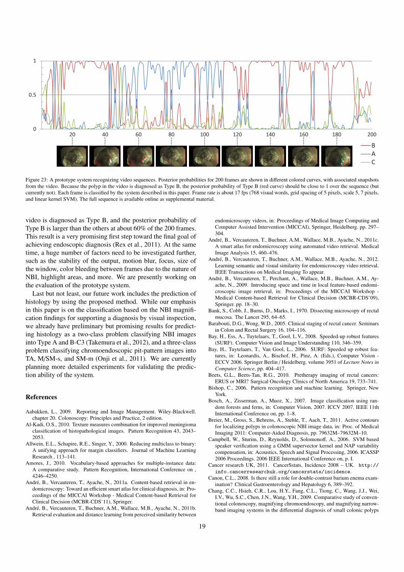
0

0.5

1

B

A

C

20 40 60 80 100 120 140 160 180 200

Figure 23: A prototype system recognizing video sequences. Posterior probabilities for 200 frames are shown in different colored curves, with associated snapshotsfrom the video. Because the polyp in the video is diagnosed as Type B, the posterior probability of Type B (red curve) should be close to 1 over the sequence (butcurrently not). Each frame is classified by the system described in this paper. Frame rate is about 17 fps (768 visual words, grid spacing of 5 pixels, scale 5, 7 pixels,and linear kernel SVM). The full sequence is available online as supplemental material.

video is diagnosed as Type B, and the posterior probability ofType B is larger than the others at about 60% of the 200 frames.This result is a very promising first step toward the final goal ofachieving endoscopic diagnosis (Rex et al., 2011). At the sametime, a huge number of factors need to be investigated further,such as the stability of the output, motion blur, focus, size ofthe window, color bleeding between frames due to the nature ofNBI, highlight areas, and more. We are presently working onthe evaluation of the prototype system.

Last but not least, our future work includes the prediction ofhistology by using the proposed method. While our emphasisin this paper is on the classification based on the NBI magnifi-cation findings for supporting a diagnosis by visual inspection,we already have preliminary but promising results for predict-ing histology as a two-class problem classifying NBI imagesinto Type A and B-C3 (Takemura et al., 2012), and a three-classproblem classifying chromoendoscopic pit-pattern images intoTA, M/SM-s, and SM-m (Onji et al., 2011). We are currentlyplanning more detailed experiments for validating the predic-tion ability of the system.

References

Aabakken, L., 2009. Reporting and Image Management. Wiley-Blackwell.chapter 20. Colonoscopy: Principles and Practice, 2 edition.

Al-Kadi, O.S., 2010. Texture measures combination for improved meningiomaclassification of histopathological images. Pattern Recognition 43, 2043–2053.

Allwein, E.L., Schapire, R.E., Singer, Y., 2000. Reducing multiclass to binary:A unifying approach for margin classifiers. Journal of Machine LearningResearch , 113–141.

Amores, J., 2010. Vocabulary-based approaches for multiple-instance data:A comparative study. Pattern Recognition, International Conference on ,4246–4250.

Andre, B., Vercauteren, T., Ayache, N., 2011a. Content-based retrieval in en-domicroscopy: Toward an efficient smart atlas for clinical diagnosis, in: Pro-ceedings of the MICCAI Workshop - Medical Content-based Retrieval forClinical Decision (MCBR-CDS’11), Springer.

Andre, B., Vercauteren, T., Buchner, A.M., Wallace, M.B., Ayache, N., 2011b.Retrieval evaluation and distance learning from perceived similarity between

endomicroscopy videos, in: Proceedings of Medical Image Computing andComputer Assisted Intervention (MICCAI), Springer, Heidelberg. pp. 297–304.

Andre, B., Vercauteren, T., Buchner, A.M., Wallace, M.B., Ayache, N., 2011c.A smart atlas for endomicroscopy using automated video retrieval. MedicalImage Analysis 15, 460–476.

Andre, B., Vercauteren, T., Buchner, A.M., Wallace, M.B., Ayache, N., 2012.Learning semantic and visual similarity for endomicroscopy video retrieval.IEEE Transactions on Medical Imaging To appear.

Andre, B., Vercauteren, T., Perchant, A., Wallace, M.B., Buchner, A.M., Ay-ache, N., 2009. Introducing space and time in local feature-based endomi-croscopic image retrieval, in: Proceedings of the MICCAI Workshop -Medical Content-based Retrieval for Clinical Decision (MCBR-CDS’09),Springer. pp. 18–30.

Bank, S., Cobb, J., Burns, D., Marks, I., 1970. Dissecting microscopy of rectalmucosa. The Lancet 295, 64–65.

Barabouti, D.G., Wong, W.D., 2005. Clinical staging of rectal cancer. Seminarsin Colon and Rectal Surgery 16, 104–116.

Bay, H., Ess, A., Tuytelaars, T., Gool, L.V., 2008. Speeded-up robust features(SURF). Computer Vision and Image Understanding 110, 346–359.

Bay, H., Tuytelaars, T., Van Gool, L., 2006. SURF: Speeded up robust fea-tures, in: Leonardis, A., Bischof, H., Pinz, A. (Eds.), Computer Vision -ECCV 2006. Springer Berlin / Heidelberg. volume 3951 of Lecture Notes inComputer Science, pp. 404–417.

Beets, G.L., Beets-Tan, R.G., 2010. Pretherapy imaging of rectal cancers:ERUS or MRI? Surgical Oncology Clinics of North America 19, 733–741.

Bishop, C., 2006. Pattern recognition and machine learning. Springer, NewYork.

Bosch, A., Zisserman, A., Muoz, X., 2007. Image classification using ran-dom forests and ferns, in: Computer Vision, 2007. ICCV 2007. IEEE 11thInternational Conference on, pp. 1–8.

Breier, M., Gross, S., Behrens, A., Stehle, T., Aach, T., 2011. Active contoursfor localizing polyps in colonoscopic NBI image data, in: Proc. of MedicalImaging 2011: Computer-Aided Diagnosis, pp. 79632M–79632M–10.

Campbell, W., Sturim, D., Reynolds, D., Solomonoff, A., 2006. SVM basedspeaker verification using a GMM supervector kernel and NAP variabilitycompensation, in: Acoustics, Speech and Signal Processing, 2006. ICASSP2006 Proceedings. 2006 IEEE International Conference on, p. I.

Cancer research UK, 2011. CancerSstats, Incidence 2008 – UK. http://

info.cancerresearchuk.org/cancerstats/incidence.Canon, C.L., 2008. Is there still a role for double-contrast barium enema exam-

ination? Clinical Gastroenterology and Hepatology 6, 389–392.Chang, C.C., Hsieh, C.R., Lou, H.Y., Fang, C.L., Tiong, C., Wang, J.J., Wei,

I.V., Wu, S.C., Chen, J.N., Wang, Y.H., 2009. Comparative study of conven-tional colonoscopy, magnifying chromoendoscopy, and magnifying narrow-band imaging systems in the differential diagnosis of small colonic polyps

19

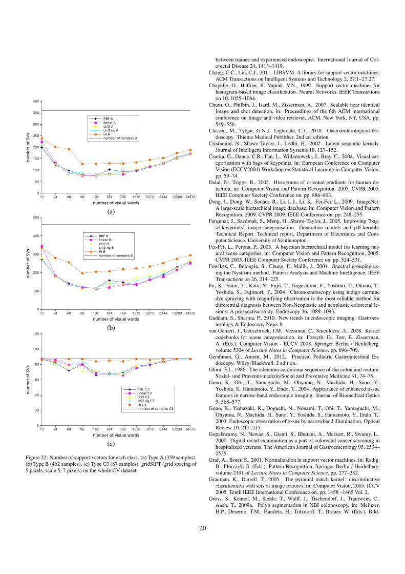
12 24 48 96 192 384 768 1536 3072 6144 12288 24576


0

50

100

150

200

250

300

350

400

num

ber

of

SV

s

RBF Alinear Achi2 Achi2 ng AHI Anumber of samples A

(a)

12 24 48 96 192 384 768 1536 3072 6144 12288 24576


0

100

200

300

400

500

num

ber

of

SV

s

RBF Blinear Bchi2 Bchi2 ng BHI Bnumber of samples B

(b)

12 24 48 96 192 384 768 1536 3072 6144 12288 24576


0

20

40

60

80

100

120

num

ber

of

SV

s

RBF C3linear C3chi2 C3chi2 ng C3HI C3number of samples C3

(c)

Figure 22: Number of support vectors for each class. (a) Type A (359 samples).(b) Type B (462 samples). (c) Type C3 (87 samples). gridSIFT (grid spacing of5 pixels, scale 5, 7 pixels) on the whole CV dataset.

between trainee and experienced endoscopist. International Journal of Col-orectal Disease 24, 1413–1419.

Chang, C.C., Lin, C.J., 2011. LIBSVM: A library for support vector machines.ACM Transactions on Intelligent Systems and Technology 2, 27:1–27:27.

Chapelle, O., Haffner, P., Vapnik, V.N., 1999. Support vector machines forhistogram-based image classification. Neural Networks, IEEE Transactionson 10, 1055–1064.

Chum, O., Philbin, J., Isard, M., Zisserman, A., 2007. Scalable near identicalimage and shot detection, in: Proceedings of the 6th ACM internationalconference on Image and video retrieval, ACM, New York, NY, USA. pp.549–556.

Classen, M., Tytgat, G.N.J., Lightdale, C.J., 2010. Gastroenterological En-doscopy. Thieme Medical Publither. 2nd ed. edition.

Cristianini, N., Shawe-Taylor, J., Lodhi, H., 2002. Latent semantic kernels.Journal of Intelligent Information Systems 18, 127–152.

Csurka, G., Dance, C.R., Fan, L., Willamowski, J., Bray, C., 2004. Visual cat-egorization with bags of keypoints, in: European Conference on ComputerVision (ECCV2004) Workshop on Statistical Learning in Computer Vision,pp. 59–74.

Dalal, N., Triggs, B., 2005. Histograms of oriented gradients for human de-tection, in: Computer Vision and Pattern Recognition, 2005. CVPR 2005.IEEE Computer Society Conference on, pp. 886–893.

Deng, J., Dong, W., Socher, R., Li, L.J., Li, K., Fei-Fei, L., 2009. ImageNet:A large-scale hierarchical image database, in: Computer Vision and PatternRecognition, 2009. CVPR 2009. IEEE Conference on, pp. 248–255.

Farquhar, J., Szedmak, S., Meng, H., Shawe-Taylor, J., 2005. Improving ”bag-of-keypoints” image categorisation: Generative models and pdf-kernels.Technical Report. Technical report, Department of Electronics and Com-puter Science, University of Southampton.

Fei-Fei, L., Perona, P., 2005. A bayesian hierarchical model for learning nat-ural scene categories, in: Computer Vision and Pattern Recognition, 2005.CVPR 2005. IEEE Computer Society Conference on, pp. 524–531.

Fowlkes, C., Belongie, S., Chung, F., Malik, J., 2004. Spectral grouping us-ing the Nystrom method. Pattern Analysis and Machine Intelligence, IEEETransactions on 26, 214–225.

Fu, K., Sano, Y., Kato, S., Fujii, T., Nagashima, F., Yoshino, T., Okuno, T.,Yoshida, S., Fujimori, T., 2004. Chromoendoscopy using indigo carminedye spraying with magnifying observation is the most reliable method fordifferential diagnosis between Non-Neoplastic and neoplastic colorectal le-sions: A prospective study. Endoscopy 36, 1089–1093.

Gaddam, S., Sharma, P., 2010. New trends in endoscopic imaging. Gastroen-terology & Endoscopy News 8.

van Gemert, J., Geusebroek, J.M., Veenman, C., Smeulders, A., 2008. Kernelcodebooks for scene categorization, in: Forsyth, D., Torr, P., Zisserman,A. (Eds.), Computer Vision - ECCV 2008. Springer Berlin / Heidelberg.volume 5304 of Lecture Notes in Computer Science, pp. 696–709.

Gershman, G., Ament, M., 2012. Practical Pediatric Gastrointestinal En-doscopy. Wiley-Blackwell. 2 edition.

Gloor, F.J., 1986. The adenoma-carcinoma sequence of the colon and rectum.Sozial- und Praventivmedizin/Social and Preventive Medicine 31, 74–75.

Gono, K., Obi, T., Yamaguchi, M., Ohyama, N., Machida, H., Sano, Y.,Yoshida, S., Hamamoto, Y., Endo, T., 2004. Appearance of enhanced tissuefeatures in narrow-band endoscopic imaging. Journal of Biomedical Optics9, 568–577.

Gono, K., Yamazaki, K., Doguchi, N., Nonami, T., Obi, T., Yamaguchi, M.,Ohyama, N., Machida, H., Sano, Y., Yoshida, S., Hamamoto, Y., Endo, T.,2003. Endoscopic observation of tissue by narrowband illumination. OpticalReview 10, 211–215.

Gopalswamy, N., Newaz, S., Gianti, S., Bhutani, A., Markert, R., Swamy, L.,2000. Digital rectal examination as a part of colorectal cancer screening inhospitalized veterans. The American Journal of Gastroenterology 95, 2534–2535.

Graf, A., Borer, S., 2001. Normalization in support vector machines, in: Radig,B., Florczyk, S. (Eds.), Pattern Recognition. Springer Berlin / Heidelberg.volume 2191 of Lecture Notes in Computer Science, pp. 277–282.

Grauman, K., Darrell, T., 2005. The pyramid match kernel: discriminativeclassification with sets of image features, in: Computer Vision, 2005. ICCV2005. Tenth IEEE International Conference on, pp. 1458 –1465 Vol. 2.

Gross, S., Kennel, M., Stehle, T., Wulff, J., Tischendorf, J., Trautwein, C.,Aach, T., 2009a. Polyp segmentation in NBI colonoscopy, in: Meinzer,H.P., Deserno, T.M., Handels, H., Tolxdorff, T., Brauer, W. (Eds.), Bild-

20

verarbeitung fur die Medizin 2009. Springer Berlin Heidelberg. Informatikaktuell, pp. 252–256.

Gross, S., Stehle, T., Behrens, A., Auer, R., Aach, T., Winograd, R., Trautwein,C., Tischendorf, J., 2009b. A comparison of blood vessel features and lo-cal binary patterns for colorectal polyp classification, in: Proc. of MedicalImaging 2008: Computer-Aided Diagnosis, SPIE. pp. 72602Q–72602Q–8.

Gunduz-Demir, C., Kandemir, M., Tosun, A.B., Sokmensuer, C., 2010. Au-tomatic segmentation of colon glands using object-graphs. Medical ImageAnalysis 14, 1–12.

Haasdonk, B., Bahlmann, C., 2004. Learning with distance substitution ker-nels, in: Rasmussen, C., Bulthoff, H., Scholkopf, B., Giese, M. (Eds.), Pat-tern Recognition – Proc. of the 26th DAGM Symposium. Springer Berlin /

Heidelberg. volume 3175 of Lecture Notes in Computer Science, pp. 220–227.

Hafner, M., Gangl, A., Kwitt, R., Uhl, A., Vecsei, A., Wrba, F., 2009a. Improv-ing pit-pattern classification of endoscopy images by a combination of ex-perts, in: Yang, G.Z., Hawkes, D., Rueckert, D., Noble, A., Taylor, C. (Eds.),Medical Image Computing and Computer-Assisted Intervention - MICCAI2009. Springer Berlin / Heidelberg. volume 5761 of Lecture Notes in Com-puter Science, pp. 247–254.

Hafner, M., Gangl, A., Liedlgruber, M., Uhl, A., Vecsei, A., Wrba, F., 2009b.Combining gaussian markov random fields with the discrete wavelet trans-form for endoscopic image classification, in: Proceedings of the 16th inter-national conference on Digital Signal Processing, IEEE Press, Piscataway,NJ, USA. pp. 177–182.

Hafner, M., Gangl, A., Liedlgruber, M., Uhl, A., Vecsei, A., Wrba, F., 2009c.Pit pattern classification using extended local binary patterns, in: Informa-tion Technology and Applications in Biomedicine, 2009. ITAB 2009. 9thInternational Conference on, pp. 1–4.

Hafner, M., Gangl, A., Liedlgruber, M., Uhl, A., Vecsei, A., Wrba, F., 2009d.Pit pattern classification using multichannel features and multiclassification,in: Exarchos, T., Papadopoulos, A., Fotiadis, D. (Eds.), Handbook of Re-search on Advanced Techniques in Diagnostic Imaging and Biomedical Ap-plications. IGI Global, Hershey, PA, USA, pp. 335–350.

Hafner, M., Gangl, A., Liedlgruber, M., Uhl, A., Vecsei, A., Wrba, F.,2010a. Classification of endoscopic images using delaunay triangulation-based edge features, in: Campilho, A., Kamel, M. (Eds.), Image Analy-sis and Recognition. Springer Berlin / Heidelberg. volume 6112 of LectureNotes in Computer Science, pp. 131–140.

Hafner, M., Gangl, A., Liedlgruber, M., Uhl, A., Vecsei, A., Wrba, F., 2010b.Endoscopic image classification using Edge-Based features, in: Proc. of20th International Conference on Pattern Recognition (ICPR2010), IEEE.pp. 2724–2727.

Hafner, M., Kendlbacher, C., Mann, W., Taferl, W., Wrba, F., Gangl, A., Vecsei,A., Uhl, A., 2006. Pit pattern classification of zoom-endoscopic colon im-ages using histogram techniques, in: Signal Processing Symposium, 2006.NORSIG 2006. Proceedings of the 7th Nordic, pp. 58–61.

Hafner, M., Kwitt, R., Uhl, A., Gangl, A., Wrba, F., Vecsei, A., 2009e. Featureextraction from multi-directional multi-resolution image transformations forthe classification of zoom-endoscopy images. Pattern Analysis & Applica-tions 12, 407–413.

Hafner, M., Kwitt, R., Uhl, A., Wrba, F., Gangl, A., Vecsei, A., 2009f.Computer-assisted pit-pattern classification in different wavelet domains forsupporting dignity assessment of colonic polyps. Pattern Recognition 42,1180–1191.

Hafner, M., Kwitt, R., Wrba, F., Gangl, A., Vecsei, A., Uhl, A., 2008. One-against-one classification for zoom-endoscopy images, in: Advances inMedical, Signal and Information Processing, 2008. MEDSIP 2008. 4th IETInternational Conference on, pp. 1–4.

Halligan, S., Taylor, S.A., 2007. CT colonography: Results and limitations.European Journal of Radiology 61, 400–408.

Harris, C., Stephens, M., 1988. A combined corner and edge detector, in: Proc.of 4th Alvey Vision Conference (AVC1988), pp. 147–151.

Hastie, T., 2009. The elements of statistical learning : data mining, inference,and prediction. Springer, New York. 2nd ed. edition.

Health statistics and informatics Department, World Health Organization,2008. Global Burden of Disease: 2004 update. http://www.who.int/

evidence/bod.Heitman, S.J., Au, F., Manns, B.J., McGregor, S.E., Hilsden, R.J., 2008. Non-

medical costs of colorectal cancer screening with the fecal occult blood testand colonoscopy. Clinical Gastroenterology and Hepatology 6, 912 – 917.

Herve, N., Boujemaa, N., Houle, M.E., 2009. Document description: whatworks for images should also work for text?, in: Multimedia Content Ac-cess: Algorithms and Systems III, SPIE. pp. 72550B–72550B–12.

Higashi, R., Uraoka, T., Kato, J., Kuwaki, K., Ishikawa, S., Saito, Y., Mat-suda, T., Ikematsu, H., Sano, Y., Suzuki, S., Murakami, Y., Yamamoto, K.,2010. Diagnostic accuracy of narrow-band imaging and pit pattern analysissignificantly improved for less-experienced endoscopists after an expandedtraining program. Gastrointestinal Endoscopy 72, 127–135.

Hirai, K., Kanazawa, Y., Sagawa, R., Yagi, Y., 2011. Endoscopic image match-ing for reconstructing the 3-D structure of the intestines. Medical ImagingTechnology 29, 36–46.

Hirata, M., Tanaka, S., Oka, S., Kaneko, I., Yoshida, S., Yoshihara, M.,Chayama, K., 2007a. Evaluation of microvessels in colorectal tumors bynarrow band imaging magnification. Gastrointestinal Endoscopy 66, 945–952.

Hirata, M., Tanaka, S., Oka, S., Kaneko, I., Yoshida, S., Yoshihara, M.,Chayama, K., 2007b. Magnifying endoscopy with narrow band imaging fordiagnosis of colorectal tumors. Gastrointestinal Endoscopy 65, 988–995.

Hofmann, T., 1999. Probabilistic latent semantic analysis, in: 15th Uncertaintyin Artificial Intelligence, pp. 289–296.

Hsu, C.W., Chang, C.C., , Lin, C.J., 2003. A practical guide to supportvector classification. http://www.csie.ntu.edu.tw/~cjlin/papers/guide/guide.pdf.

Hsu, C.W., Lin, C.J., 2002. A comparison of methods for multiclass supportvector machines. Neural Networks, IEEE Transactions on 13, 415–425.

Huang, T.K., Weng, R.C., Lin, C.J., 2006. Generalized bradley-terry mod-els and multi-class probability estimates. Journal of Machine Learning Re-search 4.

Ignjatovic, A., East, J.E., Guenther, T., Hoare, J., Morris, J., Ragunath, K.,Shonde, A., Simmons, J., Suzuki, N., Thomas-Gibson, S., Saunders, B.,2011. What is the most reliable imaging modality for small colonic polypcharacterization? Study of white-light, autofluorescence, and narrow-bandimaging. Endoscopy 43, 94–99.

Ikematsu, H., Matsuda, T., Emura, F., Saito, Y., Uraoka, T., Fu, K.I., Kaneko,K., Ochiai, A., Fujimori, T., Sano, Y., 2010. Efficacy of capillary patterntype IIIA/IIIB by magnifying narrow band imaging for estimating depth ofinvasion of early colorectal neoplasms. BMC Gastroenterology 10, 33.

Imai, Y., Kudo, S., Tsuruta, O., Fujii, T., Hayashi, S., Tanaka, S., Terai, T.,2001. Problems and clinical significance of v type pit pattern diagnosis:report on round-table consensus meeting. Early Colorectal Cancer 5, 595–613.

Jenkinson, F., Steele, R., 2010. Colorectal cancer screening – methodology.The Surgeon 8, 164 – 171.

Joachims, T., 1998. Text categorization with support vector machines: Learningwith many relevant features, in: Nedellec, C., Rouveirol, C. (Eds.), MachineLearning: ECML-98. Springer Berlin / Heidelberg. volume 1398 of LectureNotes in Computer Science, pp. 137–142.

John C. Platt, Nello Cristianini, J.S.T., 2000. Large margin dags for multiclassclassification, in: Advances in Neural Information Processing Systems 12(NIPS1999), pp. 547–553.

John Shawe-Taylor, N.C., 2000. An introduction to support vector machines: and other kernel-based learning methods. Cambridge University Press,Cambridge; New York.

Johnson, C., MacCarty, R.L., Welch, T.J., Wilson, L.A., Harmsen, W.S., Il-strup, D.M., Ahlquist, D.A., 2004. Comparison of the relative sensitivity ofct colonography and double-contrast barium enema for screen detection ofcolorectal polyps. Clinical Gastroenterology and Hepatology 2, 314–321.

Joutou, T., Yanai, K., 2009. A food image recognition system with multiplekernel learning, in: Image Processing (ICIP), 2009 16th IEEE InternationalConference on, pp. 285–288.

Jurie, F., Triggs, B., 2005. Creating efficient codebooks for visual recognition,in: Computer Vision, 2005. ICCV 2005. Tenth IEEE International Confer-ence on, pp. 604–610.

Kanao, H., 2008. Clinical significance of type VI pit pattern subclassificationin determining the depth of invasion of colorectal neoplasms. World Journalof Gastroenterology 14, 211–217.

Kanao, H., Tanaka, S., Oka, S., Hirata, M., Yoshida, S., Chayama, K., 2009.Narrow-band imaging magnification predicts the histology and invasiondepth of colorectal tumors. Gastrointestinal Endoscopy 69, 631–636.

Karkanis, S., Iakovidis, D., Maroulis, D., Karras, D., Tzivras, M., 2003.Computer-aided tumor detection in endoscopic video using color wavelet

21

features. Information Technology in Biomedicine, IEEE Transactions on 7,141–152.

Karl, J., Wild, N., Tacke, M., Andres, H., Garczarek, U., Rollinger, W., Zolg,W., 2008. Improved diagnosis of colorectal cancer using a combination offecal occult blood and novel fecal protein markers. Clinical Gastroenterol-ogy and Hepatology 6, 1122–1128.

Ke, Y., Sukthankar, R., 2004. PCA-SIFT: a more distinctive representation forlocal image descriptors, in: Computer Vision and Pattern Recognition, 2004.CVPR 2004. Proceedings of the 2004 IEEE Computer Society Conferenceon, pp. II–506–II–513.

Kiesslich, R., Goetz, M., Vieth, M., Galle, P.R., Neurath, M.F., 2007. Tech-nology insight: confocal laser endoscopy for in vivo diagnosis of colorectalcancer. Nature Reviews Clinical Oncology 4, 480–490.

Koenderink, J., 1984. The structure of images. Biological Cybernetics 50,363–370.

Kosaka, T., 1975. Fundamental study on the diminutive polyps of the colonby mucosal stain and dissecting microscope. Journal of Coloproctology 28,218–228.

Kudo, S., Hirota, S., Nakajima, T., Hosobe, S., Kusaka, H., Kobayashi, T.,Himori, M., Yagyuu, A., 1994. Colorectal tumours and pit pattern. Journalof Clinical Pathology 47, 880–885.

Kudo, S., Tamura, S., Nakajima, T., Yamano, H., Kusaka, H., Watanabe, H.,1996. Diagnosis of colorectal tumorous lesions by magnifying endoscopy.Gastrointestinal Endoscopy 44, 8–14.

Kwitt, R., Uhl, A., 2007a. Modeling the marginal distributions of complexwavelet coefficient magnitudes for the classification of Zoom-Endoscopyimages, in: Proc. of ICCV2007, IEEE. pp. 1–8.

Kwitt, R., Uhl, A., 2007b. Multi-directional multi-resolution transforms forzoom-endoscopy image classification, in: Kurzynski, M., Puchala, E., Woz-niak, M., Zolnierek, A. (Eds.), Computer Recognition Systems 2. SpringerBerlin / Heidelberg. volume 45 of Advances in Soft Computing, pp. 35–43.

Kwitt, R., Uhl, A., 2008. Color eigen-subband features for endoscopy imageclassification, in: Acoustics, Speech and Signal Processing, 2008. ICASSP2008. IEEE International Conference on, pp. 589– –592.

Kwitt, R., Uhl, A., Hafner, M., Gangl, A., Wrba, F., Vecsei, A., 2010. Predict-ing the histology of colorectal lesions in a probabilistic framework, in: Proc.of CVPR2010 Workshop on Mathematical Methods in Biomedical ImageAnalysis (MMBIA2010), IEEE. pp. 103–110.

Lazebnik, S., Schmid, C., Ponce, J., 2006. Beyond bags of features: Spatialpyramid matching for recognizing natural scene categories, in: ComputerVision and Pattern Recognition, 2006 IEEE Computer Society Conferenceon, pp. 2169–2178.

Lee, Y., Lin, Y., Wahba, G., 2001. Multicategory Support Vector Machines.Technical Report. Department of Statistics, University of Madison.

Lin, M., Wong, K., Ng, W.L., Shon, I.H., Morgan, M., 2011. Positronemission tomography and colorectal cancer. Critical Reviews in Oncol-ogy/Hematology 77, 30–47.

Lindeberg, T., 1994. Scale-space theory: a basic tool for analyzing structuresat different scales. Journal of Applied Statistics 21, 225–270.

Lodhi, H., Saunders, C., Shawe-Taylor, J., Cristianini, N., Watkins, C., 2002.Text classification using string kernels. J. Mach. Learn. Res. 2, 419–444.

Lowe, D.G., 1999. Object recognition from local scale-invariant features. Com-puter Vision, IEEE International Conference on 2, 1150.

Lowe, D.G., 2004. Distinctive image features from scale-invariant keypoints.International Journal of Computer Vision 60, 91–110.

Machida, H., Sano, Y., Hamamoto, Y., Muto, M., Kozu, T., Tajiri, H., Yoshida,S., 2004. Narrow-Band imaging in the diagnosis of colorectal mucosal le-sions: A pilot study. Endoscopy 36, 1094–1098.

Maji, S., Berg, A., Malik, J., 2008. Classification using intersection kernel sup-port vector machines is efficient, in: Computer Vision and Pattern Recogni-tion, 2008. CVPR 2008. IEEE Conference on, pp. 1–8.

Maroulis, D., Iakovidis, D., Karkanis, S., Karras, D., 2003. CoLD: a versatiledetection system for colorectal lesions in endoscopy video-frames. Com-puter Methods and Programs in Biomedicine 70, 151 – 166.

Matsumoto, A., Tanaka, S., Oba, S., Kanao, H., Oka, S., Yoshihara, M.,Chayama, K., 2010. Outcome of endoscopic submucosal dissection forcolorectal tumors accompanied by fibrosis. Scandinavian Journal of Gas-troenterology 45, 1329–1337.

Matsushima, C., Yamauchi, Y., Yamashita, T., Fujiyoshi, H., 2010. Object de-tection using relational binarized HOG feature and binary selection by realadaboost, in: Proc. of the 13th Meeting on Image Recognition and Under-

standing (MIRU2010), pp. 18–25.Mayinger, B., Oezturk, Y., Stolte, M., Faller, G., Benninger, J., Schwab, D.,

Maiss, J., Hahn, E.G., Muehldorfer, S., 2006. Evaluation of sensitivity andinter- and intra-observer variability in the detection of intestinal metapla-sia and dysplasia in barrett’s esophagus with enhanced magnification en-doscopy. Scandinavian Journal of Gastroenterology 41, 349–356.

Meining, A., Rosch, T., Kiesslich, R., Muders, M., Sax, F., Heldwein, W., 2004.Inter- and Intra-Observer Variability of Magnification Chromoendoscopy forDetecting Specialized Intestinal Metaplasia at the Gastroesophageal Junc-tion. Endoscopy 36, 160–164.

Mikolajczyk, K., Schmid, C., 2003. A performance evaluation of local descrip-tors, in: Computer Vision and Pattern Recognition, 2003. Proceedings. 2003IEEE Computer Society Conference on, pp. II–257–II–263.

Mikolajczyk, K., Schmid, C., 2004. Scale & affine invariant interest point de-tectors. International Journal of Computer Vision 60, 63–86.

Mikolajczyk, K., Schmid, C., 2005. A performance evaluation of local descrip-tors. Pattern Analysis and Machine Intelligence, IEEE Transactions on 27,1615–1630.

Milgram, J., Cheriet, M., Sabourin, R., 2006. One against one or one againstall: Which one is better for handwriting recognition with SVMs?, in: Proc.of 10th International Workshop on Frontiers in Handwriting Recognition.

Ministry of Health, Labour and Welfare, Japan, 2009. Vital Statistics in Japan— The latest trends —. http://www.mhlw.go.jp/english/database/db-hw/vs01.html.

Muller, H., Kalpathy-Cramer, J., Kahn, C., Hatt, W., Bedrick, S., Hersh, W.,2009. Overview of the ImageCLEFmed 2008 medical image retrieval task,in: Peters, C., Deselaers, T., Ferro, N., Gonzalo, J., Jones, G., Kurimo, M.,Mandl, T., Penas, A., Petras, V. (Eds.), Evaluating Systems for Multilingualand Multimodal Information Access. Springer Berlin / Heidelberg. volume5706 of Lecture Notes in Computer Science, pp. 512–522.

Muller, H., Michoux, N., Bandon, D., Geissbuhler, A., 2004. A review ofcontent-based image retrieval systems in medical applications – clinical ben-efits and future directions. International Journal of Medical Informatics 73,1–23.

Nakayama, H., Harada, T., Kuniyoshi, Y., 2010. Global gaussian approach forscene categorization using information geometry, in: Computer Vision andPattern Recognition (CVPR), 2010 IEEE Conference on, pp. 2336–2343.

National Cancer Institute, US National Institutes of Health, 2010. Colonand Rectal Cancer. http://www.cancer.gov/cancertopics/types/

colon-and-rectal.Nister, D., Stewenius, H., 2006. Scalable recognition with a vocabulary tree,

in: Computer Vision and Pattern Recognition, 2006 IEEE Computer SocietyConference on, pp. 2161–2168.

Nowak, E., Jurie, F., Triggs, B., 2006. Sampling strategies for bag-of-featuresimage classification, in: Leonardis, A., Bischof, H., Pinz, A. (Eds.), Com-puter Vision - ECCV 2006. Springer Berlin / Heidelberg. volume 3954 ofLecture Notes in Computer Science, pp. 490–503.

Oba, S., Tanaka, S., Oka, S., Kanao, H., Yoshida, S., Shimamoto, F., Chayama,K., 2010. Characterization of colorectal tumors using narrow-band imagingmagnification: combined diagnosis with both pit pattern and microvesselfeatures. Scandinavian Journal of Gastroenterology 45, 1084–1092.

Oba, S., Tanaka, S., Sano, Y., Oka, S., Chayama, K., 2011. Current status ofNarrow-Band imaging magnifying colonoscopy for colorectal neoplasia injapan. Digestion 83, 167–172.

Oh, J., Hwang, S., Lee, J., Tavanapong, W., Wong, J., de Groen, P.C., 2007. In-formative frame classification for endoscopy video. Medical Image Analysis11, 110–127.

Onji, K., Yoshida, S., Tanaka, S., Kawase, R., Takemura, Y., Oka, S., Tamaki,T., Raytchev, B., Kaneda, K., Yoshihara, M., Chayama, K., 2011. Quantita-tive analysis of colorectal lesions observed on magnified endoscopy images.Journal of Gastroenterology 46, 1382–1390. 10.1007/s00535-011-0459-x.

Oto, A., 2002. Virtual endoscopy. European Journal of Radiology 42, 231–239.Padhani, A.R., 1999. Advances in imaging of colorectal cancer. Critical Re-

views in Oncology/Hematology 30, 189–199.Panossian, A.M., Raimondo, M., Wolfsen, H.C., 2011. State of the art in the

endoscopic imaging and ablation of barrett’s esophagus. Digestive and LiverDisease 43, 365–373.

Perronnin, F., 2008. Universal and adapted vocabularies for generic visual cat-egorization. Pattern Analysis and Machine Intelligence, IEEE Transactionson 30, 1243–1256.

Perronnin, F., Dance, C., Csurka, G., Bressan, M., 2006. Adapted vocabularies

22

for generic visual categorization, in: Leonardis, A., Bischof, H., Pinz, A.(Eds.), Computer Vision - ECCV 2006. Springer Berlin / Heidelberg. vol-ume 3954 of Lecture Notes in Computer Science, pp. 464–475.

Philbin, J., Chum, O., Isard, M., Sivic, J., Zisserman, A., 2007. Object retrievalwith large vocabularies and fast spatial matching, in: Computer Vision andPattern Recognition, 2007. CVPR ’07. IEEE Conference on, pp. 1–8.

Philbin, J., Chum, O., Isard, M., Sivic, J., Zisserman, A., 2008. Lost in quanti-zation: Improving particular object retrieval in large scale image databases,in: Computer Vision and Pattern Recognition, 2008. CVPR 2008. IEEEConference on, pp. 1–8.

Qiu, B., Yanai, K., 2008. Objects over the world, in: Huang, Y.M., Xu, C.,Cheng, K.S., Yang, J.F., Swamy, M., Li, S., Ding, J.W. (Eds.), Advances inMultimedia Information Processing - PCM 2008. Springer Berlin / Heidel-berg. volume 5353 of Lecture Notes in Computer Science, pp. 296–305.

Quelhas, P., Odobez, J.M., 2007. Multi-level local descriptor quantization forbag-of-visterms image representation, in: Proceedings of the 6th ACM in-ternational conference on Image and video retrieval, ACM, New York, NY,USA. pp. 242–249.

Raghavendra, M., Hewett, D.G., Rex, D.K., 2010. Differentiating adenomasfrom hyperplastic colorectal polyps: narrow-band imaging can be learned in20 minutes. Gastrointestinal Endoscopy 72, 572–576.

Rex, D.K., Kahi, C., O’Brien, M., Levin, T., Pohl, H., Rastogi, A., Burgart, L.,Imperiale, T., Ladabaum, U., Cohen, J., 2011. The american society for gas-trointestinal endoscopy PIVI (Preservation and incorporation of valuable en-doscopic innovations) on real-time endoscopic assessment of the histologyof diminutive colorectal polyps. Gastrointestinal Endoscopy 73, 419–422.

Saito, S., Tajiri, H., Ohya, T., Nikami, T., Aihara, H., Ikegami, M., 2011. Imag-ing by magnifying endoscopy with NBI implicates the remnant capillarynetwork as an indication for endoscopic resection in early colon cancer. In-ternational Journal of Surgical Oncology 2011, 1–10.

Saito, Y., Uraoka, T., Matsuda, T., Emura, F., Ikehara, H., Mashimo, Y.,Kikuchi, T., Fu, K.I., Sano, Y., Saito, D., 2007. Endoscopic treatment oflarge superficial colorectal tumors: a case series of 200 endoscopic submu-cosal dissections (with video). Gastrointestinal Endoscopy 66, 966–973.

Sanford, K.W., McPherson, R.A., 2009. Fecal occult blood testing. Clinics inLaboratory Medicine 29, 523–541.

Sano, Y., Horimatsu, T., Fu, K.I., Katagiri, A., Muto, M., Ishikawa, H., 2006.Magnifying observation of microvascular architecture of colorectal lesionsusing a narrow-band imaging system. Digestive Endoscopy 18, S44–S51.

Sano, Y., Ikematsu, H., Fu, K.I., Emura, F., Katagiri, A., Horimatsu, T.,Kaneko, K., Soetikno, R., Yoshida, S., 2009. Meshed capillary vessels byuse of narrow-band imaging for differential diagnosis of small colorectalpolyps. Gastrointestinal Endoscopy 69, 278–283.

Schmid, C., Mohr, R., 1997. Local grayvalue invariants for image retrieval.Pattern Analysis and Machine Intelligence, IEEE Transactions on 19, 530–535.

Scholkopf, B., Smola, A.J., 2002. Learning with kernels : support vector ma-chines, regularization, optimization, and beyond. MIT Press, CambridgeMass. [u.a.].

Shin, L.K., Poullos, P., Jeffrey, R.B., 2010. MR colonography and MR enterog-raphy. Gastrointestinal Endoscopy Clinics of North America 20, 323–346.

Shotton, J., Johnson, M., Cipolla, R., 2008. Semantic texton forests for imagecategorization and segmentation, in: Computer Vision and Pattern Recogni-tion, 2008. CVPR 2008. IEEE Conference on, pp. 1–8.

Sivic, J., Zisserman, A., 2003. Video Google: a text retrieval approach toobject matching in videos, in: Computer Vision, 2003. Proceedings. NinthIEEE International Conference on, pp. 1470–1477.

Sonnenburg, S., Ratsch, G., Schafer, C., Scholkopf, B., 2006. Large scalemultiple kernel learning. Journal of Machine Learning Research , 1531–1565.

Stehle, T., Auer, R., Gross, S., Behrens, A., Wulff, J., Aach, T., Winograd,R., Trautwein, C., Tischendorf, J., 2009. Classification of colon polyps inNBI endoscopy using vascularization features, in: Proc. of Medical Imaging2009: Computer-Aided Diagnosis, SPIE. pp. 72602S–72602S–12.

Steinwart, I., Christmann, A., 2008. Support vector machines. Springer, NewYork. 1st ed. edition.

Sundaram, P., Zomorodian, A., Beaulieu, C., Napel, S., 2008. Colon polypdetection using smoothed shape operators: Preliminary results. MedicalImage Analysis 12, 99–119.

Swain, M.J., Ballard, D.H., 1991. Color indexing. International Journal ofComputer Vision 7, 11–32. 10.1007/BF00130487.

Takemura, Y., Yoshida, S., Tanaka, S., Kawase, R., Onji, K., Oka, S., Tamaki,T., Raytchev, B., Kaneda, K., Yoshihara, M., Chayama, K., 2012. Computer-aided system for predicting the histology of colorectal tumors by usingnarrow-band imaging magnifying colonoscopy (with video). Gastrointesti-nal Endoscopy 75, 179–185.

Takemura, Y., Yoshida, S., Tanaka, S., Onji, K., Oka, S., Tamaki, T., Kaneda,K., Yoshihara, M., Chayama, K., 2010. Quantitative analysis and develop-ment of a computer-aided system for identification of regular pit patterns ofcolorectal lesions. Gastrointestinal Endoscopy 72, 1047 – 1051.

Tamai, N., Sakamoto, T., Nakajima, T., Matsuda, T., Saito, Y., Tajiri, H.,Koyama, R., Kido, S., 2011. Su1566 computer-assisted automatic iden-tification system for colorectal narrow band imaging (NBI) classification.Gastrointestinal Endoscopy 73, AB306–AB307.

Tamaki, T., Yoshimuta, J., Takeda, T., Raytchev, B., Kaneda, K., Yoshida, S.,Takemura, Y., Tanaka, S., 2011. A system for colorectal tumor classifi-cation in magnifying endoscopic NBI images, in: Kimmel, R., Klette, R.,Sugimoto, A. (Eds.), Computer Vision - ACCV 2010. Springer Berlin / Hei-delberg. volume 6493 of Lecture Notes in Computer Science, pp. 452–463.

Tamegai, Y., 2007. Endoscopic submucosal dissection (ESD) for large col-orectal tumors comparing with endoscopic piecemeal mucosal resection(EPMR). Gastrointestinal Endoscopy 65, AB275.

Tanaka, S., Kaltenbach, T., Chayama, K., Soetikno, R., 2006. High-magnification colonoscopy (with videos). Gastrointestinal Endoscopy 64,604–613.

Tischendorf, J., Gross, S., Winograd, R., Hecker, H., Auer, R., Behrens, A.,Trautwein, C., Aach, T., Stehle, T., 2010. Computer-aided classification ofcolorectal polyps based on vascular patterns: a pilot study. Endoscopy 42,203–207.

Tong, S., Koller, D., 2002. Support vector machine active learning with appli-cations to text classification. J. Mach. Learn. Res. 2, 45–66.

Tosun, A.B., Kandemir, M., Sokmensuer, C., Gunduz-Demir, C., 2009. Object-oriented texture analysis for the unsupervised segmentation of biopsy im-ages for cancer detection. Pattern Recognition 42, 1104–1112.

Tuytelaars, T., 2010. Dense interest points. Computer Vision and PatternRecognition, IEEE Computer Society Conference on 0, 2281–2288.

Tuytelaars, T., Mikolajczyk, K., 2007. Local invariant feature detectors: Asurvey. Foundations and Trends R© in Computer Graphics and Vision 3, 177–280.

Tweedle, E., Rooney, P., Watson, A., 2007. Screening for rectal cancer? will itimprove cure rates? Clinical Oncology 19, 639–648.

Vapnik, V.N., 1998. Statistical learning theory. Wiley, New York [u.a.].Vedaldi, A., Fulkerson, B., 2008. VLFeat: An open and portable library of

computer vision algorithms. http://www.vlfeat.org/.Vedaldi, A., Zisserman, A., 2012. Efficient additive kernels via explicit feature

maps. Pattern Analysis and Machine Intelligence, IEEE Transactions on 34,480–492.

Wada, Y., Kudo, S., Kashida, H., Ikehara, N., Inoue, H., Yamamura, F., Oht-suka, K., Hamatani, S., 2009. Diagnosis of colorectal lesions with the mag-nifying narrow-band imaging system. Gastrointestinal Endoscopy 70, 522–531.

Watanabe, T., Itabashi, M., Shimada, Y., Tanaka, S., Ito, Y., Ajioka, Y., Ham-aguchi, T., Hyodo, I., Igarashi, M., Ishida, H., Ishiguro, M., Kanemitsu, Y.,Kokudo, N., Muro, K., Ochiai, A., Oguchi, M., Ohkura, Y., Saito, Y., Sakai,Y., Ueno, H., Yoshino, T., Fujimori, T., Koinuma, N., Morita, T., Nishimura,G., Sakata, Y., Takahashi, K., Takiuchi, H., Tsuruta, O., Yamaguchi, T.,Yoshida, M., Yamaguchi, N., Kotake, K., Sugihara, K., for Cancer of theColon, J.S., Rectum, 2012. Japanese Society for Cancer of the Colon andRectum (JSCCR) guidelines 2010 for the treatment of colorectal cancer. In-ternational Journal of Clinical Oncology 17, 1–29. 10.1007/s10147-011-0315-2.

Weston, J., Watkins, C., 1999. Support vector machines for multi-class pat-tern recognition, in: Proc. of 7th European Symposium on Artifical NeuralNetworks (ESANN1999), pp. 219–224.

Winn, J., Criminisi, A., Minka, T., 2005. Object categorization by learneduniversal visual dictionary, in: Computer Vision, 2005. ICCV 2005. TenthIEEE International Conference on, pp. 1800–1807.

Wu, C., . SiftGPU: A GPU implementation of scale invariant feature transform(SIFT). http://cs.unc.edu/~ccwu/siftgpu/.

Yanai, K., Qiu, B., 2009. Mining cultural differences from a large number ofgeotagged photos, in: Proceedings of the 18th international conference onWorld wide web, ACM, New York, NY, USA. pp. 1173–1174.

23

Ye, B.D., Byeon, J.S., Kwon, S., Kim, B., Myung, S.J., Yang, S.K., Kim, J.H.,2008. Clinical course of submucosal colorectal cancers treated by endo-scopic mucosal resection. Gastrointestinal Endoscopy 67, AB312.

Yoshida, H., Dachman, A.H., 2004. Computer-aided diagnosis for CT colonog-raphy. Seminars in Ultrasound, CT, and MRI 25, 419–431.

Zhang, J., Marszałek, M., Lazebnik, S., Schmid, C., 2007. Local features andkernels for classification of texture and object categories: A comprehensivestudy. International Journal of Computer Vision 73, 213–238.

Zhou, X., Zhuang, X., Yan, S., Chang, S.F., Hasegawa-Johnson, M., Huang,T.S., 2008. SIFT-Bag kernel for video event analysis, in: Proceeding of the16th ACM international conference on Multimedia, ACM, New York, NY,USA. pp. 229–238.

24

Computer-Aided Colorectal Tumor Classification in NBI Endoscopy Using Local Features

Documents

Transcript of Computer-Aided Colorectal Tumor Classification in NBI Endoscopy Using Local Features