Computational modeling of flow-induced anisotropy of polar ice for the EDML deep drilling site,...

INTERNATIONAL JOURNAL FOR NUMERICAL AND ANALYTICAL METHODS IN GEOMECHANICSInt. J. Numer. Anal. Meth. Geomech. (2011)Published online in Wiley Online Library (wileyonlinelibrary.com). DOI: 10.1002/nag.1034

Computational modeling of flow-induced anisotropy of polar icefor the EDML deep drilling site, Antarctica: The effect of rotation

recrystallization and grain boundary migration

Swantje Bargmann1,∗,†, Hakime Seddik2 and Ralf Greve2

1Institute of Mechanics, TU Dortmund, Germany2Institute of Low Temperature Science, Hokkaido University, Sapporo, Japan

SUMMARY

In this contribution we model flow-induced anisotropy of polar ice in order to gain a better understandingfor the underlying microstructure and its influence on the deformation process. In particular, a continuum-mechanical, anisotropic flow model that is based on an anisotropic flow enhancement factor (CAFFEmodel) is applied. The polycrystalline ice is regarded as a mixture whose grains are characterized bytheir orientation. The approach is based on two distinct scales: the underlying microstructure influencesthe macroscopic material behavior and is taken into account phenomenologically. To achieve this, theorientation mass density is introduced as a mesoscopic field, i.e. it depends on a mesoscopic variable (theorientation) in addition to position and time. The classical flow law of Glen is extended by a scalar, butanisotropic enhancement factor. Four different effects (local rigid body rotation, grain rotation, rotationrecrystallization, grain boundary migration) influencing the evolution of the grain orientations are takeninto account. All modeling parameters are either measurable in or derivable from field observations orlaboratory experiments. A finite volume method is chosen for the discretization procedure. Numericalresults simulating the ice flow at the site of the EPICA ice core in Dronning Maud Land (referred toas EDML), Antarctica, are presented. They go beyond earlier results by Seddik et al. (J. Glaciol. 2008;54(187):631–642) in which only local rigid body rotation and grain rotation were accounted for. Bycomparing simulated and observed fabrics, we come up with reference values for the parameters in theconstitutive equations for rotation recrystallization and grain boundary migration. Down to 2045 m depth,good agreement can be achieved; however, further down the observed fabric cannot be reproduced welldue to numerical issues. Additionally, we study the influence of the two superposed deformation regimesof vertical compression and simple shear separately and demonstrate that the numerical problems aredue to the predominant shear regime near the bottom, whereas vertical compression only produces stableresults everywhere. Copyright � 2011 John Wiley & Sons, Ltd.

Received 7 February 2011; Accepted 7 February 2011

KEY WORDS: anisotropy; fabric; orientation; EDML core; Antarctica; polar ice; computational modeling;continuum mechanics

1. INTRODUCTION

About 98% of the Earth’s southernmost continent Antarctica are covered by ice with an averageice thickness of approximately 2 km. With this, it stores about 70% of the world’s fresh water, andit is by far the largest single land ice body at present. In addition, the ice contains an abundanceof historic climate information. Researchers hope to obtain full documentation of the climatic and

∗Correspondence to: Swantje Bargmann, Institute of Mechanics, TU Dortmund, Leonhard-Euler-Str. 5, 44227Dortmund, Germany.

†E-mail: [email protected]

Copyright � 2011 John Wiley & Sons, Ltd.

S. BARGMANN, H. SEDDIK AND R. GREVE

(a) (b)

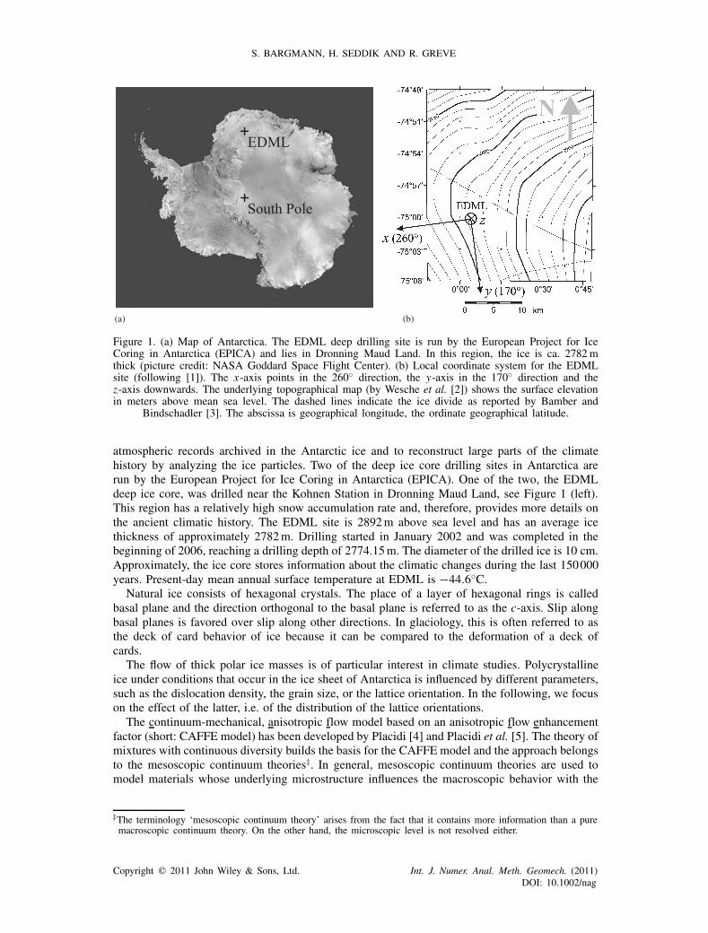
Figure 1. (a) Map of Antarctica. The EDML deep drilling site is run by the European Project for IceCoring in Antarctica (EPICA) and lies in Dronning Maud Land. In this region, the ice is ca. 2782mthick (picture credit: NASA Goddard Space Flight Center). (b) Local coordinate system for the EDMLsite (following [1]). The x-axis points in the 260◦ direction, the y-axis in the 170◦ direction and thez-axis downwards. The underlying topographical map (by Wesche et al. [2]) shows the surface elevationin meters above mean sea level. The dashed lines indicate the ice divide as reported by Bamber and

Bindschadler [3]. The abscissa is geographical longitude, the ordinate geographical latitude.

atmospheric records archived in the Antarctic ice and to reconstruct large parts of the climatehistory by analyzing the ice particles. Two of the deep ice core drilling sites in Antarctica arerun by the European Project for Ice Coring in Antarctica (EPICA). One of the two, the EDMLdeep ice core, was drilled near the Kohnen Station in Dronning Maud Land, see Figure 1 (left).This region has a relatively high snow accumulation rate and, therefore, provides more details onthe ancient climatic history. The EDML site is 2892m above sea level and has an average icethickness of approximately 2782m. Drilling started in January 2002 and was completed in thebeginning of 2006, reaching a drilling depth of 2774.15m. The diameter of the drilled ice is 10 cm.Approximately, the ice core stores information about the climatic changes during the last 150000years. Present-day mean annual surface temperature at EDML is −44.6◦C.

Natural ice consists of hexagonal crystals. The place of a layer of hexagonal rings is calledbasal plane and the direction orthogonal to the basal plane is referred to as the c-axis. Slip alongbasal planes is favored over slip along other directions. In glaciology, this is often referred to asthe deck of card behavior of ice because it can be compared to the deformation of a deck ofcards.

The flow of thick polar ice masses is of particular interest in climate studies. Polycrystallineice under conditions that occur in the ice sheet of Antarctica is influenced by different parameters,such as the dislocation density, the grain size, or the lattice orientation. In the following, we focuson the effect of the latter, i.e. of the distribution of the lattice orientations.

The continuum-mechanical, anisotropic flow model based on an anisotropic flow enhancementfactor (short: CAFFE model) has been developed by Placidi [4] and Placidi et al. [5]. The theory ofmixtures with continuous diversity builds the basis for the CAFFE model and the approach belongsto the mesoscopic continuum theories‡. In general, mesoscopic continuum theories are used tomodel materials whose underlying microstructure influences the macroscopic behavior with the

‡The terminology ‘mesoscopic continuum theory’ arises from the fact that it contains more information than a puremacroscopic continuum theory. On the other hand, the microscopic level is not resolved either.

Copyright � 2011 John Wiley & Sons, Ltd. Int. J. Numer. Anal. Meth. Geomech. (2011)DOI: 10.1002/nag

COMPUTATIONAL MODELING OF FLOW-INDUCED ANISOTROPY OF POLAR ICE

aid of a continuum theory. In addition to the general macroscopic field quantities which dependon position and time, a mesoscopic field is introduced which depends on a mesoscopic variable.The latter is governed by a mesoscopic balance equation. Some of the macroscopic quantities arethen defined in terms of the mesoscopic fields. This is a clear advantage in comparison to ordinarycontinuum mechanical theories as the additional information from the mesoscopic level is not lost.However, the underlying mesostructure is only modeled phenomenologically, thus, the mesoscopicequations do not govern the evolution of the crystallites. Rather, it is hidden in the theory and takeninto account indirectly. Moreover, the CAFFE model has a thermodynamic setting: it is postulatedin accordance to all material modeling principles, such as objectivity and determinism, and fulfillsthe second law of thermodynamics.

The CAFFE model has been set up for the case of large polar ice masses in which inducedanisotropy occurs. The grain size (and with it the number of grains per cross section) respectivelythe positions of the grains are not explicitly part of the theory. Rather, the grain orientations aremodeled as a continuous distribution. The anisotropy is governed by the evolution of the latticeorientation distribution of the ice crystallites. The distribution of grain orientations (fabric) isdescribed by the orientation mass balance and influenced by four distinct recrystallization effects:local rigid body rotation (i), grain rotation (ii), rotation recrystallization (iii), and grain boundarymigration (iv). In this contribution, the terminology ‘recrystallization’ refers to processes duringwhich the grains change either their shape or their positions in the microstructure. The effects areexplained in more detail in Section 2.1.

There exist several formulations to model induced anisotropy in polar ice sheets. One option oftenmade use of is to introduce a simple flow enhancement factor as a multiplier of the isotropic icefluidity in order to account for impurities and/or anisotropy, see e.g. Huybrechts et al. [6] or Saitoand Abe-Ouchi [7]. Instead of introducing a flow enhancement factor in such an ad hoc fashion,anisotropy can be modeled via rheological parameters entering the flow law. Those parameters areusually functions of the anisotropic fabric and can be evaluated directly from given experimentaldata, see e.g. Morland and Staroszczyk [8, 9] and Gillet-Chaulet et al. [10, 11]. These approachesonly take the macroscopic scale into account. Multi-scale approaches, which account for the micro-scale as well, were suggested by Lliboutry [12], Azuma [13], Castelnau et al. [14, 15], Svendsenand Hutter [16], Gödert and Hutter [17], Ktitarev et al. [18], Thorsteinsson [19], and Staroszczyk[20]. In this class of models, the mechanical behavior of the polycrystalline ice is simulated on themicro-level and taken into account on the macro-scale via homogenization techniques. However, themore detailed the microstructure is modeled, the more time-consuming computational simulationsfor a full macroscopic ice sheet become. Even more complex approaches solve the Stokes equationfor ice flow properly by decomposing the polycrystal into many elements, see, e.g. Meyssonnierand Philip [21], Mansuy et al. [22], and Lebensohn et al. [23, 24]. This procedure allows to inferthe stress- and strain-rate heterogeneities at the microscopic scale. Van der Veen and Whillans[25] model fabric evolution by assuming that the stress on each crystal equals the bulk stress andthat each crystal deforms by pure shear in a reference frame that rotates with the poly-crystallineaggregate. They compare their approach to other models which had been published at that time.A comprehensive, up-to-date overview of the different types of models is given by Gagliardiniet al. [26].

In contrast to approaches which derive the macroscopic material behavior via homogenizationtechniques, the CAFFE model is computationally much more efficient. This is due to the ideaof a mesoscopic continuum approach and the fact that the anisotropy is modeled via a scalarenhancement factor. The latter led to debate among scientist involved in the computational modelingof polar ice whether or not the ice’s anisotropy can be modeled via the scalar enhancement factoror not. Discussions took place at the second International Workshop on Physics of Ice CoreRecords (Sapporo, Japan, 2007) and the European Science Foundation Exploratory Workshop onModeling and Interpretation of Ice Microstructures (Göttingen, Germany, 2008). In 2008 Faria [27]demonstrated its appropriateness and proved that the scalar enhancement fact indeed gives rise toan anisotropic constitutive function. In summary, the CAFFE model is much more convenient tobe used for long-time simulations since the numerical effort is significantly smaller.



The CAFFE model is introduced in the works of Placidi [4] and Placidi et al. [5] and parts ofthe theory are implemented by Seddik et al. [1, 28]. In [1, 28] numerical results are presented aswell. The findings of Seddik et al. [1] prove that an anisotropic modeling approach is necessary forthe ice flow of the EDML drilling site. However, only the effects of local rigid body rotation andgrain rotation are taken into account. As mentioned above, the evolution of the fabric additionallydepends on the important effects of grain boundary migration (also referred to as migrationrecrystallization) and rotation recrystallization (polygonization). Whereas rotation recrystallizationis a diffusive process and can, therefore, be described by a diffusive flux term, grain boundarymigration is modeled by a production term.

This contribution is structured as follows: First, the basic ideas of the CAFFE model areintroduced in Section 2. The orientation mass density ��, its distribution function f �, and theorientation mass balance, which governs its evolution, are stated. Furthermore, quantities such asthe orientation transition rate u�, the orientation production rate ��, and the orientation flux q�

are defined and characterized, for example. Subsequently, an anisotropic generalization of Glen’sflow law is discussed in Section 2.2. The extension is necessary due to the ice anisotropy in thedepth and it is realized via a scalar enhancement factor. This is followed by the description of theset-up of the numerical model (Section 3) and its discretization (Section 4). The approximationis done with a finite volume approach. Finally, the numerical simulation results are illustrated inSection 5.

2. CONTINUUM MECHANICAL MODEL

In this section, the mesoscopic continuum mechanical model is described, largely following Placidiet al. [5]. As mentioned in Section 1, thick polar ice masses behave anisotropically, see e.g. Azumaand Higashi [29] and Gow and Williamson [30]. In order to take the ice’s internal structure intoaccount, a mesoscopic field quantity is introduced. Here, the mesoscopic field is the orientationmass density ��. Like the ordinary macroscopic field quantities it depends on the position x andtime t. Moreover, an additional dependence on a so-called mesoscopic variable, the orientation nof the grain, is assumed. The orientation n is the normal unit vector parallel to the crystal c-axisin the unit sphere S2. Thus, each point of the unit sphere S2 represents one particular orientationn, or in other words: the orientations belong to a continuous space. In the following, all quantitiesreferring to the mesoscopic level and, therefore, having an orientational dependence are markedby star superscripts (�).

2.1. Orientation mass density

One characteristic of a mesoscopic field quantity is that a so-called distribution function can bedefined. The distribution function is a statistical measurement of the quantity. The orientationmass density ��(x, t,n) is defined as mass per volume and orientation. When integrated over allorientations, it yields the macroscopic mass density �(x, t):∫

S2��(x, t,n) d2n=�(x, t). (1)

Consequently, ��(x, t,n) d2n represents the mass fraction of crystallites with orientations n withinthe solid angle increment d2n. Thus, its orientation distribution function (ODF) f � can be defined as

f �(x, t,n)= ��(x, t,n)�(x, t)

, (2)

and it describes the relative number of grains with a certain orientation n. Since in each case thereexist two intersection points opposite to each other in S2, f � is symmetric with respect to theorientation: f �(x, t,n)= f �(x, t,−n). Moreover, the ODF satisfies the normalization condition, i.e.∫S2 f � d2n=1. An isotropic fabric is characterized by �� =�/(4�), with 4� being the surface areaof a unit sphere. Some examples of fabrics are depicted in Figure 2.



(a) (b) (c) (d) (e)

Figure 2. Schmidt diagrams for typical fabrics which can be observed are illustrated: (a) vertical singlemaximum; (b) two maxima; (c) three maxima; (d) girdle; and (e) isotropic fabric. A Schmidt diagramis a two-dimensional representation of the orientations. The intersection of an orientation n with its unitsphere S2 is projected onto the centered circular cross section. Consequently, a vertical orientation is

plotted in the center and a horizontal orientation is plotted on the edge.

The orientation mass density �� is governed by a mesoscopic balance equation (the orientationmass balance§) that is defined on the mesoscopic space R3×R�0×S2,

��

�t+div(��v)+divS2 (�

�u�)=��. (3)

The classical velocity is denoted by v(x, t). Its gradient is given by

L= ∇v

=D+W

= symL+skwL, (4)

where D and W are the strain rate and the spin tensors, respectively. Both are assumed to beindependent of the orientation n. The orientation change velocity rate u�(x, t,n)= n describes thetransition of mass with one orientation to another (neighboring) orientation on the unit sphere S2.Furthermore, u� is orthogonal to n. The orientation production rate ��(x, t,n) corresponds to thephysical phenomenon of grain boundary migration (migration recrystallization). The non-standarddivergence operator divS2 is defined as

divS2 (•�)= tr

(�(•�)

�n−

[�(•�)

�n·n

]n)

. (5)

The orientation transition rate u� can be decomposed additively into (see Placidi andHutter [31])¶

u� = u�rbr+u�

gr+u�rc

=W·n+� [[n ·D·n]n−D·n]+ q�

��. (6)

The first term describes the contribution of the polycrystal’s local rigid body rotation to theorientation transition rate. The second term u�

gr maps the physical effect of grain rotation. Forexample, in the special cases of pure shear and uniaxial compression, if �>0, it implies that thecrystallite’s c-axis always rotates towards the compression axes and away from the extensionaxes. Moreover, in case of simple shear, for shape factor �=1 and the geometry depicted inFigure 3, the fabric evolves into a vertical single maximum. If this steady state has been reached,equalizing contributions from the local rigid body rotation and the grain rotation exist. The localrigid body rotation will then try to rotate the fabric away from the vertical, but grain rotationexactly compensates it. Thus, there are no further changes‖. This case leads to an affine rotation

§The macroscopic mass balance ��/�t+div(�v)=0 follows from Equation (3) by integrating over the unit sphere S2.¶A similar relation for what is called u�

rbr+u�gr here is proposed in [17] in which induced anisotropy in large ice

sheets is studied.‖In our example, �=0.6 (see Section 3), thus the local rigid body rotation contribution predominates.



Figure 3. Geometric interpretation of the shape factor � for simple shear deformation of a crystallite withina polycrystalline aggregate with a vertical single maximum fabric. For �=1, local rigid body rotation turnsthe c-axis (arrow) to the right, but grain rotation turns the c-axis back to the left by the same amount.Consequently, the crystallite’s c-axis orientation does not change. For �<1, the effect of grain rotation is

reduced, so that it is outweighed by local rigid body rotation, resulting in a rotation of the c-axis.

and the orientation n remains orthogonal to the associated material area element, see Dafalias [32]for further information.

The effect of rotation recrystallization (polygonization) is mapped by the third term in Equa-tion (6) in terms of the orientation flux q� and is described by Fick’s law [33] of diffusion.Polygonization refers to the process that subgrain boundaries develop due to formations of dislo-cations in heterogeneous loading cases (cf. e.g. Humphreys and Hatherly [34], Poirier [35], andWeertman and Weertman [36]). Some grains are better orientated for dislocation slip than others.During the deformation process grains can break apart (they polygonize) at these subgrain bound-aries and the emerging new grains will have slightly different orientations. Usually, this part ofthe process is referred to as rotation recrystallization. It is modeled as a non-orientation-dependentdiffusive process on the unit sphere,

q� =−�∇��, (7)

with � being the diffusivity. Here, ∇� denotes the non-standard gradient operator which is appliedto the orientational variable n in the following way:

∇�(•�)= �(•�)

�n−

[�(•�)

�n·n

]n. (8)

Montagnat and Duval [37] state that grain boundary migration and rotation recrystallization areconcurrent processes. Grain boundary migration refers to the growth of grains (at the expense ofneighboring grains), which are better oriented for the ongoing deformation process than others(see Figure 4). Thus, subgrains which developed due to rotation recrystallization are supposedto merge again to some extent during grain boundary migration processes. Inspired by thesuggestion of Placidi et al. [4, 5], we postulate a temperature-dependent orientation productionrate ��,

�� =�A(T ′)

A(−10◦C)[A�−A], (9)

see also Figure 5(a). The orientation production parameter �>0 is a constant material parameterwith unit [s−1]. The rate factor A(T ′) is one of the flow law for ice (see Section 2.2) given by theArrhenius law

A(T ′)= A0 exp

(− Q

RT ′

). (10)



Figure 4. Grain boundary migration expresses that the fraction of grains with a certain orientation n1changes due to the fact that the boundary between grain 1, which is well-orientated for the deformation

process, and grain 2 (with an unfavorable orientation n2) moves (migrates) in favor of grain 1.

(a) (b)

Figure 5. (a) The orientation production rate ��, as defined in Equation (9), for a fixedtemperature T ′ as a function of the crystallite deformability A�. (b) The rate factor A(T ′) that

expresses the temperature dependence of the orientation production rate.

Here, A0 is the pre-exponential constant, Q denotes the activation energy, and R is the universalgas constant. Suitable values for A0 and Q are A0=3.985×10−13 s−1 Pa−3 and Q=60kJmol−1

for T ′�263.15K, and A0=1.916×103 s−1Pa−3 and Q=139kJmol−1 for T ′�263.15K (whichyields a continuous function despite the piecewise definition; see, e.g. Greve and Blatter [38]). Therate factor depends on the temperature relative to pressure melting T ′ =T −Tm+T0, where T is theabsolute temperature. The melting temperature of ice Tm is pressure-dependent. In thick polar icemasses, the pressure-melting point is given by the linear relation Tm=T0−�p, where T0=273.16K is the melting point at zero pressure and �=9.8×10−2KMPa−1 denotes the Clausius–Clapeyronconstant for air-saturated ice.

The strongly temperature-dependent rate factor (10) is shown in Figure 5(b) (note the logarithmicscale). Its occurrence in the constitutive equation (9) causes the orientation production rate to bestrongest at temperatures �−10◦C, in line with the current understanding of the process of grainboundary migration (e.g. Gagliardini et al. [26]). Consequently, it only plays a significant rolein the deeper regions of deep ice cores like EDML where the ice is relatively warm (see alsoFigure 10 below).

The deformability A of polycrystalline is given by weighting the deformability A� of a singlecrystal with the ODF f �,

A=∫S2A�(n) f �(n) d2n

= 5∫S2

[S ·n]2−[n ·S ·n]2tr(S2)

f �(n) d2n. (11)

The reader is referred to Seddik et al. [1] for a detailed justification of this definition. Physi-cally, [S ·n]2−[n ·S·n]2 corresponds to the square of the resolved stress on the basal plane. Both



Figure 6. Evolution of an initial single maximum fabric (concentrated within 15◦ from the vertical) underthe influence of rotation recrystallization only: Schmidt diagrams of the ODF f � for t=0 (initial state), 5and 100 ka. The data range of each panel is subdivided by 4 (0, 5 ka) or 2 (100 ka) equidistant contours,

respectively. Orientation diffusivity �=10−13 s−1.

quantities are dimensionless. The factor 5 is a convention and one can show that both deformabil-ities A and A� only take values between 0 and 2.5. The deviatoric part of the Cauchy stress r isdenoted by S,

S=r− trr

3I. (12)

Physically, Equation (9) means that the orientation production rate �� is positive when thedeformability is high. Thus, crystallites which are well-oriented for deformation will growin agreement with the experimental findings of Kamb [39] and this results in an anisotropicfabric.

An experimental determination of the diffusivity � and the orientation production parameter �is difficult. The relevant time scales are too large and the strain rates are too low in order to beeasily reproduced in the laboratory. As a rough estimate for likely orders of magnitude, let usconsider that the vertical strain rate Dzz at the EDML site is of the order of 10−5 a−1 (see, e.g.Wesche et al. [2]). If rotation recrystallization and grain boundary migration act on the same timescale, thus contributing to (but not dominating) fabric evolution, the parameters � and � shouldbe of similar orders of magnitude, that is ∼10−5 a−1 or ∼10−13 s−1.

We demonstrate the effects of rotation recrystallization and grain boundary migration on fabricevolution by two simple examples. Figure 6 shows the evolution of a single maximum fabricunder the influence of rotation recrystallization only. As expected for this process modeled byEquation (7) as diffusion on the unit sphere, the fabric decays over time and eventually approachesan isotropic distribution. Similarly, Figure 7 shows the evolution of an initial isotropic fabricunder the influence of grain boundary migration only for two different deformation regimes,horizontal simple shear and uniaxial vertical compression. According to Equation (9), in both casesthe fabric evolves towards an anisotropic distribution that is softest under the given deformationregime. For simple shear, this yields a two-maximum fabric with a vertical and a horizontalmaximum, and for vertical compression, a horizontal girdle fabric with an opening angle of 45◦results.

2.2. Anisotropic generalization of Glen’s flow law

In continuum mechanics, polycrystalline ice is treated as an incompressible and extremely viscousnon-Newtonian fluid. For simplicity, in ice sheet models it is often assumed that its macroscopicmechanical behavior is isotropic. However, observations show that this is not always the case.While the assumption holds well at the surface of an ice sheet or glacier where the ice has formedonly recently out of accumulated snowfall, deeper down into the ice, different types of anisotropicfabrics with preferred orientations of the c-axes tend to develop (e.g. Paterson [40]). Thus, Glen’sflow law (which has been formulated for the isotropic case by Glen [41], see also Hooke [42]



Figure 7. Evolution of an initial isotropic fabric under the influence of grain boundary migrationonly: Schmidt diagrams of the ODF f � for t=500ka and 10Ma. Top: For horizontal simpleshear (SS) with a shear rate of �=10−13 s−1. Bottom: For uniaxial vertical compression (UC)with a compression rate of ε=10−13 s−1. The data range of each panel is subdivided by2 (SS/500 ka) or 4 (SS/10 Ma, UC/500 ka, UC/10Ma) equidistant contours, respectively.

Orientation production parameter �=10−13 s−1, temperature T ′ =−10◦C.

and Greve and Blatter [38]) must be enhanced. Following [1, 5] the anisotropic generalization ofGlen’s flow law reads as

D= A(T ′)E (A)�n−1S. (13)

Here, n is the same stress exponent as in the case of the isotropic flow law by Glen and �=√[tr(S2)]/2 denotes the effective stress. The experiments of Azuma [13] and Miyamoto [43] show

that the scalar anisotropic enhancement factor E(A) depends on the shear stress in the basal plane(i.e. the Schmid factor) to the fourth power in the interval [1,2.5]. Consequently, it has to dependon the square of the deformability A. Furthermore, we require that the enhancement factor E is astrictly monotonically increasing function of the deformability A and continuously differentiable,see Figure 8:

E(A)=

⎧⎪⎨⎪⎩Emin+[1−Emin]A

821

Emax−11−Emin if 0�A�1,

4A2[Emax−1]+25−4Emax

21if 1�A�2.5.

(14)

Thus, the material behavior for a polycrystal with an anisotropic ODF f � (Equation (2)) changesunder axis rotation and, therefore, the material behavior is anisotropic (cf. Placidi et al. [5]). Notethat in the anisotropic generalization of Glen’s law as done in Equation (13), the anisotropic scalarenhancement factor E is nicely separated from the mechanical nonlinearity. This is in contrast tomany other theories, such as e.g. Svendsen and Hutter [16], which relate the strain rate tensor Dand the deviatoric stress tensor S by tensor quantities. Although the collinear anisotropic flow lawEquation (13) implies that a single viscosity of the polycrystal is the same for all stress deviatorcomponents for a given fabric and a given state of deformation, it has the clear advantage thatthe enhancement is only based on the two parameters Emin and Emax, which are known fromexperiments (see, e.g. the data of Budd and Jacka [44], Pimienta et al. [45], or Russell-Head andBudd [46]).



0 0.5 1 1.5 2 2.50

2

4

6

8

10

Deformability

Enh

ance

men

t fac

tor

Figure 8. The scalar enhancement factor E(A) accounting for the anisotropy is a strictly monoton-ically increasing function of the deformability A and is calculated according to Equation (14). Inaccordance with the experimental data of [44–46] and, thus, the values used in our numerical simula-tions (cf. Table I), the parameters Emin=0.1 and Emax=10 are chosen for the calculation of E . Theminimum E(A=0)= Emin represents uniaxial compression on a single maximum, whereas the maximumE(A=2.5)= Emax corresponds to simple shear on a single maximum. Arbitrary stress on an isotropic

fabric, which has a deformability of A=1, is expressed by E(1)=1.

3. MODEL SET-UP FOR THE EDML DEEP-DRILLING SITE

3.1. Flow regime

We formulate a one-dimensional, steady-state flow model with a dependency on the verticalcoordinate z only, following Seddik et al. [1] (for a justification of this simplification see there).The Cartesian coordinate system is defined in such a way that the EDML drilling site is located atthe origin and the x-axis is approximately aligned with the downhill direction, see Figure 1 (right)and cf. Wesche et al. [2]. Thus, the gradient of the free surface elevation, h, is

�h�x

=−9×10−4±10%,�h�y

=0. (15)

Employing the shallow ice approximation (e.g. Greve and Blatter [38]), the only non-vanishingshear–stress component is Sxz, given by

Sxz=�gz�h�x

, (16)

where g is the acceleration due to gravity. Combination with the x-z-component of the anisotropicflow law (13) and subsequent integration over the z-component yields the anisotropic horizontalvelocity,

vx =−2�g�h�x

∫ H

zE(A)A(T ′)�n−1 z dz, (17)

where H is the ice thickness. No-slip conditions have been assumed at the ice base, that is,vx (H )=0. Per definition of the coordinate system vy vanishes. The vertical velocity vz resultsfrom integrating the prescribed vertical strain rate Dzz. The latter is prescribed and set to followa Dansgaard–Johnsen type distribution [47], which assumes that the vertical strain rate Dzz isconstant from the free surface down to two-thirds of the ice thickness. Below, Dzz is linearlydecreasing, see Figure 9 for illustration. The strain rate at the surface is chosen such that thedownward vertical velocity vz equals the accumulation rate.

The temperature profile T (z) at EDML, which is required in order to compute the rate factorA(T ′), was measured by Wilhelms et al. [48]. It is shown in Figure 10.



0

500

1000

1500

2000

2500

0

Figure 9. The vertical strain rate Dzz is assumed to follow a Dansgaard–Johnsen distribution[47]: Up to two-thirds of the ice thickness the values are constant and below this pointthe dependence is linear. The strain rate at the surface Dzz(0) is chosen such that the

downward vertical velocity vz equals the accumulation rate.

230 240 250 260 270

0

500

1000

1500

2000

2500

3000

Figure 10. Temperature profile of the EDML drilling hole, based on Wilhelms et al. [48].

Moreover, we introduce the vertical compression rate ε=−Dzz=−�vz/�z. Horizontal extensionis parameterized by

Dxx= �vx

�x=aε, Dyy= �vy

�y= (1−a)ε. (18)

In case of isotropic horizontal extension, the horizontal extension ratio a∈ [−1,1] is equal to 1/2and equal to unity for extension in the x-direction only (pure shear). The horizontal shear rate�=�vx/�z results from Equation (17) and depends on the deformability A,

�=2�g�h�x

E(A)A(T ′)�n−1z. (19)

The velocity gradient L=∇v then renders

L=

⎛⎜⎝aε 0 �

0 [1−a]ε 0

0 0 −ε

⎞⎟⎠ . (20)



Consequently, we obtain for the strain-rate tensor D and the spin tensor W

D=

⎛⎜⎜⎜⎜⎜⎝aε 0

1

2�

0 [1−a]ε 0

1

2� 0 −ε

⎞⎟⎟⎟⎟⎟⎠ , W=

⎛⎜⎜⎜⎜⎜⎝

0 01

2�

0 0 0

−1

2� 0 0

⎞⎟⎟⎟⎟⎟⎠ . (21)

3.2. Governing equations

In Antarctica the thick polar ice masses have developed over many years in a very slow progress.Consequently, the effect of time t on the orientation mass density �� is negligible and ��/�t=0.Moreover, the width of the ice core is very small compared to its length, since the main interestis directed to the change of the orientation mass density �� with respect to depth z. Therefore, weonly allow a dependence of �� on the z-coordinate and on the orientation n. The data gained inthe EDML drilling site shows that the formation of subgrain boundaries and, thus, polygonizationindeed play an important role in ice-sheet deformation and may not be neglected. Consequently,Equation (3) yields

��

�zvz+divS2(�

�u�)=��. (22)

Application of the divergence theorem and the definition of the non-standard divergence (Equa-tion (5)) leads to

��

�zvz+u�

i �i��+��i u�

i =��, (23)

where we switched to index notation for clarity and �i =�/�ni −nin j�/�n j . Einstein’s summationconvention holds, thus it is summed over repeated indices. By inserting Equations (6), (7), and (9)and after some rearrangements we obtain

��

�zvz+[Wij−�Dij]n j�i��+��[3�Dklnknl]−��i��

,i =��. (24)

Finally, we rewrite Equation (24) in spherical coordinates and subsequently insert Equation (21)for the strain rate tensor D and the spin tensor W,

��

�zvz+ 3

4��{ε[2[2a−1]sin2 cos2−1−3cos2]+ 2�sin2cos}

+1

2

��

�

{ε�[2a−1]sin2+�[�−1]

sin

tan

}

+1

2

��

�

{−1

2�ε sin2[[2a−1]cos2+3]+ �[1−�cos2]cos− 2�

tan

}

−��2��

�2− �

sin2

�2��

�2=��

A(T ′)A(−10◦C)

[A�−A]. (25)

The polar and azimuth angles are denoted by and , respectively. On the unit sphere inspherical coordinates the explicit form of the non-standard divergence operator is given by

divS2(•�)=[coscos

�(•�)

�− sin

sin

�(•�)

�

]

+[cossin

�(•�)

�+ cos

sin

�(•�)

�

]+

[− sin

�(•�)

�

], (26)



Table I. Reference values for the physical and material parameters used in the simulations of this study.The stress exponent n is given in e.g. Budd and Jacka [44], Greve and Blatter [38], Paterson [40], vander Veen [50] for the isotropic version of Glen’s flow law. For �, g, T0, �, R, and n see, e.g. Greve andBlatter [38]; �, Emin, and Emax are the same values as used by Seddik et al. [1, 28], where the maximumenhancement factor Emax is estimated by the experiment of e.g. Budd and Jacka [44], Pimienta et al.

[45], and Russell-Head and Budd [46]. Further, �, �, ε, and a are discussed in the main text.

Parameter Symbol Value

Mass density of ice � 910 kgm−3

Acceleration due to gravity g 9.81 ms−1

Melting temperature at low pressure T0 273.16 KClausius–Clapeyron constant � 9.8×10−8 KPa−1

Universal gas constant R 8.314 Jmol−1K−1

Stress exponent n 3Shape factor � 0.6Orientation diffusivity � 10−15 s−1

Orientation production parameter � 10−13 s−1

Minimum enhancement factor Emin 0.1Maximum enhancement factor Emax 10Vertical compression rate ε acc. to Figure 9Horizontal extension ratio a −0.1

and the orientation vector n reads as

n=

⎛⎜⎝sincos

sinsin

cos

⎞⎟⎠ . (27)

3.3. Material parameters

At the surface of the ice core, the natural ice is composed of a large number of individual crystalswith a random orientation distribution. Consequently, we assume isotropic conditions at the surface:A(z=0)=1.

From experimental data, Eisen et al. [49] and Wesche et al. [2] conclude that the horizontal strainfield shows extension lateral to the flow direction and smaller compression in longitudinal direction.Thus, we choose a=−0.1 such that Dxx=0.1Dzz and Dyy=−1.1Dzz and the incompressibilitycondition Dxx+Dyy+Dzz=0 is fulfilled. Note that a=−0.1 differs from the value taken in thesimulations of [1] in which the simplified assumption of horizontal extension in x-direction onlyis made.

The physical and material parameters are listed in Table I. As for the orientation diffusivity� and the orientation production parameter �, the given reference values will be motivated inSection 5 below. They are within 2 orders of magnitude of the purely time-scale-based estimatemade in the remark at the end of Section 2.1.

4. FINITE VOLUME DISCRETIZATION

Equation (25) can only be solved by using numerical approximation methods. The one-dimensionalmodel formulation is discretized with the help of a finite volume method, which is an extensionof the scheme used by Seddik et al. [1].

The domain is discretized into a finite number of cells (volumes). In analogy to the finitedifference and finite element methods, values are calculated at discrete nodes on the meshed



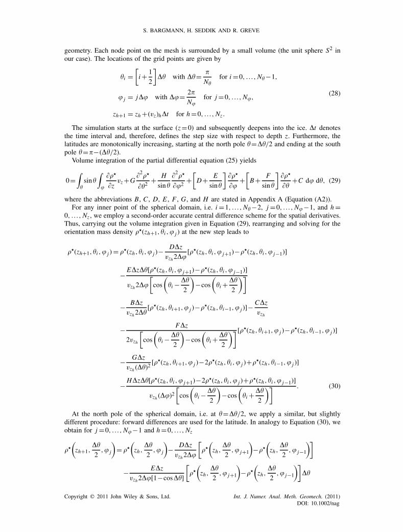
geometry. Each node point on the mesh is surrounded by a small volume (the unit sphere S2 inour case). The locations of the grid points are given by

i =[i+ 1

2

]� with �= �

Nfor i =0, . . . ,N−1,

j = j� with �= 2�

Nfor j=0, . . . ,N,

zh+1 = zh +(vz)h�t for h=0, . . . ,Nz .

(28)

The simulation starts at the surface (z=0) and subsequently deepens into the ice. �t denotesthe time interval and, therefore, defines the step size with respect to depth z. Furthermore, thelatitudes are monotonically increasing, starting at the north pole =�/2 and ending at the southpole =�−(�/2).

Volume integration of the partial differential equation (25) yields

0=∫sin

∫

��

�zvz+G

�2��

�2+ H

sin

�2��

�2+

[D+ E

sin

]��

�+

[B+ F

sin

]��

�+C d d, (29)

where the abbreviations B, C , D, E , F , G, and H are stated in Appendix A (Equation (A2)).For any inner point of the spherical domain, i.e. i =1, . . . ,N−2, j =0, . . . ,N −1, and h=

0, . . . ,Nz , we employ a second-order accurate central difference scheme for the spatial derivatives.Thus, carrying out the volume integration given in Equation (29), rearranging and solving for theorientation mass density ��(zh+1,i , j ) at the new step leads to

��(zh+1,i , j )= ��(zh ,i , j )−D�z

vzh2�[��(zh ,i , j+1)−��(zh ,i , j−1)]

− E�z�[��(zh ,i , j+1)−��(zh ,i , j−1)]

vzh2�

[cos

(i − �

2

)−cos

(i + �

2

)]

− B�z

vzh2�[��(zh ,i+1, j )−��(zh ,i−1, j )]−

C�z

vzh

− F�z

2vzh

[cos

(i − �

2

)−cos

(i + �

2

)] [��(zh ,i+1, j )−��(zh ,i−1, j )]

− G�z

vzh (�)2[��(zh ,i+1, j )−2��(zh ,i , j )+��(zh ,i−1, j )]

−H�z�[��(zh ,i , j+1)−2��(zh ,i , j )+��(zh ,i , j−1)]

vzh (�)2[cos

(i − �

2

)−cos

(i + �

2

)] . (30)

At the north pole of the spherical domain, i.e. at =�/2, we apply a similar, but slightlydifferent procedure: forward differences are used for the latitude. In analogy to Equation (30), weobtain for j =0, . . . ,N−1 and h=0, . . . ,Nz

��

(zh+1,

�

2, j

)= ��

(zh ,

�

2, j

)− D�z

vzh2�

[��

(zh,

�

2, j+1

)−��

(zh ,

�

2, j−1

)]

− E�z

vzh2�[1−cos�]

[��

(zh ,

�

2, j+1

)−��

(zh ,

�

2, j−1

)]�



− B�z

vzh�

[1

2��

(zh ,

3�

2, j

)+ 1

2��

(zh ,

�

2, j

)− 1

N

N−1∑l=0

��

(zh ,

�

2,l

)]

−C�z

vzh− F�z

vzh [1−cos�]

[1

2��

(zh,

3�

2, j

)+ 1

2��

(zh ,

�

2, j

)

− 1

N

N−1∑l=0

��

(zh,

�

2,l

)]− G�z

vzh (�)2

[1

4��

(zh ,

5�

2, j

)

+1

2��

(zh ,

3�

2, j

)+ 1

4��

(zh ,

�

2, j

)− 1

N

N−1∑l=0

��

(zh ,

�

2,l

)]

− H�z�

vzh [1−cos�](�)2

[��

(zh ,

�

2, j+1

)

−2��

(zh,

�

2, j

)+��

(zh,

�

2, j−1

)]. (31)

At the south pole (=�−(�/2)), backward differences are applied for the latitude,

��

(zh+1,�− �

2, j

)= ��

(zh ,�− �

2, j

)

− D�z

vzh2�

[��

(zh ,�− �

2, j+1

)−��

(zh,�− �

2, j−1

)]

− E�z

vzh2�[1−cos�]

[��

(zh ,�− �

2, j+1

)−��

(zh ,�− �

2, j−1

)]�

− B�z

vzh�

[1

N

N−1∑l=0

��

(zh,�− �

2,l

)

−1

2��

(zh ,�− 3�

2, j

)− 1

2��

(zh ,�− �

2, j

)]− C�z

vzh

− F�z

vzh [1−cos�]

[1

N

N−1∑l=0

��

(zh,�− �

2,l

)

−1

2��

(zh ,�− 3�

2, j

)− 1

2��

(zh ,�− �

2, j

)]

− G�z

vzh (�)2

[1

N

N−1∑l=0

��

(zh ,�− �

2,l

)− 1

4��

(zh ,�− 5�

2, j

)

−1

2��

(zh ,�− 3�

2, j

)− 1

4��

(zh ,�− �

2, j

)]

− H�z�

vzh [1−cos�](�)2

[��

(zh,�− �

2, j

)

−2��

(zh ,�− �

2, j−1

)+��

(zh�−,

�

2, j−2

)]. (32)



This provides a complete set of discretized equations for the EDML ice. The advantage of thediscretization scheme described above is that no boundary conditions are required at the two poles.This clearly makes sense because in reality the poles are just an ordinary grid point of the unitsphere. Moreover, the singularity of Equation (25) does not cause any problems.

For the results presented in Section 5, the angular resolution of the unit sphere is discretized asstated in Equation (28) is �=�=5◦. Moreover, � t=1 day is chosen for the time step.

5. RESULTS

Figure 11 depicts preliminary fabric data from the Antarctic EDML ice core (I. Weikusat,personal communication 2007 and 2009, partly published by [1]). Near the surface the ice isisotropic. Below ∼600 m depth a broad girdle fabric forms, and it narrows gradually downto ∼2000 m depth. A sudden change in the flow regime is indicated by a vertical alignmentof the c-axes over ∼10 m to a single maximum fabric at ∼2040 m depth. Further down,the single maximum essentially prevails. All single maxima show a small, but noticeabledeviation from the vertical (center of the Schmidt diagrams). No data are available for the

Figure 11. Orientation distributions for different samples of the EDML ice core between depths of 54 and2556 m (I. Weikusat, personal communication, 2007 and 2009, partly published by [1]). The centers of theSchmidt diagrams coincide with the core axis. The data originate from vertically cut thin sections, rotatedto the horizontal view. The quantity n denotes the number of grains included. During the drilling process,the orientation of the samples in the horizontal plane could not be maintained, so that it is unknown.



0 0.2 0.4 0.6 0.8 1

0

500

1000

1500

2000

2500

3000

s a11

s a22

s a33

d a11

d a22

d a33

Orientation tensor

Dep

th[m

]

0 0.2 0.4 0.6 0.8 1

0

500

1000

1500

2000

2500

3000

s a11

s a22

s a33

d a11

d a22

d a33

Orientation tensor

Dep

th[m

]

0 0.2 0.4 0.6 0.8 1

0

500

1000

1500

2000

2500

3000

s a11

s a22

s a33

d a11

d a22

d a33

Orientation tensor

Dep

th[m

]

Figure 12. Simulated profiles of the three diagonal elements a11, a22, and a33 (labeled ‘s aii’) of thesecond-order orientation tensor along the EDML ice core. Top left panel: �=0, �=0. Top right panel:�=10−15 s−1, �=0. Bottom panel: �=10−13 s−1, �=0. For comparison, the profiles computed from the

fabric data of Figure 11 are shown (labeled ‘d aii’).

bottom-most ∼200 m of the ice core. For a more detailed discussion of the data we refer to Eisenet al. [49].

We have carried out a series of simulations with the model described above (Sections 3 and 4).The parameters listed in Table I are the same as those used in the previous study by Seddiket al. [1] with the exception of the updated value for the horizontal extension ratio a and the newparameters � (orientation diffusivity) and � (orientation production parameter). For the two latter,starting from the initial guess made in the remark at the end of Section 2.1, we have tried valuesof 0, 10−16, 10−15, 10−14, 10−13, 10−12, and 10−11 s−1. Selected results of this parameter studywill be presented in the following.

Figure 12 shows the simulated profiles of the three diagonal elements a11, a22, and a33 ofthe second-order orientation tensor a(2) along the EDML ice core for three different valuesof �(0,10−15,10−13 s−1) and �=0. The second-order orientation tensor is the second moment ofthe ODF,

a(2)(x, t)=∫S2

f �(x, t,n)(n⊗n) d2n. (33)

It is symmetric, the trace a11+a22+a33 is equal to unity, and for an isotropic fabric it is equalto 1/3 times the unit tensor. A large value of a33 represents a concentration of the c-axes inthe vertical direction, and an ideal vertical single maximum fabric would result in a33→1. Theelements a11 and a22 indicate the symmetry with respect to the vertical direction, in the sense that



a11=a22 denotes transverse isotropy (circular symmetry in the horizontal plane), while |a11−a22|represents the degree of deviation from transverse isotropy.

All three simulations show a monotonic increase of a33 and decrease of a11 and a22 fromisotropic conditions at the surface to a single maximum fabric at ∼2000 m depth. Except for somefine structure, for the two cases �=0 and �=10−15 s−1 the agreement of a33 with the fabric data isvery good, and the agreement of a11 and a22 is moderate (the large difference of |a11−a22| in thedata is only partly reproduced by the simulations). Further down, in the region where shear flowbecomes predominant, the agreement worsens. The simulations produce some oscillatory behavioraround an average value of a33∼0.7, while the data show a significantly stronger single maximum.The oscillations are less pronounced for �=10−15 s−1 than for �=0; otherwise, the results of thesetwo simulations are very similar.

The agreement between simulated and observed fabrics is clearly reduced for the simulationwith �=10−13 s−1. For this case, the diffusive process of rotation recrystallization weakens thesimulated anisotropy too much, and consequently, orientation diffusivities ��10−13 s−1 must bediscarded. For �=10−14 s−1 (not shown), the agreement with the data is still acceptable; however,the oscillations below ∼2000 m depth are much stronger than for �=10−15 s−1. Because of thesefindings, we take the latter value as our reference value.

The next step is to investigate the influence of the orientation production parameter �. Figures 12(top right panel) and 13 show the profiles of a11, a22, and a33 for the reference value of theorientation diffusivity � (10−15 s−1) and three different values of � (0, 10−13, 10−11 s−1). Owing tothe temperature-dependent formulation in Equation (9), which reflects the fact that grain boundarymigration is more efficient at high temperatures, variations of � mainly affect the lower parts of theprofile. The results for �=0 and �=10−13 s−1 are very similar except for the reduced near-bottomoscillations in the case �=10−13 s−1. By contrast, �=10−11 s−1 produces too strong anisotropies(too large values of a33) at intermediate depths (∼1250–2000 m) and a too strong decrease of theanisotropy further down. The latter holds to a lesser extent also for the case �=10−12 s−1 (notshown). Consequently, we discard orientation production parameters ��10−12 s−1, and take thevalue �=10−13 s−1 as our reference value.

In the following, the simulation with the reference values for the orientation diffusivity, �=10−15 s−1, and the orientation production parameter, �=10−13 s−1, is referred to as the referencesimulation. Detailed Schmidt diagram representations of the fabrics (ODF) that lead to the profilesof a11, a22, and a33 shown in Figure 13 (left panel) are depicted in Figure 14. For the sake of easycomparison with the fabric data, the depths are the same as in Figure 11.

0 0.2 0.4 0.6 0.8 1

0

500

1000

1500

2000

2500

3000

s a11

s a22

s a33

d a11

d a22

d a33

Orientation tensor

Dep

th[m

]

0 0.2 0.4 0.6 0.8 1

0

500

1000

1500

2000

2500

3000

s a11

s a22

s a33

d a11

d a22

d a33

Orientation tensor

Dep

th[m

]

Figure 13. Simulated profiles of the three diagonal elements a11, a22, and a33 (labeled ‘s aii’) of thesecond-order orientation tensor along the EDML ice core. Left panel: �=10−15 s−1, �=10−13 s−1 (refer-ence simulation). Right panel: �=10−15 s−1, �=10−11 s−1. For comparison, the profiles computed from

the fabric data of Figure 11 are shown (labeled ‘d aii’).



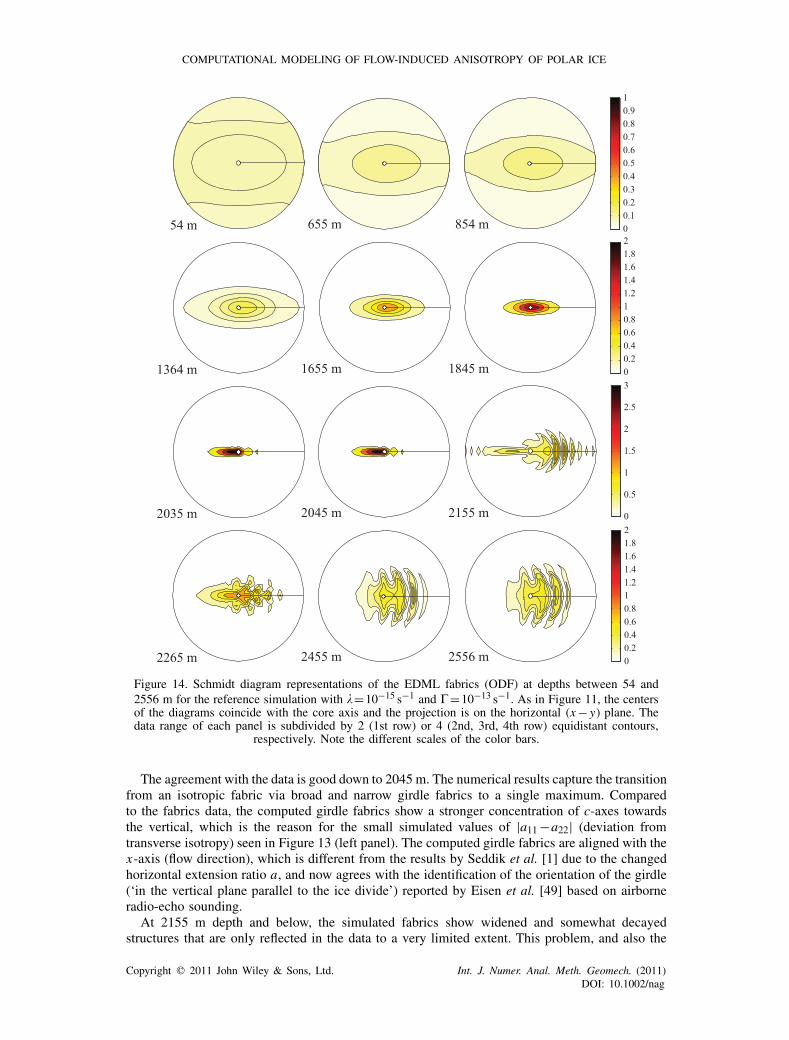
Figure 14. Schmidt diagram representations of the EDML fabrics (ODF) at depths between 54 and2556 m for the reference simulation with �=10−15 s−1 and �=10−13 s−1. As in Figure 11, the centersof the diagrams coincide with the core axis and the projection is on the horizontal (x− y) plane. Thedata range of each panel is subdivided by 2 (1st row) or 4 (2nd, 3rd, 4th row) equidistant contours,

respectively. Note the different scales of the color bars.

The agreement with the data is good down to 2045 m. The numerical results capture the transitionfrom an isotropic fabric via broad and narrow girdle fabrics to a single maximum. Comparedto the fabrics data, the computed girdle fabrics show a stronger concentration of c-axes towardsthe vertical, which is the reason for the small simulated values of |a11−a22| (deviation fromtransverse isotropy) seen in Figure 13 (left panel). The computed girdle fabrics are aligned with thex-axis (flow direction), which is different from the results by Seddik et al. [1] due to the changedhorizontal extension ratio a, and now agrees with the identification of the orientation of the girdle(‘in the vertical plane parallel to the ice divide’) reported by Eisen et al. [49] based on airborneradio-echo sounding.

At 2155 m depth and below, the simulated fabrics show widened and somewhat decayedstructures that are only reflected in the data to a very limited extent. This problem, and also the



0 2 4 6 8 10

0

500

1000

1500

2000

2500

3000

simulationfabric data

Enhancement factor

Dep

th[m

]

0 0.5 1 1.5 2

0

500

1000

1500

2000

2500

3000

simulationfabric data

Horizontal velocity [m/a]

Dep

th[m

]

Figure 15. Simulated profiles of the enhancement factor E (left panel) and the horizontal velocity vx(right panel) along the EDML ice core for the reference simulation with �=10−15 s−1 and �=10−13 s−1.

For comparison, the profiles computed from the fabric data of Figure 11 are shown.

spurious spatial oscillations seen in the simulated fabrics, already came up in the results by Seddiket al. [1], and it is probably influenced by a numerical instability of the finite volume scheme inthis region where shear flow is dominant.

Profiles of the enhancement factor E and the horizontal velocity vx for the reference simulationare shown in Figure 15, along with the corresponding profiles computed from the fabric dataof Figure 11. The decrease of E from unity at the surface to values �0.25 in the region above2000 m depth dominated by vertical compression is well reproduced, as well as the rather abruptincrease to values >2 at ∼2000 m depth where shear flow becomes more dominant. However,related to the problems with the simulated fabrics discussed above, the simulated maximum valueof ∼3 contrasts with the maximum value of ∼8 that results from the fabric data. This entails adiscrepancy in the horizontal velocity profiles; while the simulated profile shows a surface velocityof ∼1.1m/a, the fabric data-based profile shows a surface velocity of ∼1.8m/a. On the otherhand, direct measurements reported by Wesche et al. [2] provide a lower value of 0.756m/adirectly at the drilling site, and values between 0.62 and 0.96m/a at 12 survey points in thevicinity.

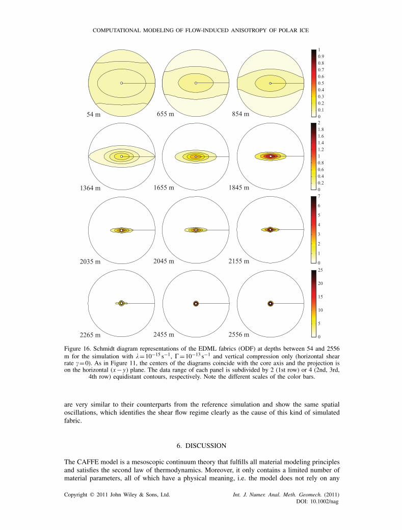
In order to separate the effects of the two deformation regimes of vertical compression andsimple shear, we ran two further simulations; each of them neglecting one of the two deforma-tion regimes. The vertical compression only case is defined by ignoring the horizontal shear rate,i.e. by setting �=0. Schmidt diagrams of the resulting fabrics (ODF) are depicted in Figure 16.They are very similar to those of the reference simulation (Figure 14) down to 2045 m, wherevertical compression dominates the flow regime. Small differences are that in the vertical compres-sion only case the fabric evolution towards a single maximum is slightly slower (well visiblein the diagrams for 2035 and 2045 m), and that the fabrics show a perfect rotational symmetrywith respect to the vertical, while the symmetry is slightly broken in the reference simula-tion (see mainly the diagrams for 854, 1364, and 1655m depth). Below 2045m, the singlemaximum fabric of the vertical compression only case strengthens further towards an almostideal vertical single maximum, whereas, under the influence of shear-dominated deformation, thereference simulation produces the widened and somewhat decayed structures already mentionedabove.

The simple shear only case is realized by ignoring the vertical compression rate, i.e. by setting�=0. For this case, the Schmidt diagrams are shown in Figure 17. Down to 1845 m, the fabricremains almost isotropic, with two very weak maxima 45◦ off the vertical in ±x-direction (alignedwith the flow direction). From 2035 m on, the fabric is significantly anisotropic, the maximumin −x-direction disappears, and the maximum in +x-direction moves closer towards the verticalunder the influence of grain boundary migration. The last two diagrams for 2455 and 2556m



Figure 16. Schmidt diagram representations of the EDML fabrics (ODF) at depths between 54 and 2556m for the simulation with �=10−15 s−1, �=10−13 s−1 and vertical compression only (horizontal shearrate �=0). As in Figure 11, the centers of the diagrams coincide with the core axis and the projection ison the horizontal (x− y) plane. The data range of each panel is subdivided by 2 (1st row) or 4 (2nd, 3rd,

4th row) equidistant contours, respectively. Note the different scales of the color bars.

are very similar to their counterparts from the reference simulation and show the same spatialoscillations, which identifies the shear flow regime clearly as the cause of this kind of simulatedfabric.

6. DISCUSSION

The CAFFE model is a mesoscopic continuum theory that fulfills all material modeling principlesand satisfies the second law of thermodynamics. Moreover, it only contains a limited number ofmaterial parameters, all of which have a physical meaning, i.e. the model does not rely on any



Figure 17. Schmidt diagram representations of the EDML fabrics (ODF) at depths between 54 and 2556m for the simulation with �=10−15 s−1, �=10−13 s−1 and simple shear only (vertical compression rate�=0). As in Figure 11, the centers of the diagrams coincide with the core axis and the projection is onthe horizontal (x− y) plane. The data range of each panel is subdivided by 2 (1st, 2nd row) or 4 (3rd,

4th row) equidistant contours, respectively. Note the different scales of the color bars.

artificial parameters. The introduction of an ODF as a statistical measurement, instead of evaluatingthe mesoscopic space directly, is numerically very efficient. Further, the enhancement factor Eaccounting for the anisotropy of the ice is a scalar quantity. This is opposed to many other theoriesthat introduce tensorial quantities of second or fourth order to account for anisotropic effects.Consequently, the CAFFE model is suitable for implementation in ice flow models of all kindsof complexity. While the full version of the model as presented here still leads to two additionaldegrees of freedom (the polar and azimuth angles of the unit sphere that represents the orientationspace), the model can be simplified further by replacing the fabric evolution equation (3) by anevolution equation for the second-order orientation tensor a(2) as defined in Equation (33) anda closure condition for the fourth-order orientation tensor (see Seddik et al. [28]). In this case,



no additional degrees of freedom emerge, and the additional computational effort for the CAFFEmodel is relatively small.

In this paper, the CAFFE model was applied to the ice of the EDML deep drilling site. Theprevious study by Seddik et al. [1] already showed that the CAFFE model is capable of reproducingessential characteristics of the anisotropic ice flow at the site of the EDML ice core. However, intheir study only local rigid body rotation and grain rotation were accounted for, and the assumedvalue of the horizontal extension ratio turned out not to agree with measured data of the strainregime at the ice surface [2]. Our study extends this work by proposing suitable parameterizationsfor rotation recrystallization and grain boundary migration, and adopting a horizontal extensionratio that agrees with the mentioned observations. The latter brings the simulated orientation of thegirdle fabric above ∼2000 m depth in agreement with the interpretation of radio-echo soundings[49]. Based on comparisons between simulated and observed fabrics, we provided reference valuesfor the parameters that appear in the constitutive equations for rotation recrystallization and grainboundary migration. Additionally, the effects of the two underlying deformation regimes of verticalcompression and simple shear were examined separately in order to study their respective influenceson the simulated fabrics.

Some limitations of this study must be noted, which arise mainly from the simplicity of the flowmodel. The restriction to one spatial dimension (the vertical) was already justified by Seddik et al.[1] by stating that ‘the variation of the shear upstream of the drill site is probably small due tothe small variation of the surface gradient, so that the error resulting from the neglected horizontalinhomogeneity should be limited’. Nevertheless, variable ice thicknesses and vertical compressionrates upstream will have some influence on the flow regime of the ice at the EDML drillingsite, and thus on the computed fabric profile. Our steady-state assumption introduces a furthersource of uncertainty, since the real ice sheet has been exposed to varying climatic conditionsover glacial/interglacial cycles on time scales of 10s to 100s of thousands of years as well asto climate change events on shorter time scales (e.g. Wilson et al. [51]). A further simplificationis the assumption of no-slip conditions (zero horizontal velocity) at the ice base. Since the basaltemperature is at the pressure melting point, one would expect some amount of basal sliding tobe present (e.g. Paterson [40]). However, if basal sliding contributed significantly to the horizontalvelocity at the EDML drilling site, the measured surface velocity should exceed the simulated one.As we have seen above, the opposite is true, and so it seems that basal sliding is indeed negligible.

To conclude, the CAFFE model represents a good compromise between physical adequacy andsimplicity. By including the effects of rotation recrystallization and grain boundary migration innumerical simulations and proposing suitable parameters for the constitutive equations of theseeffects, our study constitutes a step forward to developing the CAFFE model as a useful tool forice flow modeling. Robustness of numerical schemes for solving the CAFFE model equations isstill an issue and requires further efforts.

APPENDIX A

The fabric evolution equation, Equation (25), can be written in the abbreviated form

0= ��(z,,)

�zvz(z)+G(,)

�2��(,)

�2+ H (,)

sin

�2��(,)

�2

+[D(,)+ 1

sinE(,)

]��(,)

�

+[B(,)+ F(,)

sin

]��(,)

�+C(,) (A1)



with the functions

B = 1

2

[−1

2�ε sin2[[2a−1]cos2+3]+�[1−�cos2]cos

],

C = 3

4��[ε[[4a−2]sin2 cos2−1−3cos2]+2�sin2cos]

−��A(T ′)

A(−10◦C)[A�−A],

D = 1

2ε�[2a−1]sin2,

E = 1

2�[�−1]

sin

tan,

F = −�cos,

G = −�,

H = − �

sin.

(A2)

ACKNOWLEDGEMENTS

We thank I. Weikusat and S. Kipfstuhl for their collaboration and communications on the fabric data,F. Wilhelms for providing the measured temperature profile, and I. Weikusat and O. Eisen (all at theAlfred Wegener Institute for Polar and Marine Research, Bremerhaven, Germany) for helpful discussions.Comments of the scientific editor S. Sture, the reviewer K. Hutter, and two anonymous reviewers helpedconsiderably to improve the clarity and writing of the manuscript.

S.B. was supported by grant BA 3951/1 of the German Science Foundation (DFG), which is gratefullyacknowledged. This research was done while S.B. visited the Institute of Low Temperature Science,Hokkaido University.

REFERENCES

1. Seddik H, Greve R, Placidi L, Hamann I, Gagliardini O. Application of a continuum-mechanical model for theflow of anisotropic polar ice to the EDML core, Antarctica. Journal of Glaciology 2008; 54(187):631–642.

2. Wesche C, Eisen O, Oerter H, Schulte D, Steinhage D. Surface topography and ice flow in the vicinity of theEDML deep-drilling site, Antarctica. Journal of Glaciology 2007; 53(182):442–448.

3. Bamber JL, Bindschadler RA. An improved elevation dataset for climate and ice-sheet modelling: validation withsatellite imagery. Annals of Glaciology 1997; 25:439–444.

4. Placidi L. Thermodynamically consistent formulation of induced anisotropy in polar ice accounting for grain-rotation, grain-size evolution and recrystallization. Doctoral Thesis, Darmstadt University of Technology, 2004.

5. Placidi L, Greve R, Seddik H, Faria SH. A continuum-mechanical, anisotropic flow model for polar ice,based on an anisotropic flow enhancement factor. Continuum Mechanics and Thermodynamics 2010; 22(3):221–237.

6. Huybrechts P, Rybak O, Pattyn F, Ruth U, Steinhage D. Ice thinning, upstream advection, and non-climaticbiases for the upper 89% of the EDML ice core from a nested model of the Antarctic ice sheet. Climate of thePast 2007; 3(4):577–589.

7. Saito F, Abe-Ouchi A. Thermal structure of Dome Fuji and east Dronning Maud Land, Antarctica, simulated bya threedimensional ice-sheet model. Annals of Glaciology 2004; 39:433–438.

8. Morland LW, Staroszczyk R. Viscous response of polar ice with evolving fabric. Continuum Mechanics andThermodynamics 1998; 10:135–152.

9. Morland LW, Staroszczyk R. Stress and strain-rate formulations for fabric evolution in polar ice. ContinuumMechanics and Thermodynamics 2003; 15(1):55–71.

10. Gillet-Chaulet F, Gagliardini O, Meyssonnier J, Montagnat M, Castelnau O. A user-friendly anisotropic flow lawfor ice sheet modelling. Journal of Glaciology 2005; 51(172):3–14.

11. Gillet-Chaulet F, Gagliardini O, Meyssonnier J, Zwinger T, Ruokolainen J. Flow-induced anisotropy in polar iceand related ice-sheet flow modelling. Journal of Non-Newtonian Fluid Mechanics 2006; 134(1–3):33–43.



12. Lliboutry L. Anisotropic, transversely isotropic nonlinear viscosity of rock ice and rheological parameters inferredfrom homogenization. International Journal of Plasticity 1993; 9(5):619–632.

13. Azuma N. A flow law for anisotropic polycrystalline ice under uniaxial compressive deformation. Cold RegionsScience and Technology 1995; 23(2):137–147.

14. Castelnau O, Thorsteinsson T, Kipfstuhl J, Duval P, Canova GR. Modelling fabric development along the GRIPice core, central Greenland. Annals of Glaciology 1996; 23:194–201.

15. Castelnau O, Shoji H, Mangeney A, Milsch H, Duval P, Miyamoto A, Kawada K, Watanabe O. Anisotropicbehavior of GRIP ices and flow in central Greenland. Earth and Planetary Science Letters 1998; 154(1–4):307–322.

16. Svendsen B, Hutter K. A continuum approach for modelling induced anisotropy in glaciers and ice sheets. Annalsof Glaciology 1996; 23:262–269.

17. Gödert G, Hutter K. Induced anisotropy in large ice shields: theory and its homogenization. Continuum Mechanicsand Thermodynamics 1998; 10(5):293–318.

18. Ktitarev D, Gödert G, Hutter K. Cellular automaton model for recrystallization, fabric, and texture developmentin polar ice. Journal of Geophysical Research 2002; 107(B8):265.

19. Thorsteinsson T. Fabric development with nearest-neighbour interaction and dynamic recrystallization. Journalof Geophysical Research 2002; 107(B1):2014.

20. Staroszczyk R. A multi-grain model for migration recrystallization in polar ice. Archives of Mechanics 2009;61(3–4):259–282.

21. Meyssonnier J, Philip A. Comparison of finite-element and homogenization methods for modelling the viscoplasticbehaviour of a S2-columnar-ice polycrystal. Annals of Glaciology 2000; 30:115–120.

22. Mansuy P, Meyssonnier J, Philip A. Localization of deformation in polycrystalline ice: experiments and numericalsimulations with a simple grain model. Computational Materials Science 2002; 25(1–2):142–150.

23. Lebensohn RA, Liu Y, Ponte Castañeda P. Macroscopic properties and field fluctuations inmodel power-lawpolycrystals: full-field solutions versus self-consistent estimates. Proceedings of the Royal Society A 2004;460(2045):1381–1405.

24. Lebensohn RA, Liu Y, Ponte Castañeda P. On the accuracy of the self-consistent approximation for polycrystals:comparison with full-field numerical simulations. Acta Materialia 2004; 52(18):5347–5361.

25. van der Veen CJ. Development of fabric in ice. Cold Regions Science and Technology 1994; 22:171–195.26. Gagliardini O, Gillet-Chaulet F, Montagnat M. A review of anisotropic polar ice models: from crystal to ice-sheet

flow models. Low Temperature Science 2009; 68:149–166. (Supplement Issue ‘Physics of Ice Core Records II’,T. Hondoh (ed.)).

27. Faria SH. The symmetry group of the CAFFE model. Journal of Glaciology 2008; 54(187):643–645.28. Seddik H, Greve R, Zwinger T, Placidi L. A full-Stokes ice flow model for the vicinity of Dome Fuji, Antarctica,

with induced anisotropy and fabric evolution. The Cryosphere Discussions 2009; 3(1):1–31.29. Azuma N, Higashi A. Formation processes of ice fabric pattern in ice sheets. Annals of Glaciology 1985;

6:130–134.30. Gow AJ, Williamson T. Rheological implications of the internal structure and crystal fabrics of the West Antarctic

ice sheet as revealed by deep core drilling at Byrd Station. CRREL Report 1976; 76(35):1665–1677.31. Placidi L, Hutter K. Thermodynamics of polycrystalline materials treated by the theory of mixtures with continuous

diversity. Continuum Mechanics and Thermodynamics 2006; 17(6):409–451.32. Dafalias YF. Orientation distribution function in non-affine rotations. Journal of the Mechanics and Physics of

Solids 2001; 49:2493–2516.33. Fick A. On liquid diffusion. Philosophical Magazine 1855; 10:30–39.34. Humphreys FJ, Hatherly M. Recrystallization and Related Annealing Phenomena. Elsevier: Amsterdam, 2004.35. Poirier J-P. Creep of Crystals. Cambridge University Press: Cambridge, 1985.36. Weertman J, Weertman JR, Elementary Dislocation Theory. Oxford University Press: Oxford, 1992.37. Montagnat M, Duval P. Rate controlling processes in the creep of polar ice: influence of grain boundary migration

associated with recrystallization. Earth and Planetary Science Letters 2000; 183(1–2):179–186.38. Greve R, Blatter H. Dynamics of Ice Sheets and Glaciers. Springer: Berlin, Germany, 2009.39. Kamb B. Experimental recrystallization of ice under stress. In Flow and Fracture of Rocks, Heard HC, Borg IY,

Carter NL, Raileigh CB (eds). American Geophysical Union: Washington, DC, 1972; 211–241.40. Paterson WSB. The Physics of Glaciers, (3rd edn). Pergamon Press: Oxford, 1994.41. Glen JW. The creep of polycrystalline ice. Proceedings of the Royal Society A 1955; 228:519–538.42. Hooke LeB R. Principles of Glacier Mechanics (2nd edn). Cambridge University Press: Cambridge, 2005.43. Miyamoto A. Mechanical properties and crystal textures of Greenland deep ice cores. Doctoral Thesis, Hokkaido

University, 1999.44. Budd WF, Jacka TH. A review of ice rheology for ice sheet modelling. Cold Regions Science and Technology

1989; 16(2):107–144.45. Pimienta P, Duval P, Lipenkov VY. Mechanical behaviour of anisotropic polar ice. In The Physical Basis of Ice

Sheet Modelling, IAHS Publication No. 170, Waddington ED, Walder JS (eds). IAHS Press: Wallingford, U.K.,1987; 57–66.

46. Russell-Head DS, Budd WF. Ice sheet flow properties derived from borehole shear measurements combined withice core studies. Journal of Glaciology 1979; 24(90):117–130.



47. Dansgaard W, Johnsen SJ. A flow model and a time scale for the ice core from Camp Century, Greenland.Journal of Glaciology 1969; 8(53):215–223.

48. Wilhelms F, Sheldon SG, Hamann I, Kipfstuhl S. Implications for and findings from deep ice core drillings—Anexample: the ultimate tensile strength of ice at high strain rates. In Physics and Chemistry of Ice, SpecialPublication No. 311, Kuhs WF (ed.). The Royal Society of Chemistry: Cambridge, U.K., 2007; 635–639.

49. Eisen O, Kipfstuhl S, Steinhage D, Wilhelms F. Direct evidence for continuous radar reflector originating fromchanges in crystal-orientation fabric. The Cryosphere 2007; 1(1):1–10.

50. van der Veen CJ. Fundamentals of Glacier Dynamics. AA Balkema: Rotterdam, The Netherlands, 1999.51. Wilson RCL, Drury SA, Chapman JL. Climate change and life. The Great Ice Age. Routledge: London and

New York, 2000.


Computational modeling of flow-induced anisotropy of polar ice for the EDML deep drilling site,...

Documents

Transcript of Computational modeling of flow-induced anisotropy of polar ice for the EDML deep drilling site,...