Nonlinear Analysis of PrandtlPlane Joined Wings: Effects of Anisotropy

Nonlinear Analysis of PrandtlPlane Joined Wings -

Part II: Effects of Anisotropy

Rauno Cavallaro,∗ Luciano Demasi ††, Andrea Passariello ‡‡

Structural geometrical nonlinearities strongly affect the response of PrandtlPlane JoinedWings: it has been shown that linear buckling evaluations are unreliable and only a fullynonlinear stability analysis can safely identify the unstable state. This work focuses onthe understanding of the main physical mechanisms driving the wing system’s responseand the snap-buckling instability. Several counterintuitive effects typical of unconventionalnon-planar wing systems are discussed and explained. In particular, an appropriate designof the joint-to-wing connection may reduce the amount of bending moment transferred, andthis is shown to dramatically improve the stability properties. It is also demonstrated thatthe lower-to-upper-wing stiffness ratio and the torsional-bending coupling, due to both thegeometrical layout and anisotropy of the composite laminates, present a major impact onthe nonlinear response. How the material anisotropy modifies the Snap Buckling Regionand the response is also discussed.The findings of this work could provide useful indications to develop effective aeroelasticreduced order models tailored for airplanes experiencing important geometric nonlinearitiessuch as PrandtlPlane aircraft, Truss-braced and Strut-Braced wings and sensorcrafts.

I. Introduction

JOINED Wings were proposed in the seventies1–3 for commercial transport and supersonic fighters. JoinedWings were also the subject of US4,5 and European6,7 patents. Many advantages are claimed compared

to classical cantilevered configurations:8–12 improved stiffness properties, high aerodynamic efficiency13 andsuperior stability and control characteristics. In addition to these theoretically significant advantages, adiamond Joined Wing can enclose a large antenna and be used for high altitude surveillance.14,15

For civil transportation, the PrandtlPlane5,8 has been analyzed in terms of aerodynamic performances,13,16–18

flight mechanics and controls,10 dynamic aeroelastic stability properties19 and preliminary design.20 More-over, several PrandtlPlane-like Joined Wings were also proposed for example for the design of UnmannedAir Vehicles.9

The design of Joined-Wing type of aircraft for civil transportation was also adopted in United States withthe introduction of the concept of Strut-Braced Wings (SBW)21,22 and Truss Braced Wings (TBW).23

The growth of interest on Joined Wings led to both experimental24,25 and theoretical26–28 studies. Thesestudies showed that the tools developed in decades and effectively used by the industry to analyze classicalcantilevered wings need to take into account structural nonlinearities29–31 which are significant even forsmall angles of attack and attached flow. The strong in-plane forces transferred through the joint make thegeometric structural effects particularly important and linear aeroelastic models32 can give only a qualitativeinformation on the instability properties but may miss important structural effects which should be taken intoaccount.33,34 However, the adoption of fully-nonlinear structural models is impractical for design purposesespecially if several alternative configurations are explored in an optimization32 effort. Ideally, one shouldhave an efficient aeroelastic model tailored for optimization strategies. With this in mind and consideringthat the main physical aspect for a preliminary design of Joined Wings is the structural nonlinearity even at

∗PhD Candidate, Department of Aerospace Engineering and Engineering Mechanics, San Diego State University and De-partment of Structural Engineering, University of California San Diego

†Assistant Professor, Department of Aerospace Engineering and Engineering Mechanics, San Diego State University, AIAAMember

‡Visiting Graduate Student, San Diego State University, MS Candidate at the Dipartimento di Ingegneria Aerospaziale,Universita di Pisa

1 of 37

American Institute of Aeronautics and Astronautics

53rd AIAA/ASME/ASCE/AHS/ASC Structures, Structural Dynamics and Materials Conference<BR>20th AI23 - 26 April 2012, Honolulu, Hawaii

AIAA 2012-1462

Copyright © 2012 by Rauno Cavallaro, Luciano Demasi, Andrea Passariello. Published by the American Institute of Aeronautics and Astronautics, Inc., with permission.

small angles of attack, a procedure which coupled the fully nonlinear structural finite element capability anda modally-based aerodynamic solver in the frequency domain was proposed in Reference [35]. This couldbe a valid alternative to the fully coupled nonlinear CFD and CSD models which would be impractical inthe preliminary design of a joined-wing airplane. Ideally, one should be able to describe the fluid-structureinteraction with a reduced order model so that the main physics is well described and yet, the optimizationprocedure can be accurate and fast for the preliminary sizing. The adoption of a detailed nonlinear structuralmodel coupled with a modally-based reduced order aerodynamics has been proven35 successful. However, areduced order model for both aerodynamics and structures would be computationally faster and more indi-cated for the design process. Unfortunately, in the case of Joined Wings the strong structural nonlinearitiesmakes an efficient reduced order model very difficult to achieve. On this regard, in Reference [36] a basis offree vibration modes enriched with a set of second order modes (modal derivatives),37 a promising techniquewhich has been very effective in other problems,38 was adopted. However, the results were not satisfactoryfor the case of Joined Wings. Other techniques could be used to reach the goal of having an efficient andgeneral reduced order aeroelastic capability. For example, the procedures developed in References [39], [40],and [41] could be adopted. However, these methods require (for a basis of just a few modes) several hundredsof fully nonlinear computationally expensive off-line analyses to evaluate some modal stiffness coefficientsadopted to reconstruct the structural behavior. This would not be very practical in the sizing of joined-wingaircrafts and far from an ideal tool for optimization. In Reference [42] an alternative approach based onthe adoption of the Proper Orthogonal Decomposition43–45 (POD) to reconstruct the modes used in thedefinition of the reduced order basis proven to be very effective but only up to the freestream velocity forwhich the POD analysis was performed. The extrapolation techniques for higher velocities did not presentsatisfactory performances.It was then realized that in order to effectively build a reduced order aeroelastic model specifically tailoredfor an efficient simulation with a full inclusion of the structural geometric effects, a physical understandingof the mechanism driving the nonlinear response of Joined Wings should be achieved.For the PrandtlPlane configuration, which showed a strong potential impact on the civil transportation,8

this was pursued in Reference [46]. The main results that were found could be summarized in the followingmain aspects. First, the strong nonlinear structural effects make the linear buckling analysis not very reliableas far as the static critical condition is concerned. Second, the system may be sensitive to snap-bucklingtype of instability under a certain combination of structural parameters. This led to the definition of theso-called Snap-Buckling Region which gives important indications on the design of these airplanes. Third,it was shown that the load repartition between the upper and lower wings has a significant impact on thestability conditions. In fact, it was demonstrated that for a typical swept-back lower wing and swept-forwardupper wing configuration more load on the upper wing alleviates the risk of instability. Fourth, some coun-terintuitive effects typical of this configuration were discovered. For example, increasing the joint’s size maybe considered a not efficient design, since it could increase the height and this would appear unfavorable:it is well known that slender columns may increase the tendency to buckle. However, for aerodynamic-likemechanical loadings it was shown that the complex nonlinear response of the Joined Wing has actually anopposite effect and the stability properties are actually improved when the joint’s height is increased. Thishas also practical implications since the induced drag is significantly reduced when the gap between theupper and lower wing is increased. Fifth, increasing the sweep angles was shown to dramatically reduce thenonlinear buckling load.These findings had relevant practical implications, but several questions needed an answer. In particular, theeffects of composite materials required investigation since additional couplings could be introduced becauseof the anisotropy. Moreover, nowadays the adoption of composites is increasingly relevant (the new Boeing787 and the Airbus 350 present a large percentage of structures designed with composites) and has to beconsidered also for Joined Wings. In addition, even for isotropic materials but general geometries (sweepangles, dihedrals, built-in twist), a realistic PrandtlPlane would present strong anisotropic behavior from aglobal point of view.

In the design of these configurations, an equivalent composite plate model47 could provide importantindications. Thus, the present investigations based on plate-like models for the wings and the joint couldalso provide practical design information. This paper will try to answer the following fundamental questionson the nonlinear response of PrandtlPlane Joined Wings:

• What is the effect of the anisotropy on the nonlinear response? In particular, how is the snap-bucklinginstability affected by the adoption of composite materials?

2 of 37


• What are the effects of the joint-wing connection on the geometrically nonlinear structural behavior?

• What is the main driving mechanism which leads to the instability?

• How is the Snap Buckling Region modified when the anisotropy effects are taken into account?

The present work provides indications on the physical mechanisms of the nonlinear instability for PrandtlPlaneconfigurations and Joined Wings. This could have practical implications in the development of new and ef-ficient aeroelastic reduced order models which could effectively adopt existing and reliable tools already inuse in the aerospace industry but which cannot be directly extended for the Joined Wings without a properunderstanding of the nonlinear phenomena.

II. Nonlinear Structural Model

The geometrically nonlinear finite element48–51 is based on the linear membrane constant strain trian-gle (CST) and the flat triangular plate element (DKT). The structural tangent matrix KT is sum of twocontributions: the elastic stiffness matrix, KE , and the geometrical stiffness matrix, KG. The material’sproperties, and particularly the fiber’s orientation play a role in the elastic stiffness matrix, as will be shownin the next subsection.

The nonlinear governing equations are solved by adopting iterative methods such as Newton-Raphsonand arc length techniques (see Section B). After each iteration a displacement vector is obtained, rigid bodymotion is eliminated from elements and the pure elastic rotations and strains are found.48–51 Using thesequantities the internal forces are updated for the next iteration.

A. The Elastic Stiffness Matrix for Orthotropic Materials

According to the Classical Laminate Theory (CLT), the composite structure is analyzed with an equivalentsingle layer. This is computationally very efficient if the assumptions adopted in the formulation of thetheory are not violated. This means that CLT is an effective tool if the thickness is significantly smaller thanthe other dimensions of the plate/shell structure.The main concepts are here outlined. Consider a multilayered structure. The generic ith ply (sometimes theterms lamina or layer are also adopted to designate the ply) is identified by the so-called material coordinatesystem xi

1, xi2, and xi

3. This coordinate system is a layer-dependent quantity and depends on the orientationof the layer’s fibers. Under the assumption of plane stress state, the constitutive relations for the ith layercan be written as σ11

σ22

σ12

i

=

Q11 Q12 Q16

Q12 Q22 Q26

Q16 Q26 Q66

i ε11ε22

γ12

i

(1)

where σi11 and σi

22 are the in-plane normal stresses, σi12 is the in-plane shear stress, εi11 and εi22 are the

in-plane normal strains and γi12 is the in-plane shear strain. The transverse stresses and strains do not

appear in the plane stress constitutive relations. The terms Qi11, Q

i22, Q

i12, and Qi

66 are the plane stressreduced stiffness coefficients and depend on the elastic modulus Ei

1 referred to the fiber’s direction xi1. The

coefficients also depend on the elastic modulus Ei2 referred to the in-plane direction xi

2. Finally, the reducedstiffness coefficients also depend on the in-plane shear modulus Gi

12 and Poisson’s ratios νi12 and νi21 (theyare in general different). The formal dependency of the coefficients is written below:

Qi11 =

Ei1

(1− νi12νi21)

Qi22 =

Ei2

(1− νi12νi21)

Qi12 =

νi12Ei2

(1− νi12νi21)

Qi16 = Qi

26 = 0

Qi66 = Gi

12 νi21 = νi12Ei

2

Ei1

(2)

If the element coordinate system x, y, z is contained in the plane of the element and is obtained by a rotationϑi about the xi

3 axis, then it is possible to define the layer’s constitutive relations in this coordinate system

3 of 37


as follows: σxx

σyy

σxy

i

=

Q11 Q12 Q16

Q12 Q22 Q26

Q16 Q26 Q66

i εxxεyy

γxy

i

(3)

It should be noted that the new reduced stiffness coefficients Qi

mn are in general not equal to the corre-sponding terms Qi

mn referred to the material coordinate system. Moreover, there are additional coupling

terms represented by the coefficients Qi

16 and Qi

26 which are now non-zero quantities. The Qi

mn terms canbe found as a function of the reduced stiffness coefficients referred to the material coordinate system by a

transformation. For example, term Qi

12 can be shown to be

Qi

12 = (Qi11 +Qi

22 − 4Qi66) sin

2 ϑi cos2 ϑi +Qi12(sin

4 ϑi + cos4 ϑi) (4)

In the Classical Laminate Theory the kinematic assumptions set to zero transverse and shear strains andthe generic normal remains perpendicular to the laminate’s mid-surface even after the deformation takesplace. The consequent displacement field could be used to express the in-plane strains as a function of themembrane normal strains ε0xx and ε0yy, and the membrane shear strain γ0

xy. Moreover, it is possible to showthat the in-plane strains also depend on the curvatures ε1xx, ε

1yy, and γ1

xy. In other words, direct application

of the Classical Laminate Theory leads to the following expressions for the in-plane strains of the ith ply:εixx = ε0xx + zε1xxεiyy = ε0yy + zε1yyγixy = γ0

xy + zγ1xy

(5)

It should be noted that the z coordinate is measured from the plate mid-plane. Moreover, the membranestrains and curvature are not dependent on the layer under consideration. This is the reason why no isuperscript is used to identify the membrane strains and curvatures. Direct substitution of equation 5 intoequation 3 allows one to express the stresses at ply-level as a function of the membrane strains and curvatures:σxx

σyy

σxy

i

=

Q11 Q12 Q16

Q12 Q22 Q26

Q16 Q26 Q66

i ε0xxε0yy

γ0xy

+ z

Q11 Q12 Q16

Q12 Q22 Q26

Q16 Q26 Q66

i ε1xxε1yy

γ1xy

(6)

The thickness integrated forces per unit of length are indicated as Nxx, Nyy, and Nxy and are referred tothe multilayered structure (made of Nl layers) and not to the single lamina. They are defined as follows:Nxx

Nyy

Nxy

=

Nl∑i=1

∫ hi

hi−1

σxx

σyy

σxy

i

dz (7)

Substituting equation 6 into equation 7 and taking into account the fact that the membrane strains andcurvatures do not depend on the actual lamina (so they can be brought outside the integrals along thethickness), the following relation can be written:Nxx

Nyy

Nxy

=

Nl∑i=1

∫ hi

hi−1

Q11 Q12 Q16

Q12 Q22 Q26

Q16 Q26 Q66

i

dz

ε0xxε0yyγ0xy

+

Nl∑i=1

∫ hi

hi−1

z

Q11 Q12 Q16

Q12 Q22 Q26

Q16 Q26 Q66

i

dz

ε1xxε1yyγ1xy

(8)

or Nxx

Nyy

Nxy

=

A11 A12 A16

A12 A22 A26

A16 A26 A66

ε0xxε0yyγ0xy

+

B11 B12 B16

B12 B22 B26

B16 B26 B66

ε1xxε1yyγ1xy

(9)

where the definitions of the terms Amn and Bmn directly follow when equations 8 and 9 are compared.Equation 9 is often written in a more compact form as follows:

N = Aε0 +Bε1 (10)

4 of 37


A is the matrix whose entries Amn are defined extensional stiffnesses and relate the membrane strains withthe thickness integrated forces per unit of length.B is the matrix whose entries Bmn are defined bending-extensional coupling stiffnesses and relate the cur-vatures with the thickness integrated forces per unit of length.Following a similar procedure, it is possible to define the thickness integrated moments per unit of length asfollows: Mxx

Myy

Mxy

=

Nl∑i=1

∫ hi

hi−1

z

σxx

σyy

σxy

i

dz (11)

Carrying out the integration:Mxx

Myy

Mxy

=

B11 B12 B16

B12 B22 B26

B16 B26 B66

ε0xxε0yyγ0xy

+

D11 D12 D16

D12 D22 D26

D16 D26 D66

ε1xxε1yyγ1xy

(12)

which in compact form is written asM = Bε0 +Dε1 (13)

It should be noted that the matrix B (previously discussed) also couples the membrane strains with themoments per unit of length. The matrix D relates the curvatures with the moments per unit of length. Itsentries are the terms Dmn which are defined bending stiffnesses. They are defined as follows:

Dmn =

Nl∑i=1

∫ hi

hi−1

z2 Qi

mndz (14)

Equations 10 and 13 are usually condensed in a single expression:[N

M

]=

[A B

B D

] [ε0

ε1

](15)

It should be noted that the present shell element is a triangular plate element generically oriented in space.In this formulation the rigid body motion is eliminated at element level. Thus, the adoption of small strainis acceptable even if the geometric nonlinearity is taken into account.From now on, x, y, and z will indicate the global coordinate system and not the element coordinate systemas done in the derivations that led to equation 15.Following the procedure described in References [48–51], equation 15 can be used to derive the expressionfor the element’s elastic stiffness matrix Ke

E . Since N and M depend on the entries of the matrices A, B,and D, it is then clear that the fibers’ orientations angles affect the element’s elastic stiffness matrix Ke

E .

B. Iterative Procedure

In this work the wings are subjected to conservative loads indicated with P ext. There are two main iterativeprocedures employed in the present approach: Newton-Raphson and arc length methods.

In the Newton-Raphson solution procedure an increment of external nodal loads is defined. The appliedloads are calculated setting Λ, a dimensionless parameter indicating the fraction of the applied load. Noticethat when this parameter is equal to the unity, then all P ext load is applied to the structure. It holds that:

P stepµstr = Λ · P ext (16)

being µ is the load step. For the nth iteration of a certain load step µ the internal forces F stepµ iternint are

known from the previous iteration and the unbalanced loads P stepµ iternunb are defined as:

P stepµ iternunb = P stepµ

str − F stepµ iternint (17)

The term iteration used here refers to the repetitive refinement of a nonlinear solution for an incrementalload step. The structural tangent matrix K T is calculated by adding the elastic stiffness matrix KE and the

5 of 37


geometric stiffness matrix KG. According to the Full Newton-Raphson strategy (adopted here), the tangent

matrix is evaluated at each iteration of each load step, and the relative matrix will be then K stepµ iternT .

The assembly is conveniently accomplished at element level. The following linear system is then solved andthe displacement vector ustepµ itern can be found:

K stepµ iternT · ustepµ itern = P stepµ itern

unb (18)

Node location coordinates are updated for the next iteration (Updated Lagrangian Formulation):

xstepµ iter (n+1) = xstepµ itern + ustepµ iternd (19)

where ustepµ iternd is the vector which contains only the translational degrees of freedom, and it is obtained

from the vector of displacements ustepµ itern by eliminating the rows corresponding to the finite elementrotations. Notice that, after the last iteration of the load step µ has been performed, then the left hand sideof Equation 19 is xstep (µ+1) iter 1 instead of xstepµ iter (n+1).Rigid body motion is eliminated from elements and the pure elastic rotations and strains are found. Using

these quantities the internal forces are updated for the next iteration and, therefore, the vector Fstepµ iter (n+1)int

is created (the same logics applies if the last iteration of load step µ has been performed).The cumulative displacement vector is updated next:

U stepµ iter (n+1) = U stepµ itern + ustepµ itern (20)

This process is repeated until a chosen convergence criterion is met.In some cases the convergence can be difficult due to the vicinity of critical points. This problem can beovercome with the well known techniques of arc length methods. Differently from the Newton-Raphson case,now the increment λ of the applied load is not set a priori, but it is treated as an unknown. The problem isclosed by adding a constraint equation, which usually relates displacements and applied load fraction. Beingthe parameter Λ generally varying at each iteration of each load step it holds that:

P stepµ iternstr = Λstepµ itern · P ext (21)

Considering a generic iteration n:

K stepµ iternT · ustepµ itern = P

stepµ iter (n+1)str − F stepµ itern

int (22)

The right hand side can be further expanded adding and subtracting the term Λ stepµ iternstr P ext and using

equations 21 and 17,

K stepµ iternT · ustepµ itern =

(Λstepµ iter (n+1) − Λstepµ itern

)︸︷︷︸

λstepµ itern

P ext + F stepµ iternunb (23)

Both the displacement ustepµ itern and the applied load fraction Λstepµ iter (n+1) are unknown. Differentclosing constraint equations could be employed, leading to different arc length methods, such as Crisfield,Riks-Wempner or Ramm’s (also called modified Riks) methods.52,53 As an example, application of Crisfield’scylindrical arc length method53 leads to the following constraint:

∥ustepµ itern +U stepµ itern −U stepµ iter 1∥2 = ∆l2 (24)

where ∆l has been previously fixed. Equations 23 and 24 give raise to a second order relation for theλstepµ itern.

It is worth to notice that the success of one of the arc length strategies in overcoming limit points isproblem dependent. In some cases some strategies perform better than others, thus it may be necessary toswitch between them to track the whole response curve.

The post-critical numerical analyses are inherently difficult to be carried out. It has been the authors’experience that a satisfactory performance of the finite element formulation in the pre-critical region does notimply a satisfactory performance on the post-critical region. Several numerical investigations showed that the

6 of 37


terms of the out-of-plane contribution to the geometric stiffness matrix are crucially important on this regard.

Generally, Newton-Raphson procedures are preferred for computation of states far from limit points, forrobustness and efficiency reasons. These observations and the importance of avoiding situations in which tofurther track the curve it is necessary to switch the strategy and restart the solver starting from the lastconverged point, drove the implementation of particular numerical strategies in the present capability. Theadopted solutions proved to be very helpful in simulating the post-critical response of Joined Wings. Inparticular, the following features were implemented:

• Ability to automatically switch from Newton-Raphson to arc length strategy when close to a limitpoint. The opposite capacity to switch back to Newton-Raphson technique when far from limit pointswas also implemented.

• Possibility to automatically switch to different arc length techniques when the current one fails toovercome a limit point.

III. Description of the Analyzed Joined Wing Configurations

Swept wings present a significant coupling between the bending and torsional deformations with im-portant aeroelastic consequences.54 In Prandtlplane Joined Wings the sweep angle effects are even moredeterminant since the upper and lower wing are joined at the tip and the resulting structure is over con-strained. The bending-torsion coupling is more complex than a simple cantilevered wing and directly affectsthe stability properties and post-critical behavior of these configurations. The swept-back wing reduces thetendency of the swept-forward wing to become unstable (static divergence). Moreover, the composites canintroduce some couplings which are not present in the case of isotropic materials, and with an accuratedesign the bending and torsional deformations may be modified to improve the overall response.This work is mainly focused in the fundamental understanding of the geometric structural nonlinearity andthe role it plays in the static instability for both unswept and swept Joined Wings. With this in mind,two configurations are discussed and analyzed. The first configuration is an unswept Joined Wing (Figure1) and the second one (Figure 2) is a more realistic Joined Wing which presents a swept-back lower wingand a swept-forward upper wing. The dimensions are selected to be consistent with the ones correspondingto wind-tunnel scaled models. The loading condition is represented by a non-aerodynamic conservative

Figure 1. Unswept Baseline configuration, UREF.

vertical pressure (direction +z) applied to both the upper and lower wings’ surfaces (the joint is unloaded).The magnitude of the pressure is pz = 0.55125 [ Kg

mm·s2 ] and corresponds to a dynamic pressure relative to aspeed of V∞ = 30 [m/s]. The thickness is held constant for both the wings and the joint and is equal to

7 of 37


Figure 2. Swept Baseline configuration, SREF.

1mm. Several materials will be adopted in this work to investigate the effects of composites on the nonlin-ear post-critical behavior of the Joined Wings. For a meaningful comparison of their effects, two Baselineconfigurations are defined for both the unswept and swept geometries reported in Figures 1 and 2. In par-

ticular, each baseline configuration presents a Young’s modulus EREF = 6.9 · 107[

Kgmm·s2

]and a Poisson’s

ratio νREF = 0.33. The shear modulus is calculated from the well known relation GREF = EREF

2(1+νREF). The

baseline configurations are referred to as UREF and SREF for the unswept and swept cases respectively.The results discussed in this work will present several investigations in which multi-layer composite

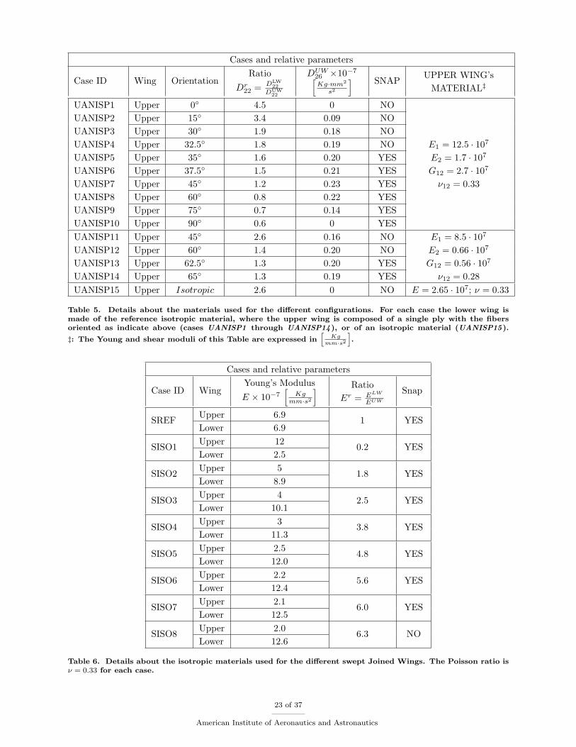
materials are adopted. For these cases the laminates’ thicknesses are kept constant whereas the laminationschemes are changed. Each lamina or ply is identified by a material coordinate system which is in generalnot coincident with the global coordinate system adopted in the solution of the problem. For that reason itis necessary to specify the fibers’ orientation angle at ply level. In this work the angle is measured startingfrom the wing’s local x-axis: in the unswept case it coincides with the global x-axis, see Figure 1, whereasfor the swept case each wing has its own local reference x-axis (xUW and xLW for the upper ad lower wingsrespectively: see Figure 2). The local x-axis is always perpendicular to the wing span direction and is notparallel to x in the general case of swept Joined Wing. Although in Figure 2 local coordinate systems aredepicted for both the wings, in the swept Joined Wing cases only isotropic materials have been used for thelower wing in the present work.A snapping phenomenon at global structural level (see also Reference [46]) as those that will be discussedhere could not be accepted. It is also true that, when possible, the structures in aeronautical engineering aredesigned pursuing as much as possible a linear response. According to these observations, it may be stated,incorrectly, that a structural analysis may lose of interest well before a limit point is reached.It may be argued that the configurations for which snap occurs are subjected to a deformation which wouldnot be realistic for a joined-wing aircraft.However, the following observations could be made. First, the choice of the dimensions of the baselinemodels (see Figures 1 and 2) have been selected to be consistent with wind-tunnel scaled models. Second,the loads have been accordingly selected to observe the instability phenomenon, in an effort of conceptualunderstanding of the geometric nonlinearities and the effects of composite materials for both swept andunswept configurations.The fundamental aspects of the nonlinearities are necessary to properly design these configurations: JoinedWings present an intrinsic strong geometric nonlinearity even at small angles of attack due to the complexlower wing/joint/upper wing load transferring and stiffening/softening effects which must be properly takeninto account.

8 of 37


It has been observed in literature how complex could be the structural interaction between the wings andthe joint that rise in a joined-wing configuration. Linear analysis may be inadequate, and nonlinearityseems to be inherent.29,46 These effects are tied up with the snap-buckling occurrence and the response is aconsequence of the same physics. Although research has already been carried out on the joined-wing topic,analysis and interpretation of the inherent mechanism responsible for the snap-buckling has only been recentlydiscussed for the case of isotropic [46] structures. Thus, the focus is on the more in depth understandingof the phenomenon and how the adoption of composite materials changes the strongly nonlinear structuralbehavior. Potential benefits of the adoption of composites could be represented by avoiding of snap-bucklingoccurrence and this aspect is extensively assessed in this work. It should be pointed out that the efficientdesign of composite plate-like wings in view of achieving an optimal response (e.g., quasi-linear or snap-buckling-free response) has practical implications since a real wing-box structure could be analyzed with anequivalent plate representation.47 In other words, the analyses reported in this work could be adopted togain directions about the design of a real snap-free joined-wing structure.Under the logic of understanding the physics related to the highly complex critical and post-critical behaviorof composite anisotropic Joined Wings, the material properties used in the investigations are artificiallymodified to gain insights on the actual structural parameters which affect the structural response.

IV. Unswept Joined Wing Cases

The unswept cases present the geometry shown in Figure 1 whereas the material properties are case-by-case changed to identify the important parameters affecting the nonlinear response. The joint transfers forcesand moments between the wings. Thus, it is intuitive to expect a significant influence of the extensional andbending stiffness on the nonlinear buckling and post-critical responses. On this regard, if one considers theanalogy with Euler’s column and its instability properties when subjected to compressive forces, it couldbe inferred that when the two wings are loaded with a vertical pressure in the +z direction the consequentcompression of the upper wing is the driving mechanism to the instability. Thus, a design strategy aimed atincreasing the extensional stiffness could be suggested. Actually, in this work a counterintuitive result willbe demonstrated: the bending stiffness is the most relevant parameter which could not be easily predictedby simply using the joined-wing analogue argument of Euler’s column instability. This surprising result isa measure of the complex interaction of the different aspects in the nonlinear response of Joined Wings.Moreover, it will be shown that the bending stiffness ratio between the lower and upper wings is whatregulates the nonlinear buckling for the unswept configuration reported in Figure 1.

It was also observed that for this unswept layout the cases undergoing nonlinear buckling deform, afterthe first limit point (i.e., the state at which the tangent stiffness matrix is singular) is reached, in such a waythat the upper and lower wings tend to interpenetrate.46 This happens starting from a state in the unstablebranch, which lies between the first limit point (representing the end of the stable branch and the transitionto the unstable one) the second limit point (representing the end of the unstable branch and the transitionto another stable branch). Further tracking the load-displacement curve, this interpenetration continues toexist and persists in the post-critical stable branch. All the states presenting interpenetration are obviouslynot physical. However, this does not affect the validity of the drawn conclusion. Global scale snap-bucklingoccurrence is not accepted a-priori regardless of the existence or not of the post buckled configuration inpractice.

A. Lower-to-Upper Wing Stiffness Ratio and its Effects on the Snap-buckling

The isotropic, orthotropic and anisotropic cases are now investigated.

1. Isotropic case

To gain physical insight on the highly complex and nonlinear response of the Joined Wing, the Young’smoduli are varied. The moduli are freely selected to change the lower-to-upper wing stiffness ratio, but theconstraint represented by UREF configuration’s linear vertical displacement of the lower wing’s tip (seepoint P1 in Figure 1) is adopted for a meaningful comparison. In the process of varying the material ofthe wings (see Table 1), the joint’s material has been held the same. The results of these investigationsare shown in Figures 3 and 4. For details on each of the configurations, refer to Table 1. All the anal-

9 of 37


Figure 3. Load parameter Λ versus cumulative vertical displacement Uz of lower wing’s tip point P1 forconfigurations employing different isotropic materials (UISO1 to UISO5). See Table 1 for details.

Figure 4. Load parameter Λ versus cumulative vertical displacement Uz of lower wing’s tip point P1 forconfigurations employing different isotropic materials (UISO6 to UISO10). See Table 1 for details.

yses with the present software have been validated with NASTRAN, and the agreement has proven to beexcellent, although in many cases it was not possible to drive to convergence the commercial tool after thelimit point, showing the difficulties of this type of simulations for the case of Joined Wings and the utility ofthe automatic switching features (from Newton-Raphson to arc length and vice-versa) implemented in thein-house capability. From Figures 3 and 4 it can be inferred that the responses almost coincide before snapphenomena occur. This is a consequence of the choice of the elastic moduli selected with the condition tohave for all the cases the same linear displacement as the one corresponding to the UREF configuration.

It can also be observed that the lower-to-upper wing stiffness ratio Er = ELW

EUW plays an important role indetermining the nonlinear response and snap phenomenon occurrence. From Figure 3 it can be inferred thatincreasing Er raises the nonlinear buckling load level (i.e., the first limit point encountered when tracking theresponse curve occurs at higher values of Λ). Further increasing (Figure 4) of the stiffness ratio Er postponesthe buckling occurrence to higher level loads, and eventually it disappears (see the curve corresponding tothe UISO10 configuration which has Er = 2.5) and the response presents a stiffening effect (increasing ofthe load parameter/displacement slope).From the definition of Er it is also deduced that increasing the stiffness of the lower wing compared to thestiffness of the upper wing is beneficial as far as the elimination of the nonlinear buckling is concerned. This

10 of 37


Cases and relative parameters

Case ID WingYoung’s Modulus

E × 10−7[

Kgmm·s2

] Ratio

Er = ELW

EUW

Snap

UREFUpper 6.9

Lower 6.91 YES

UISO1Upper 12

Lower 2.40.2 YES

UISO2Upper 10

Lower 4.10.4 YES

UISO3Upper 8.7

Lower 5.20.6 YES

UISO4Upper 7.7

Lower 6.10.8 YES

UISO5Upper 6.0

Lower 7.81.3 YES

UISO6Upper 5.0

Lower 8.91.8 YES

UISO7Upper 4.5

Lower 9.52.1 YES

UISO8Upper 4.1

Lower 9.92.4 YES

UISO9Upper 4.1

Lower 102.45 YES

UISO10Upper 4.0

Lower 10.12.5 NO

Table 1. Details about the materials used for the different configurations. Poisson’s ratio is ν = 0.33 for allcases.

is apparently a counterintuitive result since it would be expected that increasing the stiffness of the upperwing (the one which is compressed under this load condition) is beneficial. It also confirms the fact that forJoined Wings the type of response does not follow the interpretation which could be used by adopting theclassical arguments of the Eulerian compressed column.Figure 5 shows the comparison (for Λ = 0.9) of the deformed shapes for two different configurations whichpresent different stiffness ratios Er. In particular, the UREF (which does experience buckling) and UISO10(which does not present buckling) configurations are selected. It can be inferred that while the deformationsof the lower wing is quite similar for both cases, the deformations of the upper wing is very different. More-over, the configuration UREF which is on the verge of snapping (for that load level) presents a deformation ofthe upper wing characterized by a more pronounced inward bending deformation, as it could be observed inFigure 5. It is surprising that the two configurations, presenting remarkably different shapes, carry the sameloads and show comparable global stiffness. A little increment in the load enhances the different deformationmodes, until, for the UREF case, snap occurs.

Summarizing, to avoid snap-buckling and having on the contrary a stiffening effect, the ratio Er seems tobe one of the dominant parameters. In particular, a configuration featuring a value of this parameter largerthan a critical value Er

CR, does not present a snap-buckling problem. A stiffer lower wing (or alternativelya more compliant upper wing) is then desirable for avoiding the snap-buckling problem. The differentstiffness of the two wings also implies a difference share of the load carried by each wing. This also presentsimplications on the stress levels reached by the structure and has to be properly taken into account whenthis type of configurations are designed.

11 of 37


Figure 5. Comparison of configurations UREF and UISO10 (featuring Er = 1 and Er = 2.5 respectively) atΛ = 0.9. Both a tridimensional and a side view are shown.

2. Orthotropic case

In the analysis of Joined Wings made of isotropic materials it was observed (see for example Figure 5) thatthe bending deformation is strictly tied with the snap-buckling occurrence. It should also be observed thatan isotropic material does not present a preferential direction and, thus, the nature of the nonlinear responsecan be fully investigated only if anistotropic materials are adopted. As a first step towards this direction,the case of orthotropic plates is here analyzed.The first test case involves a single lamina with fibers directed along the wing span. That is it: the fibers’angle ϑ, measured counterclockwise from the x-axis is equal to 90 degrees. This choice makes the materialbehavior to be orthotropic in respect of the free stream x and span-wise y directions. The investigations arecarried out by changing the values of E1 and E2 (elastic moduli in the y and x directions respectively). Asdone for the previously discussed isotropic case, the simulations are performed by selecting the values of thematerial properties which make the linear static response of point P1 identical to a reference value. Thisreference value was chosen by a formal substitution of the elastic moduli EUW

1 and ELW1 (elastic moduli in

the fibers’ direction for the upper and lower wings respectively) in the analytical formula calculated with alinear beam theory for the case of isotropic upper and lower wings. This means that the reference value isno longer the true linear displacement of point P1 but it has only a normalization value to restrict the spaceof analyzed displacement curves.The following assumptions are made:

• ELW2 = EUW

2 = EREF, GLW12 = GUW

12 = GREF, and νLW12 = νUW12 = νREF are set. The values of ELW

1 andEUW

1 are freely varied with the only constraint represented by the prescribed initial slope (referencesolution) calculated as described above.

• The joint’s material is fixed and is exactly the isotropic one used for the baseline case, UREF.

Results of the analysis are depicted in Figure 6, where the details of each case are shown in Table 2. It isevident that the ratio Er

1 , although significantly affecting the response, is not reproducing the same resultsas for the isotropic case (see effects of Er previously discussed). To support this, it is enough to comparethe response of the cases UORTHO3 (for which Er

1 = 2.5) and UISO10 (for which Er1 = Er = 2.5). The

curves corresponding to these two cases are reported in Figures 6 and 4 respectively. Having both of theconfigurations a value of the stiffness ratio Er

1 equal to 2.5, according to conclusions relative to the isotropiccase previously discussed, they both should not incur in buckling. However, this is not the case, since theorthotropic configuration UORTHO3 presents a snap. It is then realized that the parameter Er

1 is not a goodbuckling predictor for non-isotropic materials (given the unswept Joined Wing configuration). Summarizing,

12 of 37


Figure 6. Load parameter Λ versus cumulative vertical displacement Uz of point P1 for configurations employingdifferent orthotropic wings. See Table 2 for details.



E1 × 10−7[

Kgmm·s2

] Ratio

Er1 =

ELW1

EUW1

Ratio

Ar22 = Dr

22 =DLW

22

DUW22

Snap

UORTHO1Upper 5.0

Lower 8.91.8 1.7 YES

UORTHO2Upper 4.5

Lower 9.52.1 1.9 YES

UORTHO3Upper 4.0

Lower 10.12.5 2.2 YES

UORTHO4Upper 3.7

Lower 10.42.8 2.4 YES

UORTHO5Upper 3.4

Lower 10.83.2 2.7 NO

Table 2. Details about the materials used for the different configurations. For each case it holds that E2 = EREF,ν = νREF, G = GREF.

in the case of isotropic materials it has been shown (see previous discussions) that Er = Er1 was the most

important parameter to qualitatively predict the nonlinear response. In the case of orthotropic materialsthis is not the case. Understanding the physical reason could explain the mechanism driving the snapphenomenon.An explanation could be attempted as follows. Since the upper and lower wings have uniform thickness (inthe examined case it is hUW = hLW = h), it is possible to identify the ALW, AUW, DLW and DLW matricesas being representative of the whole wings’ stiffness and determining thus their behavior. The superscriptspecifies the wing which the A and D matrices are referring to. Since the material is orthotropic, it can be

13 of 37


inferred, for example for the upper wing (note that the fibers are oriented along the span),

AUW = hUW

EUW

2

1− νUW12 νUW

21

νUW12 EUW

2

1− νUW12 νUW

21

0

νUW12 EUW

2

1− νUW12 νUW

21

EUW1

1− νUW12 νUW

21

0

0 0 GUW12

(25)

DUW =

(hUW

)312

EUW

2

1− νUW12 νUW

21

νUW12 EUW

2

1− νUW12 νUW

21

0

νUW12 EUW

2

1− νUW12 νUW

21

EUW1

1− νUW12 νUW

21

0

0 0 GUW12

(26)

Similar equations could be written for the lower wing.The idea is to monitor the terms of the matrices Ar

mn and Drmn which contain the ratios of the corresponding

terms for the upper and lower wings:

Armn =

ALWmn

AUWmn

Drmn =

DLWmn

DUWmn

(27)

where m and n are indexes identifying each non-zero term of the corresponding matrix.Since each term of these matrices has a direct physical meaning, it is possible to find a parameter which

strictly correlates with buckling. This is accomplished as follows. First it is observed that each wing isanalyzed with a single lamina with constant thickness and material properties. This means that the matrixAr which contains the ratios between the extensional stiffnesses is coincident with the matrix Dr whichcontains the ratios of the bending stiffnesses. Second, a series of investigations correlates the snap-bucklingoccurrence with the ratios Ar

22 and Dr22. This is physically expected since Ar

22 relates the extensionalstiffnesses in the wing span direction (important for example to describe the compression or tension of thewings) whereas Dr

22 relates the flexural stiffness (important in the determination of the principal bendingmoment of the wings). Table 2 presents the values of Ar

22 and Dr22 for the analyzed cases. It is immediately

observed that in the single-lamina orthotropic cases (subject of this discussion) it is Ar22 = Dr

22. However, it

is Er1 ≡ ELW

1

EUW1

= Dr22. This can be easily verified from the definitions previously reported:

Dr22 =

DLW22

DUW22

=

ELW1

1−νLW12 νLW

21

EUW1

1−νUW12 νUW

21

=

ELW1

1−νLW12 νLW

12

ELW2

ELW1

EUW1

1−νUW12 νUW

12

EUW2

EUW1

=ELW

1

EUW1

1− νUW12 νUW

12EUW

2

EUW1

1− νLW12 νLW12ELW

2

ELW1

= Er1

1−(νUW12

)2 EUW2

EUW1

1−(νLW12

)2 ELW2

ELW1

(28)

where the relation ν21 = ν12E2

E1has been used to simplify the expressions.

It should be noted that if the upper and lower wings present isotropic materials (Poisson’s ratio is assumedto be the same as previously assumed for the isotropic case) then equation 28 leads to Dr

22 = Er1 . Similar

considerations for the orthotropic and isotropic cases could be adopted for the Ar22 ratio.

Summarizing, results of the isotropic and orthotropic investigations showed that the driving parameterfor the snap-buckling occurrence is the term Dr

22 = Ar22. The deformation trends follow those of the

isotropic cases. Two configurations are depicted in Figure 7, one associated with the case UORTHO1, whichhas Er

1 = 1.8 and Dr22 = Ar

22 = 1.7, and the other one corresponding to the case UORTHO5, featuringEr

1 = 3.2 and Dr22 = Ar

22 = 2.7. The first case is incurring in a snap phenomenon, where the second onedoes not. The configurations deform accordingly with what already seen: although tip displacements arepractically identical, the configuration UORTHO1 is close to the non nonlinear buckling condition (limitpoint). Distinctive feature of this configuration is the deformation of the upper wing, which tends to have amore pronounced inward bending.

In the isotropic case it was shown that the driving parameter for which the snap-buckling occurs wasthe stiffness ratio Er and, for the analyzed geometry, the snap-buckling disappeared if Er was larger than a

14 of 37


Figure 7. Comparison of configurations UORTHO1 and UORTHO5 at Λ = 1.

critical value ErCR (∼ 2.5). By selecting each wing to be a single orthotropic lamina, it was discovered that

the actual driving parameters are the ratios Ar22 and Dr

22. The snap-buckling disappeared (for the samegeometry of the Joined Wing) when Ar

22 = Dr22 > Er

CR. However, it was not clear the relative importanceof Ar

22 and Dr22 since for the single orthotropic lamina these two parameters are identical. The knowledge of

the relative importance is crucial in the design of a Joined Wing. For example, if Ar22 is the most important

term then the nonlinear buckling occurs mainly because of the compressive actions. On the other hand,if Dr

22 is the most important parameter then the snap-buckling occurs mainly because of bending actions.If the two parameters have similar relative importance, the physical mechanism is a combination of bothcompression and bending. To resolve this crucial theoretical dilemma, a larger-than-one number of plies isselected so that it is possible to separately modify Ar and Dr matrices with the important consequence thatAr = Dr. In particular, several test cases have been introduced with the following assumptions:

• The lower wing is made of the same isotropic material employed for the reference case.

• The upper wing is made of a multilayered orthotropic composite laminate with layers made of the samematerial.

• The thickness of two generic different layers may be different, but the total thickness of the upper wingis maintained equal to h = 1mm.

Table 3 shows all the analyzed cases and the values of Ar22 and Dr

22 for each configuration. For these casesa reference closed-form analytical linear solution is impractical to obtain. Thus, it is not imposed to havethe same slope (linear solution) for all the nonlinear responses relative to the cases reported in Table 3. Onthe other hand, to restrain the design space, the lower wing has been maintained composed of the samematerial, the reference material. Simulations have demonstrated that the value of the Er

CR for such a choiceis not appreciably different from the previous one, having now a value of 2.6. That said, the investigationcould carry on to reach the understanding of the relative importance between Ar

22 and Dr22.

Figures 8 and 9 summarize the responses of all the performed analyses. It is quite evident that Dr22 plays

the leading role, since it dictates snap occurrence, where this is shown to be quite insensitive to the Ar22

factor. For example (see Table 3), when Ar22 is held constant and equal to 1.7 and Dr

22 is increased from 1.0to 2.9, the snap-buckling disappears. Similar considerations, leading to the same conclusions, could be donefor the other entries of Ar

22 and Dr22 reported in Table 3. The importance of the ratio Dr

22 is qualitativelyconsistent with the previous finding which showed that when the nonlinear buckling occurs a significantinward bending deformation of the upper wing is present.

15 of 37



Case ID Wing LaminationRatio

Ar22 =

ALW22

AUW22

Ratio

Dr22 =

DLW22

DUW22

SNAP

UORTHOMP1 Upper 900.15/00.7/900.15 2.5 1.3 YES

UORTHOMP2 Upper 900.1/00.35/900.1/00.35/900.1 2.5 1.7 YES

UORTHOMP3 Upper 900.05/00.35/900.2/00.35/900.05 2.5 2.7 NO








Table 3. Details about the materials used for the different configurations. For each case the lower wing is madeof an isotropic material with ELW = EREF, νLW = νREF, where the upper wing features a composite material

with plies laminated as indicate above. Each ply is manufactured with the same material E1 = 8.5 · 107[

Kgmm·s2

],

E2 = 0.66 · 107[

Kgmm·s2

], G12 = 0.56 · 107

[Kg

mm·s2

], ν12 = 0.28.

Figure 8. Load parameter Λ versus cumulative vertical displacement Uz of point P1 for configurations featuringa lower wing composed of reference isotropic material (E = EREF and ν = νREF) and an upper wing composed ofmulti-ply composite material in order to have an orthotropic response. The different laminations are indicatedin Table 3.

3. Joint’s Connection and Load Transferring Effects on the Snap-Buckling of Unswept Joined Wings

For both the cases of orthotropic and isotropic unswept Joined Wings, configurations which showed similartip displacement for the same load level Λ but different nonlinear behavior (i.e. one configuration experiencedsnap-buckling and the other did not, see for example Figure 5) were compared. One of the main features thatwas noticed was the different deformation of the upper wing. In particular, the curvature was significantlydifferent for the model that was on the verge of snapping. It is true that the curvature distribution of theupper wing depends on all the transmitted force through the joint, being this exacerbated from the large

16 of 37


Figure 9. Load parameter Λ versus cumulative vertical displacement Uz of point P1 for configurations featuringa lower wing composed of reference isotropic material (E = EREF and ν = νREF) and an upper wing composed ofmulti-ply composite material in order to have an orthotropic response. The different laminations are indicatedin Table 3.

displacement characteristic of the cases. However, it is of particular interest to monitor the bending momentMyy transmitted through the joint as a function of the load parameter Λ. In particular, this is done forthe configuration which is on the verge of snapping and for the configuration (presenting different materialproperties than the first one but with similar load-displacement curve up to that load level) which does notpresent nonlinear buckling. Figure 10 shows the moment Myy on a finite element on the upper wing and nearthe joint. The chosen configurations are UISO7 (which presents snap-buckling) and UISO10 (which does

Figure 10. Wing span forces (NUWyy and NLW

yy ) per unit of length and primary bending moments (MUWyy and

MLWyy ) per unit of length transferred to the upper and lower wings. The forces and moments are calculated at

the centroid of the finite elements shown in the figure.

not present snap-buckling). Although the interest is towards trends more than values, to have more reliablepredictions a refined model using approximately 15000 DOF (against the approximately 2600 DOF of the

17 of 37


0 50 100 150 200 250 300 350 4000

0.2

0.4

0.6

0.8

1

1.2

1.4

1.6

1.8

2

UISO7 (in-house FEM, 2670)NDOF=

UISO7 (NASTRAN, 15342)NDOF=


L

Uz [ ]mm

0 50 100 150 200 250 300 350 4000

0.2

0.4

0.6

0.8

1

1.2

1.4

1.6

1.8

2

UISO10 (in-house FEM, 2670)NDOF=



L

Uz [ ]mm

Figure 11. Curves of the load parameter Λ versus cumulative vertical displacement Uz of point P1 for UISO7(onthe left) and UISO10(on the right) obtained from simulations using different FE solvers and mesh sizes. BothNASTRAN solutions showed convergence problems after the first limit point.

base model), is used for comparison purposes. These models show an almost perfect agreement in terms ofcumulative vertical displacement of point P1, see Figure 11. As it is well known, the force and moments (seeFigures 12 to 14) converge more slowly when the mesh is refined. The correlation of their trends is verygood. It should also pointed out that since the forces and moments per unit of length are evaluated at thecentroid of of the elements (see Figure 10 for the base model) a refining of the mesh implies a calculation ofthese quantities on a different (but close) point. The interest of this discussion is to show the trends. Thus,this fact does not affect the following discussion. In Figure 12 and 13 the value of Myy is plotted for boththe upper and lower wings for both the cases. Considering the upper wing, it is possible to observe thatMUW

yy shows similar trend in the pre-buckling area. However, the configuration which does not experience

snap-buckling (UISO10 ) presents a larger moment MUWyy compared to the one corresponding to UISO7. At

a certain load parameter, smaller than the critical value, the moment relative to configuration UISO7 startsdiminishing in value and eventually the snap-buckling occurs. For the lower wing the bending moments ofthe UISO7 and UISO10 configurations are practically identical. For completeness, Figure 14 shows theforce per unit of length Nyy on the upper wing (see also Figure 10).The different trends regarding the transmitted bending moment (see Figure 12) suggest that the snap-buckling occurrence could be strictly tied with Myy. To further demonstrate this observation, the boundaryconditions between the joint and the upper wings are now modified to reduce the amount of moment whichis transferred. This is accomplished by the adoption of a multifreedom constraint which allows the joint-upper-wing relative rotation. To simulate some stiffness of the joint a relatively small torsional spring

(kϑ = 100Kg·mm2

s2·rad ) has also been added at the joint-upper-wing connection. It should be noted that a largevalue for the spring stiffness would correspond to a perfect joint’s connection of the types analyzed so far,whereas a zero-value for the stiffness of the spring would correspond to a perfect hinge connection. Sincethe adopted value for the torsional stiffness is quite small compared to the stiffness of the finite elements,the simulated joint-upper-wing connection is similar (but not equivalent) to a hinge connection. This set ofboundary conditions is referred as quasi-hinge connection in this work.A quasi-hinge connection reduces the amount of moment transferred by the joint to the upper wing. Thus,it is expected that the nonlinear response is improved. In other words, it is expected that this connectionhas the tendency to reduce or eliminate the nonlinear buckling occurrence. To prove that, two configu-rations which both experience the snap-buckling instability are considered. In particular, the UREF andUISO7 configurations are investigated. The quasi-hinge connection is adopted and the consequent nonlinearresponses are plotted in Figure 15. It can be observed that the snap-buckling disappears in both cases asexpected. It can inferred from Figure 15 that avoiding the bending moment transmission prevents the snapto occur. Moreover, if the responses relative to the quasi-hinge connection are superimposed to the perfect-joint ones, Figures 3 and 4, it is possible to realize that the configurations featuring a quasi-hinge connectionexperience a loss of stiffness, at least before the snap occurs. This loss in stiffness seems to be more relevant

18 of 37


Figure 12. Bending moment per unit of length Myy on the upper wing for the UISO7 and UISO10 cases. Seealso Figure 10 for a graphical representation.

when the two wings have Young’s moduli relatively similar (for the case of UREF configuration the elasticmoduli are exactly the same). Summarizing, the carried out analyses lead to the conclusion that bendingeffects are one of the main sources of non-linearities when stability is concerned.

4. Composite Materials (anisotropic case)

Previous discussions showed that for the isotropic and orthotropic cases the driving mechanism which leadsto the snap-buckling is closely tied with bending effects. It was also demonstrated that the bending stiffnessratio Dr

22 was an effective parameter to predict if the nonlinear response presents a snap-buckling instability.In particular, it was shown that the upper wing has to be more bending compliant to avoid the snap-buckling.

It was found that when Dr22 ≡ DLW

22

DUW22

is bigger than a critical value, then the instability disappears. Moreover,

[Dr22]CR does not represent an universal value: its magnitude is a case-dependent parameter.

For the same unswept joined-wing layout, the next step is the adoption of composite materials to introduceanisotropy effects and investigate how they influences the nonlinear response. In particular, two mainquestions are here answered:

• Is still the parameter Dr22 sufficient to describe the tendency of the structure to experience a snap-

buckling?

• How does the anisotropy affect the global bending stiffness and snap-buckling?

To answer the first question, two new configurations are investigated (see Table 4). In the first one, namedUANIMP1, the lower wing is isotropic and the material is the one adopted for UREF configuration. Theupper wing is simulated with a multilayered orthotropic plate. The second configuration, named UANIMP2,presents a symmetric laminate for the upper wing, whereas the lower wing is made of the same isotropicreference material. In other words, the configurations UANIMP1 and UANIMP2 have identical lower wingswhereas the upper wings are made of different composite structures (see Table 4). Both configurationspresent the same value for Dr

22; however, the nonlinear responses are dramatically different (see Figure 16)and the configuration UANIMP2 does not experience snap-buckling. This qualitative investigation showsthat the new coupling between the torsional deformation and bending moment plays an important role asfar as the stability properties are concerned.

19 of 37


Figure 13. Bending moment per unit of length Myy on the lower wing for the UISO7 and UISO10 cases. Seealso Figure 10 for a graphical representation.

A series of additional configurations have been created (see Table 5). In all configurations reported in Table5 the lower wing is isotropic and the adopted material is the one used for the UREF case. The upperwing is simulated with a single lamina whose orientation is varied according to Table 5. This changes thebending-torsional coupling since the term DUW

26 is not zero for a generic fiber’s orientation angle. Severalinvestigations (see Figures 18 and 19 and Table 5) indicated that the bending-torsional coupling has a majorrole in determining when the snap-buckling occurs. This is clearly understood if for example configurationsUANISP2 and UANISP4 are compared. The two configurations do not present snap-buckling, althoughthis was expected for the first one having Dr

22 > [Dr22]CR(∼ 2.6), if was not expected for the second one,

for which Dr22 < [Dr

22]CR. Analogous situation come when comparing UANISP11 and UANISP12. And,interesting enough, the unexpected behaving cases have a value of DUW

26 different than zero. Since the wingsystem is unswept, the coupling between the torsion and bending are due only to the anisotropy of thematerial. This is why for the anisotropic case understanding the mechanism which leads to the instability ismore challenging. To answer the second question, three different configurations (UISO12, UANISL4 and


Case ID Wing LaminationRatio

Dr22 =

DLW22

DUW22

SNAP

UANIMP1 Upper 900.049/00.25/900.402/00.25/900.049 2.4 YES

UANIMP2 Upper 170.1/450.8/170.1 2.4 NO

Table 4. Details about the materials used for the different configurations. For each case the lower wing iscomposed of the reference isotropic material, where the upper wing is composed of a composite material with

plies laminated as indicate above. Each ply is manufactured with the same material E1 = 8.5 · 107[

Kgmm·s2

],

E2 = 0.66 · 107[

Kgmm·s2

], G12 = 2.6 · 107

[Kg

mm·s2

], ν12 = 0.33.

UANISL12 ) are selected. None of them experiences the nonlinear buckling. Moreover, from the plot of theresponses it can be deduced that all of them have high overall stiffness. The configurations UANISP4 andUANISP12 are even stiffer than the configuration UISO12 (especially for larger values of the load step Λ)

20 of 37


Figure 14. In-plane force per unit of length Nyy on the upper and lower wings for the UISO7 and UISO10cases. See also Figure 10 for a graphical representation.

confirming that composite materials can be effectively used to change the structural behavior of the system.In the practice, the design is more challenging since it must be taken into account the structural weight

and stress levels. Moreover, the actual aerodynamic loads are of a non-conservative type and the torsional-bending coupling is then even more important: the aerodynamic forces are heavily affected by a change ofangle of attack (torsion) of the wing. This study is only the first step in the understanding of the difficultiesand challenges associated with the nonlinear response for the case of anisotropic Joined Wings.

V. Swept Joined Wings and Composites

From the analysis of unswept Joined Wings two main concepts could be identified:

• The ratio between the bending stiffness of the wings is an important parameter to establish if thesnap-buckling occurs. In particular, the upper wing has to be more bending compliant than the lowerwing to remove the instability.

• The anisotropy introduces an artificial coupling between the torsion and bending which is not presentin isotropic unswept Joined Wing. This coupling modifies the snap-buckling occurrence.

A similar study is now attempted for the swept Joined Wings (see Figure 2). It is necessary to investigatethis case since even when isotropic materials are used, a coupling between the bending and torsion dueto the geometry of the wing system arises. It may also be observed (see Figure 2) that the sweep angleis moderately low. It is then reasonable to expect that the snap occurrence is still regulated by bendingstiffness related parameters.

In order to better investigate the physics related to the bending, it is useful to introduce two localcoordinate systems, one for each wing. The direction of the z-axis remains parallel to the global z-axis,whereas the local y-axis runs along the wing-span direction. In such a way the terms of the D matrices forthe upper and lower wings maintain an immediate physical interpretation. Figure 2 clarifies the orientationof the lower and upper wing local axes.

21 of 37


Figure 15. Cumulative vertical displacement (Uz) of point P1 versus load factor (Λ) for UISO7 and UREFconfigurations when a quasi-hinge connection is used between the joint and the upper wing.

A. Effects of Lower-to-Upper-Wing Stiffness Ratio

1. Isotropic case

The ratio of the Young’s moduli of the two wings is varied. However, the selection of the Young’s moduli isselected so that the initial slopes of the displacements are the same (the initial slope is related to the stiffnessof the linear analysis). The details about the materials of each configuration are shown in Table 6, and thegraphs of the cumulative vertical displacement of point P1 are presented in Figures 21 and 22. It can be

inferred that, as in the unswept case, the ratio Er = ELW

EUW has an important role. However, the requiredvalue for avoiding snap is considerably larger (see Table 6) than the one needed for the unswept wings case.This means that the lower wing has to be much stiffer than the upper wing in order to avoid snap-buckling.

It is possible to observe that each wing of the swept configuration results to be a slightly longer andleaner (higher aspect ratio) than the previous unswept cases. However, since the sweep angle is small, theaspect ratio is not significantly affected. The consistent difference of the critical ratio Er found for the sweptcase could be thought to come mainly from effects introduced by the torsion.

Analyses of two configurations, one incurring in snap, SISO5, and one not, SISO8, for two different loadconditions are depicted in Figures 23 and 24. For the load level Λ = 0.5 SISO5 is not very far to buckle,however, the two deformed shapes are almost superimposed, except for the upper wings. In the ISO5 case,upper wing experiences a bending deformation which points inward. This is similar of what was found inthe unswept cases.

The load level Λ = 0.6 represents a post-buckling situation for the configuration SISO5, as it could beverified in Figure 22. Besides experiencing an almost rigid rotation along x−axis, in this case the jointundergoes a negative rotation along global y-axis as well.

In conclusion, it can be stated that the interactions between the wings are more complicated in the caseof swept Joined Wings even when isotropic materials are used. This is due to the rise of forces inherent to thegeometrical layout which couples the bending and torsional effects. These forces have an important role ininfluencing the snap phenomenon: although the span-wise bending actions drive the instability phenomenon,torsion contributes to regulate it. For example, compared to the unswept isotropic cases, the lower wing has

22 of 37



Case ID Wing OrientationRatio

Dr22 =

DLW22

DUW22

DUW26 ×10−7[Kg·mm2

s2

] SNAPUPPER WING’s

MATERIAL‡

UANISP1 Upper 0◦ 4.5 0 NO

UANISP2 Upper 15◦ 3.4 0.09 NO


UANISP4 Upper 32.5◦ 1.8 0.19 NO

UANISP5 Upper 35◦ 1.6 0.20 YES

UANISP6 Upper 37.5◦ 1.5 0.21 YES




UANISP10 Upper 90◦ 0.6 0 YES

E1 = 12.5 · 107

E2 = 1.7 · 107

G12 = 2.7 · 107

ν12 = 0.33



UANISP13 Upper 62.5◦ 1.3 0.20 YES


E1 = 8.5 · 107

E2 = 0.66 · 107

G12 = 0.56 · 107

ν12 = 0.28

UANISP15 Upper Isotropic 2.6 0 NO E = 2.65 · 107; ν = 0.33

Table 5. Details about the materials used for the different configurations. For each case the lower wing ismade of the reference isotropic material, where the upper wing is composed of a single ply with the fibersoriented as indicate above (cases UANISP1 through UANISP14), or of an isotropic material (UANISP15).

‡: The Young and shear moduli of this Table are expressed in[

Kgmm·s2

].



E × 10−7[

Kgmm·s2

] Ratio

Er = ELW

EUW

Snap

SREFUpper 6.9

Lower 6.91 YES

SISO1Upper 12

Lower 2.50.2 YES

SISO2Upper 5

Lower 8.91.8 YES

SISO3Upper 4

Lower 10.12.5 YES

SISO4Upper 3

Lower 11.33.8 YES

SISO5Upper 2.5

Lower 12.04.8 YES

SISO6Upper 2.2

Lower 12.45.6 YES

SISO7Upper 2.1

Lower 12.56.0 YES

SISO8Upper 2.0

Lower 12.66.3 NO

Table 6. Details about the isotropic materials used for the different swept Joined Wings. The Poisson ratio isν = 0.33 for each case.

23 of 37


Figure 16. Cumulative vertical displacement of P1 versus Λ for two different configurations featuring a lowerwing composed of an isotropic material and an upper wing with an orthotropic and anisotropic behavingmaterials, obtained through a different disposition of plies. As a consequence of the ad-hoc lamination schemesof the plies, the ratio Dr

22 is equal for the two cases. See Table 4 for details.

Figure 17. Comparison of the deformed configurations for configurations UANIMP1 and UANIMP2. Noticehow in the anisotropic torsion deformation are introduced, leading to a lateral tilting of the joint.

to be significantly stiffer in order snap to be avoided. This could be intuitively explained as follows. Figure24 shows that when the instability takes place a significant rigid rotation of the joint is experienced. Thus,the high stiffness is “required” to counteract also this joint’s rotation and thus, the snap-buckling is avoided.

2. Anisotropic Effects

For this study, the lower wing is assumed to be made of the same isotropic material used for the UREF con-figuration. However, the upper wing is now composed of a single lamina. The fiber’s orientation is measuredstarting from the upper wing local axis xUW, as depicted in Figure 2. Table 7 reports the configurations

24 of 37


0 100 200 300 4000

0.2

0.6

1

0 100 200 300 4000

0.2

0.6

1

0 100 200 300 400

0.2

0.6

1

Uz [ ]mm

L L L

UANISP3

UANISP2

UANISP1

UANISP7

UANISP6

UANISP4

UANISP10

UANISP9

UANISP8

Uz [ ]mm Uz [ ]mm

Figure 18. Responses for different configurations. The lower wing is composed of the reference isotropicmaterial (E = EREF and ν = νREF) for all the cases, the upper wing is composed of a single layer with

EUW1 = 12.5 · 107

[Kg

mm·s2

], EUW

2 = 1.7 · 107[

Kgmm·s2

], GUW

12 = 2.7 · 107[

Kgmm·s2

]and νUW

12 = 0.33. The orientation of

the fibers for each case is specified in Table 5.

Figure 19. Responses for different configurations. The lower wing is composed of the reference isotropicmaterial (E = EREF and ν = νREF for all the cases, the upper wing is composed of a single layer with

EUW1 = 8.5 · 107

[kg

mm·s2

], EUW

2 = 0.66 · 107[

kgmm·s2

], GUW

12 = 0.56 · 107[

kgmm·s2

]and νUW

12 = 0.28. The orientation of

the fibers for each case is specified in Table 5.

used to assess the anisotropic effects for the swept Joined Wing. It may be inferred that the influence oftorsion is now of primary importance. In fact, some configurations featuring a relatively small value of Dr

22

do not present any snap-buckling phenomenon. It is relevant to investigate the effect of the sign for DUW26

for practically unchanged Dr22 parameters. For example, configuration SANISP16 (for which Dr

22 = 1.39

and DUW26 = −0.20

[Kg·mm2

s2

]) does not experience buckling whereas configuration SANISP6 (for which

Dr22 = 1.30 and DUW

26 = +0.20[Kg·mm2

s2

]) does experience instability.

Not all of the configurations reported in Table 7 experience nonlinear buckling. It is then of a practicalimportance identify the conditions for which buckling occurs from a graphical point of view. This is whatFigure 25 achieves. In particular, the so called Snap Buckling Region SBR for Joined Wings46 can be seenin Figure 25. It should be noted that SBR is actually the union of two subregions which do not presentsymmetry with respect to the zero angle. This is expected since the Joined Wing and its materials do notpresent symmetries and the complex bending-torsion coupling affects the nonlinear response in a non-trivialmanner.Figures 26, 27, and 28 show the responses relative to some of the cases reported in Table 7.

25 of 37


Figure 20. Comparison of responses for configurations UANISP4, UANISP12 and UANISP15. All the threeconfigurations have a lower wing composed of the isotropic reference material. Configuration UANISP15features an upper wing of a different isotropic material, where UANISP4 and UANISP12 have an upper wingcomposed of a single ply composite of two different materials. Details about the materials are reported in Table5. Given the materials, the three configurations represent the stiffer responses which do not show buckling.

Figure 21. Load parameter Λ versus cumulative vertical displacement Uz of lower wing’s tip point P1 forconfigurations employing different isotropic materials (see Table 6).

26 of 37


Figure 22. Load parameter Λ versus cumulative vertical displacement Uz of lower wing’s tip point P1 for con-figurations employing different isotropic materials chosen such that the ratio of Young’s Modulus of the upperwing to the one of the lower wing is varied but the initial rate of change of cumulative vertical displacementof P1 is constant.

Figure 23. Comparison of deformed configurations SISO5 and SISO8 at Λ = 0.5. Tridimensional and side view.

27 of 37


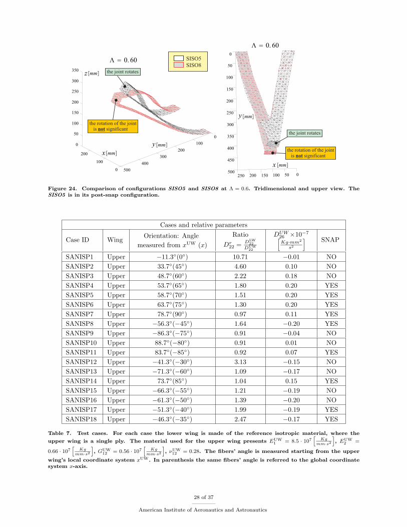
Figure 24. Comparison of configurations SISO5 and SISO8 at Λ = 0.6. Tridimensional and upper view. TheSISO5 is in its post-snap configuration.


Case ID WingOrientation: Angle

measured from xUW (x)

Ratio

Dr22 =

DLW22

DUW22

DUW26 ×10−7[Kg·mm2

s2

] SNAP

SANISP1 Upper −11.3◦(0◦) 10.71 −0.01 NO

SANISP2 Upper 33.7◦(45◦) 4.60 0.10 NO

SANISP3 Upper 48.7◦(60◦) 2.22 0.18 NO

SANISP4 Upper 53.7◦(65◦) 1.80 0.20 YES

SANISP5 Upper 58.7◦(70◦) 1.51 0.20 YES

SANISP6 Upper 63.7◦(75◦) 1.30 0.20 YES

SANISP7 Upper 78.7◦(90◦) 0.97 0.11 YES

SANISP8 Upper −56.3◦(−45◦) 1.64 −0.20 YES

SANISP9 Upper −86.3◦(−75◦) 0.91 −0.04 NO

SANISP10 Upper 88.7◦(−80◦) 0.91 0.01 NO

SANISP11 Upper 83.7◦(−85◦) 0.92 0.07 YES

SANISP12 Upper −41.3◦(−30◦) 3.13 −0.15 NO

SANISP13 Upper −71.3◦(−60◦) 1.09 −0.17 NO

SANISP14 Upper 73.7◦(85◦) 1.04 0.15 YES

SANISP15 Upper −66.3◦(−55◦) 1.21 −0.19 NO

SANISP16 Upper −61.3◦(−50◦) 1.39 −0.20 NO

SANISP17 Upper −51.3◦(−40◦) 1.99 −0.19 YES

SANISP18 Upper −46.3◦(−35◦) 2.47 −0.17 YES

Table 7. Test cases. For each case the lower wing is made of the reference isotropic material, where the

upper wing is a single ply. The material used for the upper wing presents EUW1 = 8.5 · 107

[Kg

mm·s2

], EUW

2 =

0.66 · 107[

Kgmm·s2

], GUW

12 = 0.56 · 107[

Kgmm·s2

], νUW

12 = 0.28. The fibers’ angle is measured starting from the upper

wing’s local coordinate system xUW. In parenthesis the same fibers’ angle is referred to the global coordinatesystem x-axis.

28 of 37


Figure 25. Snap Buckling Region for configurations with different orientation of the upper wing’s fibers (theangles are measured in the upper wing’s local coordinate system). The configurations in the SBR experiencebuckling.

Figure 26. Cumulative vertical displacement (Uz) of point P1 versus load parameter (Λ) for swept JoinedWings featuring different single-layer upper wing. See Table 7 for details.

29 of 37




30 of 37


B. Effects of Composite Materials on Snap Buckling Region

In Reference [46] the so called Snap Buckling Region(SBR) was defined for the SREF configuration (seeTable 6 and Figure 29). In particular, the joint’s height was varied with all the other geometric and material

Point P1

Uz [ ]mm

0 50 100 150 200 250 300 350 4000

0.2

0.4

0.6

0.8

1

1.2

LLSBR

ULSBR a50

69b =

a50

7b =

Snap Buck

ling R

egio

n (SBR)

L

Figure 29. SBR for the SREF based configuration, from Reference [46]. b is the joint’s height.

parameters held constant. Some values of the height led to a nonlinear buckling instability, whereas othervalues did not. The SBR region was identified in the displacement-load parameter plane. Two configu-rations were identified: the Upper Limit Snap-Buckling Region(ULSBR) and Lower Limit Snap-BucklingRegion(LLSBR). SBR has the following property: for each configuration featuring a joint’s height in theSBR, snap-buckling will occur.

However, the study of reference [46] investigated the case of the reference isotropic material only. Thisstudy is now extended to include the effects of composite materials. The goal is to understand how theSBR is affected. It is clear that composites introduce some couplings (e.g. bending-torsion coupling) whichare independent of the ones relative to the geometry (e.g., a swept Joined Wing is significantly differentthan an unswept one). Thus, it is expected to find configuration-dependent SBRs. To explore this fact,two configurations (SANISP4 and SANISP11, see also Table 7) were investigated. The results are reportedbelow.

1. SBR for SANISP4 configuration

The cumulative displacement of point P1 for this case is depicted in Figure 30. According to Table 7 , thefibers are oriented with a 53.7◦ angle measured from xUW (65◦ if the angle is measured from the globalx-axis). The SBR is delimited by the cases featuring a joint’s height of 5

50a and 6550a respectively. The

response curves in between ULSBR and LLSBR behave following similar patterns. The SBR qualitativelyresembles the one obtained for the complete isotropic case and reported in reference [46] (see also Figure29).

2. SBR for SANISP11 configuration

The cumulative displacement of point P1 for this case is depicted in Figure 31. The fibers are oriented witha 83.7◦ angle measured from xUW (which is equal to −85◦ if the angle is measured from x), see Table 7. TheSBR is delimited by the cases featuring a joint’s height of 10

50a and 5050a respectively. Thus, compared to the

31 of 37


Figure 30. SBR for the SANISP4 based configurations.

Figure 31. SBR for the SANISP11 based configurations.

previous SBR, now the snap-free design space has shrunk. It is possible to observe that the responses whichpresent buckling remain limited by the LLSBR and ULSBR responses as it happened for the isotropic casediscussed in Reference [46] and shown in Figure 29.

32 of 37


VI. Conclusions

Post-buckling investigations of composite PrandtlPlane Joined Wings, with particular focus on the fun-damental physical aspects leading to the instability and nonlinear structural response, have been presentedfor the first time.Previous analyses of this promising innovative configuration focused on linear structural and aeroelasticmodels. A first attempt towards an accurate simulation and fundamental understanding of the critical andpost-critical conditions has been presented in Part I (see Reference [46]) where the case of isotropic materialswas discussed. The effects of the geometrical parameters (joint’s dimensions and sweep angles) showed avery complex nonlinear response which could not be predicted with the standard linear analysis but needsto be properly taken into account even in the very early stages of the design. This is particularly importantsince the true nonlinear buckling load can often be over predicted when a classical linear eigenvalue approach(linear buckling analysis) is adopted. Reference [46] showed that increasing the joint’s height is beneficial.Moreover, it can be identified an interval of joint’s heights in which the snap-buckling instability occurs.This was defined as Snap-Buckling Region (SBR). SBR presents a high importance in the conceptual designof PrandtlPlane configurations, since a snap-buckling type of instability must be avoided.Reference [46] also showed that the torsional-bending coupling consequence of the geometric layout (sweptwings) can dramatically worsen the stability properties. Finally, it was also presented that the load repar-tition between the upper and lower wings has a significant effect on the nonlinear response. In particular,for the common PrandtlPlane layout featuring a swept-back lower wing and a swept-forward upper wing, ahigher percentage of the load on the upper wing was showed reducing the risks of buckling.However, several conceptual and theoretical aspects needed to be addressed. This was accomplished in thepresent work. In particular, the effect of anisotropy was extensively investigated by the adoption of compos-ite materials. The following analyses have been carried out.

• Unswept Case with Different Isotropic Materials for the Upper and Lower Wings

An unswept joined-wing layout was investigated. Different isotropic materials were selected for theupper and lower wings. The lower-to-upper-wing stiffness ratio showed to be the driving parameter asfar as snap-buckling instability was concerned. In particular, a counterintuitive result was found: themain mechanism which led to the instability (under aerodynamic-like conservative mechanical loads)was not due to the compression. In fact, increasing the stiffness of the upper wing via incrementingthe elastic modulus enhances the extensional stiffness (in theory beneficial because the upper wing iscompressed), but increases the possibility of having nonlinear buckling. From the Eulerian compressedcolumn analogy this is a highly unexpected result. The over constrained nature of the Joined Wing(compared to the classical cantilevered wings) and the non-planar geometry are responsible of thiscomplex behavior.

• Unswept Case and Adoption of Orthotropic Materials

Additional insight on the nature of the nonlinear buckling was gained by the adoption of a single-lamina orthotropic plate for the upper wing. This choice was useful to detect which stiffness ratiowas actually important for the snap-buckling occurrence. It was found that the ratio between theextensional stiffnesses and the ratio between the bending stiffnesses were the primary parametersaffecting the Joined Wing’s instability properties. As for the isotropic case, it was found that the lowerwing’s stiffness should be larger than the upper wing’s one and the counterintuitive nature of the typeof instability was confirmed. However, the single-lamina orthotropic upper wing had the drawback ofpresenting the lower-to-upper-wing extensional stiffness ratio equal to the lower-to-upper-wing bendingstiffness ratio: it was not possible to truly separate the relative importance between the extensionaland bending effects on the instability.This problem was addressed by adopting a multilayered orthotropic laminate for the upper wing. Thiswas very useful since for this case the lower-to-upper-wing extensional stiffness ratio is in generaldifferent than the lower-to-upper-wing bending stiffness ratio. Several investigations showed then thetrue driving mechanism to the instability: the snap-buckling occurrence is mainly sensitive to thelower-to-upper-wing bending stiffness ratio. In particular, it was shown that increasing the lowerwing’s bending stiffness was beneficial, whereas incrementing the upper wing’s bending stiffness had anegative effect on the stability of the Joined Wing.

33 of 37


• Type of Joint’s Connection and its Effects on Snap-Buckling of Unswept Joined Wings

The importance of the bending moment transferring through the joint is one of the leading mechanismsinvolved in the instability. This was demonstrated by modifying the joint-to-upper-wing connection.In particular, a quasi-hinge type of connection was implemented by inserting a hinge at the joint-to-upper-wing junction and a torsional spring opposing the relative rotation between the joint and theupper wing. A small value of the spring stiffness was selected and the bending moment transferred tothe upper wing was reduced compared to the fixed type of joint previously investigated. This provideda great benefit because the snap-buckling was eliminated, thus, confirming the relevant importance ofthe bending moment transferring in the snap occurrence.

• Unswept Case and Adoption of Anisotropic Materials (Composites)

While the lower wing was assumed to be isotropic, the upper wing was simulated first with a multi-layered orthotropic laminate and second with a multilayered anisotropic laminate presenting identicallower-to-upper-wing bending stiffness ratio. The orthotropic case experienced a strong snap-type in-stability, whereas the anisotropic case did not have the instability at all in the range of explored loadlevels and presented a stiffening effect. Considering the fact that the geometry (unswept Joined Wings)does not introduce any bending-torsion coupling whereas the anisotropic laminate does, it was deducedthat the material-induced bending-torsion coupling is important in the nonlinear response.The bending-torsion coupling was further investigated by selecting a single-lamina with fibers gener-ically oriented. The lower-to-upper-wing bending stiffness ratio and the primary bending-torsionaldeformation coupling term D26 was also monitored. The investigation showed that in some cases thebending-torsional coupling is beneficial and in other cases it deteriorates the stability properties of theJoined Wing. A further insight of this coupling and its effects on the instability could be gained fromthe observation of the joint’s rotation with respect to the wing-span direction. This rotation is heavilyaffected by the torsional-bending coupling. In particular, a properly designed laminate could increaseor decrease the rotation of the joint with enhanced or worsened stability properties.

• Swept Case with Different Isotropic Materials for the Upper and Lower Wings

The swept Joined Wing presents a torsional-bending coupling even if the same isotropic material isadopted for both the upper and lower wings. To gain further insight, the upper wing was selectedto be isotropic but with different elastic modulus compared to the lower wing. Several investigationsshowed that to avoid snap-buckling a substantially larger lower-to-upper-wing bending stiffness ratiowas necessary. A direct observation of the deformed shapes confirmed that when this type of instabilityoccurs the rotation (with respect to the wing span axis) of the joint is significant.

• Swept Case and Anisotropy Effects

A physical insight on the highly complex nonlinear response of PrandtlPlane Joined Wings was gainedby the introduction of coupling effects associated with the anisotropy of the material. While the lowerwing was maintained isotropic, the upper wing was simulated with a single-ply generically orientedmaterial. The analyses showed a very complex bending-torsion interaction: even for a relatively simplesingle-ply upper wing there could be identified two distinct and unsymmetrically located regions inwhich the snap-buckling occurs. In other words, the Snap Buckling Region (i.e., range of fiber orien-tation angles for which the system undergoes a snap-buckling instability) is difficult to predict frompure intuitive considerations.

• Joint’s Height Effects in the Case of Anisotropic Swept Joined Wings

For the isotropic case examined in Reference [46] the joint’s height was varied and it was found that anincrease of the height was beneficial. The Snap Buckling Region was also identified for this case andthe representations on the load parameter-displacement plane was presented. A similar investigationhas been carried out in this work with the adoption of composite materials. The goal was to assesshow the composites affect the SBR in the displacement-load parameter plane. It was found out thatthe joint’s height is beneficial even when the composite materials are used.

The investigations presented in this work shed some light on the very complex nonlinear response of JoinedWings. Results showed that the snap-buckling load is quite sensitive to the bending moment transferred by

34 of 37


the joint to the upper wing. Thus, both the type of joint’s connection and bending stiffness of the wingsplay a significant role.When the bending-torsion coupling is introduced because of either the geometry (sweep angles) or thematerial (composites) or both, predicting a priori if the above mentioned effects are beneficial or not is anextremely challenging task. The simulations conducted in this work seem to suggest that the rotation ofthe joint along the wing span axis is an important factor for further gaining insight on instability and itsproperties.Future works focusing on nonlinear effects of Joined Wings will discuss the theoretical challenges and physicalimplications when mechanical non-conservative loadings of a follower type and aerodynamic forces are takeninto account.

VII. Acknowledgements

The authors acknowledges the support by San Diego State University (College of Engineering).

35 of 37


References

1Letcher, J., “V-Wings and Diamond-Ring Wings of Minimum Induced Drag,” Journal of Aircraft , Vol. 8, 1972, pp. 605–607.

2Wolkovitch, J., “The Joined Wing Aircraft: an Overview,” Journal of Aircraft , Vol. 23, 1986.3Lange, R. H. and et alii, “Feasibility Study of the Transonic Biplane Concept for Transport Aircraft Applications,” 1974,

CR–132462, Lockheed–Georgia Company.4Miranda, L. R., “Boxplane Wing and Aircraft,” US Patent 3,834,654, September 1974.5Frediani, A., “Large Dimension Aircraft,” US Patent 5,899,409, 1999.6Frediani, A., “Velivolo Biplano ad Ali Contrapposte,” Italian Patent FI 2003A000043, 19 February 2003.7Frediani, A., “New Large Aircraft,” European Patent EP 0716978B1, 20 March 2002.8Frediani, A., “The Prandtl Wing,” Innovative Configurations and Advanced Concepts for Future Civil Aircraft, VKI

Lecture Series 2005-2006, Von Karman Institute, June 2005.9Frediani, A., Cipolla, V., and Rizzo, E., “The PrandtlPlane configuration: overview on possible applications to civil avi-

ation,” Variational Analysis and Aerospace Engineering II: Mathematical Challenges for Aerospace Design, edited by G. But-tazzo and A. Frediani, Springer, 2012, (In press).

10Ginneken, D. A. J., Voskuijl, M., Van Tooren, M. J. L., and Frediani, A., “Automated Control Surface Design and Sizingfor the Prandtlplane,” Presented at the 51st AIAA/ASME/ASCE/AHS/ASC Structures, Structural Dynamics & MaterialsConference, Orlando, Florida, 12-15 April 2010.

11Livne, E., “Future of Airplane Aeroelasticity,” Journal of Aircraft , Vol. 40, 2003, pp. 1066–1092.12Livne, E. and Weisshaar, T. A., “Aeroelasticity of Nonconventional Airplane Configurations-Past and Future,” Journal

of Aircraft , Vol. 40, 2003, pp. 1047–1065.13Prandtl, L., “Induced Drag of Multiplanes,” Tech. Rep. TN 182, NACA, March 1924.14Scott, M., Enke, A., and Flanagan, J., “SensorCraft Free-Flying Aeroservoelastic Model Design and Fabrication,” Pre-

sented at the 52nd AIAA/ASME/ASCE/AHS/ASC Structures, Structural Dynamics & Materials Conference, Denver, Colorado,4-7 April 2011.

15Heeg, J. and Morelli, E., “Evaluation of Simultaneous-Multisine Excitation of the Joined Wing SensorCraft AeroelasticWind Tunnel Model,” Presented at the 52nd AIAA/ASME/ASCE/AHS/ASC Structures, Structural Dynamics & MaterialsConference, Denver, Colorado, 4-7 April 2011.

16Chiavacci, L., Progetto Aerodinamico Preliminare di un Velivolo Ultraleggero tipo PrandtlPlane, Ms thesis, Universit diPisa, 2006, Advisors: Prof Frediani A., Prof. Casarosa C., PhD Rizzo E.

17Frediani, A. and Montanari, G., “Best wing system: an exact solution of the Prandtl’s problem,” Variational Analysisand Aerospace Engineering, Vol. 33 of Springer Optimization and Its Applications, Springer New York, 2009, pp. 183–211.

18Rizzo, E. and Frediani, A., “Application of Optimisation Algorithms to Aircraft Aerodynamics,” Variational Analysisand Aerospace Engineering, edited by G. Buttazzo and A. Frediani, Vol. 33 of Springer Optimization and Its Applications,Springer New York, 2009, pp. 419–446.

19Frediani, A. and Divoux, N., “The lifting system of a PrandtlPlane; Part 2: Preliminary study in flutter characteristics,”Variational Analysis and Aerospace Engineering II: Mathematical Challenges for Aerospace Design, edited by G. Buttazzo andA. Frediani, Springer, 2012, (In press).

20Frediani, A., Rizzo, E., Bottoni, C., Scanu, J., and Iezzi, G., “A 250 Passenger Prandtlplane Transport Aircraft Prelimi-nary Design,” Aerotecnica Missili e Spazio (AIDAA), Vol. 84, 2005.

21Sulaeman, E., “Effect of Compressive Force on Aeroelastic Stability of a Strut-Braced Wing,” PhD dissertation, November26, 2001, Blacksburg, Virginia.

22Gern, F. H., Ko, A., Sulaeman, E., Gundlach, J., Kapania, R. H., and Haftka, R. T., “Multidisciplinary Design Opti-mization of a Transonic Commerical Transport with Strut-Braced Wing,” Journal of Aircraft , Vol. 38, 2001, pp. 1006–1014.

23Gur, O., Bhatia, M., Schetz, J. A., Mason, W. H., and Kapania, R. K., “Design Optimization of a Truss-Braced WingAircraft,” Journal of Aircraft , Under review.

24Reichenbach, E., Castelluccio, M., and B., S., “Joined Wing Sensorcraft Aeroservoelastic Wind Tunnel Test Program,”Presented at the 52nd AIAA/ASME/ASCE/AHS/ASC Structures, Structural Dynamics & Materials Conference, Denver,Colorado, 4-7 April 2011.

25Boston, J., Swenson, E., and Kunz, D., “Experimens with Geometric Non-Linear Coupling for Analytical Validation,”Presented at the 51st AIAA/ASME/ASCE/AHS/ASC Structures, Structural Dynamics & Materials Conference, Orlando,Florida, 12-15 April 2010.

26Paletta, N., Belardo, M., and Pecora, M., “Load Alleviation on a Joined-Wing Unmanned Aicraft,” Journal of Aircraft ,Vol. 47, 2010, pp. 2005–2016.

27Sotoudeh, Z. and Hodges, D. H., “Incremental Method for Structural Analysis of Joined-Wing Aircraft,” Journal ofAircraft , Vol. 48, 2011, pp. 1588–1601.

28Su, W., Coupled Nonlinear Aeroelasticity and Flight Dynamics of fully Flexible Aircraft, Phd thesis, University ofMichigan, 2008.

29Blair, M., Canfield, R. A., and Roberts Jr., R. W., “Joined-Wing Aeroelastic Design with Geometric Nonlinearity,”Journal of Aircraft , Vol. 42, 2005.

30Kim, Y. I., Park, G. J., Kolonay, R. M., Blair, M., and Canfield, R. A., “Nonlinear Response Structural Optimization ofa Joined Wing Using Equivalent Loads,” AIAA Journal , Vol. 46, 2008.

31Chambers, J. R., “Innovation in Flight: Research of the NASA Langley Research Center on Revolutionary AdvancedConcepts for Aeronautics,” Monographs in Aerospace History 39 , November 2005.

36 of 37


32Weisshaar, T. A. and Lee, D. H., “Aeroelastic Tailoring of Joined-Wing Configurations,” 43ndAIAA/ASME/ASCE/AHS/ASC Structures, Structural Dynamics and Materials Conference, Denver, CO,, 22-25 April2002.

33Demasi, L. and Livne, E., “Contributions to Joined-Wing Aeroelasticity,” Presented at the International Forum onAeroelasticity and Structural Dynamics Conference, Seattle, Washington, 21-25 June 2009.

34Demasi, L. and Livne, E., “Exploratory Studies of Joined Wing Aeroelasticity,” Presented at the 46thAIAA/ASME/ASCE/AHS/ASC Structures, Structural Dynamics & Materials Conference, Austin, Texas, 18-21 April 2005.

35Demasi, L. and Livne, E., “Dynamic Aeroelasticity of Structurally Nonlinear Configurations Using Linear ModallyReduced Aerodynamic Generalized Forces,” AIAA Journal , Vol. 47, 2009, pp. 71–90.

36Demasi, L. and Livne, E., “The Structural Order Reduction Challenge in the Case of Geometrically Nonlinear Joined-Wing Configurations,” Presented at the 48th AIAA/ASME/ASCE/AHS/ASC Structures, Structural Dynamics & MaterialsConference, Honolulu, Hawaii, 23-26 April 2007.

37Tiso, P. and Jansen, E., “A Finite Element Based Reduction Method for Nonlinear Dynamics of Structures,” Presentedat the 46th AIAA/ASME/ASCE/AHS/ASC Structures, Structural Dynamics & Materials Conference, Austin, Texas, 18-21April 2005.

38Rixen, D. J. and Tiso, P., “Reduction Methods for Mems Nonlinear Dynamic Analysis,” Presented at the IMAC-XXVIIIInternational Modal Analysis Conference, 1-4 February 2010, Jacksonville, Florida.

39Muravyov, A. A. and Rizzi, S. A., “Determination of Nonlinear Stiffness with Application to Random Vibration ofGeometrically Nonlinear Structures,” Computers and Structures, Vol. 81, 2003, pp. 1513–1523.

40Rizzi, S. A. and Przekop, A., “Estimation of Sonic Fatigue by Reduced-Order Finite Element Based Analyses,” Presentedat the IX International Conference on Recent Advances in Structural Dynamics, Southampton, UK, 17-19 July 2006.

41Liu, D. D., Chen, P. C., Zhang, Z., Wang, Z., Yang, S., Lee, D. H., Mignolet, M., Kim, K., Liu, F., Be-ran, P., and lindsley, N., “Continuous Dynamic Simulation for Morphing Wing Aeroelasticity,” Presented at the 50th

AIAA/ASME/ASCE/AHS/ASC Structures, Structural Dynamics & Materials Conference, Palm Springs, California, 4-7 May2009.

42Demasi, L. and Palacios, A., “A Reduced Order Nonlinear Aeroelastic Analysis of Joined Wings Based on the Proper Or-thogonal Decomposition,” Presented at the 51st AIAA/ASME/ASCE/AHS/ASC Structures, Structural Dynamics & MaterialsConference, Orlando, Florida, 12-15 April 2010.

43Karhunen, K., “Zur Spektraltheorie Stochasticher Prozesse,” Ann. Acad. Sci. Fennicae Ser. A, Vol. 37, 1946, pp. 3–76.44Loeve, M., “Probability Theory,” 1955, Van Nostrand, New York.45Palacios, A., Gunaratne, G., Gorman, M., and Robbins, K., “A Karhunen-Loeve Analysis of Spatiotemporal Flame

Patterns,” Phys. Rev. E , Vol. 57, 1998, pp. 5958–5971.46Demasi, L., Cavallaro, R., and Razon, A., “Nonlinear Analysis of PrandtlPlane Joined Wings - Part I: Post-critical

Analysis and Fundamentals,” AIAA Journal , 2012, Under review.47Giles, L. G., “Equivalent Plate Modeling for Conceptual Design of Aircraft Wing Structures,” Tech. Rep. NASA-TM-

111263, NASA, Septemeber 1995.48Levy, R. and Gal, E., “Triangular Shell Element for Large Rotations Analysis,” AIAA Journal , Vol. 41, 2003, pp. 2505–

2508.49Levy, R. and Spillers, W., Analysis of geometrically nonlinear structures, No. v. 1, Kluwer Academic Publishers, 2003.50Gal, E. and Levy, R., “The Geometric Stiffness of Triangular Composite-Materials Shell Elements,” Computers and

Structures, Vol. 83, 2005, pp. 2318–2333.51Gal, E., Levy, R., Abramovich, H., and Pavsner, P., “Buckling analysis of composite panels,” Composite Structures,

Vol. 73, No. 2, 2006, pp. 179 – 185, International Conference on Buckling and Postbuckling Behavior of Composite LaminatedShell Structures.

52Riks, E., “An Incremental Approach to the Solution of Snapping and Buckling Problems,” International Journal of Solidsand Structures, Vol. 15, No. 7, 1979, pp. 529 – 551.

53Crisfield, M., Non Linear Finite Element Analysis of Solid and Structures, Vol. 1, John Wiley & Sons, 1991.54Bisplinghoff, R. and Ashley, H., Principles of Aeroelasticity, Dover Phoenix Editions, Dover Publications, 2002.

37 of 37


Nonlinear Analysis of PrandtlPlane Joined Wings: Effects of Anisotropy

Documents

Transcript of Nonlinear Analysis of PrandtlPlane Joined Wings: Effects of Anisotropy