
Computational intelligence methods for processing misaligned, unevenly sampled time series...
25
Int. J. Comput. Intelligence in Bioinformatics and Systems Biology, Vol. 1, No. 3, 2009 1 Copyright © 2009 Inderscience Enterprises Ltd. Computational Intelligence Methods for Process Control: Fed-Batch Fermentation Application Andri Riid* and Ennu Rüstern Laboratory of Proactive Technologies, Department of Computer Control, Tallinn University of Technology, Ehitajate tee 5, Tallinn, 19086, Estonia, Fax: +3726202101 E-mail: [email protected] E-mail: [email protected] *Corresponding author Abstract: In current study, the ability of computational intelligence methods to tackle modern control problems is under observation. In particular, two computational intelligence techniques belonging to different algorithm families are reviewed, refined and applied to a benchmark fed- batch fermentation process – a linguistic inversion method that designs the controller through automated analysis of information encapsulated in fuzzy linguistic rules of the process model and an evolutionary computation approach that complements its search capabilities with a human critic that guides the optimization process. The results in terms of productivity measures that compare very favorably to reported results available from literature strongly suggest that in conditions (i.e. presence of noise, parameter variation and randomness) that resemble real-life situations, approximate techniques have an edge over more or less conventional optimization methods as being more robust and more effective in knowledge discovery. Keywords: Optimization, process control, fermentation processes, linguistic inversion, evolutionary computation. Reference to this paper should be made as follows: Riid, A. and Rüstern, E. (2009) ‘Computational Intelligence Methods for Process Control: Fed-Batch Fermentation Application’, Int J. Computational Intelligence in Bioinformatics and Systems Biology, Vol. x, No. x, pp.xx-xx. Biographical notes: Andri Riid is a Senior Researcher in the Laboratory of Proactive Technologies in Tallinn University of Technology. He received his PhD and MS degrees both in Computer and Systems Engineering from the same university in 2002 and 1997, respectively. His research interests include computational intelligence (CI), fuzzy logic in particular and applications of CI techniques to modeling and control. He has published about 30 papers in international peer- reviewed publications. Ennu Rüstern is a Professor in the Department of Computer Control as well as the dean of the Information Technology Faculty in Tallinn University of Technology. He received his PhD degree in Technical Cybernetics from the same university in 1976. His research interests include adaptive and robust control. 1 Introduction Many industrial processes are too complex or unpredictable to facilitate application of methods that stem from contemporary automatic control theory and involve rigorous mathematics. Even if this is not the exact case, application of such methods may be too
-
Upload
independent -
Category
Documents
-
view
0 -
download
0
Transcript of Computational intelligence methods for processing misaligned, unevenly sampled time series...

Int J Comput Intelligence in Bioinformatics and Systems Biology Vol 1 No 3 2009 1
Copyright copy 2009 Inderscience Enterprises Ltd
Computational Intelligence Methods for Process Control Fed-Batch Fermentation Application
Andri Riid and Ennu Ruumlstern Laboratory of Proactive Technologies Department of Computer Control Tallinn University of Technology Ehitajate tee 5 Tallinn 19086 Estonia Fax +3726202101 E-mail andridccttuee E-mail ennurysterndccttuee Corresponding author
Abstract In current study the ability of computational intelligence methods to tackle modern control problems is under observation In particular two computational intelligence techniques belonging to different algorithm families are reviewed refined and applied to a benchmark fed-batch fermentation process ndash a linguistic inversion method that designs the controller through automated analysis of information encapsulated in fuzzy linguistic rules of the process model and an evolutionary computation approach that complements its search capabilities with a human critic that guides the optimization process The results in terms of productivity measures that compare very favorably to reported results available from literature strongly suggest that in conditions (ie presence of noise parameter variation and randomness) that resemble real-life situations approximate techniques have an edge over more or less conventional optimization methods as being more robust and more effective in knowledge discovery Keywords Optimization process control fermentation processes linguistic inversion evolutionary computation Reference to this paper should be made as follows Riid A and Ruumlstern E (2009) lsquoComputational Intelligence Methods for Process Control Fed-Batch Fermentation Applicationrsquo Int J Computational Intelligence in Bioinformatics and Systems Biology Vol x No x ppxx-xx Biographical notes Andri Riid is a Senior Researcher in the Laboratory of Proactive Technologies in Tallinn University of Technology He received his PhD and MS degrees both in Computer and Systems Engineering from the same university in 2002 and 1997 respectively His research interests include computational intelligence (CI) fuzzy logic in particular and applications of CI techniques to modeling and control He has published about 30 papers in international peer-reviewed publications Ennu Ruumlstern is a Professor in the Department of Computer Control as well as the dean of the Information Technology Faculty in Tallinn University of Technology He received his PhD degree in Technical Cybernetics from the same university in 1976 His research interests include adaptive and robust control
1 Introduction Many industrial processes are too complex or unpredictable to facilitate application of
methods that stem from contemporary automatic control theory and involve rigorous mathematics Even if this is not the exact case application of such methods may be too
Author
costly Since 1980s fuzzy logic and other branches of computational intelligence have been constantly gaining prominence in handling ill-defined or otherwise inconvenient processes Historically fuzzy rule-based systems were seen as a tool for modeling natural language and providing man-machine interface Consequently first fuzzy systems were used for acquiring expert knowledge from human experts and applying this knowledge for control purposes Interpretability of a fuzzy system was therefore a natural and essential requirement For example first famous industrial application of fuzzy logic by Holmblad and Ostergaard (1981) exploited the ability of fuzzy logic systems to translate the instruction book for cement kiln operators into the ldquolanguagerdquo that machines understand However for many processes the accumulated experience of human operators may provide sub-optimal performance cannot be formulated easily or may not be available at all
A different approach originating in mid-eighties (Takagi and Sugeno 1985) is epitomized by the Takagi-Sugeno model This new type of system was oriented at automatic learning from data The main advantage of data-driven fuzzy systems is their numerical accuracy while their black box behavior means that fuzzy rules of a TS model cannot be interpreted naturally moreover interpretation of those rules would lead to erroneous conclusions most likely
In the nineties the latter trend truly blossomed in the form of different kinds of hybrid inventions such as neuro-fuzzy (Jang et al 1996) and geno-fuzzy systems (Pedrycz 1997) As accuracy was the main concern little if any attention was paid to the interpretability of the system The need to recover interpretability caught attention only in the end of the decade (Lotfi et al 1996 Oliveira 1999)
Interpretability the somewhat forgotten property of fuzzy systems is important because it allows us to get insight into the behavior of the system and as such can be readily used for the validation of the system moreover it allows us to use fuzzy logic as a tool for extracting meaningful (control) decisions from imprecise data One of such knowledge extraction techniques is the linguistic inversion of the process model that if applied for inverting the desired closed-loop behavior can be a viable alternative to classical optimal control methods particularly for ill-determined and noisy problems as evidenced in current paper
On the other hand derivative-free optimization algorithms such as genetic algorithms (Holland 1975) have been found to be particularly attractive for tackling real life control problems First they do not make any assumptions about the optimized object function and thus are applicable to a wider class of processes than techniques that assume availability of gradient information Secondly the absence of the requirement to compute derivatives makes them well suited for applications that involve plants that exhibit random behavior andor are contaminated by noise Thirdly they are able to explore the solution space very efficiently The main drawback of genetic algorithms and evolutionary algorithms in general however is that they often work with large populations of potential solutions that evolve into better ones over the course of time These potential solutions need to be evaluated but each such evaluation costs real money in practice ndash this inconvenience is further emphasized by the fact that a substantial amount of the population consists of solutions that are barely satisfactory or downright failures This property is particularly unacceptable in currently chosen field of application ndash fed-batch fermentation (Hewitt and Nienow 2007 Kawohl et al 2007 Zhang 2008)
Therefore faster converging and computationally less demanding alternatives must be sought Recently a variant of evolutionary computation has been proposed by Madar et al (2003) that works with smaller populations and incorporates a human expert who can
Title
interactively guide the processes of selection and recombination in the optimization cycle thus making the approach more transparent for practical purposes This technique alongside with aforementioned linguistic inversion technique is applied in current paper to the fed-batch fermentation benchmark process to show that computational intelligence methods are not only simpler and computationally less expensive but also more successful in conditions resembling real life applications than traditional methods
The paper is organized as follows Section 2 introduces the benchmark fed-batch fermentation process under observation section 3 reviews the results available from literature Sections 4 and 5 outline the linguistic inversion and evolutionary computation techniques applied in current paper respectively Section 6 presents and analyzes the results and in the last section the conclusions are being made
2 Plant Description In last ten years the fed-batch fermentation plant that was provided for the Modeling
and Control Competition held by Industrial Control Centre of University of Westminster UK in 1996 has become a minor benchmark in scientific circles (Becerra and Roberts 1998 Zhang and Lennox 2003 Liang and Chen 2003 McKay et al 1998 Liang et al 2003 Soufian and Soufian 1997 Soufian et al 1998) and has been treated by ourselves in a series of contributions (Riid and Ruumlstern 2000a 2006 2007 and 2008) Figure 1 J in respect to T with different product concentrations
The plant is supplied as a program that simulates a fed-batch fermentation process
producing a secondary metabolite as the product The microorganism in this process needs two substrates (s1 and s2) for growth and production and the process has two inputs f1 and f2 in terms of substrate feed rates There are five measurements that are x - biomass s1 - concentration of substrate 1 s2 - concentration of substrate 2 p - product concentration and V - volume Maximum feed rates and the volume of the fermentor are limited (fmax = 50 Vmax = 4000)
It is believed that the nominal profile as provided with the assignment
+minus=
++=
minus
minus
)1(5353
)1(2510
150102
1051
t
t
ef
ef
(1)
is not good enough for the production The optimal feed pattern should therefore be
T
x 10 5
50 100 15005
1
15
2
p = 4000
p = 2000
p = 3500
J
p = 3000
p = 2500
Author
investigated in order to improve productivity The criterion for the latter (J) may be selected as
J = pVT (2) where T is the duration of fermentation Other process environment variables such as temperature and pH are assumed to be constant (at theirs optimum)
The way it is defined J is somewhat ambivalent and gives equal preference to different final product concentrations because the process time T is an important factor (see Figure 1)
The model representing the plant is not given explicitly (to make the exercise comparable to working on a practical plant) but supplied as a black box with a set of specified inputs There are following features
i) The initial state varies randomly within a subspace for each batch ii) The parameters of the model vary within specified limits iii) A set of non-measurable disturbances iv) A set of constraints
Due to these features it is impossible to obtain the same output series for each batch
This is more realistic to the practical situation (though in contrast to the current simulation in real life process variables can rarely be measured on-line without problems (Ma 2007))
From the long experience it is known that feed of substrates at too high or too low levels seem to reduce the production and nominal feed profiles give a reasonable production Feed rate f2 seems to be complementary with feed rate f1 Only feeding of s2 does not yield any production while only feeding of s1 yields small product To this we can add from our personal experience that substantial product growth assumes sufficient amount of biomass in the fermenter (quite logical if to think about it) and that presence of s2 in the fermenter effectively inhibits product growth
3 Known Results The plant simulator provided for the competition attracted quite many people in its
time although according to the organizers of the competition (Leigh 1998) only 2 of 15 research groups participating in the competition were able to achieve any results (whereas the contribution of McKay et al (1998) restricted itself to the modeling task of the processblack box) In the years since additional results have been reported Of particular interest in current context are three entries summarized below
In the paper by Becerra and Roberts (1998) a variant of Dynamic Integrated System Optimization and Estimation (DISOPE) algorithm is applied The rather complex algorithm is implemented through adjustment of regulatory controller set-points where these set-points are calculated by using a steady-state model of the process
The authors argue that iterative procedure associated with the algorithm naturally suits its application to batch processes and that its important property is that the iterations converge to the real optimum in spite of differences between the real process and the model employed Each input signal used for model identification is chosen as a constant feed profile plus a pseudo random binary sequence The state space model is obtained using the Least Squares method
The discrete time DISOPE algorithm achieves the necessary optimality conditions of
Title
the optimal control problem via repeated solutions of the modified model-based optimal control problem An extension of the method of Broyden (1965) for computing the first derivatives required by DISOPE is used After 20 iterations an improvement of 287 compared to the average nominal productivity was reported
Zhang and Lennox (2003) developed an algorithm that utilizes a linear model of the process capable to predict biomass and product concentrations that is identified using multi-way partial least squares (MPLS) by Nomikos and MacGregor (1994) The model is developed using data collected from batches that operate under nominal conditions (because it would be difficult to perform thorough plant tests since operating the process under such conditions would typically result in a poor quality batch) This model is used within an optimal control law to regulate the productivity of the batch by manipulating the substrates that are fed into the fermentation vessel The controller utilizes the cost function
[ ]2endend wyJ minus= (3)
where yend is equal to the prediction made by the MPLS model of the product concentration at the end point of the batch and the setpoint wend is the desired final product concentration To achieve the optimization of the cost function the controller utilizes a float-encoded genetic algorithm (Zhang et al 2000) At each sampling instant the controller searches what changes should be made to each current values of the two substrate feed rates (only a single change is made to the each of the substrate feeds throughout the batch) to minimize (2) The control move is then applied and the calculations repeated at the following sampling instant The authors have developed two controllers MOC1 and MOC2 for assumed length batches 120 and 100 units respectively (with setpoints wend at 3500 and 3000) According to the authors the proposed controller increased productivity by almost 40 when compared to the nominal feed rates and 12 compared to DISOPE
In Liang and Chen (2003) an optimal controller was designed using an asynchronous parallel pattern search (APPS) algorithm running on NEOS (network enabled optimization solution) server APPS is a non-linear optimization algorithm (Hough et al 2001) based on the traditional parallel pattern search algorithm which does not require derivative information and used to be one of over 70 optimization algorithms hosted at NEOS server Due to the limit on the number of iterations on the NEOS server the sampling time is fixed at 5 units (5 times of the original value) The optimization was carried out remotely by providing the optimization problem ndash in current case the source code of the simulator - and design parameters and yielded remarkable results ndash an improvement by 297 per cent Similarly to Becerra and Roberts (1998) there were developed not one but two controllers but with a different goal Second of the controllers (LC2) suppresses the batch output variance (by penalizing its standard deviation) and is therefore of slightly lesser productivity
The results of above contributions are summarized in Table 1 These figures however cannot be taken at face value Careful examination of Zhang and Lennox (2003) reveals that the fermenter fills up by 70th time unit for MOC1 with productivity well below 100000 This is a direct violation of the initial condition that states that when the volume of the fermenter reaches 4000 the inputs should be set to zero (and in fact are set automatically by the simulator) The volume reading is not available for MOC2 but it can be safely assumed that its productivity is also substantially lower than the reported productivity value Premature fulfillment of the fermenter is also characteristic to
Author
DISOPE though in this case it does not have a negative effect in terms of productivity (enough product has been formed by the time when the fermenter becomes full) The problem with the approach of Liang and Chen (2003) on the other hand is that the optimization algorithm has full access to the process model which is a violation of the black-box requirement
Table 1 Control results from literature
T P J
Nominal 120 2320 083middot105 DISOPE 120 2900 097middot105 MOC1 120 3210 107middot105 MOC2 100 2680 107middot105 LC1 60 2275 17middot105 LC2 80 3000 15middot105
4 Linguistic inversion for process control Arguably the ultimate goal of controller design is to derive the inverse model of the
process (Babuška 1998) In theory the use of an inverse model possesses the advantages of open-loop control ie inherent stability and perfect control with zero error In practice however it is not guaranteed if the inverse configuration actually exists or if it is physically realizable
Global inversion of the model where all states become the outputs of the inverted model and the output of the original system becomes the state variable (Fig 2) has normally non-unique solution and must be given by a family of solutions In case of partial inversion only one of the states (x1 in Figure 2) of the original system becomes the output of the inverted model and other states (that act as scheduling variables) and the original output are the inputs of the inverted model
Figure 2 Process model and its inversions
The main convenience of the partial inversion is that it has an unique solution if the
original model is strictly monotone in respect to the inverted state (it can also be more easily embedded into the control system than the globally inverted model) Numerical identification of the inverse model that is the common way for training them (techniques have been developed by neural network research see Jensen et al (1999)) however may be computationally expensive requiring many training epochssamples to converge The issue of invertibility is also not very well handled with automatic generation of the inverted model Fuzzy systems then give a different approach angle to the problem
hellip
processmodel
x1 x2
xN yhellip
global inversion
x1x2
xN y partial
inversion x1
yx2
xN
Title
because unlike neural networks (a) they can be interpreted in linguistic terms (b) if transparent (Riid and Ruumlstern 2000b) their parameters can be interpreted in terms of their influence to the input-output relationship and therefore allow approximate linguistic inversion (Braae and Rutherford 1978 Fantuzzi 1994 Raymond et al 1995) as well as exact analytical inversion (Baranyi et al 1998)
Linguistic inversion (causality inversion) what we concentrate on in current paper is obtained through the exchange of antecedent and consequent variables in fuzzy rules if a symmetrical operator (t-norm) represents the if-then relation Consider a three-input fuzzy system from Baranyi et al (1997) given in Table 2
Table 2 Rule base of the sample model
x1 is small x1 is medium x1 is large
x2 is low AND x3 is low zero low medium x2 is low AND x3 is high low medium high x2 is high AND x3 is low low medium high x2 is high AND x3 is high medium medium high
The inversion procedure may have three possible results marked in Table 2 i) The
input configuration is unique This is the ideal case ii) The input configuration is non-unique meaning that the rule base is non-invertible The approximate solution is to choose the input configuration with the lowest control energy (in linguistic sense) iii) There are no inputs that allow one-step transition to the desired output
The reason why this situation occurs is twofold First the number of linguistic labels (low high etc) given for x1 and y is not equal ie there are 16 rules in the inverted model whereas the number of rules in the original model is 12 The second reason is that the original system may not simply allow one-step transition to the desired output from the given state The approximate solution is to choose the nearest output (again in linguistic sense)
Table 3 Inverted rule base
x2 x3 y is zero y is small y is medium y is large
x2 is low AND x3 is low small (i) medium (i) large (i) large (iii) x2 is low AND x3 is high small (iii) small (i) medium (i) large (i) x2 is high AND x3 is low small (iii) small (i) medium (i) large (i) x2 is high AND x3 is high small (iii) small (iii) small (ii) large (i)
It is easy to see that things become even more complicated when the rule base of the
model is incomplete (there are less than 12 rules in the original model) if output membership functions (MFs) represented by linguistic labels are not shared between the rules (each rule has an unique output MF associated with it) andor output MFs are of different types (the latter two are the standard properties of 0th order TS systems (see section 4) very popular in control and modeling applications)
One must pay attention to the MFs of the inverted system even if both input and output MFs are of triangular type (unless they are uniformly distributed on all variables) because of contradictive nature of input and output transparency constraints (Riid and Ruumlstern 2000b) and its inherent to interpretability
However despite all those complications it would still be possible to obtain a working
Author
inversion for control purposes if we have a specification for desired closed control loop behavior Assume that our control goal is to achieve a closed loop mapping that is defined in the left box in Figure 3
From the rules of the model that have linguistically identical premises in terms of x2 and x3 (ie rows in Table 1) only one that corresponds to the desired label of y is selected and inverted (Figure 3)
Figure 3 Closed loop behavior-oriented linguistic inversion
Clearly there are advantages with the proposed approach ndash the inverted model has Sy (the number of linguistic labels of y) times less rules than the original partial linguistic inversion and if the closed-loop specification is realistic we do not encounter (ii) and (iii) type rules The main disadvantage is that if the specification for closed-loop behavior is changed the model must be re-inverted again However it will be shortly shown (in section 4) that it is possible to automate the inversion procedure Figure 4 Partition state and output variables
The proposed closed loop inversion is an improvement over partial inversion scheme
also numerically as the following example demonstrates We give numerical background to rule bases above the by using the partitions for variables x1 x2 x3 and y as depicted in Figure 4 and assuming product-product-sum inference For comparison of different inversion techniques we employ a scheme depicted in Figure 5 where yprime is the output of closed loop specification that can be found in the upper box Figure 3 yprimeprime is the output of the control object (Table 1) when controlled by the controller that is obtained through partial inversion (Table 2) and yprimeprimeprime is objectrsquos output when it is governed by closed loop inversion (lower box in Figure 3) It turns out that yprime and yprimeprimeprime are totally equivalent
-05 0 05 1 150
05 1
x1
small medium large
0 02 04 06 08 10
05 1
x2 x3
low high
-01 0 01 02 03 040
05 1
y
zero low medium high
IF x2 is low AND x3 is low THEN y is lowIF x2 is low AND x3 is high THEN y is medium IF x2 is high AND x3 is low THEN y is high IF x2 is high AND x3 is high THEN y is high
desired closed loop behavior
IF x2 is low AND x3 is low THEN x1 is medium IF x2 is low AND x3 is high THEN x1 is medium IF x2 is high AND x3 is low THEN x1 is large IF x2 is high AND x3 is high THEN x1 is large
corresponding profile of x1
Title
whereas there is a marked difference between yprime and yprimeprime (Figure 6) that proves our point Sure this is a somewhat engineered example because there is no model-plant mismatch and the input and output MFs (see Figure 4) are chosen such that no transparency constraints are violated by inversion But even in situations when these conditions are violated inversion error would be smaller with proposed inversion scheme than with partial inversion Figure 5 Comparison of inversion schemes
41 Obtaining the model The first step in controller design is the generation of the 0th order Takagi-Sugeno
model of the fermentation process having the following structure
IF x is A1r AND s1 is A2r AND s2 is A3rTHEN ∆x is b1r AND ∆p = b2r (4) where Air denote the linguistic labels (such as ldquosmallrdquo ldquohotrdquo etc) of the input variables and bjr are the scalar values of output variables - growth of biomass (∆x = x(k) - x(k - 1)) and growth of the product (∆p = p(k) - p(k - 1) k = 2 hellip K) associated with the rth rule (i = 1 3 j = 1 2 r = 1 R)
0th order TS systems possess computationally inexpensive inference algorithm that gives numerical relationship between the system (4) variables
sumsum==
=R
rr
R
rjrrj by
11
ττ
(5)
where τr is the activation degree of the r-th rule given by
prod=
=N
iiirr x
1
)(microτ
(6)
where microir denotes the MF (membership function) of the ith input variable (representing Air) associated with the rth rule
In current application our primary concern is the ability to discover valid causal relationships between system variables and therefore both transparency and reliability of the fuzzy model are important requirements The concept of transparency (validity of linguistic interpretation) has been discussed extensively in our previous works (eg Riid and Ruumlstern 2003) and it has been found out that transparency can be preserved by
control object
X2
X3
yprimeprime
partial inversion
closed loop
inversion
closed loop spec
yprime
control object yprimeprimeprime
Author
imposing certain restrictions to MF parameters Figure 6 Desired output profile (yprime) system output through closed loop inversion (yprimeprimeprime) system output through
partial inversion (yprimeprime) and the inversion error (yprime - yprimeprime)
In order to satisfy input transparency conditions (output constraint is satisfied by default with current model configuration) we require triangular input MFs (given by parameters i
si
si
si Sscba 1 = see Fig 3) to form a partition (7) ndash ie
11 +minus == si
si
si
si bcba
sum=
=isinforalliS
si
siii xXx
1
1)( micro
(7)
The problem of reliability is addressed through the modeling algorithm that we use First of all for the identification of the input partition no real algorithm is used Given Si (i = 1 hellip N) input MFs per ith input variable these are distributed logarithmically along
005
1
005
10
02
04
x3x
2
yacuteacute
005
1
005
1-005
0
005
x3x
2
yacute-yacuteacute
005
1
005
10
02
04
x3
x2
yacute yacuteacuteacute
Title
the x-axis
1))1()1)((( minmaxmini
miiii
si SsSsxxxb =minusminusminus+= (8)
where s
ib is the core of the observed MF (Figure 3) and m gt 0 is the exponent It is easy to see that with 0 lt m lt 1 higher values of xi are modeled with greater resolution with m = 1 we have uniform distribution and with m gt 1 smaller quantities of xi are modeled with greater resolution (as in Figure 8)
Figure 7 Input partition style employed in current study
0
05
1 simicro 1+s
imicro
sib
hellip hellip
1+= si
si bc1minus= s
isi ba
1minussimicro
x
micro
Figure 8 Logarithmic input partition (m = 2)
Given such input partition it is possible to consider up to Rmax = S1sdotS2sdothellipsdotSN rules (all
possible antecedent combinations) However each rule is checked for validity before adding it to the model by comparing max(τr(k)) (k = 1 hellip K) to some pre-specified threshold value and added only if the former exceeds that
Moreover consequent parameters of all M output variables of the rth rule are computed simultaneously with the creation of rules using the method of Nozaki et al (1997)
sumsum==
=K
kr
K
kjrjr kkykb
11
))(()())(( αα ττ
(9)
where α is the parameter that influences model accuracy in terms of RMSE (root-mean-squared-error) For example it is reported in Nozaki et al (1997) that α = 10 provides best results in ideal environment and that it should be smaller if data is bad for current application (section 6) best results were obtained with α = 2
Thus reliability of the model is addressed in two ways ndash rule validity routine helps to filter out the rules that are not really evidenced by available training data (and keeps the model compact as well) and as the consequent parameters for the given rule are computed as the weighted average of relevant (measured by rule activation degree τr in (7)) output samples it gives the model interpolating rather than extrapolating character
minix
0
1
sib max
ix
Author
42 Automatic Inversion of the Model Once the model is obtained the extracted rules are grouped into Sx subsets (Sx is the
number of MFs defined for biomass and consequently each subgroup contains the rules that have the same label of x) and inverted (Figure 9) Figure 9 An example of linguistic inversion of the fed-batch fermentation model Selection and inversion of
the rule belonging to the subgroup where x is ldquolargerdquo (L stands for large S for small VS for very small Z for zero) The highlighted rule is chosen for inversion because it provides the biggest growth rate for p
Figure 10 Decision making mechanism and its parameters
As shown in Riid and Ruumlstern (2006) the selection and inversion task can be performed automatically All numerical values of (b1r b2r) corresponding to the rules of the given subgroup are then fed into respective inputs of the decision making mechanism (Figure 10) that computes the corresponding pair (τ1 τ2) Of the subset of rules the one with maximum τ1 or τ2 (whichever happens to be larger) is declared the winner and inverted - rewritten in the format
IF x is A1r THEN s1 = p1r AND s2 = p2r (10) where p1r = core(A2r) p2r = core(A3r)
IF x is large THEN s1 is very_small amp s2 is zero
IF x is large amp amp s1 is VS amp s2 is S THEN ∆x is S amp ∆p is S amp s1 is VS amp s2 is Z THEN ∆x is S amp ∆p is L
amp s1 is Z amp s2 is Z THEN ∆x is Z amp ∆p is Z amp s1 is Z amp s2 is VS THEN ∆x is VS amp ∆p is Z
amp s1 is S amp s2 is VS THEN ∆x is L amp ∆p is S
∆xmax∆xmin
∆pmax∆pmin
micro11 micro12
micro21 micro22
micro11 ∆x
Π
Π micro12
micro22
micro21 ∆p
τ1
τ2
Title
Figure 11 Hierarchical control system for manipulation of substrate concentrations in the fermenter
The resulting controller or process manager consisting of Sx rules will then be
embedded into the control system where PI controllers take care of the substrate flow regulation (Figure 11)
So the sequence from the process to the functioning controller can be seen as in Figure 12 Figure 12 Controller design procedure
5 Evolutionary algorithms and IEC Evolutionary algorithm (EA) is a generic population-based metaheuristic optimization
algorithm that uses some mechanisms inspired by biological evolution (eg mutation recombination and selection) A population consists of candidate solutions to the optimization problem and the environment in which the solutions live is specified by a fitness function Evolution of the population takes place after the repeated application of the biology-inspired operators Evolutionary algorithms are useful as they do not make
P
Fermentor
Process manager
s1 x
f2
s2
f1
r1r2
P
original process
x s1 s2 p V f1 f2
process model
s1 s2
∆x∆p
x
control manager
x s1
s2
Author
any assumptions about the underlying fitness landscape and are therefore (at least theoretically) able to find approximate solutions to all types of problems
Usually the initial population consists of randomly generated candidate solutions The fitness function is applied to the candidate solutions and any subsequent offspring Figure 13 Typical flowchart for an evolutionary algorithm
By selection parents for the next generation are chosen with a bias towards higher
fitness The parents reproduce by recombination andor mutation Recombination acts on two selected parents and results in one or two children Mutation acts on one candidate and results in a new candidate These operators create the offspring (a set of new candidates) New candidates compete with old candidates for their place in the next generation (survival of the fittest)
This process can be repeated until a candidate with sufficient quality is found or a previously determined computational limit is reached (Figure 13)
Depending on how the solutions are represented which search operators are used and how the selection process is carried out evolutionary algorithms can be divided into different classes of which evolution strategies and genetic algorithms stand out as most common
Evolution strategies (ESs) were developed in the 1960s by Rechenberg and his colleagues (Rechenberg 1973) Evolution strategies typically use fixed-length real-valued vectors for solution representation and primarily mutation and selection as search operators
As far as real-valued search spaces are concerned mutation is usually performed by adding a normally distributed random value to each vector component The step size or mutation strength (ie the standard deviation of the normal distribution) is often governed by self-adaptation Individual step sizes for each coordinate or correlations between coordinates are either governed by self-adaptation or by covariance matrix adaptation
The selection in evolution strategies is based on the fitness rankings The simplest ES operates on a population of size two the current point (parent) and the result of its mutation If the mutant has a higher fitness than the parent it becomes the parent of the next generation Otherwise the mutant is disregarded This is a (1 + 1)-ES More generally λ mutants can be generated and compete with the parent called (1 + λ)-ES In a (1 λ)-ES the best mutant becomes the parent of the next generation while the current parent is always disregarded
Genetic algorithms (GAs) became popular through the work of John Holland in the
initialize the population
apply selection
create offsprings
evaluate fitness terminate
no
yes
Title
early 1970s (Holland 1975) A standard representation of the solution in GAs is an array of bits The main property that makes such representation convenient is that its parts are easily aligned due to their fixed size that facilitates simple crossover operations
During each successive generation a proportion of the existing population is selected to breed a new generation fitter solutions are typically more likely to be selected Certain selection methods rate the fitness of each solution and preferentially select the best solutions Popular selection methods include roulette wheel selection and tournament selection Some methods rate only a random sample of the population as fitness evaluation may be very time-consuming
For each new solution to be produced a pair of parent solutions is picked for breeding from the pool selected previously By producing a child solution using the methods of crossover and mutation a new solution is created which typically shares many of the characteristics of its parents New parents are selected for each child and the process continues until a new population of solutions of appropriate size is generated
Most functions are stochastic and designed so that a small proportion of less fit solutions are selected This helps keep the diversity of the population large preventing premature convergence on poor solutions
The past few years have effectively seen the merge of these two methods into an even more powerful one (Mayer et al 1999) The typical trends in this are the adoption of real-valued genes in GAs (to more closely match problem definitions) and the introduction of recombination and crossover operations using multiple parents in ESs
51 Interactive Evolutionary Computation IEC (Madar et al 2003) is a (micro + λ) Evolution Strategy where λ offspring are
generated by recombination and mutation from micro parents The resulting micro + λ individuals are evaluated by the user who eventually selects the best micro parents to the next generation The selection process is supported by the program interface that visualizes variables under optimization However IEC can only use a moderate number of individuals and searching generations because of resulting human fatigue
IEC Toolbox can be downloaded from the website of its authors however for current fed-batch fermentation application considerable adjustments are necessary
In IEC it is assumed that each potential solution can be represented by a m-dimensional vector of x isin Rm of object variables To allow for a better adaptation to the objective functionrsquos topology the object variables are accompanied by a set of the so-called strategy parameters An individual ai = (xi σi) thus consists of two components ndash the object variables xi and up to m different standard deviations to control the step sizes σi = [σi1 hellip σim]T
In the mutation step random numbers generated by normal distributions zij ~ N(0 σij) are added to the individuals
xij = xij + zij (11) This introduces the principle from the nature where small changes occur frequently
but large ones rarely Before the object variables are changed the strategy parameters are mutated using a multiplicative normally distributed process
))10()10(( jNN
ijij e ττσσ += (12) where the first component of the exponent is a global factor that allows an overall
Author
change of the mutability and second accounts for individual changes of the mean step sizes τrsquo and τ can be interpreted in the sense of global learning rates and are given by
mm 2121 ==prime ττ (13)
Recombination is carried out by the following operations
sum ==prime==prime
micromicroσσ
1acute)1(
k kiiMjFjj mjxorxx (14)
where F and M are two selected individuals from the micro parent population
6 Application and results
61 Results by linguistic inversion First the effectiveness of the automatic inversion mechanism and reliability of the
model was tested by applying Nozakis algorithm to measured (and preprocessed) data from 10 process runs with nominal feeds (one can see the similarity with the approach taken in Zhang and Lennox (2003)) using the input partition depicted in Figure 14 that belongs to one of the successful controllers from Riid and Ruumlstern (2000a) Application of (7) resulted in a 38-rule (only so few are relevant of 140 potential rules according to the rule filter that has the threshold value at 0001) model that has RMSEs of 1075 and 018 for ∆p and ∆x respectively In the next step the model was inverted automatically into a four-rule process manager Averaged J (Jav) over ten process runs (132middot105) is 59 higher than the one corresponding to the nominal feed profiles and 29 higher than the number reported in Riid and Ruumlstern (2000a) that shows that the proposed inversion mechanism is more effective than mostly manual inversion and modeling approach taken in this work
However it is not always the case that the input partition is readily available In such cases we make educated guesses about the process Figure 14 Partition of the fuzzy model of Riid and Ruumlstern (2000)
10 20 30 400
05
1
x
10 20 300
05
1
s1
0 05 10 150
05
1
s2
In present application the concentration of biomass is regarded as the scheduling variable - its partition divides the process into separate stages for which we need to choose appropriate concentrations of substrates - so it is sufficient to consider few (4 or 5) uniformly distributed fuzzy sets for x The substrate concentrations however need to
Title
be modeled with greater resolution to provide rich information content Smaller substrate concentrations are more important (it is unlikely to maintain higher concentrations in the second phase of the process) therefore those areas are modeled with greater detail (m = 2)
As it is impossible to predict optimal partition beforehand several combinations of Si were tried out Table 4 contains the results of modeling and control (the figures are the average values of 10 process runs) Table 4 Results
Case RMSE (∆x∆p) partition R Jav pav Tav 1 02421288 4-8-8 47 110sdot105 3255 117 2 02599663 5-8-8 51 122sdot105 3012 97 3 02741146 4-9-9 56 125sdot105 3227 102 4 02681030 5-9-9 62 131sdot105 3063 92 5 0225871 4-10-10 66 113sdot105 3411 119 6 0225859 5-10-10 73 123sdot105 3263 105
There are yet additional ways for improving both the performance and consistency of
control First the problem with the control system depicted in Figure 11 is the high variance of results ndash eg process time (case 3) varies from 80 to 124 time units and product concentration from 2700 to 3400 during different runs In order to provide less variance we use averaged feed profiles (Figure 15) of 5 best process runs of tested 10 computed by the control system (Figure 11) which lead to much more consistent (as can be seen from Figure 16) and further improved (Jav = 128sdot105 T = 94 plusmn 4 pav = 3023 (2855-3130) results
Secondly from Figure 15 it is obvious that feed rate in the first quarter of the process is rather small which is ultimately the reason why it takes quite long time fill up the fermenter The process can be sped up by manipulating the value of p21 - the setpoint of s2 corresponding to the first quarter of the process ndash which currently is equal to 00235 When this is done in the range of 002 - 15 it appears that what we have got here is a very simple yet effective knob to influence process productivity and duration (the effect of this can be observed in Figure 24) It might be asked why importance of the value of p21 was not discovered in the modeling and inversion procedure in first place but the reason is really simple ndash the methodology improves control by exploiting available information but nominal feed profiles do not produce so high concentration of the substrate 2 in the first quarter of the process thus there was nothing to discover
Figure 15 Averaged feed profiles
0 10 20 30 40 50 60 70 80 900
10
20
30
40
50
T
f1
f2
Author
Figure 16 Control system performance over 10 process runs supervisory control system (left) averaged feed profiles (right)
62 Results by IEC In order to apply the IEC algorithm to the fed-batch fermentation it is necessary to
design a suitable representation of variable trajectories under optimization In current approach the profiles of these variables are divided into a number of segments Segment start times along with the corresponding values valid for considered variables in the segment is all we need to reconstruct the feed profiles (using simplistic stair-shaped trajectories better suited for this process instead of piecewise-linear ones implemented in Madar et al (2003)) During optimization the segments can shrink expand and obtain new values and that way the optimized variable profiles can change a great deal
621 Optimizing feed profiles with IEC In first case we optimize feed profiles directly thus do not need feedback from the
process other than in the end of each batch when we compute the productivity J to evaluate the current experiment
Feed profiles are encoded into chromosomes so that first half of the chromosome contains the segmentation scheduling information (separately for each of feed rates and excluding the zero one that is assumed by default in the encoding-decoding process to make the chromosome shorter) followed by values of f1 and f2 corresponding to defined segments For initialization a crude approximation of nominal feed profiles is provided (Figure 17)
Figure 17 Chromosome encoding and corresponding feed rates (prototype for the initial population)
0 50 1000
5
10
15x 4
0 50 1000
5
10
15x
4
T
J
0 50 10010
20
30
0 50 1000
1
2
3
30 50 70 50 65 80 10 17 28 35 35 175 175 0
segmentation schedule for f1
segmentation schedule for f2
segment values (f1)
segment values (f2)
f1 f2
T T
Title
To make up the stochastic nature of both the process and the optimization algorithm we conduct 5 separate optimization cycles The number of individuals in the population is 8 and the number of generations in each series is 20
For the selection procedure we have adopted the following strategy up to four best solutions of the generation are chosen as the parents for the next generation Generally the best one of these is paired with all others and second and third best ones are coupled as well In result the population in each generation contains 4 best solutions of the previous generation and 4 offsprings Note that due to noise the productivity measure alone may be slightly misleading at times because it can vary quite a bit for same feed profiles This is where visualization of all process variables is particularly helpful
Table 5 shows the final results (two best solutions per series) that outperform nominal productivity by 39-66 The learning curve is very smooth (Figure 18) and barely any of the offsprings shows lesser productivity than the nominal feed profiles Therefore the financial cost of the approach is kept minimal
It is possible to use a finer resolution ie a larger number of segments However this would make the search less convergent because of expanded search space and may not pay off in the end
Having a look at the optimized feed profiles (Figure 19) we can conclude that the process is a rather robust one because apparently quite different feed profiles yield similar results Table 5 Productivity of optimized feed profiles
Series no Best solution (J) Second best solution 1 13652sdot105 13372sdot105 2 11530sdot105 11457sdot105 3 13332sdot105 13242sdot105 4 12087sdot105 11580sdot105 5 12530sdot105 11709sdot105
Figure 18 Best solution of the population (105) of five optimization cycles
0 1 2
0 1 2
0 1 2 0 1 2
8 10 12 14 16 18 202 4 60 1 2
No of generations
J
Author
Figure 19 A selection of optimized feed profiles
622 Optimizing substrate concentrations with IEC Taking a step further and optimizing the substrate concentration profiles of s1 and s2 in
the fermenter by EC we no longer need x for scheduling (as in the scheme depicted in Figure 11) On the other hand we still need to measure substrate concentrations online
As with feed profiles optimization a crude approximation of setpoint trajectories from nominal substrate profiles was created that serves as the prototype for the initial population (Figure 20) Table 6 contains the results of optimization (two best solution per series are given) Figure 20 Chromosome encoding for substrate profile optimization and the prototype for initial population
Table 6 Optimization results (second series)
Series no Best solution (J) Second best solution 1 16465sdot105 16213sdot105 2 17016sdot105 16259sdot105 3 17496sdot105 14333sdot105 4 16934sdot105 15662sdot105 5 16924sdot105 16651sdot105
We can observe very strong performance improvement as nominal feed profiles are
now outperformed by 75-113 (this is also better than currently known best result for that process obtained in Liang and Chen (2003))
Compared to the previous optimization scenario the learning process is much more hectic and many potential solutions are subpar This is visualized in Figure 21 that brings
0 20 40 60 800
20
40
T
f1f2
0 20 40 60 800
20
40
T
f1 f2
0 20 40 60 800
20
40
T
f1f2
0 20 40 60 800
20
40
T
f1 f2
20 40 60 80 1000
10 20 30
20 40 60 80 1000
05
115
s1 s2
25 55 70 15 60 80 30 02 03 04 1 005 003 0 0
segmentation schedule for s1
segmentation schedule for s2
segment values (s1)
segment values (s2)
T
Title
out the productivity value of the best offspring in the generation Apparently optimization of s1 and s2 hits the sensitive spot of the process This however is somewhat compensated by faster convergence
Figure 21 Productivity (105) of the fittest offsping in the population (five optimization cycles)
Let us have a closer look what really happens in the fermenter with one of the best yet the simplest substrate profiles (Figure 22) It can be seen that the prescribed value of s1 is achieved rather quickly compared to s2 At around T = 23 the setpoint for s2 becomes equal to zero This moment also marks the beginning of rapid biomass growth which quickly reduces s1 in the fermenter despite that f1 is full on As soon as s2 actually reaches zero biomass growth slows down and rapid product growth starts The latter slows down even before than f1 is considerably reduced and continues to grow with moderate pace till the fermenter volume limit is reached that ends the process Similar process flow can be observed with suboptimal controllers the difference is that with the optimal feedsubstrate profiles everything happens very quickly as the feed rates are quite high throughout the batch
A familiar problem characteristic to the supervisory control scheme is that the variance of results is quite high As before we may use averaged feed profiles of 5 best process runs of tested 10 computed by PI controllers in the control system (Figure 11) that while reducing the average productivity from 169105 to 163105 lead to much more consistent results (Figure 23)
7 Conclusions The properties of the fed-batch fermentation benchmark that resemble real-life
characteristics - presence of noise random variations of state variables parameter drift and ultimately the MIMO nature of the process - make it very difficult to be controlled by traditional means The fact that the orthodox optimal control approach taken in Becerra and Roberts (1998) yields only moderately successful results is a case in point Approximate techniques endorsed by computational intelligence paradigm on the other
1 2 3 4 5 6 7 8 9 100
1
2J
0
1 2
1
15
2
No of generations
1 2 3 4 5 6 7 8 9 100
1
21 2 3 4 5 6 7 8 9 10
0
1
2
1 2 3 4 5 6 7 8 9 10
1 2 3 4 5 6 7 8 9 10
Author
hand are more flexible and as our experiments show also more efficient in information analysis or knowledge acquisition particularly when we are able to properly choose the variable profiles which are going to be optimized (ie optimization of substrate concentrations instead of perhaps more obvious choice of feed rate optimization) that in the end leads to much improved control performance (Figure 24)
Figure 22 Fermentation process with computed setpoint profiles Above product (bold line) and biomass
(normal line) concentrations In the middle Set profiles (slashed lines) vs actual substrate concentrations Below Feed rates 1 (bold line) and 2 (normal line)
Figure 23 Results by IEC before and after averaging the feed profiles
The main challenge with many industrial processes is that even if what we need to
10 20 30 40 50 600
1000
2000 3000
10 20 30 40 50 600
10
20
30
40
0
20
40
20
40
60
0
xp
s1s2
f1f2
10 20 30 40 60T
r2 r1
f1 f2
10 20 30 40 500
05
1
15
2x10
5
10 20 30 40 500
20
40
T T
J
10 20 30 40 50 60 700
05 1
15 2
x10 5
Title
know may be quite simple it is very hard to discover or to learn it in the first place The fed-batch fermentation serves as an adequate example of this situation because even two-segment feed profiles would be sufficient for good performance as Figure 25 amply demonstrates But the discovery that the solution turns out to be simple is just an afterthought in present case
Figure 24 Productivity vs process duration Comparison - results by linguistic inversion (with different
values of p21 which are indicated in the figure) ndash IEC1 - IEC2 - LC1 - LC2 + - DISOPE loz ndash MOC1 diams - MOC2 x - nominal feed profiles
Figure 25 A selection of optimized substrate concentrations
The computational intelligence techniques presented in current paper have both their
advantages and disadvantages For example the linguistic inversion technique that has its advantage for making the design process very transparent is designed so that it aims at maximization of product concentration rather than J and it is therefore more difficult to influence the general dynamics of the process (ie its duration) The latter problem may be a matter of further research
Evolutionary computation on the other hand is more efficient in maximizing J as it searches solution space exhaustively However its computational (and financial) cost may become inhibitive for certain applications
50 100 15005
1
15
2x 10 5
T
J
x
002
05075
15 10
125
10 30T
40T
0 20 400
20 40
T
r1r2
0 20 40 600
20
40
T
r1r2
0 20 400
20 40
r1 r2
0 20 600
20
40
r1r2
Author
References Babuška R (1998) Fuzzy Modeling for Control Kluwer Academic Publishers Boston Baranyi P Bavelaar IM Babuška R Koacuteczy LT Titli A and Verbruggen HB (1998) lsquoA
method to invert a linguistic fuzzy modelrsquo Int J Systems Science Vol 29 No 7 pp711-721 Becerra V M and Roberts P D (1998) lsquoApplication of a novel optimal control algorithm to a
benchmark fed-batch fermentation processrsquoTrans Inst MC Vol 20 No 1 pp11-18 Braae M and Rutherford DA (1979) lsquoTheoretical and Linguistic Aspects of the Fuzzy Logic
Controllerrsquo Automatica Vol 15 No 5 pp553-577 Broyden CG (1965) lsquoA class of methods for solving nonlinear simultaneous equationsrsquo Math
Comp Vol 19 pp577ndash593 Fantuzzi C (1994) lsquoLinguistic rule synthesis of A fuzzy logic controllerrsquo ProcIECON94 pp
1354-1358 Hewitt CJ and Nienow AW (2007) lsquoThe scale-up of microbial batch and fed-batch
fermentation processesrsquo Adv Appl Microbiol Vol 62 pp105-135 Holland JH (1975) Adaptation in natural and artificial systems The University of Michigan
Press Ann Arbor Holmblad LP and Ostergaard J-J lsquoControl of a cement kiln by fuzzy logicrsquo in Gupta MM and
Sanchez E (1982) Fuzzy Information and Decision Processes North-Holland Publishing Company Amsterdam pp389ndash399
Hough P D Kolda T G and Torczon V J (2001) lsquoAsynchronous parallel pattern search for nonlinear optimizationrsquo SIAM J Sci Comput Vol 23 pp134ndash156
Kawohl M Heine T and King R (2007) lsquoModel based estimation and optimal control of fed-batch fermentation processes for the production of antibioticsrsquo Chemical engineering and processing Vol 46 No 11 pp1223-1241
Jang J-S R Sun C-T and Mizutani E (1996) Neuro-Fuzzy and Soft Computing A Computational Approach to Learning and Machine Intelligence Prentice Hall Upper Saddle River
Jensen CA Reed RD Marks RJ El-Sharkawi MA Jung J-B Miyamoto RT Anderson GM and Eggen CJ (1999) lsquoInversion of feedforward neural networks Algorithms and applicationsrsquo Proceedings of the IEEE Vol 87 No 9 pp1536-1549
Leigh R (1998) lsquoFed-batch fermentation process modelling and control competitionrsquo Trans Inst MC Vol 20 No 1 p3
Liang J and Chen Y (2003) lsquoOptimization of a fed-batch fermentation process control competition problem using the NEOS serverrsquo Proc Inst Mech Engrs Part I J Systems Control Eng Vol 217 Part 5 pp427-432
Liang J Chen Y Meng MQ-H and Fullmer R (2003) lsquoSolving Tough Optimal Control Problem by Network Enabled Optimization Server (NEOS)rsquo Proc IEEE Intelligent Automation Conf
Lotfi A Andersen H C and Tsoi A C (1996) lsquoInterpretation Preservation of Adaptive Fuzzy Inference Systemsrsquo Int J Approximate Reasoning Vol 15 No 4 pp379-394
Ma Y (2007) lsquoResearch on On-Line Modeling of Fed-Batch Fermentation Process Based on v-SVRrsquo in Huang D-S Heutte L and Loog M (eds) Advanced Intelligent Computing Theories and ApplicationsWith Aspects of Artificial Intelligence Springer pp900-908
Madaacuter J Abonyi J and Szeifert F (2003) lsquoInteractive Evolutionary Computation for model based Optimization of Batch Fermentationrsquo IASTED International Conference on Artificial Intelligence and Applications Benalmaacutedena Spain pp100-105
Mayer DG Belward JA Widell H and Burrage K (1999) lsquoSurvival of the fittestmdash algorithms versus evolution strategies in the optimization of systems modelsrsquo Agricultural Systems Vol 60 No 2 pp113-122
Title
McKay B Sanderson CS Willis MJ Bartford JP and Barton GW (1998) lsquoEvolving a hybrid model of a fed-batch fermentation processrsquo Trans Inst MC Vol 20 No 1 pp4-10
Nomikos P and MacGregor JF (1994) lsquoMonitoring batch processes using multiway principal component analysisrsquo AIChe Journal Vol 40 pp1361-75
Nozaki K Ishibuchi H and Tanaka H (1997) lsquoA simple but powerful heuristic method for generating fuzzy rules from numerical datarsquo Fuzzy Sets and Systems Vol 86 No 3 pp251-270
de Oliveira JV (1999) lsquoSemantic constraints for membership function optimizationrsquo IEEE Trans Systems Man and Cybernetics Vol 29 No 1 pp128 -138
Pedrycz W (editor) (1997) Fuzzy Evolutionary Computation Kluwer Aademic Publishers New York
Raymond C Boverie S and Titli A (1995) lsquoFuzzy multivariable control design from the fuzzy system modelrsquo Proc IFSA World Congr pp509-511
Rechenberg I (1973) Evolutionsstrategie - Optimierung technischer Systeme nach Prinzipien der biologischen Evolution Frommann-Holzboog Stuttgart
Riid A and E Ruumlstern E (2000a) lsquoSupervisory fed-batch fermentation control on the basis of linguistically interpretable fuzzy modelsrsquo Proc Estonian Acad Sci Eng Vol 6 No 2 pp96-112
Riid A and E Ruumlstern E (2000b) lsquoTransparent fuzzy systems and modeling with transparency protectionrsquo Proc IFAC Symp on Artificial Intelligence in Real Time Control pp229-234
Riid A and Ruumlstern E (2003) lsquoTransparent Fuzzy Systems in Modeling and Controlrsquo in Casillas J Cordon O Herrera F and Magdalena L (editors) Interpretability Issues in Fuzzy Modeling Springer pp452-476
Riid A and E Ruumlstern E (2006) lsquoAutomatic Linguistic Inversion of a Fuzzy Model for Fed-Batch Fermentation Controlrsquo Proc10th Int Conf Intelligent Engineering Systems pp129-134
Riid A and E Ruumlstern E (2007) lsquoInterpretability of Fuzzy Systems and Its Application to Process Controlrsquo Proc IEEE Int Conf Fuzzy Systems pp 1-6
Riid A and E Ruumlstern E (2008) lsquoFed-Batch Fermentation Controller Design with Evolutionary Computationrsquo Proc 5th ACMIEEE Int Conf Soft Computing as Transdisciplinary Science and Technology pp371-377
Soufian M and Soufian M (1997) lsquoParallel Genetic Algorithms for Optimised Fuzzy Modelling with application to a Fermentation Processrsquo Proc 2nd Int Conf on Genetic Algorithms In Engineering Systems Innovations and Applications pp123-128
Soufian M Soufian M and Dempsey MJ (1998) lsquoThe Effect of a Dynamical Layer in Neural Network Prediction of Biomass in a Fermentation ProcessrsquoLecture notes in computer science Vol 1415 pp749-757
Takagi T and Sugeno M (1985) lsquoFuzzy identification of systems and its applications to modeling and controlrsquo IEEE Trans Syst Man Cybern Vol SMC-15 No 1 pp116-132
Zhang H and Lennox B (2003) lsquoMulti-way optimal contol of a benchmark fed-batch fermentation processrsquo Trans Inst MC Vol 25 No 5 pp403-417
Zhang H Lennox B Goulding PR and Leung AYT (2000) lsquoA float-encoded genetic algorithm technique for integrated optimization of piezoelectric actuator and sensor placement and feedback gainsrsquo Smart Mater Struct Vol 9 pp552ndash557
Zhang H (2008) lsquoOptimal control of a fed-batch yeast fermentation process based on Least Square Support Vector Machinersquo Int J Engineering Systems Modelling and Simulation Vol 1 No 1 pp63-68

Author
costly Since 1980s fuzzy logic and other branches of computational intelligence have been constantly gaining prominence in handling ill-defined or otherwise inconvenient processes Historically fuzzy rule-based systems were seen as a tool for modeling natural language and providing man-machine interface Consequently first fuzzy systems were used for acquiring expert knowledge from human experts and applying this knowledge for control purposes Interpretability of a fuzzy system was therefore a natural and essential requirement For example first famous industrial application of fuzzy logic by Holmblad and Ostergaard (1981) exploited the ability of fuzzy logic systems to translate the instruction book for cement kiln operators into the ldquolanguagerdquo that machines understand However for many processes the accumulated experience of human operators may provide sub-optimal performance cannot be formulated easily or may not be available at all
A different approach originating in mid-eighties (Takagi and Sugeno 1985) is epitomized by the Takagi-Sugeno model This new type of system was oriented at automatic learning from data The main advantage of data-driven fuzzy systems is their numerical accuracy while their black box behavior means that fuzzy rules of a TS model cannot be interpreted naturally moreover interpretation of those rules would lead to erroneous conclusions most likely
In the nineties the latter trend truly blossomed in the form of different kinds of hybrid inventions such as neuro-fuzzy (Jang et al 1996) and geno-fuzzy systems (Pedrycz 1997) As accuracy was the main concern little if any attention was paid to the interpretability of the system The need to recover interpretability caught attention only in the end of the decade (Lotfi et al 1996 Oliveira 1999)
Interpretability the somewhat forgotten property of fuzzy systems is important because it allows us to get insight into the behavior of the system and as such can be readily used for the validation of the system moreover it allows us to use fuzzy logic as a tool for extracting meaningful (control) decisions from imprecise data One of such knowledge extraction techniques is the linguistic inversion of the process model that if applied for inverting the desired closed-loop behavior can be a viable alternative to classical optimal control methods particularly for ill-determined and noisy problems as evidenced in current paper
On the other hand derivative-free optimization algorithms such as genetic algorithms (Holland 1975) have been found to be particularly attractive for tackling real life control problems First they do not make any assumptions about the optimized object function and thus are applicable to a wider class of processes than techniques that assume availability of gradient information Secondly the absence of the requirement to compute derivatives makes them well suited for applications that involve plants that exhibit random behavior andor are contaminated by noise Thirdly they are able to explore the solution space very efficiently The main drawback of genetic algorithms and evolutionary algorithms in general however is that they often work with large populations of potential solutions that evolve into better ones over the course of time These potential solutions need to be evaluated but each such evaluation costs real money in practice ndash this inconvenience is further emphasized by the fact that a substantial amount of the population consists of solutions that are barely satisfactory or downright failures This property is particularly unacceptable in currently chosen field of application ndash fed-batch fermentation (Hewitt and Nienow 2007 Kawohl et al 2007 Zhang 2008)
Therefore faster converging and computationally less demanding alternatives must be sought Recently a variant of evolutionary computation has been proposed by Madar et al (2003) that works with smaller populations and incorporates a human expert who can
Title
interactively guide the processes of selection and recombination in the optimization cycle thus making the approach more transparent for practical purposes This technique alongside with aforementioned linguistic inversion technique is applied in current paper to the fed-batch fermentation benchmark process to show that computational intelligence methods are not only simpler and computationally less expensive but also more successful in conditions resembling real life applications than traditional methods
The paper is organized as follows Section 2 introduces the benchmark fed-batch fermentation process under observation section 3 reviews the results available from literature Sections 4 and 5 outline the linguistic inversion and evolutionary computation techniques applied in current paper respectively Section 6 presents and analyzes the results and in the last section the conclusions are being made
2 Plant Description In last ten years the fed-batch fermentation plant that was provided for the Modeling
and Control Competition held by Industrial Control Centre of University of Westminster UK in 1996 has become a minor benchmark in scientific circles (Becerra and Roberts 1998 Zhang and Lennox 2003 Liang and Chen 2003 McKay et al 1998 Liang et al 2003 Soufian and Soufian 1997 Soufian et al 1998) and has been treated by ourselves in a series of contributions (Riid and Ruumlstern 2000a 2006 2007 and 2008) Figure 1 J in respect to T with different product concentrations
The plant is supplied as a program that simulates a fed-batch fermentation process
producing a secondary metabolite as the product The microorganism in this process needs two substrates (s1 and s2) for growth and production and the process has two inputs f1 and f2 in terms of substrate feed rates There are five measurements that are x - biomass s1 - concentration of substrate 1 s2 - concentration of substrate 2 p - product concentration and V - volume Maximum feed rates and the volume of the fermentor are limited (fmax = 50 Vmax = 4000)
It is believed that the nominal profile as provided with the assignment
+minus=
++=
minus
minus
)1(5353
)1(2510
150102
1051
t
t
ef
ef
(1)
is not good enough for the production The optimal feed pattern should therefore be
T
x 10 5
50 100 15005
1
15
2
p = 4000
p = 2000
p = 3500
J
p = 3000
p = 2500
Author
investigated in order to improve productivity The criterion for the latter (J) may be selected as
J = pVT (2) where T is the duration of fermentation Other process environment variables such as temperature and pH are assumed to be constant (at theirs optimum)
The way it is defined J is somewhat ambivalent and gives equal preference to different final product concentrations because the process time T is an important factor (see Figure 1)
The model representing the plant is not given explicitly (to make the exercise comparable to working on a practical plant) but supplied as a black box with a set of specified inputs There are following features
i) The initial state varies randomly within a subspace for each batch ii) The parameters of the model vary within specified limits iii) A set of non-measurable disturbances iv) A set of constraints
Due to these features it is impossible to obtain the same output series for each batch
This is more realistic to the practical situation (though in contrast to the current simulation in real life process variables can rarely be measured on-line without problems (Ma 2007))
From the long experience it is known that feed of substrates at too high or too low levels seem to reduce the production and nominal feed profiles give a reasonable production Feed rate f2 seems to be complementary with feed rate f1 Only feeding of s2 does not yield any production while only feeding of s1 yields small product To this we can add from our personal experience that substantial product growth assumes sufficient amount of biomass in the fermenter (quite logical if to think about it) and that presence of s2 in the fermenter effectively inhibits product growth
3 Known Results The plant simulator provided for the competition attracted quite many people in its
time although according to the organizers of the competition (Leigh 1998) only 2 of 15 research groups participating in the competition were able to achieve any results (whereas the contribution of McKay et al (1998) restricted itself to the modeling task of the processblack box) In the years since additional results have been reported Of particular interest in current context are three entries summarized below
In the paper by Becerra and Roberts (1998) a variant of Dynamic Integrated System Optimization and Estimation (DISOPE) algorithm is applied The rather complex algorithm is implemented through adjustment of regulatory controller set-points where these set-points are calculated by using a steady-state model of the process
The authors argue that iterative procedure associated with the algorithm naturally suits its application to batch processes and that its important property is that the iterations converge to the real optimum in spite of differences between the real process and the model employed Each input signal used for model identification is chosen as a constant feed profile plus a pseudo random binary sequence The state space model is obtained using the Least Squares method
The discrete time DISOPE algorithm achieves the necessary optimality conditions of
Title
the optimal control problem via repeated solutions of the modified model-based optimal control problem An extension of the method of Broyden (1965) for computing the first derivatives required by DISOPE is used After 20 iterations an improvement of 287 compared to the average nominal productivity was reported
Zhang and Lennox (2003) developed an algorithm that utilizes a linear model of the process capable to predict biomass and product concentrations that is identified using multi-way partial least squares (MPLS) by Nomikos and MacGregor (1994) The model is developed using data collected from batches that operate under nominal conditions (because it would be difficult to perform thorough plant tests since operating the process under such conditions would typically result in a poor quality batch) This model is used within an optimal control law to regulate the productivity of the batch by manipulating the substrates that are fed into the fermentation vessel The controller utilizes the cost function
[ ]2endend wyJ minus= (3)
where yend is equal to the prediction made by the MPLS model of the product concentration at the end point of the batch and the setpoint wend is the desired final product concentration To achieve the optimization of the cost function the controller utilizes a float-encoded genetic algorithm (Zhang et al 2000) At each sampling instant the controller searches what changes should be made to each current values of the two substrate feed rates (only a single change is made to the each of the substrate feeds throughout the batch) to minimize (2) The control move is then applied and the calculations repeated at the following sampling instant The authors have developed two controllers MOC1 and MOC2 for assumed length batches 120 and 100 units respectively (with setpoints wend at 3500 and 3000) According to the authors the proposed controller increased productivity by almost 40 when compared to the nominal feed rates and 12 compared to DISOPE
In Liang and Chen (2003) an optimal controller was designed using an asynchronous parallel pattern search (APPS) algorithm running on NEOS (network enabled optimization solution) server APPS is a non-linear optimization algorithm (Hough et al 2001) based on the traditional parallel pattern search algorithm which does not require derivative information and used to be one of over 70 optimization algorithms hosted at NEOS server Due to the limit on the number of iterations on the NEOS server the sampling time is fixed at 5 units (5 times of the original value) The optimization was carried out remotely by providing the optimization problem ndash in current case the source code of the simulator - and design parameters and yielded remarkable results ndash an improvement by 297 per cent Similarly to Becerra and Roberts (1998) there were developed not one but two controllers but with a different goal Second of the controllers (LC2) suppresses the batch output variance (by penalizing its standard deviation) and is therefore of slightly lesser productivity
The results of above contributions are summarized in Table 1 These figures however cannot be taken at face value Careful examination of Zhang and Lennox (2003) reveals that the fermenter fills up by 70th time unit for MOC1 with productivity well below 100000 This is a direct violation of the initial condition that states that when the volume of the fermenter reaches 4000 the inputs should be set to zero (and in fact are set automatically by the simulator) The volume reading is not available for MOC2 but it can be safely assumed that its productivity is also substantially lower than the reported productivity value Premature fulfillment of the fermenter is also characteristic to
Author
DISOPE though in this case it does not have a negative effect in terms of productivity (enough product has been formed by the time when the fermenter becomes full) The problem with the approach of Liang and Chen (2003) on the other hand is that the optimization algorithm has full access to the process model which is a violation of the black-box requirement
Table 1 Control results from literature
T P J
Nominal 120 2320 083middot105 DISOPE 120 2900 097middot105 MOC1 120 3210 107middot105 MOC2 100 2680 107middot105 LC1 60 2275 17middot105 LC2 80 3000 15middot105
4 Linguistic inversion for process control Arguably the ultimate goal of controller design is to derive the inverse model of the
process (Babuška 1998) In theory the use of an inverse model possesses the advantages of open-loop control ie inherent stability and perfect control with zero error In practice however it is not guaranteed if the inverse configuration actually exists or if it is physically realizable
Global inversion of the model where all states become the outputs of the inverted model and the output of the original system becomes the state variable (Fig 2) has normally non-unique solution and must be given by a family of solutions In case of partial inversion only one of the states (x1 in Figure 2) of the original system becomes the output of the inverted model and other states (that act as scheduling variables) and the original output are the inputs of the inverted model
Figure 2 Process model and its inversions
The main convenience of the partial inversion is that it has an unique solution if the
original model is strictly monotone in respect to the inverted state (it can also be more easily embedded into the control system than the globally inverted model) Numerical identification of the inverse model that is the common way for training them (techniques have been developed by neural network research see Jensen et al (1999)) however may be computationally expensive requiring many training epochssamples to converge The issue of invertibility is also not very well handled with automatic generation of the inverted model Fuzzy systems then give a different approach angle to the problem
hellip
processmodel
x1 x2
xN yhellip
global inversion
x1x2
xN y partial
inversion x1
yx2
xN
Title
because unlike neural networks (a) they can be interpreted in linguistic terms (b) if transparent (Riid and Ruumlstern 2000b) their parameters can be interpreted in terms of their influence to the input-output relationship and therefore allow approximate linguistic inversion (Braae and Rutherford 1978 Fantuzzi 1994 Raymond et al 1995) as well as exact analytical inversion (Baranyi et al 1998)
Linguistic inversion (causality inversion) what we concentrate on in current paper is obtained through the exchange of antecedent and consequent variables in fuzzy rules if a symmetrical operator (t-norm) represents the if-then relation Consider a three-input fuzzy system from Baranyi et al (1997) given in Table 2
Table 2 Rule base of the sample model
x1 is small x1 is medium x1 is large
x2 is low AND x3 is low zero low medium x2 is low AND x3 is high low medium high x2 is high AND x3 is low low medium high x2 is high AND x3 is high medium medium high
The inversion procedure may have three possible results marked in Table 2 i) The
input configuration is unique This is the ideal case ii) The input configuration is non-unique meaning that the rule base is non-invertible The approximate solution is to choose the input configuration with the lowest control energy (in linguistic sense) iii) There are no inputs that allow one-step transition to the desired output
The reason why this situation occurs is twofold First the number of linguistic labels (low high etc) given for x1 and y is not equal ie there are 16 rules in the inverted model whereas the number of rules in the original model is 12 The second reason is that the original system may not simply allow one-step transition to the desired output from the given state The approximate solution is to choose the nearest output (again in linguistic sense)
Table 3 Inverted rule base
x2 x3 y is zero y is small y is medium y is large
x2 is low AND x3 is low small (i) medium (i) large (i) large (iii) x2 is low AND x3 is high small (iii) small (i) medium (i) large (i) x2 is high AND x3 is low small (iii) small (i) medium (i) large (i) x2 is high AND x3 is high small (iii) small (iii) small (ii) large (i)
It is easy to see that things become even more complicated when the rule base of the
model is incomplete (there are less than 12 rules in the original model) if output membership functions (MFs) represented by linguistic labels are not shared between the rules (each rule has an unique output MF associated with it) andor output MFs are of different types (the latter two are the standard properties of 0th order TS systems (see section 4) very popular in control and modeling applications)
One must pay attention to the MFs of the inverted system even if both input and output MFs are of triangular type (unless they are uniformly distributed on all variables) because of contradictive nature of input and output transparency constraints (Riid and Ruumlstern 2000b) and its inherent to interpretability
However despite all those complications it would still be possible to obtain a working
Author
inversion for control purposes if we have a specification for desired closed control loop behavior Assume that our control goal is to achieve a closed loop mapping that is defined in the left box in Figure 3
From the rules of the model that have linguistically identical premises in terms of x2 and x3 (ie rows in Table 1) only one that corresponds to the desired label of y is selected and inverted (Figure 3)
Figure 3 Closed loop behavior-oriented linguistic inversion
Clearly there are advantages with the proposed approach ndash the inverted model has Sy (the number of linguistic labels of y) times less rules than the original partial linguistic inversion and if the closed-loop specification is realistic we do not encounter (ii) and (iii) type rules The main disadvantage is that if the specification for closed-loop behavior is changed the model must be re-inverted again However it will be shortly shown (in section 4) that it is possible to automate the inversion procedure Figure 4 Partition state and output variables
The proposed closed loop inversion is an improvement over partial inversion scheme
also numerically as the following example demonstrates We give numerical background to rule bases above the by using the partitions for variables x1 x2 x3 and y as depicted in Figure 4 and assuming product-product-sum inference For comparison of different inversion techniques we employ a scheme depicted in Figure 5 where yprime is the output of closed loop specification that can be found in the upper box Figure 3 yprimeprime is the output of the control object (Table 1) when controlled by the controller that is obtained through partial inversion (Table 2) and yprimeprimeprime is objectrsquos output when it is governed by closed loop inversion (lower box in Figure 3) It turns out that yprime and yprimeprimeprime are totally equivalent
-05 0 05 1 150
05 1
x1
small medium large
0 02 04 06 08 10
05 1
x2 x3
low high
-01 0 01 02 03 040
05 1
y
zero low medium high
IF x2 is low AND x3 is low THEN y is lowIF x2 is low AND x3 is high THEN y is medium IF x2 is high AND x3 is low THEN y is high IF x2 is high AND x3 is high THEN y is high
desired closed loop behavior
IF x2 is low AND x3 is low THEN x1 is medium IF x2 is low AND x3 is high THEN x1 is medium IF x2 is high AND x3 is low THEN x1 is large IF x2 is high AND x3 is high THEN x1 is large
corresponding profile of x1
Title
whereas there is a marked difference between yprime and yprimeprime (Figure 6) that proves our point Sure this is a somewhat engineered example because there is no model-plant mismatch and the input and output MFs (see Figure 4) are chosen such that no transparency constraints are violated by inversion But even in situations when these conditions are violated inversion error would be smaller with proposed inversion scheme than with partial inversion Figure 5 Comparison of inversion schemes
41 Obtaining the model The first step in controller design is the generation of the 0th order Takagi-Sugeno
model of the fermentation process having the following structure
IF x is A1r AND s1 is A2r AND s2 is A3rTHEN ∆x is b1r AND ∆p = b2r (4) where Air denote the linguistic labels (such as ldquosmallrdquo ldquohotrdquo etc) of the input variables and bjr are the scalar values of output variables - growth of biomass (∆x = x(k) - x(k - 1)) and growth of the product (∆p = p(k) - p(k - 1) k = 2 hellip K) associated with the rth rule (i = 1 3 j = 1 2 r = 1 R)
0th order TS systems possess computationally inexpensive inference algorithm that gives numerical relationship between the system (4) variables
sumsum==
=R
rr
R
rjrrj by
11
ττ
(5)
where τr is the activation degree of the r-th rule given by
prod=
=N
iiirr x
1
)(microτ
(6)
where microir denotes the MF (membership function) of the ith input variable (representing Air) associated with the rth rule
In current application our primary concern is the ability to discover valid causal relationships between system variables and therefore both transparency and reliability of the fuzzy model are important requirements The concept of transparency (validity of linguistic interpretation) has been discussed extensively in our previous works (eg Riid and Ruumlstern 2003) and it has been found out that transparency can be preserved by
control object
X2
X3
yprimeprime
partial inversion
closed loop
inversion
closed loop spec
yprime
control object yprimeprimeprime
Author
imposing certain restrictions to MF parameters Figure 6 Desired output profile (yprime) system output through closed loop inversion (yprimeprimeprime) system output through
partial inversion (yprimeprime) and the inversion error (yprime - yprimeprime)
In order to satisfy input transparency conditions (output constraint is satisfied by default with current model configuration) we require triangular input MFs (given by parameters i
si
si
si Sscba 1 = see Fig 3) to form a partition (7) ndash ie
11 +minus == si
si
si
si bcba
sum=
=isinforalliS
si
siii xXx
1
1)( micro
(7)
The problem of reliability is addressed through the modeling algorithm that we use First of all for the identification of the input partition no real algorithm is used Given Si (i = 1 hellip N) input MFs per ith input variable these are distributed logarithmically along
005
1
005
10
02
04
x3x
2
yacuteacute
005
1
005
1-005
0
005
x3x
2
yacute-yacuteacute
005
1
005
10
02
04
x3
x2
yacute yacuteacuteacute
Title
the x-axis
1))1()1)((( minmaxmini
miiii
si SsSsxxxb =minusminusminus+= (8)
where s
ib is the core of the observed MF (Figure 3) and m gt 0 is the exponent It is easy to see that with 0 lt m lt 1 higher values of xi are modeled with greater resolution with m = 1 we have uniform distribution and with m gt 1 smaller quantities of xi are modeled with greater resolution (as in Figure 8)
Figure 7 Input partition style employed in current study
0
05
1 simicro 1+s
imicro
sib
hellip hellip
1+= si
si bc1minus= s
isi ba
1minussimicro
x
micro
Figure 8 Logarithmic input partition (m = 2)
Given such input partition it is possible to consider up to Rmax = S1sdotS2sdothellipsdotSN rules (all
possible antecedent combinations) However each rule is checked for validity before adding it to the model by comparing max(τr(k)) (k = 1 hellip K) to some pre-specified threshold value and added only if the former exceeds that
Moreover consequent parameters of all M output variables of the rth rule are computed simultaneously with the creation of rules using the method of Nozaki et al (1997)
sumsum==
=K
kr
K
kjrjr kkykb
11
))(()())(( αα ττ
(9)
where α is the parameter that influences model accuracy in terms of RMSE (root-mean-squared-error) For example it is reported in Nozaki et al (1997) that α = 10 provides best results in ideal environment and that it should be smaller if data is bad for current application (section 6) best results were obtained with α = 2
Thus reliability of the model is addressed in two ways ndash rule validity routine helps to filter out the rules that are not really evidenced by available training data (and keeps the model compact as well) and as the consequent parameters for the given rule are computed as the weighted average of relevant (measured by rule activation degree τr in (7)) output samples it gives the model interpolating rather than extrapolating character
minix
0
1
sib max
ix
Author
42 Automatic Inversion of the Model Once the model is obtained the extracted rules are grouped into Sx subsets (Sx is the
number of MFs defined for biomass and consequently each subgroup contains the rules that have the same label of x) and inverted (Figure 9) Figure 9 An example of linguistic inversion of the fed-batch fermentation model Selection and inversion of
the rule belonging to the subgroup where x is ldquolargerdquo (L stands for large S for small VS for very small Z for zero) The highlighted rule is chosen for inversion because it provides the biggest growth rate for p
Figure 10 Decision making mechanism and its parameters
As shown in Riid and Ruumlstern (2006) the selection and inversion task can be performed automatically All numerical values of (b1r b2r) corresponding to the rules of the given subgroup are then fed into respective inputs of the decision making mechanism (Figure 10) that computes the corresponding pair (τ1 τ2) Of the subset of rules the one with maximum τ1 or τ2 (whichever happens to be larger) is declared the winner and inverted - rewritten in the format
IF x is A1r THEN s1 = p1r AND s2 = p2r (10) where p1r = core(A2r) p2r = core(A3r)
IF x is large THEN s1 is very_small amp s2 is zero
IF x is large amp amp s1 is VS amp s2 is S THEN ∆x is S amp ∆p is S amp s1 is VS amp s2 is Z THEN ∆x is S amp ∆p is L
amp s1 is Z amp s2 is Z THEN ∆x is Z amp ∆p is Z amp s1 is Z amp s2 is VS THEN ∆x is VS amp ∆p is Z
amp s1 is S amp s2 is VS THEN ∆x is L amp ∆p is S
∆xmax∆xmin
∆pmax∆pmin
micro11 micro12
micro21 micro22
micro11 ∆x
Π
Π micro12
micro22
micro21 ∆p
τ1
τ2
Title
Figure 11 Hierarchical control system for manipulation of substrate concentrations in the fermenter
The resulting controller or process manager consisting of Sx rules will then be
embedded into the control system where PI controllers take care of the substrate flow regulation (Figure 11)
So the sequence from the process to the functioning controller can be seen as in Figure 12 Figure 12 Controller design procedure
5 Evolutionary algorithms and IEC Evolutionary algorithm (EA) is a generic population-based metaheuristic optimization
algorithm that uses some mechanisms inspired by biological evolution (eg mutation recombination and selection) A population consists of candidate solutions to the optimization problem and the environment in which the solutions live is specified by a fitness function Evolution of the population takes place after the repeated application of the biology-inspired operators Evolutionary algorithms are useful as they do not make
P
Fermentor
Process manager
s1 x
f2
s2
f1
r1r2
P
original process
x s1 s2 p V f1 f2
process model
s1 s2
∆x∆p
x
control manager
x s1
s2
Author
any assumptions about the underlying fitness landscape and are therefore (at least theoretically) able to find approximate solutions to all types of problems
Usually the initial population consists of randomly generated candidate solutions The fitness function is applied to the candidate solutions and any subsequent offspring Figure 13 Typical flowchart for an evolutionary algorithm
By selection parents for the next generation are chosen with a bias towards higher
fitness The parents reproduce by recombination andor mutation Recombination acts on two selected parents and results in one or two children Mutation acts on one candidate and results in a new candidate These operators create the offspring (a set of new candidates) New candidates compete with old candidates for their place in the next generation (survival of the fittest)
This process can be repeated until a candidate with sufficient quality is found or a previously determined computational limit is reached (Figure 13)
Depending on how the solutions are represented which search operators are used and how the selection process is carried out evolutionary algorithms can be divided into different classes of which evolution strategies and genetic algorithms stand out as most common
Evolution strategies (ESs) were developed in the 1960s by Rechenberg and his colleagues (Rechenberg 1973) Evolution strategies typically use fixed-length real-valued vectors for solution representation and primarily mutation and selection as search operators
As far as real-valued search spaces are concerned mutation is usually performed by adding a normally distributed random value to each vector component The step size or mutation strength (ie the standard deviation of the normal distribution) is often governed by self-adaptation Individual step sizes for each coordinate or correlations between coordinates are either governed by self-adaptation or by covariance matrix adaptation
The selection in evolution strategies is based on the fitness rankings The simplest ES operates on a population of size two the current point (parent) and the result of its mutation If the mutant has a higher fitness than the parent it becomes the parent of the next generation Otherwise the mutant is disregarded This is a (1 + 1)-ES More generally λ mutants can be generated and compete with the parent called (1 + λ)-ES In a (1 λ)-ES the best mutant becomes the parent of the next generation while the current parent is always disregarded
Genetic algorithms (GAs) became popular through the work of John Holland in the
initialize the population
apply selection
create offsprings
evaluate fitness terminate
no
yes
Title
early 1970s (Holland 1975) A standard representation of the solution in GAs is an array of bits The main property that makes such representation convenient is that its parts are easily aligned due to their fixed size that facilitates simple crossover operations
During each successive generation a proportion of the existing population is selected to breed a new generation fitter solutions are typically more likely to be selected Certain selection methods rate the fitness of each solution and preferentially select the best solutions Popular selection methods include roulette wheel selection and tournament selection Some methods rate only a random sample of the population as fitness evaluation may be very time-consuming
For each new solution to be produced a pair of parent solutions is picked for breeding from the pool selected previously By producing a child solution using the methods of crossover and mutation a new solution is created which typically shares many of the characteristics of its parents New parents are selected for each child and the process continues until a new population of solutions of appropriate size is generated
Most functions are stochastic and designed so that a small proportion of less fit solutions are selected This helps keep the diversity of the population large preventing premature convergence on poor solutions
The past few years have effectively seen the merge of these two methods into an even more powerful one (Mayer et al 1999) The typical trends in this are the adoption of real-valued genes in GAs (to more closely match problem definitions) and the introduction of recombination and crossover operations using multiple parents in ESs
51 Interactive Evolutionary Computation IEC (Madar et al 2003) is a (micro + λ) Evolution Strategy where λ offspring are
generated by recombination and mutation from micro parents The resulting micro + λ individuals are evaluated by the user who eventually selects the best micro parents to the next generation The selection process is supported by the program interface that visualizes variables under optimization However IEC can only use a moderate number of individuals and searching generations because of resulting human fatigue
IEC Toolbox can be downloaded from the website of its authors however for current fed-batch fermentation application considerable adjustments are necessary
In IEC it is assumed that each potential solution can be represented by a m-dimensional vector of x isin Rm of object variables To allow for a better adaptation to the objective functionrsquos topology the object variables are accompanied by a set of the so-called strategy parameters An individual ai = (xi σi) thus consists of two components ndash the object variables xi and up to m different standard deviations to control the step sizes σi = [σi1 hellip σim]T
In the mutation step random numbers generated by normal distributions zij ~ N(0 σij) are added to the individuals
xij = xij + zij (11) This introduces the principle from the nature where small changes occur frequently
but large ones rarely Before the object variables are changed the strategy parameters are mutated using a multiplicative normally distributed process
))10()10(( jNN
ijij e ττσσ += (12) where the first component of the exponent is a global factor that allows an overall
Author
change of the mutability and second accounts for individual changes of the mean step sizes τrsquo and τ can be interpreted in the sense of global learning rates and are given by
mm 2121 ==prime ττ (13)
Recombination is carried out by the following operations
sum ==prime==prime
micromicroσσ
1acute)1(
k kiiMjFjj mjxorxx (14)
where F and M are two selected individuals from the micro parent population
6 Application and results
61 Results by linguistic inversion First the effectiveness of the automatic inversion mechanism and reliability of the
model was tested by applying Nozakis algorithm to measured (and preprocessed) data from 10 process runs with nominal feeds (one can see the similarity with the approach taken in Zhang and Lennox (2003)) using the input partition depicted in Figure 14 that belongs to one of the successful controllers from Riid and Ruumlstern (2000a) Application of (7) resulted in a 38-rule (only so few are relevant of 140 potential rules according to the rule filter that has the threshold value at 0001) model that has RMSEs of 1075 and 018 for ∆p and ∆x respectively In the next step the model was inverted automatically into a four-rule process manager Averaged J (Jav) over ten process runs (132middot105) is 59 higher than the one corresponding to the nominal feed profiles and 29 higher than the number reported in Riid and Ruumlstern (2000a) that shows that the proposed inversion mechanism is more effective than mostly manual inversion and modeling approach taken in this work
However it is not always the case that the input partition is readily available In such cases we make educated guesses about the process Figure 14 Partition of the fuzzy model of Riid and Ruumlstern (2000)
10 20 30 400
05
1
x
10 20 300
05
1
s1
0 05 10 150
05
1
s2
In present application the concentration of biomass is regarded as the scheduling variable - its partition divides the process into separate stages for which we need to choose appropriate concentrations of substrates - so it is sufficient to consider few (4 or 5) uniformly distributed fuzzy sets for x The substrate concentrations however need to
Title
be modeled with greater resolution to provide rich information content Smaller substrate concentrations are more important (it is unlikely to maintain higher concentrations in the second phase of the process) therefore those areas are modeled with greater detail (m = 2)
As it is impossible to predict optimal partition beforehand several combinations of Si were tried out Table 4 contains the results of modeling and control (the figures are the average values of 10 process runs) Table 4 Results
Case RMSE (∆x∆p) partition R Jav pav Tav 1 02421288 4-8-8 47 110sdot105 3255 117 2 02599663 5-8-8 51 122sdot105 3012 97 3 02741146 4-9-9 56 125sdot105 3227 102 4 02681030 5-9-9 62 131sdot105 3063 92 5 0225871 4-10-10 66 113sdot105 3411 119 6 0225859 5-10-10 73 123sdot105 3263 105
There are yet additional ways for improving both the performance and consistency of
control First the problem with the control system depicted in Figure 11 is the high variance of results ndash eg process time (case 3) varies from 80 to 124 time units and product concentration from 2700 to 3400 during different runs In order to provide less variance we use averaged feed profiles (Figure 15) of 5 best process runs of tested 10 computed by the control system (Figure 11) which lead to much more consistent (as can be seen from Figure 16) and further improved (Jav = 128sdot105 T = 94 plusmn 4 pav = 3023 (2855-3130) results
Secondly from Figure 15 it is obvious that feed rate in the first quarter of the process is rather small which is ultimately the reason why it takes quite long time fill up the fermenter The process can be sped up by manipulating the value of p21 - the setpoint of s2 corresponding to the first quarter of the process ndash which currently is equal to 00235 When this is done in the range of 002 - 15 it appears that what we have got here is a very simple yet effective knob to influence process productivity and duration (the effect of this can be observed in Figure 24) It might be asked why importance of the value of p21 was not discovered in the modeling and inversion procedure in first place but the reason is really simple ndash the methodology improves control by exploiting available information but nominal feed profiles do not produce so high concentration of the substrate 2 in the first quarter of the process thus there was nothing to discover
Figure 15 Averaged feed profiles
0 10 20 30 40 50 60 70 80 900
10
20
30
40
50
T
f1
f2
Author
Figure 16 Control system performance over 10 process runs supervisory control system (left) averaged feed profiles (right)
62 Results by IEC In order to apply the IEC algorithm to the fed-batch fermentation it is necessary to
design a suitable representation of variable trajectories under optimization In current approach the profiles of these variables are divided into a number of segments Segment start times along with the corresponding values valid for considered variables in the segment is all we need to reconstruct the feed profiles (using simplistic stair-shaped trajectories better suited for this process instead of piecewise-linear ones implemented in Madar et al (2003)) During optimization the segments can shrink expand and obtain new values and that way the optimized variable profiles can change a great deal
621 Optimizing feed profiles with IEC In first case we optimize feed profiles directly thus do not need feedback from the
process other than in the end of each batch when we compute the productivity J to evaluate the current experiment
Feed profiles are encoded into chromosomes so that first half of the chromosome contains the segmentation scheduling information (separately for each of feed rates and excluding the zero one that is assumed by default in the encoding-decoding process to make the chromosome shorter) followed by values of f1 and f2 corresponding to defined segments For initialization a crude approximation of nominal feed profiles is provided (Figure 17)
Figure 17 Chromosome encoding and corresponding feed rates (prototype for the initial population)
0 50 1000
5
10
15x 4
0 50 1000
5
10
15x
4
T
J
0 50 10010
20
30
0 50 1000
1
2
3
30 50 70 50 65 80 10 17 28 35 35 175 175 0
segmentation schedule for f1
segmentation schedule for f2
segment values (f1)
segment values (f2)
f1 f2
T T
Title
To make up the stochastic nature of both the process and the optimization algorithm we conduct 5 separate optimization cycles The number of individuals in the population is 8 and the number of generations in each series is 20
For the selection procedure we have adopted the following strategy up to four best solutions of the generation are chosen as the parents for the next generation Generally the best one of these is paired with all others and second and third best ones are coupled as well In result the population in each generation contains 4 best solutions of the previous generation and 4 offsprings Note that due to noise the productivity measure alone may be slightly misleading at times because it can vary quite a bit for same feed profiles This is where visualization of all process variables is particularly helpful
Table 5 shows the final results (two best solutions per series) that outperform nominal productivity by 39-66 The learning curve is very smooth (Figure 18) and barely any of the offsprings shows lesser productivity than the nominal feed profiles Therefore the financial cost of the approach is kept minimal
It is possible to use a finer resolution ie a larger number of segments However this would make the search less convergent because of expanded search space and may not pay off in the end
Having a look at the optimized feed profiles (Figure 19) we can conclude that the process is a rather robust one because apparently quite different feed profiles yield similar results Table 5 Productivity of optimized feed profiles
Series no Best solution (J) Second best solution 1 13652sdot105 13372sdot105 2 11530sdot105 11457sdot105 3 13332sdot105 13242sdot105 4 12087sdot105 11580sdot105 5 12530sdot105 11709sdot105
Figure 18 Best solution of the population (105) of five optimization cycles
0 1 2
0 1 2
0 1 2 0 1 2
8 10 12 14 16 18 202 4 60 1 2
No of generations
J
Author
Figure 19 A selection of optimized feed profiles
622 Optimizing substrate concentrations with IEC Taking a step further and optimizing the substrate concentration profiles of s1 and s2 in
the fermenter by EC we no longer need x for scheduling (as in the scheme depicted in Figure 11) On the other hand we still need to measure substrate concentrations online
As with feed profiles optimization a crude approximation of setpoint trajectories from nominal substrate profiles was created that serves as the prototype for the initial population (Figure 20) Table 6 contains the results of optimization (two best solution per series are given) Figure 20 Chromosome encoding for substrate profile optimization and the prototype for initial population
Table 6 Optimization results (second series)
Series no Best solution (J) Second best solution 1 16465sdot105 16213sdot105 2 17016sdot105 16259sdot105 3 17496sdot105 14333sdot105 4 16934sdot105 15662sdot105 5 16924sdot105 16651sdot105
We can observe very strong performance improvement as nominal feed profiles are
now outperformed by 75-113 (this is also better than currently known best result for that process obtained in Liang and Chen (2003))
Compared to the previous optimization scenario the learning process is much more hectic and many potential solutions are subpar This is visualized in Figure 21 that brings
0 20 40 60 800
20
40
T
f1f2
0 20 40 60 800
20
40
T
f1 f2
0 20 40 60 800
20
40
T
f1f2
0 20 40 60 800
20
40
T
f1 f2
20 40 60 80 1000
10 20 30
20 40 60 80 1000
05
115
s1 s2
25 55 70 15 60 80 30 02 03 04 1 005 003 0 0
segmentation schedule for s1
segmentation schedule for s2
segment values (s1)
segment values (s2)
T
Title
out the productivity value of the best offspring in the generation Apparently optimization of s1 and s2 hits the sensitive spot of the process This however is somewhat compensated by faster convergence
Figure 21 Productivity (105) of the fittest offsping in the population (five optimization cycles)
Let us have a closer look what really happens in the fermenter with one of the best yet the simplest substrate profiles (Figure 22) It can be seen that the prescribed value of s1 is achieved rather quickly compared to s2 At around T = 23 the setpoint for s2 becomes equal to zero This moment also marks the beginning of rapid biomass growth which quickly reduces s1 in the fermenter despite that f1 is full on As soon as s2 actually reaches zero biomass growth slows down and rapid product growth starts The latter slows down even before than f1 is considerably reduced and continues to grow with moderate pace till the fermenter volume limit is reached that ends the process Similar process flow can be observed with suboptimal controllers the difference is that with the optimal feedsubstrate profiles everything happens very quickly as the feed rates are quite high throughout the batch
A familiar problem characteristic to the supervisory control scheme is that the variance of results is quite high As before we may use averaged feed profiles of 5 best process runs of tested 10 computed by PI controllers in the control system (Figure 11) that while reducing the average productivity from 169105 to 163105 lead to much more consistent results (Figure 23)
7 Conclusions The properties of the fed-batch fermentation benchmark that resemble real-life
characteristics - presence of noise random variations of state variables parameter drift and ultimately the MIMO nature of the process - make it very difficult to be controlled by traditional means The fact that the orthodox optimal control approach taken in Becerra and Roberts (1998) yields only moderately successful results is a case in point Approximate techniques endorsed by computational intelligence paradigm on the other
1 2 3 4 5 6 7 8 9 100
1
2J
0
1 2
1
15
2
No of generations
1 2 3 4 5 6 7 8 9 100
1
21 2 3 4 5 6 7 8 9 10
0
1
2
1 2 3 4 5 6 7 8 9 10
1 2 3 4 5 6 7 8 9 10
Author
hand are more flexible and as our experiments show also more efficient in information analysis or knowledge acquisition particularly when we are able to properly choose the variable profiles which are going to be optimized (ie optimization of substrate concentrations instead of perhaps more obvious choice of feed rate optimization) that in the end leads to much improved control performance (Figure 24)
Figure 22 Fermentation process with computed setpoint profiles Above product (bold line) and biomass
(normal line) concentrations In the middle Set profiles (slashed lines) vs actual substrate concentrations Below Feed rates 1 (bold line) and 2 (normal line)
Figure 23 Results by IEC before and after averaging the feed profiles
The main challenge with many industrial processes is that even if what we need to
10 20 30 40 50 600
1000
2000 3000
10 20 30 40 50 600
10
20
30
40
0
20
40
20
40
60
0
xp
s1s2
f1f2
10 20 30 40 60T
r2 r1
f1 f2
10 20 30 40 500
05
1
15
2x10
5
10 20 30 40 500
20
40
T T
J
10 20 30 40 50 60 700
05 1
15 2
x10 5
Title
know may be quite simple it is very hard to discover or to learn it in the first place The fed-batch fermentation serves as an adequate example of this situation because even two-segment feed profiles would be sufficient for good performance as Figure 25 amply demonstrates But the discovery that the solution turns out to be simple is just an afterthought in present case
Figure 24 Productivity vs process duration Comparison - results by linguistic inversion (with different
values of p21 which are indicated in the figure) ndash IEC1 - IEC2 - LC1 - LC2 + - DISOPE loz ndash MOC1 diams - MOC2 x - nominal feed profiles
Figure 25 A selection of optimized substrate concentrations
The computational intelligence techniques presented in current paper have both their
advantages and disadvantages For example the linguistic inversion technique that has its advantage for making the design process very transparent is designed so that it aims at maximization of product concentration rather than J and it is therefore more difficult to influence the general dynamics of the process (ie its duration) The latter problem may be a matter of further research
Evolutionary computation on the other hand is more efficient in maximizing J as it searches solution space exhaustively However its computational (and financial) cost may become inhibitive for certain applications
50 100 15005
1
15
2x 10 5
T
J
x
002
05075
15 10
125
10 30T
40T
0 20 400
20 40
T
r1r2
0 20 40 600
20
40
T
r1r2
0 20 400
20 40
r1 r2
0 20 600
20
40
r1r2
Author
References Babuška R (1998) Fuzzy Modeling for Control Kluwer Academic Publishers Boston Baranyi P Bavelaar IM Babuška R Koacuteczy LT Titli A and Verbruggen HB (1998) lsquoA
method to invert a linguistic fuzzy modelrsquo Int J Systems Science Vol 29 No 7 pp711-721 Becerra V M and Roberts P D (1998) lsquoApplication of a novel optimal control algorithm to a
benchmark fed-batch fermentation processrsquoTrans Inst MC Vol 20 No 1 pp11-18 Braae M and Rutherford DA (1979) lsquoTheoretical and Linguistic Aspects of the Fuzzy Logic
Controllerrsquo Automatica Vol 15 No 5 pp553-577 Broyden CG (1965) lsquoA class of methods for solving nonlinear simultaneous equationsrsquo Math
Comp Vol 19 pp577ndash593 Fantuzzi C (1994) lsquoLinguistic rule synthesis of A fuzzy logic controllerrsquo ProcIECON94 pp
1354-1358 Hewitt CJ and Nienow AW (2007) lsquoThe scale-up of microbial batch and fed-batch
fermentation processesrsquo Adv Appl Microbiol Vol 62 pp105-135 Holland JH (1975) Adaptation in natural and artificial systems The University of Michigan
Press Ann Arbor Holmblad LP and Ostergaard J-J lsquoControl of a cement kiln by fuzzy logicrsquo in Gupta MM and
Sanchez E (1982) Fuzzy Information and Decision Processes North-Holland Publishing Company Amsterdam pp389ndash399
Hough P D Kolda T G and Torczon V J (2001) lsquoAsynchronous parallel pattern search for nonlinear optimizationrsquo SIAM J Sci Comput Vol 23 pp134ndash156
Kawohl M Heine T and King R (2007) lsquoModel based estimation and optimal control of fed-batch fermentation processes for the production of antibioticsrsquo Chemical engineering and processing Vol 46 No 11 pp1223-1241
Jang J-S R Sun C-T and Mizutani E (1996) Neuro-Fuzzy and Soft Computing A Computational Approach to Learning and Machine Intelligence Prentice Hall Upper Saddle River
Jensen CA Reed RD Marks RJ El-Sharkawi MA Jung J-B Miyamoto RT Anderson GM and Eggen CJ (1999) lsquoInversion of feedforward neural networks Algorithms and applicationsrsquo Proceedings of the IEEE Vol 87 No 9 pp1536-1549
Leigh R (1998) lsquoFed-batch fermentation process modelling and control competitionrsquo Trans Inst MC Vol 20 No 1 p3
Liang J and Chen Y (2003) lsquoOptimization of a fed-batch fermentation process control competition problem using the NEOS serverrsquo Proc Inst Mech Engrs Part I J Systems Control Eng Vol 217 Part 5 pp427-432
Liang J Chen Y Meng MQ-H and Fullmer R (2003) lsquoSolving Tough Optimal Control Problem by Network Enabled Optimization Server (NEOS)rsquo Proc IEEE Intelligent Automation Conf
Lotfi A Andersen H C and Tsoi A C (1996) lsquoInterpretation Preservation of Adaptive Fuzzy Inference Systemsrsquo Int J Approximate Reasoning Vol 15 No 4 pp379-394
Ma Y (2007) lsquoResearch on On-Line Modeling of Fed-Batch Fermentation Process Based on v-SVRrsquo in Huang D-S Heutte L and Loog M (eds) Advanced Intelligent Computing Theories and ApplicationsWith Aspects of Artificial Intelligence Springer pp900-908
Madaacuter J Abonyi J and Szeifert F (2003) lsquoInteractive Evolutionary Computation for model based Optimization of Batch Fermentationrsquo IASTED International Conference on Artificial Intelligence and Applications Benalmaacutedena Spain pp100-105
Mayer DG Belward JA Widell H and Burrage K (1999) lsquoSurvival of the fittestmdash algorithms versus evolution strategies in the optimization of systems modelsrsquo Agricultural Systems Vol 60 No 2 pp113-122
Title
McKay B Sanderson CS Willis MJ Bartford JP and Barton GW (1998) lsquoEvolving a hybrid model of a fed-batch fermentation processrsquo Trans Inst MC Vol 20 No 1 pp4-10
Nomikos P and MacGregor JF (1994) lsquoMonitoring batch processes using multiway principal component analysisrsquo AIChe Journal Vol 40 pp1361-75
Nozaki K Ishibuchi H and Tanaka H (1997) lsquoA simple but powerful heuristic method for generating fuzzy rules from numerical datarsquo Fuzzy Sets and Systems Vol 86 No 3 pp251-270
de Oliveira JV (1999) lsquoSemantic constraints for membership function optimizationrsquo IEEE Trans Systems Man and Cybernetics Vol 29 No 1 pp128 -138
Pedrycz W (editor) (1997) Fuzzy Evolutionary Computation Kluwer Aademic Publishers New York
Raymond C Boverie S and Titli A (1995) lsquoFuzzy multivariable control design from the fuzzy system modelrsquo Proc IFSA World Congr pp509-511
Rechenberg I (1973) Evolutionsstrategie - Optimierung technischer Systeme nach Prinzipien der biologischen Evolution Frommann-Holzboog Stuttgart
Riid A and E Ruumlstern E (2000a) lsquoSupervisory fed-batch fermentation control on the basis of linguistically interpretable fuzzy modelsrsquo Proc Estonian Acad Sci Eng Vol 6 No 2 pp96-112
Riid A and E Ruumlstern E (2000b) lsquoTransparent fuzzy systems and modeling with transparency protectionrsquo Proc IFAC Symp on Artificial Intelligence in Real Time Control pp229-234
Riid A and Ruumlstern E (2003) lsquoTransparent Fuzzy Systems in Modeling and Controlrsquo in Casillas J Cordon O Herrera F and Magdalena L (editors) Interpretability Issues in Fuzzy Modeling Springer pp452-476
Riid A and E Ruumlstern E (2006) lsquoAutomatic Linguistic Inversion of a Fuzzy Model for Fed-Batch Fermentation Controlrsquo Proc10th Int Conf Intelligent Engineering Systems pp129-134
Riid A and E Ruumlstern E (2007) lsquoInterpretability of Fuzzy Systems and Its Application to Process Controlrsquo Proc IEEE Int Conf Fuzzy Systems pp 1-6
Riid A and E Ruumlstern E (2008) lsquoFed-Batch Fermentation Controller Design with Evolutionary Computationrsquo Proc 5th ACMIEEE Int Conf Soft Computing as Transdisciplinary Science and Technology pp371-377
Soufian M and Soufian M (1997) lsquoParallel Genetic Algorithms for Optimised Fuzzy Modelling with application to a Fermentation Processrsquo Proc 2nd Int Conf on Genetic Algorithms In Engineering Systems Innovations and Applications pp123-128
Soufian M Soufian M and Dempsey MJ (1998) lsquoThe Effect of a Dynamical Layer in Neural Network Prediction of Biomass in a Fermentation ProcessrsquoLecture notes in computer science Vol 1415 pp749-757
Takagi T and Sugeno M (1985) lsquoFuzzy identification of systems and its applications to modeling and controlrsquo IEEE Trans Syst Man Cybern Vol SMC-15 No 1 pp116-132
Zhang H and Lennox B (2003) lsquoMulti-way optimal contol of a benchmark fed-batch fermentation processrsquo Trans Inst MC Vol 25 No 5 pp403-417
Zhang H Lennox B Goulding PR and Leung AYT (2000) lsquoA float-encoded genetic algorithm technique for integrated optimization of piezoelectric actuator and sensor placement and feedback gainsrsquo Smart Mater Struct Vol 9 pp552ndash557
Zhang H (2008) lsquoOptimal control of a fed-batch yeast fermentation process based on Least Square Support Vector Machinersquo Int J Engineering Systems Modelling and Simulation Vol 1 No 1 pp63-68

Title
interactively guide the processes of selection and recombination in the optimization cycle thus making the approach more transparent for practical purposes This technique alongside with aforementioned linguistic inversion technique is applied in current paper to the fed-batch fermentation benchmark process to show that computational intelligence methods are not only simpler and computationally less expensive but also more successful in conditions resembling real life applications than traditional methods
The paper is organized as follows Section 2 introduces the benchmark fed-batch fermentation process under observation section 3 reviews the results available from literature Sections 4 and 5 outline the linguistic inversion and evolutionary computation techniques applied in current paper respectively Section 6 presents and analyzes the results and in the last section the conclusions are being made
2 Plant Description In last ten years the fed-batch fermentation plant that was provided for the Modeling
and Control Competition held by Industrial Control Centre of University of Westminster UK in 1996 has become a minor benchmark in scientific circles (Becerra and Roberts 1998 Zhang and Lennox 2003 Liang and Chen 2003 McKay et al 1998 Liang et al 2003 Soufian and Soufian 1997 Soufian et al 1998) and has been treated by ourselves in a series of contributions (Riid and Ruumlstern 2000a 2006 2007 and 2008) Figure 1 J in respect to T with different product concentrations
The plant is supplied as a program that simulates a fed-batch fermentation process
producing a secondary metabolite as the product The microorganism in this process needs two substrates (s1 and s2) for growth and production and the process has two inputs f1 and f2 in terms of substrate feed rates There are five measurements that are x - biomass s1 - concentration of substrate 1 s2 - concentration of substrate 2 p - product concentration and V - volume Maximum feed rates and the volume of the fermentor are limited (fmax = 50 Vmax = 4000)
It is believed that the nominal profile as provided with the assignment
+minus=
++=
minus
minus
)1(5353
)1(2510
150102
1051
t
t
ef
ef
(1)
is not good enough for the production The optimal feed pattern should therefore be
T
x 10 5
50 100 15005
1
15
2
p = 4000
p = 2000
p = 3500
J
p = 3000
p = 2500
Author
investigated in order to improve productivity The criterion for the latter (J) may be selected as
J = pVT (2) where T is the duration of fermentation Other process environment variables such as temperature and pH are assumed to be constant (at theirs optimum)
The way it is defined J is somewhat ambivalent and gives equal preference to different final product concentrations because the process time T is an important factor (see Figure 1)
The model representing the plant is not given explicitly (to make the exercise comparable to working on a practical plant) but supplied as a black box with a set of specified inputs There are following features
i) The initial state varies randomly within a subspace for each batch ii) The parameters of the model vary within specified limits iii) A set of non-measurable disturbances iv) A set of constraints
Due to these features it is impossible to obtain the same output series for each batch
This is more realistic to the practical situation (though in contrast to the current simulation in real life process variables can rarely be measured on-line without problems (Ma 2007))
From the long experience it is known that feed of substrates at too high or too low levels seem to reduce the production and nominal feed profiles give a reasonable production Feed rate f2 seems to be complementary with feed rate f1 Only feeding of s2 does not yield any production while only feeding of s1 yields small product To this we can add from our personal experience that substantial product growth assumes sufficient amount of biomass in the fermenter (quite logical if to think about it) and that presence of s2 in the fermenter effectively inhibits product growth
3 Known Results The plant simulator provided for the competition attracted quite many people in its
time although according to the organizers of the competition (Leigh 1998) only 2 of 15 research groups participating in the competition were able to achieve any results (whereas the contribution of McKay et al (1998) restricted itself to the modeling task of the processblack box) In the years since additional results have been reported Of particular interest in current context are three entries summarized below
In the paper by Becerra and Roberts (1998) a variant of Dynamic Integrated System Optimization and Estimation (DISOPE) algorithm is applied The rather complex algorithm is implemented through adjustment of regulatory controller set-points where these set-points are calculated by using a steady-state model of the process
The authors argue that iterative procedure associated with the algorithm naturally suits its application to batch processes and that its important property is that the iterations converge to the real optimum in spite of differences between the real process and the model employed Each input signal used for model identification is chosen as a constant feed profile plus a pseudo random binary sequence The state space model is obtained using the Least Squares method
The discrete time DISOPE algorithm achieves the necessary optimality conditions of
Title
the optimal control problem via repeated solutions of the modified model-based optimal control problem An extension of the method of Broyden (1965) for computing the first derivatives required by DISOPE is used After 20 iterations an improvement of 287 compared to the average nominal productivity was reported
Zhang and Lennox (2003) developed an algorithm that utilizes a linear model of the process capable to predict biomass and product concentrations that is identified using multi-way partial least squares (MPLS) by Nomikos and MacGregor (1994) The model is developed using data collected from batches that operate under nominal conditions (because it would be difficult to perform thorough plant tests since operating the process under such conditions would typically result in a poor quality batch) This model is used within an optimal control law to regulate the productivity of the batch by manipulating the substrates that are fed into the fermentation vessel The controller utilizes the cost function
[ ]2endend wyJ minus= (3)
where yend is equal to the prediction made by the MPLS model of the product concentration at the end point of the batch and the setpoint wend is the desired final product concentration To achieve the optimization of the cost function the controller utilizes a float-encoded genetic algorithm (Zhang et al 2000) At each sampling instant the controller searches what changes should be made to each current values of the two substrate feed rates (only a single change is made to the each of the substrate feeds throughout the batch) to minimize (2) The control move is then applied and the calculations repeated at the following sampling instant The authors have developed two controllers MOC1 and MOC2 for assumed length batches 120 and 100 units respectively (with setpoints wend at 3500 and 3000) According to the authors the proposed controller increased productivity by almost 40 when compared to the nominal feed rates and 12 compared to DISOPE
In Liang and Chen (2003) an optimal controller was designed using an asynchronous parallel pattern search (APPS) algorithm running on NEOS (network enabled optimization solution) server APPS is a non-linear optimization algorithm (Hough et al 2001) based on the traditional parallel pattern search algorithm which does not require derivative information and used to be one of over 70 optimization algorithms hosted at NEOS server Due to the limit on the number of iterations on the NEOS server the sampling time is fixed at 5 units (5 times of the original value) The optimization was carried out remotely by providing the optimization problem ndash in current case the source code of the simulator - and design parameters and yielded remarkable results ndash an improvement by 297 per cent Similarly to Becerra and Roberts (1998) there were developed not one but two controllers but with a different goal Second of the controllers (LC2) suppresses the batch output variance (by penalizing its standard deviation) and is therefore of slightly lesser productivity
The results of above contributions are summarized in Table 1 These figures however cannot be taken at face value Careful examination of Zhang and Lennox (2003) reveals that the fermenter fills up by 70th time unit for MOC1 with productivity well below 100000 This is a direct violation of the initial condition that states that when the volume of the fermenter reaches 4000 the inputs should be set to zero (and in fact are set automatically by the simulator) The volume reading is not available for MOC2 but it can be safely assumed that its productivity is also substantially lower than the reported productivity value Premature fulfillment of the fermenter is also characteristic to
Author
DISOPE though in this case it does not have a negative effect in terms of productivity (enough product has been formed by the time when the fermenter becomes full) The problem with the approach of Liang and Chen (2003) on the other hand is that the optimization algorithm has full access to the process model which is a violation of the black-box requirement
Table 1 Control results from literature
T P J
Nominal 120 2320 083middot105 DISOPE 120 2900 097middot105 MOC1 120 3210 107middot105 MOC2 100 2680 107middot105 LC1 60 2275 17middot105 LC2 80 3000 15middot105
4 Linguistic inversion for process control Arguably the ultimate goal of controller design is to derive the inverse model of the
process (Babuška 1998) In theory the use of an inverse model possesses the advantages of open-loop control ie inherent stability and perfect control with zero error In practice however it is not guaranteed if the inverse configuration actually exists or if it is physically realizable
Global inversion of the model where all states become the outputs of the inverted model and the output of the original system becomes the state variable (Fig 2) has normally non-unique solution and must be given by a family of solutions In case of partial inversion only one of the states (x1 in Figure 2) of the original system becomes the output of the inverted model and other states (that act as scheduling variables) and the original output are the inputs of the inverted model
Figure 2 Process model and its inversions
The main convenience of the partial inversion is that it has an unique solution if the
original model is strictly monotone in respect to the inverted state (it can also be more easily embedded into the control system than the globally inverted model) Numerical identification of the inverse model that is the common way for training them (techniques have been developed by neural network research see Jensen et al (1999)) however may be computationally expensive requiring many training epochssamples to converge The issue of invertibility is also not very well handled with automatic generation of the inverted model Fuzzy systems then give a different approach angle to the problem
hellip
processmodel
x1 x2
xN yhellip
global inversion
x1x2
xN y partial
inversion x1
yx2
xN
Title
because unlike neural networks (a) they can be interpreted in linguistic terms (b) if transparent (Riid and Ruumlstern 2000b) their parameters can be interpreted in terms of their influence to the input-output relationship and therefore allow approximate linguistic inversion (Braae and Rutherford 1978 Fantuzzi 1994 Raymond et al 1995) as well as exact analytical inversion (Baranyi et al 1998)
Linguistic inversion (causality inversion) what we concentrate on in current paper is obtained through the exchange of antecedent and consequent variables in fuzzy rules if a symmetrical operator (t-norm) represents the if-then relation Consider a three-input fuzzy system from Baranyi et al (1997) given in Table 2
Table 2 Rule base of the sample model
x1 is small x1 is medium x1 is large
x2 is low AND x3 is low zero low medium x2 is low AND x3 is high low medium high x2 is high AND x3 is low low medium high x2 is high AND x3 is high medium medium high
The inversion procedure may have three possible results marked in Table 2 i) The
input configuration is unique This is the ideal case ii) The input configuration is non-unique meaning that the rule base is non-invertible The approximate solution is to choose the input configuration with the lowest control energy (in linguistic sense) iii) There are no inputs that allow one-step transition to the desired output
The reason why this situation occurs is twofold First the number of linguistic labels (low high etc) given for x1 and y is not equal ie there are 16 rules in the inverted model whereas the number of rules in the original model is 12 The second reason is that the original system may not simply allow one-step transition to the desired output from the given state The approximate solution is to choose the nearest output (again in linguistic sense)
Table 3 Inverted rule base
x2 x3 y is zero y is small y is medium y is large
x2 is low AND x3 is low small (i) medium (i) large (i) large (iii) x2 is low AND x3 is high small (iii) small (i) medium (i) large (i) x2 is high AND x3 is low small (iii) small (i) medium (i) large (i) x2 is high AND x3 is high small (iii) small (iii) small (ii) large (i)
It is easy to see that things become even more complicated when the rule base of the
model is incomplete (there are less than 12 rules in the original model) if output membership functions (MFs) represented by linguistic labels are not shared between the rules (each rule has an unique output MF associated with it) andor output MFs are of different types (the latter two are the standard properties of 0th order TS systems (see section 4) very popular in control and modeling applications)
One must pay attention to the MFs of the inverted system even if both input and output MFs are of triangular type (unless they are uniformly distributed on all variables) because of contradictive nature of input and output transparency constraints (Riid and Ruumlstern 2000b) and its inherent to interpretability
However despite all those complications it would still be possible to obtain a working
Author
inversion for control purposes if we have a specification for desired closed control loop behavior Assume that our control goal is to achieve a closed loop mapping that is defined in the left box in Figure 3
From the rules of the model that have linguistically identical premises in terms of x2 and x3 (ie rows in Table 1) only one that corresponds to the desired label of y is selected and inverted (Figure 3)
Figure 3 Closed loop behavior-oriented linguistic inversion
Clearly there are advantages with the proposed approach ndash the inverted model has Sy (the number of linguistic labels of y) times less rules than the original partial linguistic inversion and if the closed-loop specification is realistic we do not encounter (ii) and (iii) type rules The main disadvantage is that if the specification for closed-loop behavior is changed the model must be re-inverted again However it will be shortly shown (in section 4) that it is possible to automate the inversion procedure Figure 4 Partition state and output variables
The proposed closed loop inversion is an improvement over partial inversion scheme
also numerically as the following example demonstrates We give numerical background to rule bases above the by using the partitions for variables x1 x2 x3 and y as depicted in Figure 4 and assuming product-product-sum inference For comparison of different inversion techniques we employ a scheme depicted in Figure 5 where yprime is the output of closed loop specification that can be found in the upper box Figure 3 yprimeprime is the output of the control object (Table 1) when controlled by the controller that is obtained through partial inversion (Table 2) and yprimeprimeprime is objectrsquos output when it is governed by closed loop inversion (lower box in Figure 3) It turns out that yprime and yprimeprimeprime are totally equivalent
-05 0 05 1 150
05 1
x1
small medium large
0 02 04 06 08 10
05 1
x2 x3
low high
-01 0 01 02 03 040
05 1
y
zero low medium high
IF x2 is low AND x3 is low THEN y is lowIF x2 is low AND x3 is high THEN y is medium IF x2 is high AND x3 is low THEN y is high IF x2 is high AND x3 is high THEN y is high
desired closed loop behavior
IF x2 is low AND x3 is low THEN x1 is medium IF x2 is low AND x3 is high THEN x1 is medium IF x2 is high AND x3 is low THEN x1 is large IF x2 is high AND x3 is high THEN x1 is large
corresponding profile of x1
Title
whereas there is a marked difference between yprime and yprimeprime (Figure 6) that proves our point Sure this is a somewhat engineered example because there is no model-plant mismatch and the input and output MFs (see Figure 4) are chosen such that no transparency constraints are violated by inversion But even in situations when these conditions are violated inversion error would be smaller with proposed inversion scheme than with partial inversion Figure 5 Comparison of inversion schemes
41 Obtaining the model The first step in controller design is the generation of the 0th order Takagi-Sugeno
model of the fermentation process having the following structure
IF x is A1r AND s1 is A2r AND s2 is A3rTHEN ∆x is b1r AND ∆p = b2r (4) where Air denote the linguistic labels (such as ldquosmallrdquo ldquohotrdquo etc) of the input variables and bjr are the scalar values of output variables - growth of biomass (∆x = x(k) - x(k - 1)) and growth of the product (∆p = p(k) - p(k - 1) k = 2 hellip K) associated with the rth rule (i = 1 3 j = 1 2 r = 1 R)
0th order TS systems possess computationally inexpensive inference algorithm that gives numerical relationship between the system (4) variables
sumsum==
=R
rr
R
rjrrj by
11
ττ
(5)
where τr is the activation degree of the r-th rule given by
prod=
=N
iiirr x
1
)(microτ
(6)
where microir denotes the MF (membership function) of the ith input variable (representing Air) associated with the rth rule
In current application our primary concern is the ability to discover valid causal relationships between system variables and therefore both transparency and reliability of the fuzzy model are important requirements The concept of transparency (validity of linguistic interpretation) has been discussed extensively in our previous works (eg Riid and Ruumlstern 2003) and it has been found out that transparency can be preserved by
control object
X2
X3
yprimeprime
partial inversion
closed loop
inversion
closed loop spec
yprime
control object yprimeprimeprime
Author
imposing certain restrictions to MF parameters Figure 6 Desired output profile (yprime) system output through closed loop inversion (yprimeprimeprime) system output through
partial inversion (yprimeprime) and the inversion error (yprime - yprimeprime)
In order to satisfy input transparency conditions (output constraint is satisfied by default with current model configuration) we require triangular input MFs (given by parameters i
si
si
si Sscba 1 = see Fig 3) to form a partition (7) ndash ie
11 +minus == si
si
si
si bcba
sum=
=isinforalliS
si
siii xXx
1
1)( micro
(7)
The problem of reliability is addressed through the modeling algorithm that we use First of all for the identification of the input partition no real algorithm is used Given Si (i = 1 hellip N) input MFs per ith input variable these are distributed logarithmically along
005
1
005
10
02
04
x3x
2
yacuteacute
005
1
005
1-005
0
005
x3x
2
yacute-yacuteacute
005
1
005
10
02
04
x3
x2
yacute yacuteacuteacute
Title
the x-axis
1))1()1)((( minmaxmini
miiii
si SsSsxxxb =minusminusminus+= (8)
where s
ib is the core of the observed MF (Figure 3) and m gt 0 is the exponent It is easy to see that with 0 lt m lt 1 higher values of xi are modeled with greater resolution with m = 1 we have uniform distribution and with m gt 1 smaller quantities of xi are modeled with greater resolution (as in Figure 8)
Figure 7 Input partition style employed in current study
0
05
1 simicro 1+s
imicro
sib
hellip hellip
1+= si
si bc1minus= s
isi ba
1minussimicro
x
micro
Figure 8 Logarithmic input partition (m = 2)
Given such input partition it is possible to consider up to Rmax = S1sdotS2sdothellipsdotSN rules (all
possible antecedent combinations) However each rule is checked for validity before adding it to the model by comparing max(τr(k)) (k = 1 hellip K) to some pre-specified threshold value and added only if the former exceeds that
Moreover consequent parameters of all M output variables of the rth rule are computed simultaneously with the creation of rules using the method of Nozaki et al (1997)
sumsum==
=K
kr
K
kjrjr kkykb
11
))(()())(( αα ττ
(9)
where α is the parameter that influences model accuracy in terms of RMSE (root-mean-squared-error) For example it is reported in Nozaki et al (1997) that α = 10 provides best results in ideal environment and that it should be smaller if data is bad for current application (section 6) best results were obtained with α = 2
Thus reliability of the model is addressed in two ways ndash rule validity routine helps to filter out the rules that are not really evidenced by available training data (and keeps the model compact as well) and as the consequent parameters for the given rule are computed as the weighted average of relevant (measured by rule activation degree τr in (7)) output samples it gives the model interpolating rather than extrapolating character
minix
0
1
sib max
ix
Author
42 Automatic Inversion of the Model Once the model is obtained the extracted rules are grouped into Sx subsets (Sx is the
number of MFs defined for biomass and consequently each subgroup contains the rules that have the same label of x) and inverted (Figure 9) Figure 9 An example of linguistic inversion of the fed-batch fermentation model Selection and inversion of
the rule belonging to the subgroup where x is ldquolargerdquo (L stands for large S for small VS for very small Z for zero) The highlighted rule is chosen for inversion because it provides the biggest growth rate for p
Figure 10 Decision making mechanism and its parameters
As shown in Riid and Ruumlstern (2006) the selection and inversion task can be performed automatically All numerical values of (b1r b2r) corresponding to the rules of the given subgroup are then fed into respective inputs of the decision making mechanism (Figure 10) that computes the corresponding pair (τ1 τ2) Of the subset of rules the one with maximum τ1 or τ2 (whichever happens to be larger) is declared the winner and inverted - rewritten in the format
IF x is A1r THEN s1 = p1r AND s2 = p2r (10) where p1r = core(A2r) p2r = core(A3r)
IF x is large THEN s1 is very_small amp s2 is zero
IF x is large amp amp s1 is VS amp s2 is S THEN ∆x is S amp ∆p is S amp s1 is VS amp s2 is Z THEN ∆x is S amp ∆p is L
amp s1 is Z amp s2 is Z THEN ∆x is Z amp ∆p is Z amp s1 is Z amp s2 is VS THEN ∆x is VS amp ∆p is Z
amp s1 is S amp s2 is VS THEN ∆x is L amp ∆p is S
∆xmax∆xmin
∆pmax∆pmin
micro11 micro12
micro21 micro22
micro11 ∆x
Π
Π micro12
micro22
micro21 ∆p
τ1
τ2
Title
Figure 11 Hierarchical control system for manipulation of substrate concentrations in the fermenter
The resulting controller or process manager consisting of Sx rules will then be
embedded into the control system where PI controllers take care of the substrate flow regulation (Figure 11)
So the sequence from the process to the functioning controller can be seen as in Figure 12 Figure 12 Controller design procedure
5 Evolutionary algorithms and IEC Evolutionary algorithm (EA) is a generic population-based metaheuristic optimization
algorithm that uses some mechanisms inspired by biological evolution (eg mutation recombination and selection) A population consists of candidate solutions to the optimization problem and the environment in which the solutions live is specified by a fitness function Evolution of the population takes place after the repeated application of the biology-inspired operators Evolutionary algorithms are useful as they do not make
P
Fermentor
Process manager
s1 x
f2
s2
f1
r1r2
P
original process
x s1 s2 p V f1 f2
process model
s1 s2
∆x∆p
x
control manager
x s1
s2
Author
any assumptions about the underlying fitness landscape and are therefore (at least theoretically) able to find approximate solutions to all types of problems
Usually the initial population consists of randomly generated candidate solutions The fitness function is applied to the candidate solutions and any subsequent offspring Figure 13 Typical flowchart for an evolutionary algorithm
By selection parents for the next generation are chosen with a bias towards higher
fitness The parents reproduce by recombination andor mutation Recombination acts on two selected parents and results in one or two children Mutation acts on one candidate and results in a new candidate These operators create the offspring (a set of new candidates) New candidates compete with old candidates for their place in the next generation (survival of the fittest)
This process can be repeated until a candidate with sufficient quality is found or a previously determined computational limit is reached (Figure 13)
Depending on how the solutions are represented which search operators are used and how the selection process is carried out evolutionary algorithms can be divided into different classes of which evolution strategies and genetic algorithms stand out as most common
Evolution strategies (ESs) were developed in the 1960s by Rechenberg and his colleagues (Rechenberg 1973) Evolution strategies typically use fixed-length real-valued vectors for solution representation and primarily mutation and selection as search operators
As far as real-valued search spaces are concerned mutation is usually performed by adding a normally distributed random value to each vector component The step size or mutation strength (ie the standard deviation of the normal distribution) is often governed by self-adaptation Individual step sizes for each coordinate or correlations between coordinates are either governed by self-adaptation or by covariance matrix adaptation
The selection in evolution strategies is based on the fitness rankings The simplest ES operates on a population of size two the current point (parent) and the result of its mutation If the mutant has a higher fitness than the parent it becomes the parent of the next generation Otherwise the mutant is disregarded This is a (1 + 1)-ES More generally λ mutants can be generated and compete with the parent called (1 + λ)-ES In a (1 λ)-ES the best mutant becomes the parent of the next generation while the current parent is always disregarded
Genetic algorithms (GAs) became popular through the work of John Holland in the
initialize the population
apply selection
create offsprings
evaluate fitness terminate
no
yes
Title
early 1970s (Holland 1975) A standard representation of the solution in GAs is an array of bits The main property that makes such representation convenient is that its parts are easily aligned due to their fixed size that facilitates simple crossover operations
During each successive generation a proportion of the existing population is selected to breed a new generation fitter solutions are typically more likely to be selected Certain selection methods rate the fitness of each solution and preferentially select the best solutions Popular selection methods include roulette wheel selection and tournament selection Some methods rate only a random sample of the population as fitness evaluation may be very time-consuming
For each new solution to be produced a pair of parent solutions is picked for breeding from the pool selected previously By producing a child solution using the methods of crossover and mutation a new solution is created which typically shares many of the characteristics of its parents New parents are selected for each child and the process continues until a new population of solutions of appropriate size is generated
Most functions are stochastic and designed so that a small proportion of less fit solutions are selected This helps keep the diversity of the population large preventing premature convergence on poor solutions
The past few years have effectively seen the merge of these two methods into an even more powerful one (Mayer et al 1999) The typical trends in this are the adoption of real-valued genes in GAs (to more closely match problem definitions) and the introduction of recombination and crossover operations using multiple parents in ESs
51 Interactive Evolutionary Computation IEC (Madar et al 2003) is a (micro + λ) Evolution Strategy where λ offspring are
generated by recombination and mutation from micro parents The resulting micro + λ individuals are evaluated by the user who eventually selects the best micro parents to the next generation The selection process is supported by the program interface that visualizes variables under optimization However IEC can only use a moderate number of individuals and searching generations because of resulting human fatigue
IEC Toolbox can be downloaded from the website of its authors however for current fed-batch fermentation application considerable adjustments are necessary
In IEC it is assumed that each potential solution can be represented by a m-dimensional vector of x isin Rm of object variables To allow for a better adaptation to the objective functionrsquos topology the object variables are accompanied by a set of the so-called strategy parameters An individual ai = (xi σi) thus consists of two components ndash the object variables xi and up to m different standard deviations to control the step sizes σi = [σi1 hellip σim]T
In the mutation step random numbers generated by normal distributions zij ~ N(0 σij) are added to the individuals
xij = xij + zij (11) This introduces the principle from the nature where small changes occur frequently
but large ones rarely Before the object variables are changed the strategy parameters are mutated using a multiplicative normally distributed process
))10()10(( jNN
ijij e ττσσ += (12) where the first component of the exponent is a global factor that allows an overall
Author
change of the mutability and second accounts for individual changes of the mean step sizes τrsquo and τ can be interpreted in the sense of global learning rates and are given by
mm 2121 ==prime ττ (13)
Recombination is carried out by the following operations
sum ==prime==prime
micromicroσσ
1acute)1(
k kiiMjFjj mjxorxx (14)
where F and M are two selected individuals from the micro parent population
6 Application and results
61 Results by linguistic inversion First the effectiveness of the automatic inversion mechanism and reliability of the
model was tested by applying Nozakis algorithm to measured (and preprocessed) data from 10 process runs with nominal feeds (one can see the similarity with the approach taken in Zhang and Lennox (2003)) using the input partition depicted in Figure 14 that belongs to one of the successful controllers from Riid and Ruumlstern (2000a) Application of (7) resulted in a 38-rule (only so few are relevant of 140 potential rules according to the rule filter that has the threshold value at 0001) model that has RMSEs of 1075 and 018 for ∆p and ∆x respectively In the next step the model was inverted automatically into a four-rule process manager Averaged J (Jav) over ten process runs (132middot105) is 59 higher than the one corresponding to the nominal feed profiles and 29 higher than the number reported in Riid and Ruumlstern (2000a) that shows that the proposed inversion mechanism is more effective than mostly manual inversion and modeling approach taken in this work
However it is not always the case that the input partition is readily available In such cases we make educated guesses about the process Figure 14 Partition of the fuzzy model of Riid and Ruumlstern (2000)
10 20 30 400
05
1
x
10 20 300
05
1
s1
0 05 10 150
05
1
s2
In present application the concentration of biomass is regarded as the scheduling variable - its partition divides the process into separate stages for which we need to choose appropriate concentrations of substrates - so it is sufficient to consider few (4 or 5) uniformly distributed fuzzy sets for x The substrate concentrations however need to
Title
be modeled with greater resolution to provide rich information content Smaller substrate concentrations are more important (it is unlikely to maintain higher concentrations in the second phase of the process) therefore those areas are modeled with greater detail (m = 2)
As it is impossible to predict optimal partition beforehand several combinations of Si were tried out Table 4 contains the results of modeling and control (the figures are the average values of 10 process runs) Table 4 Results
Case RMSE (∆x∆p) partition R Jav pav Tav 1 02421288 4-8-8 47 110sdot105 3255 117 2 02599663 5-8-8 51 122sdot105 3012 97 3 02741146 4-9-9 56 125sdot105 3227 102 4 02681030 5-9-9 62 131sdot105 3063 92 5 0225871 4-10-10 66 113sdot105 3411 119 6 0225859 5-10-10 73 123sdot105 3263 105
There are yet additional ways for improving both the performance and consistency of
control First the problem with the control system depicted in Figure 11 is the high variance of results ndash eg process time (case 3) varies from 80 to 124 time units and product concentration from 2700 to 3400 during different runs In order to provide less variance we use averaged feed profiles (Figure 15) of 5 best process runs of tested 10 computed by the control system (Figure 11) which lead to much more consistent (as can be seen from Figure 16) and further improved (Jav = 128sdot105 T = 94 plusmn 4 pav = 3023 (2855-3130) results
Secondly from Figure 15 it is obvious that feed rate in the first quarter of the process is rather small which is ultimately the reason why it takes quite long time fill up the fermenter The process can be sped up by manipulating the value of p21 - the setpoint of s2 corresponding to the first quarter of the process ndash which currently is equal to 00235 When this is done in the range of 002 - 15 it appears that what we have got here is a very simple yet effective knob to influence process productivity and duration (the effect of this can be observed in Figure 24) It might be asked why importance of the value of p21 was not discovered in the modeling and inversion procedure in first place but the reason is really simple ndash the methodology improves control by exploiting available information but nominal feed profiles do not produce so high concentration of the substrate 2 in the first quarter of the process thus there was nothing to discover
Figure 15 Averaged feed profiles
0 10 20 30 40 50 60 70 80 900
10
20
30
40
50
T
f1
f2
Author
Figure 16 Control system performance over 10 process runs supervisory control system (left) averaged feed profiles (right)
62 Results by IEC In order to apply the IEC algorithm to the fed-batch fermentation it is necessary to
design a suitable representation of variable trajectories under optimization In current approach the profiles of these variables are divided into a number of segments Segment start times along with the corresponding values valid for considered variables in the segment is all we need to reconstruct the feed profiles (using simplistic stair-shaped trajectories better suited for this process instead of piecewise-linear ones implemented in Madar et al (2003)) During optimization the segments can shrink expand and obtain new values and that way the optimized variable profiles can change a great deal
621 Optimizing feed profiles with IEC In first case we optimize feed profiles directly thus do not need feedback from the
process other than in the end of each batch when we compute the productivity J to evaluate the current experiment
Feed profiles are encoded into chromosomes so that first half of the chromosome contains the segmentation scheduling information (separately for each of feed rates and excluding the zero one that is assumed by default in the encoding-decoding process to make the chromosome shorter) followed by values of f1 and f2 corresponding to defined segments For initialization a crude approximation of nominal feed profiles is provided (Figure 17)
Figure 17 Chromosome encoding and corresponding feed rates (prototype for the initial population)
0 50 1000
5
10
15x 4
0 50 1000
5
10
15x
4
T
J
0 50 10010
20
30
0 50 1000
1
2
3
30 50 70 50 65 80 10 17 28 35 35 175 175 0
segmentation schedule for f1
segmentation schedule for f2
segment values (f1)
segment values (f2)
f1 f2
T T
Title
To make up the stochastic nature of both the process and the optimization algorithm we conduct 5 separate optimization cycles The number of individuals in the population is 8 and the number of generations in each series is 20
For the selection procedure we have adopted the following strategy up to four best solutions of the generation are chosen as the parents for the next generation Generally the best one of these is paired with all others and second and third best ones are coupled as well In result the population in each generation contains 4 best solutions of the previous generation and 4 offsprings Note that due to noise the productivity measure alone may be slightly misleading at times because it can vary quite a bit for same feed profiles This is where visualization of all process variables is particularly helpful
Table 5 shows the final results (two best solutions per series) that outperform nominal productivity by 39-66 The learning curve is very smooth (Figure 18) and barely any of the offsprings shows lesser productivity than the nominal feed profiles Therefore the financial cost of the approach is kept minimal
It is possible to use a finer resolution ie a larger number of segments However this would make the search less convergent because of expanded search space and may not pay off in the end
Having a look at the optimized feed profiles (Figure 19) we can conclude that the process is a rather robust one because apparently quite different feed profiles yield similar results Table 5 Productivity of optimized feed profiles
Series no Best solution (J) Second best solution 1 13652sdot105 13372sdot105 2 11530sdot105 11457sdot105 3 13332sdot105 13242sdot105 4 12087sdot105 11580sdot105 5 12530sdot105 11709sdot105
Figure 18 Best solution of the population (105) of five optimization cycles
0 1 2
0 1 2
0 1 2 0 1 2
8 10 12 14 16 18 202 4 60 1 2
No of generations
J
Author
Figure 19 A selection of optimized feed profiles
622 Optimizing substrate concentrations with IEC Taking a step further and optimizing the substrate concentration profiles of s1 and s2 in
the fermenter by EC we no longer need x for scheduling (as in the scheme depicted in Figure 11) On the other hand we still need to measure substrate concentrations online
As with feed profiles optimization a crude approximation of setpoint trajectories from nominal substrate profiles was created that serves as the prototype for the initial population (Figure 20) Table 6 contains the results of optimization (two best solution per series are given) Figure 20 Chromosome encoding for substrate profile optimization and the prototype for initial population
Table 6 Optimization results (second series)
Series no Best solution (J) Second best solution 1 16465sdot105 16213sdot105 2 17016sdot105 16259sdot105 3 17496sdot105 14333sdot105 4 16934sdot105 15662sdot105 5 16924sdot105 16651sdot105
We can observe very strong performance improvement as nominal feed profiles are
now outperformed by 75-113 (this is also better than currently known best result for that process obtained in Liang and Chen (2003))
Compared to the previous optimization scenario the learning process is much more hectic and many potential solutions are subpar This is visualized in Figure 21 that brings
0 20 40 60 800
20
40
T
f1f2
0 20 40 60 800
20
40
T
f1 f2
0 20 40 60 800
20
40
T
f1f2
0 20 40 60 800
20
40
T
f1 f2
20 40 60 80 1000
10 20 30
20 40 60 80 1000
05
115
s1 s2
25 55 70 15 60 80 30 02 03 04 1 005 003 0 0
segmentation schedule for s1
segmentation schedule for s2
segment values (s1)
segment values (s2)
T
Title
out the productivity value of the best offspring in the generation Apparently optimization of s1 and s2 hits the sensitive spot of the process This however is somewhat compensated by faster convergence
Figure 21 Productivity (105) of the fittest offsping in the population (five optimization cycles)
Let us have a closer look what really happens in the fermenter with one of the best yet the simplest substrate profiles (Figure 22) It can be seen that the prescribed value of s1 is achieved rather quickly compared to s2 At around T = 23 the setpoint for s2 becomes equal to zero This moment also marks the beginning of rapid biomass growth which quickly reduces s1 in the fermenter despite that f1 is full on As soon as s2 actually reaches zero biomass growth slows down and rapid product growth starts The latter slows down even before than f1 is considerably reduced and continues to grow with moderate pace till the fermenter volume limit is reached that ends the process Similar process flow can be observed with suboptimal controllers the difference is that with the optimal feedsubstrate profiles everything happens very quickly as the feed rates are quite high throughout the batch
A familiar problem characteristic to the supervisory control scheme is that the variance of results is quite high As before we may use averaged feed profiles of 5 best process runs of tested 10 computed by PI controllers in the control system (Figure 11) that while reducing the average productivity from 169105 to 163105 lead to much more consistent results (Figure 23)
7 Conclusions The properties of the fed-batch fermentation benchmark that resemble real-life
characteristics - presence of noise random variations of state variables parameter drift and ultimately the MIMO nature of the process - make it very difficult to be controlled by traditional means The fact that the orthodox optimal control approach taken in Becerra and Roberts (1998) yields only moderately successful results is a case in point Approximate techniques endorsed by computational intelligence paradigm on the other
1 2 3 4 5 6 7 8 9 100
1
2J
0
1 2
1
15
2
No of generations
1 2 3 4 5 6 7 8 9 100
1
21 2 3 4 5 6 7 8 9 10
0
1
2
1 2 3 4 5 6 7 8 9 10
1 2 3 4 5 6 7 8 9 10
Author
hand are more flexible and as our experiments show also more efficient in information analysis or knowledge acquisition particularly when we are able to properly choose the variable profiles which are going to be optimized (ie optimization of substrate concentrations instead of perhaps more obvious choice of feed rate optimization) that in the end leads to much improved control performance (Figure 24)
Figure 22 Fermentation process with computed setpoint profiles Above product (bold line) and biomass
(normal line) concentrations In the middle Set profiles (slashed lines) vs actual substrate concentrations Below Feed rates 1 (bold line) and 2 (normal line)
Figure 23 Results by IEC before and after averaging the feed profiles
The main challenge with many industrial processes is that even if what we need to
10 20 30 40 50 600
1000
2000 3000
10 20 30 40 50 600
10
20
30
40
0
20
40
20
40
60
0
xp
s1s2
f1f2
10 20 30 40 60T
r2 r1
f1 f2
10 20 30 40 500
05
1
15
2x10
5
10 20 30 40 500
20
40
T T
J
10 20 30 40 50 60 700
05 1
15 2
x10 5
Title
know may be quite simple it is very hard to discover or to learn it in the first place The fed-batch fermentation serves as an adequate example of this situation because even two-segment feed profiles would be sufficient for good performance as Figure 25 amply demonstrates But the discovery that the solution turns out to be simple is just an afterthought in present case
Figure 24 Productivity vs process duration Comparison - results by linguistic inversion (with different
values of p21 which are indicated in the figure) ndash IEC1 - IEC2 - LC1 - LC2 + - DISOPE loz ndash MOC1 diams - MOC2 x - nominal feed profiles
Figure 25 A selection of optimized substrate concentrations
The computational intelligence techniques presented in current paper have both their
advantages and disadvantages For example the linguistic inversion technique that has its advantage for making the design process very transparent is designed so that it aims at maximization of product concentration rather than J and it is therefore more difficult to influence the general dynamics of the process (ie its duration) The latter problem may be a matter of further research
Evolutionary computation on the other hand is more efficient in maximizing J as it searches solution space exhaustively However its computational (and financial) cost may become inhibitive for certain applications
50 100 15005
1
15
2x 10 5
T
J
x
002
05075
15 10
125
10 30T
40T
0 20 400
20 40
T
r1r2
0 20 40 600
20
40
T
r1r2
0 20 400
20 40
r1 r2
0 20 600
20
40
r1r2
Author
References Babuška R (1998) Fuzzy Modeling for Control Kluwer Academic Publishers Boston Baranyi P Bavelaar IM Babuška R Koacuteczy LT Titli A and Verbruggen HB (1998) lsquoA
method to invert a linguistic fuzzy modelrsquo Int J Systems Science Vol 29 No 7 pp711-721 Becerra V M and Roberts P D (1998) lsquoApplication of a novel optimal control algorithm to a
benchmark fed-batch fermentation processrsquoTrans Inst MC Vol 20 No 1 pp11-18 Braae M and Rutherford DA (1979) lsquoTheoretical and Linguistic Aspects of the Fuzzy Logic
Controllerrsquo Automatica Vol 15 No 5 pp553-577 Broyden CG (1965) lsquoA class of methods for solving nonlinear simultaneous equationsrsquo Math
Comp Vol 19 pp577ndash593 Fantuzzi C (1994) lsquoLinguistic rule synthesis of A fuzzy logic controllerrsquo ProcIECON94 pp
1354-1358 Hewitt CJ and Nienow AW (2007) lsquoThe scale-up of microbial batch and fed-batch
fermentation processesrsquo Adv Appl Microbiol Vol 62 pp105-135 Holland JH (1975) Adaptation in natural and artificial systems The University of Michigan
Press Ann Arbor Holmblad LP and Ostergaard J-J lsquoControl of a cement kiln by fuzzy logicrsquo in Gupta MM and
Sanchez E (1982) Fuzzy Information and Decision Processes North-Holland Publishing Company Amsterdam pp389ndash399
Hough P D Kolda T G and Torczon V J (2001) lsquoAsynchronous parallel pattern search for nonlinear optimizationrsquo SIAM J Sci Comput Vol 23 pp134ndash156
Kawohl M Heine T and King R (2007) lsquoModel based estimation and optimal control of fed-batch fermentation processes for the production of antibioticsrsquo Chemical engineering and processing Vol 46 No 11 pp1223-1241
Jang J-S R Sun C-T and Mizutani E (1996) Neuro-Fuzzy and Soft Computing A Computational Approach to Learning and Machine Intelligence Prentice Hall Upper Saddle River
Jensen CA Reed RD Marks RJ El-Sharkawi MA Jung J-B Miyamoto RT Anderson GM and Eggen CJ (1999) lsquoInversion of feedforward neural networks Algorithms and applicationsrsquo Proceedings of the IEEE Vol 87 No 9 pp1536-1549
Leigh R (1998) lsquoFed-batch fermentation process modelling and control competitionrsquo Trans Inst MC Vol 20 No 1 p3
Liang J and Chen Y (2003) lsquoOptimization of a fed-batch fermentation process control competition problem using the NEOS serverrsquo Proc Inst Mech Engrs Part I J Systems Control Eng Vol 217 Part 5 pp427-432
Liang J Chen Y Meng MQ-H and Fullmer R (2003) lsquoSolving Tough Optimal Control Problem by Network Enabled Optimization Server (NEOS)rsquo Proc IEEE Intelligent Automation Conf
Lotfi A Andersen H C and Tsoi A C (1996) lsquoInterpretation Preservation of Adaptive Fuzzy Inference Systemsrsquo Int J Approximate Reasoning Vol 15 No 4 pp379-394
Ma Y (2007) lsquoResearch on On-Line Modeling of Fed-Batch Fermentation Process Based on v-SVRrsquo in Huang D-S Heutte L and Loog M (eds) Advanced Intelligent Computing Theories and ApplicationsWith Aspects of Artificial Intelligence Springer pp900-908
Madaacuter J Abonyi J and Szeifert F (2003) lsquoInteractive Evolutionary Computation for model based Optimization of Batch Fermentationrsquo IASTED International Conference on Artificial Intelligence and Applications Benalmaacutedena Spain pp100-105
Mayer DG Belward JA Widell H and Burrage K (1999) lsquoSurvival of the fittestmdash algorithms versus evolution strategies in the optimization of systems modelsrsquo Agricultural Systems Vol 60 No 2 pp113-122
Title
McKay B Sanderson CS Willis MJ Bartford JP and Barton GW (1998) lsquoEvolving a hybrid model of a fed-batch fermentation processrsquo Trans Inst MC Vol 20 No 1 pp4-10
Nomikos P and MacGregor JF (1994) lsquoMonitoring batch processes using multiway principal component analysisrsquo AIChe Journal Vol 40 pp1361-75
Nozaki K Ishibuchi H and Tanaka H (1997) lsquoA simple but powerful heuristic method for generating fuzzy rules from numerical datarsquo Fuzzy Sets and Systems Vol 86 No 3 pp251-270
de Oliveira JV (1999) lsquoSemantic constraints for membership function optimizationrsquo IEEE Trans Systems Man and Cybernetics Vol 29 No 1 pp128 -138
Pedrycz W (editor) (1997) Fuzzy Evolutionary Computation Kluwer Aademic Publishers New York
Raymond C Boverie S and Titli A (1995) lsquoFuzzy multivariable control design from the fuzzy system modelrsquo Proc IFSA World Congr pp509-511
Rechenberg I (1973) Evolutionsstrategie - Optimierung technischer Systeme nach Prinzipien der biologischen Evolution Frommann-Holzboog Stuttgart
Riid A and E Ruumlstern E (2000a) lsquoSupervisory fed-batch fermentation control on the basis of linguistically interpretable fuzzy modelsrsquo Proc Estonian Acad Sci Eng Vol 6 No 2 pp96-112
Riid A and E Ruumlstern E (2000b) lsquoTransparent fuzzy systems and modeling with transparency protectionrsquo Proc IFAC Symp on Artificial Intelligence in Real Time Control pp229-234
Riid A and Ruumlstern E (2003) lsquoTransparent Fuzzy Systems in Modeling and Controlrsquo in Casillas J Cordon O Herrera F and Magdalena L (editors) Interpretability Issues in Fuzzy Modeling Springer pp452-476
Riid A and E Ruumlstern E (2006) lsquoAutomatic Linguistic Inversion of a Fuzzy Model for Fed-Batch Fermentation Controlrsquo Proc10th Int Conf Intelligent Engineering Systems pp129-134
Riid A and E Ruumlstern E (2007) lsquoInterpretability of Fuzzy Systems and Its Application to Process Controlrsquo Proc IEEE Int Conf Fuzzy Systems pp 1-6
Riid A and E Ruumlstern E (2008) lsquoFed-Batch Fermentation Controller Design with Evolutionary Computationrsquo Proc 5th ACMIEEE Int Conf Soft Computing as Transdisciplinary Science and Technology pp371-377
Soufian M and Soufian M (1997) lsquoParallel Genetic Algorithms for Optimised Fuzzy Modelling with application to a Fermentation Processrsquo Proc 2nd Int Conf on Genetic Algorithms In Engineering Systems Innovations and Applications pp123-128
Soufian M Soufian M and Dempsey MJ (1998) lsquoThe Effect of a Dynamical Layer in Neural Network Prediction of Biomass in a Fermentation ProcessrsquoLecture notes in computer science Vol 1415 pp749-757
Takagi T and Sugeno M (1985) lsquoFuzzy identification of systems and its applications to modeling and controlrsquo IEEE Trans Syst Man Cybern Vol SMC-15 No 1 pp116-132
Zhang H and Lennox B (2003) lsquoMulti-way optimal contol of a benchmark fed-batch fermentation processrsquo Trans Inst MC Vol 25 No 5 pp403-417
Zhang H Lennox B Goulding PR and Leung AYT (2000) lsquoA float-encoded genetic algorithm technique for integrated optimization of piezoelectric actuator and sensor placement and feedback gainsrsquo Smart Mater Struct Vol 9 pp552ndash557
Zhang H (2008) lsquoOptimal control of a fed-batch yeast fermentation process based on Least Square Support Vector Machinersquo Int J Engineering Systems Modelling and Simulation Vol 1 No 1 pp63-68

Author
investigated in order to improve productivity The criterion for the latter (J) may be selected as
J = pVT (2) where T is the duration of fermentation Other process environment variables such as temperature and pH are assumed to be constant (at theirs optimum)
The way it is defined J is somewhat ambivalent and gives equal preference to different final product concentrations because the process time T is an important factor (see Figure 1)
The model representing the plant is not given explicitly (to make the exercise comparable to working on a practical plant) but supplied as a black box with a set of specified inputs There are following features
i) The initial state varies randomly within a subspace for each batch ii) The parameters of the model vary within specified limits iii) A set of non-measurable disturbances iv) A set of constraints
Due to these features it is impossible to obtain the same output series for each batch
This is more realistic to the practical situation (though in contrast to the current simulation in real life process variables can rarely be measured on-line without problems (Ma 2007))
From the long experience it is known that feed of substrates at too high or too low levels seem to reduce the production and nominal feed profiles give a reasonable production Feed rate f2 seems to be complementary with feed rate f1 Only feeding of s2 does not yield any production while only feeding of s1 yields small product To this we can add from our personal experience that substantial product growth assumes sufficient amount of biomass in the fermenter (quite logical if to think about it) and that presence of s2 in the fermenter effectively inhibits product growth
3 Known Results The plant simulator provided for the competition attracted quite many people in its
time although according to the organizers of the competition (Leigh 1998) only 2 of 15 research groups participating in the competition were able to achieve any results (whereas the contribution of McKay et al (1998) restricted itself to the modeling task of the processblack box) In the years since additional results have been reported Of particular interest in current context are three entries summarized below
In the paper by Becerra and Roberts (1998) a variant of Dynamic Integrated System Optimization and Estimation (DISOPE) algorithm is applied The rather complex algorithm is implemented through adjustment of regulatory controller set-points where these set-points are calculated by using a steady-state model of the process
The authors argue that iterative procedure associated with the algorithm naturally suits its application to batch processes and that its important property is that the iterations converge to the real optimum in spite of differences between the real process and the model employed Each input signal used for model identification is chosen as a constant feed profile plus a pseudo random binary sequence The state space model is obtained using the Least Squares method
The discrete time DISOPE algorithm achieves the necessary optimality conditions of
Title
the optimal control problem via repeated solutions of the modified model-based optimal control problem An extension of the method of Broyden (1965) for computing the first derivatives required by DISOPE is used After 20 iterations an improvement of 287 compared to the average nominal productivity was reported
Zhang and Lennox (2003) developed an algorithm that utilizes a linear model of the process capable to predict biomass and product concentrations that is identified using multi-way partial least squares (MPLS) by Nomikos and MacGregor (1994) The model is developed using data collected from batches that operate under nominal conditions (because it would be difficult to perform thorough plant tests since operating the process under such conditions would typically result in a poor quality batch) This model is used within an optimal control law to regulate the productivity of the batch by manipulating the substrates that are fed into the fermentation vessel The controller utilizes the cost function
[ ]2endend wyJ minus= (3)
where yend is equal to the prediction made by the MPLS model of the product concentration at the end point of the batch and the setpoint wend is the desired final product concentration To achieve the optimization of the cost function the controller utilizes a float-encoded genetic algorithm (Zhang et al 2000) At each sampling instant the controller searches what changes should be made to each current values of the two substrate feed rates (only a single change is made to the each of the substrate feeds throughout the batch) to minimize (2) The control move is then applied and the calculations repeated at the following sampling instant The authors have developed two controllers MOC1 and MOC2 for assumed length batches 120 and 100 units respectively (with setpoints wend at 3500 and 3000) According to the authors the proposed controller increased productivity by almost 40 when compared to the nominal feed rates and 12 compared to DISOPE
In Liang and Chen (2003) an optimal controller was designed using an asynchronous parallel pattern search (APPS) algorithm running on NEOS (network enabled optimization solution) server APPS is a non-linear optimization algorithm (Hough et al 2001) based on the traditional parallel pattern search algorithm which does not require derivative information and used to be one of over 70 optimization algorithms hosted at NEOS server Due to the limit on the number of iterations on the NEOS server the sampling time is fixed at 5 units (5 times of the original value) The optimization was carried out remotely by providing the optimization problem ndash in current case the source code of the simulator - and design parameters and yielded remarkable results ndash an improvement by 297 per cent Similarly to Becerra and Roberts (1998) there were developed not one but two controllers but with a different goal Second of the controllers (LC2) suppresses the batch output variance (by penalizing its standard deviation) and is therefore of slightly lesser productivity
The results of above contributions are summarized in Table 1 These figures however cannot be taken at face value Careful examination of Zhang and Lennox (2003) reveals that the fermenter fills up by 70th time unit for MOC1 with productivity well below 100000 This is a direct violation of the initial condition that states that when the volume of the fermenter reaches 4000 the inputs should be set to zero (and in fact are set automatically by the simulator) The volume reading is not available for MOC2 but it can be safely assumed that its productivity is also substantially lower than the reported productivity value Premature fulfillment of the fermenter is also characteristic to
Author
DISOPE though in this case it does not have a negative effect in terms of productivity (enough product has been formed by the time when the fermenter becomes full) The problem with the approach of Liang and Chen (2003) on the other hand is that the optimization algorithm has full access to the process model which is a violation of the black-box requirement
Table 1 Control results from literature
T P J
Nominal 120 2320 083middot105 DISOPE 120 2900 097middot105 MOC1 120 3210 107middot105 MOC2 100 2680 107middot105 LC1 60 2275 17middot105 LC2 80 3000 15middot105
4 Linguistic inversion for process control Arguably the ultimate goal of controller design is to derive the inverse model of the
process (Babuška 1998) In theory the use of an inverse model possesses the advantages of open-loop control ie inherent stability and perfect control with zero error In practice however it is not guaranteed if the inverse configuration actually exists or if it is physically realizable
Global inversion of the model where all states become the outputs of the inverted model and the output of the original system becomes the state variable (Fig 2) has normally non-unique solution and must be given by a family of solutions In case of partial inversion only one of the states (x1 in Figure 2) of the original system becomes the output of the inverted model and other states (that act as scheduling variables) and the original output are the inputs of the inverted model
Figure 2 Process model and its inversions
The main convenience of the partial inversion is that it has an unique solution if the
original model is strictly monotone in respect to the inverted state (it can also be more easily embedded into the control system than the globally inverted model) Numerical identification of the inverse model that is the common way for training them (techniques have been developed by neural network research see Jensen et al (1999)) however may be computationally expensive requiring many training epochssamples to converge The issue of invertibility is also not very well handled with automatic generation of the inverted model Fuzzy systems then give a different approach angle to the problem
hellip
processmodel
x1 x2
xN yhellip
global inversion
x1x2
xN y partial
inversion x1
yx2
xN
Title
because unlike neural networks (a) they can be interpreted in linguistic terms (b) if transparent (Riid and Ruumlstern 2000b) their parameters can be interpreted in terms of their influence to the input-output relationship and therefore allow approximate linguistic inversion (Braae and Rutherford 1978 Fantuzzi 1994 Raymond et al 1995) as well as exact analytical inversion (Baranyi et al 1998)
Linguistic inversion (causality inversion) what we concentrate on in current paper is obtained through the exchange of antecedent and consequent variables in fuzzy rules if a symmetrical operator (t-norm) represents the if-then relation Consider a three-input fuzzy system from Baranyi et al (1997) given in Table 2
Table 2 Rule base of the sample model
x1 is small x1 is medium x1 is large
x2 is low AND x3 is low zero low medium x2 is low AND x3 is high low medium high x2 is high AND x3 is low low medium high x2 is high AND x3 is high medium medium high
The inversion procedure may have three possible results marked in Table 2 i) The
input configuration is unique This is the ideal case ii) The input configuration is non-unique meaning that the rule base is non-invertible The approximate solution is to choose the input configuration with the lowest control energy (in linguistic sense) iii) There are no inputs that allow one-step transition to the desired output
The reason why this situation occurs is twofold First the number of linguistic labels (low high etc) given for x1 and y is not equal ie there are 16 rules in the inverted model whereas the number of rules in the original model is 12 The second reason is that the original system may not simply allow one-step transition to the desired output from the given state The approximate solution is to choose the nearest output (again in linguistic sense)
Table 3 Inverted rule base
x2 x3 y is zero y is small y is medium y is large
x2 is low AND x3 is low small (i) medium (i) large (i) large (iii) x2 is low AND x3 is high small (iii) small (i) medium (i) large (i) x2 is high AND x3 is low small (iii) small (i) medium (i) large (i) x2 is high AND x3 is high small (iii) small (iii) small (ii) large (i)
It is easy to see that things become even more complicated when the rule base of the
model is incomplete (there are less than 12 rules in the original model) if output membership functions (MFs) represented by linguistic labels are not shared between the rules (each rule has an unique output MF associated with it) andor output MFs are of different types (the latter two are the standard properties of 0th order TS systems (see section 4) very popular in control and modeling applications)
One must pay attention to the MFs of the inverted system even if both input and output MFs are of triangular type (unless they are uniformly distributed on all variables) because of contradictive nature of input and output transparency constraints (Riid and Ruumlstern 2000b) and its inherent to interpretability
However despite all those complications it would still be possible to obtain a working
Author
inversion for control purposes if we have a specification for desired closed control loop behavior Assume that our control goal is to achieve a closed loop mapping that is defined in the left box in Figure 3
From the rules of the model that have linguistically identical premises in terms of x2 and x3 (ie rows in Table 1) only one that corresponds to the desired label of y is selected and inverted (Figure 3)
Figure 3 Closed loop behavior-oriented linguistic inversion
Clearly there are advantages with the proposed approach ndash the inverted model has Sy (the number of linguistic labels of y) times less rules than the original partial linguistic inversion and if the closed-loop specification is realistic we do not encounter (ii) and (iii) type rules The main disadvantage is that if the specification for closed-loop behavior is changed the model must be re-inverted again However it will be shortly shown (in section 4) that it is possible to automate the inversion procedure Figure 4 Partition state and output variables
The proposed closed loop inversion is an improvement over partial inversion scheme
also numerically as the following example demonstrates We give numerical background to rule bases above the by using the partitions for variables x1 x2 x3 and y as depicted in Figure 4 and assuming product-product-sum inference For comparison of different inversion techniques we employ a scheme depicted in Figure 5 where yprime is the output of closed loop specification that can be found in the upper box Figure 3 yprimeprime is the output of the control object (Table 1) when controlled by the controller that is obtained through partial inversion (Table 2) and yprimeprimeprime is objectrsquos output when it is governed by closed loop inversion (lower box in Figure 3) It turns out that yprime and yprimeprimeprime are totally equivalent
-05 0 05 1 150
05 1
x1
small medium large
0 02 04 06 08 10
05 1
x2 x3
low high
-01 0 01 02 03 040
05 1
y
zero low medium high
IF x2 is low AND x3 is low THEN y is lowIF x2 is low AND x3 is high THEN y is medium IF x2 is high AND x3 is low THEN y is high IF x2 is high AND x3 is high THEN y is high
desired closed loop behavior
IF x2 is low AND x3 is low THEN x1 is medium IF x2 is low AND x3 is high THEN x1 is medium IF x2 is high AND x3 is low THEN x1 is large IF x2 is high AND x3 is high THEN x1 is large
corresponding profile of x1
Title
whereas there is a marked difference between yprime and yprimeprime (Figure 6) that proves our point Sure this is a somewhat engineered example because there is no model-plant mismatch and the input and output MFs (see Figure 4) are chosen such that no transparency constraints are violated by inversion But even in situations when these conditions are violated inversion error would be smaller with proposed inversion scheme than with partial inversion Figure 5 Comparison of inversion schemes
41 Obtaining the model The first step in controller design is the generation of the 0th order Takagi-Sugeno
model of the fermentation process having the following structure
IF x is A1r AND s1 is A2r AND s2 is A3rTHEN ∆x is b1r AND ∆p = b2r (4) where Air denote the linguistic labels (such as ldquosmallrdquo ldquohotrdquo etc) of the input variables and bjr are the scalar values of output variables - growth of biomass (∆x = x(k) - x(k - 1)) and growth of the product (∆p = p(k) - p(k - 1) k = 2 hellip K) associated with the rth rule (i = 1 3 j = 1 2 r = 1 R)
0th order TS systems possess computationally inexpensive inference algorithm that gives numerical relationship between the system (4) variables
sumsum==
=R
rr
R
rjrrj by
11
ττ
(5)
where τr is the activation degree of the r-th rule given by
prod=
=N
iiirr x
1
)(microτ
(6)
where microir denotes the MF (membership function) of the ith input variable (representing Air) associated with the rth rule
In current application our primary concern is the ability to discover valid causal relationships between system variables and therefore both transparency and reliability of the fuzzy model are important requirements The concept of transparency (validity of linguistic interpretation) has been discussed extensively in our previous works (eg Riid and Ruumlstern 2003) and it has been found out that transparency can be preserved by
control object
X2
X3
yprimeprime
partial inversion
closed loop
inversion
closed loop spec
yprime
control object yprimeprimeprime
Author
imposing certain restrictions to MF parameters Figure 6 Desired output profile (yprime) system output through closed loop inversion (yprimeprimeprime) system output through
partial inversion (yprimeprime) and the inversion error (yprime - yprimeprime)
In order to satisfy input transparency conditions (output constraint is satisfied by default with current model configuration) we require triangular input MFs (given by parameters i
si
si
si Sscba 1 = see Fig 3) to form a partition (7) ndash ie
11 +minus == si
si
si
si bcba
sum=
=isinforalliS
si
siii xXx
1
1)( micro
(7)
The problem of reliability is addressed through the modeling algorithm that we use First of all for the identification of the input partition no real algorithm is used Given Si (i = 1 hellip N) input MFs per ith input variable these are distributed logarithmically along
005
1
005
10
02
04
x3x
2
yacuteacute
005
1
005
1-005
0
005
x3x
2
yacute-yacuteacute
005
1
005
10
02
04
x3
x2
yacute yacuteacuteacute
Title
the x-axis
1))1()1)((( minmaxmini
miiii
si SsSsxxxb =minusminusminus+= (8)
where s
ib is the core of the observed MF (Figure 3) and m gt 0 is the exponent It is easy to see that with 0 lt m lt 1 higher values of xi are modeled with greater resolution with m = 1 we have uniform distribution and with m gt 1 smaller quantities of xi are modeled with greater resolution (as in Figure 8)
Figure 7 Input partition style employed in current study
0
05
1 simicro 1+s
imicro
sib
hellip hellip
1+= si
si bc1minus= s
isi ba
1minussimicro
x
micro
Figure 8 Logarithmic input partition (m = 2)
Given such input partition it is possible to consider up to Rmax = S1sdotS2sdothellipsdotSN rules (all
possible antecedent combinations) However each rule is checked for validity before adding it to the model by comparing max(τr(k)) (k = 1 hellip K) to some pre-specified threshold value and added only if the former exceeds that
Moreover consequent parameters of all M output variables of the rth rule are computed simultaneously with the creation of rules using the method of Nozaki et al (1997)
sumsum==
=K
kr
K
kjrjr kkykb
11
))(()())(( αα ττ
(9)
where α is the parameter that influences model accuracy in terms of RMSE (root-mean-squared-error) For example it is reported in Nozaki et al (1997) that α = 10 provides best results in ideal environment and that it should be smaller if data is bad for current application (section 6) best results were obtained with α = 2
Thus reliability of the model is addressed in two ways ndash rule validity routine helps to filter out the rules that are not really evidenced by available training data (and keeps the model compact as well) and as the consequent parameters for the given rule are computed as the weighted average of relevant (measured by rule activation degree τr in (7)) output samples it gives the model interpolating rather than extrapolating character
minix
0
1
sib max
ix
Author
42 Automatic Inversion of the Model Once the model is obtained the extracted rules are grouped into Sx subsets (Sx is the
number of MFs defined for biomass and consequently each subgroup contains the rules that have the same label of x) and inverted (Figure 9) Figure 9 An example of linguistic inversion of the fed-batch fermentation model Selection and inversion of
the rule belonging to the subgroup where x is ldquolargerdquo (L stands for large S for small VS for very small Z for zero) The highlighted rule is chosen for inversion because it provides the biggest growth rate for p
Figure 10 Decision making mechanism and its parameters
As shown in Riid and Ruumlstern (2006) the selection and inversion task can be performed automatically All numerical values of (b1r b2r) corresponding to the rules of the given subgroup are then fed into respective inputs of the decision making mechanism (Figure 10) that computes the corresponding pair (τ1 τ2) Of the subset of rules the one with maximum τ1 or τ2 (whichever happens to be larger) is declared the winner and inverted - rewritten in the format
IF x is A1r THEN s1 = p1r AND s2 = p2r (10) where p1r = core(A2r) p2r = core(A3r)
IF x is large THEN s1 is very_small amp s2 is zero
IF x is large amp amp s1 is VS amp s2 is S THEN ∆x is S amp ∆p is S amp s1 is VS amp s2 is Z THEN ∆x is S amp ∆p is L
amp s1 is Z amp s2 is Z THEN ∆x is Z amp ∆p is Z amp s1 is Z amp s2 is VS THEN ∆x is VS amp ∆p is Z
amp s1 is S amp s2 is VS THEN ∆x is L amp ∆p is S
∆xmax∆xmin
∆pmax∆pmin
micro11 micro12
micro21 micro22
micro11 ∆x
Π
Π micro12
micro22
micro21 ∆p
τ1
τ2
Title
Figure 11 Hierarchical control system for manipulation of substrate concentrations in the fermenter
The resulting controller or process manager consisting of Sx rules will then be
embedded into the control system where PI controllers take care of the substrate flow regulation (Figure 11)
So the sequence from the process to the functioning controller can be seen as in Figure 12 Figure 12 Controller design procedure
5 Evolutionary algorithms and IEC Evolutionary algorithm (EA) is a generic population-based metaheuristic optimization
algorithm that uses some mechanisms inspired by biological evolution (eg mutation recombination and selection) A population consists of candidate solutions to the optimization problem and the environment in which the solutions live is specified by a fitness function Evolution of the population takes place after the repeated application of the biology-inspired operators Evolutionary algorithms are useful as they do not make
P
Fermentor
Process manager
s1 x
f2
s2
f1
r1r2
P
original process
x s1 s2 p V f1 f2
process model
s1 s2
∆x∆p
x
control manager
x s1
s2
Author
any assumptions about the underlying fitness landscape and are therefore (at least theoretically) able to find approximate solutions to all types of problems
Usually the initial population consists of randomly generated candidate solutions The fitness function is applied to the candidate solutions and any subsequent offspring Figure 13 Typical flowchart for an evolutionary algorithm
By selection parents for the next generation are chosen with a bias towards higher
fitness The parents reproduce by recombination andor mutation Recombination acts on two selected parents and results in one or two children Mutation acts on one candidate and results in a new candidate These operators create the offspring (a set of new candidates) New candidates compete with old candidates for their place in the next generation (survival of the fittest)
This process can be repeated until a candidate with sufficient quality is found or a previously determined computational limit is reached (Figure 13)
Depending on how the solutions are represented which search operators are used and how the selection process is carried out evolutionary algorithms can be divided into different classes of which evolution strategies and genetic algorithms stand out as most common
Evolution strategies (ESs) were developed in the 1960s by Rechenberg and his colleagues (Rechenberg 1973) Evolution strategies typically use fixed-length real-valued vectors for solution representation and primarily mutation and selection as search operators
As far as real-valued search spaces are concerned mutation is usually performed by adding a normally distributed random value to each vector component The step size or mutation strength (ie the standard deviation of the normal distribution) is often governed by self-adaptation Individual step sizes for each coordinate or correlations between coordinates are either governed by self-adaptation or by covariance matrix adaptation
The selection in evolution strategies is based on the fitness rankings The simplest ES operates on a population of size two the current point (parent) and the result of its mutation If the mutant has a higher fitness than the parent it becomes the parent of the next generation Otherwise the mutant is disregarded This is a (1 + 1)-ES More generally λ mutants can be generated and compete with the parent called (1 + λ)-ES In a (1 λ)-ES the best mutant becomes the parent of the next generation while the current parent is always disregarded
Genetic algorithms (GAs) became popular through the work of John Holland in the
initialize the population
apply selection
create offsprings
evaluate fitness terminate
no
yes
Title
early 1970s (Holland 1975) A standard representation of the solution in GAs is an array of bits The main property that makes such representation convenient is that its parts are easily aligned due to their fixed size that facilitates simple crossover operations
During each successive generation a proportion of the existing population is selected to breed a new generation fitter solutions are typically more likely to be selected Certain selection methods rate the fitness of each solution and preferentially select the best solutions Popular selection methods include roulette wheel selection and tournament selection Some methods rate only a random sample of the population as fitness evaluation may be very time-consuming
For each new solution to be produced a pair of parent solutions is picked for breeding from the pool selected previously By producing a child solution using the methods of crossover and mutation a new solution is created which typically shares many of the characteristics of its parents New parents are selected for each child and the process continues until a new population of solutions of appropriate size is generated
Most functions are stochastic and designed so that a small proportion of less fit solutions are selected This helps keep the diversity of the population large preventing premature convergence on poor solutions
The past few years have effectively seen the merge of these two methods into an even more powerful one (Mayer et al 1999) The typical trends in this are the adoption of real-valued genes in GAs (to more closely match problem definitions) and the introduction of recombination and crossover operations using multiple parents in ESs
51 Interactive Evolutionary Computation IEC (Madar et al 2003) is a (micro + λ) Evolution Strategy where λ offspring are
generated by recombination and mutation from micro parents The resulting micro + λ individuals are evaluated by the user who eventually selects the best micro parents to the next generation The selection process is supported by the program interface that visualizes variables under optimization However IEC can only use a moderate number of individuals and searching generations because of resulting human fatigue
IEC Toolbox can be downloaded from the website of its authors however for current fed-batch fermentation application considerable adjustments are necessary
In IEC it is assumed that each potential solution can be represented by a m-dimensional vector of x isin Rm of object variables To allow for a better adaptation to the objective functionrsquos topology the object variables are accompanied by a set of the so-called strategy parameters An individual ai = (xi σi) thus consists of two components ndash the object variables xi and up to m different standard deviations to control the step sizes σi = [σi1 hellip σim]T
In the mutation step random numbers generated by normal distributions zij ~ N(0 σij) are added to the individuals
xij = xij + zij (11) This introduces the principle from the nature where small changes occur frequently
but large ones rarely Before the object variables are changed the strategy parameters are mutated using a multiplicative normally distributed process
))10()10(( jNN
ijij e ττσσ += (12) where the first component of the exponent is a global factor that allows an overall
Author
change of the mutability and second accounts for individual changes of the mean step sizes τrsquo and τ can be interpreted in the sense of global learning rates and are given by
mm 2121 ==prime ττ (13)
Recombination is carried out by the following operations
sum ==prime==prime
micromicroσσ
1acute)1(
k kiiMjFjj mjxorxx (14)
where F and M are two selected individuals from the micro parent population
6 Application and results
61 Results by linguistic inversion First the effectiveness of the automatic inversion mechanism and reliability of the
model was tested by applying Nozakis algorithm to measured (and preprocessed) data from 10 process runs with nominal feeds (one can see the similarity with the approach taken in Zhang and Lennox (2003)) using the input partition depicted in Figure 14 that belongs to one of the successful controllers from Riid and Ruumlstern (2000a) Application of (7) resulted in a 38-rule (only so few are relevant of 140 potential rules according to the rule filter that has the threshold value at 0001) model that has RMSEs of 1075 and 018 for ∆p and ∆x respectively In the next step the model was inverted automatically into a four-rule process manager Averaged J (Jav) over ten process runs (132middot105) is 59 higher than the one corresponding to the nominal feed profiles and 29 higher than the number reported in Riid and Ruumlstern (2000a) that shows that the proposed inversion mechanism is more effective than mostly manual inversion and modeling approach taken in this work
However it is not always the case that the input partition is readily available In such cases we make educated guesses about the process Figure 14 Partition of the fuzzy model of Riid and Ruumlstern (2000)
10 20 30 400
05
1
x
10 20 300
05
1
s1
0 05 10 150
05
1
s2
In present application the concentration of biomass is regarded as the scheduling variable - its partition divides the process into separate stages for which we need to choose appropriate concentrations of substrates - so it is sufficient to consider few (4 or 5) uniformly distributed fuzzy sets for x The substrate concentrations however need to
Title
be modeled with greater resolution to provide rich information content Smaller substrate concentrations are more important (it is unlikely to maintain higher concentrations in the second phase of the process) therefore those areas are modeled with greater detail (m = 2)
As it is impossible to predict optimal partition beforehand several combinations of Si were tried out Table 4 contains the results of modeling and control (the figures are the average values of 10 process runs) Table 4 Results
Case RMSE (∆x∆p) partition R Jav pav Tav 1 02421288 4-8-8 47 110sdot105 3255 117 2 02599663 5-8-8 51 122sdot105 3012 97 3 02741146 4-9-9 56 125sdot105 3227 102 4 02681030 5-9-9 62 131sdot105 3063 92 5 0225871 4-10-10 66 113sdot105 3411 119 6 0225859 5-10-10 73 123sdot105 3263 105
There are yet additional ways for improving both the performance and consistency of
control First the problem with the control system depicted in Figure 11 is the high variance of results ndash eg process time (case 3) varies from 80 to 124 time units and product concentration from 2700 to 3400 during different runs In order to provide less variance we use averaged feed profiles (Figure 15) of 5 best process runs of tested 10 computed by the control system (Figure 11) which lead to much more consistent (as can be seen from Figure 16) and further improved (Jav = 128sdot105 T = 94 plusmn 4 pav = 3023 (2855-3130) results
Secondly from Figure 15 it is obvious that feed rate in the first quarter of the process is rather small which is ultimately the reason why it takes quite long time fill up the fermenter The process can be sped up by manipulating the value of p21 - the setpoint of s2 corresponding to the first quarter of the process ndash which currently is equal to 00235 When this is done in the range of 002 - 15 it appears that what we have got here is a very simple yet effective knob to influence process productivity and duration (the effect of this can be observed in Figure 24) It might be asked why importance of the value of p21 was not discovered in the modeling and inversion procedure in first place but the reason is really simple ndash the methodology improves control by exploiting available information but nominal feed profiles do not produce so high concentration of the substrate 2 in the first quarter of the process thus there was nothing to discover
Figure 15 Averaged feed profiles
0 10 20 30 40 50 60 70 80 900
10
20
30
40
50
T
f1
f2
Author
Figure 16 Control system performance over 10 process runs supervisory control system (left) averaged feed profiles (right)
62 Results by IEC In order to apply the IEC algorithm to the fed-batch fermentation it is necessary to
design a suitable representation of variable trajectories under optimization In current approach the profiles of these variables are divided into a number of segments Segment start times along with the corresponding values valid for considered variables in the segment is all we need to reconstruct the feed profiles (using simplistic stair-shaped trajectories better suited for this process instead of piecewise-linear ones implemented in Madar et al (2003)) During optimization the segments can shrink expand and obtain new values and that way the optimized variable profiles can change a great deal
621 Optimizing feed profiles with IEC In first case we optimize feed profiles directly thus do not need feedback from the
process other than in the end of each batch when we compute the productivity J to evaluate the current experiment
Feed profiles are encoded into chromosomes so that first half of the chromosome contains the segmentation scheduling information (separately for each of feed rates and excluding the zero one that is assumed by default in the encoding-decoding process to make the chromosome shorter) followed by values of f1 and f2 corresponding to defined segments For initialization a crude approximation of nominal feed profiles is provided (Figure 17)
Figure 17 Chromosome encoding and corresponding feed rates (prototype for the initial population)
0 50 1000
5
10
15x 4
0 50 1000
5
10
15x
4
T
J
0 50 10010
20
30
0 50 1000
1
2
3
30 50 70 50 65 80 10 17 28 35 35 175 175 0
segmentation schedule for f1
segmentation schedule for f2
segment values (f1)
segment values (f2)
f1 f2
T T
Title
To make up the stochastic nature of both the process and the optimization algorithm we conduct 5 separate optimization cycles The number of individuals in the population is 8 and the number of generations in each series is 20
For the selection procedure we have adopted the following strategy up to four best solutions of the generation are chosen as the parents for the next generation Generally the best one of these is paired with all others and second and third best ones are coupled as well In result the population in each generation contains 4 best solutions of the previous generation and 4 offsprings Note that due to noise the productivity measure alone may be slightly misleading at times because it can vary quite a bit for same feed profiles This is where visualization of all process variables is particularly helpful
Table 5 shows the final results (two best solutions per series) that outperform nominal productivity by 39-66 The learning curve is very smooth (Figure 18) and barely any of the offsprings shows lesser productivity than the nominal feed profiles Therefore the financial cost of the approach is kept minimal
It is possible to use a finer resolution ie a larger number of segments However this would make the search less convergent because of expanded search space and may not pay off in the end
Having a look at the optimized feed profiles (Figure 19) we can conclude that the process is a rather robust one because apparently quite different feed profiles yield similar results Table 5 Productivity of optimized feed profiles
Series no Best solution (J) Second best solution 1 13652sdot105 13372sdot105 2 11530sdot105 11457sdot105 3 13332sdot105 13242sdot105 4 12087sdot105 11580sdot105 5 12530sdot105 11709sdot105
Figure 18 Best solution of the population (105) of five optimization cycles
0 1 2
0 1 2
0 1 2 0 1 2
8 10 12 14 16 18 202 4 60 1 2
No of generations
J
Author
Figure 19 A selection of optimized feed profiles
622 Optimizing substrate concentrations with IEC Taking a step further and optimizing the substrate concentration profiles of s1 and s2 in
the fermenter by EC we no longer need x for scheduling (as in the scheme depicted in Figure 11) On the other hand we still need to measure substrate concentrations online
As with feed profiles optimization a crude approximation of setpoint trajectories from nominal substrate profiles was created that serves as the prototype for the initial population (Figure 20) Table 6 contains the results of optimization (two best solution per series are given) Figure 20 Chromosome encoding for substrate profile optimization and the prototype for initial population
Table 6 Optimization results (second series)
Series no Best solution (J) Second best solution 1 16465sdot105 16213sdot105 2 17016sdot105 16259sdot105 3 17496sdot105 14333sdot105 4 16934sdot105 15662sdot105 5 16924sdot105 16651sdot105
We can observe very strong performance improvement as nominal feed profiles are
now outperformed by 75-113 (this is also better than currently known best result for that process obtained in Liang and Chen (2003))
Compared to the previous optimization scenario the learning process is much more hectic and many potential solutions are subpar This is visualized in Figure 21 that brings
0 20 40 60 800
20
40
T
f1f2
0 20 40 60 800
20
40
T
f1 f2
0 20 40 60 800
20
40
T
f1f2
0 20 40 60 800
20
40
T
f1 f2
20 40 60 80 1000
10 20 30
20 40 60 80 1000
05
115
s1 s2
25 55 70 15 60 80 30 02 03 04 1 005 003 0 0
segmentation schedule for s1
segmentation schedule for s2
segment values (s1)
segment values (s2)
T
Title
out the productivity value of the best offspring in the generation Apparently optimization of s1 and s2 hits the sensitive spot of the process This however is somewhat compensated by faster convergence
Figure 21 Productivity (105) of the fittest offsping in the population (five optimization cycles)
Let us have a closer look what really happens in the fermenter with one of the best yet the simplest substrate profiles (Figure 22) It can be seen that the prescribed value of s1 is achieved rather quickly compared to s2 At around T = 23 the setpoint for s2 becomes equal to zero This moment also marks the beginning of rapid biomass growth which quickly reduces s1 in the fermenter despite that f1 is full on As soon as s2 actually reaches zero biomass growth slows down and rapid product growth starts The latter slows down even before than f1 is considerably reduced and continues to grow with moderate pace till the fermenter volume limit is reached that ends the process Similar process flow can be observed with suboptimal controllers the difference is that with the optimal feedsubstrate profiles everything happens very quickly as the feed rates are quite high throughout the batch
A familiar problem characteristic to the supervisory control scheme is that the variance of results is quite high As before we may use averaged feed profiles of 5 best process runs of tested 10 computed by PI controllers in the control system (Figure 11) that while reducing the average productivity from 169105 to 163105 lead to much more consistent results (Figure 23)
7 Conclusions The properties of the fed-batch fermentation benchmark that resemble real-life
characteristics - presence of noise random variations of state variables parameter drift and ultimately the MIMO nature of the process - make it very difficult to be controlled by traditional means The fact that the orthodox optimal control approach taken in Becerra and Roberts (1998) yields only moderately successful results is a case in point Approximate techniques endorsed by computational intelligence paradigm on the other
1 2 3 4 5 6 7 8 9 100
1
2J
0
1 2
1
15
2
No of generations
1 2 3 4 5 6 7 8 9 100
1
21 2 3 4 5 6 7 8 9 10
0
1
2
1 2 3 4 5 6 7 8 9 10
1 2 3 4 5 6 7 8 9 10
Author
hand are more flexible and as our experiments show also more efficient in information analysis or knowledge acquisition particularly when we are able to properly choose the variable profiles which are going to be optimized (ie optimization of substrate concentrations instead of perhaps more obvious choice of feed rate optimization) that in the end leads to much improved control performance (Figure 24)
Figure 22 Fermentation process with computed setpoint profiles Above product (bold line) and biomass
(normal line) concentrations In the middle Set profiles (slashed lines) vs actual substrate concentrations Below Feed rates 1 (bold line) and 2 (normal line)
Figure 23 Results by IEC before and after averaging the feed profiles
The main challenge with many industrial processes is that even if what we need to
10 20 30 40 50 600
1000
2000 3000
10 20 30 40 50 600
10
20
30
40
0
20
40
20
40
60
0
xp
s1s2
f1f2
10 20 30 40 60T
r2 r1
f1 f2
10 20 30 40 500
05
1
15
2x10
5
10 20 30 40 500
20
40
T T
J
10 20 30 40 50 60 700
05 1
15 2
x10 5
Title
know may be quite simple it is very hard to discover or to learn it in the first place The fed-batch fermentation serves as an adequate example of this situation because even two-segment feed profiles would be sufficient for good performance as Figure 25 amply demonstrates But the discovery that the solution turns out to be simple is just an afterthought in present case
Figure 24 Productivity vs process duration Comparison - results by linguistic inversion (with different
values of p21 which are indicated in the figure) ndash IEC1 - IEC2 - LC1 - LC2 + - DISOPE loz ndash MOC1 diams - MOC2 x - nominal feed profiles
Figure 25 A selection of optimized substrate concentrations
The computational intelligence techniques presented in current paper have both their
advantages and disadvantages For example the linguistic inversion technique that has its advantage for making the design process very transparent is designed so that it aims at maximization of product concentration rather than J and it is therefore more difficult to influence the general dynamics of the process (ie its duration) The latter problem may be a matter of further research
Evolutionary computation on the other hand is more efficient in maximizing J as it searches solution space exhaustively However its computational (and financial) cost may become inhibitive for certain applications
50 100 15005
1
15
2x 10 5
T
J
x
002
05075
15 10
125
10 30T
40T
0 20 400
20 40
T
r1r2
0 20 40 600
20
40
T
r1r2
0 20 400
20 40
r1 r2
0 20 600
20
40
r1r2
Author
References Babuška R (1998) Fuzzy Modeling for Control Kluwer Academic Publishers Boston Baranyi P Bavelaar IM Babuška R Koacuteczy LT Titli A and Verbruggen HB (1998) lsquoA
method to invert a linguistic fuzzy modelrsquo Int J Systems Science Vol 29 No 7 pp711-721 Becerra V M and Roberts P D (1998) lsquoApplication of a novel optimal control algorithm to a
benchmark fed-batch fermentation processrsquoTrans Inst MC Vol 20 No 1 pp11-18 Braae M and Rutherford DA (1979) lsquoTheoretical and Linguistic Aspects of the Fuzzy Logic
Controllerrsquo Automatica Vol 15 No 5 pp553-577 Broyden CG (1965) lsquoA class of methods for solving nonlinear simultaneous equationsrsquo Math
Comp Vol 19 pp577ndash593 Fantuzzi C (1994) lsquoLinguistic rule synthesis of A fuzzy logic controllerrsquo ProcIECON94 pp
1354-1358 Hewitt CJ and Nienow AW (2007) lsquoThe scale-up of microbial batch and fed-batch
fermentation processesrsquo Adv Appl Microbiol Vol 62 pp105-135 Holland JH (1975) Adaptation in natural and artificial systems The University of Michigan
Press Ann Arbor Holmblad LP and Ostergaard J-J lsquoControl of a cement kiln by fuzzy logicrsquo in Gupta MM and
Sanchez E (1982) Fuzzy Information and Decision Processes North-Holland Publishing Company Amsterdam pp389ndash399
Hough P D Kolda T G and Torczon V J (2001) lsquoAsynchronous parallel pattern search for nonlinear optimizationrsquo SIAM J Sci Comput Vol 23 pp134ndash156
Kawohl M Heine T and King R (2007) lsquoModel based estimation and optimal control of fed-batch fermentation processes for the production of antibioticsrsquo Chemical engineering and processing Vol 46 No 11 pp1223-1241
Jang J-S R Sun C-T and Mizutani E (1996) Neuro-Fuzzy and Soft Computing A Computational Approach to Learning and Machine Intelligence Prentice Hall Upper Saddle River
Jensen CA Reed RD Marks RJ El-Sharkawi MA Jung J-B Miyamoto RT Anderson GM and Eggen CJ (1999) lsquoInversion of feedforward neural networks Algorithms and applicationsrsquo Proceedings of the IEEE Vol 87 No 9 pp1536-1549
Leigh R (1998) lsquoFed-batch fermentation process modelling and control competitionrsquo Trans Inst MC Vol 20 No 1 p3
Liang J and Chen Y (2003) lsquoOptimization of a fed-batch fermentation process control competition problem using the NEOS serverrsquo Proc Inst Mech Engrs Part I J Systems Control Eng Vol 217 Part 5 pp427-432
Liang J Chen Y Meng MQ-H and Fullmer R (2003) lsquoSolving Tough Optimal Control Problem by Network Enabled Optimization Server (NEOS)rsquo Proc IEEE Intelligent Automation Conf
Lotfi A Andersen H C and Tsoi A C (1996) lsquoInterpretation Preservation of Adaptive Fuzzy Inference Systemsrsquo Int J Approximate Reasoning Vol 15 No 4 pp379-394
Ma Y (2007) lsquoResearch on On-Line Modeling of Fed-Batch Fermentation Process Based on v-SVRrsquo in Huang D-S Heutte L and Loog M (eds) Advanced Intelligent Computing Theories and ApplicationsWith Aspects of Artificial Intelligence Springer pp900-908
Madaacuter J Abonyi J and Szeifert F (2003) lsquoInteractive Evolutionary Computation for model based Optimization of Batch Fermentationrsquo IASTED International Conference on Artificial Intelligence and Applications Benalmaacutedena Spain pp100-105
Mayer DG Belward JA Widell H and Burrage K (1999) lsquoSurvival of the fittestmdash algorithms versus evolution strategies in the optimization of systems modelsrsquo Agricultural Systems Vol 60 No 2 pp113-122
Title
McKay B Sanderson CS Willis MJ Bartford JP and Barton GW (1998) lsquoEvolving a hybrid model of a fed-batch fermentation processrsquo Trans Inst MC Vol 20 No 1 pp4-10
Nomikos P and MacGregor JF (1994) lsquoMonitoring batch processes using multiway principal component analysisrsquo AIChe Journal Vol 40 pp1361-75
Nozaki K Ishibuchi H and Tanaka H (1997) lsquoA simple but powerful heuristic method for generating fuzzy rules from numerical datarsquo Fuzzy Sets and Systems Vol 86 No 3 pp251-270
de Oliveira JV (1999) lsquoSemantic constraints for membership function optimizationrsquo IEEE Trans Systems Man and Cybernetics Vol 29 No 1 pp128 -138
Pedrycz W (editor) (1997) Fuzzy Evolutionary Computation Kluwer Aademic Publishers New York
Raymond C Boverie S and Titli A (1995) lsquoFuzzy multivariable control design from the fuzzy system modelrsquo Proc IFSA World Congr pp509-511
Rechenberg I (1973) Evolutionsstrategie - Optimierung technischer Systeme nach Prinzipien der biologischen Evolution Frommann-Holzboog Stuttgart
Riid A and E Ruumlstern E (2000a) lsquoSupervisory fed-batch fermentation control on the basis of linguistically interpretable fuzzy modelsrsquo Proc Estonian Acad Sci Eng Vol 6 No 2 pp96-112
Riid A and E Ruumlstern E (2000b) lsquoTransparent fuzzy systems and modeling with transparency protectionrsquo Proc IFAC Symp on Artificial Intelligence in Real Time Control pp229-234
Riid A and Ruumlstern E (2003) lsquoTransparent Fuzzy Systems in Modeling and Controlrsquo in Casillas J Cordon O Herrera F and Magdalena L (editors) Interpretability Issues in Fuzzy Modeling Springer pp452-476
Riid A and E Ruumlstern E (2006) lsquoAutomatic Linguistic Inversion of a Fuzzy Model for Fed-Batch Fermentation Controlrsquo Proc10th Int Conf Intelligent Engineering Systems pp129-134
Riid A and E Ruumlstern E (2007) lsquoInterpretability of Fuzzy Systems and Its Application to Process Controlrsquo Proc IEEE Int Conf Fuzzy Systems pp 1-6
Riid A and E Ruumlstern E (2008) lsquoFed-Batch Fermentation Controller Design with Evolutionary Computationrsquo Proc 5th ACMIEEE Int Conf Soft Computing as Transdisciplinary Science and Technology pp371-377
Soufian M and Soufian M (1997) lsquoParallel Genetic Algorithms for Optimised Fuzzy Modelling with application to a Fermentation Processrsquo Proc 2nd Int Conf on Genetic Algorithms In Engineering Systems Innovations and Applications pp123-128
Soufian M Soufian M and Dempsey MJ (1998) lsquoThe Effect of a Dynamical Layer in Neural Network Prediction of Biomass in a Fermentation ProcessrsquoLecture notes in computer science Vol 1415 pp749-757
Takagi T and Sugeno M (1985) lsquoFuzzy identification of systems and its applications to modeling and controlrsquo IEEE Trans Syst Man Cybern Vol SMC-15 No 1 pp116-132
Zhang H and Lennox B (2003) lsquoMulti-way optimal contol of a benchmark fed-batch fermentation processrsquo Trans Inst MC Vol 25 No 5 pp403-417
Zhang H Lennox B Goulding PR and Leung AYT (2000) lsquoA float-encoded genetic algorithm technique for integrated optimization of piezoelectric actuator and sensor placement and feedback gainsrsquo Smart Mater Struct Vol 9 pp552ndash557
Zhang H (2008) lsquoOptimal control of a fed-batch yeast fermentation process based on Least Square Support Vector Machinersquo Int J Engineering Systems Modelling and Simulation Vol 1 No 1 pp63-68

Title
the optimal control problem via repeated solutions of the modified model-based optimal control problem An extension of the method of Broyden (1965) for computing the first derivatives required by DISOPE is used After 20 iterations an improvement of 287 compared to the average nominal productivity was reported
Zhang and Lennox (2003) developed an algorithm that utilizes a linear model of the process capable to predict biomass and product concentrations that is identified using multi-way partial least squares (MPLS) by Nomikos and MacGregor (1994) The model is developed using data collected from batches that operate under nominal conditions (because it would be difficult to perform thorough plant tests since operating the process under such conditions would typically result in a poor quality batch) This model is used within an optimal control law to regulate the productivity of the batch by manipulating the substrates that are fed into the fermentation vessel The controller utilizes the cost function
[ ]2endend wyJ minus= (3)
where yend is equal to the prediction made by the MPLS model of the product concentration at the end point of the batch and the setpoint wend is the desired final product concentration To achieve the optimization of the cost function the controller utilizes a float-encoded genetic algorithm (Zhang et al 2000) At each sampling instant the controller searches what changes should be made to each current values of the two substrate feed rates (only a single change is made to the each of the substrate feeds throughout the batch) to minimize (2) The control move is then applied and the calculations repeated at the following sampling instant The authors have developed two controllers MOC1 and MOC2 for assumed length batches 120 and 100 units respectively (with setpoints wend at 3500 and 3000) According to the authors the proposed controller increased productivity by almost 40 when compared to the nominal feed rates and 12 compared to DISOPE
In Liang and Chen (2003) an optimal controller was designed using an asynchronous parallel pattern search (APPS) algorithm running on NEOS (network enabled optimization solution) server APPS is a non-linear optimization algorithm (Hough et al 2001) based on the traditional parallel pattern search algorithm which does not require derivative information and used to be one of over 70 optimization algorithms hosted at NEOS server Due to the limit on the number of iterations on the NEOS server the sampling time is fixed at 5 units (5 times of the original value) The optimization was carried out remotely by providing the optimization problem ndash in current case the source code of the simulator - and design parameters and yielded remarkable results ndash an improvement by 297 per cent Similarly to Becerra and Roberts (1998) there were developed not one but two controllers but with a different goal Second of the controllers (LC2) suppresses the batch output variance (by penalizing its standard deviation) and is therefore of slightly lesser productivity
The results of above contributions are summarized in Table 1 These figures however cannot be taken at face value Careful examination of Zhang and Lennox (2003) reveals that the fermenter fills up by 70th time unit for MOC1 with productivity well below 100000 This is a direct violation of the initial condition that states that when the volume of the fermenter reaches 4000 the inputs should be set to zero (and in fact are set automatically by the simulator) The volume reading is not available for MOC2 but it can be safely assumed that its productivity is also substantially lower than the reported productivity value Premature fulfillment of the fermenter is also characteristic to
Author
DISOPE though in this case it does not have a negative effect in terms of productivity (enough product has been formed by the time when the fermenter becomes full) The problem with the approach of Liang and Chen (2003) on the other hand is that the optimization algorithm has full access to the process model which is a violation of the black-box requirement
Table 1 Control results from literature
T P J
Nominal 120 2320 083middot105 DISOPE 120 2900 097middot105 MOC1 120 3210 107middot105 MOC2 100 2680 107middot105 LC1 60 2275 17middot105 LC2 80 3000 15middot105
4 Linguistic inversion for process control Arguably the ultimate goal of controller design is to derive the inverse model of the
process (Babuška 1998) In theory the use of an inverse model possesses the advantages of open-loop control ie inherent stability and perfect control with zero error In practice however it is not guaranteed if the inverse configuration actually exists or if it is physically realizable
Global inversion of the model where all states become the outputs of the inverted model and the output of the original system becomes the state variable (Fig 2) has normally non-unique solution and must be given by a family of solutions In case of partial inversion only one of the states (x1 in Figure 2) of the original system becomes the output of the inverted model and other states (that act as scheduling variables) and the original output are the inputs of the inverted model
Figure 2 Process model and its inversions
The main convenience of the partial inversion is that it has an unique solution if the
original model is strictly monotone in respect to the inverted state (it can also be more easily embedded into the control system than the globally inverted model) Numerical identification of the inverse model that is the common way for training them (techniques have been developed by neural network research see Jensen et al (1999)) however may be computationally expensive requiring many training epochssamples to converge The issue of invertibility is also not very well handled with automatic generation of the inverted model Fuzzy systems then give a different approach angle to the problem
hellip
processmodel
x1 x2
xN yhellip
global inversion
x1x2
xN y partial
inversion x1
yx2
xN
Title
because unlike neural networks (a) they can be interpreted in linguistic terms (b) if transparent (Riid and Ruumlstern 2000b) their parameters can be interpreted in terms of their influence to the input-output relationship and therefore allow approximate linguistic inversion (Braae and Rutherford 1978 Fantuzzi 1994 Raymond et al 1995) as well as exact analytical inversion (Baranyi et al 1998)
Linguistic inversion (causality inversion) what we concentrate on in current paper is obtained through the exchange of antecedent and consequent variables in fuzzy rules if a symmetrical operator (t-norm) represents the if-then relation Consider a three-input fuzzy system from Baranyi et al (1997) given in Table 2
Table 2 Rule base of the sample model
x1 is small x1 is medium x1 is large
x2 is low AND x3 is low zero low medium x2 is low AND x3 is high low medium high x2 is high AND x3 is low low medium high x2 is high AND x3 is high medium medium high
The inversion procedure may have three possible results marked in Table 2 i) The
input configuration is unique This is the ideal case ii) The input configuration is non-unique meaning that the rule base is non-invertible The approximate solution is to choose the input configuration with the lowest control energy (in linguistic sense) iii) There are no inputs that allow one-step transition to the desired output
The reason why this situation occurs is twofold First the number of linguistic labels (low high etc) given for x1 and y is not equal ie there are 16 rules in the inverted model whereas the number of rules in the original model is 12 The second reason is that the original system may not simply allow one-step transition to the desired output from the given state The approximate solution is to choose the nearest output (again in linguistic sense)
Table 3 Inverted rule base
x2 x3 y is zero y is small y is medium y is large
x2 is low AND x3 is low small (i) medium (i) large (i) large (iii) x2 is low AND x3 is high small (iii) small (i) medium (i) large (i) x2 is high AND x3 is low small (iii) small (i) medium (i) large (i) x2 is high AND x3 is high small (iii) small (iii) small (ii) large (i)
It is easy to see that things become even more complicated when the rule base of the
model is incomplete (there are less than 12 rules in the original model) if output membership functions (MFs) represented by linguistic labels are not shared between the rules (each rule has an unique output MF associated with it) andor output MFs are of different types (the latter two are the standard properties of 0th order TS systems (see section 4) very popular in control and modeling applications)
One must pay attention to the MFs of the inverted system even if both input and output MFs are of triangular type (unless they are uniformly distributed on all variables) because of contradictive nature of input and output transparency constraints (Riid and Ruumlstern 2000b) and its inherent to interpretability
However despite all those complications it would still be possible to obtain a working
Author
inversion for control purposes if we have a specification for desired closed control loop behavior Assume that our control goal is to achieve a closed loop mapping that is defined in the left box in Figure 3
From the rules of the model that have linguistically identical premises in terms of x2 and x3 (ie rows in Table 1) only one that corresponds to the desired label of y is selected and inverted (Figure 3)
Figure 3 Closed loop behavior-oriented linguistic inversion
Clearly there are advantages with the proposed approach ndash the inverted model has Sy (the number of linguistic labels of y) times less rules than the original partial linguistic inversion and if the closed-loop specification is realistic we do not encounter (ii) and (iii) type rules The main disadvantage is that if the specification for closed-loop behavior is changed the model must be re-inverted again However it will be shortly shown (in section 4) that it is possible to automate the inversion procedure Figure 4 Partition state and output variables
The proposed closed loop inversion is an improvement over partial inversion scheme
also numerically as the following example demonstrates We give numerical background to rule bases above the by using the partitions for variables x1 x2 x3 and y as depicted in Figure 4 and assuming product-product-sum inference For comparison of different inversion techniques we employ a scheme depicted in Figure 5 where yprime is the output of closed loop specification that can be found in the upper box Figure 3 yprimeprime is the output of the control object (Table 1) when controlled by the controller that is obtained through partial inversion (Table 2) and yprimeprimeprime is objectrsquos output when it is governed by closed loop inversion (lower box in Figure 3) It turns out that yprime and yprimeprimeprime are totally equivalent
-05 0 05 1 150
05 1
x1
small medium large
0 02 04 06 08 10
05 1
x2 x3
low high
-01 0 01 02 03 040
05 1
y
zero low medium high
IF x2 is low AND x3 is low THEN y is lowIF x2 is low AND x3 is high THEN y is medium IF x2 is high AND x3 is low THEN y is high IF x2 is high AND x3 is high THEN y is high
desired closed loop behavior
IF x2 is low AND x3 is low THEN x1 is medium IF x2 is low AND x3 is high THEN x1 is medium IF x2 is high AND x3 is low THEN x1 is large IF x2 is high AND x3 is high THEN x1 is large
corresponding profile of x1
Title
whereas there is a marked difference between yprime and yprimeprime (Figure 6) that proves our point Sure this is a somewhat engineered example because there is no model-plant mismatch and the input and output MFs (see Figure 4) are chosen such that no transparency constraints are violated by inversion But even in situations when these conditions are violated inversion error would be smaller with proposed inversion scheme than with partial inversion Figure 5 Comparison of inversion schemes
41 Obtaining the model The first step in controller design is the generation of the 0th order Takagi-Sugeno
model of the fermentation process having the following structure
IF x is A1r AND s1 is A2r AND s2 is A3rTHEN ∆x is b1r AND ∆p = b2r (4) where Air denote the linguistic labels (such as ldquosmallrdquo ldquohotrdquo etc) of the input variables and bjr are the scalar values of output variables - growth of biomass (∆x = x(k) - x(k - 1)) and growth of the product (∆p = p(k) - p(k - 1) k = 2 hellip K) associated with the rth rule (i = 1 3 j = 1 2 r = 1 R)
0th order TS systems possess computationally inexpensive inference algorithm that gives numerical relationship between the system (4) variables
sumsum==
=R
rr
R
rjrrj by
11
ττ
(5)
where τr is the activation degree of the r-th rule given by
prod=
=N
iiirr x
1
)(microτ
(6)
where microir denotes the MF (membership function) of the ith input variable (representing Air) associated with the rth rule
In current application our primary concern is the ability to discover valid causal relationships between system variables and therefore both transparency and reliability of the fuzzy model are important requirements The concept of transparency (validity of linguistic interpretation) has been discussed extensively in our previous works (eg Riid and Ruumlstern 2003) and it has been found out that transparency can be preserved by
control object
X2
X3
yprimeprime
partial inversion
closed loop
inversion
closed loop spec
yprime
control object yprimeprimeprime
Author
imposing certain restrictions to MF parameters Figure 6 Desired output profile (yprime) system output through closed loop inversion (yprimeprimeprime) system output through
partial inversion (yprimeprime) and the inversion error (yprime - yprimeprime)
In order to satisfy input transparency conditions (output constraint is satisfied by default with current model configuration) we require triangular input MFs (given by parameters i
si
si
si Sscba 1 = see Fig 3) to form a partition (7) ndash ie
11 +minus == si
si
si
si bcba
sum=
=isinforalliS
si
siii xXx
1
1)( micro
(7)
The problem of reliability is addressed through the modeling algorithm that we use First of all for the identification of the input partition no real algorithm is used Given Si (i = 1 hellip N) input MFs per ith input variable these are distributed logarithmically along
005
1
005
10
02
04
x3x
2
yacuteacute
005
1
005
1-005
0
005
x3x
2
yacute-yacuteacute
005
1
005
10
02
04
x3
x2
yacute yacuteacuteacute
Title
the x-axis
1))1()1)((( minmaxmini
miiii
si SsSsxxxb =minusminusminus+= (8)
where s
ib is the core of the observed MF (Figure 3) and m gt 0 is the exponent It is easy to see that with 0 lt m lt 1 higher values of xi are modeled with greater resolution with m = 1 we have uniform distribution and with m gt 1 smaller quantities of xi are modeled with greater resolution (as in Figure 8)
Figure 7 Input partition style employed in current study
0
05
1 simicro 1+s
imicro
sib
hellip hellip
1+= si
si bc1minus= s
isi ba
1minussimicro
x
micro
Figure 8 Logarithmic input partition (m = 2)
Given such input partition it is possible to consider up to Rmax = S1sdotS2sdothellipsdotSN rules (all
possible antecedent combinations) However each rule is checked for validity before adding it to the model by comparing max(τr(k)) (k = 1 hellip K) to some pre-specified threshold value and added only if the former exceeds that
Moreover consequent parameters of all M output variables of the rth rule are computed simultaneously with the creation of rules using the method of Nozaki et al (1997)
sumsum==
=K
kr
K
kjrjr kkykb
11
))(()())(( αα ττ
(9)
where α is the parameter that influences model accuracy in terms of RMSE (root-mean-squared-error) For example it is reported in Nozaki et al (1997) that α = 10 provides best results in ideal environment and that it should be smaller if data is bad for current application (section 6) best results were obtained with α = 2
Thus reliability of the model is addressed in two ways ndash rule validity routine helps to filter out the rules that are not really evidenced by available training data (and keeps the model compact as well) and as the consequent parameters for the given rule are computed as the weighted average of relevant (measured by rule activation degree τr in (7)) output samples it gives the model interpolating rather than extrapolating character
minix
0
1
sib max
ix
Author
42 Automatic Inversion of the Model Once the model is obtained the extracted rules are grouped into Sx subsets (Sx is the
number of MFs defined for biomass and consequently each subgroup contains the rules that have the same label of x) and inverted (Figure 9) Figure 9 An example of linguistic inversion of the fed-batch fermentation model Selection and inversion of
the rule belonging to the subgroup where x is ldquolargerdquo (L stands for large S for small VS for very small Z for zero) The highlighted rule is chosen for inversion because it provides the biggest growth rate for p
Figure 10 Decision making mechanism and its parameters
As shown in Riid and Ruumlstern (2006) the selection and inversion task can be performed automatically All numerical values of (b1r b2r) corresponding to the rules of the given subgroup are then fed into respective inputs of the decision making mechanism (Figure 10) that computes the corresponding pair (τ1 τ2) Of the subset of rules the one with maximum τ1 or τ2 (whichever happens to be larger) is declared the winner and inverted - rewritten in the format
IF x is A1r THEN s1 = p1r AND s2 = p2r (10) where p1r = core(A2r) p2r = core(A3r)
IF x is large THEN s1 is very_small amp s2 is zero
IF x is large amp amp s1 is VS amp s2 is S THEN ∆x is S amp ∆p is S amp s1 is VS amp s2 is Z THEN ∆x is S amp ∆p is L
amp s1 is Z amp s2 is Z THEN ∆x is Z amp ∆p is Z amp s1 is Z amp s2 is VS THEN ∆x is VS amp ∆p is Z
amp s1 is S amp s2 is VS THEN ∆x is L amp ∆p is S
∆xmax∆xmin
∆pmax∆pmin
micro11 micro12
micro21 micro22
micro11 ∆x
Π
Π micro12
micro22
micro21 ∆p
τ1
τ2
Title
Figure 11 Hierarchical control system for manipulation of substrate concentrations in the fermenter
The resulting controller or process manager consisting of Sx rules will then be
embedded into the control system where PI controllers take care of the substrate flow regulation (Figure 11)
So the sequence from the process to the functioning controller can be seen as in Figure 12 Figure 12 Controller design procedure
5 Evolutionary algorithms and IEC Evolutionary algorithm (EA) is a generic population-based metaheuristic optimization
algorithm that uses some mechanisms inspired by biological evolution (eg mutation recombination and selection) A population consists of candidate solutions to the optimization problem and the environment in which the solutions live is specified by a fitness function Evolution of the population takes place after the repeated application of the biology-inspired operators Evolutionary algorithms are useful as they do not make
P
Fermentor
Process manager
s1 x
f2
s2
f1
r1r2
P
original process
x s1 s2 p V f1 f2
process model
s1 s2
∆x∆p
x
control manager
x s1
s2
Author
any assumptions about the underlying fitness landscape and are therefore (at least theoretically) able to find approximate solutions to all types of problems
Usually the initial population consists of randomly generated candidate solutions The fitness function is applied to the candidate solutions and any subsequent offspring Figure 13 Typical flowchart for an evolutionary algorithm
By selection parents for the next generation are chosen with a bias towards higher
fitness The parents reproduce by recombination andor mutation Recombination acts on two selected parents and results in one or two children Mutation acts on one candidate and results in a new candidate These operators create the offspring (a set of new candidates) New candidates compete with old candidates for their place in the next generation (survival of the fittest)
This process can be repeated until a candidate with sufficient quality is found or a previously determined computational limit is reached (Figure 13)
Depending on how the solutions are represented which search operators are used and how the selection process is carried out evolutionary algorithms can be divided into different classes of which evolution strategies and genetic algorithms stand out as most common
Evolution strategies (ESs) were developed in the 1960s by Rechenberg and his colleagues (Rechenberg 1973) Evolution strategies typically use fixed-length real-valued vectors for solution representation and primarily mutation and selection as search operators
As far as real-valued search spaces are concerned mutation is usually performed by adding a normally distributed random value to each vector component The step size or mutation strength (ie the standard deviation of the normal distribution) is often governed by self-adaptation Individual step sizes for each coordinate or correlations between coordinates are either governed by self-adaptation or by covariance matrix adaptation
The selection in evolution strategies is based on the fitness rankings The simplest ES operates on a population of size two the current point (parent) and the result of its mutation If the mutant has a higher fitness than the parent it becomes the parent of the next generation Otherwise the mutant is disregarded This is a (1 + 1)-ES More generally λ mutants can be generated and compete with the parent called (1 + λ)-ES In a (1 λ)-ES the best mutant becomes the parent of the next generation while the current parent is always disregarded
Genetic algorithms (GAs) became popular through the work of John Holland in the
initialize the population
apply selection
create offsprings
evaluate fitness terminate
no
yes
Title
early 1970s (Holland 1975) A standard representation of the solution in GAs is an array of bits The main property that makes such representation convenient is that its parts are easily aligned due to their fixed size that facilitates simple crossover operations
During each successive generation a proportion of the existing population is selected to breed a new generation fitter solutions are typically more likely to be selected Certain selection methods rate the fitness of each solution and preferentially select the best solutions Popular selection methods include roulette wheel selection and tournament selection Some methods rate only a random sample of the population as fitness evaluation may be very time-consuming
For each new solution to be produced a pair of parent solutions is picked for breeding from the pool selected previously By producing a child solution using the methods of crossover and mutation a new solution is created which typically shares many of the characteristics of its parents New parents are selected for each child and the process continues until a new population of solutions of appropriate size is generated
Most functions are stochastic and designed so that a small proportion of less fit solutions are selected This helps keep the diversity of the population large preventing premature convergence on poor solutions
The past few years have effectively seen the merge of these two methods into an even more powerful one (Mayer et al 1999) The typical trends in this are the adoption of real-valued genes in GAs (to more closely match problem definitions) and the introduction of recombination and crossover operations using multiple parents in ESs
51 Interactive Evolutionary Computation IEC (Madar et al 2003) is a (micro + λ) Evolution Strategy where λ offspring are
generated by recombination and mutation from micro parents The resulting micro + λ individuals are evaluated by the user who eventually selects the best micro parents to the next generation The selection process is supported by the program interface that visualizes variables under optimization However IEC can only use a moderate number of individuals and searching generations because of resulting human fatigue
IEC Toolbox can be downloaded from the website of its authors however for current fed-batch fermentation application considerable adjustments are necessary
In IEC it is assumed that each potential solution can be represented by a m-dimensional vector of x isin Rm of object variables To allow for a better adaptation to the objective functionrsquos topology the object variables are accompanied by a set of the so-called strategy parameters An individual ai = (xi σi) thus consists of two components ndash the object variables xi and up to m different standard deviations to control the step sizes σi = [σi1 hellip σim]T
In the mutation step random numbers generated by normal distributions zij ~ N(0 σij) are added to the individuals
xij = xij + zij (11) This introduces the principle from the nature where small changes occur frequently
but large ones rarely Before the object variables are changed the strategy parameters are mutated using a multiplicative normally distributed process
))10()10(( jNN
ijij e ττσσ += (12) where the first component of the exponent is a global factor that allows an overall
Author
change of the mutability and second accounts for individual changes of the mean step sizes τrsquo and τ can be interpreted in the sense of global learning rates and are given by
mm 2121 ==prime ττ (13)
Recombination is carried out by the following operations
sum ==prime==prime
micromicroσσ
1acute)1(
k kiiMjFjj mjxorxx (14)
where F and M are two selected individuals from the micro parent population
6 Application and results
61 Results by linguistic inversion First the effectiveness of the automatic inversion mechanism and reliability of the
model was tested by applying Nozakis algorithm to measured (and preprocessed) data from 10 process runs with nominal feeds (one can see the similarity with the approach taken in Zhang and Lennox (2003)) using the input partition depicted in Figure 14 that belongs to one of the successful controllers from Riid and Ruumlstern (2000a) Application of (7) resulted in a 38-rule (only so few are relevant of 140 potential rules according to the rule filter that has the threshold value at 0001) model that has RMSEs of 1075 and 018 for ∆p and ∆x respectively In the next step the model was inverted automatically into a four-rule process manager Averaged J (Jav) over ten process runs (132middot105) is 59 higher than the one corresponding to the nominal feed profiles and 29 higher than the number reported in Riid and Ruumlstern (2000a) that shows that the proposed inversion mechanism is more effective than mostly manual inversion and modeling approach taken in this work
However it is not always the case that the input partition is readily available In such cases we make educated guesses about the process Figure 14 Partition of the fuzzy model of Riid and Ruumlstern (2000)
10 20 30 400
05
1
x
10 20 300
05
1
s1
0 05 10 150
05
1
s2
In present application the concentration of biomass is regarded as the scheduling variable - its partition divides the process into separate stages for which we need to choose appropriate concentrations of substrates - so it is sufficient to consider few (4 or 5) uniformly distributed fuzzy sets for x The substrate concentrations however need to
Title
be modeled with greater resolution to provide rich information content Smaller substrate concentrations are more important (it is unlikely to maintain higher concentrations in the second phase of the process) therefore those areas are modeled with greater detail (m = 2)
As it is impossible to predict optimal partition beforehand several combinations of Si were tried out Table 4 contains the results of modeling and control (the figures are the average values of 10 process runs) Table 4 Results
Case RMSE (∆x∆p) partition R Jav pav Tav 1 02421288 4-8-8 47 110sdot105 3255 117 2 02599663 5-8-8 51 122sdot105 3012 97 3 02741146 4-9-9 56 125sdot105 3227 102 4 02681030 5-9-9 62 131sdot105 3063 92 5 0225871 4-10-10 66 113sdot105 3411 119 6 0225859 5-10-10 73 123sdot105 3263 105
There are yet additional ways for improving both the performance and consistency of
control First the problem with the control system depicted in Figure 11 is the high variance of results ndash eg process time (case 3) varies from 80 to 124 time units and product concentration from 2700 to 3400 during different runs In order to provide less variance we use averaged feed profiles (Figure 15) of 5 best process runs of tested 10 computed by the control system (Figure 11) which lead to much more consistent (as can be seen from Figure 16) and further improved (Jav = 128sdot105 T = 94 plusmn 4 pav = 3023 (2855-3130) results
Secondly from Figure 15 it is obvious that feed rate in the first quarter of the process is rather small which is ultimately the reason why it takes quite long time fill up the fermenter The process can be sped up by manipulating the value of p21 - the setpoint of s2 corresponding to the first quarter of the process ndash which currently is equal to 00235 When this is done in the range of 002 - 15 it appears that what we have got here is a very simple yet effective knob to influence process productivity and duration (the effect of this can be observed in Figure 24) It might be asked why importance of the value of p21 was not discovered in the modeling and inversion procedure in first place but the reason is really simple ndash the methodology improves control by exploiting available information but nominal feed profiles do not produce so high concentration of the substrate 2 in the first quarter of the process thus there was nothing to discover
Figure 15 Averaged feed profiles
0 10 20 30 40 50 60 70 80 900
10
20
30
40
50
T
f1
f2
Author
Figure 16 Control system performance over 10 process runs supervisory control system (left) averaged feed profiles (right)
62 Results by IEC In order to apply the IEC algorithm to the fed-batch fermentation it is necessary to
design a suitable representation of variable trajectories under optimization In current approach the profiles of these variables are divided into a number of segments Segment start times along with the corresponding values valid for considered variables in the segment is all we need to reconstruct the feed profiles (using simplistic stair-shaped trajectories better suited for this process instead of piecewise-linear ones implemented in Madar et al (2003)) During optimization the segments can shrink expand and obtain new values and that way the optimized variable profiles can change a great deal
621 Optimizing feed profiles with IEC In first case we optimize feed profiles directly thus do not need feedback from the
process other than in the end of each batch when we compute the productivity J to evaluate the current experiment
Feed profiles are encoded into chromosomes so that first half of the chromosome contains the segmentation scheduling information (separately for each of feed rates and excluding the zero one that is assumed by default in the encoding-decoding process to make the chromosome shorter) followed by values of f1 and f2 corresponding to defined segments For initialization a crude approximation of nominal feed profiles is provided (Figure 17)
Figure 17 Chromosome encoding and corresponding feed rates (prototype for the initial population)
0 50 1000
5
10
15x 4
0 50 1000
5
10
15x
4
T
J
0 50 10010
20
30
0 50 1000
1
2
3
30 50 70 50 65 80 10 17 28 35 35 175 175 0
segmentation schedule for f1
segmentation schedule for f2
segment values (f1)
segment values (f2)
f1 f2
T T
Title
To make up the stochastic nature of both the process and the optimization algorithm we conduct 5 separate optimization cycles The number of individuals in the population is 8 and the number of generations in each series is 20
For the selection procedure we have adopted the following strategy up to four best solutions of the generation are chosen as the parents for the next generation Generally the best one of these is paired with all others and second and third best ones are coupled as well In result the population in each generation contains 4 best solutions of the previous generation and 4 offsprings Note that due to noise the productivity measure alone may be slightly misleading at times because it can vary quite a bit for same feed profiles This is where visualization of all process variables is particularly helpful
Table 5 shows the final results (two best solutions per series) that outperform nominal productivity by 39-66 The learning curve is very smooth (Figure 18) and barely any of the offsprings shows lesser productivity than the nominal feed profiles Therefore the financial cost of the approach is kept minimal
It is possible to use a finer resolution ie a larger number of segments However this would make the search less convergent because of expanded search space and may not pay off in the end
Having a look at the optimized feed profiles (Figure 19) we can conclude that the process is a rather robust one because apparently quite different feed profiles yield similar results Table 5 Productivity of optimized feed profiles
Series no Best solution (J) Second best solution 1 13652sdot105 13372sdot105 2 11530sdot105 11457sdot105 3 13332sdot105 13242sdot105 4 12087sdot105 11580sdot105 5 12530sdot105 11709sdot105
Figure 18 Best solution of the population (105) of five optimization cycles
0 1 2
0 1 2
0 1 2 0 1 2
8 10 12 14 16 18 202 4 60 1 2
No of generations
J
Author
Figure 19 A selection of optimized feed profiles
622 Optimizing substrate concentrations with IEC Taking a step further and optimizing the substrate concentration profiles of s1 and s2 in
the fermenter by EC we no longer need x for scheduling (as in the scheme depicted in Figure 11) On the other hand we still need to measure substrate concentrations online
As with feed profiles optimization a crude approximation of setpoint trajectories from nominal substrate profiles was created that serves as the prototype for the initial population (Figure 20) Table 6 contains the results of optimization (two best solution per series are given) Figure 20 Chromosome encoding for substrate profile optimization and the prototype for initial population
Table 6 Optimization results (second series)
Series no Best solution (J) Second best solution 1 16465sdot105 16213sdot105 2 17016sdot105 16259sdot105 3 17496sdot105 14333sdot105 4 16934sdot105 15662sdot105 5 16924sdot105 16651sdot105
We can observe very strong performance improvement as nominal feed profiles are
now outperformed by 75-113 (this is also better than currently known best result for that process obtained in Liang and Chen (2003))
Compared to the previous optimization scenario the learning process is much more hectic and many potential solutions are subpar This is visualized in Figure 21 that brings
0 20 40 60 800
20
40
T
f1f2
0 20 40 60 800
20
40
T
f1 f2
0 20 40 60 800
20
40
T
f1f2
0 20 40 60 800
20
40
T
f1 f2
20 40 60 80 1000
10 20 30
20 40 60 80 1000
05
115
s1 s2
25 55 70 15 60 80 30 02 03 04 1 005 003 0 0
segmentation schedule for s1
segmentation schedule for s2
segment values (s1)
segment values (s2)
T
Title
out the productivity value of the best offspring in the generation Apparently optimization of s1 and s2 hits the sensitive spot of the process This however is somewhat compensated by faster convergence
Figure 21 Productivity (105) of the fittest offsping in the population (five optimization cycles)
Let us have a closer look what really happens in the fermenter with one of the best yet the simplest substrate profiles (Figure 22) It can be seen that the prescribed value of s1 is achieved rather quickly compared to s2 At around T = 23 the setpoint for s2 becomes equal to zero This moment also marks the beginning of rapid biomass growth which quickly reduces s1 in the fermenter despite that f1 is full on As soon as s2 actually reaches zero biomass growth slows down and rapid product growth starts The latter slows down even before than f1 is considerably reduced and continues to grow with moderate pace till the fermenter volume limit is reached that ends the process Similar process flow can be observed with suboptimal controllers the difference is that with the optimal feedsubstrate profiles everything happens very quickly as the feed rates are quite high throughout the batch
A familiar problem characteristic to the supervisory control scheme is that the variance of results is quite high As before we may use averaged feed profiles of 5 best process runs of tested 10 computed by PI controllers in the control system (Figure 11) that while reducing the average productivity from 169105 to 163105 lead to much more consistent results (Figure 23)
7 Conclusions The properties of the fed-batch fermentation benchmark that resemble real-life
characteristics - presence of noise random variations of state variables parameter drift and ultimately the MIMO nature of the process - make it very difficult to be controlled by traditional means The fact that the orthodox optimal control approach taken in Becerra and Roberts (1998) yields only moderately successful results is a case in point Approximate techniques endorsed by computational intelligence paradigm on the other
1 2 3 4 5 6 7 8 9 100
1
2J
0
1 2
1
15
2
No of generations
1 2 3 4 5 6 7 8 9 100
1
21 2 3 4 5 6 7 8 9 10
0
1
2
1 2 3 4 5 6 7 8 9 10
1 2 3 4 5 6 7 8 9 10
Author
hand are more flexible and as our experiments show also more efficient in information analysis or knowledge acquisition particularly when we are able to properly choose the variable profiles which are going to be optimized (ie optimization of substrate concentrations instead of perhaps more obvious choice of feed rate optimization) that in the end leads to much improved control performance (Figure 24)
Figure 22 Fermentation process with computed setpoint profiles Above product (bold line) and biomass
(normal line) concentrations In the middle Set profiles (slashed lines) vs actual substrate concentrations Below Feed rates 1 (bold line) and 2 (normal line)
Figure 23 Results by IEC before and after averaging the feed profiles
The main challenge with many industrial processes is that even if what we need to
10 20 30 40 50 600
1000
2000 3000
10 20 30 40 50 600
10
20
30
40
0
20
40
20
40
60
0
xp
s1s2
f1f2
10 20 30 40 60T
r2 r1
f1 f2
10 20 30 40 500
05
1
15
2x10
5
10 20 30 40 500
20
40
T T
J
10 20 30 40 50 60 700
05 1
15 2
x10 5
Title
know may be quite simple it is very hard to discover or to learn it in the first place The fed-batch fermentation serves as an adequate example of this situation because even two-segment feed profiles would be sufficient for good performance as Figure 25 amply demonstrates But the discovery that the solution turns out to be simple is just an afterthought in present case
Figure 24 Productivity vs process duration Comparison - results by linguistic inversion (with different
values of p21 which are indicated in the figure) ndash IEC1 - IEC2 - LC1 - LC2 + - DISOPE loz ndash MOC1 diams - MOC2 x - nominal feed profiles
Figure 25 A selection of optimized substrate concentrations
The computational intelligence techniques presented in current paper have both their
advantages and disadvantages For example the linguistic inversion technique that has its advantage for making the design process very transparent is designed so that it aims at maximization of product concentration rather than J and it is therefore more difficult to influence the general dynamics of the process (ie its duration) The latter problem may be a matter of further research
Evolutionary computation on the other hand is more efficient in maximizing J as it searches solution space exhaustively However its computational (and financial) cost may become inhibitive for certain applications
50 100 15005
1
15
2x 10 5
T
J
x
002
05075
15 10
125
10 30T
40T
0 20 400
20 40
T
r1r2
0 20 40 600
20
40
T
r1r2
0 20 400
20 40
r1 r2
0 20 600
20
40
r1r2
Author
References Babuška R (1998) Fuzzy Modeling for Control Kluwer Academic Publishers Boston Baranyi P Bavelaar IM Babuška R Koacuteczy LT Titli A and Verbruggen HB (1998) lsquoA
method to invert a linguistic fuzzy modelrsquo Int J Systems Science Vol 29 No 7 pp711-721 Becerra V M and Roberts P D (1998) lsquoApplication of a novel optimal control algorithm to a
benchmark fed-batch fermentation processrsquoTrans Inst MC Vol 20 No 1 pp11-18 Braae M and Rutherford DA (1979) lsquoTheoretical and Linguistic Aspects of the Fuzzy Logic
Controllerrsquo Automatica Vol 15 No 5 pp553-577 Broyden CG (1965) lsquoA class of methods for solving nonlinear simultaneous equationsrsquo Math
Comp Vol 19 pp577ndash593 Fantuzzi C (1994) lsquoLinguistic rule synthesis of A fuzzy logic controllerrsquo ProcIECON94 pp
1354-1358 Hewitt CJ and Nienow AW (2007) lsquoThe scale-up of microbial batch and fed-batch
fermentation processesrsquo Adv Appl Microbiol Vol 62 pp105-135 Holland JH (1975) Adaptation in natural and artificial systems The University of Michigan
Press Ann Arbor Holmblad LP and Ostergaard J-J lsquoControl of a cement kiln by fuzzy logicrsquo in Gupta MM and
Sanchez E (1982) Fuzzy Information and Decision Processes North-Holland Publishing Company Amsterdam pp389ndash399
Hough P D Kolda T G and Torczon V J (2001) lsquoAsynchronous parallel pattern search for nonlinear optimizationrsquo SIAM J Sci Comput Vol 23 pp134ndash156
Kawohl M Heine T and King R (2007) lsquoModel based estimation and optimal control of fed-batch fermentation processes for the production of antibioticsrsquo Chemical engineering and processing Vol 46 No 11 pp1223-1241
Jang J-S R Sun C-T and Mizutani E (1996) Neuro-Fuzzy and Soft Computing A Computational Approach to Learning and Machine Intelligence Prentice Hall Upper Saddle River
Jensen CA Reed RD Marks RJ El-Sharkawi MA Jung J-B Miyamoto RT Anderson GM and Eggen CJ (1999) lsquoInversion of feedforward neural networks Algorithms and applicationsrsquo Proceedings of the IEEE Vol 87 No 9 pp1536-1549
Leigh R (1998) lsquoFed-batch fermentation process modelling and control competitionrsquo Trans Inst MC Vol 20 No 1 p3
Liang J and Chen Y (2003) lsquoOptimization of a fed-batch fermentation process control competition problem using the NEOS serverrsquo Proc Inst Mech Engrs Part I J Systems Control Eng Vol 217 Part 5 pp427-432
Liang J Chen Y Meng MQ-H and Fullmer R (2003) lsquoSolving Tough Optimal Control Problem by Network Enabled Optimization Server (NEOS)rsquo Proc IEEE Intelligent Automation Conf
Lotfi A Andersen H C and Tsoi A C (1996) lsquoInterpretation Preservation of Adaptive Fuzzy Inference Systemsrsquo Int J Approximate Reasoning Vol 15 No 4 pp379-394
Ma Y (2007) lsquoResearch on On-Line Modeling of Fed-Batch Fermentation Process Based on v-SVRrsquo in Huang D-S Heutte L and Loog M (eds) Advanced Intelligent Computing Theories and ApplicationsWith Aspects of Artificial Intelligence Springer pp900-908
Madaacuter J Abonyi J and Szeifert F (2003) lsquoInteractive Evolutionary Computation for model based Optimization of Batch Fermentationrsquo IASTED International Conference on Artificial Intelligence and Applications Benalmaacutedena Spain pp100-105
Mayer DG Belward JA Widell H and Burrage K (1999) lsquoSurvival of the fittestmdash algorithms versus evolution strategies in the optimization of systems modelsrsquo Agricultural Systems Vol 60 No 2 pp113-122
Title
McKay B Sanderson CS Willis MJ Bartford JP and Barton GW (1998) lsquoEvolving a hybrid model of a fed-batch fermentation processrsquo Trans Inst MC Vol 20 No 1 pp4-10
Nomikos P and MacGregor JF (1994) lsquoMonitoring batch processes using multiway principal component analysisrsquo AIChe Journal Vol 40 pp1361-75
Nozaki K Ishibuchi H and Tanaka H (1997) lsquoA simple but powerful heuristic method for generating fuzzy rules from numerical datarsquo Fuzzy Sets and Systems Vol 86 No 3 pp251-270
de Oliveira JV (1999) lsquoSemantic constraints for membership function optimizationrsquo IEEE Trans Systems Man and Cybernetics Vol 29 No 1 pp128 -138
Pedrycz W (editor) (1997) Fuzzy Evolutionary Computation Kluwer Aademic Publishers New York
Raymond C Boverie S and Titli A (1995) lsquoFuzzy multivariable control design from the fuzzy system modelrsquo Proc IFSA World Congr pp509-511
Rechenberg I (1973) Evolutionsstrategie - Optimierung technischer Systeme nach Prinzipien der biologischen Evolution Frommann-Holzboog Stuttgart
Riid A and E Ruumlstern E (2000a) lsquoSupervisory fed-batch fermentation control on the basis of linguistically interpretable fuzzy modelsrsquo Proc Estonian Acad Sci Eng Vol 6 No 2 pp96-112
Riid A and E Ruumlstern E (2000b) lsquoTransparent fuzzy systems and modeling with transparency protectionrsquo Proc IFAC Symp on Artificial Intelligence in Real Time Control pp229-234
Riid A and Ruumlstern E (2003) lsquoTransparent Fuzzy Systems in Modeling and Controlrsquo in Casillas J Cordon O Herrera F and Magdalena L (editors) Interpretability Issues in Fuzzy Modeling Springer pp452-476
Riid A and E Ruumlstern E (2006) lsquoAutomatic Linguistic Inversion of a Fuzzy Model for Fed-Batch Fermentation Controlrsquo Proc10th Int Conf Intelligent Engineering Systems pp129-134
Riid A and E Ruumlstern E (2007) lsquoInterpretability of Fuzzy Systems and Its Application to Process Controlrsquo Proc IEEE Int Conf Fuzzy Systems pp 1-6
Riid A and E Ruumlstern E (2008) lsquoFed-Batch Fermentation Controller Design with Evolutionary Computationrsquo Proc 5th ACMIEEE Int Conf Soft Computing as Transdisciplinary Science and Technology pp371-377
Soufian M and Soufian M (1997) lsquoParallel Genetic Algorithms for Optimised Fuzzy Modelling with application to a Fermentation Processrsquo Proc 2nd Int Conf on Genetic Algorithms In Engineering Systems Innovations and Applications pp123-128
Soufian M Soufian M and Dempsey MJ (1998) lsquoThe Effect of a Dynamical Layer in Neural Network Prediction of Biomass in a Fermentation ProcessrsquoLecture notes in computer science Vol 1415 pp749-757
Takagi T and Sugeno M (1985) lsquoFuzzy identification of systems and its applications to modeling and controlrsquo IEEE Trans Syst Man Cybern Vol SMC-15 No 1 pp116-132
Zhang H and Lennox B (2003) lsquoMulti-way optimal contol of a benchmark fed-batch fermentation processrsquo Trans Inst MC Vol 25 No 5 pp403-417
Zhang H Lennox B Goulding PR and Leung AYT (2000) lsquoA float-encoded genetic algorithm technique for integrated optimization of piezoelectric actuator and sensor placement and feedback gainsrsquo Smart Mater Struct Vol 9 pp552ndash557
Zhang H (2008) lsquoOptimal control of a fed-batch yeast fermentation process based on Least Square Support Vector Machinersquo Int J Engineering Systems Modelling and Simulation Vol 1 No 1 pp63-68

Author
DISOPE though in this case it does not have a negative effect in terms of productivity (enough product has been formed by the time when the fermenter becomes full) The problem with the approach of Liang and Chen (2003) on the other hand is that the optimization algorithm has full access to the process model which is a violation of the black-box requirement
Table 1 Control results from literature
T P J
Nominal 120 2320 083middot105 DISOPE 120 2900 097middot105 MOC1 120 3210 107middot105 MOC2 100 2680 107middot105 LC1 60 2275 17middot105 LC2 80 3000 15middot105
4 Linguistic inversion for process control Arguably the ultimate goal of controller design is to derive the inverse model of the
process (Babuška 1998) In theory the use of an inverse model possesses the advantages of open-loop control ie inherent stability and perfect control with zero error In practice however it is not guaranteed if the inverse configuration actually exists or if it is physically realizable
Global inversion of the model where all states become the outputs of the inverted model and the output of the original system becomes the state variable (Fig 2) has normally non-unique solution and must be given by a family of solutions In case of partial inversion only one of the states (x1 in Figure 2) of the original system becomes the output of the inverted model and other states (that act as scheduling variables) and the original output are the inputs of the inverted model
Figure 2 Process model and its inversions
The main convenience of the partial inversion is that it has an unique solution if the
original model is strictly monotone in respect to the inverted state (it can also be more easily embedded into the control system than the globally inverted model) Numerical identification of the inverse model that is the common way for training them (techniques have been developed by neural network research see Jensen et al (1999)) however may be computationally expensive requiring many training epochssamples to converge The issue of invertibility is also not very well handled with automatic generation of the inverted model Fuzzy systems then give a different approach angle to the problem
hellip
processmodel
x1 x2
xN yhellip
global inversion
x1x2
xN y partial
inversion x1
yx2
xN
Title
because unlike neural networks (a) they can be interpreted in linguistic terms (b) if transparent (Riid and Ruumlstern 2000b) their parameters can be interpreted in terms of their influence to the input-output relationship and therefore allow approximate linguistic inversion (Braae and Rutherford 1978 Fantuzzi 1994 Raymond et al 1995) as well as exact analytical inversion (Baranyi et al 1998)
Linguistic inversion (causality inversion) what we concentrate on in current paper is obtained through the exchange of antecedent and consequent variables in fuzzy rules if a symmetrical operator (t-norm) represents the if-then relation Consider a three-input fuzzy system from Baranyi et al (1997) given in Table 2
Table 2 Rule base of the sample model
x1 is small x1 is medium x1 is large
x2 is low AND x3 is low zero low medium x2 is low AND x3 is high low medium high x2 is high AND x3 is low low medium high x2 is high AND x3 is high medium medium high
The inversion procedure may have three possible results marked in Table 2 i) The
input configuration is unique This is the ideal case ii) The input configuration is non-unique meaning that the rule base is non-invertible The approximate solution is to choose the input configuration with the lowest control energy (in linguistic sense) iii) There are no inputs that allow one-step transition to the desired output
The reason why this situation occurs is twofold First the number of linguistic labels (low high etc) given for x1 and y is not equal ie there are 16 rules in the inverted model whereas the number of rules in the original model is 12 The second reason is that the original system may not simply allow one-step transition to the desired output from the given state The approximate solution is to choose the nearest output (again in linguistic sense)
Table 3 Inverted rule base
x2 x3 y is zero y is small y is medium y is large
x2 is low AND x3 is low small (i) medium (i) large (i) large (iii) x2 is low AND x3 is high small (iii) small (i) medium (i) large (i) x2 is high AND x3 is low small (iii) small (i) medium (i) large (i) x2 is high AND x3 is high small (iii) small (iii) small (ii) large (i)
It is easy to see that things become even more complicated when the rule base of the
model is incomplete (there are less than 12 rules in the original model) if output membership functions (MFs) represented by linguistic labels are not shared between the rules (each rule has an unique output MF associated with it) andor output MFs are of different types (the latter two are the standard properties of 0th order TS systems (see section 4) very popular in control and modeling applications)
One must pay attention to the MFs of the inverted system even if both input and output MFs are of triangular type (unless they are uniformly distributed on all variables) because of contradictive nature of input and output transparency constraints (Riid and Ruumlstern 2000b) and its inherent to interpretability
However despite all those complications it would still be possible to obtain a working
Author
inversion for control purposes if we have a specification for desired closed control loop behavior Assume that our control goal is to achieve a closed loop mapping that is defined in the left box in Figure 3
From the rules of the model that have linguistically identical premises in terms of x2 and x3 (ie rows in Table 1) only one that corresponds to the desired label of y is selected and inverted (Figure 3)
Figure 3 Closed loop behavior-oriented linguistic inversion
Clearly there are advantages with the proposed approach ndash the inverted model has Sy (the number of linguistic labels of y) times less rules than the original partial linguistic inversion and if the closed-loop specification is realistic we do not encounter (ii) and (iii) type rules The main disadvantage is that if the specification for closed-loop behavior is changed the model must be re-inverted again However it will be shortly shown (in section 4) that it is possible to automate the inversion procedure Figure 4 Partition state and output variables
The proposed closed loop inversion is an improvement over partial inversion scheme
also numerically as the following example demonstrates We give numerical background to rule bases above the by using the partitions for variables x1 x2 x3 and y as depicted in Figure 4 and assuming product-product-sum inference For comparison of different inversion techniques we employ a scheme depicted in Figure 5 where yprime is the output of closed loop specification that can be found in the upper box Figure 3 yprimeprime is the output of the control object (Table 1) when controlled by the controller that is obtained through partial inversion (Table 2) and yprimeprimeprime is objectrsquos output when it is governed by closed loop inversion (lower box in Figure 3) It turns out that yprime and yprimeprimeprime are totally equivalent
-05 0 05 1 150
05 1
x1
small medium large
0 02 04 06 08 10
05 1
x2 x3
low high
-01 0 01 02 03 040
05 1
y
zero low medium high
IF x2 is low AND x3 is low THEN y is lowIF x2 is low AND x3 is high THEN y is medium IF x2 is high AND x3 is low THEN y is high IF x2 is high AND x3 is high THEN y is high
desired closed loop behavior
IF x2 is low AND x3 is low THEN x1 is medium IF x2 is low AND x3 is high THEN x1 is medium IF x2 is high AND x3 is low THEN x1 is large IF x2 is high AND x3 is high THEN x1 is large
corresponding profile of x1
Title
whereas there is a marked difference between yprime and yprimeprime (Figure 6) that proves our point Sure this is a somewhat engineered example because there is no model-plant mismatch and the input and output MFs (see Figure 4) are chosen such that no transparency constraints are violated by inversion But even in situations when these conditions are violated inversion error would be smaller with proposed inversion scheme than with partial inversion Figure 5 Comparison of inversion schemes
41 Obtaining the model The first step in controller design is the generation of the 0th order Takagi-Sugeno
model of the fermentation process having the following structure
IF x is A1r AND s1 is A2r AND s2 is A3rTHEN ∆x is b1r AND ∆p = b2r (4) where Air denote the linguistic labels (such as ldquosmallrdquo ldquohotrdquo etc) of the input variables and bjr are the scalar values of output variables - growth of biomass (∆x = x(k) - x(k - 1)) and growth of the product (∆p = p(k) - p(k - 1) k = 2 hellip K) associated with the rth rule (i = 1 3 j = 1 2 r = 1 R)
0th order TS systems possess computationally inexpensive inference algorithm that gives numerical relationship between the system (4) variables
sumsum==
=R
rr
R
rjrrj by
11
ττ
(5)
where τr is the activation degree of the r-th rule given by
prod=
=N
iiirr x
1
)(microτ
(6)
where microir denotes the MF (membership function) of the ith input variable (representing Air) associated with the rth rule
In current application our primary concern is the ability to discover valid causal relationships between system variables and therefore both transparency and reliability of the fuzzy model are important requirements The concept of transparency (validity of linguistic interpretation) has been discussed extensively in our previous works (eg Riid and Ruumlstern 2003) and it has been found out that transparency can be preserved by
control object
X2
X3
yprimeprime
partial inversion
closed loop
inversion
closed loop spec
yprime
control object yprimeprimeprime
Author
imposing certain restrictions to MF parameters Figure 6 Desired output profile (yprime) system output through closed loop inversion (yprimeprimeprime) system output through
partial inversion (yprimeprime) and the inversion error (yprime - yprimeprime)
In order to satisfy input transparency conditions (output constraint is satisfied by default with current model configuration) we require triangular input MFs (given by parameters i
si
si
si Sscba 1 = see Fig 3) to form a partition (7) ndash ie
11 +minus == si
si
si
si bcba
sum=
=isinforalliS
si
siii xXx
1
1)( micro
(7)
The problem of reliability is addressed through the modeling algorithm that we use First of all for the identification of the input partition no real algorithm is used Given Si (i = 1 hellip N) input MFs per ith input variable these are distributed logarithmically along
005
1
005
10
02
04
x3x
2
yacuteacute
005
1
005
1-005
0
005
x3x
2
yacute-yacuteacute
005
1
005
10
02
04
x3
x2
yacute yacuteacuteacute
Title
the x-axis
1))1()1)((( minmaxmini
miiii
si SsSsxxxb =minusminusminus+= (8)
where s
ib is the core of the observed MF (Figure 3) and m gt 0 is the exponent It is easy to see that with 0 lt m lt 1 higher values of xi are modeled with greater resolution with m = 1 we have uniform distribution and with m gt 1 smaller quantities of xi are modeled with greater resolution (as in Figure 8)
Figure 7 Input partition style employed in current study
0
05
1 simicro 1+s
imicro
sib
hellip hellip
1+= si
si bc1minus= s
isi ba
1minussimicro
x
micro
Figure 8 Logarithmic input partition (m = 2)
Given such input partition it is possible to consider up to Rmax = S1sdotS2sdothellipsdotSN rules (all
possible antecedent combinations) However each rule is checked for validity before adding it to the model by comparing max(τr(k)) (k = 1 hellip K) to some pre-specified threshold value and added only if the former exceeds that
Moreover consequent parameters of all M output variables of the rth rule are computed simultaneously with the creation of rules using the method of Nozaki et al (1997)
sumsum==
=K
kr
K
kjrjr kkykb
11
))(()())(( αα ττ
(9)
where α is the parameter that influences model accuracy in terms of RMSE (root-mean-squared-error) For example it is reported in Nozaki et al (1997) that α = 10 provides best results in ideal environment and that it should be smaller if data is bad for current application (section 6) best results were obtained with α = 2
Thus reliability of the model is addressed in two ways ndash rule validity routine helps to filter out the rules that are not really evidenced by available training data (and keeps the model compact as well) and as the consequent parameters for the given rule are computed as the weighted average of relevant (measured by rule activation degree τr in (7)) output samples it gives the model interpolating rather than extrapolating character
minix
0
1
sib max
ix
Author
42 Automatic Inversion of the Model Once the model is obtained the extracted rules are grouped into Sx subsets (Sx is the
number of MFs defined for biomass and consequently each subgroup contains the rules that have the same label of x) and inverted (Figure 9) Figure 9 An example of linguistic inversion of the fed-batch fermentation model Selection and inversion of
the rule belonging to the subgroup where x is ldquolargerdquo (L stands for large S for small VS for very small Z for zero) The highlighted rule is chosen for inversion because it provides the biggest growth rate for p
Figure 10 Decision making mechanism and its parameters
As shown in Riid and Ruumlstern (2006) the selection and inversion task can be performed automatically All numerical values of (b1r b2r) corresponding to the rules of the given subgroup are then fed into respective inputs of the decision making mechanism (Figure 10) that computes the corresponding pair (τ1 τ2) Of the subset of rules the one with maximum τ1 or τ2 (whichever happens to be larger) is declared the winner and inverted - rewritten in the format
IF x is A1r THEN s1 = p1r AND s2 = p2r (10) where p1r = core(A2r) p2r = core(A3r)
IF x is large THEN s1 is very_small amp s2 is zero
IF x is large amp amp s1 is VS amp s2 is S THEN ∆x is S amp ∆p is S amp s1 is VS amp s2 is Z THEN ∆x is S amp ∆p is L
amp s1 is Z amp s2 is Z THEN ∆x is Z amp ∆p is Z amp s1 is Z amp s2 is VS THEN ∆x is VS amp ∆p is Z
amp s1 is S amp s2 is VS THEN ∆x is L amp ∆p is S
∆xmax∆xmin
∆pmax∆pmin
micro11 micro12
micro21 micro22
micro11 ∆x
Π
Π micro12
micro22
micro21 ∆p
τ1
τ2
Title
Figure 11 Hierarchical control system for manipulation of substrate concentrations in the fermenter
The resulting controller or process manager consisting of Sx rules will then be
embedded into the control system where PI controllers take care of the substrate flow regulation (Figure 11)
So the sequence from the process to the functioning controller can be seen as in Figure 12 Figure 12 Controller design procedure
5 Evolutionary algorithms and IEC Evolutionary algorithm (EA) is a generic population-based metaheuristic optimization
algorithm that uses some mechanisms inspired by biological evolution (eg mutation recombination and selection) A population consists of candidate solutions to the optimization problem and the environment in which the solutions live is specified by a fitness function Evolution of the population takes place after the repeated application of the biology-inspired operators Evolutionary algorithms are useful as they do not make
P
Fermentor
Process manager
s1 x
f2
s2
f1
r1r2
P
original process
x s1 s2 p V f1 f2
process model
s1 s2
∆x∆p
x
control manager
x s1
s2
Author
any assumptions about the underlying fitness landscape and are therefore (at least theoretically) able to find approximate solutions to all types of problems
Usually the initial population consists of randomly generated candidate solutions The fitness function is applied to the candidate solutions and any subsequent offspring Figure 13 Typical flowchart for an evolutionary algorithm
By selection parents for the next generation are chosen with a bias towards higher
fitness The parents reproduce by recombination andor mutation Recombination acts on two selected parents and results in one or two children Mutation acts on one candidate and results in a new candidate These operators create the offspring (a set of new candidates) New candidates compete with old candidates for their place in the next generation (survival of the fittest)
This process can be repeated until a candidate with sufficient quality is found or a previously determined computational limit is reached (Figure 13)
Depending on how the solutions are represented which search operators are used and how the selection process is carried out evolutionary algorithms can be divided into different classes of which evolution strategies and genetic algorithms stand out as most common
Evolution strategies (ESs) were developed in the 1960s by Rechenberg and his colleagues (Rechenberg 1973) Evolution strategies typically use fixed-length real-valued vectors for solution representation and primarily mutation and selection as search operators
As far as real-valued search spaces are concerned mutation is usually performed by adding a normally distributed random value to each vector component The step size or mutation strength (ie the standard deviation of the normal distribution) is often governed by self-adaptation Individual step sizes for each coordinate or correlations between coordinates are either governed by self-adaptation or by covariance matrix adaptation
The selection in evolution strategies is based on the fitness rankings The simplest ES operates on a population of size two the current point (parent) and the result of its mutation If the mutant has a higher fitness than the parent it becomes the parent of the next generation Otherwise the mutant is disregarded This is a (1 + 1)-ES More generally λ mutants can be generated and compete with the parent called (1 + λ)-ES In a (1 λ)-ES the best mutant becomes the parent of the next generation while the current parent is always disregarded
Genetic algorithms (GAs) became popular through the work of John Holland in the
initialize the population
apply selection
create offsprings
evaluate fitness terminate
no
yes
Title
early 1970s (Holland 1975) A standard representation of the solution in GAs is an array of bits The main property that makes such representation convenient is that its parts are easily aligned due to their fixed size that facilitates simple crossover operations
During each successive generation a proportion of the existing population is selected to breed a new generation fitter solutions are typically more likely to be selected Certain selection methods rate the fitness of each solution and preferentially select the best solutions Popular selection methods include roulette wheel selection and tournament selection Some methods rate only a random sample of the population as fitness evaluation may be very time-consuming
For each new solution to be produced a pair of parent solutions is picked for breeding from the pool selected previously By producing a child solution using the methods of crossover and mutation a new solution is created which typically shares many of the characteristics of its parents New parents are selected for each child and the process continues until a new population of solutions of appropriate size is generated
Most functions are stochastic and designed so that a small proportion of less fit solutions are selected This helps keep the diversity of the population large preventing premature convergence on poor solutions
The past few years have effectively seen the merge of these two methods into an even more powerful one (Mayer et al 1999) The typical trends in this are the adoption of real-valued genes in GAs (to more closely match problem definitions) and the introduction of recombination and crossover operations using multiple parents in ESs
51 Interactive Evolutionary Computation IEC (Madar et al 2003) is a (micro + λ) Evolution Strategy where λ offspring are
generated by recombination and mutation from micro parents The resulting micro + λ individuals are evaluated by the user who eventually selects the best micro parents to the next generation The selection process is supported by the program interface that visualizes variables under optimization However IEC can only use a moderate number of individuals and searching generations because of resulting human fatigue
IEC Toolbox can be downloaded from the website of its authors however for current fed-batch fermentation application considerable adjustments are necessary
In IEC it is assumed that each potential solution can be represented by a m-dimensional vector of x isin Rm of object variables To allow for a better adaptation to the objective functionrsquos topology the object variables are accompanied by a set of the so-called strategy parameters An individual ai = (xi σi) thus consists of two components ndash the object variables xi and up to m different standard deviations to control the step sizes σi = [σi1 hellip σim]T
In the mutation step random numbers generated by normal distributions zij ~ N(0 σij) are added to the individuals
xij = xij + zij (11) This introduces the principle from the nature where small changes occur frequently
but large ones rarely Before the object variables are changed the strategy parameters are mutated using a multiplicative normally distributed process
))10()10(( jNN
ijij e ττσσ += (12) where the first component of the exponent is a global factor that allows an overall
Author
change of the mutability and second accounts for individual changes of the mean step sizes τrsquo and τ can be interpreted in the sense of global learning rates and are given by
mm 2121 ==prime ττ (13)
Recombination is carried out by the following operations
sum ==prime==prime
micromicroσσ
1acute)1(
k kiiMjFjj mjxorxx (14)
where F and M are two selected individuals from the micro parent population
6 Application and results
61 Results by linguistic inversion First the effectiveness of the automatic inversion mechanism and reliability of the
model was tested by applying Nozakis algorithm to measured (and preprocessed) data from 10 process runs with nominal feeds (one can see the similarity with the approach taken in Zhang and Lennox (2003)) using the input partition depicted in Figure 14 that belongs to one of the successful controllers from Riid and Ruumlstern (2000a) Application of (7) resulted in a 38-rule (only so few are relevant of 140 potential rules according to the rule filter that has the threshold value at 0001) model that has RMSEs of 1075 and 018 for ∆p and ∆x respectively In the next step the model was inverted automatically into a four-rule process manager Averaged J (Jav) over ten process runs (132middot105) is 59 higher than the one corresponding to the nominal feed profiles and 29 higher than the number reported in Riid and Ruumlstern (2000a) that shows that the proposed inversion mechanism is more effective than mostly manual inversion and modeling approach taken in this work
However it is not always the case that the input partition is readily available In such cases we make educated guesses about the process Figure 14 Partition of the fuzzy model of Riid and Ruumlstern (2000)
10 20 30 400
05
1
x
10 20 300
05
1
s1
0 05 10 150
05
1
s2
In present application the concentration of biomass is regarded as the scheduling variable - its partition divides the process into separate stages for which we need to choose appropriate concentrations of substrates - so it is sufficient to consider few (4 or 5) uniformly distributed fuzzy sets for x The substrate concentrations however need to
Title
be modeled with greater resolution to provide rich information content Smaller substrate concentrations are more important (it is unlikely to maintain higher concentrations in the second phase of the process) therefore those areas are modeled with greater detail (m = 2)
As it is impossible to predict optimal partition beforehand several combinations of Si were tried out Table 4 contains the results of modeling and control (the figures are the average values of 10 process runs) Table 4 Results
Case RMSE (∆x∆p) partition R Jav pav Tav 1 02421288 4-8-8 47 110sdot105 3255 117 2 02599663 5-8-8 51 122sdot105 3012 97 3 02741146 4-9-9 56 125sdot105 3227 102 4 02681030 5-9-9 62 131sdot105 3063 92 5 0225871 4-10-10 66 113sdot105 3411 119 6 0225859 5-10-10 73 123sdot105 3263 105
There are yet additional ways for improving both the performance and consistency of
control First the problem with the control system depicted in Figure 11 is the high variance of results ndash eg process time (case 3) varies from 80 to 124 time units and product concentration from 2700 to 3400 during different runs In order to provide less variance we use averaged feed profiles (Figure 15) of 5 best process runs of tested 10 computed by the control system (Figure 11) which lead to much more consistent (as can be seen from Figure 16) and further improved (Jav = 128sdot105 T = 94 plusmn 4 pav = 3023 (2855-3130) results
Secondly from Figure 15 it is obvious that feed rate in the first quarter of the process is rather small which is ultimately the reason why it takes quite long time fill up the fermenter The process can be sped up by manipulating the value of p21 - the setpoint of s2 corresponding to the first quarter of the process ndash which currently is equal to 00235 When this is done in the range of 002 - 15 it appears that what we have got here is a very simple yet effective knob to influence process productivity and duration (the effect of this can be observed in Figure 24) It might be asked why importance of the value of p21 was not discovered in the modeling and inversion procedure in first place but the reason is really simple ndash the methodology improves control by exploiting available information but nominal feed profiles do not produce so high concentration of the substrate 2 in the first quarter of the process thus there was nothing to discover
Figure 15 Averaged feed profiles
0 10 20 30 40 50 60 70 80 900
10
20
30
40
50
T
f1
f2
Author
Figure 16 Control system performance over 10 process runs supervisory control system (left) averaged feed profiles (right)
62 Results by IEC In order to apply the IEC algorithm to the fed-batch fermentation it is necessary to
design a suitable representation of variable trajectories under optimization In current approach the profiles of these variables are divided into a number of segments Segment start times along with the corresponding values valid for considered variables in the segment is all we need to reconstruct the feed profiles (using simplistic stair-shaped trajectories better suited for this process instead of piecewise-linear ones implemented in Madar et al (2003)) During optimization the segments can shrink expand and obtain new values and that way the optimized variable profiles can change a great deal
621 Optimizing feed profiles with IEC In first case we optimize feed profiles directly thus do not need feedback from the
process other than in the end of each batch when we compute the productivity J to evaluate the current experiment
Feed profiles are encoded into chromosomes so that first half of the chromosome contains the segmentation scheduling information (separately for each of feed rates and excluding the zero one that is assumed by default in the encoding-decoding process to make the chromosome shorter) followed by values of f1 and f2 corresponding to defined segments For initialization a crude approximation of nominal feed profiles is provided (Figure 17)
Figure 17 Chromosome encoding and corresponding feed rates (prototype for the initial population)
0 50 1000
5
10
15x 4
0 50 1000
5
10
15x
4
T
J
0 50 10010
20
30
0 50 1000
1
2
3
30 50 70 50 65 80 10 17 28 35 35 175 175 0
segmentation schedule for f1
segmentation schedule for f2
segment values (f1)
segment values (f2)
f1 f2
T T
Title
To make up the stochastic nature of both the process and the optimization algorithm we conduct 5 separate optimization cycles The number of individuals in the population is 8 and the number of generations in each series is 20
For the selection procedure we have adopted the following strategy up to four best solutions of the generation are chosen as the parents for the next generation Generally the best one of these is paired with all others and second and third best ones are coupled as well In result the population in each generation contains 4 best solutions of the previous generation and 4 offsprings Note that due to noise the productivity measure alone may be slightly misleading at times because it can vary quite a bit for same feed profiles This is where visualization of all process variables is particularly helpful
Table 5 shows the final results (two best solutions per series) that outperform nominal productivity by 39-66 The learning curve is very smooth (Figure 18) and barely any of the offsprings shows lesser productivity than the nominal feed profiles Therefore the financial cost of the approach is kept minimal
It is possible to use a finer resolution ie a larger number of segments However this would make the search less convergent because of expanded search space and may not pay off in the end
Having a look at the optimized feed profiles (Figure 19) we can conclude that the process is a rather robust one because apparently quite different feed profiles yield similar results Table 5 Productivity of optimized feed profiles
Series no Best solution (J) Second best solution 1 13652sdot105 13372sdot105 2 11530sdot105 11457sdot105 3 13332sdot105 13242sdot105 4 12087sdot105 11580sdot105 5 12530sdot105 11709sdot105
Figure 18 Best solution of the population (105) of five optimization cycles
0 1 2
0 1 2
0 1 2 0 1 2
8 10 12 14 16 18 202 4 60 1 2
No of generations
J
Author
Figure 19 A selection of optimized feed profiles
622 Optimizing substrate concentrations with IEC Taking a step further and optimizing the substrate concentration profiles of s1 and s2 in
the fermenter by EC we no longer need x for scheduling (as in the scheme depicted in Figure 11) On the other hand we still need to measure substrate concentrations online
As with feed profiles optimization a crude approximation of setpoint trajectories from nominal substrate profiles was created that serves as the prototype for the initial population (Figure 20) Table 6 contains the results of optimization (two best solution per series are given) Figure 20 Chromosome encoding for substrate profile optimization and the prototype for initial population
Table 6 Optimization results (second series)
Series no Best solution (J) Second best solution 1 16465sdot105 16213sdot105 2 17016sdot105 16259sdot105 3 17496sdot105 14333sdot105 4 16934sdot105 15662sdot105 5 16924sdot105 16651sdot105
We can observe very strong performance improvement as nominal feed profiles are
now outperformed by 75-113 (this is also better than currently known best result for that process obtained in Liang and Chen (2003))
Compared to the previous optimization scenario the learning process is much more hectic and many potential solutions are subpar This is visualized in Figure 21 that brings
0 20 40 60 800
20
40
T
f1f2
0 20 40 60 800
20
40
T
f1 f2
0 20 40 60 800
20
40
T
f1f2
0 20 40 60 800
20
40
T
f1 f2
20 40 60 80 1000
10 20 30
20 40 60 80 1000
05
115
s1 s2
25 55 70 15 60 80 30 02 03 04 1 005 003 0 0
segmentation schedule for s1
segmentation schedule for s2
segment values (s1)
segment values (s2)
T
Title
out the productivity value of the best offspring in the generation Apparently optimization of s1 and s2 hits the sensitive spot of the process This however is somewhat compensated by faster convergence
Figure 21 Productivity (105) of the fittest offsping in the population (five optimization cycles)
Let us have a closer look what really happens in the fermenter with one of the best yet the simplest substrate profiles (Figure 22) It can be seen that the prescribed value of s1 is achieved rather quickly compared to s2 At around T = 23 the setpoint for s2 becomes equal to zero This moment also marks the beginning of rapid biomass growth which quickly reduces s1 in the fermenter despite that f1 is full on As soon as s2 actually reaches zero biomass growth slows down and rapid product growth starts The latter slows down even before than f1 is considerably reduced and continues to grow with moderate pace till the fermenter volume limit is reached that ends the process Similar process flow can be observed with suboptimal controllers the difference is that with the optimal feedsubstrate profiles everything happens very quickly as the feed rates are quite high throughout the batch
A familiar problem characteristic to the supervisory control scheme is that the variance of results is quite high As before we may use averaged feed profiles of 5 best process runs of tested 10 computed by PI controllers in the control system (Figure 11) that while reducing the average productivity from 169105 to 163105 lead to much more consistent results (Figure 23)
7 Conclusions The properties of the fed-batch fermentation benchmark that resemble real-life
characteristics - presence of noise random variations of state variables parameter drift and ultimately the MIMO nature of the process - make it very difficult to be controlled by traditional means The fact that the orthodox optimal control approach taken in Becerra and Roberts (1998) yields only moderately successful results is a case in point Approximate techniques endorsed by computational intelligence paradigm on the other
1 2 3 4 5 6 7 8 9 100
1
2J
0
1 2
1
15
2
No of generations
1 2 3 4 5 6 7 8 9 100
1
21 2 3 4 5 6 7 8 9 10
0
1
2
1 2 3 4 5 6 7 8 9 10
1 2 3 4 5 6 7 8 9 10
Author
hand are more flexible and as our experiments show also more efficient in information analysis or knowledge acquisition particularly when we are able to properly choose the variable profiles which are going to be optimized (ie optimization of substrate concentrations instead of perhaps more obvious choice of feed rate optimization) that in the end leads to much improved control performance (Figure 24)
Figure 22 Fermentation process with computed setpoint profiles Above product (bold line) and biomass
(normal line) concentrations In the middle Set profiles (slashed lines) vs actual substrate concentrations Below Feed rates 1 (bold line) and 2 (normal line)
Figure 23 Results by IEC before and after averaging the feed profiles
The main challenge with many industrial processes is that even if what we need to
10 20 30 40 50 600
1000
2000 3000
10 20 30 40 50 600
10
20
30
40
0
20
40
20
40
60
0
xp
s1s2
f1f2
10 20 30 40 60T
r2 r1
f1 f2
10 20 30 40 500
05
1
15
2x10
5
10 20 30 40 500
20
40
T T
J
10 20 30 40 50 60 700
05 1
15 2
x10 5
Title
know may be quite simple it is very hard to discover or to learn it in the first place The fed-batch fermentation serves as an adequate example of this situation because even two-segment feed profiles would be sufficient for good performance as Figure 25 amply demonstrates But the discovery that the solution turns out to be simple is just an afterthought in present case
Figure 24 Productivity vs process duration Comparison - results by linguistic inversion (with different
values of p21 which are indicated in the figure) ndash IEC1 - IEC2 - LC1 - LC2 + - DISOPE loz ndash MOC1 diams - MOC2 x - nominal feed profiles
Figure 25 A selection of optimized substrate concentrations
The computational intelligence techniques presented in current paper have both their
advantages and disadvantages For example the linguistic inversion technique that has its advantage for making the design process very transparent is designed so that it aims at maximization of product concentration rather than J and it is therefore more difficult to influence the general dynamics of the process (ie its duration) The latter problem may be a matter of further research
Evolutionary computation on the other hand is more efficient in maximizing J as it searches solution space exhaustively However its computational (and financial) cost may become inhibitive for certain applications
50 100 15005
1
15
2x 10 5
T
J
x
002
05075
15 10
125
10 30T
40T
0 20 400
20 40
T
r1r2
0 20 40 600
20
40
T
r1r2
0 20 400
20 40
r1 r2
0 20 600
20
40
r1r2
Author
References Babuška R (1998) Fuzzy Modeling for Control Kluwer Academic Publishers Boston Baranyi P Bavelaar IM Babuška R Koacuteczy LT Titli A and Verbruggen HB (1998) lsquoA
method to invert a linguistic fuzzy modelrsquo Int J Systems Science Vol 29 No 7 pp711-721 Becerra V M and Roberts P D (1998) lsquoApplication of a novel optimal control algorithm to a
benchmark fed-batch fermentation processrsquoTrans Inst MC Vol 20 No 1 pp11-18 Braae M and Rutherford DA (1979) lsquoTheoretical and Linguistic Aspects of the Fuzzy Logic
Controllerrsquo Automatica Vol 15 No 5 pp553-577 Broyden CG (1965) lsquoA class of methods for solving nonlinear simultaneous equationsrsquo Math
Comp Vol 19 pp577ndash593 Fantuzzi C (1994) lsquoLinguistic rule synthesis of A fuzzy logic controllerrsquo ProcIECON94 pp
1354-1358 Hewitt CJ and Nienow AW (2007) lsquoThe scale-up of microbial batch and fed-batch
fermentation processesrsquo Adv Appl Microbiol Vol 62 pp105-135 Holland JH (1975) Adaptation in natural and artificial systems The University of Michigan
Press Ann Arbor Holmblad LP and Ostergaard J-J lsquoControl of a cement kiln by fuzzy logicrsquo in Gupta MM and
Sanchez E (1982) Fuzzy Information and Decision Processes North-Holland Publishing Company Amsterdam pp389ndash399
Hough P D Kolda T G and Torczon V J (2001) lsquoAsynchronous parallel pattern search for nonlinear optimizationrsquo SIAM J Sci Comput Vol 23 pp134ndash156
Kawohl M Heine T and King R (2007) lsquoModel based estimation and optimal control of fed-batch fermentation processes for the production of antibioticsrsquo Chemical engineering and processing Vol 46 No 11 pp1223-1241
Jang J-S R Sun C-T and Mizutani E (1996) Neuro-Fuzzy and Soft Computing A Computational Approach to Learning and Machine Intelligence Prentice Hall Upper Saddle River
Jensen CA Reed RD Marks RJ El-Sharkawi MA Jung J-B Miyamoto RT Anderson GM and Eggen CJ (1999) lsquoInversion of feedforward neural networks Algorithms and applicationsrsquo Proceedings of the IEEE Vol 87 No 9 pp1536-1549
Leigh R (1998) lsquoFed-batch fermentation process modelling and control competitionrsquo Trans Inst MC Vol 20 No 1 p3
Liang J and Chen Y (2003) lsquoOptimization of a fed-batch fermentation process control competition problem using the NEOS serverrsquo Proc Inst Mech Engrs Part I J Systems Control Eng Vol 217 Part 5 pp427-432
Liang J Chen Y Meng MQ-H and Fullmer R (2003) lsquoSolving Tough Optimal Control Problem by Network Enabled Optimization Server (NEOS)rsquo Proc IEEE Intelligent Automation Conf
Lotfi A Andersen H C and Tsoi A C (1996) lsquoInterpretation Preservation of Adaptive Fuzzy Inference Systemsrsquo Int J Approximate Reasoning Vol 15 No 4 pp379-394
Ma Y (2007) lsquoResearch on On-Line Modeling of Fed-Batch Fermentation Process Based on v-SVRrsquo in Huang D-S Heutte L and Loog M (eds) Advanced Intelligent Computing Theories and ApplicationsWith Aspects of Artificial Intelligence Springer pp900-908
Madaacuter J Abonyi J and Szeifert F (2003) lsquoInteractive Evolutionary Computation for model based Optimization of Batch Fermentationrsquo IASTED International Conference on Artificial Intelligence and Applications Benalmaacutedena Spain pp100-105
Mayer DG Belward JA Widell H and Burrage K (1999) lsquoSurvival of the fittestmdash algorithms versus evolution strategies in the optimization of systems modelsrsquo Agricultural Systems Vol 60 No 2 pp113-122
Title
McKay B Sanderson CS Willis MJ Bartford JP and Barton GW (1998) lsquoEvolving a hybrid model of a fed-batch fermentation processrsquo Trans Inst MC Vol 20 No 1 pp4-10
Nomikos P and MacGregor JF (1994) lsquoMonitoring batch processes using multiway principal component analysisrsquo AIChe Journal Vol 40 pp1361-75
Nozaki K Ishibuchi H and Tanaka H (1997) lsquoA simple but powerful heuristic method for generating fuzzy rules from numerical datarsquo Fuzzy Sets and Systems Vol 86 No 3 pp251-270
de Oliveira JV (1999) lsquoSemantic constraints for membership function optimizationrsquo IEEE Trans Systems Man and Cybernetics Vol 29 No 1 pp128 -138
Pedrycz W (editor) (1997) Fuzzy Evolutionary Computation Kluwer Aademic Publishers New York
Raymond C Boverie S and Titli A (1995) lsquoFuzzy multivariable control design from the fuzzy system modelrsquo Proc IFSA World Congr pp509-511
Rechenberg I (1973) Evolutionsstrategie - Optimierung technischer Systeme nach Prinzipien der biologischen Evolution Frommann-Holzboog Stuttgart
Riid A and E Ruumlstern E (2000a) lsquoSupervisory fed-batch fermentation control on the basis of linguistically interpretable fuzzy modelsrsquo Proc Estonian Acad Sci Eng Vol 6 No 2 pp96-112
Riid A and E Ruumlstern E (2000b) lsquoTransparent fuzzy systems and modeling with transparency protectionrsquo Proc IFAC Symp on Artificial Intelligence in Real Time Control pp229-234
Riid A and Ruumlstern E (2003) lsquoTransparent Fuzzy Systems in Modeling and Controlrsquo in Casillas J Cordon O Herrera F and Magdalena L (editors) Interpretability Issues in Fuzzy Modeling Springer pp452-476
Riid A and E Ruumlstern E (2006) lsquoAutomatic Linguistic Inversion of a Fuzzy Model for Fed-Batch Fermentation Controlrsquo Proc10th Int Conf Intelligent Engineering Systems pp129-134
Riid A and E Ruumlstern E (2007) lsquoInterpretability of Fuzzy Systems and Its Application to Process Controlrsquo Proc IEEE Int Conf Fuzzy Systems pp 1-6
Riid A and E Ruumlstern E (2008) lsquoFed-Batch Fermentation Controller Design with Evolutionary Computationrsquo Proc 5th ACMIEEE Int Conf Soft Computing as Transdisciplinary Science and Technology pp371-377
Soufian M and Soufian M (1997) lsquoParallel Genetic Algorithms for Optimised Fuzzy Modelling with application to a Fermentation Processrsquo Proc 2nd Int Conf on Genetic Algorithms In Engineering Systems Innovations and Applications pp123-128
Soufian M Soufian M and Dempsey MJ (1998) lsquoThe Effect of a Dynamical Layer in Neural Network Prediction of Biomass in a Fermentation ProcessrsquoLecture notes in computer science Vol 1415 pp749-757
Takagi T and Sugeno M (1985) lsquoFuzzy identification of systems and its applications to modeling and controlrsquo IEEE Trans Syst Man Cybern Vol SMC-15 No 1 pp116-132
Zhang H and Lennox B (2003) lsquoMulti-way optimal contol of a benchmark fed-batch fermentation processrsquo Trans Inst MC Vol 25 No 5 pp403-417
Zhang H Lennox B Goulding PR and Leung AYT (2000) lsquoA float-encoded genetic algorithm technique for integrated optimization of piezoelectric actuator and sensor placement and feedback gainsrsquo Smart Mater Struct Vol 9 pp552ndash557
Zhang H (2008) lsquoOptimal control of a fed-batch yeast fermentation process based on Least Square Support Vector Machinersquo Int J Engineering Systems Modelling and Simulation Vol 1 No 1 pp63-68
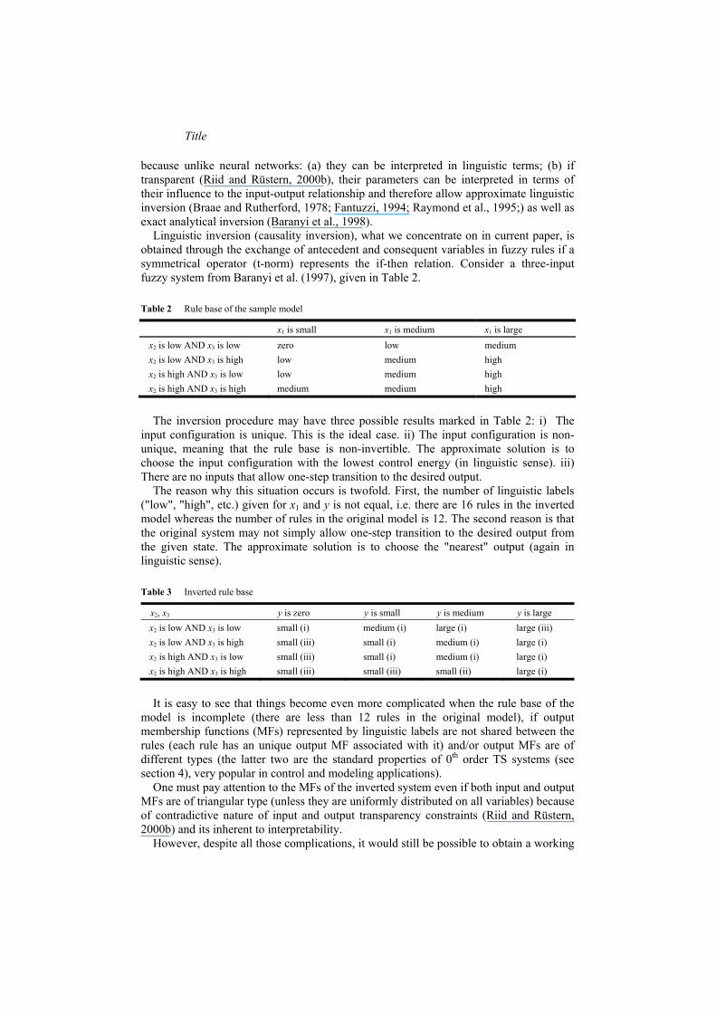
Title
because unlike neural networks (a) they can be interpreted in linguistic terms (b) if transparent (Riid and Ruumlstern 2000b) their parameters can be interpreted in terms of their influence to the input-output relationship and therefore allow approximate linguistic inversion (Braae and Rutherford 1978 Fantuzzi 1994 Raymond et al 1995) as well as exact analytical inversion (Baranyi et al 1998)
Linguistic inversion (causality inversion) what we concentrate on in current paper is obtained through the exchange of antecedent and consequent variables in fuzzy rules if a symmetrical operator (t-norm) represents the if-then relation Consider a three-input fuzzy system from Baranyi et al (1997) given in Table 2
Table 2 Rule base of the sample model
x1 is small x1 is medium x1 is large
x2 is low AND x3 is low zero low medium x2 is low AND x3 is high low medium high x2 is high AND x3 is low low medium high x2 is high AND x3 is high medium medium high
The inversion procedure may have three possible results marked in Table 2 i) The
input configuration is unique This is the ideal case ii) The input configuration is non-unique meaning that the rule base is non-invertible The approximate solution is to choose the input configuration with the lowest control energy (in linguistic sense) iii) There are no inputs that allow one-step transition to the desired output
The reason why this situation occurs is twofold First the number of linguistic labels (low high etc) given for x1 and y is not equal ie there are 16 rules in the inverted model whereas the number of rules in the original model is 12 The second reason is that the original system may not simply allow one-step transition to the desired output from the given state The approximate solution is to choose the nearest output (again in linguistic sense)
Table 3 Inverted rule base
x2 x3 y is zero y is small y is medium y is large
x2 is low AND x3 is low small (i) medium (i) large (i) large (iii) x2 is low AND x3 is high small (iii) small (i) medium (i) large (i) x2 is high AND x3 is low small (iii) small (i) medium (i) large (i) x2 is high AND x3 is high small (iii) small (iii) small (ii) large (i)
It is easy to see that things become even more complicated when the rule base of the
model is incomplete (there are less than 12 rules in the original model) if output membership functions (MFs) represented by linguistic labels are not shared between the rules (each rule has an unique output MF associated with it) andor output MFs are of different types (the latter two are the standard properties of 0th order TS systems (see section 4) very popular in control and modeling applications)
One must pay attention to the MFs of the inverted system even if both input and output MFs are of triangular type (unless they are uniformly distributed on all variables) because of contradictive nature of input and output transparency constraints (Riid and Ruumlstern 2000b) and its inherent to interpretability
However despite all those complications it would still be possible to obtain a working
Author
inversion for control purposes if we have a specification for desired closed control loop behavior Assume that our control goal is to achieve a closed loop mapping that is defined in the left box in Figure 3
From the rules of the model that have linguistically identical premises in terms of x2 and x3 (ie rows in Table 1) only one that corresponds to the desired label of y is selected and inverted (Figure 3)
Figure 3 Closed loop behavior-oriented linguistic inversion
Clearly there are advantages with the proposed approach ndash the inverted model has Sy (the number of linguistic labels of y) times less rules than the original partial linguistic inversion and if the closed-loop specification is realistic we do not encounter (ii) and (iii) type rules The main disadvantage is that if the specification for closed-loop behavior is changed the model must be re-inverted again However it will be shortly shown (in section 4) that it is possible to automate the inversion procedure Figure 4 Partition state and output variables
The proposed closed loop inversion is an improvement over partial inversion scheme
also numerically as the following example demonstrates We give numerical background to rule bases above the by using the partitions for variables x1 x2 x3 and y as depicted in Figure 4 and assuming product-product-sum inference For comparison of different inversion techniques we employ a scheme depicted in Figure 5 where yprime is the output of closed loop specification that can be found in the upper box Figure 3 yprimeprime is the output of the control object (Table 1) when controlled by the controller that is obtained through partial inversion (Table 2) and yprimeprimeprime is objectrsquos output when it is governed by closed loop inversion (lower box in Figure 3) It turns out that yprime and yprimeprimeprime are totally equivalent
-05 0 05 1 150
05 1
x1
small medium large
0 02 04 06 08 10
05 1
x2 x3
low high
-01 0 01 02 03 040
05 1
y
zero low medium high
IF x2 is low AND x3 is low THEN y is lowIF x2 is low AND x3 is high THEN y is medium IF x2 is high AND x3 is low THEN y is high IF x2 is high AND x3 is high THEN y is high
desired closed loop behavior
IF x2 is low AND x3 is low THEN x1 is medium IF x2 is low AND x3 is high THEN x1 is medium IF x2 is high AND x3 is low THEN x1 is large IF x2 is high AND x3 is high THEN x1 is large
corresponding profile of x1
Title
whereas there is a marked difference between yprime and yprimeprime (Figure 6) that proves our point Sure this is a somewhat engineered example because there is no model-plant mismatch and the input and output MFs (see Figure 4) are chosen such that no transparency constraints are violated by inversion But even in situations when these conditions are violated inversion error would be smaller with proposed inversion scheme than with partial inversion Figure 5 Comparison of inversion schemes
41 Obtaining the model The first step in controller design is the generation of the 0th order Takagi-Sugeno
model of the fermentation process having the following structure
IF x is A1r AND s1 is A2r AND s2 is A3rTHEN ∆x is b1r AND ∆p = b2r (4) where Air denote the linguistic labels (such as ldquosmallrdquo ldquohotrdquo etc) of the input variables and bjr are the scalar values of output variables - growth of biomass (∆x = x(k) - x(k - 1)) and growth of the product (∆p = p(k) - p(k - 1) k = 2 hellip K) associated with the rth rule (i = 1 3 j = 1 2 r = 1 R)
0th order TS systems possess computationally inexpensive inference algorithm that gives numerical relationship between the system (4) variables
sumsum==
=R
rr
R
rjrrj by
11
ττ
(5)
where τr is the activation degree of the r-th rule given by
prod=
=N
iiirr x
1
)(microτ
(6)
where microir denotes the MF (membership function) of the ith input variable (representing Air) associated with the rth rule
In current application our primary concern is the ability to discover valid causal relationships between system variables and therefore both transparency and reliability of the fuzzy model are important requirements The concept of transparency (validity of linguistic interpretation) has been discussed extensively in our previous works (eg Riid and Ruumlstern 2003) and it has been found out that transparency can be preserved by
control object
X2
X3
yprimeprime
partial inversion
closed loop
inversion
closed loop spec
yprime
control object yprimeprimeprime
Author
imposing certain restrictions to MF parameters Figure 6 Desired output profile (yprime) system output through closed loop inversion (yprimeprimeprime) system output through
partial inversion (yprimeprime) and the inversion error (yprime - yprimeprime)
In order to satisfy input transparency conditions (output constraint is satisfied by default with current model configuration) we require triangular input MFs (given by parameters i
si
si
si Sscba 1 = see Fig 3) to form a partition (7) ndash ie
11 +minus == si
si
si
si bcba
sum=
=isinforalliS
si
siii xXx
1
1)( micro
(7)
The problem of reliability is addressed through the modeling algorithm that we use First of all for the identification of the input partition no real algorithm is used Given Si (i = 1 hellip N) input MFs per ith input variable these are distributed logarithmically along
005
1
005
10
02
04
x3x
2
yacuteacute
005
1
005
1-005
0
005
x3x
2
yacute-yacuteacute
005
1
005
10
02
04
x3
x2
yacute yacuteacuteacute
Title
the x-axis
1))1()1)((( minmaxmini
miiii
si SsSsxxxb =minusminusminus+= (8)
where s
ib is the core of the observed MF (Figure 3) and m gt 0 is the exponent It is easy to see that with 0 lt m lt 1 higher values of xi are modeled with greater resolution with m = 1 we have uniform distribution and with m gt 1 smaller quantities of xi are modeled with greater resolution (as in Figure 8)
Figure 7 Input partition style employed in current study
0
05
1 simicro 1+s
imicro
sib
hellip hellip
1+= si
si bc1minus= s
isi ba
1minussimicro
x
micro
Figure 8 Logarithmic input partition (m = 2)
Given such input partition it is possible to consider up to Rmax = S1sdotS2sdothellipsdotSN rules (all
possible antecedent combinations) However each rule is checked for validity before adding it to the model by comparing max(τr(k)) (k = 1 hellip K) to some pre-specified threshold value and added only if the former exceeds that
Moreover consequent parameters of all M output variables of the rth rule are computed simultaneously with the creation of rules using the method of Nozaki et al (1997)
sumsum==
=K
kr
K
kjrjr kkykb
11
))(()())(( αα ττ
(9)
where α is the parameter that influences model accuracy in terms of RMSE (root-mean-squared-error) For example it is reported in Nozaki et al (1997) that α = 10 provides best results in ideal environment and that it should be smaller if data is bad for current application (section 6) best results were obtained with α = 2
Thus reliability of the model is addressed in two ways ndash rule validity routine helps to filter out the rules that are not really evidenced by available training data (and keeps the model compact as well) and as the consequent parameters for the given rule are computed as the weighted average of relevant (measured by rule activation degree τr in (7)) output samples it gives the model interpolating rather than extrapolating character
minix
0
1
sib max
ix
Author
42 Automatic Inversion of the Model Once the model is obtained the extracted rules are grouped into Sx subsets (Sx is the
number of MFs defined for biomass and consequently each subgroup contains the rules that have the same label of x) and inverted (Figure 9) Figure 9 An example of linguistic inversion of the fed-batch fermentation model Selection and inversion of
the rule belonging to the subgroup where x is ldquolargerdquo (L stands for large S for small VS for very small Z for zero) The highlighted rule is chosen for inversion because it provides the biggest growth rate for p
Figure 10 Decision making mechanism and its parameters
As shown in Riid and Ruumlstern (2006) the selection and inversion task can be performed automatically All numerical values of (b1r b2r) corresponding to the rules of the given subgroup are then fed into respective inputs of the decision making mechanism (Figure 10) that computes the corresponding pair (τ1 τ2) Of the subset of rules the one with maximum τ1 or τ2 (whichever happens to be larger) is declared the winner and inverted - rewritten in the format
IF x is A1r THEN s1 = p1r AND s2 = p2r (10) where p1r = core(A2r) p2r = core(A3r)
IF x is large THEN s1 is very_small amp s2 is zero
IF x is large amp amp s1 is VS amp s2 is S THEN ∆x is S amp ∆p is S amp s1 is VS amp s2 is Z THEN ∆x is S amp ∆p is L
amp s1 is Z amp s2 is Z THEN ∆x is Z amp ∆p is Z amp s1 is Z amp s2 is VS THEN ∆x is VS amp ∆p is Z
amp s1 is S amp s2 is VS THEN ∆x is L amp ∆p is S
∆xmax∆xmin
∆pmax∆pmin
micro11 micro12
micro21 micro22
micro11 ∆x
Π
Π micro12
micro22
micro21 ∆p
τ1
τ2
Title
Figure 11 Hierarchical control system for manipulation of substrate concentrations in the fermenter
The resulting controller or process manager consisting of Sx rules will then be
embedded into the control system where PI controllers take care of the substrate flow regulation (Figure 11)
So the sequence from the process to the functioning controller can be seen as in Figure 12 Figure 12 Controller design procedure
5 Evolutionary algorithms and IEC Evolutionary algorithm (EA) is a generic population-based metaheuristic optimization
algorithm that uses some mechanisms inspired by biological evolution (eg mutation recombination and selection) A population consists of candidate solutions to the optimization problem and the environment in which the solutions live is specified by a fitness function Evolution of the population takes place after the repeated application of the biology-inspired operators Evolutionary algorithms are useful as they do not make
P
Fermentor
Process manager
s1 x
f2
s2
f1
r1r2
P
original process
x s1 s2 p V f1 f2
process model
s1 s2
∆x∆p
x
control manager
x s1
s2
Author
any assumptions about the underlying fitness landscape and are therefore (at least theoretically) able to find approximate solutions to all types of problems
Usually the initial population consists of randomly generated candidate solutions The fitness function is applied to the candidate solutions and any subsequent offspring Figure 13 Typical flowchart for an evolutionary algorithm
By selection parents for the next generation are chosen with a bias towards higher
fitness The parents reproduce by recombination andor mutation Recombination acts on two selected parents and results in one or two children Mutation acts on one candidate and results in a new candidate These operators create the offspring (a set of new candidates) New candidates compete with old candidates for their place in the next generation (survival of the fittest)
This process can be repeated until a candidate with sufficient quality is found or a previously determined computational limit is reached (Figure 13)
Depending on how the solutions are represented which search operators are used and how the selection process is carried out evolutionary algorithms can be divided into different classes of which evolution strategies and genetic algorithms stand out as most common
Evolution strategies (ESs) were developed in the 1960s by Rechenberg and his colleagues (Rechenberg 1973) Evolution strategies typically use fixed-length real-valued vectors for solution representation and primarily mutation and selection as search operators
As far as real-valued search spaces are concerned mutation is usually performed by adding a normally distributed random value to each vector component The step size or mutation strength (ie the standard deviation of the normal distribution) is often governed by self-adaptation Individual step sizes for each coordinate or correlations between coordinates are either governed by self-adaptation or by covariance matrix adaptation
The selection in evolution strategies is based on the fitness rankings The simplest ES operates on a population of size two the current point (parent) and the result of its mutation If the mutant has a higher fitness than the parent it becomes the parent of the next generation Otherwise the mutant is disregarded This is a (1 + 1)-ES More generally λ mutants can be generated and compete with the parent called (1 + λ)-ES In a (1 λ)-ES the best mutant becomes the parent of the next generation while the current parent is always disregarded
Genetic algorithms (GAs) became popular through the work of John Holland in the
initialize the population
apply selection
create offsprings
evaluate fitness terminate
no
yes
Title
early 1970s (Holland 1975) A standard representation of the solution in GAs is an array of bits The main property that makes such representation convenient is that its parts are easily aligned due to their fixed size that facilitates simple crossover operations
During each successive generation a proportion of the existing population is selected to breed a new generation fitter solutions are typically more likely to be selected Certain selection methods rate the fitness of each solution and preferentially select the best solutions Popular selection methods include roulette wheel selection and tournament selection Some methods rate only a random sample of the population as fitness evaluation may be very time-consuming
For each new solution to be produced a pair of parent solutions is picked for breeding from the pool selected previously By producing a child solution using the methods of crossover and mutation a new solution is created which typically shares many of the characteristics of its parents New parents are selected for each child and the process continues until a new population of solutions of appropriate size is generated
Most functions are stochastic and designed so that a small proportion of less fit solutions are selected This helps keep the diversity of the population large preventing premature convergence on poor solutions
The past few years have effectively seen the merge of these two methods into an even more powerful one (Mayer et al 1999) The typical trends in this are the adoption of real-valued genes in GAs (to more closely match problem definitions) and the introduction of recombination and crossover operations using multiple parents in ESs
51 Interactive Evolutionary Computation IEC (Madar et al 2003) is a (micro + λ) Evolution Strategy where λ offspring are
generated by recombination and mutation from micro parents The resulting micro + λ individuals are evaluated by the user who eventually selects the best micro parents to the next generation The selection process is supported by the program interface that visualizes variables under optimization However IEC can only use a moderate number of individuals and searching generations because of resulting human fatigue
IEC Toolbox can be downloaded from the website of its authors however for current fed-batch fermentation application considerable adjustments are necessary
In IEC it is assumed that each potential solution can be represented by a m-dimensional vector of x isin Rm of object variables To allow for a better adaptation to the objective functionrsquos topology the object variables are accompanied by a set of the so-called strategy parameters An individual ai = (xi σi) thus consists of two components ndash the object variables xi and up to m different standard deviations to control the step sizes σi = [σi1 hellip σim]T
In the mutation step random numbers generated by normal distributions zij ~ N(0 σij) are added to the individuals
xij = xij + zij (11) This introduces the principle from the nature where small changes occur frequently
but large ones rarely Before the object variables are changed the strategy parameters are mutated using a multiplicative normally distributed process
))10()10(( jNN
ijij e ττσσ += (12) where the first component of the exponent is a global factor that allows an overall
Author
change of the mutability and second accounts for individual changes of the mean step sizes τrsquo and τ can be interpreted in the sense of global learning rates and are given by
mm 2121 ==prime ττ (13)
Recombination is carried out by the following operations
sum ==prime==prime
micromicroσσ
1acute)1(
k kiiMjFjj mjxorxx (14)
where F and M are two selected individuals from the micro parent population
6 Application and results
61 Results by linguistic inversion First the effectiveness of the automatic inversion mechanism and reliability of the
model was tested by applying Nozakis algorithm to measured (and preprocessed) data from 10 process runs with nominal feeds (one can see the similarity with the approach taken in Zhang and Lennox (2003)) using the input partition depicted in Figure 14 that belongs to one of the successful controllers from Riid and Ruumlstern (2000a) Application of (7) resulted in a 38-rule (only so few are relevant of 140 potential rules according to the rule filter that has the threshold value at 0001) model that has RMSEs of 1075 and 018 for ∆p and ∆x respectively In the next step the model was inverted automatically into a four-rule process manager Averaged J (Jav) over ten process runs (132middot105) is 59 higher than the one corresponding to the nominal feed profiles and 29 higher than the number reported in Riid and Ruumlstern (2000a) that shows that the proposed inversion mechanism is more effective than mostly manual inversion and modeling approach taken in this work
However it is not always the case that the input partition is readily available In such cases we make educated guesses about the process Figure 14 Partition of the fuzzy model of Riid and Ruumlstern (2000)
10 20 30 400
05
1
x
10 20 300
05
1
s1
0 05 10 150
05
1
s2
In present application the concentration of biomass is regarded as the scheduling variable - its partition divides the process into separate stages for which we need to choose appropriate concentrations of substrates - so it is sufficient to consider few (4 or 5) uniformly distributed fuzzy sets for x The substrate concentrations however need to
Title
be modeled with greater resolution to provide rich information content Smaller substrate concentrations are more important (it is unlikely to maintain higher concentrations in the second phase of the process) therefore those areas are modeled with greater detail (m = 2)
As it is impossible to predict optimal partition beforehand several combinations of Si were tried out Table 4 contains the results of modeling and control (the figures are the average values of 10 process runs) Table 4 Results
Case RMSE (∆x∆p) partition R Jav pav Tav 1 02421288 4-8-8 47 110sdot105 3255 117 2 02599663 5-8-8 51 122sdot105 3012 97 3 02741146 4-9-9 56 125sdot105 3227 102 4 02681030 5-9-9 62 131sdot105 3063 92 5 0225871 4-10-10 66 113sdot105 3411 119 6 0225859 5-10-10 73 123sdot105 3263 105
There are yet additional ways for improving both the performance and consistency of
control First the problem with the control system depicted in Figure 11 is the high variance of results ndash eg process time (case 3) varies from 80 to 124 time units and product concentration from 2700 to 3400 during different runs In order to provide less variance we use averaged feed profiles (Figure 15) of 5 best process runs of tested 10 computed by the control system (Figure 11) which lead to much more consistent (as can be seen from Figure 16) and further improved (Jav = 128sdot105 T = 94 plusmn 4 pav = 3023 (2855-3130) results
Secondly from Figure 15 it is obvious that feed rate in the first quarter of the process is rather small which is ultimately the reason why it takes quite long time fill up the fermenter The process can be sped up by manipulating the value of p21 - the setpoint of s2 corresponding to the first quarter of the process ndash which currently is equal to 00235 When this is done in the range of 002 - 15 it appears that what we have got here is a very simple yet effective knob to influence process productivity and duration (the effect of this can be observed in Figure 24) It might be asked why importance of the value of p21 was not discovered in the modeling and inversion procedure in first place but the reason is really simple ndash the methodology improves control by exploiting available information but nominal feed profiles do not produce so high concentration of the substrate 2 in the first quarter of the process thus there was nothing to discover
Figure 15 Averaged feed profiles
0 10 20 30 40 50 60 70 80 900
10
20
30
40
50
T
f1
f2
Author
Figure 16 Control system performance over 10 process runs supervisory control system (left) averaged feed profiles (right)
62 Results by IEC In order to apply the IEC algorithm to the fed-batch fermentation it is necessary to
design a suitable representation of variable trajectories under optimization In current approach the profiles of these variables are divided into a number of segments Segment start times along with the corresponding values valid for considered variables in the segment is all we need to reconstruct the feed profiles (using simplistic stair-shaped trajectories better suited for this process instead of piecewise-linear ones implemented in Madar et al (2003)) During optimization the segments can shrink expand and obtain new values and that way the optimized variable profiles can change a great deal
621 Optimizing feed profiles with IEC In first case we optimize feed profiles directly thus do not need feedback from the
process other than in the end of each batch when we compute the productivity J to evaluate the current experiment
Feed profiles are encoded into chromosomes so that first half of the chromosome contains the segmentation scheduling information (separately for each of feed rates and excluding the zero one that is assumed by default in the encoding-decoding process to make the chromosome shorter) followed by values of f1 and f2 corresponding to defined segments For initialization a crude approximation of nominal feed profiles is provided (Figure 17)
Figure 17 Chromosome encoding and corresponding feed rates (prototype for the initial population)
0 50 1000
5
10
15x 4
0 50 1000
5
10
15x
4
T
J
0 50 10010
20
30
0 50 1000
1
2
3
30 50 70 50 65 80 10 17 28 35 35 175 175 0
segmentation schedule for f1
segmentation schedule for f2
segment values (f1)
segment values (f2)
f1 f2
T T
Title
To make up the stochastic nature of both the process and the optimization algorithm we conduct 5 separate optimization cycles The number of individuals in the population is 8 and the number of generations in each series is 20
For the selection procedure we have adopted the following strategy up to four best solutions of the generation are chosen as the parents for the next generation Generally the best one of these is paired with all others and second and third best ones are coupled as well In result the population in each generation contains 4 best solutions of the previous generation and 4 offsprings Note that due to noise the productivity measure alone may be slightly misleading at times because it can vary quite a bit for same feed profiles This is where visualization of all process variables is particularly helpful
Table 5 shows the final results (two best solutions per series) that outperform nominal productivity by 39-66 The learning curve is very smooth (Figure 18) and barely any of the offsprings shows lesser productivity than the nominal feed profiles Therefore the financial cost of the approach is kept minimal
It is possible to use a finer resolution ie a larger number of segments However this would make the search less convergent because of expanded search space and may not pay off in the end
Having a look at the optimized feed profiles (Figure 19) we can conclude that the process is a rather robust one because apparently quite different feed profiles yield similar results Table 5 Productivity of optimized feed profiles
Series no Best solution (J) Second best solution 1 13652sdot105 13372sdot105 2 11530sdot105 11457sdot105 3 13332sdot105 13242sdot105 4 12087sdot105 11580sdot105 5 12530sdot105 11709sdot105
Figure 18 Best solution of the population (105) of five optimization cycles
0 1 2
0 1 2
0 1 2 0 1 2
8 10 12 14 16 18 202 4 60 1 2
No of generations
J
Author
Figure 19 A selection of optimized feed profiles
622 Optimizing substrate concentrations with IEC Taking a step further and optimizing the substrate concentration profiles of s1 and s2 in
the fermenter by EC we no longer need x for scheduling (as in the scheme depicted in Figure 11) On the other hand we still need to measure substrate concentrations online
As with feed profiles optimization a crude approximation of setpoint trajectories from nominal substrate profiles was created that serves as the prototype for the initial population (Figure 20) Table 6 contains the results of optimization (two best solution per series are given) Figure 20 Chromosome encoding for substrate profile optimization and the prototype for initial population
Table 6 Optimization results (second series)
Series no Best solution (J) Second best solution 1 16465sdot105 16213sdot105 2 17016sdot105 16259sdot105 3 17496sdot105 14333sdot105 4 16934sdot105 15662sdot105 5 16924sdot105 16651sdot105
We can observe very strong performance improvement as nominal feed profiles are
now outperformed by 75-113 (this is also better than currently known best result for that process obtained in Liang and Chen (2003))
Compared to the previous optimization scenario the learning process is much more hectic and many potential solutions are subpar This is visualized in Figure 21 that brings
0 20 40 60 800
20
40
T
f1f2
0 20 40 60 800
20
40
T
f1 f2
0 20 40 60 800
20
40
T
f1f2
0 20 40 60 800
20
40
T
f1 f2
20 40 60 80 1000
10 20 30
20 40 60 80 1000
05
115
s1 s2
25 55 70 15 60 80 30 02 03 04 1 005 003 0 0
segmentation schedule for s1
segmentation schedule for s2
segment values (s1)
segment values (s2)
T
Title
out the productivity value of the best offspring in the generation Apparently optimization of s1 and s2 hits the sensitive spot of the process This however is somewhat compensated by faster convergence
Figure 21 Productivity (105) of the fittest offsping in the population (five optimization cycles)
Let us have a closer look what really happens in the fermenter with one of the best yet the simplest substrate profiles (Figure 22) It can be seen that the prescribed value of s1 is achieved rather quickly compared to s2 At around T = 23 the setpoint for s2 becomes equal to zero This moment also marks the beginning of rapid biomass growth which quickly reduces s1 in the fermenter despite that f1 is full on As soon as s2 actually reaches zero biomass growth slows down and rapid product growth starts The latter slows down even before than f1 is considerably reduced and continues to grow with moderate pace till the fermenter volume limit is reached that ends the process Similar process flow can be observed with suboptimal controllers the difference is that with the optimal feedsubstrate profiles everything happens very quickly as the feed rates are quite high throughout the batch
A familiar problem characteristic to the supervisory control scheme is that the variance of results is quite high As before we may use averaged feed profiles of 5 best process runs of tested 10 computed by PI controllers in the control system (Figure 11) that while reducing the average productivity from 169105 to 163105 lead to much more consistent results (Figure 23)
7 Conclusions The properties of the fed-batch fermentation benchmark that resemble real-life
characteristics - presence of noise random variations of state variables parameter drift and ultimately the MIMO nature of the process - make it very difficult to be controlled by traditional means The fact that the orthodox optimal control approach taken in Becerra and Roberts (1998) yields only moderately successful results is a case in point Approximate techniques endorsed by computational intelligence paradigm on the other
1 2 3 4 5 6 7 8 9 100
1
2J
0
1 2
1
15
2
No of generations
1 2 3 4 5 6 7 8 9 100
1
21 2 3 4 5 6 7 8 9 10
0
1
2
1 2 3 4 5 6 7 8 9 10
1 2 3 4 5 6 7 8 9 10
Author
hand are more flexible and as our experiments show also more efficient in information analysis or knowledge acquisition particularly when we are able to properly choose the variable profiles which are going to be optimized (ie optimization of substrate concentrations instead of perhaps more obvious choice of feed rate optimization) that in the end leads to much improved control performance (Figure 24)
Figure 22 Fermentation process with computed setpoint profiles Above product (bold line) and biomass
(normal line) concentrations In the middle Set profiles (slashed lines) vs actual substrate concentrations Below Feed rates 1 (bold line) and 2 (normal line)
Figure 23 Results by IEC before and after averaging the feed profiles
The main challenge with many industrial processes is that even if what we need to
10 20 30 40 50 600
1000
2000 3000
10 20 30 40 50 600
10
20
30
40
0
20
40
20
40
60
0
xp
s1s2
f1f2
10 20 30 40 60T
r2 r1
f1 f2
10 20 30 40 500
05
1
15
2x10
5
10 20 30 40 500
20
40
T T
J
10 20 30 40 50 60 700
05 1
15 2
x10 5
Title
know may be quite simple it is very hard to discover or to learn it in the first place The fed-batch fermentation serves as an adequate example of this situation because even two-segment feed profiles would be sufficient for good performance as Figure 25 amply demonstrates But the discovery that the solution turns out to be simple is just an afterthought in present case
Figure 24 Productivity vs process duration Comparison - results by linguistic inversion (with different
values of p21 which are indicated in the figure) ndash IEC1 - IEC2 - LC1 - LC2 + - DISOPE loz ndash MOC1 diams - MOC2 x - nominal feed profiles
Figure 25 A selection of optimized substrate concentrations
The computational intelligence techniques presented in current paper have both their
advantages and disadvantages For example the linguistic inversion technique that has its advantage for making the design process very transparent is designed so that it aims at maximization of product concentration rather than J and it is therefore more difficult to influence the general dynamics of the process (ie its duration) The latter problem may be a matter of further research
Evolutionary computation on the other hand is more efficient in maximizing J as it searches solution space exhaustively However its computational (and financial) cost may become inhibitive for certain applications
50 100 15005
1
15
2x 10 5
T
J
x
002
05075
15 10
125
10 30T
40T
0 20 400
20 40
T
r1r2
0 20 40 600
20
40
T
r1r2
0 20 400
20 40
r1 r2
0 20 600
20
40
r1r2
Author
References Babuška R (1998) Fuzzy Modeling for Control Kluwer Academic Publishers Boston Baranyi P Bavelaar IM Babuška R Koacuteczy LT Titli A and Verbruggen HB (1998) lsquoA
method to invert a linguistic fuzzy modelrsquo Int J Systems Science Vol 29 No 7 pp711-721 Becerra V M and Roberts P D (1998) lsquoApplication of a novel optimal control algorithm to a
benchmark fed-batch fermentation processrsquoTrans Inst MC Vol 20 No 1 pp11-18 Braae M and Rutherford DA (1979) lsquoTheoretical and Linguistic Aspects of the Fuzzy Logic
Controllerrsquo Automatica Vol 15 No 5 pp553-577 Broyden CG (1965) lsquoA class of methods for solving nonlinear simultaneous equationsrsquo Math
Comp Vol 19 pp577ndash593 Fantuzzi C (1994) lsquoLinguistic rule synthesis of A fuzzy logic controllerrsquo ProcIECON94 pp
1354-1358 Hewitt CJ and Nienow AW (2007) lsquoThe scale-up of microbial batch and fed-batch
fermentation processesrsquo Adv Appl Microbiol Vol 62 pp105-135 Holland JH (1975) Adaptation in natural and artificial systems The University of Michigan
Press Ann Arbor Holmblad LP and Ostergaard J-J lsquoControl of a cement kiln by fuzzy logicrsquo in Gupta MM and
Sanchez E (1982) Fuzzy Information and Decision Processes North-Holland Publishing Company Amsterdam pp389ndash399
Hough P D Kolda T G and Torczon V J (2001) lsquoAsynchronous parallel pattern search for nonlinear optimizationrsquo SIAM J Sci Comput Vol 23 pp134ndash156
Kawohl M Heine T and King R (2007) lsquoModel based estimation and optimal control of fed-batch fermentation processes for the production of antibioticsrsquo Chemical engineering and processing Vol 46 No 11 pp1223-1241
Jang J-S R Sun C-T and Mizutani E (1996) Neuro-Fuzzy and Soft Computing A Computational Approach to Learning and Machine Intelligence Prentice Hall Upper Saddle River
Jensen CA Reed RD Marks RJ El-Sharkawi MA Jung J-B Miyamoto RT Anderson GM and Eggen CJ (1999) lsquoInversion of feedforward neural networks Algorithms and applicationsrsquo Proceedings of the IEEE Vol 87 No 9 pp1536-1549
Leigh R (1998) lsquoFed-batch fermentation process modelling and control competitionrsquo Trans Inst MC Vol 20 No 1 p3
Liang J and Chen Y (2003) lsquoOptimization of a fed-batch fermentation process control competition problem using the NEOS serverrsquo Proc Inst Mech Engrs Part I J Systems Control Eng Vol 217 Part 5 pp427-432
Liang J Chen Y Meng MQ-H and Fullmer R (2003) lsquoSolving Tough Optimal Control Problem by Network Enabled Optimization Server (NEOS)rsquo Proc IEEE Intelligent Automation Conf
Lotfi A Andersen H C and Tsoi A C (1996) lsquoInterpretation Preservation of Adaptive Fuzzy Inference Systemsrsquo Int J Approximate Reasoning Vol 15 No 4 pp379-394
Ma Y (2007) lsquoResearch on On-Line Modeling of Fed-Batch Fermentation Process Based on v-SVRrsquo in Huang D-S Heutte L and Loog M (eds) Advanced Intelligent Computing Theories and ApplicationsWith Aspects of Artificial Intelligence Springer pp900-908
Madaacuter J Abonyi J and Szeifert F (2003) lsquoInteractive Evolutionary Computation for model based Optimization of Batch Fermentationrsquo IASTED International Conference on Artificial Intelligence and Applications Benalmaacutedena Spain pp100-105
Mayer DG Belward JA Widell H and Burrage K (1999) lsquoSurvival of the fittestmdash algorithms versus evolution strategies in the optimization of systems modelsrsquo Agricultural Systems Vol 60 No 2 pp113-122
Title
McKay B Sanderson CS Willis MJ Bartford JP and Barton GW (1998) lsquoEvolving a hybrid model of a fed-batch fermentation processrsquo Trans Inst MC Vol 20 No 1 pp4-10
Nomikos P and MacGregor JF (1994) lsquoMonitoring batch processes using multiway principal component analysisrsquo AIChe Journal Vol 40 pp1361-75
Nozaki K Ishibuchi H and Tanaka H (1997) lsquoA simple but powerful heuristic method for generating fuzzy rules from numerical datarsquo Fuzzy Sets and Systems Vol 86 No 3 pp251-270
de Oliveira JV (1999) lsquoSemantic constraints for membership function optimizationrsquo IEEE Trans Systems Man and Cybernetics Vol 29 No 1 pp128 -138
Pedrycz W (editor) (1997) Fuzzy Evolutionary Computation Kluwer Aademic Publishers New York
Raymond C Boverie S and Titli A (1995) lsquoFuzzy multivariable control design from the fuzzy system modelrsquo Proc IFSA World Congr pp509-511
Rechenberg I (1973) Evolutionsstrategie - Optimierung technischer Systeme nach Prinzipien der biologischen Evolution Frommann-Holzboog Stuttgart
Riid A and E Ruumlstern E (2000a) lsquoSupervisory fed-batch fermentation control on the basis of linguistically interpretable fuzzy modelsrsquo Proc Estonian Acad Sci Eng Vol 6 No 2 pp96-112
Riid A and E Ruumlstern E (2000b) lsquoTransparent fuzzy systems and modeling with transparency protectionrsquo Proc IFAC Symp on Artificial Intelligence in Real Time Control pp229-234
Riid A and Ruumlstern E (2003) lsquoTransparent Fuzzy Systems in Modeling and Controlrsquo in Casillas J Cordon O Herrera F and Magdalena L (editors) Interpretability Issues in Fuzzy Modeling Springer pp452-476
Riid A and E Ruumlstern E (2006) lsquoAutomatic Linguistic Inversion of a Fuzzy Model for Fed-Batch Fermentation Controlrsquo Proc10th Int Conf Intelligent Engineering Systems pp129-134
Riid A and E Ruumlstern E (2007) lsquoInterpretability of Fuzzy Systems and Its Application to Process Controlrsquo Proc IEEE Int Conf Fuzzy Systems pp 1-6
Riid A and E Ruumlstern E (2008) lsquoFed-Batch Fermentation Controller Design with Evolutionary Computationrsquo Proc 5th ACMIEEE Int Conf Soft Computing as Transdisciplinary Science and Technology pp371-377
Soufian M and Soufian M (1997) lsquoParallel Genetic Algorithms for Optimised Fuzzy Modelling with application to a Fermentation Processrsquo Proc 2nd Int Conf on Genetic Algorithms In Engineering Systems Innovations and Applications pp123-128
Soufian M Soufian M and Dempsey MJ (1998) lsquoThe Effect of a Dynamical Layer in Neural Network Prediction of Biomass in a Fermentation ProcessrsquoLecture notes in computer science Vol 1415 pp749-757
Takagi T and Sugeno M (1985) lsquoFuzzy identification of systems and its applications to modeling and controlrsquo IEEE Trans Syst Man Cybern Vol SMC-15 No 1 pp116-132
Zhang H and Lennox B (2003) lsquoMulti-way optimal contol of a benchmark fed-batch fermentation processrsquo Trans Inst MC Vol 25 No 5 pp403-417
Zhang H Lennox B Goulding PR and Leung AYT (2000) lsquoA float-encoded genetic algorithm technique for integrated optimization of piezoelectric actuator and sensor placement and feedback gainsrsquo Smart Mater Struct Vol 9 pp552ndash557
Zhang H (2008) lsquoOptimal control of a fed-batch yeast fermentation process based on Least Square Support Vector Machinersquo Int J Engineering Systems Modelling and Simulation Vol 1 No 1 pp63-68

Author
inversion for control purposes if we have a specification for desired closed control loop behavior Assume that our control goal is to achieve a closed loop mapping that is defined in the left box in Figure 3
From the rules of the model that have linguistically identical premises in terms of x2 and x3 (ie rows in Table 1) only one that corresponds to the desired label of y is selected and inverted (Figure 3)
Figure 3 Closed loop behavior-oriented linguistic inversion
Clearly there are advantages with the proposed approach ndash the inverted model has Sy (the number of linguistic labels of y) times less rules than the original partial linguistic inversion and if the closed-loop specification is realistic we do not encounter (ii) and (iii) type rules The main disadvantage is that if the specification for closed-loop behavior is changed the model must be re-inverted again However it will be shortly shown (in section 4) that it is possible to automate the inversion procedure Figure 4 Partition state and output variables
The proposed closed loop inversion is an improvement over partial inversion scheme
also numerically as the following example demonstrates We give numerical background to rule bases above the by using the partitions for variables x1 x2 x3 and y as depicted in Figure 4 and assuming product-product-sum inference For comparison of different inversion techniques we employ a scheme depicted in Figure 5 where yprime is the output of closed loop specification that can be found in the upper box Figure 3 yprimeprime is the output of the control object (Table 1) when controlled by the controller that is obtained through partial inversion (Table 2) and yprimeprimeprime is objectrsquos output when it is governed by closed loop inversion (lower box in Figure 3) It turns out that yprime and yprimeprimeprime are totally equivalent
-05 0 05 1 150
05 1
x1
small medium large
0 02 04 06 08 10
05 1
x2 x3
low high
-01 0 01 02 03 040
05 1
y
zero low medium high
IF x2 is low AND x3 is low THEN y is lowIF x2 is low AND x3 is high THEN y is medium IF x2 is high AND x3 is low THEN y is high IF x2 is high AND x3 is high THEN y is high
desired closed loop behavior
IF x2 is low AND x3 is low THEN x1 is medium IF x2 is low AND x3 is high THEN x1 is medium IF x2 is high AND x3 is low THEN x1 is large IF x2 is high AND x3 is high THEN x1 is large
corresponding profile of x1
Title
whereas there is a marked difference between yprime and yprimeprime (Figure 6) that proves our point Sure this is a somewhat engineered example because there is no model-plant mismatch and the input and output MFs (see Figure 4) are chosen such that no transparency constraints are violated by inversion But even in situations when these conditions are violated inversion error would be smaller with proposed inversion scheme than with partial inversion Figure 5 Comparison of inversion schemes
41 Obtaining the model The first step in controller design is the generation of the 0th order Takagi-Sugeno
model of the fermentation process having the following structure
IF x is A1r AND s1 is A2r AND s2 is A3rTHEN ∆x is b1r AND ∆p = b2r (4) where Air denote the linguistic labels (such as ldquosmallrdquo ldquohotrdquo etc) of the input variables and bjr are the scalar values of output variables - growth of biomass (∆x = x(k) - x(k - 1)) and growth of the product (∆p = p(k) - p(k - 1) k = 2 hellip K) associated with the rth rule (i = 1 3 j = 1 2 r = 1 R)
0th order TS systems possess computationally inexpensive inference algorithm that gives numerical relationship between the system (4) variables
sumsum==
=R
rr
R
rjrrj by
11
ττ
(5)
where τr is the activation degree of the r-th rule given by
prod=
=N
iiirr x
1
)(microτ
(6)
where microir denotes the MF (membership function) of the ith input variable (representing Air) associated with the rth rule
In current application our primary concern is the ability to discover valid causal relationships between system variables and therefore both transparency and reliability of the fuzzy model are important requirements The concept of transparency (validity of linguistic interpretation) has been discussed extensively in our previous works (eg Riid and Ruumlstern 2003) and it has been found out that transparency can be preserved by
control object
X2
X3
yprimeprime
partial inversion
closed loop
inversion
closed loop spec
yprime
control object yprimeprimeprime
Author
imposing certain restrictions to MF parameters Figure 6 Desired output profile (yprime) system output through closed loop inversion (yprimeprimeprime) system output through
partial inversion (yprimeprime) and the inversion error (yprime - yprimeprime)
In order to satisfy input transparency conditions (output constraint is satisfied by default with current model configuration) we require triangular input MFs (given by parameters i
si
si
si Sscba 1 = see Fig 3) to form a partition (7) ndash ie
11 +minus == si
si
si
si bcba
sum=
=isinforalliS
si
siii xXx
1
1)( micro
(7)
The problem of reliability is addressed through the modeling algorithm that we use First of all for the identification of the input partition no real algorithm is used Given Si (i = 1 hellip N) input MFs per ith input variable these are distributed logarithmically along
005
1
005
10
02
04
x3x
2
yacuteacute
005
1
005
1-005
0
005
x3x
2
yacute-yacuteacute
005
1
005
10
02
04
x3
x2
yacute yacuteacuteacute
Title
the x-axis
1))1()1)((( minmaxmini
miiii
si SsSsxxxb =minusminusminus+= (8)
where s
ib is the core of the observed MF (Figure 3) and m gt 0 is the exponent It is easy to see that with 0 lt m lt 1 higher values of xi are modeled with greater resolution with m = 1 we have uniform distribution and with m gt 1 smaller quantities of xi are modeled with greater resolution (as in Figure 8)
Figure 7 Input partition style employed in current study
0
05
1 simicro 1+s
imicro
sib
hellip hellip
1+= si
si bc1minus= s
isi ba
1minussimicro
x
micro
Figure 8 Logarithmic input partition (m = 2)
Given such input partition it is possible to consider up to Rmax = S1sdotS2sdothellipsdotSN rules (all
possible antecedent combinations) However each rule is checked for validity before adding it to the model by comparing max(τr(k)) (k = 1 hellip K) to some pre-specified threshold value and added only if the former exceeds that
Moreover consequent parameters of all M output variables of the rth rule are computed simultaneously with the creation of rules using the method of Nozaki et al (1997)
sumsum==
=K
kr
K
kjrjr kkykb
11
))(()())(( αα ττ
(9)
where α is the parameter that influences model accuracy in terms of RMSE (root-mean-squared-error) For example it is reported in Nozaki et al (1997) that α = 10 provides best results in ideal environment and that it should be smaller if data is bad for current application (section 6) best results were obtained with α = 2
Thus reliability of the model is addressed in two ways ndash rule validity routine helps to filter out the rules that are not really evidenced by available training data (and keeps the model compact as well) and as the consequent parameters for the given rule are computed as the weighted average of relevant (measured by rule activation degree τr in (7)) output samples it gives the model interpolating rather than extrapolating character
minix
0
1
sib max
ix
Author
42 Automatic Inversion of the Model Once the model is obtained the extracted rules are grouped into Sx subsets (Sx is the
number of MFs defined for biomass and consequently each subgroup contains the rules that have the same label of x) and inverted (Figure 9) Figure 9 An example of linguistic inversion of the fed-batch fermentation model Selection and inversion of
the rule belonging to the subgroup where x is ldquolargerdquo (L stands for large S for small VS for very small Z for zero) The highlighted rule is chosen for inversion because it provides the biggest growth rate for p
Figure 10 Decision making mechanism and its parameters
As shown in Riid and Ruumlstern (2006) the selection and inversion task can be performed automatically All numerical values of (b1r b2r) corresponding to the rules of the given subgroup are then fed into respective inputs of the decision making mechanism (Figure 10) that computes the corresponding pair (τ1 τ2) Of the subset of rules the one with maximum τ1 or τ2 (whichever happens to be larger) is declared the winner and inverted - rewritten in the format
IF x is A1r THEN s1 = p1r AND s2 = p2r (10) where p1r = core(A2r) p2r = core(A3r)
IF x is large THEN s1 is very_small amp s2 is zero
IF x is large amp amp s1 is VS amp s2 is S THEN ∆x is S amp ∆p is S amp s1 is VS amp s2 is Z THEN ∆x is S amp ∆p is L
amp s1 is Z amp s2 is Z THEN ∆x is Z amp ∆p is Z amp s1 is Z amp s2 is VS THEN ∆x is VS amp ∆p is Z
amp s1 is S amp s2 is VS THEN ∆x is L amp ∆p is S
∆xmax∆xmin
∆pmax∆pmin
micro11 micro12
micro21 micro22
micro11 ∆x
Π
Π micro12
micro22
micro21 ∆p
τ1
τ2
Title
Figure 11 Hierarchical control system for manipulation of substrate concentrations in the fermenter
The resulting controller or process manager consisting of Sx rules will then be
embedded into the control system where PI controllers take care of the substrate flow regulation (Figure 11)
So the sequence from the process to the functioning controller can be seen as in Figure 12 Figure 12 Controller design procedure
5 Evolutionary algorithms and IEC Evolutionary algorithm (EA) is a generic population-based metaheuristic optimization
algorithm that uses some mechanisms inspired by biological evolution (eg mutation recombination and selection) A population consists of candidate solutions to the optimization problem and the environment in which the solutions live is specified by a fitness function Evolution of the population takes place after the repeated application of the biology-inspired operators Evolutionary algorithms are useful as they do not make
P
Fermentor
Process manager
s1 x
f2
s2
f1
r1r2
P
original process
x s1 s2 p V f1 f2
process model
s1 s2
∆x∆p
x
control manager
x s1
s2
Author
any assumptions about the underlying fitness landscape and are therefore (at least theoretically) able to find approximate solutions to all types of problems
Usually the initial population consists of randomly generated candidate solutions The fitness function is applied to the candidate solutions and any subsequent offspring Figure 13 Typical flowchart for an evolutionary algorithm
By selection parents for the next generation are chosen with a bias towards higher
fitness The parents reproduce by recombination andor mutation Recombination acts on two selected parents and results in one or two children Mutation acts on one candidate and results in a new candidate These operators create the offspring (a set of new candidates) New candidates compete with old candidates for their place in the next generation (survival of the fittest)
This process can be repeated until a candidate with sufficient quality is found or a previously determined computational limit is reached (Figure 13)
Depending on how the solutions are represented which search operators are used and how the selection process is carried out evolutionary algorithms can be divided into different classes of which evolution strategies and genetic algorithms stand out as most common
Evolution strategies (ESs) were developed in the 1960s by Rechenberg and his colleagues (Rechenberg 1973) Evolution strategies typically use fixed-length real-valued vectors for solution representation and primarily mutation and selection as search operators
As far as real-valued search spaces are concerned mutation is usually performed by adding a normally distributed random value to each vector component The step size or mutation strength (ie the standard deviation of the normal distribution) is often governed by self-adaptation Individual step sizes for each coordinate or correlations between coordinates are either governed by self-adaptation or by covariance matrix adaptation
The selection in evolution strategies is based on the fitness rankings The simplest ES operates on a population of size two the current point (parent) and the result of its mutation If the mutant has a higher fitness than the parent it becomes the parent of the next generation Otherwise the mutant is disregarded This is a (1 + 1)-ES More generally λ mutants can be generated and compete with the parent called (1 + λ)-ES In a (1 λ)-ES the best mutant becomes the parent of the next generation while the current parent is always disregarded
Genetic algorithms (GAs) became popular through the work of John Holland in the
initialize the population
apply selection
create offsprings
evaluate fitness terminate
no
yes
Title
early 1970s (Holland 1975) A standard representation of the solution in GAs is an array of bits The main property that makes such representation convenient is that its parts are easily aligned due to their fixed size that facilitates simple crossover operations
During each successive generation a proportion of the existing population is selected to breed a new generation fitter solutions are typically more likely to be selected Certain selection methods rate the fitness of each solution and preferentially select the best solutions Popular selection methods include roulette wheel selection and tournament selection Some methods rate only a random sample of the population as fitness evaluation may be very time-consuming
For each new solution to be produced a pair of parent solutions is picked for breeding from the pool selected previously By producing a child solution using the methods of crossover and mutation a new solution is created which typically shares many of the characteristics of its parents New parents are selected for each child and the process continues until a new population of solutions of appropriate size is generated
Most functions are stochastic and designed so that a small proportion of less fit solutions are selected This helps keep the diversity of the population large preventing premature convergence on poor solutions
The past few years have effectively seen the merge of these two methods into an even more powerful one (Mayer et al 1999) The typical trends in this are the adoption of real-valued genes in GAs (to more closely match problem definitions) and the introduction of recombination and crossover operations using multiple parents in ESs
51 Interactive Evolutionary Computation IEC (Madar et al 2003) is a (micro + λ) Evolution Strategy where λ offspring are
generated by recombination and mutation from micro parents The resulting micro + λ individuals are evaluated by the user who eventually selects the best micro parents to the next generation The selection process is supported by the program interface that visualizes variables under optimization However IEC can only use a moderate number of individuals and searching generations because of resulting human fatigue
IEC Toolbox can be downloaded from the website of its authors however for current fed-batch fermentation application considerable adjustments are necessary
In IEC it is assumed that each potential solution can be represented by a m-dimensional vector of x isin Rm of object variables To allow for a better adaptation to the objective functionrsquos topology the object variables are accompanied by a set of the so-called strategy parameters An individual ai = (xi σi) thus consists of two components ndash the object variables xi and up to m different standard deviations to control the step sizes σi = [σi1 hellip σim]T
In the mutation step random numbers generated by normal distributions zij ~ N(0 σij) are added to the individuals
xij = xij + zij (11) This introduces the principle from the nature where small changes occur frequently
but large ones rarely Before the object variables are changed the strategy parameters are mutated using a multiplicative normally distributed process
))10()10(( jNN
ijij e ττσσ += (12) where the first component of the exponent is a global factor that allows an overall
Author
change of the mutability and second accounts for individual changes of the mean step sizes τrsquo and τ can be interpreted in the sense of global learning rates and are given by
mm 2121 ==prime ττ (13)
Recombination is carried out by the following operations
sum ==prime==prime
micromicroσσ
1acute)1(
k kiiMjFjj mjxorxx (14)
where F and M are two selected individuals from the micro parent population
6 Application and results
61 Results by linguistic inversion First the effectiveness of the automatic inversion mechanism and reliability of the
model was tested by applying Nozakis algorithm to measured (and preprocessed) data from 10 process runs with nominal feeds (one can see the similarity with the approach taken in Zhang and Lennox (2003)) using the input partition depicted in Figure 14 that belongs to one of the successful controllers from Riid and Ruumlstern (2000a) Application of (7) resulted in a 38-rule (only so few are relevant of 140 potential rules according to the rule filter that has the threshold value at 0001) model that has RMSEs of 1075 and 018 for ∆p and ∆x respectively In the next step the model was inverted automatically into a four-rule process manager Averaged J (Jav) over ten process runs (132middot105) is 59 higher than the one corresponding to the nominal feed profiles and 29 higher than the number reported in Riid and Ruumlstern (2000a) that shows that the proposed inversion mechanism is more effective than mostly manual inversion and modeling approach taken in this work
However it is not always the case that the input partition is readily available In such cases we make educated guesses about the process Figure 14 Partition of the fuzzy model of Riid and Ruumlstern (2000)
10 20 30 400
05
1
x
10 20 300
05
1
s1
0 05 10 150
05
1
s2
In present application the concentration of biomass is regarded as the scheduling variable - its partition divides the process into separate stages for which we need to choose appropriate concentrations of substrates - so it is sufficient to consider few (4 or 5) uniformly distributed fuzzy sets for x The substrate concentrations however need to
Title
be modeled with greater resolution to provide rich information content Smaller substrate concentrations are more important (it is unlikely to maintain higher concentrations in the second phase of the process) therefore those areas are modeled with greater detail (m = 2)
As it is impossible to predict optimal partition beforehand several combinations of Si were tried out Table 4 contains the results of modeling and control (the figures are the average values of 10 process runs) Table 4 Results
Case RMSE (∆x∆p) partition R Jav pav Tav 1 02421288 4-8-8 47 110sdot105 3255 117 2 02599663 5-8-8 51 122sdot105 3012 97 3 02741146 4-9-9 56 125sdot105 3227 102 4 02681030 5-9-9 62 131sdot105 3063 92 5 0225871 4-10-10 66 113sdot105 3411 119 6 0225859 5-10-10 73 123sdot105 3263 105
There are yet additional ways for improving both the performance and consistency of
control First the problem with the control system depicted in Figure 11 is the high variance of results ndash eg process time (case 3) varies from 80 to 124 time units and product concentration from 2700 to 3400 during different runs In order to provide less variance we use averaged feed profiles (Figure 15) of 5 best process runs of tested 10 computed by the control system (Figure 11) which lead to much more consistent (as can be seen from Figure 16) and further improved (Jav = 128sdot105 T = 94 plusmn 4 pav = 3023 (2855-3130) results
Secondly from Figure 15 it is obvious that feed rate in the first quarter of the process is rather small which is ultimately the reason why it takes quite long time fill up the fermenter The process can be sped up by manipulating the value of p21 - the setpoint of s2 corresponding to the first quarter of the process ndash which currently is equal to 00235 When this is done in the range of 002 - 15 it appears that what we have got here is a very simple yet effective knob to influence process productivity and duration (the effect of this can be observed in Figure 24) It might be asked why importance of the value of p21 was not discovered in the modeling and inversion procedure in first place but the reason is really simple ndash the methodology improves control by exploiting available information but nominal feed profiles do not produce so high concentration of the substrate 2 in the first quarter of the process thus there was nothing to discover
Figure 15 Averaged feed profiles
0 10 20 30 40 50 60 70 80 900
10
20
30
40
50
T
f1
f2
Author
Figure 16 Control system performance over 10 process runs supervisory control system (left) averaged feed profiles (right)
62 Results by IEC In order to apply the IEC algorithm to the fed-batch fermentation it is necessary to
design a suitable representation of variable trajectories under optimization In current approach the profiles of these variables are divided into a number of segments Segment start times along with the corresponding values valid for considered variables in the segment is all we need to reconstruct the feed profiles (using simplistic stair-shaped trajectories better suited for this process instead of piecewise-linear ones implemented in Madar et al (2003)) During optimization the segments can shrink expand and obtain new values and that way the optimized variable profiles can change a great deal
621 Optimizing feed profiles with IEC In first case we optimize feed profiles directly thus do not need feedback from the
process other than in the end of each batch when we compute the productivity J to evaluate the current experiment
Feed profiles are encoded into chromosomes so that first half of the chromosome contains the segmentation scheduling information (separately for each of feed rates and excluding the zero one that is assumed by default in the encoding-decoding process to make the chromosome shorter) followed by values of f1 and f2 corresponding to defined segments For initialization a crude approximation of nominal feed profiles is provided (Figure 17)
Figure 17 Chromosome encoding and corresponding feed rates (prototype for the initial population)
0 50 1000
5
10
15x 4
0 50 1000
5
10
15x
4
T
J
0 50 10010
20
30
0 50 1000
1
2
3
30 50 70 50 65 80 10 17 28 35 35 175 175 0
segmentation schedule for f1
segmentation schedule for f2
segment values (f1)
segment values (f2)
f1 f2
T T
Title
To make up the stochastic nature of both the process and the optimization algorithm we conduct 5 separate optimization cycles The number of individuals in the population is 8 and the number of generations in each series is 20
For the selection procedure we have adopted the following strategy up to four best solutions of the generation are chosen as the parents for the next generation Generally the best one of these is paired with all others and second and third best ones are coupled as well In result the population in each generation contains 4 best solutions of the previous generation and 4 offsprings Note that due to noise the productivity measure alone may be slightly misleading at times because it can vary quite a bit for same feed profiles This is where visualization of all process variables is particularly helpful
Table 5 shows the final results (two best solutions per series) that outperform nominal productivity by 39-66 The learning curve is very smooth (Figure 18) and barely any of the offsprings shows lesser productivity than the nominal feed profiles Therefore the financial cost of the approach is kept minimal
It is possible to use a finer resolution ie a larger number of segments However this would make the search less convergent because of expanded search space and may not pay off in the end
Having a look at the optimized feed profiles (Figure 19) we can conclude that the process is a rather robust one because apparently quite different feed profiles yield similar results Table 5 Productivity of optimized feed profiles
Series no Best solution (J) Second best solution 1 13652sdot105 13372sdot105 2 11530sdot105 11457sdot105 3 13332sdot105 13242sdot105 4 12087sdot105 11580sdot105 5 12530sdot105 11709sdot105
Figure 18 Best solution of the population (105) of five optimization cycles
0 1 2
0 1 2
0 1 2 0 1 2
8 10 12 14 16 18 202 4 60 1 2
No of generations
J
Author
Figure 19 A selection of optimized feed profiles
622 Optimizing substrate concentrations with IEC Taking a step further and optimizing the substrate concentration profiles of s1 and s2 in
the fermenter by EC we no longer need x for scheduling (as in the scheme depicted in Figure 11) On the other hand we still need to measure substrate concentrations online
As with feed profiles optimization a crude approximation of setpoint trajectories from nominal substrate profiles was created that serves as the prototype for the initial population (Figure 20) Table 6 contains the results of optimization (two best solution per series are given) Figure 20 Chromosome encoding for substrate profile optimization and the prototype for initial population
Table 6 Optimization results (second series)
Series no Best solution (J) Second best solution 1 16465sdot105 16213sdot105 2 17016sdot105 16259sdot105 3 17496sdot105 14333sdot105 4 16934sdot105 15662sdot105 5 16924sdot105 16651sdot105
We can observe very strong performance improvement as nominal feed profiles are
now outperformed by 75-113 (this is also better than currently known best result for that process obtained in Liang and Chen (2003))
Compared to the previous optimization scenario the learning process is much more hectic and many potential solutions are subpar This is visualized in Figure 21 that brings
0 20 40 60 800
20
40
T
f1f2
0 20 40 60 800
20
40
T
f1 f2
0 20 40 60 800
20
40
T
f1f2
0 20 40 60 800
20
40
T
f1 f2
20 40 60 80 1000
10 20 30
20 40 60 80 1000
05
115
s1 s2
25 55 70 15 60 80 30 02 03 04 1 005 003 0 0
segmentation schedule for s1
segmentation schedule for s2
segment values (s1)
segment values (s2)
T
Title
out the productivity value of the best offspring in the generation Apparently optimization of s1 and s2 hits the sensitive spot of the process This however is somewhat compensated by faster convergence
Figure 21 Productivity (105) of the fittest offsping in the population (five optimization cycles)
Let us have a closer look what really happens in the fermenter with one of the best yet the simplest substrate profiles (Figure 22) It can be seen that the prescribed value of s1 is achieved rather quickly compared to s2 At around T = 23 the setpoint for s2 becomes equal to zero This moment also marks the beginning of rapid biomass growth which quickly reduces s1 in the fermenter despite that f1 is full on As soon as s2 actually reaches zero biomass growth slows down and rapid product growth starts The latter slows down even before than f1 is considerably reduced and continues to grow with moderate pace till the fermenter volume limit is reached that ends the process Similar process flow can be observed with suboptimal controllers the difference is that with the optimal feedsubstrate profiles everything happens very quickly as the feed rates are quite high throughout the batch
A familiar problem characteristic to the supervisory control scheme is that the variance of results is quite high As before we may use averaged feed profiles of 5 best process runs of tested 10 computed by PI controllers in the control system (Figure 11) that while reducing the average productivity from 169105 to 163105 lead to much more consistent results (Figure 23)
7 Conclusions The properties of the fed-batch fermentation benchmark that resemble real-life
characteristics - presence of noise random variations of state variables parameter drift and ultimately the MIMO nature of the process - make it very difficult to be controlled by traditional means The fact that the orthodox optimal control approach taken in Becerra and Roberts (1998) yields only moderately successful results is a case in point Approximate techniques endorsed by computational intelligence paradigm on the other
1 2 3 4 5 6 7 8 9 100
1
2J
0
1 2
1
15
2
No of generations
1 2 3 4 5 6 7 8 9 100
1
21 2 3 4 5 6 7 8 9 10
0
1
2
1 2 3 4 5 6 7 8 9 10
1 2 3 4 5 6 7 8 9 10
Author
hand are more flexible and as our experiments show also more efficient in information analysis or knowledge acquisition particularly when we are able to properly choose the variable profiles which are going to be optimized (ie optimization of substrate concentrations instead of perhaps more obvious choice of feed rate optimization) that in the end leads to much improved control performance (Figure 24)
Figure 22 Fermentation process with computed setpoint profiles Above product (bold line) and biomass
(normal line) concentrations In the middle Set profiles (slashed lines) vs actual substrate concentrations Below Feed rates 1 (bold line) and 2 (normal line)
Figure 23 Results by IEC before and after averaging the feed profiles
The main challenge with many industrial processes is that even if what we need to
10 20 30 40 50 600
1000
2000 3000
10 20 30 40 50 600
10
20
30
40
0
20
40
20
40
60
0
xp
s1s2
f1f2
10 20 30 40 60T
r2 r1
f1 f2
10 20 30 40 500
05
1
15
2x10
5
10 20 30 40 500
20
40
T T
J
10 20 30 40 50 60 700
05 1
15 2
x10 5
Title
know may be quite simple it is very hard to discover or to learn it in the first place The fed-batch fermentation serves as an adequate example of this situation because even two-segment feed profiles would be sufficient for good performance as Figure 25 amply demonstrates But the discovery that the solution turns out to be simple is just an afterthought in present case
Figure 24 Productivity vs process duration Comparison - results by linguistic inversion (with different
values of p21 which are indicated in the figure) ndash IEC1 - IEC2 - LC1 - LC2 + - DISOPE loz ndash MOC1 diams - MOC2 x - nominal feed profiles
Figure 25 A selection of optimized substrate concentrations
The computational intelligence techniques presented in current paper have both their
advantages and disadvantages For example the linguistic inversion technique that has its advantage for making the design process very transparent is designed so that it aims at maximization of product concentration rather than J and it is therefore more difficult to influence the general dynamics of the process (ie its duration) The latter problem may be a matter of further research
Evolutionary computation on the other hand is more efficient in maximizing J as it searches solution space exhaustively However its computational (and financial) cost may become inhibitive for certain applications
50 100 15005
1
15
2x 10 5
T
J
x
002
05075
15 10
125
10 30T
40T
0 20 400
20 40
T
r1r2
0 20 40 600
20
40
T
r1r2
0 20 400
20 40
r1 r2
0 20 600
20
40
r1r2
Author
References Babuška R (1998) Fuzzy Modeling for Control Kluwer Academic Publishers Boston Baranyi P Bavelaar IM Babuška R Koacuteczy LT Titli A and Verbruggen HB (1998) lsquoA
method to invert a linguistic fuzzy modelrsquo Int J Systems Science Vol 29 No 7 pp711-721 Becerra V M and Roberts P D (1998) lsquoApplication of a novel optimal control algorithm to a
benchmark fed-batch fermentation processrsquoTrans Inst MC Vol 20 No 1 pp11-18 Braae M and Rutherford DA (1979) lsquoTheoretical and Linguistic Aspects of the Fuzzy Logic
Controllerrsquo Automatica Vol 15 No 5 pp553-577 Broyden CG (1965) lsquoA class of methods for solving nonlinear simultaneous equationsrsquo Math
Comp Vol 19 pp577ndash593 Fantuzzi C (1994) lsquoLinguistic rule synthesis of A fuzzy logic controllerrsquo ProcIECON94 pp
1354-1358 Hewitt CJ and Nienow AW (2007) lsquoThe scale-up of microbial batch and fed-batch
fermentation processesrsquo Adv Appl Microbiol Vol 62 pp105-135 Holland JH (1975) Adaptation in natural and artificial systems The University of Michigan
Press Ann Arbor Holmblad LP and Ostergaard J-J lsquoControl of a cement kiln by fuzzy logicrsquo in Gupta MM and
Sanchez E (1982) Fuzzy Information and Decision Processes North-Holland Publishing Company Amsterdam pp389ndash399
Hough P D Kolda T G and Torczon V J (2001) lsquoAsynchronous parallel pattern search for nonlinear optimizationrsquo SIAM J Sci Comput Vol 23 pp134ndash156
Kawohl M Heine T and King R (2007) lsquoModel based estimation and optimal control of fed-batch fermentation processes for the production of antibioticsrsquo Chemical engineering and processing Vol 46 No 11 pp1223-1241
Jang J-S R Sun C-T and Mizutani E (1996) Neuro-Fuzzy and Soft Computing A Computational Approach to Learning and Machine Intelligence Prentice Hall Upper Saddle River
Jensen CA Reed RD Marks RJ El-Sharkawi MA Jung J-B Miyamoto RT Anderson GM and Eggen CJ (1999) lsquoInversion of feedforward neural networks Algorithms and applicationsrsquo Proceedings of the IEEE Vol 87 No 9 pp1536-1549
Leigh R (1998) lsquoFed-batch fermentation process modelling and control competitionrsquo Trans Inst MC Vol 20 No 1 p3
Liang J and Chen Y (2003) lsquoOptimization of a fed-batch fermentation process control competition problem using the NEOS serverrsquo Proc Inst Mech Engrs Part I J Systems Control Eng Vol 217 Part 5 pp427-432
Liang J Chen Y Meng MQ-H and Fullmer R (2003) lsquoSolving Tough Optimal Control Problem by Network Enabled Optimization Server (NEOS)rsquo Proc IEEE Intelligent Automation Conf
Lotfi A Andersen H C and Tsoi A C (1996) lsquoInterpretation Preservation of Adaptive Fuzzy Inference Systemsrsquo Int J Approximate Reasoning Vol 15 No 4 pp379-394
Ma Y (2007) lsquoResearch on On-Line Modeling of Fed-Batch Fermentation Process Based on v-SVRrsquo in Huang D-S Heutte L and Loog M (eds) Advanced Intelligent Computing Theories and ApplicationsWith Aspects of Artificial Intelligence Springer pp900-908
Madaacuter J Abonyi J and Szeifert F (2003) lsquoInteractive Evolutionary Computation for model based Optimization of Batch Fermentationrsquo IASTED International Conference on Artificial Intelligence and Applications Benalmaacutedena Spain pp100-105
Mayer DG Belward JA Widell H and Burrage K (1999) lsquoSurvival of the fittestmdash algorithms versus evolution strategies in the optimization of systems modelsrsquo Agricultural Systems Vol 60 No 2 pp113-122
Title
McKay B Sanderson CS Willis MJ Bartford JP and Barton GW (1998) lsquoEvolving a hybrid model of a fed-batch fermentation processrsquo Trans Inst MC Vol 20 No 1 pp4-10
Nomikos P and MacGregor JF (1994) lsquoMonitoring batch processes using multiway principal component analysisrsquo AIChe Journal Vol 40 pp1361-75
Nozaki K Ishibuchi H and Tanaka H (1997) lsquoA simple but powerful heuristic method for generating fuzzy rules from numerical datarsquo Fuzzy Sets and Systems Vol 86 No 3 pp251-270
de Oliveira JV (1999) lsquoSemantic constraints for membership function optimizationrsquo IEEE Trans Systems Man and Cybernetics Vol 29 No 1 pp128 -138
Pedrycz W (editor) (1997) Fuzzy Evolutionary Computation Kluwer Aademic Publishers New York
Raymond C Boverie S and Titli A (1995) lsquoFuzzy multivariable control design from the fuzzy system modelrsquo Proc IFSA World Congr pp509-511
Rechenberg I (1973) Evolutionsstrategie - Optimierung technischer Systeme nach Prinzipien der biologischen Evolution Frommann-Holzboog Stuttgart
Riid A and E Ruumlstern E (2000a) lsquoSupervisory fed-batch fermentation control on the basis of linguistically interpretable fuzzy modelsrsquo Proc Estonian Acad Sci Eng Vol 6 No 2 pp96-112
Riid A and E Ruumlstern E (2000b) lsquoTransparent fuzzy systems and modeling with transparency protectionrsquo Proc IFAC Symp on Artificial Intelligence in Real Time Control pp229-234
Riid A and Ruumlstern E (2003) lsquoTransparent Fuzzy Systems in Modeling and Controlrsquo in Casillas J Cordon O Herrera F and Magdalena L (editors) Interpretability Issues in Fuzzy Modeling Springer pp452-476
Riid A and E Ruumlstern E (2006) lsquoAutomatic Linguistic Inversion of a Fuzzy Model for Fed-Batch Fermentation Controlrsquo Proc10th Int Conf Intelligent Engineering Systems pp129-134
Riid A and E Ruumlstern E (2007) lsquoInterpretability of Fuzzy Systems and Its Application to Process Controlrsquo Proc IEEE Int Conf Fuzzy Systems pp 1-6
Riid A and E Ruumlstern E (2008) lsquoFed-Batch Fermentation Controller Design with Evolutionary Computationrsquo Proc 5th ACMIEEE Int Conf Soft Computing as Transdisciplinary Science and Technology pp371-377
Soufian M and Soufian M (1997) lsquoParallel Genetic Algorithms for Optimised Fuzzy Modelling with application to a Fermentation Processrsquo Proc 2nd Int Conf on Genetic Algorithms In Engineering Systems Innovations and Applications pp123-128
Soufian M Soufian M and Dempsey MJ (1998) lsquoThe Effect of a Dynamical Layer in Neural Network Prediction of Biomass in a Fermentation ProcessrsquoLecture notes in computer science Vol 1415 pp749-757
Takagi T and Sugeno M (1985) lsquoFuzzy identification of systems and its applications to modeling and controlrsquo IEEE Trans Syst Man Cybern Vol SMC-15 No 1 pp116-132
Zhang H and Lennox B (2003) lsquoMulti-way optimal contol of a benchmark fed-batch fermentation processrsquo Trans Inst MC Vol 25 No 5 pp403-417
Zhang H Lennox B Goulding PR and Leung AYT (2000) lsquoA float-encoded genetic algorithm technique for integrated optimization of piezoelectric actuator and sensor placement and feedback gainsrsquo Smart Mater Struct Vol 9 pp552ndash557
Zhang H (2008) lsquoOptimal control of a fed-batch yeast fermentation process based on Least Square Support Vector Machinersquo Int J Engineering Systems Modelling and Simulation Vol 1 No 1 pp63-68

Title
whereas there is a marked difference between yprime and yprimeprime (Figure 6) that proves our point Sure this is a somewhat engineered example because there is no model-plant mismatch and the input and output MFs (see Figure 4) are chosen such that no transparency constraints are violated by inversion But even in situations when these conditions are violated inversion error would be smaller with proposed inversion scheme than with partial inversion Figure 5 Comparison of inversion schemes
41 Obtaining the model The first step in controller design is the generation of the 0th order Takagi-Sugeno
model of the fermentation process having the following structure
IF x is A1r AND s1 is A2r AND s2 is A3rTHEN ∆x is b1r AND ∆p = b2r (4) where Air denote the linguistic labels (such as ldquosmallrdquo ldquohotrdquo etc) of the input variables and bjr are the scalar values of output variables - growth of biomass (∆x = x(k) - x(k - 1)) and growth of the product (∆p = p(k) - p(k - 1) k = 2 hellip K) associated with the rth rule (i = 1 3 j = 1 2 r = 1 R)
0th order TS systems possess computationally inexpensive inference algorithm that gives numerical relationship between the system (4) variables
sumsum==
=R
rr
R
rjrrj by
11
ττ
(5)
where τr is the activation degree of the r-th rule given by
prod=
=N
iiirr x
1
)(microτ
(6)
where microir denotes the MF (membership function) of the ith input variable (representing Air) associated with the rth rule
In current application our primary concern is the ability to discover valid causal relationships between system variables and therefore both transparency and reliability of the fuzzy model are important requirements The concept of transparency (validity of linguistic interpretation) has been discussed extensively in our previous works (eg Riid and Ruumlstern 2003) and it has been found out that transparency can be preserved by
control object
X2
X3
yprimeprime
partial inversion
closed loop
inversion
closed loop spec
yprime
control object yprimeprimeprime
Author
imposing certain restrictions to MF parameters Figure 6 Desired output profile (yprime) system output through closed loop inversion (yprimeprimeprime) system output through
partial inversion (yprimeprime) and the inversion error (yprime - yprimeprime)
In order to satisfy input transparency conditions (output constraint is satisfied by default with current model configuration) we require triangular input MFs (given by parameters i
si
si
si Sscba 1 = see Fig 3) to form a partition (7) ndash ie
11 +minus == si
si
si
si bcba
sum=
=isinforalliS
si
siii xXx
1
1)( micro
(7)
The problem of reliability is addressed through the modeling algorithm that we use First of all for the identification of the input partition no real algorithm is used Given Si (i = 1 hellip N) input MFs per ith input variable these are distributed logarithmically along
005
1
005
10
02
04
x3x
2
yacuteacute
005
1
005
1-005
0
005
x3x
2
yacute-yacuteacute
005
1
005
10
02
04
x3
x2
yacute yacuteacuteacute
Title
the x-axis
1))1()1)((( minmaxmini
miiii
si SsSsxxxb =minusminusminus+= (8)
where s
ib is the core of the observed MF (Figure 3) and m gt 0 is the exponent It is easy to see that with 0 lt m lt 1 higher values of xi are modeled with greater resolution with m = 1 we have uniform distribution and with m gt 1 smaller quantities of xi are modeled with greater resolution (as in Figure 8)
Figure 7 Input partition style employed in current study
0
05
1 simicro 1+s
imicro
sib
hellip hellip
1+= si
si bc1minus= s
isi ba
1minussimicro
x
micro
Figure 8 Logarithmic input partition (m = 2)
Given such input partition it is possible to consider up to Rmax = S1sdotS2sdothellipsdotSN rules (all
possible antecedent combinations) However each rule is checked for validity before adding it to the model by comparing max(τr(k)) (k = 1 hellip K) to some pre-specified threshold value and added only if the former exceeds that
Moreover consequent parameters of all M output variables of the rth rule are computed simultaneously with the creation of rules using the method of Nozaki et al (1997)
sumsum==
=K
kr
K
kjrjr kkykb
11
))(()())(( αα ττ
(9)
where α is the parameter that influences model accuracy in terms of RMSE (root-mean-squared-error) For example it is reported in Nozaki et al (1997) that α = 10 provides best results in ideal environment and that it should be smaller if data is bad for current application (section 6) best results were obtained with α = 2
Thus reliability of the model is addressed in two ways ndash rule validity routine helps to filter out the rules that are not really evidenced by available training data (and keeps the model compact as well) and as the consequent parameters for the given rule are computed as the weighted average of relevant (measured by rule activation degree τr in (7)) output samples it gives the model interpolating rather than extrapolating character
minix
0
1
sib max
ix
Author
42 Automatic Inversion of the Model Once the model is obtained the extracted rules are grouped into Sx subsets (Sx is the
number of MFs defined for biomass and consequently each subgroup contains the rules that have the same label of x) and inverted (Figure 9) Figure 9 An example of linguistic inversion of the fed-batch fermentation model Selection and inversion of
the rule belonging to the subgroup where x is ldquolargerdquo (L stands for large S for small VS for very small Z for zero) The highlighted rule is chosen for inversion because it provides the biggest growth rate for p
Figure 10 Decision making mechanism and its parameters
As shown in Riid and Ruumlstern (2006) the selection and inversion task can be performed automatically All numerical values of (b1r b2r) corresponding to the rules of the given subgroup are then fed into respective inputs of the decision making mechanism (Figure 10) that computes the corresponding pair (τ1 τ2) Of the subset of rules the one with maximum τ1 or τ2 (whichever happens to be larger) is declared the winner and inverted - rewritten in the format
IF x is A1r THEN s1 = p1r AND s2 = p2r (10) where p1r = core(A2r) p2r = core(A3r)
IF x is large THEN s1 is very_small amp s2 is zero
IF x is large amp amp s1 is VS amp s2 is S THEN ∆x is S amp ∆p is S amp s1 is VS amp s2 is Z THEN ∆x is S amp ∆p is L
amp s1 is Z amp s2 is Z THEN ∆x is Z amp ∆p is Z amp s1 is Z amp s2 is VS THEN ∆x is VS amp ∆p is Z
amp s1 is S amp s2 is VS THEN ∆x is L amp ∆p is S
∆xmax∆xmin
∆pmax∆pmin
micro11 micro12
micro21 micro22
micro11 ∆x
Π
Π micro12
micro22
micro21 ∆p
τ1
τ2
Title
Figure 11 Hierarchical control system for manipulation of substrate concentrations in the fermenter
The resulting controller or process manager consisting of Sx rules will then be
embedded into the control system where PI controllers take care of the substrate flow regulation (Figure 11)
So the sequence from the process to the functioning controller can be seen as in Figure 12 Figure 12 Controller design procedure
5 Evolutionary algorithms and IEC Evolutionary algorithm (EA) is a generic population-based metaheuristic optimization
algorithm that uses some mechanisms inspired by biological evolution (eg mutation recombination and selection) A population consists of candidate solutions to the optimization problem and the environment in which the solutions live is specified by a fitness function Evolution of the population takes place after the repeated application of the biology-inspired operators Evolutionary algorithms are useful as they do not make
P
Fermentor
Process manager
s1 x
f2
s2
f1
r1r2
P
original process
x s1 s2 p V f1 f2
process model
s1 s2
∆x∆p
x
control manager
x s1
s2
Author
any assumptions about the underlying fitness landscape and are therefore (at least theoretically) able to find approximate solutions to all types of problems
Usually the initial population consists of randomly generated candidate solutions The fitness function is applied to the candidate solutions and any subsequent offspring Figure 13 Typical flowchart for an evolutionary algorithm
By selection parents for the next generation are chosen with a bias towards higher
fitness The parents reproduce by recombination andor mutation Recombination acts on two selected parents and results in one or two children Mutation acts on one candidate and results in a new candidate These operators create the offspring (a set of new candidates) New candidates compete with old candidates for their place in the next generation (survival of the fittest)
This process can be repeated until a candidate with sufficient quality is found or a previously determined computational limit is reached (Figure 13)
Depending on how the solutions are represented which search operators are used and how the selection process is carried out evolutionary algorithms can be divided into different classes of which evolution strategies and genetic algorithms stand out as most common
Evolution strategies (ESs) were developed in the 1960s by Rechenberg and his colleagues (Rechenberg 1973) Evolution strategies typically use fixed-length real-valued vectors for solution representation and primarily mutation and selection as search operators
As far as real-valued search spaces are concerned mutation is usually performed by adding a normally distributed random value to each vector component The step size or mutation strength (ie the standard deviation of the normal distribution) is often governed by self-adaptation Individual step sizes for each coordinate or correlations between coordinates are either governed by self-adaptation or by covariance matrix adaptation
The selection in evolution strategies is based on the fitness rankings The simplest ES operates on a population of size two the current point (parent) and the result of its mutation If the mutant has a higher fitness than the parent it becomes the parent of the next generation Otherwise the mutant is disregarded This is a (1 + 1)-ES More generally λ mutants can be generated and compete with the parent called (1 + λ)-ES In a (1 λ)-ES the best mutant becomes the parent of the next generation while the current parent is always disregarded
Genetic algorithms (GAs) became popular through the work of John Holland in the
initialize the population
apply selection
create offsprings
evaluate fitness terminate
no
yes
Title
early 1970s (Holland 1975) A standard representation of the solution in GAs is an array of bits The main property that makes such representation convenient is that its parts are easily aligned due to their fixed size that facilitates simple crossover operations
During each successive generation a proportion of the existing population is selected to breed a new generation fitter solutions are typically more likely to be selected Certain selection methods rate the fitness of each solution and preferentially select the best solutions Popular selection methods include roulette wheel selection and tournament selection Some methods rate only a random sample of the population as fitness evaluation may be very time-consuming
For each new solution to be produced a pair of parent solutions is picked for breeding from the pool selected previously By producing a child solution using the methods of crossover and mutation a new solution is created which typically shares many of the characteristics of its parents New parents are selected for each child and the process continues until a new population of solutions of appropriate size is generated
Most functions are stochastic and designed so that a small proportion of less fit solutions are selected This helps keep the diversity of the population large preventing premature convergence on poor solutions
The past few years have effectively seen the merge of these two methods into an even more powerful one (Mayer et al 1999) The typical trends in this are the adoption of real-valued genes in GAs (to more closely match problem definitions) and the introduction of recombination and crossover operations using multiple parents in ESs
51 Interactive Evolutionary Computation IEC (Madar et al 2003) is a (micro + λ) Evolution Strategy where λ offspring are
generated by recombination and mutation from micro parents The resulting micro + λ individuals are evaluated by the user who eventually selects the best micro parents to the next generation The selection process is supported by the program interface that visualizes variables under optimization However IEC can only use a moderate number of individuals and searching generations because of resulting human fatigue
IEC Toolbox can be downloaded from the website of its authors however for current fed-batch fermentation application considerable adjustments are necessary
In IEC it is assumed that each potential solution can be represented by a m-dimensional vector of x isin Rm of object variables To allow for a better adaptation to the objective functionrsquos topology the object variables are accompanied by a set of the so-called strategy parameters An individual ai = (xi σi) thus consists of two components ndash the object variables xi and up to m different standard deviations to control the step sizes σi = [σi1 hellip σim]T
In the mutation step random numbers generated by normal distributions zij ~ N(0 σij) are added to the individuals
xij = xij + zij (11) This introduces the principle from the nature where small changes occur frequently
but large ones rarely Before the object variables are changed the strategy parameters are mutated using a multiplicative normally distributed process
))10()10(( jNN
ijij e ττσσ += (12) where the first component of the exponent is a global factor that allows an overall
Author
change of the mutability and second accounts for individual changes of the mean step sizes τrsquo and τ can be interpreted in the sense of global learning rates and are given by
mm 2121 ==prime ττ (13)
Recombination is carried out by the following operations
sum ==prime==prime
micromicroσσ
1acute)1(
k kiiMjFjj mjxorxx (14)
where F and M are two selected individuals from the micro parent population
6 Application and results
61 Results by linguistic inversion First the effectiveness of the automatic inversion mechanism and reliability of the
model was tested by applying Nozakis algorithm to measured (and preprocessed) data from 10 process runs with nominal feeds (one can see the similarity with the approach taken in Zhang and Lennox (2003)) using the input partition depicted in Figure 14 that belongs to one of the successful controllers from Riid and Ruumlstern (2000a) Application of (7) resulted in a 38-rule (only so few are relevant of 140 potential rules according to the rule filter that has the threshold value at 0001) model that has RMSEs of 1075 and 018 for ∆p and ∆x respectively In the next step the model was inverted automatically into a four-rule process manager Averaged J (Jav) over ten process runs (132middot105) is 59 higher than the one corresponding to the nominal feed profiles and 29 higher than the number reported in Riid and Ruumlstern (2000a) that shows that the proposed inversion mechanism is more effective than mostly manual inversion and modeling approach taken in this work
However it is not always the case that the input partition is readily available In such cases we make educated guesses about the process Figure 14 Partition of the fuzzy model of Riid and Ruumlstern (2000)
10 20 30 400
05
1
x
10 20 300
05
1
s1
0 05 10 150
05
1
s2
In present application the concentration of biomass is regarded as the scheduling variable - its partition divides the process into separate stages for which we need to choose appropriate concentrations of substrates - so it is sufficient to consider few (4 or 5) uniformly distributed fuzzy sets for x The substrate concentrations however need to
Title
be modeled with greater resolution to provide rich information content Smaller substrate concentrations are more important (it is unlikely to maintain higher concentrations in the second phase of the process) therefore those areas are modeled with greater detail (m = 2)
As it is impossible to predict optimal partition beforehand several combinations of Si were tried out Table 4 contains the results of modeling and control (the figures are the average values of 10 process runs) Table 4 Results
Case RMSE (∆x∆p) partition R Jav pav Tav 1 02421288 4-8-8 47 110sdot105 3255 117 2 02599663 5-8-8 51 122sdot105 3012 97 3 02741146 4-9-9 56 125sdot105 3227 102 4 02681030 5-9-9 62 131sdot105 3063 92 5 0225871 4-10-10 66 113sdot105 3411 119 6 0225859 5-10-10 73 123sdot105 3263 105
There are yet additional ways for improving both the performance and consistency of
control First the problem with the control system depicted in Figure 11 is the high variance of results ndash eg process time (case 3) varies from 80 to 124 time units and product concentration from 2700 to 3400 during different runs In order to provide less variance we use averaged feed profiles (Figure 15) of 5 best process runs of tested 10 computed by the control system (Figure 11) which lead to much more consistent (as can be seen from Figure 16) and further improved (Jav = 128sdot105 T = 94 plusmn 4 pav = 3023 (2855-3130) results
Secondly from Figure 15 it is obvious that feed rate in the first quarter of the process is rather small which is ultimately the reason why it takes quite long time fill up the fermenter The process can be sped up by manipulating the value of p21 - the setpoint of s2 corresponding to the first quarter of the process ndash which currently is equal to 00235 When this is done in the range of 002 - 15 it appears that what we have got here is a very simple yet effective knob to influence process productivity and duration (the effect of this can be observed in Figure 24) It might be asked why importance of the value of p21 was not discovered in the modeling and inversion procedure in first place but the reason is really simple ndash the methodology improves control by exploiting available information but nominal feed profiles do not produce so high concentration of the substrate 2 in the first quarter of the process thus there was nothing to discover
Figure 15 Averaged feed profiles
0 10 20 30 40 50 60 70 80 900
10
20
30
40
50
T
f1
f2
Author
Figure 16 Control system performance over 10 process runs supervisory control system (left) averaged feed profiles (right)
62 Results by IEC In order to apply the IEC algorithm to the fed-batch fermentation it is necessary to
design a suitable representation of variable trajectories under optimization In current approach the profiles of these variables are divided into a number of segments Segment start times along with the corresponding values valid for considered variables in the segment is all we need to reconstruct the feed profiles (using simplistic stair-shaped trajectories better suited for this process instead of piecewise-linear ones implemented in Madar et al (2003)) During optimization the segments can shrink expand and obtain new values and that way the optimized variable profiles can change a great deal
621 Optimizing feed profiles with IEC In first case we optimize feed profiles directly thus do not need feedback from the
process other than in the end of each batch when we compute the productivity J to evaluate the current experiment
Feed profiles are encoded into chromosomes so that first half of the chromosome contains the segmentation scheduling information (separately for each of feed rates and excluding the zero one that is assumed by default in the encoding-decoding process to make the chromosome shorter) followed by values of f1 and f2 corresponding to defined segments For initialization a crude approximation of nominal feed profiles is provided (Figure 17)
Figure 17 Chromosome encoding and corresponding feed rates (prototype for the initial population)
0 50 1000
5
10
15x 4
0 50 1000
5
10
15x
4
T
J
0 50 10010
20
30
0 50 1000
1
2
3
30 50 70 50 65 80 10 17 28 35 35 175 175 0
segmentation schedule for f1
segmentation schedule for f2
segment values (f1)
segment values (f2)
f1 f2
T T
Title
To make up the stochastic nature of both the process and the optimization algorithm we conduct 5 separate optimization cycles The number of individuals in the population is 8 and the number of generations in each series is 20
For the selection procedure we have adopted the following strategy up to four best solutions of the generation are chosen as the parents for the next generation Generally the best one of these is paired with all others and second and third best ones are coupled as well In result the population in each generation contains 4 best solutions of the previous generation and 4 offsprings Note that due to noise the productivity measure alone may be slightly misleading at times because it can vary quite a bit for same feed profiles This is where visualization of all process variables is particularly helpful
Table 5 shows the final results (two best solutions per series) that outperform nominal productivity by 39-66 The learning curve is very smooth (Figure 18) and barely any of the offsprings shows lesser productivity than the nominal feed profiles Therefore the financial cost of the approach is kept minimal
It is possible to use a finer resolution ie a larger number of segments However this would make the search less convergent because of expanded search space and may not pay off in the end
Having a look at the optimized feed profiles (Figure 19) we can conclude that the process is a rather robust one because apparently quite different feed profiles yield similar results Table 5 Productivity of optimized feed profiles
Series no Best solution (J) Second best solution 1 13652sdot105 13372sdot105 2 11530sdot105 11457sdot105 3 13332sdot105 13242sdot105 4 12087sdot105 11580sdot105 5 12530sdot105 11709sdot105
Figure 18 Best solution of the population (105) of five optimization cycles
0 1 2
0 1 2
0 1 2 0 1 2
8 10 12 14 16 18 202 4 60 1 2
No of generations
J
Author
Figure 19 A selection of optimized feed profiles
622 Optimizing substrate concentrations with IEC Taking a step further and optimizing the substrate concentration profiles of s1 and s2 in
the fermenter by EC we no longer need x for scheduling (as in the scheme depicted in Figure 11) On the other hand we still need to measure substrate concentrations online
As with feed profiles optimization a crude approximation of setpoint trajectories from nominal substrate profiles was created that serves as the prototype for the initial population (Figure 20) Table 6 contains the results of optimization (two best solution per series are given) Figure 20 Chromosome encoding for substrate profile optimization and the prototype for initial population
Table 6 Optimization results (second series)
Series no Best solution (J) Second best solution 1 16465sdot105 16213sdot105 2 17016sdot105 16259sdot105 3 17496sdot105 14333sdot105 4 16934sdot105 15662sdot105 5 16924sdot105 16651sdot105
We can observe very strong performance improvement as nominal feed profiles are
now outperformed by 75-113 (this is also better than currently known best result for that process obtained in Liang and Chen (2003))
Compared to the previous optimization scenario the learning process is much more hectic and many potential solutions are subpar This is visualized in Figure 21 that brings
0 20 40 60 800
20
40
T
f1f2
0 20 40 60 800
20
40
T
f1 f2
0 20 40 60 800
20
40
T
f1f2
0 20 40 60 800
20
40
T
f1 f2
20 40 60 80 1000
10 20 30
20 40 60 80 1000
05
115
s1 s2
25 55 70 15 60 80 30 02 03 04 1 005 003 0 0
segmentation schedule for s1
segmentation schedule for s2
segment values (s1)
segment values (s2)
T
Title
out the productivity value of the best offspring in the generation Apparently optimization of s1 and s2 hits the sensitive spot of the process This however is somewhat compensated by faster convergence
Figure 21 Productivity (105) of the fittest offsping in the population (five optimization cycles)
Let us have a closer look what really happens in the fermenter with one of the best yet the simplest substrate profiles (Figure 22) It can be seen that the prescribed value of s1 is achieved rather quickly compared to s2 At around T = 23 the setpoint for s2 becomes equal to zero This moment also marks the beginning of rapid biomass growth which quickly reduces s1 in the fermenter despite that f1 is full on As soon as s2 actually reaches zero biomass growth slows down and rapid product growth starts The latter slows down even before than f1 is considerably reduced and continues to grow with moderate pace till the fermenter volume limit is reached that ends the process Similar process flow can be observed with suboptimal controllers the difference is that with the optimal feedsubstrate profiles everything happens very quickly as the feed rates are quite high throughout the batch
A familiar problem characteristic to the supervisory control scheme is that the variance of results is quite high As before we may use averaged feed profiles of 5 best process runs of tested 10 computed by PI controllers in the control system (Figure 11) that while reducing the average productivity from 169105 to 163105 lead to much more consistent results (Figure 23)
7 Conclusions The properties of the fed-batch fermentation benchmark that resemble real-life
characteristics - presence of noise random variations of state variables parameter drift and ultimately the MIMO nature of the process - make it very difficult to be controlled by traditional means The fact that the orthodox optimal control approach taken in Becerra and Roberts (1998) yields only moderately successful results is a case in point Approximate techniques endorsed by computational intelligence paradigm on the other
1 2 3 4 5 6 7 8 9 100
1
2J
0
1 2
1
15
2
No of generations
1 2 3 4 5 6 7 8 9 100
1
21 2 3 4 5 6 7 8 9 10
0
1
2
1 2 3 4 5 6 7 8 9 10
1 2 3 4 5 6 7 8 9 10
Author
hand are more flexible and as our experiments show also more efficient in information analysis or knowledge acquisition particularly when we are able to properly choose the variable profiles which are going to be optimized (ie optimization of substrate concentrations instead of perhaps more obvious choice of feed rate optimization) that in the end leads to much improved control performance (Figure 24)
Figure 22 Fermentation process with computed setpoint profiles Above product (bold line) and biomass
(normal line) concentrations In the middle Set profiles (slashed lines) vs actual substrate concentrations Below Feed rates 1 (bold line) and 2 (normal line)
Figure 23 Results by IEC before and after averaging the feed profiles
The main challenge with many industrial processes is that even if what we need to
10 20 30 40 50 600
1000
2000 3000
10 20 30 40 50 600
10
20
30
40
0
20
40
20
40
60
0
xp
s1s2
f1f2
10 20 30 40 60T
r2 r1
f1 f2
10 20 30 40 500
05
1
15
2x10
5
10 20 30 40 500
20
40
T T
J
10 20 30 40 50 60 700
05 1
15 2
x10 5
Title
know may be quite simple it is very hard to discover or to learn it in the first place The fed-batch fermentation serves as an adequate example of this situation because even two-segment feed profiles would be sufficient for good performance as Figure 25 amply demonstrates But the discovery that the solution turns out to be simple is just an afterthought in present case
Figure 24 Productivity vs process duration Comparison - results by linguistic inversion (with different
values of p21 which are indicated in the figure) ndash IEC1 - IEC2 - LC1 - LC2 + - DISOPE loz ndash MOC1 diams - MOC2 x - nominal feed profiles
Figure 25 A selection of optimized substrate concentrations
The computational intelligence techniques presented in current paper have both their
advantages and disadvantages For example the linguistic inversion technique that has its advantage for making the design process very transparent is designed so that it aims at maximization of product concentration rather than J and it is therefore more difficult to influence the general dynamics of the process (ie its duration) The latter problem may be a matter of further research
Evolutionary computation on the other hand is more efficient in maximizing J as it searches solution space exhaustively However its computational (and financial) cost may become inhibitive for certain applications
50 100 15005
1
15
2x 10 5
T
J
x
002
05075
15 10
125
10 30T
40T
0 20 400
20 40
T
r1r2
0 20 40 600
20
40
T
r1r2
0 20 400
20 40
r1 r2
0 20 600
20
40
r1r2
Author
References Babuška R (1998) Fuzzy Modeling for Control Kluwer Academic Publishers Boston Baranyi P Bavelaar IM Babuška R Koacuteczy LT Titli A and Verbruggen HB (1998) lsquoA
method to invert a linguistic fuzzy modelrsquo Int J Systems Science Vol 29 No 7 pp711-721 Becerra V M and Roberts P D (1998) lsquoApplication of a novel optimal control algorithm to a
benchmark fed-batch fermentation processrsquoTrans Inst MC Vol 20 No 1 pp11-18 Braae M and Rutherford DA (1979) lsquoTheoretical and Linguistic Aspects of the Fuzzy Logic
Controllerrsquo Automatica Vol 15 No 5 pp553-577 Broyden CG (1965) lsquoA class of methods for solving nonlinear simultaneous equationsrsquo Math
Comp Vol 19 pp577ndash593 Fantuzzi C (1994) lsquoLinguistic rule synthesis of A fuzzy logic controllerrsquo ProcIECON94 pp
1354-1358 Hewitt CJ and Nienow AW (2007) lsquoThe scale-up of microbial batch and fed-batch
fermentation processesrsquo Adv Appl Microbiol Vol 62 pp105-135 Holland JH (1975) Adaptation in natural and artificial systems The University of Michigan
Press Ann Arbor Holmblad LP and Ostergaard J-J lsquoControl of a cement kiln by fuzzy logicrsquo in Gupta MM and
Sanchez E (1982) Fuzzy Information and Decision Processes North-Holland Publishing Company Amsterdam pp389ndash399
Hough P D Kolda T G and Torczon V J (2001) lsquoAsynchronous parallel pattern search for nonlinear optimizationrsquo SIAM J Sci Comput Vol 23 pp134ndash156
Kawohl M Heine T and King R (2007) lsquoModel based estimation and optimal control of fed-batch fermentation processes for the production of antibioticsrsquo Chemical engineering and processing Vol 46 No 11 pp1223-1241
Jang J-S R Sun C-T and Mizutani E (1996) Neuro-Fuzzy and Soft Computing A Computational Approach to Learning and Machine Intelligence Prentice Hall Upper Saddle River
Jensen CA Reed RD Marks RJ El-Sharkawi MA Jung J-B Miyamoto RT Anderson GM and Eggen CJ (1999) lsquoInversion of feedforward neural networks Algorithms and applicationsrsquo Proceedings of the IEEE Vol 87 No 9 pp1536-1549
Leigh R (1998) lsquoFed-batch fermentation process modelling and control competitionrsquo Trans Inst MC Vol 20 No 1 p3
Liang J and Chen Y (2003) lsquoOptimization of a fed-batch fermentation process control competition problem using the NEOS serverrsquo Proc Inst Mech Engrs Part I J Systems Control Eng Vol 217 Part 5 pp427-432
Liang J Chen Y Meng MQ-H and Fullmer R (2003) lsquoSolving Tough Optimal Control Problem by Network Enabled Optimization Server (NEOS)rsquo Proc IEEE Intelligent Automation Conf
Lotfi A Andersen H C and Tsoi A C (1996) lsquoInterpretation Preservation of Adaptive Fuzzy Inference Systemsrsquo Int J Approximate Reasoning Vol 15 No 4 pp379-394
Ma Y (2007) lsquoResearch on On-Line Modeling of Fed-Batch Fermentation Process Based on v-SVRrsquo in Huang D-S Heutte L and Loog M (eds) Advanced Intelligent Computing Theories and ApplicationsWith Aspects of Artificial Intelligence Springer pp900-908
Madaacuter J Abonyi J and Szeifert F (2003) lsquoInteractive Evolutionary Computation for model based Optimization of Batch Fermentationrsquo IASTED International Conference on Artificial Intelligence and Applications Benalmaacutedena Spain pp100-105
Mayer DG Belward JA Widell H and Burrage K (1999) lsquoSurvival of the fittestmdash algorithms versus evolution strategies in the optimization of systems modelsrsquo Agricultural Systems Vol 60 No 2 pp113-122
Title
McKay B Sanderson CS Willis MJ Bartford JP and Barton GW (1998) lsquoEvolving a hybrid model of a fed-batch fermentation processrsquo Trans Inst MC Vol 20 No 1 pp4-10
Nomikos P and MacGregor JF (1994) lsquoMonitoring batch processes using multiway principal component analysisrsquo AIChe Journal Vol 40 pp1361-75
Nozaki K Ishibuchi H and Tanaka H (1997) lsquoA simple but powerful heuristic method for generating fuzzy rules from numerical datarsquo Fuzzy Sets and Systems Vol 86 No 3 pp251-270
de Oliveira JV (1999) lsquoSemantic constraints for membership function optimizationrsquo IEEE Trans Systems Man and Cybernetics Vol 29 No 1 pp128 -138
Pedrycz W (editor) (1997) Fuzzy Evolutionary Computation Kluwer Aademic Publishers New York
Raymond C Boverie S and Titli A (1995) lsquoFuzzy multivariable control design from the fuzzy system modelrsquo Proc IFSA World Congr pp509-511
Rechenberg I (1973) Evolutionsstrategie - Optimierung technischer Systeme nach Prinzipien der biologischen Evolution Frommann-Holzboog Stuttgart
Riid A and E Ruumlstern E (2000a) lsquoSupervisory fed-batch fermentation control on the basis of linguistically interpretable fuzzy modelsrsquo Proc Estonian Acad Sci Eng Vol 6 No 2 pp96-112
Riid A and E Ruumlstern E (2000b) lsquoTransparent fuzzy systems and modeling with transparency protectionrsquo Proc IFAC Symp on Artificial Intelligence in Real Time Control pp229-234
Riid A and Ruumlstern E (2003) lsquoTransparent Fuzzy Systems in Modeling and Controlrsquo in Casillas J Cordon O Herrera F and Magdalena L (editors) Interpretability Issues in Fuzzy Modeling Springer pp452-476
Riid A and E Ruumlstern E (2006) lsquoAutomatic Linguistic Inversion of a Fuzzy Model for Fed-Batch Fermentation Controlrsquo Proc10th Int Conf Intelligent Engineering Systems pp129-134
Riid A and E Ruumlstern E (2007) lsquoInterpretability of Fuzzy Systems and Its Application to Process Controlrsquo Proc IEEE Int Conf Fuzzy Systems pp 1-6
Riid A and E Ruumlstern E (2008) lsquoFed-Batch Fermentation Controller Design with Evolutionary Computationrsquo Proc 5th ACMIEEE Int Conf Soft Computing as Transdisciplinary Science and Technology pp371-377
Soufian M and Soufian M (1997) lsquoParallel Genetic Algorithms for Optimised Fuzzy Modelling with application to a Fermentation Processrsquo Proc 2nd Int Conf on Genetic Algorithms In Engineering Systems Innovations and Applications pp123-128
Soufian M Soufian M and Dempsey MJ (1998) lsquoThe Effect of a Dynamical Layer in Neural Network Prediction of Biomass in a Fermentation ProcessrsquoLecture notes in computer science Vol 1415 pp749-757
Takagi T and Sugeno M (1985) lsquoFuzzy identification of systems and its applications to modeling and controlrsquo IEEE Trans Syst Man Cybern Vol SMC-15 No 1 pp116-132
Zhang H and Lennox B (2003) lsquoMulti-way optimal contol of a benchmark fed-batch fermentation processrsquo Trans Inst MC Vol 25 No 5 pp403-417
Zhang H Lennox B Goulding PR and Leung AYT (2000) lsquoA float-encoded genetic algorithm technique for integrated optimization of piezoelectric actuator and sensor placement and feedback gainsrsquo Smart Mater Struct Vol 9 pp552ndash557
Zhang H (2008) lsquoOptimal control of a fed-batch yeast fermentation process based on Least Square Support Vector Machinersquo Int J Engineering Systems Modelling and Simulation Vol 1 No 1 pp63-68
Author
imposing certain restrictions to MF parameters Figure 6 Desired output profile (yprime) system output through closed loop inversion (yprimeprimeprime) system output through
partial inversion (yprimeprime) and the inversion error (yprime - yprimeprime)
In order to satisfy input transparency conditions (output constraint is satisfied by default with current model configuration) we require triangular input MFs (given by parameters i
si
si
si Sscba 1 = see Fig 3) to form a partition (7) ndash ie
11 +minus == si
si
si
si bcba
sum=
=isinforalliS
si
siii xXx
1
1)( micro
(7)
The problem of reliability is addressed through the modeling algorithm that we use First of all for the identification of the input partition no real algorithm is used Given Si (i = 1 hellip N) input MFs per ith input variable these are distributed logarithmically along
005
1
005
10
02
04
x3x
2
yacuteacute
005
1
005
1-005
0
005
x3x
2
yacute-yacuteacute
005
1
005
10
02
04
x3
x2
yacute yacuteacuteacute
Title
the x-axis
1))1()1)((( minmaxmini
miiii
si SsSsxxxb =minusminusminus+= (8)
where s
ib is the core of the observed MF (Figure 3) and m gt 0 is the exponent It is easy to see that with 0 lt m lt 1 higher values of xi are modeled with greater resolution with m = 1 we have uniform distribution and with m gt 1 smaller quantities of xi are modeled with greater resolution (as in Figure 8)
Figure 7 Input partition style employed in current study
0
05
1 simicro 1+s
imicro
sib
hellip hellip
1+= si
si bc1minus= s
isi ba
1minussimicro
x
micro
Figure 8 Logarithmic input partition (m = 2)
Given such input partition it is possible to consider up to Rmax = S1sdotS2sdothellipsdotSN rules (all
possible antecedent combinations) However each rule is checked for validity before adding it to the model by comparing max(τr(k)) (k = 1 hellip K) to some pre-specified threshold value and added only if the former exceeds that
Moreover consequent parameters of all M output variables of the rth rule are computed simultaneously with the creation of rules using the method of Nozaki et al (1997)
sumsum==
=K
kr
K
kjrjr kkykb
11
))(()())(( αα ττ
(9)
where α is the parameter that influences model accuracy in terms of RMSE (root-mean-squared-error) For example it is reported in Nozaki et al (1997) that α = 10 provides best results in ideal environment and that it should be smaller if data is bad for current application (section 6) best results were obtained with α = 2
Thus reliability of the model is addressed in two ways ndash rule validity routine helps to filter out the rules that are not really evidenced by available training data (and keeps the model compact as well) and as the consequent parameters for the given rule are computed as the weighted average of relevant (measured by rule activation degree τr in (7)) output samples it gives the model interpolating rather than extrapolating character
minix
0
1
sib max
ix
Author
42 Automatic Inversion of the Model Once the model is obtained the extracted rules are grouped into Sx subsets (Sx is the
number of MFs defined for biomass and consequently each subgroup contains the rules that have the same label of x) and inverted (Figure 9) Figure 9 An example of linguistic inversion of the fed-batch fermentation model Selection and inversion of
the rule belonging to the subgroup where x is ldquolargerdquo (L stands for large S for small VS for very small Z for zero) The highlighted rule is chosen for inversion because it provides the biggest growth rate for p
Figure 10 Decision making mechanism and its parameters
As shown in Riid and Ruumlstern (2006) the selection and inversion task can be performed automatically All numerical values of (b1r b2r) corresponding to the rules of the given subgroup are then fed into respective inputs of the decision making mechanism (Figure 10) that computes the corresponding pair (τ1 τ2) Of the subset of rules the one with maximum τ1 or τ2 (whichever happens to be larger) is declared the winner and inverted - rewritten in the format
IF x is A1r THEN s1 = p1r AND s2 = p2r (10) where p1r = core(A2r) p2r = core(A3r)
IF x is large THEN s1 is very_small amp s2 is zero
IF x is large amp amp s1 is VS amp s2 is S THEN ∆x is S amp ∆p is S amp s1 is VS amp s2 is Z THEN ∆x is S amp ∆p is L
amp s1 is Z amp s2 is Z THEN ∆x is Z amp ∆p is Z amp s1 is Z amp s2 is VS THEN ∆x is VS amp ∆p is Z
amp s1 is S amp s2 is VS THEN ∆x is L amp ∆p is S
∆xmax∆xmin
∆pmax∆pmin
micro11 micro12
micro21 micro22
micro11 ∆x
Π
Π micro12
micro22
micro21 ∆p
τ1
τ2
Title
Figure 11 Hierarchical control system for manipulation of substrate concentrations in the fermenter
The resulting controller or process manager consisting of Sx rules will then be
embedded into the control system where PI controllers take care of the substrate flow regulation (Figure 11)
So the sequence from the process to the functioning controller can be seen as in Figure 12 Figure 12 Controller design procedure
5 Evolutionary algorithms and IEC Evolutionary algorithm (EA) is a generic population-based metaheuristic optimization
algorithm that uses some mechanisms inspired by biological evolution (eg mutation recombination and selection) A population consists of candidate solutions to the optimization problem and the environment in which the solutions live is specified by a fitness function Evolution of the population takes place after the repeated application of the biology-inspired operators Evolutionary algorithms are useful as they do not make
P
Fermentor
Process manager
s1 x
f2
s2
f1
r1r2
P
original process
x s1 s2 p V f1 f2
process model
s1 s2
∆x∆p
x
control manager
x s1
s2
Author
any assumptions about the underlying fitness landscape and are therefore (at least theoretically) able to find approximate solutions to all types of problems
Usually the initial population consists of randomly generated candidate solutions The fitness function is applied to the candidate solutions and any subsequent offspring Figure 13 Typical flowchart for an evolutionary algorithm
By selection parents for the next generation are chosen with a bias towards higher
fitness The parents reproduce by recombination andor mutation Recombination acts on two selected parents and results in one or two children Mutation acts on one candidate and results in a new candidate These operators create the offspring (a set of new candidates) New candidates compete with old candidates for their place in the next generation (survival of the fittest)
This process can be repeated until a candidate with sufficient quality is found or a previously determined computational limit is reached (Figure 13)
Depending on how the solutions are represented which search operators are used and how the selection process is carried out evolutionary algorithms can be divided into different classes of which evolution strategies and genetic algorithms stand out as most common
Evolution strategies (ESs) were developed in the 1960s by Rechenberg and his colleagues (Rechenberg 1973) Evolution strategies typically use fixed-length real-valued vectors for solution representation and primarily mutation and selection as search operators
As far as real-valued search spaces are concerned mutation is usually performed by adding a normally distributed random value to each vector component The step size or mutation strength (ie the standard deviation of the normal distribution) is often governed by self-adaptation Individual step sizes for each coordinate or correlations between coordinates are either governed by self-adaptation or by covariance matrix adaptation
The selection in evolution strategies is based on the fitness rankings The simplest ES operates on a population of size two the current point (parent) and the result of its mutation If the mutant has a higher fitness than the parent it becomes the parent of the next generation Otherwise the mutant is disregarded This is a (1 + 1)-ES More generally λ mutants can be generated and compete with the parent called (1 + λ)-ES In a (1 λ)-ES the best mutant becomes the parent of the next generation while the current parent is always disregarded
Genetic algorithms (GAs) became popular through the work of John Holland in the
initialize the population
apply selection
create offsprings
evaluate fitness terminate
no
yes
Title
early 1970s (Holland 1975) A standard representation of the solution in GAs is an array of bits The main property that makes such representation convenient is that its parts are easily aligned due to their fixed size that facilitates simple crossover operations
During each successive generation a proportion of the existing population is selected to breed a new generation fitter solutions are typically more likely to be selected Certain selection methods rate the fitness of each solution and preferentially select the best solutions Popular selection methods include roulette wheel selection and tournament selection Some methods rate only a random sample of the population as fitness evaluation may be very time-consuming
For each new solution to be produced a pair of parent solutions is picked for breeding from the pool selected previously By producing a child solution using the methods of crossover and mutation a new solution is created which typically shares many of the characteristics of its parents New parents are selected for each child and the process continues until a new population of solutions of appropriate size is generated
Most functions are stochastic and designed so that a small proportion of less fit solutions are selected This helps keep the diversity of the population large preventing premature convergence on poor solutions
The past few years have effectively seen the merge of these two methods into an even more powerful one (Mayer et al 1999) The typical trends in this are the adoption of real-valued genes in GAs (to more closely match problem definitions) and the introduction of recombination and crossover operations using multiple parents in ESs
51 Interactive Evolutionary Computation IEC (Madar et al 2003) is a (micro + λ) Evolution Strategy where λ offspring are
generated by recombination and mutation from micro parents The resulting micro + λ individuals are evaluated by the user who eventually selects the best micro parents to the next generation The selection process is supported by the program interface that visualizes variables under optimization However IEC can only use a moderate number of individuals and searching generations because of resulting human fatigue
IEC Toolbox can be downloaded from the website of its authors however for current fed-batch fermentation application considerable adjustments are necessary
In IEC it is assumed that each potential solution can be represented by a m-dimensional vector of x isin Rm of object variables To allow for a better adaptation to the objective functionrsquos topology the object variables are accompanied by a set of the so-called strategy parameters An individual ai = (xi σi) thus consists of two components ndash the object variables xi and up to m different standard deviations to control the step sizes σi = [σi1 hellip σim]T
In the mutation step random numbers generated by normal distributions zij ~ N(0 σij) are added to the individuals
xij = xij + zij (11) This introduces the principle from the nature where small changes occur frequently
but large ones rarely Before the object variables are changed the strategy parameters are mutated using a multiplicative normally distributed process
))10()10(( jNN
ijij e ττσσ += (12) where the first component of the exponent is a global factor that allows an overall
Author
change of the mutability and second accounts for individual changes of the mean step sizes τrsquo and τ can be interpreted in the sense of global learning rates and are given by
mm 2121 ==prime ττ (13)
Recombination is carried out by the following operations
sum ==prime==prime
micromicroσσ
1acute)1(
k kiiMjFjj mjxorxx (14)
where F and M are two selected individuals from the micro parent population
6 Application and results
61 Results by linguistic inversion First the effectiveness of the automatic inversion mechanism and reliability of the
model was tested by applying Nozakis algorithm to measured (and preprocessed) data from 10 process runs with nominal feeds (one can see the similarity with the approach taken in Zhang and Lennox (2003)) using the input partition depicted in Figure 14 that belongs to one of the successful controllers from Riid and Ruumlstern (2000a) Application of (7) resulted in a 38-rule (only so few are relevant of 140 potential rules according to the rule filter that has the threshold value at 0001) model that has RMSEs of 1075 and 018 for ∆p and ∆x respectively In the next step the model was inverted automatically into a four-rule process manager Averaged J (Jav) over ten process runs (132middot105) is 59 higher than the one corresponding to the nominal feed profiles and 29 higher than the number reported in Riid and Ruumlstern (2000a) that shows that the proposed inversion mechanism is more effective than mostly manual inversion and modeling approach taken in this work
However it is not always the case that the input partition is readily available In such cases we make educated guesses about the process Figure 14 Partition of the fuzzy model of Riid and Ruumlstern (2000)
10 20 30 400
05
1
x
10 20 300
05
1
s1
0 05 10 150
05
1
s2
In present application the concentration of biomass is regarded as the scheduling variable - its partition divides the process into separate stages for which we need to choose appropriate concentrations of substrates - so it is sufficient to consider few (4 or 5) uniformly distributed fuzzy sets for x The substrate concentrations however need to
Title
be modeled with greater resolution to provide rich information content Smaller substrate concentrations are more important (it is unlikely to maintain higher concentrations in the second phase of the process) therefore those areas are modeled with greater detail (m = 2)
As it is impossible to predict optimal partition beforehand several combinations of Si were tried out Table 4 contains the results of modeling and control (the figures are the average values of 10 process runs) Table 4 Results
Case RMSE (∆x∆p) partition R Jav pav Tav 1 02421288 4-8-8 47 110sdot105 3255 117 2 02599663 5-8-8 51 122sdot105 3012 97 3 02741146 4-9-9 56 125sdot105 3227 102 4 02681030 5-9-9 62 131sdot105 3063 92 5 0225871 4-10-10 66 113sdot105 3411 119 6 0225859 5-10-10 73 123sdot105 3263 105
There are yet additional ways for improving both the performance and consistency of
control First the problem with the control system depicted in Figure 11 is the high variance of results ndash eg process time (case 3) varies from 80 to 124 time units and product concentration from 2700 to 3400 during different runs In order to provide less variance we use averaged feed profiles (Figure 15) of 5 best process runs of tested 10 computed by the control system (Figure 11) which lead to much more consistent (as can be seen from Figure 16) and further improved (Jav = 128sdot105 T = 94 plusmn 4 pav = 3023 (2855-3130) results
Secondly from Figure 15 it is obvious that feed rate in the first quarter of the process is rather small which is ultimately the reason why it takes quite long time fill up the fermenter The process can be sped up by manipulating the value of p21 - the setpoint of s2 corresponding to the first quarter of the process ndash which currently is equal to 00235 When this is done in the range of 002 - 15 it appears that what we have got here is a very simple yet effective knob to influence process productivity and duration (the effect of this can be observed in Figure 24) It might be asked why importance of the value of p21 was not discovered in the modeling and inversion procedure in first place but the reason is really simple ndash the methodology improves control by exploiting available information but nominal feed profiles do not produce so high concentration of the substrate 2 in the first quarter of the process thus there was nothing to discover
Figure 15 Averaged feed profiles
0 10 20 30 40 50 60 70 80 900
10
20
30
40
50
T
f1
f2
Author
Figure 16 Control system performance over 10 process runs supervisory control system (left) averaged feed profiles (right)
62 Results by IEC In order to apply the IEC algorithm to the fed-batch fermentation it is necessary to
design a suitable representation of variable trajectories under optimization In current approach the profiles of these variables are divided into a number of segments Segment start times along with the corresponding values valid for considered variables in the segment is all we need to reconstruct the feed profiles (using simplistic stair-shaped trajectories better suited for this process instead of piecewise-linear ones implemented in Madar et al (2003)) During optimization the segments can shrink expand and obtain new values and that way the optimized variable profiles can change a great deal
621 Optimizing feed profiles with IEC In first case we optimize feed profiles directly thus do not need feedback from the
process other than in the end of each batch when we compute the productivity J to evaluate the current experiment
Feed profiles are encoded into chromosomes so that first half of the chromosome contains the segmentation scheduling information (separately for each of feed rates and excluding the zero one that is assumed by default in the encoding-decoding process to make the chromosome shorter) followed by values of f1 and f2 corresponding to defined segments For initialization a crude approximation of nominal feed profiles is provided (Figure 17)
Figure 17 Chromosome encoding and corresponding feed rates (prototype for the initial population)
0 50 1000
5
10
15x 4
0 50 1000
5
10
15x
4
T
J
0 50 10010
20
30
0 50 1000
1
2
3
30 50 70 50 65 80 10 17 28 35 35 175 175 0
segmentation schedule for f1
segmentation schedule for f2
segment values (f1)
segment values (f2)
f1 f2
T T
Title
To make up the stochastic nature of both the process and the optimization algorithm we conduct 5 separate optimization cycles The number of individuals in the population is 8 and the number of generations in each series is 20
For the selection procedure we have adopted the following strategy up to four best solutions of the generation are chosen as the parents for the next generation Generally the best one of these is paired with all others and second and third best ones are coupled as well In result the population in each generation contains 4 best solutions of the previous generation and 4 offsprings Note that due to noise the productivity measure alone may be slightly misleading at times because it can vary quite a bit for same feed profiles This is where visualization of all process variables is particularly helpful
Table 5 shows the final results (two best solutions per series) that outperform nominal productivity by 39-66 The learning curve is very smooth (Figure 18) and barely any of the offsprings shows lesser productivity than the nominal feed profiles Therefore the financial cost of the approach is kept minimal
It is possible to use a finer resolution ie a larger number of segments However this would make the search less convergent because of expanded search space and may not pay off in the end
Having a look at the optimized feed profiles (Figure 19) we can conclude that the process is a rather robust one because apparently quite different feed profiles yield similar results Table 5 Productivity of optimized feed profiles
Series no Best solution (J) Second best solution 1 13652sdot105 13372sdot105 2 11530sdot105 11457sdot105 3 13332sdot105 13242sdot105 4 12087sdot105 11580sdot105 5 12530sdot105 11709sdot105
Figure 18 Best solution of the population (105) of five optimization cycles
0 1 2
0 1 2
0 1 2 0 1 2
8 10 12 14 16 18 202 4 60 1 2
No of generations
J
Author
Figure 19 A selection of optimized feed profiles
622 Optimizing substrate concentrations with IEC Taking a step further and optimizing the substrate concentration profiles of s1 and s2 in
the fermenter by EC we no longer need x for scheduling (as in the scheme depicted in Figure 11) On the other hand we still need to measure substrate concentrations online
As with feed profiles optimization a crude approximation of setpoint trajectories from nominal substrate profiles was created that serves as the prototype for the initial population (Figure 20) Table 6 contains the results of optimization (two best solution per series are given) Figure 20 Chromosome encoding for substrate profile optimization and the prototype for initial population
Table 6 Optimization results (second series)
Series no Best solution (J) Second best solution 1 16465sdot105 16213sdot105 2 17016sdot105 16259sdot105 3 17496sdot105 14333sdot105 4 16934sdot105 15662sdot105 5 16924sdot105 16651sdot105
We can observe very strong performance improvement as nominal feed profiles are
now outperformed by 75-113 (this is also better than currently known best result for that process obtained in Liang and Chen (2003))
Compared to the previous optimization scenario the learning process is much more hectic and many potential solutions are subpar This is visualized in Figure 21 that brings
0 20 40 60 800
20
40
T
f1f2
0 20 40 60 800
20
40
T
f1 f2
0 20 40 60 800
20
40
T
f1f2
0 20 40 60 800
20
40
T
f1 f2
20 40 60 80 1000
10 20 30
20 40 60 80 1000
05
115
s1 s2
25 55 70 15 60 80 30 02 03 04 1 005 003 0 0
segmentation schedule for s1
segmentation schedule for s2
segment values (s1)
segment values (s2)
T
Title
out the productivity value of the best offspring in the generation Apparently optimization of s1 and s2 hits the sensitive spot of the process This however is somewhat compensated by faster convergence
Figure 21 Productivity (105) of the fittest offsping in the population (five optimization cycles)
Let us have a closer look what really happens in the fermenter with one of the best yet the simplest substrate profiles (Figure 22) It can be seen that the prescribed value of s1 is achieved rather quickly compared to s2 At around T = 23 the setpoint for s2 becomes equal to zero This moment also marks the beginning of rapid biomass growth which quickly reduces s1 in the fermenter despite that f1 is full on As soon as s2 actually reaches zero biomass growth slows down and rapid product growth starts The latter slows down even before than f1 is considerably reduced and continues to grow with moderate pace till the fermenter volume limit is reached that ends the process Similar process flow can be observed with suboptimal controllers the difference is that with the optimal feedsubstrate profiles everything happens very quickly as the feed rates are quite high throughout the batch
A familiar problem characteristic to the supervisory control scheme is that the variance of results is quite high As before we may use averaged feed profiles of 5 best process runs of tested 10 computed by PI controllers in the control system (Figure 11) that while reducing the average productivity from 169105 to 163105 lead to much more consistent results (Figure 23)
7 Conclusions The properties of the fed-batch fermentation benchmark that resemble real-life
characteristics - presence of noise random variations of state variables parameter drift and ultimately the MIMO nature of the process - make it very difficult to be controlled by traditional means The fact that the orthodox optimal control approach taken in Becerra and Roberts (1998) yields only moderately successful results is a case in point Approximate techniques endorsed by computational intelligence paradigm on the other
1 2 3 4 5 6 7 8 9 100
1
2J
0
1 2
1
15
2
No of generations
1 2 3 4 5 6 7 8 9 100
1
21 2 3 4 5 6 7 8 9 10
0
1
2
1 2 3 4 5 6 7 8 9 10
1 2 3 4 5 6 7 8 9 10
Author
hand are more flexible and as our experiments show also more efficient in information analysis or knowledge acquisition particularly when we are able to properly choose the variable profiles which are going to be optimized (ie optimization of substrate concentrations instead of perhaps more obvious choice of feed rate optimization) that in the end leads to much improved control performance (Figure 24)
Figure 22 Fermentation process with computed setpoint profiles Above product (bold line) and biomass
(normal line) concentrations In the middle Set profiles (slashed lines) vs actual substrate concentrations Below Feed rates 1 (bold line) and 2 (normal line)
Figure 23 Results by IEC before and after averaging the feed profiles
The main challenge with many industrial processes is that even if what we need to
10 20 30 40 50 600
1000
2000 3000
10 20 30 40 50 600
10
20
30
40
0
20
40
20
40
60
0
xp
s1s2
f1f2
10 20 30 40 60T
r2 r1
f1 f2
10 20 30 40 500
05
1
15
2x10
5
10 20 30 40 500
20
40
T T
J
10 20 30 40 50 60 700
05 1
15 2
x10 5
Title
know may be quite simple it is very hard to discover or to learn it in the first place The fed-batch fermentation serves as an adequate example of this situation because even two-segment feed profiles would be sufficient for good performance as Figure 25 amply demonstrates But the discovery that the solution turns out to be simple is just an afterthought in present case
Figure 24 Productivity vs process duration Comparison - results by linguistic inversion (with different
values of p21 which are indicated in the figure) ndash IEC1 - IEC2 - LC1 - LC2 + - DISOPE loz ndash MOC1 diams - MOC2 x - nominal feed profiles
Figure 25 A selection of optimized substrate concentrations
The computational intelligence techniques presented in current paper have both their
advantages and disadvantages For example the linguistic inversion technique that has its advantage for making the design process very transparent is designed so that it aims at maximization of product concentration rather than J and it is therefore more difficult to influence the general dynamics of the process (ie its duration) The latter problem may be a matter of further research
Evolutionary computation on the other hand is more efficient in maximizing J as it searches solution space exhaustively However its computational (and financial) cost may become inhibitive for certain applications
50 100 15005
1
15
2x 10 5
T
J
x
002
05075
15 10
125
10 30T
40T
0 20 400
20 40
T
r1r2
0 20 40 600
20
40
T
r1r2
0 20 400
20 40
r1 r2
0 20 600
20
40
r1r2
Author
References Babuška R (1998) Fuzzy Modeling for Control Kluwer Academic Publishers Boston Baranyi P Bavelaar IM Babuška R Koacuteczy LT Titli A and Verbruggen HB (1998) lsquoA
method to invert a linguistic fuzzy modelrsquo Int J Systems Science Vol 29 No 7 pp711-721 Becerra V M and Roberts P D (1998) lsquoApplication of a novel optimal control algorithm to a
benchmark fed-batch fermentation processrsquoTrans Inst MC Vol 20 No 1 pp11-18 Braae M and Rutherford DA (1979) lsquoTheoretical and Linguistic Aspects of the Fuzzy Logic
Controllerrsquo Automatica Vol 15 No 5 pp553-577 Broyden CG (1965) lsquoA class of methods for solving nonlinear simultaneous equationsrsquo Math
Comp Vol 19 pp577ndash593 Fantuzzi C (1994) lsquoLinguistic rule synthesis of A fuzzy logic controllerrsquo ProcIECON94 pp
1354-1358 Hewitt CJ and Nienow AW (2007) lsquoThe scale-up of microbial batch and fed-batch
fermentation processesrsquo Adv Appl Microbiol Vol 62 pp105-135 Holland JH (1975) Adaptation in natural and artificial systems The University of Michigan
Press Ann Arbor Holmblad LP and Ostergaard J-J lsquoControl of a cement kiln by fuzzy logicrsquo in Gupta MM and
Sanchez E (1982) Fuzzy Information and Decision Processes North-Holland Publishing Company Amsterdam pp389ndash399
Hough P D Kolda T G and Torczon V J (2001) lsquoAsynchronous parallel pattern search for nonlinear optimizationrsquo SIAM J Sci Comput Vol 23 pp134ndash156
Kawohl M Heine T and King R (2007) lsquoModel based estimation and optimal control of fed-batch fermentation processes for the production of antibioticsrsquo Chemical engineering and processing Vol 46 No 11 pp1223-1241
Jang J-S R Sun C-T and Mizutani E (1996) Neuro-Fuzzy and Soft Computing A Computational Approach to Learning and Machine Intelligence Prentice Hall Upper Saddle River
Jensen CA Reed RD Marks RJ El-Sharkawi MA Jung J-B Miyamoto RT Anderson GM and Eggen CJ (1999) lsquoInversion of feedforward neural networks Algorithms and applicationsrsquo Proceedings of the IEEE Vol 87 No 9 pp1536-1549
Leigh R (1998) lsquoFed-batch fermentation process modelling and control competitionrsquo Trans Inst MC Vol 20 No 1 p3
Liang J and Chen Y (2003) lsquoOptimization of a fed-batch fermentation process control competition problem using the NEOS serverrsquo Proc Inst Mech Engrs Part I J Systems Control Eng Vol 217 Part 5 pp427-432
Liang J Chen Y Meng MQ-H and Fullmer R (2003) lsquoSolving Tough Optimal Control Problem by Network Enabled Optimization Server (NEOS)rsquo Proc IEEE Intelligent Automation Conf
Lotfi A Andersen H C and Tsoi A C (1996) lsquoInterpretation Preservation of Adaptive Fuzzy Inference Systemsrsquo Int J Approximate Reasoning Vol 15 No 4 pp379-394
Ma Y (2007) lsquoResearch on On-Line Modeling of Fed-Batch Fermentation Process Based on v-SVRrsquo in Huang D-S Heutte L and Loog M (eds) Advanced Intelligent Computing Theories and ApplicationsWith Aspects of Artificial Intelligence Springer pp900-908
Madaacuter J Abonyi J and Szeifert F (2003) lsquoInteractive Evolutionary Computation for model based Optimization of Batch Fermentationrsquo IASTED International Conference on Artificial Intelligence and Applications Benalmaacutedena Spain pp100-105
Mayer DG Belward JA Widell H and Burrage K (1999) lsquoSurvival of the fittestmdash algorithms versus evolution strategies in the optimization of systems modelsrsquo Agricultural Systems Vol 60 No 2 pp113-122
Title
McKay B Sanderson CS Willis MJ Bartford JP and Barton GW (1998) lsquoEvolving a hybrid model of a fed-batch fermentation processrsquo Trans Inst MC Vol 20 No 1 pp4-10
Nomikos P and MacGregor JF (1994) lsquoMonitoring batch processes using multiway principal component analysisrsquo AIChe Journal Vol 40 pp1361-75
Nozaki K Ishibuchi H and Tanaka H (1997) lsquoA simple but powerful heuristic method for generating fuzzy rules from numerical datarsquo Fuzzy Sets and Systems Vol 86 No 3 pp251-270
de Oliveira JV (1999) lsquoSemantic constraints for membership function optimizationrsquo IEEE Trans Systems Man and Cybernetics Vol 29 No 1 pp128 -138
Pedrycz W (editor) (1997) Fuzzy Evolutionary Computation Kluwer Aademic Publishers New York
Raymond C Boverie S and Titli A (1995) lsquoFuzzy multivariable control design from the fuzzy system modelrsquo Proc IFSA World Congr pp509-511
Rechenberg I (1973) Evolutionsstrategie - Optimierung technischer Systeme nach Prinzipien der biologischen Evolution Frommann-Holzboog Stuttgart
Riid A and E Ruumlstern E (2000a) lsquoSupervisory fed-batch fermentation control on the basis of linguistically interpretable fuzzy modelsrsquo Proc Estonian Acad Sci Eng Vol 6 No 2 pp96-112
Riid A and E Ruumlstern E (2000b) lsquoTransparent fuzzy systems and modeling with transparency protectionrsquo Proc IFAC Symp on Artificial Intelligence in Real Time Control pp229-234
Riid A and Ruumlstern E (2003) lsquoTransparent Fuzzy Systems in Modeling and Controlrsquo in Casillas J Cordon O Herrera F and Magdalena L (editors) Interpretability Issues in Fuzzy Modeling Springer pp452-476
Riid A and E Ruumlstern E (2006) lsquoAutomatic Linguistic Inversion of a Fuzzy Model for Fed-Batch Fermentation Controlrsquo Proc10th Int Conf Intelligent Engineering Systems pp129-134
Riid A and E Ruumlstern E (2007) lsquoInterpretability of Fuzzy Systems and Its Application to Process Controlrsquo Proc IEEE Int Conf Fuzzy Systems pp 1-6
Riid A and E Ruumlstern E (2008) lsquoFed-Batch Fermentation Controller Design with Evolutionary Computationrsquo Proc 5th ACMIEEE Int Conf Soft Computing as Transdisciplinary Science and Technology pp371-377
Soufian M and Soufian M (1997) lsquoParallel Genetic Algorithms for Optimised Fuzzy Modelling with application to a Fermentation Processrsquo Proc 2nd Int Conf on Genetic Algorithms In Engineering Systems Innovations and Applications pp123-128
Soufian M Soufian M and Dempsey MJ (1998) lsquoThe Effect of a Dynamical Layer in Neural Network Prediction of Biomass in a Fermentation ProcessrsquoLecture notes in computer science Vol 1415 pp749-757
Takagi T and Sugeno M (1985) lsquoFuzzy identification of systems and its applications to modeling and controlrsquo IEEE Trans Syst Man Cybern Vol SMC-15 No 1 pp116-132
Zhang H and Lennox B (2003) lsquoMulti-way optimal contol of a benchmark fed-batch fermentation processrsquo Trans Inst MC Vol 25 No 5 pp403-417
Zhang H Lennox B Goulding PR and Leung AYT (2000) lsquoA float-encoded genetic algorithm technique for integrated optimization of piezoelectric actuator and sensor placement and feedback gainsrsquo Smart Mater Struct Vol 9 pp552ndash557
Zhang H (2008) lsquoOptimal control of a fed-batch yeast fermentation process based on Least Square Support Vector Machinersquo Int J Engineering Systems Modelling and Simulation Vol 1 No 1 pp63-68

Title
the x-axis
1))1()1)((( minmaxmini
miiii
si SsSsxxxb =minusminusminus+= (8)
where s
ib is the core of the observed MF (Figure 3) and m gt 0 is the exponent It is easy to see that with 0 lt m lt 1 higher values of xi are modeled with greater resolution with m = 1 we have uniform distribution and with m gt 1 smaller quantities of xi are modeled with greater resolution (as in Figure 8)
Figure 7 Input partition style employed in current study
0
05
1 simicro 1+s
imicro
sib
hellip hellip
1+= si
si bc1minus= s
isi ba
1minussimicro
x
micro
Figure 8 Logarithmic input partition (m = 2)
Given such input partition it is possible to consider up to Rmax = S1sdotS2sdothellipsdotSN rules (all
possible antecedent combinations) However each rule is checked for validity before adding it to the model by comparing max(τr(k)) (k = 1 hellip K) to some pre-specified threshold value and added only if the former exceeds that
Moreover consequent parameters of all M output variables of the rth rule are computed simultaneously with the creation of rules using the method of Nozaki et al (1997)
sumsum==
=K
kr
K
kjrjr kkykb
11
))(()())(( αα ττ
(9)
where α is the parameter that influences model accuracy in terms of RMSE (root-mean-squared-error) For example it is reported in Nozaki et al (1997) that α = 10 provides best results in ideal environment and that it should be smaller if data is bad for current application (section 6) best results were obtained with α = 2
Thus reliability of the model is addressed in two ways ndash rule validity routine helps to filter out the rules that are not really evidenced by available training data (and keeps the model compact as well) and as the consequent parameters for the given rule are computed as the weighted average of relevant (measured by rule activation degree τr in (7)) output samples it gives the model interpolating rather than extrapolating character
minix
0
1
sib max
ix
Author
42 Automatic Inversion of the Model Once the model is obtained the extracted rules are grouped into Sx subsets (Sx is the
number of MFs defined for biomass and consequently each subgroup contains the rules that have the same label of x) and inverted (Figure 9) Figure 9 An example of linguistic inversion of the fed-batch fermentation model Selection and inversion of
the rule belonging to the subgroup where x is ldquolargerdquo (L stands for large S for small VS for very small Z for zero) The highlighted rule is chosen for inversion because it provides the biggest growth rate for p
Figure 10 Decision making mechanism and its parameters
As shown in Riid and Ruumlstern (2006) the selection and inversion task can be performed automatically All numerical values of (b1r b2r) corresponding to the rules of the given subgroup are then fed into respective inputs of the decision making mechanism (Figure 10) that computes the corresponding pair (τ1 τ2) Of the subset of rules the one with maximum τ1 or τ2 (whichever happens to be larger) is declared the winner and inverted - rewritten in the format
IF x is A1r THEN s1 = p1r AND s2 = p2r (10) where p1r = core(A2r) p2r = core(A3r)
IF x is large THEN s1 is very_small amp s2 is zero
IF x is large amp amp s1 is VS amp s2 is S THEN ∆x is S amp ∆p is S amp s1 is VS amp s2 is Z THEN ∆x is S amp ∆p is L
amp s1 is Z amp s2 is Z THEN ∆x is Z amp ∆p is Z amp s1 is Z amp s2 is VS THEN ∆x is VS amp ∆p is Z
amp s1 is S amp s2 is VS THEN ∆x is L amp ∆p is S
∆xmax∆xmin
∆pmax∆pmin
micro11 micro12
micro21 micro22
micro11 ∆x
Π
Π micro12
micro22
micro21 ∆p
τ1
τ2
Title
Figure 11 Hierarchical control system for manipulation of substrate concentrations in the fermenter
The resulting controller or process manager consisting of Sx rules will then be
embedded into the control system where PI controllers take care of the substrate flow regulation (Figure 11)
So the sequence from the process to the functioning controller can be seen as in Figure 12 Figure 12 Controller design procedure
5 Evolutionary algorithms and IEC Evolutionary algorithm (EA) is a generic population-based metaheuristic optimization
algorithm that uses some mechanisms inspired by biological evolution (eg mutation recombination and selection) A population consists of candidate solutions to the optimization problem and the environment in which the solutions live is specified by a fitness function Evolution of the population takes place after the repeated application of the biology-inspired operators Evolutionary algorithms are useful as they do not make
P
Fermentor
Process manager
s1 x
f2
s2
f1
r1r2
P
original process
x s1 s2 p V f1 f2
process model
s1 s2
∆x∆p
x
control manager
x s1
s2
Author
any assumptions about the underlying fitness landscape and are therefore (at least theoretically) able to find approximate solutions to all types of problems
Usually the initial population consists of randomly generated candidate solutions The fitness function is applied to the candidate solutions and any subsequent offspring Figure 13 Typical flowchart for an evolutionary algorithm
By selection parents for the next generation are chosen with a bias towards higher
fitness The parents reproduce by recombination andor mutation Recombination acts on two selected parents and results in one or two children Mutation acts on one candidate and results in a new candidate These operators create the offspring (a set of new candidates) New candidates compete with old candidates for their place in the next generation (survival of the fittest)
This process can be repeated until a candidate with sufficient quality is found or a previously determined computational limit is reached (Figure 13)
Depending on how the solutions are represented which search operators are used and how the selection process is carried out evolutionary algorithms can be divided into different classes of which evolution strategies and genetic algorithms stand out as most common
Evolution strategies (ESs) were developed in the 1960s by Rechenberg and his colleagues (Rechenberg 1973) Evolution strategies typically use fixed-length real-valued vectors for solution representation and primarily mutation and selection as search operators
As far as real-valued search spaces are concerned mutation is usually performed by adding a normally distributed random value to each vector component The step size or mutation strength (ie the standard deviation of the normal distribution) is often governed by self-adaptation Individual step sizes for each coordinate or correlations between coordinates are either governed by self-adaptation or by covariance matrix adaptation
The selection in evolution strategies is based on the fitness rankings The simplest ES operates on a population of size two the current point (parent) and the result of its mutation If the mutant has a higher fitness than the parent it becomes the parent of the next generation Otherwise the mutant is disregarded This is a (1 + 1)-ES More generally λ mutants can be generated and compete with the parent called (1 + λ)-ES In a (1 λ)-ES the best mutant becomes the parent of the next generation while the current parent is always disregarded
Genetic algorithms (GAs) became popular through the work of John Holland in the
initialize the population
apply selection
create offsprings
evaluate fitness terminate
no
yes
Title
early 1970s (Holland 1975) A standard representation of the solution in GAs is an array of bits The main property that makes such representation convenient is that its parts are easily aligned due to their fixed size that facilitates simple crossover operations
During each successive generation a proportion of the existing population is selected to breed a new generation fitter solutions are typically more likely to be selected Certain selection methods rate the fitness of each solution and preferentially select the best solutions Popular selection methods include roulette wheel selection and tournament selection Some methods rate only a random sample of the population as fitness evaluation may be very time-consuming
For each new solution to be produced a pair of parent solutions is picked for breeding from the pool selected previously By producing a child solution using the methods of crossover and mutation a new solution is created which typically shares many of the characteristics of its parents New parents are selected for each child and the process continues until a new population of solutions of appropriate size is generated
Most functions are stochastic and designed so that a small proportion of less fit solutions are selected This helps keep the diversity of the population large preventing premature convergence on poor solutions
The past few years have effectively seen the merge of these two methods into an even more powerful one (Mayer et al 1999) The typical trends in this are the adoption of real-valued genes in GAs (to more closely match problem definitions) and the introduction of recombination and crossover operations using multiple parents in ESs
51 Interactive Evolutionary Computation IEC (Madar et al 2003) is a (micro + λ) Evolution Strategy where λ offspring are
generated by recombination and mutation from micro parents The resulting micro + λ individuals are evaluated by the user who eventually selects the best micro parents to the next generation The selection process is supported by the program interface that visualizes variables under optimization However IEC can only use a moderate number of individuals and searching generations because of resulting human fatigue
IEC Toolbox can be downloaded from the website of its authors however for current fed-batch fermentation application considerable adjustments are necessary
In IEC it is assumed that each potential solution can be represented by a m-dimensional vector of x isin Rm of object variables To allow for a better adaptation to the objective functionrsquos topology the object variables are accompanied by a set of the so-called strategy parameters An individual ai = (xi σi) thus consists of two components ndash the object variables xi and up to m different standard deviations to control the step sizes σi = [σi1 hellip σim]T
In the mutation step random numbers generated by normal distributions zij ~ N(0 σij) are added to the individuals
xij = xij + zij (11) This introduces the principle from the nature where small changes occur frequently
but large ones rarely Before the object variables are changed the strategy parameters are mutated using a multiplicative normally distributed process
))10()10(( jNN
ijij e ττσσ += (12) where the first component of the exponent is a global factor that allows an overall
Author
change of the mutability and second accounts for individual changes of the mean step sizes τrsquo and τ can be interpreted in the sense of global learning rates and are given by
mm 2121 ==prime ττ (13)
Recombination is carried out by the following operations
sum ==prime==prime
micromicroσσ
1acute)1(
k kiiMjFjj mjxorxx (14)
where F and M are two selected individuals from the micro parent population
6 Application and results
61 Results by linguistic inversion First the effectiveness of the automatic inversion mechanism and reliability of the
model was tested by applying Nozakis algorithm to measured (and preprocessed) data from 10 process runs with nominal feeds (one can see the similarity with the approach taken in Zhang and Lennox (2003)) using the input partition depicted in Figure 14 that belongs to one of the successful controllers from Riid and Ruumlstern (2000a) Application of (7) resulted in a 38-rule (only so few are relevant of 140 potential rules according to the rule filter that has the threshold value at 0001) model that has RMSEs of 1075 and 018 for ∆p and ∆x respectively In the next step the model was inverted automatically into a four-rule process manager Averaged J (Jav) over ten process runs (132middot105) is 59 higher than the one corresponding to the nominal feed profiles and 29 higher than the number reported in Riid and Ruumlstern (2000a) that shows that the proposed inversion mechanism is more effective than mostly manual inversion and modeling approach taken in this work
However it is not always the case that the input partition is readily available In such cases we make educated guesses about the process Figure 14 Partition of the fuzzy model of Riid and Ruumlstern (2000)
10 20 30 400
05
1
x
10 20 300
05
1
s1
0 05 10 150
05
1
s2
In present application the concentration of biomass is regarded as the scheduling variable - its partition divides the process into separate stages for which we need to choose appropriate concentrations of substrates - so it is sufficient to consider few (4 or 5) uniformly distributed fuzzy sets for x The substrate concentrations however need to
Title
be modeled with greater resolution to provide rich information content Smaller substrate concentrations are more important (it is unlikely to maintain higher concentrations in the second phase of the process) therefore those areas are modeled with greater detail (m = 2)
As it is impossible to predict optimal partition beforehand several combinations of Si were tried out Table 4 contains the results of modeling and control (the figures are the average values of 10 process runs) Table 4 Results
Case RMSE (∆x∆p) partition R Jav pav Tav 1 02421288 4-8-8 47 110sdot105 3255 117 2 02599663 5-8-8 51 122sdot105 3012 97 3 02741146 4-9-9 56 125sdot105 3227 102 4 02681030 5-9-9 62 131sdot105 3063 92 5 0225871 4-10-10 66 113sdot105 3411 119 6 0225859 5-10-10 73 123sdot105 3263 105
There are yet additional ways for improving both the performance and consistency of
control First the problem with the control system depicted in Figure 11 is the high variance of results ndash eg process time (case 3) varies from 80 to 124 time units and product concentration from 2700 to 3400 during different runs In order to provide less variance we use averaged feed profiles (Figure 15) of 5 best process runs of tested 10 computed by the control system (Figure 11) which lead to much more consistent (as can be seen from Figure 16) and further improved (Jav = 128sdot105 T = 94 plusmn 4 pav = 3023 (2855-3130) results
Secondly from Figure 15 it is obvious that feed rate in the first quarter of the process is rather small which is ultimately the reason why it takes quite long time fill up the fermenter The process can be sped up by manipulating the value of p21 - the setpoint of s2 corresponding to the first quarter of the process ndash which currently is equal to 00235 When this is done in the range of 002 - 15 it appears that what we have got here is a very simple yet effective knob to influence process productivity and duration (the effect of this can be observed in Figure 24) It might be asked why importance of the value of p21 was not discovered in the modeling and inversion procedure in first place but the reason is really simple ndash the methodology improves control by exploiting available information but nominal feed profiles do not produce so high concentration of the substrate 2 in the first quarter of the process thus there was nothing to discover
Figure 15 Averaged feed profiles
0 10 20 30 40 50 60 70 80 900
10
20
30
40
50
T
f1
f2
Author
Figure 16 Control system performance over 10 process runs supervisory control system (left) averaged feed profiles (right)
62 Results by IEC In order to apply the IEC algorithm to the fed-batch fermentation it is necessary to
design a suitable representation of variable trajectories under optimization In current approach the profiles of these variables are divided into a number of segments Segment start times along with the corresponding values valid for considered variables in the segment is all we need to reconstruct the feed profiles (using simplistic stair-shaped trajectories better suited for this process instead of piecewise-linear ones implemented in Madar et al (2003)) During optimization the segments can shrink expand and obtain new values and that way the optimized variable profiles can change a great deal
621 Optimizing feed profiles with IEC In first case we optimize feed profiles directly thus do not need feedback from the
process other than in the end of each batch when we compute the productivity J to evaluate the current experiment
Feed profiles are encoded into chromosomes so that first half of the chromosome contains the segmentation scheduling information (separately for each of feed rates and excluding the zero one that is assumed by default in the encoding-decoding process to make the chromosome shorter) followed by values of f1 and f2 corresponding to defined segments For initialization a crude approximation of nominal feed profiles is provided (Figure 17)
Figure 17 Chromosome encoding and corresponding feed rates (prototype for the initial population)
0 50 1000
5
10
15x 4
0 50 1000
5
10
15x
4
T
J
0 50 10010
20
30
0 50 1000
1
2
3
30 50 70 50 65 80 10 17 28 35 35 175 175 0
segmentation schedule for f1
segmentation schedule for f2
segment values (f1)
segment values (f2)
f1 f2
T T
Title
To make up the stochastic nature of both the process and the optimization algorithm we conduct 5 separate optimization cycles The number of individuals in the population is 8 and the number of generations in each series is 20
For the selection procedure we have adopted the following strategy up to four best solutions of the generation are chosen as the parents for the next generation Generally the best one of these is paired with all others and second and third best ones are coupled as well In result the population in each generation contains 4 best solutions of the previous generation and 4 offsprings Note that due to noise the productivity measure alone may be slightly misleading at times because it can vary quite a bit for same feed profiles This is where visualization of all process variables is particularly helpful
Table 5 shows the final results (two best solutions per series) that outperform nominal productivity by 39-66 The learning curve is very smooth (Figure 18) and barely any of the offsprings shows lesser productivity than the nominal feed profiles Therefore the financial cost of the approach is kept minimal
It is possible to use a finer resolution ie a larger number of segments However this would make the search less convergent because of expanded search space and may not pay off in the end
Having a look at the optimized feed profiles (Figure 19) we can conclude that the process is a rather robust one because apparently quite different feed profiles yield similar results Table 5 Productivity of optimized feed profiles
Series no Best solution (J) Second best solution 1 13652sdot105 13372sdot105 2 11530sdot105 11457sdot105 3 13332sdot105 13242sdot105 4 12087sdot105 11580sdot105 5 12530sdot105 11709sdot105
Figure 18 Best solution of the population (105) of five optimization cycles
0 1 2
0 1 2
0 1 2 0 1 2
8 10 12 14 16 18 202 4 60 1 2
No of generations
J
Author
Figure 19 A selection of optimized feed profiles
622 Optimizing substrate concentrations with IEC Taking a step further and optimizing the substrate concentration profiles of s1 and s2 in
the fermenter by EC we no longer need x for scheduling (as in the scheme depicted in Figure 11) On the other hand we still need to measure substrate concentrations online
As with feed profiles optimization a crude approximation of setpoint trajectories from nominal substrate profiles was created that serves as the prototype for the initial population (Figure 20) Table 6 contains the results of optimization (two best solution per series are given) Figure 20 Chromosome encoding for substrate profile optimization and the prototype for initial population
Table 6 Optimization results (second series)
Series no Best solution (J) Second best solution 1 16465sdot105 16213sdot105 2 17016sdot105 16259sdot105 3 17496sdot105 14333sdot105 4 16934sdot105 15662sdot105 5 16924sdot105 16651sdot105
We can observe very strong performance improvement as nominal feed profiles are
now outperformed by 75-113 (this is also better than currently known best result for that process obtained in Liang and Chen (2003))
Compared to the previous optimization scenario the learning process is much more hectic and many potential solutions are subpar This is visualized in Figure 21 that brings
0 20 40 60 800
20
40
T
f1f2
0 20 40 60 800
20
40
T
f1 f2
0 20 40 60 800
20
40
T
f1f2
0 20 40 60 800
20
40
T
f1 f2
20 40 60 80 1000
10 20 30
20 40 60 80 1000
05
115
s1 s2
25 55 70 15 60 80 30 02 03 04 1 005 003 0 0
segmentation schedule for s1
segmentation schedule for s2
segment values (s1)
segment values (s2)
T
Title
out the productivity value of the best offspring in the generation Apparently optimization of s1 and s2 hits the sensitive spot of the process This however is somewhat compensated by faster convergence
Figure 21 Productivity (105) of the fittest offsping in the population (five optimization cycles)
Let us have a closer look what really happens in the fermenter with one of the best yet the simplest substrate profiles (Figure 22) It can be seen that the prescribed value of s1 is achieved rather quickly compared to s2 At around T = 23 the setpoint for s2 becomes equal to zero This moment also marks the beginning of rapid biomass growth which quickly reduces s1 in the fermenter despite that f1 is full on As soon as s2 actually reaches zero biomass growth slows down and rapid product growth starts The latter slows down even before than f1 is considerably reduced and continues to grow with moderate pace till the fermenter volume limit is reached that ends the process Similar process flow can be observed with suboptimal controllers the difference is that with the optimal feedsubstrate profiles everything happens very quickly as the feed rates are quite high throughout the batch
A familiar problem characteristic to the supervisory control scheme is that the variance of results is quite high As before we may use averaged feed profiles of 5 best process runs of tested 10 computed by PI controllers in the control system (Figure 11) that while reducing the average productivity from 169105 to 163105 lead to much more consistent results (Figure 23)
7 Conclusions The properties of the fed-batch fermentation benchmark that resemble real-life
characteristics - presence of noise random variations of state variables parameter drift and ultimately the MIMO nature of the process - make it very difficult to be controlled by traditional means The fact that the orthodox optimal control approach taken in Becerra and Roberts (1998) yields only moderately successful results is a case in point Approximate techniques endorsed by computational intelligence paradigm on the other
1 2 3 4 5 6 7 8 9 100
1
2J
0
1 2
1
15
2
No of generations
1 2 3 4 5 6 7 8 9 100
1
21 2 3 4 5 6 7 8 9 10
0
1
2
1 2 3 4 5 6 7 8 9 10
1 2 3 4 5 6 7 8 9 10
Author
hand are more flexible and as our experiments show also more efficient in information analysis or knowledge acquisition particularly when we are able to properly choose the variable profiles which are going to be optimized (ie optimization of substrate concentrations instead of perhaps more obvious choice of feed rate optimization) that in the end leads to much improved control performance (Figure 24)
Figure 22 Fermentation process with computed setpoint profiles Above product (bold line) and biomass
(normal line) concentrations In the middle Set profiles (slashed lines) vs actual substrate concentrations Below Feed rates 1 (bold line) and 2 (normal line)
Figure 23 Results by IEC before and after averaging the feed profiles
The main challenge with many industrial processes is that even if what we need to
10 20 30 40 50 600
1000
2000 3000
10 20 30 40 50 600
10
20
30
40
0
20
40
20
40
60
0
xp
s1s2
f1f2
10 20 30 40 60T
r2 r1
f1 f2
10 20 30 40 500
05
1
15
2x10
5
10 20 30 40 500
20
40
T T
J
10 20 30 40 50 60 700
05 1
15 2
x10 5
Title
know may be quite simple it is very hard to discover or to learn it in the first place The fed-batch fermentation serves as an adequate example of this situation because even two-segment feed profiles would be sufficient for good performance as Figure 25 amply demonstrates But the discovery that the solution turns out to be simple is just an afterthought in present case
Figure 24 Productivity vs process duration Comparison - results by linguistic inversion (with different
values of p21 which are indicated in the figure) ndash IEC1 - IEC2 - LC1 - LC2 + - DISOPE loz ndash MOC1 diams - MOC2 x - nominal feed profiles
Figure 25 A selection of optimized substrate concentrations
The computational intelligence techniques presented in current paper have both their
advantages and disadvantages For example the linguistic inversion technique that has its advantage for making the design process very transparent is designed so that it aims at maximization of product concentration rather than J and it is therefore more difficult to influence the general dynamics of the process (ie its duration) The latter problem may be a matter of further research
Evolutionary computation on the other hand is more efficient in maximizing J as it searches solution space exhaustively However its computational (and financial) cost may become inhibitive for certain applications
50 100 15005
1
15
2x 10 5
T
J
x
002
05075
15 10
125
10 30T
40T
0 20 400
20 40
T
r1r2
0 20 40 600
20
40
T
r1r2
0 20 400
20 40
r1 r2
0 20 600
20
40
r1r2
Author
References Babuška R (1998) Fuzzy Modeling for Control Kluwer Academic Publishers Boston Baranyi P Bavelaar IM Babuška R Koacuteczy LT Titli A and Verbruggen HB (1998) lsquoA
method to invert a linguistic fuzzy modelrsquo Int J Systems Science Vol 29 No 7 pp711-721 Becerra V M and Roberts P D (1998) lsquoApplication of a novel optimal control algorithm to a
benchmark fed-batch fermentation processrsquoTrans Inst MC Vol 20 No 1 pp11-18 Braae M and Rutherford DA (1979) lsquoTheoretical and Linguistic Aspects of the Fuzzy Logic
Controllerrsquo Automatica Vol 15 No 5 pp553-577 Broyden CG (1965) lsquoA class of methods for solving nonlinear simultaneous equationsrsquo Math
Comp Vol 19 pp577ndash593 Fantuzzi C (1994) lsquoLinguistic rule synthesis of A fuzzy logic controllerrsquo ProcIECON94 pp
1354-1358 Hewitt CJ and Nienow AW (2007) lsquoThe scale-up of microbial batch and fed-batch
fermentation processesrsquo Adv Appl Microbiol Vol 62 pp105-135 Holland JH (1975) Adaptation in natural and artificial systems The University of Michigan
Press Ann Arbor Holmblad LP and Ostergaard J-J lsquoControl of a cement kiln by fuzzy logicrsquo in Gupta MM and
Sanchez E (1982) Fuzzy Information and Decision Processes North-Holland Publishing Company Amsterdam pp389ndash399
Hough P D Kolda T G and Torczon V J (2001) lsquoAsynchronous parallel pattern search for nonlinear optimizationrsquo SIAM J Sci Comput Vol 23 pp134ndash156
Kawohl M Heine T and King R (2007) lsquoModel based estimation and optimal control of fed-batch fermentation processes for the production of antibioticsrsquo Chemical engineering and processing Vol 46 No 11 pp1223-1241
Jang J-S R Sun C-T and Mizutani E (1996) Neuro-Fuzzy and Soft Computing A Computational Approach to Learning and Machine Intelligence Prentice Hall Upper Saddle River
Jensen CA Reed RD Marks RJ El-Sharkawi MA Jung J-B Miyamoto RT Anderson GM and Eggen CJ (1999) lsquoInversion of feedforward neural networks Algorithms and applicationsrsquo Proceedings of the IEEE Vol 87 No 9 pp1536-1549
Leigh R (1998) lsquoFed-batch fermentation process modelling and control competitionrsquo Trans Inst MC Vol 20 No 1 p3
Liang J and Chen Y (2003) lsquoOptimization of a fed-batch fermentation process control competition problem using the NEOS serverrsquo Proc Inst Mech Engrs Part I J Systems Control Eng Vol 217 Part 5 pp427-432
Liang J Chen Y Meng MQ-H and Fullmer R (2003) lsquoSolving Tough Optimal Control Problem by Network Enabled Optimization Server (NEOS)rsquo Proc IEEE Intelligent Automation Conf
Lotfi A Andersen H C and Tsoi A C (1996) lsquoInterpretation Preservation of Adaptive Fuzzy Inference Systemsrsquo Int J Approximate Reasoning Vol 15 No 4 pp379-394
Ma Y (2007) lsquoResearch on On-Line Modeling of Fed-Batch Fermentation Process Based on v-SVRrsquo in Huang D-S Heutte L and Loog M (eds) Advanced Intelligent Computing Theories and ApplicationsWith Aspects of Artificial Intelligence Springer pp900-908
Madaacuter J Abonyi J and Szeifert F (2003) lsquoInteractive Evolutionary Computation for model based Optimization of Batch Fermentationrsquo IASTED International Conference on Artificial Intelligence and Applications Benalmaacutedena Spain pp100-105
Mayer DG Belward JA Widell H and Burrage K (1999) lsquoSurvival of the fittestmdash algorithms versus evolution strategies in the optimization of systems modelsrsquo Agricultural Systems Vol 60 No 2 pp113-122
Title
McKay B Sanderson CS Willis MJ Bartford JP and Barton GW (1998) lsquoEvolving a hybrid model of a fed-batch fermentation processrsquo Trans Inst MC Vol 20 No 1 pp4-10
Nomikos P and MacGregor JF (1994) lsquoMonitoring batch processes using multiway principal component analysisrsquo AIChe Journal Vol 40 pp1361-75
Nozaki K Ishibuchi H and Tanaka H (1997) lsquoA simple but powerful heuristic method for generating fuzzy rules from numerical datarsquo Fuzzy Sets and Systems Vol 86 No 3 pp251-270
de Oliveira JV (1999) lsquoSemantic constraints for membership function optimizationrsquo IEEE Trans Systems Man and Cybernetics Vol 29 No 1 pp128 -138
Pedrycz W (editor) (1997) Fuzzy Evolutionary Computation Kluwer Aademic Publishers New York
Raymond C Boverie S and Titli A (1995) lsquoFuzzy multivariable control design from the fuzzy system modelrsquo Proc IFSA World Congr pp509-511
Rechenberg I (1973) Evolutionsstrategie - Optimierung technischer Systeme nach Prinzipien der biologischen Evolution Frommann-Holzboog Stuttgart
Riid A and E Ruumlstern E (2000a) lsquoSupervisory fed-batch fermentation control on the basis of linguistically interpretable fuzzy modelsrsquo Proc Estonian Acad Sci Eng Vol 6 No 2 pp96-112
Riid A and E Ruumlstern E (2000b) lsquoTransparent fuzzy systems and modeling with transparency protectionrsquo Proc IFAC Symp on Artificial Intelligence in Real Time Control pp229-234
Riid A and Ruumlstern E (2003) lsquoTransparent Fuzzy Systems in Modeling and Controlrsquo in Casillas J Cordon O Herrera F and Magdalena L (editors) Interpretability Issues in Fuzzy Modeling Springer pp452-476
Riid A and E Ruumlstern E (2006) lsquoAutomatic Linguistic Inversion of a Fuzzy Model for Fed-Batch Fermentation Controlrsquo Proc10th Int Conf Intelligent Engineering Systems pp129-134
Riid A and E Ruumlstern E (2007) lsquoInterpretability of Fuzzy Systems and Its Application to Process Controlrsquo Proc IEEE Int Conf Fuzzy Systems pp 1-6
Riid A and E Ruumlstern E (2008) lsquoFed-Batch Fermentation Controller Design with Evolutionary Computationrsquo Proc 5th ACMIEEE Int Conf Soft Computing as Transdisciplinary Science and Technology pp371-377
Soufian M and Soufian M (1997) lsquoParallel Genetic Algorithms for Optimised Fuzzy Modelling with application to a Fermentation Processrsquo Proc 2nd Int Conf on Genetic Algorithms In Engineering Systems Innovations and Applications pp123-128
Soufian M Soufian M and Dempsey MJ (1998) lsquoThe Effect of a Dynamical Layer in Neural Network Prediction of Biomass in a Fermentation ProcessrsquoLecture notes in computer science Vol 1415 pp749-757
Takagi T and Sugeno M (1985) lsquoFuzzy identification of systems and its applications to modeling and controlrsquo IEEE Trans Syst Man Cybern Vol SMC-15 No 1 pp116-132
Zhang H and Lennox B (2003) lsquoMulti-way optimal contol of a benchmark fed-batch fermentation processrsquo Trans Inst MC Vol 25 No 5 pp403-417
Zhang H Lennox B Goulding PR and Leung AYT (2000) lsquoA float-encoded genetic algorithm technique for integrated optimization of piezoelectric actuator and sensor placement and feedback gainsrsquo Smart Mater Struct Vol 9 pp552ndash557
Zhang H (2008) lsquoOptimal control of a fed-batch yeast fermentation process based on Least Square Support Vector Machinersquo Int J Engineering Systems Modelling and Simulation Vol 1 No 1 pp63-68

Author
42 Automatic Inversion of the Model Once the model is obtained the extracted rules are grouped into Sx subsets (Sx is the
number of MFs defined for biomass and consequently each subgroup contains the rules that have the same label of x) and inverted (Figure 9) Figure 9 An example of linguistic inversion of the fed-batch fermentation model Selection and inversion of
the rule belonging to the subgroup where x is ldquolargerdquo (L stands for large S for small VS for very small Z for zero) The highlighted rule is chosen for inversion because it provides the biggest growth rate for p
Figure 10 Decision making mechanism and its parameters
As shown in Riid and Ruumlstern (2006) the selection and inversion task can be performed automatically All numerical values of (b1r b2r) corresponding to the rules of the given subgroup are then fed into respective inputs of the decision making mechanism (Figure 10) that computes the corresponding pair (τ1 τ2) Of the subset of rules the one with maximum τ1 or τ2 (whichever happens to be larger) is declared the winner and inverted - rewritten in the format
IF x is A1r THEN s1 = p1r AND s2 = p2r (10) where p1r = core(A2r) p2r = core(A3r)
IF x is large THEN s1 is very_small amp s2 is zero
IF x is large amp amp s1 is VS amp s2 is S THEN ∆x is S amp ∆p is S amp s1 is VS amp s2 is Z THEN ∆x is S amp ∆p is L
amp s1 is Z amp s2 is Z THEN ∆x is Z amp ∆p is Z amp s1 is Z amp s2 is VS THEN ∆x is VS amp ∆p is Z
amp s1 is S amp s2 is VS THEN ∆x is L amp ∆p is S
∆xmax∆xmin
∆pmax∆pmin
micro11 micro12
micro21 micro22
micro11 ∆x
Π
Π micro12
micro22
micro21 ∆p
τ1
τ2
Title
Figure 11 Hierarchical control system for manipulation of substrate concentrations in the fermenter
The resulting controller or process manager consisting of Sx rules will then be
embedded into the control system where PI controllers take care of the substrate flow regulation (Figure 11)
So the sequence from the process to the functioning controller can be seen as in Figure 12 Figure 12 Controller design procedure
5 Evolutionary algorithms and IEC Evolutionary algorithm (EA) is a generic population-based metaheuristic optimization
algorithm that uses some mechanisms inspired by biological evolution (eg mutation recombination and selection) A population consists of candidate solutions to the optimization problem and the environment in which the solutions live is specified by a fitness function Evolution of the population takes place after the repeated application of the biology-inspired operators Evolutionary algorithms are useful as they do not make
P
Fermentor
Process manager
s1 x
f2
s2
f1
r1r2
P
original process
x s1 s2 p V f1 f2
process model
s1 s2
∆x∆p
x
control manager
x s1
s2
Author
any assumptions about the underlying fitness landscape and are therefore (at least theoretically) able to find approximate solutions to all types of problems
Usually the initial population consists of randomly generated candidate solutions The fitness function is applied to the candidate solutions and any subsequent offspring Figure 13 Typical flowchart for an evolutionary algorithm
By selection parents for the next generation are chosen with a bias towards higher
fitness The parents reproduce by recombination andor mutation Recombination acts on two selected parents and results in one or two children Mutation acts on one candidate and results in a new candidate These operators create the offspring (a set of new candidates) New candidates compete with old candidates for their place in the next generation (survival of the fittest)
This process can be repeated until a candidate with sufficient quality is found or a previously determined computational limit is reached (Figure 13)
Depending on how the solutions are represented which search operators are used and how the selection process is carried out evolutionary algorithms can be divided into different classes of which evolution strategies and genetic algorithms stand out as most common
Evolution strategies (ESs) were developed in the 1960s by Rechenberg and his colleagues (Rechenberg 1973) Evolution strategies typically use fixed-length real-valued vectors for solution representation and primarily mutation and selection as search operators
As far as real-valued search spaces are concerned mutation is usually performed by adding a normally distributed random value to each vector component The step size or mutation strength (ie the standard deviation of the normal distribution) is often governed by self-adaptation Individual step sizes for each coordinate or correlations between coordinates are either governed by self-adaptation or by covariance matrix adaptation
The selection in evolution strategies is based on the fitness rankings The simplest ES operates on a population of size two the current point (parent) and the result of its mutation If the mutant has a higher fitness than the parent it becomes the parent of the next generation Otherwise the mutant is disregarded This is a (1 + 1)-ES More generally λ mutants can be generated and compete with the parent called (1 + λ)-ES In a (1 λ)-ES the best mutant becomes the parent of the next generation while the current parent is always disregarded
Genetic algorithms (GAs) became popular through the work of John Holland in the
initialize the population
apply selection
create offsprings
evaluate fitness terminate
no
yes
Title
early 1970s (Holland 1975) A standard representation of the solution in GAs is an array of bits The main property that makes such representation convenient is that its parts are easily aligned due to their fixed size that facilitates simple crossover operations
During each successive generation a proportion of the existing population is selected to breed a new generation fitter solutions are typically more likely to be selected Certain selection methods rate the fitness of each solution and preferentially select the best solutions Popular selection methods include roulette wheel selection and tournament selection Some methods rate only a random sample of the population as fitness evaluation may be very time-consuming
For each new solution to be produced a pair of parent solutions is picked for breeding from the pool selected previously By producing a child solution using the methods of crossover and mutation a new solution is created which typically shares many of the characteristics of its parents New parents are selected for each child and the process continues until a new population of solutions of appropriate size is generated
Most functions are stochastic and designed so that a small proportion of less fit solutions are selected This helps keep the diversity of the population large preventing premature convergence on poor solutions
The past few years have effectively seen the merge of these two methods into an even more powerful one (Mayer et al 1999) The typical trends in this are the adoption of real-valued genes in GAs (to more closely match problem definitions) and the introduction of recombination and crossover operations using multiple parents in ESs
51 Interactive Evolutionary Computation IEC (Madar et al 2003) is a (micro + λ) Evolution Strategy where λ offspring are
generated by recombination and mutation from micro parents The resulting micro + λ individuals are evaluated by the user who eventually selects the best micro parents to the next generation The selection process is supported by the program interface that visualizes variables under optimization However IEC can only use a moderate number of individuals and searching generations because of resulting human fatigue
IEC Toolbox can be downloaded from the website of its authors however for current fed-batch fermentation application considerable adjustments are necessary
In IEC it is assumed that each potential solution can be represented by a m-dimensional vector of x isin Rm of object variables To allow for a better adaptation to the objective functionrsquos topology the object variables are accompanied by a set of the so-called strategy parameters An individual ai = (xi σi) thus consists of two components ndash the object variables xi and up to m different standard deviations to control the step sizes σi = [σi1 hellip σim]T
In the mutation step random numbers generated by normal distributions zij ~ N(0 σij) are added to the individuals
xij = xij + zij (11) This introduces the principle from the nature where small changes occur frequently
but large ones rarely Before the object variables are changed the strategy parameters are mutated using a multiplicative normally distributed process
))10()10(( jNN
ijij e ττσσ += (12) where the first component of the exponent is a global factor that allows an overall
Author
change of the mutability and second accounts for individual changes of the mean step sizes τrsquo and τ can be interpreted in the sense of global learning rates and are given by
mm 2121 ==prime ττ (13)
Recombination is carried out by the following operations
sum ==prime==prime
micromicroσσ
1acute)1(
k kiiMjFjj mjxorxx (14)
where F and M are two selected individuals from the micro parent population
6 Application and results
61 Results by linguistic inversion First the effectiveness of the automatic inversion mechanism and reliability of the
model was tested by applying Nozakis algorithm to measured (and preprocessed) data from 10 process runs with nominal feeds (one can see the similarity with the approach taken in Zhang and Lennox (2003)) using the input partition depicted in Figure 14 that belongs to one of the successful controllers from Riid and Ruumlstern (2000a) Application of (7) resulted in a 38-rule (only so few are relevant of 140 potential rules according to the rule filter that has the threshold value at 0001) model that has RMSEs of 1075 and 018 for ∆p and ∆x respectively In the next step the model was inverted automatically into a four-rule process manager Averaged J (Jav) over ten process runs (132middot105) is 59 higher than the one corresponding to the nominal feed profiles and 29 higher than the number reported in Riid and Ruumlstern (2000a) that shows that the proposed inversion mechanism is more effective than mostly manual inversion and modeling approach taken in this work
However it is not always the case that the input partition is readily available In such cases we make educated guesses about the process Figure 14 Partition of the fuzzy model of Riid and Ruumlstern (2000)
10 20 30 400
05
1
x
10 20 300
05
1
s1
0 05 10 150
05
1
s2
In present application the concentration of biomass is regarded as the scheduling variable - its partition divides the process into separate stages for which we need to choose appropriate concentrations of substrates - so it is sufficient to consider few (4 or 5) uniformly distributed fuzzy sets for x The substrate concentrations however need to
Title
be modeled with greater resolution to provide rich information content Smaller substrate concentrations are more important (it is unlikely to maintain higher concentrations in the second phase of the process) therefore those areas are modeled with greater detail (m = 2)
As it is impossible to predict optimal partition beforehand several combinations of Si were tried out Table 4 contains the results of modeling and control (the figures are the average values of 10 process runs) Table 4 Results
Case RMSE (∆x∆p) partition R Jav pav Tav 1 02421288 4-8-8 47 110sdot105 3255 117 2 02599663 5-8-8 51 122sdot105 3012 97 3 02741146 4-9-9 56 125sdot105 3227 102 4 02681030 5-9-9 62 131sdot105 3063 92 5 0225871 4-10-10 66 113sdot105 3411 119 6 0225859 5-10-10 73 123sdot105 3263 105
There are yet additional ways for improving both the performance and consistency of
control First the problem with the control system depicted in Figure 11 is the high variance of results ndash eg process time (case 3) varies from 80 to 124 time units and product concentration from 2700 to 3400 during different runs In order to provide less variance we use averaged feed profiles (Figure 15) of 5 best process runs of tested 10 computed by the control system (Figure 11) which lead to much more consistent (as can be seen from Figure 16) and further improved (Jav = 128sdot105 T = 94 plusmn 4 pav = 3023 (2855-3130) results
Secondly from Figure 15 it is obvious that feed rate in the first quarter of the process is rather small which is ultimately the reason why it takes quite long time fill up the fermenter The process can be sped up by manipulating the value of p21 - the setpoint of s2 corresponding to the first quarter of the process ndash which currently is equal to 00235 When this is done in the range of 002 - 15 it appears that what we have got here is a very simple yet effective knob to influence process productivity and duration (the effect of this can be observed in Figure 24) It might be asked why importance of the value of p21 was not discovered in the modeling and inversion procedure in first place but the reason is really simple ndash the methodology improves control by exploiting available information but nominal feed profiles do not produce so high concentration of the substrate 2 in the first quarter of the process thus there was nothing to discover
Figure 15 Averaged feed profiles
0 10 20 30 40 50 60 70 80 900
10
20
30
40
50
T
f1
f2
Author
Figure 16 Control system performance over 10 process runs supervisory control system (left) averaged feed profiles (right)
62 Results by IEC In order to apply the IEC algorithm to the fed-batch fermentation it is necessary to
design a suitable representation of variable trajectories under optimization In current approach the profiles of these variables are divided into a number of segments Segment start times along with the corresponding values valid for considered variables in the segment is all we need to reconstruct the feed profiles (using simplistic stair-shaped trajectories better suited for this process instead of piecewise-linear ones implemented in Madar et al (2003)) During optimization the segments can shrink expand and obtain new values and that way the optimized variable profiles can change a great deal
621 Optimizing feed profiles with IEC In first case we optimize feed profiles directly thus do not need feedback from the
process other than in the end of each batch when we compute the productivity J to evaluate the current experiment
Feed profiles are encoded into chromosomes so that first half of the chromosome contains the segmentation scheduling information (separately for each of feed rates and excluding the zero one that is assumed by default in the encoding-decoding process to make the chromosome shorter) followed by values of f1 and f2 corresponding to defined segments For initialization a crude approximation of nominal feed profiles is provided (Figure 17)
Figure 17 Chromosome encoding and corresponding feed rates (prototype for the initial population)
0 50 1000
5
10
15x 4
0 50 1000
5
10
15x
4
T
J
0 50 10010
20
30
0 50 1000
1
2
3
30 50 70 50 65 80 10 17 28 35 35 175 175 0
segmentation schedule for f1
segmentation schedule for f2
segment values (f1)
segment values (f2)
f1 f2
T T
Title
To make up the stochastic nature of both the process and the optimization algorithm we conduct 5 separate optimization cycles The number of individuals in the population is 8 and the number of generations in each series is 20
For the selection procedure we have adopted the following strategy up to four best solutions of the generation are chosen as the parents for the next generation Generally the best one of these is paired with all others and second and third best ones are coupled as well In result the population in each generation contains 4 best solutions of the previous generation and 4 offsprings Note that due to noise the productivity measure alone may be slightly misleading at times because it can vary quite a bit for same feed profiles This is where visualization of all process variables is particularly helpful
Table 5 shows the final results (two best solutions per series) that outperform nominal productivity by 39-66 The learning curve is very smooth (Figure 18) and barely any of the offsprings shows lesser productivity than the nominal feed profiles Therefore the financial cost of the approach is kept minimal
It is possible to use a finer resolution ie a larger number of segments However this would make the search less convergent because of expanded search space and may not pay off in the end
Having a look at the optimized feed profiles (Figure 19) we can conclude that the process is a rather robust one because apparently quite different feed profiles yield similar results Table 5 Productivity of optimized feed profiles
Series no Best solution (J) Second best solution 1 13652sdot105 13372sdot105 2 11530sdot105 11457sdot105 3 13332sdot105 13242sdot105 4 12087sdot105 11580sdot105 5 12530sdot105 11709sdot105
Figure 18 Best solution of the population (105) of five optimization cycles
0 1 2
0 1 2
0 1 2 0 1 2
8 10 12 14 16 18 202 4 60 1 2
No of generations
J
Author
Figure 19 A selection of optimized feed profiles
622 Optimizing substrate concentrations with IEC Taking a step further and optimizing the substrate concentration profiles of s1 and s2 in
the fermenter by EC we no longer need x for scheduling (as in the scheme depicted in Figure 11) On the other hand we still need to measure substrate concentrations online
As with feed profiles optimization a crude approximation of setpoint trajectories from nominal substrate profiles was created that serves as the prototype for the initial population (Figure 20) Table 6 contains the results of optimization (two best solution per series are given) Figure 20 Chromosome encoding for substrate profile optimization and the prototype for initial population
Table 6 Optimization results (second series)
Series no Best solution (J) Second best solution 1 16465sdot105 16213sdot105 2 17016sdot105 16259sdot105 3 17496sdot105 14333sdot105 4 16934sdot105 15662sdot105 5 16924sdot105 16651sdot105
We can observe very strong performance improvement as nominal feed profiles are
now outperformed by 75-113 (this is also better than currently known best result for that process obtained in Liang and Chen (2003))
Compared to the previous optimization scenario the learning process is much more hectic and many potential solutions are subpar This is visualized in Figure 21 that brings
0 20 40 60 800
20
40
T
f1f2
0 20 40 60 800
20
40
T
f1 f2
0 20 40 60 800
20
40
T
f1f2
0 20 40 60 800
20
40
T
f1 f2
20 40 60 80 1000
10 20 30
20 40 60 80 1000
05
115
s1 s2
25 55 70 15 60 80 30 02 03 04 1 005 003 0 0
segmentation schedule for s1
segmentation schedule for s2
segment values (s1)
segment values (s2)
T
Title
out the productivity value of the best offspring in the generation Apparently optimization of s1 and s2 hits the sensitive spot of the process This however is somewhat compensated by faster convergence
Figure 21 Productivity (105) of the fittest offsping in the population (five optimization cycles)
Let us have a closer look what really happens in the fermenter with one of the best yet the simplest substrate profiles (Figure 22) It can be seen that the prescribed value of s1 is achieved rather quickly compared to s2 At around T = 23 the setpoint for s2 becomes equal to zero This moment also marks the beginning of rapid biomass growth which quickly reduces s1 in the fermenter despite that f1 is full on As soon as s2 actually reaches zero biomass growth slows down and rapid product growth starts The latter slows down even before than f1 is considerably reduced and continues to grow with moderate pace till the fermenter volume limit is reached that ends the process Similar process flow can be observed with suboptimal controllers the difference is that with the optimal feedsubstrate profiles everything happens very quickly as the feed rates are quite high throughout the batch
A familiar problem characteristic to the supervisory control scheme is that the variance of results is quite high As before we may use averaged feed profiles of 5 best process runs of tested 10 computed by PI controllers in the control system (Figure 11) that while reducing the average productivity from 169105 to 163105 lead to much more consistent results (Figure 23)
7 Conclusions The properties of the fed-batch fermentation benchmark that resemble real-life
characteristics - presence of noise random variations of state variables parameter drift and ultimately the MIMO nature of the process - make it very difficult to be controlled by traditional means The fact that the orthodox optimal control approach taken in Becerra and Roberts (1998) yields only moderately successful results is a case in point Approximate techniques endorsed by computational intelligence paradigm on the other
1 2 3 4 5 6 7 8 9 100
1
2J
0
1 2
1
15
2
No of generations
1 2 3 4 5 6 7 8 9 100
1
21 2 3 4 5 6 7 8 9 10
0
1
2
1 2 3 4 5 6 7 8 9 10
1 2 3 4 5 6 7 8 9 10
Author
hand are more flexible and as our experiments show also more efficient in information analysis or knowledge acquisition particularly when we are able to properly choose the variable profiles which are going to be optimized (ie optimization of substrate concentrations instead of perhaps more obvious choice of feed rate optimization) that in the end leads to much improved control performance (Figure 24)
Figure 22 Fermentation process with computed setpoint profiles Above product (bold line) and biomass
(normal line) concentrations In the middle Set profiles (slashed lines) vs actual substrate concentrations Below Feed rates 1 (bold line) and 2 (normal line)
Figure 23 Results by IEC before and after averaging the feed profiles
The main challenge with many industrial processes is that even if what we need to
10 20 30 40 50 600
1000
2000 3000
10 20 30 40 50 600
10
20
30
40
0
20
40
20
40
60
0
xp
s1s2
f1f2
10 20 30 40 60T
r2 r1
f1 f2
10 20 30 40 500
05
1
15
2x10
5
10 20 30 40 500
20
40
T T
J
10 20 30 40 50 60 700
05 1
15 2
x10 5
Title
know may be quite simple it is very hard to discover or to learn it in the first place The fed-batch fermentation serves as an adequate example of this situation because even two-segment feed profiles would be sufficient for good performance as Figure 25 amply demonstrates But the discovery that the solution turns out to be simple is just an afterthought in present case
Figure 24 Productivity vs process duration Comparison - results by linguistic inversion (with different
values of p21 which are indicated in the figure) ndash IEC1 - IEC2 - LC1 - LC2 + - DISOPE loz ndash MOC1 diams - MOC2 x - nominal feed profiles
Figure 25 A selection of optimized substrate concentrations
The computational intelligence techniques presented in current paper have both their
advantages and disadvantages For example the linguistic inversion technique that has its advantage for making the design process very transparent is designed so that it aims at maximization of product concentration rather than J and it is therefore more difficult to influence the general dynamics of the process (ie its duration) The latter problem may be a matter of further research
Evolutionary computation on the other hand is more efficient in maximizing J as it searches solution space exhaustively However its computational (and financial) cost may become inhibitive for certain applications
50 100 15005
1
15
2x 10 5
T
J
x
002
05075
15 10
125
10 30T
40T
0 20 400
20 40
T
r1r2
0 20 40 600
20
40
T
r1r2
0 20 400
20 40
r1 r2
0 20 600
20
40
r1r2
Author
References Babuška R (1998) Fuzzy Modeling for Control Kluwer Academic Publishers Boston Baranyi P Bavelaar IM Babuška R Koacuteczy LT Titli A and Verbruggen HB (1998) lsquoA
method to invert a linguistic fuzzy modelrsquo Int J Systems Science Vol 29 No 7 pp711-721 Becerra V M and Roberts P D (1998) lsquoApplication of a novel optimal control algorithm to a
benchmark fed-batch fermentation processrsquoTrans Inst MC Vol 20 No 1 pp11-18 Braae M and Rutherford DA (1979) lsquoTheoretical and Linguistic Aspects of the Fuzzy Logic
Controllerrsquo Automatica Vol 15 No 5 pp553-577 Broyden CG (1965) lsquoA class of methods for solving nonlinear simultaneous equationsrsquo Math
Comp Vol 19 pp577ndash593 Fantuzzi C (1994) lsquoLinguistic rule synthesis of A fuzzy logic controllerrsquo ProcIECON94 pp
1354-1358 Hewitt CJ and Nienow AW (2007) lsquoThe scale-up of microbial batch and fed-batch
fermentation processesrsquo Adv Appl Microbiol Vol 62 pp105-135 Holland JH (1975) Adaptation in natural and artificial systems The University of Michigan
Press Ann Arbor Holmblad LP and Ostergaard J-J lsquoControl of a cement kiln by fuzzy logicrsquo in Gupta MM and
Sanchez E (1982) Fuzzy Information and Decision Processes North-Holland Publishing Company Amsterdam pp389ndash399
Hough P D Kolda T G and Torczon V J (2001) lsquoAsynchronous parallel pattern search for nonlinear optimizationrsquo SIAM J Sci Comput Vol 23 pp134ndash156
Kawohl M Heine T and King R (2007) lsquoModel based estimation and optimal control of fed-batch fermentation processes for the production of antibioticsrsquo Chemical engineering and processing Vol 46 No 11 pp1223-1241
Jang J-S R Sun C-T and Mizutani E (1996) Neuro-Fuzzy and Soft Computing A Computational Approach to Learning and Machine Intelligence Prentice Hall Upper Saddle River
Jensen CA Reed RD Marks RJ El-Sharkawi MA Jung J-B Miyamoto RT Anderson GM and Eggen CJ (1999) lsquoInversion of feedforward neural networks Algorithms and applicationsrsquo Proceedings of the IEEE Vol 87 No 9 pp1536-1549
Leigh R (1998) lsquoFed-batch fermentation process modelling and control competitionrsquo Trans Inst MC Vol 20 No 1 p3
Liang J and Chen Y (2003) lsquoOptimization of a fed-batch fermentation process control competition problem using the NEOS serverrsquo Proc Inst Mech Engrs Part I J Systems Control Eng Vol 217 Part 5 pp427-432
Liang J Chen Y Meng MQ-H and Fullmer R (2003) lsquoSolving Tough Optimal Control Problem by Network Enabled Optimization Server (NEOS)rsquo Proc IEEE Intelligent Automation Conf
Lotfi A Andersen H C and Tsoi A C (1996) lsquoInterpretation Preservation of Adaptive Fuzzy Inference Systemsrsquo Int J Approximate Reasoning Vol 15 No 4 pp379-394
Ma Y (2007) lsquoResearch on On-Line Modeling of Fed-Batch Fermentation Process Based on v-SVRrsquo in Huang D-S Heutte L and Loog M (eds) Advanced Intelligent Computing Theories and ApplicationsWith Aspects of Artificial Intelligence Springer pp900-908
Madaacuter J Abonyi J and Szeifert F (2003) lsquoInteractive Evolutionary Computation for model based Optimization of Batch Fermentationrsquo IASTED International Conference on Artificial Intelligence and Applications Benalmaacutedena Spain pp100-105
Mayer DG Belward JA Widell H and Burrage K (1999) lsquoSurvival of the fittestmdash algorithms versus evolution strategies in the optimization of systems modelsrsquo Agricultural Systems Vol 60 No 2 pp113-122
Title
McKay B Sanderson CS Willis MJ Bartford JP and Barton GW (1998) lsquoEvolving a hybrid model of a fed-batch fermentation processrsquo Trans Inst MC Vol 20 No 1 pp4-10
Nomikos P and MacGregor JF (1994) lsquoMonitoring batch processes using multiway principal component analysisrsquo AIChe Journal Vol 40 pp1361-75
Nozaki K Ishibuchi H and Tanaka H (1997) lsquoA simple but powerful heuristic method for generating fuzzy rules from numerical datarsquo Fuzzy Sets and Systems Vol 86 No 3 pp251-270
de Oliveira JV (1999) lsquoSemantic constraints for membership function optimizationrsquo IEEE Trans Systems Man and Cybernetics Vol 29 No 1 pp128 -138
Pedrycz W (editor) (1997) Fuzzy Evolutionary Computation Kluwer Aademic Publishers New York
Raymond C Boverie S and Titli A (1995) lsquoFuzzy multivariable control design from the fuzzy system modelrsquo Proc IFSA World Congr pp509-511
Rechenberg I (1973) Evolutionsstrategie - Optimierung technischer Systeme nach Prinzipien der biologischen Evolution Frommann-Holzboog Stuttgart
Riid A and E Ruumlstern E (2000a) lsquoSupervisory fed-batch fermentation control on the basis of linguistically interpretable fuzzy modelsrsquo Proc Estonian Acad Sci Eng Vol 6 No 2 pp96-112
Riid A and E Ruumlstern E (2000b) lsquoTransparent fuzzy systems and modeling with transparency protectionrsquo Proc IFAC Symp on Artificial Intelligence in Real Time Control pp229-234
Riid A and Ruumlstern E (2003) lsquoTransparent Fuzzy Systems in Modeling and Controlrsquo in Casillas J Cordon O Herrera F and Magdalena L (editors) Interpretability Issues in Fuzzy Modeling Springer pp452-476
Riid A and E Ruumlstern E (2006) lsquoAutomatic Linguistic Inversion of a Fuzzy Model for Fed-Batch Fermentation Controlrsquo Proc10th Int Conf Intelligent Engineering Systems pp129-134
Riid A and E Ruumlstern E (2007) lsquoInterpretability of Fuzzy Systems and Its Application to Process Controlrsquo Proc IEEE Int Conf Fuzzy Systems pp 1-6
Riid A and E Ruumlstern E (2008) lsquoFed-Batch Fermentation Controller Design with Evolutionary Computationrsquo Proc 5th ACMIEEE Int Conf Soft Computing as Transdisciplinary Science and Technology pp371-377
Soufian M and Soufian M (1997) lsquoParallel Genetic Algorithms for Optimised Fuzzy Modelling with application to a Fermentation Processrsquo Proc 2nd Int Conf on Genetic Algorithms In Engineering Systems Innovations and Applications pp123-128
Soufian M Soufian M and Dempsey MJ (1998) lsquoThe Effect of a Dynamical Layer in Neural Network Prediction of Biomass in a Fermentation ProcessrsquoLecture notes in computer science Vol 1415 pp749-757
Takagi T and Sugeno M (1985) lsquoFuzzy identification of systems and its applications to modeling and controlrsquo IEEE Trans Syst Man Cybern Vol SMC-15 No 1 pp116-132
Zhang H and Lennox B (2003) lsquoMulti-way optimal contol of a benchmark fed-batch fermentation processrsquo Trans Inst MC Vol 25 No 5 pp403-417
Zhang H Lennox B Goulding PR and Leung AYT (2000) lsquoA float-encoded genetic algorithm technique for integrated optimization of piezoelectric actuator and sensor placement and feedback gainsrsquo Smart Mater Struct Vol 9 pp552ndash557
Zhang H (2008) lsquoOptimal control of a fed-batch yeast fermentation process based on Least Square Support Vector Machinersquo Int J Engineering Systems Modelling and Simulation Vol 1 No 1 pp63-68

Title
Figure 11 Hierarchical control system for manipulation of substrate concentrations in the fermenter
The resulting controller or process manager consisting of Sx rules will then be
embedded into the control system where PI controllers take care of the substrate flow regulation (Figure 11)
So the sequence from the process to the functioning controller can be seen as in Figure 12 Figure 12 Controller design procedure
5 Evolutionary algorithms and IEC Evolutionary algorithm (EA) is a generic population-based metaheuristic optimization
algorithm that uses some mechanisms inspired by biological evolution (eg mutation recombination and selection) A population consists of candidate solutions to the optimization problem and the environment in which the solutions live is specified by a fitness function Evolution of the population takes place after the repeated application of the biology-inspired operators Evolutionary algorithms are useful as they do not make
P
Fermentor
Process manager
s1 x
f2
s2
f1
r1r2
P
original process
x s1 s2 p V f1 f2
process model
s1 s2
∆x∆p
x
control manager
x s1
s2
Author
any assumptions about the underlying fitness landscape and are therefore (at least theoretically) able to find approximate solutions to all types of problems
Usually the initial population consists of randomly generated candidate solutions The fitness function is applied to the candidate solutions and any subsequent offspring Figure 13 Typical flowchart for an evolutionary algorithm
By selection parents for the next generation are chosen with a bias towards higher
fitness The parents reproduce by recombination andor mutation Recombination acts on two selected parents and results in one or two children Mutation acts on one candidate and results in a new candidate These operators create the offspring (a set of new candidates) New candidates compete with old candidates for their place in the next generation (survival of the fittest)
This process can be repeated until a candidate with sufficient quality is found or a previously determined computational limit is reached (Figure 13)
Depending on how the solutions are represented which search operators are used and how the selection process is carried out evolutionary algorithms can be divided into different classes of which evolution strategies and genetic algorithms stand out as most common
Evolution strategies (ESs) were developed in the 1960s by Rechenberg and his colleagues (Rechenberg 1973) Evolution strategies typically use fixed-length real-valued vectors for solution representation and primarily mutation and selection as search operators
As far as real-valued search spaces are concerned mutation is usually performed by adding a normally distributed random value to each vector component The step size or mutation strength (ie the standard deviation of the normal distribution) is often governed by self-adaptation Individual step sizes for each coordinate or correlations between coordinates are either governed by self-adaptation or by covariance matrix adaptation
The selection in evolution strategies is based on the fitness rankings The simplest ES operates on a population of size two the current point (parent) and the result of its mutation If the mutant has a higher fitness than the parent it becomes the parent of the next generation Otherwise the mutant is disregarded This is a (1 + 1)-ES More generally λ mutants can be generated and compete with the parent called (1 + λ)-ES In a (1 λ)-ES the best mutant becomes the parent of the next generation while the current parent is always disregarded
Genetic algorithms (GAs) became popular through the work of John Holland in the
initialize the population
apply selection
create offsprings
evaluate fitness terminate
no
yes
Title
early 1970s (Holland 1975) A standard representation of the solution in GAs is an array of bits The main property that makes such representation convenient is that its parts are easily aligned due to their fixed size that facilitates simple crossover operations
During each successive generation a proportion of the existing population is selected to breed a new generation fitter solutions are typically more likely to be selected Certain selection methods rate the fitness of each solution and preferentially select the best solutions Popular selection methods include roulette wheel selection and tournament selection Some methods rate only a random sample of the population as fitness evaluation may be very time-consuming
For each new solution to be produced a pair of parent solutions is picked for breeding from the pool selected previously By producing a child solution using the methods of crossover and mutation a new solution is created which typically shares many of the characteristics of its parents New parents are selected for each child and the process continues until a new population of solutions of appropriate size is generated
Most functions are stochastic and designed so that a small proportion of less fit solutions are selected This helps keep the diversity of the population large preventing premature convergence on poor solutions
The past few years have effectively seen the merge of these two methods into an even more powerful one (Mayer et al 1999) The typical trends in this are the adoption of real-valued genes in GAs (to more closely match problem definitions) and the introduction of recombination and crossover operations using multiple parents in ESs
51 Interactive Evolutionary Computation IEC (Madar et al 2003) is a (micro + λ) Evolution Strategy where λ offspring are
generated by recombination and mutation from micro parents The resulting micro + λ individuals are evaluated by the user who eventually selects the best micro parents to the next generation The selection process is supported by the program interface that visualizes variables under optimization However IEC can only use a moderate number of individuals and searching generations because of resulting human fatigue
IEC Toolbox can be downloaded from the website of its authors however for current fed-batch fermentation application considerable adjustments are necessary
In IEC it is assumed that each potential solution can be represented by a m-dimensional vector of x isin Rm of object variables To allow for a better adaptation to the objective functionrsquos topology the object variables are accompanied by a set of the so-called strategy parameters An individual ai = (xi σi) thus consists of two components ndash the object variables xi and up to m different standard deviations to control the step sizes σi = [σi1 hellip σim]T
In the mutation step random numbers generated by normal distributions zij ~ N(0 σij) are added to the individuals
xij = xij + zij (11) This introduces the principle from the nature where small changes occur frequently
but large ones rarely Before the object variables are changed the strategy parameters are mutated using a multiplicative normally distributed process
))10()10(( jNN
ijij e ττσσ += (12) where the first component of the exponent is a global factor that allows an overall
Author
change of the mutability and second accounts for individual changes of the mean step sizes τrsquo and τ can be interpreted in the sense of global learning rates and are given by
mm 2121 ==prime ττ (13)
Recombination is carried out by the following operations
sum ==prime==prime
micromicroσσ
1acute)1(
k kiiMjFjj mjxorxx (14)
where F and M are two selected individuals from the micro parent population
6 Application and results
61 Results by linguistic inversion First the effectiveness of the automatic inversion mechanism and reliability of the
model was tested by applying Nozakis algorithm to measured (and preprocessed) data from 10 process runs with nominal feeds (one can see the similarity with the approach taken in Zhang and Lennox (2003)) using the input partition depicted in Figure 14 that belongs to one of the successful controllers from Riid and Ruumlstern (2000a) Application of (7) resulted in a 38-rule (only so few are relevant of 140 potential rules according to the rule filter that has the threshold value at 0001) model that has RMSEs of 1075 and 018 for ∆p and ∆x respectively In the next step the model was inverted automatically into a four-rule process manager Averaged J (Jav) over ten process runs (132middot105) is 59 higher than the one corresponding to the nominal feed profiles and 29 higher than the number reported in Riid and Ruumlstern (2000a) that shows that the proposed inversion mechanism is more effective than mostly manual inversion and modeling approach taken in this work
However it is not always the case that the input partition is readily available In such cases we make educated guesses about the process Figure 14 Partition of the fuzzy model of Riid and Ruumlstern (2000)
10 20 30 400
05
1
x
10 20 300
05
1
s1
0 05 10 150
05
1
s2
In present application the concentration of biomass is regarded as the scheduling variable - its partition divides the process into separate stages for which we need to choose appropriate concentrations of substrates - so it is sufficient to consider few (4 or 5) uniformly distributed fuzzy sets for x The substrate concentrations however need to
Title
be modeled with greater resolution to provide rich information content Smaller substrate concentrations are more important (it is unlikely to maintain higher concentrations in the second phase of the process) therefore those areas are modeled with greater detail (m = 2)
As it is impossible to predict optimal partition beforehand several combinations of Si were tried out Table 4 contains the results of modeling and control (the figures are the average values of 10 process runs) Table 4 Results
Case RMSE (∆x∆p) partition R Jav pav Tav 1 02421288 4-8-8 47 110sdot105 3255 117 2 02599663 5-8-8 51 122sdot105 3012 97 3 02741146 4-9-9 56 125sdot105 3227 102 4 02681030 5-9-9 62 131sdot105 3063 92 5 0225871 4-10-10 66 113sdot105 3411 119 6 0225859 5-10-10 73 123sdot105 3263 105
There are yet additional ways for improving both the performance and consistency of
control First the problem with the control system depicted in Figure 11 is the high variance of results ndash eg process time (case 3) varies from 80 to 124 time units and product concentration from 2700 to 3400 during different runs In order to provide less variance we use averaged feed profiles (Figure 15) of 5 best process runs of tested 10 computed by the control system (Figure 11) which lead to much more consistent (as can be seen from Figure 16) and further improved (Jav = 128sdot105 T = 94 plusmn 4 pav = 3023 (2855-3130) results
Secondly from Figure 15 it is obvious that feed rate in the first quarter of the process is rather small which is ultimately the reason why it takes quite long time fill up the fermenter The process can be sped up by manipulating the value of p21 - the setpoint of s2 corresponding to the first quarter of the process ndash which currently is equal to 00235 When this is done in the range of 002 - 15 it appears that what we have got here is a very simple yet effective knob to influence process productivity and duration (the effect of this can be observed in Figure 24) It might be asked why importance of the value of p21 was not discovered in the modeling and inversion procedure in first place but the reason is really simple ndash the methodology improves control by exploiting available information but nominal feed profiles do not produce so high concentration of the substrate 2 in the first quarter of the process thus there was nothing to discover
Figure 15 Averaged feed profiles
0 10 20 30 40 50 60 70 80 900
10
20
30
40
50
T
f1
f2
Author
Figure 16 Control system performance over 10 process runs supervisory control system (left) averaged feed profiles (right)
62 Results by IEC In order to apply the IEC algorithm to the fed-batch fermentation it is necessary to
design a suitable representation of variable trajectories under optimization In current approach the profiles of these variables are divided into a number of segments Segment start times along with the corresponding values valid for considered variables in the segment is all we need to reconstruct the feed profiles (using simplistic stair-shaped trajectories better suited for this process instead of piecewise-linear ones implemented in Madar et al (2003)) During optimization the segments can shrink expand and obtain new values and that way the optimized variable profiles can change a great deal
621 Optimizing feed profiles with IEC In first case we optimize feed profiles directly thus do not need feedback from the
process other than in the end of each batch when we compute the productivity J to evaluate the current experiment
Feed profiles are encoded into chromosomes so that first half of the chromosome contains the segmentation scheduling information (separately for each of feed rates and excluding the zero one that is assumed by default in the encoding-decoding process to make the chromosome shorter) followed by values of f1 and f2 corresponding to defined segments For initialization a crude approximation of nominal feed profiles is provided (Figure 17)
Figure 17 Chromosome encoding and corresponding feed rates (prototype for the initial population)
0 50 1000
5
10
15x 4
0 50 1000
5
10
15x
4
T
J
0 50 10010
20
30
0 50 1000
1
2
3
30 50 70 50 65 80 10 17 28 35 35 175 175 0
segmentation schedule for f1
segmentation schedule for f2
segment values (f1)
segment values (f2)
f1 f2
T T
Title
To make up the stochastic nature of both the process and the optimization algorithm we conduct 5 separate optimization cycles The number of individuals in the population is 8 and the number of generations in each series is 20
For the selection procedure we have adopted the following strategy up to four best solutions of the generation are chosen as the parents for the next generation Generally the best one of these is paired with all others and second and third best ones are coupled as well In result the population in each generation contains 4 best solutions of the previous generation and 4 offsprings Note that due to noise the productivity measure alone may be slightly misleading at times because it can vary quite a bit for same feed profiles This is where visualization of all process variables is particularly helpful
Table 5 shows the final results (two best solutions per series) that outperform nominal productivity by 39-66 The learning curve is very smooth (Figure 18) and barely any of the offsprings shows lesser productivity than the nominal feed profiles Therefore the financial cost of the approach is kept minimal
It is possible to use a finer resolution ie a larger number of segments However this would make the search less convergent because of expanded search space and may not pay off in the end
Having a look at the optimized feed profiles (Figure 19) we can conclude that the process is a rather robust one because apparently quite different feed profiles yield similar results Table 5 Productivity of optimized feed profiles
Series no Best solution (J) Second best solution 1 13652sdot105 13372sdot105 2 11530sdot105 11457sdot105 3 13332sdot105 13242sdot105 4 12087sdot105 11580sdot105 5 12530sdot105 11709sdot105
Figure 18 Best solution of the population (105) of five optimization cycles
0 1 2
0 1 2
0 1 2 0 1 2
8 10 12 14 16 18 202 4 60 1 2
No of generations
J
Author
Figure 19 A selection of optimized feed profiles
622 Optimizing substrate concentrations with IEC Taking a step further and optimizing the substrate concentration profiles of s1 and s2 in
the fermenter by EC we no longer need x for scheduling (as in the scheme depicted in Figure 11) On the other hand we still need to measure substrate concentrations online
As with feed profiles optimization a crude approximation of setpoint trajectories from nominal substrate profiles was created that serves as the prototype for the initial population (Figure 20) Table 6 contains the results of optimization (two best solution per series are given) Figure 20 Chromosome encoding for substrate profile optimization and the prototype for initial population
Table 6 Optimization results (second series)
Series no Best solution (J) Second best solution 1 16465sdot105 16213sdot105 2 17016sdot105 16259sdot105 3 17496sdot105 14333sdot105 4 16934sdot105 15662sdot105 5 16924sdot105 16651sdot105
We can observe very strong performance improvement as nominal feed profiles are
now outperformed by 75-113 (this is also better than currently known best result for that process obtained in Liang and Chen (2003))
Compared to the previous optimization scenario the learning process is much more hectic and many potential solutions are subpar This is visualized in Figure 21 that brings
0 20 40 60 800
20
40
T
f1f2
0 20 40 60 800
20
40
T
f1 f2
0 20 40 60 800
20
40
T
f1f2
0 20 40 60 800
20
40
T
f1 f2
20 40 60 80 1000
10 20 30
20 40 60 80 1000
05
115
s1 s2
25 55 70 15 60 80 30 02 03 04 1 005 003 0 0
segmentation schedule for s1
segmentation schedule for s2
segment values (s1)
segment values (s2)
T
Title
out the productivity value of the best offspring in the generation Apparently optimization of s1 and s2 hits the sensitive spot of the process This however is somewhat compensated by faster convergence
Figure 21 Productivity (105) of the fittest offsping in the population (five optimization cycles)
Let us have a closer look what really happens in the fermenter with one of the best yet the simplest substrate profiles (Figure 22) It can be seen that the prescribed value of s1 is achieved rather quickly compared to s2 At around T = 23 the setpoint for s2 becomes equal to zero This moment also marks the beginning of rapid biomass growth which quickly reduces s1 in the fermenter despite that f1 is full on As soon as s2 actually reaches zero biomass growth slows down and rapid product growth starts The latter slows down even before than f1 is considerably reduced and continues to grow with moderate pace till the fermenter volume limit is reached that ends the process Similar process flow can be observed with suboptimal controllers the difference is that with the optimal feedsubstrate profiles everything happens very quickly as the feed rates are quite high throughout the batch
A familiar problem characteristic to the supervisory control scheme is that the variance of results is quite high As before we may use averaged feed profiles of 5 best process runs of tested 10 computed by PI controllers in the control system (Figure 11) that while reducing the average productivity from 169105 to 163105 lead to much more consistent results (Figure 23)
7 Conclusions The properties of the fed-batch fermentation benchmark that resemble real-life
characteristics - presence of noise random variations of state variables parameter drift and ultimately the MIMO nature of the process - make it very difficult to be controlled by traditional means The fact that the orthodox optimal control approach taken in Becerra and Roberts (1998) yields only moderately successful results is a case in point Approximate techniques endorsed by computational intelligence paradigm on the other
1 2 3 4 5 6 7 8 9 100
1
2J
0
1 2
1
15
2
No of generations
1 2 3 4 5 6 7 8 9 100
1
21 2 3 4 5 6 7 8 9 10
0
1
2
1 2 3 4 5 6 7 8 9 10
1 2 3 4 5 6 7 8 9 10
Author
hand are more flexible and as our experiments show also more efficient in information analysis or knowledge acquisition particularly when we are able to properly choose the variable profiles which are going to be optimized (ie optimization of substrate concentrations instead of perhaps more obvious choice of feed rate optimization) that in the end leads to much improved control performance (Figure 24)
Figure 22 Fermentation process with computed setpoint profiles Above product (bold line) and biomass
(normal line) concentrations In the middle Set profiles (slashed lines) vs actual substrate concentrations Below Feed rates 1 (bold line) and 2 (normal line)
Figure 23 Results by IEC before and after averaging the feed profiles
The main challenge with many industrial processes is that even if what we need to
10 20 30 40 50 600
1000
2000 3000
10 20 30 40 50 600
10
20
30
40
0
20
40
20
40
60
0
xp
s1s2
f1f2
10 20 30 40 60T
r2 r1
f1 f2
10 20 30 40 500
05
1
15
2x10
5
10 20 30 40 500
20
40
T T
J
10 20 30 40 50 60 700
05 1
15 2
x10 5
Title
know may be quite simple it is very hard to discover or to learn it in the first place The fed-batch fermentation serves as an adequate example of this situation because even two-segment feed profiles would be sufficient for good performance as Figure 25 amply demonstrates But the discovery that the solution turns out to be simple is just an afterthought in present case
Figure 24 Productivity vs process duration Comparison - results by linguistic inversion (with different
values of p21 which are indicated in the figure) ndash IEC1 - IEC2 - LC1 - LC2 + - DISOPE loz ndash MOC1 diams - MOC2 x - nominal feed profiles
Figure 25 A selection of optimized substrate concentrations
The computational intelligence techniques presented in current paper have both their
advantages and disadvantages For example the linguistic inversion technique that has its advantage for making the design process very transparent is designed so that it aims at maximization of product concentration rather than J and it is therefore more difficult to influence the general dynamics of the process (ie its duration) The latter problem may be a matter of further research
Evolutionary computation on the other hand is more efficient in maximizing J as it searches solution space exhaustively However its computational (and financial) cost may become inhibitive for certain applications
50 100 15005
1
15
2x 10 5
T
J
x
002
05075
15 10
125
10 30T
40T
0 20 400
20 40
T
r1r2
0 20 40 600
20
40
T
r1r2
0 20 400
20 40
r1 r2
0 20 600
20
40
r1r2
Author
References Babuška R (1998) Fuzzy Modeling for Control Kluwer Academic Publishers Boston Baranyi P Bavelaar IM Babuška R Koacuteczy LT Titli A and Verbruggen HB (1998) lsquoA
method to invert a linguistic fuzzy modelrsquo Int J Systems Science Vol 29 No 7 pp711-721 Becerra V M and Roberts P D (1998) lsquoApplication of a novel optimal control algorithm to a
benchmark fed-batch fermentation processrsquoTrans Inst MC Vol 20 No 1 pp11-18 Braae M and Rutherford DA (1979) lsquoTheoretical and Linguistic Aspects of the Fuzzy Logic
Controllerrsquo Automatica Vol 15 No 5 pp553-577 Broyden CG (1965) lsquoA class of methods for solving nonlinear simultaneous equationsrsquo Math
Comp Vol 19 pp577ndash593 Fantuzzi C (1994) lsquoLinguistic rule synthesis of A fuzzy logic controllerrsquo ProcIECON94 pp
1354-1358 Hewitt CJ and Nienow AW (2007) lsquoThe scale-up of microbial batch and fed-batch
fermentation processesrsquo Adv Appl Microbiol Vol 62 pp105-135 Holland JH (1975) Adaptation in natural and artificial systems The University of Michigan
Press Ann Arbor Holmblad LP and Ostergaard J-J lsquoControl of a cement kiln by fuzzy logicrsquo in Gupta MM and
Sanchez E (1982) Fuzzy Information and Decision Processes North-Holland Publishing Company Amsterdam pp389ndash399
Hough P D Kolda T G and Torczon V J (2001) lsquoAsynchronous parallel pattern search for nonlinear optimizationrsquo SIAM J Sci Comput Vol 23 pp134ndash156
Kawohl M Heine T and King R (2007) lsquoModel based estimation and optimal control of fed-batch fermentation processes for the production of antibioticsrsquo Chemical engineering and processing Vol 46 No 11 pp1223-1241
Jang J-S R Sun C-T and Mizutani E (1996) Neuro-Fuzzy and Soft Computing A Computational Approach to Learning and Machine Intelligence Prentice Hall Upper Saddle River
Jensen CA Reed RD Marks RJ El-Sharkawi MA Jung J-B Miyamoto RT Anderson GM and Eggen CJ (1999) lsquoInversion of feedforward neural networks Algorithms and applicationsrsquo Proceedings of the IEEE Vol 87 No 9 pp1536-1549
Leigh R (1998) lsquoFed-batch fermentation process modelling and control competitionrsquo Trans Inst MC Vol 20 No 1 p3
Liang J and Chen Y (2003) lsquoOptimization of a fed-batch fermentation process control competition problem using the NEOS serverrsquo Proc Inst Mech Engrs Part I J Systems Control Eng Vol 217 Part 5 pp427-432
Liang J Chen Y Meng MQ-H and Fullmer R (2003) lsquoSolving Tough Optimal Control Problem by Network Enabled Optimization Server (NEOS)rsquo Proc IEEE Intelligent Automation Conf
Lotfi A Andersen H C and Tsoi A C (1996) lsquoInterpretation Preservation of Adaptive Fuzzy Inference Systemsrsquo Int J Approximate Reasoning Vol 15 No 4 pp379-394
Ma Y (2007) lsquoResearch on On-Line Modeling of Fed-Batch Fermentation Process Based on v-SVRrsquo in Huang D-S Heutte L and Loog M (eds) Advanced Intelligent Computing Theories and ApplicationsWith Aspects of Artificial Intelligence Springer pp900-908
Madaacuter J Abonyi J and Szeifert F (2003) lsquoInteractive Evolutionary Computation for model based Optimization of Batch Fermentationrsquo IASTED International Conference on Artificial Intelligence and Applications Benalmaacutedena Spain pp100-105
Mayer DG Belward JA Widell H and Burrage K (1999) lsquoSurvival of the fittestmdash algorithms versus evolution strategies in the optimization of systems modelsrsquo Agricultural Systems Vol 60 No 2 pp113-122
Title
McKay B Sanderson CS Willis MJ Bartford JP and Barton GW (1998) lsquoEvolving a hybrid model of a fed-batch fermentation processrsquo Trans Inst MC Vol 20 No 1 pp4-10
Nomikos P and MacGregor JF (1994) lsquoMonitoring batch processes using multiway principal component analysisrsquo AIChe Journal Vol 40 pp1361-75
Nozaki K Ishibuchi H and Tanaka H (1997) lsquoA simple but powerful heuristic method for generating fuzzy rules from numerical datarsquo Fuzzy Sets and Systems Vol 86 No 3 pp251-270
de Oliveira JV (1999) lsquoSemantic constraints for membership function optimizationrsquo IEEE Trans Systems Man and Cybernetics Vol 29 No 1 pp128 -138
Pedrycz W (editor) (1997) Fuzzy Evolutionary Computation Kluwer Aademic Publishers New York
Raymond C Boverie S and Titli A (1995) lsquoFuzzy multivariable control design from the fuzzy system modelrsquo Proc IFSA World Congr pp509-511
Rechenberg I (1973) Evolutionsstrategie - Optimierung technischer Systeme nach Prinzipien der biologischen Evolution Frommann-Holzboog Stuttgart
Riid A and E Ruumlstern E (2000a) lsquoSupervisory fed-batch fermentation control on the basis of linguistically interpretable fuzzy modelsrsquo Proc Estonian Acad Sci Eng Vol 6 No 2 pp96-112
Riid A and E Ruumlstern E (2000b) lsquoTransparent fuzzy systems and modeling with transparency protectionrsquo Proc IFAC Symp on Artificial Intelligence in Real Time Control pp229-234
Riid A and Ruumlstern E (2003) lsquoTransparent Fuzzy Systems in Modeling and Controlrsquo in Casillas J Cordon O Herrera F and Magdalena L (editors) Interpretability Issues in Fuzzy Modeling Springer pp452-476
Riid A and E Ruumlstern E (2006) lsquoAutomatic Linguistic Inversion of a Fuzzy Model for Fed-Batch Fermentation Controlrsquo Proc10th Int Conf Intelligent Engineering Systems pp129-134
Riid A and E Ruumlstern E (2007) lsquoInterpretability of Fuzzy Systems and Its Application to Process Controlrsquo Proc IEEE Int Conf Fuzzy Systems pp 1-6
Riid A and E Ruumlstern E (2008) lsquoFed-Batch Fermentation Controller Design with Evolutionary Computationrsquo Proc 5th ACMIEEE Int Conf Soft Computing as Transdisciplinary Science and Technology pp371-377
Soufian M and Soufian M (1997) lsquoParallel Genetic Algorithms for Optimised Fuzzy Modelling with application to a Fermentation Processrsquo Proc 2nd Int Conf on Genetic Algorithms In Engineering Systems Innovations and Applications pp123-128
Soufian M Soufian M and Dempsey MJ (1998) lsquoThe Effect of a Dynamical Layer in Neural Network Prediction of Biomass in a Fermentation ProcessrsquoLecture notes in computer science Vol 1415 pp749-757
Takagi T and Sugeno M (1985) lsquoFuzzy identification of systems and its applications to modeling and controlrsquo IEEE Trans Syst Man Cybern Vol SMC-15 No 1 pp116-132
Zhang H and Lennox B (2003) lsquoMulti-way optimal contol of a benchmark fed-batch fermentation processrsquo Trans Inst MC Vol 25 No 5 pp403-417
Zhang H Lennox B Goulding PR and Leung AYT (2000) lsquoA float-encoded genetic algorithm technique for integrated optimization of piezoelectric actuator and sensor placement and feedback gainsrsquo Smart Mater Struct Vol 9 pp552ndash557
Zhang H (2008) lsquoOptimal control of a fed-batch yeast fermentation process based on Least Square Support Vector Machinersquo Int J Engineering Systems Modelling and Simulation Vol 1 No 1 pp63-68

Author
any assumptions about the underlying fitness landscape and are therefore (at least theoretically) able to find approximate solutions to all types of problems
Usually the initial population consists of randomly generated candidate solutions The fitness function is applied to the candidate solutions and any subsequent offspring Figure 13 Typical flowchart for an evolutionary algorithm
By selection parents for the next generation are chosen with a bias towards higher
fitness The parents reproduce by recombination andor mutation Recombination acts on two selected parents and results in one or two children Mutation acts on one candidate and results in a new candidate These operators create the offspring (a set of new candidates) New candidates compete with old candidates for their place in the next generation (survival of the fittest)
This process can be repeated until a candidate with sufficient quality is found or a previously determined computational limit is reached (Figure 13)
Depending on how the solutions are represented which search operators are used and how the selection process is carried out evolutionary algorithms can be divided into different classes of which evolution strategies and genetic algorithms stand out as most common
Evolution strategies (ESs) were developed in the 1960s by Rechenberg and his colleagues (Rechenberg 1973) Evolution strategies typically use fixed-length real-valued vectors for solution representation and primarily mutation and selection as search operators
As far as real-valued search spaces are concerned mutation is usually performed by adding a normally distributed random value to each vector component The step size or mutation strength (ie the standard deviation of the normal distribution) is often governed by self-adaptation Individual step sizes for each coordinate or correlations between coordinates are either governed by self-adaptation or by covariance matrix adaptation
The selection in evolution strategies is based on the fitness rankings The simplest ES operates on a population of size two the current point (parent) and the result of its mutation If the mutant has a higher fitness than the parent it becomes the parent of the next generation Otherwise the mutant is disregarded This is a (1 + 1)-ES More generally λ mutants can be generated and compete with the parent called (1 + λ)-ES In a (1 λ)-ES the best mutant becomes the parent of the next generation while the current parent is always disregarded
Genetic algorithms (GAs) became popular through the work of John Holland in the
initialize the population
apply selection
create offsprings
evaluate fitness terminate
no
yes
Title
early 1970s (Holland 1975) A standard representation of the solution in GAs is an array of bits The main property that makes such representation convenient is that its parts are easily aligned due to their fixed size that facilitates simple crossover operations
During each successive generation a proportion of the existing population is selected to breed a new generation fitter solutions are typically more likely to be selected Certain selection methods rate the fitness of each solution and preferentially select the best solutions Popular selection methods include roulette wheel selection and tournament selection Some methods rate only a random sample of the population as fitness evaluation may be very time-consuming
For each new solution to be produced a pair of parent solutions is picked for breeding from the pool selected previously By producing a child solution using the methods of crossover and mutation a new solution is created which typically shares many of the characteristics of its parents New parents are selected for each child and the process continues until a new population of solutions of appropriate size is generated
Most functions are stochastic and designed so that a small proportion of less fit solutions are selected This helps keep the diversity of the population large preventing premature convergence on poor solutions
The past few years have effectively seen the merge of these two methods into an even more powerful one (Mayer et al 1999) The typical trends in this are the adoption of real-valued genes in GAs (to more closely match problem definitions) and the introduction of recombination and crossover operations using multiple parents in ESs
51 Interactive Evolutionary Computation IEC (Madar et al 2003) is a (micro + λ) Evolution Strategy where λ offspring are
generated by recombination and mutation from micro parents The resulting micro + λ individuals are evaluated by the user who eventually selects the best micro parents to the next generation The selection process is supported by the program interface that visualizes variables under optimization However IEC can only use a moderate number of individuals and searching generations because of resulting human fatigue
IEC Toolbox can be downloaded from the website of its authors however for current fed-batch fermentation application considerable adjustments are necessary
In IEC it is assumed that each potential solution can be represented by a m-dimensional vector of x isin Rm of object variables To allow for a better adaptation to the objective functionrsquos topology the object variables are accompanied by a set of the so-called strategy parameters An individual ai = (xi σi) thus consists of two components ndash the object variables xi and up to m different standard deviations to control the step sizes σi = [σi1 hellip σim]T
In the mutation step random numbers generated by normal distributions zij ~ N(0 σij) are added to the individuals
xij = xij + zij (11) This introduces the principle from the nature where small changes occur frequently
but large ones rarely Before the object variables are changed the strategy parameters are mutated using a multiplicative normally distributed process
))10()10(( jNN
ijij e ττσσ += (12) where the first component of the exponent is a global factor that allows an overall
Author
change of the mutability and second accounts for individual changes of the mean step sizes τrsquo and τ can be interpreted in the sense of global learning rates and are given by
mm 2121 ==prime ττ (13)
Recombination is carried out by the following operations
sum ==prime==prime
micromicroσσ
1acute)1(
k kiiMjFjj mjxorxx (14)
where F and M are two selected individuals from the micro parent population
6 Application and results
61 Results by linguistic inversion First the effectiveness of the automatic inversion mechanism and reliability of the
model was tested by applying Nozakis algorithm to measured (and preprocessed) data from 10 process runs with nominal feeds (one can see the similarity with the approach taken in Zhang and Lennox (2003)) using the input partition depicted in Figure 14 that belongs to one of the successful controllers from Riid and Ruumlstern (2000a) Application of (7) resulted in a 38-rule (only so few are relevant of 140 potential rules according to the rule filter that has the threshold value at 0001) model that has RMSEs of 1075 and 018 for ∆p and ∆x respectively In the next step the model was inverted automatically into a four-rule process manager Averaged J (Jav) over ten process runs (132middot105) is 59 higher than the one corresponding to the nominal feed profiles and 29 higher than the number reported in Riid and Ruumlstern (2000a) that shows that the proposed inversion mechanism is more effective than mostly manual inversion and modeling approach taken in this work
However it is not always the case that the input partition is readily available In such cases we make educated guesses about the process Figure 14 Partition of the fuzzy model of Riid and Ruumlstern (2000)
10 20 30 400
05
1
x
10 20 300
05
1
s1
0 05 10 150
05
1
s2
In present application the concentration of biomass is regarded as the scheduling variable - its partition divides the process into separate stages for which we need to choose appropriate concentrations of substrates - so it is sufficient to consider few (4 or 5) uniformly distributed fuzzy sets for x The substrate concentrations however need to
Title
be modeled with greater resolution to provide rich information content Smaller substrate concentrations are more important (it is unlikely to maintain higher concentrations in the second phase of the process) therefore those areas are modeled with greater detail (m = 2)
As it is impossible to predict optimal partition beforehand several combinations of Si were tried out Table 4 contains the results of modeling and control (the figures are the average values of 10 process runs) Table 4 Results
Case RMSE (∆x∆p) partition R Jav pav Tav 1 02421288 4-8-8 47 110sdot105 3255 117 2 02599663 5-8-8 51 122sdot105 3012 97 3 02741146 4-9-9 56 125sdot105 3227 102 4 02681030 5-9-9 62 131sdot105 3063 92 5 0225871 4-10-10 66 113sdot105 3411 119 6 0225859 5-10-10 73 123sdot105 3263 105
There are yet additional ways for improving both the performance and consistency of
control First the problem with the control system depicted in Figure 11 is the high variance of results ndash eg process time (case 3) varies from 80 to 124 time units and product concentration from 2700 to 3400 during different runs In order to provide less variance we use averaged feed profiles (Figure 15) of 5 best process runs of tested 10 computed by the control system (Figure 11) which lead to much more consistent (as can be seen from Figure 16) and further improved (Jav = 128sdot105 T = 94 plusmn 4 pav = 3023 (2855-3130) results
Secondly from Figure 15 it is obvious that feed rate in the first quarter of the process is rather small which is ultimately the reason why it takes quite long time fill up the fermenter The process can be sped up by manipulating the value of p21 - the setpoint of s2 corresponding to the first quarter of the process ndash which currently is equal to 00235 When this is done in the range of 002 - 15 it appears that what we have got here is a very simple yet effective knob to influence process productivity and duration (the effect of this can be observed in Figure 24) It might be asked why importance of the value of p21 was not discovered in the modeling and inversion procedure in first place but the reason is really simple ndash the methodology improves control by exploiting available information but nominal feed profiles do not produce so high concentration of the substrate 2 in the first quarter of the process thus there was nothing to discover
Figure 15 Averaged feed profiles
0 10 20 30 40 50 60 70 80 900
10
20
30
40
50
T
f1
f2
Author
Figure 16 Control system performance over 10 process runs supervisory control system (left) averaged feed profiles (right)
62 Results by IEC In order to apply the IEC algorithm to the fed-batch fermentation it is necessary to
design a suitable representation of variable trajectories under optimization In current approach the profiles of these variables are divided into a number of segments Segment start times along with the corresponding values valid for considered variables in the segment is all we need to reconstruct the feed profiles (using simplistic stair-shaped trajectories better suited for this process instead of piecewise-linear ones implemented in Madar et al (2003)) During optimization the segments can shrink expand and obtain new values and that way the optimized variable profiles can change a great deal
621 Optimizing feed profiles with IEC In first case we optimize feed profiles directly thus do not need feedback from the
process other than in the end of each batch when we compute the productivity J to evaluate the current experiment
Feed profiles are encoded into chromosomes so that first half of the chromosome contains the segmentation scheduling information (separately for each of feed rates and excluding the zero one that is assumed by default in the encoding-decoding process to make the chromosome shorter) followed by values of f1 and f2 corresponding to defined segments For initialization a crude approximation of nominal feed profiles is provided (Figure 17)
Figure 17 Chromosome encoding and corresponding feed rates (prototype for the initial population)
0 50 1000
5
10
15x 4
0 50 1000
5
10
15x
4
T
J
0 50 10010
20
30
0 50 1000
1
2
3
30 50 70 50 65 80 10 17 28 35 35 175 175 0
segmentation schedule for f1
segmentation schedule for f2
segment values (f1)
segment values (f2)
f1 f2
T T
Title
To make up the stochastic nature of both the process and the optimization algorithm we conduct 5 separate optimization cycles The number of individuals in the population is 8 and the number of generations in each series is 20
For the selection procedure we have adopted the following strategy up to four best solutions of the generation are chosen as the parents for the next generation Generally the best one of these is paired with all others and second and third best ones are coupled as well In result the population in each generation contains 4 best solutions of the previous generation and 4 offsprings Note that due to noise the productivity measure alone may be slightly misleading at times because it can vary quite a bit for same feed profiles This is where visualization of all process variables is particularly helpful
Table 5 shows the final results (two best solutions per series) that outperform nominal productivity by 39-66 The learning curve is very smooth (Figure 18) and barely any of the offsprings shows lesser productivity than the nominal feed profiles Therefore the financial cost of the approach is kept minimal
It is possible to use a finer resolution ie a larger number of segments However this would make the search less convergent because of expanded search space and may not pay off in the end
Having a look at the optimized feed profiles (Figure 19) we can conclude that the process is a rather robust one because apparently quite different feed profiles yield similar results Table 5 Productivity of optimized feed profiles
Series no Best solution (J) Second best solution 1 13652sdot105 13372sdot105 2 11530sdot105 11457sdot105 3 13332sdot105 13242sdot105 4 12087sdot105 11580sdot105 5 12530sdot105 11709sdot105
Figure 18 Best solution of the population (105) of five optimization cycles
0 1 2
0 1 2
0 1 2 0 1 2
8 10 12 14 16 18 202 4 60 1 2
No of generations
J
Author
Figure 19 A selection of optimized feed profiles
622 Optimizing substrate concentrations with IEC Taking a step further and optimizing the substrate concentration profiles of s1 and s2 in
the fermenter by EC we no longer need x for scheduling (as in the scheme depicted in Figure 11) On the other hand we still need to measure substrate concentrations online
As with feed profiles optimization a crude approximation of setpoint trajectories from nominal substrate profiles was created that serves as the prototype for the initial population (Figure 20) Table 6 contains the results of optimization (two best solution per series are given) Figure 20 Chromosome encoding for substrate profile optimization and the prototype for initial population
Table 6 Optimization results (second series)
Series no Best solution (J) Second best solution 1 16465sdot105 16213sdot105 2 17016sdot105 16259sdot105 3 17496sdot105 14333sdot105 4 16934sdot105 15662sdot105 5 16924sdot105 16651sdot105
We can observe very strong performance improvement as nominal feed profiles are
now outperformed by 75-113 (this is also better than currently known best result for that process obtained in Liang and Chen (2003))
Compared to the previous optimization scenario the learning process is much more hectic and many potential solutions are subpar This is visualized in Figure 21 that brings
0 20 40 60 800
20
40
T
f1f2
0 20 40 60 800
20
40
T
f1 f2
0 20 40 60 800
20
40
T
f1f2
0 20 40 60 800
20
40
T
f1 f2
20 40 60 80 1000
10 20 30
20 40 60 80 1000
05
115
s1 s2
25 55 70 15 60 80 30 02 03 04 1 005 003 0 0
segmentation schedule for s1
segmentation schedule for s2
segment values (s1)
segment values (s2)
T
Title
out the productivity value of the best offspring in the generation Apparently optimization of s1 and s2 hits the sensitive spot of the process This however is somewhat compensated by faster convergence
Figure 21 Productivity (105) of the fittest offsping in the population (five optimization cycles)
Let us have a closer look what really happens in the fermenter with one of the best yet the simplest substrate profiles (Figure 22) It can be seen that the prescribed value of s1 is achieved rather quickly compared to s2 At around T = 23 the setpoint for s2 becomes equal to zero This moment also marks the beginning of rapid biomass growth which quickly reduces s1 in the fermenter despite that f1 is full on As soon as s2 actually reaches zero biomass growth slows down and rapid product growth starts The latter slows down even before than f1 is considerably reduced and continues to grow with moderate pace till the fermenter volume limit is reached that ends the process Similar process flow can be observed with suboptimal controllers the difference is that with the optimal feedsubstrate profiles everything happens very quickly as the feed rates are quite high throughout the batch
A familiar problem characteristic to the supervisory control scheme is that the variance of results is quite high As before we may use averaged feed profiles of 5 best process runs of tested 10 computed by PI controllers in the control system (Figure 11) that while reducing the average productivity from 169105 to 163105 lead to much more consistent results (Figure 23)
7 Conclusions The properties of the fed-batch fermentation benchmark that resemble real-life
characteristics - presence of noise random variations of state variables parameter drift and ultimately the MIMO nature of the process - make it very difficult to be controlled by traditional means The fact that the orthodox optimal control approach taken in Becerra and Roberts (1998) yields only moderately successful results is a case in point Approximate techniques endorsed by computational intelligence paradigm on the other
1 2 3 4 5 6 7 8 9 100
1
2J
0
1 2
1
15
2
No of generations
1 2 3 4 5 6 7 8 9 100
1
21 2 3 4 5 6 7 8 9 10
0
1
2
1 2 3 4 5 6 7 8 9 10
1 2 3 4 5 6 7 8 9 10
Author
hand are more flexible and as our experiments show also more efficient in information analysis or knowledge acquisition particularly when we are able to properly choose the variable profiles which are going to be optimized (ie optimization of substrate concentrations instead of perhaps more obvious choice of feed rate optimization) that in the end leads to much improved control performance (Figure 24)
Figure 22 Fermentation process with computed setpoint profiles Above product (bold line) and biomass
(normal line) concentrations In the middle Set profiles (slashed lines) vs actual substrate concentrations Below Feed rates 1 (bold line) and 2 (normal line)
Figure 23 Results by IEC before and after averaging the feed profiles
The main challenge with many industrial processes is that even if what we need to
10 20 30 40 50 600
1000
2000 3000
10 20 30 40 50 600
10
20
30
40
0
20
40
20
40
60
0
xp
s1s2
f1f2
10 20 30 40 60T
r2 r1
f1 f2
10 20 30 40 500
05
1
15
2x10
5
10 20 30 40 500
20
40
T T
J
10 20 30 40 50 60 700
05 1
15 2
x10 5
Title
know may be quite simple it is very hard to discover or to learn it in the first place The fed-batch fermentation serves as an adequate example of this situation because even two-segment feed profiles would be sufficient for good performance as Figure 25 amply demonstrates But the discovery that the solution turns out to be simple is just an afterthought in present case
Figure 24 Productivity vs process duration Comparison - results by linguistic inversion (with different
values of p21 which are indicated in the figure) ndash IEC1 - IEC2 - LC1 - LC2 + - DISOPE loz ndash MOC1 diams - MOC2 x - nominal feed profiles
Figure 25 A selection of optimized substrate concentrations
The computational intelligence techniques presented in current paper have both their
advantages and disadvantages For example the linguistic inversion technique that has its advantage for making the design process very transparent is designed so that it aims at maximization of product concentration rather than J and it is therefore more difficult to influence the general dynamics of the process (ie its duration) The latter problem may be a matter of further research
Evolutionary computation on the other hand is more efficient in maximizing J as it searches solution space exhaustively However its computational (and financial) cost may become inhibitive for certain applications
50 100 15005
1
15
2x 10 5
T
J
x
002
05075
15 10
125
10 30T
40T
0 20 400
20 40
T
r1r2
0 20 40 600
20
40
T
r1r2
0 20 400
20 40
r1 r2
0 20 600
20
40
r1r2
Author
References Babuška R (1998) Fuzzy Modeling for Control Kluwer Academic Publishers Boston Baranyi P Bavelaar IM Babuška R Koacuteczy LT Titli A and Verbruggen HB (1998) lsquoA
method to invert a linguistic fuzzy modelrsquo Int J Systems Science Vol 29 No 7 pp711-721 Becerra V M and Roberts P D (1998) lsquoApplication of a novel optimal control algorithm to a
benchmark fed-batch fermentation processrsquoTrans Inst MC Vol 20 No 1 pp11-18 Braae M and Rutherford DA (1979) lsquoTheoretical and Linguistic Aspects of the Fuzzy Logic
Controllerrsquo Automatica Vol 15 No 5 pp553-577 Broyden CG (1965) lsquoA class of methods for solving nonlinear simultaneous equationsrsquo Math
Comp Vol 19 pp577ndash593 Fantuzzi C (1994) lsquoLinguistic rule synthesis of A fuzzy logic controllerrsquo ProcIECON94 pp
1354-1358 Hewitt CJ and Nienow AW (2007) lsquoThe scale-up of microbial batch and fed-batch
fermentation processesrsquo Adv Appl Microbiol Vol 62 pp105-135 Holland JH (1975) Adaptation in natural and artificial systems The University of Michigan
Press Ann Arbor Holmblad LP and Ostergaard J-J lsquoControl of a cement kiln by fuzzy logicrsquo in Gupta MM and
Sanchez E (1982) Fuzzy Information and Decision Processes North-Holland Publishing Company Amsterdam pp389ndash399
Hough P D Kolda T G and Torczon V J (2001) lsquoAsynchronous parallel pattern search for nonlinear optimizationrsquo SIAM J Sci Comput Vol 23 pp134ndash156
Kawohl M Heine T and King R (2007) lsquoModel based estimation and optimal control of fed-batch fermentation processes for the production of antibioticsrsquo Chemical engineering and processing Vol 46 No 11 pp1223-1241
Jang J-S R Sun C-T and Mizutani E (1996) Neuro-Fuzzy and Soft Computing A Computational Approach to Learning and Machine Intelligence Prentice Hall Upper Saddle River
Jensen CA Reed RD Marks RJ El-Sharkawi MA Jung J-B Miyamoto RT Anderson GM and Eggen CJ (1999) lsquoInversion of feedforward neural networks Algorithms and applicationsrsquo Proceedings of the IEEE Vol 87 No 9 pp1536-1549
Leigh R (1998) lsquoFed-batch fermentation process modelling and control competitionrsquo Trans Inst MC Vol 20 No 1 p3
Liang J and Chen Y (2003) lsquoOptimization of a fed-batch fermentation process control competition problem using the NEOS serverrsquo Proc Inst Mech Engrs Part I J Systems Control Eng Vol 217 Part 5 pp427-432
Liang J Chen Y Meng MQ-H and Fullmer R (2003) lsquoSolving Tough Optimal Control Problem by Network Enabled Optimization Server (NEOS)rsquo Proc IEEE Intelligent Automation Conf
Lotfi A Andersen H C and Tsoi A C (1996) lsquoInterpretation Preservation of Adaptive Fuzzy Inference Systemsrsquo Int J Approximate Reasoning Vol 15 No 4 pp379-394
Ma Y (2007) lsquoResearch on On-Line Modeling of Fed-Batch Fermentation Process Based on v-SVRrsquo in Huang D-S Heutte L and Loog M (eds) Advanced Intelligent Computing Theories and ApplicationsWith Aspects of Artificial Intelligence Springer pp900-908
Madaacuter J Abonyi J and Szeifert F (2003) lsquoInteractive Evolutionary Computation for model based Optimization of Batch Fermentationrsquo IASTED International Conference on Artificial Intelligence and Applications Benalmaacutedena Spain pp100-105
Mayer DG Belward JA Widell H and Burrage K (1999) lsquoSurvival of the fittestmdash algorithms versus evolution strategies in the optimization of systems modelsrsquo Agricultural Systems Vol 60 No 2 pp113-122
Title
McKay B Sanderson CS Willis MJ Bartford JP and Barton GW (1998) lsquoEvolving a hybrid model of a fed-batch fermentation processrsquo Trans Inst MC Vol 20 No 1 pp4-10
Nomikos P and MacGregor JF (1994) lsquoMonitoring batch processes using multiway principal component analysisrsquo AIChe Journal Vol 40 pp1361-75
Nozaki K Ishibuchi H and Tanaka H (1997) lsquoA simple but powerful heuristic method for generating fuzzy rules from numerical datarsquo Fuzzy Sets and Systems Vol 86 No 3 pp251-270
de Oliveira JV (1999) lsquoSemantic constraints for membership function optimizationrsquo IEEE Trans Systems Man and Cybernetics Vol 29 No 1 pp128 -138
Pedrycz W (editor) (1997) Fuzzy Evolutionary Computation Kluwer Aademic Publishers New York
Raymond C Boverie S and Titli A (1995) lsquoFuzzy multivariable control design from the fuzzy system modelrsquo Proc IFSA World Congr pp509-511
Rechenberg I (1973) Evolutionsstrategie - Optimierung technischer Systeme nach Prinzipien der biologischen Evolution Frommann-Holzboog Stuttgart
Riid A and E Ruumlstern E (2000a) lsquoSupervisory fed-batch fermentation control on the basis of linguistically interpretable fuzzy modelsrsquo Proc Estonian Acad Sci Eng Vol 6 No 2 pp96-112
Riid A and E Ruumlstern E (2000b) lsquoTransparent fuzzy systems and modeling with transparency protectionrsquo Proc IFAC Symp on Artificial Intelligence in Real Time Control pp229-234
Riid A and Ruumlstern E (2003) lsquoTransparent Fuzzy Systems in Modeling and Controlrsquo in Casillas J Cordon O Herrera F and Magdalena L (editors) Interpretability Issues in Fuzzy Modeling Springer pp452-476
Riid A and E Ruumlstern E (2006) lsquoAutomatic Linguistic Inversion of a Fuzzy Model for Fed-Batch Fermentation Controlrsquo Proc10th Int Conf Intelligent Engineering Systems pp129-134
Riid A and E Ruumlstern E (2007) lsquoInterpretability of Fuzzy Systems and Its Application to Process Controlrsquo Proc IEEE Int Conf Fuzzy Systems pp 1-6
Riid A and E Ruumlstern E (2008) lsquoFed-Batch Fermentation Controller Design with Evolutionary Computationrsquo Proc 5th ACMIEEE Int Conf Soft Computing as Transdisciplinary Science and Technology pp371-377
Soufian M and Soufian M (1997) lsquoParallel Genetic Algorithms for Optimised Fuzzy Modelling with application to a Fermentation Processrsquo Proc 2nd Int Conf on Genetic Algorithms In Engineering Systems Innovations and Applications pp123-128
Soufian M Soufian M and Dempsey MJ (1998) lsquoThe Effect of a Dynamical Layer in Neural Network Prediction of Biomass in a Fermentation ProcessrsquoLecture notes in computer science Vol 1415 pp749-757
Takagi T and Sugeno M (1985) lsquoFuzzy identification of systems and its applications to modeling and controlrsquo IEEE Trans Syst Man Cybern Vol SMC-15 No 1 pp116-132
Zhang H and Lennox B (2003) lsquoMulti-way optimal contol of a benchmark fed-batch fermentation processrsquo Trans Inst MC Vol 25 No 5 pp403-417
Zhang H Lennox B Goulding PR and Leung AYT (2000) lsquoA float-encoded genetic algorithm technique for integrated optimization of piezoelectric actuator and sensor placement and feedback gainsrsquo Smart Mater Struct Vol 9 pp552ndash557
Zhang H (2008) lsquoOptimal control of a fed-batch yeast fermentation process based on Least Square Support Vector Machinersquo Int J Engineering Systems Modelling and Simulation Vol 1 No 1 pp63-68

Title
early 1970s (Holland 1975) A standard representation of the solution in GAs is an array of bits The main property that makes such representation convenient is that its parts are easily aligned due to their fixed size that facilitates simple crossover operations
During each successive generation a proportion of the existing population is selected to breed a new generation fitter solutions are typically more likely to be selected Certain selection methods rate the fitness of each solution and preferentially select the best solutions Popular selection methods include roulette wheel selection and tournament selection Some methods rate only a random sample of the population as fitness evaluation may be very time-consuming
For each new solution to be produced a pair of parent solutions is picked for breeding from the pool selected previously By producing a child solution using the methods of crossover and mutation a new solution is created which typically shares many of the characteristics of its parents New parents are selected for each child and the process continues until a new population of solutions of appropriate size is generated
Most functions are stochastic and designed so that a small proportion of less fit solutions are selected This helps keep the diversity of the population large preventing premature convergence on poor solutions
The past few years have effectively seen the merge of these two methods into an even more powerful one (Mayer et al 1999) The typical trends in this are the adoption of real-valued genes in GAs (to more closely match problem definitions) and the introduction of recombination and crossover operations using multiple parents in ESs
51 Interactive Evolutionary Computation IEC (Madar et al 2003) is a (micro + λ) Evolution Strategy where λ offspring are
generated by recombination and mutation from micro parents The resulting micro + λ individuals are evaluated by the user who eventually selects the best micro parents to the next generation The selection process is supported by the program interface that visualizes variables under optimization However IEC can only use a moderate number of individuals and searching generations because of resulting human fatigue
IEC Toolbox can be downloaded from the website of its authors however for current fed-batch fermentation application considerable adjustments are necessary
In IEC it is assumed that each potential solution can be represented by a m-dimensional vector of x isin Rm of object variables To allow for a better adaptation to the objective functionrsquos topology the object variables are accompanied by a set of the so-called strategy parameters An individual ai = (xi σi) thus consists of two components ndash the object variables xi and up to m different standard deviations to control the step sizes σi = [σi1 hellip σim]T
In the mutation step random numbers generated by normal distributions zij ~ N(0 σij) are added to the individuals
xij = xij + zij (11) This introduces the principle from the nature where small changes occur frequently
but large ones rarely Before the object variables are changed the strategy parameters are mutated using a multiplicative normally distributed process
))10()10(( jNN
ijij e ττσσ += (12) where the first component of the exponent is a global factor that allows an overall
Author
change of the mutability and second accounts for individual changes of the mean step sizes τrsquo and τ can be interpreted in the sense of global learning rates and are given by
mm 2121 ==prime ττ (13)
Recombination is carried out by the following operations
sum ==prime==prime
micromicroσσ
1acute)1(
k kiiMjFjj mjxorxx (14)
where F and M are two selected individuals from the micro parent population
6 Application and results
61 Results by linguistic inversion First the effectiveness of the automatic inversion mechanism and reliability of the
model was tested by applying Nozakis algorithm to measured (and preprocessed) data from 10 process runs with nominal feeds (one can see the similarity with the approach taken in Zhang and Lennox (2003)) using the input partition depicted in Figure 14 that belongs to one of the successful controllers from Riid and Ruumlstern (2000a) Application of (7) resulted in a 38-rule (only so few are relevant of 140 potential rules according to the rule filter that has the threshold value at 0001) model that has RMSEs of 1075 and 018 for ∆p and ∆x respectively In the next step the model was inverted automatically into a four-rule process manager Averaged J (Jav) over ten process runs (132middot105) is 59 higher than the one corresponding to the nominal feed profiles and 29 higher than the number reported in Riid and Ruumlstern (2000a) that shows that the proposed inversion mechanism is more effective than mostly manual inversion and modeling approach taken in this work
However it is not always the case that the input partition is readily available In such cases we make educated guesses about the process Figure 14 Partition of the fuzzy model of Riid and Ruumlstern (2000)
10 20 30 400
05
1
x
10 20 300
05
1
s1
0 05 10 150
05
1
s2
In present application the concentration of biomass is regarded as the scheduling variable - its partition divides the process into separate stages for which we need to choose appropriate concentrations of substrates - so it is sufficient to consider few (4 or 5) uniformly distributed fuzzy sets for x The substrate concentrations however need to
Title
be modeled with greater resolution to provide rich information content Smaller substrate concentrations are more important (it is unlikely to maintain higher concentrations in the second phase of the process) therefore those areas are modeled with greater detail (m = 2)
As it is impossible to predict optimal partition beforehand several combinations of Si were tried out Table 4 contains the results of modeling and control (the figures are the average values of 10 process runs) Table 4 Results
Case RMSE (∆x∆p) partition R Jav pav Tav 1 02421288 4-8-8 47 110sdot105 3255 117 2 02599663 5-8-8 51 122sdot105 3012 97 3 02741146 4-9-9 56 125sdot105 3227 102 4 02681030 5-9-9 62 131sdot105 3063 92 5 0225871 4-10-10 66 113sdot105 3411 119 6 0225859 5-10-10 73 123sdot105 3263 105
There are yet additional ways for improving both the performance and consistency of
control First the problem with the control system depicted in Figure 11 is the high variance of results ndash eg process time (case 3) varies from 80 to 124 time units and product concentration from 2700 to 3400 during different runs In order to provide less variance we use averaged feed profiles (Figure 15) of 5 best process runs of tested 10 computed by the control system (Figure 11) which lead to much more consistent (as can be seen from Figure 16) and further improved (Jav = 128sdot105 T = 94 plusmn 4 pav = 3023 (2855-3130) results
Secondly from Figure 15 it is obvious that feed rate in the first quarter of the process is rather small which is ultimately the reason why it takes quite long time fill up the fermenter The process can be sped up by manipulating the value of p21 - the setpoint of s2 corresponding to the first quarter of the process ndash which currently is equal to 00235 When this is done in the range of 002 - 15 it appears that what we have got here is a very simple yet effective knob to influence process productivity and duration (the effect of this can be observed in Figure 24) It might be asked why importance of the value of p21 was not discovered in the modeling and inversion procedure in first place but the reason is really simple ndash the methodology improves control by exploiting available information but nominal feed profiles do not produce so high concentration of the substrate 2 in the first quarter of the process thus there was nothing to discover
Figure 15 Averaged feed profiles
0 10 20 30 40 50 60 70 80 900
10
20
30
40
50
T
f1
f2
Author
Figure 16 Control system performance over 10 process runs supervisory control system (left) averaged feed profiles (right)
62 Results by IEC In order to apply the IEC algorithm to the fed-batch fermentation it is necessary to
design a suitable representation of variable trajectories under optimization In current approach the profiles of these variables are divided into a number of segments Segment start times along with the corresponding values valid for considered variables in the segment is all we need to reconstruct the feed profiles (using simplistic stair-shaped trajectories better suited for this process instead of piecewise-linear ones implemented in Madar et al (2003)) During optimization the segments can shrink expand and obtain new values and that way the optimized variable profiles can change a great deal
621 Optimizing feed profiles with IEC In first case we optimize feed profiles directly thus do not need feedback from the
process other than in the end of each batch when we compute the productivity J to evaluate the current experiment
Feed profiles are encoded into chromosomes so that first half of the chromosome contains the segmentation scheduling information (separately for each of feed rates and excluding the zero one that is assumed by default in the encoding-decoding process to make the chromosome shorter) followed by values of f1 and f2 corresponding to defined segments For initialization a crude approximation of nominal feed profiles is provided (Figure 17)
Figure 17 Chromosome encoding and corresponding feed rates (prototype for the initial population)
0 50 1000
5
10
15x 4
0 50 1000
5
10
15x
4
T
J
0 50 10010
20
30
0 50 1000
1
2
3
30 50 70 50 65 80 10 17 28 35 35 175 175 0
segmentation schedule for f1
segmentation schedule for f2
segment values (f1)
segment values (f2)
f1 f2
T T
Title
To make up the stochastic nature of both the process and the optimization algorithm we conduct 5 separate optimization cycles The number of individuals in the population is 8 and the number of generations in each series is 20
For the selection procedure we have adopted the following strategy up to four best solutions of the generation are chosen as the parents for the next generation Generally the best one of these is paired with all others and second and third best ones are coupled as well In result the population in each generation contains 4 best solutions of the previous generation and 4 offsprings Note that due to noise the productivity measure alone may be slightly misleading at times because it can vary quite a bit for same feed profiles This is where visualization of all process variables is particularly helpful
Table 5 shows the final results (two best solutions per series) that outperform nominal productivity by 39-66 The learning curve is very smooth (Figure 18) and barely any of the offsprings shows lesser productivity than the nominal feed profiles Therefore the financial cost of the approach is kept minimal
It is possible to use a finer resolution ie a larger number of segments However this would make the search less convergent because of expanded search space and may not pay off in the end
Having a look at the optimized feed profiles (Figure 19) we can conclude that the process is a rather robust one because apparently quite different feed profiles yield similar results Table 5 Productivity of optimized feed profiles
Series no Best solution (J) Second best solution 1 13652sdot105 13372sdot105 2 11530sdot105 11457sdot105 3 13332sdot105 13242sdot105 4 12087sdot105 11580sdot105 5 12530sdot105 11709sdot105
Figure 18 Best solution of the population (105) of five optimization cycles
0 1 2
0 1 2
0 1 2 0 1 2
8 10 12 14 16 18 202 4 60 1 2
No of generations
J
Author
Figure 19 A selection of optimized feed profiles
622 Optimizing substrate concentrations with IEC Taking a step further and optimizing the substrate concentration profiles of s1 and s2 in
the fermenter by EC we no longer need x for scheduling (as in the scheme depicted in Figure 11) On the other hand we still need to measure substrate concentrations online
As with feed profiles optimization a crude approximation of setpoint trajectories from nominal substrate profiles was created that serves as the prototype for the initial population (Figure 20) Table 6 contains the results of optimization (two best solution per series are given) Figure 20 Chromosome encoding for substrate profile optimization and the prototype for initial population
Table 6 Optimization results (second series)
Series no Best solution (J) Second best solution 1 16465sdot105 16213sdot105 2 17016sdot105 16259sdot105 3 17496sdot105 14333sdot105 4 16934sdot105 15662sdot105 5 16924sdot105 16651sdot105
We can observe very strong performance improvement as nominal feed profiles are
now outperformed by 75-113 (this is also better than currently known best result for that process obtained in Liang and Chen (2003))
Compared to the previous optimization scenario the learning process is much more hectic and many potential solutions are subpar This is visualized in Figure 21 that brings
0 20 40 60 800
20
40
T
f1f2
0 20 40 60 800
20
40
T
f1 f2
0 20 40 60 800
20
40
T
f1f2
0 20 40 60 800
20
40
T
f1 f2
20 40 60 80 1000
10 20 30
20 40 60 80 1000
05
115
s1 s2
25 55 70 15 60 80 30 02 03 04 1 005 003 0 0
segmentation schedule for s1
segmentation schedule for s2
segment values (s1)
segment values (s2)
T
Title
out the productivity value of the best offspring in the generation Apparently optimization of s1 and s2 hits the sensitive spot of the process This however is somewhat compensated by faster convergence
Figure 21 Productivity (105) of the fittest offsping in the population (five optimization cycles)
Let us have a closer look what really happens in the fermenter with one of the best yet the simplest substrate profiles (Figure 22) It can be seen that the prescribed value of s1 is achieved rather quickly compared to s2 At around T = 23 the setpoint for s2 becomes equal to zero This moment also marks the beginning of rapid biomass growth which quickly reduces s1 in the fermenter despite that f1 is full on As soon as s2 actually reaches zero biomass growth slows down and rapid product growth starts The latter slows down even before than f1 is considerably reduced and continues to grow with moderate pace till the fermenter volume limit is reached that ends the process Similar process flow can be observed with suboptimal controllers the difference is that with the optimal feedsubstrate profiles everything happens very quickly as the feed rates are quite high throughout the batch
A familiar problem characteristic to the supervisory control scheme is that the variance of results is quite high As before we may use averaged feed profiles of 5 best process runs of tested 10 computed by PI controllers in the control system (Figure 11) that while reducing the average productivity from 169105 to 163105 lead to much more consistent results (Figure 23)
7 Conclusions The properties of the fed-batch fermentation benchmark that resemble real-life
characteristics - presence of noise random variations of state variables parameter drift and ultimately the MIMO nature of the process - make it very difficult to be controlled by traditional means The fact that the orthodox optimal control approach taken in Becerra and Roberts (1998) yields only moderately successful results is a case in point Approximate techniques endorsed by computational intelligence paradigm on the other
1 2 3 4 5 6 7 8 9 100
1
2J
0
1 2
1
15
2
No of generations
1 2 3 4 5 6 7 8 9 100
1
21 2 3 4 5 6 7 8 9 10
0
1
2
1 2 3 4 5 6 7 8 9 10
1 2 3 4 5 6 7 8 9 10
Author
hand are more flexible and as our experiments show also more efficient in information analysis or knowledge acquisition particularly when we are able to properly choose the variable profiles which are going to be optimized (ie optimization of substrate concentrations instead of perhaps more obvious choice of feed rate optimization) that in the end leads to much improved control performance (Figure 24)
Figure 22 Fermentation process with computed setpoint profiles Above product (bold line) and biomass
(normal line) concentrations In the middle Set profiles (slashed lines) vs actual substrate concentrations Below Feed rates 1 (bold line) and 2 (normal line)
Figure 23 Results by IEC before and after averaging the feed profiles
The main challenge with many industrial processes is that even if what we need to
10 20 30 40 50 600
1000
2000 3000
10 20 30 40 50 600
10
20
30
40
0
20
40
20
40
60
0
xp
s1s2
f1f2
10 20 30 40 60T
r2 r1
f1 f2
10 20 30 40 500
05
1
15
2x10
5
10 20 30 40 500
20
40
T T
J
10 20 30 40 50 60 700
05 1
15 2
x10 5
Title
know may be quite simple it is very hard to discover or to learn it in the first place The fed-batch fermentation serves as an adequate example of this situation because even two-segment feed profiles would be sufficient for good performance as Figure 25 amply demonstrates But the discovery that the solution turns out to be simple is just an afterthought in present case
Figure 24 Productivity vs process duration Comparison - results by linguistic inversion (with different
values of p21 which are indicated in the figure) ndash IEC1 - IEC2 - LC1 - LC2 + - DISOPE loz ndash MOC1 diams - MOC2 x - nominal feed profiles
Figure 25 A selection of optimized substrate concentrations
The computational intelligence techniques presented in current paper have both their
advantages and disadvantages For example the linguistic inversion technique that has its advantage for making the design process very transparent is designed so that it aims at maximization of product concentration rather than J and it is therefore more difficult to influence the general dynamics of the process (ie its duration) The latter problem may be a matter of further research
Evolutionary computation on the other hand is more efficient in maximizing J as it searches solution space exhaustively However its computational (and financial) cost may become inhibitive for certain applications
50 100 15005
1
15
2x 10 5
T
J
x
002
05075
15 10
125
10 30T
40T
0 20 400
20 40
T
r1r2
0 20 40 600
20
40
T
r1r2
0 20 400
20 40
r1 r2
0 20 600
20
40
r1r2
Author
References Babuška R (1998) Fuzzy Modeling for Control Kluwer Academic Publishers Boston Baranyi P Bavelaar IM Babuška R Koacuteczy LT Titli A and Verbruggen HB (1998) lsquoA
method to invert a linguistic fuzzy modelrsquo Int J Systems Science Vol 29 No 7 pp711-721 Becerra V M and Roberts P D (1998) lsquoApplication of a novel optimal control algorithm to a
benchmark fed-batch fermentation processrsquoTrans Inst MC Vol 20 No 1 pp11-18 Braae M and Rutherford DA (1979) lsquoTheoretical and Linguistic Aspects of the Fuzzy Logic
Controllerrsquo Automatica Vol 15 No 5 pp553-577 Broyden CG (1965) lsquoA class of methods for solving nonlinear simultaneous equationsrsquo Math
Comp Vol 19 pp577ndash593 Fantuzzi C (1994) lsquoLinguistic rule synthesis of A fuzzy logic controllerrsquo ProcIECON94 pp
1354-1358 Hewitt CJ and Nienow AW (2007) lsquoThe scale-up of microbial batch and fed-batch
fermentation processesrsquo Adv Appl Microbiol Vol 62 pp105-135 Holland JH (1975) Adaptation in natural and artificial systems The University of Michigan
Press Ann Arbor Holmblad LP and Ostergaard J-J lsquoControl of a cement kiln by fuzzy logicrsquo in Gupta MM and
Sanchez E (1982) Fuzzy Information and Decision Processes North-Holland Publishing Company Amsterdam pp389ndash399
Hough P D Kolda T G and Torczon V J (2001) lsquoAsynchronous parallel pattern search for nonlinear optimizationrsquo SIAM J Sci Comput Vol 23 pp134ndash156
Kawohl M Heine T and King R (2007) lsquoModel based estimation and optimal control of fed-batch fermentation processes for the production of antibioticsrsquo Chemical engineering and processing Vol 46 No 11 pp1223-1241
Jang J-S R Sun C-T and Mizutani E (1996) Neuro-Fuzzy and Soft Computing A Computational Approach to Learning and Machine Intelligence Prentice Hall Upper Saddle River
Jensen CA Reed RD Marks RJ El-Sharkawi MA Jung J-B Miyamoto RT Anderson GM and Eggen CJ (1999) lsquoInversion of feedforward neural networks Algorithms and applicationsrsquo Proceedings of the IEEE Vol 87 No 9 pp1536-1549
Leigh R (1998) lsquoFed-batch fermentation process modelling and control competitionrsquo Trans Inst MC Vol 20 No 1 p3
Liang J and Chen Y (2003) lsquoOptimization of a fed-batch fermentation process control competition problem using the NEOS serverrsquo Proc Inst Mech Engrs Part I J Systems Control Eng Vol 217 Part 5 pp427-432
Liang J Chen Y Meng MQ-H and Fullmer R (2003) lsquoSolving Tough Optimal Control Problem by Network Enabled Optimization Server (NEOS)rsquo Proc IEEE Intelligent Automation Conf
Lotfi A Andersen H C and Tsoi A C (1996) lsquoInterpretation Preservation of Adaptive Fuzzy Inference Systemsrsquo Int J Approximate Reasoning Vol 15 No 4 pp379-394
Ma Y (2007) lsquoResearch on On-Line Modeling of Fed-Batch Fermentation Process Based on v-SVRrsquo in Huang D-S Heutte L and Loog M (eds) Advanced Intelligent Computing Theories and ApplicationsWith Aspects of Artificial Intelligence Springer pp900-908
Madaacuter J Abonyi J and Szeifert F (2003) lsquoInteractive Evolutionary Computation for model based Optimization of Batch Fermentationrsquo IASTED International Conference on Artificial Intelligence and Applications Benalmaacutedena Spain pp100-105
Mayer DG Belward JA Widell H and Burrage K (1999) lsquoSurvival of the fittestmdash algorithms versus evolution strategies in the optimization of systems modelsrsquo Agricultural Systems Vol 60 No 2 pp113-122
Title
McKay B Sanderson CS Willis MJ Bartford JP and Barton GW (1998) lsquoEvolving a hybrid model of a fed-batch fermentation processrsquo Trans Inst MC Vol 20 No 1 pp4-10
Nomikos P and MacGregor JF (1994) lsquoMonitoring batch processes using multiway principal component analysisrsquo AIChe Journal Vol 40 pp1361-75
Nozaki K Ishibuchi H and Tanaka H (1997) lsquoA simple but powerful heuristic method for generating fuzzy rules from numerical datarsquo Fuzzy Sets and Systems Vol 86 No 3 pp251-270
de Oliveira JV (1999) lsquoSemantic constraints for membership function optimizationrsquo IEEE Trans Systems Man and Cybernetics Vol 29 No 1 pp128 -138
Pedrycz W (editor) (1997) Fuzzy Evolutionary Computation Kluwer Aademic Publishers New York
Raymond C Boverie S and Titli A (1995) lsquoFuzzy multivariable control design from the fuzzy system modelrsquo Proc IFSA World Congr pp509-511
Rechenberg I (1973) Evolutionsstrategie - Optimierung technischer Systeme nach Prinzipien der biologischen Evolution Frommann-Holzboog Stuttgart
Riid A and E Ruumlstern E (2000a) lsquoSupervisory fed-batch fermentation control on the basis of linguistically interpretable fuzzy modelsrsquo Proc Estonian Acad Sci Eng Vol 6 No 2 pp96-112
Riid A and E Ruumlstern E (2000b) lsquoTransparent fuzzy systems and modeling with transparency protectionrsquo Proc IFAC Symp on Artificial Intelligence in Real Time Control pp229-234
Riid A and Ruumlstern E (2003) lsquoTransparent Fuzzy Systems in Modeling and Controlrsquo in Casillas J Cordon O Herrera F and Magdalena L (editors) Interpretability Issues in Fuzzy Modeling Springer pp452-476
Riid A and E Ruumlstern E (2006) lsquoAutomatic Linguistic Inversion of a Fuzzy Model for Fed-Batch Fermentation Controlrsquo Proc10th Int Conf Intelligent Engineering Systems pp129-134
Riid A and E Ruumlstern E (2007) lsquoInterpretability of Fuzzy Systems and Its Application to Process Controlrsquo Proc IEEE Int Conf Fuzzy Systems pp 1-6
Riid A and E Ruumlstern E (2008) lsquoFed-Batch Fermentation Controller Design with Evolutionary Computationrsquo Proc 5th ACMIEEE Int Conf Soft Computing as Transdisciplinary Science and Technology pp371-377
Soufian M and Soufian M (1997) lsquoParallel Genetic Algorithms for Optimised Fuzzy Modelling with application to a Fermentation Processrsquo Proc 2nd Int Conf on Genetic Algorithms In Engineering Systems Innovations and Applications pp123-128
Soufian M Soufian M and Dempsey MJ (1998) lsquoThe Effect of a Dynamical Layer in Neural Network Prediction of Biomass in a Fermentation ProcessrsquoLecture notes in computer science Vol 1415 pp749-757
Takagi T and Sugeno M (1985) lsquoFuzzy identification of systems and its applications to modeling and controlrsquo IEEE Trans Syst Man Cybern Vol SMC-15 No 1 pp116-132
Zhang H and Lennox B (2003) lsquoMulti-way optimal contol of a benchmark fed-batch fermentation processrsquo Trans Inst MC Vol 25 No 5 pp403-417
Zhang H Lennox B Goulding PR and Leung AYT (2000) lsquoA float-encoded genetic algorithm technique for integrated optimization of piezoelectric actuator and sensor placement and feedback gainsrsquo Smart Mater Struct Vol 9 pp552ndash557
Zhang H (2008) lsquoOptimal control of a fed-batch yeast fermentation process based on Least Square Support Vector Machinersquo Int J Engineering Systems Modelling and Simulation Vol 1 No 1 pp63-68

Author
change of the mutability and second accounts for individual changes of the mean step sizes τrsquo and τ can be interpreted in the sense of global learning rates and are given by
mm 2121 ==prime ττ (13)
Recombination is carried out by the following operations
sum ==prime==prime
micromicroσσ
1acute)1(
k kiiMjFjj mjxorxx (14)
where F and M are two selected individuals from the micro parent population
6 Application and results
61 Results by linguistic inversion First the effectiveness of the automatic inversion mechanism and reliability of the
model was tested by applying Nozakis algorithm to measured (and preprocessed) data from 10 process runs with nominal feeds (one can see the similarity with the approach taken in Zhang and Lennox (2003)) using the input partition depicted in Figure 14 that belongs to one of the successful controllers from Riid and Ruumlstern (2000a) Application of (7) resulted in a 38-rule (only so few are relevant of 140 potential rules according to the rule filter that has the threshold value at 0001) model that has RMSEs of 1075 and 018 for ∆p and ∆x respectively In the next step the model was inverted automatically into a four-rule process manager Averaged J (Jav) over ten process runs (132middot105) is 59 higher than the one corresponding to the nominal feed profiles and 29 higher than the number reported in Riid and Ruumlstern (2000a) that shows that the proposed inversion mechanism is more effective than mostly manual inversion and modeling approach taken in this work
However it is not always the case that the input partition is readily available In such cases we make educated guesses about the process Figure 14 Partition of the fuzzy model of Riid and Ruumlstern (2000)
10 20 30 400
05
1
x
10 20 300
05
1
s1
0 05 10 150
05
1
s2
In present application the concentration of biomass is regarded as the scheduling variable - its partition divides the process into separate stages for which we need to choose appropriate concentrations of substrates - so it is sufficient to consider few (4 or 5) uniformly distributed fuzzy sets for x The substrate concentrations however need to
Title
be modeled with greater resolution to provide rich information content Smaller substrate concentrations are more important (it is unlikely to maintain higher concentrations in the second phase of the process) therefore those areas are modeled with greater detail (m = 2)
As it is impossible to predict optimal partition beforehand several combinations of Si were tried out Table 4 contains the results of modeling and control (the figures are the average values of 10 process runs) Table 4 Results
Case RMSE (∆x∆p) partition R Jav pav Tav 1 02421288 4-8-8 47 110sdot105 3255 117 2 02599663 5-8-8 51 122sdot105 3012 97 3 02741146 4-9-9 56 125sdot105 3227 102 4 02681030 5-9-9 62 131sdot105 3063 92 5 0225871 4-10-10 66 113sdot105 3411 119 6 0225859 5-10-10 73 123sdot105 3263 105
There are yet additional ways for improving both the performance and consistency of
control First the problem with the control system depicted in Figure 11 is the high variance of results ndash eg process time (case 3) varies from 80 to 124 time units and product concentration from 2700 to 3400 during different runs In order to provide less variance we use averaged feed profiles (Figure 15) of 5 best process runs of tested 10 computed by the control system (Figure 11) which lead to much more consistent (as can be seen from Figure 16) and further improved (Jav = 128sdot105 T = 94 plusmn 4 pav = 3023 (2855-3130) results
Secondly from Figure 15 it is obvious that feed rate in the first quarter of the process is rather small which is ultimately the reason why it takes quite long time fill up the fermenter The process can be sped up by manipulating the value of p21 - the setpoint of s2 corresponding to the first quarter of the process ndash which currently is equal to 00235 When this is done in the range of 002 - 15 it appears that what we have got here is a very simple yet effective knob to influence process productivity and duration (the effect of this can be observed in Figure 24) It might be asked why importance of the value of p21 was not discovered in the modeling and inversion procedure in first place but the reason is really simple ndash the methodology improves control by exploiting available information but nominal feed profiles do not produce so high concentration of the substrate 2 in the first quarter of the process thus there was nothing to discover
Figure 15 Averaged feed profiles
0 10 20 30 40 50 60 70 80 900
10
20
30
40
50
T
f1
f2
Author
Figure 16 Control system performance over 10 process runs supervisory control system (left) averaged feed profiles (right)
62 Results by IEC In order to apply the IEC algorithm to the fed-batch fermentation it is necessary to
design a suitable representation of variable trajectories under optimization In current approach the profiles of these variables are divided into a number of segments Segment start times along with the corresponding values valid for considered variables in the segment is all we need to reconstruct the feed profiles (using simplistic stair-shaped trajectories better suited for this process instead of piecewise-linear ones implemented in Madar et al (2003)) During optimization the segments can shrink expand and obtain new values and that way the optimized variable profiles can change a great deal
621 Optimizing feed profiles with IEC In first case we optimize feed profiles directly thus do not need feedback from the
process other than in the end of each batch when we compute the productivity J to evaluate the current experiment
Feed profiles are encoded into chromosomes so that first half of the chromosome contains the segmentation scheduling information (separately for each of feed rates and excluding the zero one that is assumed by default in the encoding-decoding process to make the chromosome shorter) followed by values of f1 and f2 corresponding to defined segments For initialization a crude approximation of nominal feed profiles is provided (Figure 17)
Figure 17 Chromosome encoding and corresponding feed rates (prototype for the initial population)
0 50 1000
5
10
15x 4
0 50 1000
5
10
15x
4
T
J
0 50 10010
20
30
0 50 1000
1
2
3
30 50 70 50 65 80 10 17 28 35 35 175 175 0
segmentation schedule for f1
segmentation schedule for f2
segment values (f1)
segment values (f2)
f1 f2
T T
Title
To make up the stochastic nature of both the process and the optimization algorithm we conduct 5 separate optimization cycles The number of individuals in the population is 8 and the number of generations in each series is 20
For the selection procedure we have adopted the following strategy up to four best solutions of the generation are chosen as the parents for the next generation Generally the best one of these is paired with all others and second and third best ones are coupled as well In result the population in each generation contains 4 best solutions of the previous generation and 4 offsprings Note that due to noise the productivity measure alone may be slightly misleading at times because it can vary quite a bit for same feed profiles This is where visualization of all process variables is particularly helpful
Table 5 shows the final results (two best solutions per series) that outperform nominal productivity by 39-66 The learning curve is very smooth (Figure 18) and barely any of the offsprings shows lesser productivity than the nominal feed profiles Therefore the financial cost of the approach is kept minimal
It is possible to use a finer resolution ie a larger number of segments However this would make the search less convergent because of expanded search space and may not pay off in the end
Having a look at the optimized feed profiles (Figure 19) we can conclude that the process is a rather robust one because apparently quite different feed profiles yield similar results Table 5 Productivity of optimized feed profiles
Series no Best solution (J) Second best solution 1 13652sdot105 13372sdot105 2 11530sdot105 11457sdot105 3 13332sdot105 13242sdot105 4 12087sdot105 11580sdot105 5 12530sdot105 11709sdot105
Figure 18 Best solution of the population (105) of five optimization cycles
0 1 2
0 1 2
0 1 2 0 1 2
8 10 12 14 16 18 202 4 60 1 2
No of generations
J
Author
Figure 19 A selection of optimized feed profiles
622 Optimizing substrate concentrations with IEC Taking a step further and optimizing the substrate concentration profiles of s1 and s2 in
the fermenter by EC we no longer need x for scheduling (as in the scheme depicted in Figure 11) On the other hand we still need to measure substrate concentrations online
As with feed profiles optimization a crude approximation of setpoint trajectories from nominal substrate profiles was created that serves as the prototype for the initial population (Figure 20) Table 6 contains the results of optimization (two best solution per series are given) Figure 20 Chromosome encoding for substrate profile optimization and the prototype for initial population
Table 6 Optimization results (second series)
Series no Best solution (J) Second best solution 1 16465sdot105 16213sdot105 2 17016sdot105 16259sdot105 3 17496sdot105 14333sdot105 4 16934sdot105 15662sdot105 5 16924sdot105 16651sdot105
We can observe very strong performance improvement as nominal feed profiles are
now outperformed by 75-113 (this is also better than currently known best result for that process obtained in Liang and Chen (2003))
Compared to the previous optimization scenario the learning process is much more hectic and many potential solutions are subpar This is visualized in Figure 21 that brings
0 20 40 60 800
20
40
T
f1f2
0 20 40 60 800
20
40
T
f1 f2
0 20 40 60 800
20
40
T
f1f2
0 20 40 60 800
20
40
T
f1 f2
20 40 60 80 1000
10 20 30
20 40 60 80 1000
05
115
s1 s2
25 55 70 15 60 80 30 02 03 04 1 005 003 0 0
segmentation schedule for s1
segmentation schedule for s2
segment values (s1)
segment values (s2)
T
Title
out the productivity value of the best offspring in the generation Apparently optimization of s1 and s2 hits the sensitive spot of the process This however is somewhat compensated by faster convergence
Figure 21 Productivity (105) of the fittest offsping in the population (five optimization cycles)
Let us have a closer look what really happens in the fermenter with one of the best yet the simplest substrate profiles (Figure 22) It can be seen that the prescribed value of s1 is achieved rather quickly compared to s2 At around T = 23 the setpoint for s2 becomes equal to zero This moment also marks the beginning of rapid biomass growth which quickly reduces s1 in the fermenter despite that f1 is full on As soon as s2 actually reaches zero biomass growth slows down and rapid product growth starts The latter slows down even before than f1 is considerably reduced and continues to grow with moderate pace till the fermenter volume limit is reached that ends the process Similar process flow can be observed with suboptimal controllers the difference is that with the optimal feedsubstrate profiles everything happens very quickly as the feed rates are quite high throughout the batch
A familiar problem characteristic to the supervisory control scheme is that the variance of results is quite high As before we may use averaged feed profiles of 5 best process runs of tested 10 computed by PI controllers in the control system (Figure 11) that while reducing the average productivity from 169105 to 163105 lead to much more consistent results (Figure 23)
7 Conclusions The properties of the fed-batch fermentation benchmark that resemble real-life
characteristics - presence of noise random variations of state variables parameter drift and ultimately the MIMO nature of the process - make it very difficult to be controlled by traditional means The fact that the orthodox optimal control approach taken in Becerra and Roberts (1998) yields only moderately successful results is a case in point Approximate techniques endorsed by computational intelligence paradigm on the other
1 2 3 4 5 6 7 8 9 100
1
2J
0
1 2
1
15
2
No of generations
1 2 3 4 5 6 7 8 9 100
1
21 2 3 4 5 6 7 8 9 10
0
1
2
1 2 3 4 5 6 7 8 9 10
1 2 3 4 5 6 7 8 9 10
Author
hand are more flexible and as our experiments show also more efficient in information analysis or knowledge acquisition particularly when we are able to properly choose the variable profiles which are going to be optimized (ie optimization of substrate concentrations instead of perhaps more obvious choice of feed rate optimization) that in the end leads to much improved control performance (Figure 24)
Figure 22 Fermentation process with computed setpoint profiles Above product (bold line) and biomass
(normal line) concentrations In the middle Set profiles (slashed lines) vs actual substrate concentrations Below Feed rates 1 (bold line) and 2 (normal line)
Figure 23 Results by IEC before and after averaging the feed profiles
The main challenge with many industrial processes is that even if what we need to
10 20 30 40 50 600
1000
2000 3000
10 20 30 40 50 600
10
20
30
40
0
20
40
20
40
60
0
xp
s1s2
f1f2
10 20 30 40 60T
r2 r1
f1 f2
10 20 30 40 500
05
1
15
2x10
5
10 20 30 40 500
20
40
T T
J
10 20 30 40 50 60 700
05 1
15 2
x10 5
Title
know may be quite simple it is very hard to discover or to learn it in the first place The fed-batch fermentation serves as an adequate example of this situation because even two-segment feed profiles would be sufficient for good performance as Figure 25 amply demonstrates But the discovery that the solution turns out to be simple is just an afterthought in present case
Figure 24 Productivity vs process duration Comparison - results by linguistic inversion (with different
values of p21 which are indicated in the figure) ndash IEC1 - IEC2 - LC1 - LC2 + - DISOPE loz ndash MOC1 diams - MOC2 x - nominal feed profiles
Figure 25 A selection of optimized substrate concentrations
The computational intelligence techniques presented in current paper have both their
advantages and disadvantages For example the linguistic inversion technique that has its advantage for making the design process very transparent is designed so that it aims at maximization of product concentration rather than J and it is therefore more difficult to influence the general dynamics of the process (ie its duration) The latter problem may be a matter of further research
Evolutionary computation on the other hand is more efficient in maximizing J as it searches solution space exhaustively However its computational (and financial) cost may become inhibitive for certain applications
50 100 15005
1
15
2x 10 5
T
J
x
002
05075
15 10
125
10 30T
40T
0 20 400
20 40
T
r1r2
0 20 40 600
20
40
T
r1r2
0 20 400
20 40
r1 r2
0 20 600
20
40
r1r2
Author
References Babuška R (1998) Fuzzy Modeling for Control Kluwer Academic Publishers Boston Baranyi P Bavelaar IM Babuška R Koacuteczy LT Titli A and Verbruggen HB (1998) lsquoA
method to invert a linguistic fuzzy modelrsquo Int J Systems Science Vol 29 No 7 pp711-721 Becerra V M and Roberts P D (1998) lsquoApplication of a novel optimal control algorithm to a
benchmark fed-batch fermentation processrsquoTrans Inst MC Vol 20 No 1 pp11-18 Braae M and Rutherford DA (1979) lsquoTheoretical and Linguistic Aspects of the Fuzzy Logic
Controllerrsquo Automatica Vol 15 No 5 pp553-577 Broyden CG (1965) lsquoA class of methods for solving nonlinear simultaneous equationsrsquo Math
Comp Vol 19 pp577ndash593 Fantuzzi C (1994) lsquoLinguistic rule synthesis of A fuzzy logic controllerrsquo ProcIECON94 pp
1354-1358 Hewitt CJ and Nienow AW (2007) lsquoThe scale-up of microbial batch and fed-batch
fermentation processesrsquo Adv Appl Microbiol Vol 62 pp105-135 Holland JH (1975) Adaptation in natural and artificial systems The University of Michigan
Press Ann Arbor Holmblad LP and Ostergaard J-J lsquoControl of a cement kiln by fuzzy logicrsquo in Gupta MM and
Sanchez E (1982) Fuzzy Information and Decision Processes North-Holland Publishing Company Amsterdam pp389ndash399
Hough P D Kolda T G and Torczon V J (2001) lsquoAsynchronous parallel pattern search for nonlinear optimizationrsquo SIAM J Sci Comput Vol 23 pp134ndash156
Kawohl M Heine T and King R (2007) lsquoModel based estimation and optimal control of fed-batch fermentation processes for the production of antibioticsrsquo Chemical engineering and processing Vol 46 No 11 pp1223-1241
Jang J-S R Sun C-T and Mizutani E (1996) Neuro-Fuzzy and Soft Computing A Computational Approach to Learning and Machine Intelligence Prentice Hall Upper Saddle River
Jensen CA Reed RD Marks RJ El-Sharkawi MA Jung J-B Miyamoto RT Anderson GM and Eggen CJ (1999) lsquoInversion of feedforward neural networks Algorithms and applicationsrsquo Proceedings of the IEEE Vol 87 No 9 pp1536-1549
Leigh R (1998) lsquoFed-batch fermentation process modelling and control competitionrsquo Trans Inst MC Vol 20 No 1 p3
Liang J and Chen Y (2003) lsquoOptimization of a fed-batch fermentation process control competition problem using the NEOS serverrsquo Proc Inst Mech Engrs Part I J Systems Control Eng Vol 217 Part 5 pp427-432
Liang J Chen Y Meng MQ-H and Fullmer R (2003) lsquoSolving Tough Optimal Control Problem by Network Enabled Optimization Server (NEOS)rsquo Proc IEEE Intelligent Automation Conf
Lotfi A Andersen H C and Tsoi A C (1996) lsquoInterpretation Preservation of Adaptive Fuzzy Inference Systemsrsquo Int J Approximate Reasoning Vol 15 No 4 pp379-394
Ma Y (2007) lsquoResearch on On-Line Modeling of Fed-Batch Fermentation Process Based on v-SVRrsquo in Huang D-S Heutte L and Loog M (eds) Advanced Intelligent Computing Theories and ApplicationsWith Aspects of Artificial Intelligence Springer pp900-908
Madaacuter J Abonyi J and Szeifert F (2003) lsquoInteractive Evolutionary Computation for model based Optimization of Batch Fermentationrsquo IASTED International Conference on Artificial Intelligence and Applications Benalmaacutedena Spain pp100-105
Mayer DG Belward JA Widell H and Burrage K (1999) lsquoSurvival of the fittestmdash algorithms versus evolution strategies in the optimization of systems modelsrsquo Agricultural Systems Vol 60 No 2 pp113-122
Title
McKay B Sanderson CS Willis MJ Bartford JP and Barton GW (1998) lsquoEvolving a hybrid model of a fed-batch fermentation processrsquo Trans Inst MC Vol 20 No 1 pp4-10
Nomikos P and MacGregor JF (1994) lsquoMonitoring batch processes using multiway principal component analysisrsquo AIChe Journal Vol 40 pp1361-75
Nozaki K Ishibuchi H and Tanaka H (1997) lsquoA simple but powerful heuristic method for generating fuzzy rules from numerical datarsquo Fuzzy Sets and Systems Vol 86 No 3 pp251-270
de Oliveira JV (1999) lsquoSemantic constraints for membership function optimizationrsquo IEEE Trans Systems Man and Cybernetics Vol 29 No 1 pp128 -138
Pedrycz W (editor) (1997) Fuzzy Evolutionary Computation Kluwer Aademic Publishers New York
Raymond C Boverie S and Titli A (1995) lsquoFuzzy multivariable control design from the fuzzy system modelrsquo Proc IFSA World Congr pp509-511
Rechenberg I (1973) Evolutionsstrategie - Optimierung technischer Systeme nach Prinzipien der biologischen Evolution Frommann-Holzboog Stuttgart
Riid A and E Ruumlstern E (2000a) lsquoSupervisory fed-batch fermentation control on the basis of linguistically interpretable fuzzy modelsrsquo Proc Estonian Acad Sci Eng Vol 6 No 2 pp96-112
Riid A and E Ruumlstern E (2000b) lsquoTransparent fuzzy systems and modeling with transparency protectionrsquo Proc IFAC Symp on Artificial Intelligence in Real Time Control pp229-234
Riid A and Ruumlstern E (2003) lsquoTransparent Fuzzy Systems in Modeling and Controlrsquo in Casillas J Cordon O Herrera F and Magdalena L (editors) Interpretability Issues in Fuzzy Modeling Springer pp452-476
Riid A and E Ruumlstern E (2006) lsquoAutomatic Linguistic Inversion of a Fuzzy Model for Fed-Batch Fermentation Controlrsquo Proc10th Int Conf Intelligent Engineering Systems pp129-134
Riid A and E Ruumlstern E (2007) lsquoInterpretability of Fuzzy Systems and Its Application to Process Controlrsquo Proc IEEE Int Conf Fuzzy Systems pp 1-6
Riid A and E Ruumlstern E (2008) lsquoFed-Batch Fermentation Controller Design with Evolutionary Computationrsquo Proc 5th ACMIEEE Int Conf Soft Computing as Transdisciplinary Science and Technology pp371-377
Soufian M and Soufian M (1997) lsquoParallel Genetic Algorithms for Optimised Fuzzy Modelling with application to a Fermentation Processrsquo Proc 2nd Int Conf on Genetic Algorithms In Engineering Systems Innovations and Applications pp123-128
Soufian M Soufian M and Dempsey MJ (1998) lsquoThe Effect of a Dynamical Layer in Neural Network Prediction of Biomass in a Fermentation ProcessrsquoLecture notes in computer science Vol 1415 pp749-757
Takagi T and Sugeno M (1985) lsquoFuzzy identification of systems and its applications to modeling and controlrsquo IEEE Trans Syst Man Cybern Vol SMC-15 No 1 pp116-132
Zhang H and Lennox B (2003) lsquoMulti-way optimal contol of a benchmark fed-batch fermentation processrsquo Trans Inst MC Vol 25 No 5 pp403-417
Zhang H Lennox B Goulding PR and Leung AYT (2000) lsquoA float-encoded genetic algorithm technique for integrated optimization of piezoelectric actuator and sensor placement and feedback gainsrsquo Smart Mater Struct Vol 9 pp552ndash557
Zhang H (2008) lsquoOptimal control of a fed-batch yeast fermentation process based on Least Square Support Vector Machinersquo Int J Engineering Systems Modelling and Simulation Vol 1 No 1 pp63-68

Title
be modeled with greater resolution to provide rich information content Smaller substrate concentrations are more important (it is unlikely to maintain higher concentrations in the second phase of the process) therefore those areas are modeled with greater detail (m = 2)
As it is impossible to predict optimal partition beforehand several combinations of Si were tried out Table 4 contains the results of modeling and control (the figures are the average values of 10 process runs) Table 4 Results
Case RMSE (∆x∆p) partition R Jav pav Tav 1 02421288 4-8-8 47 110sdot105 3255 117 2 02599663 5-8-8 51 122sdot105 3012 97 3 02741146 4-9-9 56 125sdot105 3227 102 4 02681030 5-9-9 62 131sdot105 3063 92 5 0225871 4-10-10 66 113sdot105 3411 119 6 0225859 5-10-10 73 123sdot105 3263 105
There are yet additional ways for improving both the performance and consistency of
control First the problem with the control system depicted in Figure 11 is the high variance of results ndash eg process time (case 3) varies from 80 to 124 time units and product concentration from 2700 to 3400 during different runs In order to provide less variance we use averaged feed profiles (Figure 15) of 5 best process runs of tested 10 computed by the control system (Figure 11) which lead to much more consistent (as can be seen from Figure 16) and further improved (Jav = 128sdot105 T = 94 plusmn 4 pav = 3023 (2855-3130) results
Secondly from Figure 15 it is obvious that feed rate in the first quarter of the process is rather small which is ultimately the reason why it takes quite long time fill up the fermenter The process can be sped up by manipulating the value of p21 - the setpoint of s2 corresponding to the first quarter of the process ndash which currently is equal to 00235 When this is done in the range of 002 - 15 it appears that what we have got here is a very simple yet effective knob to influence process productivity and duration (the effect of this can be observed in Figure 24) It might be asked why importance of the value of p21 was not discovered in the modeling and inversion procedure in first place but the reason is really simple ndash the methodology improves control by exploiting available information but nominal feed profiles do not produce so high concentration of the substrate 2 in the first quarter of the process thus there was nothing to discover
Figure 15 Averaged feed profiles
0 10 20 30 40 50 60 70 80 900
10
20
30
40
50
T
f1
f2
Author
Figure 16 Control system performance over 10 process runs supervisory control system (left) averaged feed profiles (right)
62 Results by IEC In order to apply the IEC algorithm to the fed-batch fermentation it is necessary to
design a suitable representation of variable trajectories under optimization In current approach the profiles of these variables are divided into a number of segments Segment start times along with the corresponding values valid for considered variables in the segment is all we need to reconstruct the feed profiles (using simplistic stair-shaped trajectories better suited for this process instead of piecewise-linear ones implemented in Madar et al (2003)) During optimization the segments can shrink expand and obtain new values and that way the optimized variable profiles can change a great deal
621 Optimizing feed profiles with IEC In first case we optimize feed profiles directly thus do not need feedback from the
process other than in the end of each batch when we compute the productivity J to evaluate the current experiment
Feed profiles are encoded into chromosomes so that first half of the chromosome contains the segmentation scheduling information (separately for each of feed rates and excluding the zero one that is assumed by default in the encoding-decoding process to make the chromosome shorter) followed by values of f1 and f2 corresponding to defined segments For initialization a crude approximation of nominal feed profiles is provided (Figure 17)
Figure 17 Chromosome encoding and corresponding feed rates (prototype for the initial population)
0 50 1000
5
10
15x 4
0 50 1000
5
10
15x
4
T
J
0 50 10010
20
30
0 50 1000
1
2
3
30 50 70 50 65 80 10 17 28 35 35 175 175 0
segmentation schedule for f1
segmentation schedule for f2
segment values (f1)
segment values (f2)
f1 f2
T T
Title
To make up the stochastic nature of both the process and the optimization algorithm we conduct 5 separate optimization cycles The number of individuals in the population is 8 and the number of generations in each series is 20
For the selection procedure we have adopted the following strategy up to four best solutions of the generation are chosen as the parents for the next generation Generally the best one of these is paired with all others and second and third best ones are coupled as well In result the population in each generation contains 4 best solutions of the previous generation and 4 offsprings Note that due to noise the productivity measure alone may be slightly misleading at times because it can vary quite a bit for same feed profiles This is where visualization of all process variables is particularly helpful
Table 5 shows the final results (two best solutions per series) that outperform nominal productivity by 39-66 The learning curve is very smooth (Figure 18) and barely any of the offsprings shows lesser productivity than the nominal feed profiles Therefore the financial cost of the approach is kept minimal
It is possible to use a finer resolution ie a larger number of segments However this would make the search less convergent because of expanded search space and may not pay off in the end
Having a look at the optimized feed profiles (Figure 19) we can conclude that the process is a rather robust one because apparently quite different feed profiles yield similar results Table 5 Productivity of optimized feed profiles
Series no Best solution (J) Second best solution 1 13652sdot105 13372sdot105 2 11530sdot105 11457sdot105 3 13332sdot105 13242sdot105 4 12087sdot105 11580sdot105 5 12530sdot105 11709sdot105
Figure 18 Best solution of the population (105) of five optimization cycles
0 1 2
0 1 2
0 1 2 0 1 2
8 10 12 14 16 18 202 4 60 1 2
No of generations
J
Author
Figure 19 A selection of optimized feed profiles
622 Optimizing substrate concentrations with IEC Taking a step further and optimizing the substrate concentration profiles of s1 and s2 in
the fermenter by EC we no longer need x for scheduling (as in the scheme depicted in Figure 11) On the other hand we still need to measure substrate concentrations online
As with feed profiles optimization a crude approximation of setpoint trajectories from nominal substrate profiles was created that serves as the prototype for the initial population (Figure 20) Table 6 contains the results of optimization (two best solution per series are given) Figure 20 Chromosome encoding for substrate profile optimization and the prototype for initial population
Table 6 Optimization results (second series)
Series no Best solution (J) Second best solution 1 16465sdot105 16213sdot105 2 17016sdot105 16259sdot105 3 17496sdot105 14333sdot105 4 16934sdot105 15662sdot105 5 16924sdot105 16651sdot105
We can observe very strong performance improvement as nominal feed profiles are
now outperformed by 75-113 (this is also better than currently known best result for that process obtained in Liang and Chen (2003))
Compared to the previous optimization scenario the learning process is much more hectic and many potential solutions are subpar This is visualized in Figure 21 that brings
0 20 40 60 800
20
40
T
f1f2
0 20 40 60 800
20
40
T
f1 f2
0 20 40 60 800
20
40
T
f1f2
0 20 40 60 800
20
40
T
f1 f2
20 40 60 80 1000
10 20 30
20 40 60 80 1000
05
115
s1 s2
25 55 70 15 60 80 30 02 03 04 1 005 003 0 0
segmentation schedule for s1
segmentation schedule for s2
segment values (s1)
segment values (s2)
T
Title
out the productivity value of the best offspring in the generation Apparently optimization of s1 and s2 hits the sensitive spot of the process This however is somewhat compensated by faster convergence
Figure 21 Productivity (105) of the fittest offsping in the population (five optimization cycles)
Let us have a closer look what really happens in the fermenter with one of the best yet the simplest substrate profiles (Figure 22) It can be seen that the prescribed value of s1 is achieved rather quickly compared to s2 At around T = 23 the setpoint for s2 becomes equal to zero This moment also marks the beginning of rapid biomass growth which quickly reduces s1 in the fermenter despite that f1 is full on As soon as s2 actually reaches zero biomass growth slows down and rapid product growth starts The latter slows down even before than f1 is considerably reduced and continues to grow with moderate pace till the fermenter volume limit is reached that ends the process Similar process flow can be observed with suboptimal controllers the difference is that with the optimal feedsubstrate profiles everything happens very quickly as the feed rates are quite high throughout the batch
A familiar problem characteristic to the supervisory control scheme is that the variance of results is quite high As before we may use averaged feed profiles of 5 best process runs of tested 10 computed by PI controllers in the control system (Figure 11) that while reducing the average productivity from 169105 to 163105 lead to much more consistent results (Figure 23)
7 Conclusions The properties of the fed-batch fermentation benchmark that resemble real-life
characteristics - presence of noise random variations of state variables parameter drift and ultimately the MIMO nature of the process - make it very difficult to be controlled by traditional means The fact that the orthodox optimal control approach taken in Becerra and Roberts (1998) yields only moderately successful results is a case in point Approximate techniques endorsed by computational intelligence paradigm on the other
1 2 3 4 5 6 7 8 9 100
1
2J
0
1 2
1
15
2
No of generations
1 2 3 4 5 6 7 8 9 100
1
21 2 3 4 5 6 7 8 9 10
0
1
2
1 2 3 4 5 6 7 8 9 10
1 2 3 4 5 6 7 8 9 10
Author
hand are more flexible and as our experiments show also more efficient in information analysis or knowledge acquisition particularly when we are able to properly choose the variable profiles which are going to be optimized (ie optimization of substrate concentrations instead of perhaps more obvious choice of feed rate optimization) that in the end leads to much improved control performance (Figure 24)
Figure 22 Fermentation process with computed setpoint profiles Above product (bold line) and biomass
(normal line) concentrations In the middle Set profiles (slashed lines) vs actual substrate concentrations Below Feed rates 1 (bold line) and 2 (normal line)
Figure 23 Results by IEC before and after averaging the feed profiles
The main challenge with many industrial processes is that even if what we need to
10 20 30 40 50 600
1000
2000 3000
10 20 30 40 50 600
10
20
30
40
0
20
40
20
40
60
0
xp
s1s2
f1f2
10 20 30 40 60T
r2 r1
f1 f2
10 20 30 40 500
05
1
15
2x10
5
10 20 30 40 500
20
40
T T
J
10 20 30 40 50 60 700
05 1
15 2
x10 5
Title
know may be quite simple it is very hard to discover or to learn it in the first place The fed-batch fermentation serves as an adequate example of this situation because even two-segment feed profiles would be sufficient for good performance as Figure 25 amply demonstrates But the discovery that the solution turns out to be simple is just an afterthought in present case
Figure 24 Productivity vs process duration Comparison - results by linguistic inversion (with different
values of p21 which are indicated in the figure) ndash IEC1 - IEC2 - LC1 - LC2 + - DISOPE loz ndash MOC1 diams - MOC2 x - nominal feed profiles
Figure 25 A selection of optimized substrate concentrations
The computational intelligence techniques presented in current paper have both their
advantages and disadvantages For example the linguistic inversion technique that has its advantage for making the design process very transparent is designed so that it aims at maximization of product concentration rather than J and it is therefore more difficult to influence the general dynamics of the process (ie its duration) The latter problem may be a matter of further research
Evolutionary computation on the other hand is more efficient in maximizing J as it searches solution space exhaustively However its computational (and financial) cost may become inhibitive for certain applications
50 100 15005
1
15
2x 10 5
T
J
x
002
05075
15 10
125
10 30T
40T
0 20 400
20 40
T
r1r2
0 20 40 600
20
40
T
r1r2
0 20 400
20 40
r1 r2
0 20 600
20
40
r1r2
Author
References Babuška R (1998) Fuzzy Modeling for Control Kluwer Academic Publishers Boston Baranyi P Bavelaar IM Babuška R Koacuteczy LT Titli A and Verbruggen HB (1998) lsquoA
method to invert a linguistic fuzzy modelrsquo Int J Systems Science Vol 29 No 7 pp711-721 Becerra V M and Roberts P D (1998) lsquoApplication of a novel optimal control algorithm to a
benchmark fed-batch fermentation processrsquoTrans Inst MC Vol 20 No 1 pp11-18 Braae M and Rutherford DA (1979) lsquoTheoretical and Linguistic Aspects of the Fuzzy Logic
Controllerrsquo Automatica Vol 15 No 5 pp553-577 Broyden CG (1965) lsquoA class of methods for solving nonlinear simultaneous equationsrsquo Math
Comp Vol 19 pp577ndash593 Fantuzzi C (1994) lsquoLinguistic rule synthesis of A fuzzy logic controllerrsquo ProcIECON94 pp
1354-1358 Hewitt CJ and Nienow AW (2007) lsquoThe scale-up of microbial batch and fed-batch
fermentation processesrsquo Adv Appl Microbiol Vol 62 pp105-135 Holland JH (1975) Adaptation in natural and artificial systems The University of Michigan
Press Ann Arbor Holmblad LP and Ostergaard J-J lsquoControl of a cement kiln by fuzzy logicrsquo in Gupta MM and
Sanchez E (1982) Fuzzy Information and Decision Processes North-Holland Publishing Company Amsterdam pp389ndash399
Hough P D Kolda T G and Torczon V J (2001) lsquoAsynchronous parallel pattern search for nonlinear optimizationrsquo SIAM J Sci Comput Vol 23 pp134ndash156
Kawohl M Heine T and King R (2007) lsquoModel based estimation and optimal control of fed-batch fermentation processes for the production of antibioticsrsquo Chemical engineering and processing Vol 46 No 11 pp1223-1241
Jang J-S R Sun C-T and Mizutani E (1996) Neuro-Fuzzy and Soft Computing A Computational Approach to Learning and Machine Intelligence Prentice Hall Upper Saddle River
Jensen CA Reed RD Marks RJ El-Sharkawi MA Jung J-B Miyamoto RT Anderson GM and Eggen CJ (1999) lsquoInversion of feedforward neural networks Algorithms and applicationsrsquo Proceedings of the IEEE Vol 87 No 9 pp1536-1549
Leigh R (1998) lsquoFed-batch fermentation process modelling and control competitionrsquo Trans Inst MC Vol 20 No 1 p3
Liang J and Chen Y (2003) lsquoOptimization of a fed-batch fermentation process control competition problem using the NEOS serverrsquo Proc Inst Mech Engrs Part I J Systems Control Eng Vol 217 Part 5 pp427-432
Liang J Chen Y Meng MQ-H and Fullmer R (2003) lsquoSolving Tough Optimal Control Problem by Network Enabled Optimization Server (NEOS)rsquo Proc IEEE Intelligent Automation Conf
Lotfi A Andersen H C and Tsoi A C (1996) lsquoInterpretation Preservation of Adaptive Fuzzy Inference Systemsrsquo Int J Approximate Reasoning Vol 15 No 4 pp379-394
Ma Y (2007) lsquoResearch on On-Line Modeling of Fed-Batch Fermentation Process Based on v-SVRrsquo in Huang D-S Heutte L and Loog M (eds) Advanced Intelligent Computing Theories and ApplicationsWith Aspects of Artificial Intelligence Springer pp900-908
Madaacuter J Abonyi J and Szeifert F (2003) lsquoInteractive Evolutionary Computation for model based Optimization of Batch Fermentationrsquo IASTED International Conference on Artificial Intelligence and Applications Benalmaacutedena Spain pp100-105
Mayer DG Belward JA Widell H and Burrage K (1999) lsquoSurvival of the fittestmdash algorithms versus evolution strategies in the optimization of systems modelsrsquo Agricultural Systems Vol 60 No 2 pp113-122
Title
McKay B Sanderson CS Willis MJ Bartford JP and Barton GW (1998) lsquoEvolving a hybrid model of a fed-batch fermentation processrsquo Trans Inst MC Vol 20 No 1 pp4-10
Nomikos P and MacGregor JF (1994) lsquoMonitoring batch processes using multiway principal component analysisrsquo AIChe Journal Vol 40 pp1361-75
Nozaki K Ishibuchi H and Tanaka H (1997) lsquoA simple but powerful heuristic method for generating fuzzy rules from numerical datarsquo Fuzzy Sets and Systems Vol 86 No 3 pp251-270
de Oliveira JV (1999) lsquoSemantic constraints for membership function optimizationrsquo IEEE Trans Systems Man and Cybernetics Vol 29 No 1 pp128 -138
Pedrycz W (editor) (1997) Fuzzy Evolutionary Computation Kluwer Aademic Publishers New York
Raymond C Boverie S and Titli A (1995) lsquoFuzzy multivariable control design from the fuzzy system modelrsquo Proc IFSA World Congr pp509-511
Rechenberg I (1973) Evolutionsstrategie - Optimierung technischer Systeme nach Prinzipien der biologischen Evolution Frommann-Holzboog Stuttgart
Riid A and E Ruumlstern E (2000a) lsquoSupervisory fed-batch fermentation control on the basis of linguistically interpretable fuzzy modelsrsquo Proc Estonian Acad Sci Eng Vol 6 No 2 pp96-112
Riid A and E Ruumlstern E (2000b) lsquoTransparent fuzzy systems and modeling with transparency protectionrsquo Proc IFAC Symp on Artificial Intelligence in Real Time Control pp229-234
Riid A and Ruumlstern E (2003) lsquoTransparent Fuzzy Systems in Modeling and Controlrsquo in Casillas J Cordon O Herrera F and Magdalena L (editors) Interpretability Issues in Fuzzy Modeling Springer pp452-476
Riid A and E Ruumlstern E (2006) lsquoAutomatic Linguistic Inversion of a Fuzzy Model for Fed-Batch Fermentation Controlrsquo Proc10th Int Conf Intelligent Engineering Systems pp129-134
Riid A and E Ruumlstern E (2007) lsquoInterpretability of Fuzzy Systems and Its Application to Process Controlrsquo Proc IEEE Int Conf Fuzzy Systems pp 1-6
Riid A and E Ruumlstern E (2008) lsquoFed-Batch Fermentation Controller Design with Evolutionary Computationrsquo Proc 5th ACMIEEE Int Conf Soft Computing as Transdisciplinary Science and Technology pp371-377
Soufian M and Soufian M (1997) lsquoParallel Genetic Algorithms for Optimised Fuzzy Modelling with application to a Fermentation Processrsquo Proc 2nd Int Conf on Genetic Algorithms In Engineering Systems Innovations and Applications pp123-128
Soufian M Soufian M and Dempsey MJ (1998) lsquoThe Effect of a Dynamical Layer in Neural Network Prediction of Biomass in a Fermentation ProcessrsquoLecture notes in computer science Vol 1415 pp749-757
Takagi T and Sugeno M (1985) lsquoFuzzy identification of systems and its applications to modeling and controlrsquo IEEE Trans Syst Man Cybern Vol SMC-15 No 1 pp116-132
Zhang H and Lennox B (2003) lsquoMulti-way optimal contol of a benchmark fed-batch fermentation processrsquo Trans Inst MC Vol 25 No 5 pp403-417
Zhang H Lennox B Goulding PR and Leung AYT (2000) lsquoA float-encoded genetic algorithm technique for integrated optimization of piezoelectric actuator and sensor placement and feedback gainsrsquo Smart Mater Struct Vol 9 pp552ndash557
Zhang H (2008) lsquoOptimal control of a fed-batch yeast fermentation process based on Least Square Support Vector Machinersquo Int J Engineering Systems Modelling and Simulation Vol 1 No 1 pp63-68
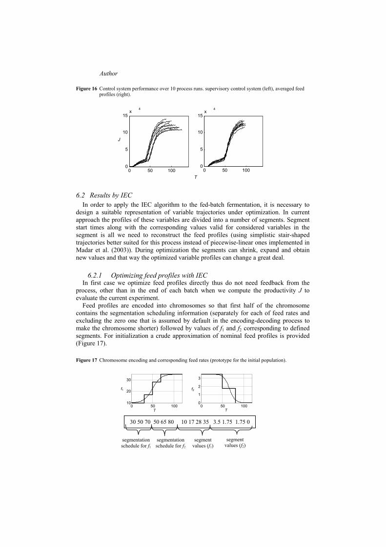
Author
Figure 16 Control system performance over 10 process runs supervisory control system (left) averaged feed profiles (right)
62 Results by IEC In order to apply the IEC algorithm to the fed-batch fermentation it is necessary to
design a suitable representation of variable trajectories under optimization In current approach the profiles of these variables are divided into a number of segments Segment start times along with the corresponding values valid for considered variables in the segment is all we need to reconstruct the feed profiles (using simplistic stair-shaped trajectories better suited for this process instead of piecewise-linear ones implemented in Madar et al (2003)) During optimization the segments can shrink expand and obtain new values and that way the optimized variable profiles can change a great deal
621 Optimizing feed profiles with IEC In first case we optimize feed profiles directly thus do not need feedback from the
process other than in the end of each batch when we compute the productivity J to evaluate the current experiment
Feed profiles are encoded into chromosomes so that first half of the chromosome contains the segmentation scheduling information (separately for each of feed rates and excluding the zero one that is assumed by default in the encoding-decoding process to make the chromosome shorter) followed by values of f1 and f2 corresponding to defined segments For initialization a crude approximation of nominal feed profiles is provided (Figure 17)
Figure 17 Chromosome encoding and corresponding feed rates (prototype for the initial population)
0 50 1000
5
10
15x 4
0 50 1000
5
10
15x
4
T
J
0 50 10010
20
30
0 50 1000
1
2
3
30 50 70 50 65 80 10 17 28 35 35 175 175 0
segmentation schedule for f1
segmentation schedule for f2
segment values (f1)
segment values (f2)
f1 f2
T T
Title
To make up the stochastic nature of both the process and the optimization algorithm we conduct 5 separate optimization cycles The number of individuals in the population is 8 and the number of generations in each series is 20
For the selection procedure we have adopted the following strategy up to four best solutions of the generation are chosen as the parents for the next generation Generally the best one of these is paired with all others and second and third best ones are coupled as well In result the population in each generation contains 4 best solutions of the previous generation and 4 offsprings Note that due to noise the productivity measure alone may be slightly misleading at times because it can vary quite a bit for same feed profiles This is where visualization of all process variables is particularly helpful
Table 5 shows the final results (two best solutions per series) that outperform nominal productivity by 39-66 The learning curve is very smooth (Figure 18) and barely any of the offsprings shows lesser productivity than the nominal feed profiles Therefore the financial cost of the approach is kept minimal
It is possible to use a finer resolution ie a larger number of segments However this would make the search less convergent because of expanded search space and may not pay off in the end
Having a look at the optimized feed profiles (Figure 19) we can conclude that the process is a rather robust one because apparently quite different feed profiles yield similar results Table 5 Productivity of optimized feed profiles
Series no Best solution (J) Second best solution 1 13652sdot105 13372sdot105 2 11530sdot105 11457sdot105 3 13332sdot105 13242sdot105 4 12087sdot105 11580sdot105 5 12530sdot105 11709sdot105
Figure 18 Best solution of the population (105) of five optimization cycles
0 1 2
0 1 2
0 1 2 0 1 2
8 10 12 14 16 18 202 4 60 1 2
No of generations
J
Author
Figure 19 A selection of optimized feed profiles
622 Optimizing substrate concentrations with IEC Taking a step further and optimizing the substrate concentration profiles of s1 and s2 in
the fermenter by EC we no longer need x for scheduling (as in the scheme depicted in Figure 11) On the other hand we still need to measure substrate concentrations online
As with feed profiles optimization a crude approximation of setpoint trajectories from nominal substrate profiles was created that serves as the prototype for the initial population (Figure 20) Table 6 contains the results of optimization (two best solution per series are given) Figure 20 Chromosome encoding for substrate profile optimization and the prototype for initial population
Table 6 Optimization results (second series)
Series no Best solution (J) Second best solution 1 16465sdot105 16213sdot105 2 17016sdot105 16259sdot105 3 17496sdot105 14333sdot105 4 16934sdot105 15662sdot105 5 16924sdot105 16651sdot105
We can observe very strong performance improvement as nominal feed profiles are
now outperformed by 75-113 (this is also better than currently known best result for that process obtained in Liang and Chen (2003))
Compared to the previous optimization scenario the learning process is much more hectic and many potential solutions are subpar This is visualized in Figure 21 that brings
0 20 40 60 800
20
40
T
f1f2
0 20 40 60 800
20
40
T
f1 f2
0 20 40 60 800
20
40
T
f1f2
0 20 40 60 800
20
40
T
f1 f2
20 40 60 80 1000
10 20 30
20 40 60 80 1000
05
115
s1 s2
25 55 70 15 60 80 30 02 03 04 1 005 003 0 0
segmentation schedule for s1
segmentation schedule for s2
segment values (s1)
segment values (s2)
T
Title
out the productivity value of the best offspring in the generation Apparently optimization of s1 and s2 hits the sensitive spot of the process This however is somewhat compensated by faster convergence
Figure 21 Productivity (105) of the fittest offsping in the population (five optimization cycles)
Let us have a closer look what really happens in the fermenter with one of the best yet the simplest substrate profiles (Figure 22) It can be seen that the prescribed value of s1 is achieved rather quickly compared to s2 At around T = 23 the setpoint for s2 becomes equal to zero This moment also marks the beginning of rapid biomass growth which quickly reduces s1 in the fermenter despite that f1 is full on As soon as s2 actually reaches zero biomass growth slows down and rapid product growth starts The latter slows down even before than f1 is considerably reduced and continues to grow with moderate pace till the fermenter volume limit is reached that ends the process Similar process flow can be observed with suboptimal controllers the difference is that with the optimal feedsubstrate profiles everything happens very quickly as the feed rates are quite high throughout the batch
A familiar problem characteristic to the supervisory control scheme is that the variance of results is quite high As before we may use averaged feed profiles of 5 best process runs of tested 10 computed by PI controllers in the control system (Figure 11) that while reducing the average productivity from 169105 to 163105 lead to much more consistent results (Figure 23)
7 Conclusions The properties of the fed-batch fermentation benchmark that resemble real-life
characteristics - presence of noise random variations of state variables parameter drift and ultimately the MIMO nature of the process - make it very difficult to be controlled by traditional means The fact that the orthodox optimal control approach taken in Becerra and Roberts (1998) yields only moderately successful results is a case in point Approximate techniques endorsed by computational intelligence paradigm on the other
1 2 3 4 5 6 7 8 9 100
1
2J
0
1 2
1
15
2
No of generations
1 2 3 4 5 6 7 8 9 100
1
21 2 3 4 5 6 7 8 9 10
0
1
2
1 2 3 4 5 6 7 8 9 10
1 2 3 4 5 6 7 8 9 10
Author
hand are more flexible and as our experiments show also more efficient in information analysis or knowledge acquisition particularly when we are able to properly choose the variable profiles which are going to be optimized (ie optimization of substrate concentrations instead of perhaps more obvious choice of feed rate optimization) that in the end leads to much improved control performance (Figure 24)
Figure 22 Fermentation process with computed setpoint profiles Above product (bold line) and biomass
(normal line) concentrations In the middle Set profiles (slashed lines) vs actual substrate concentrations Below Feed rates 1 (bold line) and 2 (normal line)
Figure 23 Results by IEC before and after averaging the feed profiles
The main challenge with many industrial processes is that even if what we need to
10 20 30 40 50 600
1000
2000 3000
10 20 30 40 50 600
10
20
30
40
0
20
40
20
40
60
0
xp
s1s2
f1f2
10 20 30 40 60T
r2 r1
f1 f2
10 20 30 40 500
05
1
15
2x10
5
10 20 30 40 500
20
40
T T
J
10 20 30 40 50 60 700
05 1
15 2
x10 5
Title
know may be quite simple it is very hard to discover or to learn it in the first place The fed-batch fermentation serves as an adequate example of this situation because even two-segment feed profiles would be sufficient for good performance as Figure 25 amply demonstrates But the discovery that the solution turns out to be simple is just an afterthought in present case
Figure 24 Productivity vs process duration Comparison - results by linguistic inversion (with different
values of p21 which are indicated in the figure) ndash IEC1 - IEC2 - LC1 - LC2 + - DISOPE loz ndash MOC1 diams - MOC2 x - nominal feed profiles
Figure 25 A selection of optimized substrate concentrations
The computational intelligence techniques presented in current paper have both their
advantages and disadvantages For example the linguistic inversion technique that has its advantage for making the design process very transparent is designed so that it aims at maximization of product concentration rather than J and it is therefore more difficult to influence the general dynamics of the process (ie its duration) The latter problem may be a matter of further research
Evolutionary computation on the other hand is more efficient in maximizing J as it searches solution space exhaustively However its computational (and financial) cost may become inhibitive for certain applications
50 100 15005
1
15
2x 10 5
T
J
x
002
05075
15 10
125
10 30T
40T
0 20 400
20 40
T
r1r2
0 20 40 600
20
40
T
r1r2
0 20 400
20 40
r1 r2
0 20 600
20
40
r1r2
Author
References Babuška R (1998) Fuzzy Modeling for Control Kluwer Academic Publishers Boston Baranyi P Bavelaar IM Babuška R Koacuteczy LT Titli A and Verbruggen HB (1998) lsquoA
method to invert a linguistic fuzzy modelrsquo Int J Systems Science Vol 29 No 7 pp711-721 Becerra V M and Roberts P D (1998) lsquoApplication of a novel optimal control algorithm to a
benchmark fed-batch fermentation processrsquoTrans Inst MC Vol 20 No 1 pp11-18 Braae M and Rutherford DA (1979) lsquoTheoretical and Linguistic Aspects of the Fuzzy Logic
Controllerrsquo Automatica Vol 15 No 5 pp553-577 Broyden CG (1965) lsquoA class of methods for solving nonlinear simultaneous equationsrsquo Math
Comp Vol 19 pp577ndash593 Fantuzzi C (1994) lsquoLinguistic rule synthesis of A fuzzy logic controllerrsquo ProcIECON94 pp
1354-1358 Hewitt CJ and Nienow AW (2007) lsquoThe scale-up of microbial batch and fed-batch
fermentation processesrsquo Adv Appl Microbiol Vol 62 pp105-135 Holland JH (1975) Adaptation in natural and artificial systems The University of Michigan
Press Ann Arbor Holmblad LP and Ostergaard J-J lsquoControl of a cement kiln by fuzzy logicrsquo in Gupta MM and
Sanchez E (1982) Fuzzy Information and Decision Processes North-Holland Publishing Company Amsterdam pp389ndash399
Hough P D Kolda T G and Torczon V J (2001) lsquoAsynchronous parallel pattern search for nonlinear optimizationrsquo SIAM J Sci Comput Vol 23 pp134ndash156
Kawohl M Heine T and King R (2007) lsquoModel based estimation and optimal control of fed-batch fermentation processes for the production of antibioticsrsquo Chemical engineering and processing Vol 46 No 11 pp1223-1241
Jang J-S R Sun C-T and Mizutani E (1996) Neuro-Fuzzy and Soft Computing A Computational Approach to Learning and Machine Intelligence Prentice Hall Upper Saddle River
Jensen CA Reed RD Marks RJ El-Sharkawi MA Jung J-B Miyamoto RT Anderson GM and Eggen CJ (1999) lsquoInversion of feedforward neural networks Algorithms and applicationsrsquo Proceedings of the IEEE Vol 87 No 9 pp1536-1549
Leigh R (1998) lsquoFed-batch fermentation process modelling and control competitionrsquo Trans Inst MC Vol 20 No 1 p3
Liang J and Chen Y (2003) lsquoOptimization of a fed-batch fermentation process control competition problem using the NEOS serverrsquo Proc Inst Mech Engrs Part I J Systems Control Eng Vol 217 Part 5 pp427-432
Liang J Chen Y Meng MQ-H and Fullmer R (2003) lsquoSolving Tough Optimal Control Problem by Network Enabled Optimization Server (NEOS)rsquo Proc IEEE Intelligent Automation Conf
Lotfi A Andersen H C and Tsoi A C (1996) lsquoInterpretation Preservation of Adaptive Fuzzy Inference Systemsrsquo Int J Approximate Reasoning Vol 15 No 4 pp379-394
Ma Y (2007) lsquoResearch on On-Line Modeling of Fed-Batch Fermentation Process Based on v-SVRrsquo in Huang D-S Heutte L and Loog M (eds) Advanced Intelligent Computing Theories and ApplicationsWith Aspects of Artificial Intelligence Springer pp900-908
Madaacuter J Abonyi J and Szeifert F (2003) lsquoInteractive Evolutionary Computation for model based Optimization of Batch Fermentationrsquo IASTED International Conference on Artificial Intelligence and Applications Benalmaacutedena Spain pp100-105
Mayer DG Belward JA Widell H and Burrage K (1999) lsquoSurvival of the fittestmdash algorithms versus evolution strategies in the optimization of systems modelsrsquo Agricultural Systems Vol 60 No 2 pp113-122
Title
McKay B Sanderson CS Willis MJ Bartford JP and Barton GW (1998) lsquoEvolving a hybrid model of a fed-batch fermentation processrsquo Trans Inst MC Vol 20 No 1 pp4-10
Nomikos P and MacGregor JF (1994) lsquoMonitoring batch processes using multiway principal component analysisrsquo AIChe Journal Vol 40 pp1361-75
Nozaki K Ishibuchi H and Tanaka H (1997) lsquoA simple but powerful heuristic method for generating fuzzy rules from numerical datarsquo Fuzzy Sets and Systems Vol 86 No 3 pp251-270
de Oliveira JV (1999) lsquoSemantic constraints for membership function optimizationrsquo IEEE Trans Systems Man and Cybernetics Vol 29 No 1 pp128 -138
Pedrycz W (editor) (1997) Fuzzy Evolutionary Computation Kluwer Aademic Publishers New York
Raymond C Boverie S and Titli A (1995) lsquoFuzzy multivariable control design from the fuzzy system modelrsquo Proc IFSA World Congr pp509-511
Rechenberg I (1973) Evolutionsstrategie - Optimierung technischer Systeme nach Prinzipien der biologischen Evolution Frommann-Holzboog Stuttgart
Riid A and E Ruumlstern E (2000a) lsquoSupervisory fed-batch fermentation control on the basis of linguistically interpretable fuzzy modelsrsquo Proc Estonian Acad Sci Eng Vol 6 No 2 pp96-112
Riid A and E Ruumlstern E (2000b) lsquoTransparent fuzzy systems and modeling with transparency protectionrsquo Proc IFAC Symp on Artificial Intelligence in Real Time Control pp229-234
Riid A and Ruumlstern E (2003) lsquoTransparent Fuzzy Systems in Modeling and Controlrsquo in Casillas J Cordon O Herrera F and Magdalena L (editors) Interpretability Issues in Fuzzy Modeling Springer pp452-476
Riid A and E Ruumlstern E (2006) lsquoAutomatic Linguistic Inversion of a Fuzzy Model for Fed-Batch Fermentation Controlrsquo Proc10th Int Conf Intelligent Engineering Systems pp129-134
Riid A and E Ruumlstern E (2007) lsquoInterpretability of Fuzzy Systems and Its Application to Process Controlrsquo Proc IEEE Int Conf Fuzzy Systems pp 1-6
Riid A and E Ruumlstern E (2008) lsquoFed-Batch Fermentation Controller Design with Evolutionary Computationrsquo Proc 5th ACMIEEE Int Conf Soft Computing as Transdisciplinary Science and Technology pp371-377
Soufian M and Soufian M (1997) lsquoParallel Genetic Algorithms for Optimised Fuzzy Modelling with application to a Fermentation Processrsquo Proc 2nd Int Conf on Genetic Algorithms In Engineering Systems Innovations and Applications pp123-128
Soufian M Soufian M and Dempsey MJ (1998) lsquoThe Effect of a Dynamical Layer in Neural Network Prediction of Biomass in a Fermentation ProcessrsquoLecture notes in computer science Vol 1415 pp749-757
Takagi T and Sugeno M (1985) lsquoFuzzy identification of systems and its applications to modeling and controlrsquo IEEE Trans Syst Man Cybern Vol SMC-15 No 1 pp116-132
Zhang H and Lennox B (2003) lsquoMulti-way optimal contol of a benchmark fed-batch fermentation processrsquo Trans Inst MC Vol 25 No 5 pp403-417
Zhang H Lennox B Goulding PR and Leung AYT (2000) lsquoA float-encoded genetic algorithm technique for integrated optimization of piezoelectric actuator and sensor placement and feedback gainsrsquo Smart Mater Struct Vol 9 pp552ndash557
Zhang H (2008) lsquoOptimal control of a fed-batch yeast fermentation process based on Least Square Support Vector Machinersquo Int J Engineering Systems Modelling and Simulation Vol 1 No 1 pp63-68

Title
To make up the stochastic nature of both the process and the optimization algorithm we conduct 5 separate optimization cycles The number of individuals in the population is 8 and the number of generations in each series is 20
For the selection procedure we have adopted the following strategy up to four best solutions of the generation are chosen as the parents for the next generation Generally the best one of these is paired with all others and second and third best ones are coupled as well In result the population in each generation contains 4 best solutions of the previous generation and 4 offsprings Note that due to noise the productivity measure alone may be slightly misleading at times because it can vary quite a bit for same feed profiles This is where visualization of all process variables is particularly helpful
Table 5 shows the final results (two best solutions per series) that outperform nominal productivity by 39-66 The learning curve is very smooth (Figure 18) and barely any of the offsprings shows lesser productivity than the nominal feed profiles Therefore the financial cost of the approach is kept minimal
It is possible to use a finer resolution ie a larger number of segments However this would make the search less convergent because of expanded search space and may not pay off in the end
Having a look at the optimized feed profiles (Figure 19) we can conclude that the process is a rather robust one because apparently quite different feed profiles yield similar results Table 5 Productivity of optimized feed profiles
Series no Best solution (J) Second best solution 1 13652sdot105 13372sdot105 2 11530sdot105 11457sdot105 3 13332sdot105 13242sdot105 4 12087sdot105 11580sdot105 5 12530sdot105 11709sdot105
Figure 18 Best solution of the population (105) of five optimization cycles
0 1 2
0 1 2
0 1 2 0 1 2
8 10 12 14 16 18 202 4 60 1 2
No of generations
J
Author
Figure 19 A selection of optimized feed profiles
622 Optimizing substrate concentrations with IEC Taking a step further and optimizing the substrate concentration profiles of s1 and s2 in
the fermenter by EC we no longer need x for scheduling (as in the scheme depicted in Figure 11) On the other hand we still need to measure substrate concentrations online
As with feed profiles optimization a crude approximation of setpoint trajectories from nominal substrate profiles was created that serves as the prototype for the initial population (Figure 20) Table 6 contains the results of optimization (two best solution per series are given) Figure 20 Chromosome encoding for substrate profile optimization and the prototype for initial population
Table 6 Optimization results (second series)
Series no Best solution (J) Second best solution 1 16465sdot105 16213sdot105 2 17016sdot105 16259sdot105 3 17496sdot105 14333sdot105 4 16934sdot105 15662sdot105 5 16924sdot105 16651sdot105
We can observe very strong performance improvement as nominal feed profiles are
now outperformed by 75-113 (this is also better than currently known best result for that process obtained in Liang and Chen (2003))
Compared to the previous optimization scenario the learning process is much more hectic and many potential solutions are subpar This is visualized in Figure 21 that brings
0 20 40 60 800
20
40
T
f1f2
0 20 40 60 800
20
40
T
f1 f2
0 20 40 60 800
20
40
T
f1f2
0 20 40 60 800
20
40
T
f1 f2
20 40 60 80 1000
10 20 30
20 40 60 80 1000
05
115
s1 s2
25 55 70 15 60 80 30 02 03 04 1 005 003 0 0
segmentation schedule for s1
segmentation schedule for s2
segment values (s1)
segment values (s2)
T
Title
out the productivity value of the best offspring in the generation Apparently optimization of s1 and s2 hits the sensitive spot of the process This however is somewhat compensated by faster convergence
Figure 21 Productivity (105) of the fittest offsping in the population (five optimization cycles)
Let us have a closer look what really happens in the fermenter with one of the best yet the simplest substrate profiles (Figure 22) It can be seen that the prescribed value of s1 is achieved rather quickly compared to s2 At around T = 23 the setpoint for s2 becomes equal to zero This moment also marks the beginning of rapid biomass growth which quickly reduces s1 in the fermenter despite that f1 is full on As soon as s2 actually reaches zero biomass growth slows down and rapid product growth starts The latter slows down even before than f1 is considerably reduced and continues to grow with moderate pace till the fermenter volume limit is reached that ends the process Similar process flow can be observed with suboptimal controllers the difference is that with the optimal feedsubstrate profiles everything happens very quickly as the feed rates are quite high throughout the batch
A familiar problem characteristic to the supervisory control scheme is that the variance of results is quite high As before we may use averaged feed profiles of 5 best process runs of tested 10 computed by PI controllers in the control system (Figure 11) that while reducing the average productivity from 169105 to 163105 lead to much more consistent results (Figure 23)
7 Conclusions The properties of the fed-batch fermentation benchmark that resemble real-life
characteristics - presence of noise random variations of state variables parameter drift and ultimately the MIMO nature of the process - make it very difficult to be controlled by traditional means The fact that the orthodox optimal control approach taken in Becerra and Roberts (1998) yields only moderately successful results is a case in point Approximate techniques endorsed by computational intelligence paradigm on the other
1 2 3 4 5 6 7 8 9 100
1
2J
0
1 2
1
15
2
No of generations
1 2 3 4 5 6 7 8 9 100
1
21 2 3 4 5 6 7 8 9 10
0
1
2
1 2 3 4 5 6 7 8 9 10
1 2 3 4 5 6 7 8 9 10
Author
hand are more flexible and as our experiments show also more efficient in information analysis or knowledge acquisition particularly when we are able to properly choose the variable profiles which are going to be optimized (ie optimization of substrate concentrations instead of perhaps more obvious choice of feed rate optimization) that in the end leads to much improved control performance (Figure 24)
Figure 22 Fermentation process with computed setpoint profiles Above product (bold line) and biomass
(normal line) concentrations In the middle Set profiles (slashed lines) vs actual substrate concentrations Below Feed rates 1 (bold line) and 2 (normal line)
Figure 23 Results by IEC before and after averaging the feed profiles
The main challenge with many industrial processes is that even if what we need to
10 20 30 40 50 600
1000
2000 3000
10 20 30 40 50 600
10
20
30
40
0
20
40
20
40
60
0
xp
s1s2
f1f2
10 20 30 40 60T
r2 r1
f1 f2
10 20 30 40 500
05
1
15
2x10
5
10 20 30 40 500
20
40
T T
J
10 20 30 40 50 60 700
05 1
15 2
x10 5
Title
know may be quite simple it is very hard to discover or to learn it in the first place The fed-batch fermentation serves as an adequate example of this situation because even two-segment feed profiles would be sufficient for good performance as Figure 25 amply demonstrates But the discovery that the solution turns out to be simple is just an afterthought in present case
Figure 24 Productivity vs process duration Comparison - results by linguistic inversion (with different
values of p21 which are indicated in the figure) ndash IEC1 - IEC2 - LC1 - LC2 + - DISOPE loz ndash MOC1 diams - MOC2 x - nominal feed profiles
Figure 25 A selection of optimized substrate concentrations
The computational intelligence techniques presented in current paper have both their
advantages and disadvantages For example the linguistic inversion technique that has its advantage for making the design process very transparent is designed so that it aims at maximization of product concentration rather than J and it is therefore more difficult to influence the general dynamics of the process (ie its duration) The latter problem may be a matter of further research
Evolutionary computation on the other hand is more efficient in maximizing J as it searches solution space exhaustively However its computational (and financial) cost may become inhibitive for certain applications
50 100 15005
1
15
2x 10 5
T
J
x
002
05075
15 10
125
10 30T
40T
0 20 400
20 40
T
r1r2
0 20 40 600
20
40
T
r1r2
0 20 400
20 40
r1 r2
0 20 600
20
40
r1r2
Author
References Babuška R (1998) Fuzzy Modeling for Control Kluwer Academic Publishers Boston Baranyi P Bavelaar IM Babuška R Koacuteczy LT Titli A and Verbruggen HB (1998) lsquoA
method to invert a linguistic fuzzy modelrsquo Int J Systems Science Vol 29 No 7 pp711-721 Becerra V M and Roberts P D (1998) lsquoApplication of a novel optimal control algorithm to a
benchmark fed-batch fermentation processrsquoTrans Inst MC Vol 20 No 1 pp11-18 Braae M and Rutherford DA (1979) lsquoTheoretical and Linguistic Aspects of the Fuzzy Logic
Controllerrsquo Automatica Vol 15 No 5 pp553-577 Broyden CG (1965) lsquoA class of methods for solving nonlinear simultaneous equationsrsquo Math
Comp Vol 19 pp577ndash593 Fantuzzi C (1994) lsquoLinguistic rule synthesis of A fuzzy logic controllerrsquo ProcIECON94 pp
1354-1358 Hewitt CJ and Nienow AW (2007) lsquoThe scale-up of microbial batch and fed-batch
fermentation processesrsquo Adv Appl Microbiol Vol 62 pp105-135 Holland JH (1975) Adaptation in natural and artificial systems The University of Michigan
Press Ann Arbor Holmblad LP and Ostergaard J-J lsquoControl of a cement kiln by fuzzy logicrsquo in Gupta MM and
Sanchez E (1982) Fuzzy Information and Decision Processes North-Holland Publishing Company Amsterdam pp389ndash399
Hough P D Kolda T G and Torczon V J (2001) lsquoAsynchronous parallel pattern search for nonlinear optimizationrsquo SIAM J Sci Comput Vol 23 pp134ndash156
Kawohl M Heine T and King R (2007) lsquoModel based estimation and optimal control of fed-batch fermentation processes for the production of antibioticsrsquo Chemical engineering and processing Vol 46 No 11 pp1223-1241
Jang J-S R Sun C-T and Mizutani E (1996) Neuro-Fuzzy and Soft Computing A Computational Approach to Learning and Machine Intelligence Prentice Hall Upper Saddle River
Jensen CA Reed RD Marks RJ El-Sharkawi MA Jung J-B Miyamoto RT Anderson GM and Eggen CJ (1999) lsquoInversion of feedforward neural networks Algorithms and applicationsrsquo Proceedings of the IEEE Vol 87 No 9 pp1536-1549
Leigh R (1998) lsquoFed-batch fermentation process modelling and control competitionrsquo Trans Inst MC Vol 20 No 1 p3
Liang J and Chen Y (2003) lsquoOptimization of a fed-batch fermentation process control competition problem using the NEOS serverrsquo Proc Inst Mech Engrs Part I J Systems Control Eng Vol 217 Part 5 pp427-432
Liang J Chen Y Meng MQ-H and Fullmer R (2003) lsquoSolving Tough Optimal Control Problem by Network Enabled Optimization Server (NEOS)rsquo Proc IEEE Intelligent Automation Conf
Lotfi A Andersen H C and Tsoi A C (1996) lsquoInterpretation Preservation of Adaptive Fuzzy Inference Systemsrsquo Int J Approximate Reasoning Vol 15 No 4 pp379-394
Ma Y (2007) lsquoResearch on On-Line Modeling of Fed-Batch Fermentation Process Based on v-SVRrsquo in Huang D-S Heutte L and Loog M (eds) Advanced Intelligent Computing Theories and ApplicationsWith Aspects of Artificial Intelligence Springer pp900-908
Madaacuter J Abonyi J and Szeifert F (2003) lsquoInteractive Evolutionary Computation for model based Optimization of Batch Fermentationrsquo IASTED International Conference on Artificial Intelligence and Applications Benalmaacutedena Spain pp100-105
Mayer DG Belward JA Widell H and Burrage K (1999) lsquoSurvival of the fittestmdash algorithms versus evolution strategies in the optimization of systems modelsrsquo Agricultural Systems Vol 60 No 2 pp113-122
Title
McKay B Sanderson CS Willis MJ Bartford JP and Barton GW (1998) lsquoEvolving a hybrid model of a fed-batch fermentation processrsquo Trans Inst MC Vol 20 No 1 pp4-10
Nomikos P and MacGregor JF (1994) lsquoMonitoring batch processes using multiway principal component analysisrsquo AIChe Journal Vol 40 pp1361-75
Nozaki K Ishibuchi H and Tanaka H (1997) lsquoA simple but powerful heuristic method for generating fuzzy rules from numerical datarsquo Fuzzy Sets and Systems Vol 86 No 3 pp251-270
de Oliveira JV (1999) lsquoSemantic constraints for membership function optimizationrsquo IEEE Trans Systems Man and Cybernetics Vol 29 No 1 pp128 -138
Pedrycz W (editor) (1997) Fuzzy Evolutionary Computation Kluwer Aademic Publishers New York
Raymond C Boverie S and Titli A (1995) lsquoFuzzy multivariable control design from the fuzzy system modelrsquo Proc IFSA World Congr pp509-511
Rechenberg I (1973) Evolutionsstrategie - Optimierung technischer Systeme nach Prinzipien der biologischen Evolution Frommann-Holzboog Stuttgart
Riid A and E Ruumlstern E (2000a) lsquoSupervisory fed-batch fermentation control on the basis of linguistically interpretable fuzzy modelsrsquo Proc Estonian Acad Sci Eng Vol 6 No 2 pp96-112
Riid A and E Ruumlstern E (2000b) lsquoTransparent fuzzy systems and modeling with transparency protectionrsquo Proc IFAC Symp on Artificial Intelligence in Real Time Control pp229-234
Riid A and Ruumlstern E (2003) lsquoTransparent Fuzzy Systems in Modeling and Controlrsquo in Casillas J Cordon O Herrera F and Magdalena L (editors) Interpretability Issues in Fuzzy Modeling Springer pp452-476
Riid A and E Ruumlstern E (2006) lsquoAutomatic Linguistic Inversion of a Fuzzy Model for Fed-Batch Fermentation Controlrsquo Proc10th Int Conf Intelligent Engineering Systems pp129-134
Riid A and E Ruumlstern E (2007) lsquoInterpretability of Fuzzy Systems and Its Application to Process Controlrsquo Proc IEEE Int Conf Fuzzy Systems pp 1-6
Riid A and E Ruumlstern E (2008) lsquoFed-Batch Fermentation Controller Design with Evolutionary Computationrsquo Proc 5th ACMIEEE Int Conf Soft Computing as Transdisciplinary Science and Technology pp371-377
Soufian M and Soufian M (1997) lsquoParallel Genetic Algorithms for Optimised Fuzzy Modelling with application to a Fermentation Processrsquo Proc 2nd Int Conf on Genetic Algorithms In Engineering Systems Innovations and Applications pp123-128
Soufian M Soufian M and Dempsey MJ (1998) lsquoThe Effect of a Dynamical Layer in Neural Network Prediction of Biomass in a Fermentation ProcessrsquoLecture notes in computer science Vol 1415 pp749-757
Takagi T and Sugeno M (1985) lsquoFuzzy identification of systems and its applications to modeling and controlrsquo IEEE Trans Syst Man Cybern Vol SMC-15 No 1 pp116-132
Zhang H and Lennox B (2003) lsquoMulti-way optimal contol of a benchmark fed-batch fermentation processrsquo Trans Inst MC Vol 25 No 5 pp403-417
Zhang H Lennox B Goulding PR and Leung AYT (2000) lsquoA float-encoded genetic algorithm technique for integrated optimization of piezoelectric actuator and sensor placement and feedback gainsrsquo Smart Mater Struct Vol 9 pp552ndash557
Zhang H (2008) lsquoOptimal control of a fed-batch yeast fermentation process based on Least Square Support Vector Machinersquo Int J Engineering Systems Modelling and Simulation Vol 1 No 1 pp63-68

Author
Figure 19 A selection of optimized feed profiles
622 Optimizing substrate concentrations with IEC Taking a step further and optimizing the substrate concentration profiles of s1 and s2 in
the fermenter by EC we no longer need x for scheduling (as in the scheme depicted in Figure 11) On the other hand we still need to measure substrate concentrations online
As with feed profiles optimization a crude approximation of setpoint trajectories from nominal substrate profiles was created that serves as the prototype for the initial population (Figure 20) Table 6 contains the results of optimization (two best solution per series are given) Figure 20 Chromosome encoding for substrate profile optimization and the prototype for initial population
Table 6 Optimization results (second series)
Series no Best solution (J) Second best solution 1 16465sdot105 16213sdot105 2 17016sdot105 16259sdot105 3 17496sdot105 14333sdot105 4 16934sdot105 15662sdot105 5 16924sdot105 16651sdot105
We can observe very strong performance improvement as nominal feed profiles are
now outperformed by 75-113 (this is also better than currently known best result for that process obtained in Liang and Chen (2003))
Compared to the previous optimization scenario the learning process is much more hectic and many potential solutions are subpar This is visualized in Figure 21 that brings
0 20 40 60 800
20
40
T
f1f2
0 20 40 60 800
20
40
T
f1 f2
0 20 40 60 800
20
40
T
f1f2
0 20 40 60 800
20
40
T
f1 f2
20 40 60 80 1000
10 20 30
20 40 60 80 1000
05
115
s1 s2
25 55 70 15 60 80 30 02 03 04 1 005 003 0 0
segmentation schedule for s1
segmentation schedule for s2
segment values (s1)
segment values (s2)
T
Title
out the productivity value of the best offspring in the generation Apparently optimization of s1 and s2 hits the sensitive spot of the process This however is somewhat compensated by faster convergence
Figure 21 Productivity (105) of the fittest offsping in the population (five optimization cycles)
Let us have a closer look what really happens in the fermenter with one of the best yet the simplest substrate profiles (Figure 22) It can be seen that the prescribed value of s1 is achieved rather quickly compared to s2 At around T = 23 the setpoint for s2 becomes equal to zero This moment also marks the beginning of rapid biomass growth which quickly reduces s1 in the fermenter despite that f1 is full on As soon as s2 actually reaches zero biomass growth slows down and rapid product growth starts The latter slows down even before than f1 is considerably reduced and continues to grow with moderate pace till the fermenter volume limit is reached that ends the process Similar process flow can be observed with suboptimal controllers the difference is that with the optimal feedsubstrate profiles everything happens very quickly as the feed rates are quite high throughout the batch
A familiar problem characteristic to the supervisory control scheme is that the variance of results is quite high As before we may use averaged feed profiles of 5 best process runs of tested 10 computed by PI controllers in the control system (Figure 11) that while reducing the average productivity from 169105 to 163105 lead to much more consistent results (Figure 23)
7 Conclusions The properties of the fed-batch fermentation benchmark that resemble real-life
characteristics - presence of noise random variations of state variables parameter drift and ultimately the MIMO nature of the process - make it very difficult to be controlled by traditional means The fact that the orthodox optimal control approach taken in Becerra and Roberts (1998) yields only moderately successful results is a case in point Approximate techniques endorsed by computational intelligence paradigm on the other
1 2 3 4 5 6 7 8 9 100
1
2J
0
1 2
1
15
2
No of generations
1 2 3 4 5 6 7 8 9 100
1
21 2 3 4 5 6 7 8 9 10
0
1
2
1 2 3 4 5 6 7 8 9 10
1 2 3 4 5 6 7 8 9 10
Author
hand are more flexible and as our experiments show also more efficient in information analysis or knowledge acquisition particularly when we are able to properly choose the variable profiles which are going to be optimized (ie optimization of substrate concentrations instead of perhaps more obvious choice of feed rate optimization) that in the end leads to much improved control performance (Figure 24)
Figure 22 Fermentation process with computed setpoint profiles Above product (bold line) and biomass
(normal line) concentrations In the middle Set profiles (slashed lines) vs actual substrate concentrations Below Feed rates 1 (bold line) and 2 (normal line)
Figure 23 Results by IEC before and after averaging the feed profiles
The main challenge with many industrial processes is that even if what we need to
10 20 30 40 50 600
1000
2000 3000
10 20 30 40 50 600
10
20
30
40
0
20
40
20
40
60
0
xp
s1s2
f1f2
10 20 30 40 60T
r2 r1
f1 f2
10 20 30 40 500
05
1
15
2x10
5
10 20 30 40 500
20
40
T T
J
10 20 30 40 50 60 700
05 1
15 2
x10 5
Title
know may be quite simple it is very hard to discover or to learn it in the first place The fed-batch fermentation serves as an adequate example of this situation because even two-segment feed profiles would be sufficient for good performance as Figure 25 amply demonstrates But the discovery that the solution turns out to be simple is just an afterthought in present case
Figure 24 Productivity vs process duration Comparison - results by linguistic inversion (with different
values of p21 which are indicated in the figure) ndash IEC1 - IEC2 - LC1 - LC2 + - DISOPE loz ndash MOC1 diams - MOC2 x - nominal feed profiles
Figure 25 A selection of optimized substrate concentrations
The computational intelligence techniques presented in current paper have both their
advantages and disadvantages For example the linguistic inversion technique that has its advantage for making the design process very transparent is designed so that it aims at maximization of product concentration rather than J and it is therefore more difficult to influence the general dynamics of the process (ie its duration) The latter problem may be a matter of further research
Evolutionary computation on the other hand is more efficient in maximizing J as it searches solution space exhaustively However its computational (and financial) cost may become inhibitive for certain applications
50 100 15005
1
15
2x 10 5
T
J
x
002
05075
15 10
125
10 30T
40T
0 20 400
20 40
T
r1r2
0 20 40 600
20
40
T
r1r2
0 20 400
20 40
r1 r2
0 20 600
20
40
r1r2
Author
References Babuška R (1998) Fuzzy Modeling for Control Kluwer Academic Publishers Boston Baranyi P Bavelaar IM Babuška R Koacuteczy LT Titli A and Verbruggen HB (1998) lsquoA
method to invert a linguistic fuzzy modelrsquo Int J Systems Science Vol 29 No 7 pp711-721 Becerra V M and Roberts P D (1998) lsquoApplication of a novel optimal control algorithm to a
benchmark fed-batch fermentation processrsquoTrans Inst MC Vol 20 No 1 pp11-18 Braae M and Rutherford DA (1979) lsquoTheoretical and Linguistic Aspects of the Fuzzy Logic
Controllerrsquo Automatica Vol 15 No 5 pp553-577 Broyden CG (1965) lsquoA class of methods for solving nonlinear simultaneous equationsrsquo Math
Comp Vol 19 pp577ndash593 Fantuzzi C (1994) lsquoLinguistic rule synthesis of A fuzzy logic controllerrsquo ProcIECON94 pp
1354-1358 Hewitt CJ and Nienow AW (2007) lsquoThe scale-up of microbial batch and fed-batch
fermentation processesrsquo Adv Appl Microbiol Vol 62 pp105-135 Holland JH (1975) Adaptation in natural and artificial systems The University of Michigan
Press Ann Arbor Holmblad LP and Ostergaard J-J lsquoControl of a cement kiln by fuzzy logicrsquo in Gupta MM and
Sanchez E (1982) Fuzzy Information and Decision Processes North-Holland Publishing Company Amsterdam pp389ndash399
Hough P D Kolda T G and Torczon V J (2001) lsquoAsynchronous parallel pattern search for nonlinear optimizationrsquo SIAM J Sci Comput Vol 23 pp134ndash156
Kawohl M Heine T and King R (2007) lsquoModel based estimation and optimal control of fed-batch fermentation processes for the production of antibioticsrsquo Chemical engineering and processing Vol 46 No 11 pp1223-1241
Jang J-S R Sun C-T and Mizutani E (1996) Neuro-Fuzzy and Soft Computing A Computational Approach to Learning and Machine Intelligence Prentice Hall Upper Saddle River
Jensen CA Reed RD Marks RJ El-Sharkawi MA Jung J-B Miyamoto RT Anderson GM and Eggen CJ (1999) lsquoInversion of feedforward neural networks Algorithms and applicationsrsquo Proceedings of the IEEE Vol 87 No 9 pp1536-1549
Leigh R (1998) lsquoFed-batch fermentation process modelling and control competitionrsquo Trans Inst MC Vol 20 No 1 p3
Liang J and Chen Y (2003) lsquoOptimization of a fed-batch fermentation process control competition problem using the NEOS serverrsquo Proc Inst Mech Engrs Part I J Systems Control Eng Vol 217 Part 5 pp427-432
Liang J Chen Y Meng MQ-H and Fullmer R (2003) lsquoSolving Tough Optimal Control Problem by Network Enabled Optimization Server (NEOS)rsquo Proc IEEE Intelligent Automation Conf
Lotfi A Andersen H C and Tsoi A C (1996) lsquoInterpretation Preservation of Adaptive Fuzzy Inference Systemsrsquo Int J Approximate Reasoning Vol 15 No 4 pp379-394
Ma Y (2007) lsquoResearch on On-Line Modeling of Fed-Batch Fermentation Process Based on v-SVRrsquo in Huang D-S Heutte L and Loog M (eds) Advanced Intelligent Computing Theories and ApplicationsWith Aspects of Artificial Intelligence Springer pp900-908
Madaacuter J Abonyi J and Szeifert F (2003) lsquoInteractive Evolutionary Computation for model based Optimization of Batch Fermentationrsquo IASTED International Conference on Artificial Intelligence and Applications Benalmaacutedena Spain pp100-105
Mayer DG Belward JA Widell H and Burrage K (1999) lsquoSurvival of the fittestmdash algorithms versus evolution strategies in the optimization of systems modelsrsquo Agricultural Systems Vol 60 No 2 pp113-122
Title
McKay B Sanderson CS Willis MJ Bartford JP and Barton GW (1998) lsquoEvolving a hybrid model of a fed-batch fermentation processrsquo Trans Inst MC Vol 20 No 1 pp4-10
Nomikos P and MacGregor JF (1994) lsquoMonitoring batch processes using multiway principal component analysisrsquo AIChe Journal Vol 40 pp1361-75
Nozaki K Ishibuchi H and Tanaka H (1997) lsquoA simple but powerful heuristic method for generating fuzzy rules from numerical datarsquo Fuzzy Sets and Systems Vol 86 No 3 pp251-270
de Oliveira JV (1999) lsquoSemantic constraints for membership function optimizationrsquo IEEE Trans Systems Man and Cybernetics Vol 29 No 1 pp128 -138
Pedrycz W (editor) (1997) Fuzzy Evolutionary Computation Kluwer Aademic Publishers New York
Raymond C Boverie S and Titli A (1995) lsquoFuzzy multivariable control design from the fuzzy system modelrsquo Proc IFSA World Congr pp509-511
Rechenberg I (1973) Evolutionsstrategie - Optimierung technischer Systeme nach Prinzipien der biologischen Evolution Frommann-Holzboog Stuttgart
Riid A and E Ruumlstern E (2000a) lsquoSupervisory fed-batch fermentation control on the basis of linguistically interpretable fuzzy modelsrsquo Proc Estonian Acad Sci Eng Vol 6 No 2 pp96-112
Riid A and E Ruumlstern E (2000b) lsquoTransparent fuzzy systems and modeling with transparency protectionrsquo Proc IFAC Symp on Artificial Intelligence in Real Time Control pp229-234
Riid A and Ruumlstern E (2003) lsquoTransparent Fuzzy Systems in Modeling and Controlrsquo in Casillas J Cordon O Herrera F and Magdalena L (editors) Interpretability Issues in Fuzzy Modeling Springer pp452-476
Riid A and E Ruumlstern E (2006) lsquoAutomatic Linguistic Inversion of a Fuzzy Model for Fed-Batch Fermentation Controlrsquo Proc10th Int Conf Intelligent Engineering Systems pp129-134
Riid A and E Ruumlstern E (2007) lsquoInterpretability of Fuzzy Systems and Its Application to Process Controlrsquo Proc IEEE Int Conf Fuzzy Systems pp 1-6
Riid A and E Ruumlstern E (2008) lsquoFed-Batch Fermentation Controller Design with Evolutionary Computationrsquo Proc 5th ACMIEEE Int Conf Soft Computing as Transdisciplinary Science and Technology pp371-377
Soufian M and Soufian M (1997) lsquoParallel Genetic Algorithms for Optimised Fuzzy Modelling with application to a Fermentation Processrsquo Proc 2nd Int Conf on Genetic Algorithms In Engineering Systems Innovations and Applications pp123-128
Soufian M Soufian M and Dempsey MJ (1998) lsquoThe Effect of a Dynamical Layer in Neural Network Prediction of Biomass in a Fermentation ProcessrsquoLecture notes in computer science Vol 1415 pp749-757
Takagi T and Sugeno M (1985) lsquoFuzzy identification of systems and its applications to modeling and controlrsquo IEEE Trans Syst Man Cybern Vol SMC-15 No 1 pp116-132
Zhang H and Lennox B (2003) lsquoMulti-way optimal contol of a benchmark fed-batch fermentation processrsquo Trans Inst MC Vol 25 No 5 pp403-417
Zhang H Lennox B Goulding PR and Leung AYT (2000) lsquoA float-encoded genetic algorithm technique for integrated optimization of piezoelectric actuator and sensor placement and feedback gainsrsquo Smart Mater Struct Vol 9 pp552ndash557
Zhang H (2008) lsquoOptimal control of a fed-batch yeast fermentation process based on Least Square Support Vector Machinersquo Int J Engineering Systems Modelling and Simulation Vol 1 No 1 pp63-68

Title
out the productivity value of the best offspring in the generation Apparently optimization of s1 and s2 hits the sensitive spot of the process This however is somewhat compensated by faster convergence
Figure 21 Productivity (105) of the fittest offsping in the population (five optimization cycles)
Let us have a closer look what really happens in the fermenter with one of the best yet the simplest substrate profiles (Figure 22) It can be seen that the prescribed value of s1 is achieved rather quickly compared to s2 At around T = 23 the setpoint for s2 becomes equal to zero This moment also marks the beginning of rapid biomass growth which quickly reduces s1 in the fermenter despite that f1 is full on As soon as s2 actually reaches zero biomass growth slows down and rapid product growth starts The latter slows down even before than f1 is considerably reduced and continues to grow with moderate pace till the fermenter volume limit is reached that ends the process Similar process flow can be observed with suboptimal controllers the difference is that with the optimal feedsubstrate profiles everything happens very quickly as the feed rates are quite high throughout the batch
A familiar problem characteristic to the supervisory control scheme is that the variance of results is quite high As before we may use averaged feed profiles of 5 best process runs of tested 10 computed by PI controllers in the control system (Figure 11) that while reducing the average productivity from 169105 to 163105 lead to much more consistent results (Figure 23)
7 Conclusions The properties of the fed-batch fermentation benchmark that resemble real-life
characteristics - presence of noise random variations of state variables parameter drift and ultimately the MIMO nature of the process - make it very difficult to be controlled by traditional means The fact that the orthodox optimal control approach taken in Becerra and Roberts (1998) yields only moderately successful results is a case in point Approximate techniques endorsed by computational intelligence paradigm on the other
1 2 3 4 5 6 7 8 9 100
1
2J
0
1 2
1
15
2
No of generations
1 2 3 4 5 6 7 8 9 100
1
21 2 3 4 5 6 7 8 9 10
0
1
2
1 2 3 4 5 6 7 8 9 10
1 2 3 4 5 6 7 8 9 10
Author
hand are more flexible and as our experiments show also more efficient in information analysis or knowledge acquisition particularly when we are able to properly choose the variable profiles which are going to be optimized (ie optimization of substrate concentrations instead of perhaps more obvious choice of feed rate optimization) that in the end leads to much improved control performance (Figure 24)
Figure 22 Fermentation process with computed setpoint profiles Above product (bold line) and biomass
(normal line) concentrations In the middle Set profiles (slashed lines) vs actual substrate concentrations Below Feed rates 1 (bold line) and 2 (normal line)
Figure 23 Results by IEC before and after averaging the feed profiles
The main challenge with many industrial processes is that even if what we need to
10 20 30 40 50 600
1000
2000 3000
10 20 30 40 50 600
10
20
30
40
0
20
40
20
40
60
0
xp
s1s2
f1f2
10 20 30 40 60T
r2 r1
f1 f2
10 20 30 40 500
05
1
15
2x10
5
10 20 30 40 500
20
40
T T
J
10 20 30 40 50 60 700
05 1
15 2
x10 5
Title
know may be quite simple it is very hard to discover or to learn it in the first place The fed-batch fermentation serves as an adequate example of this situation because even two-segment feed profiles would be sufficient for good performance as Figure 25 amply demonstrates But the discovery that the solution turns out to be simple is just an afterthought in present case
Figure 24 Productivity vs process duration Comparison - results by linguistic inversion (with different
values of p21 which are indicated in the figure) ndash IEC1 - IEC2 - LC1 - LC2 + - DISOPE loz ndash MOC1 diams - MOC2 x - nominal feed profiles
Figure 25 A selection of optimized substrate concentrations
The computational intelligence techniques presented in current paper have both their
advantages and disadvantages For example the linguistic inversion technique that has its advantage for making the design process very transparent is designed so that it aims at maximization of product concentration rather than J and it is therefore more difficult to influence the general dynamics of the process (ie its duration) The latter problem may be a matter of further research
Evolutionary computation on the other hand is more efficient in maximizing J as it searches solution space exhaustively However its computational (and financial) cost may become inhibitive for certain applications
50 100 15005
1
15
2x 10 5
T
J
x
002
05075
15 10
125
10 30T
40T
0 20 400
20 40
T
r1r2
0 20 40 600
20
40
T
r1r2
0 20 400
20 40
r1 r2
0 20 600
20
40
r1r2
Author
References Babuška R (1998) Fuzzy Modeling for Control Kluwer Academic Publishers Boston Baranyi P Bavelaar IM Babuška R Koacuteczy LT Titli A and Verbruggen HB (1998) lsquoA
method to invert a linguistic fuzzy modelrsquo Int J Systems Science Vol 29 No 7 pp711-721 Becerra V M and Roberts P D (1998) lsquoApplication of a novel optimal control algorithm to a
benchmark fed-batch fermentation processrsquoTrans Inst MC Vol 20 No 1 pp11-18 Braae M and Rutherford DA (1979) lsquoTheoretical and Linguistic Aspects of the Fuzzy Logic
Controllerrsquo Automatica Vol 15 No 5 pp553-577 Broyden CG (1965) lsquoA class of methods for solving nonlinear simultaneous equationsrsquo Math
Comp Vol 19 pp577ndash593 Fantuzzi C (1994) lsquoLinguistic rule synthesis of A fuzzy logic controllerrsquo ProcIECON94 pp
1354-1358 Hewitt CJ and Nienow AW (2007) lsquoThe scale-up of microbial batch and fed-batch
fermentation processesrsquo Adv Appl Microbiol Vol 62 pp105-135 Holland JH (1975) Adaptation in natural and artificial systems The University of Michigan
Press Ann Arbor Holmblad LP and Ostergaard J-J lsquoControl of a cement kiln by fuzzy logicrsquo in Gupta MM and
Sanchez E (1982) Fuzzy Information and Decision Processes North-Holland Publishing Company Amsterdam pp389ndash399
Hough P D Kolda T G and Torczon V J (2001) lsquoAsynchronous parallel pattern search for nonlinear optimizationrsquo SIAM J Sci Comput Vol 23 pp134ndash156
Kawohl M Heine T and King R (2007) lsquoModel based estimation and optimal control of fed-batch fermentation processes for the production of antibioticsrsquo Chemical engineering and processing Vol 46 No 11 pp1223-1241
Jang J-S R Sun C-T and Mizutani E (1996) Neuro-Fuzzy and Soft Computing A Computational Approach to Learning and Machine Intelligence Prentice Hall Upper Saddle River
Jensen CA Reed RD Marks RJ El-Sharkawi MA Jung J-B Miyamoto RT Anderson GM and Eggen CJ (1999) lsquoInversion of feedforward neural networks Algorithms and applicationsrsquo Proceedings of the IEEE Vol 87 No 9 pp1536-1549
Leigh R (1998) lsquoFed-batch fermentation process modelling and control competitionrsquo Trans Inst MC Vol 20 No 1 p3
Liang J and Chen Y (2003) lsquoOptimization of a fed-batch fermentation process control competition problem using the NEOS serverrsquo Proc Inst Mech Engrs Part I J Systems Control Eng Vol 217 Part 5 pp427-432
Liang J Chen Y Meng MQ-H and Fullmer R (2003) lsquoSolving Tough Optimal Control Problem by Network Enabled Optimization Server (NEOS)rsquo Proc IEEE Intelligent Automation Conf
Lotfi A Andersen H C and Tsoi A C (1996) lsquoInterpretation Preservation of Adaptive Fuzzy Inference Systemsrsquo Int J Approximate Reasoning Vol 15 No 4 pp379-394
Ma Y (2007) lsquoResearch on On-Line Modeling of Fed-Batch Fermentation Process Based on v-SVRrsquo in Huang D-S Heutte L and Loog M (eds) Advanced Intelligent Computing Theories and ApplicationsWith Aspects of Artificial Intelligence Springer pp900-908
Madaacuter J Abonyi J and Szeifert F (2003) lsquoInteractive Evolutionary Computation for model based Optimization of Batch Fermentationrsquo IASTED International Conference on Artificial Intelligence and Applications Benalmaacutedena Spain pp100-105
Mayer DG Belward JA Widell H and Burrage K (1999) lsquoSurvival of the fittestmdash algorithms versus evolution strategies in the optimization of systems modelsrsquo Agricultural Systems Vol 60 No 2 pp113-122
Title
McKay B Sanderson CS Willis MJ Bartford JP and Barton GW (1998) lsquoEvolving a hybrid model of a fed-batch fermentation processrsquo Trans Inst MC Vol 20 No 1 pp4-10
Nomikos P and MacGregor JF (1994) lsquoMonitoring batch processes using multiway principal component analysisrsquo AIChe Journal Vol 40 pp1361-75
Nozaki K Ishibuchi H and Tanaka H (1997) lsquoA simple but powerful heuristic method for generating fuzzy rules from numerical datarsquo Fuzzy Sets and Systems Vol 86 No 3 pp251-270
de Oliveira JV (1999) lsquoSemantic constraints for membership function optimizationrsquo IEEE Trans Systems Man and Cybernetics Vol 29 No 1 pp128 -138
Pedrycz W (editor) (1997) Fuzzy Evolutionary Computation Kluwer Aademic Publishers New York
Raymond C Boverie S and Titli A (1995) lsquoFuzzy multivariable control design from the fuzzy system modelrsquo Proc IFSA World Congr pp509-511
Rechenberg I (1973) Evolutionsstrategie - Optimierung technischer Systeme nach Prinzipien der biologischen Evolution Frommann-Holzboog Stuttgart
Riid A and E Ruumlstern E (2000a) lsquoSupervisory fed-batch fermentation control on the basis of linguistically interpretable fuzzy modelsrsquo Proc Estonian Acad Sci Eng Vol 6 No 2 pp96-112
Riid A and E Ruumlstern E (2000b) lsquoTransparent fuzzy systems and modeling with transparency protectionrsquo Proc IFAC Symp on Artificial Intelligence in Real Time Control pp229-234
Riid A and Ruumlstern E (2003) lsquoTransparent Fuzzy Systems in Modeling and Controlrsquo in Casillas J Cordon O Herrera F and Magdalena L (editors) Interpretability Issues in Fuzzy Modeling Springer pp452-476
Riid A and E Ruumlstern E (2006) lsquoAutomatic Linguistic Inversion of a Fuzzy Model for Fed-Batch Fermentation Controlrsquo Proc10th Int Conf Intelligent Engineering Systems pp129-134
Riid A and E Ruumlstern E (2007) lsquoInterpretability of Fuzzy Systems and Its Application to Process Controlrsquo Proc IEEE Int Conf Fuzzy Systems pp 1-6
Riid A and E Ruumlstern E (2008) lsquoFed-Batch Fermentation Controller Design with Evolutionary Computationrsquo Proc 5th ACMIEEE Int Conf Soft Computing as Transdisciplinary Science and Technology pp371-377
Soufian M and Soufian M (1997) lsquoParallel Genetic Algorithms for Optimised Fuzzy Modelling with application to a Fermentation Processrsquo Proc 2nd Int Conf on Genetic Algorithms In Engineering Systems Innovations and Applications pp123-128
Soufian M Soufian M and Dempsey MJ (1998) lsquoThe Effect of a Dynamical Layer in Neural Network Prediction of Biomass in a Fermentation ProcessrsquoLecture notes in computer science Vol 1415 pp749-757
Takagi T and Sugeno M (1985) lsquoFuzzy identification of systems and its applications to modeling and controlrsquo IEEE Trans Syst Man Cybern Vol SMC-15 No 1 pp116-132
Zhang H and Lennox B (2003) lsquoMulti-way optimal contol of a benchmark fed-batch fermentation processrsquo Trans Inst MC Vol 25 No 5 pp403-417
Zhang H Lennox B Goulding PR and Leung AYT (2000) lsquoA float-encoded genetic algorithm technique for integrated optimization of piezoelectric actuator and sensor placement and feedback gainsrsquo Smart Mater Struct Vol 9 pp552ndash557
Zhang H (2008) lsquoOptimal control of a fed-batch yeast fermentation process based on Least Square Support Vector Machinersquo Int J Engineering Systems Modelling and Simulation Vol 1 No 1 pp63-68

Author
hand are more flexible and as our experiments show also more efficient in information analysis or knowledge acquisition particularly when we are able to properly choose the variable profiles which are going to be optimized (ie optimization of substrate concentrations instead of perhaps more obvious choice of feed rate optimization) that in the end leads to much improved control performance (Figure 24)
Figure 22 Fermentation process with computed setpoint profiles Above product (bold line) and biomass
(normal line) concentrations In the middle Set profiles (slashed lines) vs actual substrate concentrations Below Feed rates 1 (bold line) and 2 (normal line)
Figure 23 Results by IEC before and after averaging the feed profiles
The main challenge with many industrial processes is that even if what we need to
10 20 30 40 50 600
1000
2000 3000
10 20 30 40 50 600
10
20
30
40
0
20
40
20
40
60
0
xp
s1s2
f1f2
10 20 30 40 60T
r2 r1
f1 f2
10 20 30 40 500
05
1
15
2x10
5
10 20 30 40 500
20
40
T T
J
10 20 30 40 50 60 700
05 1
15 2
x10 5
Title
know may be quite simple it is very hard to discover or to learn it in the first place The fed-batch fermentation serves as an adequate example of this situation because even two-segment feed profiles would be sufficient for good performance as Figure 25 amply demonstrates But the discovery that the solution turns out to be simple is just an afterthought in present case
Figure 24 Productivity vs process duration Comparison - results by linguistic inversion (with different
values of p21 which are indicated in the figure) ndash IEC1 - IEC2 - LC1 - LC2 + - DISOPE loz ndash MOC1 diams - MOC2 x - nominal feed profiles
Figure 25 A selection of optimized substrate concentrations
The computational intelligence techniques presented in current paper have both their
advantages and disadvantages For example the linguistic inversion technique that has its advantage for making the design process very transparent is designed so that it aims at maximization of product concentration rather than J and it is therefore more difficult to influence the general dynamics of the process (ie its duration) The latter problem may be a matter of further research
Evolutionary computation on the other hand is more efficient in maximizing J as it searches solution space exhaustively However its computational (and financial) cost may become inhibitive for certain applications
50 100 15005
1
15
2x 10 5
T
J
x
002
05075
15 10
125
10 30T
40T
0 20 400
20 40
T
r1r2
0 20 40 600
20
40
T
r1r2
0 20 400
20 40
r1 r2
0 20 600
20
40
r1r2
Author
References Babuška R (1998) Fuzzy Modeling for Control Kluwer Academic Publishers Boston Baranyi P Bavelaar IM Babuška R Koacuteczy LT Titli A and Verbruggen HB (1998) lsquoA
method to invert a linguistic fuzzy modelrsquo Int J Systems Science Vol 29 No 7 pp711-721 Becerra V M and Roberts P D (1998) lsquoApplication of a novel optimal control algorithm to a
benchmark fed-batch fermentation processrsquoTrans Inst MC Vol 20 No 1 pp11-18 Braae M and Rutherford DA (1979) lsquoTheoretical and Linguistic Aspects of the Fuzzy Logic
Controllerrsquo Automatica Vol 15 No 5 pp553-577 Broyden CG (1965) lsquoA class of methods for solving nonlinear simultaneous equationsrsquo Math
Comp Vol 19 pp577ndash593 Fantuzzi C (1994) lsquoLinguistic rule synthesis of A fuzzy logic controllerrsquo ProcIECON94 pp
1354-1358 Hewitt CJ and Nienow AW (2007) lsquoThe scale-up of microbial batch and fed-batch
fermentation processesrsquo Adv Appl Microbiol Vol 62 pp105-135 Holland JH (1975) Adaptation in natural and artificial systems The University of Michigan
Press Ann Arbor Holmblad LP and Ostergaard J-J lsquoControl of a cement kiln by fuzzy logicrsquo in Gupta MM and
Sanchez E (1982) Fuzzy Information and Decision Processes North-Holland Publishing Company Amsterdam pp389ndash399
Hough P D Kolda T G and Torczon V J (2001) lsquoAsynchronous parallel pattern search for nonlinear optimizationrsquo SIAM J Sci Comput Vol 23 pp134ndash156
Kawohl M Heine T and King R (2007) lsquoModel based estimation and optimal control of fed-batch fermentation processes for the production of antibioticsrsquo Chemical engineering and processing Vol 46 No 11 pp1223-1241
Jang J-S R Sun C-T and Mizutani E (1996) Neuro-Fuzzy and Soft Computing A Computational Approach to Learning and Machine Intelligence Prentice Hall Upper Saddle River
Jensen CA Reed RD Marks RJ El-Sharkawi MA Jung J-B Miyamoto RT Anderson GM and Eggen CJ (1999) lsquoInversion of feedforward neural networks Algorithms and applicationsrsquo Proceedings of the IEEE Vol 87 No 9 pp1536-1549
Leigh R (1998) lsquoFed-batch fermentation process modelling and control competitionrsquo Trans Inst MC Vol 20 No 1 p3
Liang J and Chen Y (2003) lsquoOptimization of a fed-batch fermentation process control competition problem using the NEOS serverrsquo Proc Inst Mech Engrs Part I J Systems Control Eng Vol 217 Part 5 pp427-432
Liang J Chen Y Meng MQ-H and Fullmer R (2003) lsquoSolving Tough Optimal Control Problem by Network Enabled Optimization Server (NEOS)rsquo Proc IEEE Intelligent Automation Conf
Lotfi A Andersen H C and Tsoi A C (1996) lsquoInterpretation Preservation of Adaptive Fuzzy Inference Systemsrsquo Int J Approximate Reasoning Vol 15 No 4 pp379-394
Ma Y (2007) lsquoResearch on On-Line Modeling of Fed-Batch Fermentation Process Based on v-SVRrsquo in Huang D-S Heutte L and Loog M (eds) Advanced Intelligent Computing Theories and ApplicationsWith Aspects of Artificial Intelligence Springer pp900-908
Madaacuter J Abonyi J and Szeifert F (2003) lsquoInteractive Evolutionary Computation for model based Optimization of Batch Fermentationrsquo IASTED International Conference on Artificial Intelligence and Applications Benalmaacutedena Spain pp100-105
Mayer DG Belward JA Widell H and Burrage K (1999) lsquoSurvival of the fittestmdash algorithms versus evolution strategies in the optimization of systems modelsrsquo Agricultural Systems Vol 60 No 2 pp113-122
Title
McKay B Sanderson CS Willis MJ Bartford JP and Barton GW (1998) lsquoEvolving a hybrid model of a fed-batch fermentation processrsquo Trans Inst MC Vol 20 No 1 pp4-10
Nomikos P and MacGregor JF (1994) lsquoMonitoring batch processes using multiway principal component analysisrsquo AIChe Journal Vol 40 pp1361-75
Nozaki K Ishibuchi H and Tanaka H (1997) lsquoA simple but powerful heuristic method for generating fuzzy rules from numerical datarsquo Fuzzy Sets and Systems Vol 86 No 3 pp251-270
de Oliveira JV (1999) lsquoSemantic constraints for membership function optimizationrsquo IEEE Trans Systems Man and Cybernetics Vol 29 No 1 pp128 -138
Pedrycz W (editor) (1997) Fuzzy Evolutionary Computation Kluwer Aademic Publishers New York
Raymond C Boverie S and Titli A (1995) lsquoFuzzy multivariable control design from the fuzzy system modelrsquo Proc IFSA World Congr pp509-511
Rechenberg I (1973) Evolutionsstrategie - Optimierung technischer Systeme nach Prinzipien der biologischen Evolution Frommann-Holzboog Stuttgart
Riid A and E Ruumlstern E (2000a) lsquoSupervisory fed-batch fermentation control on the basis of linguistically interpretable fuzzy modelsrsquo Proc Estonian Acad Sci Eng Vol 6 No 2 pp96-112
Riid A and E Ruumlstern E (2000b) lsquoTransparent fuzzy systems and modeling with transparency protectionrsquo Proc IFAC Symp on Artificial Intelligence in Real Time Control pp229-234
Riid A and Ruumlstern E (2003) lsquoTransparent Fuzzy Systems in Modeling and Controlrsquo in Casillas J Cordon O Herrera F and Magdalena L (editors) Interpretability Issues in Fuzzy Modeling Springer pp452-476
Riid A and E Ruumlstern E (2006) lsquoAutomatic Linguistic Inversion of a Fuzzy Model for Fed-Batch Fermentation Controlrsquo Proc10th Int Conf Intelligent Engineering Systems pp129-134
Riid A and E Ruumlstern E (2007) lsquoInterpretability of Fuzzy Systems and Its Application to Process Controlrsquo Proc IEEE Int Conf Fuzzy Systems pp 1-6
Riid A and E Ruumlstern E (2008) lsquoFed-Batch Fermentation Controller Design with Evolutionary Computationrsquo Proc 5th ACMIEEE Int Conf Soft Computing as Transdisciplinary Science and Technology pp371-377
Soufian M and Soufian M (1997) lsquoParallel Genetic Algorithms for Optimised Fuzzy Modelling with application to a Fermentation Processrsquo Proc 2nd Int Conf on Genetic Algorithms In Engineering Systems Innovations and Applications pp123-128
Soufian M Soufian M and Dempsey MJ (1998) lsquoThe Effect of a Dynamical Layer in Neural Network Prediction of Biomass in a Fermentation ProcessrsquoLecture notes in computer science Vol 1415 pp749-757
Takagi T and Sugeno M (1985) lsquoFuzzy identification of systems and its applications to modeling and controlrsquo IEEE Trans Syst Man Cybern Vol SMC-15 No 1 pp116-132
Zhang H and Lennox B (2003) lsquoMulti-way optimal contol of a benchmark fed-batch fermentation processrsquo Trans Inst MC Vol 25 No 5 pp403-417
Zhang H Lennox B Goulding PR and Leung AYT (2000) lsquoA float-encoded genetic algorithm technique for integrated optimization of piezoelectric actuator and sensor placement and feedback gainsrsquo Smart Mater Struct Vol 9 pp552ndash557
Zhang H (2008) lsquoOptimal control of a fed-batch yeast fermentation process based on Least Square Support Vector Machinersquo Int J Engineering Systems Modelling and Simulation Vol 1 No 1 pp63-68

Title
know may be quite simple it is very hard to discover or to learn it in the first place The fed-batch fermentation serves as an adequate example of this situation because even two-segment feed profiles would be sufficient for good performance as Figure 25 amply demonstrates But the discovery that the solution turns out to be simple is just an afterthought in present case
Figure 24 Productivity vs process duration Comparison - results by linguistic inversion (with different
values of p21 which are indicated in the figure) ndash IEC1 - IEC2 - LC1 - LC2 + - DISOPE loz ndash MOC1 diams - MOC2 x - nominal feed profiles
Figure 25 A selection of optimized substrate concentrations
The computational intelligence techniques presented in current paper have both their
advantages and disadvantages For example the linguistic inversion technique that has its advantage for making the design process very transparent is designed so that it aims at maximization of product concentration rather than J and it is therefore more difficult to influence the general dynamics of the process (ie its duration) The latter problem may be a matter of further research
Evolutionary computation on the other hand is more efficient in maximizing J as it searches solution space exhaustively However its computational (and financial) cost may become inhibitive for certain applications
50 100 15005
1
15
2x 10 5
T
J
x
002
05075
15 10
125
10 30T
40T
0 20 400
20 40
T
r1r2
0 20 40 600
20
40
T
r1r2
0 20 400
20 40
r1 r2
0 20 600
20
40
r1r2
Author
References Babuška R (1998) Fuzzy Modeling for Control Kluwer Academic Publishers Boston Baranyi P Bavelaar IM Babuška R Koacuteczy LT Titli A and Verbruggen HB (1998) lsquoA
method to invert a linguistic fuzzy modelrsquo Int J Systems Science Vol 29 No 7 pp711-721 Becerra V M and Roberts P D (1998) lsquoApplication of a novel optimal control algorithm to a
benchmark fed-batch fermentation processrsquoTrans Inst MC Vol 20 No 1 pp11-18 Braae M and Rutherford DA (1979) lsquoTheoretical and Linguistic Aspects of the Fuzzy Logic
Controllerrsquo Automatica Vol 15 No 5 pp553-577 Broyden CG (1965) lsquoA class of methods for solving nonlinear simultaneous equationsrsquo Math
Comp Vol 19 pp577ndash593 Fantuzzi C (1994) lsquoLinguistic rule synthesis of A fuzzy logic controllerrsquo ProcIECON94 pp
1354-1358 Hewitt CJ and Nienow AW (2007) lsquoThe scale-up of microbial batch and fed-batch
fermentation processesrsquo Adv Appl Microbiol Vol 62 pp105-135 Holland JH (1975) Adaptation in natural and artificial systems The University of Michigan
Press Ann Arbor Holmblad LP and Ostergaard J-J lsquoControl of a cement kiln by fuzzy logicrsquo in Gupta MM and
Sanchez E (1982) Fuzzy Information and Decision Processes North-Holland Publishing Company Amsterdam pp389ndash399
Hough P D Kolda T G and Torczon V J (2001) lsquoAsynchronous parallel pattern search for nonlinear optimizationrsquo SIAM J Sci Comput Vol 23 pp134ndash156
Kawohl M Heine T and King R (2007) lsquoModel based estimation and optimal control of fed-batch fermentation processes for the production of antibioticsrsquo Chemical engineering and processing Vol 46 No 11 pp1223-1241
Jang J-S R Sun C-T and Mizutani E (1996) Neuro-Fuzzy and Soft Computing A Computational Approach to Learning and Machine Intelligence Prentice Hall Upper Saddle River
Jensen CA Reed RD Marks RJ El-Sharkawi MA Jung J-B Miyamoto RT Anderson GM and Eggen CJ (1999) lsquoInversion of feedforward neural networks Algorithms and applicationsrsquo Proceedings of the IEEE Vol 87 No 9 pp1536-1549
Leigh R (1998) lsquoFed-batch fermentation process modelling and control competitionrsquo Trans Inst MC Vol 20 No 1 p3
Liang J and Chen Y (2003) lsquoOptimization of a fed-batch fermentation process control competition problem using the NEOS serverrsquo Proc Inst Mech Engrs Part I J Systems Control Eng Vol 217 Part 5 pp427-432
Liang J Chen Y Meng MQ-H and Fullmer R (2003) lsquoSolving Tough Optimal Control Problem by Network Enabled Optimization Server (NEOS)rsquo Proc IEEE Intelligent Automation Conf
Lotfi A Andersen H C and Tsoi A C (1996) lsquoInterpretation Preservation of Adaptive Fuzzy Inference Systemsrsquo Int J Approximate Reasoning Vol 15 No 4 pp379-394
Ma Y (2007) lsquoResearch on On-Line Modeling of Fed-Batch Fermentation Process Based on v-SVRrsquo in Huang D-S Heutte L and Loog M (eds) Advanced Intelligent Computing Theories and ApplicationsWith Aspects of Artificial Intelligence Springer pp900-908
Madaacuter J Abonyi J and Szeifert F (2003) lsquoInteractive Evolutionary Computation for model based Optimization of Batch Fermentationrsquo IASTED International Conference on Artificial Intelligence and Applications Benalmaacutedena Spain pp100-105
Mayer DG Belward JA Widell H and Burrage K (1999) lsquoSurvival of the fittestmdash algorithms versus evolution strategies in the optimization of systems modelsrsquo Agricultural Systems Vol 60 No 2 pp113-122
Title
McKay B Sanderson CS Willis MJ Bartford JP and Barton GW (1998) lsquoEvolving a hybrid model of a fed-batch fermentation processrsquo Trans Inst MC Vol 20 No 1 pp4-10
Nomikos P and MacGregor JF (1994) lsquoMonitoring batch processes using multiway principal component analysisrsquo AIChe Journal Vol 40 pp1361-75
Nozaki K Ishibuchi H and Tanaka H (1997) lsquoA simple but powerful heuristic method for generating fuzzy rules from numerical datarsquo Fuzzy Sets and Systems Vol 86 No 3 pp251-270
de Oliveira JV (1999) lsquoSemantic constraints for membership function optimizationrsquo IEEE Trans Systems Man and Cybernetics Vol 29 No 1 pp128 -138
Pedrycz W (editor) (1997) Fuzzy Evolutionary Computation Kluwer Aademic Publishers New York
Raymond C Boverie S and Titli A (1995) lsquoFuzzy multivariable control design from the fuzzy system modelrsquo Proc IFSA World Congr pp509-511
Rechenberg I (1973) Evolutionsstrategie - Optimierung technischer Systeme nach Prinzipien der biologischen Evolution Frommann-Holzboog Stuttgart
Riid A and E Ruumlstern E (2000a) lsquoSupervisory fed-batch fermentation control on the basis of linguistically interpretable fuzzy modelsrsquo Proc Estonian Acad Sci Eng Vol 6 No 2 pp96-112
Riid A and E Ruumlstern E (2000b) lsquoTransparent fuzzy systems and modeling with transparency protectionrsquo Proc IFAC Symp on Artificial Intelligence in Real Time Control pp229-234
Riid A and Ruumlstern E (2003) lsquoTransparent Fuzzy Systems in Modeling and Controlrsquo in Casillas J Cordon O Herrera F and Magdalena L (editors) Interpretability Issues in Fuzzy Modeling Springer pp452-476
Riid A and E Ruumlstern E (2006) lsquoAutomatic Linguistic Inversion of a Fuzzy Model for Fed-Batch Fermentation Controlrsquo Proc10th Int Conf Intelligent Engineering Systems pp129-134
Riid A and E Ruumlstern E (2007) lsquoInterpretability of Fuzzy Systems and Its Application to Process Controlrsquo Proc IEEE Int Conf Fuzzy Systems pp 1-6
Riid A and E Ruumlstern E (2008) lsquoFed-Batch Fermentation Controller Design with Evolutionary Computationrsquo Proc 5th ACMIEEE Int Conf Soft Computing as Transdisciplinary Science and Technology pp371-377
Soufian M and Soufian M (1997) lsquoParallel Genetic Algorithms for Optimised Fuzzy Modelling with application to a Fermentation Processrsquo Proc 2nd Int Conf on Genetic Algorithms In Engineering Systems Innovations and Applications pp123-128
Soufian M Soufian M and Dempsey MJ (1998) lsquoThe Effect of a Dynamical Layer in Neural Network Prediction of Biomass in a Fermentation ProcessrsquoLecture notes in computer science Vol 1415 pp749-757
Takagi T and Sugeno M (1985) lsquoFuzzy identification of systems and its applications to modeling and controlrsquo IEEE Trans Syst Man Cybern Vol SMC-15 No 1 pp116-132
Zhang H and Lennox B (2003) lsquoMulti-way optimal contol of a benchmark fed-batch fermentation processrsquo Trans Inst MC Vol 25 No 5 pp403-417
Zhang H Lennox B Goulding PR and Leung AYT (2000) lsquoA float-encoded genetic algorithm technique for integrated optimization of piezoelectric actuator and sensor placement and feedback gainsrsquo Smart Mater Struct Vol 9 pp552ndash557
Zhang H (2008) lsquoOptimal control of a fed-batch yeast fermentation process based on Least Square Support Vector Machinersquo Int J Engineering Systems Modelling and Simulation Vol 1 No 1 pp63-68