arX

iv:1

104.

2400

v1 [

stat

.ME

] 1

3 A

pr 2

011

Statistical Science

2010, Vol. 25, No. 4, 517–532DOI: 10.1214/10-STS344c© Institute of Mathematical Statistics, 2010

Block-Conditional Missing at RandomModels for Missing DataYan Zhou, Roderick J. A. Little and John D. Kalbfleisch

Abstract. Two major ideas in the analysis of missing data are (a) theEM algorithm [Dempster, Laird and Rubin, J. Roy. Statist. Soc. Ser.B 39 (1977) 1–38] for maximum likelihood (ML) estimation, and (b)the formulation of models for the joint distribution of the data Z andmissing data indicatorsM , and associated “missing at random” (MAR)condition under which a model forM is unnecessary [Rubin, Biometrika

63 (1976) 581–592]. Most previous work has treated Z and M as sin-gle blocks, yielding selection or pattern-mixture models depending onhow their joint distribution is factorized. This paper explores “block-sequential” models that interleave subsets of the variables and theirmissing data indicators, and then make parameter restrictions based onassumptions in each block. These include models that are not MAR. Weexamine a subclass of block-sequential models we call block-conditionalMAR (BCMAR) models, and an associated block-monotone reducedlikelihood strategy that typically yields consistent estimates by selec-tively discarding some data. Alternatively, full ML estimation can oftenbe achieved via the EM algorithm. We examine in some detail BCMARmodels for the case of two multinomially distributed categorical vari-ables, and a two block structure where the first block is categoricaland the second block arises from a (possibly multivariate) exponentialfamily distribution.

Key words and phrases: Block-sequential missing data models, block-conditional MAR models, EM algorithm, categorical data.

Yan Zhou is Mathematical Statistician, Center for Drug

Evaluation and Research, Food and Drug

Administration, Silver Spring, Maryland, USA e-mail:

yan.zhou@fda.hhs.gov. Roderick J. A. Little is

Professor, Department of Biostatistics, University of

Michigan, Ann Arbor, Michigan, USA e-mail:

rlittle@umich.edu. John D. Kalbfleisch is Professor,

Department of Biostatistics, University of Michigan,

Ann Arbor, Michigan, USA e-mail: jdkalbfl@umich.edu.

This is an electronic reprint of the original articlepublished by the Institute of Mathematical Statistics inStatistical Science, 2010, Vol. 25, No. 4, 517–532. Thisreprint differs from the original in pagination andtypographic detail.

1. INTRODUCTION

Missing values arise in empirical studies for manyreasons, including unavailability of the measurements,respondents refusing to answer certain items on aquestionnaire, and attrition in longitudinal studies.Complete case (CC) analysis, which omits informa-tion in the cases with missing values, is inefficientand potentially biased, especially if the subjects in-cluded in the analysis are systematically differentfrom those excluded in terms of one or more key vari-ables. Approaches that incorporate information inthe incomplete cases include nonresponse weighting(Little and Rubin, 2002, Chapter 3); multiple im-putation (MI), where missing values are replaced bymultiple sets of plausible values (Rubin, 1987; Lit-tle and Rubin, 2002, Chapter 5); weighted estimat-ing equation (WEE) methods (Lipsitz, Ibrahim and

1

2 Y. ZHOU, R. J. A. LITTLE AND J. D. KALBFLEISCH

Zhao, 1999); and methods based on the likelihoodfor a model for the data, such as maximum likeli-hood (ML) or fully Bayes modeling. We focus hereon the ML approach, although our models could alsobe analyzed using Bayesian or MI methods.Rubin’s (1976) theory on modeling the missing-

data mechanism was a key development in estima-tion with incomplete data. Rubin (1976) formalizedthe concept of missing-data mechanisms by treat-ing the missing-data indicators as random variablesand assigning them a distribution. Specifically, letZ = (Zij) denote a rectangular n× p data set; theith row is Zi = (Zi1, . . . ,Zip), where Zij is the jthobservation for subject i. Let M = (Mij) be a miss-ing data indicator matrix with the ith row Mi =(Mi1, . . . ,Mip), such that Mij is 1 if Zij is miss-ing and Mij is 0 if Zij is present. We assume that(Zi,Mi), i = 1, . . . , n, are independent and identi-cally distributed. In Rubin (1976), the joint distri-bution is factored as

f(Zi,Mi|θ,ψ) = f(Zi|θ)f(Mi|Zi, ψ),(1.1)

where f(Zi|θ) represents the model for the data with-out missing values, f(Mi|Zi, ψ) models the missing-data mechanism, and (θ,ψ) denotes unknown pa-rameters. When missingness does not depend on thevalues of the data Z, missing or observed, that is, if

f(Mi|Zi, ψ) = f(Mi|ψ) for all Zi, ψ,

the data are called missing completely at random(MCAR). With the exception of some planned miss-ing-data designs, MCAR is a strong assumption, andmissingness often depends on the observed and/orunobserved data. Let Zobs,i denote the observed com-ponent of Zi and Zmis,i the missing component. Aless restrictive assumption is that missingness de-pends only on the observed values Zobs,i, and noton the missing values Zmis,i. That is,

f(Mi|Zi, ψ) = f(Mi|Zobs,i, ψ) for all Zmis,i, ψ.

The missing-data mechanism is then called missingat random (MAR). The mechanism is called missingnot at random (MNAR) if the distribution of Mdepends on the missing values in the data matrix Z.The observed data consist of the values of the

variables (Zobs,M) and the distribution of the ob-served data is obtained by integrating Zmis out ofthe joint density of Z = (Zobs,Zmis) and M . Thatis, for unit i,

f(Zobs,i,Mi|θ,ψ)

=

∫

f(Zobs,i,Zmis,i|θ)(1.2)

· f(Mi|Zobs,i,Zmis,i, ψ)dZmis,i.

The full likelihood of θ and ψ is any function ofθ and ψ proportional to the product of (1.2) overobservations i:

Lfull(θ,ψ|Zobs,M)∝

n∏

i=1

f(Zobs,i,Mi|θ,ψ).

The missing-data mechanism is called ignorable ifit is MAR and if in addition, the parameter spacefor (θ,ψ) is a Cartesian product space Θ×Ψ whereθ ∈Θ and ψ ∈ Ψ. Likelihood-based inferences for θcan then be based on

Lign(θ|Zobs)∝

n∏

i=1

f(Zobs,i|θ),

the ignorable likelihood of θ based on the observeddata Zobs (Rubin, 1976). Many methods of handlingmissing data assume missingness is MCAR or MAR.If this is assumed, the missing-data mechanism canbe ignored and we only need to model the observeddata Zobs to derive likelihood-based inferences for θ.However, these inferences are subject to bias whenthe data are not MAR.Equation (1.1) is sometimes called a selection model

factorization of the joint distribution of (Zi,Mi) be-cause of connections with the econometric literatureon selection bias (Heckman, 1976). Clearly otherfactorizations are possible. In particular, pattern-mixture models (Little, 1993) factor the joint dis-tribution as

f(Zi,Mi|ϕ,π) = f(Mi|π)f(Zi|Mi, ϕ),(1.3)

which models the distribution of Zi for each patternof missing data.Both selection and pattern-mixture models treat

the variables Zi and missing-data indicators Mi assingle blocks. Little attention has been paid to mod-els that disaggregate these blocks based on subsetsof variables and their missing-data indicators. Onesuch class of models is generated by writing Zi =(Zi(1),Zi(2), . . . ,Zi(B)) where Zi(j) is a subset of thevariables, with corresponding missing-data indica-tors Mi = (Mi(1),Mi(2), . . . ,Mi(B)). For convenience,define the “history” up to block j for unit i as

Hi(j) = (Zi(1),Mi(1), . . . ,Zi(j),Mi(j))

BLOCK-CONDITIONAL MAR MODELS FOR MISSING DATA 3

and factor the joint distribution as

f(Zi,Mi|θ,ψ)

= f(Zi(1),Mi(1)|θ(1), ψ(1))

(1.4)· f(Zi(2),Mi(2)|Hi(1), θ

(2), ψ(2))

· · · · · f(Zi(B),Mi(B)|Hi(B−1), θ(B), ψ(B)).

We call models based on the factorization (1.4) block-sequential missing data models. The set (Zi(j),Mi(j))in the jth block might be modeled using the selec-tion or pattern-mixture factorization, yielding com-binations of (1.1) and (1.3). This approach to mod-eling might be seen as natural when the blocks un-fold sequentially in time, or if they follow a causalsequence, and the variables in a block are condi-tioned on prior variables in time or in the causalchain. Along these lines, Robins and Gill (1997) andRobins (1997) argue that MAR is hard to justifycausally when data do not have a monotone pat-tern, and discuss alternative factorizations that havea readier causal interpretation.Various modeling assumptions might be incorpo-

rated in (1.4). In this article we consider a partic-ular form of potentially MNAR models based on(1.4) with specific assumptions concerning the de-pendence of the distribution of the variables in eachblock on the history. Specifically, we assume that inthe jth block, the joint distribution of (Zi(j),Mi(j)|Hi(j−1)) can be factorized as follows (parameters areleft implicit):

f(Zi(j),Mi(j)|Hi(j−1))(1.5)

= f(Zi(j)|Hi(j−1))f(Mi(j)|Hi(j−1),Zi(j)),

where

f(Zi(j)|Hi(j−1)) = f(Zi(j)|Zi(1), . . . ,Zi(j−1)),

f(Mi(j)|Hi(j−1),Zi(j)) = f(Mi(j)|Hi(j−1),Zobs,i(j)),

and Zobs,i(j) denotes the observed components ofZi(j). That is, the distribution of Zi(j) given the pre-vious variables depends only on the previous Z’s,not the previous M ’s, and the distribution of Mi(j)

can depend on previous Z’s, M ’s and Zobs,i(j), butnot on the missing components of Zi(j), say, Zmis,i(j).We call models of the form (1.5) block-conditional

MAR (BCMAR), since each block would be MARif values of Z in previous blocks were fully observed.

For B = 2 blocks, (1.5) reduces to

f(Zi,Mi|θ,ψ)

= f(Zi(1)|θ(1))f(Mi(1)|Zobs,i(1), ψ

(1))(1.6)

· f(Zi(2)|Zi(1), θ(2))

· f(Mi(2)|Mi(1),Zi(1),Zobs,i(2), ψ(2)),

where Zi(1) is MAR, ignoring information about Zi(2)

and Mi(2), and missingness of Zi(2) depends on theobserved components of Zi(2), observed and unob-served value of Zi(1) and on Mi(1). This mechanismis not in general MAR, since missingness of Zi(2) isallowed to depend on missing values of Zmis,i(1). Forthe particular case where Zi(1) and Zi(2) are singlevariables, this reduces to the simpler form

f(Zi,Mi|θ,ψ)

= f(Zi(1)|θ(1))f(Mi(1)|ψ

(1))(1.7)

· f(Zi(2)|Zi(1), θ(2))

· f(Mi(2)|Mi(1),Zi(1), ψ(2)),

because of the MAR condition in each block. In thiscase, Zi(1) is MCAR and, given Zi(1),Mi(1),Zi(2) isalso MAR. In Section 2 we describe inference for BC-MAR models based on a block-monotone reducedlikelihood, where the conditional distribution of thevariables in each block, given the variables in pre-vious blocks, is computed using only the subset ofcases for which the variables in previous blocks arefully observed. This reduced likelihood is related butnot quite the same as a partial likelihood as definedby Cox (1975). This reduced likelihood does not re-quire a model for the distribution of the missing-data indicators M . This is a useful property, sincespecifying models for M can be challenging, and re-sults are vulnerable to misspecification. The block-monotone reduced likelihood becomes the full like-lihood when data have a particular pattern, whichwe call block monotone.Use of the block-monotone reduced likelihood gen-

erally involves a loss of information, and an interest-ing question is how much information is lost; the re-mainder of the paper examines this question in thecontext of simple bivariate examples. We analyzein detail the model (1.7) for case of bivariate cat-egorical Z, where the complete cases form a 2-waycontingency table, and the incomplete cases formsupplemental margins (see, for example, Little andRubin, 2002, Chapter 13). In addition, we give a less

4 Y. ZHOU, R. J. A. LITTLE AND J. D. KALBFLEISCH

detailed analysis of a more general example with twoblocks where the distribution of Zi(2) is from the ex-ponential family.The EM algorithm (Dempster, Laird and Rubin,

1977), a ubiquitous algorithm for ML estimationfrom incomplete data and the topic of this specialissue, plays a useful role in fitting these models. EMis particularly appealing for categorical data, sincethe Poisson and multinomial distributions for mod-eling count data yield complete data loglikelihoodsthat are linear in the cell counts. Consequently, theE step of EM consists of replacing the complete-datacell counts by conditional expectations given the ob-served data, in effect distributing the supplementalmargins into the full table according to current es-timates of the cell probabilities. The M step of EMis the same as complete-data ML estimation basedon the data filled in by the E step. This approach toestimation for count data with some grouped countswas first established as ML by Hartley (1958). Theapplication to a (2×2) table with supplemental mar-gins was considered by Chen and Fienberg (1974),and extended to the general class of loglinear modelsby Fuchs (1982).For some hierarchical loglinear models the M step

of EM requires iteration, so EM involves double it-eration. The usual approach is the Deming–Stephanalgorithm, also known as iterative proportional fit-ting (Bishop, Fienberg and Holland, 1975). If theM step is restricted to just one iteration of Deming–Stephan, the result is an example of an ECM(Expectation Conditional Maximization) algorithm,which achieves similar theoretical properties to EMwith just a single iterative loop (Meng and Rubin,1993; Little and Rubin, 2002). EM is also useful forfitting MNAR models for contingency tables (Bakerand Laird, 1985; Fay, 1986; Rubin, Stern and Ve-hovar, 1995; Little and Rubin 2002, Section 15.7).As shown below, EM also plays a useful role forBCMAR models.In Section 3, we consider ML estimation for a

BCMAR model for bivariate categorical data, whereZ = (Z(1),Z(2)) are assumed to have a multinomialdistribution. The results are surprising. The block-monotone reduced ML estimates of the parametersof the joint distribution of (Z(1),Z(2)) (as discussedin Section 2) are computed noniteratively from themonotone pattern, excluding the data with Z(2) ob-served and Z(1) missing. These are in fact the fullML estimates, providing corresponding estimates ofthe parameters of the missing-data mechanism all lie

in the admissible range [0,1]. If not, then the datawith Z(2) observed and Z(1) missing enter into thefull ML estimates, and an iterative algorithm suchas EM is needed to compute them. In Section 4, a re-stricted version of the BCMAR model is introducedwhere missingness of Z(2) depends on the perhapsunobserved value of Z(1) but not on whether Z(1)

is missing. Some numerical examples are presentedin Section 5 to compare unrestricted and restrictedBCMAR models and MAR models and to illustratewhen the block-monotone reduced ML estimates inthe BCMAR models are full ML. A real data ex-ample is given in Section 6. Section 7 explores amore general example of a BCMAR model with twoblocks, in which the possibly vector valued variableZ(2) arises from a distribution in the exponentialfamily. Section 8 reviews the ideas of the article andoutlines extensions to other missing-data problems.

2. ESTIMATION OF BLOCK-CONDITIONAL

MAR MODELS USING A REDUCED

LIKELIHOOD

For any BCMARmodel, define the block-monotone

reduced likelihood to be

Lbm(θ)

=

B∏

j=1

∏

i∈Qj

f(Zobs,i(j)|Zi(1),Zi(2), . . . ,(2.1)

Zi(j−1), θ(j)),

where Qj is the subset of cases with Zi(1),Zi(2), . . . ,Zi(j−1) fully observed, that is, Mi(1) =Mi(2) = · · ·=Mi(j−1) = 0. Under usual regularity conditions, theestimator of θ that maximizes Lbm(θ) has the sameproperties as maximum likelihood, in that it is con-sistent and asymptotically normal with an asymp-totic covariance matrix estimated by I(θ̂)−1 whereI(θ) =−∂2 logLbm(θ)/∂θ

T ∂θ. These results can beobtained using conditional arguments similar to thoseof Cox (1975) in his examination of partial likeli-hood.We prove this property for the special case of

B = 2 blocks; the extension to more than two blocksis straightforward. The observed-data likelihood forthe two blocks can be written

Lobs(θ,ψ)

=

n∏

i=1

{f(Zobs,i(1),Mi(1)|θ,ψ)

BLOCK-CONDITIONAL MAR MODELS FOR MISSING DATA 5

· [f(Zobs,i(2),Mi(2)|Zobs,i(1),(2.2)

Mi(1) = 0, θ,ψ)]δi

· [f(Zobs,i(2),Mi(2)|Zobs,i(1),

Mi(1), θ,ψ)]1−δi},

where δi = I(Mi(1) = 0). Note that the second termin the product refers to the cases for which i ∈Q2.Consider the pseudo-likelihood generated by the firsttwo terms in the product (2.2). Let γ = (θ,ψ), anddenote the corresponding scores as

Si(1) =∂

∂γlog f(Zobs,i(1),Mi(1)|θ,ψ)

and

Si(2) = δi∂

∂γ

· log f(Zobs,i(2),Mi(2)|Zobs,i(1),

Mi(1) = 0, θ,ψ).

Under usual regularity conditions for the appropri-ate conditional densities, it is now easily seen thatE[Si(j)] = 0 and E[S2

i(j)] =−E[∂Si(j)/∂γ] where j =

1,2. Finally, by conditioning on Zobs,i(1),Mi(1), itcan be seen that E[Si(1)Si(2)] = 0 so that the scoresare uncorrelated. It follows that

n∑

i=1

[Si(1)(θ,ψ) + Si(2)(θ,ψ)] = 0(2.3)

is an unbiased estimating equation with asymptoticproperties similar to those of a likelihood score equa-tion. Under i.i.d. assumptions for the data {(Zi(1),Mi(1),Zi(2),Mi(2)), i= 1, . . . , n}, the central limit the-orem applies to the total score and a Taylor expan-sion gives the usual asymptotic normal results forthe estimators θ̂, ψ̂ that arise as a solution to (2.3).

Further, the asymptotic variance of θ̂, ψ̂ can be esti-mated as the inverse of the usual observed informa-tion. Finally, we note that

Lobs(θ,ψ)

=n∏

i=1

f(Zobs,i(1)|θ(1))f(Mi(1)|Zobs,i(1), ψ

(1))

·∏

i∈Q2

f(Zobs,i(2)|Zi(1), θ(2))

· f(Mi(2)|Zi(1),Mi(1) = 0,Zobs,i(2), ψ(2))

·∏

i/∈Q2

f(Zobs,i(2),Mi(2)|Zobs,i(1),Mi(1), θ,ψ),

where the factorization of the first two products intodistinct components for θ and ψ is a result of theBCMAR assumptions. Rearranging terms, we canwrite

Lobs(θ,ψ) = Lbm(θ)×LM(ψ)×Lrest(θ,ψ),

where

Lbm(θ) =n∏

i=1

f(Zobs,i(1)|θ(1)),

·∏

i∈Q2

f(Zobs,i(2)|Zi(1), θ(2))

LM(ψ) =

n∏

i=1

f(Mi(1)|Zobs,i(1), ψ(1))

·∏

i∈Q2

f(Mi(2)|Zi(1),Mi(1) = 0,

Zobs,i(2), ψ(2)),

Lrest(θ,ψ) =∏

i/∈Q2

f(Zobs,i(2),Mi(2)|Zobs,i(1),

Mi(1), θ,ψ).

It can then be easily seen that the observed infor-mation matrix based on the first two componentsis diagonal in the parameters, and the asymptoticresults for θ can be determined from Lbm(θ) as de-scribed above.The block-monotone reduced likelihood inference

drops the components LM(ψ) and Lrest(θ,ψ) fromthe likelihood, and bases inference about θ on theremaining term Lbm(θ). This provides a convenientapproach to inference, since the block-monotone re-duced likelihood does not involve the distributions ofthe missing-data indicators, and, hence, these distri-butions do not need to be specified. Correctly spec-ifying these distributions is not easy, and estimatesof θ are vulnerable to their misspecification.We say that Zi = (Zi(1),Zi(2), . . . ,Zi(B)) have a

block monotone pattern if, for all j, Zi(j−1) is fullyobserved whenever Zi(j) has at least one observedcomponent. Note that block monotonicity is weakerthan a monotone pattern for all the variables, sincethe variables within each block do not necessarilyhave a monotone pattern. If the data have a blockmonotone pattern, the term Lrest(θ,ψ) is no longerpresent, and the block-monotone reduced likelihoodis equivalent to the full likelihood for inference aboutθ, providing the parameters θ and ψ are distinct. In

6 Y. ZHOU, R. J. A. LITTLE AND J. D. KALBFLEISCH

other situations, dropping the term Lrest(θ,ψ) in-volves a loss of information, so the estimates arenot in general fully efficient compared with full ML.We explore this potential loss in efficiency for somesimple models in the remainder of this article.

3. UNRESTRICTED BCMAR MODELS FOR

BIVARIATE CATEGORICAL DATA

We consider data withB = 2, Z = (Z(1),Z(2)) whe-re Z(1) and Z(2) are categorical variables with J andK categories respectively. Both Z(1) and Z(2) maybe missing, so there are four missing-data patterns.Let r = 0,1,2,3 index the missing-data patterns andlet Pr denote the set of sample cases with patterntype r, r = 0, . . . ,3 (see Table 1). Let nr denote thenumber of cases in the sample with pattern r andn=

∑

r nr denote the total sample size.For categorical Z(1) and Z(2) with J and K levels,

data in P0 can be arranged as a J ×K contingencytable, and the data in P1 and P2 form supplementalJ × 1 and 1×K margins. Let n(0),jk be the countof complete cases with Z(1) = j,Z(2) = k, n(1),j+ bethe count of cases with Z(1) = j and Z(2) missing,n(2),+k be the count of cases with Z(2) = k and Z(1)

missing, and n(3),++ be the count of cases with bothZ(1) and Z(2) missing. The data are displayed in

Table 2. Note that n0 =∑J

j=1

∑Kk=1 n(0),jk, n1 =

∑Jj=1n(1),j+, n2 =

∑Kk=1n(2),+k, and n3 = n(3),++.

The parameters of interest are θ = {θjk}, where

θjk = P (Z(1) = j,Z(2) = k) with∑J

j=1

∑Kk=1 θjk = 1.

The MAR assumption for these data implies that

P (M(1) =M(2) = 1|Z(1) = j,Z(2) = k) = υ,

P (M(1) = 0,M(2) = 1|Z(1) = j,Z(2) = k) = υ(0)j ,

P (M(1) = 1,M(2) = 0|Z(1) = j,Z(2) = k) = υ(1)k ,

P (M(1) =M(2) = 0|Z(1) = j,Z(2) = k)

= 1− υ− υ(0)j − υ

(1)k ,

where 1 ≤ j ≤ J,1 ≤ k ≤K and M(1) and M(2) aremissing-data indicators for Z(1) and Z(2) with 1 and 0

Table 1

Missing-data pattern for two variables

PatternP0

P1 ?P2 ?P3 ? ?

Table 2

Notation for a J ×K table with supplemental margins for

both variables

Z(2)

1 2 . . . . . . K Missing

1 n(0),11 n(0),12 . . . . . . n(0),1K n(1),1+

2 n(0),21 n(0),22 . . . . . . n(0),2K n(1),2+

Z(1)

......

......

......

...J n(0),J1 n(0),J2 . . . . . . n(0),JK n(1),J+

Missing n(2),+1 n(2),+2 . . . . . . n(2),+K n(3),++

denoting missing and observed values respectively(see Little and Rubin, 2002, Example 1.19). In this

case, ζ = {υ,υ(0)j , υ

(1)k } represent nuisance parame-

ters for the missing-data mechanism. Under MAR,the likelihood factors into distinct components of θand ζ ; ML estimation of θ under MAR involves allthe observed data and typically requires an itera-tive algorithm such as EM (Little and Rubin, 2002,Chapter 13).We consider as an alternative to MAR the fol-

lowing BCMAR model (1.7), which incorporates theassumption that Z(1) is MCAR and missingness ofZ(2) depends on Z(1) and M(1):

P (M(1) = 1|Z(1) = j,Z(2) = k) = φ,

P (M(2) = 1|M(1) = 0,Z(1) = j,Z(2) = k)

= φ(0)j ,(3.1)

P (M(2) = 1|M(1) = 1,Z(1) = j,Z(2) = k)

= φ(1)j ,

where 1≤ j ≤ J,1≤ k ≤K. Here Φ = {φ,φ(0)j , φ

(1)j }

are nuisance parameters corresponding to the missing-data mechanism. The number of parameters in thismodel is JK + 2J , whereas the degrees of freedomof the data are JK + J +K, which comprise JKfor the complete cases, plus J for the supplementalmargin on Z(1), plus K for the supplemental mar-gin on Z(2), plus 1 for the number of cases with Z(1)

and Z(2) both missing, minus 1 for the total whichis considered fixed at n. When J = K, the modelhas the same number of parameters as degrees offreedom in the data; otherwise, the model has moreparameters for J >K or fewer for J <K.

Note that if φ(1)j = φ(1) does not depend on j,

this reduces to a restricted MAR model in which

BLOCK-CONDITIONAL MAR MODELS FOR MISSING DATA 7

Z(1) is MCAR and missingness of Z(2) depends onM(1), and only depends on Z(1) for the pattern withZ(1) observed. A likelihood ratio test could be usedto test this restricted MAR assumption against themore general BCMAR model and the EM algorithmcan be applied to compute the ML estimates (Lit-tle and Rubin, 2002, Chapter 13). This restrictedMAR model is introduced as a testable submodelof the unrestricted BCMAR model, but we do notview it as particularly appealing substantively, sinceif missingness of Z(2) depends on Z(1) for the caseswith Z(1) observed, one might also expect it to de-pend on Z(1) for the cases with Z(1) missing. An-other submodel of the unrestricted BCMAR modelis discussed in Section 4.

3.1 EM Algorithm

The full likelihood for the above model is

L(θ,Φ|Zobs,(1),Zobs,(2),M)

=∏

i∈P0

p(Zi(1),Zi(2)|θ)(1− φ)

· p(Mi(2) = 0|Zi(1),Mi(1) = 0,Φ)

·∏

i∈P1

p(Zi(1)|θ)(1− φ)

· p(Mi(2) = 1|Zi(1),Mi(1) = 0,Φ)(3.2)

·∏

i∈P2

∑

Zi(1)

p(Zi(1),Zi(2)|θ)φ

· p(Mi(2) = 0|Zi(1),Mi(1) = 1,Φ)

·∏

i∈P3

∑

Zi(1)

p(Zi(1)|θ)φ

· p(Mi(2) = 1|Zi(1),Mi(1) = 1,Φ).

The block-monotone reduced likelihood is

Lbm(θ|Zobs,(1),Zobs,(2))(3.3)

=∏

i∈P0

p(Zi(1),Zi(2)|θ)∏

i∈P1

p(Zi(1)|θ),

which does not model the missing data mechanism,and drops the data for patterns P2 and P3. We firstconsider ML estimation for the full likelihood (3.2),and then discuss the relationship between these MLestimates and the estimates that maximize the block-monotone reduced likelihood (3.3).One approach to ML estimation is to apply the

EM algorithm. To define the E step of EM, let (θ(t)jk ,

φ(1)j

(t)) denote the parameter estimates at iteration

t, and n(t)(r),jk be the estimate of cell frequency for

Zi(1) = j,Zi(2) = k in pattern Pr. The E step dis-tributes the partially classified observations into thetable according to the corresponding probabilities:

n(t)(1),jk = n(1),j+ ·

θ(t)jk

θ(t)j+

,

n(t)(2),jk = n(2),+k ·

(1− φ(1)j

(t))θ

(t)jk

∑Jj=1(1− φ

(1)j

(t))θ

(t)jk

,

n(t)(3),jk = n(3),++ ·

φ(1)j

(t)θ(t)jk

∑Jj=1φ

(1)j

(t)θ(t)j+

.

The M step calculates new parameters as follows:

θ(t+1)jk =

n(0),jk + n(t)(1),jk + n

(t)(2),jk + n

(t)(3),jk

n,

φ=

∑ni=1 I(Mi(1) = 1)

n=n2 + n3

n,

φ(0)j =

∑ni=1 I(Mi(1) = 0,Mi(2) = 1,Zi(1) = j)

∑ni=1 I(Mi(1) = 0,Zi(1) = j)

=n(1),j+

n(1),j+ + n(0),j+,

φ(1)j

(t+1)=

∑

k n(t)(3),jk

∑

k n(t)(2),jk +

∑

k n(t)(3),jk

.

The E step and M step alternate until the parameterestimates converge.

Note that φ and {φ(0)j } are estimated directly and

are unchanged throughout the EM algorithm. Com-plete-case estimates or estimates arising from themonotone pattern P0 and P1 can be chosen as the

starting values of {θjk}, and the estimates of {φ(0)j }

or any constant in (0,1) can be taken as initial values

of {φ(1)j }. When J >K, the model has more param-

eters than degrees of the freedom. In this case, mul-tiple maxima may exist, and depending on startingvalues, the EM algorithm can converge to differentestimates. This case will be discussed further below.

3.2 Noniterative ML Estimates

When J ≥ K, noniterative estimates of the pa-rameters can sometimes be obtained using the fac-tored likelihood method (Little and Rubin, 2002,

8 Y. ZHOU, R. J. A. LITTLE AND J. D. KALBFLEISCH

Chapter 7). We transform the parameters (θjk, φ,

φ(0)j , φ

(1)j ) to

α(0),jk = P (Z(1) = j,Z(2) = k|M(1) =M(2) = 0),

β(1),j+ = P (Z(1) = j|M(1) = 0,M(2) = 1),

γ(2),+k = P (Z(2) = k|M(1) = 1,M(2) = 0),

π0 = P (M(1) = 0,M(2) = 0),(3.4)

π1 = P (M(1) = 0,M(2) = 1),

π2 = P (M(1) = 1,M(2) = 0),

π3 = P (M(1) = 1,M(2) = 1),

where 1 ≤ j ≤ J,1 ≤ k ≤ K and the following con-straints apply:

J∑

j=1

K∑

k=1

α(0),jk = 1,J∑

j=1

β(1),j+ = 1,

K∑

k=1

γ(2),+k = 1,

3∑

r=0

πr = 1.

These parameters correspond to a pattern-mixturefactorization, as in (1.3). The components of (θ,Φ) =

(θjk, φ,φ(0)j , φ

(1)j ) can be expressed in terms of the

new parametrization (3.4) as follows:

θjk =

(

α(0),jk

α(0),j+

)(

π0α(0),j+ + π1β(1),j+

π0 + π1

)

,

φ= 1− π0 − π1,(3.5)

φ(0)j =

π1β(1),j+

π0α(0),j+ + π1β(1),j+,

and {φ(1)j , j = 1, . . . , J} is a solution to the K simul-

taneous equations

J∑

j=1

(1− φ(1)j )θjk = P (M(2) = 0,Z(2) = k|M(1) = 1)

=π2

1− π0 − π1γ(2),+k,

where α(0),j+ =∑K

k=1α(0),jk.Letting (ϕ,π) represent the parameters in (3.4),

the likelihood can be written as

L(ϕ,π|Zobs,(1),Zobs,(2),M)

=

n∏

i=1

p(Mi(1),Mi(2))

·∏

i∈p0

p(Zi(1),Zi(2)|Mi(1) = 0,Mi(2) = 0)

·∏

i∈p1

p(Zi(1)|Mi(1) = 0,Mi(2) = 1)

·∏

i∈p2

p(Zi(2)|Mi(1) = 1,Mi(2) = 0)

=3∏

r=0

πnrr

J,K∏

j,k=1

αn(0),jk

(0),jk

J∏

j=1

βn(1),j+

(1),j+

K∏

k=1

γn(2),+k

(2),+k .

Maximizing the four terms in this likelihood yields

α̂(0),jk =n(0),jk

n0, β̂(1),j+ =

n(1),j+

n1,

γ̂(2),+k =n(2),+k

n2, π̂r =

nrn,

where 1≤ j ≤ J,1≤ k ≤K and 0≤ r≤ 3. Estimates

of θjk, φ and φ(0)j can then be obtained by substitut-

ing the above estimates of (ϕ,π) = (α(0),jk, β(1),j+,γ(2),+k, πr) into equation (3.5). This yields

θ̂jk =

(

n(0),jk

n(0),j+

)(

n(0),j+ + n(1),j+

n0 + n1

)

,(3.6)

φ̂= 1− π̂0 − π̂1,

φ̂(0)j =

π̂1β̂(1),j+

π̂0α̂(0),j+ + π̂1β̂(1),j+.(3.7)

Estimates of {φ(1)j , j = 1, . . . , J} can be obtained as

solutions of the following K simultaneous equations,provided they are in the parameter space:

J∑

j=1

(1− φ̂(1)j )θ̂jk =

π̂21− π̂0 − π̂1

γ̂(2),+k.(3.8)

This approach yields ML estimates, providing theestimates lie within the parameter space, that is,the probabilities lie between zero and one. The ex-

pressions for θ̂jk, φ̂ and φ̂(0)j always yield estimates

in [0,1]. The equations in (3.8), however, may or

may not yield solutions for {φ(1)j } that lie in [0,1]. If

they do, then estimates from this approach are ML

estimates and the ML estimates of θjk, φ and φ(0)j

are unique. If not, this approach fails to yield MLestimates of the parameters of interest. In this case,however, the EM algorithm can still be used, andwhether the ML estimate is unique or not dependson the form of the likelihood. If the likelihood isunimodel, the ML estimate is unique. The solution

BLOCK-CONDITIONAL MAR MODELS FOR MISSING DATA 9

set for (3.8) depends on whether J =K or J >K.When J =K there are J equations for J unknowns.Provided the J × J matrix, Θ̂ = (θ̂jk), is nonsingu-lar, these equations yield a unique solution that mayor may not lie in the parameter space. When J ≥Kand Θ̂ has rank K ′ < J , the solution set is a linearsubspace of dimension J −K ′. If the solution spaceintersects the parameter space [0,1]J , then this ap-proach yields the ML estimates. For example, con-sider the case where J = 3, K = 2 and Θ̂ is of fullrank K, the solution set to (3.8) is a straight line.When it intersects the unit cube representing theparameter space, this approach yields unique ML

estimates of θjk, φ and φ(0)j , but any point in [0,1]J

that is in the solution set of (3.8) is a ML estimate

for {φ(1)j }. However, when the solution set does not

intersect the unit cube, this method fails to yieldthe ML estimates of the parameters. The EM al-gorithm can be implemented to find ML estimates,which may or may not be unique. When J < K,noniterative ML estimates do not exist and the EMalgorithm can be applied to compute ML estimates.The closed-form estimates (3.6) of θ are simply the

product of the estimated conditional probabilitiesof Z(2) = k given Z(1) = j from the complete casesand the marginal probabilities of Z(1) = j from thecases with Z(1) observed. These estimates maximizethe block-monotone reduced likelihood discussed inSection 2, which drops the data for Z(2) from thepattern P2 with Z(2) observed and Z(1) missing. Onewould expect the data in P2 to provide additional in-formation for the marginal distribution of Z(2), butthis is only the case if the data in P2 are inconsis-tent with the data on Z(2) from P0 and P1, in the

sense of yielding estimates of {φ(1)j } from (3.8) that

lie outside the interval [0, 1].

4. A RESTRICTED BCMAR MODEL

In the unrestricted BCMARmodel (3.1), the miss-ingness of Z(2) is allowed to depend not only onthe (perhaps unobserved) value of Z(1) but also onwhether Z(1) is missing or not. If, given the valueof Z(1), the probability of Z(2) being missing is as-sumed the same for the cases with Z(1) observedand missing, we then have the restricted BCMARmodel:

P (M(1) = 1|Z(1) = j,Z(2) = k) = φ,(4.1)

P (M(2) = 1|M(1) = l,Z(1) = j,Z(2) = k) = φj ,

where l= 1,2 and 1≤ j ≤ J,1≤ k ≤K. The numberof the parameters in this model is JK + J which isalways less than the degree of freedom JK + J +Kin the data. The explicit estimates in (3.6) are nolonger ML estimates of {θjk}, and EM is neededto obtain ML estimates of the parameters. In theE step, the partially classified observations are ef-fectively distributed into the table according to thecorresponding estimated probabilities:

n(t)(1),jk = n(1),j+ ·

θ(t)jk

θ(t)j+

,

n(t)(2),jk = n(2),+k ·

(1− φj(t))θ

(t)jk

∑Jj=1(1− φj

(t))θ(t)jk

,

n(t)(3),jk = n(3),++ ·

φj(t)θ

(t)jk

∑Jj=1φj

(t)θ(t)j+

.

In the M step, new estimates are calculated as

θ(t+1)jk =

n(0),jk + n(t)(1),jk + n

(t)(2),jk + n

(t)(3),jk

n,

φ=n2 + n3

n,

φj(t+1)

=

∑

k n(t)(1),jk +

∑

k n(t)(3),jk

n(0),j+ +∑

k n(t)(1),jk +

∑

k n(t)(2),jk +

∑

k n(t)(3),jk

.

The E step and M step alternate until the parame-ter estimates converge. Since φ is estimable directlyand is unchanged throughout the EM algorithm,starting values are only needed for {θjk} and {φj}.Complete-case estimates or pooled estimates fromthe monotone pattern P0 and P1 can be used as

starting values of {θjk}. Estimates of {φ(0)j } in (3.7)

or any constant in (0,1) can be taken as initial val-ues of {φj}.The restricted BCMAR model (4.1) is a submodel

of the unrestricted BCMAR model (3.1) obtained by

assuming φ(0)j = φ

(1)j . The restricted model is plausi-

ble when the mechanism of missingness of Z(1) is rel-atively unrelated to the mechanism of missingness ofZ(2), so the probability that one variable is missing isnot thought to be related to whether the other vari-able is missing. The appeal of the restricted modelis that it is more parsimonious and will tend to yield

10 Y. ZHOU, R. J. A. LITTLE AND J. D. KALBFLEISCH

Table 3

2× 2 tables with supplemental margins for both variables

3A

Z(2)

1 2 Missing

1 50 150 30Z(1) 2 75 75 60

Missing 28 60 50

3B

Z(2)

1 2 Missing

1 100 50 30Z(1) 2 75 75 60

Missing 28 60 50

more efficient estimates of the parameters of inter-est. A likelihood ratio test can be applied to testthe restricted BCMAR assumption against the moregeneral unrestricted BCMAR model, and one mayfavor the restricted BCMAR if this test is not re-jected.

5. NUMERICAL EXAMPLES

5.1 Examples with J = K = 2

For data given in the 2× 2 Table 3A with supple-mental margins, the noniterative estimates of {θjk}that drop the data in P2 are ML estimates under theunrestricted BCMAR model. The estimates of {θjk}are also close to those in the restricted BCMAR andMAR models which involve all the data (Table 4).However, for data in Table 3B, the marginal distri-bution of Z(2) in P2 is substantially different fromthat in the monotone pattern P0 and P1. In thiscase, the unrestricted BCMAR model yields the es-

timates of {φ(1)j } from (3.8) that do not lie between

0 and 1. The EM algorithm applied to all the datais needed to obtain the ML estimates, and the es-timates of {θjk} are different from those in the re-stricted BCMAR and MAR models (Table 5).

5.2 Examples with J = 3,K = 2

Table 6A and B give data for the case J = 3,K = 2for which the solution set to (3.8) is a straight line.

The parameter space for {φ(1)j } is a unit cube, as dis-

played in Figures 1 and 2. For the data in Table 6A,the solution line does not intersect the cube (Figure1), so ML estimates in the unrestricted BCMARmodel are obtained iteratively using all the data(Table 7). For the data in Table 6B, the marginaldistribution of Z(2) in P2 is similar to that in P0 andP1 and the solution line intersects the cube (Figure2), and the noniterative estimates obtained by drop-ping the data in P2, displayed in Table 8, are the ML

estimates of {θjk}, although there are multiple ML

estimates for {φ(1)j }. ML estimates in the restricted

BCMAR and MAR models are unique for both datasets in Table 6.

6. MUSCATINE CORONARY RISK FACTORSTUDY

TheMuscatine Coronary Risk Factor Study (MCRF)is a longitudinal study of obesity in 4856 school chil-dren. Five cohorts (ages 5–7, 7–9, 9–11, 11–13, 13–15) of boys and girls were measured for height andweight in 1977, 1979 and 1981. Children with rela-tive weight greater than 110 percent of the medianweight for their age-gender-height group were clas-sified as obese, and at any time point about 20 per-cent of the children were obese. We are interestedin estimating obesity rates over time and evaluat-ing whether or not these rates differ by gender. Thestudy was first presented by Woolson and Clarke(1984), and further analyses can be found in, for ex-ample, Baker (1995), Ekholm and Skinner (1998),

Fig. 1. Noniterative estimates of φ(1)j for data in Table 6A.

BLOCK-CONDITIONAL MAR MODELS FOR MISSING DATA 11

Table 4

Estimates of parameters for data in Table 3A

Parameter of interest Nuisance parameter

θ11 θ12 θ21 θ22 φ φ(0)1 φ

(0)2 φ

(1)1 φ

(1)2

Unrestricted BCMARnoniterative estimate 0.131 0.392 0.239 0.239 0.239 0.130 0.286 0.113 0.636EM algorithm 0.131 0.392 0.239 0.239 0.239 0.130 0.286 0.113 0.636

Restricted BCMAR φ(0)j = φ

(1)j , j = 1,2

φ φ1 φ2

EM algorithm 0.126 0.390 0.238 0.246 0.239 0.157 0.333

Restricted MAR φ(1)1 = φ

(1)2

φ φ(0)1 φ

(0)2 φ(1)

EM algorithm 0.127 0.398 0.232 0.243 0.239 0.130 0.286 0.362

Lipsitz, Parzen and Molenberghs (1998) and Birm-

ingham and Fitzmaurice (2002).

The analysis is complicated by the study design.

Both cross-sectional and longitudinal information

about age trends in obesity rates were present in the

data. Due to cohort effects, cross-sectional age trends

in obesity rates may be different from longitudi-

nal trends. Ekholm and Skinner (1998) found no

statistical evidence of cohort effects. Therefore, in

our analyses, cohort effects are assumed negligible

and data are pooled across five age-group cohorts.

In order to simplify the illustration, we only use the

Table 5

Estimates of parameters for data in Table 3B

Parameters of interest Nuisance parameter

θ11 θ12 θ21 θ22 φ φ(0)1 φ

(0)2 φ

(1)1 φ

(1)2

Unrestricted BCMARnoniterative estimate 0.308 0.154 0.269 0.269 0.261 0.167 0.286 2.507 −1.476EM algorithm 0.297 0.153 0.236 0.314 0.261 0.167 0.286 0.867 0

Restricted BCMAR φ(0)j = φ

(1)j , j = 1,2

φ φ1 φ2

EM algorithm 0.274 0.175 0.242 0.309 0.261 0.197 0.320

Restricted MAR φ(1)1 = φ

(1)2

φ φ(0)1 φ

(0)2 φ(1)

EM algorithm 0.279 0.174 0.239 0.308 0.261 0.167 0.286 0.362

Table 6

3× 2 tables with supplemental margins for both variables

6A

Z(2)

1 2 Missing

1 100 50 30Z(1) 2 75 75 60

3 32 67 20Missing 28 60 50

6B

Z(2)

1 2 Missing

1 50 150 30Z(1) 2 75 75 60

3 32 67 20Missing 28 60 50

12 Y. ZHOU, R. J. A. LITTLE AND J. D. KALBFLEISCH

Table 7

Estimates of parameters for data in Table 6A

Parameter of interest Nuisance parameter

θ11 θ12 θ21 θ22 θ31 θ32 φ φ(0)1 φ

(0)2 φ

(0)3 φ

(1)1 φ

(1)2 φ

(1)3

Unrestricted BCMARNoniterative estimate 0.236 0.118 0.206 0.206 0.076 0.158 0.213 0.167 0.286 0.168 no solution in [0,1]3

EM algorithm 0.235 0.117 0.192 0.219 0.071 0.166 0.213 0.167 0.286 0.168 1 0.037 0

Restricted BCMAR φ(0)j = φ

(1)j , j = 1,2,3

φ φ1 φ2 φ3

EM algorithm 0.218 0.126 0.194 0.224 0.069 0.168 0.213 0.196 0.322 0.190

Restricted MAR φ(1)1 = φ

(1)2 = φ

(1)3

φ φ(0)1 φ

(0)2 φ

(0)3 φ(1)

EM algorithm 0.221 0.127 0.190 0.223 0.070 0.169 0.213 0.167 0.286 0.168 0.362

data from the surveys of years 1977 and 1981 (Ta-ble 9).The analysis is further complicated by the sub-

stantial nonresponse. Only 40 percent of childrenprovided complete records in 1977 and 1981. In addi-tion to the complete records, there are three nonre-sponse patterns, specifically, two patterns with onemissing response and one pattern with two missingresponses. Baker (1995) reported two main reasonsfor nonresponse: (1) no parental consent form wasreceived and (2) the child was not in school on theexamination day. For girls, the missingness of obesestatus in 1981 is found to depend on the missingnessin 1977 using a chi-square test (p-value < 0.0001).Furthermore, girls measured and classified as obesein 1977 were more likely to have missing data in

Fig. 2. Noniterative estimates of φ(1)j for data in Table 6B.

1981 than those classified as nonobese (p-value <0.0001 based on a chi-square test). The estimatesof girls’ obesity rates and missing probabilities inthe BCMAR model discussed above are presented inTable 10. For the unrestricted BCMAR model, the

estimate from (3.8) of {φ(1)1 , φ

(1)2 } is (0.274,0.121),

which is in the parameter space, so closed form esti-mates of the parameters are available. A bootstrapapproach was used to estimate standard errors. If

a bootstrap sample leads to the solutions of {φ(1)j }

from (3.8) that lie outside of the parameter space,the EM algorithm is used to obtain the ML esti-mates. Among the 1000 bootstrap samples, 23.2% of

the samples yield the solutions of {φ(1)j } from (3.8)

that are outside of the parameter space.Likelihood ratio tests can be utilized to test the

two submodels discussed above against the moregeneral unrestricted BCMAR model. Denote the un-restricted BCMAR model as M1, the restricted BC-MAR model as M2 and the restricted MAR modelin Section 3 as M3, and let lmax represent the maxi-mized value of the loglikelihood. We find that−2(lmax(M2) − lmax(M1)) = −2(−4569.823 +4535.292) = 69.062, which yields a p-value < 0.0001when compared to χ2

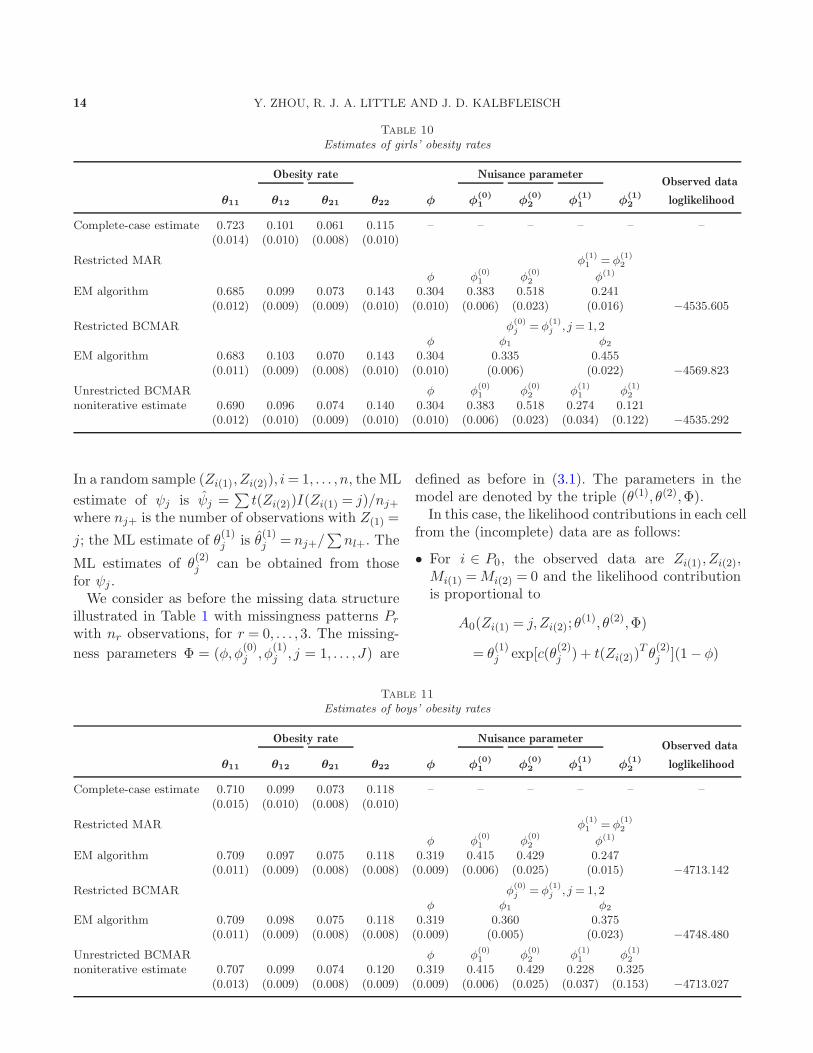
2. There is strong evidence thatthe restricted BCMAR model does not fit the data.On the other hand, lmax(M3) is close to lmax(M1),and we cannot differentiate the restricted MARmodelfrom the unrestricted BCMAR model.Similarly for the boys, the estimate from (3.8)

of {φ(1)1 , φ

(1)2 } in the unrestricted BCMAR model is

(0.228,0.325), which is in the parameter space, andclosed form estimates of the parameters are avail-able. Among 1000 bootstrap samples, only 28 sam-

ples yield the solutions of {φ(1)j } from (3.8) outside

BLOCK-CONDITIONAL MAR MODELS FOR MISSING DATA 13

Table 8

Estimates of parameters for data in Table 6B

Parameter of interest Nuisance parameter

θ11 θ12 θ21 θ22 θ31 θ32 φ φ(0)1 φ

(0)2 φ

(0)3 φ

(1)1 φ

(1)2 φ

(1)3

Unrestricted BCMARNoniterative estimate 0.103 0.309 0.188 0.188 0.069 0.144 0.198 0.130 0.286 0.168 multiple solutions in [0,1]3

EM algorithm 0.103 0.309 0.188 0.188 0.069 0.144 0.198 0.130 0.286 0.168 multiple solutions

Restricted BCMAR φ(0)j = φ

(1)j , j = 1,2,3

φ φ1 φ2 φ3

EM algorithm 0.100 0.307 0.189 0.193 0.067 0.144 0.198 0.154 0.328 0.197

Restricted MAR φ(1)1 = φ

(1)2 = φ

(1)3

φ φ(0)1 φ

(0)2 φ

(0)3 φ(1)

EM algorithm 0.101 0.311 0.184 0.190 0.068 0.146 0.198 0.130 0.286 0.168 0.362

Table 9

Tables of data from muscatine

coronary risk factor study

1981

1 2 Missing

Girls

1 701 98 4971977 2 59 111 183

Missing 408 139 174

Boys

1 699 98 5661977 2 72 116 141

Missing 473 125 196

Notes: 1 = not obese, 2 = obese.

of the parameter space. The likelihood ratio testyields strong evidence against the restricted BC-MAR model, with −2(lmax(M2) − lmax(M1)) =−2(−4748.48 + 4713.03) = 70.9 on two degrees offreedom. On the other hand, lmax(M3) is close tolmax(M1), and the restricted MAR model seems tobe satisfactory (Table 11).The models considered above show a small effect

on the fitted values of obesity rates and their stan-dard errors. For boys, the marginal distributions of1981 obesity rates are quite similar for those with1977 obesity rates observed or not. If we consideronly the cases with 1977 obesity rates observed, thenoniterative block-monotone reduced ML estimatesof obesity rates for the unrestricted BCMAR modelare ML estimates, and these are close to ML esti-mates in the restricted BCMAR and MAR models.Furthermore, φ̂

(0)1 and φ̂

(0)2 are close to one another,

which suggests a MCAR mechanism. As a conse-quence, complete-case estimates of obesity rates arealso similar to those in three models considered above.For girls, for the same reason, noniterative block-monotone reduced ML estimates of obesity rates forthe unrestricted BCMAR model are ML estimatesand are close to those in the restricted BCMAR andMAR models. However, φ̂

(0)1 and φ̂

(0)2 are quite dif-

ferent, and, as a consequence, complete-case esti-mates of obesity rates are not similar to those inthe other three models.

7. TWO BLOCK BCMAR DATA WITHOUTCOMES FROM THE EXPONENTIAL

FAMILY DISTRIBUTION

Suppose, as before, that Z(1) takes values 1, . . . , J

with probabilities θ(1)j where

∑

θ(1)j = 1. The model

in Section 3 is generalized here to allow Z(2) to havean exponential family distribution of full rank. Thus,we suppose that the density of Z(2) given Z(1) is

f(Z(2)|Z(1) = j, θ(2))

= a(Z(2)) exp[c(θ(2)j ) + t(Z(2))

T θ(2)j ],

where j = 1, . . . , J , θ(2)j and t(Z(2)) are vectors of

dimension V , and c is a real-valued function. Thisfamily includes the exponential and normal distri-bution (with variance known or unknown) as wellas the multivariate normal, normal linear regressionand generalized linear models with canonical links.The mean of t(Z(2)) given Z(1) = j is given by theV -dimensional vector

ψj = ψ(θ(2)j ) =

∂c(θ(2)j )

∂θ(2)j

.

14 Y. ZHOU, R. J. A. LITTLE AND J. D. KALBFLEISCH

Table 10

Estimates of girls’ obesity rates

Obesity rate Nuisance parameterObserved data

θ11 θ12 θ21 θ22 φ φ(0)1 φ

(0)2 φ

(1)1 φ

(1)2 loglikelihood

Complete-case estimate 0.723 0.101 0.061 0.115 – – – – – –(0.014) (0.010) (0.008) (0.010)

Restricted MAR φ(1)1 = φ

(1)2

φ φ(0)1 φ

(0)2 φ(1)

EM algorithm 0.685 0.099 0.073 0.143 0.304 0.383 0.518 0.241(0.012) (0.009) (0.009) (0.010) (0.010) (0.006) (0.023) (0.016) −4535.605

Restricted BCMAR φ(0)j = φ

(1)j , j = 1,2

φ φ1 φ2

EM algorithm 0.683 0.103 0.070 0.143 0.304 0.335 0.455(0.011) (0.009) (0.008) (0.010) (0.010) (0.006) (0.022) −4569.823

Unrestricted BCMAR φ φ(0)1 φ

(0)2 φ

(1)1 φ

(1)2

noniterative estimate 0.690 0.096 0.074 0.140 0.304 0.383 0.518 0.274 0.121(0.012) (0.010) (0.009) (0.010) (0.010) (0.006) (0.023) (0.034) (0.122) −4535.292

In a random sample (Zi(1),Zi(2)), i= 1, . . . , n, the ML

estimate of ψj is ψ̂j =∑

t(Zi(2))I(Zi(1) = j)/nj+where nj+ is the number of observations with Z(1) =

j; the ML estimate of θ(1)j is θ̂

(1)j = nj+/

∑

nl+. The

ML estimates of θ(2)j can be obtained from those

for ψj .We consider as before the missing data structure

illustrated in Table 1 with missingness patterns Pr

with nr observations, for r = 0, . . . ,3. The missing-

ness parameters Φ = (φ,φ(0)j , φ

(1)j , j = 1, . . . , J) are

defined as before in (3.1). The parameters in themodel are denoted by the triple (θ(1), θ(2),Φ).In this case, the likelihood contributions in each cell

from the (incomplete) data are as follows:

• For i ∈ P0, the observed data are Zi(1),Zi(2),Mi(1) =Mi(2) = 0 and the likelihood contributionis proportional to

A0(Zi(1) = j,Zi(2); θ(1), θ(2),Φ)

= θ(1)j exp[c(θ

(2)j ) + t(Zi(2))

T θ(2)j ](1− φ)

Table 11

Estimates of boys’ obesity rates

Obesity rate Nuisance parameterObserved data

θ11 θ12 θ21 θ22 φ φ(0)1 φ

(0)2 φ

(1)1 φ

(1)2 loglikelihood

Complete-case estimate 0.710 0.099 0.073 0.118 – – – – – –(0.015) (0.010) (0.008) (0.010)

Restricted MAR φ(1)1 = φ

(1)2

φ φ(0)1 φ

(0)2 φ(1)

EM algorithm 0.709 0.097 0.075 0.118 0.319 0.415 0.429 0.247(0.011) (0.009) (0.008) (0.008) (0.009) (0.006) (0.025) (0.015) −4713.142

Restricted BCMAR φ(0)j = φ

(1)j , j = 1,2

φ φ1 φ2

EM algorithm 0.709 0.098 0.075 0.118 0.319 0.360 0.375(0.011) (0.009) (0.008) (0.008) (0.009) (0.005) (0.023) −4748.480

Unrestricted BCMAR φ φ(0)1 φ

(0)2 φ

(1)1 φ

(1)2

noniterative estimate 0.707 0.099 0.074 0.120 0.319 0.415 0.429 0.228 0.325(0.013) (0.009) (0.008) (0.009) (0.009) (0.006) (0.025) (0.037) (0.153) −4713.027

BLOCK-CONDITIONAL MAR MODELS FOR MISSING DATA 15

· (1− φ(0)j ).

• For i ∈ P1, the observed data are Zi(1),Mi(1) =0,Mi(2) = 1, and the likelihood contribution is pro-portional to

A1(Zi(1) = j; θ(1), θ(2),Φ)

= θ(1)j (1− φ)φ

(0)j .

• For i ∈ P2, the observed data are Zi(2),Mi(1) =1,Mi(2) = 0 and the likelihood contribution is pro-portional to

A2(Z(2); θ(1), θ(2),Φ)

= φ

J∑

j=1

θ(1)j exp[c(θ

(2)j ) + t(Z(2))

T θ(2)j ]

· (1− φ(1)j ).

• For i ∈ P3, no elements of Z(1) or Z(2) are observedand the data comprise Mi(1) = 1,Mi(2) = 1. Thelikelihood contribution is proportional to

A3(θ(1), θ(2),Φ) = φ

J∑

j=1

θ(1)j φ

(1)j .

The full observed-data likelihood is then theproduct of such terms and can be written as L =L0L1L2L3, where

L0 = (1− φ)n0

J∏

j=1

{(θ(1)j )n(0),j+(1− φ

(0)j )n(0),j+

· exp[c(θ(2)j ) + T T

0jθ(2)j ]},

L1 = (1− φ)n1

J∏

j=1

{(θ(1)j )n(1),j+(φ

(0)j )n(1),j+},

L2 = φn2∏

i∈P2

{

J∑

j=1

θ(1)j (1− φ

(1)j )

· exp[c(θ(2)j ) + t(Zi(2))

T θ(2)j ]

}

,

L3 = φn3

{

J∑

j=1

θ(1)j φ

(1)j

}n3

,

and T0j =∑

i∈P0t(Zi(2))I(Zi(1) = j).

An EM algorithm can readily be applied to max-imize the observed-data likelihood. At the E step,the underlying complete data in patterns P2 and

P3 can be replaced with their conditional expec-tations, whereas blocks P0 and P1 can be treatedas complete data. Alternatively, all four patternscan be incorporated into the EM approach, withthe complete data viewed as all the observationsZi(1),Zi(2), i= 1, . . . , n. For the data in block i ∈ P2,for example, the expectation step involves calculat-ing

E[I(Zi(1) = j)|Zi(2),Mi(1) = 1,Mi(2) = 0]

=θ(1)j (1− φ

(1)j ) exp[c(θ

(2)j ) + t(Zi(2))

T θ(2)j ]

∑Jl=1 θ

(1)l (1− φ

(1)l ) exp[c(θ

(2)l ) + t(Zi(2))

T θ(2)l ]

.

After missing data in each pattern are filled in fromthe E step, the M step computes the simple esti-mates given above for complete data.As in the multinomial case, the block-monotone

reduced ML estimates of the parameters θ(1)j , θ

(2)j ,

j = 1, . . . , J , are computed from patterns P0, P1, drop-ping the data from the other patterns. The corre-sponding block-monotone reduced likelihood of θ(1),θ(2) is

Lbm(P0, P1)∝L0 ×L1,

where the factors in the parameters Φ can be ignoredin L0,L1. Unlike the multinomial case, these block-monotone reduced ML estimates are typically notfull ML estimates, since there is information about

the parameters θ(2)j in the excluded patterns.

8. DISCUSSION

Most of the work on MNAR mechanisms concernsselection or pattern-mixture models, and extensionsto include latent random effects that are applicableto repeated-measures data (Little, 1995). In this ar-ticle we consider block-sequential missing data mod-els, where the variables in the data set are dividedinto subsets, and the joint distribution of these vari-ables and their missing data indicators are factoredas a sequence. A characteristic of this class is thatdistributions of variables and their missing data in-dicators are interleaved, and combinations of selec-tion and pattern-mixture models can be developedwithin each block. Except for the work of Robins(1997), there appears to be very little existing liter-ature on missing data mechanisms of this type.Here we consider a class of block-sequential miss-

ing data which we call block-conditional MAR mod-els, in which missingness in successive blocks is al-lowed to depend on observed variables in the block

16 Y. ZHOU, R. J. A. LITTLE AND J. D. KALBFLEISCH

and both observed and unobserved data in earlierblocks. The proposed class is related to the modelswith 2 blocks described in Little and Zhang (2011),in the context of regression with missing data. Ablock-monotone reduced likelihood approach to esti-mating these models is described that yields consis-tent asymptotically normal estimates without spec-ifying the distribution of the missing-data mecha-nism. We examined here the BCMAR model in somedetail for the case of bivariate categorical data, andshowed that maximization of the block-monotonereduced likelihood can yield fully efficient ML esti-mates, when associated estimates of parameters ofthe missing-data mechanism lie inside the parame-ter space. We also discussed more briefly the casewhere the variable in the second block comes froman exponential family, and inference based on theblock-monotone reduced likelihood approach is notin general fully efficient. In future work we plan tostudy other BCMAR models involving more thantwo blocks, continuous and categorical variables andmissing data within each block, and fully observedcovariate information.The BCMAR model discussed here is related to

the “latent ignorable” missing data mechanisms pro-posed to model missing data in the presence of non-compliance with a treatment (Frangakis and Rubin,1999; Peng, Little and Raghunathan, 2004). In thesecases, there is a binary compliance variable that in-dicates whether an individual would comply with atreatment if assigned to it. In a clinical trial, this in-dicator is fully observed for individuals in the activetreatment group, but is completely missing for indi-viduals in the control group, since they do not haveaccess to the active treatment. The latent ignorablemodel assumes MAR within subpopulations definedby the compliance indicator. Our BCMAR model,applied to that setting, generalizes this structure byallowing missing data for the stratifying variable.The BCMAR model (1.5) is just one of many pos-

sible block-sequential missing-data models, obtainedby placing restrictions on the parameters of the dis-tributions in each block. Future work might considerproperties of models obtained by imposing other pa-rameter restrictions, based on plausible assumptionsabout the nature of the missing data.

ACKNOWLEDGMENTS

We appreciate the constructive comments of tworeferees and an associate editor which greatly im-proved the paper.

REFERENCES

Baker, S. G. (1995). Marginal regression for repeated binary

data with outcome subject to non-ignorable nonresponse.Biometrics 51 1042–1052.

Baker, S. and Laird, N. (1985). Categorical response sub-ject to nonresponse. Technical Report, Dept. Biostatistics,

Harvard School of Public Health, Boston, MA.Birmingham, J. and Fitzmaurice, G. M. (2002). A

pattern-mixture model for longitudinal binary responseswith nonignorable nonresponse. Biometrics 58 989–996.

MR1945028Bishop, Y. M. M., Fienberg, S. E. and Holland, P. W.

(1975). Discrete Multivariate Analysis: Theory and Prac-

tice. MIT Press, Cambridge, MA. MR0381130Chen, T. and Fienberg, S. E. (1974). Two-dimensional con-

tingency tables with both completely and partially classi-fied data. Biometrics 30 629–642. MR0403086

Cox, D. R. (1975). Partial likelihood. Biometrika 62 269–276.MR0400509

Dempster, A. P., Laird, N. M. and Rubin, D. B. (1977).Maximum likelihood from incomplete data via the EM al-

gorithm (with discussion). J. Roy. Statist. Soc. Ser. B. 391–38. MR0501537

Ekholm, A. and Skinner, C. (1998). The muscatine chil-dren’s obesity data reanalysed using pattern mixture mod-

els. J. Roy. Statist. Soc. Ser. C. 47 251–263.Fay, R. E. (1986). Causal models for patterns of nonresponse.

J. Amer. Statist. Assoc. 81 354–365.

Frangakis, C. E. and Rubin, D. B. (1999). Addressingcomplications of intention-to-treat analysis in the com-bined presence of all-or-none treatment-noncompliance andsubsequent missing outcomes. Biometrika 86 365–379.

MR1705410Fuchs, C. (1982). Maximum likelihood estimation and model

selection in contingency tables with missing data. J. Amer.

Statist. Assoc. 77 270–278.

Hartley, H. O. (1958). Maximum likelihood estimation fromincomplete data. Biometrics 14 174–194.

Heckman, J. I. (1976). The common structure of statisticalmodels of truncation, sample selection and limited depen-

dent variables, and a simple estimator for such models.Ann. Econ. Soc. Meas. 5 475–492.

Lipsitz, S. R., Ibrahim, J. G. and Zhao, L. P. (1999).

A weighted estimating equation for missing covariate datawith properites similar to maximum likelihood. J. Amer.

Statist. Assoc. 94 1147–1160. MR1731479Lipsitz, S. R., Parzen, M. and Molenberghs, G. (1998).

Obtaining the maximum likelihood estimates in incompleteR×C contingency tables using a Poisson generalized linearmodel. J. Comput. Graph. Statist. 7 356–376.

Little, R. J. A. (1993). Pattern-mixture models for multi-

variate incomplete data. J. Amer. Statist. Assoc. 88 125–134.

Little, R. J. A. (1995). Modeling the drop-out mechanismin repeated-measures studies. J. Amer. Statist. Assoc. 90

1112–1121. MR1354029Little, R. J. A. and Rubin, D. B. (2002). Statistical Anal-

ysis with Missing Data. Wiley, Hoboken, NJ. MR1925014

BLOCK-CONDITIONAL MAR MODELS FOR MISSING DATA 17

Little, R. J. A. and Zhang, N. (2011). Subsample ignorable

likelihood for regression analysis with missing data. J. Roy.

Statist. Soc. Ser. C 60. To appear.

Meng, X.-L. and Rubin, D. B. (1993). Maximum likelihood

estimation via the ECM algorithm: A general framework.

Biometrika 80 267–278. MR1243503

Peng, Y. H., Little, R. J. A. and Raghunathan, T. E.

(2004). An extended general location model for causal in-

ferences from data subject to noncompliance and missing

values. Biometrics 60 598–607. MR2089434

Robins, J. M. (1997). Non-response models for the analysis

of non-monotone non-ignorable missing data. Stat. Med. 16

21–37.

Robins, J. M. and Gill, R. (1997). Non-response models forthe analysis of non-monotone ignorable missing data. Stat.Med. 16 39–56.

Rubin, D. B. (1976). Inference and missing data (with dis-cussion). Biometrika 63 581–592. MR0455196

Rubin, D. B. (1987). Multiple Imputation for Nonresponse in

Surveys. Wiley, New York. MR0899519Rubin, D. B., Stern, H. and Vehovar, V. (1995). Handling

“don’t know” survey responses: The case of the Slovenianplebiscite. J. Amer. Statist. Assoc. 90 822–828.

Woolson, R. F. and Clarke, W. R. (1984). Analysis ofcategorical incomplete longitudinal data. J. Roy. Statist.

Soc. Ser. A 147 87–99.