Continuous-time model identification from sampled data: Implementation issues and performance...

Continuous-time model identification from sampled data: implementation issues and performance

evaluation

H. GARNIER{*, M. MENSLER{ and A. RICHARD{

This paper deals with equation error methods that fit continuous-time transfer function models to discrete-time datarecently included in the CONTSID (CONtinuous-Time System IDentification) Matlab toolbox. An overview of themethods is first given where implementation issues are highlighted. The performances of the methods are then evaluatedon simulated examples by Monte Carlo simulations. The experiments have been carried out to study the sensitivity ofeach approach to the design parameters, sampling period, signal-to-noise ratio, noise power spectral density and type ofinput signal. The effectiveness of the CONTSID toolbox techniques is also briefly compared with indirect methods inwhich discrete-time models are first estimated and then transformed into continuous-time models. The paper does notconsider iterative or recursive algorithms for continuous-time transfer function model identification.

1. Introduction

Identification of continuous-time (CT) linear time-

invariant (LTI) models for continuous-time dynamic

processes was the initial goal in the earliest works on

system identification. However, due to the success of

digital computers and the availability of digital data

acquisition boards, most system identification schemes

usually aim at identifying the parameters of discrete-

time (DT) models based on sampled input–output

data. Well-established theories are available (Ljung

1987, Soderstrom and Stoica 1989) and many applica-

tions have been reported. Over the last few years there

has been strong interest in continuous-time approaches

for system identification from sampled data (Soderstrom

et al. 1997, Unbehauen and Rao 1998, Johansson et al.

1999, Garnier et al. 2000, Pintelon et al. 2000, Bastogne

et al. 2001, Wang and Gawthrop 2001, Young 2002 a,

Young et al. 2003). Identification of CT models is in-

deed a problem of considerable importance in various

disciplines such as economics, control and signal

processing.

A simplistic way of estimating the parameters of a

CT model by an indirect approach is to use the sampled

data to first estimate a DT model and then convert it

into an equivalent CT model. However, the second step,

i.e. obtaining an equivalent CT model from the esti-

mated DT model, is not always easy. Difficulties are

encountered whenever the sampling time is either too

large or too small. Whereas a large sampling interval

may lead to loss of information, making it very small

may create numerical problems due to the fact that the

poles are constrained to lie in a very small area of the z-

plane close to the unit circle. Some conversion methods

use the matrix logarithm which may produce complex

arithmetic when the matrix has negative eigenvalues.

Moreover, the zeros of the DT model are not as easily

transformable to CT equivalents as the poles are.

An alternative approach is to directly identify a

continuous-time model from the discrete-time data.

Since the equation error (EE) is a linear algebraic func-

tion of the model parameters, EE model structure-

based methods have been widely followed for direct

continuous-time model identification from sampled

data. The basic problem of this EE approach is with

handling of the non-measurable time-derivatives and the

removal of asymptotic bias on the parameter estimates

when the noise is at a high level. In an EE context, CT

model identification indeed implies measurement or gen-

eration of the input–output time-derivatives. The need

to generate these time-derivatives may be eliminated by

applying ‘linear dynamic operations’ to the sampled

input–output data according to Unbehauen and Rao

(1987). These ‘linear dynamic operations’ can be inter-

preted as input and output signal pre-processing. Many

pre-processing approaches have been developed.

Surveys (Young 1981, Unbehauen and Rao 1990,

Sagara and Zhao 1991) and books (Unbehauen and

Rao 1987, Sinha and Rao 1991) offer a broad overview

of many of the available techniques. However, no com-

mon tool including the main CT parametric model iden-

tification approaches was available. The CONtinuous-

Time System IDentification (CONTSID) Matlab tool-

box has been developed to fill this gap (Garnier and

Mensler 2000). It is a collection of the main approaches

International Journal of Control ISSN 0020–7179 print/ISSN 1366–5820 online # 2003 Taylor & Francis Ltdhttp://www.tandf.co.uk/journals

DOI: 10.1080/0020717031000149636

INT. J. CONTROL, 2003, VOL. 76, NO. 13, 1337–1357

Received 24 January 2002. Revised 22 January 2003.Accepted 10 May 2003.

*Author for correspondence. e-mail: [email protected]

{Centre de Recherche en Automatique de Nancy(CRAN), CNRS UMR 7039, Universite Henri Poincare,Nancy 1, BP 239, F-54506 Vandœuvre-les-Nancy Cedex,France.

{Nissan Motor Co., Ltd. Nissan Research Center,Electronics and Information Technology ResearchLaboratory 1, Natsushima-cho, Yokosuka-shi, Kanagawa237-8523, Japan.

found in the literature and has been developed in a setup

similar to the System IDentification (SID) Matlab1

toolbox.

The goal of this paper is twofold. It first aims at

giving a unifying overview of EE methods for direct

CT model identification from sampled data included in

the CONTSID Matlab toolbox where implementation

issues are highlighted. The second objective is to evalu-

ate the performance of the implemented methods

through Monte Carlo simulations. The experiments

have been carried out to study the sensitivity of each

approach to the user parameters, sampling period,

signal-to-noise ratio, noise power spectral density and

type of input signal. Furthermore, the performance of

the direct CONTSID toolbox techniques has also been

compared with the indirect approach with the objec-

tive to illustrate some particular problems of the latter.

The paper is organized in the following way. Section

2 briefly defines the parameter estimation problem. Then

} 3 is devoted to the presentation of the general schemefor EE model structure-based estimation. An overview

of the three classes of pre-processing operations is given

in } 4. Section 5 provides the performance evaluationresults. Some discussions and conclusions are given in

} 6.It is important to note that the paper does not con-

sider recursive or iterative approaches to continuous-

time identification, although both are possible. In par-

ticular, it does not evaluate the recursive and iterative

simplified refined instrumental variable method for

continuous-time model identification (SRIVC: see

Young and Jakeman 1980). This approach involves a

method of adaptive prefiltering based on an optimal

statistical solution to the problem and is a logical exten-

sion of the more heuristically defined state-variable filter

(SVF) or generalized Poisson moment functionals

(GPMF) methods (see Young 2002 a, b). This optimal

technique presents the clear advantage of not requiring

manual specifications of prefilter parameters and pro-

viding the covariance matrix for the parameter esti-

mates. The SRIVC is available in the CAPTAIN

Matlab toolbox (the RIVC algorithm: see http://www.

es.lancs.ac.uk/cres/captain/) and has been implemented

recently in the CONTSID toolbox (Huselstein et al.

2002, Huselstein and Garnier 2002). However, it was

not available when the present comparative study was

carried out.

2. Problem formulation

Consider a single-input single-output continuous-

time linear time-invariant causal system that can be

described by

yuðtÞ ¼ GoðpÞuðtÞ ð1Þ

with

GoðpÞ ¼BoðpÞAoðpÞ

BoðpÞ ¼ bo0 þ bo1pþ � � � þ bompm

AoðpÞ ¼ ao0 þ ao1pþ � � � þ aonpn; aon ¼ 1; n � m

where uðtÞ is the input signal and yuðtÞ the systemresponse to uðtÞ, p is the differential operator, i.e.pxðtÞ ¼ dxðtÞ=dt.The polynomials AoðpÞ and BoðpÞ are assumed to be

relatively prime and all the roots of the polynomialAoðpÞ are assumed to have negative real parts; thesystem under study is therefore assumed to be asympto-tically stable.Equation (1) describes the output at all values of the

continuous-time variable t and can also be written as

ao0yuðtÞ þ ao1yð1Þu ðtÞ þ � � � þ yðnÞu ðtÞ

¼ bo0uðtÞ þ bo1uð1ÞðtÞ þ � � � þ bomu

ðmÞðtÞ;

subject to u0; y0u ð2Þ

where xðiÞðtÞ denotes the i th time-derivative of the con-tinuous-time signal xðtÞ.

GoðpÞ describes the true dynamics of the systemwhich is subject to an arbitrary set of initial conditions

u0 ¼ ½uð0Þ uð1Þð0Þ � � � uðm�1Þð0Þ ð3Þ

y0u ¼ ½yuð0Þ yð1Þu ð0Þ � � � yðn�1Þu ð0Þ ð4Þ

It is further assumed that the disturbances that can-not be explained from the input signal can be lumpedinto an additive term voðtÞ so that

yðtÞ ¼ GoðpÞuðtÞ þ voðtÞ ð5Þ

The disturbance term voðtÞ is assumed to be indepen-dent of the input uðtÞ, i.e. the case of the open-loopoperation of the system is considered. For the identifica-tion problem, it is also assumed that the continuous-time signals uðtÞ and yðtÞ are sampled at regular time-interval Ts.The objective is then to build a model of (5) based on

sampled input and output data. Models of the followingform are considered

yuðtkÞ ¼ Gðp; �ÞuðtkÞ

yðtkÞ ¼ yuðtkÞ þ vðtkÞ

)ð6Þ

1338 H. Garnier et al.

where xðtkÞ denotes the sample of the continuous-timesignal xðtÞ at time-instant t ¼ kTs and Gðp; �Þ is theplant model transfer function given by

Gðp; �Þ ¼ BðpÞAðpÞ ¼

b0 þ b1pþ � � � þ bmpm

a0 þ a1pþ � � � þ anpn ;

an ¼ 1; n � m; ð7Þand � ¼ ½an�1 � � � a0 bm � � � b0T.It is emphasized that direct methods presented in

this paper focus on identifying the parameters of theplant transfer function Gðp; �Þ rather than the additivenoise appearing in (5). The disturbance term is modelledhere as a zero-mean discrete-time noise sequencedenoted as vðtkÞ.Note that only a few methods focus on the contin-

uous-time noise modelling where voðtÞ is assumed tohave rational power spectral density

�voði!Þ ¼ �2jHoði!; �Þj ð8Þ

conveniently modelled as

vðtÞ ¼ Hðp; �ÞeðtÞ ð9Þwhere eðtÞ is a continuous-time white noise. Theseapproaches are indeed mainly developed in time-seriesanalysis, i.e. models with no input (uðtÞ � 0) (Tuan1997, Fan et al. 1999, Mossberg 2000, Pham 2000,Soderstrom and Mossberg 2000). Some extensionshave however been made to handle the case of contin-uous-time ARX models (Soderstrom et al. 1997).To avoid mathematical difficulties in considering

continuous-time stochastic processes (Astrom 1970),hybrid modelling approaches have been proposedwhere a continuous-time plant model with a discrete-time noise model is estimated (Young and Jakeman1980, Johansson 1994, Pintelon et al. 2000). Theapproach taken in this paper can therefore be consid-ered as a hybrid model structure estimation method. Thedifference lies in the fact that, even if a discrete-timenoise sequence is assumed to affect the output signal,no noise model will be identified.The identification problem can now be stated as

follows: assume the orders n and m as known, and esti-mate the parameter vector � of the continuous-timeplant model from N sampled measurements of theinput and the output ZN ¼ uðtkÞ; yðtkÞf gNk¼1.

3. General scheme for EE model structure-based

estimation

The general scheme for the EE model structure-based estimation of a continuous-time model from dis-crete-time measurements requires two stages

. the primary stage which consists in finding a pre-processing method to generate some measures ofthe process signals and their time-derivatives. This

stage also includes finding an approximating ordiscretizing technique so that the pre-processingoperation can be performed in a purely digitalway from sampled input–output data;

. the secondary or estimation stage in which the CTparameters are estimated within the framework ofa parameter estimation method.

Most of the well-known linear regression methodsdeveloped for DT parameter estimation can be extendedto the CT case with slight differences or modifications.Therefore the main departure from the DT model iden-tification is due to the primary stage.This primary stage arises out of the time-derivative

measurement problem. Indeed, in contrast with the dif-ference equation model, the differential equation modelis not a linear combination of samples of only themeasurable process input and output signals. It alsocontains derivative terms which are not available asmeasurement data in most practical cases. There areonly a few exceptions as in the case of mechanicalsystems, e.g. where time-derivatives such as velocityand acceleration can be directly measured.

3.1. The primary stage

Most of the various pre-processing operations maybe interpreted as a low-pass filtering of input and outputsignals (Sagara and Zhao 1991). For convenience ofpresentation, pre-processing operations will be pre-sented in the sense of this pre-filtering scheme.Let us first consider the differential equation model

given by (6) in the noise-free case

a0yuðtÞ þ a1yð1Þu ðtÞ þ � � � þ yðnÞu ðtÞ ¼ b0uðtÞ þ b1u

ð1ÞðtÞþ � � � þ bmu

ðmÞðtÞ; subject to u0; y0u ð10Þ

Applying the one-sided Laplace transform to bothsides of (10) yields

Xn�1i¼0

aisiYuðsÞ þ snYuðsÞ ¼

Xmi¼0

bisiUðsÞ þ

Xn�1i¼0

cisi ð11Þ

or

AðsÞYuðsÞ ¼ BðsÞUðsÞ þ CðsÞ ð12Þ

with

AðsÞ ¼Xn�1i¼0

aisi þ sn; BðsÞ ¼

Xmi¼0

bisi; CðsÞ ¼

Xn�1i¼0

cisi

ð13Þ

where s represents the Laplace variable while YuðsÞ andUðsÞ are respectively the Laplace transform of yuðtÞ and

Continuous-time model identification 1339

uðtÞ. The coefficients ci depend on the initial conditionsand are given by

ci ¼Xn�1j¼i

ajþ1yð j�iÞu ð0Þ �

Xm�1

j¼i

bjþ1uð j�iÞð0Þ;

for i ¼ 0; . . . ;m� 1 ð14Þ

ci ¼Xn�i

j¼i

ajþ1yð j�iÞu ð0Þ; for i ¼ m;mþ 1; . . . ; n ð15Þ

Assume now that a causal analogue pre-filter has aLaplace transform FðsÞ. Applying the filter to both sidesof (12) yields

AðsÞFðsÞYuðsÞ ¼ BðsÞFðsÞUðsÞ þ FðsÞCðsÞ ð16Þ

or

Xn�1i¼0

aiYiu; f ðsÞ þ Yn

u; f ðsÞ ¼Xmi¼0

bi Uif ðsÞ þ

Xn�1i¼0

ci �if ðsÞ

ð17Þ

where

Yiu; f ðsÞ ¼ siFðsÞYuðsÞ; Ui

f ðsÞ ¼ siFðsÞUðsÞ

�if ðsÞ ¼ siFðsÞ

)ð18Þ

Denoting the inverse Laplace transforms as

yðiÞu; f ðtÞ ¼ L�1½Yi

u; f ðsÞ; uðiÞf ðtÞ ¼ L�1½Ui

f ðsÞ

�ðiÞf ðtÞ ¼ L�1½�if ðsÞ

9=; ð19Þ

we have

Xn�1i¼0

aiyðiÞu; f ðtÞ þ y

ðnÞu; f ðtÞ ¼

Xmi¼0

bi uðiÞf ðtÞ þ

Xn�1i¼0

ci �ðiÞf ðtÞ ð20Þ

At the time-instant t ¼ tk, considering the additivenoise on the output measurement, equation (20) can berewritten as

Xn�1i¼0

aiyðiÞf ðtkÞ þ y

ðnÞf ðtkÞ ¼

Xmi¼0

bi uðiÞf ðtkÞ þ

Xn�1i¼0

ci �ðiÞf ðtkÞ

þ "EEðtk; �Þ ð21Þ

where "EEðtk; �Þ denotes the equation error also termedas ‘generalized equation error’ (Young 1981).Note that the whole set of filtered variables of the

process signals and also their time-derivatives appearingin (21) can be generated by two identical filters operatingon the process input and output. Since only the sampledversions of the continuous-time signals are available, thefiltered variables can only be computed from the digitalimplementation of FðsÞ which will generate someapproximations. By taking into account the digital

implementation of the analogue filter, equation (21)becomes

Xn�1i¼0

ai�yyðiÞf ðtkÞ þ �yy

ðnÞf ðtkÞ ¼

Xmi¼0

bi �uuðiÞf ðtkÞ þ

Xn�1i¼0

ci ��ðiÞf ðtkÞ

þ �""EEðtk; �Þ ð22Þ

where �xxðiÞf ðtkÞ represents the digital implementation of

the analogue filtering FðsÞ of xðiÞðtÞ at time-instantt ¼ tk. The equation error

�""EEðtk; �Þ ¼ "EE;�ðtkÞ þ ðtk; �Þ ð23Þ

where ðtk; �Þ denotes the error term introduced by thedigital implementation of the analogue filtering on theprocess signals.The noise-free case of continuous-time model identi-

fication is indeed not as straightforward as its discrete-time counterpart. The digital implementation error termðtk; �Þ can however be reduced by choosing a smallsampling interval Ts. Without loss of generality andfor notational simplicity, this latter noise will beneglected in the following. Note also in equation (21)the presence of additional terms which resulted fromthe process input–output initial conditions (see ‘imple-mentation issues’ in } 4).There is a range of choice for the pre-processing

required in the primary stage of an EE model struc-ture-based estimation scheme. Each method is charac-terized by specific advantages such as mathematicalconvenience, simplicity in numerical implementationand computation, physical insight, accuracy and others.However, all perform some pre-filtering on the processsignals. Process signal pre-filtering is indeed a very use-ful and important way to improve the statistical effi-ciency in system identification and yield lower varianceof the parameter estimates. An interesting discussion onthe relationship between pre-filtering, noise models andprediction for discrete-time models was given recently inLjung (1987). A similar analysis has been very recentlyproposed for the continuous-time model case in Wangand Gawthrop (2001). The pre-filter Fðs) plays the samerole as pre-filters in the case of discrete-time model iden-tification, in addition to its role in avoiding direct differ-entiation of noisy signals. For this purpose, the pre-filterFðsÞ should be designed in such a way that it has fre-quency response characteristics close to the system to beidentified, as first mentioned in Young (1976), andYoung and Jakeman (1979, 1980). The latter referencesdevelop optimal approaches to continuous-time TFmodel estimation, in which the prefilters are automati-cally selected in an iterative or recursive/iterative man-ner (see comments in } 1). In the present, non-iterativecontext, the prefilter parameters should, as far as poss-ible, be chosen with these requirements in mind.


3.2. The secondary stage

For simplicity, it is assumed in this part that thedifferential equation model (10) is initially at rest.Note however that in the general case the initial con-dition terms do not vanish in (21). Whether they requireestimation or they can be neglected depends upon theselected pre-processing method. This will be discussedunder ‘implementation issues’ in } 4.In the case of EE model structure-based estimation,

the model can be estimated by the following fit

��N ¼ argmin�

VNð�;ZNÞ ð24Þ

VNð�;ZNÞ ¼XNk¼1

"2EEðtk; �Þ ð25Þ

To estimate the parameters ai; bi, equation (21) canbe reformulated using the transformed variables intostandard linear regression form as

yðnÞf ðtkÞ ¼ �Tf ðtkÞ�þ "EEðtk; �Þ ð26Þ

with

�Tf ðtkÞ

¼ �yðn�1Þf ðtkÞ � � � � yf ðtkÞ u

ðmÞf ðtkÞ � � � uf ðtkÞ

h ið27Þ

� ¼ ½an�1 � � � a0 bm � � � b0T ð28Þ

From N available samples of the input and outputsignals, the least-squares (LS) estimate that minimizesthe sum of the squared errors is given by

��LSN ¼XNi¼1

�f ðtkÞ�Tf ðtkÞ" #�1XN

i¼1�f ðtkÞy

ðnÞf ðtkÞ ð29Þ

provided the inverse exists.It is however well known that the conventional least-

squares method delivers biased estimates in the presenceof general cases of measurement noise. One of the sim-plest solutions to the asymptotic bias problem associ-ated with the basic LS algorithm is to use instrumentalvariable (IV) methods since they do not require a prioriknowledge of the noise statistics. A bootstrap estimationof IV type where the instrumental variable is built froman auxiliary model is considered here (Young 1970). Theinstrument is given by

��Tf ðtkÞ

¼ �yyðn�1Þu; f ðtkÞ � � � �yyu; f ðtkÞ u

ðmÞf ðtkÞ � � � uf ðtkÞ

h ið30Þ

where

yyu; f ðtkÞ ¼ FðpÞyyuðtkÞsubject to zero initial conditions ð31Þ

and yyuðtkÞ is the noise-free output calculated from

yyuðtkÞ ¼ Gðp; ��LSN ÞuðtkÞ ð32Þ

The IV-based estimated parameters are then givenby

��IVN ¼XNi¼1

��f ðtkÞ�Tf ðtkÞ" #�1XN

i¼1��f ðtkÞy

ðnÞf ðtkÞ ð33Þ

provided that the inverse exists.This bootstrap estimation of IV type has been

selected since it does not require a noise model estima-tion and can be used with any of the considered pre-processing methods. Note that the IV estimate canalso be calculated in a recursive or recursive/iterativemanner (Young 1970, Young and Jakeman 1980).

4. Review of the pre-processing operations

Pre-processing operations are traditionally dividedinto the following three main classes of methods:

. linear filters;

. integral methods;

. modulating functions.

In order to illustrate the principle of the pre-pro-cessing operations belonging to the three classes avail-able in the CONTSID toolbox, the noise-free differentialequation model (10) is considered.

4.1. Linear filter methods

4.1.1. Main idea. This case corresponds exactly towhat has been presented in } 3.1. In that case, the pre-processing operation takes the form of a linear filterFðsÞ of general form given by

FðsÞ ¼Pmf

i¼0 bfi s

iPnfi¼0 a

fi s

i; a f

n ¼ 1; nf � mf ð34Þ

The filter should be stable and its order nf should begreater or equal to the order n of the process model. Thechoice of the filter can be made from a frequencyresponse point of view. Basically as previously men-tioned, the bandwidth of the filter should approximatelyencompass the frequency band covered by the process tobe identified in order to keep on the one hand all rele-vant information, and remove high frequency noise onthe other (Young 1970, 1976, Young and Jakeman 1980,Isermann et al. 1992).


4.1.2. State-variable filter (SVF) approach. The diffi-culty in choosing a priori a filter is that it leads to afilter of the form of a cascade of identical or non-iden-tical first order filters. This method was proposed byYoung (1964) and was referred to as the method ofmultiple filters. In the case of identical first orderfilters, the minimal-order state-variable filter has theform

F1ðsÞ ¼

sþ �

� �n

ð35Þ

where n is the system order. This minimal-order SVFform presents the advantage of having a unique free-parameter � to be a priori chosen by the user (sincemost of the time ¼ � is set). It has therefore beenselected for implementation in the CONTSID toolboxas the basic SVF method.

4.1.3. Generalized Poisson Moment Functionals(GPMF) approach. Another method which is closelyrelated to the SVF method but suggested much later isthe generalized Poisson moment functionals (GPMF)approach (Saha and Rao 1983, Unbehauen and Rao1987). The minimal-order GPMF method may indeedbe considered as a particular case of the SVFapproach where the filter has the form

F2ðsÞ ¼

sþ �

� �nþ1ð36Þ

Note therefore for the comparative study that willfollow (and therefore in the CONTSID toolbox), thatthe SVF and GPMF approaches mainly differ only fromthe order of the filter considered. Recent GPMF devel-opments were proposed in Garnier et al. (1994, 1997,2000) and Bastogne et al. (2001).

4.1.4. Implementation issues.

. Initial conditions. The SVF and GPMFapproaches make it possible to estimate the initialcondition terms along with the model parameters(Young 1964, Saha and Rao 1983). However,treating them as an additional set of unknownsfirst complicates the parameter estimation. Fromequation (21), it may be noted that although theinitial condition terms do not vanish, they decayexponentially provided the system is stable andbecome insignificant quite quickly. Thus, if theSVF or GPMF algorithms are taken for a largeobservation time T , the terms related to the initialconditions may be neglected after a timeT0 ¼ k0Ts. The estimation algorithm is thenapplied over ½T0;T , where T0 has to be chosencomparable to the settling time of the filter. Thenumber of parameters to be estimated can in thisway be reduced substantially and this is surely

advantageous with regard to computation effortsand numerical properties.

. Digital implementation of the SVF and GPMF fil-ters. The analogue SVF or GPMF-based filtershave to be implemented in digital form in orderto make it convenient for computers to handle it.This problem is well known but should be treatedin a proper way since miscalculations generated bythe digital implementation can have severe influ-ence on the quality of the estimated model. Usingan appropriate control canonical form (Isermannet al. 1992), the state-space representations of thecontinuous-time SVF or GPMF-based filter haveto be either integrated by the Runge–Kuttamethod or discretized by using an appropriatemethod.

. SVF and GPMF filter design parameters . As theorder in the case of minimal SVF and GPMFapproaches is respectively fixed to n and nþ 1,the design parameter to be specified by the useris the cut-off frequency of both filters only. Thiscut-off frequency should be chosen in order toemphasize the frequency band of interest and itis advised in general to choose it a little bit largerthan the frequency bandwidth !c of the system tobe identified.

4.2. Integral methods

4.2.1. Main idea. The main idea of these methods isto avoid the differentiation of the data by performingan order n integration. These integral methods can beroughly divided into two groups. The first group is ofnumerical integration methods and orthogonal func-tion methods, performs a basic integration of the dataand particularly attention has to be paid to the initialcondition issue. The integration is performed for thesemethods over a stretched window. The second familyof methods is of the linear integral filter (LIF) and thereinitialized partial moments (RPM) approaches, per-forms advanced integrations which have the propertyof making the initial conditions vanish. This propertycomes from the fact that the integration window is amoving integration window for the LIF method, and atime-shifting window for the RPM method.

4.2.2. Integral method over a stretched window. Inte-grating n-times equation (10) leads to the followingintegral equation

Xn�1i¼0

aiy½n�iðtÞ þ yðtÞ ¼

Xmi¼0

biu½n�iðtÞ þ

Xn�1i¼0

citi

i!ð37Þ


where

x½iðtÞ¼4ðt0

ð�10

� � �ð�i�20

xð�i�3Þ d�i�3 � � � d�1 ð38Þ

The termPn�1

i¼0 ciðti=i!Þ represents the effects of input–

output initial conditions.From a filtering point of view, the integral methods

may be interpreted as a pre-filtering operation where

F3ðsÞ ¼1

snð39Þ

Integrals appearing in (37) can be numerically computedeither by numerical integration techniques such as thetrapezoidal approximation (TPF) or the Simpson’s rule(Dai and Sinha 1991) or by decomposing the signalsover a set of r orthogonal functions LðtÞ (Unbehauenand Rao 1987, Mohan and Datta 1991). The orthogonalfunction methods implemented in the CONTSID tool-box are based on Walsh and block-pulse functions(BPF) in the case of PCBF, and on the first and secondkinds of Chebychev polynomials (CHEBY1 andCHEBY2), Hermite (HERMIT), Laguerre (LAGUER)and Legendre polynomials (LEGEND) for the orthogo-nal polynomials, and the Fourier trigonometric func-tions (FOURIE).

Implementation issues:

. Initial conditions. This is a crucial issue of thisfamily of methods, since initial condition termsnot only fail to vanish in (37), but also increasewith time. They are therefore to be included in theparameter vector in order to take their influenceinto account. The number of parameters to beestimated is in this way inflated and this is surelynot advantageous in regards to computation effortand numerical properties.

. Digital implementation. This is another drawbackof these methods since integration has to be per-formed over the entire span of the observationtime. Obviously, for a very large number of dataand/or for a large number of orthogonal functionsof the basis LðtÞ, the calculation might not be pos-sible due to the memory limitation of the compu-ter.

. Design parameters. One of the nice features ofnumerical integration techniques is that they donot require any design parameters to be a priorispecified by the user. In the case of orthogonalfunctions, the design parameter is the number ofterms r considered in the truncated expansion oforthogonal series. The a priori choice of r is atricky problem. At first, indeed, r must be chosenas high as possible to get appropriate informationabout the input–output of the process band-

width. However r must also be limited becauseof the decomposition of high frequency noiseand the numerical error due to the approximationof the repeated integrations. The following heur-istic thumb rule may help

r � q� np q 2 ½5; 20 ð40Þ

with np ¼ nþmþ 1.

4.2.3. Integral method over a moving window (LIF).The main idea of the linear integral filter (LIF)method lies in the calculations of the n successive time-integrals of the input-output signals. However, unlikethe previously presented integral methods, the integra-tions are performed over a moving window of lengthlTs (Sagara and Zhao 1990). Equation (37) thenbecomes

Xn�1i¼0

aiInfyðiÞðtÞg þ InfyðnÞðtÞg ¼Xmi¼0

biInfuðiÞðtÞg ð41Þ

with

InfxðtÞg¼4ðtt�lTs

ð�1�1�lTs

. . .

ð�n�1�n�1�lTs

xð�nÞ d�n � � � d�1

ð42Þ

From a filtering point of view, the LIF method maybe interpreted as a a pre-filtering operation where

F4ðsÞ ¼1� e�lTss

s

!n

ð43Þ


. Initial conditions. The time-integrals are evaluatedover a moving window of length lTs. This propertypresents the advantage over the stretched windowintegral methods to make the initial conditionsdisappear (Sagara and Zhao 1990).

. Digital implementation. Although the LIF methodhas a linear filtering form, the time-integrationform of the LIF is preferred for the implementa-tion. Since the input–output data are sampled,the discretized nth time-integrals of the i th time-derivatives of the signal xðkÞ can be approachedsuch as (Sagara and Zhao 1990)

Iifxð jÞðkÞg � J jxðkÞ ð44Þ

with

J j ¼ ð1� q�lÞ j ð f0 þ f1q�1 þ � � � þ flq

�lÞn�j ð45Þ

The coefficients of the polynomial J j given at (45),depend on the numerical integration method used


such as the trapezoidal or a Simpson’s rule of inte-gration.

. Design parameter. The design parameter of themethod is the coefficient l of the time-integrationwindow length. It can be selected by using the LIFgain expression given by

jF4ð j!Þj ¼��lTs

sinð !=!sÞ !=!s

��n

¼��lTs sincð!=!sÞ

��n

with !s ¼2

lTs

ð46Þ

so as to make the system and the filter cut-offfrequencies coincide. Note that the LIF filtergain depends on the sampling interval used, thedesign parameter will therefore depend on thesampling time used.

4.2.4. Time-weighing integral method over a time-shift-ing window (RPM). The main idea of this methodintroduced by Trigeassou (1987) is to perform a time-weighing of the input–output signals and a time-shift-ing before integrating them. In such a case, equation(2) becomes

�yun ðtÞ �

Xn�1i¼0

an�i �yui ðtÞ ¼

Xmi¼0

bm�i�ui ðtÞ ð47Þ

with

�yui ðtÞ ¼ �

ð tt0

pið�Þ yuðt� ttþ �Þ d� 0 � i < n

�ui ðtÞ ¼

ð tt0

pið�Þ uðt� ttþ �Þ d� 0 � i < n

9>>>>=>>>>;

ð48Þ

The functions pið�Þ are time-weighing functions andare given by (Jemni and Trigeassou 1996)

p0ð�Þ ¼�nðtt� �Þn�1

ðn� 1Þ! ttn ; � � � ; pið�Þ ¼ ð�1Þi dip0ð�Þd� i

ð49Þ

The integration window is ½0; tt. This approach hasbeen named the reinitialized partial moment (RPM)method. As the LIF method, the RPM method can beexpressed from a filtering point of view since the methodhas made a time-convolution appear between the weigh-ing functions pið�Þ and the input–output signals. Theassociated filter f5ðtÞ is an infinite impulse response filter,the expression of which is

f5ðtÞ ¼ðtt� tÞn tn�1

ðn� 1Þ! ttn t 2 ½0; tt ð50Þ

The terms of (48) can be rewritten as

�yui ðtÞ ¼ � d

if5ðtÞdti

? yuðtÞ 0 � i < n

�ui ðtÞ ¼

dif5ðtÞdti

? uðtÞ 0 � i < n

9>>>=>>>;

ð51Þ

However, on account of a discontinuity of the filterf5ðtÞ at t ¼ 0, the terms �yu

n ðtÞ and �unðtÞ are

�yun ðtÞ ¼ yuðtÞ �

ð tt0

pnð�Þ yuðt� ttþ �Þ d�

�unðtÞ ¼ uðtÞ þ

ð tt0

pnð�Þ uðt� ttþ �Þ d�

9>>>>=>>>>;

ð52Þ

Note that it has been chosen here to classify theRPM approach in the integral method family becauseof the integration performed on the differential equationmodel. This latter could also be considered as a linearfilter approach.


. Initial conditions. Although the RPM method islinked to the integral methods, it is in fact animproved version: it operates a reinitialization ofthe data and this results in the elimination of theinitial conditions from (47). This is one of theadvantages of the present method.

. Digital implementation. As the LIF method, anumerical integration using the integral form ofthe RPM method is preferred for the implementa-tion. The expressions of the modified terms in (48)and (52) are used for the parameter estimationrather than the terms of (51). Simpson’s rule ofintegration or a piece-wise constant rule is useddepending on the assumptions made on theinput–output signals.

. Design parameter. The design parameter is kk withtt ¼ kkTs. Experience shows that the RPM methodis not too sensitive to the user parameter. Thechoice of the design parameter is then very simple.This constitutes a very attractive feature of theRPM method because the design parameter choicestage can be the most insidious among thedifferent steps of the continuous-time modelidentification methods. Note however that forimplementation reasons, kk has to be even.

4.3. Modulating function approach

4.3.1. Main idea. The general formulation of the mod-ulating function approach was first developed by Shin-brot in order to estimate the parameters of linear andnon-linear systems (Shinbrot 1957). Further develop-


ments have been carried out and spawned several ver-sions based on different modulating functions. Theyinclude the Fourier based functions either under a tri-gonometric form or under a complex exponentialform; Spline-type functions; Hermite functions; and,more recently, the Hartley-based functions. A veryimportant advantage of using Fourier- and Hartley-based modulating functions is that the system identifi-cation can be equivalently posed entirely in the fre-quency domain which makes it possible to use efficientDFT/FFT techniques. These two methods are there-fore well suited for digital implementation and havebeen included in the CONTSID toolbox.A function ’�;nðtÞ is a modulating function of order

n relative to a fixed time interval ½0;T , where � is anindex, if it is sufficiently smooth and possesses the fol-lowing property for l 2 ½0; n� 1

dl’�;nðtÞdtl

��t¼0

¼dl’�;nðtÞdtl

��t¼T

¼ 0 ð53Þ

The modulating function and its first ðn� 1Þ derivativestherefore vanish at both end points of the observationtime interval. The idea is to multiply both sides of (10)by such a set of modulating functions and integrate byparts over ½0;T with the latter property (53). This leadsto the relation

Xn�1i¼0

ð�1Þi aiðT0

yuðtÞ’ðiÞ�;nðtÞ dtþ ð�1Þn

ðT0

yuðtÞ’ðnÞ�;nðtÞ dt

¼Xmi¼0

ð�1ÞibiðT0

uðtÞ’ðiÞ�;nðtÞ dt ð54Þ

The prime reasons for using such modulating func-tions are first to circumvent the need to reconstruct thepossibly noisy and unknown input and output deriva-tives by transferring them into derivatives of chosenfunction ’�;nðtÞ; and secondly, to avoid estimatingunknown initial conditions.By denoting

�yun�ið�!0Þ ¼ ð�1Þið2 =!o

0

yuðtÞ’ðiÞ�;nðtÞ dt ð55Þ

�un�ið�!0Þ ¼ ð�1Þið2 =!o

0

uðtÞ’ðiÞ�;nðtÞ dt ð56Þ

where � ¼ 0; . . . ;M (M � nþmþ 1) is called the mod-ulating frequency index; M is the design parameter ofthe method; !0 ¼ 2 =T is the resolving frequency; n isthe model order; T is the observation time interval.Equation (54) can then be written into standard regres-sion form as in (26).

4.3.2. Fourier modulating functions (FMF). Based onShinbrot’s method of moment functionals, Pearson

suggested first to use the Fourier modulating functions(FMF) defined by (Pearson et al. 1994)

’�;nðtÞ ¼1

Te�i�!0tðe�i!0t � 1Þn

¼ 1

T

Xnk¼0

ð�1Þn�kn

k

!e�iðkþ�Þ!0t ð57Þ

wherenk

� �denotes the binomial coefficient defined as

n

k

� �¼ n!

k! ðn� kÞ!

4.3.3. Hartley modulating functions (HMF). Thismodulating function relies on the casðtÞ functiondefined by

casðtÞ¼4 cosðtÞ þ sinðtÞ ð58Þ

The Hartley modulating function is then defined by(Unbehauen and Rao 1998)

�;nðtÞ ¼Xnk¼0

ð�1Þkn

k

� �cas ðnþ �� kÞ!0tð Þ ð59Þ

Although the Hartley modulating function is closelyrelated to the Fourier modulating function, the HMFmethod is real-valued. This is presented as an advantagesince the input–output signals are real-valued (Bracewell1986). Moreover the Hartley spectra can be computedefficiently with the help of discrete Hartley transforms.


. Initial conditions. A clear advantage of the modu-lating function methods is that because of prop-erty (53), the effects of initial conditions disappear.

. Digital implementation. As mentioned previously,another interesting advantage of using Fourier-and Hartley-based modulating functions is thatthe system identification can be equivalentlyposed entirely in the frequency domain and theFourier and Hartley functionals can be computedby efficient DFT/FFT techniques.

. FMF and HMF design parameters. The designparameter to be specified by the user is index M.This latter should be chosen so that M!0 is closeto the bandwidth !c of the system to be identifiedin order to keep all relevant information about thesystem.

Note that in the case of FMF and HMF methods,the pre-filtering operation is performed in the frequencydomain. Therefore, no filter form can be explicitly given,in contrast with the case of integral and linear filtermethods presented above.


4.4. Pre-processing operations implemented in theCONTSID toolbox

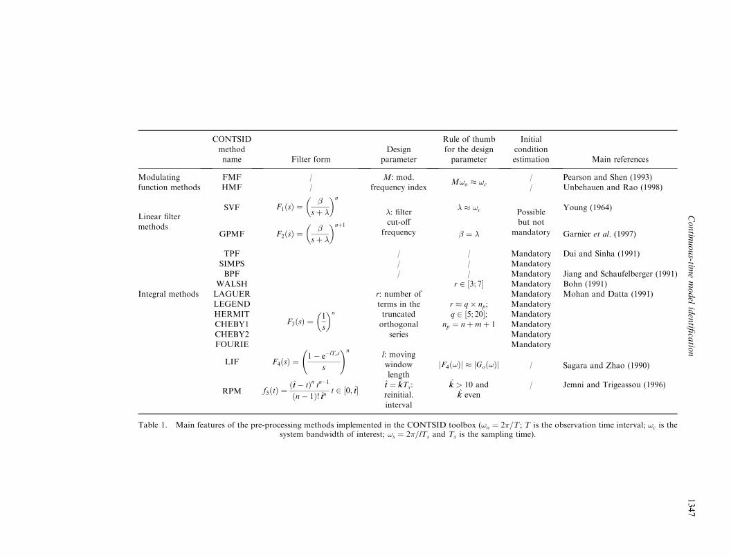
Table 1 summarizes for each pre-processing methodincluded in the CONTSID toolbox its main featuresalong with rule of thumb for choosing the user par-ameter. This makes a total of 16 pre-processing methodsimplemented in the CONTSID toolbox. All availableapproaches have been associated with LS and IV algor-ithms (see } 3).The following comments can be made from table 1.

If the initial conditions explicitly disappear when themethods like FMF, HMF, LIF and RPM are used,they remain in the input–output equation for all therest of the methods. While it is possible to neglecttheir effects after a certain time in the case of linear filtermethods, taking them into account is required for allintegral methods over a stretched window. This, ofcourse, presents a major drawback of increasing thenumber of parameters to be estimated. Rules of thumbfor choosing the design parameters of each approach arealso given. All design parameters should be chosenaccording to the system bandwidth of interest. The latterhas therefore to be approximately known before handand this can be seen as a difficulty. However, the valuesof most design parameters can be iteratively updatedeither manually or automatically by optimizing a costfunction related to the model fit to the data.Furthermore, as illustrated later, the methods whichperform well, are not too sensitive to their design par-ameters.There are several other approaches that cannot be

classified directly into any of the main three groups. Afirst interesting approach closely related to the linearfilter methods (SVF and GPMF) was proposed byJohansson (1994) and Chou et al. (1999) where an alge-braic reformulation of transfer function model is used.A second approach has also attracted a lot of attentionin the last few years which is based on replacing thedifferentiation operator with finite differences(Soderstrom et al. 1997).

5. Numerical examples

In this section, the performance of all the directmethods for CT model identification implemented inthe CONTSID toolbox was evaluated by Monte Carlosimulations. The approaches are first evaluated with thehelp of a second-order system. The effects of the pre-filter characteristics are particularly discussed. Thisallows us to select six methods which perform best.Then another comparative study on a more complexfourth-order process is presented. Here, the objective isto illustrate the effectiveness of the selected directmethods in various simulation conditions and to com-

pare them briefly to the indirect approach via discrete-time model estimation.Note that these comparative results do not include

evaluation of the SRIVC method mentioned in theintroduction section, since this was not part of theCONTSID toolbox at the time the present study wascarried out. However, the SRIVC method performs aswell as, and often better, than the other methods (Young2002 a, b, Huselstein et al. 2002).

5.1. Second-order system simulation study

5.1.1. Simulation conditions. The system considered inthis section is a linear second-order system with com-plex poles described by (Sagara and Zhao 1990)

GoðpÞ ¼K

ðp2=!2nÞ þ ð2�p=!nÞ þ 1ð60Þ

with K ¼ 1:25, !n ¼ 2 rad/s and � ¼ 0:7.The process considered here is a rather simple one.

However, it is sufficient to illustrate the main conclu-sions for this first comparative study. Note also thatsimilar results have been obtained in the case of previouscomparative studies performed on higher-order simu-lated systems (Mensler et al. 1999) and on real-lifedata (Mensler et al. 2000).The input signal is chosen as the following sum of

three sinusoidal signals (Sagara and Zhao 1990)

uðtÞ ¼ sinð0:714tÞ þ sinð1:428tÞ þ sinð2:142tÞ ð61ÞThe data generating system is given by the relations

yuðtkÞ ¼ GoðpÞuðtkÞ; subject to zero initial conditions

ð62Þ

yðtkÞ ¼ yuðtkÞ þ vðtkÞ ð63Þ

where fvðtkÞgNk¼1 is a zero-mean independent identicallydistributed (i.i.d.) gaussian sequence.For the computation of the noise-free output, analy-

tical expressions are used in order to avoid errors due tonumerical simulations. The sampling period is equal toTs ¼ 0:05 s while the number of samples is set to 1000.Monte Carlo simulations of 100 realizations are used fora signal-to-noise ratio (SNR) of 10 dB. The SNR isdefined as

SNR ¼ 10 logPyu

Pv

ð64Þ

where Pv represents the average power of the zero-meanadditive noise on the system output (e.g. the variance)while Pyu denotes the average power of the noise-freeoutput fluctuations.

5.1.2. Criteria. The criteria selected for the perfor-mance evaluation are the mean average square error(MSE) of the output and the empirical standard devia-


Contin

uous-tim

emodel

identifi

catio

n1347

CONTSID

method

name Filter form

Design

parameter

Rule of thumb

for the design

parameter

Initial

condition

estimation Main references

Modulating

function methods

FMF

HMF

/

/

M: mod.

frequency indexM!o � !c

/

/

Pearson and Shen (1993)

Unbehauen and Rao (1998)

Linear filter

methods

SVF

GPMF

F1ðsÞ ¼

sþ �

� �n

F2ðsÞ ¼

sþ �

� �nþ1

�: filtercut-off

frequency

� � !c

¼ �

Possible

but not

mandatory

Young (1964)

Garnier et al. (1997)

TPF / / Mandatory Dai and Sinha (1991)

SIMPS / / Mandatory

BPF / / Mandatory Jiang and Schaufelberger (1991)

WALSH r 2 ½3; 7 Mandatory Bohn (1991)

Integral methods LAGUER

F3ðsÞ ¼1

s

� �n

r: number of Mandatory Mohan and Datta (1991)

LEGEND terms in the r � q� np; Mandatory

HERMIT truncated q 2 ½5; 20; Mandatory

CHEBY1 orthogonal np ¼ nþmþ 1 Mandatory

CHEBY2 series Mandatory

FOURIE Mandatory

LIF F4ðsÞ ¼1� e�lTss

s

!nl: moving

window

length

jF4ð!Þj � jGoð!Þj / Sagara and Zhao (1990)

RPM f5ðtÞ ¼ðtt� tÞn tn�1

ðn� 1Þ! ttn t 2 ½0; tt tt ¼ kkTs:

reinitial.

interval

kk > 10 andkk even

/ Jemni and Trigeassou (1996)

Table 1. Main features of the pre-processing methods implemented in the CONTSID toolbox (!o ¼ 2 =T ; T is the observation time interval; !c is thesystem bandwidth of interest; !s ¼ 2 =lTs and Ts is the sampling time).

tion (�SE) of the average square error (SE) of the out-put defined by

MSE ¼ 1

Nexp

XNexpi¼1

SEðiÞ ð65Þ

�2SE ¼ 1

Nexp

XNexpi¼1

ðSEðiÞ �MSEÞ2 ð66Þ

where

SE ¼ 1

N

XNk¼1

"2ðtkÞ ð67Þ

"ðtkÞ ¼ yuðtkÞ � yyuðtkÞ ¼ yuðtkÞ � Gðp; ��NÞuðtkÞ ð68Þ

where yu and yyu represent the noise-free output of thesystem and the simulated output of the estimated modelrespectively; Nexp is the number of Monte Carlo simula-tion experiments. Simulation results with these latterperformance indices are representative of the generalresults obtained and will be therefore presented here.A last performance index will also be considered. Itrepresents the ‘stability rate’ of the methods, that is,the number of stable models estimated during theMonte Carlo simulations. Note that unstable estimatedmodels are not used to compute the above performanceindices.

5.1.3. Effects of the design parameters. To study thesensitivity of the pre-processing methods to their userparameters, Monte Carlo simulations were used. Thepre-processing operations were coupled with a IV algo-rithm built from an auxiliary model (see } 3.2).For methods where it is advised to choose the user

parameters so that the frequency response of the filterencompasses the process bandwidth (FMF, HMF, SVF,GPMF, LIF), the user parameter was varied in the inter-val ½!n=10; 10!n (where !n is the natural frequency ofthe process to be identified). In the case of orthogonalfunction methods, the design parameter was variedaccording to the heuristic rule given in table 1.From the numerous simulations done, it turned out

that the behaviour of the methods is different: the effi-ciency of most of integral methods over a stretchedwindow is really deteriorated (stability rate < 100%,MSE > 10�2) while methods based on modulating func-tions (FMF and HMF), linear filters (SVF and GPMF)and the two particular integral methods (LIF and RPM)present, in the considered range of their user parameters,very good performance (stability rate ¼ 100%,MSE < 10�2). The design of the filters is not criticalwhen these six methods are associated with the IV tech-nique.

Note that acceptable estimation results wereobtained with integral methods in a previous compara-tive study of CT model identification methods for asecond-order simulation example in the case of lownoise level on the output signals (Homssi and Titli1991). However, it seems that in the case of mediumto low SNR, integral methods should be avoided.The poor performance of integral methods over a

stretched window can also be partly explained by con-sidering the design parameter r of the orthogonal func-tion methods; in other words, the number of functionsin the orthogonal basis. If the number of functions in thebasis is too small to allow a good reconstruction of theinput–output signals, the parametric estimation maythen be bad. But if r is high, the orthogonal functionmethods tend to reconstruct not only the output signal,but also the noise corrupting the signal: the quality ofthe estimated model is then poor. Even if the proposedrule of thumb may provide some help in choosing thedesign parameter, it remains difficult to choose a valuefor r that allows a good estimation of the parametersand circumvents the problem in case of noisy outputsignals.

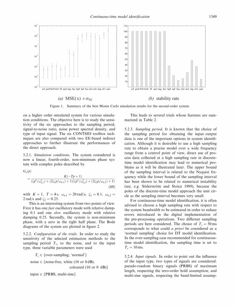
5.1.4. Parameter estimates when the design parametersare ‘optimally’ chosen. From the previous analysis, thevalue of the user parameters which minimized MSEfor each technique was selected. Then a Monte Carlosimulation of 100 realizations was performed with thesame level and type of additive noise. The results aredisplayed in figure 1 and illustrate the conclusionsdrawn in the previous section.The smaller the MSE and the higher the stability

rate, the better the method. The efficiency of most ofintegral methods over a stretched window is really dete-riorated in the presence of noise. This is first observedfrom the stability rate displayed in figure 1(b) which issmaller than 100% except for the Laguerre and Hermitemethods. Not only do these methods often lead tounstable models, but also when the estimated model isstable, its behaviour is very different from the actualsystem (MSE > 10�2, see figure 1(a)). Note that thethree methods which do not have any design parameters(BPF, TPF and SIMPS) perform poorly in the presenceof noise.To conclude, methods that are able to provide good

results are those which are robust to their design par-ameters; that is pre-processing techniques based onmodulating functions (FMF and HMF); on linear filters(SVF and GPMF); and on the two particular integralapproaches (LIF and RPM).

5.2. Fourth-order system simulation study

The performance of the six selected continuous-timemodel identification techniques was further investigated


on a higher order simulated system for various simula-tion conditions. The objective here is to study the sensi-tivity of the six approaches to the sampling period,signal-to-noise ratio, noise power spectral density, andtype of input signal. The six CONTSID toolbox tech-niques are also compared with two EE-based indirectapproaches to further illustrate the performances ofthe direct approach.

5.2.1. Simulation conditions. The system considered isnow a linear, fourth-order, non-minimum phase sys-tem with complex poles described by

GoðpÞ

¼ Kð�Tpþ 1Þððp2=!2n;1Þ þ ð2�1p=!n;1Þ þ 1Þððp2=!2n;2Þ þ ð2�2p=!n;2Þ þ 1Þ

ð69Þ

with K ¼ 1, T ¼ 4 s, !n;1 ¼ 20 rad/s, �1 ¼ 0:1, !n;2 ¼2 rad/s and �2 ¼ 0:25.This is an interesting system from two points of view.

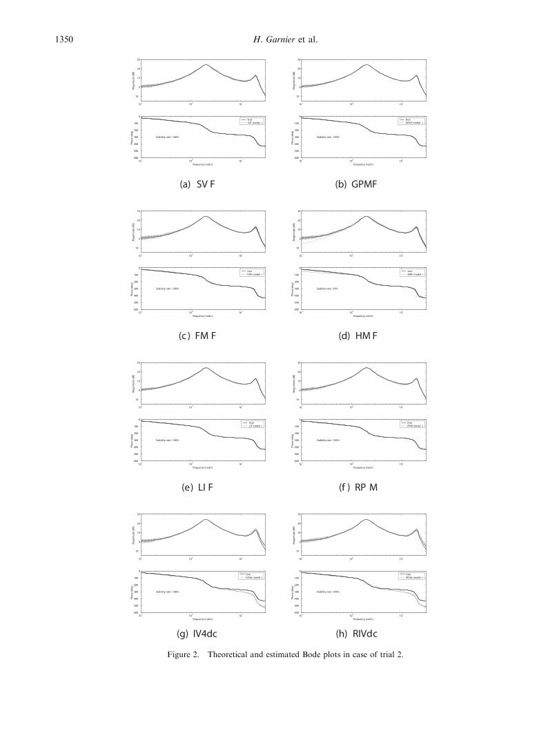
First it has one fast oscillatory mode with relative damp-ing 0:1 and one slow oscillatory mode with relativedamping 0:25. Secondly, the system is non-minimumphase, with a zero in the right half plane. The Bodediagrams of the system are plotted in figure 2.

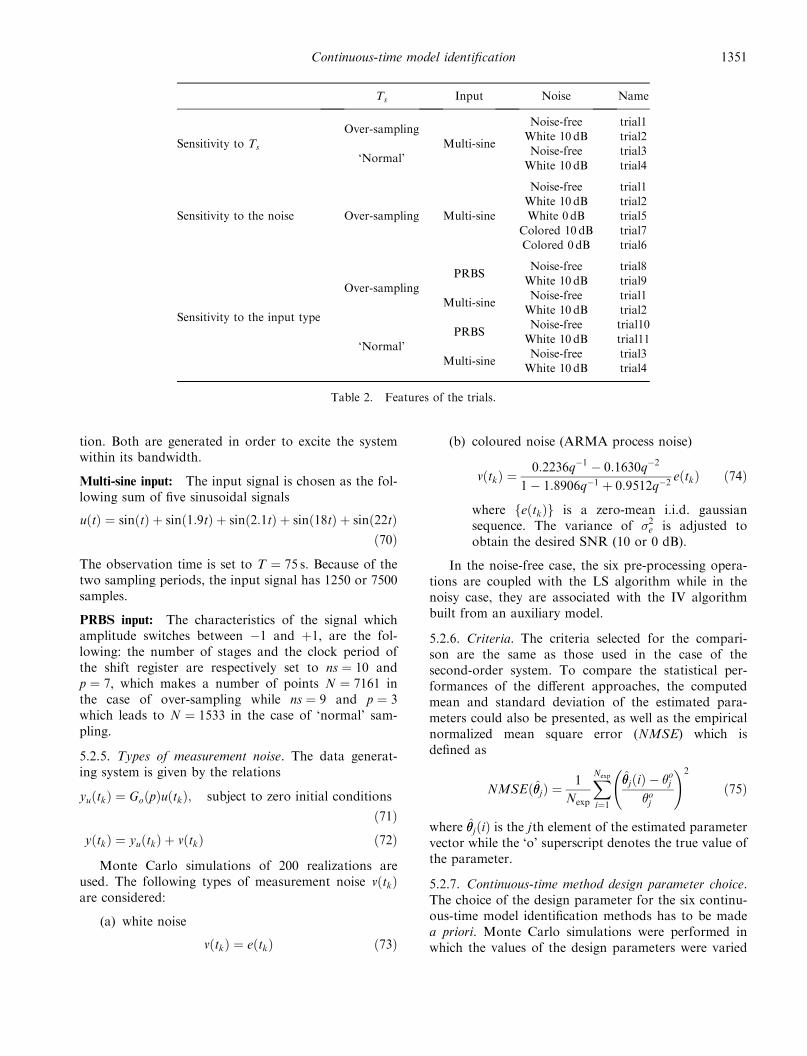
5.2.2. Configuration of the trials. In order to study thesensitivity of the selected estimation methods to thesampling period Ts, to the noise, and to the inputtype, three variable parameters were used

Ts 2 fover-sampling, ‘normal’g

noise 2 fnoise-free, white (10 or 0 dB);coloured (10 or 0 dB)g

input 2 fPRBS, multi-sineg

This leads to several trials whose features are sum-

marized in Table 2.

5.2.3. Sampling period. It is known that the choice of

the sampling period for obtaining the input–output

data is one of the important options in system identifi-

cation. Although it is desirable to use a high sampling

rate to obtain a precise model over a wide frequency

range from a control point of view, direct use of pro-

cess data collected at a high sampling rate in discrete-

time model identification may lead to numerical pro-

blems as it will be illustrated later. The upper bound

of the sampling interval is related to the Nyquist fre-

quency while the lower bound of the sampling interval

has been shown to be related to numerical instability

(see, e.g. Soderstrom and Stoica 1989), because the

poles of the discrete-time model approach the unit cir-

cle as the sampling interval becomes very small.

For continuous-time model identification, it is often

advised to choose a high sampling rate with respect to

the system bandwidth to be estimated in order to reduce

errors introduced in the digital implementation of

the pre-processing operations. Two different sampling

periods are here considered. The choice of Ts ¼ 50mscorresponds to what could a priori be considered as a

‘normal sampling’ choice for DT model identification.

In the over-sampling case recommended for continuous-

time model identification, the sampling time is set to

Ts ¼ 10ms.

5.2.4. Input signals. In order to point out the influence

of the input type, two types of signals are considered:

pseudo-random binary signals (PRBS) of maximum

length, respecting the zero-order hold assumption; and

multi-sine signals, respecting the band-limited assump-


svf pmf fmf hmf lif rpm lag her bpf tpf fou ch2 sim leg ch1 wal10

5

104

103

102

101

100

101

(a) MSE(x) ± SE

svf pmf fmf hmf lif rpm lag her bpf tpf fou ch2 sim leg ch1 wal

10

20

30

40

50

60

70

80

90

100

110

(b) stability rateσ

Figure 1. Summary of the best Monte Carlo simulation results for the second-order system.


101

100

101

10

0

10

20

30

Mag

nitu

de (d

B)

101

100

101

600

500

400

300

200

100

0

Stability rate : 100%

frequency (rad/s)

Phas

e (d

eg)

trueSVF model s

(a) SV F

101

100

101

10

0

10

20

30

Mag

nitu

de (d

B)

101

100

101

600

500

400

300

200

100

0


frequency (rad/s)

Phas

e (d

eg)

trueGPMF model s

(b) GPMF

101

100

101

10

0

10

20

30

Mag

nitu

de (d

B)

101

100

101

600

500

400

300

200

100

0


frequency (rad/s)

Phas

e (d

eg)

trueFMF model s

(c ) FM F

101

100

101

10

0

10

20

30

Mag

nitu

de (d

B)

101

100

101

600

500

400

300

200

100

0


frequency (rad/s)

Phas

e (d

eg)

trueHMF model s

(d) HM F

101

100

101

10

0

10

20

30

Mag

nitu

de (d

B)

101

100

101

600

500

400

300

200

100

0


frequency (rad/s)

Phas

e (d

eg)

trueLIF model s

(e) LI F

101

100

101

10

0

10

20

30

Mag

nitu

de (d

B)

101

100

101

600

500

400

300

200

100

0


frequency (rad/s)

Phas

e (d

eg)

trueRPM model s

(f ) RP M

101

100

101

10

0

10

20

30

Mag

nitu

de (d

B)

101

100

101

600

500

400

300

200

100

0


frequency (rad/s)

Phas

e (d

eg)

trueIV4dc model s

(g) IV4dc

101

100

101

10

0

10

20

30

Mag

nitu

de (d

B)

101

100

101

600

500

400

300

200

100

0


frequency (rad/s)

Phas

e (d

eg)

trueRIVdc model s

(h) RIVdc

Figure 2. Theoretical and estimated Bode plots in case of trial 2.

tion. Both are generated in order to excite the systemwithin its bandwidth.

Multi-sine input: The input signal is chosen as the fol-lowing sum of five sinusoidal signals

uðtÞ ¼ sinðtÞ þ sinð1:9tÞ þ sinð2:1tÞ þ sinð18tÞ þ sinð22tÞð70Þ

The observation time is set to T ¼ 75 s. Because of thetwo sampling periods, the input signal has 1250 or 7500samples.

PRBS input: The characteristics of the signal whichamplitude switches between �1 and þ1, are the fol-lowing: the number of stages and the clock period ofthe shift register are respectively set to ns ¼ 10 andp ¼ 7, which makes a number of points N ¼ 7161 inthe case of over-sampling while ns ¼ 9 and p ¼ 3which leads to N ¼ 1533 in the case of ‘normal’ sam-pling.

5.2.5. Types of measurement noise. The data generat-ing system is given by the relations

yuðtkÞ ¼ GoðpÞuðtkÞ; subject to zero initial conditions

ð71Þ

yðtkÞ ¼ yuðtkÞ þ vðtkÞ ð72Þ

Monte Carlo simulations of 200 realizations areused. The following types of measurement noise vðtkÞare considered:

(a) white noise

vðtkÞ ¼ eðtkÞ ð73Þ

(b) coloured noise (ARMA process noise)

vðtkÞ ¼0:2236q�1 � 0:1630q�2

1� 1:8906q�1 þ 0:9512q�2eðtkÞ ð74Þ

where feðtkÞg is a zero-mean i.i.d. gaussiansequence. The variance of �2e is adjusted toobtain the desired SNR (10 or 0 dB).

In the noise-free case, the six pre-processing opera-tions are coupled with the LS algorithm while in thenoisy case, they are associated with the IV algorithmbuilt from an auxiliary model.

5.2.6. Criteria. The criteria selected for the compari-son are the same as those used in the case of thesecond-order system. To compare the statistical per-formances of the different approaches, the computedmean and standard deviation of the estimated para-meters could also be presented, as well as the empiricalnormalized mean square error (NMSE) which isdefined as

NMSEð��jÞ ¼1

Nexp

XNexpi¼1

��jðiÞ � �oj�oj

!2ð75Þ

where ��jðiÞ is the jth element of the estimated parametervector while the ‘o’ superscript denotes the true value ofthe parameter.

5.2.7. Continuous-time method design parameter choice.The choice of the design parameter for the six continu-ous-time model identification methods has to be madea priori. Monte Carlo simulations were performed inwhich the values of the design parameters were varied


Ts Input Noise Name

Over-samplingNoise-free trial1

Sensitivity to TsWhite 10 dB trial2

‘Normal’

Multi-sineNoise-free trial3

White 10 dB trial4

Noise-free trial1

White 10 dB trial2

Sensitivity to the noise Over-sampling Multi-sine White 0 dB trial5

Colored 10 dB trial7

Colored 0 dB trial6

PRBSNoise-free trial8

Over-samplingWhite 10 dB trial9


Sensitivity to the input typeWhite 10 dB trial2

PRBSNoise-free trial10

‘Normal’White 10 dB trial11


White 10 dB trial4

Table 2. Features of the trials.

in the case of trial2 and trial4 simulation conditions.The value which minimized MSE of each techniquewas retained. For the minimal-order SVF and GPMFapproaches, the design parameter has been chosen to12:5 rad/s (with ¼ �). The design parameter of theFourier and Hartley modulating function methods hasbeen set to M!o ¼ 18 rad/s. The user parameters ofthe LIF and RPM methods, which depend upon thesampling interval of the data, have been chosen respec-tively as l ¼ 18 and kk ¼ 60 when Ts ¼ 10ms, and l ¼ 4and kk ¼ 24 when Ts ¼ 50ms.

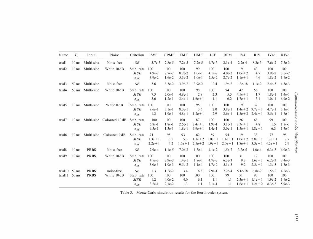
5.2.8. Monte Carlo simulation results. Monte Carlosimulation results are presented in table 3.

Sensitivity to the sampling period: Results given intable 3 for trial2 and trial9 can be compared withthose obtained in the case of trial4 and trial11 to studythe sensitivity of the selected continuous-time modelidentification techniques to the sampling time. The bestperformance of CT model identification methods is ex-pected in the case of oversampling. From these results,it appears that even if the performance deteriorates alittle for some methods (SVF, FMF, HMF, RPM), thesix CT approaches still deliver good results (stabilityrate ¼ 100%, MSE very small) for both cases of sam-pling period.

Sensitivity to the input type: Results given in table 3for trial2, trial4, trial9 and trial11 can be the basis forthe sensitivity study of the methods to the input type.It may be concluded that the six CT methods are nottoo sensitive to the type of input. The robustness tothe input type can be explained by the capacity of thesix CT methods to take the input nature into accountin the numerical implementation of the pre-processingoperations. All CT approaches are, therefore, able tocorrectly estimate the model parameters from excita-tion signals respecting the ZOH or the band-limitedassumptions, even if the GPMF and LIF present thebest performance here.

Sensitivity to the noise: The results obtained for thetwo types of noise (white or coloured) and the twoSNR are also given in table 3. In the case of whitenoise (trial4 and trial5), all CT methods are still effi-cient for the high level of noise (SNR=0dB). The re-sults in the case of coloured noise (trial6 and trial7)are less favourable for most CT methods when theSNR=0dB except the GPMF approach which is stillable to deliver good parameter estimates with almost100% of stable estimated models. Note that the IV-based HMF technique is the one which is the leastrobust to the noise level and type.

Direct versus indirect CT model identification approaches:

It is beyond the scope of this paper to compare direct

and indirect approaches to determine the parameters of

a continuous-time model. Each approach has its merits

and demerits. Some important problems and their sol-

utions appearing in the case of the indirect approach are

however illustrated. A more complete comparative

study of direct and indirect approaches can be found

in Zhao and Sagara (1994) and Rao and Garnier (2002).

Two IV-type DT model identification methods are

considered in the indirect approach where a DT model is

first identified and then converted in a CT model. The

two methods are the approximately optimal instrumen-

tal variable technique (four-step IV4 routine) Ljung

(1987) available in the Matlab1 System Identification

toolbox and the refined instrumental variable technique

(RIV routine) (Young and Jakeman 1979) available in

the CAPTAIN toolbox.{ These two IV-type methodshave been chosen because they are widely available

equation error type methods and the purpose is to com-

pare the EE methods discussed in the paper with other

EE methods.

The results obtained by the two DT estimation

methods on the original data set are also presented in

table 3 (see results for IV4 and RIV). The study of the

stability rate for the different techniques points out to

the clear difference between direct and indirect methods

in the case of both sampling strategies, even if the results

deteriorate a little bit less when the sampling interval is

equal to Ts ¼ 50ms which could as previously men-tioned have been considered as a ‘normal’ sampling

choice for DT model identification. Not only do the

DT methods more often lead to unstable models, but

also the behaviour of estimated stable models is signifi-

cantly different from that of the actual system (MSE is

higher). These results confirm the fact that while CT

model identification methods are very efficient here,

indirect methods using DT model identification tech-

niques may encounter problems due to numerical ill-

conditioning effects in the case of rapidly sampled

data. Note that in the case of the DT model identifica-

tion methods, SE has been computed from the estimated

DT model and not from the CT model converted from

the estimated DT model. This has been chosen to show

that the poor results obtained do not come from the

transformation step from the z-domain to the s-domain.

Note also that similar results have been obtained with

other widely available DT model identification tech-


{The authors are most grateful to Professor P. C. Youngfor proving the RIV routine and for his advice on the use ofthe algorithm. The original RIV algorithm was called refinedIV approximate maximum likelihood (RIVAML) (see Young1976) since it utilized the AML algorithm for ARMA noisemodel estimation. The simplified version of the RIV algorithmis used here which does not estimate a noise model.

Contin

uous-tim

emodel

identifi

catio

n1353

Name Ts Input Noise Criterion SVF GPMF FMF HMF LIF RPM IV4 RIV IV4d RIVd

trial1 10ms Multi-sine Noise-free SE 3.7e-3 7.8e-5 7.2e-5 7.2e-5 4.7e-3 2.1e-4 2.2e-4 8.3e-3 7.6e-2 7.3e-3

trial2 10ms Multi-sine White 10 dB Stab. rate 100 100 100 99 100 100 9 43 100 100

MSE 4.9e-2 2.7e-2 8.2e-2 1.0e-1 4.1e-2 4.0e-2 1.0e+2 4.7 3.9e-2 3.6e-2

�SE 3.9e-2 1.6e-2 5.3e-2 1.0e-1 2.5e-2 2.7e-2 1.1e+1 4.6 1.8e-2 1.5e-2

trial3 50ms Multi-sine Noise-free SE 3.6 3.3e-2 3.9e-2 3.9e-2 2.4 1.9e-2 1.3e-18 1.1e-2 2.4e-3 4.5e-3


MSE 7.3 2.0e-1 4.8e-1 2.8 2.3 5.5 4.5e+1 1.7 1.8e-1 1.4e-1

�SE 3.6 1.2e-1 3.4e-1 1.6e+1 1.1 6.2 1.7e+1 3.1 1.0e-1 6.9e-2


MSE 9.6e-1 3.1e-1 8.3e-1 3.6 2.0 3.8e-1 1.4e+2 9.7e+1 4.7e-1 3.1e-1

�SE 1.2 1.9e-1 4.8e-1 1.2e+1 2.9 2.6e-1 1.5e+2 2.4e+1 3.5e-1 1.5e-1

trial7 10ms Multi-sine Coloured 10 dB Stab. rate 100 100 100 87 100 100 26 68 99 100

MSE 6.8e-1 1.8e-1 2.5e-1 2.4e+1 1.9e-1 3.1e-1 8.3e+1 4.8 1.5 1.8e-1

�SE 9.3e-1 1.3e-1 1.8e-1 6.9e+1 1.4e-1 3.0e-1 1.5e+1 1.8e+1 6.3 1.3e-1

trial6 10ms Multi-sine Coloured 0 dB Stab. rate 74 95 93 62 89 94 19 33 77 95

MSE 1.3e+1 3.5 5.3 1.3e+2 1.0e+1 1.1e+1 1.0e+2 2.8e+1 1.7e+1 2.7

�SE 2.2e+1 4.2 1.5e+1 2.5e+2 1.9e+1 2.0e+1 1.8e+1 3.3e+1 4.2e+1 2.9

trial8 10ms PRBS Noise-free SE 7.9e-4 1.1e-5 7.0e-2 1.3e-1 4.1e-2 1.5e-7 3.3e-5 1.0e-4 6.3e-3 6.0e-3

trial9 10ms PRBS White 10 dB Stab. rate 100 100 100 100 100 100 31 12 100 100

MSE 4.5e-3 2.9e-3 1.4e-1 1.8e-1 4.7e-2 6.3e-3 9.3 1.6e+1 6.2e-3 7.4e-3

�SE 3.0e-3 1.9e-3 9.5e-2 1.1e-1 1.7e-2 5.1e-3 9.2 2.5e+1 1.3e-3 1.3e-3

trial10 50ms PRBS noise-free SE 1.3 1.2e-2 3.4 6.3 9.9e-1 7.2e-4 5.1e-18 6.8e-2 1.5e-2 4.6e-3

trial11 50ms PRBS White 10 dB Stab. rate 100 100 100 100 100 99 51 90 100 100

MSE 1.2 4.0e-2 4.0 6.1 1.1 1.1 2.3e+1 1.1e+1 1.9e-2 1.6e-2

�SE 3.2e-1 2.1e-2 1.3 1.1 2.1e-1 1.1 1.6e+1 1.2e+2 8.3e-3 5.9e-3

Table 3. Monte Carlo simulation results for the fourth-order system.

niques such as OE, PEM and N4SID routines (Rao and

Garnier 2002).

It is common practice to treat rapidly sampled data

in DT model identification by low-pass digital filtering

and decimating the original data record. The results

obtained by the two indirect approaches when the orig-

inal data sets have been pre-filtered and resampled at

Ts ¼ 100ms, are also presented in table 3 (see resultsfor IV4d and RIVd where ‘d’ is used to denote the deci-

mated data case). The performance of the two indirect

methods is now very close to that of the direct tech-

niques. The results given in table 3 illustrate also the

overall superiority of the RIV over the IV4 method.

Table 4 can be used to compare the statistical perform-

ances in case of trial2. Note the presence of two addi-

tional estimated parameters for the numerator in the

case of the indirect approaches (see results for IV4dc

and RIVdc where ‘c’ is used to denote the CT model

converted from the estimated DT model). Bode dia-

grams for all estimated CT models in case of trial2 are

also plotted in figure 2. The estimated Bode plots by the

two indirect approaches, although quite close over the

main frequency range, are not as good as the estimated

Bode plots by the direct methods at frequencies above

!n;1=20 rad/s. These discrepancies come from the addi-

tional zeros along with from the DT to the CT-domain

conversion stage. Note that the phase Bode diagrams of

the DT models have much closer agreement than the

converted CT models. A better answer can probably

be obtained by fitting to the Bode diagrams of the DT

models. This however seems hardly worthwhile since the

Bode plots are still not defined close to and above the

Nyquist frequency; and the direct CT model estimation

is much easier.

To sum up, it may be concluded from the extensive

Monte Carlo simulations performed on this more com-

plex fourth-order process that the overall performance

of six IV-based CT model identification techniques is

very good. It has been confirmed by the simulation

experiments that a relatively small sampling period is

not acceptable in the indirect approach. A solution

based on low-pass pre-filtering and decimation can


b3 b2 b1 b0 a3 a2 a1 a0

Method True value 0 0 �6400 1600 5 408 416 1600

SVF ��j �6359.7 1576.5 4.8 406.9 412.6 1596.0

��j 178.0 133.2 0.2 2.7 11.3 13.6

NMSEð��jÞ 8.1e-4 7.1e-3 2.9e-3 5.0e-5 8.0e-4 7.8e-5

GPMF ��j �6394.5 1596.1 5.0 408.5 415.6 1602.3

��j 111.9 101.0 0.2 2.4 7.2 11.4

NMSEð��jÞ 3.0e-4 3.9e-3 1.1e-3 3.6e-5 3.0e-4 5.2e-5

FMF ��j �6393.4 1601.0 5.0 408.3 415.8 1601.3

��j 202.7 167.4 0.3 5.8 13.2 27.2

NMSEð��jÞ 9.9e-4 1.1e-2 3.1e-3 2.0e-4 9.9e-4 2.9e-4

��j �6384.7 1581.2 5.0 408.2 415.3 1602.3

��j 250.0 198.0 0.3 6.2 15.1 30.8

NMSEð��jÞ 1.5e-3 1.5e-2 3.0e-3 2.3e-4 1.3e-3 3.7e-4

LIF ��j �6463.1 1608.3 5.0 411.0 420.0 1612.7

��j 150.7 111.3 0.2 2.6 9.3 13.4

NMSEð��jÞ 6.5e-4 4.8e-3 1.7e-3 9.4e-5 5.8e-4 1.3e-4

RPM ��j �6372.6 1603.2 5.0 408.3 414.4 1600.7

��j 169.6 118.0 0.2 2.5 10.6 13.5

NMSEð��jÞ 7.1e-4 5.4e-3 1.5e-3 3.7e-5 6.5e-4 7.1e-5

IV4dc ��j �7.0 336.9 �6603.7 1658.9 5.0 412.9 423.8 1620.6

��j 0.8 13.2 150.4 103.7 0.2 3.8 9.5 17.8

NMSEð��jÞ 1.6e-3 5.5e-3 9.9e-4 2.3e-4 8.6e-4 2.9e-4

RIVdc ��j �6.7 330.8 �6538.7 1703.1 5.0 411.3 419.7 1610.8

��j 0.7 12.5 113.6 97.8 0.2 3.5 7.1 15.7

NMSEð��jÞ 7.8e-4 7.9e-3 9.2e-4 1.4e-4 3.7e-4 1.4e-4

Table 4. Monte Carlo simulation results for the fourth-order system in case of trial2.

however be used to solve the numerical ill-conditioningproblems. The calculation of the continuous-time modelparameters from the identified discrete-time model isnevertheless not without difficulty.

6. Discussion and conclusion

In this paper, a unifying overview has been presentedof 16 pre-processing operations that have been used forequation error parameter estimation in direct continu-ous-time model identification from sampled data.Implementation issues for each approach have beenhighlighted and rules of thumb for choosing the designparameters have been proposed. These methods areavailable in the CONTSID Matlab toolbox which canbe freely downloaded at http://www.cran.uhp-nancy.fr/The CONTSID toolbox provides the possibility of

trying out and easily testing a large number of methodsavailable for the direct identification of continuous-timetransfer functions. The performances of the sixteenmethods considered in the paper have then beenthoroughly analysed by Monte Carlo simulation withthe objective of evaluating their sensitivity to designparameters, sampling period, signal-to-noise ratio,power spectral density of the noise, and type of inputsignal.From numerous simulation studies and also from

real-life data applications, integral methods over astretched window, which require the estimation of initialcondition terms and, therefore, lead to an augmentednumber of parameters to be estimated, perform poorlyin the presence of medium to high measurement noiselevel, apart from having a high sensitivity to their userparameters. However, six of the methods presented exhi-bit very good performances: these are based on linearfilters (GPMF and SVF), on modulating functions(FMF and HMF), and on the two particular types ofintegral methods (LIF and RPM). The final choice of aparticular approach will probably depend on the taste orexperience of the user since they have nearly the samequality of overall performance. It is, therefore, notnecessary to be able to tell which of the approaches is‘best’. Experience says that each may have its ad-vantages. It is, however, good practice to have themall in one’s toolbox. These methods can furthermorebe used to get initial high quality estimate for outputerror (OE) methods, also available in the CONTSIDtoolbox.The direct continuous-time model identification

techniques are particularly well suited in the case ofover-sampling. This is interesting since, as the cost ofcomputation becomes cheaper, today’s data acquisitionequipment can provide nearly continuous-time measure-ments and, therefore, make it possible to use very highsampling frequencies. As a result, the continuous-time

model identification approaches available in theCONTSID toolbox deserve attention because fastsampled data can be more naturally dealt with usingcontinuous-time model than discrete-time model identi-fication techniques. These are just a few of many reasonsthat explain why the problem of continuous-time modelidentification from sampled data is now, and more thanever before, of fundamental interest.

Acknowledgements

The authors wish to thank their colleagues, M.Gilson and P. Sibille, for the useful discussions aboutthe comparative study.

References

Astro« m, K. J., 1970, Introduction to Stochastic Control Theory(New York: Academic Press).

Bastogne, T., Garnier, H., and Sibille, P., 2001, A PMF-based subspace method for continuous-time model identifi-cation. Application to a multivariable winding process.International Journal of Control, 74, 118–132.

Bohn, E. V., 1991, Methods using Walsh functions.In N. K. Sinha and G. P. Rao (Eds) Identification ofContinuous-time Systems. Methodology and ComputerImplementation (Dordrecht: Kluwer Academic Publishers),pp. 139–158.

Bracewell, R. N., 1986, The Hartley Transform (New York:Oxford University Press).

Chou, C. T., Verhaegen, M., and Johansson, R., 1999,Continuous-time identification of SISO systems usinglaguerre functions. IEEE Transactions on SignalProcessing, 47, 349–362.

Dai, H., and Sinha, N. K., 1991, Use of numerical integrationmethods. In N. K. Sinha and G. P. Rao (Eds) Identificationof Continuous-time Systems. Methodology and ComputerImplementation (Kluwer Academic Publishers).

Fan, H., So« derstro« m, T., Mossberg, M., Carlsson, B., andZou, Y., 1999, Estimation of continuous-time AR processparameters from discrete-time data. IEEE Transactions onSignal Processing, 47, 1232–1244.

Garnier, H., Gilson, M., and Zheng, W. X., 2000, A bias-eliminated least-squares method for continuous-time modelidentification of closed-loop systems. International Journalof Control, 73, 38–48.

Garnier, H., and Mensler, M., 2000, The CONTSID tool-box: a Matlab toolbox for CONtinuous-Time SystemIDentification. In 12th IFAC Symposium on SystemIdentification (SYSID’2000), Santa Barbara, CA, USA.

Garnier, H., Sibille, P., and Bastogne, T., 1997, A bias-free least-squares parameter estimator for continuous-timestate-space models. In 36th IEEE Conference on Decisionand Control (CDC’97), Vol. 2, San Diego, CA, USA, pp.1860–1865.

Garnier, H., Sibille, P., Nguyen, H. L., and Spott, T.,1994, A bias-compensating least-squares method for con-tinuous-time system identification via Poisson momentfunctionals. In 10th IFAC Symposium on SystemIdentification (SYSID’94), Copenhagen, Denmark, pp.3675–3680.


Homssi, L., and Titli, A., 1991, Continuous-time processidentification: comparison of eight methods and particularaspects. In 9th IFAC/IFORS Symposium on Identificationand System Parameter Estimation, Budapest, Hungary, pp.1634–1642.

Huselstein, E., and Garnier, H., 2002, An approach to con-tinuous-time model identification from non-uniformlysampled data. In 41st IEEE Conference on Decision andControl (CDC’02), Las Vegas, NV, USA.

Huselstein, E., Garnier, H., Richard, A., and Young, P.C., 2002, La boıte a outils CONTSID d’identification demodeles a temps continu—Extensions recentes. InConference Internationale Francophone d’Automatique(CIFA’2002), Nantes, France, pp. 688–693.

Isermann, R., Lachmann, K. H., and Matko, D., 1992,Adaptive Control Systems (Prentice-Hall International:Systems and Control Engineering).

Jemni, A., and Trigeassou, J. C., 1996, A comparative studyof the deterministic accuracy of two identification methodsfor continuous systems. In IEEE SMC CESA’96 IMACSSymposium on Modelling, Analysis and Simulation, Vol. 1,Lille, France, pp. 488–493.

Jiang, Z. H., and Schaufelberger, W., 1991, Recursiveblock pulse function method. In N. K. Sinha and G. P.Rao (Eds) Identification of Continuous-time Systems.Methodology and Computer Implementation (Dordrecht:Kluwer Academic Publishers), pp. 205–226.

Johansson, R., 1994, Identification of continuous-time model.IEEE Transactions on Signal Processing, 42, 887–896.

Johansson, R., Verhaegen, M., and Chou, C. T., 1999,Stochastic theory of continuous-time state-space identifica-tion. IEEE Transactions on Signal Processing, 47, 51–50.

Ljung, L., 1987, System Identification. Theory for the User,2nd edn 1999 (Upper Saddle River: Prentice Hall).

Mensler, M., Garnier, H., and Huselstein, E., 2000,Experimental comparison of continuous-time model identi-fication methods on a thermal process. In 12th IFACSymposium on System Identification (SYSID’2000), SantaBarbara, CA, USA.

Mensler, M., Garnier, H., Richard, A., and Sibille, P.,1999, Comparison of sixteen continuous-time system identi-fication methods with the CONTSID toolbox. In 5thEuropean Control Conference (ECC’99), Karlsruhe,Germany.

Mohan, B. M., and Datta, K. B., 1991, Identification oflinear time-invariant single-input single-output continuous-time lumped parameter systems via orthogonal functions.Control-Theory and Advanced Technology, 7, 387–406.

Mossberg, M., 2000, Identification of viscoelastic materialsand continuous-time stochastic systems. PhD thesis,Systems and Control Group, Uppsala University, Sweden.

Pearson, A. E., and Shen, Y., 1993, Weighted least squares/mft algorithms for linear differential system identification.In 32nd IEEE Conference on Decision and Control(CDC’93), San Antonio, TX, USA, pp. 2032–2037.

Pearson, A. E., Shen, Y., and Klein, V., 1994, Applicationof Fourier modulating function to parameter estimation of amultivariable linear differential system. In 10th IFACSymposium on System Identification (SYSID’94),Copenhagen, Denmark, pp. 49–54.

Pham, D. T., 2000, Estimation of continuous-time autoregres-sive model from finely sampled data. IEEE Transactions onSignal Processing, 48, 2576–2584.

Pintelon, R., Schoukens, J., and Rolain, Y., 2000, Box–Jenkins continuous-time modeling. Automatica, 36, 983–991.

Rao, G. P., and Garnier, H., 2002, Numerical illustrations ofthe relevance of direct continuous-time model identification.In 15th Triennial IFAC World Congress on AutomaticControl, Barcelona, Spain.

Sagara, S., and Zhao, Z. Y., 1990, Numerical integrationapproach to on-line identification of continuous-time sys-tems. Automatica, 26, 63–74.

Sagara, S., and Zhao, Z. Y., 1991, Application of digitalfiltering techniques. In N. K. Sinha and G. P. Rao (Eds)Identification of Continuous-time Systems. Methodology andComputer Implementation (Dordrecht: Kluwer AcademicPublishers), pp. 291–325.

Saha, D. C., and Rao, G. P., 1983, Identification ofContinuous Dynamical Systems—The Poisson MomentFunctionals (PMF) Approach (Berlin: Springer-Verlag).

Shinbrot, M., 1957, On the analysis of linear and non linearsystems. Transactions on the ASME, 79, 547–552.

Sinha, N. K., and Rao, G. P., 1991, Identification ofContinuous-time Systems. Methodology and ComputerImplementation (Dordrecht: Kluwer Academic Publishers).

So« derstro« m, T., Fan, H., Carlsson, B., and Bigi, S., 1997,Least squares parameter estimation of continuous-timeARX models from discrete-time data. IEEE Transactionson Automatic Control, 42, 659–673.

So« derstro« m, T., and Mossberg, M., 2000, Performanceevaluation of methods for identifying continuous-time auto-regressive processes. Automatica, 36, 53–59.

So« derstro« m, T., and Stoica, P., 1989, System Identification.Series in Systems and Control Engineering (London:Prentice Hall).

Trigeassou, J. C., 1987, Contribution a l’extension de lamethode des moments en automatique. Application a l’iden-tification des systemes lineaires. These d’Etat, Universite dePoitiers.

Tuan, P. D., 1977, Estimation of parameters of continuous-time gaussian stationary process with rational spectral den-sity. Biometrica, 64, 385–399.

Unbehauen, H., and Rao, G. P., 1987, Identification ofContinuous Systems. Systems and Control Series(Amsterdam: North-Holland).

Unbehauen, H., and Rao, G. P., 1990, Continuous-timeapproaches to system identification—a survey. Automatica,26, 23–35.

Unbehauen, H., and Rao, G. P., 1998, A review of identifica-tion in continuous-time systems. Annual Reviews in Control,22, 145–171.

Wang, L., and Gawthrop, P., 2001, On the estimation ofcontinuous-time transfer functions. International Journal ofControl, 74, 889–904.

Young, P., 1981, Parameter estimation for continuous-timemodels—a survey. Automatica, 17, 23–39.

Young, P. C., 1964, In flight dynamic checkout—a discussion.IEEE Transactions on Aerospace, 2, 1106–1111.

Young, P. C., 1970, An instrumental variable method for real-time identification of a noisy process. Automatica, 6, 271–287.

Young, P. C., 1976, Some observations on instrumental vari-able methods of time-series analysis. International Journal ofControl, 23, 593–612.

Young, P. C., 2002 a, Comments on ‘On the estimation ofcontinuous-time transfer functions’. International Journalof Control, 75, 693–697.

Young, P. C., 2002 b, Optimal IV identification and estima-tion of continuous-time TF models. In 15th TriennialIFAC World Congress on Automatic Control, Barcelona,Spain.


Young, P. C., Garnier, H., and Jarvis, A., 2003, The iden-tification of continuous-time linear and nonlinear models: atutorial with environmental applications. In 12th IFACSymposium on System Identification (SYSID’2003),Rotterdam, The Netherlands.

Young, P. C., and Jakeman, A. J., 1979, Refined instrumentalvariable methods of time-series analysis: Part I, SISO sys-tems. International Journal of Control, 29, 1–30.

Young, P. C., and Jakeman, A. J., 1980, Refined in-strumental variable methods of time-series analysis: PartIII, extensions. International Journal of Control, 31, 741–764.

Zhao, Z. Y., and Sagara, S., 1994, Comparison of direct andindirect approaches for continuous system identification. In9th IFAC Symposium on System Identification, Vol. 3,Copenhagen, Denmark, pp. 639–644.


Continuous-time model identification from sampled data: Implementation issues and performance...

Documents

Transcript of Continuous-time model identification from sampled data: Implementation issues and performance...