Bayesian Structural Equations Modeling for Ordinal ResponseData with Missing Responses and Missing Covariates

SUNGDUK KIM1, SONALI DAS2, MING-HUI CHEN3,AND NICHOLAS WARREN4

1Division of Epidemiology, Statistics and Prevention Research,Eunice Kennedy Shriver National Institute of Child Healthand Human Development, NIH, Rockville, Maryland, USA2Logistics and Quantitative Methods, CSIR BE, PO Box 395,Pretoria, South Africa3Department of Statistics, University of Connecticut,Storrs, Connecticut, USA4University of Connecticut Health Center, Farmington Avenue,Connecticut, USA

Structural equations models (SEMs) have been extensively used to modelsurvey data arising in the fields of sociology, psychology, health and eco-nomics with increasing applications where self assessment questionnaires arethe means to collect the data. We propose the SEM for multilevel ordinalresponse data from a large multilevel survey conducted by the US VeteransHealth Administration (VHA). The proposed model involves a set of latentvariables to capture dependence between different responses, a set of facilitylevel random effects to capture facility heterogeneity and dependence betweenindividuals within the same facility, and a set of covariates to account for in-dividual heterogeneity. An effective and practically useful modeling strategyis developed to deal with missing responses and to model missing covariates inthe structural equations framework. A Markov chain Monte Carlo samplingalgorithm is developed for sampling from the posterior distribution. The de-viance information criterion measure is used to compare several variations ofthe proposed model. The proposed methodology is motivated and illustratedby using the VHA All Employee Survey data.

Keywords DIC; Latent variable; Markov chain Monte Carlo; Missing at ran-dom; Ordinal response data; Random effects; VHA all employee survey data.

Mathematics Subject Classification 62F15, 91C99, 65C05.

Address correspondence to Ming-Hui Chen, Department of Statistics, University ofConnecticut, 215 Glenbrook Road, U-4120, Storrs, Connecticut, USA;E-mail: mhchen@stat.uconn.edu

1

1 Introduction

The use of survey questionnaires with ordinal response variables has been used extensivelythroughout times. Such response variables usually have a number of categories, often ona Likert-like scale. Ordinal response data arising from self-reported survey questionnairesare also common in assessment studies (Eaton and Bohrnstedt, 1989; Meredith and Mis-lap, 1992; Hagenaars, 1990). An example of such a data is from the survey conductedby the Veterans Health Administration (VHA) in 2001 via self reported questionnaires totarget areas for intervention, with the objective of improving employee work environment.The VHA All Employee Survey (AES) had variables categorized into mostly 5 responselevels such as ‘Strongly Disagree’, ‘Disagree’, ‘Neither Agree Nor Disagree’, ‘Agree’ and‘Strongly Agree’. Such survey data often include covariates that can help explain thevariations in the responses.

Generalized linear models with appropriate link are commonly used to model therelationship between ordinal response and covariates, that may be either continuous, ornominal (McCullagh and Nelder, 1989). Studies involving latent variables have beencarried out in the past (Chen, 1981; Bollen, 1989; Skrondal and Rabe-Hesketh, 2005;Branden-Roche et al., 1997). Albert (1992) used latent data to estimate the polychoriccorrelation between two ordinal variables. There has been an extensive theoretical devel-opment of linear relationships between manifest variables and latent variables. However,non-linear relationships like quadratic and interaction terms among variables are logicalbut non-trivial in SEM (Li et al., 1998). More statistically involved Bayesian estimationhas been developed for non-linear relationships in SEM (Arminger and Muthen, 1998;Zhu and Lee, 1999). All these methods have assumed that the data at hand are multi-variate normal. However, in most assessment surveys, as also in the investigation in thispaper, variables are ordinal or binary. Assuming normality for such variables may leadto erroneous conclusions (Olsson, 1979; Lee, Poon and Bentler, 1992). In the Bayesianframework, Chen and Dey (1998, 2000a) and Chib and Greenberg (1998) have exploredmultivariate probit models for correlated binary variables. Albert and Chib (1993) intro-duced a Bayesian method to analyze data in the generalized linear model framework inwhich they introduced latent variables to facilitate the Gibbs sampler. Following fromthe modeling schemes in the lines proposed by Nandram and Chen (1996) and Chen andDey (2000b), we accommodate ordinal outcomes by including threshold parameters tolink each ordinal outcome to an underlying latent variable. In practice, the ordinal cate-gorical data are considered to be imprecise measurements on some corresponding latentcontinuous and normally distributed variable.

The rest of the paper is organized as follows. Section 2 provides a detailed descriptionof the the VHA AES 2001 ordinal response data. The development of the structural equa-tions model for such survey data is given in Section 3. The likelihood, the priors, and the

2

posterior based on the proposed model are discussed in Section 4. Model assessment viaBayesian deviance information criterion is considered and appropriate deviance functionis derived in Section 5. A comprehensive data analysis of the 2001 VHA AES data isgiven in Section 6. We conclude the paper with a brief discussion of the various issuesencountered in this development in Section 7. Details of the computational algorithm tosample from the posterior distributions are given in the Appendix.

2 Data

We consider the data from the survey conducted in 2001 by the US Veterans HealthAdministration (VHA) via self reported questionnaires to target areas for intervention,with the objective to improve employee work environment. The target participants wereall VHA employees. The VHA all employee survey had variables categorized into mostly5 response levels such as ‘Strongly Disagree’, ‘Disagree’, ‘Neither Agree Nor Disagree’,‘Agree’ and ‘Strongly Agree’. The VHA AES data also include covariates that can helpexplain the variations in the response. The part of the VHA AES 2001 data has 70,458respondents (all cases - AC ) belonging to one of 132 facilities. Only 32% were completecases (CC). We consider 25 response variables from the AES, 24 of which are ordinal,while one is dichotomized to a binary response. The ordinal responses are on a Likert-likescale of {1, 2, 3, 4, 5} with ‘1’ corresponding to ‘Strongly Disagree’, ‘2’ corresponding to‘Disagree’, ‘3’ corresponding to ‘Neither Agree Nor Disagree’, ‘4’ corresponding to ‘Agree’and ‘5’ corresponding to ‘Strongly Disagree’; or analogously on a 5 point scale from ‘Not AtAll Satisfied’ to ‘Very Satisfied’ format. For the binary response variable ‘0’ corresponds to‘Likely to Leave’ and ‘1’ corresponds to ‘Likely to Stay’. Of the 25 response variables, 4 arethe outcome variables are of interest, viz., Customer Satisfaction, Employee Satisfaction,Quality, and Retention — with Retention being the binary response variable. The other21 responses are manifest variables for the 3 latent variables in the model, viz., Leadership,Support and Resource.

We also consider 3 covariates viz., ‘gender’, ‘age’ and ‘years in VHA’. These threecovariates are dichotomized as follows: gender (female: 0, male: 1), age (≤ 49 year: 0, >49 years: 1) and years in VHA (≤ 5 years: 0, > 5 years: 1). About 60% of the respondentsare females, 87% are 49 years or younger, while about 73% served in the VHA for over5 years. Further, the AES 2001 has missing data, both in the 25 response variables aswell as in the 3 covariates. The missing percentages for the variables considered in theAES 2001 data are given in Table 1. The largest missing percentage is for the questionrelating to Planning-evaluation (18.7%), while the least missing is for Retention (0.8%),suggesting perhaps that Retention is an important aspect for the employees to reportfor possible impact on the outcome of the analysis of the survey. Among the covariates,about 39% did not report their age, while almost every respondent reported gender and

3

years of service with the VHA. For the rest of the variables, the missing percentages areall below 10%.

Table 1Missing percentage of the variables from the VHA AES 2001

Variable Missing Variable MissingReward fair 4.16 Employee resources 2.11

Rewards for service 7.25 Safety 2.60Zero tolerance 5.22 Work/family balance 4.38

Differences valued 4.02 Teamwork 1.69Customer needs 3.43 Planning-evaluation 18.69

Customer informed 6.01 Different background 8.86Pay satisfaction 1.25 Supervisor support 7.27

Employee development 1.86 Customer satisfaction 6.83Innovation 2.94 Employee satisfaction 1.43

Manager goals 5.28 Quality 1.38Respect 1.48 Retention 0.83

Conflict resolution 9.88 Age 39.34Employee involvement 4.03 Gender 3.07

Employee needs 3.97 Years in VA 2.79

3 Model

To fit the AES 2001 data, we consider the SEM with the probit link for the ordinalresponse variables. Let y denote an ordinal response with L levels. Using the latentvariable approach of Albert and Chib (1993), we introduce a continuous latent variabley∗ such that

y = l iff λl−1 ≤ y∗ < λl,

where the cut-points, −∞ = λ0 < λ1 < λ2 < · · · < λL−1 < λL = ∞, divide the real lineinto L intervals. The probit model for the ordinal response y is then obtained by assumingy∗ ∼ N (µ, σ2). Therefore we have the following probability P (y = l) by integrating outy∗,

P (y = l) = Φ(λl − µ

σ

)− Φ

(λl−1 − µ

σ

)(3.1)

for l = 1, 2, . . . , L, where Φ(·) is the standard normal cumulative distribution function(cdf). From (3.1), we clearly see that µ and σ are confounded with the cut-points λl’s.To remedy this non-identifiability problem, we need to fix two parameters. Following

4

Nandram and Chen (1996), we fix λ1 = 0 and λL−1 = 1 so that

−∞ = λ0 < λ1 = 0 < λ2 < · · · < λL−1 = 1 < λL = ∞. (3.2)

With the constraint (3.2), all parameters are now identifiable and both µ and σ2 are free.In addition, in (3.2), all unknown cut-points are bounded.

To capture the association structure of a set of latent variables and a set of responsesof interest, we need to identify a set of response variables that can be considered asreasonable manifestations of the latent variables. We recall that latent variables representthe constructs we want to study, and are forced to do so via a set of observable variableswe can study. Let yij = (yij1, ..., yijK)′ denote the K × 1 vector of responses by the jth

individual belonging to the ith facility for i = 1, 2, . . . , I, and j = 1, 2, . . . , ni, where Idenotes the total number of the facilities, ni is the number of individuals within the ith

facility, and K is the total number of responses considered. Let Lk be the number oflevels of the kth ordinal response. We propose the ordinal response model incorporatingthe measurement part of the SEM as follows

yijk = l iff λk,l−1 ≤ y∗ijk < λkl,

wherey∗ijk = µk + τi + τik + β′kωkηij + φ′

kzij + εijk. (3.3)

As discussed above, in (3.3), the cut-points are subject to the constraints:

λk0 = −∞ < λk1 = 0 < λk2 < · · ·λk,Lk−2 < λk,Lk−1 = 1 < λk,Lk= ∞, (3.4)

for k = 1, 2, . . . , K. Note that since yij,25 is a binary response, there are no unknowncut-points. Thus, for the AES 2001 data, Lk = 5 for k = 1, 2, . . . , 24 and L25 = 2. Termsτi and τik introduced in (3.3) are the facility level random effects and the facility-responseinteractions random effects, respectively, and βk is a pk × 1 vector of loading coefficientsbetween the kth variable y∗ijk and the r-dimensional latent vector ηij, where the loading’sexistence is set via ωk, a pk×r matrix whose elements are either of 1’s or 0’s. In (3.3), φk

is a q-dimensional vector of the regression coefficients corresponding to a q-dimensional

vector of covariates, zij, the random error terms εijkiid∼ N (0, σ2

k), k = 1, 2, . . . , K. We

assume that τiiid∼ N (0, σ2

τ ), τikiid∼ N (0, σ2

τ∗), and εijk, τi, and τik are mutually independentfor i = 1, . . . , I, j = 1, 2, . . . , ni, and k = 1, . . . , K. Let λk = (λk2, . . . , λk,L−2)

′, λ =(λ′1,λ

′2, . . . , λ

′K)′, µ = (µ1, µ2, . . . , µK)′, β = (β′1, β

′2, . . . , β′K)′, φ = (φ′

1,φ′2, . . . , φ

′K)′,

and σ2 = (σ21, σ

22, . . . , σ

2K)′. Then, θ = (µ,β,φ,γ,σ2,σ2

τ ,σ2τ∗ ,λ)′, is the collection of all

the parameters of interest in the model.

From the ordinal response SEM in (3.3), the mean and variance of latent variabley∗ijk conditional on (µk,βk,φk, zij) are

µijk = E(y∗ijk|µk,βk,φk, zij) = µk + φ′kzij (3.5)

5

andσ2

ijk = Var(y∗ijk|µk,βk,φk, zij) = β′kωkVar(ηij)ω′kβk + σ2

τ + σ2τ∗ + σ2

k. (3.6)

For a particular individual indexed by i and j, the covariance between answering differentquestions can be quantified as

Cov(y∗ijk, y∗ijk′) = β′kωkVar(ηij)ω

′k′βk′ + σ2

τ

for k 6= k′; for different individuals in the same facility i answering different ques-tions, this covariance equals Cov(y∗ijk, y

∗ij′k′) = σ2

τ for j 6= j′ and k 6= k′; while thecovariance between two individuals in the same facility i answering the same question isCov(y∗ijk, y

∗ij′k) = σ2

τ + σ2τ∗ for j 6= j′. Observe that the covariance structure is in tandem

with the natural response pattern of different individuals belonging to the same facilitywho answer different questions, as well as different individuals within the same facilitywho answer the same question. The variability in response in the former is solely due tothe random effect due to facility effect. However, in the latter, the variability is accountedfor by the facility randomness as well as an additional component from the variability dueto individual effect as they respond to the same question. While in the former the co-variation between responding to different questions by the same individual in a particularfacility is accounted for by the facility effect variability, in the latter the variability isaccounted for by the structural dependency as well as the facility effect.

The structural part of the ordinal response SEM is given by

ηij = Γηij + ξij, (3.7)

where ξij ∼ N (0, diag(σ2η1

, . . . , σ2ηr

)), ηij is the vector of latent variables correspondingto individual j belonging to facility i, and the Γ matrix is the loading matrix, with theelements parameterized such that the variance of each of the latent variables equals 1.Let Var(ηij) = Vη and D = diag(σ2

η1, . . . , σ2

ηr)). Then, the variance of the latent variables

ηij is given by

Vη = Var(ηij) = D12 (I − Γ∗)−1

[(I − Γ∗)′

]−1D

12 . (3.8)

We define D to ensure that the diagonal elements of (3.8) are exactly all equal to unity.

For the AES 2001 data, the loading of the 25 manifest variables and 4 outcome vari-ables in the measurement model as well as the structural model of the SEM is illustratedin Figure 1. We note that (3.7) is a conventional representation of the structural partof the SEM, which is used in SAS PROC CALIS and also discussed in detail in Hatcher(2000).

Similarly to Das et al. (2008), we propose the structural model of the SEM for the

6

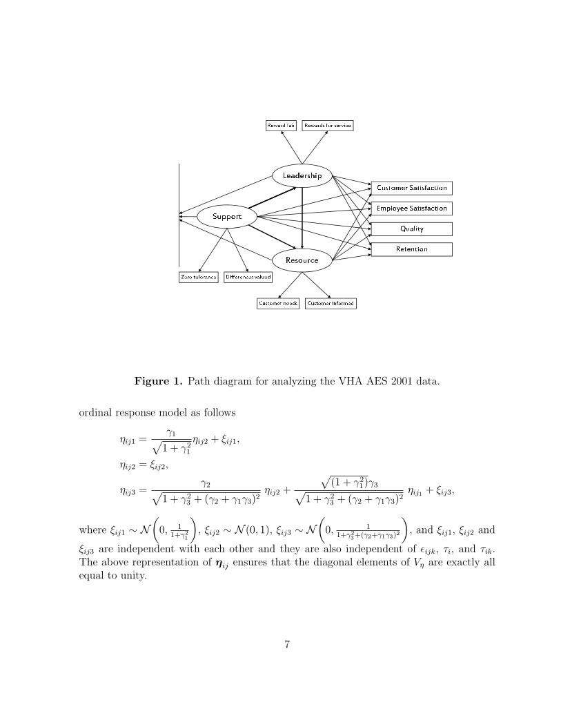
������ ���� ������� �� ������� �� ����� �������� ����� �!���"#$��%�& '�()�*�� ����� �!���"+��)��*, �%$�- .�� /0���1�� 2 ������1��� �03�� 4���"���"53�/6�� 1���� 53�/6�� �1��6��.�� /0���1�� 2 ������1��� �03��Figure 1. Path diagram for analyzing the VHA AES 2001 data.

ordinal response model as follows

ηij1 =γ1√

1 + γ21

ηij2 + ξij1,

ηij2 = ξij2,

ηij3 =γ2√

1 + γ23 + (γ2 + γ1γ3)2

ηij2 +

√(1 + γ2

1)γ3√1 + γ2

3 + (γ2 + γ1γ3)2ηij1 + ξij3,

where ξij1 ∼ N(

0, 11+γ2

1

), ξij2 ∼ N (0, 1), ξij3 ∼ N

(0, 1

1+γ23+(γ2+γ1γ3)2

), and ξij1, ξij2 and

ξij3 are independent with each other and they are also independent of εijk, τi, and τik.The above representation of ηij ensures that the diagonal elements of Vη are exactly allequal to unity.

7

As discussed in Section 2, there were missing values in both response variables yijk’sand covariates zijq’s. With the protection of the labor/management confidentiality agree-ment, it is unlikely that missing responses are due to the sensitive nature of questionsas the identification of individual respondents was not recorded. In addition, it does notappear that there were any apparent systematic patterns in the missing values of yijk’s orzijq’s in the AES 2001 data. Thus, it is reasonable to assume that any missingness in yijk

and covariates zijq is missing at random (MAR) (Rubin, 1976; Little and Rubin, 2002).As discussed in Ibrahim et al. (1999, 2005), we do not need to model the missing datamechanism for MAR missing responses and covariates. However, we need to model miss-ing covariates. To this end, we assume a series of one-dimensional distributions proposedby Lipsitz and Ibrahim (1996) for the missing covariate variables

f(zij1, zij2, . . . , zij,q|α)

=f(zijq|zij1, . . . , zij,q−1,αq)f(zij,q−1|zij,1, . . . , zij,q−2,αq−1) . . . f(zij1|α1), (3.9)

where αh is a vector of parameters for the hth conditional distribution, the α′hs are distinct,

and moreover, α = (α′1, . . . , α

′q)′, and extend θ to include α. Of course, for CC data, we

do not need to model the covariates.

Letting yij = (yij1, yij2, . . . , yijK)′, we thus partition the response vector y′ij into(y′ij,obs, y′ij,mis). Similarly, we partition the vector of covariates z′ij into (z′ij,obs, z

′ij,mis).

Let η = (η′ij, j = 1, 2, . . . , ni, i = 1, 2, . . . , I)′, τ = (τ1, τ2, . . . , τI)′, and τ ∗ = (τik, i =

1, 2, . . . , I, k = 1, 2, . . . , K)′. Also let Dobs = (yobs,zobs) denote the observed data, whereyobs = (y′ij,obs, j = 1, 2, . . . , ni, i = 1, 2, . . . , I)′ and zobs = (zij,obs, j = 1, 2, . . . , ni, i =1, 2, . . . , I)′. In addition, we introduce a missing indicator for the response in the data

δijk =

{1 if yijk is observed0 if yijk is missing

.

Thus, using the result for MAR missing responses given in Chen et al. (2008), thelikelihood function given Dobs can be written as

L(θ,y∗, τ , τ ∗|Dobs)

∝∫ I∏

i=1

{ ni∏j=1

[ K∏

k=1

(f(y∗ijk|µk, τi, τik, βk,ηij,φk, σ

2k,zij)1{λyijk−1 ≤ y∗ijk < λyijk

})δijk

]

× f(ηij|γ)f(zij,obs,zij,mis|α)}[ K∏

k=1

f(τik|σ2τ∗)

]f(τi|σ2

τ )dzmis, (3.10)

where y∗ = (y∗ijk, j = 1, 2, . . . , ni, i = 1, 2, . . . , I, k = 1, 2, . . . , K)′, 1{λyijk−1 ≤ y∗ijk <

8

λyijk} is the indicator function, zmis = (zij,mis, j = 1, 2, . . . , ni, i = 1, 2, . . . , I)′,

f(y∗ijk|µk, τi, τik,βk, ηij, φk, σ2k,zij)

=1√

2πσk

exp{− 1

2σ2k

[y∗ijk − (µk + τi + τik + β′kωkηij + φ′kzij)]

2}

,

f(τi|σ2τ ) = 1√

2πστexp

{− τ2i

2σ2τ

}, f(τik|σ2

τ∗) = 1√2πστ∗

exp{− τ2

ik

2σ2τ∗

}, and f(ηij|γ) = 1

(2π)r2 |Vη |

12

× exp{− 1

2η′ijV

−1η ηij

}.

4 Prior and Posterior Distributions

We take the joint prior for θ as

π(θ) = π(µ)π(β)π(φ)π(γ)π(σ2)π(σ2τ )π(σ2

τ∗)π(λ)π(α). (4.1)

The detailed specification for each prior on the right hand side of (4.1) is given as

follows: for location parameters, we take µkiid∼ N (µ0, σ

20), k = 1, 2, . . . , K, for π(µ),

βkiid∼ N (β0, Σβ0), k = 1, 2, . . . , K, for π(β), φk

iid∼ N (φ0, Σφ0), k = 1, 2, . . . , K, for π(φ),

and γliid∼ N (γ0, σ

20γ), l = 1, 2, . . . , r, for π(γ). For the scale parameters, we assume in-

verse gamma priors as follows: σ2k

iid∼ IG(a0, b0), k = 1, 2, . . . , K, for π(σ2), σ2τ ∼ IG(a1, b1)

for π(σ2τ ), and σ2

τ∗ ∼ IG(a2, b2) for π(σ2τ∗). For λ, we take π(λ) =

∏Kk=1 π(λk), where

π(λk) ∝ 1, which is a proper uniform over the constrained space defined by (3.4), fork = 1, 2, . . . , K. For π(α), we assume π(α) =

∏ql=1 π(α1), where the prior specification

for each π(α1) depends on the form of the one-dimensional conditional distribution forzijl.

Using (3.10) and (4.1), the joint posterior is thus given by

π(θ, y∗, τ , τ ∗|Dobs) ∝ L(θ,y∗, τ , τ ∗|Dobs)π(θ). (4.2)

Due to the complexity of the ordinal structural equation model and the presence of missingresponses and covariates, the analytical evaluation of the posterior distribution in (4.2)does not appear to be possible. However, the posterior distribution is computationallyattractive partially due to the use of the probit link, as an efficient Markov chain MonteCarlo (MCMC) sampling algorithm can be developed. The detailed steps of the MCMCsampling algorithm to sample from π(θ,y∗, τ , τ ∗|Dobs) is given in the Appendix.

9

5 Model assessment

For the ordinal response SEM developed in Section 3, we account for both facility effectsas well as covariate effects. We refer to this as the full model and denote it by M1. We areinterested in investigating how the exclusion of the two random effects terms introducedand the exclusion of covariates from M1 contribute to the fit of the data. Further, wewill investigate the exclusion from M1 in turns of the facility effects, then of the covariateeffects, and then the effect due to the exclusion of both the effects. The forms of thesemodels are given as follows:

M1 (Facility and covariates effects): y∗ijk = µk + τi + τik + β′kωkηij + φ′kzij + εijk;

M2 (Facility effect, no covariates): y∗ijk = µk + τi + τik + β′kωkηij + εijk;

M3 (No facility effect, but covariates effect): y∗ijk = µk + β′kωkηij + φ′kzij + εijk; and

M4 (Neither facility nor covariates effects): y∗ijk = µk + β′kωkηij + εijk.

We assess these four ordinal response models via the Bayesian Deviance InformationCriteria (DIC) proposed by Spiegelhalter et al. (2002). For model M1, we treat allfacility effects, τi and τik, and missing covariates, zij,mis, as parameters. Thus, we defineθ∗ = (θ, τ , τ ∗,zmis). The DIC measure proposed by Spiegelhalter et al. (2002) is givenby

DIC = D(θ∗) + 2pD, (5.1)

where D(θ∗) is a deviance function, θ∗ = E[θ∗|Dobs] is the posterior mean of θ∗, and pD

is the penalty due to model dimension and is evaluated as pD

= D(θ∗)−D(θ∗). For theordinal response SEM, the deviance function is defined as follows:

D(θ∗) = −2 logI∏

i=1

ni∏j=1

K∏

k=1

{Φ

(λk,yijk

− µ∗ijkσk

)− Φ

(λk,yijk−1 − µ∗ijk

σk

)}δijk

, (5.2)

where for the full model M1 with both facility random effects and covariate effects,µ∗ijk = µk + τi + τik +β′kωkηik +φ′

kzij. Using the extension to DIC as proposed by Huanget al. (2005) in the presence of missing covariates, we compute µ∗ijk = E(µ∗ijk|Dobs),

λkl = E(λkl|Dobs), σk = E(σk|Dobs), D(θ∗) = E[D(θ∗)|Dobs], and

D(θ∗) = −2 logI∏

i=1

ni∏j=1

K∏

k=1

{Φ

(λk,yijk

− µ∗ijkσk

)− Φ

(λk,yijk−1 − µ∗ijk

σk

)}δijk

.

The DIC measures are computed in a similar fashion for the other three competing models.The detail is omitted for brevity.

10

6 Analysis of the AES 2001 Ordinal Response Data

The VHA AES 2001 was an all employees survey conducted via self reported question-naire to ascertain organizational climate and locate intervention points, and was a followup to a previous VHA AES 1997. The main focus was on 4 outcome variable — Cus-tomer Satisfaction, Employee satisfaction, Quality and Retention, investigated via 3 workplace traits — Leadership, Support and Resource, which correspond to ηij1, ηij2, and ηij3,respectively. These traits being latent constructs, observed responses from the question-naire were identified that were considered as manifestations of the latent constructs. Thedimension of all the response (outcome + manifest) variables is K = 4 + 21 = 25, thenumber of latent traits is r = 3, while the number of facilities is I = 132. The loadingpattern of the 21 manifest variables was motivated by feedback from the field knowledgeof VHA, and further confirmed by factor analytic exploratory data analysis.

6.1 Specification of the model and priors

The dimensions of the vectors involved are as follows: for the single loading manifestvariables pk = 1, k = 1, . . . , 6. For the 15 manifest variables and 3 outcome variablespk = 3, k = 7, . . . , 25. The corresponding loading matrix are: ω1 = ω2 = (1, 0, 0)′;ω3 = ω4 = (0, 1, 0)′; ω5 = ω6 = (0, 0, 1)′ and ωk = I3, k = 7, . . . , 25; in the struc-tural part of the model, the dimension of the latent variable vector r = 3. The otherprior distributions have been described in Section 4. We specify the hyperparametersas follows. A N (0, 1000) or N (0, 1000I) prior is used for all location parameters in-cluding µk,βk,φk, γ1, γ2, and γ3. For the scale parameters, the hyperparameters area0 = a1 = a2 = 1 and b0 = b1 = b2 = 0.001. Since the outcome variable Retention (yij,25)is dichotomous, the cut-point is known.

For the covariates, since the zij’s are all dichotomized, the distributions for thesecovariates are specified as

f(zij1|α11) = αzij1

11 (1− α11)1−zij1 ,

f(zij2|zij1, α21, α22) =exp{zij2(α21 + α22zij1)}1 + exp(α21 + α22zij1)

,

f(zij3|zij1, zij2, α31, α32, α33) =exp{zij3(α31 + α32zij1 + α33zij2)}1 + exp(α31 + α32zij1 + α33zij2)

.

The prior distribution for α11 is Beta(0.001, 0.001), and the priors distributions of α21,α22, α31, α32, and α33 are all N (0, 1000) independently. Observe that all priors are non-informative.

11

6.2 Posterior Computation

In all the computations, we used 10,000 MCMC iterations, after a burn-in of 1000 iter-ations for each model, to compute all the posterior estimates, including posterior means(Estimates), posterior standard deviations (SDs), 95% highest posterior density inter-vals (HPDs) and DICs. The computer codes were written in FORTRAN 95 using IMSLsubroutines with double-precision accuracy. The convergence of the Gibbs sampler forall parameters has passed the recommendations of Cowles and Carlin (1996). The traceplots and auto-correlation plots all show good convergence and excellent mixing of theMCMC sampling algorithm.

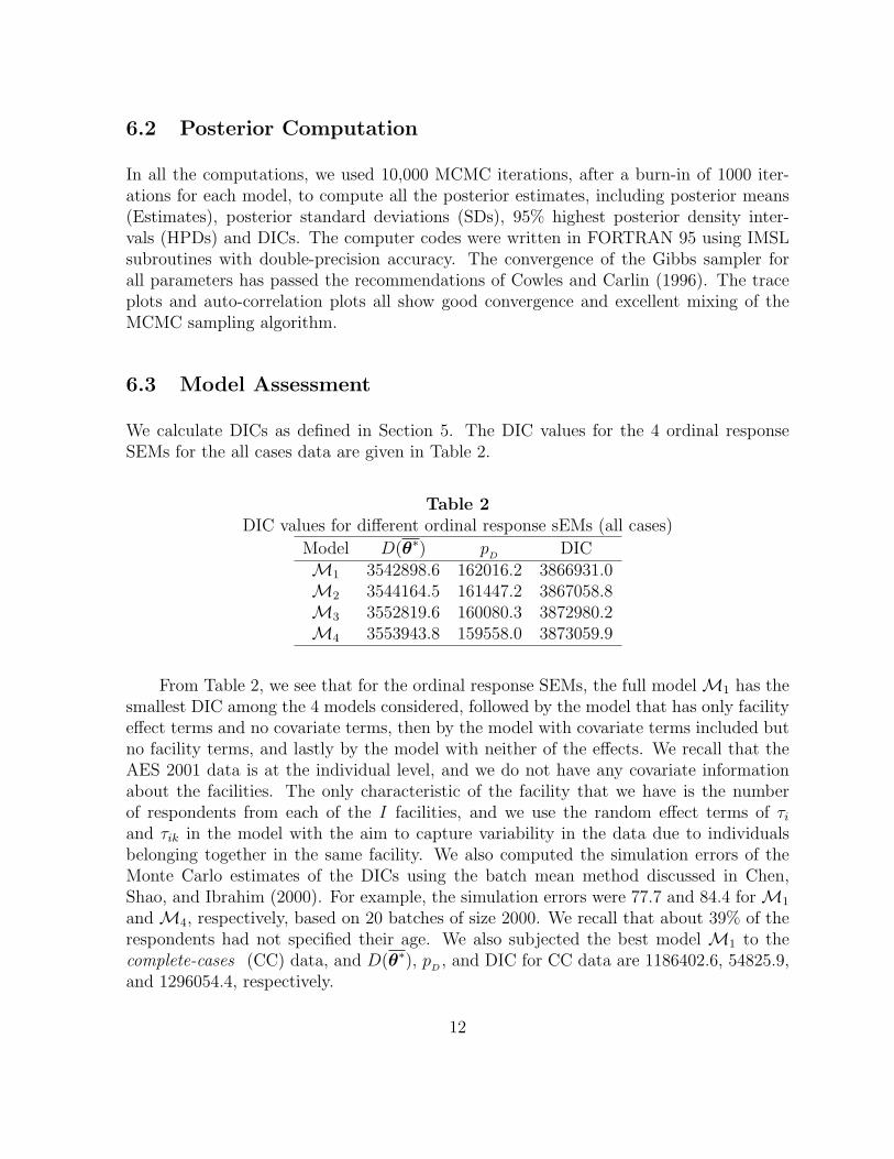
6.3 Model Assessment

We calculate DICs as defined in Section 5. The DIC values for the 4 ordinal responseSEMs for the all cases data are given in Table 2.

Table 2DIC values for different ordinal response sEMs (all cases)

Model D(θ∗) pD

DICM1 3542898.6 162016.2 3866931.0M2 3544164.5 161447.2 3867058.8M3 3552819.6 160080.3 3872980.2M4 3553943.8 159558.0 3873059.9

From Table 2, we see that for the ordinal response SEMs, the full model M1 has thesmallest DIC among the 4 models considered, followed by the model that has only facilityeffect terms and no covariate terms, then by the model with covariate terms included butno facility terms, and lastly by the model with neither of the effects. We recall that theAES 2001 data is at the individual level, and we do not have any covariate informationabout the facilities. The only characteristic of the facility that we have is the numberof respondents from each of the I facilities, and we use the random effect terms of τi

and τik in the model with the aim to capture variability in the data due to individualsbelonging together in the same facility. We also computed the simulation errors of theMonte Carlo estimates of the DICs using the batch mean method discussed in Chen,Shao, and Ibrahim (2000). For example, the simulation errors were 77.7 and 84.4 for M1

and M4, respectively, based on 20 batches of size 2000. We recall that about 39% of therespondents had not specified their age. We also subjected the best model M1 to thecomplete-cases (CC) data, and D(θ∗), p

D, and DIC for CC data are 1186402.6, 54825.9,

and 1296054.4, respectively.

12

6.4 Posterior Estimates

The direct effect and total effect are commonly used to describe the association betweentwo variables in the SEM. The direct effect is the direct path from one variable to theother, which is simply the coefficient βkj. The total effect takes into account the directionand all possible path coefficients between the two variables in the system (Bollen, 1987).If neither is exogenous, then total effect misses to capture the upstream effect due to otherconnected relationships in the model. To overcome the limitation of the total effect, Daset. al (2008) introduced the superbeta measure to capture the overall association betweenthe cause variable (either endogenous or exogenous) and the effect variable (endogenous).If the cause variable is exogenous, then the superbeta equals the corresponding total effect.For the ordinal response SEM, we use these measures to describe the association betweenlatent variables y∗ijk and ηij. Following from Das et. al (2008), the total effect betweeny∗ijk and ηij can be calculated as follows

βTy∗ijk,ηij

=

βk1 + βk3aγ3

b

βk1γ1

a+ βk2 + βk3

γ2+γ1γ3

b

βk3

where a =√

1 + γ21 , b =

√1 + γ2

3 + (γ2 + γ1γ3)2, and the superbeta between y∗ijk andηijr∗ , r∗ = 1, 2, 3, is given by

βsb(y∗ijk,ηij1) = Cov(y∗ijk, ηij1)/Var(ηij1) = βk1 + βk2

γ1

a+ βk3

[γ1γ2

ab+

γ3 a

b

],

βsb(y∗ijk,ηij2) = Cov(y∗ijk, ηij2)/Var(ηij2) = βk1

γ1

a+ βk2 + βk3

[γ2

b+

γ1γ3

b

],

and

βsb(y∗ijk,ηij3) = Cov(y∗ijk, η3)/Var(ηij3) = βk1

[γ1γ2

ab+

γ3a

b

]+ βk2

[γ2

b+

γ1γ3

b

]+ βk3.

In Table 3 (AC) and Table 4 (CC), we present the posterior estimates of directeffect, total effect, and superbeta corresponding to latent outcome variables y∗ijk, k =22, 23, 24, 25, α, γ, and σ2

τ and σ2τ∗ under the best model M1, where symbols used are

as follow — βk: direct effect; βTk : total effect; and βsb

k : superbeta. For the AC analy-sis (Table 3), based on the direct effect, we observe that Customer satisfaction is moststrongly directly associated with Resources, Quality is directly associated with Leader-ship and Resources, and Employee satisfaction and Retention are most directly associatedwith Leadership. Based on either the total effect or the superbeta, all four outcomes areassociated with Leadership, Support and Resource. However, based on the superbeta,

13

Leadership is most strongly associated with Employee satisfaction and Retention whileCustomer satisfaction is most strongly associated with Resources. These results suggestthat based on perception of service received, Resource in a facility is most important inimproving quality of service provided, while from the service provider perception, Lead-ership was the most important intervention area.

Table 3Posterior estimates of Model 1 (all cases)

Variable Estimate SD 95% HPD Variable Estimate SD 95% HPDCustomer satisfaction Quality

β22,1 0.019 0.0023 ( 0.014, 0.023) β24,1 0.112 0.0030 (0.107, 0.118)βT

22,1 0.089 0.0021 ( 0.084, 0.093) βT24,1 0.162 0.0026 (0.157, 0.167)

βsb22,1 0.134 0.0017 ( 0.131, 0.137) βsb

24,1 0.210 0.0022 (0.206, 0.215)β22,2 0.037 0.0019 ( 0.033, 0.040) β24,2 0.057 0.0024 (0.053, 0.062)βT

22,2 0.131 0.0016 ( 0.128, 0.134) βT24,2 0.178 0.0021 (0.174, 0.182)

βsb22,2 0.131 0.0016 ( 0.128, 0.134) βsb

24,2 0.178 0.0021 (0.174, 0.182)β22,3 0.182 0.0023 ( 0.178, 0.187) β24,3 0.128 0.0031 (0.122, 0.134)βT

22,3 0.182 0.0023 ( 0.178, 0.187) βT24,3 0.128 0.0031 (0.122, 0.134)

βsb22,3 0.209 0.0017 ( 0.206, 0.212) βsb

24,3 0.213 0.0025 (0.208, 0.218)Employee satisfaction Retention

β23,1 0.195 0.0027 ( 0.190, 0.200) β25,1 0.298 0.0083 (0.282, 0.314)βT

23,1 0.232 0.0023 ( 0.228, 0.237) βT25,1 0.324 0.0072 (0.310, 0.339)

βsb23,1 0.258 0.0018 ( 0.254, 0.262) βsb

25,1 0.375 0.0059 (0.364, 0.386)β23,2 0.023 0.0021 ( 0.018, 0.027) β25,2 0.076 0.0074 (0.062, 0.090)βT

23,2 0.174 0.0018 ( 0.170, 0.177) βT25,2 0.271 0.0058 (0.259, 0.282)

βsb23,2 0.174 0.0018 ( 0.170, 0.177) βsb

25,2 0.271 0.0058 (0.259, 0.282)β23,3 0.096 0.0028 ( 0.091, 0.102) β25,3 0.068 0.0083 (0.051, 0.084)βT

23,3 0.096 0.0028 ( 0.091, 0.102) βT25,3 0.068 0.0083 (0.051, 0.084)

βsb23,3 0.209 0.0022 ( 0.204, 0.213) βsb

25,3 0.259 0.0064 (0.246, 0.271)α11 -2.224 0.0197 (-2.261, -2.184) σ2

τ 0.002 0.0002 (0.001, 0.002)α21 0.506 0.0288 ( 0.447, 0.561) σ2

τ∗ 0.001 0.0001 (0.001, 0.001)α22 0.385 0.0019 ( 0.382, 0.389) γ1 0.656 0.0067 (0.642, 0.669)α31 0.940 0.0114 ( 0.918, 0.963) γ2 0.303 0.0076 (0.289, 0.318)α32 1.431 0.0463 ( 1.339, 1.521) γ3 0.390 0.0072 (0.376, 0.404)α33 -0.139 0.0182 (-0.175, 0.104)

For the CC analysis (Table 4), we observe that for almost all the β coefficients, theCC estimates for the full model M1 are larger than the AC estimates. The β coefficientsbetween outcome variables and Resource are smaller in the AC analysis compared to theAC analysis. But for the superbeta measure, all the CC estimates are stronger than in theAC case. On the other hand, for the γ coefficients, the γ1 and γ3 coefficients between latent

14

variables ‘Leadership’ and ‘Support’ and between ‘Resource’ and ‘Leadership’ significantlyincrease for the complete cases from the all cases.

Table 4Posterior estimates of Model 1 (complete cases)

Variable Estimate SD 95% HPD Variable Estimate SD 95% HPDCustomer satisfaction Quality

β22,1 0.037 0.0039 (0.029, 0.044) β24,1 0.148 0.0054 (0.138, 0.159)βT

22,1 0.112 0.0036 (0.105, 0.119) βT24,1 0.199 0.0047 (0.190, 0.208)

βsb22,1 0.155 0.0028 (0.150, 0.161) βsb

24,1 0.243 0.0038 (0.235, 0.250)β22,2 0.033 0.0031 (0.027, 0.039) β24,2 0.046 0.0042 (0.038, 0.055)βT

22,2 0.140 0.0026 (0.135, 0.145) βT24,2 0.193 0.0036 (0.186, 0.199)

βsb22,2 0.140 0.0026 (0.135, 0.145) βsb

24,2 0.193 0.0036 (0.186, 0.199)β22,3 0.174 0.0039 (0.166, 0.182) β24,3 0.119 0.0054 (0.108, 0.129)βT

22,3 0.174 0.0039 (0.166, 0.182) βT24,3 0.119 0.0054 (0.108, 0.129)

βsb22,3 0.211 0.0028 (0.205, 0.216) βsb

24,3 0.226 0.0042 (0.217, 0.233)Employee satisfaction Retention

β23,1 0.222 0.0046 (0.213, 0.231) β25,1 0.342 0.0153 (0.312, 0.373)βT

23,1 0.259 0.0039 (0.251, 0.266) βT25,1 0.357 0.0133 (0.331, 0.383)

βsb23,1 0.280 0.0030 (0.275, 0.286) βsb

25,1 0.411 0.0105 (0.390, 0.431)β23,2 0.016 0.0037 (0.009, 0.024) β25,2 0.082 0.0127 (0.056, 0.106)βT

23,2 0.191 0.0031 (0.184, 0.196) βT25,2 0.303 0.0100 (0.283, 0.322)

βsb23,2 0.191 0.0031 (0.184, 0.196) βsb

25,2 0.303 0.0100 (0.283, 0.322)β23,3 0.085 0.0047 (0.076, 0.094) β25,3 0.035 0.0145 (0.007, 0.064)βT

23,3 0.085 0.0047 (0.076, 0.094) βT25,3 0.035 0.0145 (0.007, 0.064)

βsb23,3 0.219 0.0036 (0.212, 0.226) βsb

25,3 0.270 0.0110 (0.248, 0.291)γ1 0.744 0.0121 (0.721, 0.768) σ2

τ 0.002 0.0003 (0.002, 0.003)γ2 0.292 0.0135 (0.265, 0.318) σ2

τ∗ 0.001 0.0001 (0.001, 0.001)γ3 0.430 0.0128 (0.406, 0.456)

6.5 Normal-Ordinal SEMs

As discussed in Bollen (1989), the Pearson correlation coefficients between categoricalmeasures are generally less than the correlation of the corresponding continuous variables.This phenomenon may more likely occur with few categories (e.g., < 5). However, asthe number of categories increases and the marginal distributions become similar, thedifference in correlations lessens. For the AES 2001 data, the first 21 manifest variablesare ordinal with 5 levels and the last four are the outcome variables with Retentionbeing the binary response variable. It is of practical interest to investigate whether thestructural part of the SEM and the loading coefficients of the last four measurement partof the ordinal response SEM are sensitive to the specification of the marginal distributions

15

of yijk for k = 1, 2, . . . , 21 for the first 21 manifest variables. Specifically, we assume thaty∗ijk = yijk in (3.3) for k = 1, 2, . . . , 21. That is, we assume the normal distribution modelsdirectly for the ordinal responses from the first 21 manifest variables. As the last fouroutcome variables are of primary interest, we still assume the ordinal (binary) models forthese four outcome variables. Under these assumptions, the resulting SEM is called thenormal-ordinal SEM.

First, we compare the four variations of the normal-ordinal SEM discussed in Section5 via DIC. Similar to (5.2), the deviance function for the normal-ordinal SEM is given by

D(θ∗) = −2I∑

i=1

ni∑j=1

{21∑

k=1

δijk

[− 1

2log(2πσ2

k)−1

2σ2k

(yijk − µ∗ijk

)2]

+K∑

k=22

δijk log[Φ

(λk,yijk− µ∗ijk

σk

)− Φ

(λk,yijk−1 − µ∗ijkσk

)]},

where for the full model M1 with both facility random effects and covariate effects,µ∗ijk = µk +τi +τik +β′kωkηik +φ′

kzij. For the all cases AES 2001 data, under the normal-ordinal SEMs, the DIC values are 4214927.9, 4214942.2, 4220289.6, and 4220339.3 forM1, M2, M3, and M4, respectively. Thus, the best normal-ordinal SEM is M1, thesecond best DIC normal-ordinal SEM is M2, and the worst DIC normal-ordinal SEM isM4. Although the DIC values under the normal-ordinal SEMs are not comparable tothose under the ordinal SEMs (Table 2), the orders of these four DIC values under thesetwo types of SEMs are the same.

Next, we compute the posterior estimates of direct effect, total effect, and superbetacorresponding to latent outcome variables y∗ijk, k = 22, 23, 24, 25, α, γ, and σ2

τ and σ2τ∗

under the best normal-ordinal model M1 and the results are shown in Table 5 (AC) andTable 6 (CC). Comparing the results in Table 5 to those in Table 3, we observe that thesetwo sets of the posterior estimates of direct effect, total effect, superbeta, and γ are verysimilar, and the estimates of α are almost identical. However, the posterior estimates ofσ2

τ and σ2τ∗ under the normal-ordinal SEM (Table 5) are much larger than those under the

ordinal SEM (Table 3). The similar patterns are observed when we compare the resultsin Table 6 to those in Table 4 for the CC data.

16

Table 5Posterior estimates of Model 1 (all cases) under the normal-ordinal SEM

Variable Estimate SD 95% HPD Variable Estimate SD 95% HPDCustomer satisfaction Quality

β22,1 0.017 0.0023 ( 0.012, 0.021) β24,1 0.113 0.0030 (0.107, 0.119)βT

22,1 0.088 0.0021 ( 0.084, 0.092) βT24,1 0.163 0.0026 (0.158, 0.168)

βsb22,1 0.128 0.0017 ( 0.125, 0.132) βsb

24,1 0.203 0.0022 (0.199, 0.207)β22,2 0.031 0.0018 ( 0.028, 0.035) β24,2 0.046 0.0022 (0.042, 0.050)βT

22,2 0.122 0.0015 ( 0.119, 0.125) βT24,2 0.163 0.0019 (0.159, 0.167)

βsb22,2 0.122 0.0015 ( 0.119, 0.125) βsb

24,2 0.163 0.0019 (0.159, 0.167)β22,3 0.185 0.0023 ( 0.181, 0.189) β24,3 0.127 0.0031 (0.122, 0.134)βT

22,3 0.185 0.0023 ( 0.181, 0.189) βT24,3 0.127 0.0031 (0.122, 0.134)

βsb22,3 0.207 0.0017 ( 0.204, 0.211) βsb

24,3 0.206 0.0024 (0.201, 0.210)Employee satisfaction Retention

β23,1 0.189 0.0026 ( 0.184, 0.194) β25,1 0.293 0.0083 (0.277, 0.310)βT

23,1 0.229 0.0022 ( 0.224, 0.233) βT25,1 0.325 0.0072 (0.311, 0.339)

βsb23,1 0.250 0.0018 ( 0.247, 0.254) βsb

25,1 0.376 0.0059 (0.365, 0.388)β23,2 0.017 0.0020 ( 0.013, 0.021) β25,2 0.075 0.0069 (0.062, 0.089)βT

23,2 0.164 0.0017 ( 0.160, 0.167) βT25,2 0.270 0.0056 (0.259, 0.280)

βsb23,2 0.164 0.0017 ( 0.160, 0.167) βsb

25,2 0.270 0.0056 (0.259, 0.280)β23,3 0.102 0.0027 ( 0.097, 0.107) β25,3 0.083 0.0081 (0.067, 0.099)βT

23,3 0.102 0.0027 ( 0.097, 0.107) βT25,3 0.083 0.0081 (0.067, 0.099)

βsb23,3 0.206 0.0021 ( 0.202, 0.210) βsb

25,3 0.266 0.0063 (0.254, 0.278)α11 -2.226 0.0202 (-2.266, -2.187) σ2

τ 0.006 0.0009 (0.005, 0.008)α21 0.508 0.0293 ( 0.451, 0.565) σ2

τ∗ 0.006 0.0002 (0.005, 0.006)α22 0.385 0.0018 ( 0.382, 0.389) γ1 0.639 0.0065 (0.627, 0.652)α31 0.941 0.0113 ( 0.918, 0.963) γ2 0.279 0.0073 (0.265, 0.293)α32 1.433 0.0457 ( 1.343, 1.522) γ3 0.390 0.0073 (0.375, 0.404)α33 -0.139 0.0180 (-0.175, -0.104)

7 Discussion

In this paper, we have carried out an extensive investigation of the ordinal response SEM.We have shown that the use of latent variables linking the unobserved continuous variablesy∗ijk’s to the observed ordinal or binary response variables yijk’s is a useful modelingtechnique, which facilitates an easy implementation of the posterior computation andprovides a great flexibility to incorporate different types of responses such as continuous,ordinal, and binary responses in the survey data. For the AES 2001 data, we have observedthat the ordinal SEM with both facility level random effect terms as well as individualcovariates fits the data best based on the DIC measure even though it has the largestpenalty for dimensionality. Also, including facility random effect terms is more important

17

than including just covariate information, implying that variability within facilities ismore pronounced than variability in terms of demographic variables within individuals.This finding confirms that facility characteristics differ not only in size but also in theavailable service resources, and responses by individuals belonging to different facilitiesare bound to reflect that. In fact, including facility random effects captures the naturalheterogeneity because of the clustering of individuals into specific facilities. We note thatthe similar results were also obtained by Das et al. (2008) based on the VHA AES 1997data.

Table 6Posterior estimates of Model 1 (complete cases) under the normal-ordinal SEM

Variable Estimate SD 95% HPD Variable Estimate SD 95% HPDCustomer satisfaction Quality

β22,1 0.032 0.0048 (0.025, 0.040) β24,1 0.145 0.0052 (0.134, 0.155)βT

22,1 0.109 0.0035 (0.101, 0.115) βT24,1 0.197 0.0046 (0.188, 0.206)

βsb22,1 0.147 0.0027 (0.142, 0.153) βsb

24,1 0.233 0.0037 (0.226, 0.241)β22,2 0.027 0.0029 (0.021, 0.033) β24,2 0.035 0.0039 (0.028, 0.043)βT

22,2 0.130 0.0024 (0.125, 0.135) βT24,2 0.177 0.0034 (0.171, 0.184)

βsb22,2 0.130 0.0024 (0.125, 0.135) βsb

24,2 0.177 0.0034 (0.171, 0.184)β22,3 0.179 0.0038 (0.172, 0.187) β24,3 0.123 0.0051 (0.114, 0.133)βT

22,3 0.179 0.0038 (0.172, 0.187) βT24,3 0.123 0.0051 (0.113, 0.133)

βsb22,3 0.210 0.0027 (0.205, 0.215) βsb

24,3 0.219 0.0040 (0.212, 0.228)Employee satisfaction Retention

β23,1 0.211 0.0045 (0.202, 0.219) β25,1 0.327 0.0149 (0.299, 0.357)βT

23,1 0.251 0.0039 (0.244, 0.259) βT25,1 0.351 0.0127 (0.328, 0.378)

βsb23,1 0.270 0.0030 (0.264, 0.276) βsb

25,1 0.409 0.0101 (0.390, 0.429)β23,2 0.012 0.0034 (0.005, 0.018) β25,2 0.085 0.0119 (0.062, 0.108)βT

23,2 0.180 0.0030 (0.174, 0.186) βT25,2 0.303 0.0095 (0.285, 0.323)

βsb23,2 0.180 0.0030 (0.174, 0.186) βsb

25,2 0.303 0.0095 (0.285, 0.323)β23,3 0.096 0.0045 (0.087, 0.105) β25,3 0.059 0.0143 (0.030, 0.086)βT

23,3 0.096 0.0045 (0.087, 0.105) βT25,3 0.059 0.0143 (0.030, 0.086)

βsb23,3 0.218 0.0035 (0.211, 0.225) βsb

25,3 0.279 0.0108 (0.258, 0.301)γ1 0.721 0.0118 (0.698, 0.744) σ2

τ 0.004 0.0006 (0.002, 0.005)γ2 0.270 0.0130 (0.244, 0.295) σ2

τ∗ 0.004 0.0002 (0.003, 0.004)γ3 0.425 0.0123 (0.400, 0.448)

In Section 6, we have empirically shown that treating the categorical responses as or-dinal or continuous for the 21 manifest variables results in very similar posterior estimatesof the loading coefficients for the 4 ordinal/binary outcome variables in the measurementpart of the SEM and the parameters in the structural part of the SEM. We have alsoobserved that the same best DIC model is obtained under both the ordinal SEMs andthe normal-ordinal SEMs. Interestingly, such treatment of the categorical responses for

18

the manifest variables does not at all affect the posterior estimates of parameters in themissing covariates models.

Finally, we mention that in the ordinal SEM, the probit links were used for all ordinalor binary responses. As discussed in Chen, Dey, and Shao (1999) and Kim, Chen, and Dey(2008), the choice of links is important in fitting categorical response data. However, theliterature on the importance of the choice of links in the structural equations framework isstill sparse. In addition, in this paper, we assume that missing responses and/or missingcovariates are missing at random. This assumption needs to be further examined. Theseimportant issues are currently under investigation.

Appendix: Posterior Computation

To implement the MCMC sampling algorithm, we need to sample from the followingconditional posterior distributions in turn:

(i) [y∗,λ|β,φ,σ2, τ , τ ∗,η, zmis, Dobs];

(ii) [µ|y∗,β,φ,σ2, τ , τ ∗, η, zmis, Dobs];

(iii) [σ2|y∗,µ,β, φ, τ , τ ∗,η,zmis, Dobs];

(iv) [β|y∗,µ, φ,σ2, τ , τ ∗,η, zmis, Dobs];

(v) [φ|y∗,β,σ2, τ , τ ∗,η,zmis, Dobs];

(vi) [σ2τ |τ , Dobs];

(vii) [σ2τ∗|τ ∗, Dobs];

(viii) [η|y∗,µ,β,φ, γ, σ2, τ , τ ∗, zmis, Dobs];

(ix) [τ |y∗,µ, β,φ,σ2, σ2τ , τ

∗,η, zmis, Dobs];

(x) [τ ∗|y∗,µ, β,φ,σ2, σ2τ∗ , τ , η, zmis, Dobs];

(xi) [γ|η, Dobs];

(xii) [α|zmis, Dobs]; and

(xiii) [zmis|µ,β, φ,σ2, τ , τ ∗,η,α, Dobs].

19

We briefly discuss how we sample from each of the above posterior conditional distri-butions. For (i), we apply the collapsed Gibbs technique of Liu (1994) via the followingidentity:

[y∗,λ|β,φ,σ2, τ , τ ∗,η,zmis, Dobs] = [λ|β,φ,σ2, τ , τ ∗,η, zmis, Dobs]

× [y∗|λ, β,φ,σ2, τ , τ ∗,η, zmis, Dobs].

That is, we sample λ after collapsing out y∗. It can be shown that given β,φ,σ2, τ , τ ∗,η,zmis, and Dobs, λk’s are conditionally independent. Thus, we can sample each λk inde-pendently. Instead of directly sampling λk, we use the “de-constrained” transformationfor the Metropolis-Hastings algorithm proposed by Chen and Dey (2000b) as follows

λkl =λk,l−1 + exp(ζkl)

1 + exp(ζkl),

where −∞ < ζkl < ∞, l = 2, . . . , Lk − 2. Let π(λk|β, φ,σ2, τ , τ ∗,η,zmis, Dobs) denotethe conditional distribution of λk. Then, the conditional distribution of ζk = (ζkl, l =2, . . . , Lk − 2)′ is obtained by

π(ζk|β,φ, σ2, τ , τ ∗, η,zmis, Dobs)

∝ π(λk|β, φ, σ2, τ , τ ∗, η,zmis, Dobs)

Lk−2∏

l=2

(1− λk,l−1) exp(ζkl)

[1 + exp(ζkl)]2.

Let ζk = argmaxζklog π(ζk|β,φ,σ2, τ , τ ∗,η, zmis, Dobs) and Σζk

is minus the inverse ma-

trix of the second derivative of log π(ζk|β,φ, σ2, τ , τ ∗,η,zmis, Dobs) evaluated at ζ = ζk.We then sample ζk via the standard Metropolis algorithm using the proposal N (ζk, Σζk

).Since the conditional distribution of y∗ijk is a truncated normal, N (µk+τi+τik+β′kωkηij +φ′

kzij, σ2k)1{λyijk−1 ≤ y∗ijk < λyijk

}, sampling y∗ijk is straightforward. Note that whenδijk = 0, we do not need to sample y∗ijk.

For (ii), given y∗,β, φ,γ,σ2, τ , τ ∗,η,zmis, Dobs, the µk are conditionally independentand

µk|y∗,β, φ,σ2, τ , τ ∗,η,zmis, Dobs

∼ N( ∑I

i=1

∑nij=1 δijk(y∗ijk−τi−τik−β′

kωkηij−φ′kzij)

σ2k

+ µ0

σ20∑I

i=1

∑nij=1 δijk

σ2k

+ 1σ20

,1

∑Ii=1

∑nij=1 δijk

σ2k

+ 1σ20

),

20

for k = 1, 2, . . . , K. For (iii), again the σ2k are conditionally independent and distributed

as

σ2k|y∗,µ,β,φ, τ , τ ∗, η,zmis, Dobs

∼ IG(

I∑i=1

ni∑j=1

δijk

2+ a0,

∑i

∑j

δijk[y∗ijk − (µk + τi + τik + β′kωkηij + φ′

kzij)]2

2+ b0

),

for k = 1, 2, . . . , K − 1. For (iv), we have

βk | y∗,µ,φ,σ2, τ , τ ∗,η, zmis ∼ Npk(B−1

βk

Aβk, B−1

βk

)

for k = 1, 2, . . . , K, where Aβk= 1

σ2k

∑Ii=1

∑ni

j=1 ωkηijδijk(y∗ijk − µk − τi − τik − φ′

kzij) +

Σ−10 β0 and Bβk

= 1σ2

kωk

[ ∑Ii=1

∑ni

j=1 ηijη′ij

]ω′

k + Σ−10 . For (v),

φk | y∗, β,σ2, τ , τ ∗,η, zmis, Dobs ∼ Nq(B−1

φk

Aφk, B−1

φk

),

where

Aφk=

1

σ2k

I∑i=1

ni∑j=1

(y∗ijk − µk − τi − τik − β′kωkηij)zij + Σ−1φ0

φ0

and Bφk= 1

σ2k

∑Ii=1

∑ni

j=1 zijz′ij + Σ−1

φ0. For (vi)

σ2τ | τ , Dobs ∼ IG

(a1 +

I

2,

1

2

I∑i=1

τ 2i + b1

),

and for (vii)

σ2τ∗|τ ∗, Dobs ∼ IG

(IK

2+ a2,

∑i

∑k τ 2

ik

2+ b2

).

For the latent variables in (viii),

ηij|y∗,µ, β,φ,γ,σ2, τ , τ ∗,zmis, Dobs ∼ Nr(B−1ηij

Aηij, B−1

ηij),

where Aηij=

∑Kk=1

[1σ2

kω′

kβkδijk(y∗ijk−µk−τi−τik−φ′

kzij)]

and Bηij=

∑Kk=1

[δijk

σ2k

ω′kβkβ

′kωk

]

+V −1η . For (ix), the τi are conditionally independent and distributed as

τi | y∗, µ,β,φ,σ2, σ2τ , τ

∗,η,zmis, Dobs

∼ N(∑ni

j=1

∑Kk=1 δijk(y

∗ijk − µk − τik − β′kωkηij − φ′

kzij)/σ2k∑ni

j=1

∑Kk=1

δijk

σ2k

+ 1σ2

τ

,1∑ni

j=1

∑Kk=1

δijk

σ2k

+ 1σ2

τ

),

21

and for (x),

τik | y∗,µ,β,φ, σ2, σ2τ∗ , τ ,η,zmis, Dobs

∼ N(∑ni

j=1 δijk(y∗ijk − µk − τi − β′kωkηij − φ′

kzij)

σ2k(

∑nij=1 δijk

σ2k

+ 1σ2

τ∗)

,1

∑nij=1 δijk

σ2k

+ 1σ2

τ∗

).

The conditional distributions for (ii) to (x) are either normal or inverse gamma distribu-tions and therefore, sampling from these distributions is straightforward.

For (xi), we use the localized Metropolis algorithm discussed in Chen, Shao, andIbrahim (2000, Chapter 2) to sample γ from [γ|η, Dobs]. Let

π∗(γ|η, Dobs) =[ I∏

i=1

ni∏j=1

|Vη|−1/2 exp{− 1

2η′ijV

−1η ηij

}]π(γ),

where π(γ) is the prior for γ. We compute

γ = argmaxγ1,γ2,γ3

log π∗(γ|η, Dobs) and Σ =

[− ∂2 log π∗(γ|η, Dobs)

∂γi∂γj

∣∣∣∣∣γ=γ

]−1

.

We use N (γ, c∗Σ) as the proposed density for the localized Metropolis algorithm, wherec∗ is a tuning parameter.

For (xii), π(α|zmis, Dobs) ∝[ ∏I

i=1

∏ni

j=1 f(zij,obs, zij,mis|α)]π(α). For various covari-

ate distributions specified through a series of one dimensional conditional distributions,sampling α is straightforward. For (xiii), given µ, β,φ,σ2, τ , τ ∗,η, α, and Dobs, zij,mis’sare independent across all i and j, and the conditional distribution for zij,mis is

π(zij,mis|µ, β,φ,σ2, τ , τ ∗,η, α, Dobs)

∝K∏

k=1

{Φ

(λk,yijk− µ∗ijk

σk

)− Φ

(λk,yijk−1 − µ∗ijkσk

)}δijk

f(zij,obs,zij,mis|α),

where µ∗ijk = µk + τi + τik +β′kωkηik +φ′kzij. Thus, sampling zmis depends on the form of

f(zij,obs,zij,mis|α). For the VHA AES 2001 data, π(zij,mis|µ,β,φ,σ2, τ , τ ∗,η,α, Dobs)is simply a multinomial distribution, which is easy to sample from.

Acknowledgments

The authors wish to thank the Guest Editor and a referee for helpful comments which haveled to an improvement of this article. The authors also wish to acknowledge and thank the

22

Veterans Health Administration and the National Center for Organizational Developmentfor access to the All Employee Survey (AES) 2001 data and their substantial efforts toinsure the quality and integrity of these data. Dr. Kim’s research is supported by theIntramural Research Program of the Eunice Kennedy Shriver National Institute of ChildHealth and Human Development; National Institutes of Health. Dr. Chen’s research waspartially supported by NIH grants #GM 70335 and #CA 74015 and a Faculty LargeResearch Grant from University of Connecticut. Dr. Warren’s research was funded bythe VHA National Center for Organizational Development.

References

Albert, J. H. (1992). Bayesian estimation of normal ogive item response curves usingGibbs sampling. J. Educ. Statist. 17:251-269.

Albert, J. H., Chib, S. (1993). Bayesian analysis of binary and polychotomous responsedata. J. Amer. Statist. Assoc. 88:669-679.

Arminger, G., Muthen, B. O. (1998). A Bayesian approach to nonlinear latent variablemodels using the Gibbs sampler and the Metropolis-Hastings algorithm. Psychome-trika 63:271-300.

Bollen, K. A. (1987). Total, direct, and indirect effects in structural equation models.Sociolog. Methodol. 17:37-69.

Bollen, K. A. (1989). Structural Equations with Latent Variables. New York: Wiley.

Branden-Roche, K., Miglioretti, D., Zeger, S., Rathouz, P. (1997). Latent variableregression for multiple discrete outcomes. J. Amer. Statist. Assoc. 92:1375-1386.

Chen, C.-F. (1981). The EM approach to the multiple indicators and multiple causesmodel via the estimation of the latent variable. J. Amer. Statist. Assoc. 76:704-708.

Chen, M.-H., Dey, D. K. (1998). Bayesian modeling of correlated binary responses viascale mixture of multivariate normal link functions. Sankhya, Ser. A, 60:322-343.

Chen, M.-H., Dey, D. K. (2000a). Bayesian data analysis of longitudinal binary responsemodels. In Ghosh, J.K., Sen, P.K., Sinha, B.K., eds. Proceedings of the ThirdInternational Triennial Calcutta Symposium on Probability and Statistics. Oxford:Oxford University Press, pp. 100-123.

Chen, M.-H., Dey, D. K. (2000b). A unified Bayesian analysis for correlated ordinal datamodels. Brazilian J. Probab. Statist. 14:87-111.

23

Chen, M.-H., Dey, D. K., Shao, Q.-M. (1999). A new skewed link model for dichotomousquantal response data. J. Amer. Statist. Assoc. 94:1172-1186.

Chen, M.-H., Shao, Q.-M., Ibrahim, J. G. (2000). Monte Carlo Methods in BayesianComputation. New York: Springer-Verlag.

Chen, Q., Ibrahim, J.G., Chen, M.-H., and Senchaudhuri, P. (2008). Theory and in-ference for regression models with missing response and covariates. J. MultivariateAnal. 99:1302-1331.

Chib, S., Greenberg, E. (1998). Analysis of multivariate probit models. Biometrika85:347-361.

Cowles, C., Carlin, B. P. (1996). Markov chain Monte Carlo convergence diagnostics: Acomparative review. J. Amer. Statist. Assoc. 91:883-904.

Das, S., Chen, M.-H., Kim, S., Warren, N. (2008), A Bayesian structural equationsmodel for multilevel data with missing responses and missing covariates. BayesianAnalysis 3:197-224.

Eaton, W. W., Bohrnstedt, G. (1989). Introduction to latent variable models for dichoto-mous outcomes: analysis of data from the epidemiologic catchment area program.Sociolog. Methods Research 18:4-18.

Hagenaars, J. A. (1990). Categorical Longitudinal Data - Log-Linear Analysis of Panel,Trend and Cohort Data. Newbury Park: Sage.

Hatcher, L. (2000). A Step-by-Step Approach to Using the SAS System for Factor Anal-ysis and Structural Equation Modeling. Cary, NC: SAS Institute Inc.

Huang, L., Chen, M.-H., Ibrahim, J. G. (2005). Bayesian analysis for generalized linearmodels with nonignorably missing covariates. Biometrics 61:767-780.

Ibrahim, J. G., Chen, M.-H., Lipsitz, S. R., Herring, A. H. (2005). Missing data methodsin regression models. J. Amer. Statist. Assoc. 100:332-346.

Ibrahim, J. G., Lipsitz, S. R., Chen, M.-H. (1999). Missing covariates in generalizedlinear models when the missing data mechanism is nonignorable. J. Roy. Statist.Soc., Ser. B 61:173-190.

Kim, S., Chen, M.-H., Dey, D. K. (2008). Flexible generalized t-link models for binaryresponse data. Biometrika 95:93-106.

Lee, S.-Y., Poon, W.-Y., Bentler, P. M. (1992). Structural equation models with contin-uous and polytomous variables. Psychometrika 57:89-105.

24

Li, F., Harmer, P., Duncan, T. E., Duncan, S. C., Acock, A., Boles, S. (1998). Ap-proaches to testing interaction effects using structural equation modeling method-ology. Multivariate Behavioral Research 33:1-39.

Lipsitz, S. R., Ibrahim, J. G. (1996). A conditional model for incomplete covariates inparametric regression models. Biometrika 83:916-922.

Little, R. J. A., Rubin, D. B. (2002). Statistical Analysis with Missing Data. SecondEdition. New York: John Wiley.

Liu, J. S. (1994). The collapsed Gibbs sampler in Bayesian computations with applica-tions to a gene regulation problem. J. Amer. Statist. Assoc. 89:958-966.

McCullagh, P., Nelder, J. A. (1989). Generalized Linear Models. London: Chapman &Hall.

Meredith, W., Millsap, R. E. (1992). On the misuse of manifest variables in the detectionof measurement bias. Psychometrika 57:289-311

Nandram, B. and Chen, M.-H. (1996). Accelerating Gibbs sampler convergence in thegeneralized linear models via a reparameterization. J. Statist. Comput. Simul.54:129-144.

Olsson, U. (1979). Maximum likelihood estimation of the polychoric correlation. Psy-chometrika 44:443-460.

Rubin, D. B. (1976). Inference and missing data. Biometrika 63:581-592.

Skrondal, A., Rabe-Hesketh, S. (2005). Structural equation modeling: categorical vari-ables. In Everitt, B., Howell, D., eds., Encyclopedia of Statistics in BehavioralScience. New York: Wiley, pp. 2352.

Spiegelhalter, D. J., Best, N. G., Carlin., B. P., van der Linde, A. (2002). Bayesianmeasures of model complexity and fit. J. Roy. Statist. Soc., Ser. B 62:583-639.

Zhu, H. T., Lee, S. Y. (1999). Statistical analysis of nonlinear factor analysis models.British J. Mathemat. Statist. Psychology 52:225-242.

25