Computational Ecology and Software, 2014, 4(1)
85
Computational Ecology and Software Vol. 4, No. 1, 1 March 2014 International Academy of Ecology and Environmental Sciences
Transcript of Computational Ecology and Software, 2014, 4(1)

Computational Ecology and Software
Vol. 4, No. 1, 1 March 2014
International Academy of Ecology and Environmental Sciences
Computational Ecology and Software ISSN 2220-721X Volume 4, Number 1, 1 March 2014 Editor-in-Chief WenJun Zhang
Sun Yat-sen University, China
International Academy of Ecology and Environmental Sciences, Hong Kong
E-mail: [email protected], [email protected]
Editorial Board Ronaldo Angelini (The Federal University of Rio Grande do Norte, Brazil)
Andre Bianconi (Sao Paulo State University (Unesp), Brazil)
Bin Chen (Beijing Normal University, China)
Daniela Cianelli (University of Naples Parthenope, Italy)
Alessandro Ferrarini (University of Parma, Italy)
Yanbo Huang (USDA-ARS Crop Production Systems Research Unit, USA)
Istvan Karsai (East Tennessee State University, USA)
Vladimir Krivtsov (Heriot-Watt University, UK)
Lev V. Nedorezov (University of Nova Gorica, Slovenia)
Fivos Papadimitriou (Environmental and Land Use Consultancies, Greece)
George P. Petropoulos (Institute of Applied and Computational Mathematics, Greece)
Vikas Rai (Jazan University, Saudi Arabia)
Santanu Ray (Visva Bharati University, India)
Kalle Remm (University of Tartu, Estonia)
Rick Stafford (University of Bedfordshire, UK)
Luciano Telesca (Institute of Methodologies for Environmental Analysis, Italy)
Bulent Tutmez (Inonu University, Turkey)
Ranjit Kumar Upadhyay (Indian School of Mines, India)
Ezio Venturino (Universita’ di Torino, Italy)
Michael John Watts (The University of Adelaide, Australia)
Peter A. Whigham (University of Otago, New Zealand)
ZhiGuo Zhang (Sun Yat-sen University, China)
Editorial Office: [email protected]
Publisher: International Academy of Ecology and Environmental Sciences
Address: Flat C, 23/F, Lucky Plaza, 315-321 Lockhart Road, Wanchai, Hong Kong
Tel: 00852-6555 7188
Fax: 00852-3177 9906
Website: http://www.iaees.org/
E-mail: [email protected]
Computational Ecology and Software, 2014, 4(1): 1-11
IAEES www.iaees.org
Article
About a non-parametric model of hermaphrodite population dynamics
L.V. Nedorezov
University of Nova Gorica, Vipavska Cesta 13, Nova Gorica SI-5000, Slovenia
E-mail: [email protected],[email protected]
Received 22 November 2013; Accepted 25 December 2013; Published online 1 March 2014
Abstract
In current publication non-parametric model (model of Kolmogorov’s type) of hermaphrodite population
dynamics is analyzed. It is assumed that there are four basic variables: number of individuals, number of pairs,
and number of pregnant individuals. It is also assumed that number of pairs is fast variable: it allows
decreasing of number of differential equations. For conditions of pure qualitative type for birth and death rates
of individuals in population possible dynamic regimes are determined.
Keywords model of population dynamics; sexual structure; hermaphrodite; dynamic regimes.
1 Introduction
Sex structure plays extremely important role in population dynamics (see, for example, Maynard, 1978;
Bolshakov and Kubantsev, 1984; Geodakjan, 1965, 1981, 1991; Iannelli et al., 2005; Grechanii and Pogodaeva,
1996; Batlutskaya et al., 2010, and many others). We have to take into account existence of sex structure
analyzing epidemiological situations with sexually-transmit diseases, some methods of population size
management are based on input of sterile individuals into the system etc. Thus, constructing and testing of
mathematical models of population dynamics with sex structure are among very actual problems of modern
modeling.
In 1949 Kendall (Kendall, 1949) gave a description of model of population dynamics which contains
individuals of two types: )(tF and )(tM are the numbers of females and males respectively in population
at moment t ,
),(),(2
1MFPMFBF
dt
dF ,
),(),(2
1MFQMFBM
dt
dM . (1)
In model (1) coefficient is an intensity of death rate, 0 const , and function ),( MFB
Computational Ecology and Software ISSN 2220721X URL: http://www.iaees.org/publications/journals/ces/onlineversion.asp RSS: http://www.iaees.org/publications/journals/ces/rss.xml Email: [email protected] EditorinChief: WenJun Zhang Publisher: International Academy of Ecology and Environmental Sciences
Computational Ecology and Software, 2014, 4(1): 1-11
IAEES www.iaees.org
describes a reproduction process:
2),( RMF 0),( MFB , 0)0,(),0( FBMB ,
0F
B, 0M
B for 0, MF . (2)
In (2) }0,0:),{(2 MFMFR . Conditions (2) are rather obvious: if number of males or females
is equal to zero we have no reasons to talk about production process; increase of number of males or females
leads to increase of the respective rates.
Model (1)-(2) has the following properties. If 0)0( F or 0)0( M then for all 0t we have
0)( tF or 0)( tG respectively. At the same time other variable decreases monotonously. It means that
origin is locally stable knot. From conditions (2) we get that isocline of vertical inclines 0P is univocal
with respect to F ; isocline of horizontal inclines 0Q is univocal with respect to M . For 0)0( FF ,
0)0( MM we have
teMFtMtF )()()( 00 .
It means that within the framework of model (1)-(2) initial difference between females and males
converges to zero asymptotically. If 00 MF then for all 0t we have )()( tMtF . For the situation
when 00 MF and FMMFB ),( , we have
2
2
1FF
dt
dF .
This equation has two stationary states: stable point 01 F and unstable point 22 F . If 20 FF then
population degenerates asymptotically, 0)( tF when t . If we have the inverse inequality,
20 FF , then population size becomes equal to infinity during the finite time *t :
tCetF
1
2)( ,
0
0 2
F
FC
,
2
ln1
0
0*
F
Ft .
If we don’t want to have such dynamical effect within the framework of considering model when model
can be applied to the description of population dynamics during finite time interval, we can assume, for
example, that birth rate ),( MFB is a linear function of population size (Kendall, 1949). But it looks more
productive the following way: it is obvious that birth rate cannot increase up to plus infinity if number of males
increases unboundedly at fixed value of females; it means that the following relation is truthful:
aFMFBM
),(lim , 0 consta .
It means that limit value of birth rate depends on number of females and coefficient a which characterizes
maximum properties of females. The following relation must be truthful too: for fixed value of number of
males unlimited increasing of females gives the following result:
cMMFBF
),(lim , 0 constc .
In this relation parameter c characterizes maximum possibilities of males. In most primitive case function
),( MFB can be presented in the form:
aFcM
acFMMFB
1),( . (3)
For particular case 00 MF model (1)-(2) with function (3) has the form:
2
Computational Ecology and Software, 2014, 4(1): 1-11
IAEES www.iaees.org
Fg
FgF
dt
dF
2
21
1 . (4)
In (4) 02/1 constacg , 02 constcag . Equation (4) is particular case of Bazykin’
model (Bazykin, 1967, 1969, 1985) when self-regulation is absent in population ( 0 const ).
Further development of this scientific direction was connected with analysis of various modifications of
model (1)-(2) (Ginzburg and Yuzefovich, 1968; Gimelfarb et al., 1974; Nedorezov, 1979, 1986; Kiester et al.,
1981; Pertsev, 2000; Preece and Mao, 2009, and others), and in particular, with analysis of general properties
of models of (1)-(2) type within the framework of non-parametric model (model of Kolmogorov’ type;
Nedorezov, 1978). A lot of publications were devoted to very actual problem of changing of population size at
input of sterile males into the system (see, for example, Bazykin, 1967; Alexeev and Ginzburg, 1969;
Brezhnev and Ginzburg, 1974; Costello and Taylor, 1975; Brezhnev et al., 1975; Nedorezov, 1979, 1983, 1986;
Thome et al., 2010, and many others).
It is very important to point out the following problem of models of (1)-(2) type. For every fixed values of
model variables F and M we have fixed value of function B that means that we have fixed value of
pregnant females. This property of model doesn’t correspond to reality, and number of pregnant females can
vary from zero up to )(tF . Respectively, for every fixed values of model variables F and M we have to
have a certain variety of values of function B . This problem can be solved in one way only if we have one or
more additional variables which described dynamics of pregnant females or number of existing families.
Development of theory in this direction when models contain three or more variables (for families,
pregnant females, with sex-age structures etc.) was provided in a lot of publications (see, for example, Kendall,
1949; Goodman, 1953, 1967; Pollard, 1973; Yellin and Samuelson, 1974, 1977; Nedorezov, 1979, 1986;
Hadeler et al. 1988; Hadeler and Ngoma, 1990; Hadeler, 1992, 1993; Pertsev, 2000; Iannelli et al., 2005, and
others). One more well-developed sub-direction contains models with discrete time (Hadeler et al. 1988;
Hadeler and Ngoma, 1990; Hadeler, 1992, 1993; Castillo-Chaves et al., 2002; Frisman et al., 2011; Frisman, et
al., 2010 a, b).
It is possible to point out some sub-directions which are not well-developed up to current moment but their
further development look rather actual. Ginzburg (1969) analyzed model of predator-prey system dynamics in
a situation when individuals in interacting populations were divided into two sexes. In our publications
(Nedorezov, Utyupin, 2003, 2011) continuous-discrete model (system of ordinary differential equations with
impulses) of bisexual population dynamics was analyzed. These models give more adequate description for
insect population dynamics in boreal zone than models with continuous or discrete time.
In current publication we analyze non-parametric (model of Kolmogorov’ type) dynamic model of
hermaphrodite population. This sub-direction in modeling of population dynamics with sex structure is well-
developed, and it is possible to point out models of various types (see, for example, Armsworth, 2001; Stewart,
and Phillips, 2002; Cheptou, 2004; Alvarez et al., 2006; Harder et al., 2007; Kebir et al., 2010, and others)
because of very important role hermaphrodites play in ecological processes, epidemiological processes etc.
(Charnov et al. 1976; Maynard, 1978; Civeyrel and Simberloff, 1996; Barker, 2002).
2 Description of Model
Let )(tN be a number of free individuals in population at moment t , )(tS be a number of pairs, and
)(tP be a number of pregnant individuals. For every free individual N we will assume that it can die with
intensity 1k and can organize a pair S with other free individual with coefficient 2k . For coefficient 1k
we’ll assume that it depends on total population size , where SPN 2 , and the following
3
Computational Ecology and Software, 2014, 4(1): 1-11
IAEES www.iaees.org
conditions are truthful:
)(11 kk , 01 d
dk, * : * )(1 k . (5)
Kendall (1949) had been analyzed the model with three variables - )(tF , )(tM , and )(tS , - assuming
that speed of appearance of new pairs in system is proportional to the following function:
),min(2),( MFMFg .
is positive coefficient. Pollard (1973) had been assumed that
)(2
1),( MFMFg .
Following the idea which is on the base of Bazykin’ model (1967, 1969) we’ll assume that speed of
organizing of new pairs is proportional to 2N when number of free individuals is rather small, and it is
proportional to N when number of free individuals is rather big. Thus, function g can be presented in the
following form:
bN
aNNg
1)(
2
. (6)
In (6) 0, constba . Respectively, it allows us concluding that coefficient of appearance of new pairs
)1/()(2 bNaNk is monotonic decreasing function; in general case, we’ll assume that following
conditions are truthful:
)(22 Nkk , 0)0(2 k , 0)(2 k , 02 dN
dk, 0
dN
dg, 0
N
g
dN
d. (7)
Dynamics of free individuals can be described by the following equation:
PmkNNkNkdt
dN)1()(2)( 5
221 . (8)
In (8) coefficient 5k corresponds to time of staying of individuals in pregnant conditions, and it is naturally
to assume that 05 constk . Function m is productivity of pregnant individuals. We’ll assume that the
next conditions are truthful for this function:
)(mm , 0)0( m , 0)( m , 0d
dm. (9)
Conditions (9) are rather obvious. Increasing of total population size leads to changing of food conditions
for individuals (in a result of increasing of intensity of intra-population competition between individuals for
food), and, finally, it leads to decreasing of productivity.
Pairs S can be organized in system in a result of interaction of free individuals with coefficient 2k (7),
and can be destroyed with coefficient 3k . We’ll assume that in a result of destruction of complex S two
pregnant individuals P appear in population; coefficient 3k must be positive and constant,
03 constk . Taking it into account, dynamics of variable S can be described by the following equation:
SkNNkdt
dS3
22 )( . (10)
It is obvious that S (10) is fast variable: time of existing of complex S is much less than time of living of
free individuals and staying of individuals in pregnant condition. Thus, we can assume that 0/ dtdS ,
4
Computational Ecology and Software, 2014, 4(1): 1-11
IAEES www.iaees.org
0/)( 32
2 kNNkS , and 2*23 ))(0( kk .
Every pregnant individual P can die with coefficient 4k (we have no reasons to assume that coefficient
4k is equal to 1k but similar conditions to (5) are truthful for 4k ) or can transforms into 1m free
individuals with coefficient 5k . Dynamics of variable )(tP describes with following equation:
PkPkSkdt
dP)(2 453 . (11)
Taking into account that conditions (5) are truthful for coefficients 1k and 4k , we can conclude that for *)0( N and *)0( P we have for all 0t variables *)( tN and *)( tP . From (7) we
obtain that for *)0( SS we have for all 0t following inequality:
3
2*2* ))(0(
)(k
kStS
.
Thus, solutions of system of differential equations (8), (10), (11) belong to stable invariant compact
],0[],0[],0[ *** S .
Thus, we can decrease the order of system of differential equations, and determine the structure of phase space
of system (8), (10), (11) analyzing properties of system
PmkNNkNkdt
dN)1()(2)( 5
221 ,
PkPkNNkdt
dP)()(2 45
22 . (12)
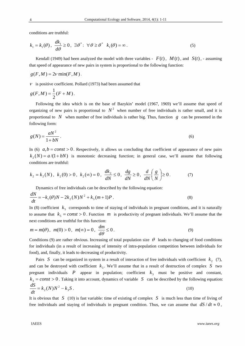
Graphically all possible transitions of individuals in population are presented on Fig. 1. Note, that such
kind of interactions is observed for various species, and, in particular, for earthworm (Lumbricina), for snails
Helix pomatia and for other species. Such kind of interaction is normal for simultaneous (or synchronic)
hermaphrodites.
3 Some Properties of Model (12)
1. For non-negative and finite initial values of variables solutions of the system (12) are non-negative and
bounded.
2. Let
0)1()(2)(),( 52
211 PmkNNkNkPNF ,
0)()(2),( 452
22 PkPkNNkPNF .
(13)
From (5), (7), and (9) we obtain the following inequality:
0))((2)( 52
21
11
d
dmPkNNk
dN
d
d
dkNk
N
F.
It means that isocline of vertical inclines of system (12) 0),(1 PNF is a single-valued function with
respect to P . For isocline of horizontal inclines we have the following inequality:
0)( 445
2
d
dkPkk
P
F.
5
Computational Ecology and Software, 2014, 4(1): 1-11
IAEES www.iaees.org
Thus, isocline of horizontal inclines (13) is a single-valued function with respect to N . Conditions (5), (7),
(9) for coefficients jk , 5,...,1j , don’t allow determining of signs for expressions PF /1 and
NF /2 .
Fig. 1 All possible transformations of individuals in population. 1k and 4k are intensities of death rate. 2k is coefficient of forming of pair S . 3k is coefficient of destruction of pair S . 5k is a coefficient of staying of individual in pregnant state. m is number of new free individuals which are produced by one pregnant individual.
3. Previous properties of model (12) give us the following inequality:
021
P
F
N
F.
Thus, there are no limit cycles in phase space (Bendixon’ criteria; Andronov, Vitt, Khykin, 1959).
Consequently, within the framework of model (12) there are the regimes of asymptotic stabilization of
population size at any level only.
4. Origin )0,0( is stationary state of system (12). This system in sufficient small vicinity of origin can be
prersent6ed in following form:
PmkNkdt
dN)1)0(()0( 51 ,
PkPkdt
dP)0(45 .
Thus, characteristic values are negative: )0(11 k and )0(452 kk . Consequently, in all
situations origin is stable knot.
5. In a situation when we have a parametric model (model of Volterra type) we have the following main goal:
we have to present a structure of a space of model parameters and to point out dynamical regimes which
correspond to each determined part of space of parameters. When we have a non-parametric model (model of
Kolmogorov type like in current publication) we have other main goal: in a result of provided analysis we have
to present dynamical regimes which can be realized in model in principle, and their realization not in a
contradiction with considering restrictions on the types of functions in right-hand sides of equations. Below
we’ll consider some simplest dynamic regimes of model (12) – restrictions (8)-(11) and (14) don’t allow
presenting all possible dynamic regimes which can be observed within the framework of model.
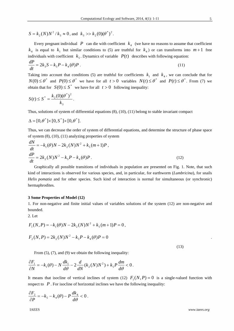
If algebraic system (13) has no solutions in positive part of phase plane, origin is global stable equilibrium.
Population eliminates for all non-negative finite initial values (Fig. 2).
6
Computational Ecology and Software, 2014, 4(1): 1-11
IAEES www.iaees.org
Fig. 2 Regime of population elimination for all initial values of variables. 01 F and 02 F are the main isoclines of vertical and horizontal inclines of model trajectories respectively.
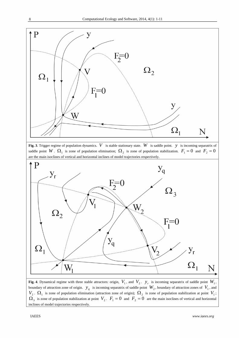
If algebraic system (13) has two solutions in positive part of phase plane the trigger regime is realized for
population: there are two stable attractors on phase plane (Fig. 3). Incoming separatrix y of saddle point W
divides zones of attraction of origin and stable equilibrium V . If initial sizes of variables are rather small
(within the limits of zone of elimination 1 ; Fig. 3) population eliminates asymptotically. If initial values
belong to another zone (zone of stabilization 2 ) sizes of both variables stabilize asymptotically at unique
level.
In general case within the limits of model (12) dynamic regimes with several stationary states in positive
part of phase plane can be realized (see, for example, Fig. 4). When difference between total numbers of sizes
which correspond to various stable stationary states are rather big, it can be considered as direct analog of the
regime of fixed outbreak (Isaev et al., 1978, 1980; Isaev et al., 1984, 2001). Thus, we can conclude that big
difference between pregnant individuals and free individuals can be a reason for population elimination or a
reason for transmission of system from one stable level to another one (see Fig. 4). Such kind of changing of
population size can be interpreted as unstable behavior of population within the limits of zone of population
stability (Isaev et al., 1978, 1980; Isaev et al., 1984, 2001).
7
Computational Ecology and Software, 2014, 4(1): 1-11
IAEES www.iaees.org
Fig. 3. Trigger regime of population dynamics. V is stable stationary state. W is saddle point. y is incoming separatrix of
saddle point W . 1 is zone of population elimination; 2 is zone of population stabilization. 01 F and 02 F
are the main isoclines of vertical and horizontal inclines of model trajectories respectively.
Fig. 4. Dynamical regime with three stable attractors: origin, 1V , and 2V . ry is incoming separatrix of saddle point 1W ,
boundary of attraction zone of origin. qy is incoming separatrix of saddle point 2W , boundary of attraction zones of 1V , and
2V . 1 is zone of population elimination (attraction zone of origin); 2 is zone of population stabilization at point 1V ;
3 is zone of population stabilization at point 2V . 01 F and 02 F are the main isoclines of vertical and horizontal
inclines of model trajectories respectively.
8
Computational Ecology and Software, 2014, 4(1): 1-11
IAEES www.iaees.org
4 Conclusion
Analysis of model of hermaphrodite population dynamics shows that in general case dynamic regimes with
several non-trivial stationary states can be observed for the system. It means that changing of sizes of free and
pregnant individuals (for example, under the influence of various management methods) can lead as to
transaction of system from one stable level to another one, as to extinction of population. Existence of several
stable levels in positive part of phase plane can be a reason of unstable behavior of system in zone of
population stability (Isaev et al., 1978, 1980).
References
Alexeev VI, Ginzburg LR. 1969. About a population size regulation by biological methods. Journal of General
Biology, 30(5): 616-620
Alvarez OA, Jager T, Colao BN, Kammenga JE. 2006. Temporal dynamics of effect concentrations.
Environmental Science and Technology, 40: 2478-2484
Andronov AA., Vitt AA., Khykin SE. 1959. Theory of Oscillations. Fizmatgiz, Moscow, Russia
Armsworth PR. 2001. Effects of fishing on a protogynous hermaphrodite. Canadian Journal of Fisheries and
Aquatic Sciences, 58: 568-578
Barker GM. 2002. Mollusks as Crop Pests. CABI, India
Batlutskaya IV, Makanina OA, Prokhorova EA. 2010. The study of dynamics of sexual structure of red-soldier
bugs’ population (Pyrrhocoris arterus L.) from different biotopes. Bulletin SamSU, 6(80): 173-178
Bazykin AD. 1967. About comparison of effectiveness of some methods of population density regulation.
Journal of General Biology, 28(4): 463-466
Bazykin AD. 1969. Model of species dynamics and problem of co-existence of nearest species. Journal of
General Biology, 30(3): 259-264
Bazykin AD. 1985. Mathematical Biophysics of Interacting Populations. Nauka, Moscow, Russia
Bolshakov VN, Kubantsev BS. 1984. Sex structure of mammal populations and its dynamics. Nauka, Moscow,
Russia
Brezhnev AI, Ginzburg LR. 1974. Toward an estimation of norm of sterile insects input. Journal of General
Biology, 35(6): 911-916
Brezhnev AI, Ginzburg LR, Poluektov RA, Shvitov IA. 1975. Mathematical models of biological communities
and problems of management. In: Mathematical Modeling in Biology (Molchanov AM, ed). 92-112,
Nauka, Moscow, Russia
Castillo-Chaves C, Yakubu AA., Thieme HR., Martcheva M. 2002. Nonlinear mating models for populations
with discrete generation. In: Mathematical Approaches for Emerging and Reemerging Infectious Diseases:
An Introduction (Castillo-Chavez C, Blower S, Van den Driessche P, et al., eds). 251-268, Springer, New
York, USA
Charnov EL, Bull JJ, Maynard SJ. 1976. Why be an hermaphrodite? Nature 263: 125-126
Cheptou PO. 2004. Allee effect and self-fertilization in hermaphrodites: reproductive assurance in
demographically stable populations. Evolution, 58(12): 2613-2621
Civeyrel L, Simberloff D. 1996. A tale of two snails: is the cure worse than the disease? Biodiversity and
Conservation, 5(10): 1231-1252
Costello WG, Taylor HM. 1975. Mathematical Models of the Sterile Male Technique of Insect Control.
Lecture Notes in Biomathematics 5. 318-359, Springer Berlin, Heidelberg, German
Frisman EY, Revutskaya OL, Neverova GP. 2010a. Complex dynamics of the population with age and sex
9
Computational Ecology and Software, 2014, 4(1): 1-11
IAEES www.iaees.org
structure. Dokladi of Russian Academy of Sciences, 431(6): 844-848
Frisman EY, Revutskaya OL, Neverova GP. 2010b. Modeling of the dynamics of limited population with age
and sex structure. Mathematical Modeling, 22(11): 65-78
Frisman EYa, Neverova GP, Revutskaya OL. 2011. Complex dynamics of the population with a simple age
structure. Ecological Modelling, 222: 1943-1950
Geodakjan VA. 1965. Role of sexes in transmission and transformation of a genetic information. Problems of
Information Transmission, 1(1): 105-112
Geodakjan VA. 1981. Sex dimorphism and “father’s effect” Journal of General Biology, 42(5): 657-668
Geodakjan VA. 1991. Evolution theory of sex. Nature, 8: 60-69
Gimelfarb AA, Ginzburg LR, Poluektov RA, et al. 1974. Dynamical Theory of Biological Populations. Nauka
Moscow, Russia
Ginzburg LR. 1969. Dynamics of two interacting populations of predator-prey system when sex structures are
taken into account. In: Publications in Agronomic Physics (Poluektov RA, ed). 6: 139-143,
Gidrometeoizdat, Leningrad, Russia
Ginzburg LR, Yuzefovich GI. 1968. About a sexes dynamics in bisexual population. Genetics, 4(12): 116-119
Goodman LA. 1953. Population Growth of the Sexes. Biometrics, 9: 212-225
Goodman LA. 1967. On the age-sex composition of the population that would result from given fertility and
mortality conditions. Demography, 4: 423-441
Grechanii GV, Pogodaeva MV. 1996. Changing of sex structure of Taufliege population at size dynamics.
Genetics, 32(10): 1349-1353
Hadeler K. 1992. Periodic solutions of homogeneous equations. Journal of Differential Equations, 95: 183-202
Hadeler K. 1993. Pair formation with maturation period. Journal of Mathematical Biology, 32: 1-15
Hadeler K, Ngoma K. 1990. Homogeneous models for sexually transmitted diseases. Rocky Moutain Journal
of Mathematics, 20: 635-649.
Hadeler K, Waldstatter R, Worz-Busekros A. 1988. Models for pair formation in bisexual populations. Journal
of Mathematical Biology, 26: 635-649
Harder LD, Richards SA, Routley MB. 2007. Effects of reproductive compensation, gamete discounting and
reproductive assurance on mating-system diversity in Hermaphrodites. Evolution, 62(1): 157-172
Iannelli M., Martcheva M., Milner FA. 2005. Gender-structured Population Modelling: Mathematical Models,
Numerics, and Simulations. SIAM, Philadelphia, USA
Isaev AS, Nedorezov LV, Khlebopros RG. 1978. Influence of Escape Effect on Predator – Prey System
Dynamics. Computing Center SB AS USSR, Krasnoyarsk, Russia
Isaev AS, Nedorezov LV, Khlebopros RG. 1980. Qualitative Analysis of the Phenomenological Model of the
Forest Insect Number Dynamics. Pest Management Network 9. 1-44, IIASA, Austria
Isaev AS, Khlebopros RG, Nedorezov LV, et al. 1984. Forest Insect Population Dynamics. Nauka,
Novosibirsk, Russia
Isaev AS, Khlebopros RG, Nedorezov LV, et al. 2001. Population Dynamics of Forest Insects. Nauka,
Moscow, Russia
Kebir A, Ben Miled S, Hbid ML, Bravo de la Parra R. 2010. Effects of density dependent sex allocation on the
dynamics of a simultaneous hermaphroditic population: Modelling and analysis. Journal of Theoretical
Biology, 263(4): 521-529
Kendall DG. 1949. Stochastic processes and population growth. Journal of the Royal Statistical Society: Series
B, 11: 230-264
10

Computational Ecology and Software, 2014, 4(1): 1-11
IAEES www.iaees.org
Kiester AR, Nagylaki T, Shaffer B. 1981. Population dynamics of species with gynogenetic sibling species.
Theoretical Population Biology, 19: 358-369
Maynard SJ. 1978. The Evolution of Sex. Cambridge University Press, UK
Nedorezov LV. 1978. About some self-educated population models. In: Educated Algorithms in Systems of
Management and Analysis of Information (Medvedev AV, ed). 69-83, Nauka, Novosibirsk, Russia
Nedorezov LV. 1979. Influence of Inherent Structures of Populations on the Dynamics of Phytophagous Mass
Propagations. Mathematical Models of Bisexual Population Dynamics. Preprint of the Institute of Forest
and Wood AS of the USSR, Krasnoyarsk, Russia
Nedorezov LV. 1983. The Influence of the sterile individuals onto the population dynamics. Izvestia SB AS
USSR, 10: 119-122
Nedorezov LV. 1986. Modeling of Forest Insect Outbreaks. Nauka, Novosibirsk, Russia
Nedorezov LV, Utyupin YuV. 2003. Discrete-continuous model of bisexual population dynamics. Siberian
Mathematical Journal, 44(3): 650-659
Nedorezov LV, Utyupin YuV. 2011. Continuous-Discrete Models of Population Dynamics: An Analytical
Overview. Ser. Ecology. Vip. 95. State Public Scientific-Technical Library, Novosibirsk, Russia
Pertsev NV. 2000. About a model of population size dynamics with forming and destruction of family’s pairs.
Mathematical Structures and Modeling, 6: 101-106
Preece T, Mao Y. 2009. Sustainability of dioecious and hermaphrodite populations on a lattice. Journal of
Theoretical Biology, 261(2): 336-340
Pollard JH. 1973. Mathematical Models for the Growth of Human Populations. Cambridge University Press,
UK
Stewart AD, Phillips PC. 2002. Selection and maintenance of androdioecy in Caenorhabditis elegans.
Genetics, 160: 975-982
Thome RCA, Hyun Mo Yang, Esteva L. 2010. Optimal control of Aedes aegypti mosquitoes by the sterile
insect technique and insecticide. Mathematical Biosciences, 223: 12-23
Yellin J, Samuelson P. 1974. A dynamical model for human population. Proceedings of the National Academy
of Sciences of USA, 71: 2813-2817
Yellin J, Samuelson P. 1977. Comparison of linear and nonlinear models for human population dynamics.
Theoretical Population Biology, 11: 105-126
11
Computational Ecology and Software, 2014, 4(1): 12-21
IAEES www.iaees.org
Article
Temporal mortality-colonization dynamic can influence the
coexistence and persistence patterns of cooperators and defectors in
an evolutionary game model
YouHua Chen1, XueKe Lu2, YouFang Chen3 1Department of Renewable Resources, University of Alberta, Edmonton, T6G 2H1, Canada 2Department of Electronic Engineering and Computer Science, Queen Mary University of London, E1 4NS, UK 3School of Software, Harbin Normal University, Heilongjiang Province, China
E-mail: [email protected]
Received 28 October 2013; Accepted 2 December 2013; Published online 1 March 2014
Abstract
In the present report, the coexistence and persistence time patterns of Prisoners’ Dilemma game players were
explored in 2D spatial grid systems by considering the impacts of the mortality-colonization temporal dynamic
specifically. Our results showed that the waiting time for triggering a colonization event could remarkably
influence and change the extinction patterns of both cooperators and defectors. Interestingly, a relatively high
frequency of stochastic colonization events could promote the persistence of defectors but not cooperators. In
contrast, a low frequency of stochastic- or constant-time colonization events could facilitate the persistence of
cooperators but not defectors. However, a long waiting time would be detrimental to the survival of both game
players and drives them to go extinction in faster rates. At last, it was found that colonization strength played a
relatively weak role on influencing the coexistence scenarios of both game players, but should be kept small if
the coexistence of game players is needed to maintain. In conclusion, our study provides evidence showing
that the temporal trade-off of mortality and colonization activities would influence the evolution of PD game
and the persistence of cooperators and defectors.
Keywords species coexistence; game theory; colonization-extinction dynamics; individual-based modeling.
1 Introduction
The classical Prisoner’s Dilemma (PD) game has been broadly studied in evolutionary biology (Hui and
McGeoch, 2007; Zhang and Hui, 2011; Zhang et al., 2005; Nowak and May, 1993, 1992; Zhang, 2012).
Spatial version of Prisoner’s Dilemma could allow the emergence of complex defense-cooperation dynamic
patterns and make the cooperation become more possible (Langer et al., 2008; Zhang et al., 2005).
Computational Ecology and Software ISSN 2220721X URL: http://www.iaees.org/publications/journals/ces/onlineversion.asp RSS: http://www.iaees.org/publications/journals/ces/rss.xml Email: [email protected] EditorinChief: WenJun Zhang Publisher: International Academy of Ecology and Environmental Sciences
Computational Ecology and Software, 2014, 4(1): 12-21
IAEES www.iaees.org
In a previous study, the evolution of cooperation under habitat destruction has been well quantified (Zhang
et al., 2005). One important part of the model used by the previous work (Zhang et al., 2005) is to model the
dynamic between mortality and colonization. However, the trade-off between the occurrence frequency of
colonization and mortality events and the relevant impacts on the coexistence and survival of both game
players have not been extensively evaluated yet. Because in the previous study (Zhang et al., 2005),
colonization and mortality events are allowed to happen at each simulation time step. A detailed study on the
trade-off between colonization and mortality occurrence frequency would allow ones to better understant the
real-time habitat degeneration and isolation processes on influencing the coexistence patterns of cooperators
and defectors.
In the present report, We quantify the condition of coexistence of both defectors and cooperators by
varying the occurrence frequency of colonization and mortality events. In specific, We fix the mortality
frequency during the simulation (allowed to occur one time per one time step), and evaluate the influence of
waiting time of triggering a colonization event on the persistence of cooperators and defectors.
As a summary, the central objective of the present study is to reveal the impacts of the temporal trade-off
of the occurrence frequency of colonization and mortality events on the persistence time of PD game players.
2 Materials and Methods
The payoff matrix of a typical evolutionary PD game is defined as (Zhang et al., 2005),
C D
C
D
(1)
where >0 and >0. C represents the cooperator, while D represents the defector.
Assuming that each patch is only allowed to inhabit one individual, the ip score for the individual in the
patch i, taking into account of the rewards during the evolutionary game interaction, is defined as follows
(Zhang et al., 2005),
( 1) ( 1)( ) ( )
2 2i i i i
i i i ii C D C D
x x x xp f f f f (2)
Here we adopt the same notation used in the previous study (Hui et al., 2005). Where ix =1 if patch We is
occupied by a cooperator; ix =-1 if the patch is occupied by a defector; and ix =0 if it is empty. iCf is the
fraction of cooperators in the two neighboring patches of the patch We and iDf is the fraction of defectors.
Clearly,iCf +
iDf 1.
Degeneration of habitat quality is thought to be related to mortality rate, while patch isolation is related to
colonization rate of species (Zhang et al., 2005). As such, as mentioned above, the trade-off between mortality
and colonization frequency actually reflects the dynamic of habitat degeneration and isolation on the
persistence of both game players.
The mortality rate of individuals for taking into account of the degeneration of habitat quality is defined as
(Zhang et al., 2005),
exp( )( )
1 exp( )i
ii
pM p m
p
(3)
and the colonization rate of individuals is (Zhang et al., 2005),
13
Computational Ecology and Software, 2014, 4(1): 12-21
IAEES www.iaees.org
1( )
1 exp( )ii
C p cup
(4)
Here, m and c are regarded to be related to habitat degeneration and isolation respectively, being in the range
of [0, 1]. Higher values of m and/or c indicates higher degrees of degeneration and/or isolation of the habitat.
Hereafter, We call m and c as mortality and colonization coefficients (or strengths) respectively.
For modeling the temporal impact of trade-off between mortality and colonization events, We define and
use the waiting time of triggering a colonization event. In detail, a mortality event is assumed to happen for
each time step, while a colonization event could happen only when the next time for triggering it satisfying the
waiting time (WT) setting.
Two strategies are used to configure the waiting time setting for triggering a colonization event during the
simulation. The first one is to assume the waiting time of a colonization (WT) event is deterministic and
constant, which is fixed to be an integral. As such, the colonization or mortality events could happen at the
time steps when they are the integral multiples of the waiting time value. For example, if a waiting time for a
colonization event is set to WT=12, then the colonization events could happen in the time steps 12, 24, 36 and
so on. As such, WT measures how many time steps are required to trigger a colonization event. When the
simulation has a total time step of 100, the overall colonization event number should 100/12 8.
The second strategy is to assume the waiting time of a colonization event being stochastic. The stochastic
waiting time is modeled by an acceptance rate (still use WT to indicate the acceptance rate, being less than 1
and larger than 0) and a variate randomly drawn from the uniform distribution [0,1]. Different from the
constant WT cases, for stochastic WT, for each time step, a colonization event could be allowed to happen
only when the randomly drawn variate is smaller than the acceptance rate WT. Consequently, for stochastic
WT cases, an acceptance rate WT indicates how many colonization events could happen during the simulation.
For example, if WT=0.5, and the simulation time is 100 as a total, then the overall colonization event number
for the simulation is 1000.5=50.
Finally, it is worth noting that, whether stochastic or constant strategies are applied, WT=1 always implies
a perfect synchrony between colonization and mortality events because both are allowed to happen at each
time step.
Based on the above definitions, for each time step, a mortality event has to happen, for which an individual
has the probability of ( )iM p to die and the patch becomes vacant again. In contrast for each time step, the
colonization of the vacant sites could be allowed only when the WT setting for a colonization event is satisfied.
When a colonization event can be allowed to happen, the vacant patch will be colonized by an offspring of
another individual from the neighboring patches (four neighboring cells are used in the present study: up, low,
left and right). Whether the offspring is a cooperator or defector is determined by following probabilities,
( 1)1( )
2 2i
j ji j
j S
x xPC C p
(5)
And
( 1)1( )
2 2i
j ji j
j S
x xPD C p
(6)
where iPC and iPD represent the probability of an offspring of the cooperators and defectors from the
neighboring patches of patch We to colonize the vacant patch i. If iPC > iPD , then the patch is colonized by
a cooperator offspring; if iPC < iPD , the patch is colonized by a defector offspring.
14

Computational Ecology and Software, 2014, 4(1): 12-21
IAEES www.iaees.org
During the simulation, we use the occurrence frequency of species (fraction of grid cells occupied) as the
index to quantify the influence of varying colonization waiting time on the coexistence and survival of both
game players. In our simulation, a 2D square grid system with periodic boundary conditions is employed with
a size of 5050. For each simulation, 1000 time step is used.
3 Results
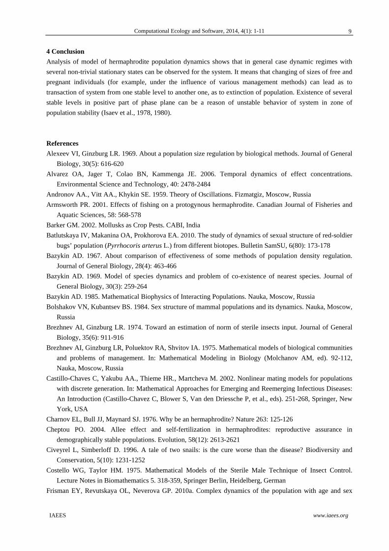
3.1 Coexistence of game players by varying mortality and colonization strengths
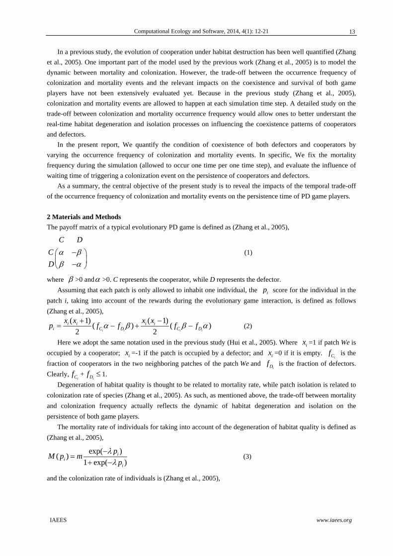
When evaluating the coexistence of both players as the function of mortality and colonization coefficients,
apparently, as indicated by the 3D surface plot (Fig. 1), lower mortality coefficient could allow the coexistence
and survival of both game players. Colonization coefficient c has little effect on the coexistence scenarios of
both game players. The coexistence of players is principally determined by mortality strength m.
3.2 Coexistence of game players by varying cooperation and defense rewards
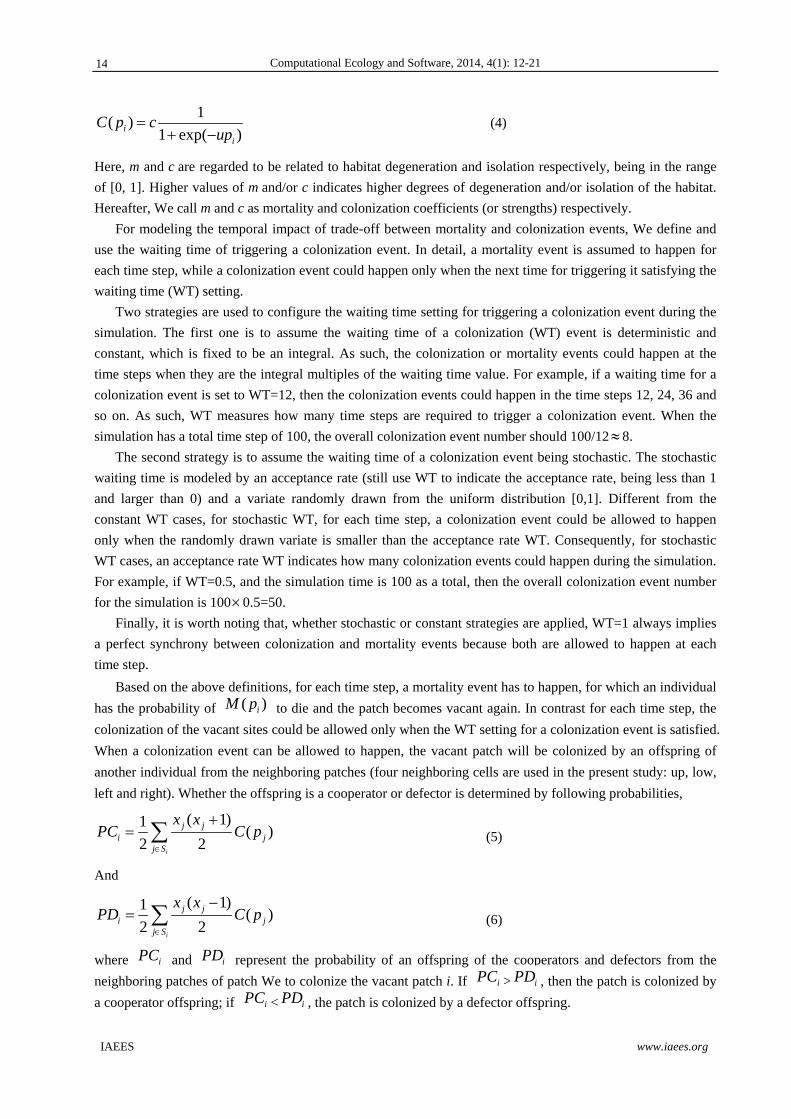
When evaluating the coexistence of both players as the function of cooperation and defense rewards, as
indicated by the 3D surface plot (Fig. 2), the linear combination between and reward could allow the
coexistence of both game players. Interestingly, for all the area with < and part of the region with >
could maintain the coexistence of both species. The latter could be applicable only when their difference is not
too large (Fig. 2). Otherwise, cooperators would dominate the community.
3.3 Coexistence of game players by varying defense reward and colonization strength
As showed in Fig. 3, high colonization coefficient c will lead to the dominance of defectors in the community,
while cooperators would die out. In contrast, when the colonization coefficient c is low, coexistence of both
game players are possible, regardless of the values of defense reward .
3.4 Coexistence of game players by varying waiting time and colonization strength
As showed in Fig. 4, varying either waiting time or colonization strength could not change the coexistence
pattern of cooperators and defectors. Both game players could coexist throughout the simulation, but
cooperators have higher population densities.
3.5 Coexistence of game players by varying waiting time and defense reward
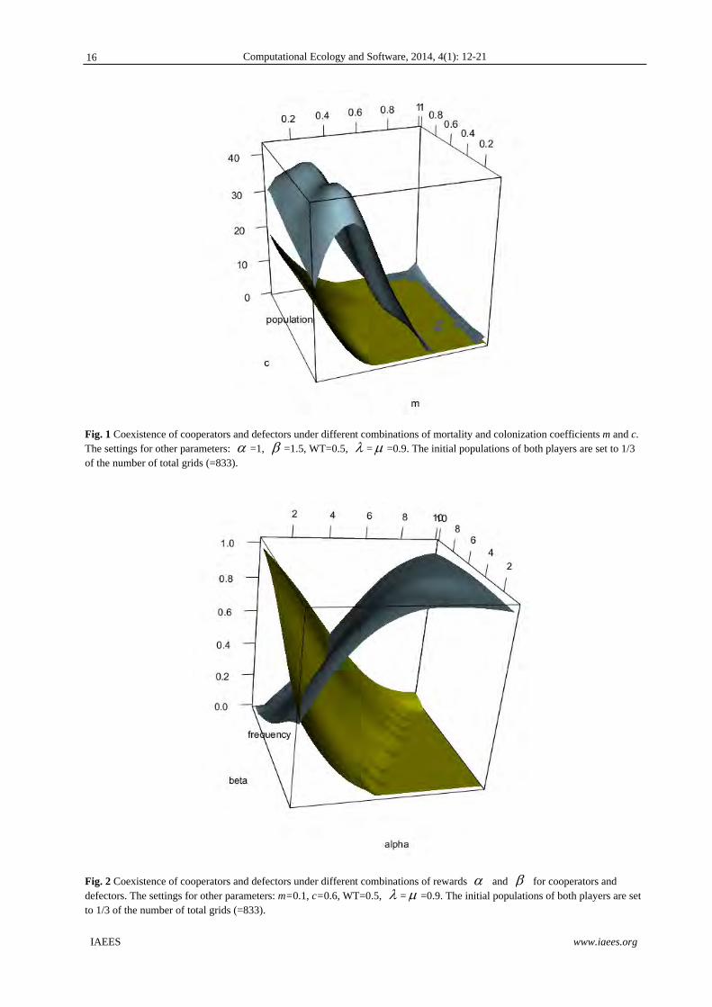
As showed in Fig. 5, only when waiting time is small and stochastic, the coexistence of both players is
possible. Otherwise, cooperators would dominate the community and defectors go extinct. Interestingly, the
population density of cooperators would become highest for the cases of defense reward >10 when WT is
around 13 (Fig. 5). Increasing or decreasing WT from the optimum would reduce the population of cooperators
in the community, regardless of the existence of defectors.
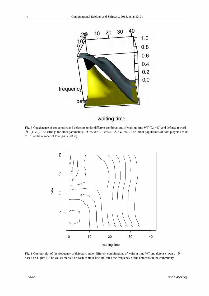
Another interesting thing is that the cooperators could not occupy all the vacant sites even when defectors
have been removed out of the community for most of parameter space (Fig. 6). An exception is found at the
bottom-left area which has the parameter space with small and long stochastic waiting time of triggering
colonization events (small WT approaches zero) (Fig. 6).
3.6 Persistence time of both cooperators and defectors for different waiting time situations of triggering
colonization events
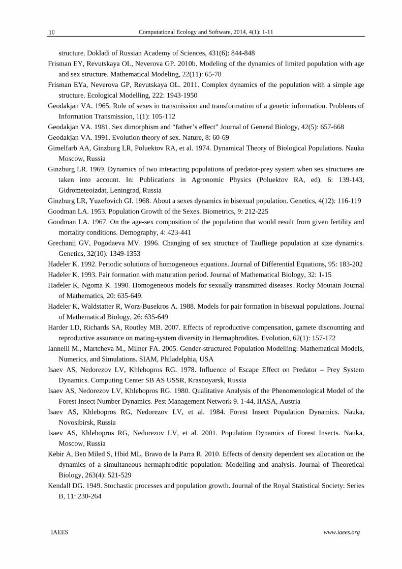
For the persistence time of defectors, a unimodal pattern was identified (Figs. 5 and 7). The longest persistence
time for the players could be found at WT=0.7 (indicating that for each time step, a 0.7 probability of
triggering a colonization event). The overall number of colonization events during a simulation with 800 time
step would be around 560. However, when WT becomes larger and the probability of triggering colonization
events becomes higher, the persistence time of the defectors in the community is decreased and they could not
survive until the end of the simulation.
15
Computational Ecology and Software, 2014, 4(1): 12-21
IAEES www.iaees.org
Fig. 1 Coexistence of cooperators and defectors under different combinations of mortality and colonization coefficients m and c. The settings for other parameters: =1, =1.5, WT=0.5, = =0.9. The initial populations of both players are set to 1/3 of the number of total grids (=833).
Fig. 2 Coexistence of cooperators and defectors under different combinations of rewards and for cooperators and defectors. The settings for other parameters: m=0.1, c=0.6, WT=0.5, = =0.9. The initial populations of both players are set to 1/3 of the number of total grids (=833).
16

Computational Ecology and Software, 2014, 4(1): 12-21
IAEES www.iaees.org
Fig. 3 Coexistence of cooperators and defectors under different combinations of defense reward and colonization coefficient c. The settings for other parameters: =1, m=0.1, WT=0.5, = =0.9. The initial populations of both players are set to 1/3 of the number of total grids (=833).
Fig. 4 Coexistence of cooperators and defectors under different combinations of waiting time WT and colonization coefficient c. The settings for other parameters: =1, =1.5, m=0.1, = =0.9. The initial populations of both players are set to 1/3 of the number of total grids (=833).
17
Computational Ecology and Software, 2014, 4(1): 12-21
IAEES www.iaees.org
Fig. 5 Coexistence of cooperators and defectors under different combinations of waiting time WT (0.1~40) and defense reward (1~20). The settings for other parameters: =5, m=0.1, c=0.6, = =0.9. The initial populations of both players are set to 1/3 of the number of total grids (=833).
Fig. 6 Contour plot of the frequency of defectors under different combinations of waiting time WT and defense reward based on Figure 5. The values marked on each contour line indicated the frequency of the defectors in the community.
waiting time
be
ta
0.1
0.2
0.3
0.3
0.4
0.4
0.5
0.5
0.6
0.6
0.7
0.8
0.9
1
0 10 20 30 40
51
01
52
0
18
Computational Ecology and Software, 2014, 4(1): 12-21
IAEES www.iaees.org
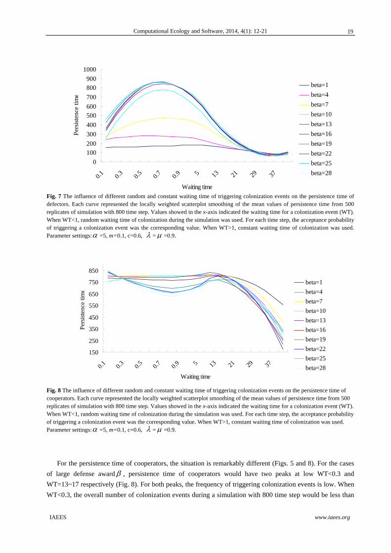
Fig. 7 The influence of different random and constant waiting time of triggering colonization events on the persistence time of defectors. Each curve represented the locally weighted scatterplot smoothing of the mean values of persistence time from 500 replicates of simulation with 800 time step. Values showed in the x-axis indicated the waiting time for a colonization event (WT). When WT<1, random waiting time of colonization during the simulation was used. For each time step, the acceptance probability of triggering a colonization event was the corresponding value. When WT>1, constant waiting time of colonization was used. Parameter settings: =5, m=0.1, c=0.6, = =0.9.
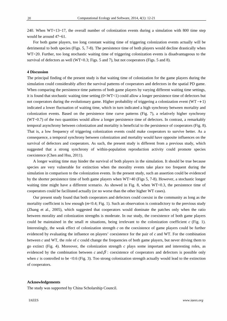
Fig. 8 The influence of different random and constant waiting time of triggering colonization events on the persistence time of cooperators. Each curve represented the locally weighted scatterplot smoothing of the mean values of persistence time from 500 replicates of simulation with 800 time step. Values showed in the x-axis indicated the waiting time for a colonization event (WT). When WT<1, random waiting time of colonization during the simulation was used. For each time step, the acceptance probability of triggering a colonization event was the corresponding value. When WT>1, constant waiting time of colonization was used. Parameter settings: =5, m=0.1, c=0.6, = =0.9.
For the persistence time of cooperators, the situation is remarkably different (Figs. 5 and 8). For the cases
of large defense award , persistence time of cooperators would have two peaks at low WT<0.3 and
WT=13~17 respectively (Fig. 8). For both peaks, the frequency of triggering colonization events is low. When
WT<0.3, the overall number of colonization events during a simulation with 800 time step would be less than
0
100200
300
400
500600
700
800900
1000
0.1 0.3 0.5 0.7 0.9 5 13 21 29 37
Waiting time
Per
sist
ence
tim
e
beta=1
beta=4
beta=7
beta=10
beta=13
beta=16
beta=19
beta=22
beta=25
beta=28
150
250
350
450
550
650
750
850
0.1 0.3 0.5 0.7 0.9 5 13 21 29 37
Waiting time
Per
sist
ence
tim
e
beta=1
beta=4
beta=7
beta=10
beta=13
beta=16
beta=19
beta=22
beta=25
beta=28
19
Computational Ecology and Software, 2014, 4(1): 12-21
IAEES www.iaees.org
240. When WT=13~17, the overall number of colonization events during a simulation with 800 time step
would be around 47~61.
For both game players, too long constant waiting time of triggering colonization events actually will be
detrimental to both species (Figs. 5, 7-8). The persistence time of both players would decline drastically when
WT>20. Further, too long stochastic waiting time of triggering colonization events is disadvantageous to the
survival of defectors as well (WT<0.3; Figs. 5 and 7), but not cooperators (Figs. 5 and 8).
4 Discussion
The principal finding of the present study is that waiting time of colonization for the game players during the
simulation could considerably affect the survival patterns of cooperators and defectors in the spatial PD game.
When comparing the persistence time patterns of both game players by varying different waiting time settings,
it is found that stochastic waiting time setting (0<WT<1) could allow a longer persistence time of defectors but
not cooperators during the evolutionary game. Higher probability of triggering a colonization event (WT 1)
indicated a lower fluctuation of waiting time, which in turn indicated a high synchrony between mortality and
colonization events. Based on the persistence time curve patterns (Fig. 7), a relatively higher synchrony
(WT~0.7) of the two quantities would allow a longer persistence time of defectors. In contrast, a remarkably
temporal asynchrony between colonization and mortality is beneficial to the persistence of cooperators (Fig. 8).
That is, a low frequency of triggering colonization events could make cooperators to survive better. As a
consequence, a temporal synchrony between colonization and mortality would have opposite influences on the
survival of defectors and cooperators. As such, the present study is different from a previous study, which
suggested that a strong synchrony of within-population reproduction activity could promote species
coexistence (Chen and Hsu, 2011).
A longer waiting time may hinder the survival of both players in the simulation. It should be true because
species are very vulnerable for extinction when the morality events take place too frequent during the
simulation in comparison to the colonization events. In the present study, such an assertion could be evidenced
by the shorter persistence time of both game players when WT>40 (Figs 5, 7-8). However, a stochastic longer
waiting time might have a different scenario. As showed in Fig. 8, when WT<0.3, the persistence time of
cooperators could be facilitated actually (or no worse than the other higher WT cases).
Our present study found that both cooperators and defectors could coexist in the community as long as the
mortality coefficient is low enough (m<0.4; Fig. 1). Such an observation is contradictory to the previous study
(Zhang et al., 2005), which suggested that cooperators would dominate the patches only when the ratio
between morality and colonization strengths is moderate. In our study, the coexistence of both game players
could be maintained in the small m situations, being irrelevant to the colonization coefficient c (Fig. 1).
Interestingly, the weak effect of colonization strength c on the coexistence of game players could be further
evidenced by evaluating the influence on players’ coexistence for the pair of c and WT. For the combination
between c and WT, the role of c could change the frequencies of both game players, but never driving them to
go extinct (Fig. 4). Moreover, the colonization strength c plays some important and interesting roles, as
evidenced by the combination between c and : coexistence of cooperators and defectors is possible only
when c is controlled to be <0.6 (Fig. 3). Too strong colonization strength actually would lead to the extinction
of cooperators.
Acknowledgements
The study was supported by China Scholarship Council.
20

Computational Ecology and Software, 2014, 4(1): 12-21
IAEES www.iaees.org
References
Chen Y, Hsu S. 2011. Synchronized reproduction promotes species coexistence through reproductive
facilitation. Journal of Theoretical Biology, 274: 136-144
Hui C, McGeoch M. 2007. Spatial patterns of prisoner’s dilemma game in metapopulations. Bulletin of
Mathematical Biology, 69: 659-676
Hui C, Zhang F, Han X, Li Z. 2005. Cooperation evolution and self-regulation dynamics in metapopulation:
stage-equilibrium hypothesis. Ecological Modelling, 184: 397-412
Langer P, Nowak M a, Hauert C. 2008. Spatial invasion of cooperation. Journal of Theoretical Biology, 250:
634-641
Nowak M, May R. 1992. Evolutionary games and spatial chaos. Nature, 359: 826-829
Nowak M, May R. 1993. The spatial dimemmas of evolution. International Journal of Bifurcation and Chaos,
3: 35-78
Zhang F, Hui C. 2011. Eco-evolutionary feedback and the invasion of cooperation in prisoner’s dilemma
games. PLoS One, 6: e27523
Zhang F, Hui C, Han X, Li Z. 2005. Evolution of cooperation in patchy habitat under patch decay and isolation
Ecological Research, 20: 461-469
Zhang WJ. 2012. Computational Ecology: Graphs, Networks and Agent-based Modeling. World Scientific,
Singapore
21
Computational Ecology and Software, 2014, 4(1): 22-34
IAEES www.iaees.org
Article
An online calculator for spatial data and its applications
Kalle Remm, Tiiu Kelviste Institute of Ecology and Earth Sciences, University of Tartu. 46 Vanemuise St., 51014 Tartu, Estonia
E-mail: [email protected]
Received 6 December 2013; Accepted 10 January 2014; Published online 1 March 2014
Abstract
An online calculator (http://digiarhiiv.ut.ee/kalkulaator/) for statistical analysis of spatial data is introduced.
The calculator is applicable in a wide range of spatial research and for courses involving spatial data analysis.
The present version of the calculator contains 35 web pages for statistical functions with several options and
settings. The input data for most functions are pure Cartesian coordinates and variable values, which should be
copied to the input cell on the page of a particular spatial operation. The source code for the computational part
of all functions is freely available in C# programming language. Examples are given for thinning spatially
dense observation points to a predefined minimum distance, for calculating spatial autocorrelations, for
creating habitat suitability maps and for generalising movement data into spatio-temporal clusters.
Keywords spatial statistics; online tool; habitat suitability; autocorrelation; spatio-temporal clustering.
1 Introduction
Statistical problems in ecology, earth and environmental sciences, human geography, and other fields of
science and technology are often related to location or distance between observations. Spatial statistics deals
with functions that involve location in one way or another. For example, calculating mean precipitation level at
weather stations is not spatial statistics, as the location of stations is not involved in the summarising. Finding
out how the difference in precipitation values is related to the distance between stations is spatial analysis since
location is directly involved.
Scientific studies can be divided into descriptive (exploratory) and inferential (confirmatory) approach.
Exploratory spatial statistics deals with finding generalised values, relationships, spatial patterns, spatial
clustering and segmentation (Zhang, 2010). The first goal of inferential spatial analysis is usually to prove the
non-randomness of the pattern, followed by attempts to find possible reasons and to model the processes which
created the non-randomness.
Spatial statistical functions are included into major commercial GIS (Geographical Information Science)
software packages. Tools for spatial statistical analysis in freeware packages like QGIS are much more limited.
Computational Ecology and Software ISSN 2220721X URL: http://www.iaees.org/publications/journals/ces/onlineversion.asp RSS: http://www.iaees.org/publications/journals/ces/rss.xml Email: [email protected] EditorinChief: WenJun Zhang Publisher: International Academy of Ecology and Environmental Sciences

Computational Ecology and Software, 2014, 4(1): 22-34
IAEES www.iaees.org
There are ample online calculators for mathematical functions and ordinary statistical tests (see, e.g.
http://www.martindalecenter.com/Calculators2.html), but an online calculator for spatial analysis is hard to
find. Existing online calculators for spatial data mostly transform geodetic coordinates only.
The goal of this publication is to introduce the spatial data calculator at http://digiarhiiv.ut.ee/kalkulaator/
that is applicable in a wide range of spatial research and supports several courses on data management and
programming at the University of Tartu. The idea was formed, the original user interface designed and the
coding and testing project mainly developed by the first author. From the technological side, the calculator was
developed as Microsoft ASP.NET project, functions written in the C# programming language. The calculator
was created primarily for teaching and learning purposes, although has already been used in research (Kotta et
al., 2013). Computations for the following examples are made using the online calculator.
2 Main Characteristics of the Calculator
The calculator currently involves a home page and 35 web pages for statistical functions; 28 of these are
directly for spatial analysis. Most pages have several options to set the initial parameters for calculations. The
calculator does not demand any client-side installation other than a web browser. Input data and the parameters
set by the user are transferred to the server, which responds with computation results to the client's browser.
The calculator has no extra demands on the memory or processing unit of the client's device except for data
transfer and browsing ability. The amount of input data and the choice of functions are restricted, as online
applications are expected corresponding within a reasonable period of time. The restrictions depend on
function. Generally, for larger data sets and more complicated tasks, special GIS and/or statistical software
should be used instead.
Data input to most functions must be pure Cartesian coordinates and variable values. The input cell of a
web page in the calculator can be filled with example data by clicking the "Example data" button.
The measurement units of output distances and input parameters are the same as for coordinates, e.g. if the
coordinates are given in metres, then distance intervals and search radii must also be in metres. The decimal
separator must be a point, and the column separator a space, tab or semicolon. Empty cells are not allowed –
these should be filled or removed during data mounting. It is easy to prepare the input matrix as a spreadsheet
(Excel, Access) and to copy the values without column headers to the input cell of the online calculator. The
introductory text at every statistical function, as well as example data, indicate the necessary format of input
data. The point data can be in one data set or alternatively as separate samples of source locations and
destination points. In the last case, distances are measured only between two types of points. The web pages of
the calculator functions also include buttons for viewing a scatter plot of input data in a pop-up window, a
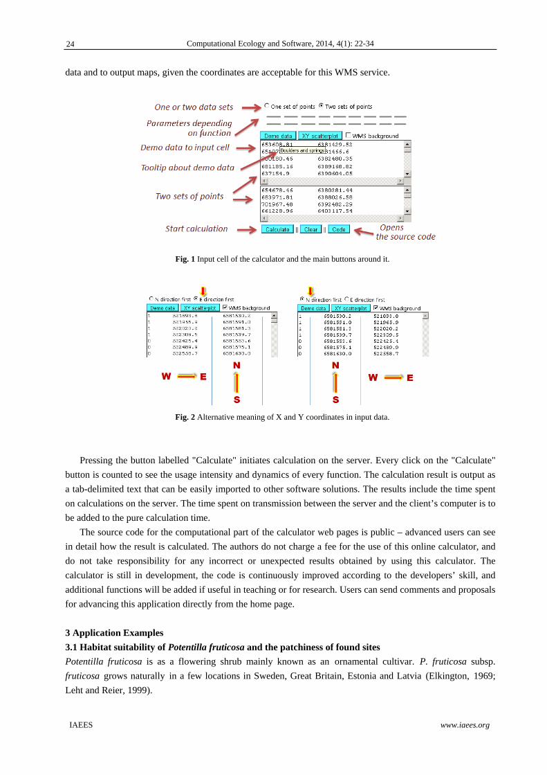
button that initiates calculation, and a button that opens the source code window (Fig. 1).
The meaning of X and Y coordinates as input columns can be switched with regard to which is the west-
east direction and which is south-north (Fig. 2). The X axis of example data in the calculator is always directed
to the east. For the European cartographic system, where the first coordinate axis is directed to the north, the
north direction must be set to the first position (select option "N direction first").
Suitability surface as an Idrisi unpacked headerless rst format raster can be added in several functions. It
enables the user, for example, to delimit the location of generated random points, and to define an irregularly
shaped, uneven and/or patchy study surface.
The location of input data points can be visualised in a pop-up window as an XY scatterplot or a bubble
chart, if the data points have values. Area borders set by the user determine the extent of the scatterplot, the
borders of the suitability surface (if used), and delimit random locations for the null model. A map background
from the Web Map Service (WMS) server of the Estonian Land Board can be added to scatterplots of source
23
Computational Ecology and Software, 2014, 4(1): 22-34
IAEES www.iaees.org
data and to output maps, given the coordinates are acceptable for this WMS service.
Fig. 1 Input cell of the calculator and the main buttons around it.
Fig. 2 Alternative meaning of X and Y coordinates in input data.
Pressing the button labelled "Calculate" initiates calculation on the server. Every click on the "Calculate"
button is counted to see the usage intensity and dynamics of every function. The calculation result is output as
a tab-delimited text that can be easily imported to other software solutions. The results include the time spent
on calculations on the server. The time spent on transmission between the server and the client’s computer is to
be added to the pure calculation time.
The source code for the computational part of the calculator web pages is public – advanced users can see
in detail how the result is calculated. The authors do not charge a fee for the use of this online calculator, and
do not take responsibility for any incorrect or unexpected results obtained by using this calculator. The
calculator is still in development, the code is continuously improved according to the developers’ skill, and
additional functions will be added if useful in teaching or for research. Users can send comments and proposals
for advancing this application directly from the home page.
3 Application Examples
3.1 Habitat suitability of Potentilla fruticosa and the patchiness of found sites
Potentilla fruticosa is as a flowering shrub mainly known as an ornamental cultivar. P. fruticosa subsp.
fruticosa grows naturally in a few locations in Sweden, Great Britain, Estonia and Latvia (Elkington, 1969;
Leht and Reier, 1999).
24
Computational Ecology and Software, 2014, 4(1): 22-34
IAEES www.iaees.org
For the following example, we used points on GPS-recorded field observation tracks and found locations
of this species from a study area of 10 km × 10 km square (sheet 6382 of the Estonian 1: 20 000 base map) in
the middle of the natural distribution area of P. fruticosa in north-west Estonia. Coordinates of observation
tracks and P. fruticosa observation locations were recorded using a Garmin Vista HC+ GPS recorder during
field trips on foot by the first author in summers 2008–2013. The initial data contained 12,299 track points and
1469 observation locations. Firstly, all automatically recorded track points closer than 50 m from active
observation points were removed using the online calculator’s thinning function. Then, both recorded track
points and observation locations were thinned to have at least 50 m between each accepted site. The thinned
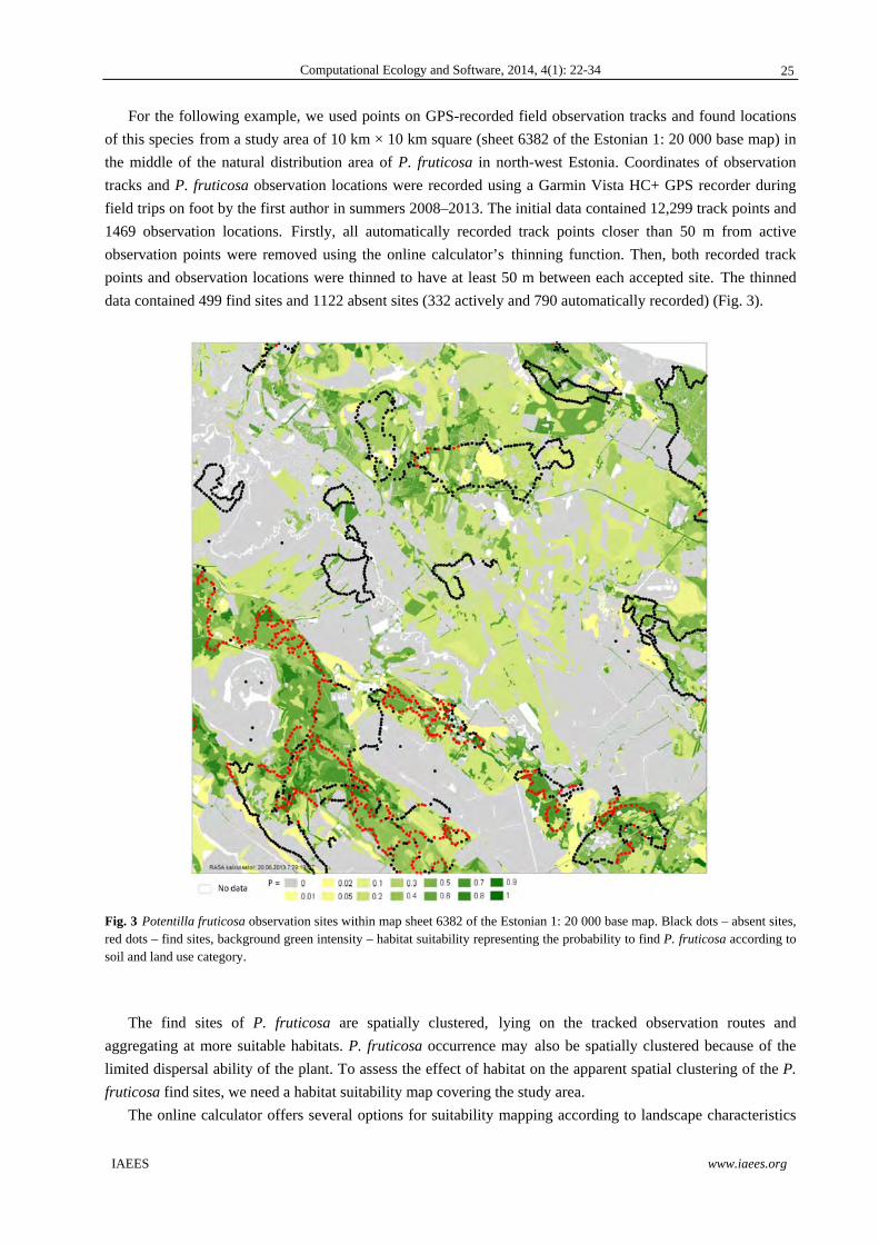
data contained 499 find sites and 1122 absent sites (332 actively and 790 automatically recorded) (Fig. 3).
Fig. 3 Potentilla fruticosa observation sites within map sheet 6382 of the Estonian 1: 20 000 base map. Black dots – absent sites, red dots – find sites, background green intensity – habitat suitability representing the probability to find P. fruticosa according to soil and land use category.
The find sites of P. fruticosa are spatially clustered, lying on the tracked observation routes and
aggregating at more suitable habitats. P. fruticosa occurrence may also be spatially clustered because of the
limited dispersal ability of the plant. To assess the effect of habitat on the apparent spatial clustering of the P.
fruticosa find sites, we need a habitat suitability map covering the study area.
The online calculator offers several options for suitability mapping according to landscape characteristics
25
Computational Ecology and Software, 2014, 4(1): 22-34
IAEES www.iaees.org
by calculating: 1) combinations of presence and absence frequency; 2) probability of occurrence, and 3)
expected presence or absence according to similarity of sites using either the k nearest neighbours (kNN), d
nearest neighbours (dNN) or sumsim algorithm. For the kNN algorithm, the number of the most similar
exemplars included has to be fixed; dNN algorithm sets a limit on the acceptable similarity level; the sumsim
algorithm, which is applied in the Constud software system (Remm and Kelviste, 2011; Remm and Remm,
2008), needs the sum of similarity of the most similar accepted exemplars to be given.
For this study, habitat suitability of P. fruticosa was calculated using probability mapping within a map
sheet. The resulting map indicates a higher probability to find the plant in alvar grasslands, where the land
cover category is either bush land or so-called other (unmanaged) open land, and the favourite soil categories
are Gleisoil, Endogleyic Luvisol, and Rendzic Leptosol. The bushes in these alvar grasslands are mainly
junipers.
The second part of this example is analysing the spatial pattern of P. fruticosa find sites. A spatial pattern
of points: its clustering, regularity or randomness can be described in a generalised form using several formal
statistics presented in the online calculator: the nearest neighbour distances, distribution of all distances
between points, the mean squared distance, K(t), L(t)−t, O(r), G(r), F(r), and J(r) functions. Clustering of P.
fruticosa find sites relative to total area, to estimated habitat suitability, to observation sites, and to suitability
weighted observation sites according to K(t), L(t)−t and O(r) statistics with 95% confidence envelope,
calculated using the online calculator, is presented here as an example.
The K(t) statistic was introduced by B.D. Ripley (Ripley, 1976, 1977, 1981) as the mean number of
neighbouring objects within radius t from a source point divided by the mean density of objects. Letters d and r
often stand for radius in the K(t) function instead of Ripley's original sign, t. In the following, r is preferred to
make the notation of radius uniform. The expected number of randomly located neighbours within radius r is
λK(r), where λ is the mean density of objects. The K(r) statistic is widely accepted in science, since it does not
depend on the density of points (He and Duncan, 2000).
Ripley's K(r) is often transformed to L(r)–r statistic (1), for which the expected value in case of spatial
randomness is zero, not depending on the radius.
(1)
The K(r) and L(r)–r statistics are cumulative functions of radius, contrary to differential statistics
measuring the frequency of neighbours in distance intervals. The cumulative function is more stable, but
pattern properties close to the source affect values of the statistic at larger distances. Differential functions are
calculated separately for every distance zone and the result becomes unstable as the number of objects per
interval diminishes.
The function characterising neighbour density according to distance is called radial distribution in physics.
In ecology it has different names: pair correlation (Law et al., 2009), O-ring statistic (Wiegand et al., 1999;
Wiegand and Moloney, 2004), relative neighbourhood density (Condit et al., 2000), and neighbour density
distribution (Remm and Luud, 2003). O-ring statistic and neighbour density is not normalised by the mean
density; pair correlation and radial distribution function are normalised to have the expected density equal to
one. All point pattern statistics that use distances between objects can be used to characterise a pattern of
uniform point objects or for describing relationship (spatial association, segregation) between different
category point objects. In the last case, source and target objects are different.
In case of ecological data, habitat properties can seldom be considered equal across the study area. More
rrK
rrL
)()(
26
Computational Ecology and Software, 2014, 4(1): 22-34
IAEES www.iaees.org
suitable regions have more resources per surface unit and support a higher density of living objects. In order to
estimate relative location preferences of objects not caused by unequal distribution of resources, the density of
objects should be counted not relative to geometrical area, but to the suitability field (Malanson, 1985; Remm
et al., 2006).
A common issue affecting both observed and predicted values of neighbourhood statistics is the edge effect
– no target objects are counted outside the study area, although distance zones around source objects closer to
the boundary than the counting radius are partly outside the study area. Therefore, the local density of
neighbours may be underestimated near boundaries of the study area. The algorithm used in the online
calculator includes an edge effect correction option for K(r), L(r)–r and O(r) functions. Instead of using area
within a radius, the area of arbitrary grid units (pixels) within the study area is summed. The grid units have
suitability values if the suitability field is included; otherwise, all pixels have the same value. When computing
boundary and suitability corrected L(r)–r statistic in the calculator, the explicit radius r in the right side of the
formula (1) is replaced by a variable derived from the suitability corrected area (A) within the boundaries of
the study plot and within the given radius r (2).
(2)
To describe statistical properties of the spatial pattern of P. fruticosa find locations, K(r), L(r)–r and O(r)
functions were calculated within 200-m-wide intervals up to 5 km distance using the online calculator. These
functions were calculated relative to untransformed area, relative to the mapped habitat suitability, relative to
observation sites and relative to suitability weighted observation sites to reveal the effect of habitat suitability
and uneven location of observations. Suitability field was calculated based on proportion of finds in
combinations of land use and soil categories as described above (Fig. 3). A raster layer where pixels of
observation sites were assigned a value of one and all other study area of zero was used to calculate the
functions relative to observed sites. To count suitability at observed sites, the observed pixels received
suitability value from the suitability coverage; all other pixels remained equal to zero and were excluded from
the calculation of zone area. The 95% confidence envelope for the null model of random location of
neighbours was obtained from 1000 iterations.
The density of neighbours calculated per suitability of observation tracks should remove the effect of
habitat patchiness, clustering of observations retaining the effect of the species’ limited spreading ability, and
probably some uncontrolled effects as well. Relating the O(r) statistic only to observed sites is justified, since
the data on presence/absence of the species at unobserved sites is not known and therefore should not affect the
results. The density of neighbouring finds should be much higher if the density of observations was higher.
The area divisor available in the calculator for correcting spatial units and densities was used to set the total
study area to 100 units, regardless of the sum of suitability values and the area of observed sites.
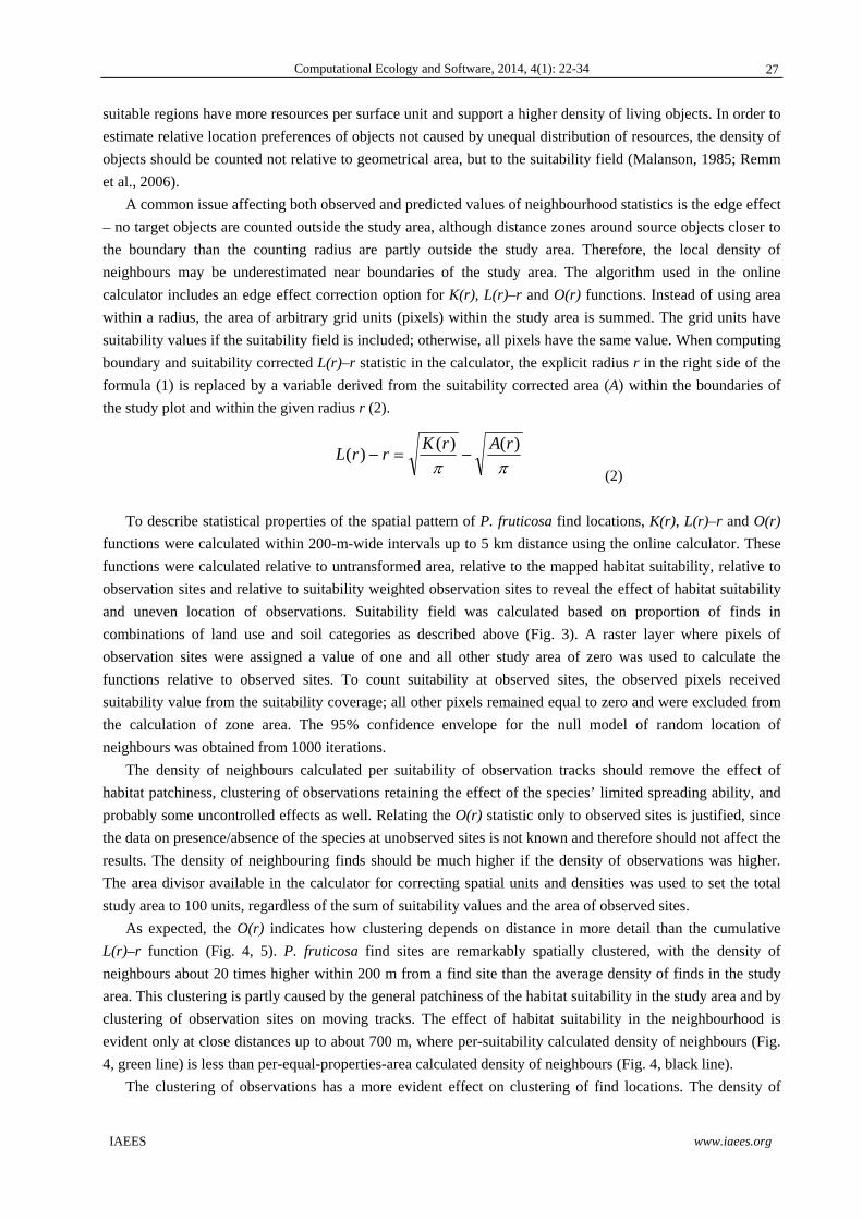
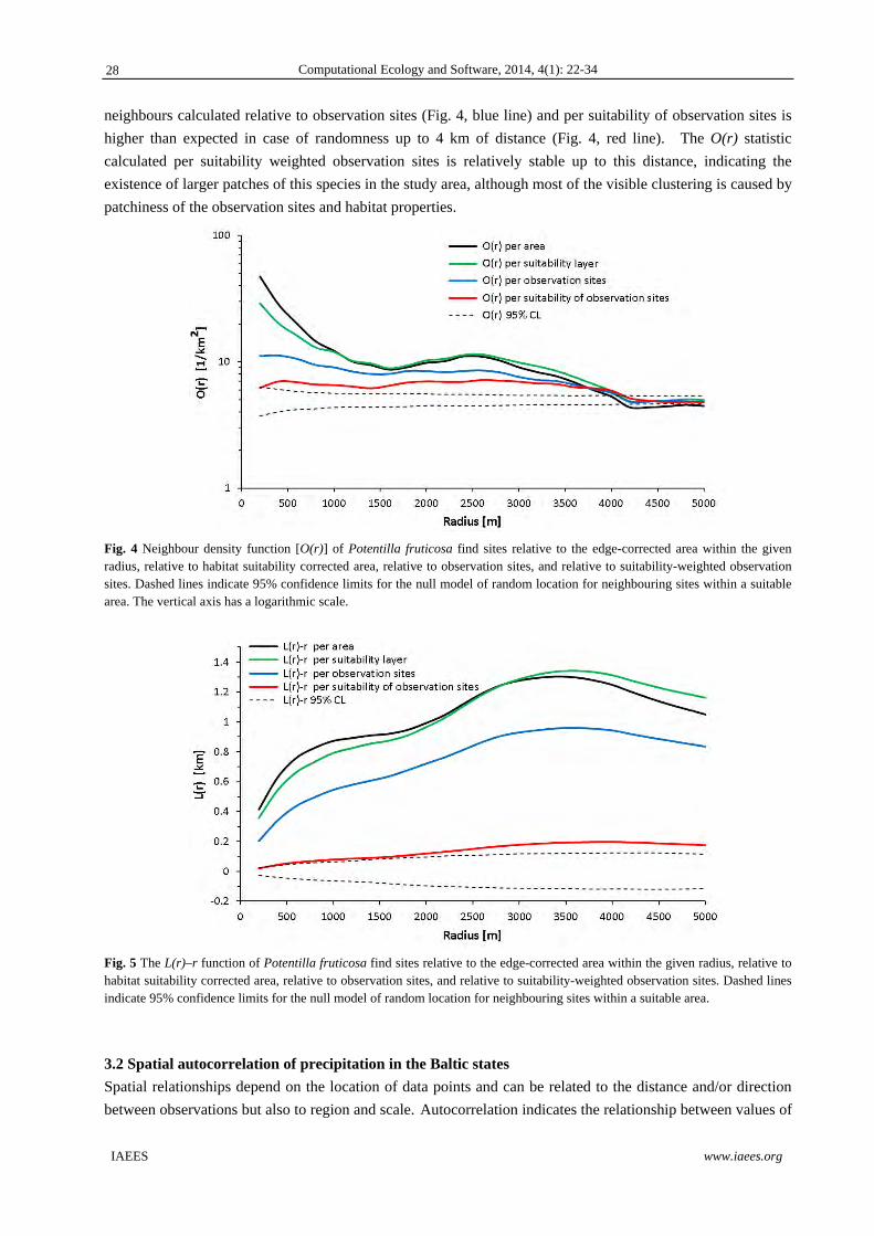
As expected, the O(r) indicates how clustering depends on distance in more detail than the cumulative
L(r)–r function (Fig. 4, 5). P. fruticosa find sites are remarkably spatially clustered, with the density of
neighbours about 20 times higher within 200 m from a find site than the average density of finds in the study
area. This clustering is partly caused by the general patchiness of the habitat suitability in the study area and by
clustering of observation sites on moving tracks. The effect of habitat suitability in the neighbourhood is
evident only at close distances up to about 700 m, where per-suitability calculated density of neighbours (Fig.
4, green line) is less than per-equal-properties-area calculated density of neighbours (Fig. 4, black line).
The clustering of observations has a more evident effect on clustering of find locations. The density of
)()(
)(rArK
rrL
27
Computational Ecology and Software, 2014, 4(1): 22-34
IAEES www.iaees.org
neighbours calculated relative to observation sites (Fig. 4, blue line) and per suitability of observation sites is
higher than expected in case of randomness up to 4 km of distance (Fig. 4, red line). The O(r) statistic
calculated per suitability weighted observation sites is relatively stable up to this distance, indicating the
existence of larger patches of this species in the study area, although most of the visible clustering is caused by
patchiness of the observation sites and habitat properties.
Fig. 4 Neighbour density function [O(r)] of Potentilla fruticosa find sites relative to the edge-corrected area within the given radius, relative to habitat suitability corrected area, relative to observation sites, and relative to suitability-weighted observation sites. Dashed lines indicate 95% confidence limits for the null model of random location for neighbouring sites within a suitable area. The vertical axis has a logarithmic scale.
Fig. 5 The L(r)–r function of Potentilla fruticosa find sites relative to the edge-corrected area within the given radius, relative to habitat suitability corrected area, relative to observation sites, and relative to suitability-weighted observation sites. Dashed lines indicate 95% confidence limits for the null model of random location for neighbouring sites within a suitable area.
3.2 Spatial autocorrelation of precipitation in the Baltic states
Spatial relationships depend on the location of data points and can be related to the distance and/or direction
between observations but also to region and scale. Autocorrelation indicates the relationship between values of
28
Computational Ecology and Software, 2014, 4(1): 22-34
IAEES www.iaees.org
the same variable. It can be both positive, meaning a higher distance-related similarity than expected from
random placement of values, and negative, meaning dissimilarity compared to spatial randomness. As an
analogue to spatial relationships, temporal autocorrelation and correlation depend on difference and direction
in time.
As a rule, close observations tend to be similar because they are affected by the same spatially continuous
factors. If spatial phenomena are recorded, interrelated close data points add less new knowledge than an
independent observation. Measuring autocorrelation is essential to estimate the effect of spatial continuity and
to estimate at which distance the observations can be considered to be independent, as classical statistical
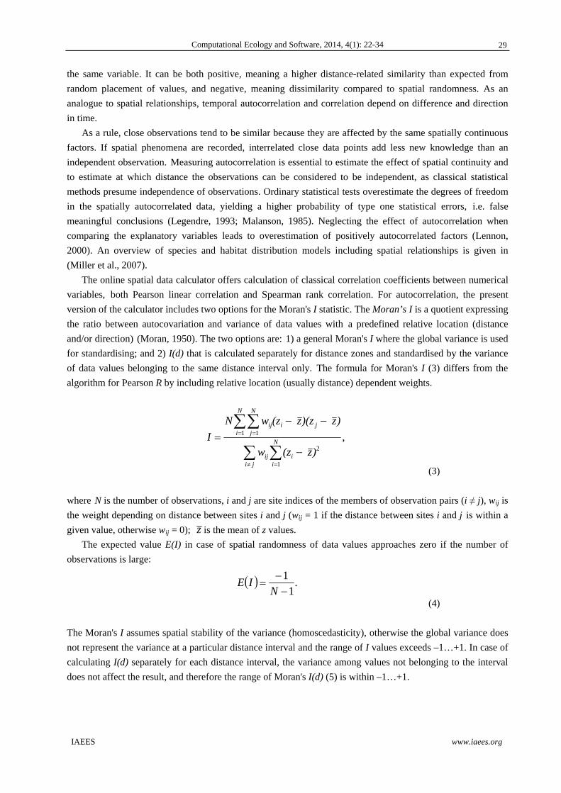
methods presume independence of observations. Ordinary statistical tests overestimate the degrees of freedom
in the spatially autocorrelated data, yielding a higher probability of type one statistical errors, i.e. false
meaningful conclusions (Legendre, 1993; Malanson, 1985). Neglecting the effect of autocorrelation when
comparing the explanatory variables leads to overestimation of positively autocorrelated factors (Lennon,
2000). An overview of species and habitat distribution models including spatial relationships is given in
(Miller et al., 2007).
The online spatial data calculator offers calculation of classical correlation coefficients between numerical
variables, both Pearson linear correlation and Spearman rank correlation. For autocorrelation, the present
version of the calculator includes two options for the Moran's I statistic. The Moran’s I is a quotient expressing
the ratio between autocovariation and variance of data values with a predefined relative location (distance
and/or direction) (Moran, 1950). The two options are: 1) a general Moran's I where the global variance is used
for standardising; and 2) I(d) that is calculated separately for distance zones and standardised by the variance
of data values belonging to the same distance interval only. The formula for Moran's I (3) differs from the
algorithm for Pearson R by including relative location (usually distance) dependent weights.
(3)
where N is the number of observations, i and j are site indices of the members of observation pairs (i ≠ j), wij is
the weight depending on distance between sites i and j (wij = 1 if the distance between sites i and j is within a
given value, otherwise wij = 0); z is the mean of z values.
The expected value E(I) in case of spatial randomness of data values approaches zero if the number of
observations is large:
(4)
The Moran's I assumes spatial stability of the variance (homoscedasticity), otherwise the global variance does
not represent the variance at a particular distance interval and the range of I values exceeds –1…+1. In case of
calculating I(d) separately for each distance interval, the variance among values not belonging to the interval
does not affect the result, and therefore the range of Moran's I(d) (5) is within –1…+1.
,
1
2
1 1
N
ii
jiij
N
i
N
jjiij
)z (zw
)z )(zz (zwN
I
.1
1
N
IE
29
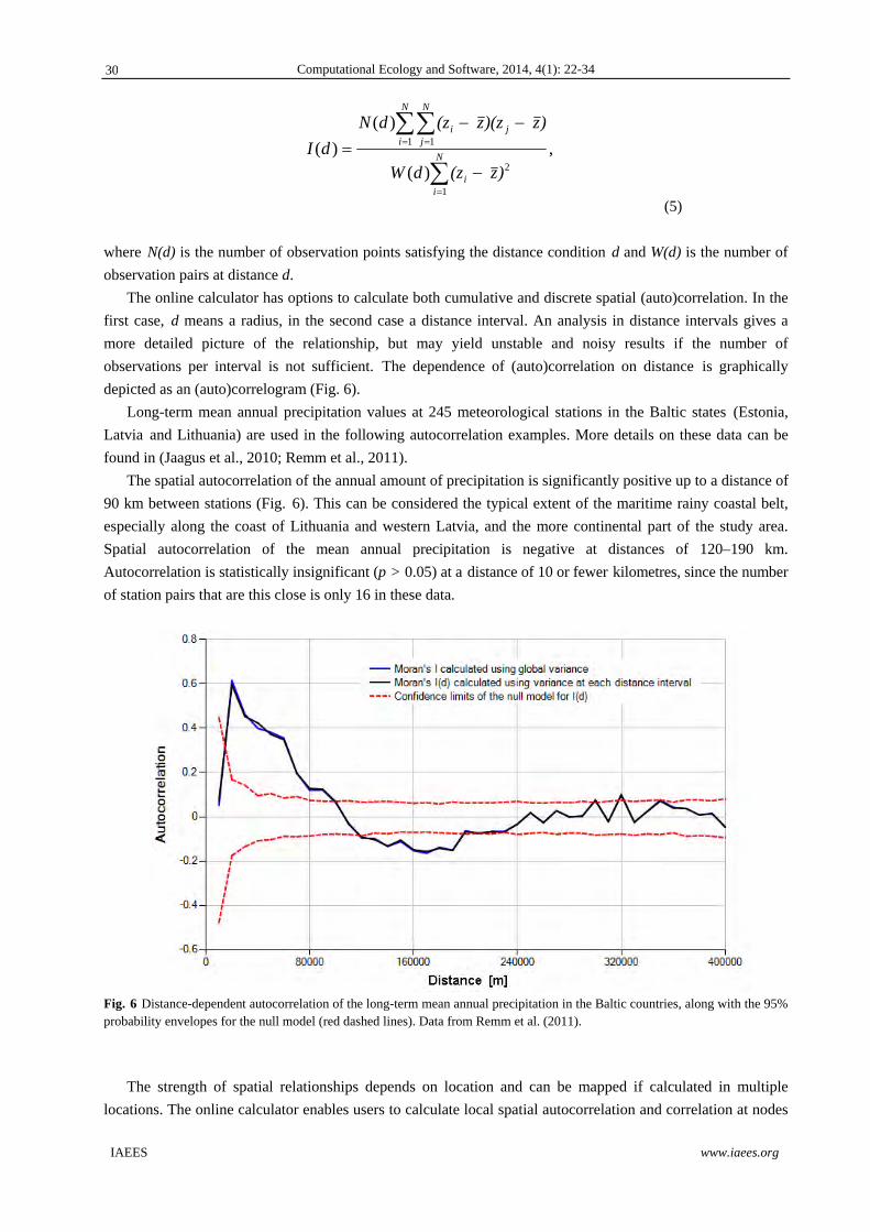
Computational Ecology and Software, 2014, 4(1): 22-34
IAEES www.iaees.org
(5)
where N(d) is the number of observation points satisfying the distance condition d and W(d) is the number of
observation pairs at distance d.
The online calculator has options to calculate both cumulative and discrete spatial (auto)correlation. In the
first case, d means a radius, in the second case a distance interval. An analysis in distance intervals gives a
more detailed picture of the relationship, but may yield unstable and noisy results if the number of
observations per interval is not sufficient. The dependence of (auto)correlation on distance is graphically
depicted as an (auto)correlogram (Fig. 6).
Long-term mean annual precipitation values at 245 meteorological stations in the Baltic states (Estonia,
Latvia and Lithuania) are used in the following autocorrelation examples. More details on these data can be
found in (Jaagus et al., 2010; Remm et al., 2011).
The spatial autocorrelation of the annual amount of precipitation is significantly positive up to a distance of
90 km between stations (Fig. 6). This can be considered the typical extent of the maritime rainy coastal belt,
especially along the coast of Lithuania and western Latvia, and the more continental part of the study area.
Spatial autocorrelation of the mean annual precipitation is negative at distances of 120–190 km.
Autocorrelation is statistically insignificant (p > 0.05) at a distance of 10 or fewer kilometres, since the number
of station pairs that are this close is only 16 in these data.
Fig. 6 Distance-dependent autocorrelation of the long-term mean annual precipitation in the Baltic countries, along with the 95% probability envelopes for the null model (red dashed lines). Data from Remm et al. (2011).
The strength of spatial relationships depends on location and can be mapped if calculated in multiple
locations. The online calculator enables users to calculate local spatial autocorrelation and correlation at nodes
,)(
)(
)(
1
2
1 1
N
ii
N
i
N
jji
)z (zdW
)z )(zz (zdN
dI
30
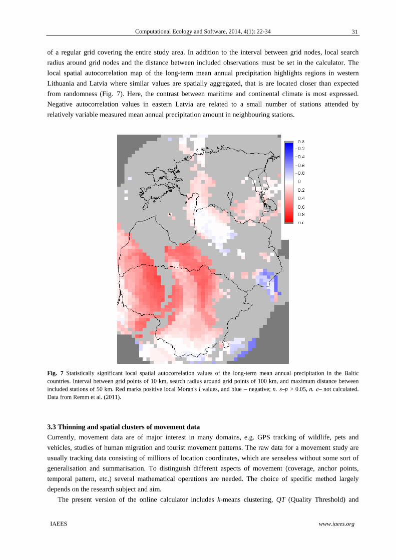
Computational Ecology and Software, 2014, 4(1): 22-34
IAEES www.iaees.org
of a regular grid covering the entire study area. In addition to the interval between grid nodes, local search
radius around grid nodes and the distance between included observations must be set in the calculator. The
local spatial autocorrelation map of the long-term mean annual precipitation highlights regions in western
Lithuania and Latvia where similar values are spatially aggregated, that is are located closer than expected
from randomness (Fig. 7). Here, the contrast between maritime and continental climate is most expressed.
Negative autocorrelation values in eastern Latvia are related to a small number of stations attended by
relatively variable measured mean annual precipitation amount in neighbouring stations.
Fig. 7 Statistically significant local spatial autocorrelation values of the long-term mean annual precipitation in the Baltic countries. Interval between grid points of 10 km, search radius around grid points of 100 km, and maximum distance between included stations of 50 km. Red marks positive local Moran's I values, and blue – negative; n. s–p > 0.05, n. c– not calculated. Data from Remm et al. (2011).
3.3 Thinning and spatial clusters of movement data
Currently, movement data are of major interest in many domains, e.g. GPS tracking of wildlife, pets and
vehicles, studies of human migration and tourist movement patterns. The raw data for a movement study are
usually tracking data consisting of millions of location coordinates, which are senseless without some sort of
generalisation and summarisation. To distinguish different aspects of movement (coverage, anchor points,
temporal pattern, etc.) several mathematical operations are needed. The choice of specific method largely
depends on the research subject and aim.
The present version of the online calculator includes k-means clustering, QT (Quality Threshold) and
31
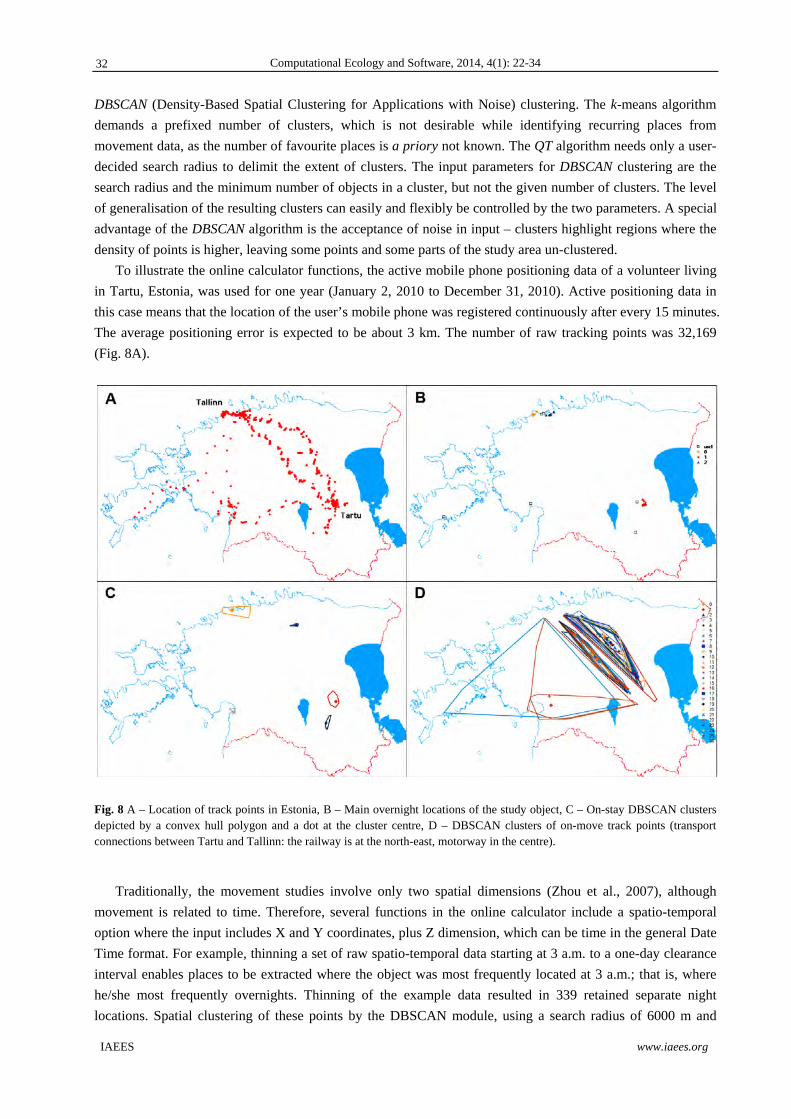
Computational Ecology and Software, 2014, 4(1): 22-34
IAEES www.iaees.org
DBSCAN (Density-Based Spatial Clustering for Applications with Noise) clustering. The k-means algorithm
demands a prefixed number of clusters, which is not desirable while identifying recurring places from
movement data, as the number of favourite places is a priory not known. The QT algorithm needs only a user-
decided search radius to delimit the extent of clusters. The input parameters for DBSCAN clustering are the
search radius and the minimum number of objects in a cluster, but not the given number of clusters. The level
of generalisation of the resulting clusters can easily and flexibly be controlled by the two parameters. A special
advantage of the DBSCAN algorithm is the acceptance of noise in input – clusters highlight regions where the
density of points is higher, leaving some points and some parts of the study area un-clustered.
To illustrate the online calculator functions, the active mobile phone positioning data of a volunteer living
in Tartu, Estonia, was used for one year (January 2, 2010 to December 31, 2010). Active positioning data in
this case means that the location of the user’s mobile phone was registered continuously after every 15 minutes.
The average positioning error is expected to be about 3 km. The number of raw tracking points was 32,169
(Fig. 8A).
Fig. 8 A – Location of track points in Estonia, B – Main overnight locations of the study object, C – On-stay DBSCAN clusters depicted by a convex hull polygon and a dot at the cluster centre, D – DBSCAN clusters of on-move track points (transport connections between Tartu and Tallinn: the railway is at the north-east, motorway in the centre).
Traditionally, the movement studies involve only two spatial dimensions (Zhou et al., 2007), although
movement is related to time. Therefore, several functions in the online calculator include a spatio-temporal
option where the input includes X and Y coordinates, plus Z dimension, which can be time in the general Date
Time format. For example, thinning a set of raw spatio-temporal data starting at 3 a.m. to a one-day clearance
interval enables places to be extracted where the object was most frequently located at 3 a.m.; that is, where
he/she most frequently overnights. Thinning of the example data resulted in 339 retained separate night
locations. Spatial clustering of these points by the DBSCAN module, using a search radius of 6000 m and
32
Computational Ecology and Software, 2014, 4(1): 22-34
IAEES www.iaees.org
cluster size of 30 resulted in three frequent overnight places for this person: at home in Tartu, somewhere in
the capital, Tallinn, and one about 20 km west of Tallinn (Fig. 8B). The other locations can be considered
occasional.
A second exercise was separating two kinds of tracking points and generalising these into two types of
clusters: on-move clusters that reflect the trajectories of movement, and on-stay clusters that indicate locations
where the study object has spent more time. To get on-stay clusters, the search radius along XY plane should
be delimited to a shorter value (6000 m in this case) and the time difference should be at least as long as the
study period. The minimum number of objects in a cluster was set to 30. Most of the track points were
classified as on-stay category at this stage. The rest (515) were considered on-move points, which were
generalised into clusters using a 12-hour maximum time difference and not limiting search radius. The
minimum number of objects in an on-move cluster was set to 5, since in some cases only 5 track points were
recorded during Tallinn–Tartu train travel.
As a result, five on-stay clusters and two on-way clusters were generalised for this person. The largest on-
stay cluster is around the Tartu residence; the on-way clusters represent one-day travel routes (49 times
between the hometown and capital, Tallinn), one tour near Tartu, and three longer trips to western Estonia (Fig.
8C, D).
4 Conclusions
The online calculator introduced above supports a wide range of spatial analysis operations, although, the
application is still merely a calculator primarily developed for teaching purposes. For larger datasets and more
comprehensive studies, special software is needed or should be developed. The code for all functions used in
the online calculator is freely open for assessment, criticism, and development of other applications.
The presented examples of spatial analysis were all calculated using the online calculator. The example
cases yielded the following results.
(1) Spatial analysis of Potentilla fruticosa find locations reveals that the main reasons for the obvious
clustering of finds are the patchiness of suitable habitats and clustering of observation sites. Although the seeds
of this plant are not spreading far, the inherent dispersal-related patchiness has a weaker effect than soil
properties and land use type combined.
(2) Spatial autocorrelation of the annual amount of precipitation at the Baltic meteorological stations is
significantly positive at a distance of 10–90 km between stations.
(3) Spatio-temporal clustering of movement data supports insights into large sets of tracking data,
generalisation and visualisation of movement.
Acknowledgments
The authors thank Markus Unt for participating in code development, colleagues Jaanus Remm for developing
an earlier solution for directional analysis and Ain Kull for advice supporting the present module of directional
analysis in the calculator; and also the proof reader Dirk Lloyd. The development of this calculator was
financially supported by the Estonian Ministry of Education and Research (Project IUT 2-16).
References
Condit R, Ashton PS, Baker P, et al. 2000. Spatial patterns in the distribution of tropical tree species. Science,
288(5470): 1414-1418
Elkington TT. 1969. Cytotaxonomic variation in Potentilla fruticosa L. New Phytologist, 68(1): 151-160
33
Computational Ecology and Software, 2014, 4(1): 22-34
IAEES www.iaees.org
He F, Duncan RP. 2000. Density-dependent effects on tree survival in an old-growth Douglas fir forest.
Journal of Ecology, 88(4): 676-688
Jaagus J, Briede A, Rimkus E, Remm K. 2010. Precipitation pattern in the Baltic countries under the influence
of large-scale atmospheric circulation and local landscape factors. International Journal of Climatology,
30(5): 705-720
Kotta J, Remm K, Vahtmäe E, et al. 2013. In-air spectral signatures of the Baltic Sea macrophytes and their
statistical separability. Journal of Applied Remote Sensing (submitted manuscript).
Law R, Illian J, Burslem DFRP, et al. 2009. Ecological information from spatial patterns of plants: insights
from point process theory. Journal of Ecology, 97(4): 616–628
Legendre P. 1993. Spatial autocorrelation: trouble or new paradigm? Ecology, 74(6): 1659-1673
Leht M, Reier Ü. 1999. Origin, chromosome number and reproduction biology of Potentilla fruticosa
(Rosaceae) in Estonia and Latvia. In: Chorological Problems in the European Flora. (Uotila P, ed).
Proceedings of the VIII meeting of the Committee for Mapping the Flora of Europe. 191-196, Helsinki,
Finland
Lennon JJ. 2000. Red-shifts and red herrings in geographical ecology. Ecography, 23(1): 101-113
Malanson GP. 1985. Spatial autocorrelation and distributions of plant species on environmental gradients.
Oikos, 45(2): 278-280
Miller J, Franklin J, Aspinall R. 2007. Incorporating spatial dependence in predictive vegetation models.
Ecological Modelling, 202(3-4): 225-242
Moran PAP. 1950. Notes on continous stochastic phenomena. Biometrika, 37(1-2): 17-23
Remm J, Lõhmus A, Remm K. 2006. Tree cavities in riverine forests: what determines their occurrence and
use by hole-nesting passerines? Forest Ecology and Management, 221(1-3): 267-277
Remm K, Jaagus J, Briede A, et al. 2011. Interpolative mapping of mean precipitation in the Baltic countries
by using landscape characteristics. Estonian Journal of Earth Sciences, 60(3): 172-190
Remm K, Kelviste T. 2011. Constud Tutorial. University of Tartu, Chair of Geoinformatics and Cartography,
Tartu, Estonia
Remm K, Luud A. 2003. Regression and point pattern models of moose distribution in relation to habitat
distribution and human influence in Ida-Viru county, Estonia. Journal for Nature Conservation, 11(3): 197-
211
Remm M, Remm K. 2008. Case-based estimation of the risk of enterobiasis. Artificial Intelligence in Medicine,
43(3): 167-177
Ripley BD. 1976. The second-order analysis of stationary point processes. Journal of Applied Probability,
13(2): 225-266
Ripley BD. 1977. Modelling spatial patterns. Journal of the Royal Statistical Society, B 39(2): 172-212
Ripley BD. 1981. Spatial Statistics. Wiley, New York, USA
Wiegand T, Moloney KA. 2004. Rings, circles and null-models for point pattern analysis in ecology. Oikos,
104(2): 209-229
Wiegand T, Moloney KA, Naves J, Knauer F. 1999. Finding the missing link between landscape structure and
population dynamics: a spatially explicit perspective. The American Naturalist, 154(6): 605-627
Zhang WJ. 2010. Computational Ecology: Artificial Neural Networks and Their Applications. World
Scientific, Singapore
Zhou C, Bhatnagar N, Shekhar S, et al. 2007. Mining Personally Important Places from GPS Tracks. Data
Engineering Workshop, IEEE 23rd International Conference, 517-526
34
Computational Ecology and Software, 2014, 4(1): 35-46
IAEES www.iaees.org
Article
Global behavior of an anti-competitive system of fourth-order rational
difference equations
A. Q. Khan1, Q. Din1, M. N. Qureshi1, T. F. Ibrahim2,3 1Department of Mathematics, University of Azad Jammu & Kashmir, Muzaffarabad, Pakistan 2Department of Mathematics, Faculty of Sciences and Arts King Khalid University, Abha, Saudi Arabia 3Permanent address: Department of Mathematics, Faculty of Sciences Mansoura University, Mansoura 35516, Egypt
E-mail:[email protected],[email protected],[email protected],[email protected]
Received 22 October 2013; Accepted 28 November 2013; Published online 1 March 2014
Abstract
In the present work, we study the qualitative behavior of an anti-competitive system of fourth-order rational
difference equations. More precisely, we study the local asymptotic stability, global character of the unique
equilibrium point, and the rate of convergence of the positive solutions of the given system. Some numerical
examples are given to verify our theoretical results.
Keywords system of rational difference equations; stability; global character; rate of convergence.
1 Introduction
Difference equations or discrete dynamical systems are diverse field which impact almost every branch of pure
and applied mathematics. Every dynamical system determines a difference equation and vice
versa. Recently, there has been great interest in studying difference equations systems. One of the reasons for
this is a necessity for some techniques which can be used in investigating equations arising in mathematical
models describing real life situations in many applied sciences. The theory of discrete dynamical systems and
difference equations developed greatly during the last twenty-five years of the twentieth century. Applications
of discrete dynamical systems and difference equations have appeared recently in many areas. The theory of
difference equations occupies a central position in applicable analysis. There is no doubt that the theory of
difference equations will continue to play an important role in mathematics as a whole. Nonlinear difference
equations of order greater than one are of paramount importance in applications. Such equations also appear
naturally as discrete analogues and as numerical solutions of differential and delay differential equations which
model various diverse phenomena in biology, ecology, physiology, physics, engineering, economics,
probability theory, genetics, psychology and resource management. It is very interesting to investigate the
Computational Ecology and Software ISSN 2220721X URL: http://www.iaees.org/publications/journals/ces/onlineversion.asp RSS: http://www.iaees.org/publications/journals/ces/rss.xml Email: [email protected] EditorinChief: WenJun Zhang Publisher: International Academy of Ecology and Environmental Sciences
Computational Ecology and Software, 2014, 4(1): 35-46
IAEES www.iaees.org
behavior of solutions of a system of higher-order rational difference equations and to discuss the local
asymptotic stability of their equilibrium points. Systems of rational difference equations have been studied by
several authors. Especially there has been a great interest in the study of the attractivity of the solutions of such
systems. For more results for the systems of difference equations, we refer the interested reader to Cinar
(2004), Stevic (2012a, b), Bajo and Liz (2011), Kalabusic et al. (2009, 2011), Kurbanli (2011), Kurbanli et al.
(2011), Touafek and Elsayed (2012a, b), Elsayed and Ibrahim (in press), Din (a, b; in press).
Zhang et al. (2012) studied the dynamics of a system of rational third-order difference equation:
, , 0,1, .
Din et al. (2012) investigated the dynamics of a system of fourth-order rational difference equations
∏ ,
∏, 0,1, ,
Our aim in this paper is to investigate the qualitative behavior of an anti-competitive system of fourth order
rational difference equations
∏ ,
∏, 0,1, , (1)
where the parameters , , , , , and initial conditions , , , , , , , are
positive real numbers. This paper is natural extension of (Shojaei et al., 2009; Din et al., 2012; Zhang et al.,
2012).
Let us consider eight-dimensional discrete dynamical system of the form:
, , , , , , , , , , , , , , , , 0,1, , (2)
where : and : are continuously differentiable functions and , are some
intervals of real numbers. Furthermore, a solution , of system (2) is uniquely determined by
initial conditions , for 3, 2, 1,0 . Along with the system (2) we consider the
corresponding vector map
, , , , , , , , , .
An equilibrium point of system (2) is a point , that satisfies
, , , , , , ,
, , , , , , ,
The point , is also called a fixed point of the vector map .
Definition 1. Let , be an equilibrium point of the system (2).
(i) An equilibrium point , is said to be stable if for every 0 there exists 0 such
thatfor every initial conditions , , 3, 2, 1,0 if ∑ , ,
implies , , for all 0, where · is usual Euclidian norm in .
(ii) An equilibrium point , is said to be unstable if it is not stable.
(iii) An equilibrium point , is said to be asymptotically stable if there exists 0 such that
∑ , , and , , as ∞.
(iv) An equilibrium point , is called global attractor if , , as ∞. (v) An equilibrium point , is called asymptotic global attractor if it is a global attractor andstable.
Definition 2. Let , be an equilibrium point of a map
, , , , , , , , ,
where and are continuously differentiable functions at , . The linearized system of (2) about the
36
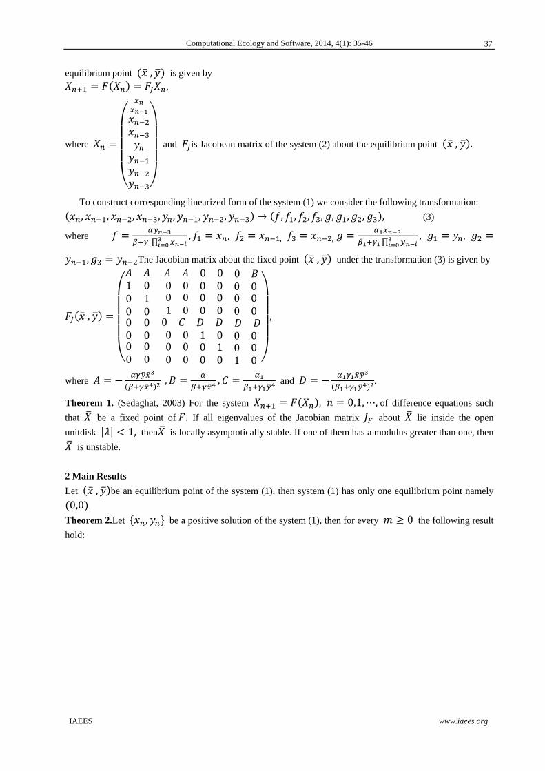
Computational Ecology and Software, 2014, 4(1): 35-46
IAEES www.iaees.org
equilibrium point , is given by
,
where and is Jacobean matrix of the system (2) about the equilibrium point , .
To construct corresponding linearized form of the system (1) we consider the following transformation:
, , , , , , , , , , , , , , , (3)
where ∏
, , , , ∏, ,
, The Jacobian matrix about the fixed point , under the transformation (3) is given by
,
0 0 01 0 0 0 0 0 0 0000000
100000
0 0 0 0 0 01 0 0 0 0 000 0 1 0 0 00 0 0 1 0 00 0 0 0 1 0
,
where , , and .
Theorem 1. (Sedaghat, 2003) For the system , 0,1, , of difference equations such
that be a fixed point of . If all eigenvalues of the Jacobian matrix about lie inside the open
unitdisk | | 1, then is locally asymptotically stable. If one of them has a modulus greater than one, then
is unstable.
2 Main Results
Let , be an equilibrium point of the system (1), then system (1) has only one equilibrium point namely
0,0 .
Theorem 2.Let , be a positive solution of the system (1), then for every 0 the following result
hold:
37
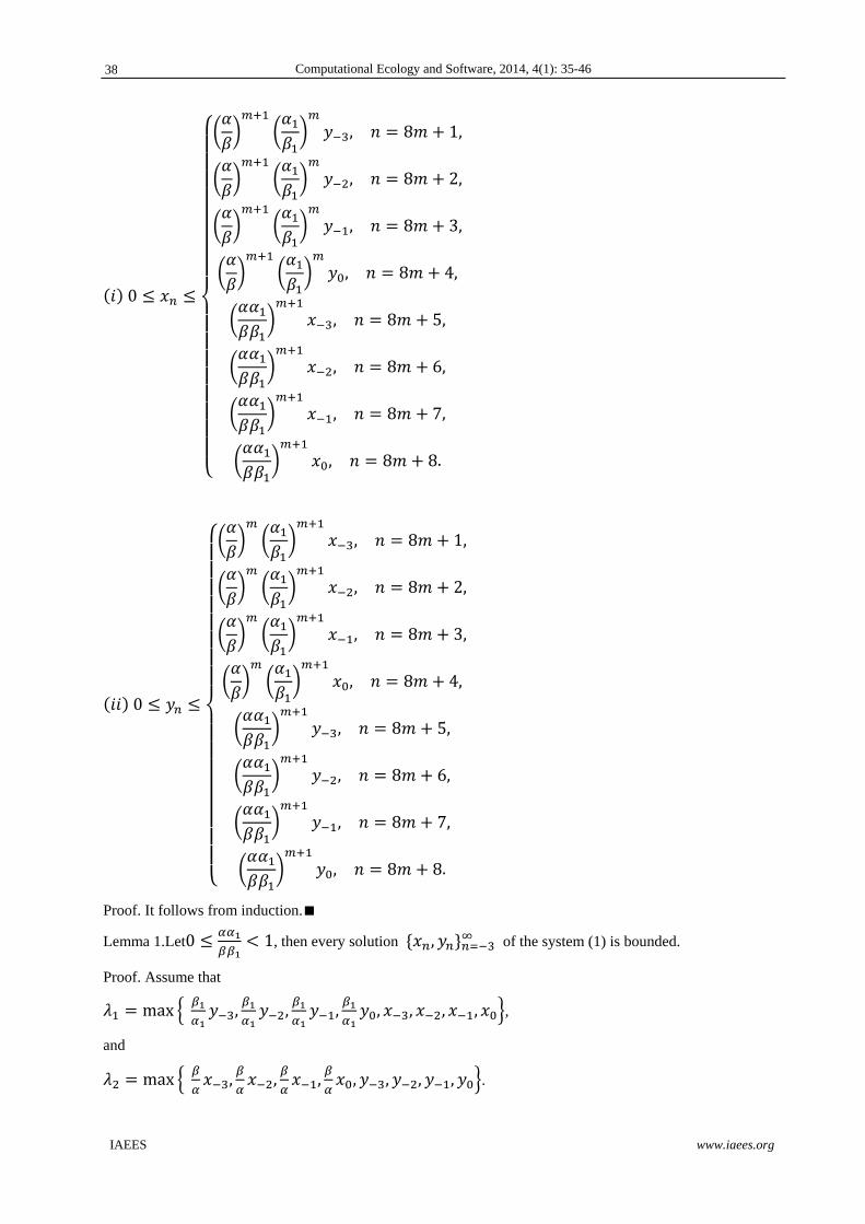
Computational Ecology and Software, 2014, 4(1): 35-46
IAEES www.iaees.org
0
, 8 1,
, 8 2,
, 8 3,
, 8 4,
, 8 5,
, 8 6,
, 8 7,
, 8 8.
0
, 8 1,
, 8 2,
, 8 3,
, 8 4,
, 8 5,
, 8 6,
, 8 7,
, 8 8.
Proof. It follows from induction.
Lemma 1.Let0 1, then every solution , of the system (1) is bounded.
Proof. Assume that
max , , , , , , , ,
and
max , , , , , , , .
38
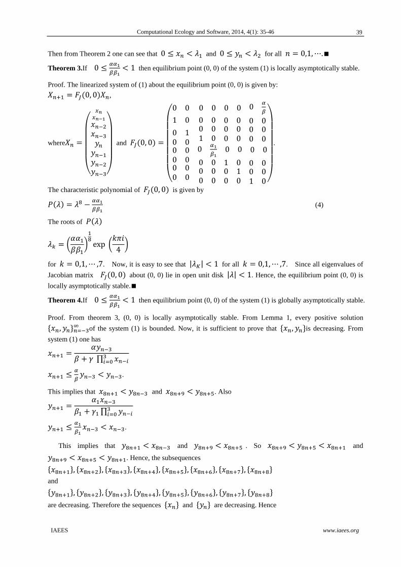
Computational Ecology and Software, 2014, 4(1): 35-46
IAEES www.iaees.org
Then from Theorem 2 one can see that 0 and 0 for all 0,1, .
Theorem 3.If 0 1 then equilibrium point (0, 0) of the system (1) is locally asymptotically stable.
Proof. The linearized system of (1) about the equilibrium point (0, 0) is given by:
0, 0 ,
where and 0, 0
0 0 0 0 0 0 0
1 0 0 0 0 0 0 0
000000
100000
0 0 0 0 0 01 0 0 0 0 00 0 0 0 0
0 0 1 0 0 00 0 0 1 0 00 0 0 0 1 0
.
The characteristic polynomial of 0, 0 is given by
(4)
The roots of
exp 4
for 0,1, ,7. Now, it is easy to see that | | 1 for all 0,1, ,7. Since all eigenvalues of
Jacobian matrix 0, 0 about (0, 0) lie in open unit disk | | 1. Hence, the equilibrium point (0, 0) is
locally asymptotically stable.
Theorem 4.If 0 1 then equilibrium point (0, 0) of the system (1) is globally asymptotically stable.
Proof. From theorem 3, (0, 0) is locally asymptotically stable. From Lemma 1, every positive solution
, of the system (1) is bounded. Now, it is sufficient to prove that , is decreasing. From
system (1) one has
∏
.
This implies that and . Also
∏
.
This implies that and . So and
. Hence, the subsequences
, , , , , , ,
and
, , , , , , ,
are decreasing. Therefore the sequences and are decreasing. Hence
39
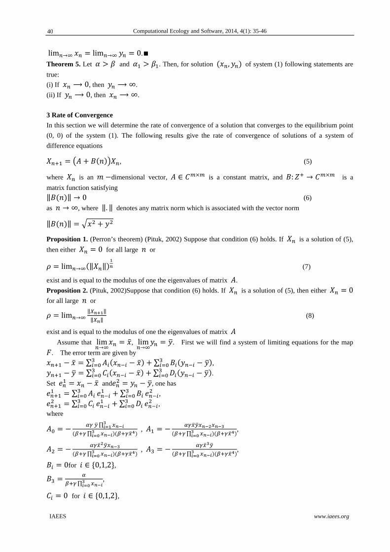
Computational Ecology and Software, 2014, 4(1): 35-46
IAEES www.iaees.org
lim lim 0.
Theorem 5. Let and . Then, for solution , of system (1) following statements are
true:
(i) If 0, then ∞.
(ii) If 0, then ∞.
3 Rate of Convergence
In this section we will determine the rate of convergence of a solution that converges to the equilibrium point
(0, 0) of the system (1). The following results give the rate of convergence of solutions of a system of
difference equations
, (5)
where is an dimensional vector, is a constant matrix, and : is a
matrix function satisfying
0 (6)
as ∞, where . denotes any matrix norm which is associated with the vector norm
Proposition 1. (Perron’s theorem) (Pituk, 2002) Suppose that condition (6) holds. If is a solution of (5),
then either 0 for all large or
lim (7)
exist and is equal to the modulus of one the eigenvalues of matrix .
Proposition 2. (Pituk, 2002)Suppose that condition (6) holds. If is a solution of (5), then either 0
for all large or
lim (8)
exist and is equal to the modulus of one the eigenvalues of matrix
Assume that lim , lim . First we will find a system of limiting equations for the map
. The error term are given by
∑ ∑ ,
∑ ∑ .
Set and , one has
∑ ∑ ,
∑ ∑ ,
where
∏
∏ ,
∏,
∏ ,
∏,
0for 0,1,2 ,
∏,
0 for 0,1,2 ,
40
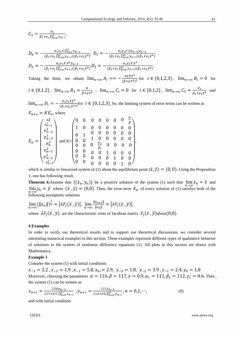
Computational Ecology and Software, 2014, 4(1): 35-46
IAEES www.iaees.org
∏,
∏
∏,
∏,
∏,
∏.
Taking the limit, we obtain lim for 0,1,2,3 , lim 0 for
0,1,2 , lim , lim 0 for 0,1,2 , lim and
lim for 0,1,2,3 . So, the limiting system of error terms can be written as
, where
and K=
0 0 0 0 0 0 0
1 0 0 0 0 0 0 0
000000
100000
0 0 0 0 0 01 0 0 0 0 00 0 0 0 0
0 0 1 0 0 00 0 0 1 0 00 0 0 0 1 0
,
which is similar to linearized system of (1) about the equilibrium point ( , 0, 0 . Using the Proposition
1, one has following result.
Theorem 6.Assume that , be a positive solution of the system (1) such that lim and
lim where , 0,0 . Then, the error term of every solution of (1) satisfies both of the
following asymptotic relations
lim , , lim , ,
where , are the characteristic roots of Jacobian matrix , about 0,0 .
4 Examples
In order to verify our theoretical results and to support our theoretical discussions, we consider several
interesting numerical examples in this section. These examples represent different types of qualitative behavior
of solutions to the system of nonlinear difference equations (1). All plots in this section are drawn with
Mathematica.
Example 1
Consider the system (1) with initial conditions
2.2 , 1.9 , 5.8, , 2.9, 1.8, 3.9 , 2.4, 1.8 .
Moreover, choosing the parameters 116, 117, 0.9, 111, 112, 0.6. Then ,
the system (1) can be written as
. ∏ ,
. ∏, 0,1, , (9)
and with initial condition
41
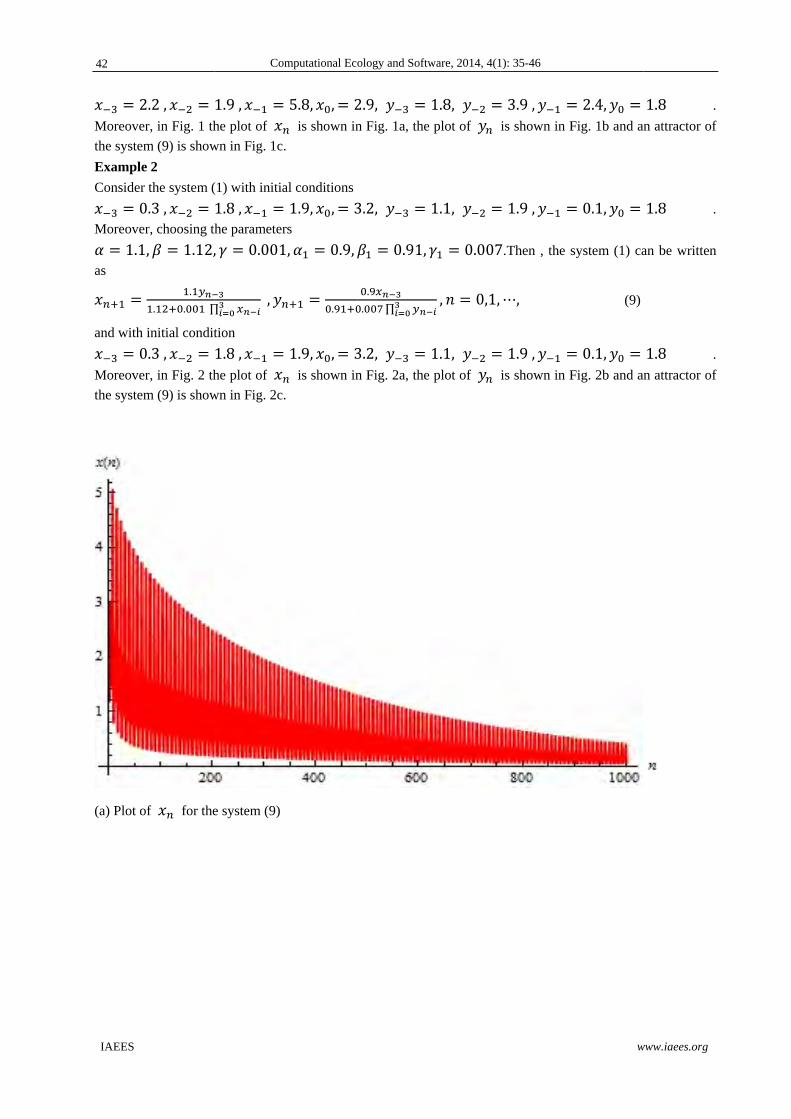
IAEES
2Moreove
the syste
Example
Consider
0Moreove
1.1as
and with
0Moreove
the syste
(a) Plot o
2.2 ,er, in Fig. 1 th
m (9) is show
e 2
r the system (
0.3 ,er, choosing th
1, 1.12,
.
. . ∏
initial condit
0.3 ,er, in Fig. 2 th
m (9) is show
of for the
Com
1.9 ,he plot of
wn in Fig. 1c.
(1) with initia
1.8 ,he parameter
, 0.001
∏ ,
tion
1.8 ,he plot of
wn in Fig. 2c.
e system (9)
mputational Eco
5.8, , 2 is shown in
al conditions
1.9, , 3rs
, 0.9,
.
1.9, , 3 is shown in
ology and Softw
2.9,n Fig. 1a, the
3.2,
0.91,
.
. ∏
3.2,n Fig. 2a, the
ware, 2014, 4(1
1.8,e plot of
1.1,
0.007
, 0,1,
1.1,e plot of
1): 35-46
3.9 ,is shown in F
1.9 ,
7.Then , the s
,
1.9 ,is shown in F
w
2.4,Fig. 1b and a
0.1,
system (1) ca
(9)
0.1,Fig. 2b and a
www.iaees.org
1.8 .
n attractor of
1.8 .
an be written
1.8 .
n attractor of
.
f
.
n
.
f
42

IAEES
(b) Plot o
(c) An at
of for the
ttractor for th
Com
e system (9)
he system (9)
mputational Eco
Fig. 1
ology and Softw
1 Plots for the s
ware, 2014, 4(1
system (9).
1): 35-46
w
www.iaees.org
43
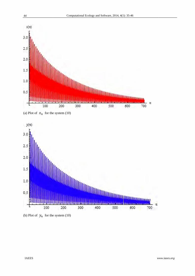
IAEES
(a) Plot o
(b) Plot o
of for the
of for the
Com
e system (10)
e system (10)
mputational Eco
)
)
ology and Softw
ware, 2014, 4(1
1): 35-46
w
www.iaees.org
44
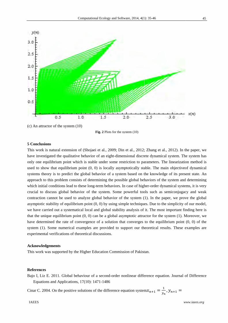
IAEES
(c) An at
5 Conclu
This wor
have inv
only one
used to s
systems
approach
which in
crucial t
contracti
asymptot
we have
that the u
have det
system (
experime
Acknow
This wor
Referenc
Bajo I, L
Equa
Cinar C.
ttractor of the
usions
rk is natural e
estigated the
e equilibrium
show that eq
theory is to p
h to this prob
itial condition
o discuss gl
on cannot be
tic stability o
carried out a
unique equili
termined the
(1). Some nu
ental verificat
wledgements
rk was suppor
ces
Liz E. 2011. G
ations and Ap
2004. On the
Com
e system (10)
extension of
qualitative b
point which
quilibrium po
predict the g
lem consists
ns lead to the
obal behavio
e used to ana
of equilibrium
a systematica
ibrium point
rate of conv
umerical exam
tions of theor
rted by the H
Global behav
pplications, 17
e positive solu
mputational Eco
Fig. 2
(Shojaei et a
behavior of an
h is stable und
oint (0, 0) is
lobal behavio
of determini
ese long-term
or of the sys
alyze global
m point (0, 0)
l local and gl
(0, 0) can be
vergence of a
mples are pr
retical discuss
Higher Educat
viour of a sec
7(10): 1471-1
utions of the
ology and Softw
2 Plots for the sy
al., 2009; Din
n eight-dimen
der some res
locally asym
or of a system
ng the possib
m behaviors. In
stem. Some p
behavior of
by using sim
lobal stability
e a global asy
a solution tha
rovided to su
sions.
tion Commiss
cond-order no
1486
difference eq
ware, 2014, 4(1
ystem (10)
n et al., 2012;
nsional discre
triction to pa
mptotically sta
m based on t
ble global beh
n case of high
powerful too
the system (
mple technique
y analysis of
ymptotic attra
at converges
upport our th
sion of Pakist
onlinear diffe
quation system
1): 35-46
; Zhang et al
ete dynamica
arameters. Th
able. The ma
the knowledg
haviors of the
her-order dyn
ols such as s
1). In the pa
es. Due to the
it. The most
actor for the s
to the equili
heoretical resu
tan.
erence equati
m
w
., 2012). In t
al system. Th
he linearizatio
ain objectiveo
ge of its pres
e system and
namical syste
semiconjugac
aper, we prov
e simplicity o
important fin
system (1). M
ibrium point
ults. These e
ion. Journal o
,
www.iaees.org
the paper, we
he system has
on method is
of dynamical
ent state. An
d determining
ems, it is very
cy and weak
ve the global
of our model,
nding here is
Moreover, we
(0, 0) of the
examples are
of Difference
e
s
s
l
n
g
y
k
l
,
s
e
e
e
e
45
Computational Ecology and Software, 2014, 4(1): 35-46
IAEES www.iaees.org
. Applied Mathematics and Computation, 158: 303-305
Din Q, Donchev T. 2013.Global character of a host-parasite model. Chaos, Solitons and Fractal,54:1-7
Din Q, Donchev T. 2013.Global stability of a population model.Chaos, Solitons and Fractal, in press
Din Q. Dynamics of a discrete Lotka-Volterra model. Advances in Difference Equations, doi: 10.1186/1687-
1847-2013-95
Din Q. Global character of a rational difference equation. Thai Journal of Mathematics, in press (a)
Din Q. On a system of rational difference equation. Demonstratio Mathematica, in press (b)
Din Q, Khan AQ, Qureshi MN. 2013. Qualitative behavior of a host-pathogen model, Advances in Difference
Equations, doi:10.1186/1687-1847-2013-263
Din Q, Qureshi MN, Khan AQ. 2012. Dynamics of a fourth-order system of rational difference equations.
Advances in Difference Equations, doi:10.1186/1687-1847-2012-216
Elsayed EM, Ibrahim TF. Solutions and periodicity of a rational recursive sequences of order five. Bulletin of
the Malaysian Mathematical Sciences Society, in press
Grove EA, Ladas G. 2004. Periodicities in Nonlinear Difference Equations, Chapman and Hall/CRC Press,
Boca Raton, USA
Kalabusic S, Kulenovic MRS, Pilav E. 2009. Global dynamics of a competitive system ofrational difference
equations in the plane. Advances in Difference Equations, 1-30 (132802)
Kalabusic S, Kulenovic MRS, Pilav E. 2011. Dynamics of a two-dimensional system of rationaldifference
equations of Leslie--Gower type. Advances in Difference Equations, 1-29 (doi: 10.1186/1687-1847-2011-
29)
Kurbanli AS. 2011. On the behavaior of positive solutions of the system of rational difference
, , ,. Advances in Difference Equations, 40
Kurbanli AS, Cinar C, Yalcinkaya I. 2011. On the behavior of positive solutions of the system ofrational
difference equations , . Mathematical and Computer Modelling, 53:
1261-1267
Pituk M. 2002. More on Poincare’s and Perron’s theorems for difference equations. Journal of Difference
Equations and Applications, 8: 201-216
Sedaghat H. 2003. Nonlinear Difference Equations: Theory With Applications To Social Science Models.
Kluwer Academic Publishers, Dordrecht, Netherlands
Shojaei M, Saadati R, Adibi H. 2009. Stability and periodic character of a rational third order difference
equation. Chaos, Solitons and Fractals, 39: 1203-1209
Stevic S. 2012a. On a third-order system of difference equations. Applied Mathematics and Computation, 218,
7649-7654
Stevic S. 2012b. On some solvable systems of difference equations. Applied Mathematics and Computation,
218: 5010-5018
Touafek N, Elsayed EM. 2012a. On the periodicity of some systems of nonlinear difference equations. Bulletin
Mathematique de la Societe des Sciences Mathematiques de Roumanie, 2: 217-224
Touafek N, Elsayed EM. 2012b. On the solutions of systems of rational difference equations. Mathematical
and Computer Modelling, 55: 1987-1997
Zhang Q, Yang L, Liu J. 2012. Dynamics of a system of rational third order difference equation. Advances in
Difference Equations, 1-8 (doi: 10.1186/1687-1847-2012-136)
46
Computational Ecology and Software, 2014, 4(1): 47-62
IAEES www.iaees.org
Article
Effect of land uses of Huai Lam Kradon Sub-watershed on quantifying
soil carbon potential with process base model
Chattanong Podong1, Roongreang Poolsiri2
1Department of Conservation, Faculty of Forestry, Kasetsart University, Chatuchak, Bangkok, Thailand 10900 2Department of Sivilculture, Faculty of Forestry, Kasetsart University, Chatuchak, Bangkok, Thailand 10900
E-mail: [email protected]
Received 19 October 2013; Accepted 25 November 2013; Published online 1 March 2014
Abstract
The study the effect of land use on soil carbon is importantly for the future management of greenhouse gases
and climate change, and soil carbon budget is one activity mention of the United Nations Framework
Convention on Climate Change (UNFCCC) for decreasing effect from climate change. Previous studies based
on field observations have provided direct information about soil carbon storage and fluxes at specific sites,
but soil carbon is highly dynamic in space and time and that is driven by complex combinations of hydrology,
soil vegetation and management condition. The observation results was soil carbon higher in mixed deciduous
forest 17,472.30 Kg C ha-1 than para rubber plantation 8,304.52 Kg C ha-1 at depth 0-5 cm and at depth 5-20
cm 8,304.52 Kg C ha-1 and 6,776.65, respectively. The DNDC model has shown that it can perform well in its
representation of the effects of both land uses change in this study area. Simulation results showed significant
loss of soil carbon from system under both land use types and eight scenarios of land use change from mixed
deciduous forest to para rubber plantation and para rubber tree change to mixed deciduous forest. The annual
50 year soil carbon was 17,960 and 8,300 C ha-1 yr-1 for mixed deciduous forest and para rubber plantation,
respectively. The simulated soil carbon under land uses change scenarios. The result for soil carbon content in
three scenarios for mixed deciduous forest change to para rubber plantation scenarios. The soil carbon decrease
in all scenarios and the mean decrease highest of litter carbon in MDF 10 Year to Para rubber 40 Year scenario
was 8,770.42 C ha-1 yr-1 or 49.79% and mean lowest of soil carbon MDF 40 Year to Para rubber 10 Year
scenario was 4,700.47 ha-1 yr-1 or 26.68 %. The result for soil carbon content in three scenarios for mixed
deciduous forest change to para rubber plantation scenarios. The mean soil carbon and decrease highest of
litter carbon in para rubber plantation 10 year change to mixed deciduous forest 40 year was 6931.22 C ha-1 yr-
1 or 45.57% and mean lowest of soil carbon para rubber plantation 40 year change to mixed deciduous forest
10 year was 3452.57 C ha-1 yr-1 or 22.70%.
Keywords soil carbon; DNDC model; land use change; Northern Thailand.
Computational Ecology and Software ISSN 2220721X URL: http://www.iaees.org/publications/journals/ces/onlineversion.asp RSS: http://www.iaees.org/publications/journals/ces/rss.xml Email: [email protected] EditorinChief: WenJun Zhang Publisher: International Academy of Ecology and Environmental Sciences
Computational Ecology and Software, 2014, 4(1): 47-62
IAEES www.iaees.org
1 Introduction
Land uses affect many aspects of ecosystems and agriculture (Zhang et al., 2006). It affect the fixation of CO2
and carbon sequestration mechanism, and carbon is accumulated in plants and soils by growth mechanism of
plant and decay mechanism of microbial. Especially, influence of soil carbon budget in land use is one of the
importance strategies for mitigating the global greenhouse effect (Tan et al., 2004). The capacity of soil to
carbon accumulation in land use is mainly dependent on factors in land use such as: hydrology, soil type,
vegetation type, soil management and the degree to which. The soil carbon dynamics is influenced by soil
erosion on carbon status such as: soil organic carbon (SOC) in soil, CO2 flux in atmosphere and dissolved
organic carbon (DOC) in water (Bajracharya et al., 1998). Therefore, land use change is a major factor to
affect carbon budget in the soil, plant, water and CO2 emission with land use, and it is a continual effect on
climate change.
The study on the effect of land use on soil carbon budget is important for the future management of
greenhouse gases and climate change, and soil carbon budget is one activity mention of the United Nations
Framework Convention on Climate Change (UNFCCC) for decreasing effect from climate change. Previous
studies based on field observations have provided direct information about soil carbon storage and fluxes at
specific sites, but soil carbon is highly dynamic in space and time and that is driven by complex combinations
of hydrology, soil vegetation and management condition. Therefore, quantifying soil carbon dynamics at the
national and regional scale through field measurements is impracticability. Models have been developed trying
to extrapolation from the site scale to help understand the regional scale or site scale (Zhang et al., 2002).
From the problem mentioned above, especially in Thailand the land use change from forest land to
agricultural land in headwater of watershed, and it affects on soil carbon. However, previous study of
evaluation for soil carbon in Thailand was used field observation data. The objectives of this study used data
from field observation at 2 different land uses for evaluation of soil carbon budget to 2 measurements such as:
field observations calculation and Denitrification-Decomposition (DNDC) model. In case of DNDC model is
biogeochemically based model that has limited requirements for input parameters, and this model has been
successfully applied in other counties, especially in Asia (Brown et al., 2002). However, the DNDC model has
not been modified to calibrator, validation and test for the evaluation of soil carbon in Thailand, especially
regard to land use in a watershed.
2 Materials and Methods
2.1 Site description
The study site is located at the Huai Lam Kradon subwatershed where a part of the Wang Thong watershed.
The study area covers forest in the Thung Salang Luang National Park and adjacent some para rubber tree
plantation. This study area is located in lower northern of Thailand, the altitude approximate 700-860 m. The
geological formation of the study area is composed of sedimentary rock and metamorphic rock
(Boonyanuphap et al., 2007). The climate is tropical and sub-tropical with three distinct seasons such as:
winter, summer and rain. March to June are the hottest month mean maximum temperature (29๐C), and
November to February are the coldest months mean minimum temperature (17๐C), and the mean temperature
is 22๐C. The maximum rainfall occurs during the monsoon season May to October with mean rainfall 1,300-
1,700 mm. Monthly rainfall and temperature during study represent in Fig. 1 and site characteristics descript in
Table 1 Two major land uses, namely mixed deciduous forest (MDF) and Para rubber tree (Hevea brasiliensis
Müll. Arg.) plantation (PARA) selected as representative land uses for the study. Study duration on April
2010-March 2011.
48
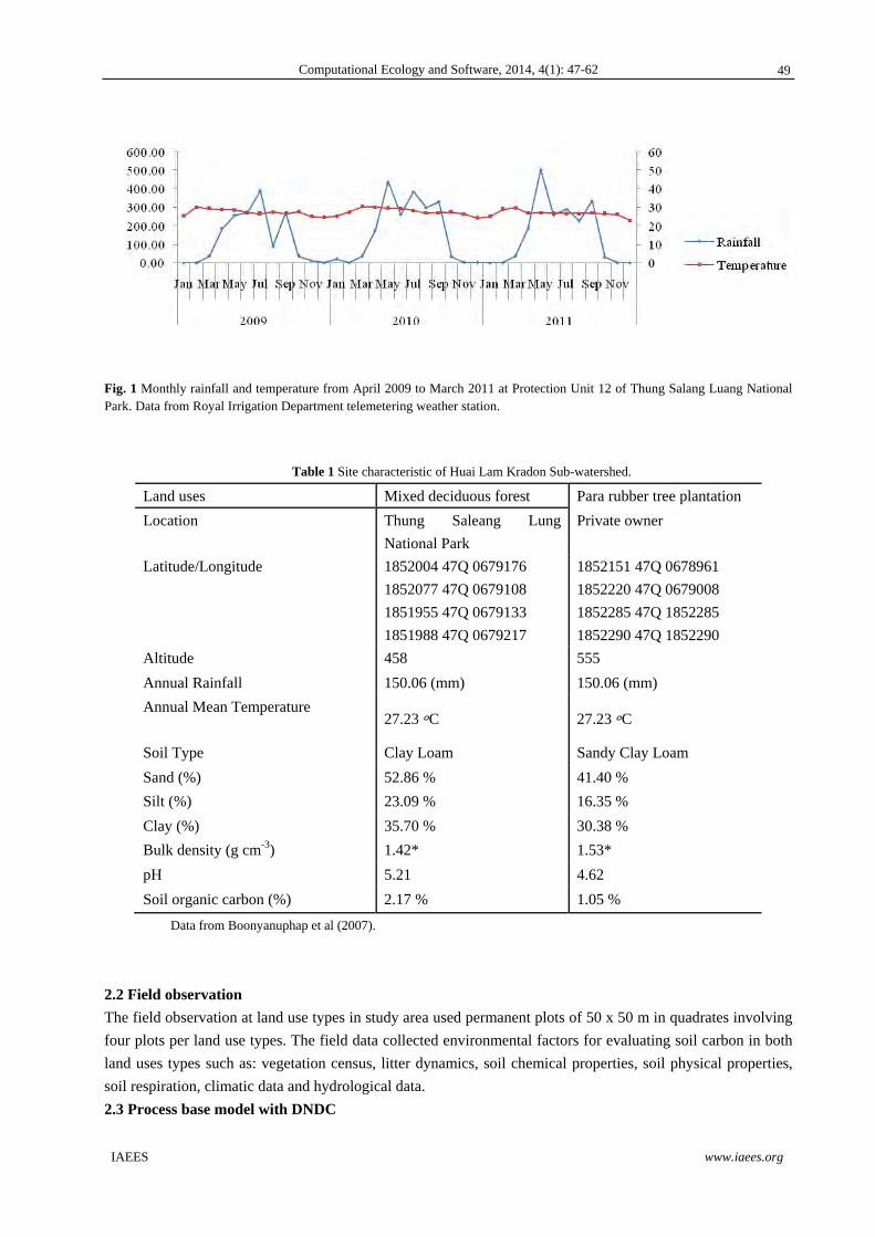
Computational Ecology and Software, 2014, 4(1): 47-62
IAEES www.iaees.org
Fig. 1 Monthly rainfall and temperature from April 2009 to March 2011 at Protection Unit 12 of Thung Salang Luang National Park. Data from Royal Irrigation Department telemetering weather station.
Table 1 Site characteristic of Huai Lam Kradon Sub-watershed.
Land uses Mixed deciduous forest Para rubber tree plantation
Location Thung Saleang Lung
National Park
Private owner
Latitude/Longitude 1852004 47Q 0679176
1852077 47Q 0679108
1851955 47Q 0679133
1851988 47Q 0679217
1852151 47Q 0678961
1852220 47Q 0679008
1852285 47Q 1852285
1852290 47Q 1852290
Altitude 458 555
Annual Rainfall 150.06 (mm) 150.06 (mm)
Annual Mean Temperature 27.23 ๐C 27.23 ๐C
Soil Type Clay Loam Sandy Clay Loam
Sand (%) 52.86 % 41.40 %
Silt (%) 23.09 % 16.35 %
Clay (%) 35.70 % 30.38 %
Bulk density (g cm-3) 1.42* 1.53*
pH 5.21 4.62
Soil organic carbon (%) 2.17 % 1.05 %
Data from Boonyanuphap et al (2007).
2.2 Field observation
The field observation at land use types in study area used permanent plots of 50 x 50 m in quadrates involving
four plots per land use types. The field data collected environmental factors for evaluating soil carbon in both
land uses types such as: vegetation census, litter dynamics, soil chemical properties, soil physical properties,
soil respiration, climatic data and hydrological data.
2.3 Process base model with DNDC
49
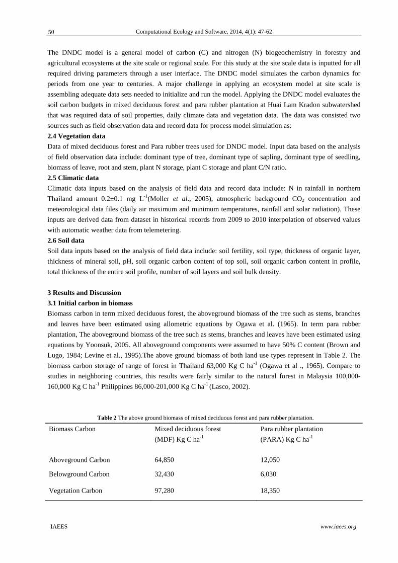
Computational Ecology and Software, 2014, 4(1): 47-62
IAEES www.iaees.org
The DNDC model is a general model of carbon (C) and nitrogen (N) biogeochemistry in forestry and
agricultural ecosystems at the site scale or regional scale. For this study at the site scale data is inputted for all
required driving parameters through a user interface. The DNDC model simulates the carbon dynamics for
periods from one year to centuries. A major challenge in applying an ecosystem model at site scale is
assembling adequate data sets needed to initialize and run the model. Applying the DNDC model evaluates the
soil carbon budgets in mixed deciduous forest and para rubber plantation at Huai Lam Kradon subwatershed
that was required data of soil properties, daily climate data and vegetation data. The data was consisted two
sources such as field observation data and record data for process model simulation as:
2.4 Vegetation data
Data of mixed deciduous forest and Para rubber trees used for DNDC model. Input data based on the analysis
of field observation data include: dominant type of tree, dominant type of sapling, dominant type of seedling,
biomass of leave, root and stem, plant N storage, plant C storage and plant C/N ratio.
2.5 Climatic data
Climatic data inputs based on the analysis of field data and record data include: N in rainfall in northern
Thailand amount 0.2±0.1 mg L-1(Moller et al., 2005), atmospheric background CO2 concentration and
meteorological data files (daily air maximum and minimum temperatures, rainfall and solar radiation). These
inputs are derived data from dataset in historical records from 2009 to 2010 interpolation of observed values
with automatic weather data from telemetering.
2.6 Soil data
Soil data inputs based on the analysis of field data include: soil fertility, soil type, thickness of organic layer,
thickness of mineral soil, pH, soil organic carbon content of top soil, soil organic carbon content in profile,
total thickness of the entire soil profile, number of soil layers and soil bulk density.
3 Results and Discussion
3.1 Initial carbon in biomass
Biomass carbon in term mixed deciduous forest, the aboveground biomass of the tree such as stems, branches
and leaves have been estimated using allometric equations by Ogawa et al. (1965). In term para rubber
plantation, The aboveground biomass of the tree such as stems, branches and leaves have been estimated using
equations by Yoonsuk, 2005. All aboveground components were assumed to have 50% C content (Brown and
Lugo, 1984; Levine et al., 1995).The above ground biomass of both land use types represent in Table 2. The
biomass carbon storage of range of forest in Thailand 63,000 Kg C ha-1 (Ogawa et al ., 1965). Compare to
studies in neighboring countries, this results were fairly similar to the natural forest in Malaysia 100,000-
160,000 Kg C ha-1 Philippines 86,000-201,000 Kg C ha-1 (Lasco, 2002).
Table 2 The above ground biomass of mixed deciduous forest and para rubber plantation.
Biomass Carbon Mixed deciduous forest
(MDF) Kg C ha-1
Para rubber plantation
(PARA) Kg C ha-1
Aboveground Carbon 64,850 12,050
Belowground Carbon 32,430 6,030
Vegetation Carbon 97,280 18,350
50
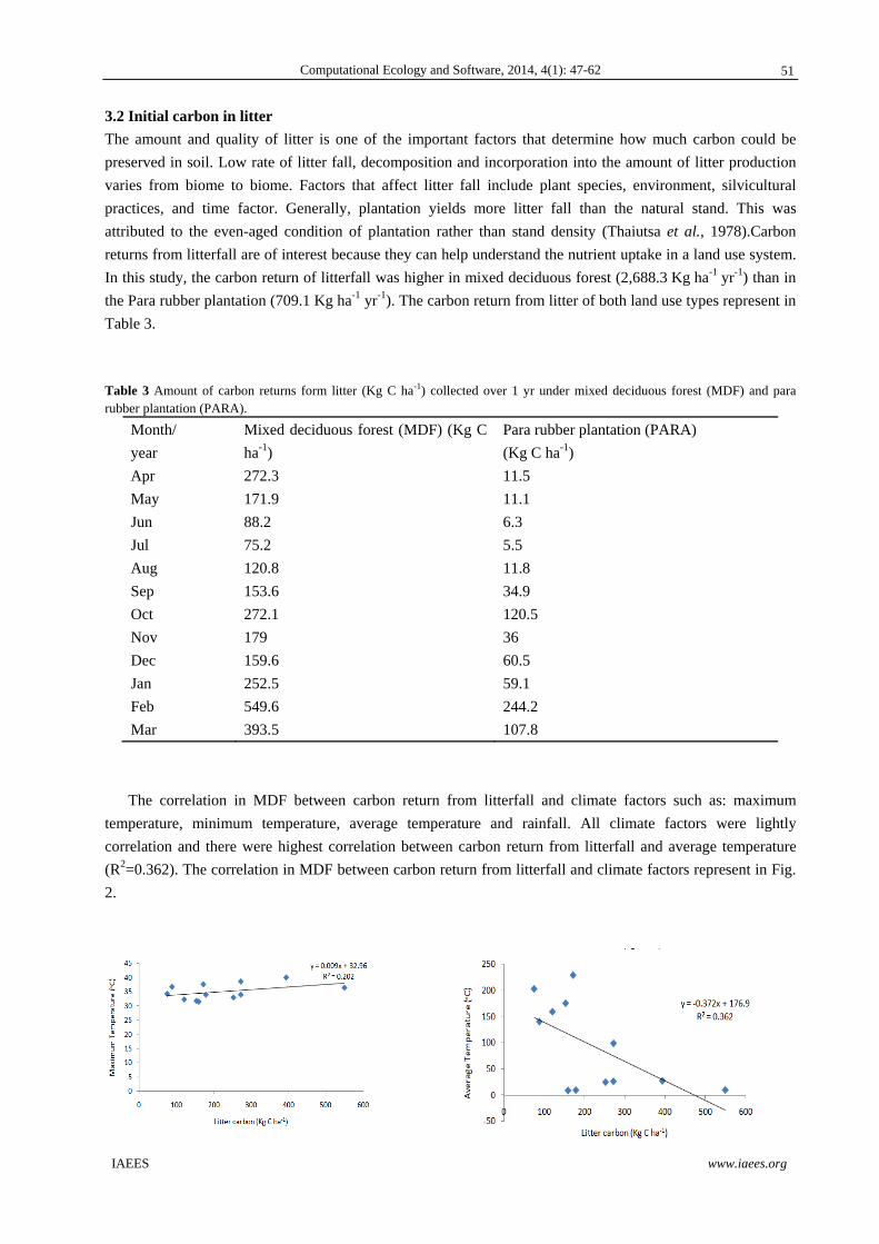
Computational Ecology and Software, 2014, 4(1): 47-62
IAEES www.iaees.org
3.2 Initial carbon in litter
The amount and quality of litter is one of the important factors that determine how much carbon could be
preserved in soil. Low rate of litter fall, decomposition and incorporation into the amount of litter production
varies from biome to biome. Factors that affect litter fall include plant species, environment, silvicultural
practices, and time factor. Generally, plantation yields more litter fall than the natural stand. This was
attributed to the even-aged condition of plantation rather than stand density (Thaiutsa et al., 1978).Carbon
returns from litterfall are of interest because they can help understand the nutrient uptake in a land use system.
In this study, the carbon return of litterfall was higher in mixed deciduous forest (2,688.3 Kg ha-1 yr-1) than in
the Para rubber plantation (709.1 Kg ha-1 yr-1). The carbon return from litter of both land use types represent in
Table 3.
Table 3 Amount of carbon returns form litter (Kg C ha-1) collected over 1 yr under mixed deciduous forest (MDF) and para rubber plantation (PARA).
Month/
year
Mixed deciduous forest (MDF) (Kg C
ha-1)
Para rubber plantation (PARA)
(Kg C ha-1)
Apr 272.3 11.5
May 171.9 11.1
Jun 88.2 6.3
Jul 75.2 5.5
Aug 120.8 11.8
Sep 153.6 34.9
Oct 272.1 120.5
Nov 179 36
Dec 159.6 60.5
Jan 252.5 59.1
Feb 549.6 244.2
Mar 393.5 107.8
The correlation in MDF between carbon return from litterfall and climate factors such as: maximum
temperature, minimum temperature, average temperature and rainfall. All climate factors were lightly
correlation and there were highest correlation between carbon return from litterfall and average temperature
(R2=0.362). The correlation in MDF between carbon return from litterfall and climate factors represent in Fig.
2.
51
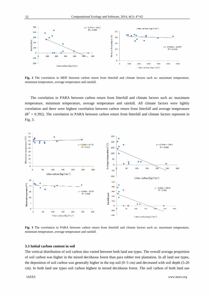
Computational Ecology and Software, 2014, 4(1): 47-62
IAEES www.iaees.org
Fig. 2 The correlation in MDF between carbon return from litterfall and climate factors such as: maximum temperature, minimum temperature, average temperature and rainfall.
The correlation in PARA between carbon return from litterfall and climate factors such as: maximum
temperature, minimum temperature, average temperature and rainfall. All climate factors were lightly
correlation and there were highest correlation between carbon return from litterfall and average temperature
(R2 = 0.392). The correlation in PARA between carbon return from litterfall and climate factors represent in
Fig. 3.
Fig. 3 The correlation in PARA between carbon return from litterfall and climate factors such as: maximum temperature, minimum temperature, average temperature and rainfall.
3.3 Initial carbon content in soil
The vertical distribution of soil carbon also varied between both land use types. The overall average proportion
of soil carbon was higher in the mixed deciduous forest than para rubber tree plantation. In all land use types,
the deposition of soil carbon was generally higher in the top soil (0–5 cm) and decreased with soil depth (5-20
cm). In both land use types soil carbon highest in mixed deciduous forest. The soil carbon of both land use
52
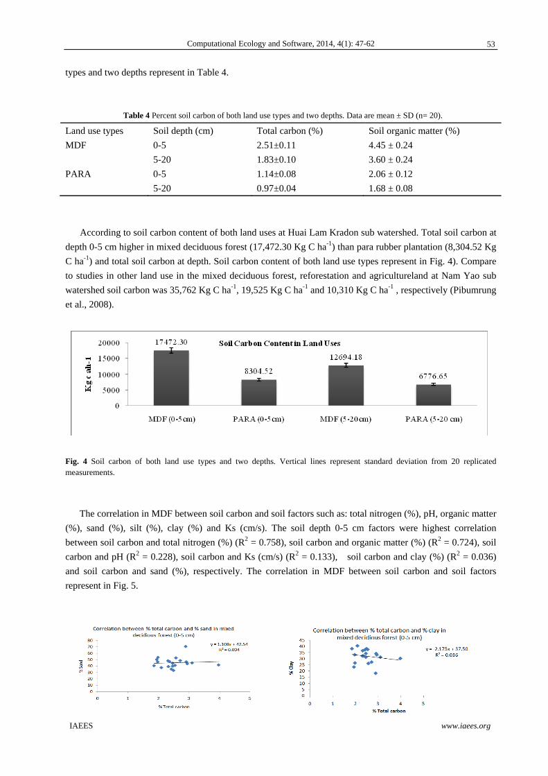
Computational Ecology and Software, 2014, 4(1): 47-62
IAEES www.iaees.org
types and two depths represent in Table 4.
Table 4 Percent soil carbon of both land use types and two depths. Data are mean ± SD (n= 20).
Land use types Soil depth (cm) Total carbon (%) Soil organic matter (%)
MDF 0-5 2.51±0.11 4.45 ± 0.24
5-20 1.83±0.10 3.60 ± 0.24
PARA 0-5 1.14±0.08 2.06 ± 0.12
5-20 0.97±0.04 1.68 ± 0.08
According to soil carbon content of both land uses at Huai Lam Kradon sub watershed. Total soil carbon at
depth 0-5 cm higher in mixed deciduous forest (17,472.30 Kg C ha-1) than para rubber plantation (8,304.52 Kg
C ha-1) and total soil carbon at depth. Soil carbon content of both land use types represent in Fig. 4). Compare
to studies in other land use in the mixed deciduous forest, reforestation and agricultureland at Nam Yao sub
watershed soil carbon was 35,762 Kg C ha-1, 19,525 Kg C ha-1 and 10,310 Kg C ha-1 , respectively (Pibumrung
et al., 2008).
Fig. 4 Soil carbon of both land use types and two depths. Vertical lines represent standard deviation from 20 replicated measurements.
The correlation in MDF between soil carbon and soil factors such as: total nitrogen (%), pH, organic matter
(%), sand (%), silt (%), clay (%) and Ks (cm/s). The soil depth 0-5 cm factors were highest correlation
between soil carbon and total nitrogen (%) (R2 = 0.758), soil carbon and organic matter (%) (R2 = 0.724), soil
carbon and pH (R2 = 0.228), soil carbon and Ks (cm/s) (R2 = 0.133), soil carbon and clay (%) (R2 = 0.036)
and soil carbon and sand (%), respectively. The correlation in MDF between soil carbon and soil factors
represent in Fig. 5.
53
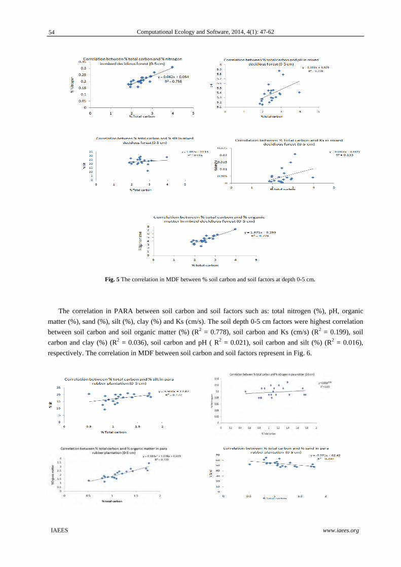
Computational Ecology and Software, 2014, 4(1): 47-62
IAEES www.iaees.org
Fig. 5 The correlation in MDF between % soil carbon and soil factors at depth 0-5 cm.
The correlation in PARA between soil carbon and soil factors such as: total nitrogen (%), pH, organic
matter (%), sand (%), silt (%), clay (%) and Ks (cm/s). The soil depth 0-5 cm factors were highest correlation
between soil carbon and soil organic matter (%) (R2 = 0.778), soil carbon and Ks (cm/s) (R2 = 0.199), soil
carbon and clay (%) (R2 = 0.036), soil carbon and pH ( R2 = 0.021), soil carbon and silt (%) (R2 = 0.016),
respectively. The correlation in MDF between soil carbon and soil factors represent in Fig. 6.
54
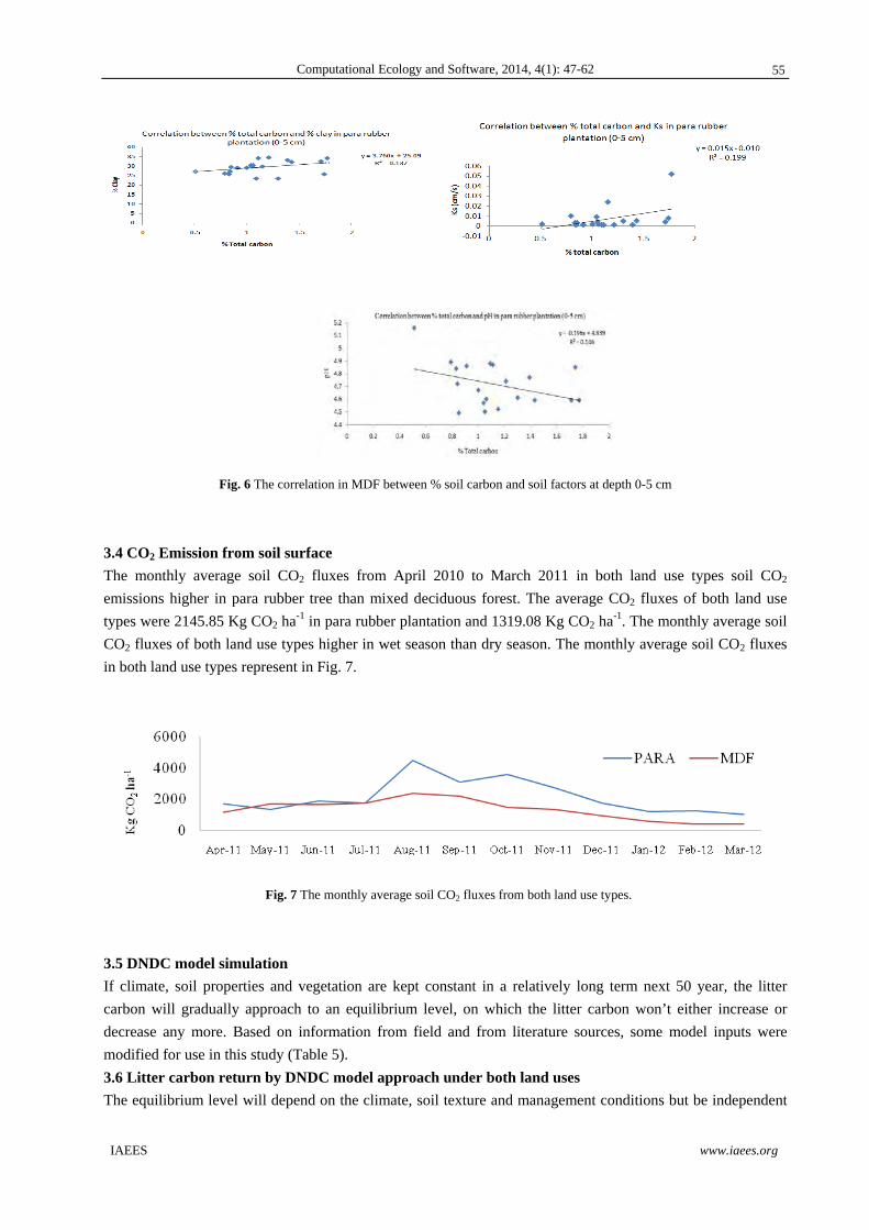
Computational Ecology and Software, 2014, 4(1): 47-62
IAEES www.iaees.org
Fig. 6 The correlation in MDF between % soil carbon and soil factors at depth 0-5 cm
3.4 CO2 Emission from soil surface
The monthly average soil CO2 fluxes from April 2010 to March 2011 in both land use types soil CO2
emissions higher in para rubber tree than mixed deciduous forest. The average CO2 fluxes of both land use
types were 2145.85 Kg CO2 ha-1 in para rubber plantation and 1319.08 Kg CO2 ha-1. The monthly average soil
CO2 fluxes of both land use types higher in wet season than dry season. The monthly average soil CO2 fluxes
in both land use types represent in Fig. 7.
Fig. 7 The monthly average soil CO2 fluxes from both land use types.
3.5 DNDC model simulation
If climate, soil properties and vegetation are kept constant in a relatively long term next 50 year, the litter
carbon will gradually approach to an equilibrium level, on which the litter carbon won’t either increase or
decrease any more. Based on information from field and from literature sources, some model inputs were
modified for use in this study (Table 5).
3.6 Litter carbon return by DNDC model approach under both land uses
The equilibrium level will depend on the climate, soil texture and management conditions but be independent
55
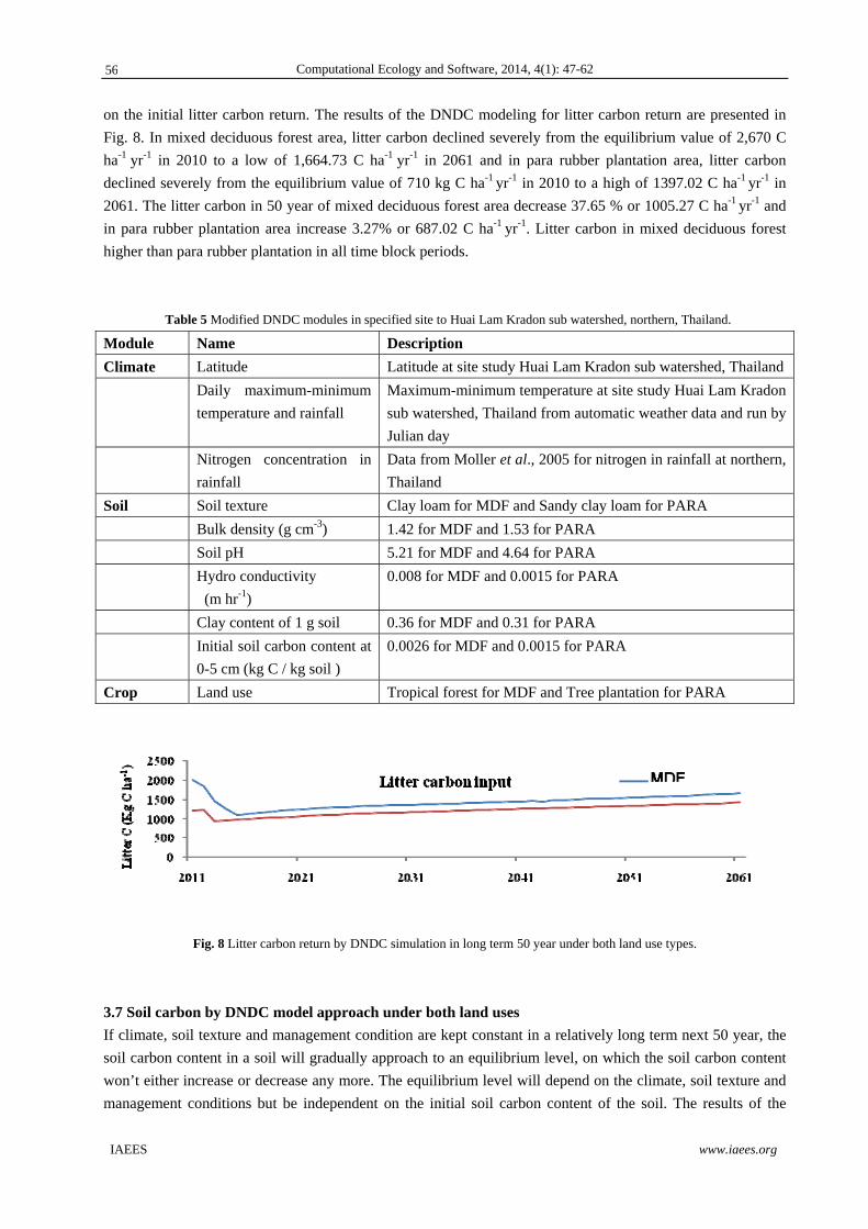
Computational Ecology and Software, 2014, 4(1): 47-62
IAEES www.iaees.org
on the initial litter carbon return. The results of the DNDC modeling for litter carbon return are presented in
Fig. 8. In mixed deciduous forest area, litter carbon declined severely from the equilibrium value of 2,670 C
ha-1 yr-1 in 2010 to a low of 1,664.73 C ha-1 yr-1 in 2061 and in para rubber plantation area, litter carbon
declined severely from the equilibrium value of 710 kg C ha-1 yr-1 in 2010 to a high of 1397.02 C ha-1 yr-1 in
2061. The litter carbon in 50 year of mixed deciduous forest area decrease 37.65 % or 1005.27 C ha-1 yr-1 and
in para rubber plantation area increase 3.27% or 687.02 C ha-1 yr-1. Litter carbon in mixed deciduous forest
higher than para rubber plantation in all time block periods.
Table 5 Modified DNDC modules in specified site to Huai Lam Kradon sub watershed, northern, Thailand.
Module Name Description
Climate Latitude Latitude at site study Huai Lam Kradon sub watershed, Thailand
Daily maximum-minimum
temperature and rainfall
Maximum-minimum temperature at site study Huai Lam Kradon
sub watershed, Thailand from automatic weather data and run by
Julian day
Nitrogen concentration in
rainfall
Data from Moller et al., 2005 for nitrogen in rainfall at northern,
Thailand
Soil Soil texture Clay loam for MDF and Sandy clay loam for PARA
Bulk density (g cm-3) 1.42 for MDF and 1.53 for PARA
Soil pH 5.21 for MDF and 4.64 for PARA
Hydro conductivity
(m hr-1)
0.008 for MDF and 0.0015 for PARA
Clay content of 1 g soil 0.36 for MDF and 0.31 for PARA
Initial soil carbon content at
0-5 cm (kg C / kg soil )
0.0026 for MDF and 0.0015 for PARA
Crop Land use Tropical forest for MDF and Tree plantation for PARA
Fig. 8 Litter carbon return by DNDC simulation in long term 50 year under both land use types.
3.7 Soil carbon by DNDC model approach under both land uses
If climate, soil texture and management condition are kept constant in a relatively long term next 50 year, the
soil carbon content in a soil will gradually approach to an equilibrium level, on which the soil carbon content
won’t either increase or decrease any more. The equilibrium level will depend on the climate, soil texture and
management conditions but be independent on the initial soil carbon content of the soil. The results of the
56
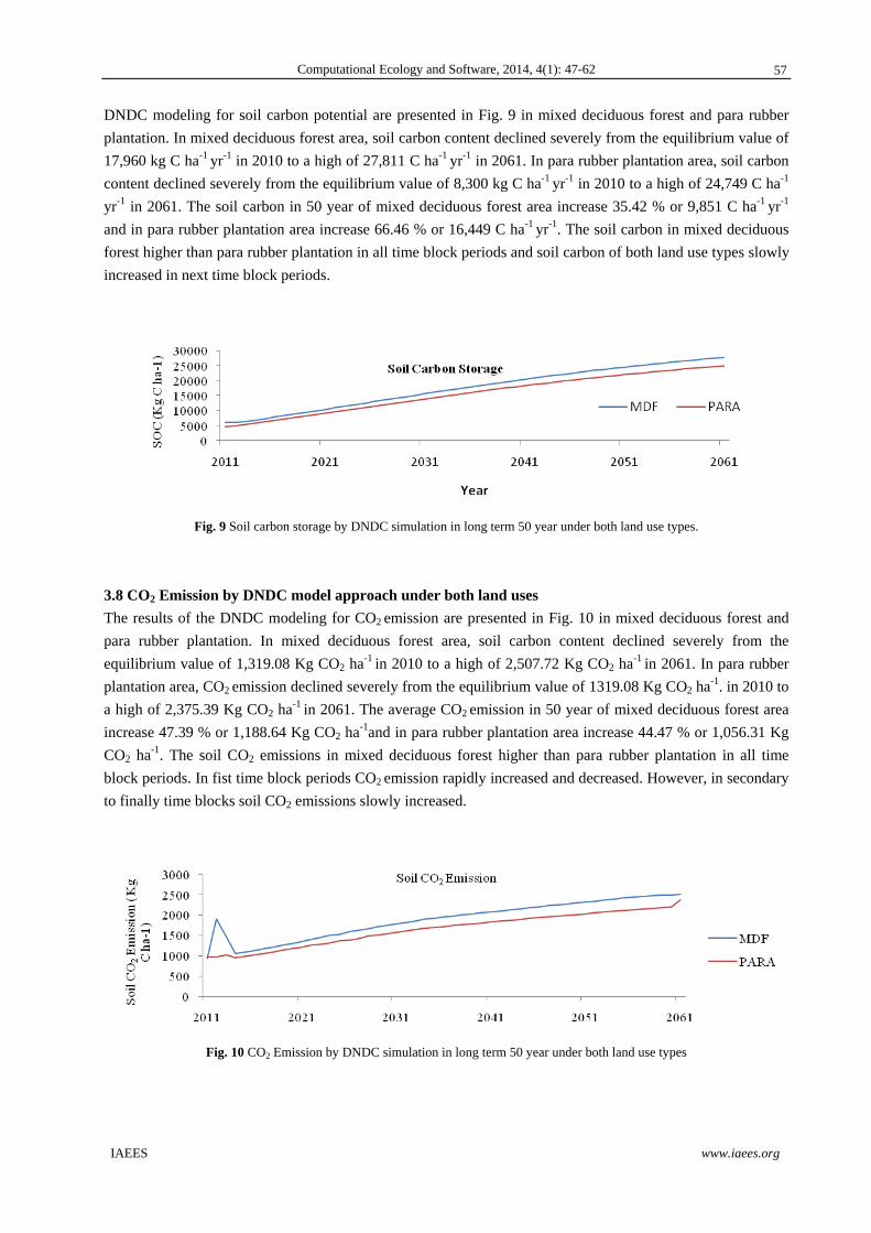
Computational Ecology and Software, 2014, 4(1): 47-62
IAEES www.iaees.org
DNDC modeling for soil carbon potential are presented in Fig. 9 in mixed deciduous forest and para rubber
plantation. In mixed deciduous forest area, soil carbon content declined severely from the equilibrium value of
17,960 kg C ha-1 yr-1 in 2010 to a high of 27,811 C ha-1 yr-1 in 2061. In para rubber plantation area, soil carbon
content declined severely from the equilibrium value of 8,300 kg C ha-1 yr-1 in 2010 to a high of 24,749 C ha-1
yr-1 in 2061. The soil carbon in 50 year of mixed deciduous forest area increase 35.42 % or 9,851 C ha-1 yr-1
and in para rubber plantation area increase 66.46 % or 16,449 C ha-1 yr-1. The soil carbon in mixed deciduous
forest higher than para rubber plantation in all time block periods and soil carbon of both land use types slowly
increased in next time block periods.
Fig. 9 Soil carbon storage by DNDC simulation in long term 50 year under both land use types.
3.8 CO2 Emission by DNDC model approach under both land uses
The results of the DNDC modeling for CO2 emission are presented in Fig. 10 in mixed deciduous forest and
para rubber plantation. In mixed deciduous forest area, soil carbon content declined severely from the
equilibrium value of 1,319.08 Kg CO2 ha-1 in 2010 to a high of 2,507.72 Kg CO2 ha-1 in 2061. In para rubber
plantation area, CO2 emission declined severely from the equilibrium value of 1319.08 Kg CO2 ha-1. in 2010 to
a high of 2,375.39 Kg CO2 ha-1 in 2061. The average CO2 emission in 50 year of mixed deciduous forest area
increase 47.39 % or 1,188.64 Kg CO2 ha-1and in para rubber plantation area increase 44.47 % or 1,056.31 Kg
CO2 ha-1. The soil CO2 emissions in mixed deciduous forest higher than para rubber plantation in all time
block periods. In fist time block periods CO2 emission rapidly increased and decreased. However, in secondary
to finally time blocks soil CO2 emissions slowly increased.
Fig. 10 CO2 Emission by DNDC simulation in long term 50 year under both land use types
57
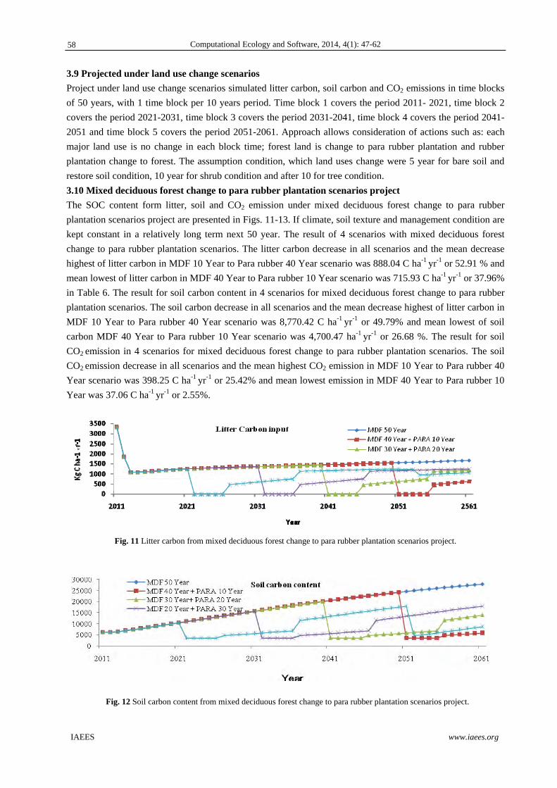
Computational Ecology and Software, 2014, 4(1): 47-62
IAEES www.iaees.org
3.9 Projected under land use change scenarios
Project under land use change scenarios simulated litter carbon, soil carbon and CO2 emissions in time blocks
of 50 years, with 1 time block per 10 years period. Time block 1 covers the period 2011- 2021, time block 2
covers the period 2021-2031, time block 3 covers the period 2031-2041, time block 4 covers the period 2041-
2051 and time block 5 covers the period 2051-2061. Approach allows consideration of actions such as: each
major land use is no change in each block time; forest land is change to para rubber plantation and rubber
plantation change to forest. The assumption condition, which land uses change were 5 year for bare soil and
restore soil condition, 10 year for shrub condition and after 10 for tree condition.
3.10 Mixed deciduous forest change to para rubber plantation scenarios project
The SOC content form litter, soil and CO2 emission under mixed deciduous forest change to para rubber
plantation scenarios project are presented in Figs. 11-13. If climate, soil texture and management condition are
kept constant in a relatively long term next 50 year. The result of 4 scenarios with mixed deciduous forest
change to para rubber plantation scenarios. The litter carbon decrease in all scenarios and the mean decrease
highest of litter carbon in MDF 10 Year to Para rubber 40 Year scenario was 888.04 C ha-1 yr-1 or 52.91 % and
mean lowest of litter carbon in MDF 40 Year to Para rubber 10 Year scenario was 715.93 C ha-1 yr-1 or 37.96%
in Table 6. The result for soil carbon content in 4 scenarios for mixed deciduous forest change to para rubber
plantation scenarios. The soil carbon decrease in all scenarios and the mean decrease highest of litter carbon in
MDF 10 Year to Para rubber 40 Year scenario was 8,770.42 C ha-1 yr-1 or 49.79% and mean lowest of soil
carbon MDF 40 Year to Para rubber 10 Year scenario was 4,700.47 ha-1 yr-1 or 26.68 %. The result for soil
CO2 emission in 4 scenarios for mixed deciduous forest change to para rubber plantation scenarios. The soil
CO2 emission decrease in all scenarios and the mean highest CO2 emission in MDF 10 Year to Para rubber 40
Year scenario was 398.25 C ha-1 yr-1 or 25.42% and mean lowest emission in MDF 40 Year to Para rubber 10
Year was 37.06 C ha-1 yr-1 or 2.55%.
Fig. 11 Litter carbon from mixed deciduous forest change to para rubber plantation scenarios project.
Fig. 12 Soil carbon content from mixed deciduous forest change to para rubber plantation scenarios project.
58
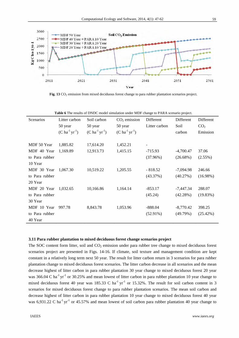
Computational Ecology and Software, 2014, 4(1): 47-62
IAEES www.iaees.org
Fig. 13 CO2 emission from mixed deciduous forest change to para rubber plantation scenarios project.
Table 6 The results of DNDC model simulation under MDF change to PARA scenario project.
Scenarios Litter carbon
50 year
(C ha-1 yr-1)
Soil carbon
50 year
(C ha-1 yr-1)
CO2 emission
50 year
(C ha-1 yr-1)
Different
Litter carbon
Different
Soil
carbon
Different
CO2
Emission
MDF 50 Year 1,885.82 17,614.20 1,452.21 -
MDF 40 Year
to Para rubber
10 Year
1,169.89 12,913.73
1,415.15 -715.93
(37.96%)
-4,700.47
(26.68%)
37.06
(2.55%)
MDF 30 Year
to Para rubber
20 Year
1,067.30
10,519.22
1,205.55 - 818.52
(43.37%)
-7,094.98
(40.27%)
246.66
(16.98%)
MDF 20 Year
to Para rubber
30 Year
1,032.65 10,166.86
1,164.14 -853.17
(45.24)
-7,447.34
(42.28%)
288.07
(19.83%)
MDF 10 Year
to Para rubber
40 Year
997.78 8,843.78 1,053.96 -888.04
(52.91%)
-8,770.42
(49.79%)
398.25
(25.42%)
3.11 Para rubber plantation to mixed deciduous forest change scenarios project
The SOC content form litter, soil and CO2 emission under para rubber tree change to mixed deciduous forest
scenarios project are presented in Figs. 14-16. If climate, soil texture and management condition are kept
constant in a relatively long term next 50 year. The result for litter carbon return in 3 scenarios for para rubber
plantation change to mixed deciduous forest scenarios. The litter carbon decrease in all scenarios and the mean
decrease highest of litter carbon in para rubber plantation 30 year change to mixed deciduous forest 20 year
was 366.04 C ha-1 yr-1 or 30.25% and mean lowest of litter carbon in para rubber plantation 10 year change to
mixed deciduous forest 40 year was 185.33 C ha-1 yr-1 or 15.32%. The result for soil carbon content in 3
scenarios for mixed deciduous forest change to para rubber plantation scenarios. The mean soil carbon and
decrease highest of litter carbon in para rubber plantation 10 year change to mixed deciduous forest 40 year
was 6,931.22 C ha-1 yr-1 or 45.57% and mean lowest of soil carbon para rubber plantation 40 year change to
59
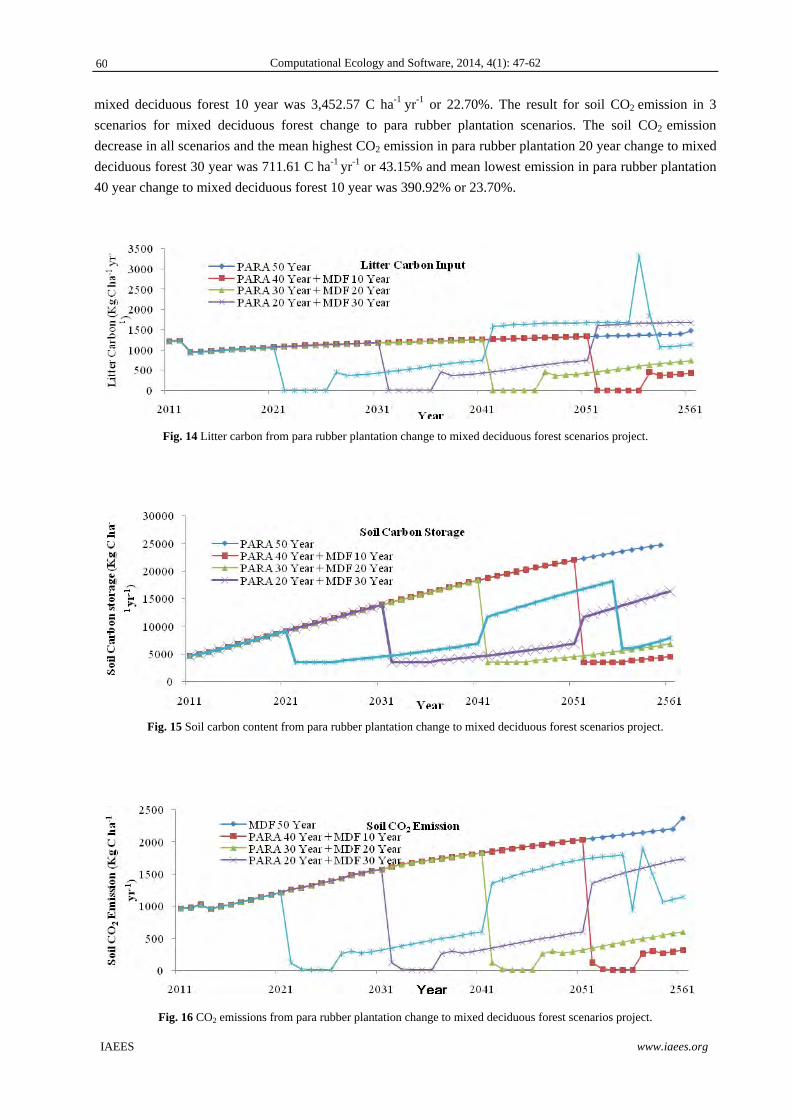
Computational Ecology and Software, 2014, 4(1): 47-62
IAEES www.iaees.org
mixed deciduous forest 10 year was 3,452.57 C ha-1 yr-1 or 22.70%. The result for soil CO2 emission in 3
scenarios for mixed deciduous forest change to para rubber plantation scenarios. The soil CO2 emission
decrease in all scenarios and the mean highest CO2 emission in para rubber plantation 20 year change to mixed
deciduous forest 30 year was 711.61 C ha-1 yr-1 or 43.15% and mean lowest emission in para rubber plantation
40 year change to mixed deciduous forest 10 year was 390.92% or 23.70%.
Fig. 14 Litter carbon from para rubber plantation change to mixed deciduous forest scenarios project.
Fig. 15 Soil carbon content from para rubber plantation change to mixed deciduous forest scenarios project.
Fig. 16 CO2 emissions from para rubber plantation change to mixed deciduous forest scenarios project.
60
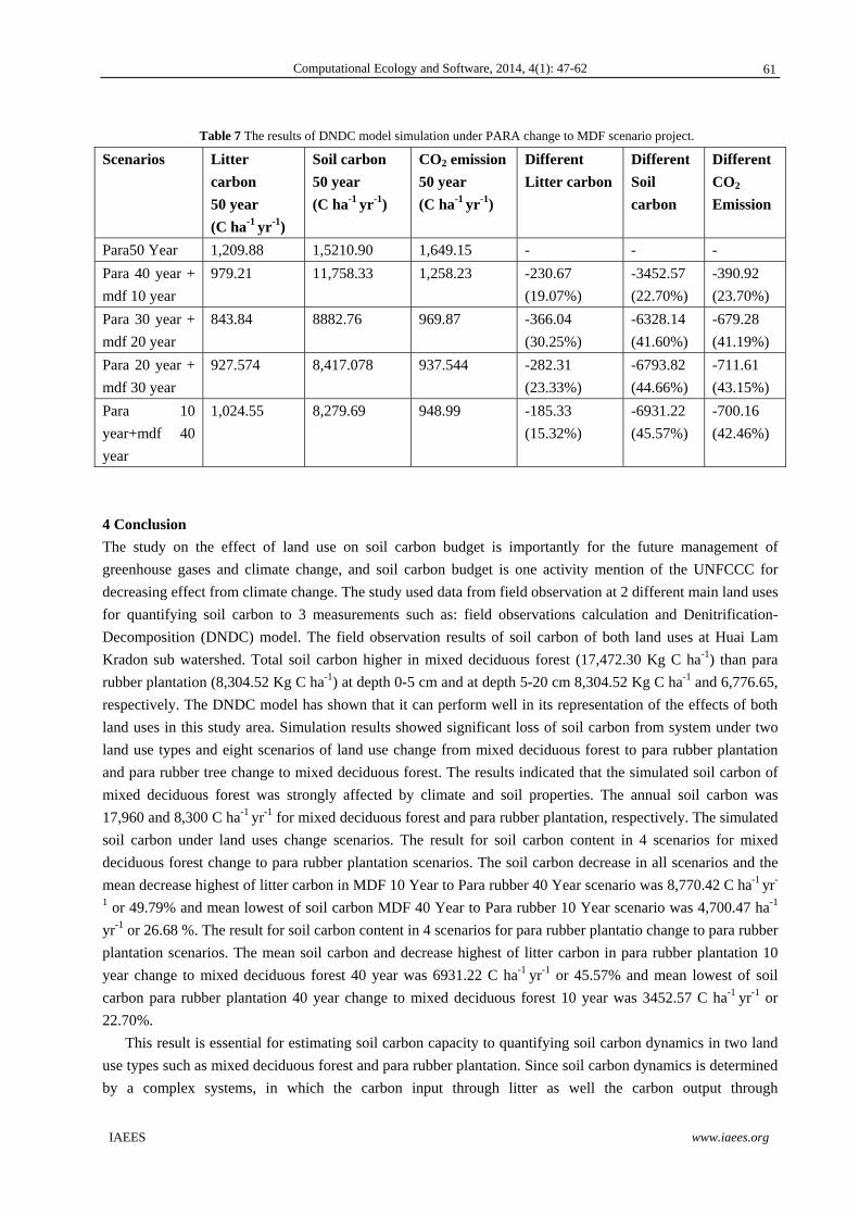
Computational Ecology and Software, 2014, 4(1): 47-62
IAEES www.iaees.org
Table 7 The results of DNDC model simulation under PARA change to MDF scenario project.
Scenarios Litter
carbon
50 year
(C ha-1 yr-1)
Soil carbon
50 year
(C ha-1 yr-1)
CO2 emission
50 year
(C ha-1 yr-1)
Different
Litter carbon
Different
Soil
carbon
Different
CO2
Emission
Para50 Year 1,209.88 1,5210.90 1,649.15 - - -
Para 40 year +
mdf 10 year
979.21
11,758.33
1,258.23
-230.67
(19.07%)
-3452.57
(22.70%)
-390.92
(23.70%)
Para 30 year +
mdf 20 year
843.84
8882.76
969.87
-366.04
(30.25%)
-6328.14
(41.60%)
-679.28
(41.19%)
Para 20 year +
mdf 30 year
927.574
8,417.078
937.544
-282.31
(23.33%)
-6793.82
(44.66%)
-711.61
(43.15%)
Para 10
year+mdf 40
year
1,024.55
8,279.69
948.99
-185.33
(15.32%)
-6931.22
(45.57%)
-700.16
(42.46%)
4 Conclusion
The study on the effect of land use on soil carbon budget is importantly for the future management of
greenhouse gases and climate change, and soil carbon budget is one activity mention of the UNFCCC for
decreasing effect from climate change. The study used data from field observation at 2 different main land uses
for quantifying soil carbon to 3 measurements such as: field observations calculation and Denitrification-
Decomposition (DNDC) model. The field observation results of soil carbon of both land uses at Huai Lam
Kradon sub watershed. Total soil carbon higher in mixed deciduous forest (17,472.30 Kg C ha-1) than para
rubber plantation (8,304.52 Kg C ha-1) at depth 0-5 cm and at depth 5-20 cm 8,304.52 Kg C ha-1 and 6,776.65,
respectively. The DNDC model has shown that it can perform well in its representation of the effects of both
land uses in this study area. Simulation results showed significant loss of soil carbon from system under two
land use types and eight scenarios of land use change from mixed deciduous forest to para rubber plantation
and para rubber tree change to mixed deciduous forest. The results indicated that the simulated soil carbon of
mixed deciduous forest was strongly affected by climate and soil properties. The annual soil carbon was
17,960 and 8,300 C ha-1 yr-1 for mixed deciduous forest and para rubber plantation, respectively. The simulated
soil carbon under land uses change scenarios. The result for soil carbon content in 4 scenarios for mixed
deciduous forest change to para rubber plantation scenarios. The soil carbon decrease in all scenarios and the
mean decrease highest of litter carbon in MDF 10 Year to Para rubber 40 Year scenario was 8,770.42 C ha-1 yr-
1 or 49.79% and mean lowest of soil carbon MDF 40 Year to Para rubber 10 Year scenario was 4,700.47 ha-1
yr-1 or 26.68 %. The result for soil carbon content in 4 scenarios for para rubber plantatio change to para rubber
plantation scenarios. The mean soil carbon and decrease highest of litter carbon in para rubber plantation 10
year change to mixed deciduous forest 40 year was 6931.22 C ha-1 yr-1 or 45.57% and mean lowest of soil
carbon para rubber plantation 40 year change to mixed deciduous forest 10 year was 3452.57 C ha-1 yr-1 or
22.70%.
This result is essential for estimating soil carbon capacity to quantifying soil carbon dynamics in two land
use types such as mixed deciduous forest and para rubber plantation. Since soil carbon dynamics is determined
by a complex systems, in which the carbon input through litter as well the carbon output through
61
Computational Ecology and Software, 2014, 4(1): 47-62
IAEES www.iaees.org
decomposition are collectively and simultaneously controlled by a pattern of natural and management factors
(Li et al., 1994). In Thailand, especially in Northern Thailand, soil carbon loss from land used change from
forest to agriculture land. The model results indicated that soil carbon sequestration potential can be
substantially elevated if the people protected forest area before change and manage agriculture are after change
because from the model result soil carbon dynamics in both land use little different in long time 50 year.
Acknowledgement
The research was supported by a CHE-Ph.D-SW-NEWU scholarship from the Commission on Higher
Education. The Department of National Parks, Wildlife and Plant Conservation is thanked for giving
permission to access and collect data from the study area.
References
Bajracharya RM, Lal R, Kimble JM. 1998. Long-term tillage effect on soil organic carbon distribution in
aggregate and primary particle fractions of two Ohio soils. In: Management of Carbon Sequestration in
Soil (Lal R, Kimble JM, Follett RF, et al., eds). 113-123, CRC Press, Boca Raton, USA
Boonyanuphap J, Sakurai K, Tanaka S. 2007. Soil nutrient status under upland farming practice in the Lower
Northern Thailand. Tropics, 16(3): 215-231
Brown S, Lugo AE. 1984. Biomass of tropical forests: A new estimate based on forest volumes. Science, 223:
1290-1293
Lasco RD. 2002. Forest carbon budgets in Southeast Asia following harvesting and land cover change. Science
in China (Series C), 45: 55-64
Levine JS. 1995. Biomass burning, a driver for global change. Environmental Science and Technology Letters,
120: 120-125
Li C, Frolking SF, Harriss RC. 1994. Modeling carbon biogeochemistry in agriculture soils. Global
Biogeochemical Cycles, 8: 237-254
Moller A, Kaiser K, Guggenberger G. 2005. Dissolved organic carbon and nitrogen in precipitation,
through fall, soil solution, and stream water of the tropical highlands in northern Thailand. Journal of Plant
Nutrition and Soil Science, 168: 649-659
Ogawa H, Yoda K, Ogino K, et al. 1965. Comparative ecological studies on three main types of forest
vegetation in Thailand II. Plant Biomass. Nature and Life in Southeast Asia, 4: 49-80
Pibumrung P, Gajaseni N, Popan A. 2008. Profiles of carbon stocks in forest, reforestation and agricultural
land, Northern Thailand. Journal of Forest Research, 19: 11-18
Tan ZX, Lal R, Izaurralde RC, et al. 2004. Biochemically protected soil organic carbon at the Appalachian
experimental watershed. Soil Science, 169(6): 423-433
Thaiutsa B, Suwannapinunt W, Kaitpraneet W. 1978. Production and Chemical Composition of Forest Litter
in Thailand. Forest Research Bulletin. Kasetsart University, Bangkok, Thailand
Yoosuk S. 2005. Carbon Sink in Rubber Plantation of Klaeng District, Rayong Province. MSc Thesis, Mahidol
University, Thailand
Zhang WJ, Qi YH, Zhang ZG. 2006. A long-term forecast analysis on worldwide land uses. Environmental
Monitoring and Assessment, 119: 609-620
Zhang Y, Li CS, Zhou X, et al. 2002. A simulation model linking crop growth and soil biogeochemistry for
sustainable agriculture. Ecological Modelling, 151: 75-108
62

Computational Ecology and Software, 2014, 4(1): 63-81
IAEES www.iaees.org
Article
Analytical treatment of system of KdV equations by Homotopy
Perturbation Method (HPM) and Homotopy Analysis Method (HAM)
Hafiz Abdul Wahab1, Tahir Khan1, Muhammad Shakil1, Saira Bhatti2, Muhammad Naeem3 1Department of Mathematics, Hazara University, Mansehra, Pakistan 2Department of Mathematics, COMSATS Institute of Information Technology, Abbottabad, Pakistan 3Department of Information Technology, Hazara University, Mansehra, Pakistan
E-mail: [email protected]
Received 16 September 2013; Accepted 20 October 2013; Published online 1 March 2014
Abstract
In this article the Homotopy Perturbation Method (HPM) and Homotopy Analysis Method (HAM) are applied
to obtain analytic approximate solution to three system of nonlinear wave equations, namely two component
evolutionary system of a homogeneous KdV Equations of order three (system-I) as well as (system-II) and the
generalized coupled Hirota Satsuma KdV (System-III).
Keywords Homotopy Perturbation Method (HPM); Homotopy Analysis Method (HAM); Systems of KdV
equations.
1 Introduction
In different field the nonlinear phenomena is very important and it played a tremendous role, especially in the
field of applied mathematics, engineering and physics etc. Now for mechanism of physical model described by
differential equations, different types of effective methods have been discovered for helping the engineers,
scientist and physicist to know about the problem and its application, because in most cases it is still difficult
to obtain the exact solution.
Like other nonlinear analytic technique Homotopy Perturbation Method (HPM) and Homotopy Analysis
Method (HAM) are two well known methods for obtaining the analytic approximate solutions to differential
equations. In He (1999), the Homotopy Perturbation Method (HPM) was first presented. The Homotopy
Perturbation Method (HPM) applied by many authors (Shakil et al, 2013; Siddiqui et al., 2014; Wahab et al.,
2013; Wahab et al., 2014), to find the solution of nonlinear problems in the field of science and engineering.
This method have the ability to solve linear and nonlinear problems (Alquran and Muhammad, 2011; Hemeda,
2012). Homotopy Perturbation Method (HPM) provides an opportunity that is no requirement of small
parameter like perturbation methods, in the equations. Homotopy Perturbation Method (HPM) also applicable
Computational Ecology and Software ISSN 2220721X URL: http://www.iaees.org/publications/journals/ces/onlineversion.asp RSS: http://www.iaees.org/publications/journals/ces/rss.xml Email: [email protected] EditorinChief: WenJun Zhang Publisher: International Academy of Ecology and Environmental Sciences
Computational Ecology and Software, 2014, 4(1): 63-81
IAEES www.iaees.org
to different types of equations like Volterra’s equation, integro equation, nonlinear oscillator equation,
bifurcation equation, nonlinear wave equation etc (Hemeda, 2012). In most cases Homotopy Perturbation
Method (HPM) provides a very rapid and fast convergence (Hemeda, 2012). Thus a method which have the
ability to solve different types of nonlinear equations is known as Homotopy Perturbation Method (HPM).
Liao has presented another analytic approximation in 1992 (Liao, 1992). This method is based on a
interesting property called homotopy, a fundamental concept of differential geometry and topology (Taiwo et
al., 2012). Homotopy Analysis Method (HAM) is an analytic approximated method through which we can find
the solution of nonlinear problem. Since perturbation techniques are often non valid in case of strong non
linearity, but Homotopy Analysis Method (HAM) is valid in non-linearity case (Liao, 2003). By using one
interesting property of homotopy, the non-linear problem can be changed into an infinite number of linear
problems, no matter comes from small or large parameter. If a non-linear problem has even a single solution,
then through this method namely Homotopy Analysis Method (HAM), there exist an infinite number of
disjoint solution expression whose the region of convergence and rate of convergence dependent on an axillary
parameter (Liao, 2003).
The purpose of this paper is to present analytic approximate solution to system of KdV equations by using
Homotopy Perturbation Method (HPM) and Homotopy Analysis Method (HAM).
2 Analysis of Homotopy Perturbation Method (HPM)
Let us consider a general nonlinear differential equation of the form,
,L x x g z z (1)
subject to the boundary condition,
, 0,x
x zn
(2)
In equation (1)-(2), " "L is the linear operator. " "N is the nonlinear operator. " " is defined to be the
boundary operator. Boundary of the domain " " is " " . The known function is define to be the function
" "g z . Now by Homotopy Analysis Method (HAM) constructing a homotopy, such that,
, : [0,1]r q R ,
which satisfies,
0, 1 ( ) ( ) 0H L L x L g z (3)
Equation (3), becomes
0 0, 0H L L x L x N g z (4)
where " "z and " 0,1 " is known to be the embedding parameter, 0" "x is define to be the, so
called initial approximation, must satisfies the boundary condition. Now setting " 0" and " 1" in
equation (4), then
0,0 0H L L x (5)
,1 0H L g z (6)
Equation (5) and equation (6), are called homotopic equations and the value of " " changing from
64
Computational Ecology and Software, 2014, 4(1): 63-81
IAEES www.iaees.org
"0" to unity is called deformation in topology (Hemeda, 2012). Now according to Homotopy Perturbation
Method (HPM), the basic assumption of the for the solution of equation (3)-(4) the basic assumption is that,
the " " can be expressed in a power series, such that,
0 1, ; , , ...x t v x t v x t (7)
and thus the analytical approximate solution for equation (1), can be derived through Homotopy Perturbation
Method (HPM) by setting " 1" in equation (7), which becomes,
0 1 21lim , ; ...q
x x t v v v
(8)
which will be the required approximated solution of the given nonlinear problem derived by Homotopy
Perturbation Method (HPM).
3 Analysis of Homotopy Analysis Method (HAM)
Homotopy Analysis Method (HAM) is a straight forward and very simple method. This method was presented
by means of homotopy (Hilton, 1953; Liao, 2003), which is a fundamental concept of topology.
Consider a differential equation, such that
, 0x t (9)
In equation (9), " " is non-linear operator and " , "x t is the unknown function. Now the
generalization of the traditional homotopy by Homotopy Perturbation Method (HPM) presented by Liao
(2003), construct a new type of homotopy called deformation equation of zero-order, such that,
01 , ; , , ( , ; )L x t x t x t x t (10)
In equation (10), 0" , "x t is known to be the initial approximation of the given unknown function that
is, " , "x t . " , ; "x t is a function, which is not known. " " is the embedding parameter, " "
and " , "H x t are the non-zero auxiliary parameter and non-zero auxiliary function respectively, " " is
the operator called non-linear and " "L is the auxiliary operator called linear operator. In this method it is
very important that we can easily and with great freedom chose the auxiliary materials (Hemeda, 2012).
Now if 0 and 1 , then equation (10), becomes,
0, ;0 ,x t x t and ( , ;1) ( , )x t x t (11)
Thus equation (11), shows that the variation of the embedding parameter varies from zero to unity make the
solution " , ; "x t from the initial approximation to the exact solution. The variation of these kind is
called deformation in the manner of topology (Liao, 2003).
According to Homotopy Analysis Method (HAM), expending " " in a power series with respect to
" " . Such that,
20 1 2
00
, ; ...
, ; mm
m
x t
x t
(12)
In equation (12), , ;" , "
!
m
m m
x tx t
m
at " 0" . Now if the auxiliary elements that is, the
65
Computational Ecology and Software, 2014, 4(1): 63-81
IAEES www.iaees.org
auxiliary linear-operator, auxiliary parameter, the initial-approximation and the auxiliary function are chosen
through proper way, then the above series that is series in equation (12), is convergent at " 1" . Thus the
solution of the original non-linear problem becomes,
01
mm
m
(13)
which is one-solution of the original nonlinear problem. Now according to the fundamental theorem of
Homotopy Analysis Method (HAM), consider a vector, such that,
0 1, ,..., n
(14)
Then the deformation equation of order " "m is given by
1 1. , .m m m m mL x t
(15)
In equation (15),
0, 1
1, 1m
m
m
and
1
1 1
, ;
1 !
m
m m m
x t
m
(16)
Now if " 1" and " , 1"H x t in equation (10), then it become homotopy constructed in
Homotopy Perturbation Method (HPM), which shows that Homotopy Perturbation Method (HPM) is a
specified case of Homotopy Analysis Method (HAM). The genialized homotopy only not depend on the
parameter " " , but it also dependent on" " and " , "x t called auxiliary parameter and auxiliary function
respectively. Thus the generalized homotopy give us a family of approximation series whose the region of
convergence depend upon on " " and " , "x t . Also the generalized homotopy provide us a straight
forward way to control and adjust the convergence region and rate of approximation series (Liao, 2003).
Homotopy Analysis Method (HAM) is more general and valid for non-linear and linear Differential equations
in many types.
This is a very brief introduction, for details, we refer to Liao (2003), Hemeda (2012), Zedan and El Adrous
(2012).
4 Applications
Taking the following systems of nonlinear KdV equations.
System-I
Consider the first system is a system of KdV equations of order three, such that
3
3,
t x x x
(17)
3
32 ,
t x x
(18)
subject to,
20 3 6 tanh ,
2
x
(19)
66
Computational Ecology and Software, 2014, 4(1): 63-81
IAEES www.iaees.org
1
220 3 2 tanh .
2
xi
(20)
The closed form solution given in Alquran and Muhammad (2011), is as,
23 6 tanh ,2closed
x t
23 2 tanh .2closed
x ti
Homotopy Perturbation Method (HPM) Solution
Through Homotopy Perturbation Method (HPM) the approximate solution of the system-I is derived as,
2 2 2 4
3 2
3 tanh 6 3 6 tanh tanh sec 24sec2 2 2 2 2
,
tanh 24 tanh sec ...2 2 2
HPM
x x x x xt h h
x tx x x
t h
2 4
2 3
9 2 sec tanh 24 2 sec tanh 12 22 2 2 2
,
sec tanh ...2 2
HPM
x x x xit h it h it
x tx x
h
Solution by Homotopy Analysis Method (HAM)
To solve system-I by Homotopy Analysis Method (HAM), and keeping in the view the given conditions, we
define a linear-operator as, " "Lt
and the inverse of linear operator is define as, 1
0
" () "t
L dt . Now
by definition of Homotopy Analysis Method (HAM), the deformation equation of order-zero for the given
system of non-linear partial differential equations becomes,
1 0 11 , ; . . , . , ; ,L x t x t x t (21)
2 0 21 , ; . . , . , ; ,L x t x t x t (22)
where 0 0" , " are the given initial approximation define as,
20 ,0 3 6 tanh ,
2
xx
(23)
1
220 ,0 3 2 tanh .
2
xx i
(24)
Now since " " is the embedding parameter, so the deformation process gives us,
1 0, ;0 ,x t (25)
67
Computational Ecology and Software, 2014, 4(1): 63-81
IAEES www.iaees.org
2 0, ;0 ,x t (26)
1 , ;1 ,x t (27)
2 , ;1 .x t (28)
Now suppose that, the solution of the original equation can be expressed in the power of the embedding
parameter, such that,
1 01
, ; ,nn
n
x t
(29)
2 01
, ; .nn
n
x t
(30)
In equation (29)-(30), 1 , ;1
!
n
n n
x t
n
and 2 , ;1
!
n
n n
x t
n
at " 0" and exist for
" 1"n also converges at " 1" . Then the solution of the given problem becomes,
01
,nn
(31)
01
.nn
(32)
Now the fundamental theorem of Homotopy Analysis Method (HAM) provide us, that the deformation
equation of nth-order for the given system of nonlinear PDEs becomes,
1 1, ,n n n n nL x t
(33)
1 1, .n n n n nL x t
(34)
Applying the inverse operator that is, 1
0
" . "t
L dt , on equation (33)-(34), we obtain,
1 1
0
, ,t
n n n n nx t dt
(35)
1 1
0
, .t
n n n n nx t dt
(36)
Starting with the initial approximation,
20 , 3 6 tanh ,2
xx t (37)
20 , 3 2 tanh .2
xx t i (38)
68
Computational Ecology and Software, 2014, 4(1): 63-81
IAEES www.iaees.org
Now substituting " 1"n and also for simplicity using " ( , ) 1"x t in equation (35)-(36), we get,
2 2 4
1
3 2
6 3 6 tanh tanh sec 24 sec2 2 2 2
, ,
tanh 24 tanh sec2 2 2
x x x xt h t h
x tx x x
t h
(39)
2 4
12 3
9 2 sec tanh 24 2 sec2 2 2
, .
tanh 12 2 sec tanh2 2 2
x x xi t h i t h
x tx x x
i t h
(40)
Similarly for obtaining 2 2 3 3, , , , and so on, using " 2,3, 4,..."n in equation (35)-(36). Now to
obtain the analytic approximate solution of the given system of KdV equation by Homotopy Analysis Method
(HAM), since
0 1 2, ( , ) ( , ) ( , ) ...x t x t x t x t (41)
0 1 2( , ) ( , ) ( , ) ( , ) ...x t x t x t x t (42)
Using the initial gauss, 1 1" , " and also the 2nd components that is 2 2" , " obtained through Maple
package given in appendix, in equation (41)-(42), we will get the solution by Homotopy Analysis Method
(HAM). After the derivation of the solution by Homotopy Analysis Method (HAM), if we use the non-zero
auxiliary parameter that is," 1" in the obtained solution by Homotopy Analysis Method (HAM), it will
give us the Homotopy Perturbation Method (HPM) solution, which shows that Homotopy Perturbation Method
(HPM) is a specified case of Homotopy Analysis Method (HAM).
System-II
In this system, we consider two component evolutionary system of KdV equation of order three, such that,
3
32 0,
t x x x
(43)
0,t x
(44)
initial condition,
0 1
2
tanh ,3
x
(45)
2
0 1
2
1 1tanh .
6 2 3
x
(46)
69
Computational Ecology and Software, 2014, 4(1): 63-81
IAEES www.iaees.org
The closed form solution given in Alquran and Muhammad (2011), that is
1
2
tanh ,3
closed
x t
2
1
2
1 1tanh .
6 2 3closed
x t
Homotopy Perturbation solution
The approximated analytic solution obtained by Homotopy Perturbation Method (HPM) is as,
2 2 21 1 1 1
2 2 2 2
2 2 41 1 1
2 2 2
tanh sec tanh sec3 3 33 3 3 3
2tanh sec sec ...
3 3 3 33 3 3
HPM
x t x t x xh h
t x x t xh h
(47)
2 2
1 1 1
2 2 2
1 1tanh tanh sec ...
6 2 33 3 3HPM
x t x xh
(48)
Solution by Homotopy Analysis Method
Now we want to find out the analytic approximated solution of the system-II, by Homotopy Analysis Method
(HAM), and then to compare it with the the result obtained by Homotopy Perturbation Method (HPM), and
also it tendency to the closed form solution, thus we have,
Since we need to define a linear operator , which is already define in Homotopy Perturbation Method
(HPM), that is " "Lt
with 1
0
" . "t
L dt . Now according to Homotopy Analysis Method (HAM), the
zero-order deformation equations becomes, such that,
1 0 11 , ; , , ; ,L x t x t x t (49)
2 0 21 , ; , , ; .L x t x t x t (50)
In equation (40)-(50), 0" " and 0" " denote the initial approximation and define as
0 1
2
,0 tanh ,3
xx
(51)
20 1
2
1 1,0 tanh .
6 2 3
xx
(52)
70
Computational Ecology and Software, 2014, 4(1): 63-81
IAEES www.iaees.org
Now using the deformation process, the zero order deformation equation becomes,
1 , ;1 ,x t (53)
2 , ;1 ,x t (54)
1 0, ;0 ,x t (55)
2 0, ;0 .x t (56)
In equation (53)-(56), " , " and 0 0" , " are the exact solution and initial approximation of the
system-ii respectively. Now assume that the solution can be expressed in a series of " " , such that,
1 01
, ; ,nn
n
x t
(57)
2 01
, ; .nn
n
x t
(58)
In equation (57)-(58),
1 2, ; , ;1 1" , "
! !
n n
n nn n
x t x t
n n
at " 0" and exist for " 1"n also converges at
" 1" . Then the solution of the original problem becomes,
01
,nn
(59)
01
.nn
(60)
Now to find the component of equation (59)-(60), that is 1 2, ,... and 1 2, ,... , according to the
fundamental theorem of Homotopy Analysis Method (HAM), the nth-order deformation equation for the given
system of non-linear PDE,s becomes,
1 1, , 1,n n n n nL x t n
(67)
1 1, , 1.n n n n nL x t n
(68)
Now we starting with the initial approximation
0 1
2
tanh ,3
x
(69)
2
0 1
2
1 1tanh .
6 2 3
x
(70)
71
Computational Ecology and Software, 2014, 4(1): 63-81
IAEES www.iaees.org
Applying the inverse operator that is 1
0
" . "t
L dt on equation (67)-(68), we obtain,
1 1
0
. , . ,t
n n n n nx t dt
(71)
1 1
0
. , . ,t
n n n n nx t dt
(72)
Using " 1"n and " ( , ) 1"x t in equation (71)-(72), we have,
4 2 21 1 1
2 2 2
1
2 2 21 1 1
2 2 2
2sec tanh sec
3 3 3 33 3 3,
sec tan sec3 3 33 3 3
t x t x xh h
t x t x xh h h
(73)
2
1 1 1
2 2
tan sec .3 3 3
t x xh h
(74)
Similarly putting 2,3, 4,...n , in equation (71)-(72), and by using Maple Package we get
2 2 3 3,, , , and so on. Now since
0 1 2, ( , ) ( , ) ( , ) ...x t x t x t x t (75)
0 1 2( , ) ( , ) ( , ) ( , ) ...x t x t x t x t (76)
Hence using the initial gauss 1 1" , " and 2 2" , " obtained through Maple package, included in
Appendix in equation (75)-(76), we will get the solution by Homotopy Analysis Method (HAM). Then by
using the auxiliary parameter that is " 1" in the obtained solution by Homotopy Analysis Method
(HAM), then it become the solution derived by Homotopy Perturbation Method (HPM).
System-III
In system-iii, we consider a system of three nonlinear wave equation, which is also called the generalized KdV
system of coupled Hirota Satsuma, such that,
3
3
13 3 0,
2t x x x
(77)
3
33 0,
t x x
(78)
3
33 0,
t x x
(79)
72
Computational Ecology and Software, 2014, 4(1): 63-81
IAEES www.iaees.org
subject to initial condition,
20
12 tanh ,
3x (80)
0 tanh ,x (81)
0
8tanh .
3x (82)
The closed form solution to the system-III, were seen in Alquran and Muhammad (2011), which is given as
212 tanh ,
3x t
tanh ,x t
8tanh .
3x t
and obtained the solution of the above system by Homotopy Perturbation Method (HPM), given as,
Solution by Homotopy Perturbation Method (HPM)
2 2
2 3 2
12 tanh 20 sec tanh
3 ,16 sec tanh 16 sec tanh ...
HPM
x t h x x
t h x x t h x x
(83)
4 4
4 2
tanh 2 sec 2 sec,
tanh sec ...HPM
x t h x t h x
x t h x
(84)
4 2
2
8 16 8tanh sec sec
3 3 3 .16
sec tanh ...3
HPM
t x t h x t h x
t h x x
(85)
Solution by Homotopy Analysis Method (HAM)
To find the solution of the generalized KdV system of coupled Hirota Satsuma by Homotopy Analysis Method
(HAM), first we need to define a linear operator, which is already define in Homotopy Perturbation Method
(HPM), that is, " "L t with the inverse define as, 1
0
" . "t
L dt . Now using the definition of
Homotopy Analysis Method (HAM), the zero-order deformation equation for the generalized KdV system of
coupled Hirota Satsuma becomes,
1 0 1(1 ) , ; , , ; ,L x t x t x t (86)
2 0 21 , ; , , ; ,L x t x t x t (87)
3 0 31 , ; , , ; .L x t x t x t (88)
In equation (86)-(88), 0 0" ," " and 0" " denote the initial approximation, define as,
73
Computational Ecology and Software, 2014, 4(1): 63-81
IAEES www.iaees.org
20
1,0 2 tanh ,3x x
0 ,0 tanh ,x x
0 ,0 tanh .x x
Using the deformation process, then equations (86)-(88), becomes
1 0, ;0 ,x t (89)
2 0, ;0 ,x t (90)
3 0, ;0 ,x t (91)
1 , ;1 ,x t (92)
2 , ;1 ,x t (93)
3 , ;1 .x t (94)
In equation (89)-(94), 0 0 0" , , " and " , , " are the initial approximation and exact solution of
the given system respectively. Now assume the solution is of the form, such that,
1 01
, ; ,nn
n
x t
(95)
2 01
, ; ,nn
n
x t
(96)
3 01
, ; .nn
n
x t
(97)
In equation (95)-(97),
1 2 3, ; , ; , ;1 1 1" , , , , , "
! ! !
n n n
n n nn n n
x t x t x tx t x t x t
n n n
at " 0" , and exist for " 1"n also converges at " 1" . Then the solution of the original problem
takes the form,
01
,nn
(98)
01
,nn
(99)
01
.nn
(100)
74
Computational Ecology and Software, 2014, 4(1): 63-81
IAEES www.iaees.org
Now according to the fundamental theorem of Homotopy Analysis Method (HAM), the higher order
deformation equations for the generalized KdV system of coupled Hirota Satsuma becomes,
1 1, , 1,n n n n nL x t n
1 1, , 1,n n n n nL x t n
1 1, , 1.n n n n nL x t n
Applying 1" "L we get the following equation, such that,
1 1
0
, ,t
n n n n nx t dt
(101)
1 1
0
, ,t
n n n n nx t dt
(102)
1 1
0
, .t
n n n n nx t dt
(103)
Here we starting with the initial gauss,
20
1 2 tanh ,3 x (104)
0 tanh ,x (105)
0
8tanh .
3x (106)
By using " 1"n and " ( , ) 1"x t in equation (101)-(103), we obtain,
4 2 3
1 2
16 sec tanh 16 sec tanh 20,
sec tanh
t h x x t h x x t
h x x
(107)
2 2 2 41 sec 2 sec tanh 2 sec ,t h x t h x x t h x (108)
2 2 2 41
8 16 16sec sec tanh sec ,
3 3 3t h x t h x x t h x
(109)
Now since solution of the given system is given by,
0 1 2, ( , ) ( , ) ( , ) ...x t x t x t x t
0 1 2( , ) ( , ) ( , ) ( , ) ...x t x t x t x t
0 1 2( , ) ( , ) ( , ) ( , ) ...x t x t x t x t
Using the calculated components, that is initial gauss, 1 1" , " and 2 2" , " , which is included in
Appendix, we will get the solution of the system-III by Homotopy Analysis Method (HAM). Which will be the
75

Computational Ecology and Software, 2014, 4(1): 63-81
IAEES www.iaees.org
required obtain solution of generalized KdV system of coupled Hirota Satsuma equation by Homotopy
Analysis Method (HAM).
5 Conclusion
The Homotopy Perturbation Method (HPM), and Homotopy Analysis Method (HAM) was successfully
applied to linear and nonlinear problem and do not require any small or large parameter like perturbation
methods and avoid the difficulties arising in the perturbation and non perturbation technique. Also the
calculation is very simple and straight forward in these methods, but still Homotopy Perturbation Method
(HPM) method is not a perfect tool for the solution of nonlinear problem. Homotopy Perturbation Method
(HPM) give us a divergent result even for a linear problem some time. Thus it is clear that this method is also
not a perfect tool.
But the method which have the ability to cover such types of deficiencies appears in the above mentioned
technique is known as Homotopy Analysis Method (HAM), this method has successfully applied to all types
of equations and give us an opportunity to apply for every type of problem. Also the effectiveness of this
method is that, the series obtained by this method is more accurate than numerical solution in many cases.
This method provides us a convergence control parameter known auxiliary parameter. Also Homotopy
Perturbation Method (HPM) is a special case of Homotopy Analysis Method (HAM). Thus from all the above
it is clear that Homotopy Analysis Method (HAM) is valid in all cases and have a great potential for nonlinear
problem.
76
Computational Ecology and Software, 2014, 4(1): 63-81
IAEES www.iaees.org
Appendix
System-I
77
Computational Ecology and Software, 2014, 4(1): 63-81
IAEES www.iaees.org
78
Computational Ecology and Software, 2014, 4(1): 63-81
IAEES www.iaees.org
System-II
79
Computational Ecology and Software, 2014, 4(1): 63-81
IAEES www.iaees.org
System-III
80
Computational Ecology and Software, 2014, 4(1): 63-81
IAEES www.iaees.org
References
Alquran M, Muhammad M. 2011. Approximate solution to system of nonlinear partial differential equation
using Homotopy Perturbation Method. International Journal of nonlinear Science, 12: 1749-3889
He JH. 1999. Homotopy perturbation technique. Computer Methods in Applied Mechanics and Engineering,
178(3-4): 257-262
Hemeda AA. 2012. Homotopy Perturbation Method for solving system of nonlinear couped equation, Applied
Mathematical Sciences, 96: 4787-4800
Hilton PJ. 1953. An Introduction to Homotopy Theory. Cambridge University Pess, UK
Liao SJ. 2003. Beyond Perturbation, Introduction to Homotopy Analysis Method. Chapman and Hall/CRC,
USA
Shakil M, Khan T, Wahab HA, Bhatti S. 2013. IMPACT: International Journal of Research in Applied,
Natural and Social Sciences, 1(3): 37-48
Siddiqui AM, Wahab HA, Bhatti S, Naeem M. 2014. Comparison of HPM and PEM for the flow of non-
newtonian fluid between heater parallel plates. Research Journal of Applied Sciences, Engineering and
Technology
Taiwo OA, Oadewumi A, Raji RA. 2012. Application of new homotopy analysis method for first and second
order integro-differential equations. International Journal of Science and Technology, 2(5): 328-332
Wahab HA, Bhatti S, Naeem M, Qureshi MT, Afzal M. 2014. A mathematical model for the rods with heat
generation and convective cooling. Journal of Basic and Applied Scientific Research, 4(4)
Wahab HA, Shakil M, Khan T, Bhatti S, Naeem M. 2013, A comparative study of a system of Lotka-Voltera
type of PDEs through perturbation methods. Computational Ecology and Software, 3(4): 110-125
81

Computational Ecology and Software
The Computational Ecology and Software (CES) is an open access, peer-reviewed online journal that considers
scientific articles in all different areas of computational ecology. It is the transactions of the International
Society of Computational Ecology. The journal is concerned with the ecological researches, constructions and
applications of theories and methods of computational sciences including computational mathematics,
computational statistics and computer science. It features the simulation, approximation, prediction, recognition,
and classification of ecological issues. Intensive computation is one of the major stresses of the journal. The
journal welcomes research articles, short communications, review articles, perspectives, and book reviews. The
journal also supports the activities of the International Society of Computational Ecology. The topics to be
covered by CES include, but are not limited to:
Computation intensive methods, numerical and optimization methods, differential and difference
equation modeling and simulation, prediction, recognition, classification, statistical computation
(Bayesian computing, randomization, bootstrapping, Monte Carlo techniques, stochastic process, etc.),
agent-based modeling, individual-based modeling, artificial neural networks, knowledge based systems,
machine learning, genetic algorithms, data exploration, network analysis and computation, databases,
ecological modeling and computation using Geographical Information Systems, satellite imagery, and
other computation intensive theories and methods.
Artificial ecosystems, artificial life, complexity of ecosystems and virtual reality.
The development, evaluation and validation of software and algorithms for computational ecology. The
development and evaluation of apparatus, instruments and machines for ecological and environmental
analysis, investigation and monitoring based on the software of computational ecology.
Methodological applications of computational ecology in the researches of ecology and environmental
sciences.
Authors can submit their works to the email box of this journal, [email protected] and (or) [email protected]. All
manuscripts submitted to CES must be previously unpublished and may not be considered for publication
elsewhere at any time during review period of this journal.
In addition to free submissions from authors around the world, special issues are also accepted. The organizer of
a special issue can collect submissions (yielded from a research project, a research group, etc.) on a specific
topic, or submissions of a conference for publication of special issue.
Editorial Office: [email protected]
Publisher: International Academy of Ecology and Environmental Sciences
Address: Flat C, 23/F, Lucky Plaza, 315-321 Lockhart Road, Wanchai, Hong Kong
Tel: 00852-6555 7188
Fax: 00852-3177 9906
E-mail: [email protected]
Computational Ecology and Software ISSN 2220-721X
Volume 4, Number 1, 1 March 2014 Articles About a non-parametric model of hermaphrodite population dynamics
L.V. Nedorezov 1-11
Temporal mortality-colonization dynamic can influence the coexistence and persistence patterns of cooperators and defectors in an evolutionary game model
YouHua Chen, XueKe Lu, YouFang Chen 12-21
An online calculator for spatial data and its applications
Kalle Remm, Tiiu Kelviste 22-34
Global behavior of an anti-competitive system of fourth-order rational difference equations
A. Q. Khan, Q. Din, M. N. Qureshi, T. F. Ibrahim 35-46 Effect of land uses of Huai Lam Kradon Sub-watershed on quantifying soil carbon potential with process base model
Chattanong Podong, Roongreang, Poolsiri 47-62
Analytical treatment of system of KdV equations by Homotopy Perturbation Method (HPM) and Homotopy Analysis Method (HAM)
Hafiz Abdul Wahab, Tahir Khan, Muhammad Shakil, Saira Bhatti, et al. 63-81
The International Academy of Ecology and Environmental Sciences (IAEES) is a nonprofit and registered
international organization. It devotes to promote global ecology and environmental sciences and protect global
ecological environments, by publishing scientific publications, conducting research activities, launching
environmental programs, disseminating knowledge and technologies, sponsoring conferences, and providing
information and discussion spaces, etc. The responsibility for these publications rests with the International
Academy of Ecology and Environmental Sciences.
IAEES http://www.iaees.org/