IEEE TRANSACTIONS ON NEURAL NETWORKS, VOL. 22, NO. 9, SEPTEMBER 2011 1341

Comprehensive Review of Neural Network-BasedPrediction Intervals and New Advances

Abbas Khosravi, Member, IEEE, Saeid Nahavandi, Senior Member, IEEE,Doug Creighton, Member, IEEE, and Amir F. Atiya, Senior Member, IEEE

Abstract— This paper evaluates the four leading techniquesproposed in the literature for construction of prediction intervals(PIs) for neural network point forecasts. The delta, Bayesian,bootstrap, and mean-variance estimation (MVE) methods arereviewed and their performance for generating high-qualityPIs is compared. PI-based measures are proposed and appliedfor the objective and quantitative assessment of each method’sperformance. A selection of 12 synthetic and real-world casestudies is used to examine each method’s performance for PIconstruction. The comparison is performed on the basis of thequality of generated PIs, the repeatability of the results, thecomputational requirements and the PIs variability with regardto the data uncertainty. The obtained results in this paper indicatethat: 1) the delta and Bayesian methods are the best in termsof quality and repeatability, and 2) the MVE and bootstrapmethods are the best in terms of low computational load andthe width variability of PIs. This paper also introduces theconcept of combinations of PIs, and proposes a new methodfor generating combined PIs using the traditional PIs. Geneticalgorithm is applied for adjusting the combiner parametersthrough minimization of a PI-based cost function subject to twosets of restrictions. It is shown that the quality of PIs producedby the combiners is dramatically better than the quality of PIsobtained from each individual method.

Index Terms— Bayesian, bootstrap, delta, mean-variance esti-mation, neural network, prediction interval.

I. INTRODUCTION

AS A BIOLOGICALLY inspired analytical technique,neural networks (NNs) have the capacity to learn and

model complex nonlinear relationships. Theoretically, multi-layered feedforward NNs are universal approximators and, assuch, have an excellent ability of approximating any nonlinearmapping to any degree of accuracy [1]. They do not requirea priori model to be assumed or a priori assumptions tobe made on the properties of data [2]. They have beenwidely employed for modeling, prediction, classification, opti-mization, and control purposes [3]–[5]. Paliwal et al. [6]

Manuscript received December 5, 2010; revised April 9, 2011; accepted July9, 2011. Date of publication July 29, 2011; date of current version August 31,2011. This work was fully supported by the Centre for Intelligent SystemsResearch at Deakin University.

A. Khosravi, S. Nahavandi, and D. Creighton are with the Centre forIntelligent Systems Research, Deakin University, Geelong, Vic 3117, Australia(e-mail: abbas.khosravi@deakin.edu.au; saeid.nahavandi@deakin.edu.au;douglas.creighton@deakin.edu.au).

A. F. Atiya is with the Department of Computer Engineering, CairoUniversity, Cairo 12613, Egypt (e-mail: amir@alumni.caltech.edu).

Color versions of one or more of the figures in this paper are availableonline at http://ieeexplore.ieee.org.

Digital Object Identifier 10.1109/TNN.2011.2162110

comprehensively reviewed comparative studies on applicationsof NNs in accounting and finance, health and medicine,engineering, manufacturing, and marketing. After reviewingover 100 comparative studies, they concluded that NN modelsoutperform their traditional rivals in the majority of cases, nomatter the source or type of application.

NNs suffer from two basic limitations despite their popu-larity. The first problem is the unsatisfactorily low predictionperformance when there exists uncertainty in the data. Thereliability of point forecasts significantly drops as a resultof the prevalence of uncertainty in operation of the system.Machine breakdowns on the shopfloor, unexpected passengerdemand in public transportation systems, or abrupt changes inweather conditions in the national energy market may havedirect impacts on the throughput, performance, or reliabilityof the underlying systems. As none of these events can beproperly predicted in advance, the accuracy of point forecastsis in doubt and questionable. Even if these are known orpredictable, the targets will be multivalued, making predictionsprone to error. This weakness is due to the theoretical pointthat NNs generate averaged values of targets conditioned oninputs. Such a reduction cannot be mitigated through changingthe model structure or repeating the training process. Liu [7]describes this problem for a NN application in the semiconduc-tor industry where there are large errors in forecasts of industrygrowth. Similar stories have been reported in other fields,including, but not limited to, the surface mount manufacturing[8], electricity load forecasting [9], [10], fatigue lifetimeprediction [11], financial services [12], hydrologic case studies[13], transportation systems [14]–[16], and baggage handlingsystems [17].

The second problem of NNs is that they only provide pointpredictions without any indication of their accuracy. Pointpredictions are less reliable and accurate if the training datais sparse, if targets are multivalued, or if targets are affectedby probabilistic events. To improve the decision making andoperational planning, the modeler should be aware of uncer-tainties associated with the point forecasts. It is important toknow how well the predictions generated by NN models matchthe real targets and how large the risk of un-matching is.Unfortunately, point forecasts do not provide any informationabout associated uncertainties and carry no indication of theirreliability.

To effectively cope with these two fundamental problems,several researchers have studied the development of predic-tion intervals (PIs) for NN forecasts. A PI is comprised

1045–9227/$26.00 © 2011 IEEE

1342 IEEE TRANSACTIONS ON NEURAL NETWORKS, VOL. 22, NO. 9, SEPTEMBER 2011

of upper and lower bounds that bracket a future unknownvalue with a prescribed probability called a confidence level[(1 − α)%]. The main motivation for the construction of PIsis to quantify the likely uncertainty in the point forecasts.Availability of PIs allows the decision makers and operationalplanners to efficiently quantify the level of uncertainty asso-ciated with the point forecasts and to consider a multiple ofsolutions/scenarios for the best and worst conditions. Wide PIsare an indication of presence of a high level of uncertaintyin the operation of the underlying system. This informationcan guide the decision makers to avoid the selection of riskyactions under uncertain conditions. In contrast, narrow PIsmean that decisions can be made more confidently with lesschance of confronting an unexpected condition in the future.

The need to construct PIs for unseen targets is not new, yetthe need has intensified dramatically in the last two decades.The corresponding number of papers reporting applications ofPIs has also increased in recent years. This is primarily due tothe increasing complexity of man-made systems. Examples ofsuch systems are manufacturing enterprises, industrial plants,transportation systems, and communication networks, to namea few. More complexity contributes to high levels of uncer-tainty in the operation of large systems. Operational planningand scheduling in large systems is often performed on the basisof the point forecasts of the system’s future (unseen targets).As discussed above, the reliability of these point forecasts islow and there is no indication of their accuracy.

Delta [18], [19], Bayesian [2], [20], mean-variance estima-tion (MVE) [21], and bootstrap [22], [23] techniques havebeen proposed in the literature for construction of PIs. Studiesrecommending methods for construction and use of PIs havebeen completed in a variety of disciplines, including trans-portation [14]–[16], energy market [9], [10], manufacturing[24], and financial services [12]. Although past studies haveclarified the need for PI [and confidence interval (CI)] con-struction, there has been no effort to quantitatively evaluate theperformance of the different methods together. The literaturepredominantly deals with the individual implementation ofthese methods, but comprehensive review studies are rare.Furthermore, the existing comparative studies are often rep-resented subjectively rather than objectively [24], [25]. Oftenthe coverage probability index, which is the percentage oftarget values covered by PIs, is used for assessment of thePI quality, and discussion about the width of PIs is eitherignored or vaguely presented [8], [9], [11], [14], [18], [21],[26], [27]. As discussed later, this may lead to a mis-leading judgment about the quality of PIs and selection ofwide PIs.

The purpose of this paper is to comparatively examine theperformance of the four frequently used methods for construc-tion of PIs. Instead of subjective and imprecise discussions,quantitative measures are proposed for the accurate evaluationof the PI quality. Unlike other studies in this field, the proposedquantitative measures simultaneously evaluate PIs from twoperspectives, width and coverage probability. A number ofsynthetic and real-world case studies are implemented tocheck the performance of each method. The used datasetsfeature a different number of attributes, training samples,

and data distribution. The methods are judged on the basisof the quality of constructed PIs, repeatability of results,computational requirements, and the variability of PIs againstthe data uncertainty.

As a major contribution, this paper also proposes a newmethod for constructing combined PIs using traditionally builtPIs. As far as we know, this is the first study that uses theconcept of PI combination. A genetic algorithm (GA)-basedoptimization method is developed for adjusting the parametersof linear combiners. A unique aspect of the combining methodis the cost function used for its training. While traditional costfunctions are often based on the errors, the proposed one hereis a PI-based type. Two sets of restrictions are applied to thecombiner parameters to make them theoretically meaningful.It is shown that the proposed combiners outperform thetraditional technique for construction of PIs in the majorityof case studies.

This paper is structured as follows. In Section II, we reviewthe theoretical backgrounds of the delta, Bayesian, MVE, andbootstrap methods for PI construction. Section III describesquantitative measures for assessment of the PI quality. Simula-tion results are discussed in Section IV for the 12 case studies.Section V introduces the new method for constructing optimalcombined PIs. The effectiveness of the proposed combinersis comparatively examined in Section VI for different casestudies. Section VII concludes this paper with a summary ofresults.

II. LITERATURE REVIEW OF PI CONSTRUCTION METHODS

It is often assumed that targets can be modeled by

ti = yi + εi (1)

where ti is the i th measured target (totally n targets). εi is thenoise, also called error, with a zero expectation. The error termmoves the target away from its true regression mean yi towardthe measured value ti . In all PI construction methods discussedhere, it is assumed that errors are independently and identicallydistributed. In practice, an estimate of the true regression meanis obtained using a model yi . According to this, we have

ti − yi = [yi − yi ] + εi . (2)

CIs deal with the variance of the first term in the right-hand side of (2). They quantify the uncertainty between theprediction yi and the true regression yi . CIs are based onthe estimation of characteristics of the probability distributionP(yi | yi ). In contrast, PIs try to quantify the uncertaintyassociated with the difference between the measured valuesti and the predicted values yi . This relates to the probabilitydistribution P(ti | yi ). Accordingly, PIs will be wider than CIsand will enclose them.

If the two terms in (2) are statistically independent, the totalvariance associated to the model outcome will become

σ 2i = σ 2

yi+ σ 2

εi. (3)

The term σ 2yi

originates from model misspecification and

parameter estimation errors, and σ 2εi

is the measure of noisevariance. Upon proper estimation of these values, PIs can be

KHOSRAVI et al.: REVIEW OF NN-BASED PREDICTION INTERVALS AND NEW ADVANCES 1343

constructed for the outcomes of NN models. In the followingsections, four traditional methods for approximating thesevalues and construction of PIs are discussed.

A. Delta Method

The delta method has its roots in theories of nonlinearregression [28]. The method interprets an NN as a nonlinearregression model that allows us to apply asymptotic theoriesfor PI construction. Consider that w∗ is the set of optimal NNparameters that approximates the true regression function, i.e.,yi = f (xi , w

∗). In a small neighborhood of this set, the NNmodel can be linearized as

y0 = f (x0, w∗) + gT

0 (w − w∗). (4)

gT0 is the NN output gradient against the network parameters

w∗, and

gT0 =

[∂ f (x0, w

∗)∂w∗

1

∂ f (x0, w∗)

∂w∗2

· · · ∂ f (x0, w∗)

∂w∗p

](5)

where p indicates the number of NN parameters. In practice,the NN parameters, i.e., w, are adjusted through minimizationof the sum of squared error (SSE) cost function. Under certainregularity conditions, it can be shown that w is very close tow∗. Accordingly, we have

t0 − y0 � [y0 + ε0] − [ f (x0, w∗) + gT

0 (w − w∗)]= ε0 + gT

0 (w − w∗) (6)

and so

var(t0 − y0) = var(ε0) + var(gT0 (w − w∗)). (7)

Assuming that the error terms are normally distributed (ε ≈N(0, σ 2

ε )), the second term in the right-hand side of (7) canbe expressed as

σ 2y0

= σ 2ε gT

0 (FT F)−1g0. (8)

F in (8) is the Jacobian matrix of the NN model with respectto its parameters computed for the training samples

F =

⎡⎢⎢⎢⎢⎢⎣

∂ f (x1,w)∂w1

∂ f (x1,w)∂w2

· · · ∂ f (x1,w)∂wp

∂ f (x2,w)∂w1

∂ f (x2,w)∂w2

· · · ∂ f (x2,w)∂wp

......

......

∂ f (xn,w)∂w1

∂ f (xn,w)∂w2

· · · ∂ f (xn,w)∂wp

⎤⎥⎥⎥⎥⎥⎦ . (9)

By replacing (8) in (7), the total variance can beexpressed as

σ 20 = σ 2

ε (1 + gT0 (FT F)−1g0). (10)

An unbiased estimate of σ 2ε can be obtained from

s2ε = 1

n − 1

n∑i=1

(ti − yi

)2. (11)

According to this, the (1 − α)% PI for yi is computed asdetailed in [18]

y0 ± t1− α

2n−p sε

√1 + gT

0 (FT F)−1g0 (12)

where t1− α

2n−p is the (α/2) quantile of a cumulative t-distribution

function with n − p degrees of freedom.A weight decay cost function (WDCF) can be used instead

of the SSE cost function to minimize the overfitting problemand to improve the NN generalization power. The WDCFtries to keep the magnitude of the NN parameters as smallas possible

W DC F = SSE + λ wT w. (13)

De Veaux et al. [19] derived the following formula forPI construction for the case that NNs are trained using theWDCF:y0 ± t

1− α2

n−p sε

√1 + gT

0 (FT F + λI )−1(FT F)(FT F + λI )−1g0.(14)

Inclusion of λ in (14) improves the reliability and qualityof PIs, particularly for cases that FT F is nearly singular. Wewill return to the singularity problem again in the simulationresult section.

Computationally, the delta technique is more demandingin its development stage than its application stage. Both theJacobian matrix (F) and s2

ε should be calculated and estimatedoffline. For PI construction for a new sample, we need tocalculate gT

0 and replace it in (12) or (14). With the exceptionof this, other calculations are virtually very simple.

The estimation of σ 2y0

, and the calculation of the gradientand Jacobian matrices can be potential sources of error inthe construction of PIs using (12) or (14) [29]. Also, theliterature does not discuss how λ affects the quality of PIs andhow its optimal value can be determined. The delta methodassumes that s2

ε is constant for all samples (noise homogene-ity). However, there are cases in practice in which the levelof noise is systematically correlated by the target magnitudeor the set of NN inputs. Therefore, it is not unexpectedthat the delta method will generate low-quality PIs for thesecases.

B. Bayesian Method

In the Bayesian training framework, NNs are trained on thebasis of a regularized cost function

E(w) = ρEw + β ED (15)

where ED is SSE and Ew is the sum of squares of the networkweights (wT w). ρ and β are two hyperparameters of thecost function determining the training purpose. The methodassumes that the set of NN parameters w is a random set ofvariables with assumed a priori distributions. Upon availabilityof a training dataset and an NN model, the density functionof the weights can be updated using the Bayes’ rule

P(w|D, ρ, β, M) = P(D|w,β, M)P(w|ρ, M)

P(D|ρ, β, M)(16)

where M and D are the NN model and the training dataset.P(D|w,β, M) and P(w|ρ, M) are the likelihood functionof data occurrence and the prior density of parameters,respectively. Representing our knowledge, P(D|ρ, β, M) isa normalization factor enforcing that total probability is 1.

1344 IEEE TRANSACTIONS ON NEURAL NETWORKS, VOL. 22, NO. 9, SEPTEMBER 2011

Assuming that εi are normally distributed andP(D|w,β, M) and P(w|ρ, M) have normal distributions, wecan write

P(D|w,β, M) = 1

Z D(β)e−βED (17)

andP(w|ρ, M) = 1

Zw(ρ)e−ρEw (18)

where Z D(β) = (π/β)(n/2) and Zw(ρ) = (π/ρ)(p/2). n andp are the number of training samples and NN parameters,respectively. By substituting (17) and (18) into (16), we have

P(w|D, ρ, β, M) = 1

Z F (β, ρ)e−(ρEw+βED). (19)

The purpose of NN training is to maximize the posteriorprobability P(w|D, ρ, β, M). This maximization correspondsto the minimization of (15), and that makes the connectionbetween the Bayesian methodology and regularized NNs. Bytaking derivatives with respect to the logarithm of (19) andsetting it equal to zero, the optimal values for β and ρ areobtained [2], [20]

βM P = γ

ED(wM P

) (20)

ρM P = n − γ

Ew

(wM P

) (21)

where γ = p − 2ρM P tr(H M P)−1 is the so-called effectivenumber of NN parameters, and p is the total number of NNmodel parameters. wM P is the most probable value of the NNparameters. H M P is the hessian matrix of E(w)

H M P = ρ∇2 Ew + β∇2 ED. (22)

Usually, the Levenberg–Marquardt optimization algorithmis applied to approximate the Hessian matrix [30]. Applicationof this technique for training results in NNs with a variancein their prediction of

σ 2i = σ 2

D + σ 2wM P

= 1

β+ ∇T

wM P yi (H M P)−1 ∇wM P yi . (23)

While the first term in the right-hand side of (23) quantifiesthe amount of uncertainty in the training data (the intrinsicnoise), the second term corresponds to the misspecificationof NN parameters and their contribution to the variance ofpredictions. These terms are σ 2

εiand σ 2

yiin (3), respectively.

As the total variance of the i th future sample is known, a(1 − α)% PI can be constructed

yi ± z1− α2

(1

β+ ∇T

wM P yi (H M P)−1 ∇wM P yi

) 12

(24)

where z1−(α/2) is the 1−(α/2) quantile of a normal distributionfunction with zero mean and unit variance. Also ∇T

wM P yi isthe gradient of the NN output with respect to its parameterswM P .

The Bayesian method for PI construction has a strongmathematical foundation. NNs trained using the Bayesianlearning technique typically have a better generalization power

Inputs(x)

NNσ

NNy

σ2

σ

yy

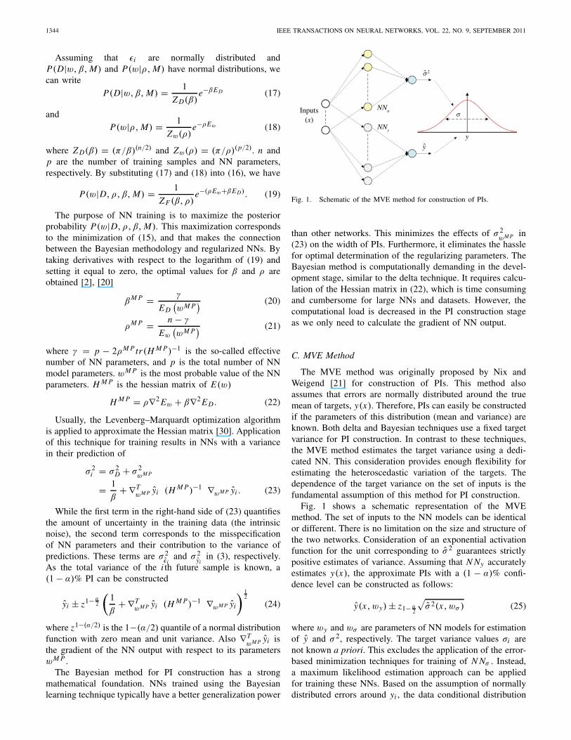
Fig. 1. Schematic of the MVE method for construction of PIs.

than other networks. This minimizes the effects of σ 2wM P in

(23) on the width of PIs. Furthermore, it eliminates the hasslefor optimal determination of the regularizing parameters. TheBayesian method is computationally demanding in the devel-opment stage, similar to the delta technique. It requires calcu-lation of the Hessian matrix in (22), which is time consumingand cumbersome for large NNs and datasets. However, thecomputational load is decreased in the PI construction stageas we only need to calculate the gradient of NN output.

C. MVE Method

The MVE method was originally proposed by Nix andWeigend [21] for construction of PIs. This method alsoassumes that errors are normally distributed around the truemean of targets, y(x). Therefore, PIs can easily be constructedif the parameters of this distribution (mean and variance) areknown. Both delta and Bayesian techniques use a fixed targetvariance for PI construction. In contrast to these techniques,the MVE method estimates the target variance using a dedi-cated NN. This consideration provides enough flexibility forestimating the heteroscedastic variation of the targets. Thedependence of the target variance on the set of inputs is thefundamental assumption of this method for PI construction.

Fig. 1 shows a schematic representation of the MVEmethod. The set of inputs to the NN models can be identicalor different. There is no limitation on the size and structure ofthe two networks. Consideration of an exponential activationfunction for the unit corresponding to σ 2 guarantees strictlypositive estimates of variance. Assuming that N Ny accuratelyestimates y(x), the approximate PIs with a (1 − α)% confi-dence level can be constructed as follows:

y(x, wy) ± z1− α2

√σ 2(x, wσ ) (25)

where wy and wσ are parameters of NN models for estimationof y and σ 2, respectively. The target variance values σi arenot known a priori. This excludes the application of the error-based minimization techniques for training of N Nσ . Instead,a maximum likelihood estimation approach can be appliedfor training these NNs. Based on the assumption of normallydistributed errors around yi , the data conditional distribution

KHOSRAVI et al.: REVIEW OF NN-BASED PREDICTION INTERVALS AND NEW ADVANCES 1345

will be

P(ti | xi , N Ny , N Nσ ) = 1√2πσ 2

i

e− (ti −yi )

2

2σ2i . (26)

Taking the natural log of this distribution and ignoring theconstant terms result in the following cost function, which willbe minimized for all samples:

CMV E = 1

2

n∑i=1

[ln(σ 2

i ) +(ti − yi

)2

σ 2i

]. (27)

Using this cost function, an indirect three-phase trainingtechnique was proposed in [21] for simultaneously adjustingwy and wσ . The proposed algorithm needs two datasets,namely, D1 and D2, for training N Ny and N Nσ . In Phase I ofthe training algorithm, N Ny is trained to estimate yi . Trainingis performed through minimization of an error-based cost func-tion for the first dataset D1. To avoid the overfitting problem,D2 can be used as the validation set and for terminating thetraining algorithm. Nothing is done with N Nσ in this phase. InPhase II, wy are fixed, and D2 is used for adjusting parametersof N Nσ . Adjusting of wσ is achieved through minimizingthe cost function defined in (27). N Ny and N Nσ are used toapproximate yi and σ 2 for each sample, respectively. The costfunction is then evaluated for the current set of N Nσ weightswσ . These weights then are updated using the traditionalgradient-descent-based methods. D1 can also be applied as thevalidation set to limit the overfitting effects. In Phase III, twonew training sets are resampled and applied for simultaneousadjustment of both network parameters. The retraining of N Ny

and N Nσ is again carried out through minimization of (27).As before, one of the sets is used as the validation set.

The main advantage of this method is its simplicity, andthat there is no need to calculate complex derivatives and theinversion of the Hessian matrix. Nonstationary variances canbe approximated by employing more complex structures forN Nσ or through proper selection of the set of inputs.

The main drawback of the MVE method is that it assumesN Ny precisely estimates the true mean of the targets, i.e.,yi . This assumption can be violated in practice because of avariety of reasons, including the existence of a bias in fittingthe data due to a possible underspecification of the NN modelor due to omission of important attributes affecting the targetbehavior. In these cases, the NN generalization power is weak,resulting in accumulation of uncertainty in the estimation of yi .Therefore, the constructed PIs using (25) will underestimate(or overestimate) the actual (1 − α)% PIs, leading to a lowcoverage probability.

Assuming yi � yi implies that the MVE method onlyconsiders one portion of the total uncertainty for constructionof PIs. The considered variance is only due to errors, not dueto misspecification of model parameters (either wy or wσ ).This can result in misleadingly narrow PIs with a low cover-age probability. This critical drawback has been theoreticallyidentified and practically demonstrated in the literature [31].

OriginalTrainingDataset

D1

NN1

NN2

NNB

D2

DB

y1

y�

�

y2

yB

σy2

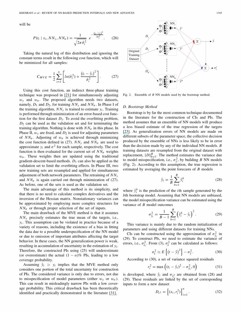
Fig. 2. Ensemble of B NN models used by the bootstrap method.

D. Bootstrap Method

Bootstrap is by far the most common technique documentedin the literature for the construction of CIs and PIs. Themethod assumes that an ensemble of NN models will producea less biased estimate of the true regression of the targets[23]. As generalization errors of NN models are made ondifferent subsets of the parameter space, the collective decisionproduced by the ensemble of NNs is less likely to be in errorthan the decision made by any of the individual NN models. Btraining datasets are resampled from the original dataset withreplacement, {D}B

b=1. The method estimates the variance dueto model misspecification, i.e., σ 2

y , by building B NN models(Fig. 2). According to this assumption, the true regression isestimated by averaging the point forecasts of B models

yi = 1

B

B∑b=1

ybi (28)

where ybi is the prediction of the i th sample generated by the

bth bootstrap model. Assuming that NN models are unbiased,the model misspecification variance can be estimated using thevariance of B model outcomes

σ 2yi

= 1

B − 1

B∑b=1

(yb

i − yi

)2. (29)

This variance is mainly due to the random initialization ofparameters and using different datasets for training NNs.

CIs can be constructed using the approximation of σ 2yi

in(29). To construct PIs, we need to estimate the variance oferrors, i.e., σ 2

εi. From (3), σ 2

εcan be calculated as follows:

σ 2ε � E

{(t − y

)2}

− σ 2y . (30)

According to (30), a set of variance squared residuals

r2i = max

((ti − yi )

2 − σ 2yi, 0

)(31)

is developed, where yi and σy2i

are obtained from (28) and(29). These residuals are linked by the set of correspondinginputs to form a new dataset

Dr2 ={(xi , r2

i )}n

i=1. (32)

1346 IEEE TRANSACTIONS ON NEURAL NETWORKS, VOL. 22, NO. 9, SEPTEMBER 2011

A new NN model can be indirectly trained to estimate theunknown values of σ 2

εi, so as to maximize the probability

of observing the samples in Dr2 . The procedure for indirecttraining of this new NN is very similar to the steps of the MVEmethod described in Section II-C. The training cost functionis defined as

CBS = 1

2

n∑i=1

[ln(σ 2

εi) + r2

i

σ 2εi

]. (33)

As noted before, the NN output node activation functionis selected to be exponential, enforcing a positive value forσ 2

εi. The minimization of CBS can be done using a variety of

methods, including traditional gradient descent methods.The described bootstrap method is traditionally called the

bootstrap pairs. There exists another bootstrap method, calledbootstrap residuals, which resamples the prediction residuals.Further information on this method can be found in [29].

For construction of PIs using the bootstrap method, B + 1NN models are required in total. B NN models (assumedto be unbiased) are used for estimation of σy2

iand one

model is used for estimation of σ 2εi

. Therefore, this methodis computationally more demanding than other methods in itsdevelopment stage (B + 1 times more). However, once themodels are trained offline, the online computational load forPI construction is only limited to B + 1 NN point forecasts.This is in contrast with the claim in the literature that bootstrapPIs are computationally more intensive than other methods[27]. This claim will be precisely verified in the later sections.Simplicity is another advantage of using the Bootstrap methodfor PI construction. There is no need to calculate complexmatrices and derivatives, as required by the delta and Bayesiantechniques.

The main disadvantage of the bootstrap technique is itsdependence on B NN models. Frequently some of thesemodels are biased, leading to an inaccurate estimation of σ 2

yiin (29). Therefore, the total variance will be underestimatedresulting in narrow PIs with a low coverage probability.

III. PI ASSESSMENT MEASURES

Discussion in the literature on the quality of constructed PIsis often vague and incomplete [8], [9], [11], [14], [18], [21],[26], [27]. Frequently, PIs are assessed from their coverageprobability perspective without any discussion about how widethey are. As discussed in [10] and [32], such an assessmentis subjective and can lead to misleading results. Here webriefly discuss two indices for quantitative and comprehensiveassessment of PIs.

The most important characteristic of PIs is their coverageprobability. PI coverage probability (PICP) is measured bycounting the number of target values covered by the con-structed PIs

P IC P = 1

ntest

ntest∑i=1

ci (34)

where

ci =⎧⎨⎩

1, ti ∈ [Li , Ui ]

0, ti /∈ [Li , Ui ](35)

where ntest is the number of samples in the test set, and Li

and Ui are lower and upper bounds of the i th PI, respectively.Ideally, PICP should be very close or larger than the nominalconfidence level associated to the PIs.

PICP has a direct relationship with the width of PIs. Asatisfactorily large PICP can be easily achieved by wideningPIs from either side. However, such PIs are too conservativeand less useful in practice, as they do not show the variationof the targets. Therefore, a measure is required to check howwide the PIs are. Mean PI width (MPIW) quantifies this aspectof PIs [10]

MPIW = 1

ntest

ntest∑i=1

(Ui − Li ) . (36)

MPIW shows the average width of PIs. Normalizing MPIWby the range R of the underlying target allows us to comparePIs constructed for different datasets respectively (the newmeasure is called NMPIW)

NMPIW = MPIW

R. (37)

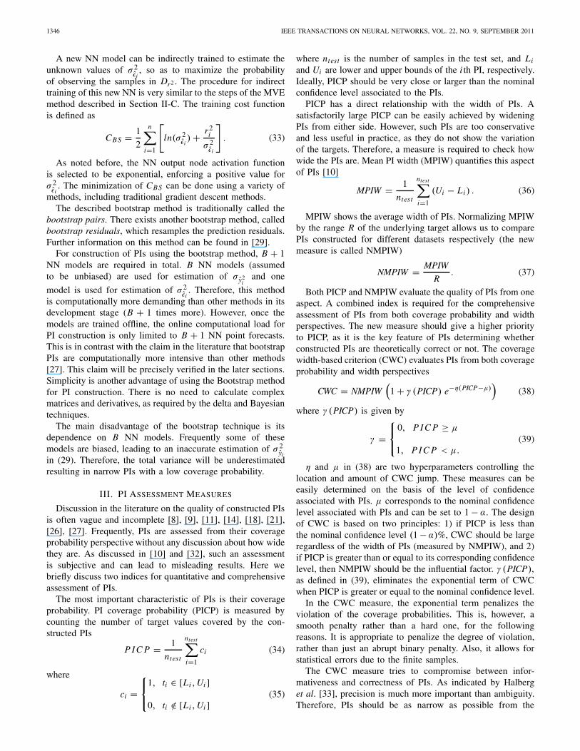
Both PICP and NMPIW evaluate the quality of PIs from oneaspect. A combined index is required for the comprehensiveassessment of PIs from both coverage probability and widthperspectives. The new measure should give a higher priorityto PICP, as it is the key feature of PIs determining whetherconstructed PIs are theoretically correct or not. The coveragewidth-based criterion (CWC) evaluates PIs from both coverageprobability and width perspectives

CWC = NMPIW(

1 + γ (PICP) e−η(PICP−μ))

(38)

where γ (PICP) is given by

γ =⎧⎨⎩

0, P IC P ≥ μ

1, P IC P < μ.(39)

η and μ in (38) are two hyperparameters controlling thelocation and amount of CWC jump. These measures can beeasily determined on the basis of the level of confidenceassociated with PIs. μ corresponds to the nominal confidencelevel associated with PIs and can be set to 1 − α. The designof CWC is based on two principles: 1) if PICP is less thanthe nominal confidence level (1 − α)%, CWC should be largeregardless of the width of PIs (measured by NMPIW), and 2)if PICP is greater than or equal to its corresponding confidencelevel, then NMPIW should be the influential factor. γ (PICP),as defined in (39), eliminates the exponential term of CWCwhen PICP is greater or equal to the nominal confidence level.

In the CWC measure, the exponential term penalizes theviolation of the coverage probabilities. This is, however, asmooth penalty rather than a hard one, for the followingreasons. It is appropriate to penalize the degree of violation,rather than just an abrupt binary penalty. Also, it allows forstatistical errors due to the finite samples.

The CWC measure tries to compromise between infor-mativeness and correctness of PIs. As indicated by Halberget al. [33], precision is much more important than ambiguity.Therefore, PIs should be as narrow as possible from the

KHOSRAVI et al.: REVIEW OF NN-BASED PREDICTION INTERVALS AND NEW ADVANCES 1347

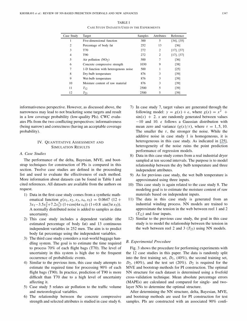
TABLE I

CASE STUDY DATASETS USED IN THE EXPERIMENTS

Case Study Target Samples Attributes Reference

1 Five-dimensional function 300 5 [34], [35]

2 Percentage of body fat 252 13 [36]

3 T70 272 2 [17], [37]

4 T90 272 2 [17], [37]

5 Air pollution (NO2) 500 7 [36]

6 Concrete compressive strength 1030 9 [38]

7 1-D function with heterogenous noise 500 1 [25]

8 Dry-bulb temperature 876 3 [39]

9 Wet-bulb temperature 876 3 [39]

10 Moisture content of raw material 876 3 [39]

11 T12 2500 5 [39]

12 T23 2500 5 [39]

informativeness perspective. However, as discussed above, thenarrowness may lead to not bracketing some targets and resultin a low coverage probability (low-quality PIs). CWC evalu-ates PIs from the two conflicting perspectives: informativeness(being narrow) and correctness (having an acceptable coverageprobability).

IV. QUANTITATIVE ASSESSMENT AND

SIMULATION RESULTS

A. Case Studies

The performance of the delta, Bayesian, MVE, and boot-strap techniques for construction of PIs is compared in thissection. Twelve case studies are defined in the proceedinglist and used to evaluate the effectiveness of each method.More information about datasets can be found in Table I andcited references. All datasets are available from the authors onrequest.

1) Data in the first case study comes from a synthetic math-ematical function g(x1, x2, x3, x4, x5) = 0.0647 (12 +3x1−3.5x2

2+7.2x33) (1+cos(4πx4)) (1+0.8 sin(3πx5)).

A normally distributed noise is added to samples as datauncertainty.

2) This case study includes a dependent variable (theestimated percentage of body fat) and 13 continuousindependent variables in 252 men. The aim is to predictbody fat percentage using the independent variables.

3) The third case study considers a real-world baggage han-dling system. The goal is to estimate the time requiredto process 70% of each flight bags (T70). The level ofuncertainty in this system is high due to the frequentoccurrence of probabilistic events.

4) Similar to the previous item, this case study attempts toestimate the required time for processing 90% of eachflight bags (T90). In practice, prediction of T90 is moredifficult than T70 due to a high level of uncertaintyaffecting it.

5) Case study 5 relates air pollution to the traffic volumeand meteorological variables.

6) The relationship between the concrete compressivestrength and selected attributes is studied in case study 6.

7) In case study 7, target values are generated through thefollowing model: y = g(x) + ε, where g(x) = x2 +sin(x) + 2. x are randomly generated between values−10 and 10. ε follows a Gaussian distribution withmean zero and variance (g(x)/τ ), where τ = 1, 5, 10.The smaller the τ , the stronger the noise. While theadditive noise in case study 1 is homogeneous, it isheterogeneous in this case study. As indicated in [25],heterogeneity of the noise ruins the point predictionperformance of regression models.

8) Data in this case study comes from a real industrial dryersampled at ten second intervals. The purpose is to modelrelationship between the dry bulb temperature and threeindependent attributes.

9) As for previous case study, the wet bulb temperature isapproximated using three inputs.

10) This case study is again related to the case study 8. Themodeling goal is to estimate the moisture content of rawmaterials based on independent inputs.

11) The data in this case study is generated from anindustrial winding process. NN models are trained toapproximate the tension in the web between reel 1 and 2(T12) and four inputs.

12) Similar to the previous case study, the goal in this casestudy is to model the relationship between the tension inthe web between reel 2 and 3 (T23) using NN models.

B. Experimental Procedure

Fig. 3 shows the procedure for performing experiments withthe 12 case studies in this paper. The data is randomly splitinto the first training set, D1, (40%), the second training set,D2, (40%), and the test set (20%). D2 is required for theMVE and bootstrap methods for PI construction. The optimalNN structure for each dataset is determined using a fivefoldcross-validation technique. Mean absolute percentage errors(MAPEs) are calculated and compared for single- and two-layer NNs to determine the optimal structure.

After determining the NN structure, delta, Bayesian, MVE,and bootstrap methods are used for PI construction for testsamples. PIs are constructed with an associated 90% confi-

1348 IEEE TRANSACTIONS ON NEURAL NETWORKS, VOL. 22, NO. 9, SEPTEMBER 2011

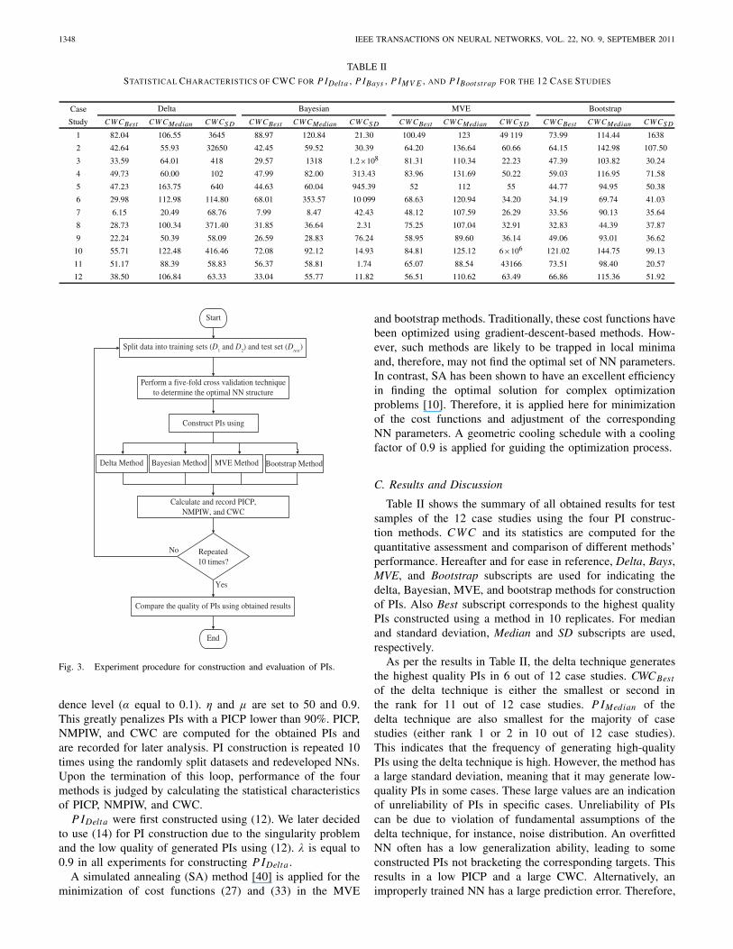
TABLE II

STATISTICAL CHARACTERISTICS OF CWC FOR P IDelta , P IBays , P IMV E , AND P IBootstrap FOR THE 12 CASE STUDIES

Case Delta Bayesian MVE Bootstrap

Study CWCBest CWCMedian CWCS D CWCBest CWCMedian CWCS D CWCBest CWCMedian CWCS D CWCBest CWCMedian CWCS D

1 82.04 106.55 3645 88.97 120.84 21.30 100.49 123 49 119 73.99 114.44 1638

2 42.64 55.93 32650 42.45 59.52 30.39 64.20 136.64 60.66 64.15 142.98 107.50

3 33.59 64.01 418 29.57 1318 1.2×108 81.31 110.34 22.23 47.39 103.82 30.24

4 49.73 60.00 102 47.99 82.00 313.43 83.96 131.69 50.22 59.03 116.95 71.58

5 47.23 163.75 640 44.63 60.04 945.39 52 112 55 44.77 94.95 50.38

6 29.98 112.98 114.80 68.01 353.57 10 099 68.63 120.94 34.20 34.19 69.74 41.03

7 6.15 20.49 68.76 7.99 8.47 42.43 48.12 107.59 26.29 33.56 90.13 35.64

8 28.73 100.34 371.40 31.85 36.64 2.31 75.25 107.04 32.91 32.83 44.39 37.87

9 22.24 50.39 58.09 26.59 28.83 76.24 58.95 89.60 36.14 49.06 93.01 36.62

10 55.71 122.48 416.46 72.08 92.12 14.93 84.81 125.12 6×106 121.02 144.75 99.13

11 51.17 88.39 58.83 56.37 58.81 1.74 65.07 88.54 43166 73.51 98.40 20.57

12 38.50 106.84 63.33 33.04 55.77 11.82 56.51 110.62 63.49 66.86 115.36 51.92

Yes

Start

Split data into training sets (D1 and D

2) and test set (D

test)

Construct PIs using

Delta Method

Calculate and record PICP,NMPIW, and CWC

Repeated10 times?

No

Compare the quality of PIs using obtained results

End

MVE MethodBayesian Method Bootstrap Method

Perform a five-fold cross validation techniqueto determine the optimal NN structure

Fig. 3. Experiment procedure for construction and evaluation of PIs.

dence level (α equal to 0.1). η and μ are set to 50 and 0.9.This greatly penalizes PIs with a PICP lower than 90%. PICP,NMPIW, and CWC are computed for the obtained PIs andare recorded for later analysis. PI construction is repeated 10times using the randomly split datasets and redeveloped NNs.Upon the termination of this loop, performance of the fourmethods is judged by calculating the statistical characteristicsof PICP, NMPIW, and CWC.

P IDelta were first constructed using (12). We later decidedto use (14) for PI construction due to the singularity problemand the low quality of generated PIs using (12). λ is equal to0.9 in all experiments for constructing P IDelta .

A simulated annealing (SA) method [40] is applied for theminimization of cost functions (27) and (33) in the MVE

and bootstrap methods. Traditionally, these cost functions havebeen optimized using gradient-descent-based methods. How-ever, such methods are likely to be trapped in local minimaand, therefore, may not find the optimal set of NN parameters.In contrast, SA has been shown to have an excellent efficiencyin finding the optimal solution for complex optimizationproblems [10]. Therefore, it is applied here for minimizationof the cost functions and adjustment of the correspondingNN parameters. A geometric cooling schedule with a coolingfactor of 0.9 is applied for guiding the optimization process.

C. Results and Discussion

Table II shows the summary of all obtained results for testsamples of the 12 case studies using the four PI construc-tion methods. CWC and its statistics are computed for thequantitative assessment and comparison of different methods’performance. Hereafter and for ease in reference, Delta, Bays,MVE, and Bootstrap subscripts are used for indicating thedelta, Bayesian, MVE, and bootstrap methods for constructionof PIs. Also Best subscript corresponds to the highest qualityPIs constructed using a method in 10 replicates. For medianand standard deviation, Median and SD subscripts are used,respectively.

As per the results in Table II, the delta technique generatesthe highest quality PIs in 6 out of 12 case studies. CWCBest

of the delta technique is either the smallest or second inthe rank for 11 out of 12 case studies. P IMedian of thedelta technique are also smallest for the majority of casestudies (either rank 1 or 2 in 10 out of 12 case studies).This indicates that the frequency of generating high-qualityPIs using the delta technique is high. However, the method hasa large standard deviation, meaning that it may generate low-quality PIs in some cases. These large values are an indicationof unreliability of PIs in specific cases. Unreliability of PIscan be due to violation of fundamental assumptions of thedelta technique, for instance, noise distribution. An overfittedNN often has a low generalization ability, leading to someconstructed PIs not bracketing the corresponding targets. Thisresults in a low PICP and a large CWC. Alternatively, animproperly trained NN has a large prediction error. Therefore,

KHOSRAVI et al.: REVIEW OF NN-BASED PREDICTION INTERVALS AND NEW ADVANCES 1349

DeltaBayesianMVE

PIC

P105

100

95

90

85

NM

PIW

14012010080604020

0

Case Studies1 2 3 4 5 6 7 8 9 10 11 12

Case Studies1 2 3 4 5 6 7 8 9 10 11 12

Bootstrap

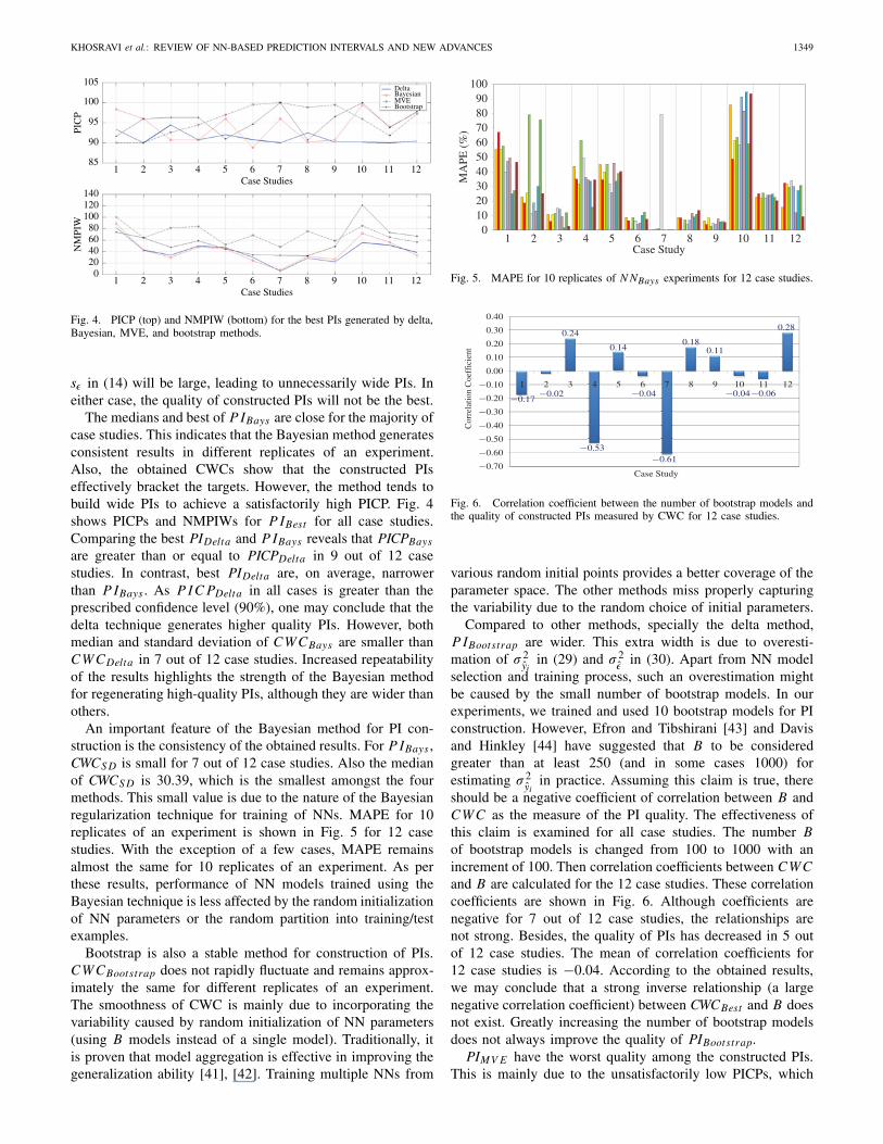
Fig. 4. PICP (top) and NMPIW (bottom) for the best PIs generated by delta,Bayesian, MVE, and bootstrap methods.

sε in (14) will be large, leading to unnecessarily wide PIs. Ineither case, the quality of constructed PIs will not be the best.

The medians and best of P IBays are close for the majority ofcase studies. This indicates that the Bayesian method generatesconsistent results in different replicates of an experiment.Also, the obtained CWCs show that the constructed PIseffectively bracket the targets. However, the method tends tobuild wide PIs to achieve a satisfactorily high PICP. Fig. 4shows PICPs and NMPIWs for P IBest for all case studies.Comparing the best PIDelta and P IBays reveals that PICPBays

are greater than or equal to PICPDelta in 9 out of 12 casestudies. In contrast, best PIDelta are, on average, narrowerthan P IBays . As P IC PDelta in all cases is greater than theprescribed confidence level (90%), one may conclude that thedelta technique generates higher quality PIs. However, bothmedian and standard deviation of CWCBays are smaller thanCWCDelta in 7 out of 12 case studies. Increased repeatabilityof the results highlights the strength of the Bayesian methodfor regenerating high-quality PIs, although they are wider thanothers.

An important feature of the Bayesian method for PI con-struction is the consistency of the obtained results. For P IBays ,CWCS D is small for 7 out of 12 case studies. Also the medianof CWCS D is 30.39, which is the smallest amongst the fourmethods. This small value is due to the nature of the Bayesianregularization technique for training of NNs. MAPE for 10replicates of an experiment is shown in Fig. 5 for 12 casestudies. With the exception of a few cases, MAPE remainsalmost the same for 10 replicates of an experiment. As perthese results, performance of NN models trained using theBayesian technique is less affected by the random initializationof NN parameters or the random partition into training/testexamples.

Bootstrap is also a stable method for construction of PIs.CWCBootstrap does not rapidly fluctuate and remains approx-imately the same for different replicates of an experiment.The smoothness of CWC is mainly due to incorporating thevariability caused by random initialization of NN parameters(using B models instead of a single model). Traditionally, itis proven that model aggregation is effective in improving thegeneralization ability [41], [42]. Training multiple NNs from

0102030405060708090

100

1 2 3 4 5 6 7 8 9 10 11 12

MA

PE (

%)

Case Study

Fig. 5. MAPE for 10 replicates of N NBays experiments for 12 case studies.

−0.17−0.02

0.24

−0.53

0.14

−0.04

−0.61

0.180.11

−0.04−0.06

0.28

−0.70

−0.60

−0.50

−0.40

−0.30

−0.20

−0.10

0.00

0.10

0.20

0.30

0.40

1 2 3 4 5 6 7 8 9 10 11 12

Cor

rela

tion

Coe

ffic

ient

Case Study

Fig. 6. Correlation coefficient between the number of bootstrap models andthe quality of constructed PIs measured by CWC for 12 case studies.

various random initial points provides a better coverage of theparameter space. The other methods miss properly capturingthe variability due to the random choice of initial parameters.

Compared to other methods, specially the delta method,P IBootstrap are wider. This extra width is due to overesti-mation of σ 2

yiin (29) and σ 2

εin (30). Apart from NN model

selection and training process, such an overestimation mightbe caused by the small number of bootstrap models. In ourexperiments, we trained and used 10 bootstrap models for PIconstruction. However, Efron and Tibshirani [43] and Davisand Hinkley [44] have suggested that B to be consideredgreater than at least 250 (and in some cases 1000) forestimating σ 2

yiin practice. Assuming this claim is true, there

should be a negative coefficient of correlation between B andCWC as the measure of the PI quality. The effectiveness ofthis claim is examined for all case studies. The number Bof bootstrap models is changed from 100 to 1000 with anincrement of 100. Then correlation coefficients between CWCand B are calculated for the 12 case studies. These correlationcoefficients are shown in Fig. 6. Although coefficients arenegative for 7 out of 12 case studies, the relationships arenot strong. Besides, the quality of PIs has decreased in 5 outof 12 case studies. The mean of correlation coefficients for12 case studies is −0.04. According to the obtained results,we may conclude that a strong inverse relationship (a largenegative correlation coefficient) between CWCBest and B doesnot exist. Greatly increasing the number of bootstrap modelsdoes not always improve the quality of PIBootstrap.

PIMV E have the worst quality among the constructed PIs.This is mainly due to the unsatisfactorily low PICPs, which

1350 IEEE TRANSACTIONS ON NEURAL NETWORKS, VOL. 22, NO. 9, SEPTEMBER 2011

1.5

150 160 170 180

Delta Bayesian

Samples Samples

Samples Samples

MVE Bootstrap

190 200

150 160 170 180 190 200

150 160 170 180 190 200

150 160 170 180 190 200

1

0.5

0

Con

cret

e St

reng

th

−0.5

−1

−1.5

1.5

1

0.5

0

Con

cret

e St

reng

th

−0.5

−1

−1.5

2

1.5

1

0.5

0

Con

cret

e St

reng

th

−0.5

−1

−2

−1.5

1.5

1

0.5

0

Con

cret

e St

reng

th

−0.5

−1

−1.5

Fig. 7. P IMedian constructed for case study 6 using the delta method (top left), the Bayesian method (top right), the MVE method (bottom left), and thebootstrap method (bottom right).

stems from the improper estimation of the target variance usingthe NN models. It is highly likely that the target variancehas little systematic relationship with the inputs. Even ifthere exists a relationship, some important variables may bemissing. Another source of problem can be the invalidity ofthe fundamental assumption of the MVE method ( yi � yi ).This assumption can be violated for many reasons, speciallyfor practical cases. Misspecification of NN model parameters,non-optimal selection of the NN architecture, and impropertraining of the NN model are among the potential causes.

It is also important to observe how the widths of PIs changefor different observations of a target. The variability of thewidths of PIs is an indication of how well they respondto the level of uncertainty in the datasets. Practically, weexpect wider PIs for cases in which there is more uncer-tainty in datasets (e.g., having multivalued targets for approx-imately equal conditions or a high level of noise affectingthe targets). Fig. 7 shows P IMedian for the delta, Bayesian,MVE, and bootstrap methods calculated for case study 6.1

Comparing P IDelta with others points out that P IDelta areapproximately constant in width and only their centers go upand down (which are in fact the point forecasts generatedby the NN model). From the mathematical point of view,it means gT

0 (FT F + λI )−1(FT F)(FT F + λI )−1g0 � 1,and therefore the width of P IDelta is mainly affected bysε . A similar story happens for the Bayesian method, thewidth of PIBays is dominated by (1/β) in (24) ((1/β) ∇T

wM P yi (H M P)−1 ∇wM P yi ). The MVE and bootstrap

1For better visualization, only PIs for samples 150 to 200 are shown.

TABLE III

COV FOR P IMedian CONSTRUCTED USING THE DELTA, BAYESIAN,

MVE, AND BOOTSTRAP METHODS

Case StudyCOV

Delta Bayesian MVE Bootstrap

1 2.40 2.75 7.77 8.45

2 7.38 8.27 8.95 10.94

3 8.41 15.02 12.88 16.77

4 5.06 7.29 12.65 20.25

5 6.82 6.49 12.46 13.80

6 6.04 7.35 8.22 14.46

7 42.75 36.39 14.17 18.59

8 9.61 4.20 11.32 19.83

9 8.10 3.36 10.63 11.57

10 3.12 1.75 12.11 8.44

11 1.75 4.50 11.08 12.17

12 9.17 8.70 13.03 12.72

methods show a better performance and their PIs have morevariable widths. These variable widths imply that the estima-tion of variances using NNs enables the methods to appropri-ately respond to the level of uncertainty in the data.

The coefficient of variations (COVs) (ratio of the standarddeviation to the mean) for the width of PIMedian constructedusing the delta, Bayesian, MVE, and bootstrap are shownin Table III. According to these statistics, PIBootstrap havethe largest variability in the width. The MVE method alsoshows an acceptable performance in terms of variable widthsof PIs. P IDelta and P IBays have the lowest COVs, which are

KHOSRAVI et al.: REVIEW OF NN-BASED PREDICTION INTERVALS AND NEW ADVANCES 1351

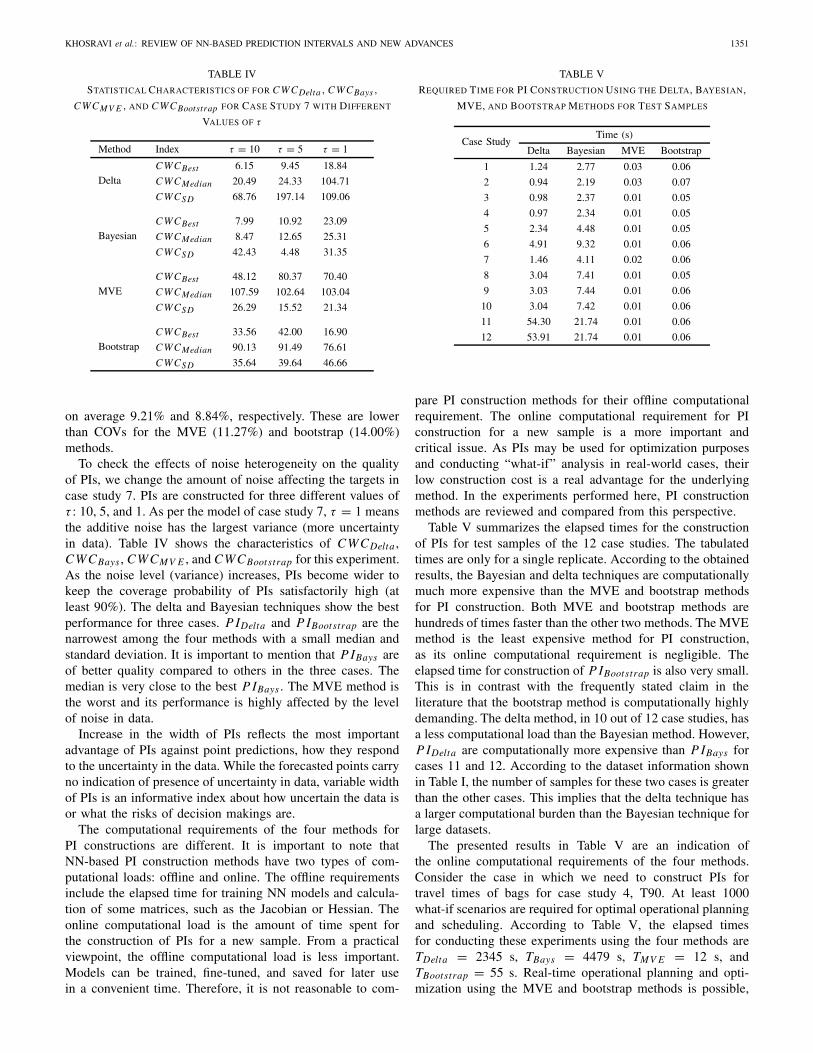
TABLE IV

STATISTICAL CHARACTERISTICS OF FOR CWCDelta , CWCBays ,

CWCMV E , AND CWCBootstrap FOR CASE STUDY 7 WITH DIFFERENT

VALUES OF τ

Method Index τ = 10 τ = 5 τ = 1

DeltaCWCBest 6.15 9.45 18.84

CWCMedian 20.49 24.33 104.71

CWCSD 68.76 197.14 109.06

BayesianCWCBest 7.99 10.92 23.09

CWCMedian 8.47 12.65 25.31

CWCSD 42.43 4.48 31.35

MVECWCBest 48.12 80.37 70.40

CWCMedian 107.59 102.64 103.04

CWCSD 26.29 15.52 21.34

BootstrapCWCBest 33.56 42.00 16.90

CWCMedian 90.13 91.49 76.61

CWCSD 35.64 39.64 46.66

on average 9.21% and 8.84%, respectively. These are lowerthan COVs for the MVE (11.27%) and bootstrap (14.00%)methods.

To check the effects of noise heterogeneity on the qualityof PIs, we change the amount of noise affecting the targets incase study 7. PIs are constructed for three different values ofτ : 10, 5, and 1. As per the model of case study 7, τ = 1 meansthe additive noise has the largest variance (more uncertaintyin data). Table IV shows the characteristics of CWCDelta ,CWCBays , CWCMV E , and CWCBootstrap for this experiment.As the noise level (variance) increases, PIs become wider tokeep the coverage probability of PIs satisfactorily high (atleast 90%). The delta and Bayesian techniques show the bestperformance for three cases. P IDelta and P IBootstrap are thenarrowest among the four methods with a small median andstandard deviation. It is important to mention that P IBays areof better quality compared to others in the three cases. Themedian is very close to the best P IBays . The MVE method isthe worst and its performance is highly affected by the levelof noise in data.

Increase in the width of PIs reflects the most importantadvantage of PIs against point predictions, how they respondto the uncertainty in the data. While the forecasted points carryno indication of presence of uncertainty in data, variable widthof PIs is an informative index about how uncertain the data isor what the risks of decision makings are.

The computational requirements of the four methods forPI constructions are different. It is important to note thatNN-based PI construction methods have two types of com-putational loads: offline and online. The offline requirementsinclude the elapsed time for training NN models and calcula-tion of some matrices, such as the Jacobian or Hessian. Theonline computational load is the amount of time spent forthe construction of PIs for a new sample. From a practicalviewpoint, the offline computational load is less important.Models can be trained, fine-tuned, and saved for later usein a convenient time. Therefore, it is not reasonable to com-

TABLE V

REQUIRED TIME FOR PI CONSTRUCTION USING THE DELTA, BAYESIAN,

MVE, AND BOOTSTRAP METHODS FOR TEST SAMPLES

Case StudyTime (s)

Delta Bayesian MVE Bootstrap

1 1.24 2.77 0.03 0.06

2 0.94 2.19 0.03 0.07

3 0.98 2.37 0.01 0.05

4 0.97 2.34 0.01 0.05

5 2.34 4.48 0.01 0.05

6 4.91 9.32 0.01 0.06

7 1.46 4.11 0.02 0.06

8 3.04 7.41 0.01 0.05

9 3.03 7.44 0.01 0.06

10 3.04 7.42 0.01 0.06

11 54.30 21.74 0.01 0.06

12 53.91 21.74 0.01 0.06

pare PI construction methods for their offline computationalrequirement. The online computational requirement for PIconstruction for a new sample is a more important andcritical issue. As PIs may be used for optimization purposesand conducting “what-if” analysis in real-world cases, theirlow construction cost is a real advantage for the underlyingmethod. In the experiments performed here, PI constructionmethods are reviewed and compared from this perspective.

Table V summarizes the elapsed times for the constructionof PIs for test samples of the 12 case studies. The tabulatedtimes are only for a single replicate. According to the obtainedresults, the Bayesian and delta techniques are computationallymuch more expensive than the MVE and bootstrap methodsfor PI construction. Both MVE and bootstrap methods arehundreds of times faster than the other two methods. The MVEmethod is the least expensive method for PI construction,as its online computational requirement is negligible. Theelapsed time for construction of P IBootstrap is also very small.This is in contrast with the frequently stated claim in theliterature that the bootstrap method is computationally highlydemanding. The delta method, in 10 out of 12 case studies, hasa less computational load than the Bayesian method. However,P IDelta are computationally more expensive than P IBays forcases 11 and 12. According to the dataset information shownin Table I, the number of samples for these two cases is greaterthan the other cases. This implies that the delta technique hasa larger computational burden than the Bayesian technique forlarge datasets.

The presented results in Table V are an indication ofthe online computational requirements of the four methods.Consider the case in which we need to construct PIs fortravel times of bags for case study 4, T90. At least 1000what-if scenarios are required for optimal operational planningand scheduling. According to Table V, the elapsed timesfor conducting these experiments using the four methods areTDelta = 2345 s, TBays = 4479 s, TMV E = 12 s, andTBootstrap = 55 s. Real-time operational planning and opti-mization using the MVE and bootstrap methods is possible,

1352 IEEE TRANSACTIONS ON NEURAL NETWORKS, VOL. 22, NO. 9, SEPTEMBER 2011

as both TMV E and TBootstrap are less than 1 min. The deltaand Bayesian methods do not finish their online computationin a practical time, and are therefore not suitable for real-timeoperational planning in a baggage handling system.

Decision regarding the suitability of a PI construc-tion method for optimization and decision-making purposesdepends on the size of dataset and constraints of the underlyingsystem. For instance, while the delta and Bayesian methods arenot the best option for case studies 3 and 4, they can be easilyapplied to case studies 8–10. The PI construction methods haveenough time to compute the required calculations, as the rateof completion of the tasks and operations for this case study isslow. Therefore, the operational planners and schedulers canenjoy the excellent quality of P IDelta and P IBays withoutconsidering the computational load.

D. Summary

To quantify the performance of the PI construction methods,we rank each method from 1 to 4 depending on the constructedPIs for test samples. The lower the rank, the better the method.The ranking scores are given in four categories as per thefollowing.

1) Quality: CWCMedian is used as an index to quantify theperformance of each method for producing high qualityPIs. For each case study, CWCMedian in Table II aresorted increasingly and scored between 1 (the lowest)and 4 (the greatest) for the four PI construction methods.The scores are then averaged to generate a total scoreof the method’s performance.

2) Repeatability: This is measured by calculating the 70thpercentile of CWC (i.e., seventh best replicate). As aconservative measure, this provides information abouthow each method will do in worst cases, which methodsare prone to fail, and which methods do well even intheir bad runs. Similar to the quality metric, the 70thpercentiles are sorted, scored between 1 and 4, and thenaveraged for twelve case studies.

3) Computational load: The same scoring method is appliedto the elapsed times as shown in Table V.

4) Variability: This metric relates to the response of PIs tothe level of uncertainty associated with data. To measurethis, we first obtain the width of P IBest for the delta,Bayesian, MVE, and bootstrap techniques. Then, theCOV is calculated for this set as an indication of itsvariation. The method with the greatest COV is scored1, the method corresponding to the second greatest COVis scored 2, and so on.

It is important to observe that these metrics have unequalimportance in practice. While the PI quality is the mostimportant metric for some decision makers, the computationalload can be the key factor in optimization problems.

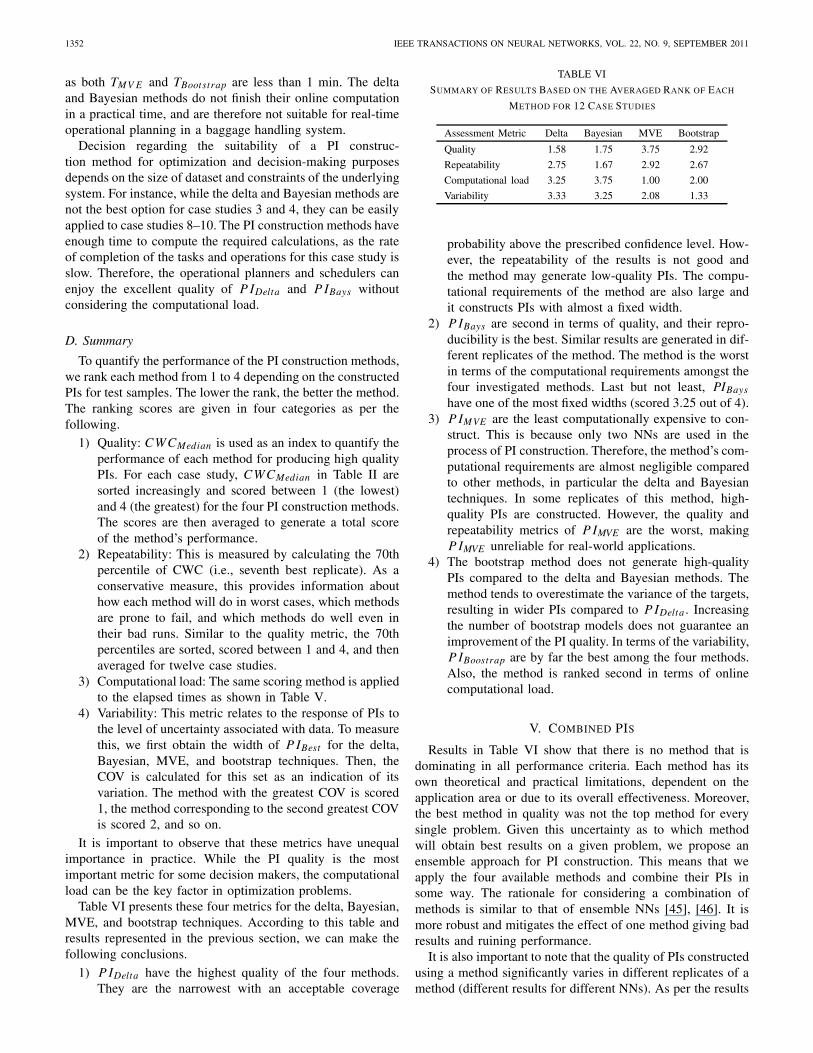
Table VI presents these four metrics for the delta, Bayesian,MVE, and bootstrap techniques. According to this table andresults represented in the previous section, we can make thefollowing conclusions.

1) P IDelta have the highest quality of the four methods.They are the narrowest with an acceptable coverage

TABLE VI

SUMMARY OF RESULTS BASED ON THE AVERAGED RANK OF EACH

METHOD FOR 12 CASE STUDIES

Assessment Metric Delta Bayesian MVE Bootstrap

Quality 1.58 1.75 3.75 2.92

Repeatability 2.75 1.67 2.92 2.67

Computational load 3.25 3.75 1.00 2.00

Variability 3.33 3.25 2.08 1.33

probability above the prescribed confidence level. How-ever, the repeatability of the results is not good andthe method may generate low-quality PIs. The compu-tational requirements of the method are also large andit constructs PIs with almost a fixed width.

2) P IBays are second in terms of quality, and their repro-ducibility is the best. Similar results are generated in dif-ferent replicates of the method. The method is the worstin terms of the computational requirements amongst thefour investigated methods. Last but not least, PIBays

have one of the most fixed widths (scored 3.25 out of 4).3) P IMVE are the least computationally expensive to con-

struct. This is because only two NNs are used in theprocess of PI construction. Therefore, the method’s com-putational requirements are almost negligible comparedto other methods, in particular the delta and Bayesiantechniques. In some replicates of this method, high-quality PIs are constructed. However, the quality andrepeatability metrics of P IMVE are the worst, makingP IMVE unreliable for real-world applications.

4) The bootstrap method does not generate high-qualityPIs compared to the delta and Bayesian methods. Themethod tends to overestimate the variance of the targets,resulting in wider PIs compared to P IDelta . Increasingthe number of bootstrap models does not guarantee animprovement of the PI quality. In terms of the variability,P IBoostrap are by far the best among the four methods.Also, the method is ranked second in terms of onlinecomputational load.

V. COMBINED PIS

Results in Table VI show that there is no method that isdominating in all performance criteria. Each method has itsown theoretical and practical limitations, dependent on theapplication area or due to its overall effectiveness. Moreover,the best method in quality was not the top method for everysingle problem. Given this uncertainty as to which methodwill obtain best results on a given problem, we propose anensemble approach for PI construction. This means that weapply the four available methods and combine their PIs insome way. The rationale for considering a combination ofmethods is similar to that of ensemble NNs [45], [46]. It ismore robust and mitigates the effect of one method giving badresults and ruining performance.

It is also important to note that the quality of PIs constructedusing a method significantly varies in different replicates of amethod (different results for different NNs). As per the results

KHOSRAVI et al.: REVIEW OF NN-BASED PREDICTION INTERVALS AND NEW ADVANCES 1353

demonstrated in Table II, there is often a large discrepancybetween the best result and median of the results. The standardpractice dictates that we trust PIs constructed using the NNthat generates the highest quality PIs for the validation set.However, it is well known that best results are not guaranteedfor another set. Therefore, it is preferable to keep a set ofNNs for each method (an ensemble of models) and run themall with an appropriate collective decision strategy to get highquality PIs.

Simple averaging, weighted averaging, ranking, and nonlin-ear mapping can be applied as the combination strategy in theensemble. The greatest advantage of simple averaging is itssimplicity. However, the main drawback of the method is thatit treats all individuals equally, though they are not equallygood. For the purpose of this paper, we consider a linearcombination of the PIs generated using the delta, Bayesian,MVE, and bootstrap techniques. As per this mechanism, thelower and upper bounds of the combined PI will be equal tothe summation of the weighted lower and upper bounds offour PIs

PIcomb = θ

⎡⎢⎢⎣

PIDelta

PIBays

PIMV E

PIBootstrap

⎤⎥⎥⎦ (40)

where θ = [θ1, θ2, θ3, θ4] is the vector of combiner parameters.Two sets of constraints can be considered for the combinerparameters.

1) Restriction 1: They are positive and less than 1: 0 ≤θi ≤ 1, i = 1, 2, 3, 4. This means that PIs of fourmethods positively contribute to the construction of thenew combined PIs. This idea has been advocated in theliterature [47], [48].

2) Restriction 2: The parameters are restricted to sum to 1:∑4i=1 θi = 1. This restriction makes the new combined

PI a weighted average, which is a flexible form of thesimple average.

The key question is how the combiner parameters in (40)can be obtained. Traditionally, these parameters are determinedthrough minimization of an error-based cost function, such asSSE. In those cases, the purpose of combination is to improvethe generalization ability and achieving smoother results overthe error space. However, the purpose of combiner in our caseis to improve the quality of combined PIs. Therefore, it ismore meaningful to adjust the combiner parameters in (40)through minimization of a PI-based cost function.

Another issue in adjusting the combiner parameters relatesto the unavailability of target PIs. The ground truth of theupper and lower bounds of the desired PIs is not a prioriknown, and cannot be used during the training stage of thecombiner. Therefore, a method should be developed that indi-rectly adjusts the combiner parameters leading to the highestquality PIs.

The quality of PIs in this paper is assessed using the CWCmeasure defined in (38). As CWC covers both key featuresof PIs (width and coverage probability), it can be used asthe objective function in the problem of enhancing the qualityof PIs using the combiner. The combiner parameters can be

optimally determined through minimization of CWC as thecost function. In fact, these parameters are indirectly fine-tuned to generate high quality combined PIs. This approacheliminates the need for knowing the desired values of PIs foradjusting the combiner parameters.

As per restrictions described above, two optimization prob-lems can be defined.

Option AθA = arg min

θCWC

s.t. 0 ≤ θ ≤ 1.(41)

Option B

θB = arg minθ

CWC

s.t. 0 ≤ θ ≤ 1

4∑i=1

θi = 1.

(42)

Option A has the advantage compared to option B that itcan lower or raise the absolute level of the PIs (parameters arenot restricted to sum to one), thereby correcting any generalbias in the PIs.

During the training of the combiner parameters using CWCas the cost function, we set γ (P IC P) = 1. CWC formulationwith γ equal to 1 has the advantage of leaving some slack inthe training, in order to avoid the serious downside of violatingthe PIs’ constraint for the test set (i.e., that P IC P ≥ 90%).This conservative approach is applied to avoid excessivelynarrowing PIs during the training stage, which may result ina low PICP for test samples. After the training stage, all PIsare assessed using CWC with γ (P IC P) as defined in (39).

CWC, as the cost function, is nonlinear and nondiffer-entiable with many local minima. Therefore, descent-basedoptimization methods, such as those used in traditional NNtraining, cannot be applied for its minimization. Here, we useGA [49]–[51] for minimization of the cost function in theoptimization stage.

First, the available data is divided into two training sets (D1and D2) and the test set (Dtest ). Similar to the experimentsperformed in the previous section, a cross-validation techniqueis applied to determine the optimal NN structure. The optimalNN is trained 10 times using samples of D1. P ID2 are thenconstructed using the delta, Bayesian, MVE, and bootstrapmethods for each set of NN models (totally 10 sets of PIs foreach method). The combiner parameters θ are initialized tovalues between 0 and 1. The optimization algorithm is thenapplied for finding the optimal values of the combiner para-meter. In each iteration of the optimization algorithm, P Icomb

are constructed using the new set of combiner parameters andP ID2 from the four methods.

In addition to the PI combination across the four methods,we have another layer of combination over the 10 runs. Thisalso improves the robustness of the combination approach, asit averages over different network initializations and differenttrain/validation partitions. So, the median of P Icomb over the10 runs, called P I median

comb , is computed, and this gives thefinal PIs. P I median

comb are evaluated using the cost function,

1354 IEEE TRANSACTIONS ON NEURAL NETWORKS, VOL. 22, NO. 9, SEPTEMBER 2011

0102030405060708090

100110120130

1 2 3 4 5 6 7 8 9 10 11 12

CW

C

Case Study

Delta Bayesian MVE

Bootstrap Option A Option B

Fig. 8. Performance of two combiners for generating high-quality PIs compared to the four traditional methods.

TABLE VII

PERCENTAGE DIFFERENCE BETWEEN THE BEST METHOD FOR PI CONSTRUCTION AND OTHER METHODS

Case Study Delta Bayesian MVE Bootstrap Option A Option B

1 3.95 21.21 42.41 55.55 0.00 20.26

2 14.21 185.71 205.53 166.63 0.00 12.00

3 14.21 185.71 205.53 166.63 0.00 12.00

4 72.56 20.06 96.59 56.53 0.00 10.29

5 2.88 25.13 153.35 191.83 0.30 0.00

6 261.23 306.49 175.26 251.91 0.00 2.68

7 387.01 24.79 1080 1018 0.00 386.29

8 1.76 0.78 145.94 128.77 0.00 9.49

9 208.45 3.90 232.58 164.83 0.00 9.17

10 68.09 20.46 52.14 19.19 0.00 4.58

11 0.00 13.80 103.41 55.16 9.16 9.74

12 191.01 6.28 110.00 130.25 0.00 6.48

CWC with γ (P IC P) = 1, and their appropriateness iscomparatively checked. Upon completion of the optimizationstage, the combiner with its set of optimal parameters is usedfor construction of P I median

comb for test samples (Dtest ).The computation burden of the optimization algorithm in

each iteration is limited to generation of a new populationof the combiner parameters, constructing P Icomb for the newpopulation, calculation of median of P Icomb (P I median

comb ), andevaluation of P I median

comb using CWC. As these tasks do notrequire complex calculation, the optimization algorithm iscomputationally inexpensive.

In summary, the proposed method here uses two types ofensembles for achieving high quality PIs: 1) an ensembleof NN models in each method for constructing PIs, and 2)an ensemble of four different methods for construction ofcombined P I median

comb using PIs of individual methods. Thistwo-stage mechanism maximizes the diversity (using differentmodels and methods) for constructing high-quality PIs.

VI. NUMERICAL RESULTS FOR COMBINED PIS

The performance of the proposed method in previous sectionfor construction of combined PI, i.e., P Icomb , is here examinedfor 12 case studies. The GA program is run with a crossover

fraction of 0.8, a stall generation limit of 1000, and a popula-tion of 100 individuals. Again, we randomly split data into D1,D2, and Dtest sets. The NN structure is determined through afivefold cross-validation technique. PIs for D2 are constructedusing the delta, Bayesian, MVE, and bootstrap methods. Thenthe proposed method in the previous section is applied foradjusting the combiner parameters as per (41) and (42).

Fig. 8 shows CWCs for P Icomb constructed using thecombiner trained based on option A and Option B. Hereafterand for ease in reference, we refer to these PIs as P Icomb−A

and P Icomb−B . For the purpose of comparison, CWC mediansfor other methods are also shown in this figure. As per theseresults, P Icomb−A and P Icomb−B are the best for 10 and 1 outof 12 case studies, respectively (totally for 11 out of 12 casestudies). It is only for case 11 that the proposed methods donot generate the best results. Ranks of option A and B for thiscase study are 2 and 3, respectively. With the exception of thiscase, both methods, and in particular option A, outperform anyindividual method in terms of the quality of constructed PIs.

The amount of difference between the best method forPI construction and the other methods is demonstrated inTable VII. The percentage difference is the ratio of differencebetween the CWCs and the minimum of CWCs normalized

KHOSRAVI et al.: REVIEW OF NN-BASED PREDICTION INTERVALS AND NEW ADVANCES 1355

by the minimum of CWCs

Di f f erence = CWC − CWCmin

CWCmin(43)

where CWCmin is the minimum of CWCs for each casestudy shown in Fig. 8. A zero difference for a method meansthat it has generated the highest quality PIs in the conductedexperiments. As per the computed difference, the proposedcombining methods, option A and B, significantly improve thequality of PIs. The median values of differences for the sixmethods are 41.1%, 20.8%, 149.6%, 147.5%, 0.0%, and 9.6%,respectively. As per these values, it is obvious that using theproposed combiners for PI construction significantly improvesthe quality of constructed PIs.

VII. CONCLUSION

In this paper, we comprehensively reviewed and examinedthe performance of four frequently cited methods for construc-tion of PIs using NNs. The theoretical background of the delta,Bayesian, MVE, and bootstrap techniques was first studied tofind the advantages and disadvantages of each method. Twelvesynthetic and real-world case studies were implemented toassess the performance of each method for generating high-quality PIs. Effects of homogeneous and heterogeneous noiseon the quality of PIs were investigated. Quantitative andcomprehensive assessments were performed by using a hybridmeasure related to the width and coverage probability of PIs.According to the obtained results, the delta technique generatesthe highest quality PIs, the Bayesian method is the mostreliable for reproducing quality PIs, and the MVE method isthe least computationally expensive method. The bootstrap-based PIs have the most variable widths and appropriatelyrespond to the level of uncertainty in data. Results indicatethat there is no best method for all cases. Therefore, selectionand application of a PI construction method will depend on thepurpose of analysis, the computational constraints, and whichaspect of the PI is more important.

This paper also proposed a new method for constructionof PIs through combination of traditionally built PIs. Theproposed method uses an ensemble of NNs for each traditionalmethod to construct PIs, and an ensemble of four methods tobuild combined PIs based on the medians of PIs from eachensemble. The combiner parameters were indirectly adjustedthrough minimization of a PI-based cost function. GA wasapplied for minimization of the nonlinear nondifferentiablecost function. It was shown that the proposed combiner meth-ods outperform any individual method in terms of generatinghigher quality PIs.

REFERENCES

[1] K. Hornik, M. Stinchcombe, and H. White, “Multilayer feedforwardnetworks are universal approximators,” Neural Netw., vol. 2, no. 5, pp.359–366, 1989.

[2] C. M. Bishop, Neural Networks for Pattern Recognition. London, U.K.:Oxford Univ. Press, 1995.

[3] M. A. Hussain, “Review of the applications of neural networks inchemical process control — simulation and online implementation,”Artif. Intell. Eng., vol. 13, no. 1, pp. 55–68, Jan. 1999.

[4] J. G. De Gooijer and R. J. Hyndman, “25 years of time series forecast-ing,” Int. J. Forecast., vol. 22, no. 3, pp. 443–473, 2006.

[5] B. K. Bose, “Neural network applications in power electronics and motordrives–an introduction and perspective,” IEEE Trans. Ind. Electron.,vol. 54, no. 1, pp. 14–33, Feb. 2007.

[6] M. Paliwal and U. A. Kumar, “Review: Neural networks and statisticaltechniques: A review of applications,” Expert Syst. Appl., vol. 36, no. 1,pp. 2–17, Jan. 2009.

[7] W.-H. Liu, “Forecasting the semiconductor industry cycles by bootstrapprediction intervals,” Appl. Econ., vol. 39, no. 13, pp. 1731–1742, 2007.

[8] S. Ho, M. Xie, L. Tang, K. Xu, and T. Goh, “Neural network modelingwith confidence bounds: A case study on the solder paste depositionprocess,” IEEE Trans. Electron. Packag. Manuf., vol. 24, no. 4, pp. 323–332, Oct. 2001.

[9] J. H. Zhao, Z. Y. Dong, Z. Xu, and K. P. Wong, “A statistical approachfor interval forecasting of the electricity price,” IEEE Trans. Power Syst.,vol. 23, no. 2, pp. 267–276, May 2008.

[10] A. Khosravi, S. Nahavandi, and D. Creighton, “Construction of optimalprediction intervals for load forecasting problems,” IEEE Trans. PowerSyst., vol. 25, no. 3, pp. 1496–1503, Aug. 2010.

[11] S. G. Pierce, K. Worden, and A. Bezazi, “Uncertainty analysis of aneural network used for fatigue lifetime prediction,” Mech. Syst. SignalProcess., vol. 22, no. 6, pp. 1395–1411, Aug. 2008.

[12] D. F. Benoit and D. Van den Poel, “Benefits of quantile regressionfor the analysis of customer lifetime value in a contractual setting: Anapplication in financial services,” Expert Syst. Appl., vol. 36, no. 7, pp.10475–10484, Sep. 2009.

[13] D. L. Shrestha and D. P. Solomatine, “Machine learning approaches forestimation of prediction interval for the model output,” Neural Netw.,vol. 19, no. 2, pp. 225–235, Mar. 2006.

[14] C. van Hinsbergen, J. van Lint, and H. van Zuylen, “Bayesian committeeof neural networks to predict travel times with confidence intervals,”Transport. Res. Part C: Emerg. Technol., vol. 17, no. 5, pp. 498–509,Oct. 2009.

[15] A. Khosravi, E. Mazloumi, S. Nahavandi, D. Creighton, and J. W. C.van Lint, “Prediction intervals to account for uncertainties in travel timeprediction,” IEEE Trans. Intell. Transport. Syst., vol. 12, no. 2, pp. 537–547, Jun. 2011.

[16] A. Khosravi, E. Mazloumi, S. Nahavandi, D. Creighton, and J. W. C.van Lint, “A genetic algorithm-based method for improving quality oftravel time prediction interval,” Transport. Res. Part C: Emerg. Technol.,Jun. 2011, to be published.

[17] A. Khosravi, S. Nahavandi, and D. Creighton, “A prediction interval-based approach to determine optimal structures of neural networkmetamodels,” Expert Syst. Appl., vol. 37, no. 3, pp. 2377–2387, Mar.2010.

[18] J. T. G. Hwang and A. A. Ding, “Prediction intervals for artificial neuralnetworks,” J. Amer. Stat. Assoc., vol. 92, no. 438, pp. 748–757, Jun.1997.

[19] R. D. De Veaux, J. Schumi, J. Schweinsberg, and L. H. Ungar,“Prediction intervals for neural networks via nonlinear regression,”Technometrics, vol. 40, no. 4, pp. 273–282, Nov. 1998.

[20] D. J. C. MacKay, “The evidence framework applied to classificationnetworks,” Neural Comput., vol. 4, no. 5, pp. 720–736, Sep. 1992.

[21] D. A. Nix and A. S. Weigend, “Estimating the mean and variance of thetarget probability distribution,” in Proc. IEEE Int. Conf. Neural Netw.,vol. 1. Orlando, FL, Jun.–Jul. 1994, pp. 55–60.

[22] B. Efron, “Bootstrap methods: Another look at the jackknife,” Ann. Stat.,vol. 7, no. 1, pp. 1–26, Jan. 1979.

[23] T. Heskes, “Practical confidence and prediction intervals,” in NeuralInformation Processing Systems, vol. 9, T. P. M. Mozer and M. Jordan,Eds. Cambridge, MA: MIT Press, 1997, pp. 176–182.

[24] G. Papadopoulos, P. J. Edwards, and A. F. Murray, “Confidence estima-tion methods for neural networks: A practical comparison,” IEEE Trans.Neural Netw., vol. 12, no. 6, pp. 1278–1287, Nov. 2001.

[25] A. Ding and X. He, “Backpropagation of pseudo-errors: Neural networksthat are adaptive to heterogeneous noise,” IEEE Trans. Neural Netw.,vol. 14, no. 2, pp. 253–262, Mar. 2003.

[26] F. Giordano, M. La Rocca, and C. Perna, “Forecasting nonlinear timeseries with neural network sieve bootstrap,” Comput. Stat. Data Anal.,vol. 51, no. 8, pp. 3871–3884, May 2007.

[27] I. Rivals and L. Personnaz, “Construction of confidence intervals forneural networks based on least squares estimation,” Neural Netw.,vol. 13, nos. 4–5, pp. 463–484, Jun. 2000.

[28] C. J. Wild and G. A. F. Seber, Nonlinear Regression. New York: Wiley,1989.

[29] R. Tibshirani, “A comparison of some error estimates for neural networkmodels,” Neural Comput., vol. 8, no. 1, pp. 152–163, Jan. 1996.

1356 IEEE TRANSACTIONS ON NEURAL NETWORKS, VOL. 22, NO. 9, SEPTEMBER 2011

[30] M. Hagan and M. Menhaj, “Training feedforward networks with theMarquardt algorithm,” IEEE Trans. Neural Netw., vol. 5, no. 6, pp. 989–993, Nov. 1994.

[31] R. Dybowski and S. Roberts, “Confidence intervals and predictionintervals for feed-forward neural networks,” in Clinical Applications ofArtificial Neural Networks, R. Dybowski and V. Gant, Eds. Cambridge,U.K.: Cambridge Univ. Press, 2000.

[32] A. Khosravi, S. Nahavandi, D. Creighton, and A. F. Atiya, “Lowerupper bound estimation method for construction of neural network-basedprediction intervals,” IEEE Trans. Neural Netw., vol. 22, no. 3, pp. 337–346, Mar. 2011.

[33] A.-M. Halberg, K. H. Teigen, and K. I. Fostervold, “Maximum versusminimum values: Preferences of speakers and listeners for upper andlower limit estimates,” Acta Psychol., vol. 132, no. 3, pp. 228–239, Nov.2009.

[34] S. Hashem, “Optimal linear combinations of neural networks,” NeuralNetw., vol. 10, no. 4, pp. 599–614, Jun. 1997.

[35] L. Ma and K. Khorasani, “New training strategies for constructive neuralnetworks with application to regression problems,” Neural Netw., vol. 17,no. 4, pp. 589–609, May 2004.

[36] P. Vlachos. (2010, Jan.). StatLib Datasets Archive [Online]. Available:http://lib.stat.cmu.edu/datasets

[37] A. Khosravi, S. Nahavandi, and D. Creighton, “Constructing predictionintervals for neural network metamodels of complex systems,” in Proc.Int. Joint Conf. Neural Netw., Atlanta, GA, Jun. 2009, pp. 1576–1582.

[38] A. Asuncion and D. J. Newman. (2010, Jan.). UCI Machine LearningRepository. School Inf. Comput. Sci., Univ. California, Irvine [Online].Available: http://www.ics.uci.edu/∼mlearn/MLRepository.html

[39] B. De Moor. (2010, Jan.). DaISy: Database for the Identificationof Systems. Dept. Electr. Eng., ESAT/SISTA, K.U.Leuven, Leuven,Belgium [Online]. Available: http://homes.esat.kuleuven.be/∼smc/daisy/

[40] S. Kirkpatrick, C. D. Gelatt, Jr., and M. P. Vecchi, “Optimization bysimulated annealing,” Science, vol. 220, no. 4598, pp. 671–680, May1983.

[41] L. Breiman, “Bagging predictors,” Mach. Learn., vol. 24, no. 2, pp.123–140, 1996.

[42] M. Islam, X. Yao, and K. Murase, “A constructive algorithm for trainingcooperative neural network ensembles,” IEEE Trans. Neural Netw.,vol. 14, no. 4, pp. 820–834, Jul. 2003.

[43] B. Efron and R. J. Tibshirani, An Introduction to the Bootstrap. NewYork: Chapman & Hall, 1993.

[44] A. C. Davison and D. V. Hinkley, Bootstrap Methods and TheirApplication. Cambridge, U.K.: Cambridge Univ. Press, 1997.

[45] L. Hansen and P. Salamon, “Neural network ensembles,” IEEE Trans.Pattern Anal. Mach. Intell., vol. 12, no. 10, pp. 993–1001, Oct. 1990.

[46] X. Yao and M. Islam, “Evolving artificial neural network ensembles,”IEEE Comput. Intell. Mag., vol. 3, no. 1, pp. 31–42, Feb. 2008.

[47] S. I. Gunter, “Nonnegativity restricted least squares combinations,” Int.J. Forecast., vol. 8, no. 1, pp. 45–59, Jun. 1992.

[48] J. W. Taylor and S. Majithia, “Using combined forecasts with changingweights for electricity demand profiling,” J. Oper. Res. Soc., vol. 51,no. 1, pp. 72–82, 2000.

[49] D. E. Goldberg, Genetic Algorithms in Search, Optimization andMachine Learning. Reading, MA: Addison-Wesley, 1989.

[50] M. Mitchell, An Introduction to Genetic Algorithms. Cambridge, MA:MIT Press, 1996.

[51] C. R. Reeves and J. E. Rowe, Genetic Algorithms: Principles andPerspectives: A Guide to GA Theory. Norwell, MA: Kluwer, 2003.

Abbas Khosravi (M’07) received the B.Sc. degreein electrical engineering from the Sharif Universityof Technology, Tehran, Iran, in 2002, the M.Sc.degree in electrical engineering from the AmirkabirUniversity of Technology, Tehran, in 2005, andthe Ph.D. degree from Deakin University, Geelong,Australia, in 2010.

He joined the eXiT Group, University of Girona,Girona, Spain, from 2006 to 2007, conductingresearch in the field of artificial intelligence. Cur-rently he is a Research Fellow at the Center for

Intelligent Systems Research, Deakin University. His current research interestsinclude theory and the application of neural networks and fuzzy logic systemsfor modeling, analysis, control, and optimization of operations within complexsystems.

Dr. Khosravi is a recipient of the Alfred Deakin Post-Doctoral ResearchFellowship in 2011.

Saeid Nahavandi (SM’07) received the B.Sc.(Hons.), M.Sc., and Ph.D. degrees in automation andcontrol from Durham University, Durham, U.K.

He is currently the Alfred Deakin Professor, Chairof Engineering, and the Director for the Centerfor Intelligent Systems Research, Deakin Univer-sity, Geelong, Australia. He has published over 350peer-reviewed papers in various international jour-nals and conferences. He designed the world’s first3-D interactive surface/motion controller. His currentresearch interests include modeling of complex sys-

tems, simulation-based optimization, robotics, haptics, and augmented reality.Dr. Nahavandi was a recipient of the Young Engineer of the Year Title in

1996 and six international awards in engineering. He is an Associate Editorof the IEEE SYSTEMS JOURNAL, an Editorial Consultant Board Memberfor the International Journal of Advanced Robotic Systems, and an Editor(South Pacific Region) of the International Journal of Intelligent Automationand Soft Computing. He is a fellow of Engineers Australia and Institution ofEngineering and Technology.

Doug Creighton (M’10) received the B.Eng.(Hons.) degree in systems engineering and the B.Sc.degree in physics from the Australian NationalUniversity, Canberra, Australia, in 1997, where heattended as a National Undergraduate Scholar. Hereceived the Ph.D. degree in simulation-based opti-mization from Deakin University, Geelong, Aus-tralia, in 2004.

He has spent several years as a Software Con-sultant. He is currently a Research Academic andStream Leader at the Center for Intelligent Systems

Research, Deakin University. He has developed algorithms to allow theapplication of learning agents to industrial-scale systems for use in opti-mization, dynamic control, and scheduling. His current research interestsinclude modeling, discrete event simulation, intelligent agent technologies,human machine interface and visualization, and simulation-based optimizationresearch.

Amir F. Atiya (S’86–M’90–SM’97) received theB.S. degree from Cairo University, Cairo, Egypt, in1982, and the M.S. and Ph.D. degrees from Cali-fornia Institute of Technology (Caltech), Pasadena,in 1986 and 1991, respectively, all in electricalengineering.

He is currently a Professor with the Departmentof Computer Engineering, Cairo University. He hasheld several visiting appointments, such as in Cal-tech and in Chonbuk National University, Jeonju,South Korea. His current research interests include

neural networks, machine learning, theory of forecasting, computationalfinance, and Monte Carlo methods.

Dr. Atiya was a recipient of several awards, including the Kuwait Prize in2005. He was an Associate Editor for the IEEE TRANSACTIONS ON NEURAL

NETWORKS from 1998 to 2008.