Page 1 of 8

2015-01-XXXX

Uncertainty Analysis of Static Plane Problems by Intervals

N. Xiao1, R.L. Muhanna

1, F. Fedele

1, and R.L. Mullen

2

1 School of Civil and Environmental Engineering, Georgia Institute of Technology,

2 Department of Civil and Environmental Engineering, University of South Carolina

Abstract

We present a new interval-based formulation for the static analysis of

plane stress/strain problems with uncertain parameters in load,

material and geometry. We exploit the Interval Finite Element

Method (IFEM) to model uncertainties in the system. Overestimation

due to dependency among interval variables is reduced using a new

decomposition strategy for the structural stiffness matrix and the

nodal equivalent load vector. Primary and derived quantities follow

from minimization of the total energy and they are solved

simultaneously and with the same accuracy by means of Lagrangian

multipliers. Two different element assembly strategies are introduced

in the formulation: one is Element-by-Element, and the other

resembles conventional assembly. In addition, we implement a new

variant of the interval iterative enclosure method to obtain outer and

inner solutions. Numerical examples show that the proposed interval

approach guarantees to enclose the exact system response.

Keywords: Interval, Finite element method, Plane problems.

Introduction

In recent years, there has been an increasing interest in the modeling

and analysis of structural systems with uncertain parameters, which

originate from incomplete information available about the system.

Conventional probability theory models uncertainties as random

variables [4, 10], and it is suitable when there is enough data to

reliably estimate the ranges and distributions of the uncertain

variables. However, in reality, we usually know some partial

information about uncertainties. In such cases, one can apply non-

probabilistic approaches such as evidence theory [7, 23, 24], fuzzy

sets [13, 25, 26] and interval methods [3, 6, 11, 15].

In this work, we study plane stress/strain problems by using Interval

Finite Element Method (IFEM, see [14, 19, 27, 28]). In particular, we

use intervals to model uncertainties in load, material and geometry.

Intervals are extension of real numbers. They describe an uncertain

variable by its endpoints, with no assumption regarding the

probability value distribution between the endpoints [12]. The

associated interval arithmetic operations provide a guaranteed

interval enclosure of the exact response of the system.

The main obstacle encountered in IFEM, and in interval analysis in

general, is that naïve implementation of interval arithmetic suffers

from the curse of overestimation caused by dependency among

interval variables [12]. In order to reduce overestimation, we adopt

the M-δ method [16] to eliminate load dependencies completely.

Further, we propose new decomposition strategies for the stiffness

matrix to reduce and limit dependency. In addition, we use

Lagrangian multipliers to solve for both derived and primary

variables simultaneously and with the same accuracy via energy

minimization, avoiding interval intermediate calculations [20]. The

governing interval linear equations are then solved by means of a

new variant of the iterative enclosure method [18].

The paper is organized as follows. First, we present the new matrix

decomposition strategies to reduce overestimation. Then, we

introduce direct and indirect approaches to compute derived

quantities. This is followed by the description of the new variant of

the iterative enclosure method to solve for the outer and inner

solutions of the system response. Several numerical examples are

finally discussed.

Interval Finite Element Method

Interval Finite Element Method (IFEM) uses intervals to model

uncertain variables. An interval ,| xxxxxx represents

the set of real numbers within the specified range, where x and x

denote the lower and upper bounds of the interval, respectively.

Hereafter, non-italic bold letters denote interval variables. Detailed

discussion on interval arithmetic and extensions to interval matrices

and functions can be found in [1, 9, 12, 17].

Naïve implementation of IFEM yields overestimation of the interval

solution, which is caused by the dependencies among the interval

variables. For instance, to compute f(x) = x – x2 with x = [0, 1], a

naïve implementation yields

, , , , ,xf ,

which is much wider than the exact solution f(x) = [0, 1/4].

We propose to reduce overestimation due to dependency as follows.

From the equilibrium equation Ku = f, the stiffness matrix K and the

nodal equivalent load f are decomposed as

, , diag δfαK MAA T (1.)

where A, Λ, M are scalar matrices, α, δ are interval vectors, and

diag(v) maps a vector v into a diagonal matrix, whose diagonal is v.

By doing so, we separate scalar and interval parts and avoid multiple

occurrences of the same variables. The dependency in the load

variables is eliminated completely by decomposing f in accord with

the M-δ method [16]. Note that the introduction of the scalar matrix

Λ makes the proposed method different from that by Impollonia [5]

and Neumaier and Pownuk [18]. The decomposition in Eq. (1) is

Page 2 of 8

carried out in two steps. First, the element stiffness matrix Ke and the

element nodal equivalent load fe are decomposed into Ae, Λe, Me, αe

and δe. Then, Ae, Λe, Me, αe and δe are assembled into A, Λ, M, α and

δ in the global system. Two different assembly strategies are

hereafter adopted: i) an Element-By-Element assembly and ii) a

modified conventional FEM assembly. This formulation is the bases

for a bounded uncertain field of variation of material and geometric

properties, viz. E and t, where a specific transition function can be

used between elements.

Decomposition of Ke and fe

Hereafter, we use the standard 8-node rectangular isoparametric

element. Assume the element thickness t and Young’s modulus E are

modeled by intervals, and all other quantities in the stiffness matrix

Ke are scalars. Then,

,

dBB eeTee tEK (2.)

where Ω is the integration domain, i.e. the entire element, Be is the

strain-displacement matrix. For plane stress, the constitutive matrix

Ee is given by

,

EEe

(3.)

and for plane strain

,

EEe

(4.)

where ν is Poisson’s ratio. The double integral in Eq. (2.) is computed

numerically using a 3×3 Gaussian integration rule, that is

,

i

iiiieieiTee JwBB tEK (5.)

where the coordinates ξi and weights wi for all the integration points

in the standard domain [-1, 1]×[-1, 1] are given and J is the

determinant of the Jacobian of the coordinate transformation between

the local and global reference system.

In Eq. (5.), the only interval term Et can be factored out, viz. Ke =

KeEt, where Ke is a scalar matrix. This can be decomposed as T

eeee AAK diag , where Λe is the eigenvalue matrix and the

columns of Ae are the corresponding eigenvectors. Note that Λe

includes three zero eigenvalues, which correspond to rigid body

motion of translation and rotation. They are dropped and Eq. (5) can

be rewritten as

,)(diag )(diag

Teeeee

Teeee AAAA ααK (6.)

where αe = {Et} is the only interval quantity. One can also use an

LDL decomposition of Ke. As a result, Ae is a lower unitriangular

matrix, and Λe is also different. In both cases, Ke is explicitly

computed in order to obtain Ae and Λe.

Alternatively, we can use a different strategy, hereafter referred to as

the B-matrix approach. Here, we can decompose Ke without

explicitly computing Ke. To do so, we write TeE Ediag ,

where Φ is a 3×3 scalar matrix and φ is a 3×1 scalar vector, both

depending on the Poisson’s ratio ν. Then, from Eq. (5)

,

diag

diag

diag

Et

EtK

eT

eT

Te

Te

i

iiieT

iTee

B

B

Jw

Jw

BB

JwBB

(7.)

where E and t are factored out and collected into αe = {Et}, and Ae

and Λe are given by

. ,

Jw

Jw

BBA eTe

Tee

(8.)

And Eq. (7) simplifies to

.)(diag )(diag

Teeeee

Teeee AAAA ααK (9.)

The B-matrix approach yields Ae and Λe directly from Be and Ee, but

matrices are larger than the those from the eigen or LDL

decomposition method. Indeed, in the eigen or LDL decomposition

we need to decompose a 16×16 matrix Ke and Ae is 16×13 and Λe is

13×1. In the B-matrix approach, a 3×3 matrix Ee is decomposed and

Ae is 16×27 and Λe is 27×1. Clearly, the B-matrix approach saves

time in the decomposition process, but it is more time-consuming in

the final computation. Comparisons between the two decomposition

strategies are presented below in several numerical examples.

The nodal equivalent load vector f is decomposed by using the M-δ

method [16]. For a standard 8-node rectangular isoparametric

element,

,,,

i

L

ilT

bT

n

i

iciT

e dlNdNN ffff (10.)

where N is the displacement interpolation matrix, fc,i are concentrated

loads, n is the number of concentrated loads in the element, fb is the

distributed body load, and fl,i are the distributed line loads on the

edges.

We can further simplify Eq. (10) as follows. First, rewrite ,,, eicic L δf ebb L δf and eilil L δf ,, as function of the interval

vector δe, where Lc,i, Lb, Ll,i are scalar matrices. Then,

Page 3 of 8

,

,,

,,

me

me

me

i

L

m

ilT

mb

Tn

i m

iciT

i

L

me

m

ilT

me

mb

Tn

im

e

m

iciT

e

MdlLNdLNLN

dlLNdLNLN

δδ

δδδf

(11.)

where m is the size of δe, and Me is defined as the matrix in braces.

Each component of δe is assumed to vary independently.

(ξ, η)

r

dA

qdA

P

y

x

O

η

ξ

Figure 1. Loads acting on an 8-node rectangular isoparametric element.

As an example, consider the element shown in Figure 1. This is

subject to a concentrated load P in the x-direction at (ξ, η), a

uniformly distributed body load q in the y-direction, and a uniformly

distributed line load r acting on the right edge. Then, δe = {P, q, r}T

and Me is given by

,

,

,

L

x

L

x

L

x

L

x

e

dlJNdN

dlJNN

dlJNdN

dlJNN

M

(12.)

where Ni are displacement interpolation matrix with respect to the i-

th node, L is the length of the right edge, and TJJ , is the first

column of the Jacobian matrix, accounting for the distributed load r

acting normal to the right edge.

Note that our proposed method is general and it can be applied to

other plane stress/strain elements. The only difference is the size of

the matrices Ae, Λe, and Me. For instance, if one uses a 6-node

triangular isoparametric element, Ke is 12×12. From the eigen-

decomposition, the resulting Ae is 12×9 and Λe is 9×1; instead, if the

B-matrix approach and a 7-point numerical integration rule are

adopted, Ae is 12×21 and Λe is 21×1.

Element assembly strategies

We consider the Element-by-Element approach [20] and the

conventional FEM assembly strategy [2, 29].

In the Element-by-Element approach, the structure is modeled by free

elements and connecting common nodes [20]. Structural nodal

displacement vector u is composed of the element nodal

displacement vector ue and displacement vector un of the common

nodes. Then

, , ,

n

e

e

e

e

n

e

e

f

f

f

f

0

K

K

K

u

u

u

u (13.)

where fn denotes concentrated loads applied on the common nodes.

Note K is a singular matrix.

Using the decomposition rules for K and f in Eq. (1.), the

corresponding assembly rules for the scalar matrices A, Λ, M and

interval vectors α, δ are given by

, ,

; , ,

n

e

e

n

e

e

e

e

e

e

e

e

M

M

M

M

A

A

A

δ

δ

δ

δ

α

α

α

(14.)

where the decomposition fn = Mnδn is applied to fn. Here, components

in α and δ are assumed to vary independently. If two components in

α or δ represent the same variable, the corresponding two columns in

Λ or M should be added together. If some of the components in δ are

equal to zero, the corresponding columns in M should be deleted.

The stiffness matrix K from the Element-by-Element assembly is

singular since there is no connection between element and common

nodes. To eliminate this singularity, we enforce compatibility and

apply essential boundary conditions, which are collected into the

matrix constraint equations C1u = 0. For instance, to enforce

compatibility between one element node (with two DOF) and the

connecting common node, the corresponding two rows of C1 take the

following simple form,

,

nodeCommon nodeElement

C

(15.)

where the rest of these two rows are zeroes. Essential boundary

conditions are applied by setting the corresponding entries in C1 to 1

and leaving zeros in the rest of the row.

To impose equilibrium, we introduce the Lagrangian multiplier λ1 to

enforce the constraint C1u = 0. The energy functional Π of the system

is

.uλfuKuuΠ

CTTT (16.)

Minimizing Π with respect to u and λ1 yields the interval governing

equations

Page 4 of 8

.

0

f

λ

uK

C

C T

(17.)

To reduce dependency, K and f are decomposed as in Eq. (1.), and

Eq. (17.) is rewritten as

. diag δλ

uα

MA

A

C

C T

T

(18.)

The Lagrangian multiplier λ1 denotes negative internal forces

between element nodes and common nodes when the constraint is a

compatibility conditions, and it denotes reactions at the supports

when the constraint is an essential boundary condition. In simple

words, the Element-by-Element approach obtains internal forces and

support reactions as a by-product from the Lagrangian multiplier λ1,

at the cost of a very sparse but large stiffness matrix K.

Alternatively, the conventional assembly strategy provides smaller

stiffness matrix and is more efficient for large scale problems. In this

case, the global nodal displacement vector u contains only

displacement vector un of the common nodes. The global matrices are

given by

, , n

e

eT

e

e

eeT

e TTT fffKK (19.)

where Te is the matrix in the transformation ue = Teu between global

and local nodal displacement vector u and ue. Since

Teeeee AA αK diag , K in Eq. (19.) can be written as

.

diag

diag

diag

eTe

eTe

ee

ee

eT

eeT

e

e

eTeeee

Te

TA

TA

ATAT

TAAT

α

α

αK

(20.)

The assembly rules for A, Λ and α are

. ,

,

e

e

e

e

eT

eeT

e ATATA

α

α

α

(21.)

Using eee M δf and nnn M δf , the nodal equivalent load f in Eq.

(19.) can be written as

.

n

e

e

neT

eeT

e

nn

e

eeT

e

MMTMT

MMT

δ

δ

δ

δδf

(22.)

The assemble rules for M and δ are

. ,

n

e

e

neT

eeT

e MMTMTM

δ

δ

δ

δ

(23.)

The global stiffness matrix K in Eq. (19.) is still singular, as essential

boundary conditions have not been applied yet. If we apply the

essential boundary conditions in the form of C1u = 0, the resulting

governing equations are the same as Eqs. (17.) and (18.).

Iterative Enclosure Method

The equilibrium equation to be solved is given in Eq. (18.). It can be

brought into the following generalized form

, diag δuα gggggg MBAC (24.)

where Cg, Ag, Bg, Λg, Mg are given scalar matrices, α, δ are given

interval vectors, and ug is the unknown interval vector. Any interval

solver can be used to solve for Eq. (24.). Here, we propose a new

variant of the iterative enclosure method [20], which incorporates the

new decomposition of K given in Eq. (1). We aim at finding an outer outgu for the exact solution ug such that

outgg uu is guaranteed.

To compute outgu , we add gggg BA uα diag to both sides of

Eq. (24.), and leave ug as the only interval on the left-hand side, viz.

, diag

diag

ggggg

ggggg

BAM

BAC

uαδ

u

(25.)

where α0 is an arbitrary scalar vector and preferably α0 = mid (α).

Now, assume that the scalar square matrix gggg BAC diag

is invertible and denote G as its inverse. Then, from (25) ug satisfies

the following fixed-point equation

, diag αuδu gggggg BGAGM (26.)

where we have used the identities

. diag diag αuuα gggggg BB (27.)

To solve for ug, one can directly iterate Eq. (26) to find its fixed point

until convergence is attained. However, Bgug is computed after each

iteration, causing unnecessary overestimation. To avoid that, we

follows from the work by Neumaier and Pownuk [18], and introduce

the auxiliary variable v = Bgug, which satisfies

. diag αuδv ggggggg BGABGMB (28.)

To find v, the fixed-point of Eq. (28), we use the iterative scheme

, diag igiggggi GABGMB vαvδv (29.)

where denote the interval hull of two intervals and we start with

an initial trivial guess is δv ggGMB .

Page 5 of 8

Iterating Eq. (29) does not yield any additional overestimation since

there is no pre-multiplication of v by any interval quantity as in Eq.

(26). The iterations are stopped when the relative difference between

two successive approximations vi+1 and vi is smaller than a given

tolerance (τ = 10-6), and the converged solution is called v*. Due to

the isotonic inclusion of interval operations [12], v* guarantees to

enclose the exact fixed-point v. The outer solution outgu is obtained by

substituting Bgug in Eq. (26.) with v*. To reduce overestimation,

matrices GMg, (GAg)diag(v*)Λ in Eq. (26.) and matrices BgGMg,

(BgGAg)diag(vi)Λg in Eq. (29.) are calculated before they are

multiplied by the interval vectors δ and (α0 – α).

Numerical Examples

The proposed formulation [see Eqs. (1), (18), (26), (29)] for plane

stress/strain problems is coded in INTLAB [21], which is an

extension package for interval arithmetic developed for the

MATLAB environment. Two numerical examples are considered

below: i) a beam modeled by plane stress elements, and ii) a

rectangular plate with a circular cutoff. The interval solutions (IS) of

our proposed method is compared against those from the endpoint

combination (EC) method [17], sensitivity analysis (SA, [8]), and the

Monte Carlo (MC) method from an ensemble of 10,000 simulations.

The results show that the proposed method yields guaranteed tight

bounds of the exact solution, and it is computationally inexpensive.

q

A

B

E, ν, t

2L/3 L/3

Figure 2. A beam with one end clamped and the other end hinged subject to uniformly distributed vertical load.

Remodeled beam

The first example is a beam with the end A clamped and the other

end B hinged, as shown in Figure 2. The beam is subject to uniformly

distributed vertical load q acting on the top. The length, height and

thickness of the beam are L = 1.2 m, h = 0.3 m and t = 0.1 m,

respectively. The Poisson’s ratio ν = 0.3 for each element. Distributed

load q and element Young’s moduli Ei are modeled as intervals,

using midpoint values q = 100 kN/m and Ei = 200 GPa respectively.

Figure 3. A 2×6 finite element mesh with 8-node rectangular isoparametric

elements to model the beam in Figure 2.

We solve the beam as a plane stress problem, and use a 2×6 finite

element mesh composed of standard 8-node rectangular

isoparametric elements, as shown in Figure 3. Element Young’s

moduli Ei are assumed to vary independently, and q is modeled as a

single interval number. We further assume that all the 13 interval

variables have the same uncertainty level, viz. Ei = E(1+β), for i =

1,…,12, and q = q(1+β), where β has zero midpoint, and width

measured in percentage as the uncertainty level β. Essential boundary

conditions include constraints on the x-displacements along the left

edge and y-displacements of nodes A and B.

Figure 4. Vertical deflection vC at node C of the beam of Figure 3 as function

of the uncertainty level β: endpoint combination (EC) solutions used as a

reference, interval solution (IS) obtained from the proposed method, Monte Carlo (MC) solution from an ensemble of 10,000 simulations).

Figure 5. Comparison between the interval solution from our proposed method and Monte Carlo predictions of the vertical deflection vC of the beam

of Figure 2 from an ensemble of 10,000 simulations: (left) observed

probability density function (PDF) of the Young’s modulus E = [190,210] GPa (10% uncertainties) sampled from (a) uniform, (b) triangular, (c)

truncated exponential and (d) bimodal probability distributions (interval endpoints denoted by circular markers); (right) observed PDF of the vertical

deflection vC, interval solution (endpoints denoted by circular markers) and

Monte Carlo predicted interval [min(vC) max(vC)] (square markers).

We study the performance of the proposed method under increasing

uncertainty level up to 40% and we compare our interval solution

(IS) against EC and MC solutions. The EC predictions are obtained

by multiple runs of the deterministic solver. In each run, the

equivalent load δi and parameter vector αi take either the lower or

upper bounds of the corresponding interval vectors δ and α, and the

associated scalar solution is called as ug,i. The interval solution for

EC follows from the lower and upper bounds of all possible 213 =

8096 combinations, as there are 13 independent variables, that is ug =

[miniug,i, maxiug,i]. Similarly, the MC solution follows by sampling

Page 6 of 8

random values δi and αi within the interval δ and α according to

various probability distributions, viz. uniform, triangular, exponential

and bimodal.

Figures 4 displays vertical deflection vC at node C computed from

different methods as function of the uncertainty level β. Note that IS

always contains EC, and MC is always contained by EC.

Finally, Figure 5 illustrates that the proposed interval method yields

solutions that guarantee to enclose the MC predictions regardless of

the type of probability distribution used to model uncertainties.

q E, ν, t

A C

G

F D

r

L

h

B

E

L/2

H

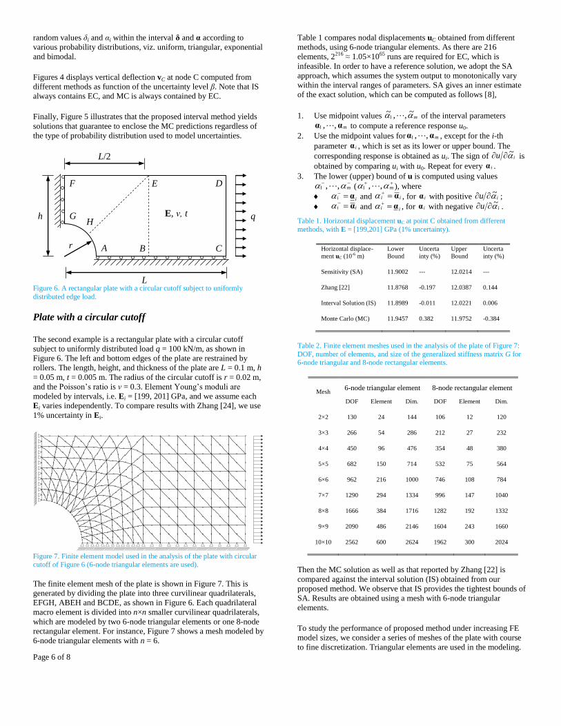
Figure 6. A rectangular plate with a circular cutoff subject to uniformly

distributed edge load.

Plate with a circular cutoff

The second example is a rectangular plate with a circular cutoff

subject to uniformly distributed load q = 100 kN/m, as shown in

Figure 6. The left and bottom edges of the plate are restrained by

rollers. The length, height, and thickness of the plate are L = 0.1 m, h

= 0.05 m, t = 0.005 m. The radius of the circular cutoff is r = 0.02 m,

and the Poisson’s ratio is ν = 0.3. Element Young’s moduli are

modeled by intervals, i.e. Ei = [199, 201] GPa, and we assume each

Ei varies independently. To compare results with Zhang [24], we use

1% uncertainty in Ei.

Figure 7. Finite element model used in the analysis of the plate with circular cutoff of Figure 6 (6-node triangular elements are used).

The finite element mesh of the plate is shown in Figure 7. This is

generated by dividing the plate into three curvilinear quadrilaterals,

EFGH, ABEH and BCDE, as shown in Figure 6. Each quadrilateral

macro element is divided into n×n smaller curvilinear quadrilaterals,

which are modeled by two 6-node triangular elements or one 8-node

rectangular element. For instance, Figure 7 shows a mesh modeled by

6-node triangular elements with n = 6.

Table 1 compares nodal displacements uC obtained from different

methods, using 6-node triangular elements. As there are 216

elements, 2216 ≈ 1.05×1065 runs are required for EC, which is

infeasible. In order to have a reference solution, we adopt the SA

approach, which assumes the system output to monotonically vary

within the interval ranges of parameters. SA gives an inner estimate

of the exact solution, which can be computed as follows [8],

1. Use midpoint values m ~ , ,~ of the interval parameters

mαα , , to compute a reference response u0.

2. Use the midpoint values for mαα , , , except for the i-th

parameter iα , which is set as its lower or upper bound. The

corresponding response is obtained as ui. The sign of iu ~ is

obtained by comparing ui with u0. Repeat for every iα .

3. The lower (upper) bound of u is computed using values

m , , (

m , , ), where

ii α and ii α , for iα with positive iu ~ ;

ii α and ii α , for iα with negative iu ~ .

Table 1. Horizontal displacement uC at point C obtained from different

methods, with E = [199,201] GPa (1% uncertainty).

Horizontal displace-

ment uC (10-6 m)

Lower

Bound

Uncerta

inty (%)

Upper

Bound

Uncerta

inty (%)

Sensitivity (SA) 11.9002 --- 12.0214 ---

Zhang [22] 11.8768 -0.197 12.0387 0.144

Interval Solution (IS) 11.8989 -0.011 12.0221 0.006

Monte Carlo (MC) 11.9457 0.382 11.9752 -0.384

Table 2. Finite element meshes used in the analysis of the plate of Figure 7:

DOF, number of elements, and size of the generalized stiffness matrix G for 6-node triangular and 8-node rectangular elements.

Mesh 6-node triangular element 8-node rectangular element

DOF Element Dim. DOF Element Dim.

2×2 130 24 144 106 12 120

3×3 266 54 286 212 27 232

4×4 450 96 476 354 48 380

5×5 682 150 714 532 75 564

6×6 962 216 1000 746 108 784

7×7 1290 294 1334 996 147 1040

8×8 1666 384 1716 1282 192 1332

9×9 2090 486 2146 1604 243 1660

10×10 2562 600 2624 1962 300 2024

Then the MC solution as well as that reported by Zhang [22] is

compared against the interval solution (IS) obtained from our

proposed method. We observe that IS provides the tightest bounds of

SA. Results are obtained using a mesh with 6-node triangular

elements.

To study the performance of proposed method under increasing FE

model sizes, we consider a series of meshes of the plate with course

to fine discretization. Triangular elements are used in the modeling.

Page 7 of 8

Table 2 lists the total DOF, element numbers and dimension of the

matrix G for each mesh. Here, 5% material uncertainty is considered

and Ei = [195, 205] GPa. Nodal displacements uC computed from

different methods are displayed in Figure 8. The SA solution is set as

a reference. This is compared against MC solution and the IS. SA and

MC can only be computed for coarse meshes.

Figure 8. Horizontal displacement uC at point C, obtained from different finite

element meshes, with E = [195,205] GPa (5% uncertainty).

From Figure 8, we observe the following: when the mesh is refined,

the overall widths of the interval solutions do not change, and the

difference between IS and SA remains unchanged. This means that

overestimation in our proposed method, if any, does not depend on

specific finite element mesh or problem scale.

Conclusions

We have proposed a new interval-based method for the analysis of

the extreme response of plane stress/strain problems, with

uncertainties in load, geometry and material. To reduce

overestimation in the solution, we have proposed a new

decomposition strategy for stiffness matrix (K), separating scalar

components from interval ones, thus limiting multiple occurrence of

the same interval variable. We solve primary and derived quantities

simultaneously using Lagrangian multipliers [20]. The interval

equilibrium equations are solved by means of a new variant of the

iterative enclosure method [18], which exploits the new

decomposition for K. Several numerical examples confirm that using

the proposed method supersedes all available interval methods in

literature [8, 17] by attaining the tightest guaranteed enclosures of the

structural extreme response. Furthermore, the proposed method

yields reliable solutions even under excessively large level of

uncertainties (30-40%). In addition, the computational time is

negligible if compared to the endpoint combination method,

sensitivity analysis, and Monte Carlo method.

References

1. Alefeld, G. and Herzberger, J., “Introduction to Interval

Computation”, Academic Press, San Diego, 1983.

2. Cook, R.D., Malkus, D.S., Plesha, M.E., Witt, R.J., “Concepts

and applications of finite element analysis”, John Wiley & Sons,

2007.

3. Corliss, G., Foley, C., Kearfott, R.B., “Formulation for Reliable

Analysis of Structural Frames”, Reliable Computing, 13(2): 125-

147, 2007.

4. Ellingwood, B.R. and Kinali, K., “Quantifying and

communicating uncertainty in seismic risk assessment”,

Structural Safety, 31:179–87, 2009.

5. Impollonia, N., “A method to derive approximate explicit

solutions for structural mechanics problems”, International

Journal of Solids and Structures, 43: 7082–7098, 2006.

6. Impollonia, N. and Muscolino, G., “Interval analysis of

structures with uncertain-but-bounded axial stiffness”, Comput.

Methods Appl. Mech. Engrg., 220(21-22): 1945-1962, 2011.

7. Jiang, C., Zhang, Z., Han, X., Liu, J., “A novel evidence-theory-

based reliability analysis method for structures with epistemic

uncertainty”, Computers and Structures, 129: 1–12, 2013.

8. Kreinovich, V., Beck, J., Ferregut, C., Sanchez, A., et al.,

“Monte-carlo-type techniques for processing interval

uncertainty, and their engineering applications”, Proc. NSF

workshop on reliable engineering computing, R. L. Muhanna

and R. L. Mullen, eds., Savannah, GA, 2004.

http://www.gtsav.gatech.edu/rec/recworkshop/index.html.

9. Kulisch, U.W. and Miranker, W.L., “Computer Arithmetic in

Theory and Practice”, Academic Press, New York, 1981.

10. Lutes, L.D. and Sarkani, S., “Random Vibrations”, edited by

Loren D. Lutes and Shahram Sarkani, Butterworth-Heinemann,

Burlington, 2004.

11. Moens, D. and Vandepitte, D., “A survey of non-probabilistic

uncertainty treatment in finite element analysis”, Comput.

Methods Appl. Mech. Engrg., 194: 1527–1555, 2005.

12. Moore, R.E., Kearfott, R.B., Cloud M.J., “Introduction to

interval analysis”, Society for Industrial and Applied

Mathematics, Philadelphia, 2009.

13. Muhanna, R.L. and Mullen, R.L., “Formulation of Fuzzy Finite-

Element Methods for Solid Mechanics Problems”, Computer-

Aided Civil and Infrastructure Engineering, 14: 107–117, 1999.

14. Muhanna, R.L. and Mullen, R.L., “Uncertainty in Mechanics

Problems - Interval-Based Approach”, Journal of Engineering

Mechanics ASCE, 127(6): 557-566, 2001.

15. Muhanna, R.L., Zhang, H., Mullen, R.L., “Combined Axial and

Bending Stiffness in Interval Finite-Element Methods”, Journal

of Structural Engineering, 133(12): 1700–1709, 2007.

16. Mullen, R. L. and Muhanna, R. L., “Bounds of Structural

Response for All Possible Loadings”, Journal of Structural

Engineering, 125(1): 98-106, 1999.

17. Neumaier, A., “Interval methods for systems of equations”,

Cambridge University Press, New York, 1990.

18. Neumaier, A. and Pownuk, A., “Linear systems with large

uncertainties, with applications to truss structures”, Reliable

Computing, 13(2): 149–172, 2007.

19. Pownuk, A., “Calculation of the extreme values of

displacements in truss structures with interval parameters”,

2004. Available online at:

http://andrzej.pownuk.com/php/ansys2interval/

20. Rama Rao, M.V., Mullen, R.L., Muhanna, R.L., “A New

Interval Finite Element Formulation with the same accuracy in

primary and derived variables”, Int. J. Reliability and Safety, 5

(3/4): 336-367, 2011.

21. Rump, S.M., “INTLAB - INTerval LABoratory”, In T. Csendes

(eds), editor, Developments in Reliable Computing: 77-104.

Dordrecht: Kluwer Academic Publishers, 1999.

http://www.ti3.tu-harburg.de/rump/intlab/

22. Zhang, H., “Nondeterministic Linear Static Finite Element

Analysis: An Interval Approach”, PhD Dissertation. School of

Civil and Environmental Engineering, Georgia Institute of

Technology, Atlanta, GA. 2005.

23. Dempster, A.P., “Upper and lower probabilities induced by a

muilti-valued mapping”, Ann. Math. Stat., 38: 325–339, 1967.

24. Shafer, G., “A mathematical theory of evidence”. Princeton

University Press, Princeton, 1968.

Page 8 of 8

25. Adhikari, S. and Khodaparast, H. H., “A spectral approach for

fuzzy uncertainty propagation in finite element analysis”, Fuzzy

Sets and Systems, 243: 1–24, 2014.

26. Klir, G.J. and Wierman, M.J., “Uncertainty-based information -

Elements of generalized information theory”, Physica-Verlag,

Heidelberg, 1999.

27. Sim, J., Qiu, Z., and Wang, X., “Modal analysis of structures

with uncertain-but-bounded parameters via interval analysis”,

Journal of Sound and Vibration, 303: 29–45, 2007.

28. Yang, Y., Cai, Z., and Liu, Y., “Interval analysis of frequency

response functions of structures with uncertain parameters”,

Mechanics Research Communications, 47: 24–31, 2013.

29. Bathe, K. and Wilson, E.L., “Numerical methods in finite

element analysis”, Prentice-Hall, Inc., Englewood Cliffs, New

Jersey, 1976.