COMPREHENSIVE ANALYSIS OF ACID STIMULATION IN CARBONATES

A Dissertation

by

MATEUS PALHARINI SCHWALBERT

Submitted to the Office of Graduate and Professional Studies of Texas A&M University

in partial fulfillment of the requirements for the degree of

DOCTOR OF PHILOSOPHY

Chair of Committee, Ding Zhu Co-Chair of Committee, Alfred Daniel Hill Committee Members, Eduardo Gildin

Victor Ugaz Head of Department, Jeff Spath

August 2019

Major Subject: Petroleum Engineering

Copyright 2019 Mateus Palharini Schwalbert

ii

ABSTRACT

Most wells in conventional carbonate reservoirs are stimulated with acid, either by

acid fracturing or by matrix acidizing. Both methods can result in effective stimulation in

carbonate reservoirs, but currently there is no published scientific criterion for selecting

one technique or the other. The objectives of this study are to define ways to estimate the

well performance that can be obtained from each of these treatments, and finally to define

a decision criterion to select the best acid stimulation technique for a given scenario.

Improvements in the modeling of both matrix acidizing and acid fracturing are

proposed in this study. A new upscaled global model of wormhole propagation is

proposed, based on experimental results and simulations using the Two-Scale Continuum

Model. The proposed model represents experiments in different scales and field

treatments. The wormhole propagation in anisotropic formations and in limited entry

completions was also studied, and new analytical equations to calculate the post-acidizing

skin factor for these cases were presented.

In terms of acid fracturing modeling, a productivity model was developed for acid

fractures, coupled to an in-house acid fracturing simulator. A leak-off model accounting

for efficient wormholing was also developed, improving the prediction of high leakoff

observed in acid fracturing treatments.

Comparing the predicted productivity of matrix acidized and acid fractured wells,

this study proposes a criterion for selection of the acid stimulation technique that results

in the most productive well, for a given scenario and volume of acid. For all scenarios

iii

studied, there is a cutoff permeability above which a matrix acidized well is more

productive than an acid fractured well. The value of this cutoff permeability, however,

changes significantly for different scenarios. For example, in shallower reservoirs with

small horizontal stresses, the cutoff permeability is much higher than in deeper reservoirs

subject to high horizontal stresses. For hard rocks, the cutoff permeability is higher than

for softer rocks.

Concise analytical decision criteria were proposed to select the best acid

stimulation method for both vertical and horizontal wells.

iv

DEDICATION

To my amazing family, especially Aline, Fox, and Scully.

v

ACKNOWLEDGEMENTS

I would like express my sincere gratitude to Dr. Ding Zhu and Dr. Dan Hill for

adopting me into this research group and providing guidance, knowledge, and support

throughout these years. We had valuable discussions and I learned a lot from both.

I would like to thank Dr. Eduardo Gildin and Dr. Victor Ugaz for serving as my

committee members and expressing interest in my research.

I would like to thank also all my colleagues from the research group, especially to

Dr. Murtada Al Jawad, who developed the fully-coupled acid fracturing model used as a

basis to part of this research. We spent many hours across many months discussing this

model and joining efforts to make it right and useful. Special thanks also go to Robert

Shirley for many enjoyable discussions.

I must thank twice Dr. Ding Zhu for the opportunity to serve as a Graduate

Teaching Fellow and teach one of her courses. It was a great experience that will definitely

shape my career. I thank also Dr. Iberê Alves for all the valuable discussion and help

during this enterprise.

These years would not have been so enjoyable without the many friends I made in

Texas. Thanks also go to you guys. Although the BBB College Station is approaching an

end, we will see each other around. Thanks also to John Muir and Theodore Roosevelt for

making my life in this country so enjoyable.

Finally, thanks to my family for their encouragement and support. Especially to

my wife, the best person in the world, whose patience and love are unending.

vi

CONTRIBUTORS AND FUNDING SOURCES

This work was supervised by a dissertation committee consisting of Dr. Ding Zhu

(committee chair), Dr. Dan Hill (co-chair), and Dr. Eduardo Gildin of the Department of

Petroleum Engineering, and Dr. Victor Ugaz of the Department of Chemical Engineering.

The fully-coupled acid fracturing simulator presented in section 4.2 was developed

by Murtada Al Jawad and published in 2018, except for the modifications mentioned in

this text and the productivity model. The CT-scans in Figure 3-15 were provided by Robert

Shirley.

This research was financially supported by Petrobras. The contents are solely the

responsibility of the author and do not necessarily represent the official views of Petrobras.

Portions of this research were conducted with High Performance Research

Computing resources provided by Texas A&M University (https://hprc.tamu.edu).

vii

NOMENCLATURE

𝐴 = (1) Parameter of generalized acid fracture conductivity correlation

𝐴 = (2) Cross sectional area perpendicular to the wormhole front

𝐴 = (3) Surface area

𝐴 = Reservoir drainage area of a given well

𝐴 = Wellbore surface area

𝑎 = Drainage region length in the direction orthogonal to horizontal

well

𝑎 = Magnitude of permeability heterogeneity in the uniform random

distribution

𝑎 = Mineral specific surface area

𝑎 = Initial mineral specific surface area

𝑎 = Magnitude of porosity heterogeneity in the uniform random

distribution

𝐵 = (1) Parameter of generalized acid fracture conductivity correlation

𝐵 = (2) Formation volume factor

𝑏 = Parameter in Sherwood number correlation

𝐶 = Acid concentration

𝐶 = Concentration of the injected acid

𝐶 = Concentration of the leaking acid

viii

𝐶 = Bulk acid concentration

𝐶 = Leakoff coefficient component due to reservoir fluids compression

𝐶 , = Leakoff coefficient component due to reservoir fluids compression with

wormholes

𝐶 = Acid concentration at the reaction equilibrium

𝐶 = (1) Acid concentration (mass fraction) in the bulk fluid

𝐶 = (2) Fracture conductivity

𝐶 = Dimensionless fracture conductivity

𝐶 , = Optimal dimensionless fracture conductivity

𝐶 = Injected acid concentration (mass fraction)

𝐶 = Leakoff coefficient

𝐶 = Leakoff coefficient of fluid 1

𝐶 = Leakoff coefficient of fluid 2

𝐶 = Heat capacity

𝐶 = (1) Acid concentration (mass fraction) in the solid-fluid interface

𝐶 = (2) Stimulation coverage, in a well acidized with limited entry

technique

𝐶 = Leakoff coefficient component due to viscous filtrate invasion

𝐶 , = Leakoff coefficient component of wormholed invaded zone, in the model

by Hill et al. (1995)

𝐶 = (1) Leakoff coefficient component due wall-building filter cake

ix

𝐶 = (2) Acid concentration at the fracture wall

𝑐 = Total formation compressibility

𝐷 = Acid species diffusivity coefficient

𝐷 = Effective diffusivity coefficient

𝐷 = Molecular diffusivity coefficient

𝑑 = General linear dimension, such as a diameter, or a general “scale”

𝑑 = Core diameter

𝑑 , = Equivalent wormhole cluster diameter, parameter in the model by

Furui et al. (2010)

𝑑 = Fractal dimension

𝑑 , = Parameter of the proposed wormhole global model; representative

scale up to which there is decrease in 𝑃𝑉 ,

𝑑 , = Parameter of the proposed wormhole global model; representative

scale up to which there is decrease in 𝑣 ,

𝑑 = Scale related to the decrease in 𝑃𝑉 ,

𝑑 = Scale related to the decrease in 𝑣 ,

𝑓 = Fraction of injected acid spent etching the fracture walls

𝑓 = Number between 0 and 1, assumption as to how much of the bulk acid

concentration leaks

𝑔(𝜆) = Function of the aspect ratio in Meyer and Jacot (2005) model

𝒈 = Gravity acceleration vector

x

ℎ = Reservoir thickness, net pay

ℎ = Fracture height

ℎ = Perforation spacing, the inverse of the perforation density; the

spacing between acid injection points in a limited entry scheme

∆𝐻 = Heat of reaction

𝐼 = Reservoir anisotropy ratio

𝐼 , = Wormhole anisotropy ratio, 𝑟 /𝑟

𝐼 = Fracture penetration ratio, 𝐼 = 2𝑥 /𝑥

𝐽 = Productivity or injectivity index

𝐽 = Dimensionless productivity index

𝐽 , , = Maximum 𝐽 achievable with acid fracturing

𝐽 , , = Maximum 𝐽 achievable with matrix acidizing

𝐽 , = Maximum possible dimensionless productivity index

𝐽 , = 𝐽 of a horizontal acid fractured well

𝐽 , = 𝐽 of a horizontal matrix acidized well

𝐽 = Flux of acid transported by mass transfer

𝑘 = Permeability (scalar)

𝒌 = Permeability tensor

𝒌 = Mean permeability tensor

𝒌𝒐 = Initial permeability tensor

𝑘 = geometric mean of permeability in elliptical flow

xi

𝑘 = Mass transfer coefficient

𝑘 = Cutoff permeability, above which matrix acidizing can result in a

higher productivity index than acid fracturing

𝑘 = Effective mass transfer coefficient, including reaction and mass

transfer effects

𝑘 𝑤 = Fracture conductivity

𝑘 𝑤 = Fracture conductivity at the wellbore-fracture contact

𝑘 = Horizontal permeability

𝑘 = Mean horizontal permeability

𝑘 = Mean permeability value in the direction of maximum permeability

𝑘 = Reaction rate pre-exponential coefficient

𝑘 = Surface reaction rate “constant”

𝑘 = spherical permeability, or equivalent permeability in spherical flow

𝑘 = Vertical permeability

𝑘 = Mean vertical permeability

𝑘 = Permeability of wormholed region (usually regarded as infinite)

𝐿 = Wellbore length

𝐿 , = Parameter of the proposed wormhole global model; representative

length up to which there is decrease in 𝑃𝑉 , in radial geometry

𝐿 , = Parameter of the proposed wormhole global model; representative

length up to which there is decrease in 𝑣 , in radial geometry

xii

𝑙 = Perforation length

𝑙 = Wormhole length in a linear geometry

𝑚 = Mass of acid spent etching the fracture walls

𝑚 = Mass of acid injected

𝑚 = Mass of acid lost due to leakoff

𝑚 = Number of wormholes in a 2D plane, parameter in the model by

Furui et al. (2010)

𝑁 = Acid capacity number

𝑁 = Carbonate acid stimulation number; if 𝑁 > 1, acid fracturing is

preferable over matrix acidizing

𝑁 = Number of transverse fractures in a horizontal well

𝑁 = Number of leakoff with wormholes

𝑁 = Proppant number (dimensionless)

𝑛 = Reaction rate order

𝒏𝒘 = Unit normal vector at the wellbore

𝑃𝐼𝑅 = Productivity index ratio between acid fractured and matrix acidized

wells

𝑃𝑉 = Pore volumes to breakthrough, in wormhole propagation

𝑃𝑉 , = Representative value of 𝑃𝑉 for a given field

𝑃𝑉 , = Minimum value of 𝑃𝑉 , in the field scale

𝑃𝑉 , = Optimum pore volumes to breakthrough, in wormhole propagation

xiii

𝑃𝑉 , , = Optimum pore volumes to breakthrough measured with cores of

diameter 𝑑

𝑃𝑉 , , = Optimum pore volumes to breakthrough measured with cores of

diameter 𝑑

𝑃𝑉 , , = Optimum pore volumes to breakthrough in the core scale, in

wormhole propagation

𝑃𝑉 , , = Minimum value for the optimum pore volumes to breakthrough,

reached at a large enough scale

𝑝 = Pressure

𝑝 = Pressure inside the fracture

𝑝 = Initial reservoir pressure

𝑝 = Wellbore pressure

𝑝 , = Initial wellbore pressure

𝑝 , = Pressure at the tip of the wormhole front

𝑝 , = Pressure pre-existent (from previous time step) at the wormhole front

∆𝑝 = Pressure drop in region of ellipsoidal flow

∆𝑝 = Pressure drop in region of elliptical flow

∆𝑝 = Pressure drop in region of linear flow

∆𝑝 = Pressure drop in region of radial flow

∆𝑝 = Pressure drop in region of spherical flow

𝑞 = Flow rate (injection or production rate)

xiv

𝑞 = Production rate from each perforation in a limited entry scheme

𝑞 = Heat flux from the reservoir in the heat transfer analysis

𝑅(𝐶 ) = Acid-mineral surface reaction rate

𝑅 = Dimensionless square of the ratio between 𝐶 and 𝐶

𝑅𝑒 = Pore scale Reynolds number

𝑅 = Radius of the wormholed region in a spherical wormhole

propagation

𝑅 = Horizontal length of ellipsoidal wormhole network, or horizontal

semi-axis of ellipsoidal wormhole network

𝑅 = Vertical length of ellipsoidal wormhole network, or vertical semi-

axis of ellipsoidal wormhole network

𝑅 , , = Parameter of the proposed wormhole model in spherical geometry;

representative radius of the wormholed region up to which there is

decrease in 𝑃𝑉 ,

𝑅 , , = Parameter of the proposed wormhole model in spherical geometry;

representative radius of the wormholed region up to which there is

decrease in 𝑣 ,

𝑟 = External radius of a drainage region

𝑟 = Standard normally distributed random number

𝑟 = Representative pore radius

𝑟 = Initial representative pore radius

xv

𝑟 = Uniformly distributed random number between 0 and 1

𝑟 = wellbore radius

𝑟 = Equivalent wellbore radius

𝑟 = Radius of cylindrical wormholed region

𝑟 = Horizontal length of wormhole network, or horizontal semi-axis of

elliptical wormhole network

𝑟∗ = Horizontal length of wormhole network after the different

stimulated regions interconnect

𝑟 = Vertical length of wormhole network, or vertical semi-axis of

elliptical wormhole network

𝑟 , , = Parameter of the proposed wormhole global model; representative

radius of the wormholed region up to which there is decrease in

𝑃𝑉 , in radial geometry

𝑟 , , = Parameter of the proposed wormhole global model; representative

radius of the wormholed region up to which there is decrease in

𝑣 , in radial geometry

𝑆𝑐 = Schmidt number

𝑆ℎ = Sherwood number

𝑆ℎ = Asymptotic Sherwood number

𝑠 = Skin factor

𝑠 = Choke skin factor in a transverse fracture (horizontal well)

xvi

𝑠 = Skin factor of the matrix acidized well

𝑇 = Temperature

𝑡 = Time

𝑈 = Superficial or Darcy velocity

𝑈 = Injected acid velocity at the inlet

𝑉 = Total acid volume injected

𝑉 = Acid volume spent etching the acid fracture walls

𝑉 = Reservoir drainage volume of a given well

𝑉 = Etched volume (volume of rock dissolved by acid on fracture

faces)

𝑉 , = Maximum possible etched volume

𝑉 = Volume of the propped fracture in the pay zone

𝑉 = Stimulated volume.

(𝑉 ) = volume of acid required for the optimal stimulation coverage, in

anisotropic wormhole propagation

(𝑉 ) = volume of acid required for the optimal stimulation coverage, in

isotropic wormhole propagation

𝑣 = Interstitial velocity

�̅� = Average interstitial velocity at the wormhole front

𝑣 , = Optimal interstitial velocity, in wormhole propagation

𝑣 , , = Optimal interstitial velocity measured with cores of diameter 𝑑

xvii

𝑣 , , = Optimal interstitial velocity measured with cores of diameter 𝑑

𝑣 = Leakoff velocity

𝑣 = Velocity of propagation of the wormhole front

𝑤 = Fracture width

𝑤 = Fracture etched width (ideal width dissolved by acid)

𝑤 , = Etched width corrected by the maximum possible etched volume

𝑥 = Horizontal direction; direction of the fracture in a fractured vertical

well; direction of the wellbore in a horizontal well

𝑥 = Drainage region length in x-direction

𝑥 = Fracture half-length

𝑥 = Fracture half-length occupied by fluid 1, when multiple fluids are

used

𝑥 , = Fracture half-length occupied by the acid system

𝑥 , = Optimal fracture half-length

𝑥 , = Fracture half-length occupied by the pad

𝑦 = Distance orthogonal to fracture walls (for vertical wells)

𝑦 = Half the distance from a horizontal well to the boundary in the

direction orthogonal to the well, or half the well spacing

𝑦 = Drainage region length in y-direction

xviii

Greek

𝛼 = Exponent relating wormhole growth with time (𝑟 ∝ 𝑡 )

𝛼 = Parameter in the model by Furui et al. (2010)

𝛽 = Acid gravimetric dissolving power (of the pure, 100% acid)

𝛾 = (1) Parameter of the pore radius evolution model

𝛾 = (2) Parameter in the models by Buijse and Glasbergen (2005),

Furui et al. (2010), and this work; commonly regarded as 1/3

𝛾 = (3) Euler-Mascheroni constant (𝑒 ≈ 1.781)

𝛿 = Parameter of the permeability evolution model

𝜀 = Parameter of the proposed wormhole model; exponent relating

decrease in 𝑃𝑉 , as the scale increases

𝜀 = Parameter of the proposed wormhole model; exponent relating

decrease in 𝑣 , as the scale increases

𝜂 = Parameter of the specific surface area evolution model

𝜅 = Thermal conductivity

𝜆 = Aspect ratio of the drainage region, 𝜆 = 𝑥 /𝑦

𝜆 = Permeability correlation length in horizontal direction

𝜆 = Permeability correlation length in vertical direction

𝜆 = Permeability correlation length in x-direction

𝜆 = Permeability correlation length in y-direction

𝜌 = Acid solution density

xix

𝜌 = Fluid density

𝜌 = Mineral density

𝜎 = Effective confining stress

𝜎 , = Minimum horizontal stress

𝜎 = Standard deviation of the natural logarithm of permeability in log-

normal distribution

𝜇 = Fluid dynamic viscosity

𝜇 = Viscosity of the filtrate flowing in the invaded zone

𝜇 = Viscosity of the fluid in the wormholed region

𝜙 = Rock porosity

𝜙 = Rock mean porosity

𝜙 = Rock initial porosity

𝜁 = Ratio 𝑥 /𝑟 for a fracture of infinite conductivity

xx

TABLE OF CONTENTS

Page

ABSTRACT .......................................................................................................................ii

DEDICATION .................................................................................................................. iv

ACKNOWLEDGEMENTS ............................................................................................... v

CONTRIBUTORS AND FUNDING SOURCES ............................................................. vi

NOMENCLATURE .........................................................................................................vii

TABLE OF CONTENTS ................................................................................................. xx

LIST OF FIGURES ...................................................................................................... xxiii

LIST OF TABLES .......................................................................................................xxxi

1. INTRODUCTION .......................................................................................................... 1

1.1. Carbonate Matrix Acidizing .................................................................................... 1 1.2. Acid Fracturing ....................................................................................................... 3 1.3. Propped Hydraulic Fracturing ................................................................................. 4 1.4. Comparison of the Stimulation Methods ................................................................ 5

2. LITERATURE REVIEW .............................................................................................. 7

2.1. Oil Well Performance.............................................................................................. 8 2.2. Carbonate Matrix Acidizing .................................................................................. 10

2.2.1. Models to Find the Optimal Matrix Acidizing Condition .............................. 16 2.2.2. Global Models of Wormhole Propagation ..................................................... 23 2.2.3. Performance Estimate for Matrix Acidized Wells ......................................... 29

2.3. Acid Fracturing ..................................................................................................... 36 2.3.1. Acid Fracture Models ..................................................................................... 37 2.3.2. Acid Leakoff from Acid Fractures ................................................................. 40 2.3.3. Acid Fracture Conductivity ............................................................................ 43 2.3.4. Acid Fractured Well Performance .................................................................. 45

2.4. Stimulation Method Selection ............................................................................... 47 2.5. Research Objectives .............................................................................................. 50

3. IMPROVEMENTS IN MATRIX ACIDIZING MODELING ................................... 52

xxi

3.1. Two-Scale Continuum Model ............................................................................... 52 3.1.1. Mathematical Model ....................................................................................... 54 3.1.2. Validation of the Model - Experimental Data Matching ................................ 68 3.1.3. Simulation of 2D Radial Wormhole Propagation .......................................... 75 3.1.4. Simulation of Spherical Wormhole Propagation ............................................ 89 3.1.5. Large Scale 3D Simulations ........................................................................... 95

3.2. New Upscaled Global Model for Wormhole Propagation .................................. 100 3.2.1. Corrections for the core diameter ................................................................. 101 3.2.2. New Proposed Global Wormhole Model ..................................................... 108 3.2.3. Validation of the Model ............................................................................... 117 3.2.4. Field Application .......................................................................................... 126

3.3. New Skin Factor Equations for Anisotropic Carbonates and Limited Entry Completions ............................................................................................................... 131

3.3.1. Impact of Anisotropic Wormhole Networks on Productivity ...................... 135 3.3.2. Wormhole Coverage to Avoid Partial Completion in the Limited Entry ..... 144 3.3.3. Equations for the Skin Factor of Anisotropic Wormhole Networks ............ 152

3.4. Estimating the Productivity of Matrix Acidized Wells ....................................... 164 3.4.1. Theoretical Maximum Productivity of Matrix Acidized Wells ................... 174

4. IMPROVEMENTS IN ACID FRACTURING MODELING .................................. 179

4.1. New Acid Leakoff Model for Acid Fracturing ................................................... 179 4.1.1. Derivation of the New Leakoff Model ......................................................... 182 4.1.2. Validation of the New Leakoff Model ......................................................... 195 4.1.3. Dimensional Analysis of the Wormhole Effect on Leakoff ......................... 198

4.2. Fully-Coupled Acid Fracturing Model ................................................................ 206 4.2.1. Modifications on the Acid Fracturing Model ............................................... 214

4.3. Productivity Model for Acid Fractured Wells..................................................... 219 4.3.1. Validation of the Productivity Model ........................................................... 225 4.3.2. Wormholes in the Productivity Model ......................................................... 227

4.4. Acid Fracturing Design and Maximum Productivity Estimation ........................ 229 4.5. Analytical Estimate of Maximum Possible Acid Fractured Well Productivity .. 240

5. ACID STIMULATION METHOD SELECTION FOR CARBONATES ................ 262

5.1. Case Studies – Comparison Between Matrix Acidizing and Acid Fracturing .... 266 5.1.1. Scenario 1 – base case .................................................................................. 266 5.1.2. Scenario 2 – shallow reservoir ..................................................................... 268 5.1.3. Scenario 3 – deep reservoir .......................................................................... 269 5.1.4. Scenarios 1S, 2S, and 3S – soft limestones .................................................. 270 5.1.5. Scenarios 1H, 2H, and 3H – hard limestones ............................................... 273 5.1.6. Scenarios 4 and 5 – different acid volumes .................................................. 276 5.1.7. Scenario 6 – injector well ............................................................................. 280 5.1.8. Impact of the wormhole model .................................................................... 282

xxii

5.1.9. Scenario 9 – dolomite formation .................................................................. 285 5.1.10. Summary of the Case Studies for Vertical Wells ....................................... 290

5.2. Concise Decision Criterion for Vertical Wells ................................................... 291 5.3. Concise Decision Criterion for Horizontal Wells ............................................... 298

5.3.1. Scenario 10 – horizontal well ....................................................................... 303 5.3.2. Scenario 11 – larger acid volume ................................................................. 308 5.3.3. Soft chalks .................................................................................................... 311

6. CONCLUSIONS ........................................................................................................ 317

REFERENCES ............................................................................................................... 323

APPENDIX A ............................................................................................................... 338

APPENDIX B ............................................................................................................... 342

APPENDIX C ............................................................................................................... 345

APPENDIX D ............................................................................................................... 349

APPENDIX E ................................................................................................................ 352

APPENDIX F ................................................................................................................ 358

APPENDIX G ............................................................................................................... 365

APPENDIX H ............................................................................................................... 369

APPENDIX I .................................................................................................................. 371

I.1 Nierode and Kruk (1973) correlation .................................................................... 371 I.2 Deng et al. (2012) correlation ............................................................................... 372

I.2.1 Permeability-Distribution-Dominant Cases with High Leakoff .................... 373 I.2.2 Permeability-Distribution-Dominant Cases with Medium Leakoff ............... 374 I.2.3 Mineralogy-Distribution-Dominant Cases ..................................................... 374 I.2.4 Competing Effects of Permeability and Mineralogy Distributions ............... 375

I.3 Neumann (2011) correlation ................................................................................. 376 I.4 Nasr-El-Din et al. (2008) correlations .................................................................. 376

xxiii

LIST OF FIGURES

Page

Figure 1-1: CT-scan images of wormholed blocks of carbonates. ..................................... 2

Figure 1-2: illustration of the acid fracturing operation. .................................................... 3

Figure 1-3: acid-etched fracture from a laboratory experiment. ........................................ 4

Figure 2-1: neutron radiographs of dissolution patterns obtained by injecting HCl into chalk at different injection rates. ............................................................... 13

Figure 2-2: “acid” efficiency curves for different acids and chelating agents. ................ 14

Figure 2-3: Position of each dissolution pattern and on the acid efficiency curve. ......... 15

Figure 2-4: Collection of published data of 𝑷𝑽𝒃𝒕, 𝒐𝒑𝒕 and 𝒗𝒊, 𝒐𝒑𝒕 comparing different core sizes. ........................................................................................... 21

Figure 2-5: Comparison of pore volumes to breakthrough (𝑷𝑽𝒃𝒕) for different laboratory scales and field treatments. .............................................................. 23

Figure 2-6: example of permeability profile in a carbonate reservoir. ............................. 31

Figure 2-7: Spherical stimulated regions arising from limited entry technique. .............. 36

Figure 2-8: example of acid fracturing treatment presenting premature fracture closure while pumping the acid. ....................................................................... 42

Figure 2-9: decision tree for stimulation method selection. ............................................. 48

Figure 3-1: Flowchart diagram illustrating the simulation sequence. .............................. 65

Figure 3-2: Example of simulation domain for the 1-in x 6-in core. (a) Grid; (b) Lognormal permeability field. .......................................................................... 69

Figure 3-3: Model tuning with experimental data from Furui et al. (2012a). .................. 70

Figure 3-4: Dissolution patterns for the points in Figure 3-3. (a) face dissolution, (b) conical wormhole, (c) dominant wormhole, and (d) uniform dissolution. ........................................................................................................ 72

xxiv

Figure 3-5: Example of simulation domain for the radial propagation. (a) Whole domain; (b) detail of the mesh; (c) lognormal permeability field; (d) detail of the lognormal permeability field ........................................................ 76

Figure 3-6: Initial condition for acid concentration. (a) Whole domain; (b) detail of the inlet. ........................................................................................................ 77

Figure 3-7: Example of the radial pressure field that develops with injection................. 78

Figure 3-8: example of radial propagation of wormholes in isotropic formations. Plots of (a) acid concentration, (b) porosity, and (c) superficial velocity magnitude. ........................................................................................................ 79

Figure 3-9: example of radial propagation of wormholes in isotropic formations in the whole 360o domain. Plots of (a) acid concentration, and (b) acid velocity. ............................................................................................................ 80

Figure 3-10: comparison of (a) simulation result from this work to (b) a real CT-scan image. ....................................................................................................... 81

Figure 3-11: simulation results for anisotropic rocks, with 𝒌𝑯 = 𝟏𝟎𝒌𝑽, where anisotropic wormhole distribution is observed. (a) 𝑼𝒊𝒏𝒍𝒆𝒕 =𝟏𝟎𝟎𝒄𝒎/𝒎𝒊𝒏, 𝝈𝒌 = 𝟎. 𝟐. (b) 𝑼𝒊𝒏𝒍𝒆𝒕 = 𝟐𝟎𝟎𝒄𝒎/𝒎𝒊𝒏, 𝝈𝒌 = 𝟎. 𝟐. (c) 𝑼𝒊𝒏𝒍𝒆𝒕 = 𝟐𝟎𝟎𝒄𝒎/𝒎𝒊𝒏, 𝝈𝒌 = 𝟎. 𝟒. (d) Illustration of the elliptical stimulated region. ............................................................................................. 83

Figure 3-12: simulation results for anisotropic rocks, with 𝒌𝑯 = 𝟏𝟎𝒌𝑽, where the wormhole distribution does not follow the permeability anisotropy. (a) 𝑼𝒊𝒏𝒍𝒆𝒕 = 𝟐𝟎𝒄𝒎/𝒎𝒊𝒏, 𝝈𝒌 = 𝟏. 𝟐. (b) 𝑼𝒊𝒏𝒍𝒆𝒕 = 𝟒𝟎𝒄𝒎/𝒎𝒊𝒏, 𝝈𝒌 =𝟎. 𝟖. ................................................................................................................... 84

Figure 3-13: permeability distributions showing different correlation lengths in horizontal and vertical directions. (a) 𝝀𝒙 = 𝝀𝒚, (b) 𝝀𝒙 = 𝟑𝝀𝒚, (c) 𝝀𝒙 =𝟓𝝀𝒚, and (d) 𝝀𝒙 = 𝟏𝟎𝝀𝒚. ................................................................................. 86

Figure 3-14: wormhole distributions obtained in the simulations with permeability distributions showing different correlation lengths in horizontal and vertical directions. (a) 𝝀𝒙 = 𝝀𝒚, (b) 𝝀𝒙 = 𝟑𝝀𝒚, (c) 𝝀𝒙 = 𝟓𝝀𝒚, and (d) 𝝀𝒙 = 𝟏𝟎𝝀𝒚. ...................................................................................................... 87

Figure 3-15: CT scans cores with wormholes aligned with the original rock laminations ........................................................................................................ 88

Figure 3-16: Simulation of linear core flooding in cores with inclined porosity laminations. ....................................................................................................... 89

xxv

Figure 3-17: Example of simulation domain for the spherical wormhole propagation. (a) Whole domain and mesh; (b) detail of the mesh; (c) lognormal permeability field; (d) detail of the acid inlet. ................................. 90

Figure 3-18: Simulation results of the spherical wormhole propagation for an isotropic formation. (a) Wormholes only; (b) wormhole network inside the simulation grid. ........................................................................................... 92

Figure 3-19: results of the simulation of the ellipsoidal wormhole network developed from acid injection in an anisotropic carbonate rock. (a) 𝑼𝒊𝒏𝒍𝒆𝒕 = 𝟐𝟎𝟎𝒄𝒎/𝒎𝒊𝒏, (b) 𝑼𝒊𝒏𝒍𝒆𝒕 = 𝟔𝟎𝟎𝒄𝒎/𝒎𝒊𝒏, (c) 𝑼𝒊𝒏𝒍𝒆𝒕 =𝟏𝟎𝟎𝟎𝒄𝒎/𝒎𝒊𝒏, (d) detail of the case (c) inside the simulation domain, showing the difference between vertical and horizontal wormhole propagation. ...................................................................................................... 94

Figure 3-20: Wormhole network obtained by simulating acid injection from a 𝟕𝟕𝟖 in. wellbore. .............................................................................................. 97

Figure 3-21: comparison of (a) 3D simulation result to (b) a real CT-scan image. ......... 98

Figure 3-22: simulation of wormhole propagation from a cased, cemented, and perforated wellbore. (a) wellbore with perforation; (b) wormhole network with a pressure contour. ...................................................................... 99

Figure 3-23: Match of proposed correlations (3.24) and (3.25) to published data. ....... 103

Figure 3-24: Plots of 𝑷𝑽𝒃𝒕, 𝒐𝒑𝒕 and 𝒗𝒊, 𝒐𝒑𝒕 versus the core diameter as obtained through numerical simulations using the Two-Scale Continuum Model. ...... 107

Figure 3-25: Comparison of the large scale simulations of the Two-Scale Continuum Model with the prediction of different global models of wormhole propagation. ................................................................................... 118

Figure 3-26: Comparison of the predictions of different wormhole global models for a synthetic case. ......................................................................................... 128

Figure 3-27: illustration of wormholed radius 𝒓𝒘𝒉 in a cylindrical stimulated region. ............................................................................................................. 133

Figure 3-28: Transverse cross sections of horizontal wells showing the stimulated region around the wellbore. (a) Anisotropic wormhole network; (b) isotropic wormhole network. .......................................................................... 136

Figure 3-29: Analysis of overestimation error caused by assuming a circular wormhole network instead of an elliptic wormhole network, in an

xxvi

openhole horizontal well. (a) Error for different reservoir anisotropy ratio, 𝑰𝒂𝒏𝒊. (b) Error for different wormhole radii. (c) Error for different well spacings. (d) Error for different formation thickness. ............................ 140

Figure 3-30: Illustration of anisotropic stimulated regions in wells acidized using limited entry technique. (a) Vertical well; (b) Horizontal well. ..................... 142

Figure 3-31: Overestimation error caused by assuming a spherical instead of an ellipsoidal wormhole network, as a function of anisotropy ratio. .................. 143

Figure 3-32: Sequence of time frames during wormhole propagation from a limited entry scheme. Results of simulations using the Two-Scale Continuum Model. (a) Porosity plots; (b) Pressure plots. .............................. 145

Figure 3-33: Sequence of time frames during wormhole propagation from a limited entry scheme. ...................................................................................... 146

Figure 3-34: Comparison of wormhole networks resulting from limited entry completions with different perforation densities but the same volume of acid. ................................................................................................................. 147

Figure 3-35: Skin factor versus stimulation coverage for the same stimulated volume per foot – vertical well ....................................................................... 148

Figure 3-36: Skin factor versus stimulation coverage for the same stimulated volume per foot – horizontal well ................................................................... 149

Figure 3-37: Comparison of flow rates resulting from a reservoir simulation and from the simple calculation with the proposed analytical equations for skin factor. ...................................................................................................... 160

Figure 3-38: example of field acid treatment data. ........................................................ 166

Figure 3-39: example of field acid treatment data. ........................................................ 167

Figure 3-40: example of synthetic matrix acidizing treatment, 10 md .......................... 170

Figure 3-41: example of synthetic matrix acidizing treatment, 60 md .......................... 171

Figure 3-42: comparison of the maximum and optimal injection rate for (a) 10 md and (b) 1 md .................................................................................................... 172

Figure 3-43: example dimensionless productivity index of matrix acidized wells ........ 173

Figure 4-1: pressure field in the reservoir due to leakoff without wormholes (the fracture face is located at y=0)........................................................................ 184

xxvii

Figure 4-2: pressure field in the reservoir due to leakoff with wormholes propagating (the fracture face is located at y=0). ........................................... 187

Figure 4-3: algorithm of new leakoff model with wormhole propagation. .................... 194

Figure 4-4: leakoff prediction in case of inefficient wormholing (𝑷𝑽𝒃𝒕, 𝒐𝒑𝒕 =𝟏𝟎𝟎𝟎) ............................................................................................................. 196

Figure 4-5: leakoff prediction in two cases of efficient wormholing. ............................ 197

Figure 4-6: Flowchart of the acid fracturing model ....................................................... 209

Figure 4-7: fracture geometry with 3 fluid systems ....................................................... 210

Figure 4-8: Results of an acid fracturing simulation with 2 fluid systems: pad + acid. (a) Fracture geometry, and (b) equivalent total leakoff coefficient ....... 211

Figure 4-9: example of fracture etched width and conductivity distribution obtained from an acid fracturing simulation. .................................................. 214

Figure 4-10: Diagram of the geometry of the fractured-well productivity model ......... 220

Figure 4-11: Example of x-y plane of the mesh used for the productivity model. ........ 221

Figure 4-12: Flowchart illustrating the proposed method for acid fracture productivity calculation. ................................................................................. 222

Figure 4-13: comparison of productivity numerical model with analytical solution. .... 226

Figure 4-14: comparison of acid fractured well productivity by including or not the wormholes in the productivity model ....................................................... 228

Figure 4-15: productivity index of well acid fractured with straight acid...................... 233

Figure 4-16: productivity index of well acid fractured with gelled acid. ....................... 233

Figure 4-17: productivity index of well acid fractured with emulsified acid. ................ 234

Figure 4-18: comparison of productivity index resulting from the three acid types ...... 236

Figure 4-19: comparison of productivity index for 100 bbl of acid ............................... 237

Figure 4-20: comparison of productivity index for 1,000 bbl of acid ............................ 237

Figure 4-21: maximum dimensionless productivity index for various acid volumes .... 238

xxviii

Figure 4-22: acid fractured well productivity for k = 0.01 md ...................................... 239

Figure 4-23: acid fractured well productivity for k = 1 md ........................................... 239

Figure 4-24: comparison of 𝑱𝑫, 𝒎𝒂𝒙 versus the acid volume, with the rough analytical estimate and the full simulation ..................................................... 255

Figure 4-25: comparison of 𝑱𝑫, 𝒎𝒂𝒙 versus reservoir permeability, with the rough analytical estimate and the full simulation ........................................... 257

Figure 4-26: comparison of the complete analytical equation (4.93) with the simplified analytical equation (4.82) and the full simulations ....................... 259

Figure 4-27: fraction of acid spent etching the fracture walls versus permeability ....... 261

Figure 5-1: comparison of matrix acidized and acid fractured well productivity – scenario 1, base case ....................................................................................... 267

Figure 5-2: comparison of matrix acidizing and acid fracturing – scenario 2, shallow reservoir ............................................................................................. 269

Figure 5-3: comparison of matrix acidizing and acid fracturing – scenario 3, deep reservoir .......................................................................................................... 270

Figure 5-4: comparison of matrix acidizing and acid fracturing – scenario 1S, soft limestone at medium depth ............................................................................. 271

Figure 5-5: comparison of matrix acidizing and acid fracturing – scenario 2S, shallow soft limestone .................................................................................... 272

Figure 5-6: comparison of matrix acidizing and acid fracturing – scenario 3S, deep soft limestone ......................................................................................... 272

Figure 5-7: comparison of matrix acidizing and acid fracturing – scenario 1H, hard limestone at medium depth ..................................................................... 274

Figure 5-8: comparison of matrix acidizing and acid fracturing – scenario 2H, shallow hard limestone ................................................................................... 274

Figure 5-9: comparison of matrix acidizing and acid fracturing – scenario 3H, deep hard limestone ........................................................................................ 275

Figure 5-10: comparison of different rock embedment strengths .................................. 276

Figure 5-11: impact of acid volume on (a) acid fracturing and (b) matrix acidizing ..... 277

xxix

Figure 5-12: comparison of matrix acidizing and acid fracturing – scenario 4, 100bbl of acid ................................................................................................. 278

Figure 5-13: comparison of matrix acidizing and acid fracturing – scenario 5, 2,000bbl of acid .............................................................................................. 278

Figure 5-14: comparison of matrix acidizing and acid fracturing – scenario 4S, soft rock and 100 bbl of acid .......................................................................... 279

Figure 5-15: comparison of matrix acidizing and acid fracturing – scenario 5S, soft rock and 2,000 bbl of acid ....................................................................... 280

Figure 5-16: comparison of matrix acidizing and acid fracturing – scenario 6, injector well .................................................................................................... 281

Figure 5-17: impact of the wormhole model on matrix acidized well productivity....... 283

Figure 5-18: comparison of matrix acidizing and acid fracturing – scenario 7, Buijse and Glasbergen’s model ...................................................................... 283

Figure 5-19: comparison of matrix acidizing and acid fracturing – scenario 8, Furui et al.’s model ......................................................................................... 284

Figure 5-20: comparison of acid stimulation outcomes in limestone and dolomite ...... 287

Figure 5-21: comparison of matrix acidizing and acid fracturing – scenario 9, dolomite .......................................................................................................... 287

Figure 5-22: optimal acid fracturing conditions for dolomite and limestone (1 md) ..... 288

Figure 5-23: (a) etched width and (b) conductivity profiles for dolomite and limestone ......................................................................................................... 289

Figure 5-24: comparison of the permeability cutoff estimated with analytical equation and resulting from full simulations .................................................. 297

Figure 5-25: dimensionless productivity index of the matrix acidized horizontal well ................................................................................................................. 304

Figure 5-26: dimensionless productivity index of the horizontal well with multiple acid fractures ................................................................................................... 305

Figure 5-27: comparison of matrix acidized and acid fractured horizontal well – scenario 10 ...................................................................................................... 306

xxx

Figure 5-28: comparison between matrix acidizing and acid fracturing for 2,000 ft by 5,000 ft drainage area; (a) matrix acidized well, (b) PI ratio. .................... 307

Figure 5-29: dimensionless productivity index of the matrix acidized horizontal well ................................................................................................................. 308

Figure 5-30: dimensionless productivity index of the horizontal well with multiple acid fractures ................................................................................................... 309

Figure 5-31: comparison of matrix acidized and acid fractured horizontal well – scenario 11; (a) full range of permeability, (b) detail of the intersection ....... 310

Figure 5-32: PI ratio between matrix acidizing and acid fracturing for rectangular 2,000 ft by 5,000 ft drainage area with massive acid volume. ....................... 311

Figure 5-33: comparison of matrix acidized and acid fractured horizontal well – scenario 12, extremely soft chalk ................................................................... 314

Figure 5-34: comparison of matrix acidized and acid fractured horizontal well – scenario 13, medium chalk ............................................................................. 314

Figure 5-35: comparison of matrix acidized and acid fractured horizontal well – scenario 14, “hard” chalk ................................................................................ 315

Figure A-1: Results of numerical simulations of 2D radial propagation of wormholes with the Two-Scale Continuum Model. (a) Final wormhole structure (porosity plot), (b) velocity plot at 340 s at an intermediate scale, (c) velocity plot along time, at another scale. ....................................... 339

Figure C-1: Cylindrical radial wormhole network obtained by a simulation with the Two-Scale Continuum Model, and illustrations of: (a) 𝒓𝒘𝒉, equivalent radius up to which pressure drop is zero; (b) pressure contour equal to 95% of injection pressure; (c) pressure contour of 90% of injection pressure. ........................................................................................... 346

Figure C-2: simulation and experimental pressure response showing the discontinuity at breakthrough ......................................................................... 348

Figure F-1: Illustration of flow pattern from cylindrical reservoir to vertical well stimulated with limited entry technique. ........................................................ 358

Figure F-2: Pressure contours. (a) Overview of the flow in the reservoir. (b) Detail of the transition from radial to ellipsoidal flow at a distance 𝒉𝒑𝒆𝒓𝒇𝑰𝒂𝒏𝒊/𝟐 from the wellbore. ................................................................. 359

Figure F-3: Illustration of bounding ellipsoids in ellipsoidal flow region. .................... 362

xxxi

LIST OF TABLES

Page

Table 3-1: Parameters and properties used in the numerical simulations ........................ 71

Table 3-2: Parameters and properties used in the large scale numerical simulations ...... 96

Table 3-3: Calculation of 𝒗𝒘𝒉, 𝒗𝒊, 𝒅𝒔𝟏, and 𝒅𝒔𝟐 for different flow geometries ........ 109

Table 3-4: Order of magnitude of the parameters for the new model. ........................... 114

Table 3-5: Parameters used in the global model for Figure 3-25. .................................. 118

Table 3-6: Comparison of proposed global model with large blocks experiments ........ 122

Table 3-7: Input used for model comparison. ................................................................ 126

Table 3-8: Parameters of the field treatment case used for validation ........................... 129

Table 4-1: input data used for the optimization in this section ...................................... 230

Table 4-2: Reaction kinetics constants and heat of reaction for the reaction between HCl and Calcite / Dolomite (Schechter, 1992) ............................................... 232

Table 4-3: Properties of the acid systems. ...................................................................... 232

Table 5-1: Summary of Case Studies ............................................................................. 291

Table 5-2: parameters used for the soft chalks of scenarios 12, 13, and 14 ................... 313

1

1. INTRODUCTION

Well stimulation is an operation performed in hydrocarbon producing wells in

order to enhance their performance. More than 50% of the world’s conventional

hydrocarbon reserves are found in carbonate reservoirs (Tansey, 2015). The rocks that

form these reservoirs are composed of more than 50% of carbonate minerals (Economides

and Nolte, 2000), the most common being calcite (CaCO3) and dolomite (CaMg(CO3)2).

Most wells in these reservoirs are stimulated.

The most common stimulation methods applied in this scenario are: matrix

acidizing, acid fracturing, and propped hydraulic fracturing (Economides and Nolte,

2000). The first two methods take advantage of the fact that carbonate rocks are soluble

in most acids.

1.1. Carbonate Matrix Acidizing

“Matrix acidizing is a well stimulation technique in which an acid solution is

injected into the formation in order to dissolve some of the minerals present, and hence

recover or increase the permeability in the near-wellbore vicinity” (Economides et al.,

2013). The acid is injected at a flow rate small enough that the pressure remains below the

formation breakdown pressure, and hence the reservoir rock does not break, i.e., no

fracture is created.

2

In sandstone reservoirs, this operation is expected to only remove the formation

damage around the wellbore, and its desired outcome is usually to only restore the original

reservoir permeability around the well. However, in carbonate reservoirs, as the reservoir

rock itself is highly soluble in the injected acid, the outcome of matrix acidizing is usually

much better.

If injected at the right conditions, the acid dissolves the carbonate rock forming

highly conductive preferential paths called wormholes, such as illustrated in Figure 1-1,

by McDuff et al. (2010). Ideally, these channels are very thin, but have very high

conductivity. As only a small fraction of the rock is dissolved to form the thin channels,

the usual volumes of acid used in the field treatments can extend the wormholes to

considerable distances into the reservoir, as much as 10 to 20 ft (Economides et al., 2013).

Figure 1-1: CT-scan images of wormholed blocks of carbonates.

3

1.2. Acid Fracturing

Acid fracturing is a stimulation technique in which a hydraulic fracture is created

by injecting a fluid above the breakdown pressure of the formation, so that the rock cracks,

and then an acid is injected to dissolve part of the walls of the created fracture. The fracture

conductivity is created by the differential (heterogeneous) etching of the walls by the acid

dissolution. This method can only be applied in carbonate reservoirs, due to the high

dissolution rate of carbonate minerals in acids.

Figure 1-2 illustrates this operation. Figure 1-3 (by Jin et al, 2019) shows a picture

of an acid fracture obtained in a laboratory experiment, evidencing the non-uniform

dissolution that leaves a channel partially open after the pressure is relieved.

Figure 1-2: illustration of the acid fracturing operation.

4

Figure 1-3: acid-etched fracture from a laboratory experiment.

1.3. Propped Hydraulic Fracturing

Propped hydraulic fracturing consists of injecting a fluid at a pressure high enough

to crack the rock, and then placing a proppant (sand, bauxite, or ceramic) inside the

fracture to keep it open and conductive. It is a method applied in several scenarios,

especially in low permeability reservoirs, and its application has increased considerably

in the last decade.

The first step in both acid fracturing and propped hydraulic fracturing is the same,

i.e., creating the fracture. The difference between the two methods consists of the means

to keep the fracture open and conductive after the fracture pumping has finished. In

propped hydraulic fracture, the proppant pack is responsible for that. In acid fracturing,

the asperities at the fracture walls due to non-uniform acid dissolution perform that task.

5

1.4. Comparison of the Stimulation Methods

From an operational point of view, the execution of an acid fracturing treatment is

easier than the execution of a propped fracture (Economides and Nolte, 2000). The main

operational problem reported in propped fracturing is the premature screenout: the

situation of not being able to inject the intended amount of proppant slurry into the

fracture. It has been reported that the propped hydraulic fracture is difficult to be

concluded in hard offshore carbonates with high closure stresses due to screenouts

(Neumann et al., 2012, Azevedo et al., 2010). The stability of the rock layers above and

below the reservoir when subjected to the high pressure of the fracturing process is also

an operational concern (Oliveira et al., 2014), as well as the integrity of wellbore

equipment.

Especially in offshore wells, where operational problems lead to more costly

consequences, the methods that offer less risk are usually preferred. In the stimulation of

wells in carbonate reservoirs, if matrix acidizing or acid fracturing can give results similar

to the propped hydraulic fracturing, the first two methods are usually preferred for

practical reasons.

There are studies regarding selection of the hydraulic fracturing method for a given

scenario (selecting between acid and propped fracture). Examples of such studies are Ben-

Naceur and Economides (1988), Abass et al. (2006), Vos et al. (2007), Azevedo et al.

6

(2010), Neumann et al. (2012), Oliveira et al. (2014), Jeon et al. (2016), Suleimenova et

al. (2016), and Cash et al. (2016).

However, there has not been much study regarding the selection of the stimulation

method between matrix acidizing and acid fracturing. Oliveira et al. (2014) reported

problems and unsatisfactory results in acid fracturing operations when a matrix acidizing

operation had already been performed on the same well. They mention the importance of

a criterion to select the best stimulation method between acid fracturing and matrix

acidizing, which they consider to not be obvious and not yet exist in the industry.

The focus of this study is on matrix acidizing and acid fracturing in carbonate

reservoirs. In both techniques, the enhancement in well performance results from a

dissolution structure created by acid, and the outcome is somewhat proportional to the

volume of acid injected. So it is expected that, for a given well and volume of acid, one of

these methods renders better results than the other.

The objectives of this study are to develop models to estimate the well performance

that can be obtained from these treatments, and finally to define a decision criterion to

select the best method for a given scenario.

7

2. LITERATURE REVIEW *

Acid stimulation is a subject almost as old as the petroleum industry. Thomas and

Morgenthaler (2000) and Kalfayan (2007) present interesting reviews of the history of

matrix stimulation and acid fracturing since its first known use, in 1895, when oil and gas

wells were acidized by hydrochloric acid (HCl) with significant increases in production

(and severe corrosion problems, as corrosion inhibitors were not available at the time).

Corrosion inhibitors were developed, and by the 1930s, matrix acidizing

treatments were largely employed in the United States (Thomas and Morgenthaler, 2000).

During that period, it was noticed that sometimes the formation breakdown pressure was

reached during acidizing operations, and it was possible that the formation was being

fractured during acid injection (Grebe and Stoesser, 1935), resulting in great increase in

productivity. This was the first description of hydraulic fracturing, and more specifically,

acid fracturing.

This observation led to the development of the propped hydraulic fracturing

technique in the 1940s, and this technique became widely used in the next decades.

However, it was only in the 1960s and 1970s that acid fracturing received some attention,

after Nierode et al. (1972) created a kinetic model for hydrochloric acid reaction with

limestone, and Nierode and Kruk (1973) presented a correlation for estimating the

conductivity of fractures etched by acid.

* Parts of this section are reprinted with permission from Palharini Schwalbert et al. (2019a), Palharini Schwalbert et al. (2019b), and Palharini Schwalbert et al. (2019c).

8

Since then, technology and modeling evolved impressively. Several different

techniques, chemicals, tools, and mathematical models were developed. In the following,

a literature review is presented for each stimulation method analyzed in this study.

2.1. Oil Well Performance

This section is a brief review about the metrics used to evaluate well performance,

based on the textbook Economides et al. (2013). It is not intended to be a complete review

about the subject, but simply to define some terms that are used further in this text, such

as skin factor and productivity index. The meaning of well performance, in this text, is

productivity for a producer well and injectivity for an injector well.

The skin factor 𝑠 is a dimensionless number related to an additional pressure drop

in the near-wellbore region, ∆𝑝 , that may be caused by different factors, including

stimulation. The skin factor can be positive, null, or negative. Any impediment to the flow

that causes a reduction in the well productivity results in additional pressure drop and

therefore a positive skin factor. Stimulation treatments are intended to reduce the pressure

drop in the near wellbore region, resulting in a negative skin factor. The smaller the value

of the skin factor (the more negative), the more stimulated is the well.

The skin factor is the most commonly used metric for evaluating the quality of a

stimulation treatment, especially matrix acidizing. It also appears in the solutions for

9

production in the pseudo-steady state and in the transient state, as well as in the different

models for production in horizontal or slanted wells.

In this study, pseudo-steady state is used for most comparisons, as is usual in the

fracturing literature (e.g. Economides et al., 2002, and Meyer and Jacot, 2015).

Other possible metrics for evaluating the productivity of a well is the productivity

index, 𝐽, defined as the ratio of production (or injection) rate and the pressure drop in the

reservoir, or the dimensionless productivity index, 𝐽 , defined by non-dimensionalizing

the productivity index by dividing it by reservoir and fluid properties:

𝐽 =

𝑞∆𝑝

2𝜋𝑘 ℎ𝐵𝜇

=𝐵𝜇

2𝜋𝑘 ℎ𝐽 (2.1)

The productivity index is the direct relation between the production obtained from

a well per unit of pressure drop in the reservoir. Its dimensionless form is non-

dimensionalized by the reservoir transmissibility, so it is only related to geometrical

factors and the skin factor, being also a good measurement of the quality of the completion

and stimulation in a well. In this text, the dimensionless productivity index is the metric

used, unless otherwise mentioned.

Another possible metric for evaluating the quality of a stimulation treatment is the

folds of increase of the productivity index due to the stimulation job (𝐹𝑂𝐼). It is the ratio

of the productivity indices before and after the stimulation treatment.

10

2.2. Carbonate Matrix Acidizing

As mentioned in the Introduction, “matrix acidizing is a well stimulation technique

in which an acid solution is injected into the formation in order to dissolve some of the

minerals present, and hence recover or increase the permeability in the near-wellbore

vicinity” (Economides et al., 2013). The acid is injected at a flow rate small enough that

the pressure remains below the formation breakdown pressure, and hence the reservoir

rock does not break, i.e., no fracture is created.

During the construction of a well, several operations can cause what is called

formation damage: a reduction in the permeability of the original rock due to some

alteration, such as fines migration, clay swelling, plugging with invading particles,

wettability changes, etc. During the productive or injective life of the well, formation

damage can also occur due to scales precipitation, asphaltene deposition, etc.

In sandstones and shales, as the main minerals that compose the rocks are only

slightly soluble, the main objective of matrix acidizing treatments is to remove formation

damage that occurred due to previous operations in the well. The optimistic goal of these

treatments is, usually, to restore the original formation permeability. Hence, matrix

acidizing in sandstones and shales is often not regarded as a “stimulation method”, but

rather a “damage removal operation”.

That is not the case, however, for carbonate formations, where real stimulation

may result from a matrix acidizing treatment. The permeability can be greatly enhanced

11

to values much greater than the original permeability, up to a distance of perhaps 10 to 20

ft from the wellbore (Economides et al., 2013). Therefore, while in sandstones or shales

hydraulic fracturing is always expected to yield better results than matrix acidizing, in

carbonate rocks both techniques are competitive, and a deeper analysis is required to

define the optimum method.

Chemically, the dissolution of carbonates by acids is simple, such as given by

Equations (2.2) and (2.3), for calcite and dolomite, respectively (Chang and Fogler, 2016).

𝐶𝑎𝐶𝑂 + 2𝐻 ⟶ 𝐶𝑎 + 𝐻 𝑂 + 𝐶𝑂 (2.2)

𝐶𝑎𝑀𝑔(𝐶𝑂 ) + 4𝐻 ⟶ 𝐶𝑎 + 𝑀𝑔 + 2𝐻 𝑂 + 2𝐶𝑂 (2.3)

The mineral dissolution by an acid, however, is a heterogeneous reaction, and at

least three steps are involved: (1) transport of reactant (acid) from the bulk fluid to the

solid surface, (2) chemical reaction at the surface, and (3) transport of the reaction products

away from the surface. If weak acids are used, an extra step would be the equilibrium

reaction of the acid dissociation. This may be the case in matrix acidizing when using

organic acids or even other systems such as chelating agents (Fredd and Fogler, 1997).

The most common acid used in the industry for matrix acidizing is hydrochloric

acid, HCl. The rate of dissolution of limestone with strong acids such as HCl is dominated

by diffusion, but the rate of dissolution of dolomite is much slower, and it is usually

dominated by reaction rate, unless at high temperatures. The competition between these

12

steps and the transport rate of the acid dictated by the forced convection (injection rate)

can result in different dissolution behaviors.

It has been known for a long time that when acid is injected into fast reacting

soluble porous media, severe channeling may occur as preferential paths are created by

the dissolution. These preferential paths are called wormholes (Schechter and Gidley,

1969), and their formation, distribution, and shape depend on several factors, such as the

rock chemical composition and pore structure, fluids saturations in the rock, acid chemical

composition, temperature, pressure, etc. In fact, depending on the conditions, preferential

paths may not even form.

Wang et al. (1993) presented the existence of an optimal injection rate for

wormhole formation. Figure 2-1 (by Fredd and Fogler, 1998) shows different dissolution

patterns from the injection of 0.5M HCl into Texas cream chalk.

It can be seen that at very small injection rates no clear preferential path is formed,

and only a compact face dissolution occurs. Increasing the injection rate, a preferential

path is formed, but it is a thick channel that consumes a lot of acid to be formed. That thick

channel is called a conical wormhole. Increasing further the injection velocity, there is a

point where a very thin preferential path is formed. This optimum condition corresponds

to the fourth picture in Figure 2-1, and it is called a dominant wormhole. By increasing

the injection rate further, the dissolution structure becomes more ramified, hence spending

more acid to be formed when compared to the dominant wormhole. At extremely high

injection velocities, the dissolution is practically homogeneous, with no clear preferential

path being formed.

13

Figure 2-1: neutron radiographs of dissolution patterns obtained by injecting HCl into chalk at different injection rates.

All the dissolution structures shown in Figure 2-1 are considered infinitely

conductive when compared to the rock original permeability. Hence, the best dissolution

pattern to obtain in a matrix acidizing treatment is the one that, for a given volume of

injected acid, penetrates deepest into the reservoir. That optimal structure is the dominant

wormhole. As it is a thin channel, the least amount of acid is consumed to form it. Hence,

a given volume of acid injected can reach deeper into the formation.

Figure 2-2, by Fredd et al. (1997), shows several typical “acid efficiency” curves,

for different acids or chelating agents injected into calcite formations. The horizontal axis

shows the injection rate. The vertical axis shows the Pore Volumes to Breakthrough

(𝑃𝑉 ), which is a dimensionless parameter defined as the volume of acid injected in the

14

experiment for the wormholes to break through the core, divided by the original pore

volume of the core. That is an important parameter, defined in Equation (2.4):

𝑃𝑉 =𝑉 ,

𝜙𝑉 (2.4)

where 𝑉 , is the volume of acid injected until the breakthrough, 𝑉 is the bulk

volume of the core used in the experiment, and 𝜙 is the porosity of the core. 𝑃𝑉 is a

parameter of major importance to predict the outcome of matrix acidizing treatments, as

it allows calculating how deep the wormholes penetrate for a given volume of acid

injected.

Figure 2-2: “acid” efficiency curves for different acids and chelating agents.

15

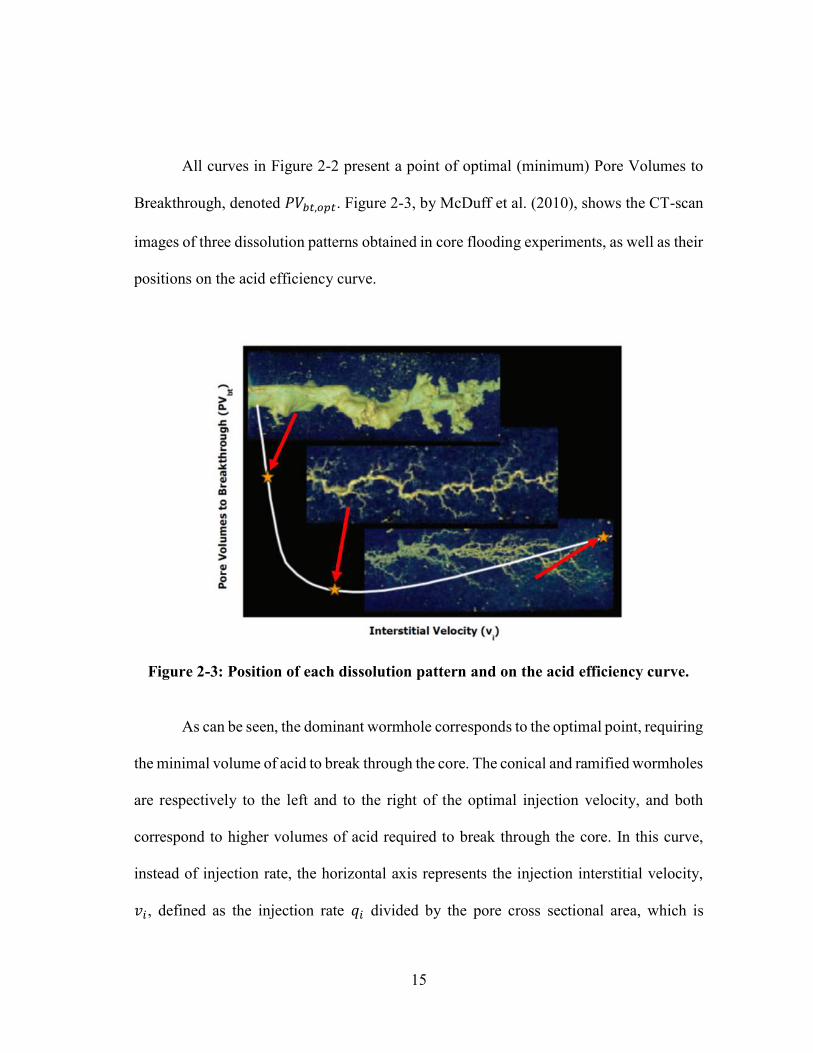
All curves in Figure 2-2 present a point of optimal (minimum) Pore Volumes to

Breakthrough, denoted 𝑃𝑉 , . Figure 2-3, by McDuff et al. (2010), shows the CT-scan

images of three dissolution patterns obtained in core flooding experiments, as well as their

positions on the acid efficiency curve.

Figure 2-3: Position of each dissolution pattern and on the acid efficiency curve.

As can be seen, the dominant wormhole corresponds to the optimal point, requiring

the minimal volume of acid to break through the core. The conical and ramified wormholes

are respectively to the left and to the right of the optimal injection velocity, and both

correspond to higher volumes of acid required to break through the core. In this curve,

instead of injection rate, the horizontal axis represents the injection interstitial velocity,

𝑣 , defined as the injection rate 𝑞 divided by the pore cross sectional area, which is

16

calculated as the product of the cross sectional area of rock 𝐴 and the porosity 𝜙. The

interstitial velocity is the average velocity at which the fluid flows inside the pores. It

differs from the superficial or Darcy velocity, 𝑣, which is just the injection rate divided by

the rock cross sectional area. The interstitial velocity that corresponds to the optimal point

is called optimal interstitial velocity, denoted by 𝑣 , .

The parameters that define the optimal point in the acid efficiency curve, 𝑃𝑉 ,

and 𝑣 , , are of great importance in the design of matrix acidizing operations, as they

relate closely to the ideal flow rate at which the acid should be injected, and how far the

wormholes can penetrate for a given volume of acid.

2.2.1. Models to Find the Optimal Matrix Acidizing Condition

Usually, the optimal conditions for matrix acidizing are obtained by destructive

laboratory core flooding experiments. It is an expensive and time-consuming method, as

each point of the curve requires a whole destructive core flooding experiment.

Several researchers have worked on modeling wormhole formation in carbonate

acidizing, in order to better understand the process, as well as estimate the conditions to

obtain the best results. The first model was probably the one by Schechter and Gidley

(1969), who presented a model based on the pore size distribution and its evolution due to

the surface reaction. Later, Daccord et al. (1987) presented another model based on the

fractal nature of the wormholing phenomenon, devising a quantitative way to relate the

optimal conditions for acidizing.

17

Fredd et al. (1997) and Fredd and Fogler (1999) showed that the different

dissolution patterns correspond to specific ranges of Damköhler number, and the optimal

injection velocity corresponds to a Damköhler number of approximately 0.29, for all rocks

and acids or even chelating agents investigated by them. The Damköhler number is

defined as the ratio of net reaction rate and the rate of acid transport by convection. The

dissolution can be dominated by the reaction rate (in slow reaction systems, such as

limestones with weak acids or dolomites with most acids at low temperatures), or by the

diffusion of the acid or the reaction products.

The existence of the optimal Damköhler number clarifies the competition between

the dissolution rate (including the reaction and diffusion steps) and convection rate of acid.

At small injection velocities (large Damköhler number), the acid has time to react before

being transported by convection, and face dissolution occurs. At too high injection

velocities (small Damköhler number), the acid is transported by convection before it has

time to diffuse to the mineral surface and react, hence forming very ramified wormholes

or uniform dissolution. At the optimal Damköhler number, the convection, diffusion and

reaction rates are perfectly balanced, and only a thin wormhole is formed as the acid is

transported by convection further into the rock.

Theoretically, the existence of the optimal Damköhler number is an interesting

finding, but it is difficult to apply in the field design of acidizing operations, as its

calculation involves many uncertain parameters (pore dimensions and mass transfer

coefficients), and is difficult to upscale from laboratory to the field scale.

18

Other researchers developed models to find the optimal parameters 𝑃𝑉 , and

𝑣 , . Huang et al. (2000a, 2000b) presented another form of the Damköhler number.

Mahmoud et al. (2011) presented a model based on the Péclet number. Dong et al. (2017)

presented a new model based on the statistical analysis of pore size distribution.

Fredd and Miller (2000) and Akanni and Nasr-El-Din (2015) presented

comprehensive reviews of wormhole models. The latter classified these models in seven

categories: capillary tube approach, Damköhler number approach, transition pore theory,

network models, Péclet number approach, semi-empirical approach, and averaged

continuum (or two-scale) models.

The two-scale (or averaged) continuum models are a group of models that

represent the porous medium as a continuum and solve the acid flow using Darcy-

Brinkman-Stokes equation as well as the acid transport and reaction equations, and keep

track of the porous medium dissolution. As the acid dissolves the rock, the porosity

increases, and the model updates the rock permeability, pore radius, and specific surface

area according to the increase in porosity. This model has been implemented by several

researchers (Liu and Ortoleva, 1996, Golfier et al., 2001, Panga et al., 2005, Kalia and

Balakotaiah, 2007, Maheshwari et al., 2012, de Oliveira et al., 2012, Soulaine and

Tchelepi, 2016, Maheshwari et al., 2016, Palharini Schwalbert et al., 2018a).

Some of these researchers (de Oliveira et al., 2012, Maheshwari et al., 2016, and

Palharini Schwalbert et al., 2018a) worked on calibrating the model to match experimental

acid efficiency curves, with satisfactory success. The work published in Palharini

Schwalbert et al. (2019a) is part of this study, presented in section 3.1. However, the model

19

includes internal correlations with adjustable parameters that cannot be measured

experimentally, hence being only useful to represent real data after being calibrated by

history matching experimental data.

There have also been experimental studies focused on finding the optimal

condition with non-destructive measurements (without having to dissolve cores). Tansey

(2015) used CT-scan images of cores to create pore-network models in small scale to

simulate acid injection. He was able to see wormhole formation in the modeling, but not

to predict accurately the optimal conditions. Zakaria et al. (2015) used tracer tests and

related wormhole formation to flowing fraction. The method is promising, but there are

not many results of that yet.

Al-Duailej et al. (2013), Mahmoud et al. (2016), and Mahmoud (2017) used

Nuclear Magnetic Resonance (NMR) to characterize the interconnectivity in the pore

structure and in wormholes and correlate it to the optimum flow rate. It is an interesting

method, but the best results require analyzing the wormholed structure through NMR, so

it is a destructive measurement.

A lot of research and development has been made, but to date the most reliable

values for 𝑃𝑉 , and 𝑣 , are still obtained experimentally by building acid efficiency

curves through core flooding experiments, or by history matching field data of matrix

acidizing jobs.

In fact, even the experimentally obtained curves must be used with caution,

because it has been shown that the parameters 𝑃𝑉 , and 𝑣 , depend strongly on the

dimensions of the cores used in the experiments. This shows the upscaling of the

20

laboratory experimental data to field conditions should be done cautiously, as in the field

treatments the cross sectional areas are several orders of magnitude larger than the cores

used in the experiments. It could be argued that the most reliable data would come from

history matching field data of matrix acidizing jobs.

2.2.1.1. Impact of the Core Dimensions

The impact of the core dimensions is an important but often neglected feature of

wormholing experiments: the measured values of 𝑃𝑉 , and 𝑣 , are very dependent

on the size of the cores used to measure them.

It has been consistently shown that both 𝑃𝑉 , and 𝑣 , decrease as the

diameter of the cores increases (Buijse 2000, Furui et al. 2010, Dong et al. 2014). Figure

2-4 shows plots with the experimental results using different core sizes by Buijse (2000),

Furui et al. (2010), and Dong et al. (2014). In each set of data, everything is the same

except for the core diameter (same acid, mineralogy, core length, similar porosity and

permeability, etc). Different acid-rock combinations were used: Buijse (2000) used 5%

HCl and limestone cores, Furui et al. (2010) used 28% HCl and high porosity chalk, and

Dong et al. (2014) used 15% HCl and Indiana limestone. Figure 2-4 shows the consistent

trend of the core dimension effect in these cases.

21

Figure 2-4: Collection of published data of 𝑷𝑽𝒃𝒕,𝒐𝒑𝒕 and 𝒗𝒊,𝒐𝒑𝒕 comparing different

core sizes. Cohen et al. (2008) and Kalia and Balakotaiah (2009) presented numerical

simulations that agree with these observations. Both Cohen et al. (2008) and Kalia and

Balakotaiah (2009) showed that in numerical simulations of wormholing in linear flow

with domains of different sizes, the wormhole density decreases as the cross sectional area

is increased, leading to a smaller value of 𝑃𝑉 , for larger values of cross sectional area.

While usual values of 𝑃𝑉 , in linear core flooding experiments with small cores

is on the order of 0.5 to 1, other published experiments in large scale also show

consistently small values of 𝑃𝑉 . Walle and Papamichos (2015) studied radial wormhole

propagation in hollow cylinders of chalk, with reported values of 𝑃𝑉 smaller than 0.03.

22

McDuff et al. (2010) studied radial propagation of wormholes in large blocks of

approximately 14 ft3. The values of 𝑃𝑉 can be calculated from the reported injected

volumes of acid at breakthrough, and 𝑃𝑉 lies in the range of 0.03 to 0.14. Izgec et al.

(2009) studied wormhole propagation in vuggy calcite in 4x20 inches cores, reporting

values on the order of 0.1, with some values as low as 0.04.

Furui et al. (2010) presented field data from matrix acidizing operations in more

than 400 wells, both in Middle East limestone and North Sea chalk reservoirs. The median

post-acidizing skin factor of the wells is between -3.5 and -4, corresponding to wormhole

penetrations of 10 to 20 ft, and a 𝑃𝑉 on the order of 0.05. The value of 𝑃𝑉 , measured

in core flooding experiments in this case is on the order of 0.4 (using 1x6 inches cores) to

0.132 (using 4x20 inches cores). Burton et al. (2018) increased the dataset by Furui et al.

(2010), presenting the field results of 654 matrix acidizing treatments from multiple

industry and literature references. Again the median post-acidizing skin factor is between

-3.5 and -4, which corresponds to wormhole penetrations between 10 and 20 ft, and a 𝑃𝑉

on the order of 0.05.

Figure 2-5 (published by Burton et al., 2018) shows the values of 𝑃𝑉 obtained in

experiments with different sample sizes and flow geometries: linear flow in 1 x 6 inch and

4 x 20 inch cores, radial / spherical flow in small blocks 10x10x14 in., large blocks 27.25

x 27.25 x 32 in, and field results. Figure 2-5 shows that 𝑃𝑉 decreases as the rock sample

size increases, until it levels out between the size of the small and large blocks, which are

close to the median field result.

23

Figure 2-5: Comparison of pore volumes to breakthrough (𝑷𝑽𝒃𝒕) for different laboratory scales and field treatments.

2.2.2. Global Models of Wormhole Propagation

Although there are several theoretical approaches to model wormhole propagation,

they are not easily upscaled to field conditions. For this reason, the so-called global models

are usually used for treatment design in the field scale. These are macroscopic semi-

empirical models that “predict the propagation rate of the region around the wellbore

through which wormholes have penetrated” (Economides et al., 2013).

As the wormholes are considered infinitely conductive when compared to the

original reservoir, the wormholed region is regarded as presenting no pressure drop

(Daccord et al., 1987). Hence the estimation of the impact of the matrix acidizing treatment

in the well performance requires only the prediction of the wormholed region.

24

As reviewed by Economides et al. (2013), three are the most commonly used

global models: the volumetric model by Economides et al. (1994), the model from Buijse

and Glasbergen (2005), and the model by Furui et al. (2010). Other available global

models are the ones proposed by Daccord and Lenormand (1987) and Daccord et al.

(1989), Gong and El-Rabaa (1999), Tardy et al. (2007), and Talbot and Gdanski (2008).

The volumetric model was proposed by Hill and published in Economides et al.,

1994. It is a very simple and useful model that assumes a constant value of 𝑃𝑉 . It is an

insightful model that allows a simple prediction of the wormhole length using a single

parameter, 𝑃𝑉 . As it assumes a constant 𝑃𝑉 , it is accurate when the interstitial velocity

is approximately constant during the stimulation time, or if an average value of 𝑃𝑉 is

used. As the flow from a wellbore is usually radial in the near-wellbore region, the

interstitial velocity decreases as the acid reaches longer distances away from the wellbore,

and then the value of 𝑃𝑉 is expected to change with injection time, which is not

accounted for in the volumetric model.

In experiments of radial propagation of wormholes, Daccord and Lenormand

(1987) and Daccord et al. (1989) showed that the wormholes constitute a fractal structure

with fractal dimension 𝑑 ≈ 1.6. They showed the radius of the wormholed region, 𝑟 ,

increases with time following a proportionality such as 𝑟 ∝ 𝑡 , where 𝛼 ≈ 0.65 for 3D

radial structures, and 𝛼 ≈ 0.7 for 2D (thin) radial structures. This translates an important

information regarding wormhole propagation: in these experiments, the value of 𝑃𝑉

decreased as the wormholes propagated away from the center. If 𝑃𝑉 was constant, the

wormholed volume would be linearly proportional to the injected acid volume. In this

25

case, 𝑟 would increase proportionally to the square root of time, hence 𝛼 would be equal

to 0.5. In reality, 𝛼 ≈ 0.65, which means that the wormhole propagation becomes more

efficient as the wormholes propagate. In other words, the effective 𝑃𝑉 decreases as 𝑟

increases.

According to this observation, Daccord and Lenormand (1987) developed a model

of radial propagation of wormholes in which the wormholes grow according to the fractal

dimension (𝑑 ≈ 1.6). A problem of this model is that, although it may be good for

interstitial velocities above the optimal condition, it fails for small, suboptimal velocities.

It does not consider the inefficient suboptimal wormhole propagation. In fact, it does not

predict an optimal condition, and predicts that 𝑟 → ∞ as 𝑞 → 0.

The model by Gong and El-Rabaa (1999) for radial wormhole propagation also

takes into account the fractal dimension presented by Daccord and Lenormand (1987), but

through a combination of dimensionless numbers it captures the existence of the optimal

condition and the inefficient wormhole propagation at smaller flow rate. It shows to be a

promising model, and indeed it was successfully used by McDuff et al. (2010) to match

data obtained from experiments with big blocks of carbonates, which are the largest

wormholing experiments published so far. However, there is a dimensional inconsistency

in this model: the length calculated does not have length dimensions, but rather a

dimension of a length unit to a power of (2/𝑑 ). This would only be a length dimension

if 𝑑 = 2, which is not the case for wormhole propagation (𝑑 ≈ 1.6). This is a theoretical

inconsistency, and in practice it also leads to confusing calculations. For example, if one

26

calculates the injection time to reach a given wormhole length using this model, the

resulting time is different when different length units are used (e.g. feet or meters).

Buijse and Glasbergen (2005) proposed an empirical correlation that matches the

acid efficiency curve of 𝑃𝑉 versus 𝑣 (Figure 2-2), using as input only the coordinates

of the optimum point, 𝑃𝑉 , and 𝑣 , . It seems an excellent correlation to match

experimental data, and it has been used by several researchers. Buijse and Glasbergen

(2005) also presented a way to use the correlation in the radial geometry, which consists

of calculating the interstitial velocity as an average at the front of the wormholed region.

The only parameters required for this model are the coordinates of the optimal

point in the acid efficiency curve: 𝑃𝑉 , and 𝑣 , . This curve follows the shape

observed in experiments, presenting a small wormholing velocity for sub-optimal or too

high interstitial velocities. The radius of the wormholed region can then be calculated with

by integrating the velocity over time.

Tardy et al. (2007) proposed a new model for self-diverting acids, based on Buijse

and Glasbergen’s model. They also proposed a modification of Buijse and Glasbergen’s

model consisting of multiplying that model’s 𝑃𝑉 by a constant. The method for

upscaling from core scale and linear flow to field scale and radial flow proposed by Tardy

et al. (2007) is the same as proposed by Buijse and Glasbergen (2005): use the same

correlation of 𝑃𝑉 versus 𝑣 , with 𝑣 calculated as the average at the wormhole front.

Talbot and Gdanski (2008) proposed another model based on Buijse and

Glasbergen’s, but taking more variables into account, such as acid concentration,

temperature, and core aspect ratio. They provided a means to convert 𝑃𝑉 , and 𝑣 ,

27

data obtained with a given temperature and acid concentration to another temperature and

acid concentration. They include in their model the core aspect ratio, defined by them as

core length divided by cross sectional area. But they do not recommend any means to deal

with this aspect ratio when upscaling from core scale and linear flow to field scale and

radial flow.

The model by Buijse and Glasbergen (2005) and its modifications use directly the

values of 𝑃𝑉 , and 𝑣 , obtained in core flooding experiments (with cores measuring

from 1 inch to a few inches) for making calculations at the wellbore scale. As mentioned

above, even the measurements in the core scale differ significantly when the core diameter

changes. Hence, it should be expected that values of 𝑃𝑉 , and 𝑣 , representative for

the whole wellbore would differ from those measured with cores.

Furui et al. (2010) proposed a new semi-empirical model, based on the correlation

by Buijse and Glasbergen (2005), but with a novel upscaling procedure to model the

wellbore scale. In this model, the values of 𝑃𝑉 , and 𝑣 , for the field scale are

different from those measured at the core scale, and they are not constant, varying

throughout the acid treatment while wormholes propagate. In addition, they modified the

assumption of calculating the interstitial velocity as the average at the outer area of the

stimulated region. Noticing through experiments and numerical simulations that the flow

rate is concentrated at the tips of the dominant wormholes, they proposed that what drives

the wormhole propagation velocity is not simply the average interstitial velocity �̅� , but

the interstitial velocity at the tip of the wormholes, 𝑣 , , which is much greater than the

average value, especially at the field scale.

28

Furui et al. (2012a) presented equations for 𝑣 , for the radial and spherical

propagation of wormholes. The first is applicable for the acidizing of openhole or densely

perforated wells, where the flow field is radial. The latter is applicable when the acid is

injected from small points far from each other, such as a when a limited entry technique

is used with a very small perforation density, when the flow field that arises from each

perforation is spherical.

This model not only estimates a higher wormholing velocity by associating it with

the tip interstitial velocity, but it also estimates a slower declining rate of that velocity. For

the radial propagation of wormholes, e.g., while Buijse-Glasbergen model estimates that

�̅� declines proportional to 1/𝑟 , Furui et al.’s model estimates that 𝑣 , declines

proportional to 1/ 𝑟 (for 𝛼 = 0) or does not decline at all (for 𝛼 = 1), or yet

something in between.

For the cases where this model has been used (Furui et al., 2012a and 2012b), it

presented a better match to field data than the simple use of Buijse-Glasbergen model with

laboratory measured 𝑃𝑉 , and 𝑣 , . However, it has more adjustable parameters,

which have been reported as being hard to estimate, such as 𝑚 , 𝛼 , and 𝑑 , .

Ultimately, these parameters should also be history matched.

The model by Furui et al. (2010) is a very interesting model, as it takes into account

the outcomes obtained at different scales, and it was successfully used to match field data.

However, it has some disadvantages, such as: (1) it needs some important input parameters

that are hard measure or estimate, such as the diameter of the wormhole cluster and the

number of wormholes, (2) sometimes the predicted field results change when the data used

29

as input come from different core sizes, and (3) when it is used to represent the core scale,

it does not reverse back to the correlation by Buijse and Glasbergen, as it should.

A partial objective of this work is to propose a new semi-empirical global model

of wormhole propagation, addressing the issue of upscaling from core flooding data to the

field scale. The new model is presented in section 3.2 and takes into account the different

wormholing results obtained at different scales, and it can use as input the data obtained

using cores of any size, giving the same results. It can be seen as a revisit of the models

by Buijse and Glasbergen (2005) and Furui et al. (2010), as the development of the new

model used a similar approach and many of the same assumptions.

2.2.3. Performance Estimate for Matrix Acidized Wells

The metric usually used to analyze stimulation operations is the post-treatment

skin factor. In matrix acidizing operations in carbonates, the skin factor depends on the

shape of the wormholed region.

2.2.3.1. Radial / Cylindrical Wormholed Region

If the completion of the well to be acidized is openhole or cased and perforated

with a high perforation density, the acid is expected to follow the radial flow field around

the well. In this case, the stimulated region is cylindrical, such as illustrated in the CT-

scans in Figure 1-1.

30

Hawkins (1956) presented the equation for the skin factor resulting of a cylindrical

region of altered permeability around the well, which can be used to calculate the skin

factor of a cylindrical stimulated region around a well in radial flow. If 𝑘 is the original

reservoir permeability and 𝑘 is the permeability of the wormholed region, Daccord et

al. (1987) and Economides et al. (2013) use Hawkins formula with the assumption that

≪ 1, hence − 1 ≈ −1, to calculate the skin factor resulting from a matrix

acidized carbonate.

The radius of the wormholed region, 𝑟 , is usually estimated by a global model,

such as the volumetric, Buijse-Glasbergen’s, or Furui et al.’s model.

2.2.3.2. Heterogeneous Rocks and Diversion

Most carbonate rocks are heterogeneous and show high permeability contrasts, and

this results in complications during the execution of matrix acidizing treatments (Pereira

et al., 2012). Figure 2-6 (by Retnanto et al., 2015) shows an example of high-contrast

permeability distribution in a carbonate reservoir. The more permeable regions receive

more acid, and hence the wormholes grow longer in these regions, and shorter in the less

permeable zones.

The techniques to deal with this problem and enhance the acid penetration in the

low permeability zones are called fluid placement or diversion techniques (Economides et

al., 2013). Even using fluid placement techniques, the final result is usually a

heterogeneous distribution of wormhole penetration, and this must be taken into account

in the skin factor calculation.

31

Figure 2-6: example of permeability profile in a carbonate reservoir.

There are different models to estimate the acid injection into each zone. Basically

they consist of discretizing the wellbore and adjacent reservoir in different segments, each

one with a different permeability, and calculating the injection of acid into each zone along

the time of acid injection. One example of such model developed specifically for

carbonates was presented by Furui et al. (2012b). Other models include the use of different

diverting agents, such as Hill and Galloway (1984), Doerler and Prouvost (1987), Taha et

al. (1989), Schechter (1992), and Nozaki and Hill (2010).

As calculated by these models, the amount of acid injected into each segment is

different, hence the wormhole length is different as well. Hawkins formula is used to

calculate the skin factor in each segment, and an overall skin factor is calculated. For a

32

vertical well, the overall skin factor is easily derived, and is given by equation (2.5). Furui

et al. (2003) presented an analytical equation to calculate the overall skin factor for a

horizontal well.

𝑠 =∫ 𝑘(𝑧)𝑑𝑧

∫𝑘(𝑧)

ln𝑟𝑟

+ 𝑠(𝑧)𝑑𝑧

− ln𝑟

𝑟

(2.5)

where 𝑟 is the external radius of the drainage region of the well, 𝐿 is the length of the

horizontal well, and 𝑠 is the equivalent overall skin factor.

2.2.3.3. Wormhole Propagation in Anisotropic Rocks

Carbonate reservoirs may be fairly isotropic (characteristic of the “pore-type

reservoirs”, Bagrintseva, 2015), or highly anisotropic (“complex-type reservoir rocks”,

Bagrintseva, 2015). In the complex-type reservoirs, vugs, layering, or natural fractures on

different scales contribute to the permeability anisotropy. In these reservoirs, the

dependence of permeability on the direction often varies one, two, or even three or four

orders of magnitude (Bagrintseva, 2015). Vertical permeability is commonly less than

horizontal permeability (Lucia, 2007), but there are cases where the presence of natural

fractures may cause the vertical permeability to be larger than the horizontal (Widarsono

et al., 2006). In some fields, the vertical permeability must often be set as 100 times

smaller than the horizontal permeability to match predicted and historical performance

33

(Lucia, 2007) - in some cases, vertical permeabilities as much as 5000 times smaller than

the horizontal permeability have been used.

To the author’s knowledge, there is no wormhole model for anisotropic

formations, and no consideration regarding the shape of the stimulated zone to be expected

in such cases. There is actually not much published work on the distribution of wormholes

in anisotropic carbonates. The classical assumption for damage distribution in horizontal

wells in anisotropic formations is an elliptical damage distribution, with the ellipse major

axis aligned with the higher permeability direction, such as presented in Furui et al. (2003).

But that does not tell anything about the wormholes distribution when the formation is

acidized.

Widarsono et al. (2006) presented an extensive statistical study of permeability

anisotropy in various carbonate fields using both core plugs and whole cores, and whereas

in most cases the mode of the ratio of vertical to horizontal permeability was in the range

0-0.3, this cannot be regarded as general, and in several cases that value is in the range

0.6-0.9, and in some cases it is even larger than 1. Sahin et al. (2003) presented

measurements of the anisotropy ratio of 108 samples from an Upper Jurassic carbonate

reservoir from Saudi Arabia, with an arithmetic mean in the 20-25 range, but with a mode

smaller than 10. Lake (1988) mentions that even when anisotropy ratios are

experimentally measured to be no more than 2 to 3, measurements of anisotropy in the

field indicate that horizontal permeability can be several factors of 10 larger than vertical

permeability, due to layering in a scale that is not captured in the laboratory measurements.

34

Pichler et al. (1992) presented a result of a simulation with an elliptical distribution

of wormholes, with the major axis aligned with the maximum permeability. However,

Frick and Economides (1993) and Frick and Economides (1996) analyzed carbonate

matrix stimulation in horizontal wells in anisotropic formations, and assumed that in spite

of the damage distribution being elliptic, the wormholes distribution is still cylindrical

around the well, “because stimulation of carbonates relies more on reaction kinetics than

on fluid flow”. However, this seems an unverified assumption, and they commented that

this was still a subject of research. Tardy (2009) presented a method for predicting acid

placement in carbonate reservoirs (including anisotropic formations) that included solving

for the velocity of the acid around the wellbore using the complex potential theory, and

then estimating the wormhole propagation considering the wormholes travel along the

streamlines. This results in wormholes that propagate longer in the direction of higher

permeability.

Nothing was presented on how these anisotropic stimulated regions affect the well

performance. Does it make a difference if the wormhole network is isotropic

(circular/spherical), or anisotropic (elliptical/ellipsoidal)?

Part of the objectives of this research is to model wormhole propagation in

anisotropic formations and study the skin factor of matrix acidized wells in these

formations.

35

2.2.3.4. Wells Stimulated With Limited Entry Technique

One of the techniques to enhance acid placement in heterogeneous rocks is the

limited entry technique, which consists of injecting the acid through just a few entry points

into the formation. This can be achieved in a cased and cemented well with a very small

perforation density (e.g. Burton et al., 2018), or with a special completion that has only a

few access points to the formation (e.g. Fowler et al., 2014). The idea is that the pressure

drop across the injection points during the stimulation treatment is high compared to the

difference in pressure drop between the different formation layers, so the acid is better

distributed.

When this technique is used for the acidizing treatment, the flow pattern that arises

from each injection point is not cylindrical around the well. Instead, in isotropic

formations, the flow field that arises from each injection point is spherical. Furui et al.

(2012a and 2012b) considered this geometry, as can be seen in Figure 2-7 (modified from

Furui et al., 2012a), and developed a skin factor equation for this case. This equation

assumes the formation is isotropic and the wormhole network is spherical. In this work,

the limited entry treatment in anisotropic formations is also studied, proposing different

equations for the skin factor for the cases where neither Hawkins formula nor the equation

by Furui et al. (2012a) can be used. The calculation of the skin factor in this kind of

geometry in anisotropic formations has not been addressed before in the literature.

36

Figure 2-7: Spherical stimulated regions arising from limited entry technique.

2.3. Acid Fracturing

Also called “Fracture Acidizing” by some authors (Kalfayan, 2007), it consists of

creating a hydraulic fracture by injecting a fluid above the breakdown pressure of the

formation, and then injecting an acid to dissolve part of the walls of the created fracture.

The fracture conductivity is created by the differential (heterogeneous) etching of the walls

by the acid dissolution. This method can only be applied in carbonate reservoirs, due to

the high dissolution rate of carbonate minerals in acids. This operation was briefly

introduced in Section 1.2 and illustrated in Figure 1-2 and Figure 1-3.

37

Estimating the productivity of an acid fractured well requires estimating: (1) the

geometry of the created fracture, (2) the acid transport and reaction with resulting etching

of the fracture walls, (3) the conversion of the etching into conductivity distribution along

the fracture, and (4) the result of the created conductivity on the production flow in the

reservoir.

2.3.1. Acid Fracture Models

Modeling the acid fracturing operation involves modeling the rock mechanics to

obtain the fracture geometry, and the acid transport and reaction phenomena to obtain the

distribution of the dissolved rock.

Modeling the propagation of the fracture has received a lot of attention due to the

popularity of the hydraulic fracturing operation with proppant. There are some two-

dimensional analytical solutions that couple the fracture geometry and fluid flow, such as

the PKN model (first created by Perkins and Kern, 1961, and later modified by Nordgern,

1972) and the KGD model (by Khristianovic and Zheltov, 1955, and Geertsma and de

Klerk, 1969), both of them using Sneddon’s (1946) elasticity solution for the stresses

around a pressurized elliptical crack. Both models assume a plane strain state, but in

different directions: PKN assumes a plane strain in the vertical direction, while KGD

assumes plane strain in the horizontal direction. There is also the radial or penny-shaped

fracture model (Geertsma and de Klerk, 1969), where the fracture contour is assumed to

be a circle.

38

PKN and KGD models assume a constant fracture height, which may be a good

assumption if the formations above and below the fractured zone are subject to much

higher horizontal stress, so that the fracture does not propagate upwards and downwards,

growing only in length. The penny-shaped fracture model assumes a circular fracture, and

may be adequate when there is no stress contrast at all. In general, however, the fracture

is expected to propagate in all directions but there are different stress contrasts in different

reservoir layers, and the 2D models are not accurate in these cases.

For such cases three-dimensional (3D) or pseudo three dimensional (p3D) models

can be used. Examples of pseudo-3D models are Cleary (1980), Meyer (1986), and Liu

and Valko (2015). Examples of fully 3D models were presented by Cleary et al. (1983)

and Morita et al. (1988). Commercial software are available for this end as well. Reviews

about different models can be found in Gidley et al. (1989), Economides and Nolte (2000),

and Economides and Martin (2007).

The modeling of acid transport and reaction inside the fracture has been developed

by different researchers. Williams and Nierode (1972) created a model using the analytical

solution that Terrill (1965) developed for heat transfer in the fluid flow between parallel

porous walls, using the analytical perturbation solution for the velocity field given by

Berman (1953). The model consists of analytical solutions obtained using the perturbation

method, assuming laminar incompressible Newtonian fluid, constant fracture width and

leak-off velocity, steady state, and infinite acid reaction rate at the fracture walls.

Roberts and Guin (1975) modified the earlier model by introducing finite reaction

rate in the boundary condition at the fracture walls. Lo and Dean (1989) assumed again

39

infinite reaction rate, but presented a model for injection of multiple fluids. Settari (1993)

made a transient model. The models aforementioned are all one-dimensional in the sense

that they solved for an acid concentration profile along the fracture length only. Settari et

al. (2001) introduced a two-dimensional model, solving for the concentration along the

fracture length and width directions. Romero et al. (2001) introduced a three-dimensional

acid fracture model, still using the approximate analytical solution for the velocity field.

Mou et al. (2010) created a fully three-dimensional model, where both velocity and

concentration were solved in three dimensions. It consisted of a middle scale model with

constant geometry. Oeth et al. (2014) modified Mou’s model developing a field scale acid

fracture model, which solved the velocity and acid fields in three dimensions for the whole

fracture geometry. However, this model was not coupled with the mechanics of fracture

propagation, requiring a separate fracturing model for simulating the fracture propagation.

There is also commercial software for simulating the acid transport and dissolution of the

rock.

Of particular interest in this study is the model developed in-house in this research

group, which consists of a fully coupled model that calculates the fracture propagation to

obtain the fracture geometry, acid transport and reaction, and heat transfer. It is the model

used in this study, with the modifications presented in section 4.2.1. Although the author

did some contributions to the original model, it was mostly developed by Murtada Al

Jawad. The original model is more detailed in Al Jawad (2018) and Al Jawad et al.

(2018a), and it is briefly presented in this text, in section 4.2.

40

2.3.2. Acid Leakoff from Acid Fractures

The basic step for calculating the fracture geometry is the material balance: a

fraction of the total fluid injected during the fracture operation leaks off into the reservoir

porous medium, and the remaining creates the crack. Therefore, an important component

of fracture modeling is the “leakoff” estimation.

The classic leakoff model for fracturing operations was first introduced by Carter

(1957), relating the leaking fluid velocity 𝑣 to a leakoff coefficient 𝐶 divided by the

square root of time. Carter’s leakoff model has been used since its publication, assuming

a constant leakoff coefficient 𝐶 . Howard and Fast (1957) decomposed the leakoff

coefficient into three separate components (𝐶 , 𝐶 , and 𝐶 ), caused by three separate

mechanisms that could retard the leakoff velocity. The three mechanisms are: (1) wall-

building filter cake due to additives in the fracturing fluid (𝐶 ), (2) pressure drop in the

zone invaded by the fracturing fluid’s filtrate (𝐶 ), and (3) reservoir compressive

resistance (𝐶 ). The wall-building coefficient 𝐶 can be determined experimentally by a

filtration experiment, while 𝐶 and 𝐶 can be calculated if the reservoir and leaking fluid

properties are known. These three coefficients can be combined to result in a total leakoff

coefficient, and the relationship of this total leakoff coefficient with time is the same as in

Carter’s model: the leakoff velocity is given by the leakoff coefficient divided by the

square root of time.

However, these models do not take into account the effect of wormhole formation

due to the acid leakoff. Settari (1993) measured acid leakoff experimentally, and proposed

41

an empirical relationship to calculate it, basically relating the leakoff velocity of the acid,

𝑣 , , to the product of the leakoff velocity of the equivalent inert fluid, 𝑣 , , and an

empirical correction factor, 𝑅 , which is always greater than 1. Settari (1993) presented

an empirical curve for 𝑅 , obtained by measuring in cores the leakoff of both inert fluid

and acid. The observed acid leakoff velocity varied with time. Initially, the same leakoff

velocity as the inert fluid was observed (𝑅 = 1), but after some acid was injected, the

leakoff velocity of acid was more than 7 times greater than the inert fluid leakoff velocity.

Hill et al. (1995) presented a new leakoff model, derived in a way similar to

Howard and Fast (1957), but taking into account the existence of wormholes in the invaded

zone. Based on this assumption, Hill et al. (1995) derived an analytical modified leakoff

coefficient for the invaded zone, 𝐶 , , to replace 𝐶 .

This model still has the general behavior in time as given by Carter’s model

(dependence with the square root of time). It consists of a useful analytical model, but

being derived assuming the wormholes are within the invaded zone, it is limited to cases

where 𝑃𝑉 ≥ 1. Using 𝑃𝑉 = 1 in this model results in 𝐶 , → ∞, meaning that the

invaded zone presents no resistance to the leaking fluid. However, the model does not

have a real solution for 𝑃𝑉 < 1.

In some field cases of acid fracturing, premature fracture closure is observed

during the acid injection. This means that while pumping the acid at the designed injection

rate, the pressure falls below the fracture closure pressure. Hence, while pumping the acid,

the fracture is not open anymore. One such example can be seen in Figure 2-8 (by Furui

42

et al., 2012b), where the green line which represents the bottomhole pressure falls below

the fracture closure pressure a few minutes after the acid reaches the reservoir.

Figure 2-8: example of acid fracturing treatment presenting premature fracture closure while pumping the acid.

The presented leakoff models do not predict the premature fracture closure seen in

Figure 2-8, and one of the possible explanations is that those models neglect or

underestimate the existence of long wormholes growing from the fracture face. In fact, the

example presented in Figure 2-8 happened in a field where very efficient wormholing is

expected to happen, as Furui et al. (2012a) estimate an average 𝑃𝑉 for this field to be

around 0.047.

Part of the objectives of this research is to enhance the acid leakoff prediction,

proposing a theoretical leakoff model that can be applied for acid fracturing in cases of

43

efficient wormholing. Such a theoretical model has not been presented yet in the literature,

although there are several reported cases of high leakoff caused by wormhole propagation

(Crowe et al., 1989, Mukherjee and Cudney, 1993, Settari, 1993, Furui et al., 2010,

Aldhayee et al., 2018). The development of the new leakoff model is presented in section

4.1.

2.3.3. Acid Fracture Conductivity

An important step for calculating productivity or injectivity of an acid fractured

well is converting the fracture face dissolution (“etching”) to a conductivity. There are

different correlations available in the literature for that purpose. Fracture conductivity is

defined as the product of fracture width, 𝑤, and fracture permeability, 𝑘 .

Nierode and Kruk (1973) developed the first empirical conductivity correlation

based on laboratory experiments. They related the fracture conductivity to the amount of

dissolved rock, the rock embedment strength (𝑆 ), and the effective confining stress that

pushes the fracture surfaces together, 𝜎 .

Gangi (1978) developed another conductivity correlation based on theoretical

considerations, relating the cubic root of fracture conductivity to the closure stress and

fracture surface asperities. Walsh (1981) presented a model where the cubic root of

fracture conductivity declines logarithmically with the closure stress. Gong et al. (1999)

presented another theoretical correlation accounting for both the rock mechanical

properties and surface roughness. Nasr-El-Din et al. (2008) reevaluated the experimental

44

data by Nierode and Kruk (1973), and recommend using different equations for the

conductivity of acid fractures in limestones and dolomites. Pournik et al. (2009) updated

Nierode and Kruk’s correlation using more experimental results. Neumann (2011)

measured experimentally the conductivity of acid fractures with deep microbial

carbonates, and proposed a correlation similar to Nierode and Kruk (1973), with

dependence only on rock embedment strength, 𝑆 , and effective confining stress, 𝜎 .

More recently, Deng et al. (2012) developed a correlation similar in form to

Nierode and Kruk’s, but where the coefficients are calculated accounting for the rock’s

heterogeneity in both mineralogy and permeability with geostatistical parameters.

Although different in form and origin (empirical / theoretical), all of these

conductivity models assume that the fracture conductivity 𝑘 𝑤 is somehow proportional

to the etched width 𝑤 , and that it decreases when confining stress is increased. They can

be written in the general form:

𝑘 𝑤 = 𝐴𝑤 (2.6)

where the coefficients 𝐴 and 𝐵 are constant for a given rock and confining stress. The

coefficient 𝐴 decreases when the confining stress increases, and the 𝐵 is a constant for a

given model. This general relation is used in this study, in sections 4 and 5, and the

equations to calculate 𝐴 and 𝐵 for different acid fracture conductivity correlations are

presented in Appendix I.

45

2.3.4. Acid Fractured Well Performance

There is an extensive research regarding productivity of propped fractured wells,

but not so many studies on the acid fractured well performance. Economides et al. (2013)

presents a comprehensive review of productivity calculation in propped fractured wells.

Perhaps the most important results for the propped fractured wells are the publications by

Prats (1961), Cinco-Ley and Samaniego (1981), Economides et al. (2002), and Meyer and

Jacot (2005).

Prats (1961) presented a correlation between the fracture conductivity, reservoir

permeability, and an effective wellbore radius that can be converted into a skin factor.

Cinco-Ley and Samaniego (1981) presented a direct relation between the skin factor

resulting from a fracture and the fracture dimensionless conductivity, 𝐶 , defined as the

ratio between the fracture conductivity 𝑘 𝑤 and the product of reservoir permeability 𝑘

and fracture half-length 𝑥 (length of one of the fracture’s wings).

Cinco-Ley and Samaniego (1981) presented the existence of an optimal value for

𝐶 , for a given volume of proppant and a given reservoir. The optimal value, 𝐶 , , is

a function of the reservoir volume and shape and volume of proppant, but for many

conventional cases it is close to 1.6. This means that for a given amount of proppant, there

is an optimal relation between the fracture width and length, and that should be the target

in the fracture design, if possible within physical constraints.

Economides et al. (2002) expanded that analysis to include a broader range of

reservoir scenarios and presented correlations that can be used to calculate the optimal 𝐶

46

and the dimensionless productivity index, based on the reservoir and proppant properties.

This approach for designing a propped fracture is called Unified Fracture Design

(Economides et al., 2002).

Meyer and Jacot (2005) proposed a complex analytical model to calculate the

dimensionless productivity index of fractured wells in closed drainage areas, in pseudo-

steady state. Their model is used for analytical derivations in section 4.5, and it is

presented in more detail in that section.

Ravikumar et al. (2015) presented an optimization procedure for acid fracturing

using the correlations from Unified Fracture Design (Economides et al., 2002). However,

they did not consider in their calculations the uneven conductivity distribution observed

in acid fracturing, nor the operational conditions that allow obtaining, in real acid

fracturing treatments, the 𝐶 , calculated with the correlations. The correlations by

Economides et al. (2002) assume propped fractures to have uniform conductivity along

its length. Acid fractures tend to have a greater conductivity closer to the wellbore and a

small conductivity towards the tip of the fracture. In fact, it is not uncommon to have large

fractions of the created fracture not even contacted by acid, therefore with a very small

conductivity. For this reason, the extension of well performance calculations used for

propped fractures to acid fractures must be tested and better studied.

There are some publications that propose ways to calculate a representative acid

fracture conductivity from the non-homogeneous conductivity distribution, and then use

the same productivity calculations known for the uniform conductivity case. Bennett

(1982) proposed using a simple average of the conductivity along the fracture, while Ben-

47

Naceur and Economides (1989) propose a harmonic average. Raymond and Binder (1967)

presented an alternative way, which considers radial flow in series to add the pressure drop

resulting from each section of the fracture. However, when tested, none of these methods

is accurate for a large range of scenarios.

Some authors used a reservoir simulator to evaluate the fracture productivity by

including the fracture in the reservoir model, as thin grid blocks with heterogeneous

conductivity (Ben-Naceur and Economides, 1989, and Al Jawad et al., 2016). This is an

accurate method, but the need to use two separate simulators, one for acid fracturing and

another one for the reservoir simulation, raises difficulties for optimizing the fracturing

treatment.

Up to date there is no concise method to estimate acid fracture productivity and to

optimize the acid fracturing treatment. To the author’s knowledge there is also no study

that included the existence of the wormholes that grow from fractures faces in the

productivity calculation. Both these topics are addressed in this work, in section 4.3.

2.4. Stimulation Method Selection

The selection of the best stimulation method for a given scenario involves several

considerations, such as the reservoir properties, completion and equipment limits,

operational and environmental aspects, risk assessment, etc. In general, observing all

48

feasibility constraints, the best method is the one that gives the greatest economical return

on investment.

Thomas and Morgenthaler (2000) present a discussion on the selection of

candidate wells for stimulation treatments and the selection of the stimulation technique.

The method they present, which is illustrated in the decision tree in Figure 2-9, involves

basically evaluating all three methods (matrix acidizing, acid fracturing, and propped

fracturing) and selecting the best economical return.

Figure 2-9: decision tree for stimulation method selection.

49

As mentioned in the Introduction, there are studies regarding selection of the

hydraulic fracturing method for a given scenario. That means selecting between acid

versus propped fracturing. Examples of such studies are Ben-Naceur and Economides

(1988), Abass et al. (2006), Vos et al. (2007), Azevedo et al. (2010), Neumann et al.

(2012), Oliveira et al. (2014), Jeon et al. (2016), Suleimenova et al. (2016), and Cash et

al. (2016).

In general, the analysis takes into account that operationally the execution of an

acid fracturing treatment is easier than the execution of a propped fracture (Economides

and Nolte, 2000), but the conductivity of an acid fracture is usually smaller than that of a

propped fracture, especially in high confining stress. In fact, Daneshy et al. (1998) mention

that proppant is usually required in wells with closure stress greater than 5,000 psi.

However, Neumann et al. (2012) discuss the fact that the limit of 5,000 psi is just a general

guideline based on the behavior of shallow soft carbonates, while deeper carbonates may

be mechanically more competent in some cases. Neumann et al. (2012) and Oliveira et al.

(2014) present some results that may expand the limit of 5,000 psi to higher values.

In cases where operational problems lead to costly consequences, such as deep-

water offshore wells, the methods that offer less risk are usually preferred. If matrix

acidizing or acid fracturing can give results similar to the propped hydraulic fracturing,

the first two methods are usually preferred for practical operational reasons.

However, there has not been much study regarding the selection of the stimulation

method between matrix acidizing and acid fracturing. The latter is usually used in less

permeable formations. Daneshy et al. (1998) mention that a general guideline is to use

50

acid fracturing in carbonate reservoirs with permeability smaller than 20md. However,

they do not present a source or a scientific reason for this value. Oliveira et al. (2014)

mention the importance of a criterion to select the best stimulation method between acid

fracturing and matrix acidizing. They mention this criterion is not obvious and does not

yet exist in the literature.

2.5. Research Objectives

The focus of this study is on matrix acidizing and acid fracturing in carbonate

reservoirs. The final objective is to develop a decision criterion to select between these

two methods, the best for a given scenario.

To achieve the final objective, improvements in the current modeling of matrix

acidizing and acid fracturing were done in this study. The partial objectives are:

Improve the global semi-empirical wormhole propagation models for

application to the field scale, accounting for the scaling factor;

Study the productivity of matrix acidized wells in anisotropic reservoirs,

including treatments stimulated with limited entry technique;

Enhance the theoretical prediction of acid leakoff in acid fracturing,

accounting for wormhole propagation in scenarios of efficient wormholing

(𝑃𝑉 ≪ 1);

51

Develop a model to evaluate the productivity of acid fractured wells,

integrated with the in-house fully-coupled acid fracturing model, so that

the integrated model can be used for optimization of acid fracturing

operations;

Develop concise ways to define the best possible result that can be obtained

in a given scenario from both stimulation methods: matrix acidizing and

acid fracturing; hence, define the best method by comparing the maximum

achievable productivity of each.

52

3. IMPROVEMENTS IN MATRIX ACIDIZING MODELING *

In this chapter, the state of the art of modeling matrix acidizing operations is

discussed. Recent improvements developed in this study are presented, including a new

upscaled global model of wormhole propagation and new equations to calculate the skin

factor resultant from matrix acidizing in anisotropic carbonates and / or limited entry

completions. Finally, the design and estimation of the best possible outcome of a matrix

acidizing operation is presented.

3.1. Two-Scale Continuum Model

The two-scale continuum models, also called averaged continuum models, consist

of a group of continuum equations for conservation of mass, chemical species, and

momentum, at the Darcy scale, which are coupled with correlations for evolution of

permeability and other rock properties with porosity as the rock is dissolved. Each element

of the continuum may contain both solid and fluid, and their properties and balance

equations are averaged. These equations are then solved using a numerical method, such

as finite differences or finite volumes methods. Many researchers worked with the

averaged continuum models, using different assumptions and types of fluids or rocks (Liu

* Parts of this section are reprinted with permission from Palharini Schwalbert et al. (2019a), Palharini Schwalbert et al. (2019b), and Palharini Schwalbert et al. (2019c).

53

and Ortoleva, 1996, Golfier et al., 2001, Panga et al., 2005, Kalia and Balakotaiah, 2007,

Maheshwari et al., 2012, de Oliveira et al., 2012, Soulaine and Tchelepi, 2016,

Maheshwari et al., 2016, Palharini Schwalbert et al., 2019a, 2019b, and 2019c).

As it is grounded in the very basic fundamentals of conservation of mass and

momentum, the averaged continuum model can in principle be applied to any kind of rock

and fluid, as long as these are well represented by the properties used in the simulations.

Additionally, any geometry can be simulated, as there is no restricting assumption

regarding the geometry in the model derivation. Isotropic or anisotropic formations can

be simulated as well, without restriction. Many have showed the acceptable comparison

of the model with experimental results (Golfier et al., 2001, Maheshwari et al., 2012, de

Oliveira et al., 2012, Maheshwari et al., 2016 and Akanni, and Nasr-El-Din, 2016),

indicating that it is possible to simulate real data with the averaged continuum model, as

long as tuning is done in the properties and parameters to be used in the simulations to

match the experimental data. However, this model has not been previously used to

simulate wormhole propagation in the field scale, nor to simulate anisotropic rocks. This

application is studied in this work.

Compared with empirical models, averaged continuum models are

computationally expensive to be used even for simulating small cores, and the simulation

of an entire field treatment is computationally unrealistic at present. Additionally, it

requires several inputs that are usually unknown in the field. In this study, this model is

implemented to test its applicability in simulating core flooding experiments and at a

larger scale close to field conditions, as well as to simulate conditions that have not been

54

experimented yet, such as the impact of anisotropic formations and the scale effect in

wormhole propagation.

3.1.1. Mathematical Model

This model was presented in detail by Panga et al. (2005), which is the basis for

the model presented in this work. Some modifications were made, and are mentioned in

the following text. The model is called “two-scale” because it uses some equations at the

Darcy scale, and some correlations at the pore scale. The porous medium is represented

as a continuum in the Darcy scale. The solid and fluid regions are not represented

individually, but it is assumed that at any point, a domain element contains both solid and

fluid in a proportion defined by the porosity at that point. The continuum scale is assumed

to have large enough elements so that each element contains solid and fluid and their

properties can be averaged over the element that englobes that point (the properties are

weighted by the porosity, hence the name “averaged continuum”). Meanwhile the

elements are small enough so that the average properties in each point correctly represent

a relatively homogeneous value within the element, but still the rock heterogeneity is

satisfactorily represented in the variation from one element to the other in the domain.

The formulation presented in this text assumes the fluid phase is composed of a

single aqueous phase. It can be used to simulate acid injection into a water saturated rock,

but not into an oil or gas saturated core. A two-phase version of this model is presented

by Cheng et al. (2019).

55

Each point in space has a given porosity, permeability, velocity, pressure, and acid

concentration. The equations of fluid flow, acid transport, and acid/rock reaction are

solved in a fully coupled way, resulting in the rock dissolution as time progresses. All

properties are heterogeneous, and porosity and permeability evolve with time as the rock

is dissolved.

The single-phase fluid flow is given by the Darcy-Brinkman-Stokes equation,

which is basically the Navier-Stokes equation in terms of superficial velocity, with

Darcy’s Law (𝑼 = −𝜇 𝒌 ⋅ ∇𝑝) added as an additional resistance. Including Darcy’s Law

in the momentum balance equation for a porous medium, with consistent system of units,

the fluid flow is governed by (Soulaine and Tchelepi, 2016):

1

𝜙

𝜕 𝜌 𝑼

𝜕𝑡+ ∇ ⋅

𝜌

𝜙𝑼𝑼 −

𝜇

𝜙∇ 𝑼 = −∇𝑝 + 𝜌 𝒈 − 𝜇𝒌 ⋅ 𝑼

(3.1)

where 𝑼 is the fluid superficial velocity vector (flow rate per rock cross-sectional area,

also called Darcy velocity), 𝜇 is the fluid viscosity, p is pressure, 𝒌 is the rock permeability

tensor, 𝜙 stands for rock porosity, 𝜌 is the fluid density, and 𝒈 is gravity acceleration.

The reason to use Darcy-Brinkman-Stokes equation instead of just Darcy’s law (as

is usual in reservoir simulation) is to be able to represent at the same time the flow in the

porous medium and the free fluid flow, in a single computational domain. This allows the

simulation, for example, of the flow inside an open fracture with the leakoff into the rock,

in a single computational domain, by assigning a porosity of 1 inside the fracture. It is also

56

possible to simulate the fluid flow inside a wellbore, completion, and perforation, and into

the porous medium, at the same time.

In order to solve equation (3.1), the continuity equation is needed to link pressure

and velocity. The continuity equation comes from the mass balance in the fluid phase. In

this case, even considering fluid density as constant, the continuity equation includes a

second term due to the variation of porosity with time:

𝜕 𝜌 𝜙

𝜕𝑡+ ∇ ⋅ 𝜌 𝑼 = 0

(3.2)

The acid chemical species balance is expressed as:

𝜕 𝜙𝜌 𝐶

𝜕𝑡+ ∇ ⋅ 𝜌 𝑼𝐶 − ∇ ⋅ 𝜙𝜌 𝐷 ∇𝐶 = 𝑎 𝜌 𝑅(𝐶 )

(3.3)

where 𝐶 stands for average acid concentration in the fluid at a given location, 𝐷 is

effective diffusivity coefficient of the acid, 𝑎 is mineral specific surface area (unit of area

of fluid-mineral contact per volume of porous medium), the term 𝑅(𝐶 ) is the rate of acid

consumption due to chemical reaction with the rock mineral, and 𝐶 is the acid

concentration at the fluid-solid interface. The acid concentration in this equation is a mass

fraction of acid; for example, 15% acid has 𝐶 equal to 0.15.

Notice that the acid concentration varies within a given pore, being maximum at

the center of the pore and minimum at the fluid-solid contact, where the acid reacts. 𝐶 is

57

the bulk average acid concentration in the fluid phase at a given point that includes a group

of pores. 𝐶 is the acid concentration at the fluid-solid contact, and hence it is 𝐶 that

dictates the reaction rate between acid and mineral. At a given point, 𝐶 is always smaller

than 𝐶 .

In this work the reaction rate is considered to be irreversible and of first order

kinetics, for the sake of simplicity in the acid balance solution. This approach is valid for

the reaction of limestone with fast reacting acids such as hydrochloric acid. This

assumption is used in most literatures of the averaged continuum model, such as Panga et

al. (2005), Kalia and Balakotaiah (2008), Maheshwari et al. (2012), de Oliveira et al.

(2012), and Maheshwari et al. (2016). The first order reaction rate is given by:

𝑅(𝐶 ) = 𝑘 𝐶 (3.4)

where 𝑘 is the surface reaction rate constant, in units of volume of acid consumed per

unit of time per unit of solid-fluid contact surface area per unit of acid concentration. In

units of the International System of Units and with 𝐶 being a mass fraction, 𝑘 has units

of m/s.

The acid molecule that reacts at the fluid-solid contact has to be transported from

the bulk fluid to the solid contact, and the flux of transported acid, 𝐽 , is related to the

mass transfer coefficient 𝑘 and the acid concentrations by:

58

𝐽 = 𝑘 (𝐶 − 𝐶 ) (3.5)

The acid flux that is transported to the fluid-solid contact reacts with the rock

minerals, so equating equations (3.4) and (3.5) results in:

𝑘 𝐶 = 𝑘 (𝐶 − 𝐶 ) (3.6)

Isolating the solid contact acid concentration 𝐶 from Eq. (3.6) it is possible to

obtain the expression of 𝐶 in terms of bulk acid concentration 𝐶 , reaction rate, and mass

transfer coefficients:

𝐶 =𝐶

1 +𝑘𝑘

(3.7)

Substituting Eq. (3.7) into (3.3) we obtain the acid transport equation for a first

order irreversible reaction, which contains only the fluid bulk acid concentration 𝐶 as

unknown. This is the equation to solve for acid concentration in this work:

𝜕 𝜙𝜌 𝐶

𝜕𝑡+ ∇ ⋅ 𝜌 𝑼𝐶 − ∇ ⋅ 𝜙𝜌 𝐷 ∇𝐶 = 𝑎 𝜌

𝑘 𝑘

𝑘 +𝑘𝐶

(3.8)

59

The term is a harmonic mean of reaction rate and mass transfer

coefficients, and can be seen as an effective mass transfer coefficient, as defined in

equation (3.9):

𝑘 =𝑘 𝑘

𝑘 +𝑘

(3.9)

For extremely fast reaction rates, the problem is regarded as mass transfer

dominated, and 𝑘 ≈ 𝑘 . For slow reaction rates, the problem is regarded as reaction

rate dominated, and 𝑘 ≈ 𝑘 .

As the rock dissolution progresses, the porosity field must be updated. The amount

of acid that reacts is directly related to the amount of mineral dissolved through the

gravimetric dissolving power 𝛽 , defined as the mass of mineral dissolved by a unit mass

of pure acid. The porosity evolution is given by equation (3.10), where 𝜌 is the mineral

density.

𝜕𝜙

𝜕𝑡= 𝑎

𝑘 𝑘

𝑘 +𝑘𝐶 𝛽

𝜌

𝜌

(3.10)

The gravimetric dissolving power of the pure acid, denoted by 𝛽 , is defined as

the mass of mineral consumed by a given mass of pure acid (the subscript 100 stands for

100% acid). It is given by stoichiometry as (Economides et al., 2013):

60

𝛽 =𝜐 𝑀𝑊

𝜐 𝑀𝑊 (3.11)

where 𝜐 and 𝜐 are the stoichiometric coefficients of the mineral and the acid in

the dissolution chemical reaction, and 𝑀𝑊 and 𝑀𝑊 are the molecular weights

of the mineral and the acid, respectively. For example, the gravimetric dissolving power

of HCl dissolving calcite is 1.37 kg CaCO3/kg HCl, and for HCl dissolving dolomite it is

1.27 kg MgCa(CO3)2/kg HCl. Pure HCl is never used in field treatments, the usual

concentrations being 15 wt.% or 28 wt.%. The corresponding gravimetric dissolving

powers are given by the product of 𝛽 and the mass fraction of the acid solution. For

example, for 15% HCl, 𝛽 = 0.15𝛽 .

3.1.1.1. Additional Constitutive Relations

The averaged continuum model given by equations (3.1), (3.2), (3.8), and (3.10)

can be solved for velocity, pressure, acid concentration, and porosity, as long as the other

parameters such as 𝐷 , 𝒌, 𝑎 , and 𝑘 are known. Each of these parameters varies with

position and time during the acid injection. For example, the mass transfer coefficient is

known to be affected by local Reynolds number, so it depends on the velocity field. As

the rock is dissolved, its surface area 𝑎 decreases and hence the reaction rate decreases.

Of special interest is the permeability field 𝒌, which is a second order tensor that varies

dramatically as the rock is dissolved and wormholes are formed, and dominates the most

61

important term in the fluid flow equation, Eq. (3.1), which is the Darcy flow contribution

in the Darcy-Brinkmann-Stokes equation.

In order to correctly solve equations (3.1), (3.2), (3.8), and (3.10) for simulating

rock dissolution by an acid system, models for effective diffusivity 𝐷 , rock

permeability 𝒌, and mass transfer coefficient 𝑘 are needed.

The effective diffusion coefficient of the acid species in the porous medium, 𝐷 ,

is different than its molecular diffusivity in a free fluid. In this work, following Soulaine

and Tchelepi (2016) and Nield and Bejan (2006), 𝐷 was calculated using the simple

relation presented in equation (3.12), where 𝐷 is the acid species molecular diffusivity

in the given solvent:

𝐷 = 𝜙𝐷 (3.12)

For the mass transfer coefficient 𝑘 , the most accepted correlations relate

Sherwood number, 𝑆ℎ, to pore scale Reynolds number, 𝑅𝑒 , and Schmidt number, 𝑆𝑐.

The definition of these numbers is presented in equations (3.13), (3.14), and (3.15), and

the correlation used in this work is given in equation (3.16), as used by Panga et al. (2005):

𝑆ℎ =2𝑘 𝑟

𝐷

(3.13)

𝑅𝑒 =2𝑟 𝜌 |𝑼|

𝜇

(3.14)

62

𝑆𝑐 =𝜇

𝜌 𝐷 (3.15)

𝑆ℎ = 𝑆ℎ + 𝑏𝑅𝑒/

𝑆𝑐 / (3.16)

The variable 𝑟 in equations (3.13) and (3.14) stands for the pore radius, which is

also a scalar field that varies with position and time along the calculations. The parameter

𝑆ℎ in Eq. (3.16) is the asymptotic Sherwood number. The value used for it in this work

is 3.66, which is the known value for circular pore throats and is the value used by Panga

et al. (2005), Maheshwari and Balakotaiah (2013), among others. The parameter 𝑏 in Eq.

(3.16) also depends on the pore structure. The value used in this work is 0.7, which is also

the same used by Maheshwari and Balakotaiah (2013).

As the rock is dissolved, porosity increases and the quantities 𝑟 , 𝑎 , and 𝒌 must

be recalculated. The pore radius 𝑟 and the permeability 𝒌 increase, but the specific surface

area 𝑎 decreases, causing the reaction rate to decrease.

A few different correlations have been used for relating 𝑟 , 𝑎 , and 𝒌 to porosity.

Some of them have a theoretical foundation, but with adjustable parameters so that they

can be adjusted to match the expected behavior of a given rock-fluid system. The

correlation used by Maheshwari and Balakotaiah (2013) for permeability evolution, for

example, has two adjustable parameters, 𝛾 and 𝛽, but when both parameters are equal to

1 the correlation reduces to the known Carman-Kozeny equation.

In practice these equations are usually used as empirical data matching, adjusting

the parameters or the equations themselves so that they correctly represent the rock-acid

63

system in study. In the study by Maheshwari and Balakotaiah (2013), for example, despite

the correlation for permeability evolution reducing to Carman-Kozeny equation if 𝛾 = 1

and 𝛽 = 1, the case study presented showed the adjusted values of these parameters to be

𝛾 = 30 and 𝛽 = 9. The equation with these adjusted parameters has no relation with

Carman-Kozeny equation anymore, but it does represent the experimental data in the case

study, so it is a good correlation for that particular rock-acid system.

In this work, the correlations used to relate those pore properties to porosity

evolution are also intended to be used as an empirical tuning, so that the simulations

represent the experimental data. The equations found to best represent the experimental

data in the case study in this work are given in equations (3.17), (3.18), and (3.19), where

𝜙 , 𝑟 , 𝑎 , and 𝒌𝒐 are the initial porosity, pore radius, specific surface area, and

permeability fields, respectively, and 𝛾, 𝜂, and 𝛿 are adjustable parameters. Equations

(3.18) and (3.19) were modified from the ones used by Maheshwari and Balakotaiah

(2013) to have independent power law exponents, to better represent experimental data.

Eq. (3.17) was also modified to be bounded in a realistic region.

𝑟 = 𝑟𝜙

𝜙

(3.17)

𝑎 = 𝑎𝜙

𝜙

1 − 𝜙

1 − 𝜙

(3.18)

𝒌 = 𝒌𝒐

𝜙

𝜙

1 − 𝜙

1 − 𝜙

(3.19)

64

Notice that as 𝜙 → 1, 𝑎 → 0, which makes sense and causes the reaction rate to

be null when 𝜙 = 1 (acid is not consumed if there is no rock to dissolve). For 𝛿 = 1, Eq.

(3.19) reduces to the Carman-Kozeny equation. Also notice that the permeability 𝒌 is a

second order tensor, and so it has different components in an anisotropic field. As the

correction given by Eq. (3.19) for permeability evolution is only scalar, it only changes

the magnitude of the permeability, but the direction remains the same, given by 𝒌𝒐. In

other words, if initially the vertical permeability is 10 times smaller than the horizontal

component, the same ratio between the two components will remain as the porosity

increases and the magnitude of the permeability becomes larger.

3.1.1.2. Numerical Implementation

The averaged continuum model used in this work consists of equations (3.1), (3.2),

(3.8), and (3.10), with the mass transfer coefficient 𝑘 given by equation (3.16), and the

pore radius 𝑟 , specific surface area 𝑎 , and permeability 𝒌 evolution given by equations

(3.17), (3.18), and (3.19). Porosity, mass transfer coefficient, pore radius, specific surface

area are all heterogeneous fields that vary with time, and permeability is a heterogeneous

and anisotropic second order tensor field that also varies with time.

Such a complex group of equations does not have a forthcoming analytical

solution, so a numerical solution is necessary. In this work the numerical solution was

performed through the Finite Volumes Method using the open source Computational Fluid

Dynamics package Open Source Field Operation and Manipulation (OpenFOAM 4.0,

website CFD Direct, 2016).

65

A solver named wormholeFoam was created using the OpenFOAM libraries to

solve the fully coupled transient equations (3.1), (3.2), (3.8), and (3.10). The pressure and

velocity equations were linked using the SIMPLE (Semi-Implicit Method for Pressure

Linked Equations) algorithm. At each time step, after solving the linked pressure and

velocities, Eq. (3.8) is solved for concentration, and then Eq. (3.10) is solved to update the

porosity field due to the dissolved mineral in the current time step. Then equations (3.17),

(3.18), (3.19), and (3.16) are used to update 𝑟 , 𝑎 , 𝒌, and 𝑘 , and the calculation proceeds

to the next time step. Figure 3-1 shows a flowchart diagram illustrating how the equations

are used along the simulation.

Figure 3-1: Flowchart diagram illustrating the simulation sequence.

66

3.1.1.3. Initial Conditions

Before starting the simulation, it is necessary to define the initial porosity,

permeability, pore radius and specific surface area fields. In order to form wormholes, at

least one of these fields should be heterogeneous, in order to cause the instability necessary

to initiate the wormholes.

The actual best heterogeneous fields to represent real rocks consist of a subject that

should be studied more. Not much study has been published relating real geostatistical

distributions for use in the Two-Scale Continuum model to simulate wormhole

propagation. Most of the literature using this model simply uses synthetic distributions of

porosity to generate some instability to originate wormholes in the simulations. Currently,

the most common heterogeneity used in the literature is a random uniformly distributed

porosity field, given by an average value to which is added a uniform random fluctuation

with a certain maximum magnitude. In this work, applications for generating different

types of heterogeneous distributions were created using OpenFOAM. The different

distributions tested in this study are: uniform random porosity distribution given by

equation (3.20), uniform random permeability distribution given by Eq. (3.21), similar

uniform random distributions for 𝑟 and 𝑎 , as well as normal distributions for all four

fields, and lognormal distributions given by Eq. (3.22) for permeability.

𝜙 = 𝜙 1 + 𝑎 (2 ∗ 𝑟 − 1) (3.20)

𝒌 = 𝒌 [1 + 𝑎 (2 ∗ 𝑟 − 1)] (3.21)

67

𝒌 = 𝑒[ ( ) ] 1

𝑘𝒌

(3.22)

In Eq. (3.20) and (3.21), 𝑟 is a uniformly distributed random number between 0

and 1, generated using OpenFOAM's function scalar01(), from the Random library. In Eq.

(3.22), 𝑟 is a standard normally distributed random number, generated using

OpenFOAM's function GaussNormal(). As seed for generating all random numbers the

current computer clock time in seconds was used, so that each time the program is

executed a different random distribution is generated. The parameters 𝑎 and 𝑎 in Eq.

(3.20) and (3.21) are numbers between 0 and 1 that dictate the magnitude of the

heterogeneity. The maximum value of porosity given by Eq. (3.20), for example, would

be 𝜙 = 𝜙 1 + 𝑎 , and the minimum would be 𝜙 = 𝜙 1 − 𝑎 .

In Eq. (3.21) and (3.22), 𝒌 is a tensor that contains the average permeability value

in each direction. For example, if a given rock has mean horizontal permeability 𝑘 and

mean vertical permeability 𝑘 , and x- and z-directions are aligned with the horizontal

permeabilities and y-direction is aligned with the vertical permeability, then the tensor 𝒌 is

given by:

𝒌 =

𝑘 0 0

0 𝑘 0

0 0 𝑘

(3.23)

68

In Eq. (3.22), 𝑘 is the mean permeability value in the direction of maximum

permeability. For example, for the average permeability tensor given in Eq. (3.23), if 𝑘 >

𝑘 , then 𝑘 = 𝑘 . The other parameter in Eq. (3.22), 𝜎 , is the standard deviation of

the natural logarithm of the permeability values. The larger 𝜎 , the larger the heterogeneity

magnitude.

For the case study presented here, the use of a lognormal permeability distribution

as perturbation initiation gave better match between the numerical results and the

experimental data. As mentioned above, this is a topic that should undergo deeper

research, linking state of the art geostatistics to the Two-Scale Continuum model.

3.1.2. Validation of the Model - Experimental Data Matching

In order to validate the model and define parameters, an experimental data tuning

was performed. The experimental data used to tune the model in this work is one of the

experimental curves presented by Furui et al. (2012a): a case of linear acid flooding of a

high porosity chalk with 28%wt. HCl at 150oF in 1-in x 6-in. cores.

The simulations run to match the experimental data were three-dimensional, but

instead of using a cylinder, the numerical domain used to run the simulations is a

parallelepiped with square cross-sectional area having the same cross sectional area of the

1-in diameter core. The use of a square cross sectional area instead of a circular one was

chosen for the sake of simplicity and to assure better numerical stability, as in this case it

is possible to use a structured grid where the grid blocks are also parallelepipeds and have

69

all the same size. An example of the simulation domain used is presented in Figure 3-2.

The grid can be seen in Figure 3-2a, and one example of lognormal permeability field

generated as initial condition can be seen in Figure 3-2b.

(a)

(b)

Figure 3-2: Example of simulation domain for the 1-in x 6-in core. (a) Grid; (b) Lognormal permeability field.

70

Figure 3-3 shows the match between the curve adjusted to experimental points

presented in Furui et al. (2012a) and the results from the simulations performed in this

work. The parameters used in the simulations to match experimental data are shown in

Table 3-1. The values for reaction rate between limestone and HCl and molecular

diffusivity for HCl were obtained in Economides et al. (2013) for the experimental

temperature of 150oF. Porosity and permeability are the values given in Furui et al.

(2012a). Other parameters, such as density and viscosity, are the typical values used for

limestone and straight acid solution. Some parameters, however, such as 𝛾, 𝜂, and 𝛿 for

equations (3.17), (3.18), and (3.19), should be regarded simply as empirical tuning

parameters.

Figure 3-3: Model tuning with experimental data from Furui et al. (2012a).

71

Table 3-1: Parameters and properties used in the numerical simulations

Parameter Description Symbol Units Value

Fluid density 𝜌 kg/m3 1140

Rock mineral density 𝜌 kg/m3 2710

Initial rock mean porosity 𝜙 fraction 0.3

Injected acid concentration 𝐶 mass fraction 0.28

Core diameter - inch 1

Core length - inch 6

Mean horizontal permeability* 𝑘 md 1.5

Mean vertical permeability* 𝑘 md 1.5

Mean initial specific surface area 𝑎 m-1 500

Parameter of lognormal permeability distribution * 𝜎 - 1.1

Mean initial pore radius 𝑟 m 10-5

Dynamic viscosity 𝜇 cP 1.0

Acid molecular diffusivity 𝐷 m2/s 2x10-9

Reaction rate constant 𝑘 m/s 0.015

Acid gravimetric dissolving power 𝛽 - 1.37

Pore radius evolution parameter for Eq. (3.17) 𝛾 - 3

Surface area evolution parameter for Eq. (3.18) 𝜂 - 1

Permeability evolution parameter for Eq. (3.19) 𝛿 - 6

* properties vary in some specific simulations presented in this study, where its variation is indicated

The points of pore volumes to breakthrough in Figure 3-3 correspond to the

expected dissolution patterns. Figure 3-4 shows four examples of the dissolution patterns:

(a) the face dissolution where almost the whole core was dissolved at the injection

interstitial velocity of 0.06cm/min, (b) the conical wormhole at 0.2cm/min, (c) the

dominant wormhole at 2cm/min, and (d) a ramified structure tending to a uniform

dissolution, at 20 cm/min, where there is no clear preferential path but the acid moved

through a large portion of the pores. What is plotted in those figures is the contour of an

72

isosurface with the acid concentration is equal to 14%wt., half of the initial concentration,

at the end of the simulation (breakthrough).

(a) Face dissolution; U=0.06cm/min

(b) Conical wormhole; U=0.2cm/min

(c) Dominant wormhole; U=1.2cm/min

(d) Uniform dissolution; U=20cm/min

Figure 3-4: Dissolution patterns for the points in Figure 3-3. (a) face dissolution, (b) conical wormhole, (c) dominant wormhole, and (d) uniform dissolution.

3.1.2.1. Limitations of the Two-Scale Continuum Model

The match presented in Figure 3-3 is good but not perfect, and some observations

are necessary on the limitations of the two-scale continuum model to represent

experimental data. Some of the parameters, such as 𝛾, 𝜂, and 𝛿, were used simply to match

the data, with no physical meaning and no way of measuring them in the laboratory.

The mean specific surface area, 𝑎 , does have a clear physical meaning and can be

measured in a laboratory. However, the value for 𝑎 that results in the better match

between simulation and experimental data in this study is smaller than what would be

73

measured for a real rock. The specific surface area should be on the order of magnitude of

1 𝑟⁄ or larger. For 𝑟 = 10 𝑚, as in this case, it would be expected to find 𝑎 on the

order of 10 𝑚 or larger. However, the value for 𝑎 that results in the better match in

this study is 𝑎 = 500𝑚 . If a value of 𝑎 = 10 𝑚 was used, it would result in a

much larger optimal injection velocity, as this model predicts that the optimal injection

velocity is somehow proportional to the specific surface area, as presented by Maheshwari

et al. (2012) and also observed in this study.

In this sense, 𝑎 should also be regarded as a tuning parameter, which is certainly

related to the real specific surface area, but is smaller for some reason. A possible

explanation is that at the wormholing regime the acid moves mostly through the larger

pores, which have smaller specific surface area. Hence the effective specific surface area

“observed” in the simulation is smaller than the actual mean specific surface area that

would be measured if all pores were taken into account.

Another observation is that the required refinement of the mesh used in the

simulations depends on the injection velocity: the smaller the velocity, the more refined

the mesh must be. Especially refined meshes are needed to represent the face dissolution

pattern. This can be seen as a limitation of the model or as a consequence of the physics:

the thinner dissolution front resulting from low flow rates require finer meshes to be

simulated. This observation was pointed out by Maheshwari et al. (2012) and Maheshwari

and Balakotaiah (2013), and was also observed in this study. The simulations using

injection velocities equal to or larger than the optimum produced good results when

performed in rather coarse grids, with 2x2x3mm grid blocks (therefore 6,400 grid blocks

74

for the 1x6in. cores simulated). However, in order to capture the face dissolution pattern

in sub-optimal injection velocities, more refined meshes were necessary, with 0.5mm grid

blocks (therefore 616,000 grid blocks for the 1x6in. cores), and still the pore volumes to

breakthrough seems underestimated.

The computation time grows rapidly with the number of grid blocks. The number

of grid blocks in this validation was not too large because small cores were simulated.

However, for large problems where the face dissolution pattern is expected, the number

of required grid blocks might render the simulation unfeasible. Fortunately, in most

practical applications, velocities equal to or larger than the optimal are intended, and so in

the rest of this study the injection velocities used are in the range of the optimal or larger,

and the correct representation of the face dissolution pattern is not a concern. Hence the

larger grid blocks (2x2x2mm) can be used, as they give accurate results for velocities at

or above the optimum.

In this study, a simple personal computer was used for the small scale simulations,

with an Intel Core i5-5200U CPU with 2.2GHz, 8GB RAM. The operating system was

Ubuntu Linux 16.04, and the 3D simulations for spherical propagation of wormholes used

1,000,000 grid blocks, taking about 22 hours to finish in average, and less than 1 hour for

the 2D cases presented. To use this model for field-scale simulations (as presented in

section 3.1.5), for the computation time to be reasonable, parallel computing using a

computer cluster is necessary. That can be done with the present code, as OpenFOAM has

capabilities to parallel running. In order to reduce computation time in field scale

simulations, the mesh used may be coarser far from the wellbore. However, it must be

75

noticed that the wormholes resulting from this model can only be as small as the grid

blocks, hence it is advisable that the grid blocks are refined at least in the region where

wormhole propagation is expected. In the field-scale simulations presented in section

3.1.5, Texas A&M University’s High Performance Research Computing supercomputers

were used, and the larger simulations took more than a month running in 24 cores.

3.1.3. Simulation of 2D Radial Wormhole Propagation

Some simulations were carried out in order to generate a radial distribution of

wormholes, such as the one obtained from an open hole wellbore, where radial flow

develops in the reservoir due to axisymmetry. These radial simulations are two-

dimensional, and a rectangular domain was used, illustrated in Figure 3-5, in order to have

a structured mesh with all grid blocks square and of the same size. All fluid and rock

parameters used are those presented in Table 3-1, the same that resulted in the match

between experimental and numerical data shown in Figure 3-3.

Figure 3-5a shows the whole domain for the radial simulations, which is 0.4 meter

long (x-direction) and 0.8 meter high (y-direction). Figure 3-5b shows a detailed part of

the used mesh. Figure 3-5c shows an example of permeability lognormal distribution for

this mesh, and Figure 3-5d shows a detail of the same permeability field, where the picture

was amplified so the permeability field can be better seen.

76

Figure 3-5: Example of simulation domain for the radial propagation. (a) Whole domain; (b) detail of the mesh; (c) lognormal permeability field; (d) detail of the

lognormal permeability field Figure 3-6 shows the initial acid concentration, where it can be seen that the whole

rock has initially null concentration except for a very small region in the left boundary

where the concentration is equal to the injected acid concentration, in this case 28%wt. or

𝐶 = 0.28. This small region is the acid inlet, and it is shown in detail in Figure 3-6b. The

77

rest of the left boundary is a symmetry plane, so this simulation actually represents only

half of the radial domain, i.e. only 180º of the total 360º.

(a)

(b)

Figure 3-6: Initial condition for acid concentration. (a) Whole domain; (b) detail of

the inlet. As the acid inlet is such a small region compared to the whole rock, a radial flow

is developed, as shown in Figure 3-7, which shows the pressure field for a water injection.

The remaining three boundaries: top, bottom, and right, are outlets maintained at a

constant pressure.

78

Figure 3-7: Example of the radial pressure field that develops with injection.

3.1.3.1. Isotropic rock

Figure 3-8 shows one example of results of the radial wormhole propagation in an

isotropic rock. Figure 3-8a shows the wormholes in a plot of acid concentration. As the

acid goes mostly through the wormholes, the concentration is nearly zero in the rest of the

rock, and the wormholes can be seen clearly in this plot. Figure 3-8b and c show the same

dissolution pattern as Figure 3-8a, but in terms of plots of rock porosity and acid velocity.

While Figure 3-8b shows a lot of ramifications from the main wormholes branches, Figure

3-8c shows that most of the ramifications do not receive acid after a while, so they

propagate only for a short distance, and only the main wormhole branches continue

receiving acid.

79

(a) (b) (c)

Figure 3-8: example of radial propagation of wormholes in isotropic formations.

Plots of (a) acid concentration, (b) porosity, and (c) superficial velocity magnitude. The whole process is stochastic in nature, as it depends on the random initial

properties of the rock. Thus, for the same average porosity, permeability, and other

properties, the wormholes formed in each simulation are different. The number of

wormholes developed also varies from case to case. The most common number, however,

is shown in Figure 3-8, where there are 3 wormholes in the half of the radial domain. As

two of the wormholes are very close to the left symmetry boundary, it could be argued

that the whole radial domain would contain a number between 4 and 6 wormholes.

The number of wormholes in the circular domain is one of the parameters in the

global wormhole model proposed by Furui et al. (2012), which affects how the interstitial

velocity decreases as radial wormholes propagate. From the simulations developed in this

study, the number of wormholes is more likely between 4 and 6 for most rocks, agreeing

with the work of Huang et al. (1999), which indicates that there are approximately 4

80

wormholes at each cross sectional area, and with Furui et al. (2012a), who use 6

wormholes per plane in most of their examples.

Figure 3-9 shows full-domain plots (360º). The acid inlet is at the center of the

domain. Figure 3-9a is a plot of acid concentration, and Figure 3-9b shows acid velocity.

In the velocity plot, it can be seen that 4 main wormhole branches receive most of the acid

and develop further. In the concentration plot, 2 other smaller wormhole branches can be

seen, confirming that the number of wormholes is between 4 and 6. The same patterns

were obtained in the simulations of full or half domains, and because of this the rest of

this section only presents half domain results.

(a) (b)

Figure 3-9: example of radial propagation of wormholes in isotropic formations in the whole 360o domain. Plots of (a) acid concentration, and (b) acid velocity.

Figure 3-10 shows a comparison of a simulation result from this work to a real

experimental CT-scan image of a wormholed rock published by McDuff et al. (2010). The

similarity is remarkable, which supports the conclusion that the simulation results obtained

81

in this work through the averaged continuum model accurately represent the real behavior

of carbonate acidizing, at least qualitatively.

(a)

(b)

Figure 3-10: comparison of (a) simulation result from this work to (b) a real CT-

scan image.

3.1.3.2. Anisotropic Rock

Two different kinds of anisotropy were analyzed in this study: (1) anisotropic

permeability field with different ratios between horizontal and vertical permeability but

the same correlation length so that both permeability components have the same spatial

distribution, and (2) equal values assigned to horizontal and vertical components of

permeability at each grid block, but with different correlation lengths in the horizontal and

vertical directions. In the latter, the scalar permeability values are the same in the

horizontal and vertical directions in each grid block, but it varies in a different length scale

82

in each direction, so that the resulting average horizontal permeability is larger than the

average vertical permeability because of the spatial distribution.

For the first case (𝑘 > 𝑘 , same spatial distribution), the wormholes generate an

elliptical stimulated region, instead of a circular one, with major axis of the ellipse aligned

with the maximum permeability direction (𝑘 in this case). Three different cases of

wormhole anisotropy are shown in Figure 3-11. All cases have the same permeability

anisotropy, with 𝑘 = 10𝑘 , but different injection velocities or permeability

heterogeneity magnitude (𝜎 ). For large injection velocities and small permeability

heterogeneity magnitude, the wormholes tend to be aligned with the maximum

permeability direction, and tend to be longer in that direction. It can be seen that increasing

the injection velocity makes the wormholes more anisotropic (longer in the maximum

permeability direction). In addition, increasing 𝜎 seems to make the wormholes less

anisotropic.

83

(a)

(b)

(c)

(d)

Figure 3-11: simulation results for anisotropic rocks, with 𝒌𝑯 = 𝟏𝟎𝒌𝑽, where

anisotropic wormhole distribution is observed. (a) 𝑼𝒊𝒏𝒍𝒆𝒕 = 𝟏𝟎𝟎𝒄𝒎/𝒎𝒊𝒏, 𝝈𝒌 = 𝟎. 𝟐. (b) 𝑼𝒊𝒏𝒍𝒆𝒕 = 𝟐𝟎𝟎𝒄𝒎/𝒎𝒊𝒏, 𝝈𝒌 = 𝟎. 𝟐. (c) 𝑼𝒊𝒏𝒍𝒆𝒕 = 𝟐𝟎𝟎𝒄𝒎/𝒎𝒊𝒏, 𝝈𝒌 = 𝟎. 𝟒. (d)

Illustration of the elliptical stimulated region. However, for small injection velocities, the wormholes are still formed in a circular

isotropic radial pattern, not following the permeability anisotropy. This is shown in Figure

3-12.

84

(a)

(b)

Figure 3-12: simulation results for anisotropic rocks, with 𝒌𝑯 = 𝟏𝟎𝒌𝑽, where the wormhole distribution does not follow the permeability anisotropy. (a) 𝑼𝒊𝒏𝒍𝒆𝒕 =

𝟐𝟎𝒄𝒎/𝒎𝒊𝒏, 𝝈𝒌 = 𝟏. 𝟐. (b) 𝑼𝒊𝒏𝒍𝒆𝒕 = 𝟒𝟎𝒄𝒎/𝒎𝒊𝒏, 𝝈𝒌 = 𝟎. 𝟖. A possible explanation for this peculiar behavior is that at larger injection

velocities the convection dominates over the reaction, and the acid is forced in the high

permeability direction before it has time to react, and hence the wormholes are directed to

the higher permeability direction; with smaller injection velocities, convection is not that

strong and the acid reacts before being directed to the higher permeability direction, hence

increasing the local permeability and creating more conical wormholes dictated by the

local heterogeneities, but not necessarily aligned with the permeability. In the case of high

injection velocity, wormholes follow the mean maximum permeability direction and an

elliptical stimulated region is created.

The fact that the anisotropic wormhole propagation happens at high injection

velocities may be related to the optimal injection rate. It is expected that for very small

injection rates, where the face dissolution regime occurs, the dissolution should not depend

85

on the flow field. Although the injection velocities shown in Figure 3-12 may seem high,

the area of the injection inlet is very small (0.16 cm2), so that the injection rate is actually

small. The interstitial velocity goes below the optimal after a short while. For example,

for the case in Figure 3-12a, where 𝑈 = 20𝑐𝑚/𝑚𝑖𝑛, the interstitial velocity falls

below the optimal (2 cm/min) when the wormholes reach 5 cm. As the domain measures

80 cm by 40 cm, the interstitial velocity falls below the optimal long before the wormholes

break through.

Based on these results, comparing Figure 3-11 and Figure 3-12, it seems that the

interstitial velocity required for the wormholed region to propagate elliptically is on the

order of the optimal interstitial velocity for wormhole propagation.

The second type of anisotropy investigated in this study is related to the spatial

distribution of permeability. In these cases, each grid block had the same value for the

permeability component in all directions (𝑘 = 𝑘 in each grid block), so the permeability

could have been a scalar quantity. However, the spatial distribution of the permeability

was not the same in both directions. It was more correlated in the horizontal direction,

resulting in an average horizontal permeability for the whole rock greater than the average

vertical permeability.

The permeability correlation length is a geostatistical parameter representing the

distance from a point beyond which there is no further correlation of the permeability

associated with that point. In these cases, the correlation length in the horizontal direction,

𝜆 , is larger than the correlation length in the vertical direction, 𝜆 . This means that when

the permeability correlation length is greater in the horizontal direction than in the vertical

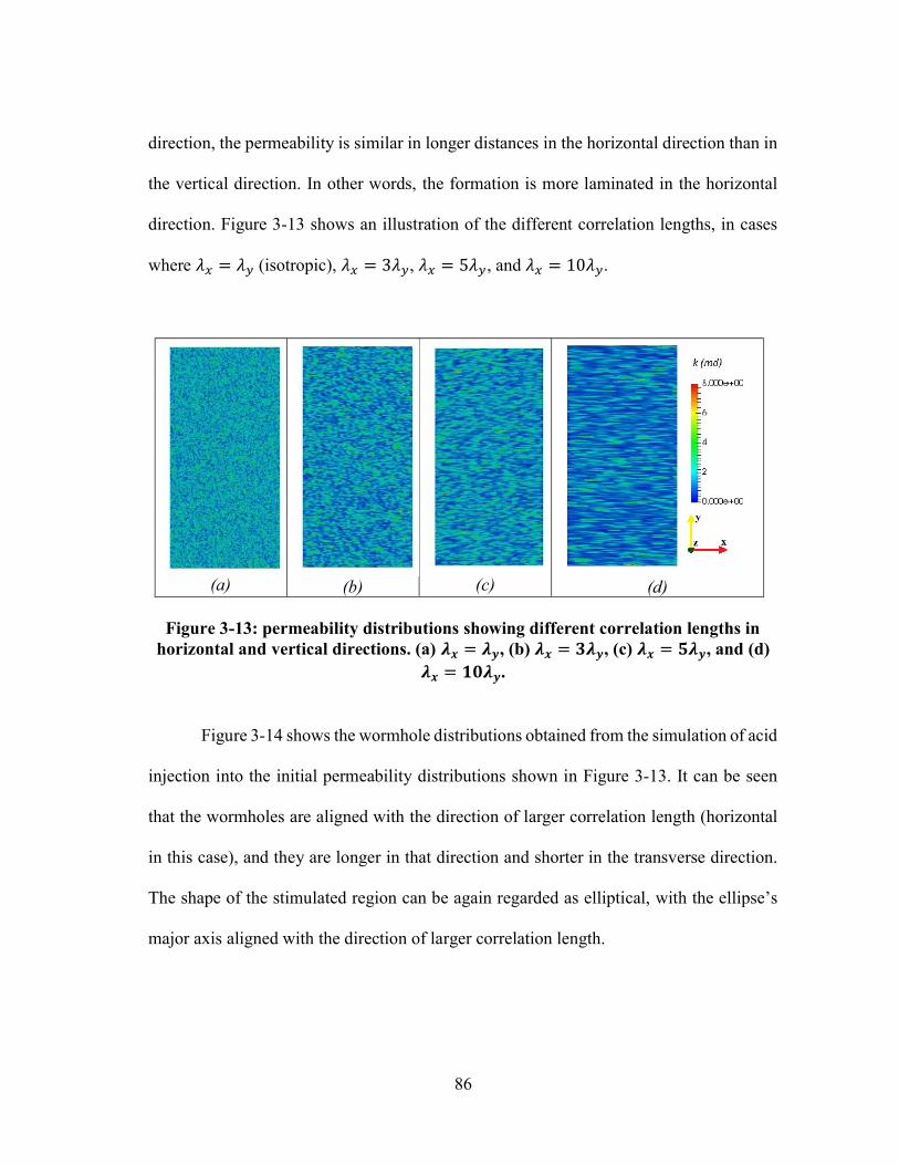
86

direction, the permeability is similar in longer distances in the horizontal direction than in

the vertical direction. In other words, the formation is more laminated in the horizontal

direction. Figure 3-13 shows an illustration of the different correlation lengths, in cases

where 𝜆 = 𝜆 (isotropic), 𝜆 = 3𝜆 , 𝜆 = 5𝜆 , and 𝜆 = 10𝜆 .

(a) (b)

(c)

(d)

Figure 3-13: permeability distributions showing different correlation lengths in

horizontal and vertical directions. (a) 𝝀𝒙 = 𝝀𝒚, (b) 𝝀𝒙 = 𝟑𝝀𝒚, (c) 𝝀𝒙 = 𝟓𝝀𝒚, and (d) 𝝀𝒙 = 𝟏𝟎𝝀𝒚.

Figure 3-14 shows the wormhole distributions obtained from the simulation of acid

injection into the initial permeability distributions shown in Figure 3-13. It can be seen

that the wormholes are aligned with the direction of larger correlation length (horizontal

in this case), and they are longer in that direction and shorter in the transverse direction.

The shape of the stimulated region can be again regarded as elliptical, with the ellipse’s

major axis aligned with the direction of larger correlation length.

87

(a)

(b)

(c)

(d)

Figure 3-14: wormhole distributions obtained in the simulations with permeability distributions showing different correlation lengths in horizontal and vertical

directions. (a) 𝝀𝒙 = 𝝀𝒚, (b) 𝝀𝒙 = 𝟑𝝀𝒚, (c) 𝝀𝒙 = 𝟓𝝀𝒚, and (d) 𝝀𝒙 = 𝟏𝟎𝝀𝒚. This alignment of the wormholes with the permeability had never been reported

before. However, it can be observed experimentally. Figure 3-15 (provided by Shirley,

2019, obtained as part of the research published in Shirley and Hill, 2019) shows real CT-

scan images of two different wormholed cores aligned with the porosity laminations

(usually related to high permeability). On both Figure 3-15a and b, the picture on the left

shows CT-scans of the original rock, before acid injection, where laminations of high

porosity can be seen clearly. The picture in the middle shows an intermediate state, where

the wormhole had gone about halfway through the core, and the picture on the right is a

CT-scan after the wormhole broke through the cores. In both Figure 3-15a and b, the

wormholes seem to form aligned with the laminations, until the lamination ends and the

wormholes deviate towards the next lamination of high porosity.

88

Figure 3-15: CT scans cores with wormholes aligned with the original rock laminations

The same behavior shown in Figure 3-15, obtained experimentally, is observed

when simulating linear core flooding using virtual cores with initial inclined laminated

porosity. The simulation results for three different cores are shown in Figure 3-16. In all

three cores there are inclined porosity and permeability laminations, as shown in the

pictures labeled “initial porosity”. In all cases, the wormholes propagate along a

lamination. At some point the wormholes reach a wall and are forced into the matrix, until

they find another lamination. The comparison of Figure 3-15 and Figure 3-16 shows

remarkable similarity, illustrating again how the Two-Scale Continuum model represents

real wormholing behavior, as long as the input used is representative of the real rock to be

simulated.

89

Figure 3-16: Simulation of linear core flooding in cores with inclined porosity laminations.

3.1.4. Simulation of Spherical Wormhole Propagation

To simulate flow from a single acid inlet in a treatment performed using limited

entry technique, we ran some cases of spherical distribution of wormholes. As in a limited

entry completion, each acid inlet is far from the others, and spherical flow arises from each

acid entry point, until a distance at which the pressure field from one “senses” the others.

The stimulated region in these cases is expected to be spherical too. The spherical flow is

three dimensional, and a cubic domain as illustrated in Figure 3-17 was used. All fluid and

rock parameters used are those presented in Table 3-1, the same that resulted in the match

between experimental and numerical data shown in Figure 3-3.

90

(a)

(b)

(d)

Figure 3-17: Example of simulation domain for the spherical wormhole

propagation. (a) Whole domain and mesh; (b) detail of the mesh; (c) lognormal permeability field; (d) detail of the acid inlet.

Figure 3-17a shows the whole computational domain used for the spherical flow

simulations, which is a cube with a side of 0.2m. The acid inlet is located at a single corner

of the cube, around x=0, y=0, z=0. Figure 3-17b shows a detail of the mesh. Figure 3-17c

shows an example of permeability lognormal distribution for this mesh. Figure 3-17d

shows the initial acid concentration, where it can be seen that the whole rock has initially

91

null concentration except for the acid inlet, where the concentration is equal to the injected

acid concentration, in this case 28%wt. or 𝐶 = 0.28. The simulation domain is only 1/8

of the total domain because of the symmetry assumption.

3.1.4.1. Isotropic Rock

One of the results for isotropic rocks is shown in Figure 3-18, which presents the

isosurface of 14% acid concentration before the wormhole breakthrough. The process is

stochastic in nature, as it depends on the random initial properties of the rock. Hence, the

number and shape of wormholes developed varies from case to case. The most common

number of wormholes, however, is that shown in Figure 3-18, where there are 3

wormholes in the simulation domain, which is 1 8 of the total spherical domain. As 2 out

of the 3 wormholes are developed very close to the symmetry boundary, it can be

concluded that 1 or 2 of those 3 wormholes is shared with another 1 8 of the whole domain

(such as observed in the radial simulations near the symmetry planes). That would make

a total of 16 to 24 wormholes for the whole spherical domain, which agrees well with the

original assumption of 20 wormholes made by Furui et al. (2012a).

92

(a)

(b)

Figure 3-18: Simulation results of the spherical wormhole propagation for an

isotropic formation. (a) Wormholes only; (b) wormhole network inside the simulation grid.

The presence of the wormholes close to the symmetry boundaries makes it hard to

define what is the effect of the spherical flow and interaction between wormholes and

what is the effect of interaction with the symmetry boundary. To clarify this point, future

simulations should consider simulating the whole spherical domain.

3.1.4.2. Anisotropic Rock

The results obtained for the 3-D simulation of the spherical wormholes distribution

are similar to the 2-D simulations of radial wormhole propagation. In the radial

propagation in anisotropic formations, an elliptic stimulated region was observed if the

injection rate was high enough. In the spherical propagation, an ellipsoidal stimulated

region is developed if the injection rate is high enough. In the simulations performed in

this study the x- and z-directions are regarded as horizontal, and the y-direction is regarded

93

as vertical. The permeability components in both horizontal directions are the same, 𝑘 =

𝑘 = 𝑘 , but the vertical component is different, and in the results shown here it is ten

times smaller (𝑘 = 𝑘 = 0.1𝑘 ). As there are two horizontal directions and only one

vertical direction, the ellipsoidal stimulated region is oblate, i.e., there are two horizontal

major axes and one vertical minor axis.

Just as in the radial case, the simulations show that for higher injection velocities

the wormholes are more strongly aligned with the maximum permeability directions, and

are longer in this direction, as shown in Figure 3-19. Again, the wormholes shown in the

pictures are isosurfaces of half of the injected acid concentration. Although the injection

velocities seem high, it must be remembered that the inlet area is small (0.48 cm2), so that

the injection rates are not so high. In fact, in all three cases shown in Figure 3-19 the

interstitial velocity falls below the optimum before the breakthrough. For the cases in

Figure 3-19a, b, and c, the interstitial velocity falls below the optimum when the

wormholes reach the length of 3.6 cm, 6.2 cm, and 8 cm, respectively.

94

(a)

(b)

(c)

(d)

Figure 3-19: results of the simulation of the ellipsoidal wormhole network

developed from acid injection in an anisotropic carbonate rock. (a) 𝑼𝒊𝒏𝒍𝒆𝒕 =𝟐𝟎𝟎𝒄𝒎/𝒎𝒊𝒏, (b) 𝑼𝒊𝒏𝒍𝒆𝒕 = 𝟔𝟎𝟎𝒄𝒎/𝒎𝒊𝒏, (c) 𝑼𝒊𝒏𝒍𝒆𝒕 = 𝟏𝟎𝟎𝟎𝒄𝒎/𝒎𝒊𝒏, (d) detail of the case (c) inside the simulation domain, showing the difference between vertical

and horizontal wormhole propagation. Simulations were also carried out with different spatial variation of the

permeability, and again the results were analogous to those obtained in the radial

simulations: wormholes grow longer in the directions of higher permeability correlation

length. If both horizontal directions (x- and z-directions) show a longer correlation length

than the vertical direction (y), then the wormholes propagate more in the horizontal

95

directions. Again, the shape of the stimulated region is an oblate ellipsoid, with minor axis

aligned with the direction of smaller correlation length.

The impact of these anisotropic wormhole networks on field treatments is

discussed further in section 3.3.

3.1.5. Large Scale 3D Simulations

Most results presented so far involved small scale simulations. Some larger scale

simulations were also conducted to observe the wormhole propagation in a scale and

geometry closer to real field treatments. The parameters used in these large scale

simulations were slightly different to have better numerical stability and faster

convergence. These parameters are listed in Table 3-2. In this case, the acid concentration

used is 15% HCl.

96

Table 3-2: Parameters and properties used in the large scale numerical simulations

Parameter Description Symbol Units Value

Fluid density 𝜌 kg/m3 1070

Rock mineral density 𝜌 kg/m3 2710

Initial rock mean porosity 𝜙 fraction 0.15

Injected acid concentration 𝐶 mass fraction 0.15

Mean horizontal permeability 𝑘 md 1

Mean vertical permeability 𝑘 md 1

Mean initial specific surface area 𝑎 m-1 500

Parameter of lognormal permeability distribution 𝜎 - 1

Mean initial pore radius 𝑟 m 10-5

Dynamic viscosity 𝜇 cP 1.0

Acid molecular diffusivity 𝐷 m2/s 2x10-9

Reaction rate constant 𝑘 m/s 0.015

Acid gravimetric dissolving power 𝛽 - 1.37

Pore radius evolution parameter (for Eq. (3.17)) 𝛾 - 3

Surface area evolution parameter (for Eq. 3.17) 𝜂 - 1

Permeability evolution parameter (for Eq. 3.18) 𝛿 - 4

Grid block length (cubic grid blocks) m 0.01

Three-dimensional simulations of radial wormhole propagation from a wellbore

with the actual diameter of a real wellbore, 7 in., were conducted. Injection rates of

0.1 𝑏𝑝𝑚/𝑓𝑡 and 0.2 𝑏𝑝𝑚/𝑓𝑡 were simulated, on the order of the injection rates used in

the field. Only a few feet of wellbore length were simulated. Due to computational power,

it was not possible to simulate a whole usual wellbore length. But different wellbore

lengths were simulated to make sure the results stabilized as the wellbore length increases,

so the simulation domain is believed to be representative of a longer length. Figure 3-20

shows one example of the resulting wormhole network (porosity isosurface). The diameter

of the inner wellbore in this figure measures 7 in.

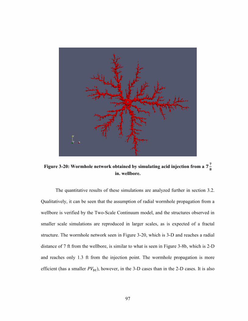
97

Figure 3-20: Wormhole network obtained by simulating acid injection from a 𝟕𝟕

𝟖

in. wellbore. The quantitative results of these simulations are analyzed further in section 3.2.

Qualitatively, it can be seen that the assumption of radial wormhole propagation from a

wellbore is verified by the Two-Scale Continuum model, and the structures observed in

smaller scale simulations are reproduced in larger scales, as is expected of a fractal

structure. The wormhole network seen in Figure 3-20, which is 3-D and reaches a radial

distance of 7 ft from the wellbore, is similar to what is seen in Figure 3-8b, which is 2-D

and reaches only 1.3 ft from the injection point. The wormhole propagation is more

efficient (has a smaller 𝑃𝑉 ), however, in the 3-D cases than in the 2-D cases. It is also

98

more efficient in larger scales than in small scales, which has been observed

experimentally and is discussed further in section 3.2.

Figure 3-21 shows the comparison of a three-dimensional large scale simulation

(7 in. diameter by 3 ft long wellbore) with a real CT-scan image of a wormholed rock.

Figure 3-21a shows the simulation result, while Figure 3-21b was published by McDuff

et al. (2010), consisting of a 14 ft3 block of limestone, the largest scale wormhole

propagation experiment published to date. The resemblance is remarkable, showing again

that the Two-Scale Continuum Model is suitable to reproduce real wormhole structures,

at least qualitatively.

(a) 3D simulation result (b) real CT-scan image

Figure 3-21: comparison of (a) 3D simulation result to (b) a real CT-scan image. Figure 3-20 and Figure 3-21 show the simulation of wormhole propagation from

an openhole wellbore. Simulations were also conducted to investigate how wormholes

propagate from a cased, cemented, and perforated wellbore. Figure 3-22 shows a result of

99

one of these simulations. Figure 3-22a shows the initial wellbore (7 in. diameter by 2 ft

long) with the single perforation tunnel. The wellbore walls are impermeable in the

simulation, so all the acid injection into the rock comes from the perforation. Figure 3-22b

shows the resulting wormhole network that originated from the perforation, and a pressure

contour around it. The diameter of the wellbore in this figure measures 7 in.

Figure 3-22: simulation of wormhole propagation from a cased, cemented, and perforated wellbore. (a) wellbore with perforation; (b) wormhole network with a

pressure contour. The wormholes propagate radially, originating from the perforation. As can be

seen in the pressure contour, the stimulated region is practically cylindrical, regardless of

the acid injection coming from the perforation, and not from the wellbore walls, which are

cased. The cylindrical stimulated region seems to be centered around the perforation, and

not around the wellbore.

100

As mentioned in section 3.1.2.1, in this study, a simple personal computer with an

Intel Core i5-5200U CPU with 2.2GHz and 8GB RAM was used for the small scale

simulations (sections 3.1.2, 3.1.3, and 3.1.4). The 2D cases presented took less than 1 hour

of computation time, while the 3D simulations for spherical propagation of wormholes

used 1,000,000 grid blocks, taking about 22 hours to finish in average. However, for the

field-scale simulations (as presented in section 3.1.5), for the computation time to be

reasonable, parallel computing using a computer cluster is necessary. In the field-scale

simulations presented in this section, Texas A&M University’s High Performance

Research Computing supercomputers were used, and the larger simulations such as shown

in Figure 3-20 took more than a month running in 24 cores.

3.2. New Upscaled Global Model for Wormhole Propagation

Section 3.1 illustrated the implementation and use of the Two-Scale Continuum

model to simulate wormhole propagation. It is a useful model that can correctly represent

real acidizing of carbonate formations, both quantitatively and qualitatively, if tuned to a

given rock / acid system. However, nowadays it is not practical enough to be used as an

engineering tool to design field matrix acidizing treatments. This is because: (1) it is too

time consuming to run and (2) it requires too many input data that are hard to measure,

and some input parameters that do not have physical meaning and cannot even be

measured. Both points are discussed in section 3.1.2.1.

101

For these reasons, the global or semi-empirical models of wormhole propagation

are more useful for field treatment design. Most global models are simple correlations that

can be used in a spreadsheet or even hand calculations, and take as input experimental

data obtained in core flooding experiments (e.g. 𝑃𝑉 , and 𝑣 , ). However, as

discussed in section 2.2.1.1, the diameter of the core has a large impact on the experimental

values of 𝑃𝑉 , and 𝑣 , , showing that the wormhole propagation is not a scale-

independent problem. As discussed in section 2.2.2, most global wormhole models do not

take the scale factor into account satisfactorily.

The objective of this section is to present a new semi-empirical model of wormhole

propagation that gives a prediction of 𝑟 for different scales (core scale and field scale),

and that can be used for different flow geometries (linear, radial, and spherical flow). The

upscaling of the model to field application is considered in the model development. The

model proposed in this study is but a simple modification of the previously published

models by Buijse and Glasbergen (2005) and Furui et al. (2010), presented in section 2.2.2,

and it can be seen as an upscaling procedure from core to field scale.

3.2.1. Corrections for the core diameter

Figure 2-4 shows that different researchers have published that both 𝑃𝑉 , and

𝑣 , decrease as the core diameter increases (Buijse, 2000, Furui et al., 2010, Dong et al,

2014). Based on the data in Figure 2-4, two simple empirical correlations are proposed to

relate 𝑃𝑉 , and 𝑣 , to different scales:

102

𝑃𝑉 , , = 𝑃𝑉 , ,

𝑑

𝑑

(3.24)

𝑣 , , = 𝑣 , ,

𝑑

𝑑

(3.25)

where 𝑃𝑉 , , and 𝑃𝑉 , , are the optimal pore volumes to breakthrough measured

using cores of diameters 𝑑 and 𝑑 , respectively. Analogously, 𝑣 , , and 𝑣 , , are the

optimal interstitial velocities measured using cores of diameters 𝑑 and 𝑑 , respectively.

To obtain the two parameters for scaling, equations (3.24) and (3.25) are used to match

the available experimental data, as shown in Figure 3-23. In this figure, 𝜀 ranges from

0.53 to 0.95, and 𝜀 from 0.63 to 1.34. Notice that the higher value of 𝜀 and 𝜀 from the

small number of data points (the work by Furui et al., 2010, and Buijse, 2000) may not be

as reliable as the smaller values of 𝜀 and 𝜀 from the data set by Dong et al. (2014).

103

Figure 3-23: Match of proposed correlations (3.24) and (3.25) to published data.

3.2.1.1. Reasons for the Variation of 𝑷𝑽𝒃𝒕,𝒐𝒑𝒕 and 𝒗𝒊,𝒐𝒑𝒕 with the Core Size

The main reason of 𝑃𝑉 , and 𝑣 , decreasing as the core diameter increases is

that for the larger cores the wormhole density is smaller, as observed by Buijse (2000),

Cohen et al. (2008), Kalia and Balakotaiah (2008), Furui et al. (2010), and Dong et al.

(2014). With less wormholes per unit volume, the mass of mineral actually dissolved is

smaller, hence a smaller volume of acid is required to dissolve it, resulting in a smaller

𝑃𝑉 , . Also, the existence of less wormholes per unit volume means that a higher flow

rate is concentrated in each wormhole. Thus, the smaller the wormhole density, a smaller

104

overall average interstitial velocity is required to have the same optimal velocity at the tip

of the wormholes, as observed by Furui et al. (2010).

The same behavior is observed in radial flow. As the wormholes propagate away

from the central injection point, the wormhole density per unit volume decreases. This

happens because wormholes propagate according to a fractal geometry. Daccord and

Lenormand (1987) and Daccord et al. (1989) measured the fractal dimension in radial

propagation of wormholes to be around 1.6. If the wormhole density was constant as the

wormholes propagate radially, the volume of the wormholed region would be proportional

to 𝑟 , hence the “fractal” dimension would be 2. The fact that the fractal dimension is

1.6 implies that the wormhole density decreases as 𝑟 increases. This can be seen in the

experimental pictures presented by Daccord and Lenormand (1987) and McDuff et al.

(2010), or the simulation results presented in this study, Figure 3-8, Figure 3-9, Figure

3-20, and Figure 3-21. In all cases, the wormhole density is larger near the center. Because

of the decrease in wormhole density as 𝑟 increases (less wormholes per unit rock

volume), 𝑃𝑉 , decreases.

Because of the flow concentration at the wormhole tips, 𝑣 , is also expected to

decrease as 𝑟 increases. Appendix A presents an analysis of radial propagation of

wormholes, illustrating the concentration of flow velocity at the wormhole tips and the

decrease in wormhole density as 𝑟 increases.

105

3.2.1.2. Limit for the Decrease of 𝑷𝑽𝒃𝒕,𝒐𝒑𝒕 and 𝒗𝒊,𝒐𝒑𝒕

Burton et al. (2018) compared values of 𝑃𝑉 for different scales (see Figure 2-5).

They showed that the value obtained in the large block experiments by McDuff et al.

(2010) matches closely the values of 𝑃𝑉 observed in field treatments. This indicates that

there is some scale large enough for the wormhole density to reach its minimum. This

consists of a scale that is large enough to be representative of the whole rock for the

wormholing phenomenon. In this study this scale is called 𝑑 (rep stands for

“representative” scale). At scales larger than 𝑑 , the wormhole density is small enough

so that each wormhole is not disturbed by its neighbors, and the values of 𝑃𝑉 , and

𝑣 , stabilize and stop changing as the scale increases beyond 𝑑 .

The existence of this representative scale has been observed in numerical

simulations by Cohen et al. (2008) and Kalia and Balakotaiah (2008). The analysis by

Burton et al. (2018) indicates that the representative scale is on the order of the size of the

large blocks used by McDuff et al. (2010), or between the small and large blocks

experimented by Burton et al. (2018) of 10 and 27 inches (Figure 2-5).

As the impact of the scale on 𝑃𝑉 , may be different from the impact on 𝑣 , ,

in this text we define two separate representative scales: 𝑑 , , related to the effect on

𝑃𝑉 , , and 𝑑 , , related to the effect on 𝑣 , . If core flooding experiments were

conducted using cores of diameter 𝑑 , leading to the parameters 𝑃𝑉 , , and

𝑣 , , , equations (3.24) and (3.25) can be generalized to obtain the values of

𝑃𝑉 , (𝑑) and 𝑣 , (𝑑) expected at any other scale 𝑑:

106

𝑃𝑉 , (𝑑) = 𝑃𝑉 , ,

𝑑

min(𝑑, 𝑑 , )

(3.26)

𝑣 , (𝑑) = 𝑣 , ,

𝑑

min(𝑑, 𝑑 , )

(3.27)

where the function min(𝑑, 𝑑 ) is equal to the lowest value between 𝑑 and 𝑑 .

3.2.1.3. Verification with Two-Scale Continuum Model

Equations (3.24) through (3.27) are purely empirical, proposed based on the results

of laboratory experiments using different core sizes. However, the same behavior is

observed in numerical simulations using the Two-Scale Continuum Model, with domains

of different sizes. The numerical simulations allow evaluating larger core sizes than the

available experimental apparatus.

The parameters used in the Two-Scale Continuum Model for these simulations are

the same as presented in Table 3-2, except that the grid was more refined for the

simulations presented in this section: cubic grid blocks of 2 mm side length, instead of the

10 mm mentioned in Table 3-2. This is the grid size used in Palharini Schwalbert et al.,

2019a, which was satisfactorily validated against experimental data. The parameters used

in these simulations represent a rock not as reactive as most common limestones, so larger

values of 𝑃𝑉 , and 𝑣 , are expected if compared to Indiana limestone.

107

Figure 3-24 shows plots of both 𝑃𝑉 , and 𝑣 , versus the core diameter. As

can be seen, both 𝑃𝑉 , and 𝑣 , decrease as the core diameter increases, as observed

in all the experimental data from different researchers presented in Figure 3-23. The trend

lines in Figure 3-24 are fitting of equations (3.24) and (3.25), which represent satisfactorily

the behavior observed in the numerical simulations with the Two-Scale Continuum Model.

In this case, the parameters obtained are 𝜀 = 0.32, 𝜀 = 0.7, 𝑑 , = 16 𝑖𝑛, and 𝑑 , =

14 𝑖𝑛.

Figure 3-24: Plots of 𝑷𝑽𝒃𝒕,𝒐𝒑𝒕 and 𝒗𝒊,𝒐𝒑𝒕 versus the core diameter as obtained through numerical simulations using the Two-Scale Continuum Model. However, it must be mentioned that these values for 𝜀 , 𝜀 , 𝑑 , , and 𝑑 , are

not absolute, and simulations of the Two-Scale Continuum Model with a different set of

parameters showed different values, such as 𝜀 and 𝜀 up to 0.8, 𝑑 , up to 34 inches,

and 𝑑 , up to 16 inches. The same happens with the experimental data in Figure 3-23:

datasets of different rocks and acids resulted in different values for 𝜀 and 𝜀 . This

indicates that the values of 𝜀 , 𝜀 , 𝑑 , , and 𝑑 , depend on the rock mineralogy and

108

pore structure, and an absolute value cannot be stated. It also indicates that 𝑑 , and

𝑑 , are not necessarily equal.

3.2.2. New Proposed Global Wormhole Model

The new proposed global wormhole model relates the velocity of propagation of

the wormhole front, 𝑣 , to the acid interstitial velocity at the wormhole front, �̅� , by:

𝑣 =�̅�

𝑃𝑉 , , × 𝑓

�̅�

𝑣 , , × 𝑓1 − exp −4

�̅�

𝑣 , , × 𝑓

(3.28)

which is basically Buijse and Glasbergen’s model, except for the scaling factors 𝑓 and 𝑓 ,

which correct 𝑃𝑉 , , and 𝑣 , , to the field scale. The scaling factors are given by:

𝑓 =𝑑

𝑑

(3.29)

𝑓 =𝑑

𝑑

(3.30)

In these equations, 𝑣 is the velocity of propagation of the wormhole front, �̅� is

the average interstitial velocity at the wormhole front, 𝑃𝑉 , , and 𝑣 , , are the

optimum parameters measured with cores of diameter 𝑑 , 𝜀 and 𝜀 are the parameters

from equations (3.26) and (3.27), and 𝑑 and 𝑑 are the representative scales at which

109

the wormhole propagation is occurring. Notice that this model reduces back to Buijse and

Glasbergen’s if 𝜀 = 𝜀 = 0 (although Buijse and Glasbergen did not use the bar over �̅� ,

they calculated the interstitial velocity as the average at the wormhole front; their 𝑉 is the same

thing represented by �̅� in this work).

The calculation of 𝑣 , �̅� , 𝑑 , and 𝑑 depends on the flow geometry, and will

be explained further in the following. The different geometries presented are: linear, radial

(cylindrical), and spherical flow. Table 3-3 summarizes these quantities for each

geometry. An extension to elliptical and ellipsoidal flow for anisotropic formations is

proposed in Appendix B.

Table 3-3: Calculation of 𝒗𝒘𝒉, 𝒗𝒊, 𝒅𝒔𝟏, and 𝒅𝒔𝟐 for different flow geometries

Linear Flow Cylindrical Radial Flow Spherical Flow

𝑣 =𝑑𝑙

𝑑𝑡 𝑣 =

𝑑𝑟

𝑑𝑡 𝑣 =

𝑑𝑅

𝑑𝑡

�̅� =𝑞

𝜙𝐴 �̅� =

𝑞

𝜙2𝜋𝐿𝑟 �̅� =

𝑞

𝜙4𝜋𝑅

𝑑 = min4𝐴

𝜋, 𝑑 , 𝑑 = 8 min 𝐿, 𝐿 , min 𝑟 , 𝑟 , , 𝑑 = 4 min 𝑅 , 𝑅 , ,

𝑑 = min4𝐴

𝜋, 𝑑 , 𝑑 = 8 min 𝐿, 𝐿 , min 𝑟 , 𝑟 , , 𝑑 = 4 min 𝑅 , 𝑅 , ,

3.2.2.1. Linear Flow

Wormhole propagation in linear flow occurs in core flooding experiments or in the

acid leakoff during acid fracturing operations. For linear flow, 𝑣 , �̅� , 𝑑 , and 𝑑 are

110

given by the first column in Table 3-3, where 𝑙 is the length of the wormholed region,

𝑞 is the injection rate, 𝜙 is the formation porosity, 𝐴 is the cross sectional area

perpendicular to the flow, 𝑑 , is the representative dimension above which there is no

further reduction in 𝑃𝑉 , , and 𝑑 , is the representative dimension above which there

is no further reduction in 𝑣 , .

In the case of a core flooding experiment, 𝐴 = 𝜋𝑑 /4, and as 𝑑 is smaller

than the representative dimensions 𝑑𝑟𝑒𝑝, it follows that 𝑑 = 𝑑 . Substituting this into

equation (3.28), the empirical correlation by Buijse and Glasbergen (2005) is recovered,

as expected. In the case of wormholing due to acid leakoff in a fracture of height ℎ and

half-length 𝑥 , 𝐴 = 2𝑥 ℎ . In this case, the area is very large, and the characteristic scales

𝑑 and 𝑑 are equal to the representative values, 𝑑 , and 𝑑 , .

Substituting 𝑣 , �̅� , 𝑑 , and 𝑑 from Table 3-3 into equation (3.28), the

complete form of the model for linear flow is given by:

𝑑𝑙

𝑑𝑡=

𝑞𝜙𝐴

𝑃𝑉 , ,

⎣⎢⎢⎢⎡min

4𝐴𝜋

, 𝑑 ,

𝑑

⎦⎥⎥⎥⎤

⎩⎪⎨

⎪⎧ 𝑞

𝜙𝐴

𝑣 , ,

⎣⎢⎢⎢⎡min

4𝐴𝜋

, 𝑑 ,

𝑑

⎦⎥⎥⎥⎤

⎭⎪⎬

⎪⎫

×

⎩⎪⎨

⎪⎧

1 − exp

⎩⎪⎨

⎪⎧

−4

⎩⎪⎨

⎪⎧ 𝑞

𝜙𝐴

𝑣 , ,

⎣⎢⎢⎢⎡min

4𝐴𝜋

, 𝑑 ,

𝑑

⎦⎥⎥⎥⎤

⎭⎪⎬

⎪⎫

⎭⎪⎬

⎪⎫

⎭⎪⎬

⎪⎫

(3.31)

111

3.2.2.2. Radial Cylindrical Flow

Wormhole propagation in radial flow occurs in matrix acidizing treatments where

acid is injected into openhole or cased and perforated wells with high perforation density.

For radial flow, 𝑣 , �̅� , 𝑑 , and 𝑑 are given by the middle column of Table 3-3, where

𝑟 is the radius of the cylindrical wormholed region, 𝐿 is the axial length of the injection

region (wellbore length, for example), 𝐿 , and 𝑟 , , are the axial length and

wormholed region radius above which there is no further reduction in 𝑃𝑉 , , and 𝐿 ,

and 𝑟 , , are the axial length and wormholed region radius above which there is no

further reduction in 𝑣 , .

The scales 𝑑 and 𝑑 are defined as 4𝐴/𝜋, where 𝐴 is the cross sectional area

perpendicular to the wormhole front, 𝐴 = 2𝜋𝑟 𝐿. To capture the possibly different

behaviors in axial and radial direction, 𝑑 , was separated in 𝐿 , and 𝑟 , , , and

𝑑 , was separated in 𝐿 , and 𝑟 , , . It is important to notice that in radial flow, the

average interstitial velocity �̅� decreases as 𝑟 increases. The complete form of the model

for radial flow is given by:

112

𝑑𝑟

𝑑𝑡

=

𝑞𝜙2𝜋𝐿𝑟

𝑃𝑉 , ,

⎣⎢⎢⎡ 8 min 𝐿, 𝐿 , min 𝑟 , 𝑟 , ,

𝑑

⎦⎥⎥⎤

×

⎩⎪⎨

⎪⎧ 𝑞

𝜙2𝜋𝐿𝑟

𝑣 , ,

⎣⎢⎢⎡ 8 min 𝐿, 𝐿 , min 𝑟 , 𝑟 , ,

𝑑

⎦⎥⎥⎤

⎭⎪⎬

⎪⎫

13

×

⎩⎪⎨

⎪⎧

1 − exp

⎩⎪⎨

⎪⎧

−4

⎩⎪⎨

⎪⎧ 𝑞

𝜙2𝜋𝐿𝑟

𝑣 , ,

⎣⎢⎢⎡ 8 min 𝐿, 𝐿 , min 𝑟 , 𝑟 , ,

𝑑

⎦⎥⎥⎤

⎭⎪⎬

⎪⎫

⎭⎪⎬

⎪⎫

⎭⎪⎬

⎪⎫

(3.32)

The radius of the wormholed region can be calculated at any time by numerically

integrating equation (3.32). This integration is simple and can be done in any spreadsheet.

For an openhole wellbore, the wormholes will start propagating from the wellbore radius,

and the initial condition consists of 𝑟 (𝑡 = 0) = 𝑟 , resulting in:

𝑟 (𝑡) = 𝑟 +𝑑𝑟

𝑑𝑡𝑑𝑡

(3.33)

3.2.2.3. Simplified Model for Field Application

In most field applications, the flow is radial, so the average interstitial velocity at

the wormhole front, �̅� , is given by:

113

�̅� =𝑞

𝜙2𝜋𝐿𝑟 (3.34)

The scaling factors 𝑓 and 𝑓 contain all the contribution from the new model. As

shown later, the representative dimensions 𝐿 , , 𝐿 , , 𝑟 , , , and 𝑟 , , are on the

order of 1 ft. In field cases, the wellbore length 𝐿 is always much larger than 𝐿 , and

𝐿 , , so that the model can be simplified by making min 𝐿, 𝐿𝑟𝑒𝑝 = 𝐿𝑟𝑒𝑝.

At the beginning of an acid treatment, 𝑟 = 𝑟 . So at the beginning of an acid

treatment, 𝑟 is smaller than 𝑟 ,𝑟𝑒𝑝, and 𝑟 ,𝑟𝑒𝑝, . In this case, min 𝑟 , 𝑟 ,𝑟𝑒𝑝 = 𝑟 , and

as the wormholes propagate, the scaling factors 𝑓 and 𝑓 decrease because 𝑟 increases.

Once 𝑟 is greater than 𝑟 ,𝑟𝑒𝑝, and 𝑟 ,𝑟𝑒𝑝, , min 𝑟 , 𝑟 ,𝑟𝑒𝑝 = 𝑟 , , and the scaling

factors 𝑓 and 𝑓 stabilize at their lowest values. In cases of deep wormhole penetration, the

final wormhole length is usually greater than 𝑟 , , and 𝑟 , , . So, for field

treatments with deep wormhole penetration, the scaling factors 𝑓 and 𝑓 , equations (3.29)

and (3.30), can be simplified to their minimum values and regarded as constant:

𝑓 =𝑑

8 𝐿 𝑟 ,𝑟𝑒𝑝,

(3.35)

𝑓 =𝑑

8 𝐿 𝑟 ,𝑟𝑒𝑝,

(3.36)

Table 3-4 shows the order of magnitude of the parameters in the model. The range

observed matching different experiments, simulations, and field cases is presented (in the

114

following sections, validation of the model will be presented justifying these values).

Ideally, these parameters should be history matched from field data or measured

experimentally (requiring experiments with more than one core size). Table 3-4 also

presents a representative value for each parameter that can be used as a guess in the

absence of better data.

Table 3-4: Order of magnitude of the parameters for the new model.

Parameter Representative Value Range Observed

𝜀 0.53 0.3 to 1

𝜀 0.63 0.6 to 1

𝐿 , 1 ft 0.7 ft to 1.5 ft

𝑟 , , 3 ft 0.7 ft to 10 ft

𝐿 , 1 ft 0.7 ft to 1.3 ft

𝑟 , , 1 ft 0.7 ft to 1.3 ft

Using the representative values from Table 3-4 in equations (3.35) and (3.36), an

approximate value for the scaling factors 𝑓 and 𝑓 for field treatments is given by:

𝑓 =𝑑

59

(3.37)

𝑓 =𝑑

34

(3.38)

where 𝑑 is in inch. So if 𝑃𝑉 , , and 𝑣 , , were measured using 1.5 inch cores,

𝑓 ≈ 𝑓 ≈ 0.14.

115

Using this model, the most efficient wormholing occurs when the value of 𝑃𝑉 is

minimum. At the core scale, the minimum 𝑃𝑉 is 𝑃𝑉 , , . In the field scale, the

minimum is given by:

𝑃𝑉 , = 𝑃𝑉 , , × 𝑓1 (3.39)

So if 𝑃𝑉 , , and 𝑣 , , were measured using 1.5 inch cores, using the

representative values from Table 3-4, we conclude that in the field scale the minimum value

is 𝑃𝑉 , ≈ 0.14 𝑃𝑉 , , .

3.2.2.4. Spherical Flow

Wormhole propagation in spherical flow occurs in matrix acidizing treatments

where acid is injected from points that are far enough apart from each other so that each

acid injection point does not disturb the others. In this scenario, acid is injected to all

directions from each injection point, following a spherical flow pattern. Accordingly, the

wormholes propagate in all directions. An example is the use of limited entry technique

in cased and perforated wells, where the perforation density is very small, such as 0.1 SPF

(Furui et al., 2010). In this case, the perforations are 10 ft apart, and the flow is spherical

up to a distance on the order of 5 ft.

For spherical flow, 𝑣 , �̅� , 𝑑 , and 𝑑 are given by the third column in Table

3-3, where 𝑅 is the radius of the spherical wormholed region, 𝑅 , , is the

116

wormholed region radius above which there is no further reduction in 𝑃𝑉 , , and

𝑅 , , is the wormholed region radius above which there is no further reduction in

𝑣 , . The term 𝑞 is the injection rate into each acid entry point in a cased / cemented

/ perforated limited entry completion, if the fluid is equally distributed among perforations,

𝑞 = 𝑞𝐿 /𝐿, where 𝐿 is the perforation spacing, and 𝐿 is the total wellbore length).

In this text the uppercase 𝑅 was selected for the spherical geometry to differ from the

lower case 𝑟 used for the cylindrical radial flow.

The scales 𝑑 and 𝑑 were defined as 4𝐴/𝜋, where 𝐴 is the cross sectional area

perpendicular to the wormhole front, which is 𝐴 = 4𝜋𝑅 . Notice that in spherical flow,

the average interstitial velocity �̅� decreases proportionally to 1/𝑅 . The complete form

of the model for spherical flow is given by:

𝑑𝑅

𝑑𝑡=

𝑞𝑝𝑒𝑟𝑓

𝜙4𝜋𝑅𝑤ℎ2

𝑃𝑉 , ,

4 min 𝑅𝑤ℎ, 𝑅𝑤ℎ,𝑟𝑒𝑝,1

𝑑

×

⎩⎪⎨

⎪⎧

𝑞𝑝𝑒𝑟𝑓

𝜙4𝜋𝑅𝑤ℎ2

𝑣 , ,

4 min 𝑅𝑤ℎ, 𝑅𝑤ℎ,𝑟𝑒𝑝,2

𝑑

⎭⎪⎬

⎪⎫

13

×

⎩⎪⎨

⎪⎧

1 − exp

⎩⎪⎨

⎪⎧

−4

⎩⎪⎨

⎪⎧

𝑞𝑝𝑒𝑟𝑓

𝜙4𝜋𝑅𝑤ℎ2

𝑣 , ,

4 min 𝑅𝑤ℎ, 𝑅𝑤ℎ,𝑟𝑒𝑝,2

𝑑

⎭⎪⎬

⎪⎫

⎭⎪⎬

⎪⎫

⎭⎪⎬

⎪⎫

(3.40)

117

3.2.3. Validation of the Model

The proposed global model was compared to different simulations and

experiments, and the results are presented in the following.

3.2.3.1. Comparison with Two-Scale Continuum simulations

The proposed global for radial flow was compared to the wellbore scale

simulations using the Two-Scale Continuum Model, presented in section 3.1.5. The values

of 𝑃𝑉 , , and 𝑣 , , in the core scale are needed for the global model. To obtain

these values, core flooding experiments of 4x20 inches cores were simulated for the same

virtual rock (same parameters used in the large scale simulations, presented in Table 3-2).

For this set of parameters, the core flooding simulations resulted in 𝑃𝑉 , = 1.7 and

𝑣 , = 5 × 10 𝑚/𝑠.

After estimating 𝑃𝑉 , and 𝑣 , the large scale simulations of radial wormhole

propagation from a wellbore (such as shown in Figure 3-20) were compared to the

proposed global model. Table 3-5 shows the parameters used in the global model to match

the Two-Scale Continuum simulations. Figure 3-25 shows the comparison of 𝑟 versus

time, including the proposed model and other global models.

118

Table 3-5: Parameters used in the global model for Figure 3-25.

Core diameter 4 inch

𝑃𝑉 , , 1.7

𝑣 , , 5 x 10-3 m/s

𝜀 0.5

𝜀 0.73

𝐿 , 1 ft

𝑟 , , 1.33 ft

𝐿 , 1 ft

𝑟 , , 1 ft

Figure 3-25: Comparison of the large scale simulations of the Two-Scale Continuum Model with the prediction of different global models of wormhole

propagation.

119

As can be seen in Figure 3-25, the prediction from the new model matches very

closely the simulation results of the Two-Scale Continuum Model (2SC curve in Figure

3-25). The values of 𝑟 from the Two-Scale Continuum Model simulations plotted in

Figure 3-25 is the equivalent radius of the stimulated region up to which there is zero

pressure drop. The longest wormholes are actually longer than the value of 𝑟 shown in

Figure 3-25. Appendix C details further the meaning and calculation of 𝑟 . This is the

radius up to which permeability can be assumed infinite when using Hawkins (1956)

formula to predict the skin factor, equation (3.51).

Figure 3-25 also shows that the volumetric model (Economides et al. 1994) and

the model by Buijse and Glasbergen (2005) predict smaller wormhole penetration than the

upscaled models (the new model and the Furui et al. model). The not-upscaled models

underpredict the wormhole propagation, and that underestimation becomes more

significant as the injection time increases.

Furui et al.’s model can make good predictions, as long as the value used for the

equivalent wormhole diameter, 𝑑 , , is adequate. In Figure 3-25, curves for two different

values of this parameter are plotted: (1) 𝑑 , = 0.2 𝑖𝑛, and (2) 𝑑 , =

𝑑 𝑃𝑉 , , 𝑁 , as recommended by Zhu and Furui (2018), which in this case

resulted in 𝑑 , ≈ 0.1 𝑖𝑛. In this case, the curve for 𝑑 , = 0.2 𝑖𝑛 matches more closely

the Two-Scale Continuum simulation. The curve for 𝑑 , = 𝑑 𝑃𝑉 , , 𝑁

overestimated 𝑟 . An even better match would be found by using 𝑑 , = 0.16 𝑖𝑛 (not

plotted). Unfortunately, however, the results of Furui et al.’s model are very sensitive to

120

this parameter, 𝑑 , , which is hard to measure. The other parameters used for Furui et

al.’s model were 𝑚 = 6 and 𝛼 = 0.5.

3.2.3.2. Comparison with Large Block Experiments (McDuff et al., 2010)

McDuff et al. (2010) conducted laboratory experiments with large blocks of

around 14 ft3. To the authors knowledge, these are the largest scale carbonate acidizing

laboratory experiment ever published. It is at a scale between the usual core flooding

experiments and the field treatments. The experiment closest to optimal condition using

Indiana limestone had a wormhole breakthrough after injecting 2.5 L of 15% HCl. The

CT scan images show that only one wormhole broke through, while the remaining

wormholes reached around 75% of the distance to the outer boundaries. This means the

average wormhole length reached was around 10.2 inches at the moment of breakthrough,

when the longest wormhole reached the block border at 13.6 inches.

A representative value of pore volumes to breakthrough for this experiment can be

calculated using these values of wormhole length and volume of acid injected. Using the

average wormhole length, it results in 𝑃𝑉 ≈ 0.14, while using the maximum wormhole

length, it results 𝑃𝑉 ≈ 0.08. Both these values are much smaller than the usually

measured optimal pore volumes to breakthrough for Indiana limestone from core flooding

experiments, 𝑃𝑉 , , , which is around 0.5. At the moment of the breakthrough, a

discontinuity happens with a sudden pressure drop, which is an end effect that only

happens because of the existence of the border. This indicates that the average wormhole

length is probably more representative of the pressure drop seen before the discontinuity

121

(this is confirmed by numerical simulations with the Two-Scale Continuum Model, as

presented in Appendix C, especially Figure C-2). Hence, the average wormhole length is

the one that should be used to calculate the post treatment skin factor in field design, and

the one that should be estimated by global wormhole models.

The new proposed global model, when used for this geometry, should be able to

predict an average wormhole radius close to the experimental. Table 3-6 shows the

comparison, and the parameters used in the proposed global model. For this case, there is

cylindrical radial flow throughout most of the inner hole, but there is also spherical flow

from the bottom of the hole, requiring the use of both radial and spherical versions of the

new model.

For this match, the values of 𝑃𝑉 , , and 𝑣 , , are representative values

for Indiana limestone (measured by Dong et al., 2014). The values of 𝜀 and 𝜀 were

assumed based on the general order of magnitude from Figure 3-23. The values of 𝐿 , ,

𝐿 , , 𝑟 , , , 𝑟 , , , 𝑅 , , , and 𝑅 , , are close to the values of the small block

experiments from Burton et al. (2018), which, according to Figure 2-5, are close to the

representative values at which 𝑃𝑉 , stabilizes.

As can be seen in Table 3-6, the wormhole length predicted by the proposed model

matches closely the average wormhole length observed in the large blocks experiments by

McDuff et al. (2010). Depending on which core diameter is used for obtaining

𝑃𝑉 , , and 𝑣 , , , the predicted wormhole length varies slightly, from 10.17 inch

(using data from 1 inch diameter core) to 10.75 inch (using data from 4 inch diameter

core).

122

Table 3-6: Comparison of proposed global model with large blocks experiments

Characteristics of the experiment

Type of rock Indiana limestone

Porosity 15% (assumed)

Acid 15 wt% HCl

Injection rate (from McDuff et al., 2010b) 300 mL/min

Diameter of drilled inner hole (“wellbore”) 1.5 inch

Length of completed inner hole (“wellbore”) 18 inch

Average wormhole length (𝑟 ) after injecting 2.5L 10.2 inch

Wormholing parameters for different core sizes and respective global model prediction

Core diameter 1 in 1.5 in 4 in

𝑃𝑉 , , 0.45 0.37 0.21

𝑣 , , 2.2 cm/min 1.77 cm/min 0.98 cm/min

Predicted wormhole length (𝑟 ) after injecting 2.5L

10.17 in 10.20 in 10.75 in

Other parameters for the proposed global model

𝜀 0.5

𝜀 0.5

𝐿 , 8 𝑖𝑛

𝑟 , , 8 𝑖𝑛

𝐿 , 8 𝑖𝑛

𝑟 , , 8 𝑖𝑛

𝑅 , , 8 𝑖𝑛

𝑅 , , 8 𝑖𝑛

For comparison, for this case the correlation by Buijse and Glasbergen (2005)

without upscaling predicts wormhole lengths from 3.45 to 5.87 inch, much less than the

observed experimental wormhole length of 10.2 inch. The upscaled model by Furui et al.

(2010) predicts results closer to the experiments, but different values depending on the

core size used as input: from 7.28 inch (using data from 4 inch diameter cores) to 11.82

inch (using data from 1 inch diameter cores).

123

3.2.3.3. Comparison With Fractal Study of Radial Propagation of Wormholes

Daccord and Lenormand (1987) and Daccord et al. (1989) presented experimental

studies of wormhole propagation in radial geometry. An important finding in those

experiments is that the branched wormholes created above optimal injection rate constitute

a fractal structure with fractal dimension 𝑑 ≈ 1.6. By measuring pressure during

wormhole propagation, they calculated the radius of the wormholed region, 𝑟 , along

time. They observed that 𝑟 increases with time following a proportionality such as

𝑟 ∝ 𝑡 , where 𝛼 = 0.65 ± 0.07 for 3D radial structures, and 𝛼 = 0.7 ± 0.2 for 2D (thin

in the axial direction) radial structures. This 𝛼 ≈ 0.65 translates an important information

regarding the wormhole propagation.

If the wormholes propagated with a constant 𝑃𝑉 , the wormholed volume would

be linearly proportional to the injected acid volume. In this case, 𝑟 would increase

proportionally to the square root of time, hence 𝛼 would be equal to 0.5. In reality, 𝛼 ≈

0.65, which means that the wormhole propagation becomes more efficient as the

wormholes propagate. In other words, the effective 𝑃𝑉 decreases as 𝑟 increases.

It can be shown that the model by Buijse and Glasbergen (2005) predicts that

𝑟 ∝ 𝑡 . if acid injection velocity is above the optimal. According to the model by Buijse

and Glasbergen (2005), the velocity of the wormhole front, 𝑣 , varies continually as the

acid interstitial velocity changes, according to:

124

𝑣 =�̅�

𝑃𝑉 ,

�̅�

𝑣 ,

/

1 − exp −4�̅�

𝑣 ,

(3.41)

where �̅� is the average interstitial velocity at the front of the wormholing region. If the

injection flow rate 𝑞 is constant, as the wormholes propagate into the reservoir, the radius

of the stimulated region, 𝑟 , increases, and the interstitial velocity decreases. For a

cylindrical stimulated region:

�̅� (𝑡) =𝑞

𝜙2𝜋𝐿𝑟 (𝑡) (3.42)

The radius of the wormholed region can be calculated by integrating equation

(3.41) over time. If the interstitial velocity stays high enough above the optimal, the

exponential term in equation (3.41) vanishes. In other words, if �̅� > 𝑣 , ,

exp −4,

≪ 1. In this case, equation (3.41) can be integrated analytically for a

constant injection rate:

𝑟 (𝑡) = 𝑟 +𝑞

𝜙2𝜋𝐿

5𝑡𝑣,

3𝑃𝑉 , (𝑖𝑓 �̅� > 𝑣 , ) (3.43)

125

where it can be seen that 𝑟 ∝ 𝑡 . . This happens because the interstitial velocity at the

wormhole front decreases as 𝑟 increases, and if the injection velocity is above the

optimal, 𝑃𝑉 decreases as 𝑟 increases. So Buijse and Glasbergen’s model is much better

than assuming 𝑃𝑉 is constant, and predicts a value of 𝛼 within the lowest values

presented by Daccord and Lenormand (1987), but it still does not predict the average value

𝛼 ≈ 0.65.

From equation (3.32), it can be shown that if the injection velocity is above the

optimal interstitial velocity, the new model proposed in this work predicts: 𝑟 ∝ 𝑡 ,

where:

𝛼 =1

2 − 𝛾 −𝜀2

+𝛾𝜀

2

(3.44)

Using 𝜀 = 0.55 and 𝜀 = 0.85 (reasonable values according to the match to

experimental data in Figure 3-23), we obtain 𝛼 = 0.65, as measured by Daccord and

Lenormand (1987). With the exact values of 𝜀 and 𝜀 presented in Figure 3-23, it results

𝛼 = 0.662 for Dong et al. (2014) data, and 𝛼 = 0.668 for the Furui et al. (2010) data. In

conclusion, the new proposed model satisfactorily predicts that 𝑃𝑉 decrease as 𝑟

increases, above optimal injection rate, as measured in the radial flow experiments by

Daccord and Lenormand (1987). Below the optimal injection rate, this comparison is not

valid, but in fact the fractal theory and the global model by Daccord and Lenormand

(1987) are also not valid below the optimal injection rate (that global model would predict

126

an infinite wormhole velocity as the injection rate approaches zero, which is contrary to

the compact dissolution observed experimentally).

3.2.4. Field Application

3.2.4.1. Procedure to use the new model for field application

This section illustrates how to use the new model to design a matrix acidizing

treatment. The input used for the example is listed in Table 3-7, and the new model

parameters are the representative values listed in Table 3-4.

Table 3-7: Input used for model comparison.

Synthetic case data

Completion Openhole, 7 𝑖𝑛 diameter

Stimulation Interval Length 1000 ft

Acid concentration 15 wt% HCl

Acid Volume 75 gal/ft

Injection Rate 60 bpm

Porosity 15%

Wormholing parameters from core flooding experiments (Dong et al., 2014)

Core diameter 1 in 1.5 in 4 in

𝑃𝑉 , , 0.51 0.33 0.21

𝑣 , , 2.16 cm/min 1.96 cm/min 0.98 cm/min

The radius of the wormholed region, 𝑟 , must be calculated to estimate the post-

acidizing skin factor. In most field applications, the flow geometry is radial. So equation

(3.32) can be used to calculate the velocity of the wormhole front, 𝑣 , or, more simply,

127

equations (3.28), (3.34), (3.35), and (3.36). For a field treatment where the wormholes

penetrate deep into the formation, the scaling factors 𝑓 and 𝑓 can be calculated with

equations (3.35) and (3.36) and regarded as constant.

The velocity at the wormhole front decreases as 𝑟 increases, and this must be

taken into account. The procedure is the same used with the models by Buijse and

Glasbergen (2005) or Furui et al. (2010): the injection time must be discretized in small

time steps; at each time step, the average interstitial velocity �̅� is calculated with equation

(3.34), then the velocity of the wormhole front 𝑣 , equation (3.28), and then the increase

in the wormhole length in that time step, equation (3.45):

𝑟 (𝑡 + ∆𝑡) = 𝑟 (𝑡) + ∆𝑡 × 𝑣𝑤ℎ (3.45)

Initially, at 𝑡 = 0, there are no wormholes, so the first time step is calculated with

𝑟 = 𝑟 . This procedure is repeated for all time steps, until the total injection time: the

most recent 𝑟 is used to calculate �̅� with equation (3.34), then 𝑣 is calculated with

equation (3.28), then 𝑟 (𝑡 + ∆𝑡) using equation (3.45). Appendix D shows a calculation

example.

In this synthetic example, the total acid volume is injected in 29.7 minutes,

resulting in 𝑟 = 14.2𝑓𝑡. The skin factor can then be calculated with equation (3.51), which

in this case results in 𝑠 = −3.8. The skin factor of -3.8 is the median value of 654 field

treatments presented by Burton et al. (2018), with median acid volume of 75 gal/ft, which

shows that the new model with the representative input parameters (Table 3-4) can

128

represent the average field treatment. This calculation can be easily done in a spreadsheet,

which allows to quickly study the effect of operational parameters (e.g. injection rate and

acid volume) on the skin factor.

Figure 3-26 shows a comparison of different wormhole models for this synthetic

field case when the experimental results of 1-in, 1.5-in and 4-in cores are used as input.

Regardless of the core dimension, the new model predicts consistent wormhole length,

illustrating the benefit of upscaling.

Figure 3-26: Comparison of the predictions of different wormhole global models for a synthetic case.

3.2.4.2. Application to a Field Case

In this section the new model is used to evaluate a field acidizing treatment

presented by Furui et al. (2010). The treatment is over a 970-ft interval with limited entry

129

perforation design. Table 3-8 shows the treatment data, the parameters used in the new

proposed global model, and the resulting skin factors.

Table 3-8: Parameters of the field treatment case used for validation

Field case treatment data (from Furui et al., 2010)

Completion Cased, cemented and perforated

Stimulation Interval Length 970 ft

Perforation Density 0.1 SPF

Perforation Diameter 0.21 in

Acid concentration 28 wt% HCl

Acid Volume 1.65 bbl/ft

Injection Rate 56 bpm (approx.)

Porosity 35%

Input for the proposed wormhole global model

𝑃𝑉 , , (Furui et al., 2010) 0.393

𝑣 , , (Furui et al., 2010) 1.468 cm/min

Core diameter (Furui et al., 2010) 1 in

𝜀 0.75

𝜀 0.75

𝐿 , 1.5 ft

𝑟 , , 10 ft

𝐿 , 1 ft

𝑟 , , 1 ft

𝑅 , , 10 ft

𝑅 , , 1 ft

𝛾 13

Results

Skin predicted by this proposed model -4.2

Skin resulting from Furui et al. (2010) -4.1 to -4.6 (varying along wellbore)

The new proposed model predicted a skin factor of −4.2, which compares very

well with the values of −4.1 to −4.6 distributed along the wellbore as presented in the

130

post-treatment analysis by Furui et al. (2010), as well as with the median skin factor

presented for that field.

As can be seen in Table 3-8, the values for most of the representative scales (𝐿 , ,

𝐿 , , 𝑟 , , , and 𝑅 , , ) were very close to the previous examples presented, which

matched large block laboratory experiments and numerical simulations. However, in this

case, the values used for 𝑟 , , and 𝑅 , , are much larger than in the previous

examples. This was necessary to match the value of the skin factor observed in the

treatments performed in that field, illustrating the advantage of history matching existing

field data to obtain accurate results. As the laboratory experiments and this field case

consist of different rocks, this indicates that these representative scales depend on the rock

structure. It should be noticed that although the difference seems large, its impact in the

final results is not so significant, because these parameters are raised to a very small power

in the model.

In general, there is no reason to expect 𝐿 , and 𝑟 , , to be necessarily equal.

They exist because of different mechanisms: 𝐿 , is related only to the initial cross

sectional area of rock exposed, while 𝑟 , , is related to the fractal geometry of the

wormhole network (as wormholes propagate radially in a fractal geometry, a smaller

overall wormhole density exists farther from the wellbore). Different values for 𝐿 , and

𝑟 , , were also found when matching the new proposed global model to the numerical

simulations that used the Two-Scale Continuum Model (Table 3-5).

A possible reason for the higher value of 𝑟 , , is the existence of large scale

heterogeneities, such as natural fractures, high permeability streaks, and vugs. These

131

features are pre-existing preferential paths that tend to increase the wormholing efficiency,

decreasing 𝑃𝑉 (Izgec et al, 2008). These heterogeneous features may not be present in

the samples used in laboratory experiments, even large blocks. But if they are present in

the field, a larger value for 𝑟 , , is expected, leading to a smaller 𝑃𝑉 as the acid

reaches these heterogeneities.

In conclusion, the new proposed upscaled global model was shown to match very

well experimental data of both linear and radial wormhole propagation across small and

large blocks, numerical simulations in both core and field scales using the Two-Scale

Continuum Model, and field matrix acidizing treatments. This model is used in section 5

for the comparison of matrix acidizing and acid fracturing treatments.

3.3. New Skin Factor Equations for Anisotropic Carbonates and Limited Entry

Completions

The productivity of a matrix acidized well can usually be estimated with known

analytical equations. For example, for a vertical well in the center of a cylindrical drainage

region, with single-phase oil flow, the productivity index in the pseudo-steady state can

be easily derived from Darcy’s law, resulting in:

𝐽 =2𝜋𝑘 ℎ

𝐵𝜇 ln𝑟𝑟

−34

+ 𝑠 (3.46)

132

where 𝑘 is the reservoir permeability in the horizontal direction (assumed homogeneous),

ℎ is the thickness of the reservoir, 𝐵 is the formation volume factor, 𝜇 is the reservoir fluid

viscosity, 𝑟 is the external radius of the reservoir, 𝑟 is the wellbore radius, and 𝑠 is the

skin factor. The corresponding dimensionless productivity index (vertical well, pseudo-

steady state) is given by:

𝐽 =1

ln𝑟𝑟

−34

+ 𝑠 (3.47)

which is only a function of the geometry (vertical well, radii 𝑟 and 𝑟 ) and the completion

and stimulation, which impact the skin factor 𝑠.

The skin factor 𝑠 is a dimensionless number related to an additional pressure drop

in the near-wellbore region, ∆𝑝 , that may be caused by different factors, including

stimulation. The skin factor 𝑠 is defined as:

𝑠 =2𝜋𝑘ℎ

𝑞𝐵𝜇∆𝑝

(3.48)

Hawkins (1956) presented the equation for the skin factor resulting of a cylindrical

region of altered permeability around the well. If the permeability of the altered region is

133

𝑘 , its radius is 𝑟 , the original reservoir permeability is 𝑘, the skin factor is given by

equation (3.49), known as Hawkins’ formula:

𝑠 =𝑘

𝑘− 1 ln

𝑟

𝑟

(3.49)

Figure 3-27 illustrates the radius of a cylindrical wormholed region around a

wellbore (as discussed in Appendix C). Hawkins’ equation can be applied to this

geometry.

Figure 3-27: illustration of wormholed radius 𝒓𝒘𝒉 in a cylindrical stimulated region.

As the wormholed region’s permeability, 𝑘 , is much greater than the original

reservoir permeability, then ≪ 1. A good approximation is (Daccord et al., 1987,

Economides et al., 2013):

134

𝑘

𝑘− 1 ≈ −1

(3.50)

and the skin factor equation for the cylindrical stimulated region reduces to:

𝑠 = − ln𝑟

𝑟 (3.51)

Equation (3.51) is usually used to estimate the skin factor resulting from matrix

acidizing in carbonates. The radius of the wormholed region, 𝑟 , is usually estimated by

a global model, such as the volumetric, Buijse-Glasbergen’s, Furui et al.’s, or the model

proposed in this study in section 3.2. This equation, however, assumes cylindrical radial

flow and a cylindrical wormholed region, which is not always the case.

Section 3.1 presented results of anisotropic wormhole networks obtained through

simulation using the Two-Scale Continuum model, which was calibrated using

experimental data. It was shown that the wormholed region may become anisotropic,

aligned with the permeability anisotropy. Figure 3-15 also showed experimental results of

two cores where the wormholes aligned with the porosity laminations (also verified

through simulations, shown in Figure 3-16). In openhole horizontal wells in anisotropic

reservoirs, anisotropic elliptical wormhole networks may arise, instead of a cylindrical

stimulated region. If a limited entry technique is used in an acidizing job, anisotropic

ellipsoidal wormhole networks may form, instead of a spherical stimulated region.

135

This section addresses the following objectives: (1) to derive equations for

calculating the skin factor resulting from matrix acidizing in carbonates for both isotropic

and anisotropic wormhole networks, in both openhole and limited entry completions; and

(2) to analyze the skin factor and well performance resulting from these acid treatments.

3.3.1. Impact of Anisotropic Wormhole Networks on Productivity

This section presents the comparison of well productivity from matrix acidized

wells with isotropic and anisotropic wormhole networks. The reservoir anisotropy studied

pertains to difference between horizontal and vertical permeabilities only, where the

horizontal permeability is considered the same in both horizontal directions, and is larger

than or equal to the vertical permeability. Although the alignment of the wormhole

networks with the direction of the layering was observed in section 3.1, in this study a

single formation layer is considered to allow the forthcoming analytical solutions. Hence,

uniform reservoir properties are considered throughout this layer, including uniform

physical-chemical properties, such as the response to acid. No geomechanical anisotropy

is considered in this analysis.

3.3.1.1. Openhole Horizontal Wells: Elliptical Wormhole Networks

The first set of results presented is for openhole or densely perforated fully

penetrating horizontal wells in anisotropic reservoirs. It is assumed here that the acid

placement is perfect (uniform wormhole distribution all along the well). The intent is only

136

to compare the performance of the anisotropic wormhole network versus isotropic

wormhole networks. Each comparison case consists of a pair of simulations, for the same

reservoir: one with an elliptical stimulated region around the wellbore, the other with a

cylindrical stimulated region around the well (assumption of isotropic stimulated region,

even if the reservoir is anisotropic). In each pair of cases, the stimulated volume is the

same, so the anisotropic stimulated region is longer in the horizontal direction, but shorter

in the vertical direction. An illustration of this pair of cases is shown in Figure 3-28.

Figure 3-28: Transverse cross sections of horizontal wells showing the stimulated

region around the wellbore. (a) Anisotropic wormhole network; (b) isotropic wormhole network.

An equivalent wormhole radius 𝑟 can be defined, as the radius of the circular

stimulated region that has the same volume as the elliptical one:

𝑟 = 𝑟 𝑟 (𝑓𝑜𝑟 𝑒𝑙𝑙𝑖𝑝𝑡𝑖𝑐𝑎𝑙 𝑤𝑜𝑟𝑚ℎ𝑜𝑙𝑒 𝑛𝑒𝑡𝑤𝑜𝑟𝑘) (3.52)

137

where 𝑟 is the reach of the wormholes in the horizontal direction, and 𝑟 is the reach

of the wormholes in the vertical direction, both measured from the center of the well.

Notice that 𝑟 is the stimulated ellipse major semi-axis, while 𝑟 is the stimulated

ellipse minor semi-axis. Here a new quantity is defined, the wormhole anisotropy ratio,

𝐼 , , defined in equation (3.53). 𝐼 , is not necessarily the same as the reservoir

permeability anisotropy ratio, 𝐼 , defined in equation (3.54).

𝐼 , =𝑟

𝑟 (3.53)

𝐼 =𝑘

𝑘

(3.54)

Although there is a square root in the definition of 𝐼 , there is no square root in

the definition of 𝐼 , because it is based on distances (horizontal and vertical semi-axes

of the wormholed elliptical region). In an anisotropic reservoir with 𝑘 > 𝑘 , elliptical

flow develops from a horizontal well, and far enough from the wellbore the isobars are

ellipses with semi-axes related by 𝐼 = . So the definition of 𝐼 , based on the

horizontal and vertical wormholed distances is equal to 𝐼 if the wormholed elliptical

region has the same shape of the flow field isobars.

It is not yet clear what is the exact value of 𝐼 , for all cases, and that depends

on several factors not yet completely understood. But based on the results of simulations

138

shown in Figure 3-11, Figure 3-14, and Figure 3-19, it seems 𝐼 , = 𝐼 is a reasonable

estimate when the injection velocity is near or above the optimal velocity for wormhole

propagation. It should also be noticed that for some distance from the well the Peaceman

(1983) isobars for elliptical flow tend to an elliptical shape with a ratio between major and

minor axis equal to 𝐼 . Because of this, in the simulations shown in this work, the cases

with anisotropic wormhole networks consider 𝐼 , = 𝐼 , unless otherwise mentioned.

The cases with isotropic wormhole networks consider 𝐼 , = 1, regardless of 𝐼 ≠ 1.

Simulations of the steady state production from a fully penetrating horizontal well

assuming both 𝐼 , = 𝐼 (anisotropic wormhole networks) and 𝐼 , = 1 (isotropic

wormhole networks regardless of the reservoir being anisotropic), and the productivity of

the wells was compared. The flow of a slightly compressible single-phase fluid (oil) with

constant properties producing in steady state to a single well was modelled by numerically

solving the diffusivity equation:

∇ ∙ (𝒌 ∙ ∇𝑝) = 𝜙𝜇𝑐𝜕𝑝

𝜕𝑡

(3.55)

The grid was finely refined close to the well, and the wellbore was treated as a

boundary condition of constant pressure. The equation was solved using the Finite

Volumes Method solved using the open source Computational Fluid Dynamics package

OpenFOAM 4.0 (CFD Direct, 2016). Each comparison comprised a pair of cases, in which

everything was the same except for the shape of the stimulated region – each pair of cases

139

consisted of one simulation with isotropic wormhole network and one simulation with

anisotropic wormhole network. The base case is a horizontal well in a rectangular reservoir

with 1320 ft well spacing, 100 ft formation thickness, 1 cp oil viscosity, formation volume

factor of 1, total compressibility of 10-5 psi-1, porosity of 10%, 20 ft equivalent wormhole

radius, and horizontal permeability of 1 md. Different anisotropy ratios were obtained by

assigning different vertical permeabilities, smaller than or equal to 1 md. Production rate,

productivity index, and skin factor were calculated for each pair of cases.

The main result obtained when comparing isotropic / anisotropic wormhole

networks for the anisotropic reservoirs can be stated as: for an anisotropic reservoir with

anisotropic wormhole networks, the assumption of isotropic stimulated region leads to an

error of overestimating the well performance.

In other words, for the same anisotropic reservoir and the same stimulated volume,

the isotropic circular wormhole network results in a greater productivity than an elliptical

wormhole network. If the stimulated region is in fact elliptical, but one calculates the skin

factor using Hawkins equation, the productivity of the well is overestimated. This was

observed in all numerical simulations.

In all pairs of cases the one with an isotropic wormhole network resulted in higher

productivity than the one with an anisotropic wormhole network. This means that if the

productivity is estimated assuming a circular wormhole network, the productivity is

overestimated. Figure 3-29 shows the error of overestimation in the well production rate

for several cases. Figure 3-29a shows the error for the base case (1320ft well spacing,

100ft formation thickness, 20ft equivalent wormhole radius, horizontal permeability of

140

1md), where different anisotropy ratios were used by varying the vertical permeability.

The horizontal axis in Figure 3-29a is the anisotropy ratio, 𝐼 , such as defined in equation

(3.54). Figure 3-29b-d show additional analyses for the case with 𝐼 = 10, varying other

parameters: equivalent wormhole radius 𝑟 , well spacing, and formation thickness ℎ,

respectively.

Figure 3-29: Analysis of overestimation error caused by assuming a circular wormhole network instead of an elliptic wormhole network, in an openhole

horizontal well. (a) Error for different reservoir anisotropy ratio, 𝑰𝒂𝒏𝒊. (b) Error for different wormhole radii. (c) Error for different well spacings. (d) Error for

different formation thickness. Some additional conclusions can be devised from these results. For the

investigated range of variables, in an openhole horizontal well:

141

The error increases with the anisotropy ratio, 𝐼 , as shown in Figure 3-29a.

In fact, the error is neglibible when the anisotropy is small, but becomes

significant for highly anisotropic formations.

The error is larger in larger stimulation jobs (with greater 𝑟 ), as shown in

Figure 3-29b.

The error is smaller if the well spacing is larger, as shown in Figure 3-29c,

because the near-wellbore resistance becomes less important.

There is a formation thickness that corresponds to the larger error, as shown in

Figure 3-29d.

The formation permeability has no significant impact on this error, as long as

the anisotropy ratio is the same. Although not shown here, practically the same

pictures were obtained for different permeabilities tested.

3.3.1.2. Limited Entry: Ellipsoidal Wormhole Networks from Each Perforation

When a limited entry technique is used in an acidizing job, the flow is not radial

close to the well, but spherical (in isotropic formations) or ellipsoidal (in anisotropic

formations), arising from each acid injection point. As shown in Figure 3-19, the

wormhole networks in this case may be also ellipsoidal instead of spherical. In a reservoir

with 𝑘 > 𝑘 , the wormholes grow more in the horizontal direction than in the vertical

direction, so the ellipsoid has 2 major horizontal axes and 1 minor vertical axis. This

geometry is illustrated in Figure 3-30 for both a vertical and a horizontal well.

142

Figure 3-30: Illustration of anisotropic stimulated regions in wells acidized using

limited entry technique. (a) Vertical well; (b) Horizontal well. The comparison of the well performance between the anisotropic ellipsoidal

stimulated region and the assumption of spherical stimulated region gives results

analogous to the openhole horizontal well in the previous section: for an anisotropic

reservoir with ellipsoidal wormhole networks, the assumption of isotropic spherical

stimulated region leads to an error of overestimating the well performance.

This was observed in all numerical simulations, in which the flow of a slightly

compressible single-phase fluid (oil) producing in steady state to a single well was

modelled by solving the diffusivity equation (3.55). As in the previous subsection, each

comparison comprised a pair of cases, in which everything was the same except for the

shape of the stimulated region – each pair of cases consisted of a simulation with a

spherical wormhole network and a simulation with an ellipsoidal wormhole network. The

base case is a vertical well in a cylindrical drainage region with 745 ft radius, 1 cp oil

143

viscosity, formation volume factor of 1, total compressibility of 10-5 psi-1, porosity of 10%,

wormholes with 20 ft equivalent radius, and horizontal permeability of 1 md. Different

anisotropy ratios were obtained by assigning different vertical permeabilities, smaller than

or equal to 1 md. Production rate, productivity index, and skin factor were calculated for

each pair of cases.

In all pairs of cases the one with isotropic wormhole network resulted in higher

productivity than the one with anisotropic wormhole network. This means that if the

productivity is estimated assuming a spherical or circular wormhole network, the

productivity is overestimated. Figure 3-31 shows the error in the well production rate

overestimation for some cases (base case as mentioned above, varying vertical

permeability to result the different anisotropy ratios). The horizontal axis in Figure 3-31

is the anisotropy ratio, 𝐼 . The overestimation errors in this case are larger than the

analogous openhole horizontal well case, but on the same order of magnitude.

Figure 3-31: Overestimation error caused by assuming a spherical instead of an ellipsoidal wormhole network, as a function of anisotropy ratio.

144

3.3.2. Wormhole Coverage to Avoid Partial Completion in the Limited Entry

In carbonate acidizing using the limited entry technique, if enough acid is pumped,

the wormhole networks that arise from each perforation interconnect, and the resulting

stimulated region is once again radial (for the vertical well) or elliptical (for the horizontal

well). In a horizontal well, less acid is required for the stimulated regions to interconnect.

For the same perforation spacing, in a vertical well, a much greater volume of acid is

needed for the stimulated regions to interconnect.

In these limited entry schemes, the perforation density is small, and all the

produced fluids must converge to the few perforations. If not enough acid is pumped and

the stimulated regions do not interconnect, the production is impaired by the portion of

the wellbore that is not open to flow. The skin factor is larger, and may even be positive

due to a partial completion effect. This effect is more relevant in vertical wells and highly

anisotropic reservoirs, and it increases with the perforation spacing.

If enough acid is pumped so that the stimulated regions interconnect, the

convergence of the flux in the reservoir towards the perforations occurs in the wormholed

region, which is considered infinitely permeable. Hence, no partial completion or

perforation skin factor remains.

Figure 3-32 shows the results of the simulation of wormhole propagation from

three different acid entry points, simulating three perforations, using the Two-Scale

145

Continuum Model (section 3.1). The formation is anisotropic, with 𝑘 = 10𝑘 . The plots

show both porosity, on top, and pressure, at the bottom, both at various injection times.

As expected, the wormhole networks develop initially as elliptical wormhole networks,

arising from each acid entry point, until at some time the adjacent wormhole networks

become so close to each other that they stop propagating in the vertical direction, and

continue propagating only in the horizontal direction. This happens around 150s for the

case shown in Figure 3-32, and from that point on the wormhole propagation is radial

around the wellbore (it seems linear in the 2D figure), and there is no more partial

completion effect, as the wormhole networks cover the entire wellbore. This can be more

clearly seen on the pressure plots, where a uniform pressure is seen across the red region,

showing there is no pressure drop from the acid entry point until the tip of any wormhole.

Figure 3-32: Sequence of time frames during wormhole propagation from a limited entry scheme. Results of simulations using the Two-Scale Continuum Model. (a)

Porosity plots; (b) Pressure plots.

146

Figure 3-33 illustrates the different steps in the wormhole propagation from a

limited entry scheme. It must be noticed that the final stages, where the wormhole

networks interconnect and later the flow converges to a radial flow, may never occur if

the volume of acid pumped is not enough.

Figure 3-33: Sequence of time frames during wormhole propagation from a limited entry scheme.

A higher perforation density allows the stimulated ellipsoids to move closer to one

another, and less acid is required for them to interconnect and eliminate the partial

completion effect. However, with a higher perforation density but the same total volume

of acid, each stimulated region is shorter, and the limited entry effects are reduced. Figure

3-34 shows an illustration of these different wormhole distributions for different

perforation density but the same volume of acid. There is an optimal perforation spacing

for which, for the same amount of acid per foot, the partial completion effect is not

significant, and yet the wormholes are longer than a simple openhole case with radial

147

wormhole network. This optimal perforation spacing results in the maximum well

productivity.

Figure 3-34: Comparison of wormhole networks resulting from limited entry completions with different perforation densities but the same volume of acid.

This section analyzes the effect of the perforation spacing on the well productivity.

Several simulations were performed, using a constant stimulated volume per foot, but

varying the perforation spacing. It is useful to define here a quantity called stimulation

coverage, 𝐶 :

𝐶 =2𝑅

ℎ (𝑓𝑜𝑟 𝑣𝑒𝑟𝑡𝑖𝑐𝑎𝑙 𝑤𝑒𝑙𝑙𝑠) (3.56)

𝐶 =2𝑅

ℎ (𝑓𝑜𝑟 ℎ𝑜𝑟𝑖𝑧𝑜𝑛𝑡𝑎𝑙 𝑤𝑒𝑙𝑙𝑠) (3.57)

148

A stimulation coverage of 1 means the stimulated regions that arise from different

perforations interconnect, and no partial completion effect is expected to remain. A

stimulation coverage of 0.5 means that the wormholes cover 50% of the distance between

two perforations.

Figure 3-35 shows the skin factor for a vertical well matrix acidized with limited

entry, varying perforation spacings and consequently varying stimulation coverage, for a

constant stimulated volume per foot. There are three curves, with different anisotropy

ratios. However, all three curves overlap perfectly, showing that for a vertical well the

skin factor for the same stimulation coverage with the same stimulated volume per foot is

independent of the anisotropy ratio (this is further proven using the derived analytical

equations at the next section).

Figure 3-35: Skin factor versus stimulation coverage for the same stimulated volume per foot – vertical well

149

Figure 3-36 shows the skin factor for a horizontal well matrix acidized with limited

entry, varying perforation spacings and consequently varying stimulation coverage, for a

constant stimulated volume per foot. There are three curves, with different anisotropy

ratios. In this case, the three curves are close but do not overlap perfectly. For the

horizontal well, the skin factor is not independent of the anisotropy ratio, even for the

same stimulation coverage with the same stimulated volume per foot (this is further proven

using the derived analytical equations at the next section). The higher anisotropy ratios

have larger (less negative) skin factors.

Figure 3-36: Skin factor versus stimulation coverage for the same stimulated volume per foot – horizontal well

Figure 3-35 and Figure 3-36 show that it is not necessary that the stimulation

coverage be 1 to not have a partial completion effect on the skin factor. For both the

vertical and horizontal wells, for a stimulation coverage of about 0.6 to 1, the skin factor

is practically constant. The optimal stimulation coverage is 2/3, which corresponds to the

150

minimum skin factor. However, the difference in skin factor is practically negligible for

stimulation coverages between 0.6 and 1.

The smaller stimulation coverage corresponds to a higher perforation spacing,

which results in more aggressive limited entry effects. In higher perforation spacing, the

injection velocity into each perforation is greater, which is usually desirable in acidizing

treatments because the tip interstitial velocity decreases as the wormhole propagates, and

may get below the optimal wormholing interstitial velocity. So if an aggressive limited

entry is desirable, the optimal perforation spacing may be the one that results in a

stimulation coverage around 0.6. A larger perforation spacing results in partial completion

effects that are too large. Smaller perforation spacing results in less effective limited entry

technique.

This analysis made two main assumptions, which must be satisfied for this result

to be valid: (1) negligible pressure drop across the perforation during production, and (2)

the stimulated volume per foot is constant when varying the perforation spacing.

Of course the first assumption may not be true if the flow rate produced from each

perforation is too large. For a high enough flow rate, even the flow through the wormholed

stimulated region may cause a significant pressure drop. In fact, the pressure drop across

the perforation is the fundamental fact for using a limited entry technique to enhance

treatment coverage. However, it is assumed here that the limited entry completion was

well designed so that even the perforation pressure drop being necessarily significant for

the pumping rate used during the acidizing job, the pressure drop is negligible for the

production rate of the well. This may not be true for badly designed limited entry

151

completions, especially in high permeability reservoirs, where the flow rate through each

perforation is high.

A more meaningful version of the second assumption would be a constant acid

volume per foot. The two assumptions are the same if the different cases present the same

overall pore-volumes to breakthrough (𝑃𝑉 ) of the acidizing treatment. This is not

expected to be true when varying the perforation spacing, because the injection velocity

through each perforation is also varying. However, that injection velocity is always

designed so that the interstitial velocity be maintained at or above the optimal interstitial

velocity, in which case the variation in 𝑃𝑉 is small, and this analysis remains valid.

It is interesting to notice that the optimal coverage of 2/3 is valid for both isotropic

and anisotropic reservoirs, and for both vertical and horizontal wells. In fact, the results in

Figure 3-35 and Figure 3-36 cover 𝐼 = 1 (isotropic) to 𝐼 = 10 (highly anisotropic).

However, for the same stimulated volume, that does not mean the same perforation

spacing for isotropic or anisotropic reservoirs, because in the latter the wormholes are

shorter in the vertical direction. In a vertical well, e.g., for the same acid volume, a

stimulation coverage of 2/3 requires a higher perforation density in anisotropic reservoirs

than in isotropic reservoirs. It can be proven, with simple geometric relations, that for the

same stimulated volume per foot and to obtain the same stimulation coverage, the relation

between the perforation spacing ℎ required for the anisotropic formation, when

compared to the isotropic formation, is given by:

152

ℎ

ℎ=

1

𝐼 , (𝑓𝑜𝑟 𝑎 𝑣𝑒𝑟𝑡𝑖𝑐𝑎𝑙 𝑤𝑒𝑙𝑙)

(3.58)

ℎ

ℎ= 𝐼 , (𝑓𝑜𝑟 𝑎 ℎ𝑜𝑟𝑖𝑧𝑜𝑛𝑡𝑎𝑙 𝑤𝑒𝑙𝑙)

(3.59)

This can be proven with some simple geometric relations, shown in Appendix E.

On the other hand, if the same perforation spacing is used in both anisotropic and isotropic

formations, then a much greater volume of acid is required to achieve the 60% stimulation

coverage in the anisotropic case than in the isotropic case. If the same overall 𝑃𝑉 is

assumed for both cases, the volume of acid required for both cases are related by equations

(3.60) (for a vertical well) and (3.61) (for a horizontal well), which can also be proven

with geometric relations shown in Appendix E.

(𝑉 )

(𝑉 )= 𝐼 , (𝑓𝑜𝑟 𝑎 𝑣𝑒𝑟𝑡𝑖𝑐𝑎𝑙 𝑤𝑒𝑙𝑙)

(3.60)

(𝑉 )

(𝑉 )=

1

𝐼 , (𝑓𝑜𝑟 𝑎 ℎ𝑜𝑟𝑖𝑧𝑜𝑛𝑡𝑎𝑙 𝑤𝑒𝑙𝑙) (3.61)

3.3.3. Equations for the Skin Factor of Anisotropic Wormhole Networks

As shown, considering the wormhole networks as isotropic when they are actually

anisotropic results in overestimation of the well productivity. So the classical Hawkins

formula, equation (3.51), should not be used for calculating the skin factor when the

153

wormhole network is anisotropic. Moreover, even in isotropic formations special care

must be taken when calculating the skin factor in a limited entry completion, once both

the wormholes and the partial completion effects must be taken into account. In this

section equations are proposed for the calculation of skin factor for anisotropic stimulated

regions for both presented cases: openhole horizontal well and limited entry completion.

It is assumed that the wormhole anisotropy ratio is the same as the reservoir

anisotropy ratio, 𝐼 , = 𝐼 . That may not always be true and more study may be

required on this topic, but it is the best possible assumption for now. It is definitely a better

assumption than using Hawkins formula, which is equivalent to not only assuming

𝐼 , = 1 (which does not agree with the anisotropic wormhole networks shown in

section 3.1.3.2), but also assuming that the formation itself is isotropic. With the

assumption used in this work, 𝐼 , = 𝐼 , it is possible to obtain analytical solutions

for the skin factor in the anisotropic case.

3.3.3.1. Openhole Horizontal Well

Furui (2002) presented a rigorous skin factor model for damage in anisotropic

formations, and the same model is also applicable to this case. Setting the wormholed

region’s permeability to infinity, it results:

𝑠 = − ln1

𝐼 + 1

𝑟

𝑟+

𝑟

𝑟+ 𝐼 − 1

(3.62)

154

It is important to notice that the wormhole radius in the equation above is the

horizontal wormhole length, 𝑟 , which is not the same as obtained from most wormhole

propagation models, such as the ones by Furui et al. (2010), Buijse and Glasbergen (2005),

or the global model proposed in section 3.2. These models assume an isotropic wormhole

network, so they calculate the equivalent radius 𝑟 . Appendix B proposes an extension

of these models to calculate 𝑟 . If the same stimulated volume is assumed (which means

the same overall 𝑃𝑉 ), the radii 𝑟 and 𝑟 are related by:

𝑟 = 𝑟 𝐼 (𝑓𝑜𝑟 𝑒𝑙𝑙𝑖𝑝𝑡𝑖𝑐𝑎𝑙 𝑤𝑜𝑟𝑚ℎ𝑜𝑙𝑒 𝑛𝑒𝑡𝑤𝑜𝑟𝑘) (3.63)

where 𝑟 is the wormhole radius given by the wormhole propagation model, such as

Furui’s or Buijse and Glasbergen’s models, or equation (3.32) proposed in section 3.2. In

other words, the skin factor estimation follows these steps: (1) estimate the equivalent

wormhole radius 𝑟 with a wormhole propagation model such as or equation (3.32); (2)

calculate the horizontal wormhole length with equation (3.63); (3) calculate the skin factor

with equation (3.62).

3.3.3.2. Limited entry completion

In this case, the skin factor depends on if the wormhole networks that arise from

different perforations interconnect or not. In a vertical well, they will interconnect if the

vertical wormhole length, 𝑅 , is equal to or greater than ℎ /2. In a horizontal well,

155

they will interconnect if the horizontal wormhole length, 𝑅 , is equal to or greater than

ℎ /2. Again, it must be noticed that these wormhole lengths, 𝑅 and 𝑅 , are not

the same as the wormhole radius given by the wormhole propagation models such as

equation (3.40), which in this case is the spherical equivalent wormhole radius 𝑅 . The

extension is proposed in Appendix B. For the ellipsoidal wormhole networks these radii

𝑅 , 𝑅 , and 𝑅 are related by:

𝑅 = 𝑅 𝐼 (𝑓𝑜𝑟 𝑒𝑙𝑙𝑖𝑝𝑠𝑜𝑖𝑑𝑎𝑙 𝑤𝑜𝑟𝑚ℎ𝑜𝑙𝑒 𝑛𝑒𝑡𝑤𝑜𝑟𝑘) (3.64)

𝑅 = 𝑅

𝐼 (𝑓𝑜𝑟 𝑒𝑙𝑙𝑖𝑝𝑠𝑜𝑖𝑑𝑎𝑙 𝑤𝑜𝑟𝑚ℎ𝑜𝑙𝑒 𝑛𝑒𝑡𝑤𝑜𝑟𝑘) (3.65)

The skin factor equation also depends on if the well is vertical or horizontal. The

derivation for a vertical well is presented in Appendix F, and for a horizontal well in

Appendix G. For a vertical well:

𝑠 =ℎ 𝐼

2𝑅−

2

1 + √2− ln

ℎ 𝐼

2𝑟 , 𝑖𝑓 𝑅 ≤

ℎ 𝐼

2

(3.66)

𝑠 = −ln𝑟∗

𝑟 , 𝑖𝑓 𝑅 >

ℎ 𝐼

2

(3.67)

where equation (3.67) is Hawkins formula, valid after the wormhole networks

interconnect, in which case 𝑟∗ is the radius of the equivalent cylindrical wormholed

region after the wormhole networks interconnect. The wormhole length 𝑟∗ is not the

156

same as 𝑅 , because after the stimulated regions interconnect the wormhole

propagation is radial. Assuming the same wormholed volume for the ellipsoidal stimulated

region and the equivalent cylindrical interconnected wormholed region, when the

wormhole networks interconnect and 𝑅 = , 𝑟∗ is given by:

𝑟∗ = 𝑅2

3=

ℎ 𝐼

√6

(3.68)

The wormhole networks interconnect when 𝑅 = , which is when

equation (3.66) ceases to be valid, and equation (3.67) starts to be valid. After this moment,

there is no ellipsoidal wormhole propagation anymore, and the wormhole growth behaves

as a radial cylindrical propagation. Summarizing, for a vertical well with limited entry

completion, if 𝑅 ≤ , the wormhole propagation is regarded as ellipsoidal, and

should be calculated using a spherical / ellipsoidal wormhole model such as equation

(3.40), and the skin factor should be calculated with equation (3.66). When 𝑅 =

, the wormhole networks interconnect, then 𝑟∗ can be calculated with equation

(3.68), and the skin factor with equation (3.67). After this moment, the wormhole

propagation is cylindrical, so 𝑟∗ should be updated using a radial propagation model such

as equation (3.32).

There is a small discontinuity in the skin factor when the wormhole networks

interconnect. Equation (3.66) ceases to be valid and equation (3.67) starts to be used, and

157

the two equations do not predict exactly the same skin factor. The difference, however, is

on the order of 1%, and can usually be disregarded.

For a horizontal well, the skin factor calculation depends also on the relation

between the perforation spacing ℎ , the formation thickness ℎ, and the horizontal

wormhole length 𝑅 . For ℎ ≤ ℎ𝐼 (most common case):

𝑠 =ℎ

2𝑅−

2

1 + √2− ln

ℎ

𝑟 (𝐼 + 1) , 𝑖𝑓 𝑅 ≤

ℎ

2

(3.69)

𝑠 = − ln1

𝐼 + 1

𝑟∗

𝑟+

𝑟∗

𝑟+ 𝐼 − 1 , 𝑖𝑓 𝑅 >

ℎ

2

(3.70)

where equation (3.70) is valid after the wormhole networks interconnect, in which case

𝑟∗ is the horizontal length of the equivalent elliptical wormholed region after the

wormhole networks interconnect. The wormhole length 𝑟∗ is not the same as 𝑅 ,

because after the stimulated regions interconnect the wormhole propagation is elliptical.

Assuming the same wormholed volume for the ellipsoidal stimulated region (before the

wormholes interconnect) and the equivalent elliptical interconnected wormholed region,

when the wormhole networks interconnect and 𝑅 = , 𝑟∗ is given by:

158

𝑟∗ = 𝑅2

3=

ℎ

√6

(3.71)

For the horizontal well with ℎ ≤ ℎ𝐼 (most common case), the wormhole

networks interconnect when 𝑅 = , which is when equation (3.69) ceases to be

valid, and equation (3.70) starts to be valid. After this moment, there is no ellipsoidal

wormhole propagation anymore, and the wormhole growth behaves as an elliptical

cylindrical propagation.

Summarizing, for a horizontal well with a limited entry completion where ℎ ≤

ℎ𝐼 , if 𝑅 ≤ , the wormhole propagation is regarded as ellipsoidal, and should

be calculated using a spherical / ellipsoidal wormhole model such as equation (3.40), and

the skin factor should be calculated with equation (3.69). When 𝑅 = , the

wormhole networks interconnect, then 𝑟∗ can be calculated with equation (3.71), and

the skin factor with equation (3.70). After this moment, the wormhole propagation is

elliptical, so 𝑟∗ should be updated using a radial propagation model such as equation

(3.32), not a spherical model anymore.

For horizontal wells where ℎ > ℎ𝐼 and 𝑅 ≤ (wormhole networks

do not reach the total vertical thickness of the reservoir):

159

𝑠 =ℎ

2𝑅−

2

1 + √2

ℎ

ℎ𝐼+

𝜋

21 −

ℎ

ℎ𝐼+

ℎ

ℎ𝐼ln

ℎ √2

ℎ𝐼

− lnℎ𝐼 √2

𝑟 (𝐼 + 1)

(3.72)

For ℎ > ℎ𝐼 and 𝑅 > (wormhole networks reach the total vertical

thickness of the reservoir):

𝑠 =𝜋

21 −

ℎ

ℎ𝐼+

ℎ

ℎ𝐼ln

ℎ √2

2𝑟∗ − lnℎ𝐼 √2

𝑟 (𝐼 + 1)

(3.73)

3.3.3.3. Validation of the proposed equations

Equations (3.66), (3.69), (3.72), and (3.73) were proposed for the first time in

Schwalbert et al. (2018), as part of this study. Their derivations are presented in Appendix

F and Appendix G. They were tested against the simulation results of 102 different cases,

for 𝐼 varying from 1 to 100, ℎ from 5 to 200 ft, drainage radius from 372 to 3000

ft, formation thickness from 10 to 200 ft, and equivalent wormhole radius from 1 to 40 ft.

Other properties used in these tests are 1 cp oil viscosity, formation volume factor of 1,

total compressibility of 10-5 psi-1, porosity of 10%, horizontal permeability of 1md, a single

formation layer with uniform properties, anisotropy only pertaining to the values of

permeability in horizontal and vertical direction, steady state, and single-phase, slightly

compressible fluid (oil). The comparison between productivity calculated using these

analytical equations and numerical simulations presents an average error smaller than 1%

160

for 𝑟 > 3𝑟 , and 𝑟 > (𝑟 + 𝑙 ) if the perforation is in the horizontal direction,

or 𝑟 > (𝑟 + 𝑙 ) if the perforation is in the vertical direction.

Figure 3-37 shows a comparison of the flow rates resulting from numerical

reservoir simulations and from the simple calculation with the proposed analytical

equations for skin factor. Each point is the result of the calculations with a given set of

parameters, in the range specified above, where the vertical axis shows the productivity

resulting from the numerical simulation, whereas the horizontal axis shows the

productivity calculated with the analytical equations. The black line is the diagonal, and

as all points align with the diagonal, it can be seen that the analytical equations are

accurate, predicting the same productivity as the numerical simulations, under the error

margin of 1%.

Figure 3-37: Comparison of flow rates resulting from a reservoir simulation and from the simple calculation with the proposed analytical equations for skin factor.

161

Due to the lack of data, these equations were not yet tested experimentally, nor

with field data. However, the analytical equations were derived based simply on Darcy’s

Law, and, as shown in Figure 3-37, they were extensively tested against numerical

simulations, proving they are mathematically satisfactory, and hence they are valid as far

as the assumptions are valid. The main assumption is the shape of the wormholed regions,

which was based on the results of numerical simulations performed with the Two-Scale

Continuum Model, which was validated and calibrated with experimental data.

As mentioned before, for the cases of limited entry with stimulation coverage

below 100%, and especially below 60%, there is a partial completion effect because not

the whole wellbore is open for the produced fluids, which must converge to the few

perforations. However, it is important to notice that equations (3.66), (3.69), (3.72), and

(3.73) already include that partial completion factor, which should not be added

separately. However, if the whole well is not fully penetrating in the reservoir, then there

is another partial penetration skin factor that should be added separately.

Equations (3.66) through (3.73) assume that the stimulated region’s shape follows

the reservoir anisotropy ratio. In other words, they assume 𝐼 , = 𝐼 , which is the best

possible assumption to the author knowledge, if the acid injection rate is such that the

interstitial velocity is near or above 𝑣 , . In all numerical simulations it was observed

that all cases of wormhole networks with anisotropy ratios different from the reservoir’s

anisotropy ratio (𝐼 , ≠ 𝐼 ) result in larger productivity than the case when the

anisotropy ratios are the same (𝐼 , = 𝐼 ). One particular example of this behavior is

assuming the stimulated region as isotropic, 𝐼 , = 1 ≠ 𝐼 , which was shown in this

162

work to overpredict the well productivity (Figure 3-29 and Figure 3-31). In this sense,

equations (3.66) through (3.73) can be seen as conservative equations to predict the skin

factor, as they result in the minimum well performance, or the maximum skin factor, for

all possible values of 𝐼 , .

3.3.3.4. Analysis of the stimulation coverage in limited entry completions

The analysis of the skin factor as a function of the stimulation coverage in limited

entry completions can be made using the proposed equations for the skin factor. Figure

3-35 shows the results of a case of vertical well, with stimulation coverage up to 100%. In

this case, equation (3.66) should be used. As the intention is to analyze the skin factor as

a function of the stimulation coverage, it is useful to eliminate from equation (3.66) the

wormhole length, 𝑟 , substituting for its relation to the stimulation coverage, 𝐶 , and

stimulated volume per foot, . The derivation is presented in Appendix H, and the

resulting equation for the skin factor is:

𝑠 =1

𝐶−

2

1 + √2− ln

⎝

⎛

𝑉ℎ

32𝜋𝐶

𝐶 𝑟

⎠

⎞ , 𝑣𝑒𝑟𝑡𝑖𝑐𝑎𝑙 𝑤𝑒𝑙𝑙, 𝑖𝑓 𝐶 ≤ 1 (3.74)

The reservoir anisotropy ratio does not appear in equation (3.74) because it cancels

out in the derivation. This is expected, once Figure 3-35 shows that all three curves, for

different anisotropy ratios, overlap.

163

Figure 3-36 shows the same analysis for a horizontal well. In this case, if ℎ ≤

ℎ𝐼 , equation (3.69) should be used for the comparison. Again, it is useful to eliminate

the wormhole length, 𝑟 , substituting for its relation to 𝐶 and . The derivation

is also presented in Appendix H, and the resulting equation for the skin factor is:

𝑠 =1

𝐶−

2

1 + √2− ln

⎣⎢⎢⎡2

𝑉𝐿

32𝜋

𝐼𝐶

𝑟 𝐶 (𝐼 + 1)

⎦⎥⎥⎤

, ℎ𝑜𝑟𝑖𝑧𝑜𝑛𝑡𝑎𝑙 𝑤𝑒𝑙𝑙, 𝐶 ≤ 1 (3.75)

Using either equation (3.74) or (3.75), it can be shown that the optimal stimulation

coverage is 𝐶 = 2/3, as observed in Figure 3-35 and Figure 3-36. For example,

differentiating equation (3.74) with respect to 𝐶 results:

𝑑𝑠

𝑑𝐶= −

1

𝐶+

3

2𝐶

(3.76)

The optimal stimulation coverage can be found by making = 0, which results

in 𝐶 = 2/3.

164

3.4. Estimating the Productivity of Matrix Acidized Wells

The productivity of matrix acidized wells can be estimated using the standard

equations for oil or gas well productivity, such as the ones presented in section 2.1. The

impact of the matrix acidizing treatment is accounted for in the skin factor, which can be

calculated with any of the equations presented, such as equation (3.51) for a fully-

completed vertical well or equations (3.62) through (3.73) for horizontal wells and / or

limited entry completions.

The maximum productivity is achieved if the injection rate during acidizing is

controlled so that the interstitial velocity at the wormhole front is kept always at the

optimal interstitial velocity. As the wormholes increase continually during the acid

injection, this means that the injection rate should be continually increased to maintain the

optimal interstitial velocity. For example, in an openhole vertical well in a homogeneous

formation, the injection rate should be controlled as:

𝑞 (𝑡) = 2𝜋ℎ𝜙𝑣 , , 𝑟 (𝑡) (3.77)

where 𝑣 , , is the optimal velocity corrected to the field scale. According to the

global model proposed in section 3.2, 𝑣 , , = 𝑓 𝑣 , , .

However, the most common industry practice is to inject at maximum possible

injection rate that keeps the bottomhole pressure below the fracture breakdown pressure.

This is the heart of the acid placement technique called MAPDIR (Paccaloni, 1995). This

165

is defended because: (1) the slope of the curve of 𝑃𝑉 versus 𝑣 is much steeper for

velocities below the optimal than for velocities above the optimal, (2) real reservoirs are

usually heterogeneous (there are parts of the reservoir with lower permeability, that

receive a smaller injection rate), and (3) there are uncertainties regarding most parameters,

including 𝑣 , .

To illustrate point (1) above, Buijse and Glasbergen’s correlation predicts that, if

the interstitial velocity is ten times the optimal, 𝑃𝑉 = 2 × 𝑃𝑉 , . However, if the

interstitial velocity is one tenth of the optimal, 𝑃𝑉 = 302 × 𝑃𝑉 , . In this sense, it is

much preferable to inject at an injection rate above the theoretical optimal than below it.

Even when injecting at the maximum injection rate that keeps the pressure below

fracturing pressure, the injection rate is usually increased over time. This happens because

as the acid is injected, the formation is stimulated, causing the injection pressure to

decrease, allowing the injection rate to be increased. This is a common practice in field

treatments, as illustrated by the blue line in Figure 3-38 (by Van Domelen et al., 2011).

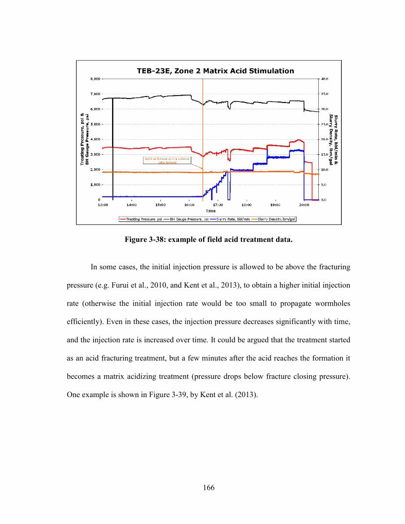
166

Figure 3-38: example of field acid treatment data. In some cases, the initial injection pressure is allowed to be above the fracturing

pressure (e.g. Furui et al., 2010, and Kent et al., 2013), to obtain a higher initial injection

rate (otherwise the initial injection rate would be too small to propagate wormholes

efficiently). Even in these cases, the injection pressure decreases significantly with time,

and the injection rate is increased over time. It could be argued that the treatment started

as an acid fracturing treatment, but a few minutes after the acid reaches the formation it

becomes a matrix acidizing treatment (pressure drops below fracture closing pressure).

One example is shown in Figure 3-39, by Kent et al. (2013).

167

Figure 3-39: example of field acid treatment data. As the injection rates change during these operations, to calculate the injection rate

that allows keeping a given pressure (or vice-versa) it is necessary to use the superposition

of the transient solution. Assume a reservoir initially at uniform pressure 𝑝 , where the

injection rate varies in steps 𝑞 , 𝑞 , …, 𝑞 , …, 𝑞 . The injection rate is 𝑞 = 0 before time

𝑡 = 0, and 𝑞 is the injection rate from time 𝑡 = 0 up to time 𝑡 , and so forth (𝑞 is the

injection rate from time 𝑡 up to time 𝑡 ), the bottomhole pressure at the end of the N-th

time step (at time 𝑡 ) is given by:

𝑝 (𝑡 ) = 𝑝 +𝜇𝐵

4𝜋𝑘ℎ𝑞 − 𝑞 𝐸

𝜙𝜇𝑐 𝑟

4𝑘 𝑡 − 𝑡+

𝜇𝐵

2𝜋𝑘ℎ𝑞 𝑠(𝑡 )

(3.78)

168

where 𝐸 is the exponential integral function, and 𝑠(𝑡 ) is the skin factor at time 𝑡 . Due

to wormhole propagation, this skin factor decreases with time. If the injection rate is kept

constant, in theory, the bottomhole pressure may increase or decrease with time, due to

the combined effect of transient flow and wormhole propagation. In equation (3.78), the

summation term increases with time, but 𝑠(𝑡 ) decreases with time. Figure 3-39 shows an

example of pressure decreasing with time, even for an increasing injection rate.

Equation (3.78) can be used in different ways. One is to calculate the skin factor

in real time during acid treatments, using measured 𝑝 (𝑡) and known injected 𝑞 (𝑡), to

evaluate the treatment progress (such as the method proposed by Zhu and Hill, 1998).

Another use of equation (3.78) is to estimate, in a design phase, what is the maximum

injection rate that can be injected at a given well to keep the pressure below a desired

value. For example, to have bottomhole pressure equal to 𝑝 , at time 𝑡 , the injection

rate 𝑞 can be isolated from equation (3.78) to give:

𝑞 ≤

4𝜋𝑘ℎ𝜇𝐵

𝑝 , − 𝑝 + 𝑞 𝐸𝜙𝜇𝑐 𝑟

4𝑘(𝑡 − 𝑡 )− ∑ 𝑞 − 𝑞 𝐸

𝜙𝜇𝑐 𝑟

4𝑘 𝑡 − 𝑡

𝐸𝜙𝜇𝑐 𝑟

4𝑘(𝑡 − 𝑡 )+ 2𝑠(𝑡 )

(3.79)

The exponential integral function, 𝐸 (𝑥) is available in most commercial

calculation software and spreadsheets, but it can be simplified by 𝐸 (𝑥) ≈ − ln(𝑒 𝑥)

when 𝑥 < 0.01, where 𝛾 is Euler-Mascheroni constant, with 𝑒 ≈ 1.781.

Equation (3.79) can be used to estimate the stepwise injection rate as a function of

time that can injected to keep the bottomhole pressure at 𝑝 , . For each time step, the

169

wormhole propagation is calculated using the corresponding injection rate, and the skin

factor is updated. We can call the injection rate calculated with equation (3.79) by

𝑞 (𝑡), as it is the maximum allowable injection rate to not have a pressure higher than

𝑝 , . If desired, the injection rate 𝑞 (𝑡) calculated with equation (3.79) can be

compared to the optimal injection rate 𝑞 (𝑡) from equation (3.77). If 𝑞 > 𝑞 , the

engineer may choose to inject at a smaller rate, closer to 𝑞 , in which case the bottomhole

pressure would be smaller than 𝑝 , . However, it should be remembered that an

injection rate higher than 𝑞 is always preferable than a rate smaller than 𝑞 .

The method is illustrated in Figure 3-40, for a matrix acidizing treatment with 1

bbl/ft of 15% HCl in a vertical well, in a 500 ft thick formation of 10 md permeability,

with an initial damage skin factor of 9. The breakdown pressure is 𝑝 = 7,000 𝑝𝑠𝑖, and

the maximum allowable pressure is set to 300 psi less than that, 𝑝 , = 6,700 𝑝𝑠𝑖. The

injection rate is calculated with equation (3.79) in time steps, so that the bottomhole

pressure does not exceed 𝑝 , . Initially, the injection rate must be small because of the

positive skin factor due to formation damage. As the damage is bypassed by the

wormholes, the pressure decreases significantly over the first time steps, allowing the

injection rate to be increased. After the damage has been completely bypassed and the

wormholes are a few feet long, the pressure becomes more stable, and the injection rate

varies less with time. The example of injection rate shown in Figure 3-40, calculated with

equation (3.79), is similar to the field cases shown in Figure 3-38 and Figure 3-39. The

surface pressure may look very different from the bottomhole pressure, because the

frictional pressure drop is approximately proportional to the injection rate squared.

170

Figure 3-40: example of synthetic matrix acidizing treatment, 10 md If the permeability is high enough to allow high injection rates, the maximum

injection rate may be limited by equipment (pump maximum pressure or power, maximum

surface pressure, etc). In these cases, even injecting at the maximum injection rate, the

bottomhole pressure does not reach the maximum allowable value. An example of this

behavior is shown in Figure 3-41, for a reservoir of 60 md, where a maximum allowable

injection rate was set to 60 bpm. All other properties are the same as those that generated

Figure 3-40, except for the permeability. Initially, the injection rate starts around 30 bpm,

and pressure increases up to the maximum allowable. But as soon as the formation damage

is bypassed by the wormholes, pressure declines enough that the injection rate is increased

to the maximum set to 60 bpm. After some time, the bottomhole pressure decreases due

to wormhole propagation, being below the maximum allowable value. Similar behavior

happens in the field example shown in Figure 3-39.

171

Figure 3-41: example of synthetic matrix acidizing treatment, 60 md In both previous examples, the permeability is high enough (10 and 60 md) so that

the injection rate is above the optimal injection rate throughout the whole treatment. This

is illustrated in Figure 3-42a for the 10 md case. For smaller permeabilities, however, it

may not be possible to inject at the optimal injection rate, as illustrated in Figure 3-42b,

for a reservoir of 1 md (all properties are the same as the previous examples, except for

permeability).

172

(a) 10md (b) 1 md

Figure 3-42: comparison of the maximum and optimal injection rate for (a) 10 md and (b) 1 md

Because of the maximum allowable injection pressure, in low permeability

reservoirs it may not be possible to inject at the optimal injection rate that would lead to

dominant wormhole propagation. This makes the outcome of matrix acidizing treatments

in low permeability reservoirs significantly impaired. Figure 3-43 shows the resulting

dimensionless productivity index of matrix acidized wells for permeability ranging from

0.01 md to 1,000 md. All other properties are the same of the previous examples.

173

Figure 3-43: example dimensionless productivity index of matrix acidized wells As can be seen in Figure 3-43, if the permeability is too small, matrix acidizing

may not even be able to remove the formation damage because the injection velocity is

not high enough to propagate wormholes. In this particular example, a permeability of at

least 0.2 md is required to be able to remove the formation damage with the acid treatment

simulated. There are two different curves plotted, that overlap below 3 md. The blue

continuous curve corresponds to the treatment injected at the maximum injection rate

𝑞 , calculated using equation (3.79). The red dotted curve corresponds to the treatment

injected at optimal injection rate 𝑞 when possible, calculated using equation (3.77).

In this example, bottomhole pressure is not allowed to exceed the maximum

allowable value set as 𝑝 , = 6,700 𝑝𝑠𝑖. At permeabilities below 3 md it is not possible

to inject at 𝑞 without exceeding 𝑝 , . Hence, the curves of 𝑞 and 𝑞 overlap

below 3 md. For permeabilities above 3 md, however, 𝑞 > 𝑞 (such as shown in

174

Figure 3-42a for the 10 md case). In these higher permeabilities, injecting at optimal

injection rate leads to a higher productivity index than injecting at the maximum injection

rate. The difference is not too large, though, because, as mentioned already, the slope of

the 𝑃𝑉 curve is small above the optimal interstitial velocity.

This is the method used in this study, in section 5, to estimate the maximum

productivity of matrix acidized wells and compare it with acid fractured wells.

3.4.1. Theoretical Maximum Productivity of Matrix Acidized Wells

If the permeability is high enough, it is theoretically possible to inject the acid at

the optimal injection rate, that results in the maximum wormhole propagation, leading to

the theoretical maximum possible productivity. In the example shown in Figure 3-43, for

example, this is possible for permeabilities of 3 md or above.

The theoretical maximum possible productivity of a matrix acidized well can be

easily estimated. It is obtained when the longest wormhole length is achieved, which is

obtained with the minimum 𝑃𝑉 value, 𝑃𝑉 , , obtained when the optimal injection

velocity is maintained at the wormhole front. If 𝑃𝑉 , is known, the maximum

wormholed region radius can be estimated using the volumetric model. It can be derived

from the definition of 𝑃𝑉 , using as volume of the rock the volume of the wormholed

region:

175

𝑃𝑉 =𝑉

𝜙𝑉 =

𝑉

𝜙𝜋(𝑟 − 𝑟 )𝐿 (3.80)

where 𝑟 is the radius of the cylindrical wormholed region around the wellbore, 𝑟 is the

wellbore radius, 𝑉 is the volume of the acid solution injected, 𝜙 is the reservoir porosity,

and 𝐿 is the length of the wellbore being acidized. Isolating 𝑟 :

𝑟 = 𝑟 +𝑉

𝜋𝜙𝐿𝑃𝑉

(3.81)

The greatest possible radius of the wormholed region is given by:

𝑟 , = 𝑟 +𝑉

𝜋𝜙𝐿𝑃𝑉 ,

(3.82)

where 𝑃𝑉 , is the minimum value of 𝑃𝑉 , in the field scale, given by equation

(3.39).

The corresponding maximum possible dimensionless productivity index for a

matrix acidized vertical well (in pseudo-steady state in a circular drainage area), is:

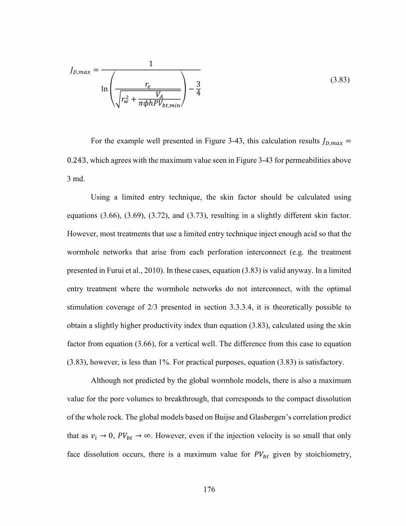
176

𝐽 , =1

ln

⎝

⎛ 𝑟

𝑟 +𝑉

𝜋𝜙ℎ𝑃𝑉 , ⎠

⎞ −34

(3.83)

For the example well presented in Figure 3-43, this calculation results 𝐽 , =

0.243, which agrees with the maximum value seen in Figure 3-43 for permeabilities above

3 md.

Using a limited entry technique, the skin factor should be calculated using

equations (3.66), (3.69), (3.72), and (3.73), resulting in a slightly different skin factor.

However, most treatments that use a limited entry technique inject enough acid so that the

wormhole networks that arise from each perforation interconnect (e.g. the treatment

presented in Furui et al., 2010). In these cases, equation (3.83) is valid anyway. In a limited

entry treatment where the wormhole networks do not interconnect, with the optimal

stimulation coverage of 2/3 presented in section 3.3.3.4, it is theoretically possible to

obtain a slightly higher productivity index than equation (3.83), calculated using the skin

factor from equation (3.66), for a vertical well. The difference from this case to equation

(3.83), however, is less than 1%. For practical purposes, equation (3.83) is satisfactory.

Although not predicted by the global wormhole models, there is also a maximum

value for the pore volumes to breakthrough, that corresponds to the compact dissolution

of the whole rock. The global models based on Buijse and Glasbergen’s correlation predict

that as 𝑣 → 0, 𝑃𝑉 → ∞. However, even if the injection velocity is so small that only

face dissolution occurs, there is a maximum value for 𝑃𝑉 given by stoichiometry,

177

equivalent to the volume of acid required to dissolve the whole rock. For a rock composed

with volume fraction of soluble mineral equal to 𝑓 , with porosity 𝜙, and an acid with

volumetric dissolving power 𝜒, the maximum possible value of 𝑃𝑉 is given by:

𝑃𝑉 , =(1 − 𝜙)𝑓

𝜙𝜒

(3.84)

The volumetric dissolving power, denoted by 𝜒, is defined as the volume of

mineral dissolved by a unit volume of acid solution, given by:

𝜒 =𝛽 𝐶𝜌

𝜌

(3.85)

where 𝐶 is the acid mass fraction of the acid solution, 𝜌 is the density of the acid solution,

and 𝜌 is the density of the dissolved mineral. As an example, for 15% HCl dissolving

calcite, 𝜒 = 0.082 volume of calcite per volume of 15% acid solution, and for 15% HCl

dissolving dolomite 𝜒 = 0.071 volume of dolomite per volume of 15% acid solution.

In a high porosity rock with 𝜙 = 0.35, composed of 100% calcite, injecting 28%

HCl (𝜒 = 0.16), the worst possible value is 𝑃𝑉 , = 11.6. On the other hand, in a low

porosity rock with 𝜙 = 0.08, composed of 100% calcite, injecting 15% HCl (𝜒 = 0.082),

the worst possible value is 𝑃𝑉 , = 140.

In most field cases, this is not important, because acid is injected at the maximum

possible injection rate, which results in a 𝑃𝑉 much smaller than 𝑃𝑉 , . A well-

178

designed matrix acidizing treatment should never be injected at such a low injection rate

as to result in 𝑃𝑉 , . But still, it is interesting to know the worst-case scenario.

Historically, many acid treatments have been pumped using injection rates much smaller

than the optimal, especially when using coiled tubing to treat long intervals. In these cases,

𝑃𝑉 is much greater than 𝑃𝑉 , , but it should still be no greater than 𝑃𝑉 , .

179

4. IMPROVEMENTS IN ACID FRACTURING MODELING *

In this chapter, the state of the art of modeling acid fracturing operations is

discussed. Recent improvements developed in this study are presented, including a new

acid leakoff model that accounts for wormhole propagation and a simulator for calculating

the acid fractured well productivity integrated to a fully-coupled acid fracturing simulator.

Finally, a method to design acid fracturing operations and to estimate the best possible

outcome of acid fracturing operations is presented, as well as a simplified method to

quickly obtain a rough estimate of the best possible outcome of an acid fracturing

operation.

4.1. New Acid Leakoff Model for Acid Fracturing

The classic leakoff model for fracturing operations was first introduced by Carter

(1957), relating the leaking fluid velocity 𝑣 to a leakoff coefficient 𝐶 and to time by:

𝑣 =𝐶

√𝑡 (4.1)

* Part of this section is reprinted with permission from “Aljawad, M. S., Schwalbert, M. P., Zhu, D., & Hill, A. D. (2018b, October 16). Guidelines for Optimizing Acid Fracture Design Using an Integrated Acid Fracture and Productivity Model. Society of Petroleum Engineers. doi:10.2118/191423-18IHFT-MS”

180

Carter’s leakoff model has been used since its publication, assuming a constant

leakoff coefficient 𝐶 . Howard and Fast (1957) decomposed the leakoff coefficient into

three separate components (𝐶 , 𝐶 , and 𝐶 ), caused by three separate mechanisms that

could retard the leakoff velocity. The three mechanisms are: (1) wall-building filter cake

due to additives in the fracturing fluid (𝐶 ), (2) pressure drop in the zone invaded by the

fracturing fluid’s filtrate (𝐶 ), and (3) reservoir compressive resistance (𝐶 ).

The wall-building coefficient 𝐶 can be determined experimentally by a filtration

experiment, while 𝐶 and 𝐶 can be calculated by:

𝐶 =𝜙𝑐 𝑘

𝜋𝜇Δ𝑝

(4.2)

𝐶 =𝜙𝑘Δ𝑝

2𝜇

(4.3)

where 𝜇 is the viscosity of the reservoir fluid, and 𝜇 is the viscosity of the leaking fluid

(filtrate).

The relationship of these different coefficients with time is the same as in Carter’s

model, equation (4.1), and the three coefficients can be combined to result in a total leakoff

coefficient, given by equation (4.9), which still follows equation (4.1).

181

𝐶 =

−1𝐶

+1

𝐶+ 4

1

𝐶+

1

𝐶

21

𝐶+

1

𝐶

(4.4)

Hill et al. (1995) proposed a modification of the calculation of the viscous

component of the leakoff coefficient, 𝐶 , to account for the wormholes. The viscous

component with the wormhole effect is denoted by 𝐶 , , and calculated by:

𝐶 , =𝜙𝑘Δ𝑝

2𝜇 1 −1

𝑃𝑉 ,

=𝑃𝑉 ,

𝑃𝑉 , − 1𝐶 (4.5)

As mentioned in Section 2.3.2, currently available leakoff models do not account

for the high leakoff observed in cases of efficient wormholing, when 𝑃𝑉 ≪ 1. The

leakoff model by Hill et al. (1995) accounts for wormholes, but it is only valid for 𝑃𝑉 >

1, and as 𝑃𝑉 → 1, it predicts 𝐶 , → ∞ and consequently, if there is no filter cake,

𝐶 → 𝐶 . In other words, it predicts that the maximum possible value for the leakoff

coefficient 𝐶 is given by the reservoir compression coefficient 𝐶 given by equation (4.2).

In cases where the wormhole propagation is not efficient, such as weak acids,

reservoirs with low permeability or dolomite mineralogy, the model by Hill et al. (1995)

is valid and its use is encouraged, given its simple and elegant form. This section presents

182

a new acid leakoff model, derived to be valid in cases of efficient wormholing (when

𝑃𝑉 < 1).

Both numerical and analytical models were developed for this end. The numerical

model simulates the flow from the fracture faces into the reservoir and calculates the

wormhole propagation using a global wormhole model, then updates the reservoir

permeability due to the wormholes. The analytical model is more efficient and gives the

same results. The use of the analytical model is encouraged. The numerical model is used

for validation purposes.

4.1.1. Derivation of the New Leakoff Model

The derivation of the new leakoff model starts with the transient diffusivity

equation in one dimension, for constant properties:

𝜙𝜇𝑐

𝑘

𝜕𝑝(𝑦, 𝑡)

𝜕𝑡=

𝜕 𝑝(𝑦, 𝑡)

𝜕𝑦

(4.6)

where 𝑦 is the distance orthogonal to the fracture wall. As this equation is one-

dimensional, linear flow is assumed to occur from the fracture walls. That is a good

assumption close to the fracture walls and far from the tip of the fracture, where a radial

component in the flow exists. As equation (4.6) assumes constant properties, it is valid in

183

the portion of the reservoir untouched by the leaked acid. So it is valid ahead of the

wormholes front.

Equation (4.6) is also used to derive the leakoff coefficient due to the reservoir

fluids compression, coefficient 𝐶 given by equation (4.2). If the initial reservoir pressure

is 𝑝 and the pressure inside the fracture is 𝑝 , this equation can be solved using as

boundary conditions 𝑝(𝑦 = 0) = 𝑝 and 𝑝(𝑦 → ∞) = 𝑝 , and initial condition 𝑝(𝑡 =

0) = 𝑝 . The solution is:

𝑝(𝑦, 𝑡) = 𝑝 − 𝑝 − 𝑝 erf

⎝

⎛𝑦

4𝑘𝑡𝜙𝜇𝑐 ⎠

⎞ (4.7)

Equation (4.7) is plotted in Figure 4-1, for various time steps. The blue line is the

numerical solution simulating the flow from the fracture into the reservoir using the finite

volumes method, and the dotted red line is equation (4.7). This is the pressure field due

only to the reservoir compression, without wormholes. It is important for the comparison

to the case with wormholes, shown in the following.

184

Figure 4-1: pressure field in the reservoir due to leakoff without wormholes (the fracture face is located at y=0).

The velocity at any position is then given by:

𝑣(𝑦, 𝑡) = −𝑘

𝜇

𝜕𝑝

𝜕𝑦

(4.8)

From equation (4.7), the derivative of pressure is given by:

𝜕𝑝

𝜕𝑦= − 𝑝 − 𝑝

𝜕

𝜕𝑦erf

⎝

⎛𝑦

4𝑘𝑡𝜙𝜇𝑐 ⎠

⎞ = − 𝑝 − 𝑝

2 exp −𝑦

4𝑘𝑡𝜙𝜇𝑐

√𝜋4𝑘𝑡

𝜙𝜇𝑐

(4.9)

Joining equations (4.8) and (4.9) and grouping terms:

185

𝑣(𝑦, 𝑡) = −𝑘

𝜇

⎩⎨

⎧

− 𝑝 − 𝑝2

𝜋4𝑘𝑡𝜙𝜇𝑐

exp −𝑦

4𝑘𝑡𝜙𝜇𝑐 ⎭

⎬

⎫

(4.10)

𝑣(𝑦, 𝑡) = 𝑝 − 𝑝𝑘𝜙𝑐

𝜋𝜇𝑡exp

−𝑦 𝜙𝜇𝑐

4𝑘𝑡

(4.11)

If neglecting the wormholes, the velocity at the fracture faces (leakoff velocity) is

given by:

𝑣(𝑦 = 0, 𝑡) = 𝑝 − 𝑝𝑘𝜙𝑐

𝜋𝜇𝑡

(4.12)

Multiplying equation (4.12) by the square root of time, equation (4.2) is obtained

(coefficient 𝐶 , neglecting the wormholes):

𝐶 = 𝑝 − 𝑝𝑘𝜙𝑐

𝜋𝜇

(4.13)

When acid leaks, the fracture face is dissolved, but if the leakoff velocity is near

the optimal velocity for wormhole propagation, wormholes propagate from the fracture

186

face. The wormhole length increases with time, and it is here denoted as 𝑙 (𝑡). As the

wormholed region is highly permeable, the pressure drop from the fracture face up to the

tip of the wormholes is much smaller than the pressure drop that would exist if there were

no wormholes. The wormholes “bypass” a large portion of the reservoir pressure drop.

This can be seen in Figure 4-2, which shows the pressure field in the reservoir with

and without wormholes growing from the fracture face. The dotted red line is the pressure

without wormholes (such as shown in Figure 4-1), and the blue line is the pressure field

with wormholes propagating from the fracture face, obtained by numerical solution of the

flow in the reservoir, using the finite volumes method, calculating the wormhole growth

with a global model, and updating the permeability of the wormholed region to 1,000

times the original reservoir permeability. There is a small pressure drop in the wormholed

region, due to the large (but not infinite) permeability. But as this permeability is so large,

the transient period is negligible in the wormholed region, and Figure 4-2 shows that the

pressure drop in the wormholed region is a straight line (steady state pressure profile in

the wormholed region, even though the simulation is transient).

187

Figure 4-2: pressure field in the reservoir due to leakoff with wormholes propagating (the fracture face is located at y=0).

The pressure drop in the wormholed region can usually be neglected because its

permeability is much larger than the original reservoir permeability. If it is included, it can

be treated as a straight line (Darcy’s law, steady state, linear flow). If the permeability of

the wormholed region is 𝑘 , the viscosity of the fluid that flows through the wormholed

region is 𝜇 , and the leakoff velocity is 𝑣 (𝑡), then the pressure profile from the fracture

face up to the wormhole front is given by:

𝑝(𝑦 ≤ 𝑙 (𝑡), 𝑡) = 𝑝 −𝜇 𝑣 (𝑡)

𝑘𝑦

(4.14)

The pressure at the tip of the wormhole front is given by:

188

𝑝 , (𝑡) = 𝑝(𝑙 (𝑡), 𝑡) = 𝑝 −𝜇 𝑣 (𝑡)

𝑘𝑙 (𝑡)

(4.15)

After the tip, the pressure is still dictated by the diffusivity equation in the

reservoir. However, it is not the original solution, equation (4.7), because the wormhole

propagation continually imposes a high pressure 𝑝 , (𝑡) at the wormhole front. In other

words, the wormhole front is continually imposing a new boundary condition, not at the

fracture face anymore, but at the wormhole front. To find the new solution with

wormholes, the superposition principle can be used.

The superposition principle states that if 𝑦 (𝑥, 𝑡) and 𝑦 (𝑥, 𝑡) are both solutions to

a linear differential equation, then the combination 𝑦 (𝑥, 𝑡) + 𝑦 (𝑥, 𝑡) is also a solution.

If 𝑝 (𝑦, 𝑡) is the solution caused by a boundary condition 𝑝 and 𝑝 (𝑦, 𝑡) is the solution

caused by a boundary condition 𝑝 , then the solution caused by the addition of both

boundary conditions, 𝑝 + 𝑝 , is a combination of 𝑝 (𝑦, 𝑡) and 𝑝 (𝑦, 𝑡), appropriately

shifted in time and space.

In this leakoff problem, the initial boundary condition is simply the fracture

pressure at the fracture face: 𝑝(0,0) = 𝑝 . The solution to this problem is given by

equation (4.7), which can be rewritten in terms of the perturbation in the pressure field:

189

∆𝑝(𝑦, 𝑡) = 𝑝(𝑦, 𝑡) − 𝑝 = 𝑝 − 𝑝

⎣⎢⎢⎡

1 − erf

⎝

⎛𝑦

4𝑘𝑡𝜙𝜇𝑐 ⎠

⎞

⎦⎥⎥⎤

(4.16)

The wormhole front continually propagates. In this study the time is discretized to

find a solution. The continuous wormhole propagation is treated as if it was stepwise: at

each time step ∆𝑡, the wormhole front propagates a distance ∆𝑙 . Starting from the initial

time, 𝑡 = 0, when there is no wormhole, at each time step, 𝑣 (𝑡) is calculated, then used

with a global wormhole model to calculate 𝑙 (𝑡); the procedure proceeds to the next time

step, when the presence of the wormholes at 𝑦 = 𝑙 (𝑡) imposes a new boundary

condition: 𝑝 , (𝑡) = 𝑝(𝑙 (𝑡), 𝑡) = 𝑝 −( )

. At each time step, the

superposition of the solution for 𝑝(𝑦, 𝑡) with this new boundary condition is used with the

solutions for 𝑝(𝑦, 𝑡) from the previous time steps. Each time step adds a term in the

superimposed solution of the pressure field.

All the additions must be made in terms of the perturbation in the previous pressure

field. To have a homogeneous initial condition, the solution is sought in terms of

∆𝑝(𝑦, 𝑡) = (𝑝(𝑦, 𝑡) − 𝑝 ). At the first time step, the previous pressure field is the initial

reservoir pressure, 𝑝(𝑦, 0) = 𝑝 , so the initial condition is ∆𝑝(𝑦, 0) = 0, and the boundary

condition perturbation is ∆𝑝(0,0) = 𝑝 − 𝑝 . In the next time steps, the perturbation

happens at the wormhole front, at 𝑦 = 𝑙 (𝑡), where there is already a pre-existing

pressure larger than 𝑝 due to the pressure diffusion from the previous time steps.

190

In this text, the pre-existing pressure at the wormhole front is called 𝑝 , (𝑡),

where the super-index 𝑝𝑒 stands for “pre-existing”. The pressure imposed by the

wormhole tip is 𝑝 , (𝑡), given by equation (4.15). With this terminology, the

perturbation in the pressure field imposed by the wormhole front at time 𝑡 as a new

boundary condition is given by ∆𝑝(𝑙 (𝑡), 𝑡) = 𝑝 , (𝑡) − 𝑝 , (𝑡) .

The total pressure solution at a given time 𝑡 (the N-th time step) is given by the

combination of the contribution from the perturbation of each time step 𝑗, ∆𝑝 (𝑦, 𝑡). The

first term is the solution without wormholes, called here ∆𝑝 (𝑦, 𝑡), and given by equation

(4.16). At time 𝑡 , the wormhole front is at 𝑦 = 𝑙 (𝑡 ), and its contribution to the total

pressure field is ∆𝑝 (𝑦, 𝑡), given by:

∆𝑝 (𝑦 ≥ 𝑙 (𝑡 ), 𝑡 ≥ 𝑡 ) = 𝑝 , (𝑡 ) − 𝑝 , (𝑡 )

⎩⎨

⎧

1 − erf

⎣⎢⎢⎡[𝑦 − 𝑙 (𝑡 )]

4𝑘(𝑡 − 𝑡 )𝜙𝜇𝑐 ⎦

⎥⎥⎤

⎭⎬

⎫

(4.17)

The shift in space to [𝑦 − 𝑙 (𝑡 )] happens because the new boundary condition

is imposed at 𝑦 = 𝑙 (𝑡 ), and the shift in time (𝑡 − 𝑡 ) happens because this new

boundary condition is only imposed at time 𝑡 = 𝑡 . Accordingly, the contribution of each

time step 𝑗, at time 𝑡 , is ∆𝑝 (𝑦, 𝑡), given by:

191

∆𝑝 𝑦 > 𝑙 𝑡 , 𝑡 ≥ 𝑡 = 𝑝 , 𝑡 − 𝑝 , 𝑡

⎩⎪⎨

⎪⎧

1 − erf

⎣⎢⎢⎢⎢⎡

𝑦 − 𝑙 𝑡

4𝑘(𝑡 − 𝑡 )𝜙𝜇𝑐

⎦⎥⎥⎥⎥⎤

⎭⎪⎬

⎪⎫

(4.18)

The total combination at time 𝑡 is given by:

∆𝑝(𝑦 > 𝑙 (𝑡 ), 𝑡 ≥ 𝑡 ) =

⎩⎪⎪⎨

⎪⎪⎧

𝑝 , 𝑡 − 𝑝 , 𝑡

⎩⎪⎨

⎪⎧

1 − 𝑒𝑟𝑓

⎣⎢⎢⎢⎢⎡

𝑦 − 𝑙 𝑡

4𝑘(𝑡 − 𝑡 )𝜙𝜇𝑐

⎦⎥⎥⎥⎥⎤

⎭⎪⎬

⎪⎫

⎭⎪⎪⎬

⎪⎪⎫

(4.19)

Hence, the total superimposed pressure field at time step 𝑡 is:

𝑝(𝑦 > 𝑙 (𝑡 ), 𝑡 ≥ 𝑡 ) = 𝑝 +

⎩⎪⎪⎨

⎪⎪⎧

𝑝 , 𝑡 − 𝑝 , 𝑡

⎩⎪⎨

⎪⎧

1 − 𝑒𝑟𝑓

⎣⎢⎢⎢⎢⎡

𝑦 − 𝑙 𝑡

4𝑘(𝑡 − 𝑡 )𝜙𝜇𝑐

⎦⎥⎥⎥⎥⎤

⎭⎪⎬

⎪⎫

⎭⎪⎪⎬

⎪⎪⎫

(4.20)

where 𝑡 = 0, 𝑙 (𝑡 ) = 0, 𝑝 , (𝑡 ) = 𝑝 , 𝑝 , (𝑡 ) = 𝑝 , and:

𝑝 , 𝑡 = 𝑝 −𝜇 𝑣 𝑡

𝑘𝑙 (𝑡 )

(4.21)

192

𝑝 , (𝑡 ) = 𝑝 +

⎩⎪⎪⎨

⎪⎪⎧

𝑝 , 𝑡 − 𝑝 , 𝑡

⎩⎪⎨

⎪⎧

1 − erf

⎣⎢⎢⎢⎢⎡

𝑙 (𝑡 ) − 𝑙 𝑡

4𝑘(𝑡 − 𝑡 )𝜙𝜇𝑐

⎦⎥⎥⎥⎥⎤

⎭⎪⎬

⎪⎫

⎭⎪⎪⎬

⎪⎪⎫

(4.22)

The length of the wormholed region 𝑙 must be updated at each time step. For

this, a wormhole model is necessary, such as the new model presented in section 3.2 or

the models by Buijse and Glasbergen (2005) or Furui et al. (2010). The acid interstitial

velocity, 𝑣 , is required by the wormhole models. In this case, the interstitial velocity is

equal to the leakoff velocity 𝑣 divided by the rock porosity, and it varies with time.

Representing here the wormhole model as a function of the interstitial velocity as 𝑣 (𝑣 ),

such as equation (3.28), the interstitial velocity and length of the wormholed region are

given by:

𝑣 (𝑡) =𝑣 (𝑡)

𝜙

(4.23)

𝑙 𝑡 = 𝑙 𝑡 + 𝑣 (𝑣 ) × 𝑡 − 𝑡

(4.24)

The leakoff velocity 𝑣 (𝑡) can be calculated by the already known pressure field

and Darcy’s law at the wormhole front:

𝑣 (𝑡) = −𝑘

𝜇

𝜕𝑝

𝜕𝑦( )

(4.25)

193

The following derivative is useful for this derivation:

𝜕

𝜕𝑥erf

𝑥 − 𝑎

𝑏=

2

𝑏√𝜋exp −

𝑥 − 𝑎

𝑏

(4.26)

Applying equation (4.26) to equation (4.20), then substituting in equation (4.25)

leads, finally, to the expression for the leakoff velocity 𝑣 :

𝑣 (𝑡 ) =𝜙𝑐 𝑘

𝜋𝜇

𝑝 , 𝑡 − 𝑝 , 𝑡

(𝑡 − 𝑡 )exp −

𝑙 (𝑡 ) − 𝑙 𝑡 𝜙𝜇𝑐

4𝑘(𝑡 − 𝑡 )

(4.27)

The leakoff coefficient including the effect of the wormholes is given by:

𝐶 (𝑡) = 𝐶 , (𝑡) = 𝑣 (𝑡)√𝑡

(4.28)

The calculation of the length of the wormholed region requires knowledge of the

leakoff velocity for equations (4.23) and (4.24). To calculate the leakoff velocity with

equation (4.27), the length of wormholed region is also required. To calculate both 𝑣 and

𝑙 at each time step, some iterative procedure is required. The convergence is easy, and

the leakoff velocity of the previous time step is a good initial guess for all tested cases.

Summarizing, the leakoff coefficient with efficient wormhole propagation is not a

constant value, but varies with time. For calculating it, time must be discretized in small

194

time steps, and, at each time step, the following procedure must be performed: calculate

the length of the wormholed region using equations (4.23) and (4.24) and a suitable

wormhole model, calculate 𝑝 , and 𝑝 , with equations (4.21) and (4.22), calculate

𝑣 with equation (4.27), iterate until convergence of 𝑣 and 𝑙 , and finally calculate 𝐶

with equation (4.28). Figure 4-3 shows an algorithm for the usage of the new leakoff

model.

Figure 4-3: algorithm of new leakoff model with wormhole propagation.

This leakoff coefficient, 𝐶 , is the total leakoff coefficient if there is no filter cake

and negligible resistance in the invaded zone (which is the case if 𝑃𝑉 < 1). It can be

seen as a modification of the compressive component of the leakoff coefficient, 𝐶 , due to

195

the existence of the wormholes. In this sense, we can denote it as 𝐶 , , as written in

equation (4.28).

4.1.2. Validation of the New Leakoff Model

The proposed analytical leakoff model was validated by comparing its prediction

with numerical simulations of the same problem using the finite volumes method. Figure

4-4 shows the comparison for a case of extremely inefficient wormholing (𝑃𝑉 , =

1000). Figure 4-4a shows the leakoff velocity versus time, while Figure 4-4b shows the

leakoff coefficient versus time. In both cases, three curves are plotted: the classical Carter

leakoff coefficient 𝐶 predicted by equation (4.2), the result of the analytical model

proposed in this section, and the result of the numerical simulation using the finite volumes

method. As in this case the wormholing is extremely inefficient (𝑃𝑉 , = 1000),

practically no wormholes are formed, and, as expected, all three curves are overlapped.

This illustrates that for the cases of inefficient wormholing, the proposed model calculates

𝐶 = 𝐶 .

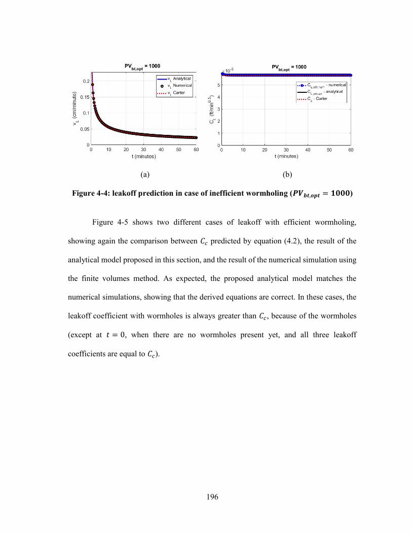
196

(a) (b)

Figure 4-4: leakoff prediction in case of inefficient wormholing (𝑷𝑽𝒃𝒕,𝒐𝒑𝒕 = 𝟏𝟎𝟎𝟎) Figure 4-5 shows two different cases of leakoff with efficient wormholing,

showing again the comparison between 𝐶 predicted by equation (4.2), the result of the

analytical model proposed in this section, and the result of the numerical simulation using

the finite volumes method. As expected, the proposed analytical model matches the

numerical simulations, showing that the derived equations are correct. In these cases, the

leakoff coefficient with wormholes is always greater than 𝐶 , because of the wormholes

(except at 𝑡 = 0, when there are no wormholes present yet, and all three leakoff

coefficients are equal to 𝐶 ).

197

(a)

(b)

Figure 4-5: leakoff prediction in two cases of efficient wormholing.

Figure 4-5a and Figure 4-5b differ in the values of 𝑃𝑉 , and 𝑣 , . The values

of 𝑃𝑉 , and 𝑣 , shown in these figures are in the field scale. Figure 4-5a shows a

higher leakoff coefficient, because it consists of a case of more efficient wormholing

(smaller 𝑃𝑉 , ). Figure 4-5b shows an interesting behavior where the leakoff coefficient

increases initially, and after reaching a maximum around 12 minutes, it starts decreasing.

The reason for this behavior is the decreasing value of the leakoff velocity; initially, the

leakoff velocity is above the optimal velocity for the wormhole propagation (𝑣 >

𝜙𝑣 , ), and the wormholing is more efficient; after some time, as the leakoff velocity

decreases, it becomes smaller than the optimal velocity for wormhole propagation (𝑣 <

𝜙𝑣 , ), hence the wormhole propagation slows down considerably and the leakoff

coefficient decreases, approaching 𝐶 again.

198

4.1.3. Dimensional Analysis of the Wormhole Effect on Leakoff

Dimensional analysis is a useful tool to better understand a given phenomenon.

Based on the proposed analytical model for the acid leakoff coefficient with wormholes,

a few dimensionless numbers arise:

Φ = 𝑃𝑉 , (4.29)

Φ =𝑣

𝜙𝑣 , (4.30)

Φ =𝑙 (𝑡)

4𝑘𝑡𝜙𝜇𝑐

(4.31)

The effect of the first dimensionless number, Φ = 𝑃𝑉 , , is straightforward:

the smaller 𝑃𝑉 , , the more efficient the wormhole propagation, hence the higher the

leakoff. The effect of the second dimensionless number, Φ =,

, is also

straightforward: dominant wormholes propagate when 𝑣 = 𝜙𝑣 , , so the closer Φ is

to 1, the more efficient the wormhole propagation, hence the higher the leakoff. In other

words, if 𝑃𝑉 , is large or 𝑣 ≪ 𝜙𝑣 , , the impact of the wormholes in the acid leakoff

is small.

199

The third dimensionless number arises from the analysis of equation (4.7): as the

pressure drop in the wormholed region is negligible, the pressure drop bypassed by the

wormholes is given by:

∆𝑝 = 𝑝 − 𝑝 erf

⎝

⎛𝑙 (𝑡)

4𝑘𝑡𝜙𝜇𝑐 ⎠

⎞ (4.32)

The importance of the wormholes in leakoff process can be analyzed in terms of

the argument of the error function in equation (4.32), which is the third dimensionless

number Φ . However, as 𝑙 (𝑡) is a function of time and there is time in the denominator

of Φ , this dimensionless number is not a constant. This analysis is simplified if this

dimensionless number is rewritten in a way to eliminate time.

The dependence of 𝑙 (𝑡) with time depends on the wormhole model. Dominant

wormholes propagate when 𝑣 = 𝜙𝑣 , , , where 𝑣 , , is the optimal interstitial

velocity for wormhole propagation in the field scale (as discussed in section 3.2). If the

global wormhole model proposed in section 3.2 is used for the leakoff estimation (linear

flow, scale larger than the representative scales 𝑑 , and 𝑑 , ), the field scale

𝑃𝑉 , , and 𝑣 , , are given by:

𝑃𝑉 , , = 𝑃𝑉 , , ×𝑑

𝑑 ,

(4.33)

200

𝑣 , , = 𝑣 , , ×𝑑

𝑑 ,

(4.34)

The leakoff velocity 𝑣 (𝑡) is a function of time, and with wormholes it should be

always greater than its value without wormholes, given by equation (4.12). The leakoff

velocity with wormholes is larger than what is given by equation (4.12), but on the same

order of magnitude. So the order of magnitude of 𝑙 (𝑡) is given by:

𝑙 (𝑡) = 𝑣 (𝑡)𝑑𝑡 ~𝑣 (𝑡)

𝜙𝑃𝑉 , ,𝑑𝑡 =

𝑝 − 𝑝

𝜙𝑃𝑉 , ,2

𝑘𝜙𝑐 𝑡

𝜋𝜇

(4.35)

Equation (4.35) does not give the exact value of 𝑙 (𝑡), but its order of magnitude.

There are 2 approximate assumptions in its development: (1) that the leakoff velocity is

near the optimal velocity for wormhole propagation, and (2) that the leakoff velocity

follows equation (4.12), which neglects the existence of wormholes in the leakoff. The

first assumption tends to overestimate the wormhole length, while the second tends to

underestimate it. When both assumptions are used simultaneously, the errors in them

partially cancel each other, and the order of magnitude of 𝑙 (𝑡) is correctly predicted by

equation (4.35). Substituting equation (4.35) in (4.31):

201

Φ =𝑙 (𝑡)

4𝑘𝑡𝜙𝜇𝑐

~

2 𝑝 − 𝑝𝑃𝑉 , ,

𝑘𝑐 𝑡𝜋𝜙𝜇

4𝑘𝑡𝜙𝜇𝑐

=𝑐 𝑝 − 𝑝

𝑃𝑉 , , √𝜋

(4.36)

This is a more useful form of the dimensionless number, because it does not

depend on time. In fact, with only four parameters of the reservoir and the fracturing

operation (𝑐 , 𝑃𝑉 , , , 𝑝 , and 𝑝 ), the importance of the wormholes on the leakoff

coefficient can be evaluated. In this work, this dimensionless number is called the “number

of leakoff with wormholes”, and denoted by 𝑁 :

𝑁 =𝑐 𝑝 − 𝑝

𝑃𝑉 , , √𝜋

(4.37)

It is important to notice that 𝑃𝑉 , , is the value of 𝑃𝑉 , in the field scale,

which can be calculated by equation (4.33). It is usually considerably smaller than that

measured in core flooding experiments with small cores (as discussed in section 3.2).

The order of magnitude of the pressure drop bypassed by the wormholes is given

by erf (𝑁 ). The larger the number 𝑁 , the more significant are the wormholes in the

leakoff. If the value of 𝑁 is very small, the wormholes’ impact on leakoff is negligible.

If 𝑁 ~0.01, the order of magnitude of the pressure drop bypassed by the

wormholes is 1%, and the leakoff is expected to increase on the order of 1% because of

the wormholes. If 𝑁 ≲ 0.01, it can be said that the wormholes have negligible effect

202

on leakoff. As 𝑁 increases, however, the importance of the wormholes increases. A

value of 𝑁 ≳ 0.4 can be considered large.

As usually the product 𝑐 𝑝 − 𝑝 is small, this analysis leads to the conclusion

that the wormholes are only important to cause a leakoff coefficient greater than 𝐶 when

𝑃𝑉 , , ≪ 1. As examples, in the cases shown in Figure 4-4, Figure 4-5a, and Figure

4-5b, respectively, 𝑁 = 0.000034 (negligible impact of wormholes on leakoff),

𝑁 = 0.68 (large impact of wormholes on leakoff), and 𝑁 = 0.34 (some impact of

wormholes on leakoff).

Notice that the permeability does not appear in equation (4.37). This does not mean

that permeability is not important in leakoff. In fact, permeability is of major importance

in leakoff. As can be seen in equation (4.27), the leakoff rate is proportional to the square

root of permeability. However, this is also seen in equations (4.12) and (4.13), which do

not account for the wormholes. This means that permeability is very important for leakoff

regardless of the existence of wormholes. A higher leakoff is expected in reservoirs of

higher permeability, but not because of the wormholes.

Notice that the leakoff coefficient predicted by the proposed model is always on

the order of magnitude of 𝐶 . In Figure 4-4, where wormholing is inefficient, this model

predicts 𝐶 = 𝐶 . In Figure 4-5a, where wormholing is efficient, this model predicts that

𝐶 increases with time until more than four times 𝐶 at 30 minutes. It is still on the order

of magnitude of 𝐶 . If 𝑁 is large, 𝐶 may be several times greater than 𝐶 . However,

in reservoirs of low permeability, 𝐶 is small, hence the leakoff is expected to be small;

even if 𝑁 is large, if 𝐶 is small, then the leakoff may still be small.

203

A large value of 𝑁 means the wormholes’ impact on leakoff is significant in

comparison with the value of 𝐶 predicted by equation (4.13). However, if 𝐶 is small to

start with, the value of 𝐶 with the wormholes is probably small too.

This model was developed for cases of 𝑃𝑉 < 1, and because of that the leakoff

coefficient 𝐶 is only compared to the compressive coefficient 𝐶 , and it predicts 𝐶 ≥ 𝐶 .

Because 𝑃𝑉 < 1, the invaded region is fully wormholed, and there is no resistance to

flow in the invaded region (𝐶 → ∞). It is also assumed in this derivation that there is no

filter cake. If fluid loss additives that can block wormholes are used, it is reasonable to

combine a wall building coefficient, 𝐶 , with the leakoff coefficient obtained by this

model. By analogy with the classical leakoff model by Howard and Fast (1957), if the

leakoff coefficient due only to the reservoir compression with wormholes calculated with

equations (4.21) through (4.28) is denoted by 𝐶 , , then the total leakoff coefficient

combined with the filter cake is:

𝐶 =

−1

𝐶 ,+

1

𝐶 ,

+4

𝐶

2

𝐶

(4.38)

This equation always results a total leakoff coefficient that is smaller than the

smaller between 𝐶 , and 𝐶 .

Because the model proposed in this text was developed for 𝑃𝑉 < 1, it always

predicts 𝐶 ≥ 𝐶 , and the previous analysis of the value of 𝑁 refers to the impact of

204

the wormholes in the comparison of how much 𝐶 , is greater than 𝐶 (not considering

filter cake). However, when 𝑃𝑉 > 1, this model can still predict 𝐶 , , but in this case

the effect of the viscous pressure drop of the filtrate invaded zone may be significant. The

corresponding viscous leakoff coefficient component for the invaded zone can be

calculated with the model by Hill et al. (1995), equation (4.5).

This viscous component of the leakoff coefficient with wormholes, 𝐶 , , can be

combined with the compressive component with wormholes, 𝐶 , , calculated with the

model proposed in this text, equations (4.21) through (4.28). Combined still with the filter

cake wall-building coefficient, 𝐶 , the total leakoff coefficient is given by:

𝐶 =

−1

𝐶 ,+

1

𝐶 ,

+ 41

𝐶 ,

+1

𝐶

21

𝐶 ,

+1

𝐶

(4.39)

If the viscous resistance in the invaded zone is negligible, 𝐶 , → ∞. This is the

case, for example, when 𝑃𝑉 < 1, and equation (4.39) reduces to equation (4.38). If the

filter cake resistance is negligible, 𝐶 → ∞, which is the case if the fluid does not form a

filter cake, such as straight acid. If both the viscous resistance and the filter cake resistance

are negligible, 𝐶 , → ∞ and 𝐶 → ∞, and 𝐶 = 𝐶 , .

As mentioned above, previous analysis of the dimensionless 𝑁 refers to the

impact of the wormholes in the comparison of how much 𝐶 is greater than 𝐶 , for a case

205

of no filter cake and 𝑃𝑉 < 1. In other words, it refers to the impact of the wormholes on

𝐶 , compared to 𝐶 . However, even if 𝑃𝑉 > 1, the analysis performed by Hill et al.

(1995) shows that the wormholes can have a significant impact on the total leakoff

coefficient, if the viscous coefficient 𝐶 is significant compared to the compressive

coefficient 𝐶 . In this case, however, 𝐶 is probably not greater than 𝐶 , and the impact of

the wormholes is in the coefficient 𝐶 , , when compared to 𝐶 . In other words, if 𝑃𝑉 >

1, the wormholes may result in 𝐶 , being much greater than 𝐶 . However, the total

leakoff coefficient 𝐶 is not greater than 𝐶 unless 𝑁 is large.

Hill et al. (1995) proposed a dimensionless number denoted by 𝑅 to measure how

important the viscous fluid-loss coefficient 𝐶 is relative to the compressive fluid-loss

coefficient 𝐶 . The dimensionless 𝑅 is defined as the square of the ratio between 𝐶 and

𝐶 (without wormholes effect):

𝑅 =𝐶

𝐶=

2

𝜋

𝜇

𝜇𝑐 ∆𝑝

(4.40)

where 𝜇 is the viscosity of the filtrate in the invaded zone and 𝜇 is the viscosity of the

reservoir fluid.

A large value of 𝑅 means that the resistance of the invaded zone to fluid loss is

large compared to the reservoir compressive resistance, not accounting for wormholes. In

other words, a large value of 𝑅 means that the impact of the wormholes can be significant

just by reducing the resistance of the invaded zone, causing 𝐶 , to be greater than 𝐶 .

206

Interestingly, 𝑅 proposed by Hill et al. (1995) is very similar to 𝑁 proposed in

this study, equation (4.37), in the sense that both are linearly proportional to the product

𝑐 ∆𝑝. Both 𝑅 and 𝑁 depend linearly on the reservoir compressibility and pressure

difference between fracture and reservoir. The difference is that 𝑅 measures the impact

of the viscous leakoff coefficient 𝐶 in comparison with the compressive leakoff

coefficient 𝐶 , and 𝑁 measures the impact of the wormholes in 𝐶 itself, causing the

compressive leakoff coefficient with wormholes, 𝐶 , , to be greater than the reservoir

compressive leakoff coefficient without wormholes, 𝐶 .

Summarizing, a large value of 𝑅 (proposed by Hill et al., 1995) means that the

wormholes can result in a significant increase in leakoff by increasing the viscous

component of the leakoff coefficient, 𝐶 , to 𝐶 , . A large value of 𝑁 means that the

wormholes’ impact on leakoff can cause the compressive component of the leakoff

coefficient with wormholes, 𝐶 , , to be greater than the original reservoir compressive

coefficient without wormholes, 𝐶 .

4.2. Fully-Coupled Acid Fracturing Model

In section 2.3, the available models for simulating acid fracturing treatments were

reviewed. Of particular interest in this study is the model developed in-house in this

research group, because this is the model used in this study, with the modifications

presented in this text. The original model is more detailed in Al Jawad (2018) and Al

207

Jawad et al. (2018a), and it is briefly presented in this text. It was mostly developed by

Murtada Al Jawad, with some contributions of the author.

The acid fracture model consists of a fully coupled model that calculates the

fracture propagation to obtain the fracture geometry, acid transport and reaction, and heat

transfer. At each time step, material balance, and the PKN model along with Liu and Valko

(2015) method for fracture height estimation are used to estimate the fracture geometry.

Then the acid transport equation (4.41) is solved for calculating the acid concentration

distribution inside the created fracture. One of the boundary conditions, equation (4.42),

gives the consumption of acid due to the heterogeneous reaction at the fracture walls, and

from it results the rock dissolution at the fracture walls at each time step. At the same time,

the heat transfer equation is solved for the temperature field, including the heat of reaction

from the heterogeneous reaction at the fracture walls, equations (4.43) and (4.44).

𝜕𝐶

𝜕𝑡+ 𝒗 ∙ ∇𝐶 = ∇ ∙ (𝐷 ∇𝐶)

(4.41)

𝐷 ,

𝜕𝐶

𝜕𝑦= 𝑘 𝐶 − 𝐶 (1 − 𝜙) (4.42)

𝜌 𝐶𝜕𝑇

𝜕𝑡+ 𝜌 𝐶 𝒗 ∙ ∇T = ∇ ∙ (𝜅∇T)

(4.43)

𝜅𝜕𝑇

𝜕𝑦= 𝑘 𝐶 − 𝐶 (1 − 𝜙)∆𝐻 + 𝑞 (𝑡)

(4.44)

The domain for the equations above is the geometry of half of the fracture (one

fracture wing). Symmetry is assumed so that both wings are equal. 𝐶 is acid concentration,

208

𝐷 is the acid diffusivity coefficient, 𝒗 is the acid velocity vector inside the fracture, 𝑦 is

the direction of the fracture width (orthogonal to the direction of fracture propagation), 𝐶

is the acid concentration at the fracture wall (acid-mineral interface), 𝐶 is the acid

concentration at the reaction equilibrium, 𝑘 is the reaction rate pre-exponential

coefficient, 𝑛 is the order of the reaction rate, 𝜌 is the acid solution density, 𝐶 is the

acid solution heat capacity, 𝑇 is temperature, 𝜅 is the acid solution thermal conductivity,

∆𝐻 is the heat of reaction, and 𝑞 is the heat flux from the reservoir.

Figure 4-6 shows a flowchart by Al Jawad et al. (2018b) for the fully-coupled acid

fracturing model. Notice that the three submodels – geometry, acid, and temperature – are

applied both during injection time and after shut-in. Appropriate boundary conditions are

used for different time periods. In addition, the leakoff submodel calculates reactive

leakoff (different from Al Jawad, 2018, the acid leakoff in this study was calculated as

presented in section 4.1), and the fracture conductivity model generates the conductivity

profile after closure. The well productivity model was developed in this work, and it is

presented in section 4.3.

209

Figure 4-6: Flowchart of the acid fracturing model The method presented by Al Jawad et al. (2018a) is used to deal with multiple fluid

stages (e.g. pad, acid, and flush). The model assumes a plug-flow (piston-like)

displacement of each fluid by the subsequent fluids. The effects of possible fingering are

not considered. Each fluid may have a different leakoff coefficient, and the model

calculates a different half-length of the fracture occupied by each fluid. For example, if

there are 3 different fluids, with leakoff coefficients 𝐶 , 𝐶 , and 𝐶 , where fluid 1 is

injected first, then is displaced by fluid 2, which is in turn displaced by fluid 3, the

geometry of the fracture is illustrated in Figure 4-7 (by Al Jawad, 2018).

210

Figure 4-7: fracture geometry with 3 fluid systems

Fluids 1, 2, and 3 occupy the half-lengths 𝑥 , 𝑥 , and 𝑥 in the fracture, where

the total fracture half-length is 𝑥 = 𝑥 + 𝑥 + 𝑥 . Al Jawad (2018) presents a method

to estimate the fracture half-length occupied by each fluid system, and the corresponding

equivalent total leakoff coefficient, based on each fluid’s properties and individual leakoff

coefficients.

In this study, the multiple fluids approach presented by Al Jawad (2018) is used,

but with a modification: the new model to calculate the acid leakoff coefficient (section

4.1). In cases of efficient wormholing, this model leads to a higher acid leakoff coefficient,

which causes the fracture half-length occupied by acid to be shorter (𝑥 in Figure 4-7),

even if the total fracture half-length 𝑥 is long due to a long pad stage preceding the acid.

The acid transport and reaction, equations (4.41) and (4.42), are solved only in the acid

domain, not in the whole fracture. Hence, when acid leakoff coefficient is high, the

fracture half-length that is actually stimulated by acid is much shorter than the total

fracture half-length.

211

Figure 4-8 shows the simulation of an acid fracturing operation with two fluid

systems: pad and acid. Pad is injected from the start up to 30 minutes, and acid is injected

from 30 to 60 minutes.

(a) (b)

Figure 4-8: Results of an acid fracturing simulation with 2 fluid systems: pad + acid. (a) Fracture geometry, and (b) equivalent total leakoff coefficient Figure 4-8a shows the fracture half-lengths versus time, where the continuous

black line is the total fracture half-length, the dotted blue line is the length occupied by

pad, and the dashed red line is the half-length occupied by acid. Up to 30 minutes, there

is only pad inside the fracture, so the total half-length is equal to the pad half-length. After

30 minutes, the total fracture half-length is the sum of the pad half-length and the acid

half-length.

The case presented in this picture has a pad with small leakoff coefficient (𝐶 , =

9.4 × 10 𝑓𝑡/𝑚𝑖𝑛 . ), while the acid leakoff coefficient is very high (transient,

calculated according to section 4.1, varying between 9 × 10 and 1.3 × 10 𝑓𝑡/

212

𝑚𝑖𝑛 . ). Because of this, the half-length occupied by acid is much smaller than the half-

length occupied by pad. At the end of the job, pad occupies a fracture half-length of 583

ft, while the acid occupies only a half-length of 88 ft. In fact the total half-length decreases

during acid injection, because the rate of acid injection is smaller than the sum of acid and

pad leakoff. Also, the half-length occupied by pad continually decreases after 30 minutes,

because it continues to leak off during the acid injection.

Figure 4-8b shows the total equivalent leakoff coefficient versus time. After acid

starts to be injected, the leakoff coefficient starts to continually increase. This is the total

equivalent leakoff coefficient of the 2-fluids system, as presented by Al Jawad (2018).

Before 30 minutes, it is equal to the pad leakoff coefficient. After 30 minutes, it accounts

for both the pad still present in the fracture and the acid being injected. It continually

increases for 2 reasons: the acid leakoff coefficient increases with time (section 4.1) and

the length occupied by pad is continually decreasing, while the length occupied by acid is

slowly increasing.

Notice that in this case the equivalent leakoff coefficient never reaches the leakoff

coefficient of the acid, because there is still pad in the fracture in the end of the operation.

In fact, because the fracture length occupied by pad is larger than that occupied by acid,

the total leakoff coefficient is highly influenced by the pad leakoff coefficient, even during

the acid injection. This may be misleading in field treatments. The variable used to

diagnose leakoff in the field is injection pressure, which is influenced by the total

equivalent leakoff coefficient, which accounts for both pad and acid. In the case of Figure

4-8, one would estimate the leakoff coefficient to be no greater than 2.2 × 10 𝑓𝑡/𝑚𝑖𝑛 . ,

213

while the acid leakoff coefficient actually goes up to 1.3 × 10 𝑓𝑡/𝑚𝑖𝑛 . . Because of

this, the stimulated fracture length would be smaller than expected.

In the case presented in Figure 4-8, even though the fracture reached a half-length

of 716 ft after the pad injection, the acid can only etch the fracture surfaces up to 88 ft

from the wellbore. So the actually stimulated fracture half-length is no more than 88 ft. In

reality, the fingering of acid through the pad could enhance somewhat this acid penetration

distance, as well as alternating more acid / pad stages, to push the acid further down the

fracture.

After simulating the whole acid fracturing treatment, the result of this simulator is

a distribution of the etched width along the fracture surface. Using a semi-empirical

correlation for fracture conductivity, such as those by Nierode and Kruk (1973) or Deng

et al. (2012), the conductivity distribution along the fracture surface can be calculated. As

an example, for the case presented in Figure 4-8, the etched width and fracture

conductivity according to Nierode and Kruk (1973) correlation are shown in Figure 4-9.

With this fracture conductivity distribution, the productivity of the acid fractured well can

be calculated. The validation of the acid fracturing model is presented in Al Jawad (2018).

214

(a)

(b)

Figure 4-9: example of fracture etched width and conductivity distribution obtained from an acid fracturing simulation.

4.2.1. Modifications on the Acid Fracturing Model

The fully-coupled acid fracturing model by Al Jawad (2018) was used in this

study, but with some modifications.

First of all, the leakoff model used for the acid system is the one presented in

section 4.1. The previous model (Hill et al., 1995) was maintained as an option in the code,

as well as the option to manually input a leakoff coefficient for each fluid system. In most

simulations presented in this study, however, the leakoff model presented in section 4.1

was used, unless otherwise mentioned.

Second, the domain for the acid solution was changed to be only the fracture region

penetrated by the acid, according to the multiple fluids model. For example, in the case

presented in Figure 4-8, where the total fracture length reached more than 600 ft but the

215

acid penetrated only 88 ft, the modified model solves for the acid transport and reaction

only in the 88 ft. The model as implemented by Al Jawad (2018) solved the acid transport

and reaction for the whole fracture length, regardless of the length penetrated by the acid.

This is especially important in cases of high acid leakoff, where the acid length is much

smaller than the total fractured length, as shown in Figure 4-8.

Third, a correction for the maximum possible volume of dissolved mineral was

implemented, so as to not have a mass of dissolved rock larger than the maximum possible

with the injected acid, accounting for the acid lost due to leakoff. The reason for including

this correction is: in the acid mass balance, the leaked acid is assumed to leak at the wall

concentration, 𝐶 , given by the boundary condition in equation (4.42). For calcite

formations, this wall concentration is practically zero, because the reaction rate is

practically infinite (the kinetics is dominated by mass transfer). Hence, the acid mass

balance calculates that practically no acid is lost due to leakoff.

In reality, however, it is known that there is live (not consumed) acid leaking,

especially in the cases where there is high leakoff and wormhole propagation. If acid

leaked with 𝐶 ≈ 0, it could not propagate wormholes and would not increase leakoff, as

is often reported in the literature (Crowe et al., 1989, Mukherjee and Cudney, 1993,

Settari, 1993, Furui et al., 2010, Aldhayee et al., 2018). The only way the acid can form

wormholes and increase leakoff rate is leaking at a significant concentration. So the

assumption that acid leaks at the wall concentration given by equation (4.42) causes the

model to underestimate the amount of acid lost due to leakoff, thus overestimating the

mass of rock dissolved at the fracture surfaces.

216

The reason for the discrepancy is that the model assumes flow between smooth

parallel plates with uniformly distributed leakoff across the permeable walls, while in

reality the fracture surface is absolutely rough, which increases turbulence and acid

mixing, and leakoff occurs not only distributed through the walls, but also localized in the

wormholes (and possibly natural fractures). The mixing due to roughness and localized

fluid loss points cause the leaking acid to have higher concentration than the practically

null concentration at the walls that results from the model of parallel planes.

To account for the acid lost due to leakoff in this study, a different assumption was

implemented. The acid leaks at a concentration that should be bounded between the wall

concentration 𝐶 (lower bound) and the bulk concentration at that position, 𝐶 defined

in equation (4.45) (upper bound). Equation (4.46) was implemented in this study for the

concentration of the leaking acid.

𝐶 (𝑥, 𝑧) =∫ 𝐶(𝑥, 𝑧)𝑣 (𝑥, 𝑧)𝑑𝑦

∫ 𝑣 (𝑥, 𝑧)𝑑𝑦

(4.45)

𝐶 = (1 − 𝑓 )𝐶 + 𝑓 𝐶 (4.46)

where 𝐶 is the concentration of the leaking acid and 𝑓 is a number between 0 and 1,

input by the user, which determines how much of the bulk acid concentration leaks. The

assumption that acid leaks at the wall concentration corresponds to 𝑓 = 0, while the

assumption that it leaks at the bulk concentration corresponds to 𝑓 = 1.

217

The value 𝐶 is a function of time and the position on the fracture surface, so

𝐶 (𝑥, 𝑧, 𝑡). To calculate the mass of acid lost due to leakoff, 𝑚 , this value must be

integrated over the fracture surface and over time:

𝑚 = 𝜌 𝑣 𝐶 𝑑𝐴 𝑑𝑡 (4.47)

where 𝜌 is the density of the acid solution, and 𝐴 is the fracture surface.

After determining the mass of acid lost due to leakoff, the mass of dissolved

mineral is corrected by correcting the etched width, so that it is limited by the

stoichiometry accounting for the mass of live acid lost due to leakoff. If the acid is injected

at a concentration 𝐶 , injection rate 𝑞 , during a time 𝑡 , the total mass of acid injected is:

𝑚 = 𝜌 𝐶 𝑞 𝑡 (4.48)

As the mass of acid 𝑚 is lost due to leakoff, the mass of acid that actually etches

the fracture surfaces, 𝑚 , and the fraction of the injected acid that is spent etching the

fracture surfaces, 𝑓 , are given by:

𝑚 = 𝑚 − 𝑚 (4.49)

218

𝑓 =𝑚

𝑚 (4.50)

Hence, the maximum volume of rock that can be dissolved at the fracture surfaces,

𝑉 , (where 𝑒 stands for “etched”), is given by stoichiometry as:

𝑉 , =𝛽 𝑚

𝜌 (1 − 𝜙)=

𝜒𝑓 𝑉

(1 − 𝜙)

(4.51)

where 𝛽 is the gravimetric dissolving power of the pure (100%) acid, equation (3.11),

𝜒 is the volumetric dissolving power, equation (3.85), and 𝑉 is the total volume of acid

injected. After executing the acid fracturing simulator, the distribution of etched width 𝑤

is obtained, and the etched volume can be calculated:

𝑉 = 2𝑤 (𝑥, 𝑧)𝑑ℎ𝑑𝑥

(4.52)

When 𝑉 > 𝑉 , due to the not discounting the mass of acid lost to leakoff, the

etched width can be corrected by:

𝑤 , = 𝑤 ,

𝑉 ,

𝑉

(4.53)

This correction preserves the shape of the etched width distribution predicted by

the model by Al Jawad (2018), but discounts the mass of acid lost due to leakoff. More

219

study is required to determine what controls the value of 𝑓 , and which value should be

used for each scenario. The assumptions used by Al Jawad (2018) and Settari (1993)

correspond to 𝑓 = 0. In this study, the value 𝑓 = 1 was used. The choice for this

value is a conservative decision, as it predicts the maximum loss of acid to leakoff. This

choice was influenced by industry practice, where often values of leakoff coefficient larger

than predicted by the usual models are used to match the observed acid fractured lengths

(Settari, 1993), and by several reports of high acid leakoff coefficient caused by wormhole

propagation (Crowe et al., 1989, Mukherjee and Cudney, 1993, Settari, 1993, Furui et al.,

2010, Aldhayee et al., 2018), which could not occur if acid leaked with null concentration.

4.3. Productivity Model for Acid Fractured Wells

The fully-coupled acid fracturing simulator presented in section 4.2 results in a

fracture geometry and conductivity distribution. In this study, a model was developed to

use this fracture geometry and conductivity distribution to estimate the productivity or

injectivity of the acid fractured well. The new model was integrated in the same code of

the acid fracturing simulator presented by Al Jawad (2018) and Al Jawad et al. (2018a).

The output of the acid fracturing simulator is used as input to populate the permeability of

the fracture in the productivity model. This productivity model was developed by the

author and presented for the first time in Al Jawad et al. (2018b).

220

It must be emphasized that the purpose of this model is not to substitute a reservoir

simulator for the analysis of the reservoir, but simply return the productivity index

resulting from the acid fracturing job. Therefore, it simulates only the drainage region of

the given well, in a simple way (a single well model).

The proposed method simulates a rectangular reservoir with a fractured well in the

middle. Due to symmetry, the simulations are done on a quarter of the reservoir domain,

saving computation time. This geometry is illustrated in Figure 4-10.

Figure 4-10: Diagram of the geometry of the fractured-well productivity model

This simplified reservoir model is discretized, with the grid being refined towards

the fracture in the y-direction, and towards the well in the x-direction. In the y-direction,

the smallest grid block is smaller than the fracture width, so that the fracture itself is part

of the reservoir model, as a set of grid blocks with high permeability, calculated from the

conductivity that results from the acid fracture simulator. Figure 4-11 shows an example

221

of a slice (x-y plane) of the mesh used for this model including the fracture and the

reservoir region drained by the fractured-well. The wellbore is in the origin in Figure 4-11.

Figure 4-11: Example of x-y plane of the mesh used for the productivity model.

As the objective is simply calculating a productivity index or skin factor, single

phase calculation with constant fluid properties is sufficient. Using the Finite Volumes

Method, the diffusivity equation is solved for the pressure field in this simplified reservoir

model. A flowchart illustrating the proposed method is shown in Figure 4-12, including

the acid fracturing simulation and the calculation of the productivity index of the acid

fractured well.

222

Figure 4-12: Flowchart illustrating the proposed method for acid fracture productivity calculation.

As the only well in the drainage region is the acid fractured well being analyzed,

it is not regarded as a source or sink term in the reservoir model, but as a boundary

condition. For the single phase case with no sources, the diffusivity equation is given by:

𝛻 ∙ (𝒌 ∙ 𝛻𝑝) = 𝜙𝜇𝑐𝜕𝑝

𝜕𝑡

(4.54)

Different types of boundary conditions were implemented, for simulating different

production modes. The boundary conditions most used at the wellbore are: (1) constant

pressure (𝑝 = 𝑝 ), and (2) constant flow-rate, originating a Neumann boundary

condition:

223

𝜕𝑝

𝜕𝑥= −

𝑞𝐵𝜇

𝑘 𝑤 2ℎ 𝑎𝑡 𝑡ℎ𝑒 𝑤𝑒𝑙𝑙𝑏𝑜𝑟𝑒 (4.55)

where 𝑞 is production rate, 𝑘 𝑤 is the fracture conductivity right at the wellbore-

fracture contact, ℎ is the fracture height at the wellbore-fracture contact, and 𝐵 is

formation volume factor. The inner boundary conditions at 𝑦 = 0 and 𝑥 = 0 (except at

the wellbore) are no-flow because of symmetry. The no-flow boundary condition is

presented as:

𝒏 ⋅ 𝛻𝑝 = 0 (4.56)

where 𝒏 is the normal vector to the boundary surfaces. At the outer boundaries, 𝑥 = 𝑥 /2

and y= 𝑦 /2, two options of boundary conditions were implemented: (1) no-flow –

equation (4.56) – and (2) constant pressure (𝑝 = 𝑝 ). After the initial transient period, the

solution for the case with no-flow at outer boundaries tends to a pseudo-steady state

solution, and the solution for the case with constant pressure at the outer boundaries tends

to a steady state solution, both classical solutions in petroleum production engineering.

The top and bottom boundaries (above and below the reservoir in z-direction) are both no-

flow boundaries, given by Eq. (4.56). The initial condition is simply a known uniform

initial pressure (𝑝 = 𝑝 ).

The calculation procedure consists of solving Eq. (4.54) for the pressure field in

the drainage region of the acid fractured well, and then evaluating the productivity index.

224

This evaluation depends on the production mode selected – the boundary conditions at the

wellbore and outer boundaries. If constant pressure is used as boundary condition at the

wellbore, the production rate varies along time, and can be calculated at any moment by

integrating Darcy’s law velocity over the wellbore area.

The results presented in this study used as boundary conditions the constant flow

rate at the wellbore and no-flow at outer boundaries, so that after the initial transients, the

pseudo-steady state is developed, a more common assumption in petroleum production

engineering, especially in hydraulic fracturing literature (e.g. Economides et al., 2002, and

Meyer and Jacot, 2005). In this case, after solving for the pressure field, the pressure at

the well, 𝑝 , and the average pressure in the drainage region, �̅� – equation (4.57) – , are

determined with time. The productivity index 𝐽 and the dimensionless productivity index

𝐽 , for the pseudo-steady state, are defined by equations (4.58) and (4.59).

�̅� =∫ 𝑝𝑑𝑉

∫ 𝑑𝑉

(4.57)

𝐽 =𝑞

�̅� − 𝑝 (4.58)

𝐽 =𝐵𝜇

2𝜋𝑘ℎ𝐽

(4.59)

225

4.3.1. Validation of the Productivity Model

The productivity model was validated by comparing its results with four different

benchmarks:

(1) the transient analytical solution for fully penetrating, infinite conductivity fracture,

equations (4.60) and (4.61):

𝑝(𝑦, 𝑡) = 𝑝 + 𝑝 − 𝑝 erf

⎝

⎛𝑦

4𝑘𝑡𝜙𝜇𝑐 ⎠

⎞ (4.60)

𝑞(𝑡) = 4𝑥 ℎ 𝑝 − 𝑝𝑘𝜙𝑐

𝜋𝜇𝑡

(4.61)

(2) the analytical solution for 𝐽 for fully penetrating, infinite conductivity fracture in

pseudo-steady state (Meyer and Jacot, 2005): 𝐽 = ;

(3) the 𝐽 for finite conductivity fractures with uniform conductivity in pseudo-steady

state resulting from the correlations presented by Economides et al. (2013) and

Meyer and Jacot (2005); and

(4) the results of the simulations of the reservoir flow with non-uniform fracture

conductivity using another software (the CFD package OpenFOAM, CFD Direct,

2018).

All validation was satisfactory. Figure 4-13a shows a comparison of pressure

profiles given by the analytical solution (dotted line) and the numerical simulation

226

performed in this work (solid line), in various times. As shown in the figure, the numerical

simulation matches perfectly the analytical solution. Figure 4-13b shows the mesh

convergence plot: the error varying the number of grid blocks used in the discretization.

In general, the error is less than 1% when using 100 grid blocks in the x- and y-directions,

and less than 0.1% when using 400 grid blocks in the x- and y-directions. Such an

execution takes only a few seconds on a personal computer.

Figure 4-13: comparison of productivity numerical model with analytical solution. Similar approaches for calculating the acid fracture productivity had already been

presented in the literature, such as in Ben-Naceur and Economides (1988). Aljawad et al.

(2016) used a commercial reservoir simulator for calculating the well productivity. The

improvement of the approach presented in this study is that the productivity model was

built on the same computation code as the acid fracturing model, and the two models are

integrated. Both acid fracturing and productivity simulations are executed in a single run,

so that for every acid fracture simulation a productivity result is immediately obtained.

227

The impact on well productivity caused by any change in the fracturing design parameters

can be immediately known, allowing optimization of the acid fracturing operation.

4.3.2. Wormholes in the Productivity Model

A version of the acid fractured well productivity model that includes the presence

of wormholes arising from the fracture faces was implemented. In this version, the

wormhole length was calculated for each position along the fracture faces. The wormhole

length is larger near the wellbore and decreases far from the wellbore due to the smaller

acid concentration. The wormholes were then included in the productivity model by

attributing a high permeability in the reservoir grid blocks that comprise the wormholed

region.

The results, however, showed that the presence of the wormholes in the acid

fractured well productivity is only important in the cases where the most suitable acid

stimulation method is not acid fracturing, but matrix acidizing (as discussed in section 5).

In low permeability reservoirs, the presence of the wormholes is negligible, for two

reasons: (1) the wormholes are short due to small leakoff velocity, and (2) the fracture is

long, if well designed and executed, making the wormholes less important when compared

to the fracture. In high permeability reservoirs, in which the leakoff is higher and the

wormholes are longer, the impact of the wormholes in acid fractured well productivity

may become significant.

228

Figure 4-14 shows the acid fractured well productivity for a series of synthetic

example cases of deep carbonate reservoirs, where the permeability varies from 0.01 to

300 md.

Figure 4-14: comparison of acid fractured well productivity by including or not the wormholes in the productivity model

As can be seen, the presence of the wormholes in the productivity model is only

significant at high permeabilities. Up to 1 md, the productivity index of the acid fractured

well with or without wormholes differs by less than 1%, and up to 10 md by less than 2%.

For 100 md, however, it differs by 10%, and for 300 md it differs by 15%. However, as

discussed in section 5, for these high permeabilities, the most suitable stimulation method

would be matrix acidizing, and not acid fracturing.

In conclusion, the presence of wormholes in the acid fracture productivity can be

neglected in most cases, except in those cases of high permeability where acid fracturing

is not the most suitable stimulation method.

229

4.4. Acid Fracturing Design and Maximum Productivity Estimation

There are many parameters that can be adjusted in acid fracturing operations: type

of acid system used (straight, gelled, or emulsified acid), concentration, injection rate,

amount of pad, etc. Optimizing an acid fracturing design consists of determining the set

of conditions that results in the most productive acid fractured well. The fully-coupled

acid fracturing simulator (section 4.2) with productivity model (section 4.3) can be used

to perform this optimization. Al Jawad et al. (2018b) presents several case studies of

optimization, for different reservoirs and volumes of acid. This section presents one

example.

The parameters optimized in this case study are the type of acid system, the amount

of pad, and the injection rate. The volume of acid injected is a major design parameter. A

method was proposed in Al Jawad et al. (2018b) to decide the volume of acid. However,

in fact, the stimulated well productivity always increases when the amount of acid

increases. In this sense, the decision on the amount of acid depends on the bigger picture,

such as economical analysis, mechanical constraints (there have been reports of casing

failure related to large amounts of acid injected per perforation, such as Burton et al.,

2018), to avoid contacting gas or water bearing zones, or logistical constraints. In offshore

operations, the volume of acid is often limited to the capacity of the stimulation vessels –

an acid fracturing operation often uses all the acid volume that can be carried by the boat,

or a fraction of that volume if the same boat must treat more than one well before reloading

with acid.

230

Taking this into account, the objective of this section is to optimize the acid

fracturing parameters that result in the optimal productivity for a given volume of acid.

This procedure can then be repeated for different acid volumes, in order to decide, in

conjunction with mechanical and logistical constraints, which is the most suitable volume

for a given well.

The well and reservoir properties of the case study are presented in Table 4-1. The

reaction kinetics parameters and heat of reaction were obtained from Schechter (1992),

and are presented in Table 4-2. Three different acid systems were considered: straight,

gelled, and emulsified acid. These acid systems may have different properties, depending

on the chemical additives types and concentration. The properties used for each acid

system in this study are presented in Table 4-3, and are considered representative of a

reactive acid system (straight acid), retarded system (gelled acid), and very retarded

system (emulsified acid).

Table 4-1: input data used for the optimization in this section

Input Data Field Unit Reservoir/Formation Properties

Reservoir permeability, 𝑘 0.1 md Reservoir porosity, 𝜙 15% Reservoir initial pressure gradient 0.4333 psi/ft Bottomhole flowing pressure gradient (during production) 0.3 psi/ft Minimum horizontal stress gradient 0.6 psi/ft Breakdown pressure gradient 0.7 psi/ft Biot poroelastic coefficient 1 Poisson ratio 0.25 Young’s Modulus 4x106 psi Toughness, 𝐾 1200 psi-inch0.5 Rock Embedment Strength, 𝑆 50,000 psi Mineralogy 100% calcite Formation fluid density, 𝜌 53 lbm/ft3 Reservoir thickness (net pay), ℎ 100 ft Drainage region length in x-direction, 𝐿 3281 ft Drainage region length in y-direction, 𝐿 3281 ft Formation fluid viscosity, 𝜇 1 cp

231

Table 4-1 - Continued Input Data Field Unit

Formation volume factor, 𝐵 1.3 res.bbl/STB Total compressibility, 𝑐 1x10-5 psi-1 Reservoir temperature, 𝑇 212 oF Formation rock density, 𝜌 162.24 lbm/ft3 Formation specific heat capacity, 𝑐 0.2099 Btu(lb.oF) Formation thermal conductivity, 𝑘 0.907 Btu/(hr.ft.oF)

Wellbore Properties Vertical well Wellbore radius, 𝑟 0.3281 ft Inner casing radius, 𝑟 4.0085 inch Outer casing radius, 𝑟 4.3125 inch Overall heat transfer coefficient, 𝑈 0.039 Btu/(hr.ft2.oF) Ambient temperature, 𝑇 77 oF

Mechanical Properties of Layers Above and Below Pay Zone

Poisson ratio 0.25 Young’s Modulus 4x106 psi Toughness, 𝐾 2200 psi-inch0.5 Horizontal Stress 400psi above reservoir’s stress

Acid Properties Density, 𝜌 67 lbm/ft3 Acid initial concentration, 𝐶 15%

Acid volume,𝑉 500 bbl

Filter cake wall-building leakoff coefficient, 𝐶 0 (no filter cake is formed) Spurt loss, 𝑆 0 gal/ft2 Fluid loss multiplier outside pay zone, 𝑓 0.25 Opening time distribution factor, 𝜅 1.5 Acid heat capacity, 𝑐 0.964 Btu/(lbm.oF) Acid thermal conductivity, 𝜅 0.347 Btu/(hr.ft. oF) Acid temperature at injection, 𝑇 80.6 oF

Acid Wormholing Parameters Wormhole model New proposed model (section 3.2) 𝑃𝑉 , , 0.5 𝑣 , , 2 cm/min 𝑑 1 inch 𝜀 0.53 𝜀 0.63 𝑑 3 ft 𝑑 1 ft

Pad Properties Filter cake wall-building leakoff coefficient, 𝐶 0.003 ft/min0.5 Spurt loss, 𝑆 0 gal/ft2 Fluid loss multiplier outside pay zone, 𝑓 0.25 Consistency index, 𝐾 0.0082 lbf-sn/ft2 Rheology Behavior index, 𝑛 0.55

Acid Fracture Conductivity Correlation Correlation used Nierode and Kruk (1973)

Grid Blocks and Time Step Size for Acid Fracturing Simulation Size of x-direction grids, 𝐷𝑋 3.28 ft Number of y-direction grids, 𝑁𝑌 100 Number of z-direction grids, 𝑁𝑍 1 Number of time steps, 𝑁𝑡 60

232

Table 4-2: Reaction kinetics constants and heat of reaction for the reaction between HCl and Calcite / Dolomite (Schechter, 1992)

Mineral 𝒏𝒓 𝒌𝒓𝟎

𝒌𝒈 𝒎𝒐𝒍𝒆𝒔 𝑯𝑪𝒍

𝒎𝟐. 𝒔.𝒌𝒈𝒎𝒐𝒍𝒆𝒔 𝑯𝑪𝒍

𝒎𝟑 𝒂𝒄𝒊𝒅 𝒔𝒐𝒍𝒖𝒕𝒊𝒐𝒏 𝒏𝒓

∆𝑬

𝑹 (𝑲) ∆𝑯𝒓

𝑲𝑱

𝒎𝒐𝒍 𝑯𝑪𝒍

Calcite 0.63 7.314x107 7.55x103 7.5

Dolomite 6.32x10 𝑇

1 − 1.92x10 𝑇 4.48x105 7.9x103 6.9

Table 4-3: Properties of the acid systems. Acid T (oF) n K (lb/ft2.sn) DA(cm2/s) Reference

Straight 84 1 0.00002 1.00E-04 Roberts and Guin (1975)

Gelled 84 0.55 0.0082 8.00E-06 De Rozieres et al. (1994)

Emulsified 83 0.675 0.0066 2.66E-08 De Rozieres et al. (1994)

Acid fracturing operations were simulated with the three acid systems presented

in Table 4-3, for different amounts of pad fluid preceding the acid stage, and injection

rates varying from 5 to 100 bpm. The pad fluid volume considered varied from 0 (no pad)

to the same volume of acid. The different volumes of pad are represented in the following

pictures by the pad number, 𝑁 , defined as the volume of pad divided by the volume of

acid.

Figure 4-15 shows the productivity index of the acid fractured well stimulated with

straight acid, for the whole range of injection rates. Each curve is a different amount of

pad, indicated by the pad number in the legend. Figure 4-16 presents the simulation results

for gelled acid, and Figure 4-17 for emulsified acid.

233

Figure 4-15: productivity index of well acid fractured with straight acid.

Figure 4-16: productivity index of well acid fractured with gelled acid.

234

Figure 4-17: productivity index of well acid fractured with emulsified acid.

Comparing the three plots, it can be seen that in this case the maximum

productivity index achievable is 0.60, obtained with gelled acid, with no pad, and injection

rate of 50 bpm (Figure 4-16). For gelled acid, approximately the same outcome is obtained

for injection rates between 30 and 80 bpm. The productivity index is smaller when pad is

used, and the more pad, the worse the outcome.

For straight acid, the productivity index increases with the injection rate (Figure

4-15). The maximum productivity index achievable using straight acid is 0.56, at the

maximum injection rate tested, 100 bpm, and with a small amount of pad, 𝑁 = 0.1

(meaning a volume of pad equal to 10% of the volume of acid). Interestingly, for this case,

the behavior of the amount of pad inverts depending on the injection rate: at smaller

injection rates, it is better to use more pad, while at higher injection rates, the small volume

of pad is preferred. The fact that the productivity index increases with the injection rate

without a maximum is a consequence of the high reactivity of the straight acid: at small

235

injection rates, it is mostly consumed near the well; at higher rates, some acid reaches

deeper penetrations inside the fracture before being consumed.

For emulsified acid, the maximum achievable productivity index is 0.58, obtained

with no pad, at a small injection rate of 10 bpm (Figure 4-17). Notice that the more retarded

the acid (smaller diffusivity coefficient), the smaller is the optimal injection rate. The

reaction rate of HCl with calcite is practically infinite at reservoir temperatures, so the

reaction is controlled by the acid diffusivity. The more retarded acids are those that have

smaller diffusivity. As can be seen in Table 4-3, the emulsified acid is more retarded than

the gelled acid, which is more retarded than the straight acid. Accordingly, the emulsified

acid’s optimal injection rate (10 bpm) is smaller than the gelled acid’s (50 bpm), which in

turn is smaller than the straight acid’s (100 bpm).

Although the maximum productivity index of 0.6 is achievable only with gelled

acid, similar values can be obtained with the other acid systems (0.56 for straight acid and

0.58 for emulsified acid). However, the conditions at which the optimal results are

obtained with each acid system are very different. For example, if the optimal condition

of the emulsified acid (10 bpm, no pad) is used with the straight acid, a productivity index

of only 0.33 is obtained. For a better comparison, Figure 4-18 shows the best curve of each

acid type in the same plot.

236

Figure 4-18: comparison of productivity index resulting from the three acid types To decide the best volume of acid, the same procedure can be repeated for different

volumes of acid. While Figure 4-18 shows the productivity index for the three acid

systems using 500 bbl of acid, Figure 4-19 and Figure 4-20 show the same for the volumes

of acid of 100 and 1,000 bbl, respectively (all other properties kept constant).

237

Figure 4-19: comparison of productivity index for 100 bbl of acid

Figure 4-20: comparison of productivity index for 1,000 bbl of acid It can be seen that the maximum achievable productivity index increases with the

volume of acid. In all three cases, the optimal conditions are very similar, the best acid

system being gelled acid in all cases. The optimal injection rate increases slightly with the

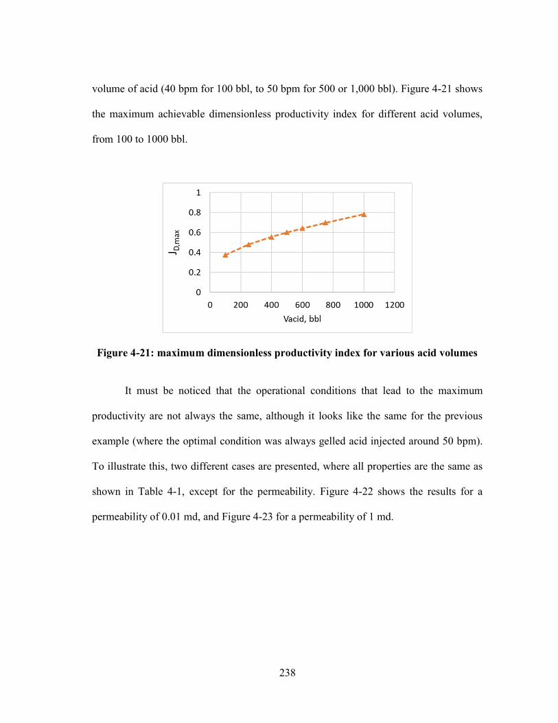
238

volume of acid (40 bpm for 100 bbl, to 50 bpm for 500 or 1,000 bbl). Figure 4-21 shows

the maximum achievable dimensionless productivity index for different acid volumes,

from 100 to 1000 bbl.

Figure 4-21: maximum dimensionless productivity index for various acid volumes It must be noticed that the operational conditions that lead to the maximum

productivity are not always the same, although it looks like the same for the previous

example (where the optimal condition was always gelled acid injected around 50 bpm).

To illustrate this, two different cases are presented, where all properties are the same as

shown in Table 4-1, except for the permeability. Figure 4-22 shows the results for a

permeability of 0.01 md, and Figure 4-23 for a permeability of 1 md.

239

Figure 4-22: acid fractured well productivity for k = 0.01 md

Figure 4-23: acid fractured well productivity for k = 1 md For the reservoir of 0.01 md (Figure 4-22), the best possible acid fracture is

obtained with emulsified acid injected at a very small injection rate, resulting a

dimensionless productivity index of 0.82. For the reservoir of 1 md (Figure 4-23), the

240

optimal operation is achieved with straight acid injected at a very high injection rate (100

bpm), resulting in a dimensionless productivity index of 0.43.

Two important trends can be observed comparing Figure 4-18, Figure 4-22, and

Figure 4-23: (1) for higher permeabilities, less retarded acids are necessary, and (2) for

higher permeabilities, the dimensionless productivity index tends to be smaller.

The first conclusion is explained by the known fact that for higher permeabilities

the optimal fracture length is shorter, so it is not necessary to use retarded acids for the

acid to reach a deeper penetration (the penetration achieved by straight acid is enough).

The second conclusion agrees with the usual industry practice of using hydraulic

fracturing stimulation methods for low permeability reservoirs, and matrix acidizing for

high permeability reservoirs. However, while fractured wells in low permeability

reservoirs have higher dimensionless productivity index (𝐽 ), this does not mean that they

have higher productivity index (𝐽). Although 𝐽 is higher for lower permeabilities, the

productivity index itself (𝐽) is always smaller for less permeable reservoirs.

4.5. Analytical Estimate of Maximum Possible Acid Fractured Well Productivity

The method presented in section 4.4 should be used for design of acid fracturing

operations, to decide the optimal operational conditions: acid system, injection rate,

amount of pad fluid, etc. However, that method can be time consuming, depending on the

number of parameters intended to be tested. Even though the simulation of one operation

241

with the fully-coupled simulator is usually executed in less than a minute on a personal

computer, each point in Figure 4-15 through Figure 4-17 is the result of one such

simulation. If the number of parameters to be tested is large, the total time of all

simulations may become significant.

This section presents a simplified method to quickly estimate the best possible

outcome that can be achieved from acid fracturing, with a given volume of acid.

For propped hydraulic fractured wells in conventional reservoirs, it is a known fact

that there is an optimal fracture length and width that, for a given amount of proppant,

result in the most productive well. This fact was proposed first by Prats (1961), and is

thoroughly explored by Economides et al. (2002), who propose correlations to estimate

the optimal fracture dimensions for a given reservoir. They propose that for each value of

reservoir permeability and volume of proppant, there is an optimal value of dimensionless

fracture conductivity. The dimensionless fracture conductivity 𝐶 is defined as:

𝐶 =𝑘 𝑤

𝑘𝑥 (4.62)

where 𝑘 𝑤 is the fracture conductivity, 𝑘 is the reservoir permeability, and 𝑥 is the

fracture half-length.

The fact that there is an optimal value for 𝐶 , denoted 𝐶 , , means that for a

given volume of proppant there is an optimal compromise between fracture length and

242

width. According to Economides et al. (2002), the value of 𝐶 , is a function of the

proppant number, 𝑁 , defined as:

𝑁 =2𝑘 𝑉

𝑘𝑉

(4.63)

where 𝑉 is the volume of the propped fracture in the pay zone (excluding the possible

volume of proppant lost to non-pay zones), and 𝑉 is the reservoir drainage volume of the

well. If the fracture fully penetrates the pay zone (ℎ = ℎ), the proppant number can be

written as:

𝑁 =4𝑘 𝑤𝑥

𝑘𝐴

(4.64)

where 𝐴 is the drainage area of the well.

According to Economides et al. (2002), the optimal dimensionless fracture

conductivity, in a square drainage region with one bi-wing fracture, is given by:

𝐶 , 𝑁 =

⎩⎪⎨

⎪⎧

1.6 𝑖𝑓 𝑁 < 0.1

1.6 + exp

−0.583 + 1.48 ln 𝑁

1 + 0.142 ln 𝑁 𝑖𝑓 0.1 ≤ 𝑁 ≤ 10

𝑁 𝑖𝑓 𝑁 > 10

(4.65)

243

Ravikumar et al. (2015) used the concept for acid fracturing. This section proposes

a similar method, going a step further by proposing equations to actually estimate the

maximum possible productivity. A comparison of the analytical estimate with the more

accurate productivity calculated with the fully-coupled acid fracturing simulator is also

presented.

The acid fracture conductivity, 𝑘 𝑤, is usually calculated as a function of the

etched width 𝑤 by a correlation such as by Nierode and Kruk (1973) or Deng et al. (2012).

Both correlations determine that 𝑘 𝑤 is proportional to a power of 𝑤 , where the power

is between 2.43 and 2.52. So the average fracture conductivity, 𝑘 𝑤 , can be given by:

𝑘 𝑤 = 𝐴𝑤 (4.66)

where 𝑤 is the average etched width, and 𝐴 and 𝐵 are coefficients that depend on the

correlation used and the reservoir properties. For Nierode and Kruk (1973), 𝐵 = 2.47,

while for Deng et al. (2012), 𝐵 ranges from 2.43 to 2.52, depending on the mineralogy,

permeability, and leakoff. For both correlations, 𝐴 is a decreasing exponential function of

the confining stress, with the form 𝐴 ∝ exp(−𝛽𝜎 ), where the proportionality constants

depend on the rock mechanical properties, and 𝜎 is the effective confining stress the

fracture is subject to. Although the proportionality constants change, both correlations can

be written as equation (4.66). The coefficients 𝐴 and 𝐵 are discussed further for the

common conductivity correlations in Appendix I. In field units, 𝑤 is usually indicated in

244

inch and 𝑘 𝑤 in md-ft. 𝐵 is dimensionless, and the usual field unit of 𝐴 is md-ft-in-B.

The dimensionless fracture conductivity can be rewritten, for acid fractures, as:

𝐶 =𝐴𝑤

𝑘𝑥

(4.67)

The average etched width 𝑤 can be written in terms of the etched volume, 𝑉

(assuming the whole reservoir thickness, ℎ, was penetrated by the fracture):

𝑤 =𝑉

2ℎ𝑥 (4.68)

Substituting equation (4.68) into (4.67) and isolating the fracture half-length:

𝑥 =𝐴

𝐶 𝑘

𝑉

2ℎ

(4.69)

The maximum productivity is achieved when 𝐶 = 𝐶 , . By stoichiometry, the

etched volume 𝑉 can be written as equation (4.51), as a function of the volume of acid

spent etching the fracture walls, 𝑉 = 𝑓 𝑉 , where 𝑉 is the total volume of acid solution

injected, and 𝑓 is the fraction of the acid spent etching the fracture walls. The optimal

fracture length can be written in terms of the volume of acid and reservoir properties as:

245

𝑥 , =𝐴

𝐶 , 𝑘

𝜒𝑓 𝑉

2(1 − 𝜙)ℎ

(4.70)

In general, 𝑓 < 1, hence 𝑉 is just a fraction of the total volume of acid injected,

𝑉 . To estimate the theoretical absolute maximum possible fracture productivity, one can

assume 𝑓 = 1, hence 𝑉 = 𝑉 , which is equivalent to assuming that all acid is spent

etching the fracture walls in the pay zone (no acid is lost with leakoff or to other zones).

There are different models to calculate the productivity of a fractured well, such

as the one proposed in section 4.3. As the intent of this section is to provide a rough

estimate of the maximum productivity, the model by Meyer and Jacot (2005) is suggested

for this end due to its simplicity. They suggest that the equivalent wellbore radius 𝑟 for a

fractured well in a rectangular reservoir with aspect ratio 𝜆 = 𝑥 /𝑦 (where 𝑥 and 𝑦 are

the reservoir lengths in x- and y-directions, respectively), where the fracture has uniform

conductivity, is given by:

𝑟 =𝑥

𝜋𝐶 𝑔(𝜆)

+ 𝜁 (4.71)

where 𝜁 is the ratio 𝑥 /𝑟 for a fracture of infinite conductivity, and 𝑔(𝜆) is a function

of the aspect ratio of the reservoir, 𝜆, given by:

246

𝑔(𝜆) =2𝑒

1 +1𝜆

+2𝜆 1 − 𝑒

1 +1𝜆

(4.72)

where 𝐼 is the fracture penetration ratio, defined as the ratio of the fracture length and the

length of the reservoir in the x-direction:

𝐼 =2𝑥

𝑥

(4.73)

𝜁 is a function of the penetration ratio 𝐼 and the aspect ratio 𝜆, given by:

𝜁 =𝑒 / 𝐼

16𝑒 𝜆𝐶 (𝜆)

(4.74)

where 𝑒 is the exponential of Euler’s constant (𝑒 ≈ 1.781), 𝐶 (𝜆) is the shape factor of

the reservoir by Dietz (1965) and Earlougher et al. (1968), and 𝐽 (𝐼 , 𝜆) is the

dimensionless productivity index of a fracture of infinite conductivity with penetration

ratio 𝐼 and reservoir aspect ratio 𝜆. 𝐽 (𝐼 , 𝜆) can be calculated using the analytical

solution by Gringarten (1978):

247

1

𝐽=

𝜋

6𝜆 −

𝜋

4𝜆𝐼 (1 + 𝑥 ) +

𝜋

4𝜆𝐼

1

3+ 𝑥 +

𝜋

6𝜆𝐼

−1

2𝜋𝜆𝐼

𝑒 ( )

𝑛 (1 − 𝑒 )1 − 𝑒 ( ) 1 + 𝑒

(4.75)

where 𝑥 = 0.740108 for the infinite-conductivity short fractures and has other values

presented by Meyer and Jacot (2005) for arbitrary fracture lengths and aspect ratios. The

shape factor 𝐶 (𝜆) can be calculated, for a centered well in a rectangular reservoir of any

aspect ratio 𝜆, by the equation proposed by Gringarten (1978):

𝐶 (𝜆) = exp 0.8091 + ln(4𝜋 ) + ln(𝜆) −𝜋

3𝜆 − 2

𝑒−2𝑛𝜋𝜆

𝑛(1 − 𝑒−2𝑛𝜋𝜆)

∞

𝑛=1

(4.76)

where the summation term can usually be neglected for 𝜆 > 1.

Summarizing, to use equation (4.71), it is necessary to evaluate 𝐽 with equation

(4.75), then 𝜁 with equation (4.74), 𝑔(𝜆) with equation (4.72), and finally calculate 𝑟

with equation (4.71). Equation (4.74) also needs the value of the shape factor, 𝐶 (𝜆),

which can be obtained from tables in Dietz (1965) or Earlougher et al. (1968), or calculated

with equation (4.76) for square or rectangular reservoirs. As a general reference, for a

circular reservoir with a centered well, 𝐶 = 31.6, for a square reservoir, 𝐶 = 30.9, for a

2x1 rectangular reservoir (𝜆 = 2), 𝐶 = 21.8, for a 4x1 rectangular reservoir (𝜆 = 4), 𝐶 =

5.38, and for a 5x1 rectangular reservoir (𝜆 = 5), 𝐶 = 2.36.

248

After calculating the equivalent wellbore radius 𝑟 , the fractured well

dimensionless productivity index can be calculated by equation (4.77) for a rectangular

drainage region of shape factor 𝐶 , or equation (4.78) for a circular drainage region with

the well centered (both in pseudo-steady state).

𝐽 =2

ln4𝐴

𝑒 𝐶 (𝑟 )

(4.77)

𝐽 =1

ln𝑟𝑟

−34

(4.78)

The simpler form of Meyer and Jacot (2005)’s model is for a fractured well in a

square reservoir (𝜆 = 1) that is much larger than the fracture (𝑥 ≪ 𝑥 or 𝐼 ≪ 1). For

𝜆 = 1, 𝑔(𝜆) = 1, and for 𝐼 ≪ 1, 𝜁 = 2. This simplifies the effective wellbore radius to

a simple expression:

𝑟 =𝑥

𝜋𝐶

+ 2 (4.79)

Using this simplified version of Meyer and Jacot’s model for pseudo-steady state

in a square reservoir much larger than the fracture (approximated as a circular drainage

region), the fractured well dimensionless productivity index is given by:

249

𝐽 =1

ln𝑟

𝜋𝐶

+ 2

𝑥−

34

(4.80)

where 𝑟 is the external radius of the drainage region, 𝑟 = 𝐴 /𝜋.

The model by Meyer and Jacot (2005), for relatively small fractures (𝑥 ≪ 𝑥 ),

predicts 𝐶 , = for square reservoirs, or 𝐶 , = (1 + 1/𝜆) for rectangular

reservoirs. In this sense, for square reservoirs, at the optimal point: ,

+ 2 = 4, and

the theoretical maximum possible productivity index can be simply estimated by:

𝐽 , =1

ln4𝑟

𝑥 ,−

34

(4.81)

Or, substituting equation (4.70) into (4.81), 𝐽 , can be calculated in a single

step:

𝐽 , =1

ln 4𝑟𝐴

𝐶 , 𝑘𝜒𝑓 𝑉

2(1 − 𝜙)ℎ−

34

(4.82)

250

The value of 𝐶 , can usually be assumed as or 1.6 for most conventional

reservoirs. A more correct value, however, can be obtained using equation (4.65), or, for

relatively small fractures in rectangular reservoirs:

𝐶 , =𝜋

4(1 + 1/𝜆)

(4.83)

To use equation (4.65), the “proppant” number 𝑁 is required. For the optimal acid

fracture case, 𝑁 can be calculated as:

𝑁 =4𝑥 , 𝐴

𝑘𝐴

𝜒𝑓 𝑉

2(1 − 𝜙)ℎ𝑥 ,

(4.84)

Equation (4.84) needs 𝑥 , in order to calculate 𝑁 , so an iterative procedure is

required to converge 𝑥 , and 𝑁 . A good procedure is:

1. assume 𝐶 , = 1.6 (initial guess);

2. calculate 𝑥 , with equation (4.70);

3. calculate 𝑁 with equation (4.84);

4. calculate 𝐶 , with equation (4.65);

5. if calculated 𝐶 , ≠ 1.6, repeat steps 2 through 4 until convergence;

6. finally, calculate 𝐽 , with equation (4.81).

251

This procedure contains only simple analytical equations, and is simple enough for

hand calculations. For most conventional reservoirs, 𝐶 , can usually be assumed as

1.6, so no iterations are necessary and 𝐽 , can be calculated in a single step with

equation (4.82). In low permeability reservoirs, 𝐶 , can be greater than 1.6, but the

procedure usually converges in 2 or 3 iterations.

As an example, the same example case from section 4.4 is analyzed here, in order

to estimate the theoretical maximum dimensionless productivity index with the proposed

simple procedure.

When using equation (4.70), special care must be taken if using field units. Usually

the acid fracture correlations express 𝑤 in inch and 𝑘 𝑤 in md-ft. 𝐵 is dimensionless,

and the usual field unit of 𝐴 is md-ft-in-B. So, to have 𝑥 , in ft, 𝑉 must be used in cubic

feet and multiplied by the conversion factor 12 in/ft. This is made clear in the following

example.

This example was done using the correlation by Nierode and Kruk (1973) for acid

fracture conductivity. As presented in Appendix I, for this correlation, 𝐵 = 2.47 and 𝐴 is

given in field units by:

𝐴 =1.476 × 10 exp[−0.001[13.9 − 1.3 ln(𝑆 )]𝜎 ] , 𝑖𝑓 𝑆 < 20,000 𝑝𝑠𝑖

1.476 × 10 exp[−0.001[3.8 − 0.28 ln(𝑆 )]𝜎 ] , 𝑖𝑓 𝑆 ≥ 20,000 𝑝𝑠𝑖

(4.85)

where 𝜎 is the effective confining stress in psi, given by:

252

𝜎 = 𝜎 , − 𝛼𝑝 (4.86)

where 𝜎 , is the minimum horizontal stress, 𝛼 is Biot’s poroelastic constant, and 𝑝

is the wellbore flowing pressure during the wellbore production or injection. In this

example:

𝜎 = 6000 − 1 × 3000 = 3000𝑝𝑠𝑖 (4.87)

𝐴 = 1.47 × 10 exp[−(3.8 − 0.28 ln 50000) × 10 × 3000]

= 1.46 × 10 𝑚𝑑. 𝑓𝑡. 𝑖𝑛 .

(4.88)

The volumetric dissolving power of 15% HCl dissolving calcite is 𝜒 = 0.082

(volume of mineral per volume of acid solution).

Assuming 𝐶 , = 1.6, 𝑥 , is calculated with equation (4.70). To estimate the

theoretical maximum productivity index, it is assumed here that the whole 500 𝑏𝑏𝑙 of acid

contribute to etching the fracture walls in the pay zone (𝑓 = 1):

𝑥 , =1.46 × 10

1.6 × 0.1

0.082 × 1 × 500 × 5.615 × 12

2 × (1 − 0.15) × 100

. .

= 734 𝑓𝑡

(4.89)

253

where the conversion factor 5.615 converts the acid volume from barrels to cubic feet and

the number 12 converts feet to inch – necessary to cancel the inch in the unit of 𝐴. The

next step is to calculate 𝑁 with equation (4.84):

𝑁 =4 × 734 × 1.46 × 10

0.1 × 3281 × 3281

0.082 × 500 × 5.615 × 12

2 × (1 − 0.15) × 100 × 734

.

= 0.326 (4.90)

The next step is to calculate 𝐶 , with equation (4.65). As 𝑁 = 0.326:

𝐶 , = 1.6 + exp

−0.583 + 1.48 ln 0.326

1 + 0.142 ln 0.326= 1.67

(4.91)

As 𝐶 , = 1.67, it can already be noticed that the first assumption of 𝐶 , ≈

1.6 was a good assumption. If the procedure is repeated with 𝐶 , = 1.67, it is found

that the procedure converges in the second iteration, with 𝑥 , = 725 𝑓𝑡 (close to the

first estimate, 734 ft). The theoretical maximum dimensionless productivity index, 𝐽 , ,

can be calculated by equation (4.81):

𝐽 , =1

ln4 × 1851

725−

34

= 0.635 (4.92)

254

If equation (4.82) was used in a single step (assuming 𝐶 , ≈ 1.6 and not

iterating), the estimate would be 𝐽 , = 0.642, very close to the converged value

𝐽 , = 0.635.

It is interesting to compare this value of 𝐽 , = 0.635 to the optimized value

obtained in section 4.4 using the full acid fracturing simulator, which was 𝐽 = 0.60. The

two values compare very well, with a difference of less than 6%. As expected, the

productivity index that results from the optimization in section 4.4 is smaller than the

maximum theoretical value calculated in this section. This is expected, because the

maximum theoretical value assumes that all the injected acid is spent etching the fracture

walls (no live acid is lost to leakoff), and also that the theoretical optimal fracture length

can be achieved. If the volume of acid is simply reduced to 85% of the total value

(assuming 15% loss to leakoff), the quick estimate of equation (4.82) results 𝐽 = 0.60,

as calculated by the simulations with the fully-coupled model.

In fact, if 100% of the acid was spent etching the fracture walls, a productivity

index even slightly larger than what is estimated with equation (4.81) would be possible.

The reason is that equation (4.81) was derived assuming a uniform conductivity

distribution. In reality, the conductivity is higher near the wellbore (see Figure 4-9), which

contributes to a slightly higher productivity than the assumption of uniform conductivity

(as shown in Al Jawad et al, 2018b). However, the assumption that 100% of the acid is

spent etching the fracture walls compensates for the uniform distribution.

The fact that the value 𝐽 , = 0.635, quickly estimated with equation (4.81), is

so close to the optimum value 𝐽 = 0.60 calculated through dozens of simulations using

255

the fully-coupled acid fracturing model, indicates the value of this simple rough estimate.

As equation (4.81) overestimates the best possible productivity that can be achieved with

acid fracturing, it can be used in cases where acid fracturing is suspected to not be the best

stimulation technique. For example, if the productivity resulting from equation (4.81) is

smaller than what would be required for acid fracturing to be considered feasible for a

given well, the option of acid fracturing can immediately be ruled out.

Equation (4.81) can also be used for sensitivity analyses. For example, Figure 4-24

shows how the values of 𝐽 , for the example case varies with the volume of acid. For

comparison, some points with the full analysis using the fully-coupled acid fracturing

simulator are also included. As expected, the full analysis results a smaller 𝐽 , , but

with a similar trend.

Figure 4-24: comparison of 𝑱𝑫,𝒎𝒂𝒙 versus the acid volume, with the rough analytical estimate and the full simulation

For small volumes of acid, the rough analytical estimate is very good, but the error

increases for larger volumes of acid, because as the acid volume increases, the optimal

256

fracture length increases. For the case of 1,000 bbl, e.g., 𝑥 , = 1109 𝑓𝑡. This introduces

error in the analytical estimate for two main reasons: (1) the rough analytical estimate

assumes the optimal fracture length can be achieved, and (2) the simplified form of Meyer

and Jacot (2005)’s model, equation (4.79), is a simplification only valid when the fracture

is much shorter than the drainage region (𝑥 ≪ 𝑥 ). For long acid fractures, the acid is

more likely to be consumed before reaching what would be the optimal fracture length, so

it may not be possible to actually obtain the theoretical optimal stimulated fracture length.

The optimal acid fracturing job obtained with the fully-coupled simulator for this case,

with 1,000 bbl of acid, for example, had an acid penetration length of only 675 ft (using

gelled acid injected at 50 bpm). Even if it was possible to create the theoretical optimal

fracture length, equation (4.79) should not be used, and the complete model by Meyer and

Jacot (2005), equation (4.71), must be used.

On another sensitivity analysis, Figure 4-25 shows the values of 𝐽 , for

different values of reservoir permeability. The same input data from the base example case

(Table 4-1 with 500 bbl of acid) is used to generate Figure 4-25, except for the

permeability. As expected, the dimensionless productivity index is smaller for the higher

reservoir permeabilities, agreeing with the industry practice. For comparison, some points

with the full analysis using the fully-coupled acid fracturing simulator are also included.

257

Figure 4-25: comparison of 𝑱𝑫,𝒎𝒂𝒙 versus reservoir permeability, with the rough analytical estimate and the full simulation

Once again, the simplified analytical estimate results in a greater 𝐽 than the full

simulations, as expected. Again, the trend and the order of magnitude of the values are the

same, and the error in the analytical equation is larger for the cases where the optimal

fracture length is longer (low permeability cases). For this scenario, Figure 4-25 shows

that the analytical equation provides an acceptable estimate from 0.1 to 100 md.

One of the sources of error in equation (4.81), for the cases of long fractures, can

be eliminated if the complete form of the model by Meyer and Jacot (2005) is used. This

means using equation (4.71) instead of (4.79). This leads to a more complicated equation

that requires evaluating 𝜁 with equation (4.74), but it has much smaller error for long

fractures and can be used for non-square reservoirs. The corresponding equation for the

maximum possible dimensionless productivity index is equation (4.93) for a circular or

square reservoir, or equation (4.94) for a more general rectangular drainage region.

258

𝐽 , =1

ln

⎩⎪⎨

⎪⎧

𝑟𝜋

𝐶 , 𝑔(𝜆)+ 𝜁

𝐴𝐶 , 𝑘

𝜒𝑓 𝑉2(1 − 𝜙)ℎ ⎭

⎪⎬

⎪⎫

−34

(4.93)

𝐽 , =2

ln

⎩⎪⎨

⎪⎧

4𝐴𝜋

𝐶 , 𝑔(𝜆)+ 𝜁

𝑒 𝐶𝐴

𝐶 , 𝑘𝜒𝑓 𝑉

2(1 − 𝜙)ℎ ⎭⎪⎬

⎪⎫

(4.94)

For square reservoirs, 𝑔(𝜆) = 1, and 𝜁 does not vary too much, ranging from 2

(for 𝐼 ≲ 0.2) to around 3.13, and can be approximated for any fracture length by:

𝜁 =2, 𝑖𝑓 𝐼 ≤ 0.2

2 − 0.24𝐼 + 1.37𝐼 , 𝑖𝑓 𝐼 > 0.2 (𝑠𝑞𝑢𝑎𝑟𝑒 𝑟𝑒𝑠𝑒𝑟𝑣𝑜𝑖𝑟)

(4.95)

Figure 4-26 shows the comparison of the complete analytical equation (4.93) with

both the simplified analytical equation (4.82) and the full simulations. It can be seen that

the complete analytical equation (4.93) is more accurate for the cases of long fractures,

showing a better comparison with the result of the full simulations. For the cases of short

fractures, such as the permeabilities above 0.1 md in Figure 4-26b, the much simpler

analytical equation (4.82) gives the same results as the complete equation.

259

(a)

(b)

Figure 4-26: comparison of the complete analytical equation (4.93) with the simplified analytical equation (4.82) and the full simulations

As can be seen in Figure 4-26, the analytical estimate using the complete analytical

model compares very well with the optimal result of the fully-coupled simulator. For the

cases shown in Figure 4-26, the average difference between the productivity index

estimated using the complete analytical estimate and the fully-coupled simulations is of

only 3%, and the maximum difference is of only 5.15%. Even for the cases where the

theoretical optimal fracture length is unachievable, the analytical estimate is not bad,

because the actual result is a shorter but more conductive fracture. The fact that the actual

obtained fracture is shorter than the theoretical optimum is partially compensated by the

fact that it is more conductive.

For example, using the analytical estimate, it can be shown that a fracture that

reaches only 40% of the theoretical optimal length has a productivity index only 8%

smaller then the fracture with optimal dimensions. A fracture with half the optimal fracture

length has a productivity index only 3% smaller than the optimal case. In fact, a fracture

260

longer than necessary is more prejudicial than the shorter fracture, because it has much

smaller conductivity. As an example, a fracture with twice the optimal length has a

productivity index that is 27% smaller than the optimum.

The curves for the analytical equations in Figure 4-26 were calculated assuming

that all acid was spent etching the fracture walls (𝑓 = 1). Those curves could still be

enhanced by assuming that some acid is lost due to leakoff and zones other than the pay

zone (𝑓 < 1). However, there is no straightforward assumption for the fraction of lost

acid without solving the fully-coupled simulation. Figure 4-27 shows 𝑓 versus the

reservoir permeability in the best case of each full simulation plotted in Figure 4-25. The

value of 𝑓 depends on the leakoff coefficient and the geomechanics (because of fracture

height growth out of the pay zone). In the low permeability reservoirs (from 0.01 to around

1md), the acid fraction spent etching is almost constant around 0.8. The lower

permeabilities have slightly smaller values because the fracture height growth is more

significant. Above 1 md, because of the increase in leakoff, there is a continuous decrease

in 𝑓 with the increase in permeability. For the case of 100 md, 𝑓 = 0.486, so less than

half the acid is actually spent etching the fracture walls. Assuming 𝑓 < 1 in equation

(4.93) would enhance the blue curves in Figure 4-26, especially in high permeabilities.

261

Figure 4-27: fraction of acid spent etching the fracture walls versus permeability

The comparison between the rough estimate of equation (4.82) or (4.93) and the

full simulations shown in Figure 4-26 is remarkable, considering that equation (4.82) or

(4.93) can be used in any spreadsheet or even in hand calculations. In general, the

comparison shows that the rough estimate of 𝐽 , using equation (4.82) or (4.93) agrees

very well with the full acid fracturing simulation.

However, the value of the fully-coupled simulator should not be underrated. While

equation (4.82) or (4.93) can be used for a rough estimate of the maximum possible

productivity, the fully-coupled simulator must still be used for design purposes. The

simulator is necessary to calculate the actual possible value of productivity that can be

achieved considering acid loss and fracture height growth, and, more importantly, which

operational parameters should be used in the field treatment (acid system, injection rate,

volume of pad, etc) for the optimal outcome.

262

5. ACID STIMULATION METHOD SELECTION FOR CARBONATES

Chapters 3 and 4 presented how to calculate the well productivity that can be

achieved by stimulation through matrix acidizing and acid fracturing, respectively. The

question remains: for a given scenario and volume of acid, is it preferable to matrix acidize

or to acid fracture a well? This chapter compares the productivity of both, presenting a

decision criterion for the acid stimulation method to be applied in carbonates.

In practice this decision does not depend only on the achievable productivity index.

For example, in wells where zonal isolation is important, if the geomechanics indicates

that a hydraulic fracture can grow into undesired zones, it is common to avoid hydraulic

fracturing. Because the pressures involved in fracturing are higher than in matrix

acidizing, there may be also mechanical and logistical constraints to using hydraulic

fracturing. In addition, matrix acidizing is a simpler stimulation method, with low risk of

failure, low cost, and longstanding results (as shown in Burton et al., 2018). In this sense,

if the maximum productivity index is not a concern, matrix acidizing is often the selected

method.

However, mechanical or logistical constraints are not analyzed in this study. This

work focuses on wells where both methods can be applied, with the objective of

determining which method has potential to result in greater productivity index using the

same volume of acid. Other stimulation methods, such as propped hydraulic fracturing,

are not included in the analysis.

263

For the fractured wells, only the production from the bi-wing fracture is

considered. No natural fracture networks are considered. In Ugursal et al. (2018), we

studied the productivity of acid fractured wells where the main acid fracture intersects

natural fractures. As a general rule, in all cases presented in Ugursal et al. (2018), the

productivity index with or without the presence of natural fractures is on the same order

of magnitude. In most cases, the productivity is larger when the hydraulic fracture

intersects natural fractures, but in some cases it is lower because of the acid lost to the

natural fractures. As the study did not consider the fracture propagation, those results

should ideally be revisited with a fracturing model that includes fracture propagation.

In this section, only the productivity index in the pseudo-steady state is used for

comparison. The same has been applied for most studies of productivity of conventional

hydraulic fractured wells, such as Economides, Oligney, and Valko (2002) and Meyer and

Jacot (2005), and it is a consensus that optimizing the productivity index for the pseudo-

steady state is enough for conventional reservoirs. In fact, Economides, Oligney, and

Valko (2002) mention that a “common misunderstanding is related to the transient flow

period. […] In reality, the existence of a transient flow period does not change the previous

conclusions on optimal dimensions. Our calculations show that there is no reason to depart

from the optimum compromise derived for the pseudo-steady state case, even if the well

will produce in the transient regime for a considerable time (say months or even years).

Simply stated, what is good for maximizing pseudo-steady state flow is also good for

maximizing transient flow”.

264

In most case studies presented in this section, the acid fracture conductivity model

by Nierode and Kruk (1973) was used. The results obtained, however, do not apply only

to that model. They can be generalized to other conductivity models. As presented in

Appendix I, most conductivity models can be written in the form of equation (4.66) or

(I.1), with similar values of the parameter 𝐵. In this sense, results very similar to those

presented in this section would be obtained with other conductivity models, as long as the

value of the parameter 𝐴 in equation (4.66) is the same.

The models by Nasr-El-Din et al. (2008) and Neumann (2011) are models that

depend only on the rock embedment strength of the rock 𝑆 and the effective confining

stress 𝜎 (as Nierode and Kruk, 1973), and they give results similar to those of Nierode

and Kruk (1973). The model by Deng et al. (2012) is more complex, depending on

permeability and mineralogy distributions, as well as Young’s modulus and effective

confining stress 𝜎 . However, when written in the form of equation (4.66), it shows a

parameter 𝐵 similar to the other models, and gives results similar to the other models if

the value of the parameter 𝐴 is the same.

For example, for a limestone with 𝑆 = 50,000 𝑝𝑠𝑖 and 𝜎 = 3000 𝑝𝑠𝑖, Nierode

and Kruk (1973) results 𝐴 = 1.46 × 10 𝑚𝑑. 𝑓𝑡. 𝑖𝑛 . Using the model by Deng et al.

(2012) for the permeability-dominated case, equation (I.5) results in the same value of 𝐴

for a rock with Young’s modulus 𝐸 = 4 × 10 𝑝𝑠𝑖, permeability correlation lengths

𝜆 , = 0.7 and 𝜆 , = 0.02, and permeability dimensionless standard deviation of 𝜎 =

0.4815. In this sense, the results presented in this study using the correlation by Nierode

265

and Kruk (1973) are analogous to using any other correlation, as long as the value of the

parameter 𝐴 in equation (4.66) is the same.

The fact that some models depend solely on 𝑆 , and others do not even include

𝑆 in the equations may seem strange at first glance. The correlations by Deng et al.

(2012), for example, do not include 𝑆 , but they include the Young’s modulus 𝐸, which

is equivalent, since there are correlations that relate 𝑆 linearly to 𝐸. Two examples of

such correlations are presented by Deng (2010), equation (5.1), which included different

rock types such as cream chalk, Indiana limestone, and San Andres dolomites, and

Neumann (2011), equation (5.2), which was developed for deep microbial limestones.

𝑆 = 0.0201 × 𝐸 − 25137 𝑝𝑠𝑖 (5.1)

𝑆 = 0.02671 × 𝐸 (5.2)

The comparison between matrix acidizing and acid fracturing is presented in the

following. Section 5.1 presents a series of case studies with the results of hundreds of

simulations, using the acid fracturing fully-coupled simulator. Section 5.2 presents a

generalized decision criterion for vertical wells, based on simplified analytical equations.

Section 5.3 extends the analysis to horizontal wells with multiple acid fractures.

266

5.1. Case Studies – Comparison Between Matrix Acidizing and Acid Fracturing

The usual industry practice is to use matrix acidizing when the reservoir

permeability is high, and acid fracturing when the reservoir permeability is low. The

results shown in chapters 3 and 4 indicate that this method is reasonable. The acid

fractured well dimensionless productivity index decreases with increasing reservoir

permeability (see Figure 4-25). For matrix acidizing treatments, some minimum

permeability is required to be able to inject at the optimal injection rate to propagate

efficient wormholes (see Figure 3-43). In this sense, there may be a cutoff permeability

above which the productivity index achievable by a matrix acidized well is greater than

that achievable by an acid fractured well. This cutoff permeability is denoted in this study

by 𝑘 .

To the author’s knowledge, there is no published scientific criterion to decide

which is the cutoff permeability that divides the application of each technique. In this

section, several case studies are analyzed to find that cutoff permeability.

5.1.1. Scenario 1 – base case

The base case is that with properties presented in Table 4-1. The best possible

productivity achievable with acid fracturing for this scenario was already presented in

section 4.4. The maximum productivity achievable with matrix acidizing can be calculated

267

as presented in section 3.4. Figure 5-1 shows the maximum dimensionless productivity

index achievable with each stimulation method as a function of permeability.

Figure 5-1: comparison of matrix acidized and acid fractured well productivity – scenario 1, base case

As expected, the acid fractured well dimensionless productivity index decreases as

the permeability increases. If the permeability is too small, matrix acidizing is not

efficient, because the injection velocity is too small. In this scenario, for permeabilities

below 0.1 md, matrix acidizing cannot even remove all the formation damage, and it

cannot achieve the optimal injection rate for permeability below 6 md. Above 6 md, it is

possible to inject at optimal injection rate, and the maximum dimensionless productivity

index with matrix acidizing can be achieved, being around 0.3.

The cutoff permeability for this scenario is 22 md (intersection of the two curves

in Figure 5-1). This means that if a reservoir has the properties listed in Table 4-1 and a

268

permeability of less than 22 md, it can be better stimulated with acid fracturing. If it has

more than 22 md, it can be better stimulated with matrix acidizing.

5.1.2. Scenario 2 – shallow reservoir

Scenario number 2 has all the same properties of the base case (Table 4-1), except

that it is shallower, at a depth of only 3,000 ft (compared to 10,000 ft for the base case).

The pressure and stress gradients are the same presented in Table 4-1, but because the

depth is smaller, the pressures and stresses are smaller. For example, the minimum

horizontal stress gradient is 0.6 psi/ft. In scenario 1, this resulted in a minimum horizontal

stress of 6,000 psi. In the shallow reservoir of scenario 2, the minimum horizontal stress

is only 1,800 psi. As the fracture conductivity decreases exponentially with the confining

stress, the acid fractured well productivity is greater in the shallow reservoir. This causes

the acid fracturing technique to be preferable over a larger range of permeability, so a

higher cutoff permeability is expected. Figure 5-2 shows the maximum dimensionless

productivity index achievable with each stimulation method as a function of permeability.

269

Figure 5-2: comparison of matrix acidizing and acid fracturing – scenario 2, shallow reservoir

In this shallow reservoir, the cutoff permeability is 120 md. If the permeability is

below this value, acid fracturing results in higher productivity than matrix acidizing in this

scenario.

5.1.3. Scenario 3 – deep reservoir

Scenario number 3 has all the same properties of the base case (Table 4-1), except

that it is deeper, at a depth of 20,000 ft (compared to 10,000 ft for the base case). The

pressure and stress gradients are the same presented in Table 4-1, but because the depth is

greater, the pressures and stresses are greater. For comparison, the minimum horizontal

stress is 12,000 psi, compared to 6,000 psi for the base case. This causes the acid fracture

conductivity to be smaller, and consequently the acid fracturing technique to be preferable

270

over a shorter range of permeability. Figure 5-3 shows the maximum dimensionless

productivity index achievable with each stimulation method as a function of permeability.

Figure 5-3: comparison of matrix acidizing and acid fracturing – scenario 3, deep reservoir

For this deep reservoir, the cutoff permeability is between 2 and 3 md, meaning

that in this scenario, for a reservoir of 3 md or above, matrix acidizing results in better

productivity than acid fracturing.

5.1.4. Scenarios 1S, 2S, and 3S – soft limestones

Scenarios number 1S, 2S, and 3S are based on scenarios 1, 2, and 3 (medium,

shallow, and deep limestones, respectively), except that the rock embedment strength is

lower, 𝑆 = 20,000 𝑝𝑠𝑖 (compared to 50,000 𝑝𝑠𝑖 of the base cases). These calculations

are using the fracture conductivity model by Nierode and Kruk (1973), in which the

271

conductivity depends on 𝑆 . The smaller the rock embedment strength, the softer the

rock, and the smaller the fracture conductivity.

If the correlation by Deng et al. (2012) was used in this study, instead of a smaller

𝑆 , the soft rock would be represented by a smaller Young’s modulus, which is

equivalent since there is a good linear correlation between Young’s modulus and 𝑆 –

see equations (5.1) and (5.2).

The results for scenario 1S (soft limestone at medium depth) is presented in Figure

5-4. The results for scenario 2S (shallow soft limestone) are presented in Figure 5-5. The

results for scenario 3S (deep soft limestone) are presented in Figure 5-6.

Figure 5-4: comparison of matrix acidizing and acid fracturing – scenario 1S, soft limestone at medium depth

272

Figure 5-5: comparison of matrix acidizing and acid fracturing – scenario 2S, shallow soft limestone

Figure 5-6: comparison of matrix acidizing and acid fracturing – scenario 3S, deep soft limestone

For scenario 1S (Figure 5-4), the cutoff permeability is 11 md. For scenario 2S

(Figure 5-5), the cutoff permeability is 100 md. For scenario 3S (Figure 5-6), the cutoff

permeability is 1.3 md.

273

As expected, in all three scenarios, the soft rock results in a less productive acid

fracture when compared to base cases. This results in a smaller cutoff permeability, when

compared with the scenarios of harder rock. Comparing scenario 1S to 1, for example, the

cutoff permeability decreased from 22 md to 11 md. Comparing scenario 2S to 2 (shallow

reservoir), it decreased from 120 md to 100 md, and comparing 3S to 3 (deep reservoir),

it decreased from around 2.5 md to 1.3 md.

5.1.5. Scenarios 1H, 2H, and 3H – hard limestones

Scenarios number 1H, 2H, and 3H are again based on scenarios 1, 2, and 3

(medium, shallow, and deep limestones, respectively), except that the rocks are harder,

with a higher rock embedment strength, 𝑆 = 200,000 𝑝𝑠𝑖 (compared to 50,000 𝑝𝑠𝑖 of

the base cases). According to the fracture conductivity model by Nierode and Kruk (1973),

the higher rock embedment strength (harder rock) leads to higher fracture conductivity.

The results for scenarios 1H, 2H, and 3H (hard limestone at medium depth,

shallow, and deep, respectively) are presented in Figure 5-7, Figure 5-8, and Figure 5-9,

respectively.

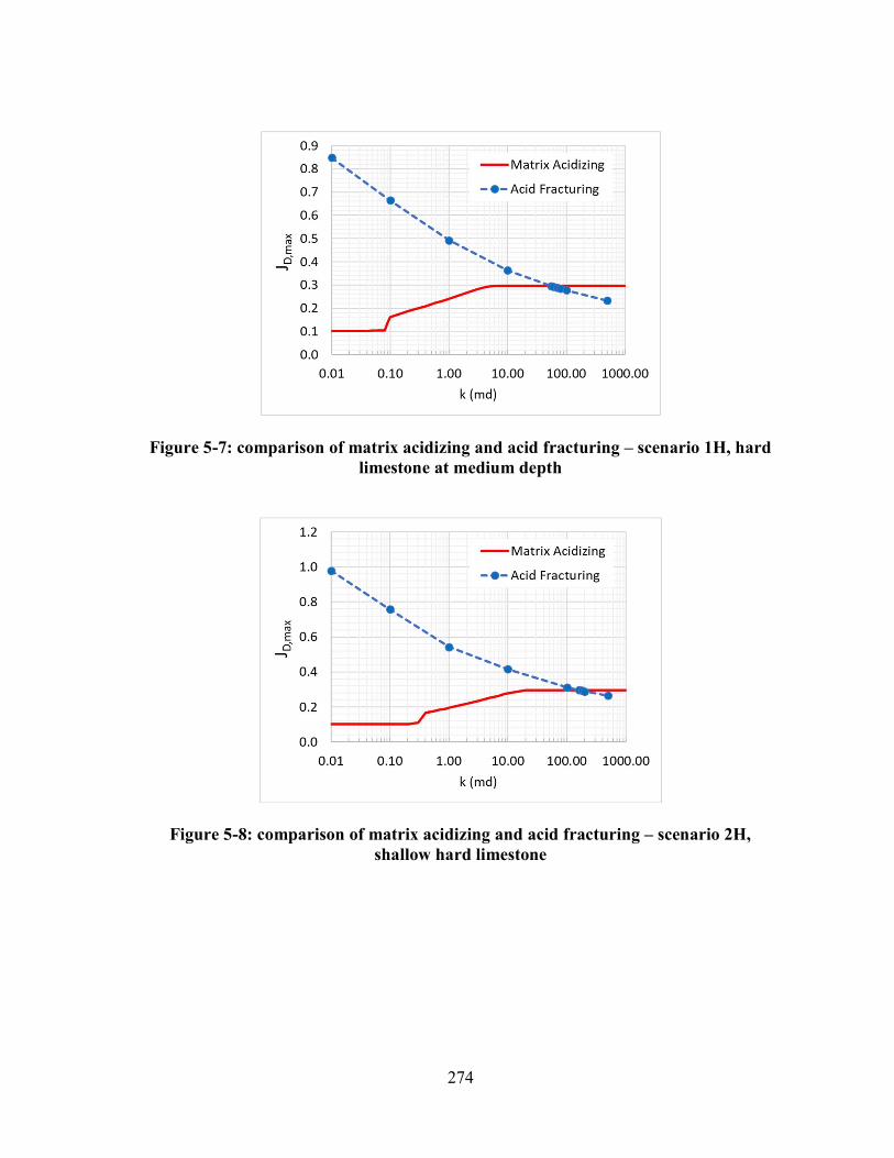
274

Figure 5-7: comparison of matrix acidizing and acid fracturing – scenario 1H, hard limestone at medium depth

Figure 5-8: comparison of matrix acidizing and acid fracturing – scenario 2H, shallow hard limestone

275

Figure 5-9: comparison of matrix acidizing and acid fracturing – scenario 3H, deep hard limestone

For scenario 1H (Figure 5-7), the cutoff permeability is 55 md. For scenario 2H

(Figure 5-8), it is 160 md. For scenario 3H (Figure 5-9), 15 md.

As expected, in all three scenarios, the hard rock results in a more productive acid

fracture when compared to the base cases. This results in a higher cutoff permeability,

when compared with the scenarios of softer rock. Comparing scenario 1H to 1, for

example, the cutoff permeability increased from 22 md to 55 md. Comparing scenario 2H

to 2 (shallow reservoir), it increased from 120 md to 160 md, and comparing 3H to 3 (deep

reservoir), it increased from around 2.5 md to 15 md.

The deeper the reservoir, the higher the impact of the rock embedment strength. In

the shallow reservoir, when 𝑆 increases from 50,000 psi to 200,000 psi, the cutoff

permeability increases 33%, from 120 to 160 md. In the deep reservoir, however, the

cutoff permeability goes from 2.5 md to 15 md, an increase of 600%. The reason for this

behavior is the confining stress, which is much higher in the deeper reservoir, requiring a

276

hard rock to withstand the fracture open. In the shallow reservoir, the confining stress is

small enough for the rock hardness to be less significant.

Figure 5-10 shows the comparison of different rock embedment strengths at the

same depths. The same plot presents the results for scenarios 1S, 1, and 1H, with rock

embedment strengths of 20,000 psi, 50,000 psi, and 200,000 psi, respectively. This plot

shows how the acid fracturing outcome varies with the rock embedment strength.

Figure 5-10: comparison of different rock embedment strengths

5.1.6. Scenarios 4 and 5 – different acid volumes

Scenarios 4 and 5 consist of the same reservoir as the base case (scenario 1), but

using different volumes of acid. While the base case used 500 bbl of 15% HCl, in scenario

277

4, that volume is reduced to 100 bbl (1 bbl/ft), and in scenario 5, it is increased to 2,000

bbl (20 bbl/ft).

The outcome of both stimulation methods for all three volumes of acid is presented

in Figure 5-11. As expected, the productivity index increases with the volume of acid for

both methods. Comparing Figure 5-11a with Figure 5-10 shows that for these scenarios

the volume of acid has a more significant impact on the acid fracturing outcome than the

rock embedment strength. The comparison between the methods for each volume of acid

is presented in Figure 5-12 (scenario 4) and Figure 5-13 (scenario 5).

Figure 5-11: impact of acid volume on (a) acid fracturing and (b) matrix acidizing

278

Figure 5-12: comparison of matrix acidizing and acid fracturing – scenario 4, 100bbl of acid

Figure 5-13: comparison of matrix acidizing and acid fracturing – scenario 5, 2,000bbl of acid

Although the larger acid volume results in higher productivity for both matrix

acidizing and acid fracturing, the results show that the impact on acid fracturing is more

pronounced, because the larger volumes of acid result in higher cutoff permeabilities. This

279

means that when more acid is employed, acid fracturing is the preferable technique over

a wider range of permeability. Comparing Figure 5-12, Figure 5-1, and Figure 5-13, it can

be seen that the cutoff permeability goes from 9 md (with 100 bbl of acid), to 22 md (with

500 bbl of acid), to 49 md (with 2,000 bbl of acid). This shows that the preferable

stimulation method is not only a function of the reservoir properties, but also of the volume

of acid that can be employed in the operation.

The same behavior is observed when analyzing rocks with other properties. For

example, performing the same analysis on the soft rock with embedment strength of

20,000 psi (scenario 1S), but other volumes of acid: 100 bbl (scenario 4S, Figure 5-14)

and 2,000 bbl (scenario 5S, Figure 5-15).

Figure 5-14: comparison of matrix acidizing and acid fracturing – scenario 4S, soft rock and 100 bbl of acid

280

Figure 5-15: comparison of matrix acidizing and acid fracturing – scenario 5S, soft rock and 2,000 bbl of acid

Comparing Figure 5-4, Figure 5-14, and Figure 5-15, the cutoff permeability goes

from 5 md (with 100 bbl of acid), to 12 md (with 500 bbl of acid), to 25 md (with 2,000

bbl of acid). Again, a larger volume of acid leads to acid fracturing being the preferable

method up to a higher permeability.

5.1.7. Scenario 6 – injector well

All scenarios presented so far considered a producer well, with bottomhole flowing

pressure gradient of 0.3 psi/ft. In an injector well, this bottomhole pressure gradient would

be higher, resulting in a smaller effective confining stress. Because of this, the acid fracture

conductivity is expected to be higher in an injector well than in a producer well. In scenario

6, the initial reservoir pore pressure gradient of 0.4333 psi/ft was used for calculating the

281

effective confining stress. All other properties are the same as the base case, scenario 1.

The results are presented in Figure 5-16.

Figure 5-16: comparison of matrix acidizing and acid fracturing – scenario 6, injector well

As expected, the injectivity index that can be obtained by acid fracturing the

injector well is higher than the corresponding productivity index of the producer well (for

this case, about 9% higher in average). The productivity of the matrix acidized well is the

same for injector and producer wells. This causes the acid fracturing technique to be

preferable up to a higher permeability for the injector well. For this scenario, the cutoff

permeability is 50 md for the injector well, compared to 22 md for the producer well.

282

5.1.8. Impact of the wormhole model

In all scenarios presented so far, the model used for wormhole propagation was the

new model proposed by this study (section 3.2 and Palharini Schwalbert et al., 2019c).

This has major implications in the predicted productivity of the matrix acidized well

performance, and consequently the cutoff permeability. The predicted acid fractured well

productivity is also affected because of the impact of the wormholes on acid leakoff. This

section analyzes the impact of different wormhole models.

Scenario 7 uses the model by Buijse and Glasbergen (2005), while scenario 8 uses

the model by Furui et al. (2010). The same values of 𝑃𝑉 , , and 𝑣 , , (in the

core scale) presented in Table 4-1 are used for all cases. Furui et al’s model requires the

additional parameters 𝑚 , 𝛼 , and 𝑑 , . The values used for these parameters in this

study are 𝑚 = 6, 𝛼 = 0.5, and 𝑑 , = 1 𝑚𝑚. All other parameters used in scenarios

7 and 8 are the same as used in scenario 1 (Table 4-1).

In scenario 7, the model by Buijse and Glasbergen (2005) was used to calculate

the wormhole propagation both for the matrix acidizing treatment and the acid fracturing

leakoff. However, Furui et al. (2010) did not present a version of their model for linear

flow, so it cannot be used to calculate wormhole propagation in the acid fracturing leakoff.

Because of that, in scenario 8, Furui’s model was used for the matrix acidizing

calculations, but for acid fracturing leakoff the volumetric model was used, with an

appropriate value of 𝑃𝑉 for each permeability, being the equivalent 𝑃𝑉 obtained by the

matrix acidizing simulation using Furui et al.’s model at that permeability.

283

Figure 5-17 shows the matrix acidized wells’ dimensionless productivity index

predicted using the three different models. Figure 5-18 shows the comparison between

matrix acidizing and acid fracturing using the model by Buijse and Glasbergen (2005),

and Figure 5-19 using the model by Furui et al. (2010).

Figure 5-17: impact of the wormhole model on matrix acidized well productivity

Figure 5-18: comparison of matrix acidizing and acid fracturing – scenario 7, Buijse and Glasbergen’s model

284

Figure 5-19: comparison of matrix acidizing and acid fracturing – scenario 8, Furui et al.’s model

As can be seen in Figure 5-17, the wormhole model has a major impact in the

matrix acidized well productivity, using the same core scale values of 𝑃𝑉 , , and

𝑣 , , . The model by Buijse and Glasbergen (2005) predicts a much smaller

productivity index because it applies no upscaling procedure on the values of 𝑃𝑉 , and

𝑣 , obtained in the core scale in laboratory experiments, as discussed in section 3.2.

Both the upscaled models (by Furui et al. and the new proposed model) predicted

higher productivity than Buijse and Glasbergen’s model, as expected. At high

permeability, both upscaled models have very similar predictions, with a difference of

only 2% above 40 md. In the medium permeabilty range, between 0.1 and 40 md, Furui’s

model predicted smaller productivity than the new model proposed in this study, because

it predicted a higher optimal injection rate that could only be achieved at higher

285

permeabilities. Furui’s model predicted that only face dissolution occurs up to 1 md, and

optimal conditions can only be achieved above 50 md, while the new model predicted face

dissolution only below 0.1 md, and optimal conditions achievable above 6 md.

Figure 5-18 shows that using the model by Buijse and Glasbergen (2005), acid

fracturing seems preferable for any permeability up to 480 md. Using Furui et al. (2010)’s

model, the cutoff permeability is 36 md (Figure 5-19). For comparison, using the new

proposed wormhole model results the cutoff permeability is 22 md (Figure 5-1). Both

upscaled models result similar cutoff permeabilities, while the not-upscaled model gives

a result one order of magnitude larger, contrary to field results.

These results illustrate the importance of the wormhole model in the prediction of

acid stimulation outcome in carbonates. For a good decision of the acid stimulation

method, accurate information regarding the wormhole model should be obtained, through

either laboratory experiments or history matching previous field treatments.

5.1.9. Scenario 9 – dolomite formation

All scenarios presented so far consisted of limestones composed of pure calcite.

Scenario 9 consists of a dolomite formation. The main difference between limestones and

dolomites concerning acid treatments is the reactivity of these minerals with the acid. The

reaction rate of dolomite with HCl is significantly lower than with limestone in usual

wellbore conditions. Table 4-2 shows the reaction kinetics constants for both minerals,

and 𝑘 is two orders of magnitude smaller for dolomite. While the reaction rate of calcite

286

with HCl can be regarded as infinite (mass transfer limited) for the temperatures of most

reservoirs, for dolomites the reaction kinetics is the limiting step unless the temperature is

high (around 300 ℉).

HCl has also a lower dissolving power for dolomite, so that the same volume of

acid can dissolve a smaller volume of mineral. The gravimetric dissolving power is 𝛽 =

1.27 mass of dolomite dissolved per unit mass of HCl (compared to 1.37 for calcite) and

the volumetric dissolving power is 𝜒 = 0.071 volume of dolomite dissolved per unit

volume of 15% HCl solution, compared to 0.082 for calcite.

Another implication of the lower reactivity and dissolving power of HCl with

dolomite is a smaller wormholing efficiency. The volume of acid required to create

wormholes in dolomite is larger than the corresponding volume for calcite, as reported by

Hoefner and Fogler (1988) and Wang et al. (1993). The data used in this study is that from

Ali and Nasr-El-Din (2018) for 15% HCl: 𝑃𝑉 , , = 3.3 and 𝑣 , , =

3.3 𝑐𝑚/𝑚𝑖𝑛, measured with cores of 1.5 in. by 6 in., with porosity around 15%.

Scenario 9 consists of a formation composed of pure dolomite, so that the

corresponding reaction kinetics, heat of reaction, dissolving power, and wormholing

parameters were used. All other parameters are the same as scenario 1 (Table 4-1).

The major difference between the two types of rocks is in the matrix acidizing

efficiency. Figure 5-20 shows the comparison of the best possible post-stimulation

dimensionless productivity index for limestone (scenario 1) and dolomite (scenario 9).

Figure 5-20a shows that the optimal outcome of acid fracturing does not change

significantly for the different rocks. However, as expected, Figure 5-20b shows that

287

matrix acidizing is more efficient in limestones, which have smaller 𝑃𝑉 values. Figure

5-21 shows the comparison between matrix acidizing and acid fracturing for the dolomite

scenario.

Figure 5-20: comparison of acid stimulation outcomes in limestone and dolomite

Figure 5-21: comparison of matrix acidizing and acid fracturing – scenario 9, dolomite

288

Because of the smaller wormholing efficiency in dolomites, acid fracturing is the

preferable stimulation technique over a larger range of permeability. Figure 5-21 shows a

cutoff permeability of 350 md for the dolomite rock, compared to 22 md for the limestone

of scenario 1 with the same geomechanical properties.

It is important to notice that, although the acid fracturing maximum productivity

in the dolomite case is not significantly different from the limestone (Figure 5-20a), the

operational conditions to obtain the maximum productivity are significantly different. In

general, the optimal injection rate is smaller for dolomites, especially for the higher

permeabilities (1 md and above). To illustrate this, Figure 5-22 shows the outcome of acid

fracturing for limestone (scenario 1) and dolomite (scenario 9).

Figure 5-22: optimal acid fracturing conditions for dolomite and limestone (1 md)

The maximum productivity achievable is similar for both rocks, but the optimal

injection rate is significantly different: 10 bpm for dolomite, and 100 bpm (maximum

289

value considered) for limestone. If 100 bpm is used to stimulate dolomite, the resulting

productivity is 40% smaller.

The reason for this behavior is the small reactivity of dolomite at low temperatures,

and the fact that the acid is heated as it is transported inside the fracture. This causes the

maximum reaction rate to happen at a position inside the fracture away from the wellbore.

Consequently, the etched width and conductivity profiles have a maximum away from the

wellbore, and the near-wellbore conductivity can be small. At the higher injection rates,

the acid is pushed far away from the wellbore before it has time to react, and the resulting

near-wellbore etched width and conductivity is too small.

Figure 5-23 presents the etched width and conductivity profiles for a 1 md

reservoir, for dolomite at the injection rates of 10 bpm (optimal) and 100 bpm, and for a

limestone reservoir with injection rate of 100 bpm (optimal injection rate for limestone).

Figure 5-23: (a) etched width and (b) conductivity profiles for dolomite and limestone

290

Notice that in the limestone case, the maximum etched width and conductivity is

located at the wellbore (origin). But in the dolomite cases there is a hump in the etched

width and conductivity profiles, illustrating that the maximum conductivity happens away

from the wellbore. In the dolomite case with injection rate of 100 bpm, the fracture is

longer than for 10 bpm, but too little rock is dissolved near the wellbore, resulting in too

small a conductivity near the wellbore. The result is a small productivity for the 100 bpm

case in dolomite. In fact, the etched width profile for the dolomite with 10 bpm injection

rate is more similar to the limestone optimal case, which occurs at 100 bpm injection rate.

As the limestone has a higher conductivity near the wellbore as well as a longer fracture

(compared to the dolomite case with 10 bpm), the productivity is higher for the limestone

case. The difference, however, is relatively small (Figure 5-20a): 𝐽 , = 0.419 for

dolomite with 10 bpm, and 𝐽 , = 0.433 for limestone with 100 bpm.

The maximum conductivity away from the wellbore in dolomites was previously

reported by Tinker (1991) and Al Jawad et al. (2018). This is a good example of the

importance of a fully-coupled acid fracturing simulator, that integrates the modeling of

fracture propagation, acid reaction, heat transfer, and productivity.

5.1.10. Summary of the Case Studies for Vertical Wells

Table 5-1 presents a summary of the case studies’ results. Acid fracturing is the

preferable method if the reservoir permeability is below 𝑘 , while matrix acidizing

is preferable above 𝑘 .

291

Table 5-1: Summary of Case Studies

Scenario Depth (ft) SRES (psi)

Vacid (bbl/ft)

Producer / Injector

Wormhole Model

Mineral 𝒌𝒄𝒖𝒕𝒐𝒇𝒇

(md)

1 10,000

50,000

5

Producer New model (this study, section 3.2)

Limestone

22

2 3,000 120

3 20,000 2.5

1S 10,000

20,000

12

2S 3,000 100

3S 20,000 1

1H 10,000

200,000

55

2H 3,000 160

3H 20,000 15

4

10,000

50,000 1 9

5 20 48

4S 20,000

1 5

5S 20 25

6

50,000 5

Injector 50

7

Producer

Buijse and Glasbergen

(2005) 480

8 Furui et al.

(2010) 36

9 New model (this study)

Dolomite 350

5.2. Concise Decision Criterion for Vertical Wells

In section 5.1, several case studies were presented to show which acid stimulation

method provides the greater productivity index for each scenario. A concise approximate

decision criterion is proposed in this section based on analytical equations.

292

In section 4.5, an analytical equation was proposed to estimate the maximum

productivity index that can be obtained with acid fracturing, equation (4.93). This

maximum acid fractured well dimensionless productivity index is denoted here by

𝐽 , , . Analogously, the maximum possible productivity index that can be achieved

with matrix acidizing, denoted here by 𝐽 , , , can be calculated using equation (3.83).

A reasonable decision criterion is to use acid fracturing when 𝐽 , , > 𝐽 , , , or,

in other words, when the productivity index ratio between acid fracture and matrix

acidizing is greater than one: , ,

, ,> 1. Using equations (4.93) and (3.83), the

productivity index ratio and decision criterion can be written as:

𝐽 , ,

𝐽 , ,=

ln

⎝

⎛ 𝑟

𝑟 +𝑉

𝜋𝜙ℎ𝑃𝑉 , ⎠

⎞ −34

ln

⎩⎪⎨

⎪⎧

𝑟𝜋

𝐶 , 𝑔(𝜆)+ 𝜁

𝐴𝐶 , 𝑘

𝜒𝑓 𝑉2(1 − 𝜙)ℎ ⎭

⎪⎬

⎪⎫

−34

> 1 (5.3)

The term 𝑃𝑉 , can be calculated by equation (3.39) if the injection rate during

the matrix acidizing treatment can be kept so that the acid interstitial velocity at the

wormhole front is always near the optimal value. To account for inefficiencies that cause

the value of 𝑃𝑉 in the field to be larger than the theoretical minimum, the term 𝑃𝑉 ,

can be substituted by 𝑃𝑉 , , which is an actual achievable value in the field under

293

consideration. Substituting 𝑃𝑉 , by 𝑃𝑉 , , after some algebra, the decision

criterion can be rewritten as:

𝐴𝐶 , 𝑘

𝜒𝑓 𝑉2(1 − 𝜙)ℎ

𝜋𝐶 , 𝑔(𝜆)

+ 𝜁 𝑟 +𝑉

𝜋𝜙ℎ𝑃𝑉 ,

> 1 (5.4)

The left-hand side of equation (5.4) is a dimensionless number that groups all

contributions from the reservoir, acid type and volume, wormholing efficiency, and acid

fracture conductivity. This dimensionless number is named here as “carbonate acid

stimulation number”, denoted by 𝑁 :

𝑁 =

𝐴𝐶 , 𝑘

𝜒𝑓 𝑉2(1 − 𝜙)ℎ

𝜋𝐶 , 𝑔(𝜆)

+ 𝜁 𝑟 +𝑉

𝜙𝜋ℎ𝑃𝑉 ,

(5.5)

The decision criterion is summarized as: if 𝑁 > 1, acid fracturing can result in

a higher productivity index than matrix acidizing; if 𝑁 < 1, matrix acidizing can result

in a higher productivity index.

The cut off permeability that divides the region of applicability of each technique,

𝑘 , can be calculated by equation (5.5), when 𝑁 = 1. It is given by:

294

𝑘 =

𝐴𝐶 ,

𝜒𝑓 𝑉2(1 − 𝜙)ℎ

𝜋𝐶 , 𝑔(𝜆)

+ 𝜁 𝑟 +𝑉

𝜙𝜋ℎ𝑃𝑉 ,

(5.6)

The terms 𝑔(𝜆) and 𝜁 come from the fracture productivity model by Meyer and

Jacot (2005), and can be calculated using equations (4.72) through (4.75). However, a

simplification can be done for square drainage areas, where 𝑔(𝜆) = 1, and 𝜁 can be

calculated by equation (4.95). Additionally, if the fracture is short compared to the

reservoir (𝐼 ≲ 0.2), which is usually the case when there is doubt between using acid

fracturing or matrix acidizing, then 𝐶 , = and 𝜁 = 2. In this case, the whole term

, ( )+ 𝜁 is simply equal to 4, which leads to the simplified equations:

𝑁 =

𝐴𝐶 , 𝑘

𝜒𝑓 𝑉2(1 − 𝜙)ℎ

4 𝑟 +𝑉

𝜙𝜋ℎ𝑃𝑉 ,

(5.7)

𝑘 =

𝐴𝐶 ,

𝜒𝑓 𝑉2(1 − 𝜙)ℎ

4 𝑟 +𝑉

𝜙𝜋ℎ𝑃𝑉 ,

(5.8)

295

In these equations, all the inefficiencies of the matrix acidizing and acid fracturing

operations are grouped in the terms 𝑓 and 𝑃𝑉 , . For the case studies presented in

section 5.1, in general 𝑃𝑉 , was high for low permeabilities at which it was not

possible to inject at optimal interstitial velocity, but 𝑃𝑉 , was close to 𝑃𝑉 ,

calculated by equation (3.39) once the permeability was high enough (plateau of matrix

acidizing curve in Figure 5-1 above 6 md, for example). As most of the intersection

between matrix acidizing and acid fracturing in section 5.1 happened on the plateau of the

matrix acidizing curve, for most cases presented, 𝑃𝑉 , ≈ 𝑃𝑉 , .

The fraction of acid spent etching, 𝑓 , depends on how much acid is lost due to

leakoff and to non-pay zones. It is a function of the leakoff coefficient and reservoir

properties, especially reservoir permeability. It depends strongly on the pressure

overbalance between the fracturing pressure and the reservoir pressure, 𝑝 − 𝑝 . Figure

4-27 shows one example of such dependence of 𝑓 on reservoir permeability, obtained

from the fully-coupled acid fracturing simulator. For that scenario, it seems that above 1

md 𝑓 decreases linearly proportional to the logarithm of the permeability. Based on all

the simulations presented in section 5.1, the following relation can be obtained:

𝑓 ≈ min 0.85 , 1.8615 − 0.069 × ln 𝑘 𝜎 , − 𝑝 (5.9)

where 𝑘 is the permeability in md, 𝜎 , is the minimum horizontal stress in psi, and 𝑝

is the initial reservoir pressure in psi. The function min(𝑎, 𝑏) results the minimum value

296

between 𝑎 and 𝑏. It was introduced because in the cases tested, 𝑓 was always below

0.85. The equation 1.8615 − 0.069 × ln 𝑘 𝜎 , − 𝑝 could result 𝑓 > 0.85

(which happens for 𝑘 𝜎 , − 𝑝 < 2.5 × 10 𝑚𝑑 𝑝𝑠𝑖 , or 𝑘 < 0.9𝑚𝑑 is the cases

presented in this study). In that case, it is better to assume 𝑓 = 0.85.

Equation (5.9) was obtained from the values of 𝑓 obtained in the simulations

presented in section 5.1. It is not general, and 𝑓 is expected to be different for different

reservoirs. In general, everything that causes a large acid leakoff tends to cause a smaller

𝑓 . When using loss control additives to reduce the acid loss, 𝑓 tends to be increased.

For the scenarios analyzed in section 5.1, however, equation (5.9) is a good

estimate of 𝑓 , and equations (5.7) and (5.8) can be used with this estimate of (5.9).

Figure 5-24 shows a comparison of the permeability cutoff obtained through the fully-

coupled simulations (section 5.1) and the quick estimate of equation (5.8). The black line

is the diagonal. The fact that most points are aligned with the diagonal shows how good

is the estimate of equation (5.8) and the proposed analytical decision criterion.

297

Figure 5-24: comparison of the permeability cutoff estimated with analytical equation and resulting from full simulations

There are 4 points that are not well aligned with the diagonal, and they correspond

to scenarios 3S, 7, 8, and 9. Scenarios 7, 8, and 9 are outliers from the general set because

they consisted respectively of Buijse and Glasbergen model, Furui model, and dolomite

formation, whereas all other cases were composed of limestone and used the wormhole

model proposed in this study. The error in scenarios 3S and 8 come from the fact that the

analytical estimate assumed 𝑃𝑉 , = 𝑃𝑉 , , but the cutoff permeability happens in

a permeability where the optimal interstitial velocity could not be reached. This can be

seen in Figure 5-6 and Figure 5-19, where the curve for acid fracturing intersects the curve

for matrix acidizing before the “plateau”. The error in scenarios 7 and 9 comes from the

fact that wormholing was much less efficient in these cases (Buijse and Glasbergen model

and dolomite), which caused leakoff to be smaller, hence the use of equation (5.9) to

298

estimate 𝑓 was not accurate. Still, even for these outliers, the correct order of magnitude

was predicted.

5.3. Concise Decision Criterion for Horizontal Wells

All comparisons presented so far considered vertical wells. For horizontal wells,

the comparison between matrix acidized or acid fractured wells is not so straightforward,

because the complexity and cost of completion is significantly different, because of stage

isolation. The fractured horizontal well usually has multiple fractures, so it involves more

variables, such as number of fractures, cluster and fracture spacing, etc. As for the matrix

acidized well, acid placement becomes a major concern, and a model that considers

diversion and flow inside the wellbore is necessary (such as presented by Furui et al.,

2012b).

Diversion is not the focus of this study, and in this section, for the sake of

simplicity and to obtain a concise decision criterion to select the preferable method for a

given volume of acid, it is assumed that the reservoir is homogeneous and a uniform acid

distribution is achieved. The well is assumed to be centered in the reservoir, and fully

penetrating. The frictional pressure drop along the horizontal wellbore is not considered.

While this may not be a good assumption for the cases of high permeability, it is good for

the comparison sought between the two stimulation techniques.

299

Different numbers of fractures are considered, but in all cases they are equally

spaced, and equal (all fractures are assumed to grow equally and receive the same volume

of acid). The volume of acid per foot of wellbore is the same in both matrix acidizing and

acid fracturing cases. In this sense, for a given volume of acid, in the cases with more

fractures, each fracture receives less acid. In the acid fractured wells, the production

contribution is assumed to come only from the fractures, which is equivalent to assuming

a plug-and-perf completion, where the wellbore is cased and cemented, and perforated

only at the fracture locations.

This comparison assumes pseudo-steady state, and the model by Babu and Odeh

(1989) is used for the matrix acidized well. For a centered fully penetrating well, the

dimensionless productivity index is given by:

𝐽 , =𝐿

ℎ𝐼 lnℎ 𝐼

𝑟+

𝜋6

𝑎ℎ𝐼

− 1.838 + 𝑠

(5.10)

where 𝑠 is the skin factor for the matrix acidized well, which in this case should be

calculated using the model by Furui et al. (2002):

𝑠 = − ln1

𝐼 + 1

𝑟

𝑟+

𝑟

𝑟+ 𝐼 − 1

(5.11)

300

For the acid fractured wells, as the fractures are equally spaced, each one drains

from their own drainage region, defined by the symmetry planes in between them. The

total productivity index of the horizontal well with multiple fractures is equal to the sum

of the productivity indices of each fracture. In general, the drainage area of each fracture

is not a square, but a rectangle. The more fractures are added, the more elongated is the

drainage area, which is represented by the aspect ratio 𝜆:

𝜆 =𝑎𝑁

𝐿

(5.12)

where 𝐿 is the wellbore length (equal to the reservoir length in the wellbore direction,

because the well is assumed to be fully penetrating), 𝑎 is the reservoir length in the fracture

direction (orthogonal to the wellbore), and 𝑁 is the number of fractures. Because the

drainage region of each fracture is far from square when the number of fractures is large,

the equations for square reservoirs cannot be used in this case (𝜁 and the shape factor 𝐶

must be calculated with the equations (4.74) through (4.76), and not the simplified

versions).

Because of the flow convergence towards the well, the “choke skin factor” 𝑠 must

be added, as presented by Mukherjee and Economides (1991):

𝑠 =𝑘 ℎ

𝑘 𝑤ln

ℎ

2𝑟−

𝜋

2=

ℎ

𝑥 𝐶ln

ℎ

2𝑟−

𝜋

2

(5.13)

301

The productivity of each fracture can be calculated by simulating the complete

operation using the fully-coupled acid fracturing simulator and adding the choke skin

factor 𝑠 , or it can be estimated by the analytical equations similar to those presented for

vertical wells in sections 4.5 and 5.2. As shown in those sections, although the fully-

coupled simulator is necessary to actually design the acid fracturing jobs, the analytical

estimate is satisfactory for the sake of comparing with matrix acidizing. For the horizontal

well with 𝑁 acid fractures, the optimal dimensionless productivity index can be estimated

by:

𝐽 , =2𝑁

ln

⎩⎪⎨

⎪⎧

4𝑎𝐿𝜋

𝐶 , 𝑔(𝜆)+ 𝜁 (𝜆, 𝐼 ) 𝑒

𝑁 𝑒 𝐶 (𝜆)𝐴

𝐶 , 𝑘𝜒𝑓 𝑉

2(1 − 𝜙)ℎ𝑁 ⎭⎪⎬

⎪⎫

(5.14)

where 𝑒 is the exponential of Euler’s constant (𝑒 ≈ 1.781), 𝜁 (𝜆, 𝐼 ) is a function of

the aspect ratio 𝜆 and the fracture penetration ratio 𝐼 (in this case defined as 𝐼 = 2𝑥 /𝑎),

calculated by equation (4.74), and 𝐶 (𝜆) is also a function of 𝜆 and can be calculated by

equation (4.79).

The dependence of the productivity index on the number of fractures is not

straightforward, because 𝑁 appears several times in equation (5.14), and 𝜆 is proportional

to 𝑁 . For a given volume of acid injected at the whole well, as the number of fractures

increases, the amount of acid that each fracture receives diminishes. For a given scenario,

302

there is an optimal number of fractures that results in the maximum productivity for the

whole multi-fractured well.

The ratio of the productivity indices of the acid fractured to the matrix acidized

well can be calculated by dividing equation (5.14) by (5.10). This ratio is denoted here by

𝑃𝐼𝑅 (productivity index ratio), and it is given by:

𝑃𝐼𝑅 =𝐽 ,

𝐽 ,=

2𝑁 ℎ𝐼𝐿

lnℎ 𝐼

𝑟+

𝜋6

𝑎ℎ𝐼

− 1.838 + 𝑠

ln

⎩⎪⎨

⎪⎧

4𝑎𝐿𝜋

𝐶 , 𝑔(𝜆)+ 𝜁 (𝜆, 𝐼 ) 𝑒

𝑁 𝑒 𝐶 (𝜆)𝐴

𝐶 , 𝑘𝜒𝑓 𝑉

2(1 − 𝜙)ℎ𝑁 ⎭⎪⎬

⎪⎫

(5.15)

The decision criterion for the preferable acid stimulation method for horizontal

wells can be summarized as: if 𝑃𝐼𝑅 > 1, the well with multiple acid fractures has higher

productivity than the matrix acidized horizontal well; if 𝑃𝐼𝑅 < 1, the matrix acidized well

produces more.

The cutoff permeability for the horizontal well can be isolated from equation (5.15)

by making 𝑃𝐼𝑅 = 1, resulting:

303

𝑘 , =𝐴

𝐶 ,

𝜒𝑓 𝑉

2(1 − 𝜙)ℎ𝑁

×

⎩⎪⎨

⎪⎧

𝑒.

4𝑎𝐿𝑒𝑁 𝑒 𝐶 (𝜆)

𝜋𝐶 , 𝑔(𝜆)

+ 𝜁 (𝜆, 𝐼 )⎭⎪⎬

⎪⎫

(5.16)

Some examples are presented in the following.

5.3.1. Scenario 10 – horizontal well

The scenario analyzed here is based on the base case (scenario 1, Table 4-1), but

the drainage region of the well is a square of 5,000 ft x 5,000 ft, and instead of a vertical

well there is a fully penetrating horizontal well. The volume of acid is 1 bbl/ft.

Figure 5-25 shows the dimensionless productivity index of the matrix acidized

horizontal well, for permeabilities ranging from 0.01 md to 1000 md. The productivity

index is smaller at very low permeabilities, because it is not possible to inject at optimal

injection rate for wormhole propagation. However, the impact of the skin factor in

horizontal wells is much smaller, so the difference between minimum and maximum

achievable 𝐽 , is not so large. Basically, for this case, 𝐽 , ranges from 1.3 to 1.9.

304

Figure 5-25: dimensionless productivity index of the matrix acidized horizontal well

The productivity index of the acid fractured well depends significantly on the

number of fractures. Figure 5-26 shows the dimensionless productivity index of the acid

fractured horizontal well, 𝐽 , , for different numbers of transverse acid fractures. As can

be seen, there is an optimal number of fractures for a given scenario. In this case, analyzing

the lowest permeability plotted, 0.01 md, Figure 5-26 shows that the maximum 𝐽 , is

achieved with 4 fractures. For this scenario, if there are more than 4 fractures, each one

receives too little acid and is not conductive enough, as shown by the curves with 5 and

10 fractures in Figure 5-26. As will be shown later, a larger volume of acid changes this

picture, allowing to effectively make more fractures.

305

Figure 5-26: dimensionless productivity index of the horizontal well with multiple acid fractures

To compare both stimulation methods, Figure 5-27 shows the ratio of the

productivity indices of the acid fractured to the matrix acidized well. As observed for the

vertical wells, there is a value of permeability above which matrix acidizing results in

higher productivity than acid fracturing.

306

Figure 5-27: comparison of matrix acidized and acid fractured horizontal well – scenario 10

In this scenario, if the permeability is above 0.6 md, there is no number of fractures

that can make the acid fractured well more productive than the matrix acidized well

Although only the curves for 1, 4, and 100 fractures are shown, the productivity for all

other numbers of fractures is in between these. At low permeabilities, if the right number

of fractures is used, acid fracturing can be much more productive than matrix acidizing.

In this case, if the reservoir permeability is 0.01 md, the acid fractured well with 4 fractures

has a productivity 7 times higher than the matrix acidized well.

The shape of the drainage area also has an impact. In scenario 10, a square drainage

area 5,000 ft by 5,000 ft was considered. If the well spacing is reduced to 2,000 ft, resulting

in a rectangular drainage area 2,000 ft by 5,000 ft, still with a fully penetrating 5,000 ft

long horizontal well, two things change: (1) the productivity index of the horizontal well

307

itself becomes higher and the impact of matrix acidizing increases (the value of 𝑎 in

equation (5.10) is smaller), and (2) a larger number of fractures becomes optimal at small

permeabilities. Figure 5-28 shows the results for this rectangular drainage area.

(a) matrix acidized well (b) productivity index ratio

Figure 5-28: comparison between matrix acidizing and acid fracturing for 2,000 ft by 5,000 ft drainage area; (a) matrix acidized well, (b) PI ratio.

Figure 5-28a shows the dimensionless productivity index of the matrix acidized

well. The maximum is 4.7 for the rectangular drainage area, much greater than the 1.9

obtained for the square drainage area. Figure 5-28b shows the productivity index ratio

between matrix acidizing and acid fracturing. In this case, the cutoff permeability did not

change, being around 0.6 md for both square and rectangular drainage areas. If the

permeability is above 0.6 md, there is no number of fractures that can make an acid

fractured well more productive than the matrix acidized well. But in reservoir

permeabilities below 0.6 md, the acid fractured well is much more productive, and in this

case the optimal number of fractures for the reservoir of 0.01 md is 10 fractures (compared

308

to 4 fractures in the square drainage area). Because the fractures do not have to be so long

to drain the rectangular area, there is enough acid to effectively stimulate a larger number

of fractures.

5.3.2. Scenario 11 – larger acid volume

This scenario compares what happens when the acid volume is increased to the

extremely high value of 10 bbl/ft (compared to 1 bbl/ft used in scenario 10). The square

drainage area of 5,000 ft by 5,000 ft is used for the comparison. Figure 5-29 shows the

dimensionless productivity index of the matrix acidized horizontal well. Figure 5-30

shows the same for the acid fractured horizontal well, with different numbers of transverse

fractures.

Figure 5-29: dimensionless productivity index of the matrix acidized horizontal well

309

Figure 5-30: dimensionless productivity index of the horizontal well with multiple acid fractures

The outcome for the matrix acidized well is not too different than what was

obtained with 1 bbl/ft of acid (Figure 5-25). This happens because the productivity of a

horizontal well is less sensitive to the skin factor. The major difference occurs in the low

permeabilities, in which 𝐽 , increased from 1.3 (using 1 bbl of acid per foot) to 1.74

(using 10 bbl of acid per foot). The reason is that 1 bbl/ft was not enough to bypass the

damage region in the low permeabilities, while 10 bbl/ft is (even at low injection rates).

For the high permeabilities, however, where it is possible to inject at optimal injection

rate, 𝐽 , goes from 1.7 (using 1 bbl of acid per foot) to 1.98 (using 10 bbl/ft).

On the other hand, the outcome of the acid fracturing treatment is significantly

improved by the higher acid volume, especially at the lower permeabilities. Figure 5-30

310

shows that the optimal number of fractures is larger, being equal to 10 fractures for the

permeability of 0.01 md (compared to 4 fractures in the case with smaller acid volume).

Figure 5-31 shows the ratio of the productivity index of the acid fractured to the

matrix acidized well. Figure 5-31a shows the full range of permeabilities, and Figure

5-31b shows a detail of the intersection. At a permeability of 0.01 md, the acid fractured

well with 10 transverse fractures produces more than 70 times more than the matrix

acidized well. Still, if the permeability is high enough, the matrix acidized well is more

productive. In this case, the acid fractured well can be more productive up to near 50 md,

but above 50 md there is no number of fractures that results in a more productive well

than matrix acidizing.

Figure 5-31: comparison of matrix acidized and acid fractured horizontal well – scenario 11; (a) full range of permeability, (b) detail of the intersection If this massive volume of acid of 10 bbl/ft is used in the 2,000 ft by 5,000 ft

rectangular drainage region, the result is analogous to that observed in scenario 10: a larger

311

number of fractures becomes preferable in the lower permeabilities, and the cutoff

permeability does not change significantly. Figure 5-32 shows the productivity index ratio

between matrix acidized and acid fractured well for the rectangular drainage region with

the massive acid volume. As can be seen, at the permeability of 0.01 md, the optimal

number of fractures becomes 28 (compared to 10 for the square drainage region). The

cutoff permeability does not change significantly, being slightly smaller than 50 md.

Figure 5-32: PI ratio between matrix acidizing and acid fracturing for rectangular 2,000 ft by 5,000 ft drainage area with massive acid volume.

5.3.3. Soft chalks

The North Sea soft chalks consist of a typical example of field case where the

industry has been matrix acidizing wells in low permeabilities, on the order of 1 md (Furui

312

et al., 2012, and Burton et al., 2018). These chalks have high porosity, around 35%, and

are efficiently wormholed, often resulting skin factors smaller than -4 and mean values of

𝑃𝑉 , smaller than 0.03 (see Furui et al., 2012, Burton et al., 2018, and in this study,

section 3.2.4.2).

Additionally, they are usually soft rocks. Melendez et al. (2007) measured the rock

embedment strength of North Sea soft chalks and presented an average value of 𝑆 =

3,107 𝑝𝑠𝑖. Velasquez (2017) conducted acid fracture conductivity experiments with these

chalks, and although she did not report values of 𝑆 , the fracture conductivity obtained

was very low, characteristic of extremely soft rocks.

However, not all North Sea chalks are the same. Cook and Brekke (2004)

presented a classification of the different fields, showing that while some chalks are indeed

soft, others are harder. Vos et al. (2007) studied 4 different assets, with estimated values

of 𝑆 between 20,000 and 80,000 psi, and reported values of Young’s modulus between

0.7x106 and 2.2x106 psi. Vos et al. (2007) also reported effective confining stresses

varying from 1,500 psi to more than 7,000 psi.

With these values, it is possible to determine which is the best acid stimulation

method. Three scenarios are considered here: extremely soft chalk (scenario 12), medium

chalk (scenario 13), and “hard” chalk (scenario 14). The values of the rock embedment

strength and other parameters used are presented in Table 5-2, based on the references

cited above. The acid volume used is the median value presented by Burton et al. (2018)

after the analysis of more than 600 acid jobs: 1.79 bbl/ft of 28% HCl. Cook and Brekke

(2004) mention depths between 7,800 and 10,200 ft, so a representative value of 9,000 ft

313

is used in this study. The drainage region of the well is assumed to measure 5,000 ft x

5,000 ft, with a centered fully penetrating horizontal well. The parameters for the

wormhole propagation model are those representative of the field case published by Furui

et al. (2010), presented in section 3.2.4.2. Other parameters not presented here are the

same presented in Table 4-1.

Table 5-2: parameters used for the soft chalks of scenarios 12, 13, and 14

Parameter Scenario 12 Scenario 13 Scenario 14 Rock embedment strength 3,107 psi 20,000 psi 80,000 psi

Porosity 40% 35% 30% Acid concentration 28% HCl 28% HCl 28% HCl

Acid volume 1.79 bbl/ft 1.79 bbl/ft 1.79 bbl/ft Depth 9,000 ft 9,000 ft 9,000 ft

Effective Confining Stress 4,000 psi 4,000 psi 4,000 psi

The productivity index ratios between acid fracturing and matrix acidizing for

these scenarios are plotted in Figure 5-33, Figure 5-34, and Figure 5-35, for scenarios 12,

13, and 14 respectively.

314

Figure 5-33: comparison of matrix acidized and acid fractured horizontal well – scenario 12, extremely soft chalk

Figure 5-34: comparison of matrix acidized and acid fractured horizontal well – scenario 13, medium chalk

315

Figure 5-35: comparison of matrix acidized and acid fractured horizontal well – scenario 14, “hard” chalk

As can be seen from Figure 5-33, matrix acidizing is more productive than acid

fracturing in all cases tested for the soft chalk with only 3107 psi of rock embedment

strength. The rock is so soft that no number of fractures can make a more productive well

than the matrix acidized well for the range of permeabilities plotted, above 0.1 md. This

agrees with the industry practice presented by Furui et al. (2010) and Burton et al. (2018),

which includes several wells with permeabilities around 0.2 md, successfully matrix

acidized. For rocks as soft as this scenario, if matrix acidizing does not yield enough

productivity, hydraulic fracturing with proppant is necessary, with special concern about

proppant embedment.

Figure 5-34 and Figure 5-35 show that, if the chalk is not so soft as scenario 12,

acid fracturing may become a better alternative if the permeability is small enough. The

rock embedment strength in scenario 13 is 20,000 psi, and Figure 5-34 shows that acid

316

fracturing is preferable if the reservoir permeability is below 3 md, with the optimal

number of fractures being 5. Figure 5-35 shows that for scenario 14, with rock embedment

strength of 80,000 psi, acid fracturing is preferable if the reservoir permeability is below

9 md. The optimal number of fractures is also 5.

317

6. CONCLUSIONS

In this dissertation, a few different topics regarding acid stimulation in carbonate

reservoirs were studied. The main conclusions for each topic are presented in the

following.

The main conclusions regarding modeling of matrix acidizing in carbonates are:

The Two-Scale Continuum Model can be used to represent real matrix acidizing

behavior, if adequately tuned. The computation cost and amount of input required,

however, makes it impractical for simulating field treatments. The value of the

Two-Scale Continuum Model lies more on aiding the understanding of how the

wormholing phenomenon behaves at small scales for different conditions and

geometries.

In anisotropic carbonates, the wormholes formed may be aligned with the direction

of higher permeability. This behavior was observed in the simulations using the

Two-Scale Continuum Model and also in experiments. It was observed, however,

that this may not occur if the injection rate is small, even in anisotropic formations.

In this sense, in a reservoir where the horizontal permeability is much greater than

the vertical permeability, if the injection rate is high enough, the wormhole

network is expected to propagate more in the horizontal direction than in the

vertical. The wormhole network that arises from an openhole horizontal well is

expected to be elliptical, and not cylindrical as would be expected for isotropic

formations. When using a limited entry completion, the wormhole network that

318

arises from each acid injection point is expected to be ellipsoidal if the formation

is anisotropic (opposed to the spherical shape expected from isotropic formations).

These different shapes of the wormhole networks in anisotropic formations impact

the skin factor and productivity resulting from matrix acidizing these formations.

New equations to calculate the skin factor in these scenarios were derived and

presented in this study.

When using limited entry completions to matrix acidize a well, there is an optimal

stimulation coverage: 2/3. If the stimulation coverage is smaller than 60%, the

partial completion effect is significant, impairing the productivity.

Although the limited entry completion can significantly improve acid placement,

it does not have a great impact on the skin factor itself, if it is possible to inject at

optimal injection rate without limited entry. For stimulation coverages from 60%

to 100% (which corresponds to a fully completed / fully stimulated well), there is

no significant difference in productivity.

A new upscaled global model of wormhole propagation was presented, based on

experimental results and large scale simulations using the Two-Scale Continuum

Model. The new proposed global model accounts for the different wormhole

propagation that occurs at different scales, and can satisfactorily represent core

flooding experiments (small scale), large blocks experiments (intermediate scale),

and field treatments (large scale). It is a correlation simple enough to be used as a

practical engineering tool for field treatment design.

319

The main conclusions regarding the modeling of acid fracturing are:

The acid leakoff can be significantly increased by wormhole propagation from the

fracture faces, but only in formations where wormhole propagation is efficient. A

new acid leakoff model was proposed taking this into account, equations (4.21)

through (4.28), algorithm in Figure 4-3. In cases of efficient wormholing, this

model predicts leakoff coefficients even larger than the formation fluids

compression coefficient, 𝐶 .

Based on the proposed acid leakoff model, a dimensionless number that controls

the impact of wormholes on leakoff was proposed. In this work, this dimensionless

number was called the “number of leakoff with wormholes”, and denoted by

𝑁 =, , √

. The larger the number 𝑁 , the more significant is the

effect of wormholes on leakoff. If the value of 𝑁 is very small (say,

𝑁 ~0.01), the wormholes’ impact on leakoff is negligible. A value 𝑁 ≳ 0.4

can be considered large, in which the leakoff coefficient can be significantly larger

than 𝐶 , and increase with time due to wormhole propagation.

It is possible to optimize the design of acid fracturing operations using the fully-

coupled acid fracturing model presented by Al Jawad et al. (2018), integrated with

the productivity model presented in this dissertation (section 4.3). It is possible to

determine, for a given scenario, which type of fluid, injection rate, and amount of

pad should be used to obtain the maximum possible productivity of the acid

fractured well.

320

The optimal operational parameters for acid fracturing depend on the reservoir

properties, and a fully-coupled simulator is necessary for the optimization. As a

general rule, for cases where long acid fractures are sought (low permeabilities),

more retarded acid systems are required, while when the acid fracture does not

have to be so long (high permeabilities) straight acid can be used. For the example

cases presented, it was observed that for a permeability of 0.01 md emulsified acid

is generally a good option, while for a permeability of 0.1 md gelled acid is

recommended, and above 1 md, in general, straight acid should be used. Due to

the slower reactivity, the optimal injection rate for dolomites is, in general, much

smaller than that for limestones and chalks.

Analytical equations were presented to estimate the theoretical maximum

dimensionless productivity index that can be achieved with acid fracturing, using

a given volume of acid: equations (4.82) or (4.93) for vertical wells, and equation

(5.14) for horizontal wells with multiple fractures. It must be pointed out that the

theoretical optimal productivity estimated with the proposed analytical equations

may not be physically achievable due to practical limitations, especially in cases

where the theoretical optimal fracture length is too long (live acid may not reach

that length), or the permeability is too large (leakoff may make acid fracturing

impractical). For the cases tested, however, the prediction of the analytical

equations is close to the results of the fully-coupled acid fracturing simulator.

The simulations indicate that for the cases analyzed it is possible to obtain a

fractured well productivity index close to the theoretical maximum, if the acid lost

321

by leakoff is discounted and the right operational parameters are used (acid system,

injection rate, etc). The optimal operational parameters, however, are different for

each scenario, and a fully-coupled simulator should be used to determine them

when designing an acid fracturing treatment.

The main conclusions regarding the comparison between acid fracturing and

matrix acidizing are:

Acid fracturing results in a higher productivity index at lower permeabilities, while

matrix acidizing requires a minimum permeability that allows injecting the acid

near the optimal injection rate for wormhole propagation. For each scenario, there

is a value of permeability above which matrix acidizing can result in a more

productive well than acid fracturing, using the same volume of acid. In this

dissertation, this permeability is called cutoff permeability, 𝑘 .

The value of the cutoff permeability depends on several reservoir properties, such

as the rock mechanical properties, mineralogy, horizontal stress, other parameters

that determine the acid fracture conductivity, acid wormholing efficiency

parameters such as 𝑃𝑉 , and 𝑣 , , acid type, concentration, and volume, and

reservoir pressure.

General values of the cutoff permeability were presented for several case studies.

Everything that makes the acid fracture more conductive contributes to increase

the cutoff permeability (meaning that acid fracturing is the preferred technique for

a larger range of permeabilities). For example, harder rocks and shallower

322

reservoirs have higher cutoff permeability than softer rocks and deeper reservoirs.

Analogously, everything that improves the efficiency of matrix acidizing

treatments contributes to decreasing the cutoff permeability. For example,

dolomites have greater values of 𝑃𝑉 , than limestones, and so dolomites tend

to have higher cutoff permeability. In general, the cutoff permeability tends to be

smaller for horizontal wells than for vertical wells.

In horizontal wells with multiple acid fractures, there is an optimal number of

fractures for a given scenario. As the volume of acid is fixed in the analysis, if too

many acid fractures are made, each one does not receive enough acid, having

insufficient conductivity. The optimal number of acid fractures increases with the

acid volume, and decreases with the well spacing.

Concise analytical decision criteria for the best acid stimulation method were

proposed for both vertical wells and horizontal wells with multiple acid fractures.

The decision criterion for vertical wells is presented by equation (5.4), and for

horizontal wells by equation (5.15). The cutoff permeability for a vertical well can

be estimated by equation (5.6), and for a horizontal well by equation (5.16).

323

REFERENCES

Akanni, O. O., & Nasr-El-Din, H. A. (2015, March 8). The Accuracy of Carbonate Matrix-Acidizing Models in Predicting Optimum Injection and Wormhole Propagation Rates. Society of Petroleum Engineers. doi:10.2118/172575-MS.

Akanni, O. O., & Nasr-El-Din, H. A. (2016, September 26). Modeling of Wormhole Propagation During Matrix Acidizing of Carbonate Reservoirs by Organic Acids and Chelating Agents. Society of Petroleum Engineers. doi:10.2118/181348-MS

Al Jawad, M. S. (2018). Development of a Fully Integrated Acid Fracture Model. PhD Dissertation, Texas A&M University, College Station, TX.

Aldhayee, K., Ali, M. T., & Nasr-El-Din, H. A. (2018, October 16). Acid Wormholing in Multistage Acid Fractured Wells Completed in Tight Naturally Fractured Dolomite Formation: Benefits and Impacts on Acid Fracturing Stimulation Design. Society of Petroleum Engineers. doi:10.2118/191440-18IHFT-MS

Al-Duailej, Y. K., Kwak, H. T., Caliskan, S., & Al-Yami, I. S. (2013, March 26). Wormhole Characterisation Using NMR. International Petroleum Technology Conference. doi:10.2523/IPTC-17063-MS.

Ali, M. T., & Nasr-El-Din, H. A. (2018, June 1). A Robust Model To Simulate Dolomite-Matrix Acidizing. Society of Petroleum Engineers. doi:10.2118/191136-PA

Aljawad, M. S., Zhu, D., and Hill, A. D. 2016. Modeling Study of Acid Fracture Fluid System Performance. Paper SPE 179109 presented at the SPE Hydraulic Fracturing Technology Conference, The Woodlands, Texas, 9-11 February.

Aljawad, M. S., Zhu, D., & Hill, A. D. (2018a, June 8). Temperature and Geometry Effects on the Fracture Surfaces Dissolution Patterns in Acid Fracturing. Society of Petroleum Engineers. doi:10.2118/190819-MS

Aljawad, M. S., Schwalbert, M. P., Zhu, D., & Hill, A. D. (2018b, October 16). Guidelines for Optimizing Acid Fracture Design Using an Integrated Acid Fracture and Productivity Model. Society of Petroleum Engineers. doi:10.2118/191423-18IHFT-MS

Azevedo, C. T., Rosolen, M. A., Rocha, J. D. H., Neumann, L. F., & Melo, R. C. L. (2010, January 1). Challenges Faced to Execute Hydraulic Fracturing In Brazilian Pre-Salt Wells. American Rock Mechanics Association.

324

Babu, D. K., & Odeh, A. S. (1989, November 1). Productivity of a Horizontal Well (includes associated papers 20306, 20307, 20394, 20403, 20799, 21307, 21610, 21611, 21623, 21624, 25295, 25408, 26262, 26281, 31025, and 31035). Society of Petroleum Engineers. doi:10.2118/18298-PA

Bagrintseva, K. I., 2015. Carbonate Reservoir Rocks. John-Wiley & Sons.

Ben-Naceur, K., & Economides, M. J. (1989, January 1). Design and Evaluation of Acid Fracturing Treatments. Society of Petroleum Engineers. doi:10.2118/18978-MS

Berman, A.S. 1953. Laminar Flow in Channels with Porous Walls. J. Appl. Phys. 24(9): 1232-1235.

Buijse, M. A. (2000, August 1). Understanding Wormholing Mechanisms Can Improve Acid Treatments in Carbonate Formations. Society of Petroleum Engineers. doi:10.2118/65068-PA.

Buijse, M. A., & Glasbergen, G. (2005, January 1). A Semi-Empirical Model To Calculate Wormhole Growth in Carbonate Acidizing. Society of Petroleum Engineers. doi:10.2118/96892-MS.

Burton, R. C., Nozaki, M., Zwarich, N. R., & Furui, K. (2018, September 17). Improved Understanding of Acid Wormholing in Carbonate Reservoirs Through Laboratory Experiments and Field Measurements. Society of Petroleum Engineers. doi:10.2118/191625-MS.

Carter, R.D.: “Derivation of the General Equation for Estimating the Extent of the Fractured Area,” Appendix I of “Optimum Fluid Characteristics for Fracture Extension,” Drilling and Production Practice, G.C. Howard and C.R. Fast, New York, New York, USA, American Petroleum Institute (1957), 261–269.

Cash, R., Zhu, D., & Hill, A. D. (2016, August 24). Acid Fracturing Carbonate-Rich Shale: A Feasibility Investigation of Eagle Ford Formation. Society of Petroleum Engineers. doi:10.2118/181805-MS.

CFD Direct. 2016. http://cfd.direct (accessed 8 December 2016).

Chang, F. F. and Fogler, H. S.: “Carbonate Acidizing”. Chapter 4 in “Acid Stimulation”, Monograph Volume 26 from Society of Petroleum Engineers, organized by Ali, S. A., Kalfayan, L. J., and Montgomery, C. T., 2016.

325

Cheng, H., Schwalbert, M. P., Hill, A. D., & Zhu, D. (2019, March 22). A Fundamental Model for Wormhole Formation Including Multiphase Flow. International Petroleum Technology Conference. doi:10.2523/19121-MS

Cinco-Ley, H. and Samaniego, F.: “Transient Pressure Analysis for Fractured Wells”, JPT 1749-4766, September 1981.

Cleary, M. P. 1980. Comprehensive Design Formulae for Hydraulic Fracturing. Paper SPE 9259 presented at the Annual Technical Conference and Exhibition, Dallas, Texas, 21-24 September.

Cleary, M. P., Kavvadas, M., and Lam, K. Y. 1983. Development of a Fully Three-Dimensional Simulator for Analysis and Design of Hydraulic Fracturing. Paper SPE/DOE 11631 presented at the Low Permeability Gas Reservoirs Symposium, Denver, Colorado, 14-16 March.

Cohen, C.E., Ding, D., Quintard, M., and Bazin, B., 2008. From Pore Scale To Wellbore Scale: Impact Of Geometry On Wormhole Growth In Carbonate Acidization. Chemical Engineering Science. 63 (12):3088-3099. DOI: 10.1016/j.ces.2008.03.021.

Cook, C. C., & Brekke, K. (2004, April 1). Productivity Preservation Through Hydraulic Propped Fractures in the Eldfisk North Sea Chalk Field. Society of Petroleum Engineers. doi:10.2118/88031-PA

Crowe, C. W., Hutchinson, B. H., & Trittipo, B. L. (1989, May 1). Fluid-Loss Control: The Key to Successful Acid Fracturing. Society of Petroleum Engineers. doi:10.2118/16883-PA

Daccord, G., & Lenormand, R. (1987). Fractal patterns from chemical dissolution. Nature, 325. doi: 10.1038/325041a0.

Daccord, G., Touboul, E., & Lenormand, R. (1989, February 1). Carbonate Acidizing: Toward a Quantitative Model of the Wormholing Phenomenon. Society of Petroleum Engineers. doi:10.2118/16887-PA.

Daneshy, A., Valkó, P., and Norman, L.: “Well Stimulation”. Chapter 17 in: “Petroleum Well Construction”, Edited by M. J. Economides, L. T. Watters, and S. Dunn-Norman, Wiley, Chichester, New York, 1998.

De Oliveira, T. J. L., De Melo, A. R., Oliveira, J. A. A., & Pereira, A. Z. I. (2012, January 1). Numerical Simulation of the Acidizing Process and PVBT Extraction Methodology Including Porosity/Permeability and Mineralogy Heterogeneity. Society of Petroleum Engineers. doi:10.2118/151823-MS.

326

Deng, J. (2010). Mechanical Behavior of Small-Scale Channels in Acid-Etched Fractures. PhD Dissertation, Texas A&M University, College Station, TX.

Deng, J., Mou, J., Hill, A.D., and Zhu, D. 2012. A New Correlation of Acid-Fracture Conductivity Subject to Closure Stress. SPE Prod. & Oper. 27(2): 158-169.

Dietz, D. N. (1965, August 1). Determination of Average Reservoir Pressure From Build-Up Surveys. Society of Petroleum Engineers. doi:10.2118/1156-PA

Doerler, N. and Prouvost, L. P.: “Diverting Agents: Laboratory Study and Modeling of Resultant Zone Injectivities”, SPE 16250, 1987.

Dong, K., Jin, X., Zhu, D., & Hill, A. D. (2014, February 26). The Effect of Core Dimensions on the Optimal Acid Flux in Carbonate Acidizing. Society of Petroleum Engineers. doi:10.2118/168146-MS.

Dong, K., Zhu, D., & Hill, A. D. (2017, June 1). Theoretical and Experimental Study on Optimal Injection Rates in Carbonate Acidizing. Society of Petroleum Engineers. doi:10.2118/178961-PA.

Earlougher, R. C., Ramey, H. J., Miller, F. G., & Mueller, T. D. (1968, February 1). Pressure Distributions in Rectangular Reservoirs. Society of Petroleum Engineers. doi:10.2118/1956-PA

Economides, M. J. and Martin, T.: “Modern Fracturing – Enhancing Natural Gas Production”, Gulf Publishing, Houston, TX, 2007.

Economides, M. J., and Nolte, K. G.: “Reservoir Stimulation”, 3 Ed., London, UK, John Wiley & Sons, 2000.

Economides, M. J., Hill, A. D., Ehlig-Economides, C. E.: “Petroleum Production Systems”. Prentice Hall, Upper Saddle River, NJ, 1994.

Economides, M. J., Hill, A. D., Ehlig-Economides, C., and Zhu, D. 2013. Petroleum Production Systems, second edition. Upper Saddle River, NJ: Prentice Hall.

Economides, M. J., Oligney, R., Valkó, P.: “Unified Fracture Design – Bridging the Gap Between Theory and Practice”, Orsa Press, Texas, 2002.

Fowler, M. A., Gdanski, R. D., Campbell, P., Bode, W., Baima, J. M., & Hensgens, S. (2014, December 10). Unconventionals Meets Deepwater; Lower Completion Limited Entry Liner with Retrievable Ball Drop Diversion System applied in a Deepwater Brazil

327

Carbonate Field. International Petroleum Technology Conference. doi:10.2523/IPTC-18113-MS

Fredd, C. N., and Fogler, H. S. 1996. Alternative Stimulation Fluids and Their Impact on Carbonate Acidizing. Presented at the International Symposium on Formation Damage Control, Lafayette, LA, USA, 14-15 February 1996. SPE 31074. http://dx.doi.org/10.2118/31074-MS.

Fredd, C. N., Tjia, R., & Fogler, H. S. (1997, January 1). The Existence of an Optimum Damkohler Number for Matrix Stimulation of Carbonate Formations. Society of Petroleum Engineers. doi:10.2118/38167-MS.

Fredd, C. N., & Fogler, H. S. (1997, January 1). Chelating Agents as Effective Matrix Stimulation Fluids for Carbonate Formations. Society of Petroleum Engineers. doi:10.2118/37212-MS.

Fredd, C. N., & Fogler, H. S. (1998, March 1). Alternative Stimulation Fluids and Their Impact on Carbonate Acidizing. Society of Petroleum Engineers. doi:10.2118/31074-PA.

Fredd, C. N., & Fogler, H. S. (1999, September 1). Optimum Conditions for Wormhole Formation in Carbonate Porous Media: Influence of Transport and Reaction. Society of Petroleum Engineers. doi:10.2118/56995-PA.

Fredd, C. N., & Miller, M. J. (2000, January 1). Validation of Carbonate Matrix Stimulation Models. Society of Petroleum Engineers. doi:10.2118/58713-MS

Frick, T. P., & Economides, M. J. (1993, February 1). Horizontal Well Damage Characterization and Removal. Society of Petroleum Engineers. doi:10.2118/21795-PA.

Frick, T. P., & Economides, M. J. (1996, May 1). State-Of-The-Art In The Matrix Stimulation Of Horizontal Wells. Society of Petroleum Engineers. doi:10.2118/26997-PA.

Furui, K., Zhu, D., & Hill, A. D. (2002, January 1). A Rigorous Formation Damage Skin Factor and Reservoir Inflow Model for a Horizontal Well. Society of Petroleum Engineers. doi:10.2118/74698-MS.

Furui, K., Zhu, D., & Hill, A. D. (2003, August 1). A Rigorous Formation Damage Skin Factor and Reservoir Inflow Model for a Horizontal Well (includes associated papers 88817 and 88818). Society of Petroleum Engineers. doi:10.2118/84964-PA.

328

Furui, K., Zhu, D., & Hill, A. D. (2003, January 1). A Comprehensive Model of Horizontal Well Completion Performance. Society of Petroleum Engineers. doi:10.2118/84401-MS.

Furui, K., Burton, R. C., Burkhead, D. W., Abdelmalek, N. A., Hill, A. D., Zhu, D., & Nozaki, M. (2010, January 1). A Comprehensive Model of High-Rate Matrix Acid Stimulation for Long Horizontal Wells in Carbonate Reservoirs. Society of Petroleum Engineers. doi:10.2118/134265-MS.

Furui, K., Burton, R. C., Burkhead, D. W., Abdelmalek, N. A., Hill, A. D., Zhu, D., and Nozaki, M. 2012a. A Comprehensive Model of High-Rate Matrix-Acid Stimulation for Long Horizontal Wells in Carbonate Reservoirs: Part I – Scaling Up Core-Level Acid Wormholing to Field Treatments. SPE Journal 17 (01). SPE-134265-PA. http://dx.doi.org/10.2118/134265-PA.

Furui, K., Burton, R. C., Burkhead, D. W., Abdelmalek, N. A., Hill, A. D., Zhu, D., and Nozaki, M. 2012b. A Comprehensive Model of High-Rate Matrix-Acid Stimulation for Long Horizontal Wells in Carbonate Reservoirs: Part II – Wellbore/Reservoir Coupled-Flow Modeling and Field Application. SPE Journal 17 (01). SPE-155497-PA. http://dx.doi.org/10.2118/155497-PA.

Gangi A. F. (1978). Variation of whole and fractured porous rock permeability with confining pressure. International Journal of Rock Mechanics and Mining Sciences & Geomechanics Abstracts, Volume 15, Issue 5, Pages 249-257, ISSN 0148-9062, https://doi.org/10.1016/0148-9062(78)90957-9.

Geertsma, J. and De Klerk, F. 1969. A Rapid Method of Predicting Width and Extent of Hydraulically Induced Fractures. JPT 21(12): 1571-1581.

Gidley, J.L., Holditch, S.A., Nierode, D.E., and Veatch, Jr., R.W.: “Recent Advances in Hydraulic Fracturing”, SPE Monograph, Vol. 12, Society of Petroleum Engineers, Richardson, TX, 1989.

Golfier, F., Bazin, B., Zarcone, C., Lernormand, R., Lasseux, D., & Quintard, M. (2001, January 1). Acidizing Carbonate Reservoirs: Numerical Modelling of Wormhole Propagation and Comparison to Experiments. Society of Petroleum Engineers. doi:10.2118/68922-MS.

Gong, M., & El-Rabaa, A. M. (1999, January 1). Quantitative Model of Wormholing Process in Carbonate Acidizing. Society of Petroleum Engineers. doi:10.2118/52165-MS.

329

Gong, M., Lacote, S., & Hill, A. D. (1999, September 1). New Model of Acid-Fracture Conductivity Based on Deformation of Surface Asperities. Society of Petroleum Engineers. doi:10.2118/57017-PA

Grebe, J.J. and Stoesser, M.: “Increasing Crude Production 20,000,000 Bbl. from Established Fields,” World Petroleum (August 1935), 473–482.

Gringarten, A. C. (1978, January 1). Reservoir Limit Testing For Fractured Wells. Society of Petroleum Engineers. doi:10.2118/7452-MS

Hawkins, M. F., Jr. (1956). A Note on the Skin Effect. Trans. AIME, 207:356-357.

Hill, A. D. and Galloway, P. J.: “Laboratory and Theoretical Modeling of Diverting Agent Behavior”, JPT, 1157-1163, July 1984.

Hill, A. D., Zhu, D., & Wang, Y. (1995, November 1). The Effect of Wormholing on the Fluid Loss Coefficient in Acid Fracturing. Society of Petroleum Engineers. doi:10.2118/27403-PA.

Hoefner, M. L., and Fogler, H. S. (1988). Pore Evolution and Channel Formation During Flow and Reaction in Porous Media. AIChE Journal, vol. 34, No. 1, pp 45-54, doi:10.1002/aic.690340107.

Howard, G.C. and Fast, C.R.: “Optimum Fluid Characteristics for Fracture Extension,” Drilling and Production Practice, New York, New York, USA, American Petroleum Institute (1957) 24, 261–270. (Appendix by E.D. Carter)

Huang, T., Hill, A.D., Schechter, R.S., 2000a. Reaction rate and fluid loss: the keys to wormhole initiation and propagation in carbonate acidizing. SPE J. 5 (3), 287–292. https://doi.org/10.2118/65400-PA.

Huang, T., Ostensen, L., Hill, A.D., 2000b. Carbonate matrix acidizing with acetic acid. In: Paper SPE 58715 Presented at the SPE International Symposium on Formation Damage Control. https://doi.org/10.2118/58715-MS. Lafayette, Louisiana, USA, 23–24 February.

Huang, T., Zhu, D., & Hill, A. D. (1999, January 1). Prediction of Wormhole Population Density in Carbonate Matrix Acidizing. Society of Petroleum Engineers. doi:10.2118/54723-MS.

Izgec, O., Keys, R. S., Zhu, D., & Hill, A. D. (2008, January 1). An Integrated Theoretical and Experimental Study on the Effects of Multiscale Heterogeneities in

330

Matrix Acidizing of Carbonates. Society of Petroleum Engineers. doi:10.2118/115143-MS.

Jeon, J., Bashir, M. O., Liu, J., & Wu, X. (2016, August 24). Fracturing Carbonate Reservoirs: Acidising Fracturing or Fracturing with Proppants? Society of Petroleum Engineers. doi:10.2118/181821-MS.

Jin, X., Zhu, D., Hill, A. D., & McDuff, D. (2019, January 29). Effects of Heterogeneity in Mineralogy Distribution on Acid Fracturing Efficiency. Society of Petroleum Engineers. doi:10.2118/194377-MS

Kalfayan, L. J. (2007, January 1). Fracture Acidizing: History, Present State, and Future. Society of Petroleum Engineers. doi:10.2118/106371-MS.

Kalia, N., and Balakotaiah, V. 2008. Effect of medium heterogeneities on reactive dissolution of carbonates. Chemical Engineering Science 64 (2009): 376-390. DOI: 10.1016/j.ces.2008.10.026.

Kent, A. W., Burkhead, D. W., Burton, R. C., Furui, K., Actis, S. C., Bjornen, K. H., Constantine, J. J., Gilbert, W. W., Hodge, R. M., Ledlow, L. B., Nozaki, M., Vasshus, A., and ang, T. (2013, September 30). Intelligent Completions And Un-Cemented Liners Combine To Provide A Fully Completed Solution With Zonal Isolation In Norway. Society of Petroleum Engineers. doi:10.2118/166209-MS

Khristianovic, S.A. and Zheltov, Y.P. 1955. Formation of Vertical Fractures by Means of Highly Viscous Liquid. Paper 6132 presented at the 4th World Petroleum Congress, Rome, 6–15 June.

Lake, L. W. (1988, April 1). The Origins of Anisotropy (includes associated papers 18394 and 18458). Society of Petroleum Engineers. doi:10.2118/17652-PA.

Liu, S. and Valkó, P. P. 2015. An Improved Equilibrium-Height Model for Predicting Hydraulic Fracture Height Migration in Multi-Layered Formations. Paper SPE 173335 presented at the Hydraulic Fracturing Technology Conference, The Woodlands, Texas, 3-5 February.

Liu, X., & Ortoleva, P. (1996, January 1). A General-Purpose, Geochemical Reservoir Simulator. Society of Petroleum Engineers. doi:10.2118/36700-MS.

Lo, K.K. and Dean, R.H. 1989. Modeling of Acid Fracturing. SPE Prod. Eng. 4(2): 194-200.

331

Lucia, F. J., 2007. Carbonate Reservoir Characterization - An Integrated Approach, second edition. Springer.

Maheshwari, P., Ratnakar, R. R., Kalia, N., and Balakotaiah, V. 2012. 3-D simulation and analysis of reactive dissolution and wormhole formation in carbonate rocks. Chemical Engineering Science 90 (2013): 258-274. DOI: http://dx.doi.org/10.1016/j.ces.2012.12.032.

Maheshwari, P., & Balakotaiah, V. (2013, September 4). Comparison of Carbonate HCl Acidizing Experiments with 3D Simulations. Society of Petroleum Engineers. doi:10.2118/164517-PA.

Maheshwari, P., Gharbi, O., Thirion, A., El Cheikh Ali, N. S., Peyrony, V., Aubry, E., Poitrenaud, H. M., and Benquet, J. C. 2016. Development of a Reactive Transport Simulator for Carbonates Acid Stimulation. Presented at the SPE Annual Technical Conference and Exhibition. Dubai, UAE, 26-28 September 2016. SPE-181603-MS. http://dx.doi.org/10.2118/181603-MS.

Maheshwari, P., Maxey, J., & Balakotaiah, V. (2016, May 1). Reactive-Dissolution Modeling and Experimental Comparison of Wormhole Formation in Carbonates with Gelled and Emulsified Acids. Society of Petroleum Engineers. doi:10.2118/171731-PA.

Mahmoud, M.A., Nasr-El-Din, H.A., De Wolf, C., LePage, J., 2011. Optimum Injection Rate of a New Chelate That Can Be Used to Stimulate Carbonate Reservoirs. SPE J. 16 (4), 968–980. https://doi.org/10.2118/133497-PA.

Mahmoud, M., Al-Duailej, Y., Al-Khaldi, M., Kwak, H., Shebatalhamd, A., & Al-Yami, I. (2016, November 1). NMR as a Characterization Tool for Wormholes. Society of Petroleum Engineers. doi:10.2118/171699-PA.

Mahmoud, M.: “Determination of the optimum wormholing conditions in carbonate acidizing using NMR”. Journal of Petroleum Science and Engineering. November 2017 159:952-969. DOI: 10.1016/j.petrol.2017.10.004

McDuff, D., Jackson, S., Shuchart, C., & Postl, D. (2010, October 1). Understanding Wormholes in Carbonates: Unprecedented Experimental Scale and 3D Visualization. Society of Petroleum Engineers. doi:10.2118/129329-JPT.

McDuff, D., Shuchart, C. E., Jackson, S., Postl, D., & Brown, J. S. (2010, January 1). Understanding Wormholes in Carbonates: Unprecedented Experimental Scale and 3-D Visualization. Society of Petroleum Engineers. doi:10.2118/134379-MS.

332

Melendez, M. G., Pournik, M., Zhu, D., & Hill, A. D. (2007, January 1). The Effects of Acid Contact Time and the Resulting Weakening of the Rock Surfaces on Acid Fracture Conductivity. Society of Petroleum Engineers. doi:10.2118/107772-MS

Meyer, B. R. 1986. Design Formulae for 2-D and 3-D Vertical Hydraulic Fractures: Model Comparison and Parametric Studies. Paper SPE 15240 presented at the Unconventional Gas Technology Symposium, Louisville, Kentucky, 18-21 May.

Meyer, B. R., & Jacot, R. H. (2005, January 1). Pseudosteady-State Analysis of Finite Conductivity Vertical Fractures. Society of Petroleum Engineers. doi:10.2118/95941-MS

Morita, N., Whitfill, D. L., and Wahl, H. A. 1988. Stress-Intensity Factor and Fracture Cross-Sectional Shape Predictions from a Three-Dimensional Model for Hydraulically Induced Fractures. JPT 40(10): 1329-1342.

Mou, J., Zhu, D., and Hill, A.D. 2010. Acid-Etched Channels in Heterogeneous Carbonates–A Newly Discovered Mechanism for Creating Acid-Fracture Conductivity. SPEJ 15(2): 404-416.

Mukherjee, H., & Economides, M. J. (1991, June 1). A Parametric Comparison of Horizontal and Vertical Well Performance. Society of Petroleum Engineers. doi:10.2118/18303-PA

Mukherjee, H., & Cudney, G. (1993, February 1). Extension of Acid Fracture Penetration by Drastic Fluid-Loss Control. Society of Petroleum Engineers. doi:10.2118/25395-PA

Nasr-El-Din, H. A., Al-Driweesh, S. M., Metcalf, A. S., & Chesson, J. B. (2008, May 1). Fracture Acidizing: What Role Does Formation Softening Play in Production Response? Society of Petroleum Engineers. doi:10.2118/103344-PA

Neumann, L. F. (2011). Investigação Experimental Sobre a Geração, Visualização e Avaliação da Condutividade de Fraturas Ácidas em Carbonatos Microbiais (Experimental investigation of the building, visualization, and evaluation of acid fracture conductivity on microbial carbonates). M. Sc. Thesis, UNICAMP, Campinas, SP, Brazil (in Portuguese)

Neumann, L. F., De Oliveira, T. J. L., Sousa, J. L. A. O., Fernandes, P. D., & Brandao, E. M. (2012, January 1). Building Acid Frac Conductivity in Highly-Confined Carbonates. Society of Petroleum Engineers. doi:10.2118/152164-MS.

333

Nield, D. A., and Bejan, A.. 2006. Convection in Porous Media, third edition. United States of America: Springer.

Nierode, D. E., Williams, B. B., and Bombardieri, C. C.: “Prediction of Stimulation from Acid Fracturing Treatments”, Journal of Canadian Petroleum Technology, 31, 1972.

Nierode, D.E. and Kruk, K.F. 1973. An Evaluation of Acid Fluid Loss Additives, Retarded Acids, and Acidized Fracture Conductivity. Paper SPE 4549 presented at the SPE Annual Fall Meeting, Las Vegas, Nevada, 30 September – 3 October.

Nozaki, M., & Hill, A. D. (2010, August 1). A Placement Model for Matrix Acidizing of Vertically Extensive, Heterogeneous Gas Reservoirs. Society of Petroleum Engineers. doi:10.2118/124881-PA.

Oeth, C. V., Hill, A. D., and Zhu, D. 2014. Acid Fracture Treatment Design with Three-Dimensional Simulation. Paper SPE 168602 presented at the SPE Hydraulic Fracturing Technology Conference, The Woodlands, Texas, 4-6 February.

Oliveira, T. J. L., Neumann, L. F., & Azevedo, C. T. (2014, February 26). Acid or Propped Fracturing in Deep Carbonates? Experiments and Field Results. Society of Petroleum Engineers. doi:10.2118/168129-MS.

Paccaloni, G. (1995, August 1). A New, Effective Matrix Stimulation Diversion Technique. Society of Petroleum Engineers. doi:10.2118/24781-PA

Palharini Schwalbert, M., Zhu, D., & Hill, A. D. (2019a, February 1). Anisotropic-Wormhole-Network Generation in Carbonate Acidizing and Wormhole-Model Analysis Through Averaged-Continuum Simulations. Society of Petroleum Engineers. doi:10.2118/185788-PA

Palharini Schwalbert, M., Hill, A. D., & Zhu, D. (2019b, January 1). Skin-Factor Equations for Anisotropic Wormhole Networks and Limited-Entry Completions. Society of Petroleum Engineers. doi:10.2118/189486-PA

Palharini Schwalbert, M., Hill, A. D., & Zhu, D. (2019c, March 29). A New Up-Scaled Wormhole Model Grounded on Experimental Results and in 2-Scale Continuum Simulations. Society of Petroleum Engineers. doi:10.2118/193616-MS

Panga, M. K. R., Ziauddin, M., and Balakotaiah, V. 2005. Two-Scale Continuum Model for Simulation of Wormholes in Carbonate Acidization. AIChE Journal 51 (12): 3231-3248. DOI: 10.1002/aic.10574.

334

Peaceman, D. W. 1983. Interpretation of Well-Block Pressure in Numerical Reservoir Simulation With Nonsquare Grid Blocks and Anisotropic Permeability. SPEJ 531.

Pereira, A. Z. I., Germino, M., Paixao, L. C., De Oliveira, T. J. L., & Fernandes, P. D. (2012, January 1). Used Approaches for Carbonates Acidizing Offshore Brazil. Society of Petroleum Engineers. doi:10.2118/151797-MS.

Perkins, T. K. and Kern, L. R. 1961. Widths of Hydraulic Fractures. JPT 13(9): 937-949.

Pichler, T., Frick, T. P., Economides, M. J., & Nittmann, J. (1992, January 1). Stochastic Modeling of Wormhole Growth in Carbonate Acidizing With Biased Randomness. Society of Petroleum Engineers. doi:10.2118/25004-MS.

Pournik, M., Zhu, D., & Hill, A. D. (2009, January 1). Acid-Fracture Conductivity Correlation Development Based on Acid-Etched Fracture Characterization. Society of Petroleum Engineers. doi:10.2118/122333-MS

Prats, M.: “Effect of Vertical Fractures on Reservoir Behavior – Incompressible Fluid Case”, SPEJ, 105-118, June 1961.

Ravikumar, A., Marongiu-Porcu, M., & Morales, A. (2015, November 9). Optimization of Acid Fracturing with Unified Fracture Design. Society of Petroleum Engineers. doi:10.2118/177486-MS.

Raymond, L. R. and Binder Jr, G. G. 1967. Productivity of Wells in Vertically Fractured, Damaged Formations. JPT 19(1): 120-130.

Retnanto, A., Ryan, A., & Amyotte, D. (2015, October 11). Mature Thick Carbonate Reservoir Restimulation: Candidate Evaluation, Well Preparation, and Stimulation Strategy. Society of Petroleum Engineers. doi:10.2118/175171-MS.

Roberts, L.D. and Guin, J.A. 1975. A New Method for Predicting Acid Penetration Distance. SPEJ 15(4): 277-286.

Romero, J., Gu, H., and Gulrajani, S.N. 2001. 3D Transport in Acid-Fracturing Treatments: Theoretical Development and Consequences for Hydrocarbon Production. SPE Prod. & Fac. 16(2): 122-130.

Sahin, A., Menouar, H., Ali, A. Z., & Saner, S. (2003, January 1). Patterns of Variation of Permeability Anisotropy in a Carbonate Reservoir. Society of Petroleum Engineers. doi:10.2118/81472-MS.

335

Schechter, R. S. and Gidley, J. L. (1969), The change in pore size distribution from surface reactions in porous media. AIChE J., 15: 339–350. doi:10.1002/aic.690150309.

Schechter, R. S.: “Oil Well Stimulation”, Prentice Hall, Englewood Cliffs, NJ, 1992.

Schwalbert, M. P., Zhu, D., & Hill, A. D. (2017, June 12). Extension of an Empirical Wormhole Model for Carbonate Matrix Acidizing Through Two-Scale Continuum 3D Simulations. Society of Petroleum Engineers. doi:10.2118/185788-MS.

Schwalbert, M. P., Zhu, D., & Hill, A. D. (2018, February 7). Skin Factor Equations for Anisotropic Wormhole Networks and Limited Entry Completions. Society of Petroleum Engineers. doi:10.2118/189486-MS.

Settari, A. (1993, February 1). Modeling of Acid-Fracturing Treatments. Society of Petroleum Engineers. doi:10.2118/21870-PA

Settari, A., Sullivan, R.B., and Hansen, C. 2001. A New Two-Dimensional Model for Acid-Fracturing Design. SPE Prod. & Fac. 16(4): 200-209.

Shirley, R. M. (2019). Personal communication.

Shirley, R. M., & Hill, A. D. (2019). Experimental Investigation of Particulate Polylactic Acid Diversion in Matrix Acidizing. Society of Petroleum Engineers. SPE-193565-MS

Sneddon, I. N. 1946. The Distribution of Stress in the Neighbourhood of a Crack in an Elastic Solid. Proc., Roy. Soc. A 187(1009): 229-260.

Soulaine, C., and Tchelepi, H. A. 2016. Micro-continuum Approach for Pore-Scale Simulation of Subsurface Processes. Transp. Porous Media (2016) 113: 431-456. DOI: 10.1007/s11242-016-0701-3.

Suleimenova, A., Wang, X., Zhu, D., & Hill, A. D. (2016, May 30). Comparative Study of Acid Fracturing and Propped Hydraulic Fracturing for a Tight Carbonate Formation. Society of Petroleum Engineers. doi:10.2118/180114-MS.

Taha, R., Hill, A. D., and Sepehrnoori, K.: “Sandstone Acidizing Design Using a Generalized Model”. SPE Production Engineering, 4, No.1, pp. 49-55, February 1989.

Talbot, M. S., & Gdanski, R. D. (2008, January 1). Beyond the Damkohler Number: A New Interpretation of Carbonate Wormholing. Society of Petroleum Engineers. doi:10.2118/113042-MS

336

Tansey, J. F.: “Pore Network Modeling of Carbonate Acidization”, M.Sc. Thesis, University of Texas at Austin, 2015.

Tardy, P. M. J., Lecerf, B., & Christanti, Y. (2007, January 1). An Experimentally Validated Wormhole Model for Self-Diverting and Conventional Acids in Carbonate Rocks under Radial Flow Conditions. Society of Petroleum Engineers. doi:10.2118/107854-MS.

Tardy, P., 2009. Method for Predicting Acid Placement in Carbonate Reservoirs. US Patent No. 7,603,261 B2.

Terrill, R.M. 1965. Heat Transfer in Laminar Flow Between Parallel Porous Plates. International Journal of Heat and Mass Transfer 8(12): 1491-1497.

Thomas, R. L., and Morgenthaler, L. N.: “Introduction to Matrix Treatments”. Chapter 13 in: “Reservoir Stimulation”, edited by M. J. Economides and K. G. Nolte, 3 Ed., London, UK, John Wiley & Sons, 2000.

Tinker, S. J. (1991, February 1). Equilibrium Acid Fracturing: A New Fracture Acidizing Technique for Carbonate Formations. Society of Petroleum Engineers. https://doi:10.2118/18883-PA.

Ugursal, A., Schwalbert, M. P., Zhu, D., & Hill, A. D. (2018, October 16). Acid Fracturing Productivity Model for Naturally Fractured Carbonate Reservoirs. Society of Petroleum Engineers. doi:10.2118/191433-18IHFT-MS

Van Domelen, M. S., Talib, N. N., & Glasbergen, G. (2011, January 1). Return to Basics and Proper Planning Opens the Possibility to Acid Stimulate a Difficult Chalk Formation. Society of Petroleum Engineers. doi:10.2118/144159-MS

Velasquez, Y. Y. H. (2017). Experimental Study of Acid Fracture Conductivity on Soft Carbonates. M.Sc. Thesis, Texas A&M University, College Station, TX, United States.

Vos, B., de Pater, C. J., Cook, C. C., Skjerven, T., Frederiksen, R., Soerensen, C. H., & Ormark, K. (2007, January 1). Well Productivity In North Sea Chalks Related To Completion And Hydraulic Fracture Stimulation Practices. Society of Petroleum Engineers. doi:10.2118/107793-MS

Walle, L. E., & Papamichos, E. (2015, November 13). Acidizing of Hollow Cylinder Chalk Specimens and its Impact on Rock Strength and Wormhole Network Structure. American Rock Mechanics Association.

337

Walsh, J.B. (1981). Effect of pore pressure and confining pressure on fracture permeability. International Journal of Rock Mechanics and Mining Sciences & Geomechanics Abstracts, Volume 18, Issue 5, Pages 429-435, ISSN 0148-9062, https://doi.org/10.1016/0148-9062(81)90006-1.

Wang, Y., Hill, A. D., & Schechter, R. S. (1993, January 1). The Optimum Injection Rate for Matrix Acidizing of Carbonate Formations. Society of Petroleum Engineers. doi:10.2118/26578-MS.

Widarsono, B., Jaya, I., & Muladi, A. (2006, January 1). Permeability Vertical-to-horizontal Anisotropy In Indonesian Oil and Gas Reservoirs: A General Review. Society of Petroleum Engineers. doi:10.2118/103315-MS.

Williams, B.B. and Nierode, D.E. 1972. Design of Acid Fracturing Treatments. JPT 24(7): 849-859.

Zakaria, A. S., Nasr-El-Din, H. A., & Ziauddin, M. (2015, December 1). Predicting the Performance of the Acid-Stimulation Treatments in Carbonate Reservoirs With Nondestructive Tracer Tests. Society of Petroleum Engineers. doi:10.2118/174084-PA.

Zhu, D., & Hill, A. D. (1998, November 1). Field Results Demonstrate Enhanced Matrix Acidizing Through Real-Time Monitoring. Society of Petroleum Engineers. doi:10.2118/52400-PA

Zhu, D., and Furui, K. (2018). Modern Completion Technology For Oil And Gas Wells. New York, NY: McGraw-Hill Education.

Ziauddin, M.: “Acidizing Chemistry”. Chapter 3 in “Acid Stimulation”, Monograph Volume 26 from Society of Petroleum Engineers, organized by Ali, S. A., Kalfayan, L. J., and Montgomery, C. T., 2016.

338

APPENDIX A *

ANALYSIS OF RADIAL PROPAGATION OF WORMHOLES THROUGH TWO-

SCALE CONTINUUM MODEL NUMERICAL SIMULATIONS

The reasons for the decrease in 𝑃𝑉 , and 𝑣 , at larger scales are the decrease

in wormhole density and concentration of fluid velocity at the tips of the wormholes. In

this section a simulation of radial wormhole propagation illustrates these concepts in the

radial geometry.

In radial flow, as the wormhole length 𝑟 increases, the average interstitial

velocity at the wormhole front, �̅� , decreases proportionally to 𝑟 , as seen in equation

(3.34). Buijse and Glasbergen (2005) proposed using this average interstitial velocity at

the wormhole front, �̅� , to calculate the wormhole propagation rate. Usually, after 𝑟

reaches a few feet, �̅� falls below the optimal value, 𝑣 , , and this causes Buijse and

Glasbergen’s model to predict that the wormhole propagation becomes very slow. Furui

et al. (2010) showed that the acid velocity should not be distributed over the whole area

of the wormhole front, as it is actually concentrated at the tip of the wormholes, which is

a much smaller area and results in a much larger velocity. Furui et al. (2010) also stated

that the tip interstitial velocity should not decrease as much as �̅� when 𝑟 increases.

* Part of this section is reprinted with permission from “Palharini Schwalbert, M., Hill, A. D., & Zhu, D. (2019c). A New Up-Scaled Wormhole Model Grounded on Experimental Results and in 2-Scale Continuum Simulations. Society of Petroleum Engineers. SPE-193616-MS.”

339

(a) (b)

(c)

Figure A-1: Results of numerical simulations of 2D radial propagation of

wormholes with the Two-Scale Continuum Model. (a) Final wormhole structure (porosity plot), (b) velocity plot at 340 s at an intermediate scale, (c) velocity plot

along time, at another scale.

340

To test the concept, the velocity inside the wormhole with time during radial

wormhole propagation was evaluated through numerical simulations using the Two-Scale

Continuum Model (as presented in section 3.1). Figure A-1 shows results of one of these

simulations, consisting of a 2D radial flow simulation, injecting from the center of a

domain of 0.8 m diameter, with a centered inner hole of 3.2 cm diameter.

Fig. A-1a is a porosity plot showing the final wormhole structure obtained. Fig. A-

1b shows the velocity plot (absolute value, in m/sec) close to the end, at an intermediate

scale at which the velocity in the matrix can be seen. As can be seen in Fig. A-1b, inside

the wormholed region, the velocity is concentrated inside the wormholes. The velocity is

null everywhere else except inside the wormholes in a radius smaller than the wormhole

front. The velocity in the matrix is not null only after the tip of the wormholes, and is

concentrated at the very tips of the wormholes. Fig. A-1c shows the velocity field in a

series of time steps during the simulation.

The injection velocity is above the optimal at the inner hole. However, as 𝑟

increases, the average interstitial velocity at the wormhole front, �̅� , decreases below

optimum after 𝑟 ≈ 5𝑐𝑚 (about 20s after the simulation starts). According to Buijse and

Glasbergen’s model, the wormhole propagation would then become very slow, as �̅� <

𝑣 , . In the presented simulation, this does not happen. The wormhole propagation

becomes slower as 𝑟 increases, but not at the rate predicted by Buijse and Glasbergen’s

model.

341

As can be seen in Fig. A-1b, the fluid velocity concentrates inside the wormholes,

and does not decrease so significantly as 𝑟 increases. From 20 to 300 seconds, the

wormhole length increases from about 5 to 33 cm (𝑟 increases 6.6 times), while the

velocity inside the wormholes does not change significantly (it stays around

2 × 10 𝑚/𝑠𝑒𝑐). For this reason, the wormhole propagation does not become so

inefficient as 𝑟 increases as Buijse and Glasbergen’s model predicts.

In addition to the flow concentration at the wormhole tips, Fig. A-1 shows that as

the wormhole length increases, the wormhole density decreases. In other words, the

number of wormholes per unit rock volume is smaller far from the injection point. Furui

et al. (2010) assumed the wormhole tip velocity is linearly proportional to the scale, while

in this study a different assumption is made: empirical equations (3.26) and (3.27) are used

for upscaling. So in this work tip velocity is not linearly proportional to the scale, but

follows the power law with exponent 𝜀 , and stabilizes at a large enough scale.

342

APPENDIX B *

EXTENSION OF THE GLOBAL MODEL TO ELLIPTICAL AND ELLIPSOIDAL

WORMHOLE NETWORKS

The proposed global model was presented in section 3.2 for linear, radial, and

spherical flow. However, section 3.1 showed that in anisotropic formations the wormhole

networks may be aligned with the direction of higher permeability. In this case, in an

openhole horizontal well in a reservoir where permeability is higher in the horizontal than

in the vertical direction (𝑘 > 𝑘 ), instead of a cylindrical wormholed region around the

wellbore, there may be an elliptical wormholed region, elongated in the horizontal

direction and shorter in the vertical direction. Analogously, in a limited entry completion,

instead of a spherical wormholed region arising from each perforation, there may be an

ellipsoidal wormholed region (longer in the higher permeability directions).

A slight modification of the new global model is proposed here to deal with these

situations. The assumption is: the overall 𝑃𝑉 is the same for the isotropic or anisotropic

formation. In other words, a given volume of acid wormholes through the same volume

of rock in the anisotropic formation. In this case, the models presented for radial and

spherical flow can still be used for calculating the equivalent radius of the wormholed

region. However, the actual wormhole length is longer in the direction of high

* Part of this section is reprinted with permission from “Palharini Schwalbert, M., Hill, A. D., & Zhu, D. (2019c). A New Up-Scaled Wormhole Model Grounded on Experimental Results and in 2-Scale Continuum Simulations. Society of Petroleum Engineers. SPE-193616-MS.”

343

permeability and shorter in the direction of low permeability. As presented in Palharini

Schwalbert et al. (2019a and 2019b), to the authors knowledge the best possible

assumption for the shape of the wormholed region is:

𝑟

𝑟=

𝑘

𝑘= 𝐼

(B.1)

where 𝑟 is the length of the wormholed region in the horizontal direction (semi-axis

of the ellipse in horizontal direction), 𝑟 is the length of the wormholed region (semi-

axis of the ellipse) in the vertical direction, 𝑘 is the reservoir permeability in the

horizontal direction, 𝑘 is the reservoir permeability in the vertical direction, and 𝐼 is

the reservoir anisotropy ratio.

In this case, assuming 𝑘 ≥ 𝑘 , if 𝑟 is the equivalent radius of the wormholed

region calculated using the proposed global model – cylindrical radial case, equation

(3.32) – then 𝑟 and 𝑟 can be calculated by:

𝑟 = 𝑟 𝐼 (𝑓𝑜𝑟 𝑒𝑙𝑙𝑖𝑝𝑡𝑖𝑐𝑎𝑙 𝑤𝑜𝑟𝑚ℎ𝑜𝑙𝑒 𝑛𝑒𝑡𝑤𝑜𝑟𝑘) (B.2)

𝑟 =𝑟

𝐼 (𝑓𝑜𝑟 𝑒𝑙𝑙𝑖𝑝𝑡𝑖𝑐𝑎𝑙 𝑤𝑜𝑟𝑚ℎ𝑜𝑙𝑒 𝑛𝑒𝑡𝑤𝑜𝑟𝑘)

(B.3)

Analogously, when a limited entry scheme is used, instead of spherical flow there

is ellipsoidal flow in anisotropic formations. In this case, assuming both horizontal

344

directions have the same permeability and 𝑘 ≥ 𝑘 , if 𝑅 is the equivalent radius of the

wormholed region calculated using the proposed global model – spherical case, equation

(3.40) – then 𝑅 and 𝑅 can be calculated by:

𝑅 = 𝑅 𝐼 (𝑓𝑜𝑟 𝑒𝑙𝑙𝑖𝑝𝑠𝑜𝑖𝑑𝑎𝑙 𝑤𝑜𝑟𝑚ℎ𝑜𝑙𝑒 𝑛𝑒𝑡𝑤𝑜𝑟𝑘) (B.4)

𝑅 = 𝑅

𝐼 (𝑓𝑜𝑟 𝑒𝑙𝑙𝑖𝑝𝑠𝑜𝑖𝑑𝑎𝑙 𝑤𝑜𝑟𝑚ℎ𝑜𝑙𝑒 𝑛𝑒𝑡𝑤𝑜𝑟𝑘)

(B.5)

where 𝑅 is the length of the wormholed region in the horizontal directions (horizontal

semi-axes of the ellipsoid), and 𝑅 is the length of the wormholed region in the vertical

direction (semi-axis of the ellipsoid).

Equations B.1 through B.5 for anisotropic wormhole networks are proposed here

based on the elliptical/ellipsoidal shape of the wormhole networks presented in section

3.1, obtained by numerical simulations using the Two-Scale Continuum Model. However,

they have not been tested experimentally. No experiment was designed to capture this

phenomenon.

345

APPENDIX C *

THE MEANING OF THE WORMHOLED REGION RADIUS 𝑟

The global models of wormhole propagation are used in the radial flow geometry

for calculating the average radius of the wormholed region, 𝑟 . This appendix addresses

what exactly is this radius 𝑟 . It is the equivalent radius up to which the pressure drop is

negligible, also known as the post-stimulation equivalent wellbore radius. This radius is

used in Hawkins equation (3.51) to calculate the post stimulation skin factor. For the

pressure drop, the effect of a wormholed region of radius 𝑟 is the same as the effect of

a wellbore that was actually drilled with a radius equal to 𝑟 . As mentioned before, this

is not the length of the longest wormhole.

Figure C-1 shows the result of a numerical simulation of the radial propagation of

wormholes in the field scale (wellbore diameter 7 7/8 inches) using the Two-Scale

Continuum Model. What is shown in Fig. C-1 is the acid concentration contour of 5% wt.

HCl (one third of the injected acid concentration, 15%). Fig. C-1a illustrates a blue circle

of radius equal to 𝑟 , calculated by the pressure drop (equivalent radius up to which the

pressure drop was bypassed). Fig. C-1b shows in orange a pressure contour equal to 95%

of the injection pressure for this particular simulation and time, and Fig. C.1c shows in

yellow a pressure contour equal to 90% of the injection pressure.

* Part of this section is reprinted with permission from “Palharini Schwalbert, M., Hill, A. D., & Zhu, D. (2019c). A New Up-Scaled Wormhole Model Grounded on Experimental Results and in 2-Scale Continuum Simulations. Society of Petroleum Engineers. SPE-193616-MS.”

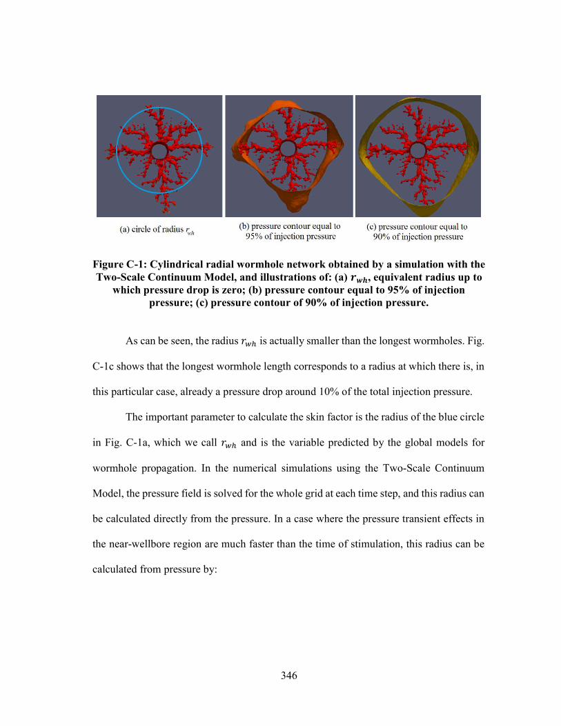
346

Figure C-1: Cylindrical radial wormhole network obtained by a simulation with the Two-Scale Continuum Model, and illustrations of: (a) 𝒓𝒘𝒉, equivalent radius up to

which pressure drop is zero; (b) pressure contour equal to 95% of injection pressure; (c) pressure contour of 90% of injection pressure.

As can be seen, the radius 𝑟 is actually smaller than the longest wormholes. Fig.

C-1c shows that the longest wormhole length corresponds to a radius at which there is, in

this particular case, already a pressure drop around 10% of the total injection pressure.

The important parameter to calculate the skin factor is the radius of the blue circle

in Fig. C-1a, which we call 𝑟 and is the variable predicted by the global models for

wormhole propagation. In the numerical simulations using the Two-Scale Continuum

Model, the pressure field is solved for the whole grid at each time step, and this radius can

be calculated directly from the pressure. In a case where the pressure transient effects in

the near-wellbore region are much faster than the time of stimulation, this radius can be

calculated from pressure by:

347

𝑟 (𝑡) = 𝑟𝑟

𝑟

( )

, (C.1)

where 𝑟 is the external radius of the simulation domain, 𝑝 is the pressure at the external

radius, 𝑝 (𝑡) is the injection pressure at any time 𝑡, and 𝑝 , is the initial injection

pressure. With time, as the wormholes propagate, 𝑝 (𝑡) decreases, corresponding to an

increase in 𝑟 that can be calculated with equation C.1. This is the radius of the

wormholed region plotted in Figure 3-25, and seen as a blue circle in Figure C-1a.

It is important to keep in mind that there are wormholes that are longer than this

average value. This can be seen in Fig. C-1a, and also in the experiments with large blocks

by McDuff et al. (2010) and Burton et al. (2018). In those experiments, only one wormhole

breaks through the block, while the other wormholes reach a smaller average length. When

one wormhole gets close enough to the border of the block it starts receiving more acid,

growing to the breakthrough.

This moment can be clearly seen in the pressure plot presented by McDuff et al.

(2010), evidenced by the pressure discontinuity at the end of the experiment (Figure

C-2b). The same behavior is seen in simulations using the Two-Scale Continuum Model.

Figure C-2 shows examples of the discontinuity for both a simulation (Figure C-2a) and

an experiment (Figure C-2b, published by McDuff et al., 2010). This discontinuity is not

expected in the field. It is an artifact of the experiments and simulations, because of the

existence of the borders. The global models of wormhole propagation are expected to

predict 𝑟 until before the discontinuity, but not the discontinuity itself.

348

Figure C-2: simulation and experimental pressure response showing the discontinuity at breakthrough

In field applications, the existence of wormholes longer than the average

wormhole length 𝑟 may be important when trying to avoid zones of undesired fluids,

such as aquifers or gas caps, or to avoid communicating different zones in intelligent

completions. In Fig. C-1, e.g., the longest wormhole is about 50% longer than 𝑟 .

349

APPENDIX D *

CALCULATION EXAMPLE USING THE NEW WORMHOLE GLOBAL MODEL

This section illustrates the calculation of the first time steps in the synthetic

example presented in section 3.2.4.1 (input in Table 3-7, results in Figure 3-26). The first

step in the procedure to calculate the wormhole propagation consists of calculating the

scaling factors 𝑓 and 𝑓 with equations (3.35) and (3.36):

𝑓 =𝑑

8 𝐿 𝑟 ,𝑟𝑒𝑝,

=1𝑖𝑛 ×

1𝑓𝑡12𝑖𝑛

8 × 1𝑓𝑡 × 3𝑓𝑡

.

= 0.115 (D.1)

𝑓 =𝑑

8 𝐿 𝑟 ,𝑟𝑒𝑝,

=1𝑖𝑛 ×

1𝑓𝑡12𝑖𝑛

8 × 1𝑓𝑡 × 1𝑓𝑡

.

= 0.109 (D.2)

These scaling factors 𝑓 and 𝑓 are assumed constant at their minimum values in

this example. The next step is to divide the injection time into steps, and at each time step

calculate the average interstitial velocity at the wormhole front, �̅� with equation (3.34),

and the velocity of the wormhole front, 𝑣 , with equation (3.28). Initially, at 𝑡 = 0, there

are no wormholes, so at the first time step 𝑟 = 𝑟 . In this example, 𝑟 = 0.328 𝑓𝑡, and

the average interstitial velocity �̅� at 𝑡 = 0 is given by:

* Part of this section is reprinted with permission from “Palharini Schwalbert, M., Hill, A. D., & Zhu, D. (2019c). A New Up-Scaled Wormhole Model Grounded on Experimental Results and in 2-Scale Continuum Simulations. Society of Petroleum Engineers. SPE-193616-MS.”

350

�̅� =𝑞

𝜙2𝜋𝐿𝑟𝑤ℎ=

60𝑏𝑝𝑚 × 5.615𝑓𝑡3/𝑏𝑏𝑙

0.15 × 2𝜋 × 1000𝑓𝑡 × 0.328𝑓𝑡= 1.1

𝑓𝑡

𝑚𝑖𝑛𝑢𝑡𝑒

= 33.2 𝑐𝑚

𝑚𝑖𝑛𝑢𝑡𝑒

(D.3)

𝑣 =𝑣𝑖

𝑃𝑉 , , × 𝑓×

𝑣𝑖

𝑣 , , × 𝑓

13

× 1 − exp −4𝑣𝑖

𝑣 , , × 𝑓

(D.4)

𝑣 =1.1𝑓𝑡/𝑚𝑖𝑛

0.51 × 0.115×

33.2𝑐𝑚/𝑚𝑖𝑛

2.16𝑐𝑚/𝑚𝑖𝑛 × 0.109

−13

× 1 − exp −433.2𝑐𝑚/𝑚𝑖𝑛

2.16𝑐𝑚/𝑚𝑖𝑛 × 0.109

2 2

(D.5)

𝑣 = 3.6 𝑓𝑡/𝑚𝑖𝑛 (D.6)

The velocity of the wormhole front at 𝑡 = 0 is 𝑣 = 3.6 𝑓𝑡/𝑚𝑖𝑛. We can now

calculate the radius of the wormholed region after the first time step ∆𝑡. The smaller the

time step ∆𝑡, the more accurate are the results. Using here a time step ∆𝑡 = 0.1 𝑚𝑖𝑛𝑢𝑡𝑒, the

radius of the wormholed region after 0.1 minute of acid injection is:

𝑟 (0.1𝑚𝑖𝑛) = 𝑟 (0) + ∆𝑡 × 𝑣 (0) = 0.328𝑓𝑡 + 0.1𝑚𝑖𝑛 × 3.6𝑓𝑡

𝑚𝑖𝑛

= 0.688𝑓𝑡

(D.7)

351

In the second time step, �̅� and 𝑣 must be recalculated using 𝑟 = 0.688𝑓𝑡:

�̅� =𝑞

𝜙2𝜋𝐿𝑟𝑤ℎ=

60𝑏𝑝𝑚 × 5.615𝑓𝑡3/𝑏𝑏𝑙

0.15 × 2𝜋 × 1000𝑓𝑡 × 0.688𝑓𝑡= 0.52

𝑓𝑡

𝑚𝑖𝑛𝑢𝑡𝑒

= 15.8𝑐𝑚

𝑚𝑖𝑛𝑢𝑡𝑒

(D.8)

𝑣 =0.52𝑓𝑡/𝑚𝑖𝑛

0.51 × 0.115×

15.8𝑐𝑚/𝑚𝑖𝑛

2.16𝑐𝑚/𝑚𝑖𝑛 × 0.109

−13

× 1 − exp −415.8𝑐𝑚/𝑚𝑖𝑛

2.16𝑐𝑚/𝑚𝑖𝑛 × 0.109

2 2

= 2.2𝑓𝑡/𝑚𝑖𝑛

(D.9)

𝑟 (0.2𝑚𝑖𝑛) = 𝑟 (0.1𝑚𝑖𝑛) + ∆𝑡 × 𝑣 (0.1) = 0.688𝑓𝑡 + 0.1𝑚𝑖𝑛 × 2.2𝑓𝑡

𝑚𝑖𝑛

= 0.91𝑓𝑡

(D.10)

This procedure is repeated until the total injection time: at each time step, �̅� and

𝑣 are recalculated using the most current 𝑟 (𝑡), then 𝑟 (𝑡 + ∆𝑡) is calculated. This is

easily implemented in any spreadsheet. In this synthetic example, after the total injection

time of 29.7 minutes, the result is 𝑟 = 14.2𝑓𝑡. The skin factor can then be calculated with

equation (3.51):

𝑠 = − ln𝑟

𝑟= − ln

14.2

0.328= −3.8

(D.11)

352

APPENDIX E *

COMPARISON OF THE REQUIRED PERFORATION SPACING FOR THE SAME

STIMULATION COVERAGE IN ANISOTROPIC AND ISOTROPIC FORMATIONS

In limited entry completions, each acid entry point creates one ellipsoidal

wormhole network, such as illustrated in Figure 3-34. The stimulated volume per foot is

the volume of one ellipsoid divided by the perforation spacing:

𝑉

ℎ=

4𝜋𝑅 𝑅

3ℎ=

4𝜋𝑅

3ℎ 𝐼 ,

(E.1)

The equivalent relation for the isotropic case is:

𝑉

ℎ=

4𝜋𝑅

3ℎ

(E.2)

By joining the definition of the stimulation coverage for a vertical well, equation

(3.56), with the definition of the wormhole anisotropy ratio, equation (3.53), it can be

written:

* Part of this section is reprinted with permission from “Palharini Schwalbert, M., Hill, A. D., & Zhu, D. (2019b, January 1). Skin-Factor Equations for Anisotropic Wormhole Networks and Limited-Entry Completions. Society of Petroleum Engineers. doi:10.2118/189486-PA”

353

𝑅 =𝐶 ℎ 𝐼 ,

2

(E.3)

Substituting equation E.3 into E.1:

𝑉

ℎ=

𝜋

6𝐶 ℎ 𝐼 ,

(E.4)

Analogously, for the isotropic case:

𝑉

ℎ=

𝜋

6𝐶 ℎ

(E.5)

Hence, for the same stimulated volume, one can compare the isotropic and

anisotropic cases by equating Eq. E.4 and E.5:

𝜋

6𝐶 ℎ 𝐼 , =

𝜋

6𝐶 ℎ (E.6)

To obtain the same stimulation coverage, the relation between the perforation

spacing required for the anisotropic and the isotropic cases is given by:

ℎ

ℎ=

1

𝐼 , (𝑣𝑒𝑟𝑡𝑖𝑐𝑎𝑙 𝑤𝑒𝑙𝑙)

(E.7)

354

On the other hand, if the same perforation spacing is used in both anisotropic and

isotropic formations, but still the same stimulation coverage is sought, then the stimulated

volume per foot must not be the same for both cases. In this case, equation E.6 would not

be valid. Isolating ℎ from equations E.4 and E.5 results:

ℎ =𝑉

ℎ

6

𝜋𝐶 𝐼 ,

(𝑣𝑒𝑟𝑡𝑖𝑐𝑎𝑙 𝑤𝑒𝑙𝑙) (E.8)

ℎ =𝑉

ℎ

6

𝜋𝐶 (𝑣𝑒𝑟𝑡𝑖𝑐𝑎𝑙 𝑤𝑒𝑙𝑙)

(E.9)

In this case, if the same perforation spacing ℎ is used for both anisotropic and

isotropic cases, the relation between the stimulated volumes that must be obtained in each

case to result in the same stimulation coverage is found by making equations E.8 and E.9

equal:

(𝑉 )

(𝑉 )= 𝐼 , (𝑣𝑒𝑟𝑡𝑖𝑐𝑎𝑙 𝑤𝑒𝑙𝑙)

(E.10)

If the overall acid efficiency is the same in both cases, resulting in the same overall

𝑃𝑉 , then equation E.10 can be rewritten as:

355

(𝑉 )

(𝑉 )= 𝐼 , (𝑣𝑒𝑟𝑡𝑖𝑐𝑎𝑙 𝑤𝑒𝑙𝑙)

(E.11)

The same analysis can be made for a horizontal well. The difference is that in this

case, if the horizontal permeability is larger than the vertical, the wormholes grow longer

in the horizontal direction in the anisotropic case. For the horizontal well, the definition

of the stimulation coverage is given by equation (3.57), from which it can be written:

𝑅 =𝐶 ℎ

2

(E.12)

𝑉

𝐿=

𝜋

6

𝐶 ℎ

𝐼 ,

(E.13)

𝑉

𝐿=

𝜋

6𝐶 ℎ

(E.14)

Hence, for the same stimulated volume, one can compare the isotropic and

anisotropic cases by equating Eq. E.13 and E.14:

𝜋

6

𝐶 ℎ

𝐼 ,=

𝜋

6𝐶 ℎ (E.15)

To obtain the same stimulation coverage, the relation between the perforation

spacing required for the anisotropic and the isotropic cases is given by:

356

ℎ

ℎ= 𝐼 , (ℎ𝑜𝑟𝑖𝑧𝑜𝑛𝑡𝑎𝑙 𝑤𝑒𝑙𝑙)

(E.16)

On the other hand, if the same perforation spacing is used in both anisotropic and

isotropic formations, but still the same stimulation coverage is sought, then the stimulated

volume per foot must not be the same for both cases. In this case, equation E.15 would not

be valid. Isolating ℎ from equations E.13 and E.14 results:

ℎ =𝑉

𝐿

6𝐼 ,

𝜋𝐶 (ℎ𝑜𝑟𝑖𝑧𝑜𝑛𝑡𝑎𝑙 𝑤𝑒𝑙𝑙)

(E.17)

ℎ =𝑉

𝐿

6

𝜋𝐶 (ℎ𝑜𝑟𝑖𝑧𝑜𝑛𝑡𝑎𝑙 𝑤𝑒𝑙𝑙)

(E.18)

In this case, if the same perforation spacing ℎ is used for both anisotropic and

isotropic cases, the relation between the stimulated volumes that must be obtained in each

case to result in the same stimulation coverage is found by equating Eq. E.17 and E.18:

(𝑉 )

(𝑉 )=

1

𝐼 , (ℎ𝑜𝑟𝑖𝑧𝑜𝑛𝑡𝑎𝑙 𝑤𝑒𝑙𝑙) (E.19)

If the overall acid efficiency is the same in both cases, resulting in the same overall

𝑃𝑉 , then equation E.19 can be rewritten as:

357

(𝑉 )

(𝑉 )=

1

𝐼 , (ℎ𝑜𝑟𝑖𝑧𝑜𝑛𝑡𝑎𝑙 𝑤𝑒𝑙𝑙) (E.20)

358

APPENDIX F *

DERIVATION OF A SKIN FACTOR EQUATION FOR A LIMITED ENTRY

STIMULATION IN VERTICAL WELLS

The derivation is performed assuming steady state in a cylindrical drainage region

with external radius 𝑟 . For this geometry, there is radial flow from the outer boundary

until some distance from the well where the flow becomes spherical/ellipsoidal,

converging to the perforations. This is illustrated in Figure F-1, and a simulation result

showing this behavior in isobars is shown in Figure F-2.

Figure F-1: Illustration of flow pattern from cylindrical reservoir to vertical well stimulated with limited entry technique.

* Part of this section is reprinted with permission from “Palharini Schwalbert, M., Hill, A. D., & Zhu, D. (2019b, January 1). Skin-Factor Equations for Anisotropic Wormhole Networks and Limited-Entry Completions. Society of Petroleum Engineers. doi:10.2118/189486-PA”

359

(a)

(b)

Figure F-2: Pressure contours. (a) Overview of the flow in the reservoir. (b) Detail of the transition from radial to ellipsoidal flow at a distance 𝒉𝒑𝒆𝒓𝒇𝑰𝒂𝒏𝒊/𝟐 from the

wellbore. The pressure drop is given by:

∆𝑝 =𝑞 𝐵𝜇

2𝜋𝑘 ℎln

𝑟

𝑟+ 𝑠 (F.1)

360

where 𝑞 is the flow rate produced by each perforation. The pressure drop can be also

given by the sum of two components: radial, ∆𝑝 , and ellipsoidal, ∆𝑝 :

∆𝑝 = ∆𝑝 + ∆𝑝 (F.2)

There is radial flow from the outer boundary until the flow pattern starts to

converge to the perforations, which happens at a distance ℎ 𝐼 /2 from the well. The

pressure drop in the radial flow regions is:

∆𝑝 =𝑞 𝐵𝜇

2𝜋𝑘 ℎln

𝑟

ℎ 𝐼 /2

(F.3)

The pressure drop in the ellipsoidal flow is calculated in analogy with the spherical

flow. For a spherical flow from a radius 𝑅 to a radius 𝑅 , the pressure drop is given by:

∆𝑝 =𝑞𝐵𝜇

4𝜋𝑘

1

𝑅 −

1

𝑅 (F.4)

where 𝑘 is the spherical permeability, which in a reservoir with a vertical permeability

𝑘 and two equal horizontal permeabilities 𝑘 is given by:

361

𝑘 = 𝑘 𝑘 𝑘 = 𝑘 𝑘 (F.5)

Analogously to Eq. F.4, the pressure drop in ellipsoidal flow is given by:

∆𝑝 =𝑞𝐵𝜇

4𝜋 𝑘 𝑘/

1

𝑅 −

1

𝑅 (F.6)

where the equivalent radii 𝑅 and 𝑅 are related to the inner and outer ellipsoids’

major semi-axes by:

𝑅 =𝑅

𝐼 ,/

(F.7)

where 𝐼 , is the ratio between major and minor semi-axes of the ellipsoid, as defined

by equation (3.53). For calculating the ellipsoidal flow region pressure drop, it is still

necessary to define the outer and inner ellipsoids where the flow happens. Here two

assumptions are made.

The inner boundary is given by the usual assumption in carbonate acidizing: it is

considered that the wormholed region has permeability infinitely greater than the reservoir

permeability, so that the pressure drop from the tip of the wormholes to the perforation is

negligible. Hence, the inner ellipsoid is the stimulated region itself.

362

For the outer ellipsoid, an assumption must be made, as the inner radius of the

radial flow region defines actually a cylinder, and not an ellipsoid. There is a transition

region from the cylindrical radial flow to the ellipsoidal flow. Radial flow occurs until the

radius ℎ 𝐼 /2. The ellipsoid that fits inside this cylinder has major semi-axis 𝑅

given by Eq. F.8, while the ellipsoid that circumscribes that cylinder has major semi-axis

𝑅 given by Eq. F.9. Both ellipsoids are illustrated in Figure F-3.

𝑅 =ℎ 𝐼

2

(F.8)

𝑅 =ℎ 𝐼

2√2

(F.9)

Figure F-3: Illustration of bounding ellipsoids in ellipsoidal flow region.

363

Assuming ellipsoidal flow only from 𝑅 to 𝑅 would underestimate the

pressure drop, because it would leave a part of the reservoir out of the calculation.

However, assuming ellipsoidal flow all the way from 𝑅 to 𝑅 would overestimate

the pressure drop, because it would count twice for a region of the reservoir. Hence, the

assumption chosen here and tested to be a good option is considering ellipsoidal flow from

an average radius between 𝑅 and 𝑅 :

𝑅 =ℎ 𝐼

2

1 + √2

2

(F.10)

Finally, the pressure drop in the region of ellipsoidal flow is:

∆𝑝 =𝑞 𝐵𝜇

4𝜋 𝑘 𝑘/

𝐼/

𝑅 −

4𝐼/

ℎ 𝐼 1 + √2 (F.11)

Substituting Eq. F.11 and F.3 into Eq. F.2 and grouping some terms results in:

∆𝑝 =𝑞 𝐵𝜇

2𝜋𝑘 ℎln

2𝑟

ℎ 𝐼 +

ℎ 𝐼

2𝑅−

2

1 + √2

(F.12)

Finally, comparing equations F.12 and F.1, the skin factor for this vertical well

stimulated with a limited entry technique is found to be:

364

𝑠 =ℎ 𝐼

2𝑅−

2

1 + √2− ln

ℎ 𝐼

2𝑟

(F.13)

And the total flow rate for the well can be directly calculated by:

𝑞 =2𝜋𝑘 ℎ∆𝑝

𝐵𝜇 ln2𝑟

ℎ 𝐼 +

ℎ 𝐼2𝑅

−2

1 + √2

(F.14)

365

APPENDIX G *

DERIVATION OF A SKIN FACTOR EQUATION FOR A LIMITED ENTRY

STIMULATION IN HORIZONTAL WELLS

This derivation is performed in a way very similar to that of the vertical well in

Appendix F, except that the starting point is a fully penetrating horizontal well in a

rectangular reservoir and Furui’s horizontal well inflow model is used for comparison.

The pressure drop is given by:

∆𝑝 =𝑞𝐵𝜇

2𝜋𝑘𝐿ln

ℎ𝐼 √2

𝑟 (𝐼 + 1)+ 𝜋

𝑦

ℎ𝐼−

1

2 + 𝑠

(G.1)

where 𝐿 is the well length, 𝑦 is half the well spacing or the distance from the well to the

outer boundary of the drainage region orthogonal to the well, and 𝑘 is the geometric mean

permeability:

𝑘 = 𝑘 𝑘 (G.2)

* Part of this section is reprinted with permission from “Palharini Schwalbert, M., Hill, A. D., & Zhu, D. (2019b, January 1). Skin-Factor Equations for Anisotropic Wormhole Networks and Limited-Entry Completions. Society of Petroleum Engineers. doi:10.2118/189486-PA”

366

Equation G.1 is derived by considering two regions of flow in the reservoir: a linear

flow from the outer boundary until some point where the flow starts to become

radial/elliptical to converge to the wellbore. In the well stimulated with limited entry, there

are not two, but three regions: (1) linear flow from the outer boundary, (2) radial/elliptical

flow converging to the well, and (3) spherical/ellipsoidal flow converging to the

ellipsoidal wormhole network.

The boundaries where each one of these regions starts or ends depend on some

relations between the perforation spacing ℎ , the formation thickness ℎ, and the

wormhole length 𝑅 . For ℎ ≤ ℎ𝐼 , e.g., there is linear flow from the outer

reservoir boundary until the horizontal distance ℎ𝐼 /2 from the well. From this point

there is elliptical flow until the horizontal distance ℎ /2 from the well, where the

ellipsoidal flow starts. The ellipsoidal flow goes from the horizontal distance ℎ /2 until

the wormholed region, which is at a distance 𝑅 from the well. The total pressure drop,

in this case, is the sum of the pressure drop in each of the three regions:

∆𝑝 = ∆𝑝 + ∆𝑝 + ∆𝑝 (G.3)

∆𝑝 =𝑞𝐵𝜇

2𝜋𝑘𝐿

𝜋

ℎ𝐼𝑦 −

ℎ𝐼

2

(G.4)

∆𝑝 = 𝑞𝐵𝜇

2𝜋𝑘𝐿ln

ℎ𝐼 √2

ℎ

(G.5)

∆𝑝 = 𝑞𝐵𝜇

2𝜋𝑘𝐿

ℎ

2𝑅−

2

1 + √2

(G.6)

367

Grouping all terms and comparing to Eq. G.1, the skin factor is obtained:

𝑠 =ℎ

2𝑅−

2

1 + √2− ln

ℎ

𝑟 (𝐼 + 1)

(G.7)

Analogously, for cases with aggressive limited entry completion, hence a large

perforation spacing ℎ > ℎ𝐼 , there is linear flow from the outer reservoir boundary

until the horizontal distance ℎ /2 from the well. From this point, if the wormhole

length is such that 𝑅 < ℎ𝐼 /2, there is cylindrical radial flow until the horizontal

distance ℎ𝐼 /2 from the well, where the ellipsoidal flow starts. The ellipsoidal flow goes

from the horizontal distance ℎ𝐼 /2 until the wormholed region, which is at a distance

𝑅 from the well. The total pressure drop, in this case, is again the sum of the three

parts, but each part is different because the boundaries between the regions are different:

∆𝑝 = ∆𝑝 + ∆𝑝 + ∆𝑝 (G.8)

∆𝑝 =𝑞𝐵𝜇

2𝜋𝑘𝐿

𝜋

ℎ𝐼𝑦 −

ℎ

2

(G.9)

∆𝑝 = 𝑞𝐵𝜇

2𝜋𝑘𝐿

ℎ

ℎ𝐼ln

ℎ √2

ℎ𝐼

(G.10)

∆𝑝 = 𝑞𝐵𝜇

2𝜋𝑘𝐿

ℎ

2𝑅−

ℎ

ℎ𝐼

2

1 + √2

(G.11)

368

Grouping all terms and comparing to Eq. G.1, the skin factor is obtained:

𝑠 =ℎ

2𝑅−

2

1 + √2

ℎ

ℎ𝐼+

𝜋

21 −

ℎ

ℎ𝐼+

ℎ

ℎ𝐼ln

ℎ √2

ℎ𝐼

− lnℎ𝐼 √2

𝑟 (𝐼 + 1)

(G.12)

The same reasoning can be applied to the case with large perforation spacing,

ℎ > ℎ𝐼 , and long wormholes, 𝑅 ≥ (the wormholes reach the whole

formation thickness in the vertical direction), to find the skin factor:

𝑠 =𝜋

21 −

ℎ

ℎ𝐼+

ℎ

ℎ𝐼ln

ℎ √2

2𝑟∗ − lnℎ𝐼 √2

𝑟 (𝐼 + 1)

(G.13)

where 𝑟∗ is the horizontal length of the equivalent elliptical wormholed region after the

wormhole networks interconnect, as discussed in section 3.3.3.2.

369

APPENDIX H *

SKIN FACTOR AS A FUNCTION OF THE STIMULATION COVERAGE FOR A

LIMITED ENTRY COMPLETION

As shown in Figure 3-35, in a vertical well stimulated using a limited entry scheme,

for a given stimulated volume per foot, it seems the skin factor should be a function of

only the stimulation coverage. This can be shown starting with equation (3.66), and

substituting the wormhole length, 𝑅 , and the perforation spacing, ℎ , by their

relation with the stimulation coverage, 𝐶 , and the stimulated volume per foot, .

From Eq. E.3, assuming 𝐼 , = 𝐼 , it results:

ℎ 𝐼 =2𝑅

𝐶

(H.1)

By substituting Eq. E.3 and H.1 into E.1, and isolating 𝑅 :

𝑅 = 𝑉

ℎ

3

2𝜋𝐶

(H.2)

* Part of this section is reprinted with permission from “Palharini Schwalbert, M., Hill, A. D., & Zhu, D. (2019b, January 1). Skin-Factor Equations for Anisotropic Wormhole Networks and Limited-Entry Completions. Society of Petroleum Engineers. doi:10.2118/189486-PA”

370

Finally, substituting Eq. H.1 and H.2 into equation (3.66), it results:

𝑠 =1

𝐶−

2

1 + √2− ln

⎝

⎛

𝑉ℎ

32𝜋𝐶

𝐶 𝑟

⎠

⎞, (𝑣𝑒𝑟𝑡𝑖𝑐𝑎𝑙 𝑤𝑒𝑙𝑙, 𝐶 ≤ 1) (H.3)

The same analysis can be done for a horizontal well. In this case, if ℎ ≤ ℎ𝐼

(most common case), equation (3.69) should be used. Again, it is useful to eliminate the

wormhole length, 𝑅 , and the perforation spacing, ℎ , by their relation with the

stimulation coverage, 𝐶 , and the stimulated volume per foot, . Substituting

equations E.12 and E.17 into (3.69) and assuming 𝐼 , = 𝐼 results in:

𝑠 =1

𝐶−

2

1 + √2− ln

⎣⎢⎢⎡2

𝑉𝐿

32𝜋

𝐼𝐶

𝑟 𝐶 (𝐼 + 1)

⎦⎥⎥⎤

, (ℎ𝑜𝑟𝑖𝑧𝑜𝑛𝑡𝑎𝑙 𝑤𝑒𝑙𝑙, 𝐶 ≤ 1) (H.4)

In this case, 𝐼 does not cancel completely, and the resulting skin factor is a

function of the anisotropy ratio.

371

APPENDIX I

PARAMETERS “A” AND “B” FOR COMMON ACID FRACTURE

CONDUCTIVITY CORRELATIONS

In section 4.5, the acid fracture conductivity correlation was presented in the

generalized form of equation (4.66), repeated here without the average symbol:

𝑘 𝑤 = 𝐴𝑤 (I.1)

This Appendix presents the form of the coefficients 𝐴 and 𝐵 for four different

conductivity models: Nierode and Kruk (1973), Deng et al. (2012), Neumann (2011), and

Nasr-El-Din (2008). Although these correlations are different in form and origin, they can

all be written as equation (I.1), with similar values of 𝐵 (the same applies to the models

by Gangi (1978), Gong et al. (1999), and Pournik et al. (2009), not presented here).

I.1 Nierode and Kruk (1973) correlation

For the model by Nierode and Kruk (1973), 𝐵 = 2.466, and 𝐴 is given in field

units (md-ft-in-2.47) by:

372

𝐴 =1.476 × 10 exp[−0.001[13.9 − 1.3 ln(𝑆 )]𝜎 ] , 𝑖𝑓 𝑆 < 20,000 𝑝𝑠𝑖

1.476 × 10 exp[−0.001[3.8 − 0.28 ln(𝑆 )]𝜎 ] , 𝑖𝑓 𝑆 ≥ 20,000 𝑝𝑠𝑖

(I.2)

where 𝜎 is the effective confining stress in psi – equation (4.86) –, and 𝑆 is the rock

embedment strength in psi.

I.2 Deng et al. (2012) correlation

This correlation has several different forms. All of them can be written in the form

of equation (I.1). Deng et al. (2012) presented the correlation in the form:

𝑘 𝑤 = 𝛼 exp(−𝛽𝜎 ′) (I.3)

In general, 𝐵 is the power to which 𝑤 is raised in the equations (ranging from

2.43 to 2.52), and 𝐴 is given in by:

𝐴 =𝛼 exp(−𝛽𝜎 ′)

𝑤

(I.4)

It is important to notice that 𝐴 does not depend on 𝑤 . Even though 𝑤 appears in

the equation above, it actually cancels the term 𝑤 that appears in 𝛼, so that the resulting

373

coefficient 𝐴 is a constant for a given formation. All the dependence of the conductivity

on the etched width is in the term 𝑤 . Each case of Deng et al. (2012) correlation is

analyzed in the following, with a value for 𝐵 and an explicit equation for 𝐴 for each

scenario. What is called 𝑤 (standing for etched width) in this study is the same quantity

called 𝑤 (standing for ideal width) by Deng et al. (2012).

I.2.1 Permeability-Distribution-Dominant Cases with High Leakoff

For high leakoff coefficient (𝐶 ≳ 0.004 𝑓𝑡/√𝑚𝑖𝑛), 𝐵 = 2.49, and 𝐴 is given in

field units (md-ft-in-2.49) by:

𝐴 = 4.48 × 10 × [0.56 erf(0.8𝜎 )]

× 0.22 𝜆 , 𝜎.

+ 0.01 1 − 𝜆 , 𝜎. .

× 1 +1.82 erf 3.25 𝜆 , − 0.12 +

−1.31 erf 6.71 𝜆 , − 0.03× √𝑒 − 1

× exp[−(14.9 − 3.78 ln 𝜎 − 6.81 ln 𝐸) × 10 × 𝜎 ]

(I.5)

where 𝐸 is the rock’s Young’s modulus in Mpsi, 𝜎 is the normalized standard deviation

of the permeability distribution, 𝜆 , and 𝜆 , are the normalized horizontal (x) and

vertical (z) correlation lengths of the permeability distributions.

374

I.2.2 Permeability-Distribution-Dominant Cases with Medium Leakoff

This case applies when the leakoff coefficient is not so large as the previous case,

but the conductivity is still dominated by the permeability distribution. Deng et al. (2012)

recommends this for cases where C ~0.001 ft/√min with uniform mineralogy

distribution. In this case, 𝐵 = 2.43, and 𝐴 is given in field units (md-ft-in-2.43) by:

𝐴 = 4.48 × 10 × [0.2 erf(0.78𝜎 )]

× 0.22 𝜆 , 𝜎.

+ 0.01 1 − 𝜆 , 𝜎. .

× 1 +1.82 erf 3.25 𝜆 , − 0.12

−1.31 erf 6.71 𝜆 , − 0.03× √𝑒 − 1

× exp[−(14.9 − 3.78 ln 𝜎 − 6.81 ln 𝐸) × 10 × 𝜎 ]

(I.6)

I.2.3 Mineralogy-Distribution-Dominant Cases

When the leakoff coefficient is low (𝐶 ≲ 0.0004 𝑓𝑡/√𝑚𝑖𝑛), Deng et al. (2012)

recommend the use of a correlation which is a function of the mineralogy distribution

instead of permeability statistical parameters. The presented correlation considered only

calcite and dolomite as present minerals, and the equations are only in function of the

fraction of calcite. In this case, 𝐵 = 2.52, and 𝐴 is given in field units (md-ft-in-2.52) by:

375

𝐴 = 4.48 × 10 0.13𝑓 . [1 + 2.97(1 − 𝑓 ) . ]

× (0.811 − 0.853𝑓 )

× exp{−[1.2 exp(0.952𝑓 ) + 10.5𝐸 . ] × 10 × 𝜎 }

(I.7)

where 𝑓 is the fraction of calcite.

I.2.4 Competing Effects of Permeability and Mineralogy Distributions

When the leakoff coefficient is medium (𝐶 ~0.001 𝑓𝑡/√𝑚𝑖𝑛), both permeability

and mineralogy have competing effects on the conductivity. In this case, 𝐵 = 2.52, and 𝐴

is given in field units (md-ft-in-2.52) by:

𝐴 = 4.48 × 10 (0.1𝑓 . + 0.14𝜎 )

× 1.2 +erf 5 𝜆 , − 0.12 +

−0.6 erf 3.5 𝜆 , − 0.03√𝑒 − 1

× 0.21𝜆 ,. + 0.15𝜆 ,

. + 0.046 ln(𝜎 )

× exp[−(53.8 + 18.9 ln 𝜎 − 4.58 ln 𝐸) × 10 × 𝜎 ]

(I.8)

The correlations presented by Deng et al. (2012) are valid when: 𝐸 > 1 𝑀𝑝𝑠𝑖,

𝜎 > 500 𝑝𝑠𝑖, 0.156 ≤ 𝜆 , ≤ 1, 0.004 ≤ 𝜆 , ≤ 0.5, and 0.1 ≤ 𝜎 ≤ 0.9.

376

I.3 Neumann (2011) correlation

Neumann (2011) measured experimentally the conductivity of acid fractures with

deep microbial carbonates, and proposed a correlation similar to Nierode and Kruk (1973),

with dependence only on rock embedment strength, 𝑆 , and effective confining stress,

𝜎 . With Neumann (2011)’s correlation, 𝐵 = 2.508, and 𝐴 is given in field units (md-ft-

in-2.508) by:

𝐴 = 1.693 × 10 exp−𝜎

−4790 + 568 ln(𝑆 )

(I.9)

where 𝜎 and 𝑆 are in psi.

I.4 Nasr-El-Din et al. (2008) correlations

Nasr-El-Din et al. (2008) reevaluated the experimental data by Nierode and Kruk

(1973), and recommend using different equations for the conductivity of acid fractures in

limestones and dolomites. For limestones, they recommend 𝐵 = 2.624, and 𝐴 given in

field units (md-ft-in-2.624) by:

377

𝐴 =3.374 × 10 exp[−0.001[26.6 − 8.6 ln(𝑆 )]𝜎 ] , 𝑖𝑓 𝑆 < 20,000 𝑝𝑠𝑖

3.374 × 10 exp[−0.001[2.98 − 0.2 ln(𝑆 )]𝜎 ] , 𝑖𝑓 𝑆 ≥ 20,000 𝑝𝑠𝑖

(I.10)

For dolomites, Nasr-El-Din et al. (2008) recommend 𝐵 = 1.68, and 𝐴 given in

field units (md-ft-in-1.68) by:

𝐴 =1.12 × 10 exp[−0.001[8.64 − 0.75 ln(𝑆 )]𝜎 ] , 𝑖𝑓 𝑆 < 20,000 𝑝𝑠𝑖

1.12 × 10 exp[−0.001[2.315 − 0.15 ln(𝑆 )]𝜎 ] , 𝑖𝑓 𝑆 ≥ 20,000 𝑝𝑠𝑖

(I.11)