Complex Patterns

in Reaction-Di�usion Systems:

A Tale of Two Front Instabilities

Aric Hagberg

Program in Applied Mathematics

University of Arizona, Tucson, AZ 85721

Ehud Meron

Arizona Center for Mathematical Sciences

Department of Mathematics

University of Arizona, Tucson, AZ 85721

May 16, 1994

Abstract

Two front instabilities in a reaction-di�usion system are shown to lead to the for-

mation of complex patterns. The �rst is an instability to transverse modulations that

drives the formation of labyrinthine patterns. The second is a Nonequilibrium Ising-

Bloch (NIB) bifurcation that renders a stationary planar front unstable and gives rise

to a pair of counterpropagating fronts. Near the NIB bifurcation the relation of the

front velocity to curvature is highly nonlinear and transitions between counterprop-

agating fronts become feasible. Nonuniformly curved fronts may undergo local front

transitions that nucleate spiral-vortex pairs. These nucleation events provide the ingre-

dient needed to initiate spot splitting and spiral turbulence. Similar spatio-temporal

processes have been observed recently in the ferrocyanide-iodate-sul�te reaction.

1

1 Introduction

Labyrinthine patterns, spot replication, and spiral wave turbulence are all examples

of complex spatial and spatiotemporal patterns exhibited in reaction-di�usion systems.

Labyrinthine patterns have been observed in a variety of gradient systems including gar-

net layers [1], ferro uids [2], and block copolymers [3, 4]. Recently they also were found

in the bistable FIS (ferrocyanide-iodate-sul�te) reaction [5]. This nongradient system also

exhibits spot replication and spiral turbulence [6].

Much of this phenomenology can be understood in terms of two key front instabilities:

an instability to transverse perturbations reminiscent of the Mullins-Sekerka instability in

solidi�cation fronts [7], and a nonequilibrium analog of the Ising-Bloch transition in ferro-

magnets that we call a Nonequilibrium Ising-Bloch (NIB) front bifurcation [8, 9]. At a NIB

bifurcation, a stationary \Ising" front bifurcates to a pair of \Bloch" fronts propagating in

opposite directions. The coexistence of counterpropagating fronts is a nongradient e�ect that

lies at the heart of the complex spatio-temporal processes. Beyond the transverse instability

and deep in the Ising regime labyrinthine patterns may develop when small disturbances

on planar Ising fronts grow and �ll the system through �ngering and tip splitting. In the

vicinity of the NIB bifurcation intrinsic perturbations, such as curvature, may drive dynamic

transitions between the two counterpropagating fronts and lead to spot splitting and spiral

breakup [10].

To study these instabilities we consider a nongradient doubly di�usive reaction-di�usion

model for two scalar �elds u and v:

u

t

= u� u

3

� v +r

2

u; (1.1a)

v

t

= �(u� a

1

v � a

0

) + �r

2

v: (1.1b)

This type of model has been studied in the context of nerve conduction (with � = 0) and

chemical reactions [11, 12], semiconductor etalons [13], and many other systems [14]. For

� � 1 it reduces to a gradient system like those studied in the context of phase separating

systems [15, 16].

Equations (1.1) contain four parameters: �, the ratio of the time scales associated with

the two �elds, �, the ratio of the di�usion constants, and two parameters, a

1

> 0 and a

0

,

that determine the number and type of homogeneous steady states. These states are found

by the intersections of the nullclines v = u � u

3

and v = (u � a

0

)=a

1

. For this study we

always choose a

1

and a

0

so there are three intersections, each on a di�erent branch of the

cubic nullcline. The intersections on the outer branches represent stable solutions which we

will call (u

+

; v

+

) for the positive branch \up" state, and (u

�

; v

�

) for the negative branch

\down" state. When a

0

=0 equations (1.1) have an odd symmetry and (u

+

; v

+

) = �(u

�

; v

�

).

We focus in this paper on the regime �=� � 1 where a singular perturbation analysis

of (1.1) can be performed. In section 2 we review the derivation of the Ising-Bloch front

2

bifurcation line in the ��� parameter plane [17, 18]. In section 3 we investigate the stability of

planar Ising and Bloch fronts to transverse perturbations. Implications of the two instabilities

on the formation of labyrinthine patterns, spot splitting, and spiral turbulence are studied in

section 4. Section 5 contains a description of the numerical methods used in the simulations

and Section 6 concludes by connecting this work to a few others.

2 The NIB Bifurcation

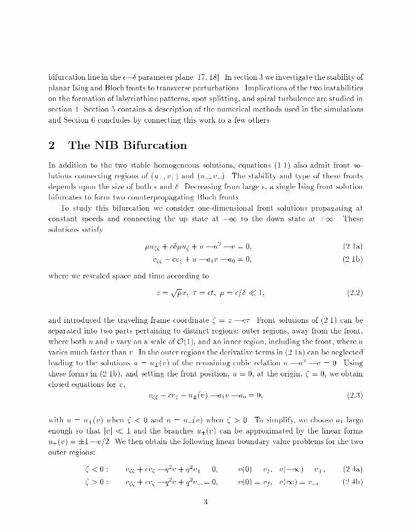
In addition to the two stable homogeneous solutions, equations (1.1) also admit front so-

lutions connecting regions of (u

+

; v

+

) and (u

�

; v

�

). The stability and type of these fronts

depends upon the size of both � and �. Decreasing from large �, a single Ising front solution

bifurcates to form two counterpropagating Bloch fronts.

To study this bifurcation we consider one-dimensional front solutions propagating at

constant speeds and connecting the up state at �1 to the down state at +1. These

solutions satisfy

�u

��

+ c��u

�

+ u� u

3

� v = 0; (2.1a)

v

��

+ cv

�

+ u� a

1

v � a

0

= 0; (2.1b)

where we rescaled space and time according to

z =

p

�x; � = �t; � = �=�� 1; (2:2)

and introduced the traveling frame coordinate � = z � c� . Front solutions of (2.1) can be

separated into two parts pertaining to distinct regions: outer regions, away from the front,

where both u and v vary on a scale of O(1), and an inner region, including the front, where u

varies much faster than v. In the outer regions the derivative terms in (2.1a) can be neglected

leading to the solutions u = u

�

(v) of the remaining cubic relation u � u

3

� v = 0. Using

these forms in (2.1b), and setting the front position, u = 0, at the origin, � = 0, we obtain

closed equations for v,

v

��

+ cv

�

+ u

�

(v)� a

1

v � a

0

= 0; (2:3)

with u = u

+

(v) when � < 0 and u = u

�

(v) when � > 0. To simplify, we choose a

1

large

enough so that jvj � 1 and the branches u

�

(v) can be approximated by the linear forms

u

�

(v) = �1�v=2. We then obtain the following linear boundary value problems for the two

outer regions:

� < 0 : v

��

+ cv

�

� q

2

v + q

2

v

+

= 0; v(0) = v

f

; v(�1) = v

+

; (2.4a)

� > 0 : v

��

+ cv

�

� q

2

v + q

2

v

�

= 0; v(0) = v

f

; v(1) = v

�

; (2.4b)

3

where

v

�

=

�1� a

0

a

1

+ 1=2

; q

2

= a

1

+ 1=2; (2.5a)

and v

f

is the level of v at the front position. The solutions are

v(�) = (v

f

� v

+

)e

�

1

�

+ v

+

; � < 0; (2.6a)

v(�) = (v

f

� v

�

)e

�

2

�

+ v

�

; � > 0; (2.6b)

with

�

1;2

= �c=2 � (c

2

=4 + q

2

)

1=2

: (2:7)

By construction, the two outer solutions for v are continuous at � = 0. Matching the

derivatives of v at � = 0 gives a relation between c, the speed of the front, and v

f

, the value

of the v �eld at the front position,

v

f

= �

c

2q

2

(c

2

=4 + q

2

)

1=2

�

a

0

q

2

: (2:8)

A second relation between v

f

and c is obtained by solving the inner problem. In the front

region u varies on a scale of O(

p

�) but variations of v are still on a scale of O(1). Stretching

the traveling-frame coordinate according to � = �=

p

� we obtain from (2.1)

u

��

+ �cu

�

+ u� u

3

� v = 0; (2.9a)

v

��

+

p

�cv

�

+ �(u� a

1

v � a

0

) = 0; (2.9b)

where �

2

= ��. Setting � = 0 in (2.9b) gives the equation v

��

= 0, and we choose the

solution v = constant. Fixing the constant, v = v

f

, in the equation for u gives a nonlinear

eigenvalue problem for c,

u

��

+ �cu

�

+ f(u; v

f

) = 0; (2.10a)

u(�1) = u

�

(v

f

); (2.10b)

with f(u; v

f

) = u� u

3

� v

f

. The cubic function, f , can be rewritten as

f(u; v

f

) = �[u� u

�

(v

f

)][u� u

0

(v

f

)][u� u

+

(v

f

)]; (2:11)

where u

�

(v

f

) = �1 � v

f

=2; u

0

= v

f

; and u

+

(v

f

) = 1 � v

f

=2; are the linearized forms of

4

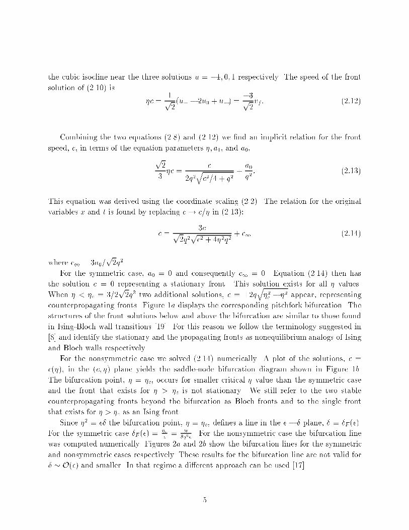
the cubic isocline near the three solutions u = �1; 0; 1 respectively. The speed of the front

solution of (2.10) is

�c =

1

p

2

(u

+

� 2u

0

+ u

�

) =

�3

p

2

v

f

: (2:12)

Combining the two equations (2.8) and (2.12) we �nd an implicit relation for the front

speed, c, in terms of the equation parameters �; a

1

; and a

0

,

p

2

3

�c =

c

2q

2

q

c

2

=4 + q

2

+

a

0

q

2

: (2:13)

This equation was derived using the coordinate scaling (2.2). The relation for the original

variables x and t is found by replacing c! c=� in (2.13):

c =

3c

p

2q

2

p

c

2

+ 4�

2

q

2

+ c

1

(2:14)

where c

1

= 3a

0

=

p

2q

2

.

For the symmetric case, a

0

= 0 and consequently c

1

= 0. Equation (2.14) then has

the solution c = 0 representing a stationary front. This solution exists for all � values.

When � < �

c

= 3=2

p

2q

3

two additional solutions, c = �2q

q

�

2

c

� �

2

appear, representing

counterpropagating fronts. Figure 1a displays the corresponding pitchfork bifurcation. The

structures of the front solutions below and above the bifurcation are similar to those found

in Ising-Bloch wall transitions [19]. For this reason we follow the terminology suggested in

[8] and identify the stationary and the propagating fronts as nonequilibrium analogs of Ising

and Bloch walls respectively.

For the nonsymmetric case we solved (2.14) numerically. A plot of the solutions, c =

c(�), in the (c; �) plane yields the saddle-node bifurcation diagram shown in Figure 1b.

The bifurcation point, � = �

c

, occurs for smaller critical � value than the symmetric case

and the front that exists for � > �

c

is not stationary. We still refer to the two stable

counterpropagating fronts beyond the bifurcation as Bloch fronts and to the single front

that exists for � > �

c

as an Ising front.

Since �

2

= �� the bifurcation point, � = �

c

, de�nes a line in the � � � plane, � = �

F

(�).

For the symmetric case �

F

(�) =

�

c

�

=

9

8q

6

�

. For the nonsymmetric case the bifurcation line

was computed numerically. Figures 2a and 2b show the bifurcation lines for the symmetric

and nonsymmetric cases respectively. These results for the bifurcation line are not valid for

� � O(�) and smaller. In that regime a di�erent approach can be used [17].

5

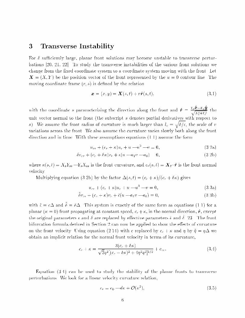
3 Transverse Instability

For � su�ciently large, planar front solutions may become unstable to transverse pertur-

bations [20, 21, 22]. To study the transverse instabilities of the various front solutions we

change from the �xed coordinate system to a coordinate system moving with the front. Let

X = (X;Y ) be the position vector of the front represented by the u = 0 contour line. The

moving coordinate frame (r; s) is de�ned by the relation

x = (x; y) =X(s; t) + rr(s; t); (3:1)

with the coordinate s parameterizing the direction along the front and r =

Y

s

x�X

s

y

p

X

2

s

+Y

2

s

the

unit vector normal to the front (the subscript s denotes partial derivatives with respect to

s). We assume the front radius of curvature is much larger than l

v

=

q

�=�, the scale of v

variations across the front. We also assume the curvature varies slowly both along the front

direction and in time. With these assumptions equations (1.1) assume the form

u

rr

+ (c

r

+ �)u

r

+ u� u

3

� v = 0; (3.2a)

�v

rr

+ (c

r

+ ��)v

r

+ �(u� a

1

v � a

0

) = 0; (3.2b)

where �(s; t) = X

s

Y

ss

�Y

s

X

ss

is the front curvature, and c

r

(s; t) =X

t

� r is the front normal

velocity.

Multiplying equation (3.2b) by the factor �(s; t) = (c

r

+ �)=(c

r

+ ��) gives

u

rr

+ (c

r

+ �)u

r

+ u� u

3

� v = 0; (3.3a)

~

�v

rr

+ (c

r

+ �)v

r

+ ~�(u� a

1

v � a

0

) = 0; (3.3b)

with ~� = �� and

~

� = ��. This system is exactly of the same form as equations (1.1) for a

planar (� = 0) front propagating at constant speed, c

r

+�, in the normal direction, r, except

the original parameters � and � are replaced by e�ective parameters ~� and

~

� [23]. The front

bifurcation formula derived in Section 2 can now be applied to show the e�ects of curvature

on the front velocity. Using equation (2.14) with c replaced by c

r

+ � and � by ~� = �� we

obtain an implicit relation for the normal front velocity in terms of its curvature,

c

r

+ � =

3(c

r

+ ��)

p

2q

2

[(c

r

+ ��)

2

+ 4�

2

q

2

]

1=2

+ c

1

: (3:4)

Equation (3.4) can be used to study the stability of the planar fronts to transverse

perturbations. We look for a linear velocity curvature relation,

c

r

= c

0

� d�+O(�

2

); (3:5)

6

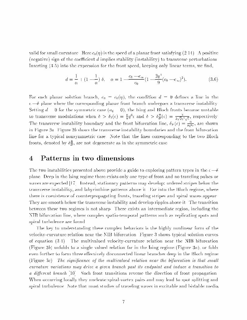
valid for small curvature. Here c

0

(�) is the speed of a planar front satisfying (2.14). A positive

(negative) sign of the coe�cient d implies stability (instability) to transverse perturbations.

Inserting (3.5) into the expression for the front speed, keeping only linear terms, we �nd,

d =

1

�

+ (1 �

1

�

) �; � = 1�

c

0

� c

1

c

0

(1�

2q

4

9

(c

0

� c

1

)

2

): (3:6)

For each planar solution branch, c

0

= c

0

(�), the condition d = 0 de�nes a line in the

�� � plane where the corresponding planar front branch undergoes a transverse instability.

Setting d = 0 for the symmetric case (a

0

= 0), the Ising and Bloch fronts become unstable

to transverse modulations when � > �

I

(�) =

8

9

q

6

� and � > �

�

B

(�) =

3

2

p

2q

3

p

�

, respectively.

The transverse instability boundary and the front bifurcation line, �

F

(�) =

9

8q

6

�

, are shown

in Figure 2a. Figure 2b shows the transverse instability boundaries and the front bifurcation

line for a typical nonsymmetric case. Note that the lines corresponding to the two Bloch

fronts, denoted by �

�

B

, are not degenerate as in the symmetric case.

4 Patterns in two dimensions

The two instabilities presented above provide a guide to exploring pattern types in the �� �

plane. Deep in the Ising regime there exists only one type of front and no traveling pulses or

waves are expected [17]. Instead, stationary patterns may develop: ordered stripes below the

transverse instability, and labyrinthine patterns above it. Far into the Bloch regime, where

there is coexistence of counterpropagating fronts, traveling stripes and spiral waves appear.

They are smooth below the transverse instability and develop ripples above it. The transition

between these two regimes is not sharp. There exists an intermediate region, including the

NIB bifurcation line, where complex spatio-temporal patterns such as replicating spots and

spiral turbulence are found.

The key to understanding these complex behaviors is the highly nonlinear form of the

velocity-curvature relation near the NIB bifurcation. Figure 3 shows typical solution curves

of equation (3.4). The multivalued velocity-curvature relation near the NIB bifurcation

(Figure 3b) unfolds to a single valued relation far in the Ising regime (Figure 3a), or folds

even further to form three e�ectively disconnected linear branches deep in the Bloch regime

(Figure 3c). The signi�cance of the multivalued relation near the bifurcation is that small

curvature variations may drive a given branch past its endpoint and induce a transition to

a di�erent branch [10]. Such front transitions reverse the direction of front propagation.

When occurring locally they nucleate spiral-vortex pairs and may lead to spot splitting and

spiral turbulence. Note that most studies of traveling waves in excitable and bistable media

7

[11, 12, 24] have assumed a linear relation, c

r

= c

0

� d�, which is valid only deep into the

Bloch regime (� � �

c

) and not near the NIB bifurcation (see also [25]).

4.1 Labyrinthine patterns

Far into the Ising regime and beyond the transverse instability line, � > �

I

(�) =

8

9

q

6

�, front

shapes meander, grow �ngers, and split at the tips. This behavior can be understood using

the velocity-curvature relation deep in the Ising regime, as depicted in Figure 4c. The positive

slope of this relation over a wide range of curvature implies that front portions with higher

curvature propagate faster, forming �ngers. It also implies that the transverse instability

remains e�ective even at the highly curved �ngertips. This leads to tip splitting.

Figure 5 shows the evolution of a stripe domain in the Ising regime above the transverse

instability boundary and corresponding to the velocity-curvature relation in Figure 4c. The

initial stripe is perturbed transversely along the middle part. The perturbation grows, forms

a meandering stripe, and then undergoes �ngering and tip splitting. A �nal stationary

labyrinth results when the pattern �lls the entire domain.

Notice the �nal pattern in Figure 5d is connected since there were no domain fusion

events during the evolution. Domain fusion is avoided by the repulsive front interactions

(due to the di�usive damping of v in the region between approaching fronts [17]). Closer to

the front bifurcation the front speeds are higher (see Figure 1b) and the repulsive interactions

may not be strong enough to prevent fusion. As a result the eventual stationary pattern

may contain disconnected domains.

Similar labyrinthine patterns have been observed in the bistable FIS reaction [5]. Our

interpretation is that these patterns occur in the Ising regime where the single front structure

corresponds to a high pH state invading a low pH state.

4.2 Single spot dynamics

Closer to the NIB bifurcation the nonlinearity of the velocity-curvature relation becomes

important. Consider an up state disk expanding radially outward. Depending on the system

parameters several scenarios for evolution are possible. Deep enough into the Ising regime,

where the velocity-curvature relation is still single valued (see Figure 4a), a stationary disk

solution exists. The disk has radius 1=�

0

, where c

r

(�

0

) = 0, and is stable to uniform

expansions and contractions because the velocity-curvature relation has positive slope at

c

r

= 0 (it might be unstable, however, to transverse perturbations [21]).

Still closer to the front bifurcation (but in the Ising regime) the velocity-curvature relation

becomes multivalued and the slope at c

r

= 0 negative as illustrated in Figure 4b. The

stationary disk is no longer stable to expansions and contractions and a breathing disk

solution appears [21]. To understand this breathing motion, note �rst that the boundary of

8

an expanding disk corresponds to a front lying on the upper branch in Figure 4b. As the

disk expands the front curvature decreases. When the curvature falls below the value where

the upper branch terminates a transition to the lower branch takes place. The disk stops

expanding and starts contracting. The curvature increases until the endpoint of the lower

branch is reached and a transition back to the upper branch occurs. As a result the disk

stops contracting and begins expanding again. These oscillations are similar to those found

in one-dimensional domains [17, 18, 26] with front interactions playing the role of curvature

in inducing front transitions [10].

To verify these expectations we studied numerically equations (1.1) in polar coordinates

assuming circularly symmetric front solutions (to avoid transverse instabilities). Such solu-

tions satisfy

u

t

= u

rr

+

1

r

u

r

+ u� u

3

� v; (4.1a)

v

t

= �v

rr

+

�

r

v

r

+ �(u� a

1

v � a

0

): (4.1b)

They represent circular fronts with curvatures �(t) = 1=r

0

(t), where r

0

(t) solves u(r

0

; t) = 0.

Figures 6a and 6b show the curvatures of up state disks as functions of time for parameters

pertaining to Figures 4a and 4b respectively. A single valued (multivalued) velocity-curvature

relation leads to a stationary (oscillatory) asymptotic state.

In fully two-dimensional systems oscillating disks might be unstable to non-circularly

symmetric perturbations. Consider an expanding disk perturbed to an oval shaped domain

as shown in Figure 7a. The parameters chosen pertain to a velocity-curvature similar to

the one in Figure 4b. As the domain expands the atter portions of its boundary are the

�rst to reach the end of the upper branch and undergo front transitions. These portions

then propagate towards one another, annihilate, and split the domain as shown in Figures

7b and 7c. The crossing points of the u = 0 and v = 0 contour lines indicate the cores

of spiral vortices. Note that the splitting process involves the creation and the subsequent

annihilation of two spiral-vortex pairs. A successive splitting is shown in Figure 7d. The

asymptotic state in this case is a disordered stationary pattern with many disconnected

domains. Remnants of the unstable breathing motion are often seen when the split spots

�rst contract, then approach a minimum size and start expanding. Both spot splitting and

the persistence of small spots have been observed recently be Lee et al. in the FIS reaction

[6] [27].

4.3 Spiral turbulence

Further approach to the NIB bifurcation results in disordered dynamic patterns where spiral

vortices nucleate and annihilate repeatedly. We refer to such a state as spiral turbulence. The

9

nucleation of spiral-vortex pairs results from local front transitions, very much like in spot

splitting except the mechanisms that drive the transitions are di�erent and depend on the

system parameters. For � su�ciently large, the transverse instability plays a dominant role in

inducing such transitions [28]. Figures 8 and 9 show spiral turbulence for smaller � values. In

this parameter regime front interactions are the major driving force. Figures 4f and 4g show

the corresponding velocity-curvature relations. In both �gures the upper branches terminate

at positive curvature values. Processes reducing the curvature of fronts on these branches

past the endpoints cause transitions to the lower front branches. As we have seen in the

previous section, single noncircularly symmetric domains may undergo such transitions and

split. In the presence of nearby domains, however, repulsive front interactions accelerate

domain splitting by attening out approaching curved fronts. Frames d; e; f of Figures 8

and 9 show local front transitions and splitting driven by front interactions (see the regions

indicated by the arrows). These processes are strikingly similar to those observed in the

FIS reaction [27]. Front interactions may also cause spiral-vortex nucleation and splitting by

directly inducing front transitions. Re ection of one-dimensional fronts provides an example

of front interactions leading to front transitions [17]. The spiral-vortex nucleations in Figures

8 and 9 are likely to result from both mechanisms.

The patterns in Figure 8 di�er from those in Figure 9 in a few respects. The initial

conditions in both simulations are the same but the subsequent spiral breakup is di�erent.

In Figure 8 most of the spiral wave disappears as the weakly curved front away from the core

undergoes a front transition. In Figure 9 the weakly curved part of the spiral survives longer

until front interactions or interactions with the boundaries come into play. This is because

the upper branch of the the velocity-curvature relation pertaining to Figure 9 terminates at

a lower curvature value than that of Figure 8 (see Figures 4f and 4g). Another di�erence

is the prevalence of more spots in the patterns of Figure 8. This is partly because domain

fusions are avoided in Figure 8 but occasionally take place in Figure 9 (closer to the NIB

bifurcation, front speeds are higher and domain fusions are more likely).

5 Numerical Methods

Numerical simulations were performed by integrating the system (1.1) with Neumann bound-

ary conditions. The spatial derivatives were computed by 4th order �nite di�erence approx-

imations on a uniform 400 � 400 grid over a domain of 0 � x � 400, 0 � y � 400. For

typical equation parameters the 400 � 400 resolution resulted in about 6 points across the

narrow front region in u. Doubling the resolution slightly changed the location of the front

bifurcation but did not a�ect the qualitative results. For the turbulent patterns (Figures 8

and 9) the time integration was performed with a second order Adams method. In the simu-

lations for the labyrinthine patterns and spot dynamics (Figures 5 and 7) the explicit Adams

10

method was replaced with an implicit second order formula for e�ciency of integration on

long time scales [29]. For the circularly symmetric simulations a one-dimensional version of

the 4th order �nite di�erence discretization was used with a variable order, variable step

size, implicit time integration scheme.

6 Conclusion

The Labyrinthine patterns found in the Ising regime have also been studied by Petrich and

Goldstein [30] using a nonlocal interface model. The model was derived for parameters far

into the Ising regime where the reaction-di�usion equations reduce to a gradient system. We

expect the qualitative predictions of this model to hold closer to the NIB bifurcation under

two conditions: domain fusion, which changes the topology of the front curve, does not take

place, and nongradient e�ects, such as front transitions, do not appear.

Spot splitting has been studied numerically by Pearson [31] and analytically, in one space

dimension, by Reynolds et al. [32]. No one-dimensional analog of spot splitting exists in the

present model, at least for the parameter regime where splitting in two dimensions has been

observed. The splitting studied here is a purely two-dimensional e�ect where curvature and

front interactions play key roles. We believe these factors also have important roles in the

two-dimensional spot splitting simulations by Pearson.

The breakup of spiral waves studied here results from local front transitions that become

feasible near the NIB bifurcation. The transitions can be induced by quite general pertur-

bations, either extrinsic or intrinsic. In [10] we studied front transitions caused by external

advective �elds. The transverse instability also can lead to local front transitions by creating

negatively curved front portions [28]. Here the important factors are front interactions that

act either directly, or indirectly (by attening curved fronts). It would be interesting to

investigate the relevance of the above mechanism to recent studies of spiral turbulence in

surface reactions [33] and in cardiac tissue models [34, 35, 36, 37, 38].

Many of the observations made here have also been found in the FIS reaction. These

include labyrinthine patterns [5], spot splitting [6], and front transitions induced by front

interactions [27]. Further comparative investigation should include experimental testing for

the existence of a NIB bifurcation, and examination of the experimental observations in

relation to the location of the bifurcation.

We expect similar complex spatio-temporal patterns to be found in other systems exhibit-

ing NIB bifurcations. Periodically forced oscillatory systems [8] and liquid crystals subjected

to rotating magnetic �elds might be good candidates [39, 40].

11

Acknowledgments

This work was supported in part by the Arizona Center for Mathematical Sciences (ACMS),

sponsored by AFOSR. One of us (A.H.) acknowledges the support of the Computational Sci-

ence Graduate Fellowship Program of the O�ce of Scienti�c Computing in the Department

of Energy.

12

References

[1] M. Seul, L. R. Monar, L. O'Gorman, and R. Wolfe, Science 254, 1616 (1991).

[2] R. E. Rosensweig, Ferrohydrodynamics (Cambridge University Press, Cambridge, U.

K., 1985).

[3] C. S. Henkee, E. L. Thomas, and L. J. Fetters, J. Mater. Sci. 23, 1685 (1988).

[4] T. A. Witten, Physics Today 43, 21 (1990).

[5] K. J. Lee, W. D. McCormick, Q. Ouyang, and H. L. Swinney, Science 261, 192 (1993).

[6] K. J. Lee, W. D. McCormick, H. L. Swinney, and J. E. Pearson, \Experimental ob-

servation of self-replicating spots in a reaction-di�usion system." Submitted to Nature

(unpublished).

[7] W. W. Mullins and R. F. Sekerka, J. Appl. Phys. 35, 444 (1964).

[8] P. Coullet, J. Lega, B. Houchmanzadeh, and J. Lajzerowicz, Phys. Rev. Lett. 65, 1352

(1990).

[9] A. Hagberg and E. Meron, Phys. Rev. E 48, 705 (1993).

[10] C. Elphick, A. Hagberg, and E. Meron, \Dynamic front transitions and spiral-vortex

nucleation." Submitted to Phys. Rev. Lett. (unpublished).

[11] E. Meron, Physics Reports 218, 1 (1992).

[12] J. J. Tyson and J. P. Keener, Physica D 32, 327 (1988).

[13] Y. A. Rzanov, H. Richardson, A. A. Hagberg, and J. V. Moloney, Physical Review A

47, 1480 (1993).

[14] B. S. Kerner and V. V. Osipov, Sov. Phys. Usp. 32, 101 (1989).

[15] T. Ohta and K. Kawasaki, Macromolecules 19, 2621 (1986).

[16] C. Roland and R. C. Desai, Phys. Rev. B 42, 6658 (1990).

[17] A. Hagberg and E. Meron, \Pattern formation in non-gradient reaction-di�usion sys-

tems: the e�ects of front bifurcations." To appear in Nonlinearity (unpublished).

[18] Y. Nishiura and M. Mimura, SIAM J. Appl. Math. 49, 481 (1989).

[19] J. Lajzerowicz and J. J. Niez, J. Phys. (Paris) Lett. 40, L185 (1979).

13

[20] D. A. Kessler and H. Levine, Phys. Rev. A 41, 5418 (1990).

[21] T. Ohta, M. Mimura, and R. Kobayashi, Physica D 34, 115 (1989).

[22] D. Horv�ath, V. Petrov, S. K. Scott, and K. Schowalter, J. Chem. Phys. 98, 6332 (1993).

[23] A. S. Mikhailov and V. S. Zykov, Physica D 52, 379 (1991).

[24] A. S. Mikhailov, V. A. Davydov, and V. S. Zykov, Physica D 70, 1 (1994).

[25] J. Sneyd and A. Atri, Physica D 65, 365 (1993).

[26] S. Koga and Y. Kuramoto, Prog. Theor. Phys. 63, 106 (1980).

[27] K. J. Lee, private communication.

[28] A. Hagberg and E. Meron, Phys. Rev. Lett. 72, 2494 (1994).

[29] C. W. Gear, Numerical Initial Value Problems in Ordinary Di�erential Equations (Pren-

tice Hall, Englewood Cli�s, NJ, 1985).

[30] D. M. Petrich and R. E. Goldstein, Phys. Rev. Lett. 72, 1120 (1994).

[31] J. E. Pearson, Science 261, 189 (1993).

[32] W. N. Reynolds, J. E. Pearson, and S. Ponce-Dawson, Phys. Rev. Lett. 72, 2797 (1994).

[33] M. B�ar and M. Eiswirth, Phys. Rev. E 48, R1635 (1993).

[34] M. Courtemanche and A. T. Winfree, Int. J. Bifurcation and Chaos 1, 431 (1991).

[35] A. V. Holden and A. V. Pan�lov, Int. J. Bifurcation and Chaos 1, 219 (1991).

[36] A. Karma, Phys. Rev. Lett. 71, 1103 (1993).

[37] M. Gerhardt, H. Schuster, and J. J. Tyson, Science 247, 1563 (1990).

[38] H. Ito and L. Glass, Phys. Rev. Lett. 66, 671 (1991).

[39] T. Frisch, S. Rica, P. Coullet, and J. M. Gilli, Phys. Rev. Lett. 72, 1471 (1994).

[40] K. B. Migler and R. B. Meyer, Physica D 71, 412 (1994).

14

Figure 1: The NIB front bifurcation in the (c; �) plane. The solid (broken) line represents

a stable (unstable) branch of front solutions. (top) The symmetric case, a

0

= 0. (bottom)

The nonsymmetric case, a

0

= �0:1.

1

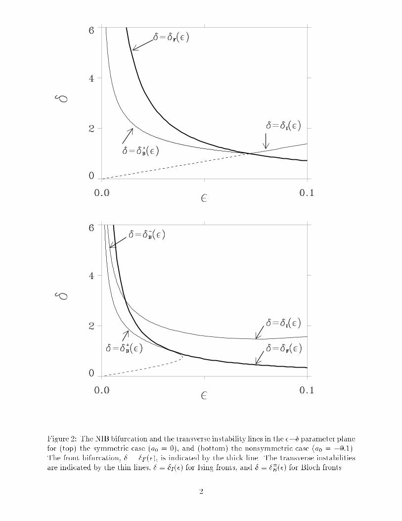
Figure 2: The NIB bifurcation and the transverse instability lines in the ��� parameter plane

for (top) the symmetric case (a

0

= 0), and (bottom) the nonsymmetric case (a

0

= �0:1).

The front bifurcation, � = �

F

(�), is indicated by the thick line. The transverse instabilities

are indicated by the thin lines, � = �

I

(�) for Ising fronts, and � = �

�

B

(�) for Bloch fronts.

2

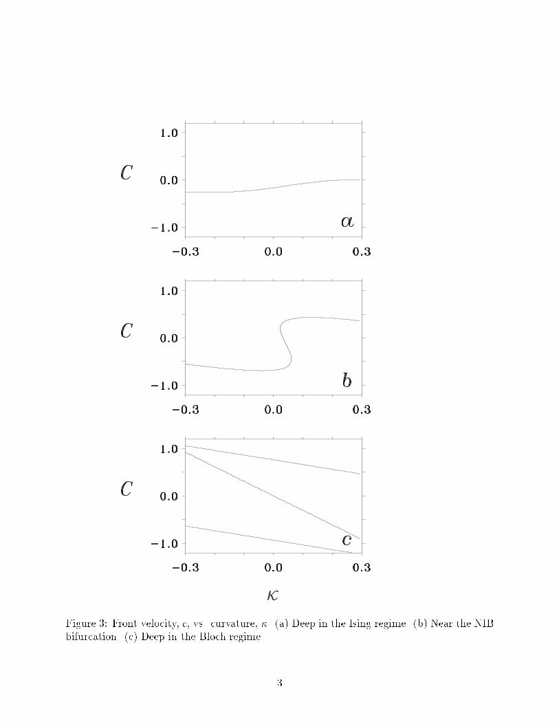
Figure 3: Front velocity, c, vs. curvature, �. (a) Deep in the Ising regime. (b) Near the NIB

bifurcation. (c) Deep in the Bloch regime.

3

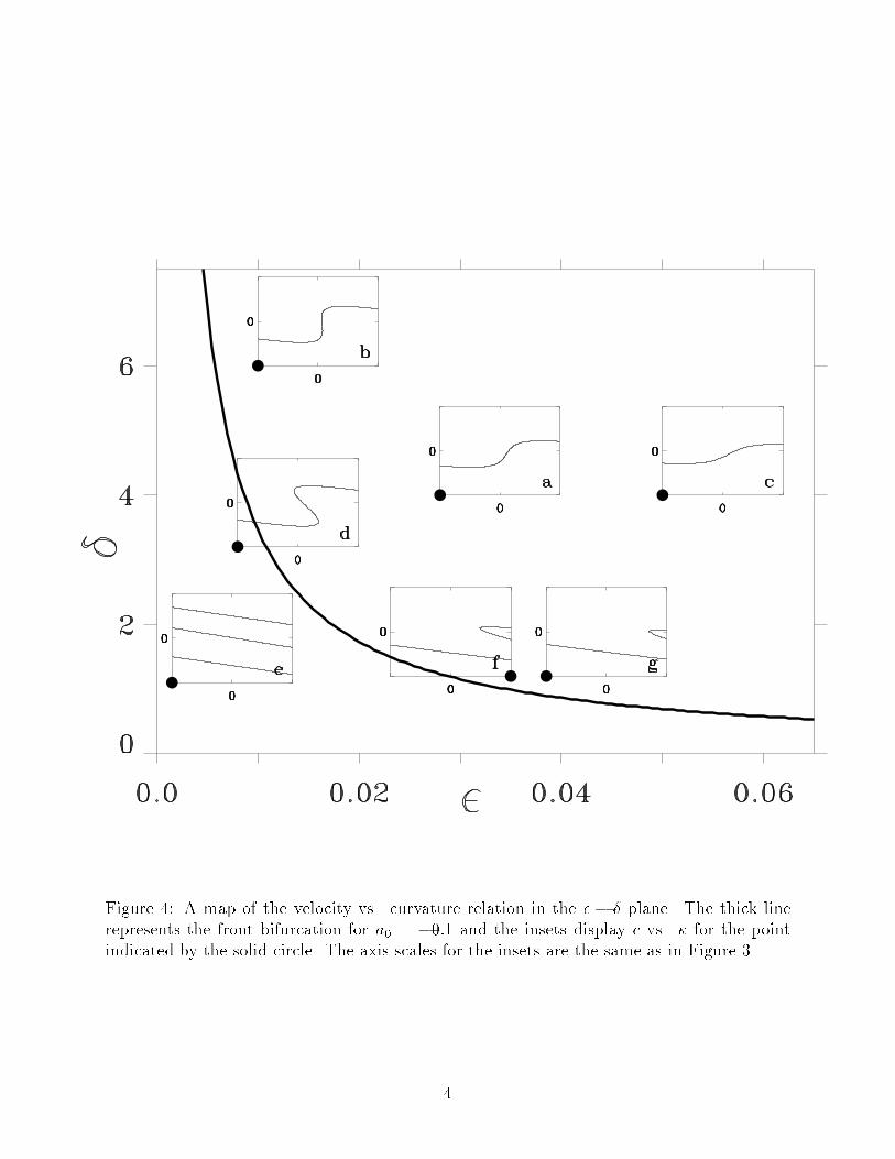
Figure 4: A map of the velocity vs. curvature relation in the � � � plane. The thick line

represents the front bifurcation for a

0

= �0:1 and the insets display c vs. � for the point

indicated by the solid circle. The axis scales for the insets are the same as in Figure 3.

4

Figure 5: The evolution of an initially perturbed stationary stripe in the Ising regime

above the transverse instability line (see Figure 4c). The dark and light regions corre-

spond to the up and down states respectively. The frames a; b; c; d; e; f pertain to times

t = 100; 525; 1100; 1900; 2675; 5000. The computational parameters are a

1

= 2:0, a

0

= �0:1,

� = 0:05, � = 4:0 on a domain of 0 � x � 400, 0 � y � 400.

5

Figure 6: Curvature, �, vs. time for a disk shaped domain. (top) Far in the Ising regime

(Figure 4a) a stationary disk pattern is reached. Computational parameters: a

1

= 2:0,

a

0

= �0:1, � = 0:028, � = 4:0. (bottom) Near the NIB bifurcation (Figure 4b) oscillations

set in. Computational parameters: a

1

= 2:0, a

0

= �0:1, � = 0:01, � = 6:0.

6

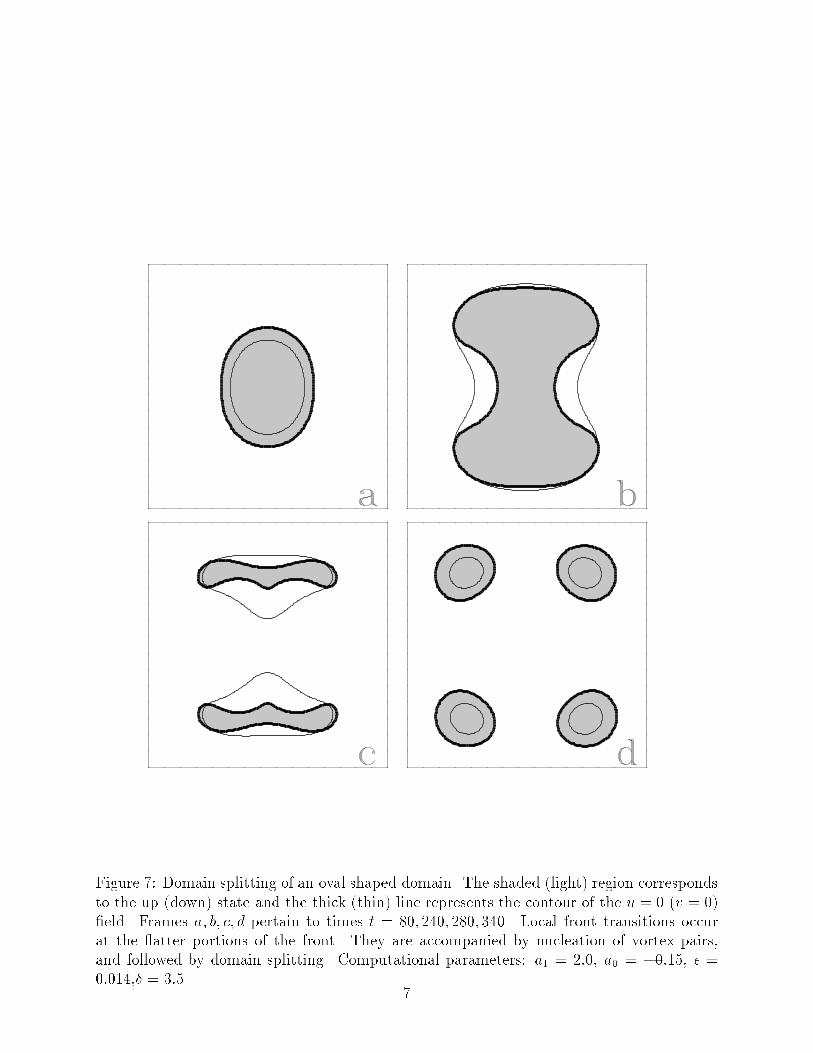
Figure 7: Domain splitting of an oval shaped domain. The shaded (light) region corresponds

to the up (down) state and the thick (thin) line represents the contour of the u = 0 (v = 0)

�eld. Frames a; b; c; d pertain to times t = 80; 240; 280; 340. Local front transitions occur

at the atter portions of the front. They are accompanied by nucleation of vortex pairs,

and followed by domain splitting. Computational parameters: a

1

= 2:0, a

0

= �0:15, � =

0:014,� = 3:5.

7

Figure 8: Spiral breakup for the velocity-curvature relation of Figure 4g. The frames

a; b; c; d; e; f represent the solution at times t = 60; 640; 1540; 3760; 3780; 3800 respectively.

The computational parameters are a

1

= 2:0, a

0

= �0:10, � = 0:0375, � = 1:2 on a domain

of 0 � x � 400, 0 � y � 400. For a more detailed description see the text.

8

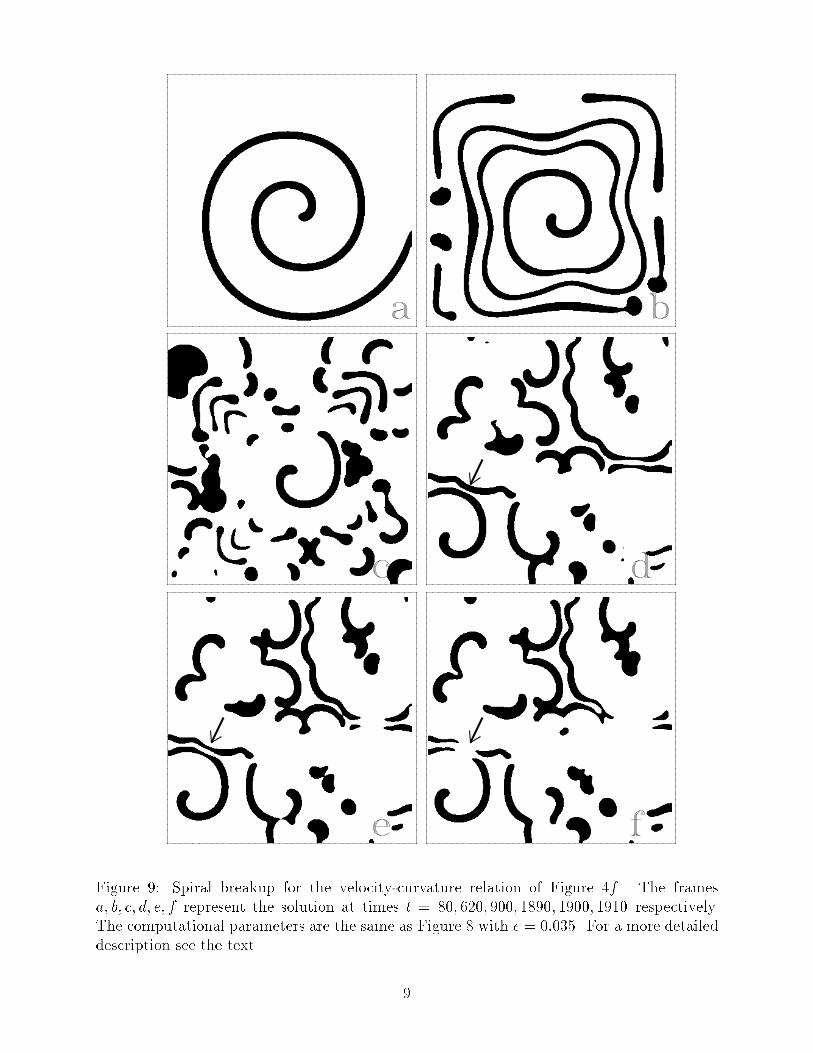
Figure 9: Spiral breakup for the velocity-curvature relation of Figure 4f . The frames

a; b; c; d; e; f represent the solution at times t = 80; 620; 900; 1890; 1900; 1910 respectively.

The computational parameters are the same as Figure 8 with � = 0:035. For a more detailed

description see the text.

9