The Stability and Dynamics of Localized Spot Patterns ... - arXiv

arX

iv:1

009.

2805

v1 [

nlin

.PS]

14

Sep

2010

Under consideration for publication in the SIAM Journal of Applied Dynamical Systems 1

The Stability and Dynamics of Localized Spot Patterns in

the Two-Dimensional Gray-Scott Model

W. CHEN, M. J. WARD

Wan Chen; Department of Mathematics, University of British Columbia, Vancouver, British Columbia, V6T 1Z2, Canada,(Currenntly at OCCAM, Oxford University, Oxford, U.K.)

Michael J. Ward; Department of Mathematics, University of British Columbia, Vancouver, British Columbia, V6T 1Z2, Canada(corresponding author)

(Received 10 September 2010)

The dynamics and stability of multi-spot patterns to the Gray-Scott (GS) reaction-diffusion model in a two-dimensional

domain is studied in the singularly perturbed limit of small diffusivity ε of one of the two solution components. A hybrid

asymptotic-numerical approach based on combining the method of matched asymptotic expansions with the detailed

numerical study of certain eigenvalue problems is used to predict the dynamical behavior and instability mechanisms of

multi-spot quasi-equilibrium patterns for the GS model in the limit ε → 0. For ε → 0, a quasi-equilibrium k-spot pattern

is constructed by representing each localized spot as a logarithmic singularity of unknown strength Sj for j = 1, . . . , k

at unknown spot locations xj ∈ Ω for j = 1, . . . , k. A formal asymptotic analysis is then used to derive a differential

algebraic ODE system for the collective coordinates Sj and xj for j = 1, . . . , k, which characterizes the slow dynamics of

a spot pattern. Instabilities of the multi-spot pattern due to the three distinct mechanisms of spot self-replication, spot

oscillation, and spot annihilation, are studied by first deriving certain associated eigenvalue problems by using singular

perturbation techniques. From a numerical computation of the spectrum of these eigenvalue problems, phase diagrams

representing in the GS parameter space corresponding to the onset of spot instabilities are obtained for various simple

spatial configurations of multi-spot patterns. In addition, it is shown that there is a wide parameter range where a spot

instability can be triggered only as a result of the intrinsic slow motion of the collection of spots. The construction of

the quasi-equilibrium multi-spot patterns and the numerical study of the spectrum of the eigenvalue problems relies

on certain detailed properties of the reduced-wave Green’s function. The hybrid asymptotic-numerical results for spot

dynamics and spot instabilities are validated from full numerical results computed from the GS model for various spatial

configurations of spots.

Key words: matched asymptotic expansions, spots, self-replication, logarithmic expansions, eigenvalues, Hopf bifur-cation, reduced-wave Green’s function, circulant matrix.

1 Introduction

Spatially localized spot patterns have been observed in a wide variety of experimental settings including, the

ferrocyanide-iodate-sulphite reaction (cf. [40]), the chloride-dioxide-malonic acid reaction (cf. [14]), and certain

electronic gas-discharge systems (cf. [3], [4]). Furthermore, numerical simulations of certain simple reaction-diffusion

systems, such as the two-component Gray-Scott model (cf. [48], [42]) and a three-component gas-discharge model

(cf. [52]), have shown the occurrence of complex spatio-temporal localized spot patterns exhibiting a wide range

of different instabilities including, spot oscillation, spot annihilation, and spot self-replication behavior. A survey of

experimental and theoretical studies, through reaction-diffusion (RD) modeling, of localized spot patterns in various

physical or chemical contexts is given in [55]. These experimental and numerical studies have provided considerable

impetus for developing a theoretical understanding of the dynamics, stability, and spot self-replication behavior asso-

ciated with localized solutions to singularly perturbed RD systems. A brief survey of some new directions and open

http://arxiv.org/abs/1009.2805v1

2 W. Chen, M. J. Ward

problems for the theoretical study of localized patterns in various applications is given in [30]. More generally, a wide

range of topics in the analysis of far-from-equilibrium patterns modeled by PDE systems are discussed in [45].

In this context, the goal of this paper is to provide a detailed case study of the dynamics, stability, and self-

replication behavior, of localized multi-spot patterns for the Gray-Scott (GS) RD system in a two-dimensional

domain. The GS model is formulated in dimensionless form as (cf. [44])

vt = ε2 ∆v − v +Auv2 , τut = D∆u+ (1− u)− uv2 , x ∈ Ω ∈ R2 ; ∂nu = ∂nv = 0 , x ∈ ∂Ω. (1.1)

Here ε > 0, D > 0, τ > 1, and A are constants. The parameter A is called the feed-rate parameter. For various ranges

of these parameters, (1.1) has a rich solution structure consisting of oscillating spots, spot annihilation behavior, spot

self-replication, and stripe and labyrinthian patterns. For the specific choice D = 2ε2, the complexity and diversity

of these patterns were first studied numerically in [48] in the unit square. Further numerical studies that clearly

exhibit the distinguishing phenomena of spot self-replication in a two-dimensional domain include [42] and [50].

For the study of localized patterns in the GS model (1.1), there are two distinguished limits for the diffusion

coefficient D in (1.1); the weak interaction regime with D = O(ε2), where the original numerical simulations of

the GS model were performed (cf. [48]), and the semi-strong interaction regime D = O(1), where many analytical

studies have been focused. In the weak interaction regime, there is only an exponentially weak coupling between any

two spots in the multi-spot pattern. This weak coupling arises from the exponential decay of a local spot profile. In

contrast, in the semi-strong interaction regime, and for a certain range of A, the spots are more strongly coupled

through the long-range effect of the slowly varying u component in (1.1). In this way, for D = O(1) the dynamics of

each individual spot in a multi-spot pattern is rather strongly influenced by the locations of the other spots in the

pattern, as well as by the geometry of the confining domain.

In a one-dimensional spatial domain, there has been much work over the past decade in analyzing the stability,

dynamics, and self-replication of spike patterns for the GS model (1.1). For the weak interaction regime where

D = O(ε2) and A = O(1), the mechanism for spike self-replication put forth in [46] (see also [54]) was based on

the occurrence of a nearly-coinciding hierarchical saddle-node global bifurcation structure for the global bifurcation

branches of multi-spike solutions. This mechanism was also shown to occur for the related Gierer-Meinhardt (GM)

system (cf. [45]). In this one-dimensional context, it was shown in [24] that typically only the spikes at the edges

of a multi-spike pattern can undergo splitting. The possibility of spatial-temporal chaotic behavior of spike patterns

due to repeated annihilation and self-replication events was explored in [47] from a global bifurcation viewpoint. The

study of solution behavior in this weak interaction regime relies heavily on the use of numerically computed global

bifurcation diagrams, since it appears to be analytically intractable to study the local problem near each spike. In

contrast, for the semi-strong interaction regime D = O(1) there are many analytical studies of spike behavior for

(1.1) for different ranges of the parameter A. For the range O(ε1/2) ≤ A≪ O(1), oscillatory instabilities of the spike

profile, characterized in terms of threshold values of the time-constant τ in (1.1), have been analyzed in [17], [18],

[43], [34], and [9]. Competition or annihilation instabilities of the spike profile, characterized by threshold values of

the diffusivity D, have been analyzed in [34] for the range A = O(ε1/2). In addition, self-replication instabilities of

spike patterns have been shown to occur only in the regime A = O(1), and they have been well-studied in [50], [51],

[18], [44], [35], and [20]. Weak translation, or drift, instabilities of spike patterns have been analyzed in [33] and

[35]. Finally, there have been several studies of the dynamical behavior of spike patterns for the one-dimensional GS

model including, two-spike dynamics for the infinite-line problem (cf. [15], [16]) and in a bounded domain (cf. [53]),

Localized Spot Patterns in the Two-Dimensional Gray-Scott Model 3

and multi-spike patterns on a bounded domain (cf. [9]). Related studies on the stability and dynamics of spike

solutions for the GM model in a one-dimensional domain are given in [29], [28], [59], [21], and [56] (see also the

references therein). For the semi-strong regime D = O(1), one key feature of the GS model (1.1) in one spatial

dimension is that the parameter regime A = O(ε1/2) where spike competition instabilities occur is well-separated in

parameter space from the range A = O(1) where spike self-replication occurs. As we discuss below, this feature with

the one-dimensional GS model is in distinct contrast to the two-dimensional GS model (1.1) where several distinct

spot instability mechanisms occur in nearby parameter regimes for A.

Although the stability properties of spike patterns for the one-dimensional case is rather well-understood, there

are only a few studies of the stability of multi-spot patterns for singularly perturbed two-component RD systems in

two dimensional domains. In particular, for the GS model (1.1) on the infinite plane Ω = R2, the existence and the

stability, with respect to locally radially symmetric perturbations, of a one-spot solution to (1.1) was studied in [60]

for the range A = O(ε(− ln ε)1/2) with either D = O(1) or D = O(ν−1), where ν ≡ −1/ ln ε . This rigorous study

was based on first deriving, and then analyzing, a certain nonlocal eigenvalue problem (NLEP). For the same range

of A, in [62] the one-spot NLEP stability analysis of [60] was extended to treat the case of multi-spot patterns on

a bounded domain. A further extension of this theory to study certain asymmetric multi-spot patterns was made

in [61]. The k-spot NLEP stability analysis of [62] for the regime A = O(ε(− ln ε)1/2) was based on retaining only

the leading-order term in powers of ν ≡ −1/ ln ε in the construction of the spot profile, and it pertains to the class

of locally radially symmetric perturbations near each spot. This theory characterizes competition and oscillatory

profile instabilities for the parameter range A = O(ε(− ln ε)1/2) with either D = O(1) or D = O(ν−1). In this

leading-order theory, the stability thresholds depend only on the number of spots, and not on their spatial locations

in the multi-spot pattern. Spot self-replication instabilities were not accounted for in these NLEP studies, as this

instability is triggered by a locally non-radially symmetric perturbation near each spot for the nearby parameter

regime A = O(ε(− ln ε)) (cf. [43]). A survey of NLEP stability theory as applied to other two-component singularly

perturbed RD systems, such as the GM and Schnakenburg models, is given in [63].

With regards to the dynamics of spots, there are only a few analytical results characterizing spot dynamics for

singularly perturbed RD systems in two-dimensional domains. These include, [11], [31] and [58] for a one-spot

solution of the GM model, [22], [23] and [25] for exponentially weakly interacting metastable spots in various

contexts, [38] for the Schnakenburg model, and [52] for a three-component gas-discharge RD model. We are not

aware of any previous study of the dynamics of spots for the GS model (1.1) in a two-dimensional domain.

We emphasize that the previous NLEP stability studies for the GS model (1.1) (cf. [60], [61], [62]) are based on

a leading-order theory in powers of ν = −1/ ln ε for the parameter range A = O(ε(− ln ε)1/2) with either D = O(1)

or D = O(ν−1). Therefore, since ν is not very small unless ε is extremely small, it is desirable to obtain a stability

theory for multi-spot solutions that accounts for all terms in powers of ν. However, more importantly, since the

scaling regime A = O(−ε ln ε) where a spot-replication instability can occur for (1.1) (cf. [43]) is logarithmically

close to the low feed-rate regime A = O(ε(− ln ε)1/2) studied in [62] and [60], where only competition or oscillatory

profile instabilities can occur, it is highly desirable to develop an asymptotic theory that incorporates these two

slightly different scaling regimes into a single parameter regime where all three types of spot instability can be

studied simultaneously. The leading-order theory in [62] is not sufficiently accurate to study the three types of spot

profile instability (competition, oscillatory, and self-replication) within a single parameter regime.

For the simpler Schnakenburg RD model, where competition and oscillatory instabilities do not occur when D =


O(1), a hybrid asymptotic-numerical method was developed in [38] to study the dynamics and self-replication

instabilities of a collection of spots for this specific RD model in an arbitrary two-dimensional domain. The theory,

which accounts for all terms in powers of ν = −1/ ln ε, was illustrated explicitly for the square and the disk, and the

results from this theory were favorably compared with full numerical computations of the RD system.

The main goal of this paper is to extend the theoretical framework of [38] for the Schnakenburg model to study

the dynamics and three types of instabilities associated with a collection of spots for the GS model (1.1) in the

semi-strong parameter regime D = O(1) with A = O(−ε ln ε). In our theory we account for all terms in powers of

ν = −1/ ln ε. In contrast to the Schnakenburg model of [38], we emphasize that there are three distinct instability

mechanisms for a collection of spots to the GS model (1.1) in this scaling regime for A and D that must be considered.

We now give an outline of the paper. In §2 and §3 the method of matched asymptotic expansions is used to construct

a quasi-equilibrium k-spot pattern for (1.1) that evolves slowly over a long O(ε−2) time scale. For this pattern, the

spatial profile for v concentrates at a set of points xj ∈ Ω for j = 1, . . . , k that drift with an asymptotically small

O(ε2) speed. Within an O(ε) neighborhood of each spot centered at xj , and at any instant in t, the local spot profiles

for u and v are radially symmetric to within O(ε) terms and satisfy a coupled system of BVP, referred to as the core

problem, on the (stretched) infinite plane. In the outer region, each spot at a given instant in time is represented

as a Coulomb singularity for u of strength Sj . The collective coordinates characterizing the slow dynamics of this

quasi-equilibrium k-spot pattern are the locations x1, . . . ,xk of the spots and their corresponding source strengths

S1, . . . , Sk, which measure the far-field logarithmic growth of the (inner) core solution for u near each spot. By

asymptotically matching the inner and outer solutions for u, we derive a differential algebraic system (DAE) of

ODE’s for the slow time evolution of these collective coordinates. At any instant in time, the quasi-equilibrium

solution is characterized as in Principal Result 2.1, where the source strengths Sj for j = 1, . . . , k are shown to

satisfy a coupled nonlinear algebraic system that depends on the instantaneous spot locations xj for j = 1, . . . , k,

together with certain properties of the reduced-wave Green’s function G(x;xj) and its regular part Rjj defined by

∆G− 1

DG = −δ(x− xj) , x ∈ Ω ; ∂nG = 0 , x ∈ ∂Ω , (1.2 a)

G(x;xj) ∼ − 1

2πln |x− xj |+Rj,j + o(1) , as x → xj . (1.2 b)

In Principal Result 3.1 of §3 the dynamical behavior of the collection of spots is characterized in terms of the source

strengths and certain gradients of the reduced-wave Green’s function. The overall DAE ODE system for xj and Sj ,

for j = 1, . . . , k, incorporates the interaction between the spots and the geometry of the domain, as mediated by

the reduced-wave Green’s function and its regular part, and it also accounts for all logarithmic correction terms in

powers of ν = −1/ ln ε in the asymptotic expansion of the solution. In this DAE ODE system there are two nonlinear

functions of Sj , defined in terms of the solution to the core problem, that must be computed numerically.

In §4.1 we study spot self-replication instabilities by first deriving a local eigenvalue problem near the jth spot that

characterizes any instability due to a non-radially symmetric local deformation of the spot profile. We emphasize that

in this stability analysis the local eigenvalue problems near each spot are not coupled together, except in the sense

that the source strengths S1, . . . , Sk must be determined from a globally coupled nonlinear algebraic system. The

spectrum of the local two-component linear eigenvalue problem near the jth spot is studied numerically, and we show

that there is a critical value Σ2 ≈ 4.31 of the source strength Sj for which there is a peanut-splitting linear instability

for any Sj > Σ2. These results for spot-splitting parallel those for the Schnakenburg model, as given in [38]. As a new

result, we derive and then numerically study a certain time-dependent elliptic-parabolic core problem near the jth


spot. Our computations from this time-dependent core problem strongly suggest that the localized peanut-splitting

linear instability of the quasi-equilibrium spot profile is in fact subcritical, and robustly triggers a nonlinear spot self-

replication event for the jth spot whenever Sj > Σ2. In summary, our hybrid asymptotic-numerical theory predicts

that if SJ > Σ2 ≈ 4.31 for some J ∈ 1, . . . , k then the Jth spot will undergo a nonlinear spot self-replication event.

Alternatively, the spots are all stable to self-replication whenever Sj < Σ2 for j = 1 . . . , k.

In §4.2 we use the method of matched asymptotic expansions to formulate a novel global eigenvalue problem

associated with competition or oscillatory instabilities in the spot amplitudes for a k-spot quasi-equilibrium solution

to (1.1) for the parameter range A = O(−ε ln ε) with D = O(1). This global eigenvalue problem, as formulated in

Principal Result 4.1, is associated with a locally radially symmetric perturbation near each spot, and it accounts

for all terms in powers of ν. It differs from the eigenvalue problem characterizing spot self-replication in that now

the local eigenfunction for the perturbation of the u component in (1.1) has a logarithmic growth away from the

center of each spot. This logarithmic growth leads to a global eigenvalue problem that effectively couples together

the local problems near each spot. A key component in the formulation of this global eigenvalue problem is a certain

eigenvalue-dependent Green’s matrix, with entries determined in terms of properties the Green’s function Gλ(x;xj)

satisfying ∆G−D−1(1 + τλ)G = −δ(x− xj) for x ∈ Ω, with ∂nG = 0 for x ∈ ∂Ω. This globally coupled eigenvalue

problem can be viewed, essentially, as an extended NLEP theory that accounts for all terms in powers of ν. In

§5–§6 we show that it determines thresholds for competition and oscillatory instabilities very accurately. However, in

contrast to the leading-order-in-ν NLEP stability studies (cf. [60], [62]) for A = O(

ε[− ln ε]1/2)

, our globally coupled

eigenvalue problem is not readily amenable to rigorous analysis. In Appendix B we briefly review the NLEP theory

of [60] and [62], and we show how our globally coupled eigenvalue problem can be reduced to leading order in ν to

the NLEP problems of [60] and [62] when A = O(

ε[− ln ε]1/2)

and D = O(ν−1).

In our stability analysis of §4 we linearize the GS model (1.1) around a quasi-equilibrium solution where the spots

are assumed to be at fixed locations x1, . . . ,xk, independent of time. However, since the spots locations undergo

a slow drift with speed O(ε2), the source strengths Sj for j = 1, . . . , k also vary slowly in time on a time-scale

t = O(ε−2). As a result of this slow drift, there can be triggered, or dynamically induced, instabilities of a quasi-

equilibrium spot pattern that is initially stable at time t = 0. To illustrate this, suppose that the pattern is initially

stable to spot self-replication at t = 0 in the sense that Sj < Σ2 at t = 0 for j = 1, . . . , k. Then, it is possible,

that as the Jth spot drifts toward its equilibrium location in the domain, that SJ > Σ2 after a sufficiently long

time of order t = O(ε−2). This will trigger a nonlinear spot self-replication event for the Jth spot. In a similar way,

we show that dynamically-triggered oscillatory and competition instabilities can also occur for a multi-spot pattern.

This dynamical bifurcation phenomena is similar to that for other ODE and PDE slow passage problems (cf. [5],

[39]) that have triggered instabilities generated by a slowly varying external bifurcation, or control, parameter. The

key difference here, is that the dynamically-triggered instabilities for the GS model (1.1) occur as a result of the

intrinsic motion of the collection of spots, and is not due to the tuning of an external control parameter.

In our numerical computations of competition and oscillatory instability thresholds from our globally coupled

eigenvalue problem of §4.2, we will for simplicity only consider k-spot quasi-equilibrium spot configurations x1, . . . ,xk

for which a certain Green’s matrix is circulant symmetric. For instance, this circulant matrix structure occurs when

k spots are equally spaced on a circular ring that is concentric within a circular disk, and it also occurs for other

spot patterns with sufficient spatial symmetry in other domains. Examples of such patterns are given in §5 and 6

below. Under this condition, we show in §2.1 that the source strengths Sj for j = 1, . . . , k have a common value. In


addition, by calculating the spectrum of the circulant symmetric Green’s matrix, we show in Principal Result 4.3 of

§4.3 that the globally coupled eigenvalue problem simplifies to k separate transcendental equations for the eigenvalue

parameter. In Appendix C we outline the numerical methods that we use to compute the instability thresholds from

the globally coupled eigenvalue problem under the circulant Green’s matrix assumption.

Spot patterns that give rise to this special circulant matrix structure are the direct counterpart of equally-spaced k-

spike patterns with spikes of a common amplitude, treated in almost all of the previous NLEP stability studies of the

GS and related RD models on a one-dimensional domain (cf. [17], [18], [34], [15], [16], [29], [59], [21], [56]). In one

spatial dimension, the only NLEP stability studies of an arbitrarily-spaced slowly evolving k-spike quasi-equilibrium

solution are the asymptotic-numerical study of dynamic competition instabilities for the Gierer-Meinhardt model

with τ = 0 in [28], and the study of oscillatory instabilities in [9] for the one-dimensional GS model for the range

O(ε1/2) ≪ A≪ O(1). For this range of A it was shown in [9] that the k separate NLEP problems can be reduced, via

a scaling law, to only one single NLEP problem. To date, there has been no NLEP stability study of a slowly evolving

arbitrarily-spaced k-spike quasi-equilibrium spike pattern in a one-dimensional domain that takes into account both

competition and oscillatory instabilities. As a result, in our two-dimensional setting, it is a natural first step to study

the global eigenvalue problem, which governs competition and oscillatory instabilities, under the circulant matrix

condition, which allows for spots of a common source strength.

In §5 the asymptotic theory of §2– §4 is illustrated for the case of both one and two-spot quasi-equilibrium solutions

to the GS model (1.1) on the infinite plane. Phase diagrams characterizing the GS parameter ranges for the different

types of instabilities are derived for these simple spot patterns. In particular, for two spots that are sufficiently

far apart, we show that spot self-replication instabilities will occur when A exceeds some threshold. In contrast, a

competition instability will occur if the two spots are too closely spaced. For a very large, but finite, domain the full

numerical simulations in §5.3 are used to validate the stability results from the asymptotic theory.

In §6 the asymptotic theory of §2– §4 is implemented and compared with full numerical results computed from

(1.1) for various special multi-spot patterns on the unit disk and square for which a certain Green’s matrix has

a circulant matrix structure. For these domains, the explicit formulae for the reduced-wave Green’s function and

its regular part, as derived in Appendix A, are used to numerically implement the asymptotic theory. The overall

hybrid asymptotic-numerical approach provides phase diagrams in parameter space characterizing both the stability

thresholds and the possibility of dynamically-triggered instabilities. One key theoretical advantage of considering the

unit disk is that the reduced-wave Green’s function can be well-approximated for D ≫ 1 by the Neumann Green’s

function, which has a simple explicit formula in the unit disk. By using this explicit formula, the hybrid asymptotic-

numerical framework of §2– §4 can be studied, to a large extent, analytically for the case of k equally-spaced spots

on a ring that is concentric within the unit disk.

In §7 we compare our theoretical predictions for spot dynamics and spot self-replication instabilities with full

numerical results computed from (1.1) for a few simple “asymmetric” spot patterns for which the associated Green’s

matrix is not circulant. We show that the dynamics in Principal Result 3.1 accurately determines spot dynamics before

a self-replication event, and with a re-calibration of the initial spot locations, it accurately predict spot dynamics

after a spot-splitting event. We emphasize that since the local eigenvalue problems near each spot are decoupled for

the case of locally non-radially symmetric perturbations, the onset of spot self-replication behavior only depends on

the source strength of an individual spot. Therefore, given any initial spatial configuration of spots at t = 0, we need

only solve the nonlinear algebraic system for Sj , j = 1, · · · , k at t = 0 to predict that the jth spot undergoes splitting


starting at t = 0 when Sj > Σ2 ≈ 4.31. A special asymmetric pattern that we consider in some detail in §7 is a

k-spot pattern consisting of k − 1 equally-spaced spots on a ring concentric within the unit disk, with an additional

spot at the center of the unit disk. For D ≫ 1, we use the simple explicit formula for the Neumann Green’s function

to explicitly predict the occurrence of dynamically-triggered spot self-replication instabilities for this special pattern.

Although the hybrid asymptotic-numerical framework developed herein to study the stability and dynamics of

multi-spot quasi-equilibrium patterns for the GS model (1.1) is related to that initiated for the Schnakenburg model

in [38], there are some key differences in the analysis and in the results obtained. The primary difference between

these two models is that the GS model (1.1) admits three types of instability mechanisms, whereas only spot self-

replication instabilities can occur for the Schnakenburg model of [38] when D = O(1). In addition, in contrast to

our study in §5 of one- and two-spot patterns to the GS model on the infinite plane, the Schnakenburg model of [38]

is ill-posed in R2. Finally, our results for the GS model (1.1) show that there is a wide parameter range and many

simple spot configurations for which we can theoretically predict the occurrence of dynamically-triggered instabilities

due to either competition, oscillation, or splitting. These dynamically-triggered bifurcation events can occur even

within the very simple context of a multi-spot pattern with a common source strength. For these special patterns,

such instabilities cannot occur for the Schnakenburg model.

Finally, although this paper focuses only on the study of spot patterns, we remark that the GS model (1.1) supports

patterns of increasing complexity as the feed-rate parameter A increases. In particular, in the range O(ε1/2) ≪ A≪O(1), the GS model (1.1) with D = O(1) on a two-dimensional domain does not admit spots, but instead allows

for solutions for which v concentrates on a higher dimensional set such as on a one-dimensional stripe or a one-

dimensional ring inside a two-dimensional domain. A stability analysis of a planar stripe inside a square domain or

a concentric ring inside a disk was given in [41] and in [37].

2 K-Spot Quasi-Equilibrium Solutions

We first construct a k-spot quasi-equilibrium solution to (1.1) by using the method of matched asymptotic expansions.

We denote the center of the jth spot by xj = (xj , yj) ∈ Ω for j = 1, . . . , k. We assume that the spots are well-separated

in the sense that |xi − xj | = O(1) for i 6= j, and dist(xj , ∂Ω) = O(1) for j = 1, . . . , k. In an O(ε) neighborhood near

the jth spot, we get v = O(ε−1) and u = O(ε). Thus, we introduce the local variables Uj , Vj , and y, defined by

u =ε

A√DUj , v =

√D

εVj , y = ε−1(x − xj) . (2.1)

In terms of these local variables, (1.1) transforms to

∆yVj − Vj + UjV2j = 0 , ∆yUj − UjV

2j +

εA√D

− ε2

DUj = 0 , y ∈ R

2 . (2.2)

We look for a radially symmetric solution to (2.2) of the form Uj = Uj(ρ) and Vj = Vj(ρ), where ρ ≡ |y|. Then, toleading order in ε, Uj and Vj are the solutions to the radially symmetric problem

U ′′j +

1

ρU ′j − UjV

2j = 0 , V ′′

j +1

ρV ′j − Vj + UjV

2j = 0 , 0 < ρ <∞ , (2.3 a)

V ′j (0) = 0 , U ′

j(0) = 0 ; Vj(ρ) → 0 , Uj(ρ) ∼ Sj ln ρ+ χ(Sj) + o(1) , as ρ→ ∞ . (2.3 b)

This leading-order coupled inner problem is referred to as the core problem, and is the same as that derived in [38]

for the Schnakenburg model. We refer to Sj as the source strength of the jth spot. From the divergence theorem, it


follows from the Uj equation in (2.3) that Sj =∫∞0 UjV

2j ρ dρ > 0. In the far-field behavior (2.3 b) for Uj, the constant

χ is a nonlinear function of the source strength Sj, which must be computed numerically from the solution to (2.3).

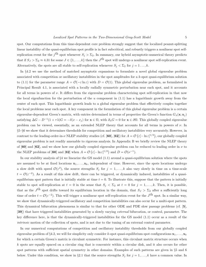
The solution to (2.3) is calculated numerically for a range of values of Sj > 0 by using the BVP solver COLSYS

(cf. [2]). In Fig. 1, we plot χ(Sj), Vj(0) versus Sj , and Vj(ρ) for a few different values of Sj . For Sj > Sv ≈ 4.78,

the profile Vj(ρ) has a volcano shape, whereby the maximum of Vj occurs at some ρ > 0. These computations give

numerical evidence to support the conjecture that there is a unique solution to (2.3) for each Sj > 0.

1 2 3 4 5 6 7

−5

0

5

10

15

20

Sj

χ

(a) χ vs. Sj

0 2 4 6 80

0.1

0.2

0.3

0.4

0.5

0.6

0.7

0.8

Sj

Vj(0

)

(b) Vj(0) vs. Sj

0 5 10 150

0.1

0.2

0.3

0.4

0.5

0.6

0.7

0.8

ρ

Vj

(c) Vj vs. ρ

Figure 1. Numerical results for the core problem (2.3) (a) The function χ vs. Sj; (b) Vj(0) vs. Sj; (c) The spot profile

Vj(ρ) for Sj = 0.94, 1.45, 2.79 (solid curves where Vj(0) is the maximum of Vj(ρ)), and the volcano profile Vj(ρ) for

Sj = 4.79, 5.73, 6.29 (the dotted curves correspond to cases where the maximum of Vj(ρ) occurs for ρ > 0).

Since v is localized near each xj for j = 1, . . . , k, and is exponentially small in the outer region away from the spot

centers, the effect of the nonlinear term uv2 in the outer region can be calculated in the sense of distributions as

uv2 ∼ ε2∑k

j=1

(

∫

R2

√D (Aε)

−1UjV

2j dy

)

δ(x−xj) ∼ 2πε√DA−1

∑kj=1 Sj δ(x−xj). Therefore, in the quasi-steady

limit, the outer problem for u from (1.1) is

D∆u + (1− u) =2π

√D ε

A

k∑

j=1

Sj δ(x− xj) , x ∈ Ω ; ∂nu = 0 , x ∈ ∂Ω , (2.4 a)

u ∼ ε

A√D

(

Sj ln |x− xj | − Sj ln ε+ χ(Sj))

, as x → xj , j = 1, . . . , k . (2.4 b)

The singularity condition (2.4 b) for u as x → xj was derived by matching the outer solution for u to the far-field

behavior (2.3 b) of the core solution, and by recalling u = εUj/(A√D) from (2.1). The problem (2.4) suggests that

we introduce new variables A = O(1) and ν ≪ 1 defined by

ν = −1/ ln ε , A = νA√D/ε = A

√D/ [−ε ln ε] . (2.5)

In terms of these new variables, (2.4) transforms to

∆u+(1 − u)

D=

2πν

A

k∑

j=1

Sj δ(x − xj) , x ∈ Ω ; ∂nu = 0 , x ∈ ∂Ω , (2.6 a)

u ∼ 1

A [Sjν ln |x− xj |+ Sj + νχ(Sj)] , as x → xj , j = 1, . . . , k . (2.6 b)

We emphasize that the singularity behavior in (2.6 b) specifies both the strength of the logarithmic singularity for u

and the regular, or non-singular, part of this behavior. This pre-specification of the regular part of this singularity

behavior at each xj will yield a nonlinear algebraic system for the source strengths S1, . . . , Sk.


The solution to (2.6) is represented as u = 1−∑k

i=1 2πνA−1SiG(x;xi), where G(x;xi) is the reduced-wave Green’s

function defined by (1.2). By expanding u as x → xj , and then equating the resulting expression with the required

singularity behavior in (2.6 b), we obtain the following nonlinear algebraic system for S1, . . . , Sk:

A = Sj(1 + 2πνRj,j) + νχ(Sj) + 2πν

k∑

i=1

i6=j

SiG(xj ;xi) , j = 1, . . . , k . (2.7)

Given the GS parameters A, ε and D, we first calculate A and ν from (2.5), and then solve (2.7) numerically for the

source strengths S1, . . . , Sk. With Sj known, the quasi-equilibrium solution in each inner region is determined from

(2.3). As a remark, since A = O(1), then A = O(−ε ln ε) from (2.5). Therefore, the error made in approximating

(2.2) by (2.3) in the inner region is of the order O(−ε2 ln ε). We summarize our result as follows:

Principal Result 2.1: For ε → 0 assume that A = O(−ε ln ε), and define ν and A by ν = −1/ ln ε and A =

νA√D/ε, where A = O(1). Then, the solution v and the outer solution for u, corresponding to a k-spot quasi-

equilibrium solution of the GS model (1.1), are given asymptotically by

u(x) ∼ 1− 2πν

A

k∑

j=1

SjG(x;xj) , v(x) ∼√D

ε

k∑

j=1

Vj(

ε−1|x− xj |)

. (2.8 a)

Moreover, the inner solution for u, defined in an O(ε) neighborhood of the jth spot, is

u(x) ∼ ν

AUj

(

ε−1|x− xj |)

. (2.8 b)

Here x1, . . . ,xk is the spatial configuration of the centers of the spots, and G(x;xj) is the reduced-wave Green’s

function satisfying (1.2). In (2.8), each spot profile Vj(ρ) and Uj(ρ) for j = 1, . . . , k satisfies the coupled BVP system

(2.3), where the source strength Sj in (2.3 b) is to be calculated from the nonlinear algebraic system (2.7).

We emphasize that the nonlinear algebraic system (2.7) determines the source strengths Sj for j = 1, . . . , k to

within an error smaller than any power of ν = −1/ ln ε. As such, our construction of the quasi-equilibrium pattern

is accurate to all orders in ν. Similar techniques for summing logarithmic expansions in the context of linear elliptic

PDE’s or eigenvalue problems in two-dimensional perforated domains containing small holes have been developed

in a variety of contexts (cf. [57], [32], [13], [49]). Our construction here of a quasi-equilibrium solution for the GS

model (1.1) extends this previous methodology for treating logarithmic expansions to an RD system for which the

local problem is nonlinear with a logarithmic far-field behavior. The nonlinear algebraic system (2.7) for the source

strengths is the mechanism through which the spots interact and sense the presence of the domain Ω. This global

coupling mechanism, which is not of nearest-neighbor type as in the case of the exponentially weak spot interactions

studied in [23] and [25], is rather significant since ν = −1/ ln ε is not very small unless ε is extremely small.

The quasi-equilibrium solution in Principal Result 2.1 exists only when the spatial configuration of spots and the

GS parameters are such that the nonlinear algebraic system (2.7) for S1, . . . , Sk has a solution. Determining precise

conditions for the solvability of this system is a difficult issue. Therefore, in §5–7 we will primarily consider spot

patterns where the source strengths have a common value, for which (2.7) reduces to a scalar nonlinear equation.

Next, we derive analytical approximations for the solution to (2.7) by first re-writing (2.7) in matrix form. To do


so, we define the Green’s matrix G, the vector of source strengths s, the vector χ(s), and the identity vector e by

G ≡

R1,1 G1,2 · · · G1,k

G2,1. . .

. . ....

.... . .

. . . Gk−1,k

Gk,1 · · · Gk,k−1 Rk,k

, s ≡

S1

...

Sk

, e ≡

1...

1

, χ(s) ≡

χ(S1)...

χ(Sk)

. (2.9)

Here Gi,j ≡ G(xi;xj), and Gi,j = Gj,i by reciprocity, so that G is a symmetric matrix. Then, (2.7) becomes

A e = s+ 2πνG s+ νχ(s) . (2.10)

We will consider (2.10) for two ranges of D; D = O(1) and D = O(ν−1). For D = O(1), we can obtain a two-term

approximation for the source strengths in terms of ν ≪ 1 by expanding s = s0 + νs1 + · · · . This readily yields

s = Ae− ν [2πAG e+ χ(A)e] +O(ν2) . (2.11)

Therefore, for ν ≪ 1, the leading-order approximation for s is the same for all of the spots. However, the O(ν)

correction term depends on the spot locations and the domain geometry.

Next, we consider (2.10) for the distinguished limit where D = D0/ν ≫ 1 with D0 = O(1). Since the reduced-wave

Green’s function G, satisfying (1.2), depends on D we first must approximate it for D large. Assuming that Ω is a

bounded domain, we expand G and its regular part R for D ≫ 1 as

G ∼ DG−1 +G0 +1

DG1 + · · · , R ∼ DR−1 +R0 +

1

DR1 + · · · .

Substituting this expansion into (1.2), and collecting powers of D, we obtain that G−1 is constant and that

∆G0 = G−1 − δ(x − xj) , x ∈ Ω ; ∂nG0 = 0 , x ∈ ∂Ω .

The divergence theorem then shows that G−1 = |Ω|−1, where |Ω| is the area of Ω. In addition, the divergence theorem

imposed on the G1 problem enforces that∫

ΩG0 dx = 0, which makes G0 unique. Next, from the singularity condition

(1.2 b) for G we obtain for x → xj that DG−1 + G0(x;xj) + · · · ∼ −(2π)−1 ln |x − xj | + DR−1 + R0(x;xj) + · · · .Since G−1 = |Ω|−1, we conclude that R−1 = G−1 = 1/|Ω|. In this way, we obtain the following two-term expansion

Rj,j ∼ Rj,j ≡D

|Ω| +R(N)j,j + · · · , G(x;xj) ∼ G(x;xj) ≡

D

|Ω| +G(N)(x;xj) + · · · , for D ≫ 1 . (2.12)

Here G(N)(x;xj) is the Neumann Green’s function with regular part R(N)j,j , determined from the unique solution to

∆G(N) =1

|Ω| − δ(x− xj) , x ∈ Ω ; ∂nG(N) = 0 , x ∈ ∂Ω ;

∫

Ω

G(N) dx = 0 , (2.13 a)

G(N)(x;xj) ∼ − 1

2πln |x− xj |+R

(N)j,j + o(1) , as x → xj . (2.13 b)

For the disk and the square, in Appendix A we analytically calculate both G(x;xj) and its regular part Rj,j , as

well as the Neumann Green’s function G(N)(x;xj) and its regular part R(N)j,j . For the case of a one-spot solution

centered at the midpoint x1 of the unit square [0, 1]× [0, 1], we use some of the explicit formulae from Appendix A

to compare the two-term approximation R1,1, given in (2.12), with the reduced-wave regular part R1,1, as computed

from (A.11). These results are shown in Fig. 2. From (A.13), the two-term approximation (2.12) for large D is

R1,1 = D − 1

π

∞∑

n=1

ln (1− qn) +1

12− 1

2πln(2π) , q ≡ e−2π . (2.14)


A similar comparison is made in Fig. 3 for the case of a single spot located at the center x1 = (0, 0) of the unit disk.

For this radially symmetric case R1,1 can be found explicitly, and its two-term approximation for large D is obtained

from (2.12) and (A.9 b). In this way, we get

R1,1 =1

2π

[

1

2lnD + ln 2− γe +

K1

(

D−1/2)

I1(

D−1/2)

]

, R1.1 =D

π− 3

8π. (2.15)

Here γe ≈ 0.5772 is Euler’s constant, while I1(r) and K1(r) are the modified Bessel functions of order one. From

Fig. 2 and Fig. 3 we observe that for both domains the two-term approximation (2.12) involving the regular part of

the Neumann Green’s provides a decent approximation of R1,1 even for only moderately large values of D.

0 1 2 3 4 5 6−1

0

1

2

3

4

5

6

D

R1,

1

(a) R1,1 and R1,1 vs. D

0.1 0.2 0.3 0.4 0.5

−0.1

0

0.1

0.2

0.3

0.4

D

R1,

1

(b) R1,1 and R1,1 vs. D

Figure 2. Consider a single spot centered at the midpoint x1 = (0.5, 0.5) of the unit square. We plot R1,1 vs. D (solid

curve) and its two-term large D approximation R1,1 given in (2.14) (dotted curve). (a) D ∈ [0.1, 6]; (b) D ∈ [0.1, 0.5].

0 1 2 3 4 5 6−0.5

0

0.5

1

1.5

2

D

R1,

1

(a) R1,1 and R1,1 vs. D

0.1 0.2 0.3 0.4 0.5

−0.1

−0.05

0

0.05

0.1

D

R1,

1

(b) R1,1 and R1,1 vs. D

Figure 3. Consider a single spot located at the center x1 = (0, 0) of the unit disk. We plot R1,1 vs. D given in

(2.15) (dotted curve) and its two-term large D approximation R1.1 given in (2.15) (solid curve). (a) D ∈ [0.1, 6]; (b)

D ∈ [0.1, 0.5].

Next, we use the large D asymptotics to find an approximate solution to the nonlinear algebraic system (2.10) in

the limit D = D0/ν ≫ 1, where D0 = O(1) and ν ≪ 1. Upon substituting (2.12) into (2.10) we obtain

Ae = s+2πD0

|Ω| e eT s+ 2πνG(N)s+ νχ(s) ,

where G(N) is the Green’s matrix associated with the Neumann Green’s function, i.e. G(N)i,j = G(N)(xi;xj) for i 6= j,


and G(N)j,j ≡ R

(N)j,j . By expanding s as s = s0 + νs1 + · · · for ν ≪ 1, we then obtain that s0 and s1 satisfy

(

I +2πD0

|Ω| eeT)

s0 = Ae ,

(

I +2πD0

|Ω| eeT)

s1 = −2πG(N)s0 − χ(s0) , (2.16)

where I is the k × k identity matrix. Since eT e = k, the leading-order approximation s0 shows that the source

strengths have an asymptotically common value Sc given by

s0 = Sce , Sc ≡A

1 + µk, µ ≡ 2πD0

|Ω| . (2.17)

The next order approximation s1 from (2.16) yields

s1 = −(

I + µeeT)−1

(

2πScG(N) + χ(Sc))

e . (2.18)

Since the matrix I + µeeT is a rank-one perturbation of the identity, its inverse is readily calculated from the

Shermann-Woodbury-Morrison formula as (I + µeeT )−1 = I − µeeT /(1 + µk), which determines s1 from (2.18). In

this way, for D = D0/ν and ν ≪ 1 we obtain the two-term expansion for s given by

s = Sce−(

χ(Sc)

1 + µke+

2πA1 + µk

(

G(N) − µF

1 + µkI)

e

)

ν +O(ν2) . (2.19)

Here Sc and µ are defined in (2.17), while the scalar function F (x1, . . . ,xk) is defined by

F (x1, . . . ,xk) = eTG(N) e =k∑

i=1

k∑

j=1

G(N)i,j . (2.20)

In contrast to the leading-order approximation in (2.11) when D = O(1), the leading-order approximation Sc in

(2.19) depends on the number of spots and the area of the domain, with Sc increasing as the area |Ω| increases.We now illustrate our asymptotic theory for the construction of quasi-equilibria for the case of a one-spot solution

centered at the midpoint of either the unit square or disk. Many additional examples of the theory are given in §5–6.For our first example, we consider a one-spot solution with a spot located at the center x1 = 0 of the unit disk with

ε = 0.02. We fix D = 1, so that from (2.15) the regular part of the Green’s function for a spot at x1 is R1,1 ≈ 0.1890.

Then, (2.7) reduces to the following scalar nonlinear algebraic equation for the source strength S1 in terms of A:

A = S1 (1 + 2πνR1,1) + νχ(S1) . (2.21)

In Fig. 4(a) we plot A versus S1, showing the existence of a fold point at Af ≈ 2.55 corresponding to Sf ≈ 1.01.

Thus, A ≥ Af is required for the existence of a one-spot quasi-equilibrium solution located at the center of the unit

disk. In Fig. 4(b) the asymptotic result for u(x1) = ν U1(0)/A vs. A is shown by the dotted curve, with a fold point at

uf (x1) ≈ 0.50. The fold point is marked by a circle in both figures, and the critical value Av ≈ 5.55, uv(x1) ≈ 0.083

for a volcano-type solution corresponding to Sv ≈ 4.78 is marked by a square. For A > Af , u(x1) has two solution

branches. The upper branch corresponds to S1 < Sf , while the lower branch is for the range S1 > Sf .

To validate the asymptotic result for solution multiplicity, we solve the steady-state GS model (1.1) in the unit

disk by using the Matlab BVP solver BVP4C. By varying u(0), we then compute the corresponding value of A. The

resulting full numerical result for u(0) vs. A is shown by the heavy solid curve in Fig.4(b), which essentially overlaps

the asymptotic result. This shows that when ε = 0.02, the asymptotic result for the bifurcation diagram, based on

retaining all terms in powers of ν, agrees very closely with the full numerical result.

For our second example, we consider a one-spot solution centered at the midpoint x1 = (0.5, 0.5) of the unit square

Ω = [0, 1]× [0, 1]. We fix ε = 0.02 and D = 1. Then, by using (A.11) for the reduced-wave Green’s function, as given


3

4

5

6

7

0 1 2 3 4 5 6 7 8

A

S1

(a) A vs. S1

00.10.20.30.40.50.60.70.8

0.91.0

3 4 5 6 7

u(x 1)

A

(b) u(x1) vs. A

Figure 4. Let Ω = x||x| ≤ 1, ε = 0.02, D = 1, and x1 = 0. (a) A vs. S1; the square marks the volcano threshold

Sv ≈ 4.78, and the circle marks the fold point Af ≈ 2.55 at which Sf ≈ 1.01. (b) u(x1) vs. A; the square marks

Sv ≈ 4.78, and the circle marks the fold point Sf ≈ 1.01. The upper branch is for S1 < Sf , and the lower branch is

for S1 > Sf .

2

4

6

8

10

12

14

16

0 1 2 3 4 5 6 7 8

A

S1

(a) A vs. S1

00.10.20.30.40.50.60.70.8

0.91.0

2 4 6 8 10 12 14 16

u(x 1)

A

(b) u(x1) vs. A

Figure 5. Let Ω = [0, 1] × [0, 1], ε = 0.02, D = 1, and x1 = (0.5, 0.5). (a) A vs. S1; the square marks the volcano

threshold Sv ≈ 4.78, and the circle marks the fold point Af ≈ 3.3756 at which Sf ≈ 0.7499. (b) u(x1) vs. A; the

square marks Sv ≈ 4.78, and the circle marks the fold point Sf ≈ 0.7499. The upper branch is for S1 < Sf , and the

lower branch is for S1 > Sf .

in Appendix A, we obtain that R1,1 ≈ 0.7876. We remark that even if we use the two-term large D asymptotics

(2.14) for the unit square, then we get the rather good estimate R1,1 ≈ 0.7914. In Fig. 5 we use (2.21) to plot Aversus S1 and u(x1) = ν U1(0)/A versus A. For A > Af ≈ 3.376, u(x1) versus A has two solution branches, with

the upper branch corresponds to S1 < Sf ≈ 0.750 and the lower branch for S1 > Sf . In contrast to the previous

example for the unit disk, where the full GS model (1.1) is reduced to a coupled set of BVP for ODE’s, we cannot

readily verify this asymptotic result for solution multiplicity in a square from a full numerical solution of (1.1).

2.1 Symmetric Spot Patterns and a Circulant Matrix

A special case for multi-spot patterns, which features prominently in §4–7 below, is when the spatial configuration

x1, . . . ,xk of spots within Ω is sufficiently symmetric so that the Green’s matrix G is a circulant matrix.

When G is circulant, then it has the eigenpair Ge = θe, where θ = k−1∑k

i=1

∑kj=1 (G)i,j . For this special case,


(2.10) has a solution for which the spots have a common source strength Sj = Sc for j = 1, . . . , k, where Sc is the

solution to the single nonlinear algebraic equation

A = Sc + 2πνθSc + νχ(Sc) . (2.22)

For ν ≪ 1, a two-term approximation for this common source strength Sc is

Sc = A− ν [2πθA+ χ(A)] +O(ν2) . (2.23)

For the distinguished limit D = O(ν−1), and with G a circulant matrix, we calculate from (2.19) that a two-term

asymptotic approximation for the source strengths is given in terms of F (x1, . . . ,xk), as defined in (2.20), by

s = Sce− ν

(

χ(Sc)

1 + µk+

2πAθ(N)

(1 + µk)2

)

e+O(ν2) , Sc ≡A

1 + µk, µ ≡ 2πD0

|Ω| , (2.24)

Here θ(N) = F/k is the eigenvalue for the eigenvector e of the circulant Neumann Green’s matrix G(N).

Owing to the fact that the nonlinear algebraic system (2.10) can be reduced to the scalar nonlinear problem (2.22)

when the Green’s matrix is circulant, in the majority of our numerical experiments for multi-spot patterns in §5–§7below we will consider k-spot quasi-equilibrium patterns that lead to this special matrix structure.

3 The Slow Dynamics of a Collection of Spots

In this section we derive the slow dynamics for the spot locations corresponding to a k-spot quasi-equilibrium solution

of the GS model (1.1). At each fixed time t, the spatial profile of the spot pattern is characterized as in Principal

Result 2.1. In the inner region near the jth spot, we introduce y = ε−1 [x− xj(ξ)], where ξ ≡ ε2t is the slow time

variable, and we expand the inner solution as

u =ε

A√D

(U0j(ρ) + εU1j(y) + . . .) , v =

√D

ε(V0j(ρ) + εV1j(y) + . . .) . (3.1)

Here the subscript 0 in U0j , V0j denotes the order of the expansion, while j denotes the jth inner region. In the

analysis below we omit the subscript j if there is no confusion in the notation. The leading-order terms U0j and V0j

are solutions of the core problem (2.3). Define wj ≡ (V1j , U1j)T , where T denotes transpose. At next order, we get

from (3.1) and (1.1) that wj satisfies

∆ywj +Mjwj = gj , y ∈ R2 ; Mj ≡

(

−1 + 2U0V0 V 20

−2U0V0 −V 20

)

, gj ≡(

−V ′0 x

′j · eθ

0

)

. (3.2)

In (3.2), · denotes dot product, and eθ ≡ (cos θ, sin θ)T , where θ is the polar angle for the vector (x− xj).

To determine the dynamics of the spots we must calculate the gradient terms in the local expansion of the outer

solution for u, as given in (2.8), in the limit x → xj . To do so, we must calculate a further term in the local behavior

as x → xj of the reduced-wave Green’s function satisfying (1.2). In terms of the inner variable y, we get

G(x;xj) ∼ − 1

2πln |y|+Rj,j + ε∇R(xj ;xj) · y + . . . ,

where we have defined ∇R(xj ;xj) ≡ ∇xR(x;xj)∣

∣

∣

x=xj

. By comparing the higher-order terms in the matching condi-

tion between the inner expansion (3.1) for u and the outer expansion for u, we obtain the required far-field behavior


as |y| → ∞ of the inner solution U1j. In this way, we obtain that wj satisfies (3.2) with far-field behavior

wj →(

0

−fj · y

)

, as y → ∞ , fj =

(

fj1fj2

)

≡ 2π

Sj∇R(xj ;xj) +

k∑

i=1

i6=j

Si∇G(xj ;xi)

. (3.3)

To determine the dynamics of the jth spot we must formulate the solvability condition for (3.2) and (3.3). We

define P ∗j (ρ) = (φ∗j (ρ), ψ

∗j (ρ))

T to be the radially symmetric solution of the adjoint problem

∆ρP∗j +MT

j P∗j = 0 , 0 < ρ <∞ , (3.4)

subject to the far-field condition that P ∗j → (0, 1/ρ)T as ρ→ ∞, where ∆ρ ≡ ∂ρρ+ρ

−1∂ρ−ρ−2. We look for solutions

P cj and P s

j to the homogeneous adjoint problem ∆yP∗j +MT

j P∗j = 0 for y ∈ R

2 in the form P ∗j = P c

j ≡ P ∗j cos θ and

P ∗j = P s

j ≡ P ∗j sin θ, where P ∗

j (ρ) is the radially symmetric solution of (3.4).

In terms of the adjoint solution P cj , the solvability condition for (3.2), subject to (3.3), is that

limσ→∞

∫

Bσ

P cj · gj dy = lim

σ→∞

∫

∂Bσ

[

P cj · ∂ρwj −wj · ∂ρP c

j

]∣

∣

∣

ρ=σdy . (3.5)

Here Bσ is a ball of radius σ, i.e |y| = σ. Upon using the far-field condition (3.3), and writing xj = (xj1, xj2)T in

component form, we reduce (3.5) to

x′j1

∫ 2π

0

=

∫ ∞

0

φ∗jV′0 cos

2 θ ρ dρ dθ − x′j2

∫ 2π

0

∫ ∞

0

φ∗jV′0 cos θ sin θ ρ dρ dθ = lim

σ→∞

∫ 2π

0

(

2 cos θ

σfj · eθ

)

σ dθ . (3.6)

Therefore, since∫ 2π

0cos θ sin θ dθ = 0, we obtain dxj1/dξ = 2fj1/

(

∫∞0φ⋆jV

′0ρ dρ

)

. Similarly, the solvability condition

for (3.2), subject to (3.3), with respect to the homogeneous adjoint solution P sj , yields dxj2/dξ = 2fj2/

(

∫∞0 φ∗jV

′0ρ dρ

)

.

Upon recalling the definition of (fj1, fj2)T in (3.3), we can summarize our result for the slow dynamics as follows:

Principal Result 3.1: Consider the GS model (1.1) with ε≪ 1, A = O(−ε ln ε), and τ ≪ O(ε−2). Then, provided

that each spot is stable to any profile instability, the slow dynamics of a collection x1, . . . ,xk of spots satisfies the

differential-algebraic (DAE) system

dxj

dt∼ −2πε2γ(Sj)

Sj∇R(xj ;xj) +

k∑

i=1

i6=j

Si∇G(xj ;xi)

, j = 1, . . . , k ; γ(Sj) ≡

−2∫∞0φ∗jV

′0ρ dρ

. (3.7)

In (3.7), the source strengths Sj, for j = 1, . . . , k, are determined in terms of the instantaneous spot locations and

the parameters A and ν of (2.5) by the nonlinear algebraic system (2.7). In the definition of γ(Sj), V0 satisfies the

core problem (2.3), while φ∗j is the first component of the solution to the radially symmetric adjoint problem (3.4).

Finally, the equilibrium spot locations xje and spot strengths Sje, for j = 1, . . . , k, satisfy

Sje∇R(xje;xje) +k∑

i=1

i6=j

Sie∇G(xje;xie) = 0 , j = 1, . . . , k , (3.8)

subject to the nonlinear algebraic system (2.7), which relates the source strengths to the spot locations.

The ODE system (3.7) coupled to the nonlinear algebraic system (2.7) constitutes a DAE system for the time-

dependent spot locations xj and source strengths Sj for j = 1, . . . , k. These collective coordinates evolve slowly over

a long time-scale of order t = O(ε−2), and characterizes the slow evolution of the quasi-equilibrium pattern. From


a numerical computation of φ⋆j , the function γ(Sj) in (3.7) was previously computed numerically in Fig. 3 of [38],

where it was shown that γ(Sj) > 0 when Sj > 0. This plot is reproduced below in Fig. 10(b). In §7 we will compare

the dynamics (3.7) with corresponding full numerical results for different spot patterns in the unit square.

We emphasize that the DAE system in Principal Result 3.1 for the slow spot evolution is only valid if each spot

is stable to any spot profile instability that occurs on a fast O(1) time-scale. One such spot profile instability is the

peanut-splitting instability, studied below in §4.1, that is triggered whenever SJ > Σ2 ≈ 4.31 for some J ∈ 1, . . . , k.The other profile instabilities are locally radially symmetric instabilities and, roughly speaking, consist of a temporal

oscillation of the spot amplitude if τ is sufficiently large, or a spot over-crowding competition instability, which is

triggered when either the spots are too closely spaced or, equivalently, when D is too large. A new global eigenvalue

problem characterizing these latter two types of instabilities is formulated in §4.2.For the equilibrium problem (3.8), it is analytically intractable to determine all possible equilibrium solution

branches for k-spot patterns in an arbitrary two-dimensional domain as the parameters A and D are varied. However,

some partial analytical results are obtained in §6 for the special case of k spots equally spaced on a circular ring

that lies within, and is concentric with, a circular disk domain. For this special case, the Green’s matrix in (2.10) is

circulant, and the equilibrium problem is reduced to determining the equilibrium ring radius for the pattern.

For the related Schnakenburg model, it was shown in §2.4 of [38] that near the spot self-replication threshold,

i.e. for Sj near Σ2, the direction at which the spot splits is always perpendicular to the direction of the motion

of the spot. This result was derived in [38] from a center-manifold type calculation involving the four dimensional

eigenspace associated with the two independent translation modes and the two independent directions of splitting.

Since this calculation in [38] involves only the inner region near an individual spot, it also applies directly to the GS

model (1.1). This qualitative result is stated as follows:

Principal Result 3.2: Consider the GS model (1.1) with ε ≪ 1, A = O(−ε ln ε), and τ ≪ O(ε−2). Suppose that

SJ > Σ2, with SJ − Σ2 → 0+ for some unique index J in the set j = 1, . . . , k. Then, the direction of splitting of the

Jth spot is perpendicular to the direction of its motion.

4 Fast Instabilities of the Quasi-Equilibrium Spot Pattern

In this section we study the stability of a k-spot quasi-equilibrium pattern to either competition, oscillatory, or

self-replication, instabilities that can occur on a fast O(1) time-scale relative to the slow motion, of speed O(ε2), of

the spot locations. The stability analysis below with regards to spot self-replication is similar to that done in [38]

for the Schnakenburg model. The formulation of a globally coupled eigenvalue problem governing competition and

oscillatory instabilities is a new result.

Let ue and ve denote the quasi-equilibrium solution of Principal Result 2.1. We introduce the perturbation

u(x, t) = ue + eλ tη(x) , v(x, t) = ve + eλ tφ(x) ,

for a fixed spatial configuration x1, . . . ,xk of spots. Then, from (1.1), we obtain the eigenvalue problem

ε2∆φ− (1 + λ)φ+ 2Aueveφ+Av2eη = 0 , D∆η − (1 + τλ)η − 2ueveφ− v2eη = 0 . (4.1)

In the inner region near the jth spot, we recall from (2.1) that ue ∼ εA√DUj and ve ∼

√Dε Vj , where Uj , Vj is the


radially symmetric solution of the core problem (2.3). Next, we define

y = ε−1(x− xj) , η =ε

A√DNj , φ =

√D

εΦj , (4.2)

so that (4.1) transforms to

∆yΦj − (1 + λ)Φj + 2UjVjΦj + V 2j Nj = 0 , ∆yNj − V 2

j Nj − 2UjVjΦj =ε2

D(1 + τλ)Nj . (4.3)

Then, assuming that D = O(1) and τ ≪ O(ε−2), we can neglect the right-hand side of the equation for Nj in (4.3).

Next, we look for angular perturbations of the form Φj = eimθΦj(ρ) , Nj = eimθNj(ρ), where m ≥ 0 is a non-

negative integer, θ = arg(y), and ρ = |y|. Then, from (4.3), Nj(ρ) and Φj(ρ) satisfy

Φ′′j +

1

ρΦ′

j −m2

ρ2Φj − (1 + λ)Φj + 2UjVjΦj + V 2

j Nj = 0 , 0 < ρ <∞ , (4.4 a)

N ′′j +

1

ρN ′

j −m2

ρ2Nj − V 2

j Nj − 2UjVjΦj = 0 , 0 < ρ <∞ , (4.4 b)

with boundary conditions

Φ′j(0) = 0, N ′

j(0) = 0, Φj(ρ) → 0, as ρ→ ∞ . (4.4 c)

Since the far-field behavior of Nj is different form = 0 andm ≥ 2, we will consider these two different cases separately

below. For m = 1, which corresponds to translation invariance, it follows trivially that λ = 0 is an eigenvalue of the

local eigenvalue problem. For this translation eigenvalue, a higher-order analysis would show that λ = O(ε2) when

ε→ 0. Since any weak instability of this type should be reflected by the properties of the Hessian of the DAE system

of Principal Result 3.1 for the slow spot dynamics, the mode m = 1 is not considered here.

4.1 Non-Radially Symmetric Local Perturbations: Spot Self-Replication Instabilities

An instability of (4.4) for the modem = 2 is associated with the initiation of a peanut-splitting instability. Instabilities

for the higher modes m ≥ 3 suggest the possibility of the initiation of more spatially intricate spot self-replication

events. Thus, the eigenvalue problem (4.4) with angular modes m ≥ 2 initiate angular deformations of the spot

profile. For this range of m, the linear operator for Nj in (4.4 b) allows for algebraic decay of Nj as ρ→ ∞ owing to

the m2Nj/ρ2 term. As such, for m ≥ 2 we impose the far-field boundary condition that Nj → 0 as ρ→ ∞.

For m ≥ 2, the eigenvalue problem (4.4) is coupled to the core problem (2.3) for Uj and Vj , and can only be

solved numerically. To do so, we first solve the BVP (2.3) numerically by using COLSYS (cf. [2]). Then, we discretize

(4.4) by a centered difference scheme to obtain a matrix eigenvalue problem. By using the linear algebra package

LAPACK [1] to compute the spectrum of this matrix eigenvalue problem, we estimate the eigenvalue λ0 of (4.4)

with the largest real part as a function of the source strength Sj for different angular modes m ≥ 2. The instability

threshold occurs when Re(λ0) = 0. We find numerically that λ0 is real when Sj is large enough. In the left subfigure

of Fig. 6, we plot Re(λ0) as a function of the source strength Sj for m = 2, 3, 4. Our computational results show that

the instability threshold for the modes m ≥ 2 occurs at Sj = Σm, where Σ2 ≈ 4.31, Σ3 ≈ 5.44, and Σ4 ≈ 6.14. In

the right subfigure of Fig. 6, we plot the eigenfunction (Φj , Nj) corresponding to λ0 = 0 with m = 2 at Sj = Σ2.

We emphasize that since Nj → 0 as ρ → ∞, the initiation of a spot self-replication instability is determined

through a local stability analysis near the jth spot. We summarize the result in the following statement:

Principal Result 4.1: Consider the GS model (1.1) with ε ≪ 1, A = O(−ε ln ε), and τ ≪ O(ε−2). We define


1 2 3 4 5 6 7

−1

−0.8

−0.6

−0.4

−0.2

0

0.2

0.4

0.6

Sj

Re(λ

0)

(a) Re(λ0) vs. Sj

2 4 6 8 10 12 14−1.5

−1

−0.5

0

0.5

1

ρ

(Φj, N

j)

(b) (Φj , Nj) vs. ρ

Figure 6. Numerical results for the principal eigenvalue λ0 of (4.4) with mode m ≥ 2. (a) Re(λ0) vs. Sj; heavy solid

curve is for m = 2 with Σ2 = 4.31, the solid curve is for m = 3 with Σ3 = 5.44, and the dashed curve is for m = 4

with Σ4 = 6.14. (b) For m = 2, the eigenfunctions (Φj(ρ), Nj(ρ)) near λ0 = 0 with Sj = Σ2 ≈ 4.31 are shown. The

solid curve is Φj(ρ), and the dashed curve is Nj(ρ). In this subfigure the maximum value of Φj has been scaled to

unity.

ν and A as in (2.5). In terms of A, D, and ν, we calculate S1, . . . , Sk for a k-spot quasi-equilibrium pattern from

the nonlinear algebraic system (2.7). Then, if Sj < Σ2 ≈ 4.31, the jth spot is linearly stable to a spot deformation

instability for modes m ≥ 2. Alternatively, for Sj > Σ2, it is linearly unstable to the peanut-splitting mode m = 2.

We now show numerically that the peanut-splitting linear instability leads to a nonlinear spot self-replication event.

This suggests that the bifurcation as Sj increases above Σ2 is subcritical. To show this, we formulate a time-dependent

inner, or core, problem near a single spot, defined in terms of the local inner variables

u =ε

A√DU (y, t) , v =

√D

εV (y, t) , y = ε−1 (x− xj) . (4.5)

Then, from (1.1), we obtain to leading order that U and V satisfy the time-dependent parabolic-elliptic problem

Vt = ∆yV − V + UV 2 , ∆yU − UV 2 = 0 , y ∈ R2 ; V → 0 , U → S ln |y| , as |y| → ∞ . (4.6)

From our eigenvalue computations, based on (4.4), the radially symmetric equilibrium solution to (4.6) for U and

V exhibits a peanut-splitting linear instability when S > Σ2 ≈ 4.31. To determine whether this linear instability

leads to a nonlinear spot self-replication event when S > Σ2, we use FlexPDE (cf. [26]) to compute solutions to (4.6)

in a large disk of radius |y| = Rm ≡ 30, and with initial data

V (y, 0) =3

2sech2(|y|/2) , U(y, 0) = 1− cosh (Rm − |y|)

coshRm. (4.7)

The asymptotic boundary condition ∂|y|U = S/|y| is imposed at |y| = Rm = 30. We set S = 4.5 > Σ2, and in Fig. 7

we plot the solution V for t < 300 showing a nonlinear spot self-replication event. Owing to the rotational symmetry

of this problem, the direction of spot-splitting observed in Fig. 7 is likely due to small numerical errors or grid effects.

In contrast, if we choose S = 4.1 and the same initial condition, then there is no spot self-replication for (4.6) (not

shown). Therefore, this numerical evidence supports the conjecture that the peanut-splitting instability associated

with the m = 2 mode initiates a nonlinear spot self-replication event when S > Σ2.

Next, we numerically investigate spot-splitting for values of Sj that well-exceed the threshold Σ2 ≈ 4.31 for

the peanut-splitting instability. From Fig. 6(a), the threshold values of Sj for higher splittings are Σ3 ≈ 5.44 and

Localized Spot Patterns in the Two-Dimensional Gray-Scott Model 192D reduced Gray-Scott model

-30. -20. -10. 0. 10. 20. 30.

-30.

-20.

-10.

0.

10.

20.

30.

o

x

V

(a) t = 0

2D reduced Gray-Scott model

-30. -20. -10. 0. 10. 20. 30.

-30.

-20.

-10.

0.

10.

20.

30.

o

x

V

(b) t = 100


-30. -20. -10. 0. 10. 20. 30.

-30.

-20.

-10.

0.

10.

20.

30.

ox

V

(c) t = 130


-30. -20. -10. 0. 10. 20. 30.

-30.

-20.

-10.

0.

10.

20.

30.

o

x

V

(d) t = 140


-30. -20. -10. 0. 10. 20. 30.

-30.

-20.

-10.

0.

10.

20.

30.

o

x

V

(e) t = 170


-30. -20. -10. 0. 10. 20. 30.

-30.

-20.

-10.

0.

10.

20.

30.

o

x

V

(f) t = 300

Figure 7. In a circular domain with radius Rm = 30, we compute numerical solutions to (4.6) by FlexPDE (cf. [26])

using the initial condition in (4.7). The solution V with S = 4.5 is plotted at t = 0, 10, 100, 130, 140, 170, 300.

Σ4 ≈ 6.14, corresponding to m = 3 and m = 4, respectively. From Fig. 6(a) we observe that the growth rates

associated with these further unstable modes are comparable to that for the mode m = 2 when Sj ≈ 6.5.

Figure 8. One-spot pattern in the unit square [0, 1] × [0, 1]. Let D = 1.0, ǫ = 0.02 and x1 = (0.5, 0.7). We set

A = 9.9213 (top row), A = 12.643 (middle row), and A = 13.285 (bottom row), so that S1 ≈ 4.5 > Σ2, S1 ≈ 6.0 > Σ3

and S1 ≈ 6.4 > Σ4, respectively. The numerical solutions for v from (1.1) are computed using VLUGR (cf. [6]), and

are plotted at different instants in time in the zoomed spatial region [0.325, 0.675]× [0.45, 0.8].

For illustration, we consider a one-spot pattern with D = 1 and ε = 0.02 in the unit square [0, 1] × [0, 1] with

a spot centered at x1 = (0.5, 0.7). From (2.21), we then calculate A from A = S1 + 2πνR1,1 S1 + νχ(S1), where

R1,1 is the regular part of the reduced-wave Green’s function that can be calculated from (A.11) of Appendix A. We

numerically study the spot-splitting process by using VLUGR (cf. [6]) to compute solutions to (1.1) for A = 9.9213,


A = 12.643, and A = 13.285, corresponding to S1 = 4.5 > Σ2, S1 = 6.0 > Σ3, and S1 = 6.4 > Σ4, respectively.

The results are shown in Fig. 8 in the sub-region [0.325, 0.675] × [0.45, 0.8]. These computations show that spot

self-replication, leading to the creation of two distinct spots, is a robust phenomena for (1.1) whenever S1 > Σ2.

Although for S1 = 6.0 and S1 = 6.4 the initial instability leads to a crescent pattern for the volcano profile for V ,

eventually two spots are created from this instability. Therefore, these numerical results support the conjecture that

the unstable mode m = 2 dominates any of the other unstable modes with m > 2 in the weakly nonlinear regime,

and eventually leads to the creation of two spots from a single spot when S1 > Σ2.

4.2 Radially Symmetric Local Perturbations: Competition and Oscillatory Instabilities

In §4.1 the stability of the spot profile to locally non-radially symmetric perturbations was studied numerically. In

this subsection, we examine the stability of the spot profile to locally radially symmetric perturbations of the form

Nj = Nj(ρ) and Φj = Φj(ρ), with ρ = |y|, which characterize instabilities in the amplitudes of the spots. With the

assumption that τλ≪ O(ε−2D), (4.3) reduces to the following radially symmetric eigenvalue problem on 0 < ρ <∞:

Φ′′j +

1

ρΦ′

j − Φj + 2UjVjΦj + V 2j Nj = λΦj , N ′′

j +1

ρN ′

j − V 2j Nj − 2UjVjΦj = 0 , (4.8 a)

Φ′j(0) = N ′

j(0) = 0 ; Φj(ρ) → 0 , Nj(ρ) → Cj ln ρ+Bj + o(1) , as ρ→ ∞. (4.8 b)

Here Uj and Vj is the radially symmetric solution of the core problem (2.3) for the jth spot. From the divergence

theorem, the constant Cj in (4.8 b) is given by Cj ≡∫∞0

(2UjVjΦj + V 2j Nj) ρ dρ. We emphasize that the operator in

(4.8 a) for Nj reduces to N ′′j + ρ−1N ′

j ≈ 0 for ρ ≫ 1, and so we cannot impose that Nj → 0 as ρ → ∞. Instead, we

must allow for the possibility of a logarithmic growth at infinity for Nj , as written in (4.8 b). This growth condition,

which will lead to a global coupling of the k local eigenvalue problems, is in contrast to the decay condition as ρ→ ∞used in §4.1 for the stability analysis with respect to locally non-radially symmetric perturbations.

To formulate our eigenvalue problem we must match the far-field logarithmic growth of Nj with a global outer

solution for η. This matching globally couples the local eigenvalue problems near each spot. To determine the

problem for the outer solution for η, we use the fact that v is localized near xj for j = 1, . . . , k. Then, from (2.1)

and (4.2), we represent the last two terms in the η equation of (4.1) in the sense of distributions to obtain that

2uvφ+ v2η ∼ 2πε√DA−1

∑kj=1 Cj δ(x−xj), where Cj ≡

∫∞0

(2UjVjΦj +V 2j Nj) ρ dρ and δ(x−xj) is the Dirac delta

function. Therefore, in the outer region, we obtain from (4.1) that η satisfies

∆η − (1 + τλ)

Dη =

2πε

A√D

k∑

j=1

Cjδ(x− xj) , x ∈ Ω ; ∂nη = 0 , x ∈ ∂Ω . (4.9)

This outer solution can be represented in terms of a λ-dependent Green’s function as

η = − 2πε

A√D

k∑

j=1

CjGλ(x;xj) , (4.10)

where Gλ(x;xj) satisfies

∆Gλ − (1 + τλ)

DGλ = −δ(x− xj) , x ∈ Ω ; ∂nGλ = 0 , x ∈ ∂Ω , (4.11 a)

Gλ(x;xj) ∼ − 1

2πln |x− xj |+Rλ j,j + o(1) as x → xj . (4.11 b)


We remark that the regular part Rλj,j of Gλ depends on xj , D, and τλ.

The matching condition between the outer solution (4.10) for η as x → xj and the far-field behavior (4.8 b) as

ρ→ ∞ of the inner solution Nj near the jth spot, defined in terms of η by (4.2), yields that

− 2πε

A√D

[

Cj

(

− 1

2πln |x− xj |+Rλ j,j

)]

− 2πε

A√D

k∑

i6=j

CiGλ i,j ∼ε

A√D

[

Cj ln |x− xj |+Cj

ν+Bj

]

, (4.12)

where Gλ i,j ≡ Gλ(xi;xj) and ν = −1/ ln ε. This matching condition provides the k equations

Cj (1 + 2πνRλ j,j) + νBj + 2πν

k∑

i6=j

CiGλ i,j = 0 , j = 1, . . . , k . (4.13)

We remark that the constants τ and D appear in the operator of the λ-dependent Green’s function defined by (4.11).

For D = O(1) and τ = O(1), we consider the leading-order theory in ν based on assuming that ν ≡ −1/ ln ε≪ 1.

Then, to leading-order in ν, (4.13) yields that Cj = 0 for j = 1, · · · , k. This implies that Nj in (4.8) is bounded as

ρ→ ∞, and so we can impose that N ′j(ρ) → 0 as ρ→ ∞. Therefore, when τ = O(1) and D = O(1), then, to leading

order in ν, the eigenvalue problems (4.8) for j = 1, . . . , k are coupled together only through the determination of

the source strengths S1, . . . , Sk from the nonlinear algebraic system (2.7). For this leading-order theory, we compute

the real part of the principal eigenvalue λ0 of (4.8) as a function of Sj , subject to the condition that N ′j(ρ) → 0 as

ρ → ∞. This computation is done by discretizing (4.8) by finite differences and then calculating the spectrum of

the resulting matrix eigenvalue problem using LAPACK (cf. [1]). The plot of Re(λ0) versus Sj is shown in Fig. 9(a)

for the range Sj < 7.5, which includes the value Sj = Σ2 ≈ 4.31 corresponding to the spot self-replication threshold

of §4.1. In Fig. 9(b) and Fig. 9(c), respectively, we plot the eigenfunctions Φj(ρ) and Nj(ρ) for two different values

of Sj. For this leading-order-in-ν local eigenvalue problem, our computations show that Re(λ0) < 0 for Sj < 7.5.

Therefore, we conclude that an instability can only be generated through the global coupling of the local eigenvalue

problems. This coupling occurs when we do not make the ν ≪ 1 approximation in (4.13).

-1-0.9-0.8-0.7-0.6-0.5-0.4-0.3-0.2-0.1

0

0 1 2 3 4 5 6 7 8

Re

λ

Sj(a) Re(λ0) vs. Sj

-0.16-0.14-0.12

-0.1-0.08-0.06-0.04-0.02

0 0.02 0.04

0 2 4 6 8 10 12 14 16

Φj

ρ(b) Φj vs. ρ

-0.3

-0.2

-0.1

0

0.1

0.2

0.3

0 2 4 6 8 10 12 14 16

Nj

ρ(c) Nj vs. ρ

Figure 9. Left figure: The real part of the largest eigenvalue Re(λ0) of (4.8) vs. Sj subject to the condition that Nj

is bounded as ρ → ∞. Middle figure: Φj vs. ρ for Sj = 3.0 (solid curve) and Sj = 6.0 (dashed curve). Right figure:

Nj vs. ρ for Sj = 3.0 (solid curve) and Sj = 6.0 (dashed curve).

Since ν = −1/ ln ε decreases only very slowly as ε decreases, the leading-order approximationCj = 0 for j = 1, . . . , k

to (4.13), which does not lead to any instabilities, is not expected to be very accurate. Consequently, we must examine

the effect of the coupling in (4.13). Since (4.8) is a linear homogeneous problem, we introduce Bj by Bj = BjCj , and


we define the new variables Φj and Nj by Φj = CjΦj and Nj = CjNj . Then, (4.8) on 0 < ρ <∞ becomes

Φ′′j +

1

ρΦ′

j − Φj + 2UjVjΦj + V 2j Nj = λΦj , N ′′

j +1

ρN ′

j − V 2j Nj − 2UjVjΦj = 0 , (4.14 a)

Φ′j(0) = N ′

j(0) = 0 ; Φj(ρ) → 0 , Nj(ρ) → ln ρ+ Bj , as ρ→ ∞ . (4.14 b)

The constant Bj in (4.14 b) is a function of the, as yet unknown, complex-valued eigenvalue parameter λ. It also

depends on the source strength Sj through the solution Uj and Vj to the core problem (2.3).

In terms of Bj , (4.13) transforms to the homogeneous linear system for C1, . . . , Ck given by

Cj(1 + 2πνRλ j,j + νBj) + 2πνk∑

i6=j

CiGλ j,i = 0 , j = 1, . . . , k . (4.15)

It is convenient to express (4.15) in matrix form as

M c = 0 , M ≡ I + νB + 2πνGλ , (4.16 a)

where I is the k × k identity matrix and c ≡ (C1, . . . , Ck)T . In (4.16 a), B is a diagonal matrix and Gλ is the

λ-dependent symmetric Green’s matrix defined by

Gλ ≡

Rλ 1,1 Gλ 1,2 · · · Gλ 1,k

Gλ 2,1 Rλ 2,2 · · · Gλ 2,k

......

......

Gλ k,1 Gλ k,2 · · · Gλ k,k

, B ≡

B1 0 · · · 0

0 B2, · · · 0...

......

...

0 0 · · · Bk

. (4.16 b)

Since Gλij 6= Gλj,i when λ is complex-valued, where the overbar denotes complex conjugate, Gλ is not Hermitian.

The eigenvalue λ is determined from the condition that det(M) = 0, so that there is a nontrivial solution c 6= 0

to (4.16 a). This condition leads, effectively, to a transcendental equation for λ. The roots of this equation determine

the discrete eigenvalues governing the linear stability of the k-spot quasi-equilibria to locally radially symmetric

perturbations near each spot. We summarize our formulation of the global eigenvalue problem as follows:

Principal Result 4.2: Consider a k−spot quasi-equilibrium solution to the GS model (1.1). For ε → 0, with

D = O(1), A = O(−ε ln ε), and τλ ≪ O(ε−2), the stability of this pattern to locally radially symmetric perturbations

near each spot is determined by the condition det(M) = 0, where M is defined in (4.16). The diagonal matrix B in

(4.16) is determined in terms of Sj and λ by the local problems (4.14) for j = 1, . . . , k. If the principal eigenvalue

λ0 of this global eigenvalue problem is such that Re(λ0) < 0, then the k−spot quasi-equilibrium solution is linearly

stable to locally radially symmetric perturbations near each spot, and it is linearly unstable if Re(λ0) > 0.

We remark that (4.16) couples the local spot solutions in two distinct ways. First, the λ-dependent terms Rλ j,j

and Gλ i,j in the Green’s matrix Gλ in (4.16) depend on D, on τλ, and on the spatial configuration x1, . . . ,xk of

spots, as well as the geometry of Ω. Secondly, the constant Bj in the matrix B depends on λ and on Sj . Recall that

the source strengths S1, . . . , Sk are coupled through the nonlinear algebraic system (2.7), which involves A, D, the

reduced-wave Green’s function, and the spatial configuration of spot locations.

From our numerical study of this global eigenvalue problem in §5–6, there are two mechanisms through which a k-

spot quasi-equilibrium pattern can lose stability. Firstly, for k ≥ 1 there can be a complex conjugate pair of eigenvalues

that crosses into the unstable half-plane Re(λ0) > 0. This instability as a result of a Hopf bifurcation initiates an

oscillatory profile instability, whereby the spot amplitudes undergo temporal oscillations. Such an instability typically

occurs if τ is sufficiently large. Alternatively, for k ≥ 2, the principal eigenvalue λ0 can be real and enter the unstable


right half-plane Re(λ0) > 0 along the real axis Im(λ0) = 0. This instability, due to the creation of a positive

real eigenvalue, gives rise to an unstable sign-fluctuating perturbation of the spot amplitudes and it initiates a

competition instability, leading to spot annihilation events. This instability can be triggered if D is sufficiently large

or, equivalently, if the inter-spot separation is too small.

The global eigenvalue problem leading to the stability formulation in Principal Result 4.2 is a new result, and

essentially can be viewed as an extended NLEP theory that accounts for all terms in powers of ν. In Appendix B, we

summarize the main results for the leading-order-in-ν NLEP stability theory of [62] based on the parameter range

D = O(ν−1) and A = O(ε[− ln ε]1/2), and we show how our global eigenvalue problem can be asymptotically reduced

to the leading order NLEP problem of [62] in this parameter regime for D and A.

4.3 Symmetric Spot Patterns and a Circulant Matrix

The global eigenvalue problem is rather challenging to investigate in full generality owing to the complexity of the

two different coupling mechanisms in (4.16). However, for the special case where the spot configuration x1, . . . ,xk

is such that G, and consequently Gλ, are circulant matrices, then the complexity of this eigenvalue problem reduces

considerably. For this special arrangement of spot locations, the spots have a common source strength Sc = Sj for

j = 1, . . . , k, where Sc satisfies the nonlinear algebraic equation (2.22). Hence, the inner problem (4.14) is the same

for each spot, which enforces that Bj ≡ Bc for j = 1, . . . , k, where Bc = Bc(λ, Sc). Therefore, we can write B = BcI

in (4.16). Moreover, let v be an eigenvector of the λ-dependent Green’s matrix Gλ with eigenvalue ωλ = ωλ(τλ),

i.e. Gλv = ωλv. We note that the matrix Gλ is also circulant when G is circulant. Then, the condition that M in

(4.16) is a singular matrix reduces to k transcendental equations in λ. We summarize the result as follows:

Principal Result 4.3: Under the conditions of Principal Result 4.2, suppose that the spot configuration x1, . . . ,xk

is such that G, and consequently Gλ, are circulant matrices. Then, the eigenvalue condition det(M) = 0 for (4.16)

reduces to the k transcendental equations for λ given by

fj ≡ 1 + νBc + 2πνωλj(τλ) = 0 , (4.17)

where ωλj(τλ) for j = 1, . . . , k is any eigenvalue of the matrix Gλ. The k-distinct eigenvectors v of Gλ determine the

choices for c = (C1, . . . , Ck)T . By equating real and imaginary parts, (4.17) can be reduced to

Re(fj) ≡ 1/ν +Re(Bc) + 2πRe(ωλj(τλ)) = 0 , Im(fj) ≡ Im(Bc) + 2πIm(ωλj(τλ)) = 0 . (4.18)

When Gλ is a circulant and symmetric matrix, then its spectrum, as needed in Principal Result 4.3, can be

determined analytically. To do so, let the row vector a = (a1, . . . , ak) denote the first row of G. Since Gλ is circulant it

follows that all of the other rows of G can be obtained by cycling the components of the vector a. In addition, since Gλ

is also necessarily a symmetric matrix it follows that a2 = ak, a3 = ak−1, . . ., and aj = ak+2−j for j = 2, . . . , ⌈k/2⌉,where the ceiling function ⌈x⌉ is the smallest integer not less than x. We recall that if a k× k matrix is circulant, its

eigenvectors vj and eigenvalues ωλ j, which consist of the kth roots of unity, are given by

ωλj =

k−1∑

m=0

am+1e2π(j−1)m/k , vj = (1, e2π(j−1)/k , . . . , e2π(j−1)(k−1)/k)T , j = 1, . . . , k . (4.19)

Here am is the mth component of the row vector a.


For illustration, let k = 3. Then, the eigenpairs are v1 = (1, 1, 1)T with ωλ1 = a1+a2+a3, v2 = (1, e2πi/3, e4πi/3)T

with ωλ2 = a1+a2e2πi/3+a3e

4πi/3, and v3 = (1, e4πi/3, e2πi/3)T with ωλ3 = a1+a2e4πi/3+a3e

2πi/3. Then, since the

matrix is also symmetric, we have a2 = a3, so that ωλ2 = ωλ3 = a1 − a2, which yields one eigenvalue of multiplicity

two. Then, since any linear combination of v2 and v3 is also an eigenvector, we take the real part of v2 as one such

vector, and the imaginary part of v2 as the other. In summary, we can take v1 = (1, 1, 1)T , v2 = (1,−0.5,−0.5)T

and v3 = (0,√3/2,−

√3/2)T as the three eigenvectors of Gλ for the three-spot pattern.

In general, the symmetry of Gλ implies that aj = ak+2−j and vj = vk+2−j , and vjm = vj(k+2−m) for m =

2, . . . , ⌈k/2⌉ and j = 2, . . . , ⌈k/2⌉. Here vjm denotes the mth component of the column vector vj . Since the eigenvalue

is ωλj = vj ·a, we have ωλj = ωλ(k+2−j). This generates ⌈k/2⌉−1 eigenvalues with multiplicity two, whose eigenvectors

can be obtained by taking any linear combination of two complex conjugate eigenvectors. For instance, for the jth

eigenvalue ωλj the corresponding two eigenvectors can be taken as the real and imaginary parts of vj , respectively.

In summary, we know that all of the eigenvectors can be chosen to be real, but that the eigenvalues in general will be

complex when λ is complex. This leads to the following result for the spectrum of the k× k symmetric and circulant

Green’s matrix Gλ whose first row vector is a = (a1, . . . , am):

ωλ1 =∑k

m=1 am, vT1 = (1, . . . , 1),

ωλj =∑k−1

m=0 cos(

2π(j−1)mk

)

am+1, eigenvalues with multiplicity 2,

vTj =

(

1, cos(

2π(j−1)k

)

, . . . , cos(

2π(j−1)(k−1)k

))

,

vTk+2−j =

(

0, sin(

2π(j−1)k

)

, . . . , sin(

2π(j−1)(k−1)k

))

, j = 2, . . . , ⌈k/2⌉+ 1 .

(4.20)

Note that if k is even, then ωλ(⌈k/2⌉+1) =∑k

m=1(−1)m−1am is a simple eigenvalue with eigenvector (1,−1, · · · , 1,−1)T .

For a symmetric spot pattern, we can simply substitute (4.20) into (4.18) of Principal Result 4.3 to derive the

transcendental equation associated with the jth eigenvector vj of Gλ. This yields,

ν−1 +Re(Bc) + 2πk∑

m=1

Re(am)vjm = 0 , Im(Bc) + 2πk∑

m=1

Im(am)vjm = 0 , j = 1, . . . , ⌈k/2⌉+ 1 . (4.21)

Here the row vector a has components a1 = Rλ 1,1, and am = Gλ 1,m for m = 2, . . . , k, where Gλ 1,m and Rλ 1,1 are

determined from the λ-dependent Green’s function and its regular part satisfying (4.11). In (4.21), vjm denotes the

mth component of the column vector vj . We remark that when λ is real, (4.21) can be reduced to only one equation.

At the onset of a competition instability, where an unstable eigenvalue first enters the unstable right-half plane

Re(λ) > 0 along the real axis Im(λ) = 0, the result (4.21) can be simplified further. Upon differentiating the problem

for Uj and Vj in (2.3) with respect to Sj , and then comparing the resulting system with the eigenvalue problem in

(4.14), it readily follows that

Φj =∂

∂SjVj , Nj =

∂

∂SjUj , when λ = 0 . (4.22)

Therefore, for the special case where Sj = Sc for j = 1, . . . , k, the constant Bc in (4.21) when λ = 0 can be calculated

in terms of the derivative of χ by

Bc = χ′(Sc) , when λ = 0 . (4.23)

A plot of χ′(Sc) is shown below in Fig. 10(a). Thus, for a configuration of spots for which the Green’s matrix is

circulant symmetric, the threshold condition for a competition instability, corresponding to setting λ = 0 in (4.21)


and recalling (2.22), is to solve the coupled system

χ′(Sc) + 2πωλj = −ν−1 , A = Sc (1 + 2πνθ) + νχ(Sc) ; A = ε−1νA√D , ν =

−1

ln ε. (4.24)

Since G and Gλ coincide at λ = 0, then θ in (4.24) is the eigenvalue of G with eigenvector e = (1, . . . , 1)T , i.e. Ge = θe,

and ωλj for j = 1, . . . , ⌈k/2⌉+ 1 is any of the other eigenvalues of G as given in (4.20) when λ = 0. We remark that

when k is even, our computational results in §5 – 6 below will show that the most unstable mode for a competition

instability is the sign-fluctuating mode (1,−1, · · · , 1,−1)T , which corresponds to setting j = ⌈k/2⌉+1 in (4.24) and

using ωλ(⌈k/2⌉+1) =∑k

m=1(−1)m−1am. Here a1 = R1,1, and am = G1,m for m = 2, . . . , k, is the first row of G.Owing to the considerable reduction in complexity of the global eigenvalue problem when G and Gλ are circu-

lant matrices, in §5–6 we will only compute competition and oscillatory stabilities thresholds of quasi-equilibrium

spot patterns that lead to this special matrix structure. The numerical approach used to compute these thresholds

associated with the stability formulation of Principal Result 4.3 is outlined in Appendix C.

1 1.5 2 2.5 3 3.5 4 4.5−5.5

−5

−4.5

−4

−3.5

−3

−2.5

−2

−1.5

S

χ’(S)

(a) χ′ vs. S

0 1 2 3 4 5 60

2

4

6

8

S

γ

(b) γ vs. S

Figure 10. Left figure: Plot of numerically computed χ′(S), as defined in (2.3). Right figure: Plot of the numerically

computed γ(S) as defined in (3.7) of Principal Result 3.1.

Finally, we remark that the numerical implementation of our asymptotic theory in §3 and §4 for spot dynamics

and stability relies on the computation of the three functions χ(S), χ′(S), and γ(S), defined in terms of the core

problem by (2.3) and (3.7). The result for χ(S) was given previously in Fig. 1(b), while χ′(S) and γ(S) are plotted

in Fig. 10(a) and Fig. 10(b), respectively.

5 One- and Two-Spot Patterns on the Infinite Plane and in Large Domains

In this section we apply the asymptotic theory of §2 – 4 to the special case of either a one- or a two-spot pattern

on the infinite plane R2. For this problem we can set D = 1 in (1.1) without loss of generality. When Ω = R

2, the

reduced-wave Green’s function and its regular part satisfying (1.2) with D = 1 is simply

G(x;xj) =1

2πK0 (|x− xj |) , Rjj =

1

2π(ln 2− γe) . (5.1)

Here γe is Euler’s constant, and K0(r) is the modified Bessel function of the second kind of order zero.

A k-spot quasi-equilibrium solution with spots at xj ∈ R2 for j = 1, . . . , k is given in (2.8) of Principal Result 2.1.


From (2.7) and (5.1), the source strengths S1, . . . , Sk satisfy the nonlinear algebraic system

A = Sj

(

1 + ν(ln 2− γe))

+ ν

k∑

i6=j

SiK0 |xi − xj |+ νχ(Sj) , j = 1, . . . , k ; A = ε−1νA , ν = − 1

ln ε. (5.2)

To determine the stability of the k-spot quasi-equilibrium solution to locally radially symmetric perturbations,

we must find the eigenvalues of the global eigenvalue problem of §4.2 consisting of (4.14) coupled to (4.15). The

λ-dependent Green’s function and its regular part, satisfying (4.11) with D = 1 in R2, are

Gλ(x;xj) =1

2πK0

(√1 + τλ |x− xj |

)

, Rλ jj =1

2π

(

ln 2− γe − log√1 + τλ

)

. (5.3)

Since λ can be complex, we must take log z to be the principal branch of the logarithm function, and choose for

z =√1 + τλ the principal branch of the square root, in order that K0(z) decays when z → ∞ along the positive real

axis. In terms of this Green’s function, the homogeneous linear system (4.15) becomes

Cj

(

1 + ν(ln 2− γe − log√1 + τλ+ Bj)

)

+ ν

k∑

i6=j

CiK0

(√1 + τλ |xi − xj |

)

= 0 , j = 1, . . . , k . (5.4)

Below, we consider the specific cases of one- and two-spot solutions in R2. The numerical procedure used below to

compute the competition and oscillatory instability thresholds is summarized in Appendix C.

5.1 A One-Spot Solution in R2

For a one-spot solution with spot at the origin, (5.2) reduces to the scalar nonlinear algebraic equation

A = S1 + νS1(ln 2− γe) + νχ(S1) , A = ε−1νA , ν = − 1

ln ε. (5.5)

In order that C1 6= 0 in (5.4), we require that λ satisfy the nonlinear transcendental equation

B1 +1

ν+(

ln 2− γe − log√1 + τλ

)

= 0 . (5.6)

Here B1 = B1(λ, S1) is to be computed from (4.14) in terms of the solution U1 and V1 to the core problem (2.3).

Our computational results lead to a phase diagram in the A versus τ parameter-plane characterizing the stability of

a one-spot solution. In the numerical results below we have fixed ε = 0.02.

From (5.5) we compute that there is no quasi-equilibrium one-spot solution when A ≥ Af = 0.1766. This existence

threshold for A, which was obtained by varying S1 in (5.5) on S1 ∈ [0.22, 7.41], is shown by the lower thin solid line

in Fig. 11(a). From §4.1, the spot self-replication threshold As ≈ 0.311 for A is obtained by setting S1 = Σ2 ≈ 4.31

and χ(Σ2) ≈ −1.783 in (5.5). It is shown by the upper horizontal dotted line in Fig. 11(a). Moreover, in Fig. 11(a)

the solid curve is the Hopf bifurcation threshold A versus τH as computed from (5.6). At this Hopf bifurcation value,

a complex complex conjugate pair of eigenvalues first enters the right half-plane. The resulting parameter-plane as

shown in Fig. 11(a) is divided into four regions with the following solution behavior. In Regime σ with A < Af , the

quasi-equilibrium solution does not exist; in Regime β, enclosed by the thin solid horizontal line Af = 0.1766 and

the heavy solid Hopf bifurcation curve, the quasi-equilibrium solution is unstable to an oscillatory profile instability;

in Regime ζ it is stable; and in Regime θ, it is unstable to spot self-replication. In Fig. 11(b), we fix A = 0.18 and we

show that the real part Re(λ) increases with τ on the range τ ∈ [30, 40]. Note that for A = 0.18, the Hopf bifurcation

threshold τH = 36.06 is where the complex conjugate pair of eigenvalues intersect the imaginary axis.

For three values of ε, in Fig. 12 we compare the stability threshold obtained from (5.6) with that obtained from


0.35

0.3114

0.1766

0.25

0.2

0.15316.25250200150100508

A

τ

σ

β

ζ

θ

(a) A vs. τ

-0.3

-0.2

-0.1

0

0.1

0.2

0.3

-0.03 -0.02 -0.01 0 0.01 0.02

Im λ

Re λ(b) Im(λ) vs. Re(λ)

Figure 11. One-spot solution in R2 with ε = 0.02. (a) Phase-diagram in the parameter-plane A vs. τ . The solid

curve shows the Hopf bifurcation threshold τH , the lower horizontal thin solid line plots our existence threshold

Af ≈ 0.1766, the dot-dashed horizontal line is the existence threshold Afw ≈ 0.1758 from NLEP theory, and the

upper heavy dotted horizontal line indicates the spot-splitting threshold As = 0.311. Regime σ: No quasi-equilibrium

solution exists; Regime β: Oscillations in the spot amplitude; Regime ζ: Stable one-spot solution; Regime θ: spot

self-replication regime. (b) Fix A = 0.18, the spectrum in the complex λ plane is shown for τ ∈ [30, 40]. At τ = 30,

λ = −0.026±0.296 i. At τ = 36.05, λ = −0.000049±0.285 i. At τ = 40, λ = 0.015±0.278 i. As τ increases a complex

conjugate pair of eigenvalues enters the right half-plane.

0.16

0.18

0.2

0.22

0.24

0.26

0.28

0.3

0.4 0.6 0.8 1 1.2 1.4

A

γ(a) ε = 0.02

0.095

0.1

0.105

0.11

0.115

0.12

0.125

0.13

0.4 0.6 0.8 1 1.2 1.4

A

γ(b) ε = 0.01

0.05

0.052

0.054

0.056

0.058

0.06

0.062

0.064

0.066

0.4 0.6 0.8 1 1.2 1.4

A

γ(c) ε = 0.005

Figure 12. One-spot solution in R2. In the A vs. γ ≡ − ln τ/ ln ε plane, we plot our existence threshold Af by the thin

dashed horizontal line, our Hopf bifurcation threshold A by the heavy solid curve, and the stability threshold Asw from

the NLEP theory by the dot-dashed curve (a) ε = 0.02, Af = 0.17659; Afw = 0.17575; (b) ε = 0.01, Af = 0.095875,

Afw = 0.095342; (c) ε = 0.005, Af = 0.051432, Afw = 0.051133. Here Afw is the existence threshold from NLEP

theory given in (5.7).

the NLEP analysis of [60], as summarized in Appendix B. From (B.3) and (B.5) of Appendix B, there are two

threshold values Afw and Asw predicted from the leading-order-in-ν NLEP theory of [60]. For A < Afw a one-spot

quasi-equilibrium solution does not exist. For A < Asw this solution is unstable to an oscillatory instability. These

threshold values, with Asw depending on τ and the ground-state solution w of (B.1), are

Afw ≡ 2ε

√

b0ν, b0 ≡

∫ ∞

0

w2ρ dρ ≈ 4.9347 ; Asw ≡ Afw

[

1−(

γ

4− γ

)2]−1/2

, γ ≡ − ln τ

ln ε. (5.7)

For ε = 0.02, we get Afw ≈ 0.1757, which agrees very well with our existence threshold Af ≈ 0.1766. In Fig. 12 we

compare the NLEP stability threshold Asw versus γ = − ln τ/ ln ε with our Hopf bifurcation threshold A versus γ =


− ln τH/ ln ε. We recall from Appendix B that the NLEP theory predicts instability when A < Asw for 0 ≤ τ ≤ ε−2,

but has no conclusion regarding stability or instability if A > Asw. Our Hopf bifurcation threshold predicts that

stability changes when we cross the heavy solid curves in Fig. 12.

Next, we study the possibility of real-valued unstable eigenvalues that have crossed along the real-axis Im(λ) = 0

into the unstable half-plane Re(λ) > 0. The threshold condition for this is to set λ = 0 and B1 = χ′(S1) in (5.6) to

obtain that S1 satisfies χ′1(S1)+ν

−1+ln2 = γe. By differentiating (5.5) for A with respect to S1, we obtain that this

threshold coincides with the minimum value S1m of S1 for the curve A versus S1 as defined by (5.5). For S > S1m,

we compute numerically that Re(λ) < 0, while Re(λ) > 0 for S < S1m. The critical value S1m, for which λ = 0,

corresponds to the fold point in the bifurcation diagram of u(0) versus A (such as shown in Fig. 5(b).

5.2 A Two-Spot Solution in R2

Next, we consider the case of two spots centered at x1 = (α, 0) and x2 = (−α, 0), where α > 0 and α ≫ O(ε). We

look for a symmetric solution where S1 = S2 = Sc. Then, from (5.2), Sc satisfies the nonlinear algebraic equation

A = Sc [1 + ν(ln 2− γe) + νK0 (2α)] + ν χ(Sc) , A = ε−1νA , ν = −1/ ln ε . (5.8)

For ε = 0.02, we first discuss the existence of the quasi-equilibrium two-spot solution. In Fig. 13(a) we plot Aversus Sc for three different values of α, showing the existence of a fold point Af in the graph of Sc versus A. This

fold point Af (α) is shown in Fig. 13(b) by the dotted curve. The solid curve in Fig. 13(b) is the corresponding

two-term asymptotic result for Af obtained by expanding (5.8) in powers of ν as in (2.23). This result shows that a

quasi-equilibrium two-spot pattern exists for a spot separation distance of 2α only when A > Af (α).

0 1 2 3 4 5 6 7 82

3

4

5

6

7

8

9

Sc

A

(a) A vs. Sc

0 0.5 1 1.5 22

2.5

3

3.5

4

α

Af

(b) Af vs. α

1 2 3 4 52

2.5

3

3.5

4

4.5

5

5.5

α

Sc

(c) Sc vs. α

Figure 13. Two spots at (±α, 0) in R2 with ε = 0.02. (a) A vs. Sc for α = 0.1 (solid curve), α = 0.5 (dashed curve)

and α = 1.0 (heavy solid curve). (b) The fold point Af vs. α; two-term asymptotic result (solid curve), and numerical

result from (5.8) (dotted curve). (c) Sc vs. α for A = 3.5 (heavy solid curve), A = 4.0 (solid curve) and A = 4.5

(dashed curve).

Next, we discuss the possibility of self-replicating instabilities for an inter-spot separation of 2α. In Fig. 13(c), we

plot Sc versus α for A = 3.5 (solid curve), A = 4.0 (dashed curve) and A = 4.5 (heavy solid curve). Notice that for

a fixed A > Af , there are two solutions for Sc for a given α. Since the solution branch with the smaller value for Sc

is unstable, we only plot the large solution branch for Sc in this figure. Fig. 13(c) shows that for a fixed α, Sc is an

increasing function of A, whereas for a fixed A, then Sc increases as α increases. For the solid curve in Fig. 13(c)

with A = 3.5, Sc < Σ2 for all α, so that the spots never split for any inter-separation distance. Alternatively, the

dashed curve for A = 4.0 and the heavy solid curve for A = 4.5 in Fig. 13(c) intersect the spot-splitting threshold


Sc = Σ2 at α ≈ 1.81 and α ≈ 0.46, respectively. This threshold initiates a spot-replication event. The self-replication

threshold As versus α is obtained by setting Sc = 4.31 in (5.8). Moreover, from (5.8), we readily observe that As

is a decreasing function of α and asymptotes to its minimum value Asm = 3.98 as α → ∞. This minimum value is

obtained by setting Sc = Σ2 and K0(2α) → 0 in (5.8). We conclude that for any A > Asm, a two-spot pattern on R2

will be linearly unstable to a peanut-splitting instability if the inter-spot separation distance 2α is sufficiently large.

Thus, for A > Asm, a spot self-replication instability is, essentially, under-crowding instability, that is triggered only

when the two spots are too isolated from each other. In terms of the original feed-rate parameter A, the spot-splitting

threshold As ≡ εAs/ν is given by the heavy solid curve in the phase diagram of Fig. 14(a).

Next, we compute the stability thresholds for either competition and oscillatory instabilities. The λ-dependent

Green’s function is given in (5.3). Since the λ-dependent Green’s matrix Gλ is circulant, then Principal Result 4.3

applies. The eigenvectors vj and eigenvalues ωλ j of Gλ for i = j, 2 are

ωλ 1 = ωλ 1(τλ) = Gλ12 +Rλ11 =1

2π

[

(ln 2− γe − log√1 + τλ) +K0(2α

√1 + τλ)

]

, v1 ≡ (1, 1)T ,

ωλ 2 = ωλ 2(τλ) = Rλ11 −Gλ12 =1

2π

[

(ln 2− γe − log√1 + τλ)−K0(2α

√1 + τλ)

]

, v2 ≡ (1,−1)T .

Then, from (4.17) of Principal Result 4.3, we must determine the roots λ of the two transcendental equations

ν−1 + Bc + 2πωλ j(τλ) = 0 , j = 1, 2 , (5.9)

where Bc(λ, Sc) is to the common value for Bj for j = 1, 2 in (4.14).

Our numerical results below show that in some region of the A versus α parameter-plane, the two-spot solution

becomes unstable when τ is increased due to the creation of an unstable eigenvalue λ from ωλ 1 as a result of a Hopf

bifurcation. Since this oscillatory instability is associated with the eigenvector v1 = (1, 1)t = (C1, C2)T , it leads to

the initiation of a simultaneous in-phase oscillation in the amplitudes of the two spots. In another region of the A

versus α parameter plane we will show numerically that an unstable real positive eigenvalue λ for ωλ 2 can occur,

even when τ = 0, if the inter-spot distance 2α is below some threshold. Since this instability is associated with the

eigenvector v2 = (1,−1)t = (C1, C2)T , it leads to the initiation of a sign-fluctuating instability in the amplitudes of

the two spots, which leads ultimately to the annihilation of one of the two spots. Since this instability is triggered

when 2α is sufficiently small, it is also referred to as a competition or an overcrowding instability. The threshold

for a competition instability associated with the dominant sign-fluctuating mode v2 = (1,−1)T is obtained from

the formulation (4.24). The threshold condition for this instability is reduced to finding the curve A = A(α), by

eliminating the source strength Sc from the following nonlinear algebraic system:

χ′(Sc) + ln 2− γe −K0(2α) = −ν−1 , A =ε

ν(Sc [1 + ν (ln 2− γe +K0(2α))] + νχ(Sc)) . (5.10)

We fix ε = 0.02 in the computations below. In Fig. 14(a) the two-spot existence threshold Af as a function of

α ∈ [0.02, 2.02] is shown by the lower solid curve, while the spot self-replication threshold As versus α discussed

above is shown by the top heavy solid curve. To obtain Af we determined the minimum value of A as Sc is varied

in (5.8). In Fig. 14(a) the middle dotted curve is the threshold for the onset of a competition instability, obtained

from (5.10). These three curves separate the A versus α parameter-plane of Fig. 14(a) into four distinct regions.

In Regime σ, the quasi-equilibrium two-spot solution does not exist. In Regime β, the two-spot quasi-equilibrium

solution undergoes a competition instability for any τ ≥ 0. This instability ultimately leads to the annihilation of

one of the spots. We note that the competition threshold approaches the existence threshold when α becomes large.


This is because when α ≫ 1 the spots are uncoupled, and there is no competition instability for a one-spot solution

in R2. In Regime ζ, the two-spot pattern is stable to a competition instability, but becomes unstable to an oscillatory

profile instability when τ is large enough. As τ increases above a certain threshold τH , a Hopf bifurcation occurs and

the two-spot solution is unstable to the dominant in-phase, or synchronous, spot amplitude oscillation. In Regime θ

the two-spot quasi-equilibrium solution is unstable to spot self-replication for any τ ≥ 0.

0.15

0.2

0.25

0.3

0.35

0.4

0.45

0.5

0.55

0.6

0.5 1 1.5 2

A

α

β

σ

ζ

θ

(a) A vs. α

0

50

100

150

200

250

0 0.5 1 1.5 2

τ

α(b) τ vs. α

0

0.1

0.2

0.3

0.4

0.5

0.6

0.7

0 0.2 0.4 0.6 0.8 1 1.2 1.4 1.6 1.8 2 2.2

Im λ

α(c) λi vs. α

-0.25-0.2

-0.15-0.1

-0.05 0

0.05 0.1

0.15 0.2

0.25

-0.08 -0.06 -0.04 -0.02 0 0.02 0.04 0.06

Im λ

Re λ(d) Im(λ) vs. Re(λ)

Figure 14. Two-spot solution in R2. (a) We plot the existence threshold Af vs. α (lower curve), the spot-splitting

threshold As vs. α (top curve), and the competition instability threshold (dotted curve). (b) Hopf bifurcation threshold

τH1 for in-phase oscillations (bottom of each pair of curves) and τH2 for out-of-phase oscillations (top of each pair of

curves), are plotted versus α for A = 0.18 (bottom pair), A = 0.2 (middle pair), and A = 0.22 (top pair). The dotted

portions on τH1 correspond to the parameter regime β in subfigure a) where competition instabilities occur for any

τ . (c) Imaginary part λi of λ vs. α at the Hopf bifurcations thresholds for A = 0.18 (bottom), A = 0.2 (middle), and

A = 0.22 (top). The heavy solid curves are the eigenvalues for in-phase oscillations, and the thin solid curves are the

eigenvalues for out-of-phase oscillations. The dotted portions lie on τH1 where a competition instability occurs. (d)

Eigenvalue path in the complex plane for A = 0.18 and α = 1 on the range τ ∈ [10, 20], with the arrow indicating the

direction as τ increases. The eigenvalues associated with in-phase (solid curves) and out-of-phase (dashed curves)

oscillations enter the right half plane at τH1 and τH2, respectively.

For three values of A, in Fig. 14(b) we plot the Hopf bifurcation thresholds τH1 and τH2 associated with the

eigenvectors v1 = (1, 1)T and v2 = (1,−1)T , respectively. From this figure we observe that in the limit α → ∞,

corresponding to two isolated spots, the thresholds τH1 and τH2 approximate the Hopf bifurcation threshold τH of

an isolated one-spot solution.

From Fig. 14(b), the Hopf bifurcation curves for τH1, which each have a dotted portion, end at the values αf =


0.888, 0.206, 0.068 for the curves A = 0.18, 0.2, 0.22, respectively. These critical values of α correspond to the existence

threshold A = Af (α) for the quasi-equilibrium solution. Moreover, the Hopf bifurcation threshold τH2 terminates

at another set of critical values αc = 0.904, 0.28, 0.16 for the curves A = 0.18, 0.2, 0.22, respectively. The reason for

this disappearance is seen in Fig. 14(c), where we plot the imaginary part of the eigenvalues at the Hopf bifurcation

thresholds for v1 = (1, 1)T (curves with dotted portions) and v2 = (1,−1)T (curves without dotted portions). From

this figure it is clear that as α→ αc from above, the complex conjugate pair of eigenvalues associated with τH2 merge

onto the real axis at the origin, which is precisely the crossing point for the onset of a competition instability.

When the spots are too close in the sense that αf < α < αc, then there is a positive real (unstable) eigenvalue

for any τ ≥ 0, which initiates a competition instability. If in addition, τ < τH1, it is the only unstable eigenvalue.

In Fig. 14(b) and Fig. 14(c), the dotted segments of the curves correspond to the range of α where this competition

instability occurs. Finally, we observe from Fig. 14(b) that τH1 < τH2. Therefore, for each α > αc, the in-phase

synchronous oscillatory instability of the spot amplitudes is always the dominant instability as τ is increased.

For A = 0.18, α = 1.0, and 10 ≤ τ ≤ 20, in Fig. 14(d) we plot the path of the eigenvalues in the complex plane,

corresponding to both v1 (solid curves) and v2 (dotted curves), as τ is increased. For each case, Re(λ) increases as

τ increases. The two Hopf bifurcation values are, respectively, τH1 = 13.1 and τH2 = 15.6.

40 60 80

100 120 140 160 180 200 220 240

0 0.2 0.4 0.6 0.8 1 1.2 1.4 1.6 1.8 2 2.2

τ

α

Figure 15. Two-spot solution in R2. Fix A = 0.22 and ε = 0.02. The Hopf bifurcation threshold τH1 vs. α for a

synchronous oscillatory instability obtained from the full stability problem (5.9) (solid curve) is compared with that

obtained from the approximate system (5.11) resulting from the large-τ approximation (dotted curve).

Next, we derive an approximation for the Hopf bifurcation threshold valid for τ ≫ 1. For τ ≫ 1 and α not too small,

we exploit the exponential decay of the modified Bessel-function for large argument to obtain that the λ-dependent

Green’s matrix Gλ is essentially a diagonal matrix. Therefore, in this large-τ limit we can substitute ωλj ≈ Rλ11 for

j = 1, 2 into (5.9). In this way, and by using (5.3) for Rλ11, we obtain that the limiting Hopf bifurcation threshold

τH and the critical eigenvalue λ = iλi are the solutions to the approximate system

Im(

Bc

)

=π

4, Re

(

Bc

)

+ ln 2− γe −1

2ln(τλi) = −ν−1 . (5.11)

For ε = 0.02 and A = 0.22, in Fig. 15 we compare the threshold obtained from (5.11) with that obtained from the full

transcendental equation (5.9) (as shown initially in Fig. 14(b)). This comparison, on the range α ≥ 0.16 for which

no competition instabilities occur, shows that (5.11) gives a good approximation provided that α is not too small.

Finally, we derive the ODE system that determines the slow dynamics of the two-spot pattern when Sc < Σ2.

Provided that no other profile instabilities are present, and that A > Af (α), we can explicitly evaluate the terms in


(3.7) of Principal Result 3.1 to obtain the DAE ODE system

dα

dξ= −γ(Sc)ScK

′0 (2α) , γ(Sc) ≡

−2∫∞0φ∗V ′

0ρ dρ,, ξ = ε2t , (5.12)

with Sc determined in terms of α by (5.8). Since K ′0(r) < 0 for any r > 0 and |K ′

0(r)| is a decreasing function of r,

(5.12) shows that the two spots are repelling and that their common speed αc ≡ | dαdξ | is a decreasing function of α.

Since K0(2α) is an exponentially small when α≫ 1, the two-spot dynamics (5.12) is metastable in this limit, and is

similar to the metastable repulsive dynamics studied in [25] for a two-spot solution to the GM model in R2.

Next, we discuss the possibility of dynamically-triggered instabilities induced by the slow evolution of the two-spot

pattern. With regards to spot self-replication, we observe that since the two spots are dynamically repelling, and Sc is

a monotonically increasing function of α (see Fig. 13(c)), it follows that a dynamically-triggered spot self-replication

instability will occur when A > Asm ≈ 3.98. To illustrate this let A = 4.0. Then, the dashed curve of Sc versus α

in Fig. 13(c) shows that Sc > Σ2 only if α ≥ 1.81. Now consider an initial two-spot quasi-equilibrium solution with

α = 1 at t = 0. For this initial value of α, then A > Af (see Fig. 13(b)). Then, since α′ > 0 and α → ∞ as t → ∞from the ODE (5.12), it follows that α = 1.81 at some long time t = O(ε−2), which triggers the spot self-replication

instability. From Principal Result 3.2 of §3, the spots will split in a direction perpendicular to the x-axis.

Thus, for the GS model (1.1), we conclude that there is a wide parameter range for which two spots in R2 will

undergo a dynamically-triggered spot self-replication event that is induced by their slow repulsive dynamics. In

contrast, we remark that since the Schnakenburg model of [38] involves the Neumann Green’s function rather than

the reduced-wave Green’s function, the infinite-plane problem for this related RD model is ill-posed.

Finally, we remark that the monotone increasing behavior of the Hopf bifurcation threshold τH1 versus α (see

Fig. 14(b)), coupled to the repulsive spot dynamics of the two-spot pattern, precludes the existence of any dynamically-

triggered oscillatory instability for a two-spot solution in R2. Namely, consider an initial two-spot quasi-equilibrium

with initial inter-separation distance 2α0, and with a fixed τ with τ < τH1(α0), where α0 > αc. Then, since α

increases as t increases, and τH1 is monotone increasing in α, it follows that τ < τH1(α) for any t > 0. In a similar

way, we can show that there are no dynamically-triggered competition instabilities in R2.

5.3 Two-Spot Patterns in a Large Square Domain

Next, we consider a two-spot pattern in the square domain [0, L]× [0, L] with spots located symmetrically about the

midline of the square at x1,2 = (L/2±α,L/2), where α > 0. For this arrangement, G in (2.10) is circulant symmetric,

with matrix entries that can be numerically calculated from (A.11) of Appendix A. We fix the parameter values

D = 1, A = 4.2, and ε = 0.02. Since the limiting solution for L → ∞ reduces to the infinite-plane problem, a large

square domain can be used to approximate a two-spot evolution for the infinite-plane problem of §5.2. Our goal here

is to examine the asymptotic prediction of spot self-replication.

In Fig. 16 we plot Sc versus α for a square of side-lengths L = 6, 8, 10. By symmetry, the equilibrium spot locations

are at αe = L/4. In this figure, we also plot the infinite-plane result for Sc versus α, obtained from (5.8). The resulting

four curves of Sc versus α are essentially indistinguishable on the range α ≪ L where the finite-boundary effects are

insignificant. From this figure, we observe that the spot-splitting threshold Sc = Σ2 ≈ 4.31, represented by the thin

solid line, intersects each of the four curves at some critical values of α, which initiates a spot self-replication event.

We observe from Fig. 16 that Sc < Σ2 when α becomes close to L/2. Therefore, for a spot near an edge of the square,


the Neumann boundary condition effectively introduces an image spot outside of the square in close proximity to

the interior spot, which then eliminates the possibility of spot self-replication.

0 1 2 3 4 51.5

2

2.5

3

3.5

4

4.5

5

α

S c

Figure 16. Comparison of two-spot patterns in a square domain and in an infinite domain. Fixing ε = 0.02, D = 1

and A = 4.2, we plot Sc vs. α for an infinite domain (heavy solid curve), and for square domains with side-lengths

L = 10 (dashed curve), L = 8 (dotted curve), and L = 6 (dot-dashed curve). The thin solid line is the peanut-splitting

threshold Σ2 ≈ 4.31, which intersects the four curves at αs ≈ 0.775 for the infinite domain, αs1 ≈ 0.775 for L = 10,

αs2 ≈ 0.780 for L = 8, and αs3 ≈ 0.805 for L = 6.

For L = 8, we now compare our asymptotic prediction for spot self-replication with corresponding full numerical

results computed from (1.1) using VLUGR (cf. [6]). We take an initial two-spot pattern with α = 0.4 < αs at time

t = 0. At this initial time, we calculate from (2.22) that Sc ≈ 3.77, so that the initial two-spot pattern is stable

to spot self-replication. Then, since the equilibrium state is at αe = 2.0 and the two-spot dynamics is repulsive,

it follows that α increases as t increases and will eventually exceed the spot-splitting threshold αs3 ≈ 0.780. This

prediction of a dynamically-triggered instability, which very closely approximates that for the infinite-plane problem

of §5.2, is confirmed by the full numerical results shown in Fig. 17.

Figure 17. A two-spot pattern in the square [0, 8]× [0, 8]. Let A = 4.2, D = 1.0, ε = 0.02 with initial spot locations

x1,2 = (4±0.4, 4) at time t = 0. Then, Sc ≈ 3.77 at t = 0, but Sc > Σ2 ≈ 4.31 at a later time. The numerical solution

to (1.1), represented as a gray-scale image of v, is plotted in the zoomed region [2, 6]×[2, 6] at times t = 1, 41, 131, 181,

231, 281, 331, 431. The spots undergo splitting in a direction perpendicular to their motion consistent with Principal

Result 3.2.

6 Symmetric Spot Patterns in the Square and Disk

In this section, we implement the asymptotic theory of §2–4 to study competition, oscillatory, and spot self-replication

instabilities for various spot patterns for which the Green’s matrix G in (2.9) has a circulant matrix structure. The


thresholds for these instabilities are favorably compared with results from full numerical simulations obtained by

using the PDE solver VLUGR (cf. [6]) for a square domain and the finite element code of [36] for the disk.

In all of the numerical simulations below and in §7 we have set ε = 0.02 so that ν = −1/ ln ε = 0.2556. For given GS

parameters A and D, and for an initial configuration of spot locations x1, . . . ,xk, we compute the source strengths

S1, . . . , Sk from the nonlinear algebraic system (2.7). The initial condition for the full numerical simulations is the

quasi-equilibrium solution (2.8) with the values for Vj(0) as plotted in Fig. 1(b), corresponding to the computed

values of Sj. Since this initial condition provides a decent, but not sufficiently precise, initial k−spot pattern, we

only begin to track the spot locations from the full numerical simulations after the completion of a short transient

period. To numerically identify the locations of the spots at any time, we determine all local maxima of the computed

solution v by identifying the maximal grid values. This simple procedure is done since it is expensive to interpolate

the grid values to obtain more accurate spot locations at every time step. In this way, both the spatial trajectories

and the amplitudes of the spots are obtained from the full numerical results. In many of the numerical experiments

below, we show a gray-scale contour plot of the numerical solution for v. The bright (white) regions correspond to

the spot regions where v has a large amplitude, while the dark region is where v is exponentially small.

6.1 A Four-Spot Pattern in the Unit Square

We first consider a four-spot pattern in the unit square Ω = [0, 1] × [0, 1] with ε = 0.02 fixed. The four spots are

centered at the corners of a square symmetrically placed inside Ω as shown in Fig. 20. For this configuration, the

Green’s matrix G is circulant symmetric, so that there is a solution to (2.10) for which the spots have a common

source strength Sc. From (2.22), this common source strength Sc satisfies the nonlinear algebraic equation

A = Sc + 2πνθSc + νχ(Sc) , A = Aε/(ν√D) , ν ≡ −1/ ln ε , θ ≡ R1,1 +G1,2 +G1,3 +G1,4 . (6.1)

Numerical values for R11 and G1j for j = 2, . . . , 4 are obtained from the reduced-wave Green’s function for the unit

square as given in (A.11) of Appendix A.

We let r denote the distance from each spot to the center (0.5, 0.5) of the square, so that r ∈ (0, 1/√2). For D = 1,

in Fig. 18 we plot the phase diagram of A versus r for 0.1 ≤ r ≤ 0.7. In this phase diagram, the spot self-replication

threshold is obtained by setting χ (Σ2) ≈ −1.79 and Σ2 ≈ 4.31 in (6.1). The existence threshold for the four-spot

quasi-equilibrium pattern is obtained by determining, for each fixed r, the minimum point of the curve A versus Sc

from (6.1). Finally, as similar to the case of a two-spot pattern on the infinite plane as studied in §5.2, the competition

instability threshold in Fig. 18 is set by the sign-fluctuating eigenvector. Therefore, from (4.24) this threshold of A

versus r is obtained by numerically solving

χ′(Sc) + 2π

4∑

m=1

(−1)m−1am = −ν−1 ; a1 = R11 ; aj = G1j , j = 2, . . . , 4 , (6.2)

together with (6.1). Recall that a plot of χ′(Sc), as needed in (6.2), was shown in Fig. 10(a).

The phase diagram of Fig. 18 consists of four distinct parameter regimes. In Regime σ the four-spot quasi-

equilibrium solution does not exist. In Regime β the quasi-equilibrium solution exists but is unstable to a competition

instability. In Regime ζ the solution is unstable to an oscillatory profile instability when τ exceeds a Hopf bifurcation

threshold τH . In Regime θ the solution is unstable to spot self-replication.

Next, we calculate the Hopf bifurcation threshold τH and the pure imaginary eigenvalue Imλ corresponding to an

oscillatory profile instability. For D = 1, and for a few values of A, in Fig. 19(a) we plot τH vs. r associated with


0

0.5

1

1.5

2

2.5

3

3.5

0.1 0.2 0.3 0.4 0.5 0.6 0.7

A

r

σ

θ

ζ

β

Figure 18. For ε = 0.02, k = 4, D = 1, we plot the phase diagram A vs. r for a four-spot quasi-equilibrium pattern

in a square with spots centered along the diagonals of the unit square at a distance r from the midpoint of the square.

the in-phase oscillation eigenvector (1, 1, 1, 1)T (heavy solid curves) and with the out-of-phase oscillation eigenvector

(1,−1, 1,−1) ( thin solid curves). The dotted portions of the heavy solid curves correspond to where a competition

instability occurs. From Fig. 19(a), we observe that τH is set by the synchronous oscillatory instability and that, at

each fixed r, τH increases with A. In Fig. 19(b), we plot Imλ vs. r at the Hopf threshold. From this figure, we observe

that as r decreases, the pure imaginary eigenvalue for the out-of-phase oscillation eigenvector (1,−1, 1,−1)T (thin

solid curve) approaches zero, which implies the onset of a competition instability with eigenvalue λ = 0.

0

50

100

150

200

250

0.1 0.2 0.3 0.4 0.5 0.6

τ

r(a) τH vs. r

0

0.1

0.2

0.3

0.4

0.5

0.6

0.7

0.8

0.9

0.1 0.2 0.3 0.4 0.5 0.6

Im λ

r(b) Imλ vs. r

Figure 19. Fix ε = 0.02, k = 4, and D = 1. For a few values of A we plot the Hopf bifurcation threshold τH(left figure) and pure imaginary eigenvalue λ (right figure) for a four-spot pattern in the unit square. The in-phase

oscillation eigenvector (1, 1, 1, 1)T corresponds to the heavy solid curves, while the out-of-phase oscillation eigenvector

(1,−1, 1,−1) corresponds to the thin solid curves. From top to bottom, the three heavy solid curves at r = 0.65

correspond to A = 1.0, 0.9, 0.8.

We now perform a few numerical experiments to test the predictions of the asymptotic theory. In Experiments

6.1–6.3 we fix D = 1 and ε = 0.02, and we vary A, τ , and the initial distance r(0) of the spots from the midpoint of

the square. In these experiments we will focus on competition and oscillatory instabilities of the four-spot pattern.

Experiment 6.1: (Slow Drift of the Spots): We fix r(0) = 3/(5√2) and A = 1, corresponding to Regime ζ of the

phase diagram in Fig. 18. We set τ = 1, which is below the numerically computed Hopf bifurcation threshold of

τH = 44.8 at r(0). Thus, the initial four-spot pattern is predicted to be stable to all three instabilities. From the

dynamics in Principal Result 3.1 we can verify that the four spots drift slowly towards the midpoint of the square,


and reach an equilibrium state with r ≈ 1/(2√2) for t ≫ 1. For τ = 1, there is no dynamically-triggered oscillatory

profile instability. The full numerical results in Fig. 20 confirm this prediction of the asymptotic theory.

Figure 20. Experiment 6.1: Fix ε = 0.02, k = 4, D = 1, A = 1.0, and τ = 1. Starting from r(0) = 3/(5√2), we

observe the slow drift of the four spots towards their equilibrium locations within the unit square. At t = 701, they

are at (approximately) (0.75, 0.75), (0.25, 0.75), (0.25, 0.25) and (0.75, 0.25), namely r = 0.5/√2.

Experiment 6.2: ( A Competition Instability): Let r = 1/(2√2), corresponding (roughly) to the equilibrium distance

from the midpoint for the four-spot pattern. We choose A = 0.6 corresponding to Regime β in the phase diagram

of Fig. 18. In addition, we take τ = 1 for which τ < τH . Therefore, we predict that the initial four-spot pattern is

unstable to a competition instability This is confirmed by the full numerical results computed from the GS model

(1.1) shown in Fig. 21. In this figure, we observe that the two spots at (0.25, 0.75) and (0.75, 0.25) decay very fast,

and that after t = 20, these two spots are annihilated. The spot amplitudes as a function of t are shown in Fig. 22.

Figure 21. Experiment 6.2: Fix ε = 0.02, D = 1, A = 0.6, and τ = 1. This plot shows a competition instability for

the four-spot pattern with spots initially located at a distance r = 1/(2√2) from the midpoint of the square.

Experiment 6.3: (An Oscillatory Instability): We fix r = 1/(2√2) at t = 0 and choose A = 0.8. This choice corre-

sponds to Regime ζ in Fig. 18. With these parameter values, the numerically computed Hopf bifurcation threshold

predicted by the asymptotic theory is τH = 11.0 when t = 0. To confirm this prediction, we compute full numerical

solutions to the GS model (1.1) for τ = 10, 11, 12. For these three choices of τ , in Fig. 23 we plot the numerically

computed amplitude vm = vm(t) of the spot at (0.75, 0.75). Our full numerical computations show that all the spot

amplitudes coincide with the one in Fig. 23. This synchronous oscillatory instability was predicted by the asymptotic

theory. Our numerical results show that an unstable oscillation develops on the range 11 < τ < 12, which was


0 20 40 60 800

10

20

30

40

t

V m

Figure 22. Experiment 6.2: Fix ε = 0.02, r(0) = 1/(2√2), D = 1, A = 0.6, and τ = 1. We plot the amplitude of the

two spots at (0.25, 0.25) (heavy solid curve) and (0.25, 0.75) (dashed curve).

closely predicted by our asymptotic theory. Our numerical results show that this unstable oscillation leads to the

annihilation of the spot (not shown). As a result, we conjecture that the Hopf bifurcation is subcritical.

0 20 40 60 8025

26

27

28

29

30

t

Vm

(a) τ = 10

0 20 40 60 8025

26

27

28

29

30

t

Vm

(b) τ = 11

0 20 40 60 8020

25

30

35

t

Vm

(c) τ = 12

Figure 23. Experiment 6.3: Fix ε = 0.02, r(0) = 1/(2√2), D = 1, and A = 0.8. For the initial four-spot pattern in

a square, we plot the numerically computed spot amplitude vm = vm(t) for the spot at (0.75, 0.75) for τ = 10, 11, 12.

When τ = 12 > τH , the oscillation is unstable.

6.2 A One-Spot Pattern in the Unit Disk

Let Ω be the unit disk, and consider a one-spot quasi-equilibrium solution centered at x1 ∈ Ω, with r ≡ |x1|. From(2.22) and (2.5), the source strength S for this spot is determined in terms of A by

A = S + 2πνR1,1S + νχ(S) , A = Aε/(ν√D) , ν ≡ −1/ ln ε . (6.3)

Here the regular part R1,1 ≡ R(x1;x1) of G, which depends on r = |x1|, is calculated from (A.8) of Appendix A.

For this case, the spot dynamics from Principal Result 3.1 shows that the spot will drift with speed O(ε2) along a

ray towards the center of the disk.

For a one-spot solution centered at the origin, the spot self-replication threshold A = As(D) is given by

As(D) =ε

ν√D

[Σ2 (1 + 2πνR1,1) + νχ (Σ2)] , (6.4)

where χ (Σ2) ≈ −1.79 and Σ2 ≈ 4.31. Here R1,1 ≡ R1,1(0;0) is given explicitly in (2.15). Moreover, the existence

threshold for a one-spot solution centered at the origin is obtained by replacing Σ2 in (6.4) with S, and then computing


the minimum value, denoted by Af = Af (D), of the resulting expression with respect to S. The self-replication and

existence thresholds for a one-spot solution centered at the origin are shown in the phase diagram of Fig. 24.

0.1 0.15 0.2

0.25 0.3

0.35 0.4

0.45 0.5

0.55 0.6

1 2 3 4 5 6 7 8

A

D

σ

β

ζγ

Figure 24. Plot of the phase diagram A vs. D for ε = 0.02 for a one-spot solution centered at the origin in the unit

disk. It is only in Regime σ that spot self-replication can occur. The solid curve is the spot self-replication threshold

As(D) of (6.4), while the lower dotted curve is the existence threshold Af (D). In Regime ζ a one-spot solution does

not exist. In Regimes β and γ an oscillatory instability for a spot at the origin occurs only if τ > τH(0). In Regime

γ, τ ′′H(0) > 0, while in Regime β, τ ′′H(0) < 0, where τH = τH(r). Thus, only in Regime γ can we find a value of τ

and an initial spot location for which a dynamical oscillatory instability is triggered for a spot that slowly drifts to

the center of the unit disk.

1.5

2

2.5

3

3.5

4

0 0.2 0.4 0.6 0.8 1

τ

r(a) τH vs. r for A = 0.16

0

5

10

15

20

25

30

35

40

0 0.2 0.4 0.6 0.8 1

τ

r(b) τH vs. r for A = 0.18

Figure 25. A One-spot solution in the unit disk at a distance r = |x1| from the origin. Plots of τH vs. r for different A

and D. (a) Fix A = 0.16. The solid curves are for D = 4, 5, arranged from lower to upper y−intercepts, respectively.

The dashed curves are for D = 6, 7, 8, arranged from upper to lower y-intercepts, respectively. (b) Fix A = 0.18.

The solid curves are for D = 2, 3 arranged from lower to upper y−intercepts, respectively. The dashed curves are for

D = 4.3, 5, 6, arranged from upper to lower y−intercepts, respectively.

Next, we study oscillatory instabilities of the spot profile. For each r = |x1| in 0 < r < 1, we suppose that

A > Af (D, r), where Af = Af (D, r) is the existence threshold for a one-spot quasi-equilibrium solution centered at

x1. In Fig. 25(a), we plot the numerically computed Hopf bifurcation threshold τH versus r for fixed A = 0.16, but

for different values of D. The computations were done using the global eigenvalue problem of Principal Result 4.3.

For D = 4 and D = 5 we observe from Fig. 25(a) that the maximum of τH = τH(r) is obtained at the equilibrium

location r = 0, and that τH decreases monotonically as r increases. In contrast, for D = 6, 7, 8 Fig. 25(a) shows

that the curves of τH = τH(r) are convex near r = 0, so that τH has a local minimum at r = 0. Therefore, when

D is sufficiently large, we conclude that we can obtain a dynamically-triggered oscillatory instability in the spot


amplitude. To illustrate this, suppose that D = 8. Then, we calculate τH(0) ≈ 3.73 and τH(0.612) ≈ 3.88. Suppose

that we take τ = 3.8 with the initial spot location at time t = 0 at r = 0.612. Then, since τ < τH(0.612), the

spot is stable at t = 0. However, since the motion of the spot is towards the origin and τ > τH(0), it follows that

a dynamically-triggered oscillatory profile instability will occur before the spot reaches the center of the disk. A

qualitatively similar scenario occurs for other values of A. In particular, for A = 0.18, in Fig. 25(b) we plot τH versus

r for various fixed values of D. For the values D = 4.3, 5, 6, we observe that τH(r) has a local minimum at the

equilibrium location r = 0. Thus, for these values of D, we can choose a value of τ and an initial spot location that

will lead to a dynamically-triggered oscillatory instability.

For a spot centered at the origin of the unit disk, and with ε = 0.02, in Fig. 26 we plot the Hopf bifurcation

threshold τH vs. D for A = 0.16, . . . , 0.21. We observe that each curve is not monotone in D, and has a local

maximum at some value of D, with τH decreasing as D increases.

1.5

2

2.5

3

3.5

4

2 3 4 5 6 7 8

τ

D

(a) A = 0.16

1.5 2

2.5 3

3.5 4

4.5 5

5.5 6

6.5 7

1 2 3 4 5 6 7 8

τ

D

(b) A = 0.17

0

5

10

15

20

25

30

1 2 3 4 5 6 7 8τ

D

(c) A = 0.18

0

20

40

60

80

100

120

140

160

1 2 3 4 5 6 7 8

τ

D

(d) A = 0.19

0

50

100

150

200

250

0 1 2 3 4 5 6 7 8

τ

D

(e) A = 0.2

0

50

100

150

200

250

300

350

0 1 2 3 4 5 6 7 8

τ

D

(f) A = 0.21

Figure 26. One-spot solution centered at the origin in the unit disk. The Hopf bifurcation threshold τH vs. D is plotted

for A = 0.16, . . . , 0.21. This shows that τH(D) has a maximum at some critical value of D.

In Fig. 24 we plot a phase diagram in the A versus D parameter plane for ε = 0.02 for a one-spot solution centered

at the origin in the unit disk. From this figure, there are four distinct regions with different solution behavior. In

Regime σ the spot at the origin will undergo self-replication. In Regime ζ there is no one-spot solution centered at the

origin. In Regime β the one-spot solution undergoes a Hopf bifurcation if τ is large enough and the Hopf bifurcation

threshold τH = τH(r), shown in Fig. 25, satisfies τ ′′H(0) < 0, and so has a local maximum at r = 0. Finally, in Regime

γ, the one-spot solution has a Hopf bifurcation if τ is large enough, but now the Hopf bifurcation threshold satisfies

τ ′′H(0) > 0, and so has a local minimum at r = 0. Therefore, in Regime γ one can choose an initial spot location inside

the unit disk, together with a value of τ , for which a dynamic oscillatory instability of a one-spot quasi-equilibrium

solution will be triggered as the spot drifts towards its equilibrium location at the center of the unit disk.

We now argue that the solid curve A = As(D) in Fig. 24 not only corresponds to the threshold condition for the self-

replication of a spot centered at the origin, but also corresponds to the threshold for a dynamically-triggered spot self-


replication event for a one-spot pattern in the unit disk starting from the initial spot location at radius r = |x1| with0 < r < 1. To show this, we differentiate (6.3) with respect to r to obtain that dS/dr = −2πνS (dR1,1/dr) +O(ν2).

It is readily verified numerically by using (A.8) of Appendix A that R1,1 has a global minimum at r = 0 with R1,1

an increasing function of r on 0 < r < 1, and R1,1 → +∞ as r → 1−. Therefore, we have dS/dr < 0 on 0 < r < 1,

so that S is a monotone decreasing function of r for any fixed values of A and D. Moreover, by differentiating (6.3),

we readily observe that S is a monotone increasing function of A at each fixed r and D. Therefore, it follows that

the threshold curve for a dynamically-triggered spot self-replication event is obtained by setting S = Σ2 and r = 0

in (6.3) to obtain As(D) as given in (6.4). Therefore, in Regime σ of Fig. 24 it follows that we can choose an initial

spot location and a value of A for which a dynamic spot self-replication instability will occur for a spot which slowly

drifts towards the center of the unit disk.

Experiment 6.4: (One-spot solution in the unit disk: Comparison with full numerical simulations): For a one-spot

solution centered at the origin of the unit disk we now compare our numerically computed Hopf bifurcation threshold,

as obtained from our global eigenvalue problem, with full numerical results as computed from the full GS model (1.1).

For three values of τ , in the top row of Fig. 27, we plot vm ≡ v(0, t) versus t for the GS parameters ε = 0.02, A = 0.16,

and D = 4. This figure shows that an unstable oscillation occurs near τ = 3.4, which agrees rather closely with the

Hopf bifurcation threshold τH ≈ 3.5 computed from our global eigenvalue formulation of Principal Result 4.3 (see

Fig. 25(a)). We remark that if we changed the parameters to A = 0.18 and D = 6, then τH ≈ 10.3 (see Fig. 25(b)),

as predicted by our global eigenvalue problem. This compares rather closely with the result τ ≈ 10 computed from

the full GS model (1.1) observed in the bottom row of Fig. 27.

38 39 40 41 42 43 44 45 46 47 48

0 10 20 30 40 50 60 70

V m

t

(a) τ = 3.2

38 39 40 41 42 43 44 45 46 47 48

0 10 20 30 40 50 60 70

V m

t

(b) τ = 3.3

36

38

40

42

44

46

48

50

0 10 20 30 40 50 60 70

V m

t

(c) τ = 3.4

56

57

58

59

60

61

62

63

64

65

0 10 20 30 40 50 60 70

V m

t

(d) τ = 9.0

56

57

58

59

60

61

62

63

64

65

0 10 20 30 40 50 60 70

V m

t

(e) τ = 9.5

54

56

58

60

62

64

66

68

0 10 20 30 40 50 60 70

V m

t

(f) τ = 10.0

Figure 27. Experiment 6.4: One-spot solution with spot at the center of the unit disk. We fix ε = 0.02. Top Row: For

A = 0.16 and D = 4, the spot amplitude vm vs. t is plotted for (a) τ = 3.2; (b) τ = 3.3; (c) τ = 3.4. Bottom Row:

For A = 0.18 and D = 6, the spot amplitude vm vs. t is plotted for (d) τ = 9.0; (e) τ = 9.5; (f) τ = 10.0.


D re D re

0.8 0.45779 2.0 0.455401.0 0.45703 3.0 0.454831.3 0.45630 4.0 0.454541.5 0.45596 5.0 0.45436

Table 1. Equilibrium ring radius re for a two-spot pattern of the form (6.5) in the unit disk for different values of D.

6.3 A One-Ring Pattern of K-Spots in the Unit Disk

Next, we consider the special case when k spots are equally-spaced on a ring of radius r centered at the origin of the

unit disk. Representing points as complex numbers in the unit disk, the centers of the spots are at

xj = re2πij/k , j = 1, . . . , k , i ≡√−1 . (6.5)

For this symmetric arrangement of spots, the matrix G in (2.10) is circulant symmetric and is a function of the ring

radius r. Hence, Ge = θe with e = (1, . . . , 1)T , where θ = pk(r)/k with pk(r) ≡ ∑ki=1

∑kj=1 Gi,j . For D ≫ 1, we

can analytically determine a two-term expansion for pk(r) by using (2.12), the simple explicit form (A.9) for the

Neumann Green’s function, and Proposition 4.3 of [32]. In this way, for D ≫ 1, we get

pk(r) ≡k∑

i=1

k∑

j=1

Gi,j ∼k2D

|Ω| +

k∑

i=1

k∑

j=1

G(N)i,j =

k2D

π− k

2π

[

ln(krk−1) + ln(1− r2k)− r2k +3k

4

]

+O(

D−1)

. (6.6)

Since G is circulant, (2.10) has a solution for which the source strengths Sj for j = 1, . . . , k have a common value

Sc. From (2.22) of §2, it follows that Sc satisfies the scalar nonlinear algebraic equation

A = Sc

(

1 +2πν

kpk(r)

)

+ νχ(Sc) , A =ε

ν√DA , ν =

−1

ln ε. (6.7)

To determine the dynamics of the k spots, we calculate fj in (3.3) as fj = πk−1Scp′k(r) e

2πij/k . Then, the dynamics

(3.7) of Principal Result 3.1 shows that all the spots remain on a ring of radius r(t), which satisfies the ODE

dr

dt∼ −πε

2

kγ(Sc)Sc p

′k(r) . (6.8)

This ODE is coupled to the nonlinear algebraic equation (6.7) for Sc in terms of r.

The equilibrium ring radius re for (6.8) satisfies p′k(r) = 0, and is independent of A. For a two-spot pattern,

where k = 2, then re is given in Table 1 for various values of D. There is no simple explicit formula for pk(r) when

D = O(1). However, for D ≫ 1, pk(r) is given asymptotically in (6.6). By differentiating this asymptotic result, it

readily follows that re, for D ≫ 1, is the unique root on 0 < re < 1 of [k − 1]/(2k) − r2 = r2k/(1− r2k) for any

k ≥ 2. It is also readily shown from (6.6) that p′′k(re) > 0, with p′k(r) < 0 for r < re and p′k(r) > 0 for r > re. Hence,

for D ≫ 1, pk(r) attains its global minimum value at the equilibrium radius re. Therefore, since γ(Sc) > 0, then re

is a stable equilibrium point for the ODE (6.8) when D ≫ 1 and, moreover, r → re for any initial point r(0), with

0 < r(0) < 1, as t → ∞. By differentiating (6.7) for the source strength, this condition on pk(r) also implies that

Sc(r) has a maximum value at r = re when D ≫ 1.

Spot Self-Replication Instabilities: We first discuss spot self-replication instabilities for equally spaced spots on

a ring. For ε = 0.02 and D = 3.912, in Fig. 28 we plot the minimum value Af = Af (r) of A for which a quasi-

equilibrium ring pattern exists at each fixed r for k = 3, 4, 5 equally spaced spots on a ring. These plots are obtained


by determining the minimum point of the A versus Sc curve in (6.7). In these plots we also show the spot-splitting

threshold As = As(r) obtained by setting Sc = Σ2 ≈ 4.31 and χ(Σ2) ≈ −1.79 in (6.7).

0

5

10

15

20

25

30

35

40

0.1 0.2 0.3 0.4 0.5 0.6 0.7 0.8 0.9

A

r

(a) k = 3 spots

0

10

20

30

40

50

0.1 0.2 0.3 0.4 0.5 0.6 0.7 0.8 0.9

A

r

(b) k = 4 spots

0

10

20

30

40

50

60

0.1 0.2 0.3 0.4 0.5 0.6 0.7 0.8 0.9

A

r

(c) k = 5 spots

Figure 28. For ε = 0.02 and D = 3.912 we plot the existence threshold Af (heavy solid curves) and the spot-splitting

threshold As (solid curves) as a function of the ring radius r for either k = 3 (left figure), k = 4 (middle figure), or

k = 5 (right figure) equally spaced spots on a ring.

In Fig. 29(a), we fixD = 3.912 and plot Sc versus r for k = 3, A = 30, for k = 4, A = 40, and for k = 5, A = 48. For

these three patterns, the equilibrium states are, respectively, (re1, Sce1) = (0.55, 4.57), (re2, Sce2) = (0.60, 4.70), and

(re3, Sce3) = (0.63, 4.58). These points are the circular dots in Fig. 29(a). The square dots in this figure correspond

to the spot-replicating threshold Σ2 ≈ 4.31, which occurs at rs1 = 0.17, rs2 = 0.14, and rs3 = 0.22. Any portion of

these curves above the square dots correspond to ring radii where simultaneous spot-splitting will occur.

0.1 0.2 0.3 0.4 0.5 0.6 0.7 0.84

4.2

4.4

4.6

4.8

r

Sc

(a) Sc vs. r

0.1 0.2 0.3 0.4 0.5 0.6 0.7 0.83.6

3.8

4

4.2

4.4

4.6

4.8

5

r

Sc

(b) Sc vs. r

Figure 29. Fix D = 3.912. (a) Sc vs. r with k = 3, A = 30 (dotted curve), k = 4, A = 40 (solid curve) and

k = 5, A = 48 (heavy solid curve). (b) Fix k = 4, we plot Sc vs. r with A = 36 (dotted curve), A = 37.5 (solid

curve), and A = 40 (heavy solid curve). The square dots indicate spot-splitting thresholds Sc = Σ2 ≈ 4.31, and the

circular dots, where Sc achieves its maxima, denote equilibrium ring radii.

In Fig. 29(b), we fix k = 4 and D = 3.912 and plot Sc versus r for A = 36, A = 37.5, and A = 40. The equilibria

are at (re4, Sce4) = (0.60, 4.21), (re5, Sce5) = (0.60, 4.40), and (re2, Sce2) = (0.60, 4.70), respectively. These points

correspond to maxima of Sc(r). In this figure the spot-splitting thresholds are the square dots. For A = 36 and k = 4,

we observe that since Sce4 = 4.21 < Σ2 ≈ 4.31 when r = re, then Sc < Σ2 for r 6= re, and hence this four-spot pattern

is stable to spot self-replication for all values of the ring radius. In contrast, consider the solid curve in Fig. 29(b)

for A = 37.5 and k = 4. Then, if the initial ring radius r(0) is in the interval between the two square dots in this


figure, i.e. 0.35 < r(0) < 0.84, we predict that all four spots will begin to split simultaneously starting at t = 0.

Similarly, from the heavy solid curve for A = 40 and k = 4 in Fig. 29(b), we predict that the four spots will split

simultaneously when r(0) > rs2 = 0.14. This prediction is confirmed in the full numerical results below.

The plots of As = As(r) and Sc = Sc(r) in Fig. 28 and Fig. 29, respectively, also clearly show the possibility of a

dynamically-triggered spot-splitting instability. For instance, consider the solid curve in Fig. 29(b) for A = 37.5 and

k = 4 and an initial ring radius r(0) = 0.2. This initial point is below the spot-splitting threshold shown in Fig. 28(b),

and so the initial pattern is stable to spot-splitting. However, eventually as t increases the ring radius will cross the

threshold value r ≈ 0.35 for spot-splitting, and a dynamically-triggered simultaneous spot-splitting event will occur.

This possibility of a dynamically-triggered spot-splitting instability for equally spaced spots on a ring for the GS

model is in distinct contrast to the behavior found in [38] for the Schnakenburg model. For this related RD model,

the common source strength for a pattern of k equally-spaced spots on a ring is independent of the ring radius r.

This precludes the existence of a dynamically-triggered spot-splitting instability for the Schakenburg model.

Experiment 6.5: (One-ring pattern and spot-splitting when D ≫ O(1)): For A = 40 and D = 3.912, we consider an

initial four-spot pattern with equally-spaced spots on an initial ring of radius r = 0.5 > rs2 at time t = 0. Since

Sc ≈ 4.69 at t = 0, as computed from (6.7), our asymptotic theory predicts that all four spots will begin to split

simultaneously at t = 0. The full numerical results for v computed from the GS model (1.1), as shown in Fig. 30,

confirm this prediction, and also show that the direction of splitting is perpendicular to the direction of spot motion,

as predicted by Principal Result 3.2. The splitting process generates an equilibrium pattern of eight equally-spaced

spots on a ring.

-1 -0.5 0 0.5 1-1

-0.8

-0.6

-0.4

-0.2

0

0.2

0.4

0.6

0.8

1

-5 0 5 10 15 20 25 30-1 -0.5 0 0.5 1

-1

-0.8

-0.6

-0.4

-0.2

0

0.2

0.4

0.6

0.8

1

-5 0 5 10 15 20 25 30-1 -0.5 0 0.5 1

-1

-0.8

-0.6

-0.4

-0.2

0

0.2

0.4

0.6

0.8

1

-5 0 5 10 15 20 25-1 -0.5 0 0.5 1

-1

-0.8

-0.6

-0.4

-0.2

0

0.2

0.4

0.6

0.8

1

-5 0 5 10 15 20 25-1 -0.5 0 0.5 1

-1

-0.8

-0.6

-0.4

-0.2

0

0.2

0.4

0.6

0.8

1

-5 0 5 10 15 20 25 30 35 40 45-1 -0.5 0 0.5 1

-1

-0.8

-0.6

-0.4

-0.2

0

0.2

0.4

0.6

0.8

1

-5 0 5 10 15 20 25 30 35 40 45-1 -0.5 0 0.5 1

-1

-0.8

-0.6

-0.4

-0.2

0

0.2

0.4

0.6

0.8

1

-5 0 5 10 15 20 25 30-1 -0.5 0 0.5 1

-1

-0.8

-0.6

-0.4

-0.2

0

0.2

0.4

0.6

0.8

1

-5 0 5 10 15 20 25 30

Figure 30. Experiment 6.5: Fix D = 3.912, A = 40, τ = 1, and ε = 0.02. Consider an initial four-spot pattern with

equally-spaced spots on a ring of radius r = 0.5. The initial common source strength is Sc ≈ 4.69. From left to right

we plot v at times t = 4.6, 70, 93, 381. All spots undergo splitting, and the dynamics leads to an equilibrium eight-spot

pattern on a ring.

Phase Diagrams for Existence, Self-Replication, and Competition:Next, we use our global eigenvalue prob-

lem of Principal Result 4.3 of §4.2 to compute the competition instability threshold as a function of the ring radius

r for various values of the parameters. Our results are shown in terms of phase diagrams of A versus r.

For ε = 0.02, in Fig. 31 we plot the phase diagram A versus r for D = 0.2, D = 1.0, and D = 5.0, for a two-spot

quasi-equilibrium solution, showing the thresholds for the existence of a quasi-equilibrium pattern, for a competition

instability, and for a spot self-replication instability. For each fixed r, the existence thresholds in these figures were

computed by determining the minimum of the curve A versus Sc in (6.7), while the spot self-replication thresholds

were obtained by substituting Sc = Σ2 ≈ 4.31 and χ(Σ2) ≈ −1.79 in (6.7). In addition, the competition instability

thresholds were computed from (6.9), as we discuss below.

The solution behavior in the four distinct parameter regimes of Fig. 31 is described in the caption of Fig. 31. As


expected, the subfigure for D = 0.2 on the range 0 ≤ r ≤ 0.5 is qualitatively similar to the phase diagram shown in

Fig. 14(a) for a two-spot solution on the infinite plane. In Fig. 32 we show similar phase diagrams for D = 0.2 and

ε = 0.02, but for k = 4, k = 8, and k = 16, equally-spaced spots on a ring of radius r.

0.35 0.4

0.45 0.5

0.55 0.6

0.65 0.7

0.75 0.8

0.85

0.1 0.2 0.3 0.4 0.5 0.6 0.7 0.8 0.9

A

r

σβ

ζ

θ

(a) D = 0.2

0.2 0.25

0.3 0.35

0.4 0.45

0.5 0.55

0.6 0.65

0.7

0.1 0.2 0.3 0.4 0.5 0.6 0.7 0.8 0.9

A

r

σβ

ζ

θ

(b) D = 1.0

0.1

0.2

0.3

0.4

0.5

0.6

0.7

0.8

0.9

1

0.1 0.2 0.3 0.4 0.5 0.6 0.7 0.8 0.9

A

r

σβ

ζ

θ

(c) D = 5.0

Figure 31. The phase diagram A vs. r for a two-spot quasi-equilibrium solution on a ring of radius r in the unit disk

when ε = 0.02. The solid curve is the existence threshold Af , the dotted curve is the competition instability threshold;

the heavy solid curve is the spot self-replication threshold As. Regime σ: no two-spot solution; Regime β: the two-spot

solution is unstable to competition; Regime ζ the two-spot solution is unstable to a oscillation if τ > τH(r); Regime

θ: the two-spot solution is unstable to spot self-replication. Subfigures from left to right:: (a) D = 0.2; (b) D = 1; (c)

D = 5.

0.3 0.4 0.5 0.6 0.7 0.8 0.9

1 1.1 1.2 1.3

0.1 0.2 0.3 0.4 0.5 0.6 0.7 0.8 0.9

A

r

β

σ

ζ

θ

(a) k = 4

0

0.5

1

1.5

2

2.5

0.1 0.2 0.3 0.4 0.5 0.6 0.7 0.8 0.9

A

r

σ

β

ζ

θ

(b) k = 8

0.5 1

1.5 2

2.5 3

3.5 4

4.5 5

5.5

0.1 0.2 0.3 0.4 0.5 0.6 0.7 0.8 0.9

A

r

β

θ

ζσ

(c) k = 16

Figure 32. The phase diagram A vs. r for a k-spot quasi-equilibrium solution on a ring of radius r in the unit disk

with ε = 0.02 and D = 0.2. The thin solid curves are the existence threshold Af for the quasi-equilibrium solution,

the dotted curves are the critical values of A for a competition instability; the heavy solid curves are the spot self-

replication threshold As. In Regime σ the quasi-equilibrium solution does not exist. In Regime β the quasi-equilibrium

solution exists but is unstable to competition. In Regime ζ the solution is unstable to an oscillatory instability if τ

exceeds a Hopf bifurcation threshold τH(r). In Regime θ the solution is unstable to spot self-replication. Subfigures

from left to right: (a) k = 4; (b) k = 8; (c) k = 16.

From §4.2 and the result (4.20) for the spectrum of the λ-dependent circulant Green’s matrix Gλ, it follows for k = 4

that the eigenvectors of Gλ are v1 = (1, 1, 1, 1)T , v2 = (1, 0,−1, 0)T , v3 = (1,−1, 1,−1)T , and v4 = (0, 1, 0,−1)T .

Note that the last three of these vectors have components with different signs. Our computational results show that

the competition instability threshold is set by the sign-fluctuating instability v3, which has a larger competition

instability regime in the phase diagram of A versus r than does either v2 or v4. There is no competition instability


threshold associated with v1. Similarly for k = 8 and k = 16, the instability associated with the eigenvector of the

form v = (1,−1, 1,−1, . . . , 1,−1)T is always the dominant competition mechanism. In contrast, as we discuss below,

our numerical results show that the Hopf bifurcation threshold τH for an oscillatory profile instability is set by the

eigenvector v1, which corresponds to a synchronous oscillatory instability.

Since the sign-fluctuating eigenvector determines the competition instability threshold in Fig. 31 and Fig. 32, we

get from (4.24) that, for k even, this threshold is obtained by numerically solving the simple coupled system

χ′(Sc) + 2π

k∑

m=1

(−1)m−1am = −ν−1 , A =ε

ν√D

[Sc (1 + 2πνθ) + νχ(Sc)] , ν ≡ − 1

ln ε, (6.9 a)

θ =

k∑

m=1

am , a1 = R11 ; aj = G1j , j = 2, . . . , k . (6.9 b)

Here θ is the eigenvalue of G with eigenvector e = (1, . . . , 1)T . Numerical values for R11 and G1j , for j = 2, . . . , k,

are obtained from the reduced-wave Green’s function for the unit disk given in (A.8) of Appendix A.

Oscillatory and Competition Instabilities: Next, we use our global eigenvalue problem to compute Hopf bifur-

cation thresholds τH for an oscillatory instability of k equally-spaced spots on a ring. Such an instability is the only

instability mechanism in each Regime ζ of Fig. 32 and Fig. 31. Since this instability is not readily depicted in a phase

diagram of the type shown in Fig. 32 and Fig. 31, we now discuss it some detail.

To focus the discussion, we will only consider an equally-spaced two-spot pattern on a ring of radius r in the

unit disk. We show that both dynamically-triggered oscillatory and competition instabilities are possible for different

ranges of the GS parameters, and we study the spectrum of the linearization in some detail.

For A = 0.26, k = 2, and ε = 0.02, the Hopf bifurcation threshold τH versus the ring radius r, corresponding to

v1 = (1, 1)T , is shown by the solid curves in Fig. 33. The dotted segments on these curves is where a competition

instability occurs. In Fig. 33(a) we plot τH(r) for D = 0.8, 1.0, 1.3, 1.5, while in Fig. 33(b) we plot τH(r) for D =

2, 3, 4, 5. From the convexity of τH versus r in Fig. 33(b), we conclude that a dynamically-triggered oscillatory profile

instability can occur for a two-spot pattern when A = 0.26 and D ≥ 2. We also observe that when D = 5, a

competition instability occurs when r ≈ 0.568. Therefore, since the equilibrium ring radius is re ≈ 0.455 for D = 5

(see Table 1), we conclude that there can be a dynamically-triggered competition instability for this value of D. To

illustrate this, let D = 5 and τ = 1 and suppose that we have an initial two-spot pattern with initial value r = 0.7 at

t = 0. Then, as the two spots move slowly towards each other, a dynamically-triggered competition instability will

be initiated before the ring reaches its equilibrium radius at re ≈ 0.455.

Next we fix A = 0.26 and D = 3. In Fig. 34(a) we plot the Hopf bifurcation thresholds τH1 and τH2 for in-phase

and out-of-phase spot amplitude oscillations, respectively. Since τH1 < τH2, the oscillatory instability triggered as τ

increases is a synchronous spot amplitude oscillation. The dotted portion on τH1, representing the continuation of

the heavy solid curve in Fig. 34(a), shows where a competition instability occurs for any τ ≥ 0. In Fig. 34(b), we

fix two spots on an equilibrium ring of radius re = 0.45483, and we plot the path of the complex conjugate pair of

eigenvalues in the complex plane for the range τ ∈ [3.7, 36]. We note that as τ increases, the real parts of both pairs

of eigenvalues increase. The eigenvalue for in-phase oscillations v1 = (1, 1)T , which is given by the solid curve in

Fig. 34(b), enters the right half-plane at τ ≈ 11.5. Note that the imaginary part of the eigenvalue for the out-of-phase

oscillation v2 = (1,−1)T becomes very close to the negative real axis when τ < 3.7.

Next, for ε = 0.02 and A = 0.26, we treat D as the bifurcation parameter and we relate our results with those


0

5

10

15

20

25

30

35

0 0.1 0.2 0.3 0.4 0.5 0.6 0.7 0.8 0.9 1

τ

r(a) τH vs. r

0

10

20

30

40

50

60

70

80

0 0.1 0.2 0.3 0.4 0.5 0.6 0.7 0.8 0.9 1

τ

r(b) τH vs. r

Figure 33. Two equally-spaced spots on a ring of radius r in the unit disk for ε = 0.02: (a) For A = 0.26, the Hopf

bifurcation threshold τH vs. r is plotted for D = 0.8, 1.0, 1.3, 1.5, with the lower curves corresponding to smaller

values of D. The solid curves correspond to regions in r where an oscillatory profile instability occurs, and the dotted

portions of these curves correspond to where a competition instability occurs for any τ > 0. (b) τH vs. r for the larger

values of D given by D = 2, 3, 4, 5. The lower curves at r = 0.6 correspond to larger values of D.

10

20

30

40

50

60

70

80

90

0.1 0.2 0.3 0.4 0.5 0.6 0.7 0.8 0.9 1

τ

r(a) τH vs. r

-1-0.8-0.6-0.4-0.2

0 0.2 0.4 0.6 0.8

1

-0.35-0.3-0.25-0.2-0.15-0.1-0.05 0 0.05 0.1

Im λ


Figure 34. Two equally-spaced spots on a ring of radius r in the unit disk. Fix A = 0.26, ε = 0.02, and D = 3.

(a) τH vs. r for in-phase spot amplitude oscillation v1 = (1, 1)T (lower heavy solid curve), and τH2 for the out-of-

phase oscillation v2 = (1,−1)T (upper solid curve). The dotted portions on τH1 are where a competition instability

occurs for any τ ≥ 0. (b) For the equilibrium ring radius re = 0.45483, we plot λ in the complex plane on the range

τ ∈ [3.7, 36]. The solid curve is for v1 = (1, 1)T , while the dotted curve is for v2 = (1,−1)T . As τ increases (direction

of the arrows), Re(λ) increases.

obtained from the NLEP theory of [62]. In Theorem 2.3 of [62], as summarized in Appendix B, the leading-order-in-ν

NLEP analysis proves that if D = O(ν−1) and L0 <η0

(2η0+k)2 , then the small solution u−, v− of (1.1) is stable for any

τ sufficiently small. In addition, the NLEP theory proves that if L0 >η0

(2η0+k)2 , then this solution is unstable for any

τ > 0. From (B.7), we recall that L0 = limε→02ε2πb0A2|Ω| and η0 = limε→0

|Ω|2πDν , where b0 =

∫∞0 w2ρ dρ ≈ 4.9347 and

w(ρ) satisfies (B.1). With |Ω| = π and ν = −1/ ln ε, and for the other GS parameter values as given, this stability

bound is 1.158 < D < 3.303. For this range of D, the leading-order-in-ν NLEP theory predicts that this solution

is stable for τ sufficiently small. Outside of this bound for D, the NLEP theory of [62] predicts that a competition

instability occurs for any τ > 0. This conclusion from NLEP theory is independent of the ring radius r.

For ε = 0.02 and A = 0.26, in Fig. 35(a) we plot Dc versus r by the solid curve, where Dc denotes the critical

value of D where a competition instability is initiated, as computed from (6.9). To the left of this curve, oriented


8

7

6

5

4

2

3.3

1.16

0.2 0.3 0.4 0.5 0.6 0.7 0.8 0.9 1

D

r(a) Dc vs. r

-0.4

-0.3

-0.2

-0.1

0

0.1

0.2

0.3

0.4

-0.1 -0.05 0 0.05 0.1 0.15 0.2 0.25

Im λ


Figure 35. Two equally-spaced spots on a ring of radius r in the unit disk. Fix A = 0.26 and ε = 0.02. (a) Plot of

Dc vs. r (solid curve), where Dc is the critical value of D at which a competition instability is initiated. The region

1.1583 < D < 3.3030 between the two horizontal dotted lines is where the leading-order-in-ν NLEP theory predicts

that no competition instability occurs. (b) For τ = 30 and r = 0.3, a plot of the spectrum in the complex plane is

shown when D varies on the range [0.8, 3.1], which corresponds to taking a vertical slice in Fig. 35(a) at r = 0.3. The

solid path in the spectrum corresponds to v2 = (1,−1)T , while the the dotted path is for v1 = (1, 1)T . The arrows

show the path as D increases.

-0.05

0

0.05

0.1

0.15

0.2

0.25

0.8 0.81 0.82 0.83 0.845

Re λ

D(a) 0.80 < D < .845

-0.2

-0.15

-0.1

-0.05

0

0.05

0.1

2.9 2.95 3 3.05 3.1

Re λ

D(b) 2.95 < D < 3.1

Figure 36. Two equally-spaced spots on a ring of radius r = 0.3 in the unit disk. Fix A = 0.26, ε = 0.02, and τ = 30,

and consider the sign-fluctuating eigenvector v2 = (1,−1)T . We plot the eigenvalues of the global eigenvalue problem

for two ranges of D where they are real. Left figure: D ∈ [0.8, 0.845]. Right figure: D ∈ [2.95, 3.10].

with respect to the direction of increasing D, we predict that a competition instability occurs for any τ > 0, while

to the right of this curve we predict that the solution is stable when τ is small enough. The two horizontal dotted

lines with D1 = 1.158 and D2 = 3.303 in this figure bound a region of stability as predicted by the leading-order-in-ν

NLEP theory of [62]. This prediction from NLEP theory does not capture the dependence of the stability threshold

on the ring radius r. Our stability formulation, which accounts for all orders in ν = −1/ ln ε, shows that Dc = Dc(r).

For ε = 0.02, ν is certainly not very small, and this dependence of the threshold on r is very significant.

In Fig. 35(b), for A = 0.26, τ = 30, and r = 0.3, we plot the spectrum in the complex plane as D varies over the

range [0.8, 3.0]. This range of D corresponds to taking a vertical slice at r = 0.3 in Fig. 35(a) that cuts across the

stability boundary Dc(r) at two values of D. The arrows in Fig. 35(b) indicate the direction of the path of eigenvalues

as D is increased from D = 0.8. The loop of spectra, depicted by the solid curves in Fig. 35(b), shows the eigenvalues

associated with the eigenvector v2 = (1,−1)T . From Fig. 35(a) we predict instability when D is near D = 0.8 or


when D is near D = 3.0. This behavior is shown by the closed loop of spectra in the complex λ plane of Fig. 35(b),

and in Fig. 36 where the eigenvalues are plotted for the range of D where they are real.

More specifically, with regards to the loop of spectra (solid curves) in Fig. 35(b) associated with the v2 = (1,−1)T

eigenvector, our results show that for D = 0.8 there are two real eigenvalues at λ ≈ 0.218 and λ ≈ −0.0224 (the

negative eigenvalue is not shown in Fig. 35(b)). From Fig. 36(a) we observe that as D is increased above D = 0.8 the

positive real eigenvalues move along the horizontal axis in different directions, and collide at D ≈ 0.845, producing

a complex conjugate pair of unstable eigenvalues at this value of D. Then, for D ≈ 1.0, the complex conjugate pair

of eigenvalues enters the stable left half-plane Re(λ) < 0. For D = 2.89 the eigenvalues merge onto the negative real

axis, as shown in Fig. 36(b). One eigenvalue then enters the right half-plane at D ≈ 2.95, while the other slides along

the negative real axis. Therefore, for D > 2.95, there is a positive real eigenvalue associated with the eigenvector

v2 = (1,−1)T , which generates a competition instability.

Alternatively, the dotted curves in Fig. 35(b) correspond to the path of eigenvalues associated with the v1 = (1, 1)T

eigenvector, representing synchronous oscillatory instabilities. This path depends sensitively on the value chosen for

τ . For τ = 30, our computational results show that as D is increased above D = 0.8, the real part of these eigenvalues

first starts to decrease and then crosses into the stable left half-plane Re(λ) < 0 at D ≈ 1.33. The real part of these

eigenvalues starts increasing when D ≈ 1.59 and the path then re-enters the unstable right half-plane at D = 1.89

where stability is lost at a Hopf bifurcation corresponding to synchronous oscillations of the two spot amplitudes.

This path of eigenvalues remain in the unstable right half-plane Re(λ) > 0 for D > 1.89.

For τ = 30, A = 0.26, and ε = 0.02, we conclude that if 1.33 < D < 1.89, then the two-spot pattern is stable to

both competition and synchronous oscillatory instabilities. When D > 2.95 there is an unstable real eigenvalue in the

right half-plane associated with a competition instability as well as a synchronous oscillatory instability associated

with the complex conjugate pair of eigenvalues. On the range 1.89 < D < 2.95 there is only a synchronous oscillatory

instability. We remark that if τ is taken to be much smaller than our chosen value τ = 30, then for D > 2.95 there

would be only a competition instability from a positive real eigenvalue, and no oscillatory instability would occur.

Experiment 6.6: (One-ring pattern with two equally-spaced spots on a ring: Simultaneously occurring instabilities):

For an equally-spaced two-spot pattern on a ring of radius r = 0.3, we now validate the theoretical prediction, based

on Fig. 35, of having both a competition and oscillatory instability occurring simultaneously for the GS parameter

values A = 0.26, D = 3, τ = 30, and ε = 0.02. For these values, Fig. 35(b) shows that there is an unstable real

eigenvalue together with an unstable complex conjugate pair of eigenvalues. In Fig. 37 we plot the maxima of v

versus t of the two spots, as computed from a full numerical solution of (1.1). This figure shows that one of the two

spots is annihilated before t = 13, consistent with a competition instability. In contrast, the amplitude of the other

spot begins to oscillate, but the oscillation ceases after the first spot is annihilated. This occurs since after one spot

has been destroyed, the value τ = 30 is below the Hopf bifurcation threshold for a one-spot solution in the unit disk.

7 Some Asymmetric Spot Patterns in the Unit Square and Disk

In this section we study spot self-replication instabilities for some spot patterns for which the Green’s matrix is

not circulant. The GS parameters are chosen so that competition and oscillatory instabilities do not occur. The

asymptotic results for spot self-replication and spot dynamics are favorably compared with full numerical results.


0

10

20

30

40

50

60

70

0 5 10 15 20 25 30 35

v m

t(a) vm vs. t

Figure 37. Experiment 6.6: Two equally-spaced spots on a ring of radius r = 0.3 in the unit disk. Fix ε = 0.02, A =

0.26, D = 3, and τ = 30. The dot-dashed curve plots the amplitude vm1 vs. t of one the spots, while the solid curve

shows the amplitude vm2 vs. t of the other spot. Both a competition and an oscillatory instability occur for the initial

pattern.

j xj yj Sj Vj(0) xjn yjn Sjn xje yje Sje

1 0.40 0.67 3.71 34.2 0.33 0.77 3.68 0.33 0.77 3.682 0.40 0.33 3.71 34.2 0.33 0.23 3.68 0.33 0.23 3.683 0.70 0.50 3.71 34.2 0.79 0.50 3.95 0.79 0.50 3.95

Table 2. Experiment 7.1: The columns of xj, yj, Sj and Vj(0) correspond to the initial condition. The remaining

data is with regards to the numerical and asymptotic results, respectively, for the equilibrium state.

7.1 The Unit Square

We will consider three examples for the unit square [0, 1]× [0, 1] for ε = 0.02 and τ = 1.0.

Experiment 7.1: (A three-spot pattern: Slowly drifting spots): Let A = 20 and D = 1, and consider an initial three-

spot pattern with spots equally-spaced on a ring of radius r = 0.2 centered at the midpoint of the unit square.

The initial spot coordinates at t = 0 are given in Table 2. For this pattern, the matrix G in (2.10) is not circulant.

However, by evaluating the entries of G by using (A.11) of Appendix A, we compute that the three spots still have

an initial common source strength Sc ≈ 3.71. Since Sc < Σ2, we predict that there is no spot self-replication initiated

at t = 0. From the full numerical results shown in Fig. 38, we observe that all three spots drift slowly outwards, and

approach equilibrium locations inside Ω when t is large. During this evolution, the source strengths never exceed the

threshold Σ2, and so there is no dynamically-triggered spot self-replication instability.

In Fig. 39 we show a very favorable comparison between the spot trajectories, as obtained from the dynamics

(3.7) of Principal Result 3.1, and the corresponding numerical results computed from (1.1). Since the initial locations

of the 1st and 2nd spots are exactly symmetric, it follows that G1,3 = G2,3, R1,1 = R2,2, and G1,2 = G2,1 in the

Green’s matrix G. Thus, from Principal Result 3.1, these two spots move at the same speed and their trajectories

in the x−direction exactly overlap, as shown in Fig. 39(a). Moreover, from the spot equilibrium condition (3.8), we

can calculate the equilibrium locations xje, yje, and source strengths Sje for j = 1, . . . , 3. These values are given

in Table 2, where we observe that our equilibrium result closely predicts the final equilibrium state xjn, yjn, Sjn

computed from full numerical solutions of the GS model (1.1).


Figure 38. Experiment 7.1: Fix A = 20, D = 1, τ = 1, and ε = 0.02. Consider a three-spot initial pattern with spots

equally-spaced on a ring of radius r = 0.2 centered at (0.5, 0.5) at time t = 0 in the unit square. The initial common

source strength is Sc ≈ 3.71 (see Table 2). The numerical solution v is shown at various times.

100 200 300 400 5000

0.2

0.4

0.6

0.8

1

t

x j

(a) xj vs. t

100 200 300 400 5000

0.2

0.4

0.6

0.8

1

t

y j

(b) yj vs. t

Figure 39. Experiment 7.1: Fix A = 20, D = 1, τ = 1, and ε = 0.02. Comparison of the asymptotic dynamics of a

3−spot pattern (solid curves) with full numerical results (discrete markers) starting from t = 10. (a) xj vs. t; (b) yjvs. t.

Experiment 7.2: (A three-spot pattern: Spot-splitting and dynamics after splitting): Next, we fix A = 20 and D = 1

and consider an initial three-spot pattern on a ring of radius r = 0.3 centered at (0.4, 0.4) in the unit square. These

GS parameter values are the same as in Experiment 7.1, except that here the initial spot configuration is different.

The initial data are given in the left side of Table 3. Since S3 > Σ2, the asymptotic theory predicts that the 3rd spot

will undergo splitting beginning at t = 0. In Fig. 40, we plot the numerical solution v at different instants in time.

From this figure we observe that the 3rd spot (the brightest one at t = 1) deforms into a peanut shape at t = 31,

and then splits into two spots at t = 46 in a direction perpendicular to its motion. Subsequently, the four spots drift

slowly to a symmetric four-spot equilibrium state.

After the splitting event, we use the new 4−spot pattern xjt, yjt for j = 1, . . . , 4 at t = 61, as given in Table 3,

as the initial conditions for the asymptotic DAE system of Principal Result 3.1. At t = 61, the source strengths

S1t, . . . , S4t, as given in Table 3, are all below the spot-splitting threshold. In Fig. 41, we show a very favorable

comparison between the asymptotic trajectories of the spots for t ≥ 61 and the full numerical results computed from

(1.1). Therefore, Principal Result 3.1 closely predicts the motion of a collection of spots after a spot self-replication

event. We remark that in Fig. 41(a), the x−coordinates of the 1st and 2nd spots, as well as the 3rd and 4th spots,

essentially overlap as a result of their almost symmetric locations.

From the spot equilibrium condition (3.8), we calculate the asymptotic result for the symmetric equilibrium

locations xje, yje and source strengths Sje, for j = 1, . . . , 4. These results are given in Table 3, and compare almost

exactly with the results from the full numerical simulations of the GS model (1.1) at t = 421 (not shown).


j xj yj Sj Vj(0) xjt yjt Sjt xje yje Sje

1 0.25 0.66 4.05 32.54 0.30 0.75 3.44 0.25 0.75 2.872 0.25 0.14 2.37 35.48 0.28 0.20 3.01 0.25 0.25 2.873 0.70 0.40 4.79 27.65 0.76 0.36 2.40 0.75 0.25 2.874 - - - - 0.77 0.59 2.55 0.75 0.75 2.87

Table 3. Experiment 7.2: The columns of xj, yj, Sj and Vj(0) correspond to the initial condition. The data xjt, yjt,

and Sjt correspond to the initial conditions used for the asymptotic dynamics at t = 61 after the spot-splitting event.

The final columns are the equilibrium results for the 4-spot pattern obtained from the asymptotic theory.

Figure 40. Experiment 7.2: Fix A = 20, D = 1, τ = 1, and ε = 0.02. Consider a three-spot initial pattern with spots

equally-spaced on a ring of radius r = 0.3 centered at (0.4, 0.4) in the unit square. The initial source strengths Sj

for j = 1, . . . , 3 are given in Table 3, for which S3 > Σ2. The full numerical solution for v is plotted at different

instants in time. The 3rd spot undergoes self-replication. Subsequently, all four spots slowly drift towards a symmetric

equilibrium 4−spot pattern.

50 100 150 200 250 300 350 400 4500.2

0.3

0.4

0.5

0.6

0.7

0.8

t

x j

(a) xj vs. t

50 100 150 200 250 300 350 400 4500

0.2

0.4

0.6

0.8

1

t

y j

(b) yj vs. t

Figure 41. Experiment 7.2: Fix A = 20, D = 1, τ = 1, and ε = 0.02. Starting from t = 61 after the spot-splitting

event, and using the initial values as in Table 3, we compare the dynamics of the 4−spot pattern from the asymptotic

analysis (solid curves) with the full numerical results (discrete markers). (a) xj vs. t; (b) yj vs. t.


j xj yj Sj Vj xjt yjt Sjt xje yje Sje

1 0.80 0.60 2.82 36.21 0.84 0.58 3.13 0.83 0.61 2.912 0.60 0.80 2.82 36.21 0.58 0.84 3.13 0.61 0.83 2.913 0.40 0.60 5.69 19.07 0.25 0.49 2.93 0.17 0.39 2.914 0.60 0.40 5.69 19.07 0.26 0.66 2.73 0.21 0.79 3.075 - - - - 0.49 0.25 2.93 0.39 0.17 2.916 - - - - 0.66 0.26 2.73 0.79 0.21 3.07

Table 4. Experiment 7.3: The columns of xj, yj, Sj and Vj(0) correspond to the initial condition. The data xjt, yjt,

and Sjt correspond to the initial conditions used for the asymptotic dynamics at t = 21 after the two spot-splitting

events. The final columns are the equilibrium results for the 6-spot pattern.

Experiment 7.3: (An asymmetric four-spot pattern): We fix A = 30 and D = 1, and consider an initial 4−spot

pattern with equally-spaced spots on a ring of radius 0.2 centered at (0.6, 0.6) in the unit square. The initial spot

locations and source strengths are given on the left side of Table 4. For this case, we find that S3 > Σ2 and S4 > Σ2,

so that our asymptotic theory predicts that these two specific spots undergo self-replication events starting at t = 0.

The full numerical results for this pattern are given in Fig. 42, where we observe that the 3rd and 4th spots split in a

direction perpendicular to their motion. The resulting 6−spot pattern, with initial locations xjt, yjt for j = 1, . . . , 6

at t = 21, as given in Table 4, are used as initial conditions for the asymptotic DAE system in Principal Result 3.1.

These six spots evolve outwards as t increases and eventually approach their equilibrium states xje, yje, and Sje, for

j = 1, . . . , 6, as given in Table 4, when t = 581. The asymptotic result obtained from the spot equilibrium condition

(3.8) for the 6−spot equilibrium state is found to compare very favorably with the full numerical results at t = 581.

A very favorable comparison of analytical (solid curves) and full numerical results (discrete markers) for the spot

trajectories after t = 21 is shown in Fig. 43. This agreement further validates our spot equilibrium condition (3.8).

Figure 42. Experiment 7.3: Fix A = 30, D = 1, τ = 1, and ε = 0.02. Consider a four-spot initial pattern with spots

equally spaced on a ring of radius r = 0.2 centered at (0.6, 0.6) in the unit square. The initial source strengths Sj for

j = 1, . . . , 4 are given in Table 4, for which S3 > Σ2 and S4 > Σ2. The full numerical solution for v is shown at

different instants in time. The 3rd and 4th spots undergo self-replication. Subsequently, all six spots move towards a

symmetric 6−spot equilibrium pattern.


100 200 300 400 500 6000

0.2

0.4

0.6

0.8

1

t

x j

(a) xj vs. t

100 200 300 400 500 6000

0.2

0.4

0.6

0.8

1

t

y j

(b) yj vs. t

Figure 43. Experiment 7.3: Fix A = 30, D = 1, τ = 1, and ε = 0.02. For t ≥ 21, after the two spot-splitting events,

we compare the asymptotic dynamics of the 6 spots (solid curves) with full numerical results (discrete markers). (a)

xj vs. t; (b) yj vs. t.

7.2 The Unit Disk: A Ring Pattern of Spots with a Center Spot

In this subsection, we let ε = 0.02 and τ = 1, and we construct a spot pattern for which k − 1 spots are equally

spaced on a ring of radius r, with 0 < r < 1, and with an additional spot located at the center of the unit disk. The

k − 1 spots on the ring have a common source strength Sc, while the kth spot at the origin has a source strength

denoted by Sk. For this pattern, the centers of the spots, written as complex numbers inside the unit disk, are at

xj = re2πij/(k−1) , j = 1, . . . , k − 1 ; xk = 0 , k ≥ 3 .

We will analyze the dynamics of the spots and the possibility of spot-splitting for this pattern for the limiting case

D ≫ 1, for which the Green’s function G can be approximated by the Neumann Green’s function G(N). Recall, that

G(N) has a very simple analytical formula in the unit disk (see Appendix A.2). As a result, the dynamics of the spots

and the conditions for spot self-replication can be obtained in a very explicit form.

For this pattern, Principal Result 3.1 shows that the kth spot at the center of the disk is stationary. In addition,

by differentiating (6.6), it readily follows that the dynamics of the remaining k − 1 spots on the ring satisfy

x′j ∼ −2πε2γ(Sc)

[(

Sc

2

)

p′k−1(r)

k − 1e2πij/(k−1) + SkGr(r; 0) e

2πij/(k−1)

]

, j = 1, . . . , k − 1 . (7.1)

Here G(r; 0) is the radially symmetric reduced-wave Green’s function with singularity at the origin, and pk−1(r) is

defined in (6.6), with limiting asymptotics for D ≫ 1 also given in (6.6). Since xj = r e2πij/(k−1) for j = 1, . . . , k− 1,

then (7.1) reduces to an ODE for the ring radius given by

dr

dt∼ −2πε2γ(Sc)

[(

Sc

2

)

p′k−1(r)

k − 1+ SkGr(r; 0)

]

, (7.2 a)

in terms of Sc = Sc(r) and Sk = Sk(r). From (2.7), we obtain that Sc = Sc(r) and Sk = Sk(r) are the solutions to

the coupled two-component nonlinear algebraic system

A = Sc

(

1 +2πν

k − 1pk−1(r)

)

+ νχ(Sc) + 2πνG(r; 0)Sk , A = 2πν(k − 1)G(r; 0)Sc + νχ(Sk) + Sk (1 + 2πνR0,0) ,

(7.2 b)

where R0,0 is the regular part of G(r; 0) at the origin. The problem (7.2) is a DAE system for the ring radius,

consisting of the ODE (7.2 a) coupled to the two nonlinear constraints (7.2 b). The core problem for an individual

spot enters only through the determination of χ(S) and γ(S).


Since pk−1(r) is only known explicitly when D ≫ 1, we use the large D asymptotics (6.6), together with

G(r; 0) ∼ D +G(N)(r; 0) = D − 1

2πln r +

r2

4π− 3

8π, R0,0 ∼ D +R

(N)0,0 = D − 3

8π, D ≫ 1 , (7.3)

to calculate the equilibrium ring radius. By setting r′ = 0 in (7.2 a), we obtain the following transcendental equation

for the equilibrium ring radius re when D ≫ 1:

Sk

Sc

(

1− r2)

+(k − 2)

2− r2(k − 1)− (k − 1)

r2k−2

1− r2k−2= 0 . (7.4)

By solving the three nonlinear algebraic equations in (7.2 b) and (7.4) we obtain equilibrium values re, Sce, and Ske.

In Fig. 44(a) and Fig. 44(b), we fix D = 3.912 and we plot the numerically computed source strengths Sc and Sk,

respectively, versus the ring radius r for k = 3,A = 22, and for k = 4,A = 38, as computed from (7.2 b). In this

computation we used the large D asymptotics of (6.6) and (7.3) in (7.2 b). In Fig. 44(a) the upper (lower) branch

of the Sc = Sc(r) curve corresponds to the lower (upper) branch of the Sk = Sk(r) curve shown in Fig. 44(b). For

each pattern, there are two equilibrium ring radii, which are marked by the solid dots. The spot-splitting threshold

Σ2 is also marked on the curves in Fig. 44(a) and Fig. 44(b) by the open dots. We now show how these figures can

be readily used to predict spot-splitting behavior.

0.2 0.4 0.6 0.8 12

3

4

5

6

r

Sc

(a) Sc vs. r

0.2 0.4 0.6 0.8 10

2

4

6

8

r

Sk

(b) Sk vs. r

0.5 0.6 0.7 0.8 0.9 12.5

3

3.5

4

4.5

r

Sc

(c) Sc vs. r

0.5 0.6 0.7 0.8 0.9 10

2

4

6

8

r

Sk

(d) Sk vs. r

Figure 44. Fix D = 3.912, ε = 0.02. (a) The solid curves correspond to A = 22, k = 3 and the heavy solid curves

correspond to A = 38, k = 4. The open dots correspond to spot-splitting thresholds, and the solid dots correspond to

equilibrium ring radii. (b) The heavy solid curves correspond to A = 82, k = 10 and the solid curves correspond to

A = 60, k = 10. Left: Sc vs. r; Right: Sk vs. r. Each upper (lower) branch for Sc(r) corresponds to the lower (upper)

branch for Sk(r).


Experiment 7.4: (A one-ring pattern with a center-spot for D ≫ O(1): Different types of spot-splitting): We fix

A = 38 and D = 3.912 and consider an initial pattern of one center-spot and three equally-spaced spots on a ring

of initial radius r = 0.8 at time t = 0. We then predict the dynamical behavior of this initial spot pattern from the

heavy solid curves in Fig. 44(a) and Fig. 44(b). From the data used to plot Fig. 44(b), we obtain from the upper

branch of the Sk versus r curve that Sk = 5.38 > Σ2 at time t = 0. Correspondingly, from the lower branch of the Sc

versus r curve in Fig. 44(a), we obtain that Sc < Σ2 at t = 0. Therefore, we predict that the center-spot will undergo

spot-splitting starting at t = 0. The other three spots remain on a ring whose radius decreases slowly in time. For

this parameter set, the full numerical results computed from the GS model (1.1), shown in the top row of Fig. 45,

confirm the prediction based on the asymptotic theory.

In contrast, suppose that the initial ring radius is decreased from r = 0.8 to r = 0.5. Then, from the heavy

solid curve in Fig. 44(a), we now calculate that Sc ≈ 4.92 > Σ2 from the lower branch of the Sc versus r curve.

Correspondingly, from the upper branch of the Sk versus r curve in Fig. 44(b) we get Sk < Σ2 at t = 0. Thus, for this

initial ring radius, we predict that the three spots on the ring undergo simultaneous spot-splitting starting at t = 0,

while the center-spot does not split. The full numerical results shown in the second row of Fig. 45, as computed from

the GS model (1.1), fully support this prediction based on the asymptotic theory.

We remark that based on the relative locations of the equilibrium ring radius and the spot-splitting threshold in

Fig. 44(a) and Fig. 44(b), we conclude that it is not possible to obtain a dynamically-triggered spot-self replication

instability for these parameter values. This more exotic instability is shown in our final example.

-1 -0.5 0 0.5 1-1

-0.8

-0.6

-0.4

-0.2

0

0.2

0.4

0.6

0.8

1

0 5 10 15 20 25 30-1 -0.5 0 0.5 1

-1

-0.8

-0.6

-0.4

-0.2

0

0.2

0.4

0.6

0.8

1

0 5 10 15 20 25-1 -0.5 0 0.5 1

-1

-0.8

-0.6

-0.4

-0.2

0

0.2

0.4

0.6

0.8

1

0 5 10 15 20 25-1 -0.5 0 0.5 1

-1

-0.8

-0.6

-0.4

-0.2

0

0.2

0.4

0.6

0.8

1

0 5 10 15 20 25 30 35 40-1 -0.5 0 0.5 1

-1

-0.8

-0.6

-0.4

-0.2

0

0.2

0.4

0.6

0.8

1

0 5 10 15 20 25 30 35 40-1 -0.5 0 0.5 1

-1

-0.8

-0.6

-0.4

-0.2

0

0.2

0.4

0.6

0.8

1

0 5 10 15 20 25 30 35 40-1 -0.5 0 0.5 1

-1

-0.8

-0.6

-0.4

-0.2

0

0.2

0.4

0.6

0.8

1

0 5 10 15 20 25 30 35 40

-1 -0.5 0 0.5 1-1

-0.8

-0.6

-0.4

-0.2

0

0.2

0.4

0.6

0.8

1

0 5 10 15 20 25 30 35 40-1 -0.5 0 0.5 1

-1

-0.8

-0.6

-0.4

-0.2

0

0.2

0.4

0.6

0.8

1

0 5 10 15 20 25 30 35 40-1 -0.5 0 0.5 1

-1

-0.8

-0.6

-0.4

-0.2

0

0.2

0.4

0.6

0.8

1

-5 0 5 10 15 20 25 30 35-1 -0.5 0 0.5 1

-1

-0.8

-0.6

-0.4

-0.2

0

0.2

0.4

0.6

0.8

1

-5 0 5 10 15 20 25 30 35-1 -0.5 0 0.5 1

-1

-0.8

-0.6

-0.4

-0.2

0

0.2

0.4

0.6

0.8

1

-5 0 5 10 15 20 25 30-1 -0.5 0 0.5 1

-1

-0.8

-0.6

-0.4

-0.2

0

0.2

0.4

0.6

0.8

1

-5 0 5 10 15 20 25 30-1 -0.5 0 0.5 1

-1

-0.8

-0.6

-0.4

-0.2

0

0.2

0.4

0.6

0.8

1

-5 0 5 10 15 20 25 30 35-1 -0.5 0 0.5 1

-1

-0.8

-0.6

-0.4

-0.2

0

0.2

0.4

0.6

0.8

1

-5 0 5 10 15 20 25 30 35

Figure 45. Experiment 7.4: Fix A = 38, D = 3.912, and ε = 0.02. The numerical results for v computed from

the GS model (1.1) at different instants in time are shown. The initial condition has three equally-spaced spots

on a ring together with a center-spot. Top row: initial ring radius r = 0.8: Plots of v from left to right at times

t = 4.6, 46, 102, 298. Bottom row: initial ring radius r = 0.5: Plots of v from left to right at times t = 4.6, 56, 140, 298.

Experiment 7.5: (A one-ring pattern with a center-spot for D ≫ O(1): A dynamically-triggered instability): In

Fig. 44(c) and Fig. 44(d), we fix k = 10 and D = 3.912 and plot Sc and Sk versus r for A = 82 and A = 60. In


these figures, each solid dot and empty circle denotes an equilibrium ring radius and the spot-splitting threshold,

respectively.

Consider first the solid curve in Fig. 44(c) and Fig. 44(d) corresponding to A = 60. For this value of A it follows

that only the center-spot can split and the minimum ring radius that leads to this spot-splitting is r = 0.80. Based

on the relative locations of the equilibrium state and the spot-splitting threshold on the solid curve for Sk = Sk(r)

in Fig. 44(d), we conclude that a dynamically-triggered spot self-replication instability is not possible.

Next, suppose that A is increased to A = 82, and consider an initial ring radius of r = 0.62 at time t = 0. Then,

from the heavy solid curve in Fig. 44(c) we calculate the initial source strengths as Sc ≈ 4.03 on the lower branch

of the Sc versus r curve, and correspondingly Sk = 3.38 at t = 0 on the upper branch of the Sk versus r curve in

Fig. 44(d). Therefore, we predict that the initial pattern is stable to spot-splitting. However, for t > 0, we predict

from Fig. 44(d) that the center-spot will eventually split at the ring radius r = 0.68 when Sk crosses above Σ2. This

occurs at a time before the ring radius has approached its equilibrium state at re1 = 0.71. Therefore, our asymptotic

theory predicts that a dynamical-triggered spot-splitting instability will occur for this parameter set. This behavior

is confirmed by the full numerical results shown in Fig. 46 computed from the GS model (1.1).

-1 -0.5 0 0.5 1-1

-0.8

-0.6

-0.4

-0.2

0

0.2

0.4

0.6

0.8

1

0 5 10 15 20 25-1 -0.5 0 0.5 1

-1

-0.8

-0.6

-0.4

-0.2

0

0.2

0.4

0.6

0.8

1

0 5 10 15 20 25-1 -0.5 0 0.5 1

-1

-0.8

-0.6

-0.4

-0.2

0

0.2

0.4

0.6

0.8

1

0 5 10 15 20 25 30 35-1 -0.5 0 0.5 1

-1

-0.8

-0.6

-0.4

-0.2

0

0.2

0.4

0.6

0.8

1

0 5 10 15 20 25 30 35-1 -0.5 0 0.5 1

-1

-0.8

-0.6

-0.4

-0.2

0

0.2

0.4

0.6

0.8

1

0 5 10 15 20 25 30 35-1 -0.5 0 0.5 1

-1

-0.8

-0.6

-0.4

-0.2

0

0.2

0.4

0.6

0.8

1

0 5 10 15 20 25 30 35-1 -0.5 0 0.5 1

-1

-0.8

-0.6

-0.4

-0.2

0

0.2

0.4

0.6

0.8

1

0 5 10 15 20 25-1 -0.5 0 0.5 1

-1

-0.8

-0.6

-0.4

-0.2

0

0.2

0.4

0.6

0.8

1

0 5 10 15 20 25

Figure 46. Experiment 7.5: Fix A = 82, D = 3.912, and ε = 0.02. The full numerical results computed from the GS

model (1.1) are shown at different instants in time. The initial pattern has nine spots equally spaced on a ring of initial

radius r = 0.62 together with a center-spot. From left to right the plots of v are shown at times t = 60, 93, 144, 214.

8 Discussion

For the GS model (1.1) in a two-dimensional domain in the semi-strong interaction regime D = O(1), and for

A = O(−ε ln ε), the slow dynamics and instability mechanisms of quasi-equilibrium multi-spot patterns was studied

by a hybrid asymptotic-numerical method. By using a singular perturbation approach that accounts for all terms

in powers of ν = −1/ ln ε, a multi-spot quasi-equilibrium pattern was constructed by asymptotically matching a

local approximation of the solution near each spot to a global representation of the solution defined in terms of

the reduced-wave Green’s function. The local problem near each spot, referred to as the core problem, consisted of

a radially-symmetric BVP system that must be solved numerically. In the global, or outer, representation of the

solution, each spot at a given instant in time is asymptotically approximated as a Coulomb singularity for u of

strength Sj at location xj ∈ Ω for j = 1, . . . , k. In Principal Result 3.1 a DAE system was derived for the slow

time evolution of the coordinates xj and Sj for j = 1, . . . , k, which characterizes the slow dynamics of the k-spot

quasi-equilibrium pattern. The method used to construct quasi-equilibria is an extension of that developed in [57]

(see also [32], [13], [49]) to sum logarithmic asymptotic expansions for linear PDE models in perforated 2-D domains.

The stability of the multi-spot quasi-equilibrium solution to three distinct types of O(1) time-scale instabilities was

studied. From a numerical study of a local eigenvalue problem near each spot, an explicit criterion for the initiation


of a peanut-splitting instability was obtained, and it was verified numerically that this instability triggers a nonlinear

spot self-replication event. In addition, a singular perturbation method was used to formulate a global eigenvalue

problem characterizing the onset of either oscillatory or competition instabilities for the multi-spot pattern. This

global eigenvalue problem was studied for special multi-spot patterns for which a certain Green’s matrix is circulant.

Our hybrid asymptotic-numerical framework for spot dynamics and stability was implemented numerically for some

spot patterns in R2 and in the unit disk and square. The results from our theory were shown to very compare favorably

with those obtained from full numerical simulations of the GS model (1.1). One key finding is that dynamically-

triggered instabilities can occur for the GS model in a wide parameter range. The qualitative differences in multi-spot

solution behavior between the GS model (1.1) and the Schnakenburg model of [38] were highlighted.

The numerics required to implement the hybrid asymptotic-numerical theory is rather simple, provided that the

reduced-wave Green’s function for the domain can be readily determined. For the domains considered in this paper,

this Green’s function is available analytically, whereas for other domains it can be computed rapidly by using fast

multipole methods for linear PDE’s (cf. [12]). When this Green’s function is available, the implementation of the

hybrid asymptotic-numerical approach only requires the numerical solution of a coupled DAE system for the spot

dynamics and a BVP to compute competition and oscillatory instability thresholds. The DAE system for xj and Sj

involves two functions (i.e. χ(Sj) and γ(Sj)) that are determined in terms of the solution to the core problem. These

functions are readily pre-computed by solving some simple BVP’s. Similarly, from a BVP eigenvalue problem, the

condition for the onset of self-replication is readily pre-computed in terms of a threshold value of the source strength

Sj .

In this way, a similar hybrid approach should be readily applicable to study spot dynamics and spot stability for

related two-component RD models of the general form

vt = ε2∆v − v + f(u)vp , τut = D∆u− (u − u0) + ε−2g(u)vm , x ∈ Ω , (8.1 a)

for p > 0, m > 0, and for certain classes of f(u) and g(u). The key conditions that are needed for our approach are

that there is a core problem near each spot for which v → 0 and u has a logarithmic growth at infinity in terms of the

stretched inner variable, and that the the spots are coupled together via a quasi-static linear elliptic concentration

field for u. Such a generalization of our overall approach for the GS model is undertaken in [10] for the simple case

of a two-spot evolution in R2. The work in [10] is the two-dimensional counterpart of the study of [19] of two-spike

solutions for a general class of RD systems on the infinite line.

We conclude this paper by discussing a few open problems for the GS model related to spot dynamics, equilibria,

and stability. The first main problem is to develop a weakly nonlinear stability theory for the three different types of

instabilities. Our numerical results suggest that both the peanut-splitting instability and the oscillatory instability

are subcritical, as they lead to spot self-replication and spot-annihilation, respectively. In particular, with regards to

self-replication, it would be interesting to perform a weakly nonlinear analysis of the time-dependent core problem

(4.6) to show that the initial peanut-splitting instability does not saturate in the weakly nonlinear regime, but instead

triggers a nonlinear spot self-replication event.

For the equilibrium problem, a main open problem is to use the spot equilibrium condition (3.8) to calculate

detailed bifurcation diagrams in terms of A and D of steady-state k-spot patterns in arbitrary domains. One goal

would be to determine whether asymmetric equilibria, characterized by equilibrium spot patterns with different

source strengths, are possible and to then determine the multiplicity of equilibrium solutions. For these asymmetric


multi-spot equilibria, it should be possible to calculate oscillatory and competition instability thresholds from our

global eigenvalue problem. The analysis in this paper has largely been restricted to the case where the Green’s matrix

is circulant, which allows for spot patterns with a common source strength.

Another open problem is to study weak translational instabilities associated with multi-spot equilibrium patterns.

Such small eigenvalue instabilities, with growth rate λ = O(ε2), are characterized by instabilities of stationary points

of the DAE system of Principal Result 3.1 governing spot dynamics. Based on the numerical results in Fig. 15 of

[38], one simple scenario where such a weak instability occurs is for a one-ring pattern of spots inside a disk. More

specifically, we expect that an equilibrium pattern consisting of k equally-spaced spots on a ring concentric within

the unit disk will be weakly unstable with growth rate λ = O(ε2) when k exceeds some threshold. Similar thresholds

for weak instabilities have been studied in [27] for a ring of spots in the context of a simple interacting particle

system model, and in [7] and [8] for a ring of Eulerian fluid point vortices on the surface of a sphere.

Finally, it would be very interesting to exhibit a parameter regime for the GS model where the quasi-equilibrium

spot pattern undergoes repeated episodes of either spot self-replication, when a spot is too far from any of its neigh-

bors, or spot-oscillation leading to annihilation, which is triggered when two slowly-drifting spots become too closely

spaced. For D small, but with D >> O(ε2), such a replication-annihilation “attractor” should be realizable by

considering the instability thresholds for two-spot interactions in R2. In this paper, a key first step in the construc-

tion of this “attractor” has been undertaken by showing that the GS model can robustly support the existence of

dynamically-triggered instabilities for a collection of spots that are initially stable at t = 0.

Acknowledgments

M. J. W. was supported by NSERC (Canada). We are grateful to Prof. P. Zegeling for the use of his code VLUGR2

to calculate full numerical solutions of the GS model. MJW is grateful to Prof. J. Wei for helpful comments. We are

grateful to the referees for their very helpful comments.

Appendix A The Reduced-Wave and Neumann Green’s Function

In this appendix we give detailed analytical results for both the reduced-wave Green’s function and the Neumann

Green’s function for the unit disk and for a rectangle. These results are needed in §6 and §7 in order to numerically

implement the analytical theory of §2–4 for spot dynamics and instabilities.

A.1 Green’s Function for a Unit Disk

Let Ω = x : |x| ≤ 1. Upon introducing polar coordinates (x0, y0) = (ρ0 cos θ0, ρ0 sin θ0), the reduced-wave Green’s

function of (1.2) satisfies

Gρρ +1

ρGρ +

1

ρ2Gθθ −

1

DG = − 1

ρδ(ρ− ρ0)δ(θ − θ0) , 0 < ρ < 1 , 0 ≤ θ < 2π , (A.1)

with boundary conditions G(ρ, θ + 2π) = G(ρ, θ), Gρ(1, θ) = 0, and where G is well-behaved as ρ→ 0.

To determine G, we first extract the θ dependence by introducing the complex Fourier series

G(ρ, θ; ρ0, θ0) =1

2π

∞∑

n=−∞Gn(ρ; ρ0, θ0)e

−inθ , Gn(ρ; ρ0, θ0) =

∫ 2π

0

einθG(ρ, θ; ρ0, θ0) dθ . (A.2)


From (A.1) we obtain that Gnρρ + ρ−1Gnρ − n2ρ−2Gn −D−1Gn = −ρ−1δ(ρ− ρ0)einθ0 on 0 < ρ < 1, with boundary

conditions Gnρ(1; ρ0, θ0) = 0 and Gn(0; ρ0, θ0) <∞. The solution to this problem has the form

Gn(ρ; ρ0, θ0) =

A1In

(

ρ√D

)

, 0 < ρ < ρ0 ,

A2

[

In

(

ρ√D

)

−I′n

(

1√D

)

K′n

(

1√D

)Kn

(

ρ√D

)

]

, ρ0 < ρ < 1 ,(A.3)

where In(r) and Kn(r) are modified Bessel functions of order n. In (A.3), the coefficients A1 and A2 are obtained

by making Gn continuous at ρ0 and by requiring that the jump in the derivative of Gn at ρ0 is [Gnρ]ρ0 = − einθ0

ρ0.

Then, upon using the Wronskian determinant for Kn and In, we readily determine A1 and A2, and obtain

Gn(ρ; ρ0, θ0) =

Kn

(

ρ>√D

)

−K ′

n

(

1√D

)

I ′n

(

1√D

) In

(

ρ>√D

)

einθ0In

(

ρ<√D

)

, 0 < ρ < 1 , (A.4)

where we have define ρ< = min(ρ0, ρ) and ρ> = max(ρ0, ρ). Therefore, the Fourier expansion for the reduced-wave

Green’s function satisfying (A.1) is

G(ρ, θ; ρ0, θ0) =1

2π

∞∑

n=−∞e−in(θ−θ0)

Kn

(

ρ>√D

)

−K ′

n

(

1√D

)

I ′n

(

1√D

) In

(

ρ>√D

)

In

(

ρ<√D

)

, 0 < ρ < 1 . (A.5)

The infinite series representation (A.5) converges very slowly. To improve the convergence properties, we must

extract from G the free-space Green’s function Gf , which has the Fourier representation

Gf (ρ, θ; ρ0, θ0) =1

2π

(

K0

( |x− x0|√D

))

=1

2π

∞∑

n=−∞e−in(θ−θ0)Kn

(

ρ>√D

)

In

(

ρ<√D

)

, 0 < ρ < 1 , (A.6)

where |x− x0| ≡√

ρ2 + ρ20 − 2ρρ0 cos(θ − θ0). Then, we can decompose G in (A.5) as

G(ρ, θ; ρ0, θ0) =1

2πK0

( |x− x0|√D

)

− 1

2π

∞∑

n=−∞e−in(θ−θ0)

K ′n

(

1√D

)

I ′n

(

1√D

) In

(

ρ0√D

)

In

(

ρ√D

)

, 0 < ρ < 1 . (A.7)

In (A.7), the first term arises from the source at (ρ0, θ0), while the infinite sum represents the effects of the boundary

conditions. Then, we use K−n(z) = Kn(z) and I−n(z) = In(z) to further simplify (A.7) to

G(ρ, θ; ρ0, θ0) =1

2πK0

(

R√D

)

− 1

2π

K ′0

(

1√D

)

I ′0

(

1√D

) I0

(

ρ0√D

)

I0

(

ρ√D

)

+1

πδM

− 1

π

M∑

n=1

cos(n(θ − θ0))K ′

n

(

1√D

)

I ′n

(

1√D

) In

(

ρ0√D

)

In

(

ρ√D

)

, 0 < ρ < 1 . (A.8)

Since K ′n

(

1√D

)

< 0, and I ′n

(

1√D

)

> 0 for any integer n ≥ 0, then δM is a small error term bounded by

|δM | ≤ PM ≡ −∞∑

n=M+1

K ′n

(

1√D

)

I ′n

(

1√D

) In

(

ρ0√D

)

In

(

ρ√D

)

.

In Table A 1, we give the number M of Fourier terms in (A.8) required to calculate the reduced-wave Green’s

function within a tolerance of 10−8. The series for PM is found to converge fairly fast, especially when the singular

point is not close to the boundary of the unit circle and/or D is not too large. Equation (A.8) for G with PM < 10−8


ρ0 ρ M PM

0.8 0.8 31 8.1737e-0090.8 0.5 16 6.7405e-0090.8 0.2 8 9.5562e-0090.5 0.5 11 4.3285e-009

Table A 1. The number of Fourier terms needed to determine G to within a tolerance 10−8 for D = 1.

is the one used in the numerical simulations in §6–7. From (A.8) we can readily extract the self-interaction, or regular

part, R of the reduced-wave Green’s function, as written in (1.2 b). The gradients of R and G that are needed in

Principal Result 3.1 to determine the motion of a collection of spots are determined numerically from (A.8).

A.2 Neumann Green’s Function for a Unit Disk

ForD ≫ O(1), we recall from (2.12) that the reduced-wave Green’s function and its regular part can be approximated

by the Neumann Green’s function G(N)(x;x0) and its regular part R(N)(x;x0) satisfying (2.13). For the unit disk,

this Neumann Green’s function and its regular part are defined in cartesian coordinates by (see eq. (4.3) of [32]),

G(N)(x;x0) =1

2π

(

− ln |x− x0| − ln

∣

∣

∣

∣

x|x0| −x0

|x0|

∣

∣

∣

∣

+1

2(|x|2 + |x0|2)−

3

4

)

, (A.9 a)

R(N)(x0;x0) =1

2π

(

− ln(

1− |x0|2)

+ |x0|2 −3

4

)

. (A.9 b)

The gradients of these quantities can be obtained by a simple calculation as

∇G(N)(x;x0) = − 1

2π

[

(x− x0)

|x− x0|2+

|x0|2x|x0|2 − x0

− x

]

, ∇R(N)(x0;x0) =1

2π

(

2− |x0|21− |x0|2

)

x0 ,

where the overbar denotes complex conjugate. In §6–7 these results allow us to explicitly determine the dynamics of

a collection of spots inside a disk when D is large, as characterized in Principal Result 3.1 of §3.When Ω is the unit disk, and for two specific sets of source and observation points in Ω, in Table A 2 we give

numerical results for the two-term approximation (see equation (2.12))

G ∼ G ≡ D

|Ω| +G(N) , R ∼ R ≡ D

|Ω| +R(N) , (A.10)

with |Ω| = π, which relates the reduced-wave and Neumann Green’s functions when D is large. The results for G(N),

R(N), G, and R, were computed from (A.9) and (A.8). The results in Table A 2 are believed to be correct to the

number of digits shown, and confirm that G ≈ G and R ≈ R when D is large.

A.3 Green’s Function for a Rectangle

Next, we calculate the reduced-wave Green’s function G(x, y;x0, y0) in the rectangular domain Ω = [0, L] × [0, d].

Since the free-space Green’s function Gf is given by Gf (x;x0) = (2π)−1K0

(

|x− x0|/√D)

, we can use the method


(ρ, ρ0, θ − θ0) = (0.3, 0.5, 0.0) (ρ, ρ0, θ − θ0) = (0.8, 0.2, π/6)

D G G R R G G R R

0.1 0.12182 0.22154 -.15651 -.00196 0.02473 0.06198 -.16303 -.074671.0 0.48316 0.50802 0.24622 0.28452 0.33490 0.34846 0.19617 0.211814.0 1.45566 1.46295 1.22822 1.23945 1.29922 1.30339 1.16243 1.1667410.0 3.36978 3.37281 3.14465 3.14931 3.21150 3.21325 3.07484 3.07660

Table A 2. Comparison of results for the reduced-wave Green’s function G and its regular part R for the unit disk

with the two-term large D approximation G and R, as given in (A.10). The comparison is made at two sets of source

and observation points in Ω. For D large, we note that G ≈ G and R ≈ R, as expected.

of images to write the solution to (1.2) as

G(x;x0) =1

2π

∞∑

n=−∞

∞∑

m=−∞

4∑

l=1

K0

(

|x− x(l)mn|√D

)

, (A.11 a)

x(1)mn = (x0 + 2nL, y0 + 2md) , x(2)

mn = (−x0 + 2nL, y0 + 2md) , (A.11 b)

x(3)mn = (x0 + 2nL,−y0 + 2md) , x(4)

mn = (−x0 + 2nL,−y0 + 2md) . (A.11 c)

Since K0(r) decays exponentially as r → ∞, then the infinite series in (A.11) converges fairly rapidly when D = O(1).

The regular part of the reduced-wave Green’s function together with the gradients of G and R, as required in Principal

Result 3.1, are readily evaluated numerically from (A.11).

A.4 Neumann Green’s Function for a Rectangle

For D ≫ O(1) is large, we can approximate G and its regular part R by the corresponding Neumann Green’s function

G(N) and its regular part R(N) by the two-term expansion in (2.12). This latter Green’s function, calculated by an

analytical Ewald-type summation method, was given analytically in formula (4.13) of [38] as

G(N)(x;x0) = − 1

2πln |x− x0|+R(N)(x;x0) , (A.12 a)

where R(N)(x;x0) is given explicitly by

R(N)(x;x0) = − 1

2π

∞∑

n=0

ln(|1− qnz+,+||1− qnz+,−||1− qnz−,+||1− qnζ+,+||1− qnζ+,−||1− qnζ−,+||1− qnζ−,−|)

+L

d

[

1

3− max(x, x0)

L+

1

2

(

x20 + x2

L2

)]

− 1

2πln

( |1− z−,−||r−,−|

)

− 1

2π

∞∑

n=1

ln |1− qnz−,−| . (A.12 b)

Here points in the rectangle are written as complex numbers. In (A.12 b), q ≡ e−2Lπ/d, while the eight complex-valued

constants z±,± and ζ±,± are given by

z+,± ≡ exp(µ(−|x+ x0|+ i(y ± y0))/2) , z−,± ≡ exp(µ(−|x − x0|+ i(y ± y0))/2) , (A.12 c)

ζ+,± ≡ exp(µ(|x+ x0| − 2L+ i(y ± y0))/2) , ζ−,± ≡ exp(µ(|x − x0| − 2L+ i(y ± y0))/2) . (A.12 d)

Here µ is defined by µ = 2π/d. The self-interaction term R(N)(x0;x0), and the gradients of R(N) and G(N) can

be calculated readily from (A.12). In particular, for the unit square [0, 1] × [0, 1] with a singularity at the middle


x0 ≡ (0.5, 0.5) the self-interaction term R(N)0,0 ≡ R(N)(x0;x0) calculated from (A.12) is simply

R(N)00 = − 1

π

∞∑

n=1

ln (1− qn) +1

12− 1

2πln(2π) , q ≡ e−2π . (A.13)

Appendix B Survey of NLEP Theory: Comparison of Quasi-Equilibria and Stability

In [60], the existence and stability of a one-spot pattern to the GS model on the infinite plane R2 was studied. For

this infinite-plane problem, we can set D = 1 in (1.1). In the inner region near the spot, the leading-order analysis

of [60] in terms of ν ≡ −1/ ln ε and for A = O(

ε[− ln ε]1/2)

, showed that u ∼ u0, where u0 is locally constant near

the spot. Moreover, v ∼ v0 = w(ρ)/(Au0), where w(ρ) is the radially symmetric ground-state solution of

∆ρw − w + w2 = 0 , 0 < ρ <∞ ; w(0) > 0 , w′(0) = 0 ; w → 0 as ρ→ ∞ , (B.1)

where ∆ρw ≡ w′′ + ρ−1w′. For ε→ 0, it was shown in [60] that u0 satisfies the quadratic equation

1− u0 ∼ L

u0, L ≡ ε2

ν A2

∫ ∞

0

w2ρ dρ , ν ≡ − 1

ln ε. (B.2)

Therefore, the existence condition for a one-spot equilibrium solution is that

L ≤ 1

4⇒ A ≥ Afw ≡ 2ε

√

b0ν, b0 ≡

∫ ∞

0

w2(ρ)ρ dρ . (B.3)

Define L0 and γ by L0 = limε→0 L = O(1) and γ ≡ ν ln τ = O(1), so that τ = O(ε−γ), and assume that 0 ≤ γ < 2.

Then, the following radially symmetric nonlocal eigenvalue problem (NLEP) was derived in equation (5.5) of [60]:

∆ρψ0 − ψ0 + 2wψ0 −2(1− u0)(2 − γ)

2u0 + (1 − u0)(2 − γ)w2

∫∞0wψ0 ρ dρ

∫∞0w2 ρ dρ

= λψ0 , 0 < ρ <∞ , (B.4)

with ψ0 → 0 as ρ→ ∞. An analysis of this NLEP in [60] led to Theorem 2.2 of [60], which we summarize as follows:

(1) There exists a saddle node bifurcation at L0 = 14 , such that there are two equilibrium solutions u±0 given by

u±0 =(

1±√1− 4L0

)

/2 for L0 <14 , and no equilibrium solutions when L0 >

14 .

(2) Assume that 0 ≤ γ < 2 and L0 <14 . Then, the solution branch (u+0 , v

+0 ) is linearly unstable.

(3) Assume that 0 ≤ γ < 2. Then, the other solution branch (u−0 , v−0 ) is linearly unstable if

L0 >1

4

[

1−(

γ

4− γ

)2]

, ⇒ A < Asw ≡ Afw

[

1−(

γ

4− γ

)2]−1/2

. (B.5)

(4) Assume that γ = 0 and L0 <14 . Then, (u

−0 , v

−0 ) is linearly stable.

(5) If 0 ≤ γ < 2, the stability of (u−0 , v−0 ) is unknown for A > Asw .

We remark that the saddle-node bifurcation value of A, obtained from (B.2), has the scaling A = O(

ε[− ln ε]1/2)

as

ε→ 0. The stability results listed above from [60] also relate only to this range in A. However, the quasi-equilibrium

spot solution given in Principal Result 2.1 of §2, and the spot self-replication threshold of Principal Result 4.1,

occur for the slightly larger range A = O (ε[− ln ε]). Consequently, the occurrence of spot self-replication behavior

for the GS model (1.1) was not observed in the scaling regime for A considered in [60]. In §5.1 we compare the Hopf

Bifurcation threshold predicted by (B.5) with that obtained from our global eigenvalue problem of §4.2.


B.1 NLEP Theory for k-Spot Patterns

In [62] a related theoretical approach, based on the rigorous analysis of other NLEP’s, was used to obtain a leading-

order asymptotic theory for the existence and stability of k-spot patterns to the GS model (1.1) in a bounded

two-dimensional domain. In the inner region near the jth spot centered at xj , the leading-order-in-ν scaling in [62]

showed that u ∼ uj, where uj is a constant, and that v satisfies v ∼ vj ≡ 1Auj

w(ρ), where w(ρ) is the radially

symmetric solution of (B.1). Moreover, the uj for j = 1, . . . , k satisfy the nonlinear algebraic system (cf. [62])

1− uj −ηεLεuj

∼k∑

i=1

Lεui

, (B.6)

where Lε and ηε are defined in terms of the area |Ω| of the domain by

Lε ≡ 2ε2πb0A2|Ω| , ηε ≡ |Ω|

2πDν, b0 ≡

∫ ∞

0

w2ρ dρ , ν ≡ − 1

ln ε. (B.7)

For the case where uj = u0 for j = 1, . . . , k, then (B.6) is a quadratic equation for uj, which leads to the following

three main parameter regimes of [62]:

4kL0 < 1, for ηε → 0 ⇔ D ≫ O(ν−1),

4ηεLε < 1, for ηε → ∞ ⇔ D = O(1),

4(k + η0)L0 < 1, for ηε → η0 ⇔ D = O(ν−1) ,

L0 = limε→0

Lε = O(1) , η0 = limε→0

ηε = O(1) .

(B.8)

From (B.7), the second line in (B.8) is for A = O(

ε[− ln ε]1/2)

with D = O(1), while the third line in (B.8) is for

A = O (ε) with D = O(ν−1). ν = −1/ ln ε. Thus, the k-spot quasi-equilibrium patterns of [62] do not correspond to

the range A = O (ε[− ln ε]) and D = O(1), considered in §2, where spot-splitting can occur.

As shown in [62], the leading-order quasi-equilibrium solution satisfies uj ∼ u±0 in the inner region. The global

representation for v is v ∼ v±0 . Here u±0 and v±0 satisfy

u±0 ∼

12

(

1±√1− 4kL0

)

, for D ≫ O(ν−1) ,12

(

1±√1− 4ηεLε

)

, for D = O(1) ,12

(

1±√

1− 4(k + η0)L0

)

, for D = O(ν−1) ,

v±0 ∼k∑

j=1

1

Au±0w(

ε−1|x− xj |)

. (B.9)

The stability analysis in [62] was largely based on the derivation and analysis of the radially symmetric NLEP

∆ρψ − ψ + 2wψ − γ w2

∫∞0 wψρ dρ∫∞0w2ρ dρ

= λψ , 0 < ρ <∞ ; ψ → 0 , ρ→ ∞ . (B.10 a)

In terms of u0 = u±0 and τ = O(1), in (B.10 a) there are two choices for γ given by

γ =2ηεLε(1 + τλ) + kLε

(u20 + Lεηε)(1 + τλ) + kLε, or γ =

2ηεLεu20 + Lεηε

. (B.10 b)

Assuming that the third condition in (B.8) holds, Theorem 2.3 of [62] gives a stability result for k-spot equilibrium

solution based on an analysis of the NLEP (B.10), together with certain properties of F(x1, . . . ,xk) defined by

F(x1, . . . ,xk) = −k∑

i=1

k∑

j=1

(G)ij . (B.11)

Here G is the Green’s matrix of (2.9) defined in terms of the reduced-wave Green’s function. From [62], an equilibrium

spot pattern must be at a critical point of F . We denote by H0 the Hessian of F at this critical point.


Suppose that 4(ηε+k)Lε < 1/4. Then, Theorem 2.3 of [62] proves that the large solutions (u+, v+) are all linearly

unstable. For the small solutions (u−, v−), this theorem provides the following results for three ranges of ηε:

(1) Assume that ηε → 0, so that D ≫ O(ν−1). Then,

• If k = 1, and all the eigenvalues of the Hessian H0 are negative, then there exists a unique τ1 > 0, with

τ1 = O(1), such that for τ < τ1, (u−, v−) is linearly stable, while for τ > τ1, it is linearly unstable.

• If k > 1, (u−, v−) is linearly unstable for any τ ≥ 0.

• If the Hessian H0 has a strictly positive eigenvalue, then (u−, v−) is linearly unstable for any τ ≥ 0.

(2) Assume that ηε → ∞, so that D ≪ O(ν−1). Then,

• If all the eigenvalues of the Hessian H0 are negative, then (u−, v−) is linearly stable for any τ > 0.

• If the Hessian H0 has a strictly positive eigenvalue, (u−, v−) is linearly unstable for any τ ≥ 0.

(3) Assume that ηε → η0, so that D = O(ν−1). The following results hold:

• If L0 < η0

(2η0+k)2 , and all eigenvalues of H0 are negative, then (u−, v−) is linearly stable for τ = O(1)

sufficiently small or τ = O(1) sufficiently large.

• If k = 1, L0 >η0

(2η0+1)2 , and all the eigenvalues of H0 are negative, then there exists τ2 > 0, τ3 > 0, such

that for τ < τ2, (u−, v−) is linearly stable, while for τ > τ3, it is linearly unstable.

• If k > 1 and L0 >η0

(2η0+k)2 , then (u−, v−) is linearly unstable for any τ > 0.

• If the Hessian H0 has a strictly positive eigenvalue, (u−, v−) is linearly unstable for any τ ≥ 0.

We now relate these results of [62] with those obtained in §2–4. Firstly, the condition of [62] that an equilibrium

k-spot configuration x1, . . . ,xk must be at a critical point of F in (B.11) is equivalent to the equilibrium result in

(3.8) of Principal Result 3.1 provided that we replace the source strengths Sje in (3.8) with their leading-order-

in-ν asymptotically common value Sc ∼ A, as obtained from (2.11). The stability condition of [62] expressed in

terms of the sign of the eigenvalues of the Hessian H0 of F is equivalent to the statement that the equilibrium spot

configuration x1, . . . ,xk is stable with respect to the slow motion ODE dynamics of Principal Result 3.1 of §3 when

we use the leading-order approximation Sj ∼ Sc for j = 1, . . . , k. Therefore, the condition on the Hessian H0 in [62]

relates to the small eigenvalues of order O(ε2) in the linearization.

In addition, the second result of Theorem 2.3 of [62] for ηε → ∞, as written above, includes the range D = O(1).

The condition 4(ηε + k)Lε < 1/4, together with (B.7) relating Lε to A, shows that this second result of [62] holds

when A = O(

ε [− ln ε]1/2)

. Therefore, for this range of A and D, the leading order NLEP analysis in [62] predicts

that there is an equilibrium solution branch whose stability depends only on the eigenvalues of the Hessian matrix

H0. This result is very similar to that obtained from our global eigenvalue problem in Principal Result 4.2 of §4.2(see Fig. 9(a)) for the nearby parameter range A = O(−ε ln ε). There, we showed to leading-order in ν that a k-spot

quasi-equilibrium solution is stable to competition or oscillatory instabilities when D = O(1) and A = O (−ε ln ε).With the exception of the condition on the Hessian matrix of F , these stability results of [62] depend only on the

number k of spots, and not on their spatial locations within Ω. This is qualitatively very different to that obtained

in §5–§6 from our globally coupled eigenvalue problem, which accounts for all terms in powers of ν.


B.2 Comparison of the Quasi-Equilibrium Solutions

In this subsection we show that our asymptotic construction of quasi-equilibrium k-spot solutions, as given in Principal

Result 2.1 of §2, can be reduced to that given in [62] when A = O(ν1/2) in (2.7). Note that when A = O(ν1/2), then

from (2.5), A = O(

ε [− ln ε]1/2)

, which is the key parameter regime of [62].

For A = O(ν1/2), (2.7) together with the core problem (2.3), suggest that we expand Uj, Vj , Sj , and χ, in (2.3) as

χ ∼ ν−1/2(χ0j + νχ1j + · · · ) , Uj ∼ ν−1/2(U0j + νU1j + · · · ) ,

Sj ∼ ν1/2(S0j + νS1j + · · · ) , Vj ∼ ν1/2(V0j + νV1j + · · · ) .(B.12)

Upon substituting (B.12) into (2.3), and collecting powers of ν, we obtain the leading-order problem

∆U0j = 0 , U0j → χ0j as ρ→ ∞ ; ∆V0j − V0j + U0jV20j = 0 , V0j → 0 as ρ→ ∞ . (B.13)

The solution to (B.13) is U0j = χ0j , and V0j = w/χ0j , where w(ρ) satisfies (B.1). At next order, we get

∆U1j = U0jV20j , U1j → S0j ln ρ+ χ1j as ρ→ ∞ , (B.14 a)

∆V1j − V1j + 2U0jV0jV1j = −U1jV20j , V1j → 0 as ρ→ ∞ . (B.14 b)

At one higher order, we find that U2j satisfies

∆U2j = 2U0jV0jV1j + V 20jU1j , U2j → S1j ln ρ+ χ2j as ρ→ ∞ . (B.15)

Upon applying the divergence theorem to (B.14 a), and using U0j = χ0j and V0j = w/χ0j , we obtain

S0j =

∫ ∞

0

U0jV20j ρ dρ =

b0χ0j

, b0 ≡∫ ∞

0

w2 ρ dρ , (B.16)

which determines S0j in terms of χ0j . We then decompose the solution to (B.14) in the form

U1j =1

χ0j

(

χ0jχ1j + U1j

)

, V1j =1

χ30j

(

− χ0jχ1j w + V1j

)

,

where U1j and V1j are the unique solutions on 0 < ρ <∞ of

∆ρU1j = w2 , ∆ρV1j − V1j + 2wV1j = −U1j w2 ; V1j → 0 U1j − b0 ln ρ→ 0 , as ρ→ ∞ . (B.17)

Similarly, by applying the divergence theorem to (B.15), we calculate S1j as

S1j = − b0χ1j

χ20j

+b1χ30j

, b1 ≡∫ ∞

0

(w2U1j + 2wV1j) ρ dρ . (B.18)

The BVP solver COLSYS (cf. [2]) is used to numerically compute the ground-state solution w(ρ) together with the

solutions U1j and V1j of (B.17). Then, from a simple numerical quadrature, we estimate b0 ≈ 4.9347 and b1 ≈ 0.8706.

Finally, upon substituting (B.16) and (B.18) into the nonlinear algebraic system (2.7) of §2, we obtain that

A = ν1/2(

χ0j +b0χ0j

)

+ ν3/2[ b1χ30j

+

(

1− b0χ20j

)

χ1j + 2π

b0χ0j

Rj,j +

k∑

i6=j

b0χ0i

Gij

]

. (B.19)

For a prescribed A with A = A0ν1/2 + A1ν

3/2 + · · · , we could then calculate χ0j and χ1j from (B.19). Since

A = O(ν1/2) corresponds to A = O(

ε [− ln ε]1/2)

, we conclude that it is in this parameter range that the coupled

core problem (2.3) reduces to the scalar ground-state problem for v, as was exploited in [62].

Finally, we show that (B.19) reduces to the expression (B.6) used in [62]. To see this, we note from (2.1) that


A = A√Dν/ε and uj = εUj/(A

√D) ≈ εν−1/2χ0j/(A

√D). Moreover, for D ≫ O(1), we use Rj,j =

D|Ω| +O(1), and

Gij =D|Ω| +O(1) for i 6= j (see equation (2.12) of §2). Then, from (B.19), we obtain

A√Dν

ε∼ A

√Dν

εuj +

b0ε

A√Duj

+2πνD

|Ω|

b0ε

A√Duj

+

k∑

i6=j

b0ε

A√Dui

. (B.20)

Upon using (B.7) for Lε and ηε, (B.20) reduces to the following result, in agreement with (B.6) of [62]:

1− uj =b0ε

2

A2Dν uj+

2π

|Ω|b0ε

2

A2

k∑

i=1

1

ui=Lεηεuj

+

k∑

i=1

Lεui. (B.21)

B.3 Comparison of the Global Eigenvalue Problem with the NLEP of [62]

Next, we show for A = O(ν1/2) and D = O(ν−1) that our eigenvalue problem, consisting of (4.8) coupled to (4.13),

can be reduced to the NLEP (B.10) derived in [62]. To show this, we expand Φj , Nj , Bj , and Cj , in (4.8) as

Bj = Bj0 + νBj1 + · · · , Cj = ν(Cj0 + νCj1 + · · · ) , Nj = Nj0 + νNj1 + · · · , Φj = νψj + · · · .

Upon substituting these expansions, together with Uj ∼ ν−1/2χ0j and Vj ∼ ν1/2w/χ0j , into (4.8) for Nj , we conclude

that Nj0 = Bj0, and that Nj1 satisfies

∆ρNj1 =w2

χ20j

Bj0 + 2wψj , 0 < ρ <∞ ; Nj1 → Cj0 ln ρ+Bj1 as ρ→ ∞ . (B.22)

Upon applying the divergence theorem to (B.22), we calculate Cj0 as

Cj0 =b0χ20j

Bj0 + 2

∫ ∞

0

wψjρ dρ , b0 ≡∫ ∞

0

w2ρ dρ . (B.23)

Then, we let D = D0/ν ≫ 1 where D0 = O(1), and we impose that χ0j = χ0 for j = 1, . . . , k, so that to leading-

order each local spot solution is the same. For D ≫ 1, the λ-dependent Green’s function Gλ ij and its regular part,

Rλ j,j , satisfying (4.11), have the leading-order behavior

Gλ ij ∼D

|Ω|(1 + τλ)+O(1) , i 6= j ; Rλ j,j ∼

D

|Ω|(1 + τλ)+O(1) . (B.24)

Upon using (B.24), together with Bj ∼ Bj0 and Cj ∼ νCj0, we obtain that (4.13), with D = D0/ν, reduces to

Cj0 +2πD0

(1 + τλ)|Ω|

k∑

i=1

Ci0 +Bj0 = 0 , j = 1, . . . , k .

Upon substituting (B.23) for Cj0 into this equation, we obtain that Bj0 for j = 1, . . . , k satisfies

(

1 +b0χ20

)

Bj0 +2πD0

(1 + τλ)|Ω|b0χ20

k∑

i=1

Bi0 = −2

∫ ∞

0

wψj ρ dρ−4πD0

(1 + τλ)|Ω|

k∑

i=1

∫ ∞

0

wψi ρ dρ . (B.25)

Next, we define the vectors p0 and Ψ by p0 ≡ (B10, . . . , Bk0)T and Ψ ≡

(∫∞0ωψ1 ρ dρ , . . . ,

∫∞0ωψk ρ dρ

)T. Then,

(B.25) can be written in matrix form in terms of e = (1, . . . , 1)T as[(

1 +b0χ20

)

I +2πD0

(1 + τλ)|Ω|b0χ20

eeT]

p0 = −(

2 I +4πD0

(1 + τλ)|Ω|eeT

)

Ψ .

The matrix multiplying p0 is an invertible rank-one perturbation of the identity matrix, and hence

p0 = DΨ , D ≡ −[(

1 +b0χ20

)

I +2πD0

(1 + τλ)|Ω|b0χ20

eeT]−1(

2 I +4πD0

(1 + τλ)|Ω|eeT

)

. (B.26)


We then re-write some quantities in the symmetric matrix D in terms of Lε and ηε, as defined in (B.7), to get

b0/χ20 = ηεLε/u

20 and 2πD0/[(1 + τλ)|Ω|] = [ηε(1 + τλ)]

−1. Since the eigenvalues of the matrix eeT are either k or

0, the two distinct eigenvalues r1 and r2 of D are

r1 = −2χ20

b0

Lεηε(1 + τλ) + kLε(u20 + Lεηε)(1 + τλ) + kLε

, r2 = −2χ20

b0

Lεηεu20 + Lεηε

. (B.27)

Finally, to obtain an NLEP we substitute Uj ∼ ν−1/2χ0, Vj ∼ ν1/2w/χ0, Φj ∼ νψj , and Nj0 ∼ Bj0, into (4.8) for

Φj , which leads to the following radially symmetric vector NLEP for ψ ≡ (ψ1, . . . , ψk)T :

∆ρψ − ψ + 2wψ +w2b0χ20

∫∞0ρwDψ dρ

∫∞0ρw2 dρ

= λψ , 0 < ρ <∞ ; ψ → 0 , as ρ→ ∞ .

By diagonalizing this vector NLEP by using the eigenpairs of D, we obtain the scalar NLEP

∆ρψc − ψc + 2wψc + w2

(

rib0χ20

)

∫∞0ρwψc dρ

∫∞0ρw2 dρ

= λψc , 0 < ρ <∞ ; i = 1, 2 , (B.28)

where r1 and r2 are the eigenvalues of D given in (B.27). This NLEP is identical to the NLEP (B.10) studied

rigorously in [62]. Therefore, we conclude that our global eigenvalue problem in §4.2 reduces to leading-order in ν to

the NLEP problem of [62] when A = O(

ε [− ln ε]1/2)

and D = O(ν−1).

Appendix C Numerics for the Global Eigenvalue Problem: Competition and Oscillatory Instabilities

In §5–§6 stability thresholds are computed for spot configurations x1, . . . ,xk for which the Green’s matrix G and the

λ−dependent Green’s matrix Gλ are circulant. Therefore, we must solve the coupled eigenvalue problem (4.17) and

(4.14), where the common spot profile and source strength Sc satisfy (2.3) and (2.22), respectively. In solving (2.3)

and (4.14), we have chosen the finite interval [0, L] with L = 15 to adequately approximate the infinite domain.

One numerical approach is to calculate the eigenvalue λ by a fixed-point iterative type method for a given set of

parameters A, D, τ , and ε, and for a given configuration of spots. The outline of this method is as follows:

(1) Given τ, ε, A, and D, calculate Sc, χ(Sc), and the common spot profile Uc, Vc from (2.3) and (2.22).

(2) For the nth iteration, starting from a known eigenvalue λn, solve (4.14) for the common value Bc.

(3) Next, with Bc known, compute a new approximation λn+1 to λ by numerically solving (4.17) using Newton’s

method. This requires the evaluation of the matrix eigenvalues of the λ-dependent Green’s matrix in (4.20).

(4) Repeat step 2 using the updated value λn+1 until the algorithm converges to some λ, with an error that is less

than a given tolerance. Then, λ is the eigenvalue of the globally coupled eigenvalue problem.

This fixed-point iteration approach for λ converges rather slowly, and its success relies on the initial guess. In

addition, since we need to study the stability for a range of values of the parameter τ , the computational effort

required with this simple scheme is rather large. In §5–6, this scheme is used to plot the path of certain eigenvalues

in the complex plane as a parameter is varied.

Our primary numerical method used in §5–6 is based on the assumption that an instability occurs at some critical

values of the parameters. For instance, to compute the Hopf bifurcation threshold τH , we assume that there is a

complex conjugate pair of pure imaginary eigenvalues when τ = τH for which λr ≡ Re(λ) = 0 and λi ≡ Im(λ) 6= 0.

Instead of solving for λ for each given τ , we fix λr = 0, and solve for the thresholds τH and λi, associated with a

specific eigenvalue ωλ j and eigenvector vj of Gλ. A rough outline of the algorithm that we use is as follows:


(1) Given ε, A, and D, calculate Sc, χ(Sc), and the common spot profile Uc, Vc from (2.3) and (2.22).

(2) Fix λr = 0. In the nth iteration, starting from the current approximation τ (n), λ(n)i , solve the BVP (4.14) with

boundary conditions N ′c(L) = 1/L and Φ′

c(L) = 0 using COLSYS (cf. [2]). This yields Bc as Bc = Nc(L)− lnL,

and its derivative ∂λiBc is calculated numerically by varying λi using a centered difference scheme.

(3) Calculate Gλ and evaluate its jth eigenvalue ωj(τλi). The partial derivatives ∂τωj and ∂λiωj are computed

numerically by a centered difference scheme.

(4) Calculate the residuals Re(f(n)j ) and Im(f

(n)j ) in (4.18), and then calculate the Jacobian

J ≡(

∂τRe(f(n)j ) ∂λi

Re(f(n)j )

∂τ Im(f(n)j ) ∂λi

Im(f(n)j )

)

=

(

∂τRe(Bc) ∂λiRe(Bc) + 2π∂λi

Re(ωj)

∂τ Im(Bc) ∂λiIm(Bc) + 2π∂λi

Im(ωj)

)

.

(5) Use Newton’s method to update

(

τ (n+1)

λ(n+1)i

)

=

(

τ (n)

λ(n)i

)

−J−1

(

Re(f(n)j )

Im(f(n)j )

)

. Then go to step 2 and iterate

further until reaching a specified tolerance.

To compute competition instability thresholds, we can use either the simpler formulation (4.24), or else employ a

similar approach to that outlined above for computing oscillatory instability thresholds. The competition instability

threshold occurs at λ = 0 when the largest eigenvalue first enters the right half plane along the Im(λ) = 0 axis.

For this case, the λ−dependent matrix satisfies Gλ=0 = G, and both Bc and ωj are real-valued. We fix all the other

parameters, and choose either A, D or the spot location as the bifurcation parameter. For instance, if we treat A as

the bifurcation parameter, then the algorithm to compute the competition stability threshold is as follows:

(1) Set λ = 0 and fix all of the parameters except for A. Calculate G and its jth eigenvalue ωj .

(2) In the nth iteration, starting from initial guess A(n) for A, we calculate Sc and Uc, Vc from (2.22) and (2.3).

(3) Solve the BVP (4.14) with λ = 0 and N ′c(L) = 1/L and Φ′

c(L) = 0. Compute Bc as Bc = Nc(L)− lnL.

(4) Substitute Bc and ωj in (4.17), and calculate the real-valued residual f(n)j .

(5) Compute ∂Bc

∂Scnumerically by a centered difference scheme. Also compute

∂f(n)j

∂A ≡ ∂Bc

∂A = ∂Bc

∂Sc

∂Sc

∂A .

(6) In (4.17), use Newton’s method to update A(n+1) = A(n) −(

∂f(n)j /∂A

)

f(n)j . Then, go to step 2 and iterate

further until reaching a specified tolerance.

In computing the thresholds for an oscillatory instability for the infinite-domain problem in §5, and for the unit

square and disk in §6, we must evaluate the λ-dependent Green’s matrix Gλ. This is done by replacing D with

D/(1 + τλ) in the explicit formulae of Appendix A. However, since λ is in general complex, in order to use the

results in Appendix A we must be able to evaluate the required modified Bessel functions Kn(z) and In(z) of a

complex argument. This was done using the special function software of [64].

In §5–§6 the numerical approach outlined in this appendix was used to compute oscillatory and competition

instability thresholds for various spot configurations in the infinite plane as well as the unit square and disk.

References

[1] E. Anderson et al. (1999), LAPACK User’s Guide: Third Edition, SIAM Publications.[2] U. Ascher, R. Christiansen and R. Russell (1979), Collocation software for boundary value ODE’s, Math. Comp., 33,

pp. 659–679.


[3] Y. A. Astrov and H. G. Purwins (2001), Plasma spots in a gas discharge system: birth, scattering and formation of

molecules, Phys. Lett. A, 283(3-4), pp. 349–354.[4] Y. A. Astrov and H. G. Purwins (2006), Spontaneous division of dissipative solitons in a planar gas-discharge system with

high ohmic electrode, Phys. Lett. A, 358(5-6), pp. 404–408.[5] N. Berglund and H. Kunz (1999), Memory effects and scaling laws in slowly driven systems, J. Phys. A, 32(1), pp. 15–19.[6] J. G. Blom, R. A. Trompert and J. G. Verwer (1996), Algorithm 758: VLUGR 2: A vectorizable adaptive grid solver for

PDEs in 2D, ACM Trans, Math. Softw., 22(3), pp. 302–328.[7] S. Boatto and C. Simo (2008), Thomson’s heptagon: A case of bifurcation at infinity, Physica D, 237(14), pp. 2051–2055.[8] S. Boatto and H. Cabral (2003), Nonlinear stability of a latitudinal ring of point-vortices on a nonrotating sphere, SIAM

J. Appl. Math., 64(1), pp. 216–230.[9] W. Chen and M. J. Ward (2009), Oscillatory instabilities and dynamics of multi-spike patterns for the one-dimensional

Gray-Scott model, Europ. J. Appl. Math 20(2), pp. 187–214.[10] W. Chen, D. Iron, J. Rumsey and M. J. Ward (2010), The stability and dynamics of two-spot patterns for a class of

reaction-diffusion systems in R2, to be submitted, Studies in Applied Math.

[11] X. Chen and M. Kowalczyk (2001), Dynamics of an interior spike in the Gierer-Meinhardt system, SIAM J. Math. Anal.,33(1), pp. 172–193.

[12] H. Cheng, J. Huang and T. J. Leiterman (2006), An adaptive fast solver for the modified Helmholtz equation in two

dimensions, J. Comput. Phys., 211(2), pp. 616-637.[13] D. Coombs, R. Straube and M. J. Ward (2009), Diffusion on a sphere with localized traps: mean first passage time,

eigenvalue asymptotics, and Fekete points, SIAM J. Appl. Math., 70(1), pp. 302–332.[14] P. W. Davis, P. Blanchedeau, E. Dullos and P. De Kepper (1998), Dividing blobs, chemical flowers, and patterned islands

in a reaction-diffusion system, J. Phys. Chem. A, 102(43), pp. 8236–8244.[15] A. Doelman, W. Eckhaus and T. J. Kaper (2001), Slowly-modulated two-pulse solutions in the Gray-Scott model I:

asymptotic construction and stability, SIAM J. Appl. Math., 61(3), pp. 1080–1102.[16] A. Doelman, W. Eckhaus and T. J. Kaper (2001), Slowly-modulated two-pulse solutions in the Gray-Scott model II:

geometric theory, bifurcations and splitting dynamics, SIAM J. Appl. Math., 61(6), pp. 2036–2062.[17] A. Doelman, R. A. Gardner and T. J. Kaper (2002), A stability index analysis of 1-D patterns of the Gray Scott model,

Memoirs of the AMS, 155, No. 737.[18] A. Doelman, R. A. Gardner and T. J. Kaper (1998), Stability analysis of singular patterns in the 1D Gray-Scott model:

A matched asymptotic approach, Physica D, 122(1-4), pp. 1–36.[19] A. Doelman and T. J. Kaper (2003), Semistrong pulse interactions in a class of coupled reaction-diffusion systems, SIAM

J. Appl. Dyn. Sys., 2(1), pp. 53–96.[20] A. Doelman, T. J. Kaper and L. A. Peletier (2006), Homoclinic bifurcations at the onset of pulse self-replication, J. Dif-

ferential Equations, 231(1), pp. 359–423.[21] A. Doelman, T. J. Kaper and K. Promislow (2007), Nonlinear asymptotic stability of the semi-strong pulse dynamics in

a regularized Gierer-Meinhardt model, SIAM J. Math. Anal., 38(6), pp. 1760–1789.[22] S. Ei, M. Mimura and M. Nagayama (2002), Pulse-pulse interaction in reaction-diffusion systems, Physica D, 165(3-4),

pp. 176–198.[23] S. Ei, M. Mimura and M. Nagayama (2006), Interacting spots in reaction-diffusion systems, Discrete Contin. Dyn. Sys.

Series A, 14(1), pp. 31–62.[24] S. Ei, Y. Nishiura and K. Ueda (2001), 2n Splitting or edge splitting?: A manner of splitting in dissipative systems, Japan.

J. Indust. Appl. Math., 18, pp. 181-205.[25] S. Ei and J. Wei (2002), Dynamics of metastable localized patterns and its application to the interaction of spike solutions

for the Gierer-Meinhardt system in two space dimensions, Japan J. Indust. Appl. Math., 19(2), pp. 181–226.[26] See FlexPDE website http://www.pdesolutions.com for details.[27] S. Gueron and I. Shafrir (1999), On a discrete variational problem involving interacting particles, SIAM J. Appl. Math.,

60(1), pp. 1–17.[28] D. Iron and M. J. Ward (2002), The dynamics of multi-spike solutions to the one-dimensional Gierer-Meinhardt model,

SIAM J. Appl. Math., 62(6), pp. 1924–1951.[29] D. Iron, M. J. Ward and J. Wei (2001), The stability of spike solutions to the one-dimensional Gierer-Meinhardt model,

Physica D, 150(1-2), pp. 25–62.[30] E. Knobloch (2008), Spatially localized structures in dissipative systems: open problems, Nonlinearity, 21(1), pp. T45–T60.[31] T. Kolokolnikov and M. J. Ward (2003), Reduced-wave Green’s functions and their effect on the dynamics of a spike for

the Gierer-Meinhardt model, Europ. J. Appl. Math., 14(5), pp. 513–545.[32] T. Kolokolnikov, M. S. Titcombe and M. J. Ward (2005), Optimizing the fundamental Neumann eigenvalue for the

Laplacian in a domain with small traps, Europ. J. Appl. Math., 16(2), pp. 161–200.[33] T. Kolokolnikov, M. J. Ward and J. Wei (2006), Slow translational instabilities of spike patterns in the one-dimensional

Gray-Scott model, Interfaces Free Bound., 8(2), pp. 185–222.

http://www.pdesolutions.com


[34] T. Kolokolnikov, M. J. Ward and J. Wei (2005), The existence and stability of spike equilibria in the one-dimensional

Gray-Scott Model: The low feed-rate regime, Studies in Appl. Math., 115(1), pp. 21–71.[35] T. Kolokolnikov, M. J. Ward and J. Wei (2005), The existence and stability of spike equilibria in the one-dimensional

Gray-Scott model: The pulse-splitting regime, Physica D., 202(3-4), pp. 258–293.[36] T. Kolokolnikov, W. Sun, M. J. Ward and J. Wei (2006), The stability of a stripe for the Gierer-Meinhardt model and the

effect of saturation, SIAM J. Appl. Dyn. Sys., 5(2), pp. 313–363.[37] T. Kolokolnikov, M. J. Ward and J. Wei (2006), Zigzag and breakup instabilities of stripes and rings for the two-dimensional

Gray-Scott model, Studies in Appl. Math., 116(1), pp. 35–95.[38] T. Kolokolnikov, M. J. Ward, and J. Wei (2009), Spot self-replication and dynamics for the Schnakenburg model in a

two-dimensional domain, J. Nonlinear Sci., 19(1), pp. 1–56.[39] P. Mandel and T. Erneux (1987), The slow passage through a steady bifurcation: delay and memory effects, J. Stat. Phys.,

48(5-6), pp. 1059–1070.[40] K. Lee, W. D. McCormick, J. E. Pearson and H. L. Swinney (1994), Experimental observation of self-replicating spots in

a reaction-diffusion system, Nature, 369(2), pp. 215–218.[41] D. Morgan and T. Kaper (2004), Axisymmetric ring solutions of the Gray-Scott model and their destabilization into spots,

Physica D, 192(1-2), pp. 33–62.[42] C. B. Muratov and V. V. Osipov (2001), Spike autosolitons and pattern formation scenarios in the two-dimensional

Gray-Scott model, Eur. Phys. J. B, 22, pp. 213–221.[43] C. B. Muratov and V. V. Osipov (2002), Stability of static spike autosolitons in the Gray-Scott model, SIAM J. Appl.

Math., 62(5), pp. 1463–1487.[44] C. B. Muratov and V. V. Osipov (2000), Static spike autosolitons in the Gray-Scott model, J. Phys. A: Math Gen., 33,

pp. 8893–8916.[45] Y. Nishiura (2002), Far-from equilibrium dynamics, translations of mathematical monographs, Vol. 209, AMS Publications,

Providence, Rhode Island.[46] Y. Nishiura and D. Ueyama (1999), A skeleton structure of self-replicating dynamics, Physica D, 130(1-2), pp. 73–104.[47] Y. Nishiura and D. Ueyama (2001), Spatial-temporal chaos in Gray-Scott model, Physica D, 150(3-4), pp. 137–162.[48] J. E. Pearson (1993), Complex patterns in a simple system, Science, 216, pp. 189–192.[49] S. Pillay, M. J. Ward, A. Peirce and T. Kolokolnikov (2010), An asymptotic analysis of the mean first passage time for

narrow escape problems: part I: two-dimensional domains, SIAMMultiscale Modeling and Simulation, 8(3), pp. 803-835.[50] W. N. Reynolds, S. Ponce-Dawson and J. E. Pearson (1997), Self-replicating spots in reaction-diffusion systems, Phys.

Rev. E, 56(1), pp. 185–198.[51] W. N. Reynolds, S. Ponce-Dawson, and J. E. Pearson (1994), Dynamics of self-replicating patterns in reaction-diffusion

systems, Phys. Rev. Lett., 72(17), pp. 2797–2800.[52] C. P. Schenk, M. Or-Guil, M. Bode and H. Purwins (1997), Interacting pulses in three-component reaction-diffusion

systems on two-dimensional domains, Phys. Rev. Lett., 78(19), pp. 3781–3784.[53] W. Sun, M. J. Ward and R. Russell (2005), The slow dynamics of two-spike solutions for the Gray-Scott and Gierer-

Meinhardt systems: competition and oscillatory instabilities, SIAM J. Appl. Dyn. Syst., 4(4), pp. 904–953.[54] D. Ueyama (1999), Dynamics of self-replicating patterns in the one-dimensional Gray-Scott model, Hokkaido Math J.,

28(1), pp. 175–210.[55] V. K. Vanag and I. R. Epstein (2007), Localized patterns in reaction-diffusion systems, Chaos, 17(3), 037110.[56] H. Van der Ploeg and A. Doelman (2005), Stability of spatially periodic pulse patterns in a class of singularly perturbed

reaction-diffusion equations, Indiana Univ. Math. J., 54(5), p. 1219-1301.[57] M. J. Ward, W. D. Henshaw and J. Keller (1993), Summing logarithmic expansions for singularly perturbed eigenvalue

problems, SIAM J. Appl. Math., 53(3), pp. 799–828.[58] M. J. Ward, D. McInerney, P. Houston, D. Gavaghan and P. Maini (2002), The dynamics and pinning of a spike for a

reaction-diffusion model, SIAM J. Appl. Math., 62(4), pp. 1297-1328.[59] M. J. Ward and J. Wei (2003), Hopf bifurcations and oscillatory instabilities of spike solutions for the one-dimensional

Gierer-Meinhardt model, J. Nonlinear Sci., 13(2), pp. 209–264.[60] J. Wei (2001), Pattern formations in two-dimensional Gray-Scott model: existence of single-spot solutions and their sta-

bility, Physica D, 148(1-2), pp. 20–48.[61] J. Wei and M. Winter (2003), Asymmetric spotty patterns for the Gray-Scott model in R

2, Studies in Appl. Math., 110(1),pp. 63–102.

[62] J. Wei and M. Winter (2003), Existence and stability of multiple spot solutions for the Gray-Scott model in R2, Physica

D., 176(3-4), pp. 147-180.[63] J. Wei and M. Winter (2008), Stationary multiple spots for reaction-diffusion systems, J. Math. Biol., 57(1), pp. 53–89.[64] S. Zhang and J. Jin (1996), Computation of special functions, John Wiley and Sons, New Jersey. (fortran routines at

http://jin.ece.uiuc.edu/routines/routine.html)

http://jin.ece.uiuc.edu/routines/routine.html

The Stability and Dynamics of Localized Spot Patterns ... - arXiv

Documents

Transcript of The Stability and Dynamics of Localized Spot Patterns ... - arXiv