Extents of Reaction and Flow forHomogeneous Reaction Systems with

Inlet and Outlet StreamsMichael Amrhein and Nirav Bhatt

Laboratoire d’Automatique, Ecole Polytechnique Federale de Lausanne, Lausanne CH-1015, Switzerland

Balasubrahmanyan SrinivasanDept. of Chemical Engineering, Ecole Polytechnique Montreal, Montreal, Canada

Dominique BonvinLaboratoire d’Automatique, Ecole Polytechnique Federale de Lausanne, Lausanne,CH-1015 Switzerland

DOI 10.1002/aic.12125Published online February 19, 2010 in Wiley Online Library (wileyonlinelibrary.com).

For homogeneous reaction systems with inlet and outlet streams, this article proposes alinear transformation of the number of moles vector into three distinct parts, namely, thereaction variants, the inlet-flow variants, and the reaction and inlet-flow invariants. Thetransformed states can be interpreted physically as (i) the amount of material contributed byeach reaction and still present in the reactor (extents of reaction), (ii) the amount of materialcontributed by each inlet stream and still present in the reactor (extents of inlet flow), and(iii) the fraction of the initial conditions that has left the reactor (extent of outlet flow). Fur-thermore, several implications of being able to compute the extents of reaction and inlet floware discussed. The methodology is illustrated in simulation via the ethanolysis of phthalylchloride.VVC 2010 American Institute of Chemical Engineers AIChE J, 56: 2873–2886, 2010

Keywords: extents of reaction, extents of inlet flow, extent of outlet flow, homogeneousreaction systems, reaction variants, inlet-flow variants, reaction invariants

Introduction

The concept of extent or advancement of reaction is very usefulto describe the behavior of chemical reactions. For a particularreaction, the change in extent of reaction is given by the change inthe number of moles of any species due to that reaction divided bythe corresponding stoichiometric coefficient. The rate of a reactioncan be expressed in terms of its extent of reaction, i.e., independ-ently of the various concentrations in the reaction systems.1 Thisfact is used to express reaction progress2,3 and handle chemicalequilibrium.4 However, it is often difficult to compute physicallymeaningful extents of reaction from concentration measurements

due to (i) couplings between reactions, and (ii) material exchangeviamass transfer and inlet and outlet streams.

In homogeneous batch reactors, the chemical reactions takeplace in a single phase in a closed vessel, i.e., there is no materialexchanged between phases or with the surroundings. Individualextents of reaction, labeled batch extents of reaction, can beobtained as the coupling between reactions can be handled usingstoichiometric information.5 In contrast, open homogeneous reac-tion systems, such as semi-batch reactors and continuous stirred-tank reactors (CSTR), exchange material with the surroundingsthrough inlet and possibly outlet streams. As the numbers of molesalso change because of the presence of inlet and outlet streams, theconcept of batch extents of reaction is not directly applicable.

The objective of this work is the computation of extentsof reaction for open homogeneous reactions systems, thusleading to the possibility of investigating the kinetics of each

Correspondence concerning this article should be addressed to D. Bonvin atdominique.bonvin@epfl.ch.

VVC 2010 American Institute of Chemical Engineers

AIChE Journal 2873November 2010 Vol. 56, No. 11

REACTORS, KINETICS, AND CATALYSIS

reaction individually and independently of the inlet and out-let streams. Material balance equations describe the timeevolution of the numbers of moles and contain informationregarding the stoichiometry and kinetics of the reaction sys-tem as well as operating conditions such as reactor type, ini-tial conditions, inlet concentrations and flowrates, and outletflowrates. In the study of reaction systems, it is important todistinguish between states that evolve with reaction progress,labeled reaction variants, and states that do not, labeled reac-tion invariants. As expected, the reaction invariants are inde-pendent of the reactions but, unfortunately, the reactions var-iants do not only represent the contribution of the reactionsas they are also affected by inlet and outlet streams.5–7

Recently, Srinivasan et al.8 proposed a nonlinear transforma-tion to reaction variants, flow variants, and reaction and flowinvariants. However, in all these studies, the reaction var-iants and invariants are merely mathematical quantities thatdescribe a space rather than individual true extents of reac-tion. Only in batch reactors, due to absence of inlet and out-let streams, does each reaction variant, upon decouplingusing stoichiometric information, correspond to the extent ofa particular reaction.

The fact that the reaction variants in batch reactors repre-sent true extents of reaction has been used for modelingreaction systems. Bonvin and Rippin9 used reaction variantsin batch reactors for the determination of stoichiometrieswithout knowledge of reaction kinetics. Amrhein et al.10,11

used the concept of reaction variants to transform measuredconcentration and spectral data and build calibration modelsusing reference samples from ongoing reactions. The keymodels idea therein is to transform measured data in such away that the contribution of the (unknown) reactions can beseparated from the other effects. The objective is kineticinvestigation for each reaction individually, i.e., independ-ently of the contribution of the other reactions and of operat-ing conditions such as initial conditions, inlet concentrations,and flowrates.12,13 Expressed differently, one would like tobe able to analyze data measured in an open reactor as ifthey resulted from a batch reactor. Furthermore, the propertyof decoupled reaction variants has several implications: (i)one can compare the dynamics of the various reactions and,if appropriate, neglect some compared to others, thus leadingto model reduction,14–16 (ii) sensitivity analysis between areaction rate and the corresponding kinetic parameters canbe performed without having to deal with the completemodel of the reaction system,17–19 and (iii) possibility to per-form efficient parameter estimation, one reaction at a timeand independently of the inlet and outlet streams.20,21

As already mentioned, this article considers the case ofopen homogeneous reaction systems. The mathematicalthree-way decomposition of the numbers of moles into reac-tion variants, flow variants, and reaction and flow invariantsproposed by Srinivasan et al.,8 will be simplified andextended. The simplification results from the redundant massbalance equation, as mass can be computed from the num-bers of moles and molecular weights of the various species.The extension eliminates the effect of the initial conditionsfrom the reaction variants and flow variants, thus leading totrue extents. This new linear transformation uses only staticinformation regarding the stoichiometry, the inlet composi-tion and the initial conditions and, furthermore, it does not

require any constitutive relationships such as kinetic expres-sions. Moreover, in contrast to the original nonlinear trans-formation of Srinivasan et al.,8 the proposed extension ena-bles physical interpretation of the reaction variants as extentsof reaction, of the inlet-flow variants as extents of inlet flow,and of one of the reaction and inlet-flow invariants as extentof outlet flow, respectively. Note that this linear transforma-tion can be performed independently of the energy balance.

The article is organized as follows. The first sectionpresents the mole balance equations for open homogeneousreaction systems. The next section describes the reactionspace mathematically using a two-way and a three-waydecomposition. Then, an extension of the three-way decom-position is proposed and used to derive the concepts ofextents of reaction and of inlet and outlet flows. Severalimplications of this linear transformation are briefly dis-cussed. Then, the computation of the various extents frommeasured data is illustrated in simulation via the ethanolysisof phthalyl chloride in batch, semi-batch, and continuousmodes. The article ends up with conclusions.

Mole Balance Equations for HomogeneousReaction Systems

The mole balance equations for a homogeneous reactionsystem involving S species, R reactions, p inlet streams, andone outlet stream can be written generically as follows:

_n!t"#NTV!t"r!t"$Winuin!t"%uout!t"m!t"

n!t"; n!0"# n0; (1)

where n is the S -dimensional vector of numbers of moles, r theR-dimensional reaction rate vector, uin the p-dimensional inletmass flowrate vector, uout the outlet mass flowrate, V and m thevolume and mass of the reaction mixture, N the R & Sstoichiometric matrix, Win #M%1

w Win the S & p inlet-composi-tion matrix with Mw the S-dimensional diagonal matrix ofmolecular weights and win # ' w1

in;…; wpin( with w

jin being the

S-dimensional vector of weight fractions of the jth inlet stream,and n0 the S-dimensional vector of initial numbers of moles. Theflowrates uin(t) and uout(t) are considered as independent (input)variables in Eq. 1. The way these variables are adjusted dependson the particular experimental situation; for example, someelements of uin can be adjusted to control the temperature in asemi-batch reactor, or uout can be a function of the inlet flows ina constant-volume reactor. The continuity equation (or totalmass balance) is given by:

_m!t" # 1Tpuin % uout; m!0" # m0; (2)

where 1p is the p-dimensional vector filled with ones and m0

the initial mass. However, the mass m(t) can also be computedfrom the numbers of moles as

m!t" # 1TS Mw n!t": (3)

From the relationships 1TSMwNT # 0R and 1TSMwWin #

1Tp , Eq. 2 can be obtained by differentiation of Eq. 3. Hence,the continuity equation Eq. 2 becomes redundant.

Model (1) is simply a mole balance for a homogeneoussingle-phase reaction system with several inlet streams and

2874 DOI 10.1002/aic Published on behalf of the AIChE November 2010 Vol. 56, No. 11 AIChE Journal

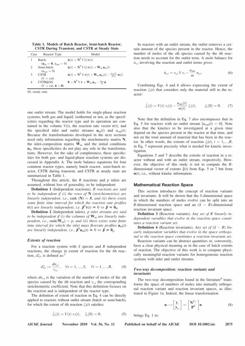
one outlet stream. The model holds for single-phase reactionsystems, both gas and liquid, isothermal or not, as the specif-icities regarding the reactor type and its operation are con-tained in the volume V(t), the reaction rate vector r(t), andthe specified inlet and outlet streams uin(t) and uout(t).Because the transformations developed in the next sectionsneed only information regarding the stoichometric matrix N,the inlet-composition matrix Win and the initial conditionsn0, these specificities do not play any role in the transforma-tions. However, for the sake of completeness, these specific-ities for both gas- and liquid-phase reaction systems are dis-cussed in Appendix A. The mole balance equations for fourcommon reactor types, namely batch reactor, semi-batch re-actor, CSTR during transient, and CSTR at steady state aresummarized in Table 1.

Throughout this article, the R reactions and p inlets areassumed, without loss of generality, to be independent:

Definition 1 (Independent reactions). R reactions are saidto be independent if (i) the rows of N (stoichiometries) arelinearly independent, i.e., rank (N) # R, and (ii) there existssome finite time interval for which the reaction rate profilesr(t) are linearly independent, i.e. bTr(t) 5 0 , b 5 0R.

Definition 2 (Independent inlets). p inlet streams are saidto be independent if (i) the columns of Win are linearly inde-pendent, i.e., rank(Win) # p, and (ii) there exists some finitetime interval for which the inlet mass flowrate profiles uin(t)are linearly independent, i.e., bTuin(t) 5 0 , b 5 0p.

Extents of reaction

For a reaction system with S species and R independentreactions, the change in extent of reaction for the ith reac-tion, dni, is defined as:2

dni :#dns;ims;i

; 8s # 1;…; S; 8i # 1;…;R; (4)

where dns,i is the variation of the number of moles of the sthspecies caused by the ith reaction and ms,i the correspondingstoichiometric coefficient. Note that this definition focuses onthe reaction and is independent of the reactor type.

The definition of extent of reaction in Eq. 4 can be directlyapplied to reactors without outlet stream (batch or semi-batch),for which the extent of ith reaction ni(t) satisfies:

_ni!t" # V!t" ri!t"; ni!0" # 0: (5)

In reactors with an outlet stream, the outlet removes a cer-tain amount of the species present in the reactor. Hence, thenumber of moles of the sth species caused by the ith reac-tion needs to account for the outlet term. A mole balance forns,i involving the reaction and outlet terms gives:

_ns;i # ms;i V ri %uoutm

ns;i: (6)

Combining Eqs. 4 and 6 allows expressing the extent ofreaction ni(t) that considers only the material still in the re-actor:

_ni!t" # V!t" ri!t" %uout!t"m!t"

ni!t"; ni!0" # 0: (7)

Note that the definition in Eq. 7 also encompasses that inEq. 5 for reactors with no outlet stream [uout(t) # 0]. Notealso that the kinetics to be investigated at a given timedepend on the species present in the reactor at that time, andnot on the total amount of material that has been in the reac-tor. In other words, the extents of reaction ni(t), i # 1,…,R,in Eq. 7 represent precisely what is needed for kinetic inves-tigation.

Equations 5 and 7 describe the extents of reaction in a re-actor without and with an outlet stream, respectively. How-ever, the objective of this study is not to compute the R-dimensional vector of extents n(t) from Eqs. 5 or 7 but fromn(t), i.e., without kinetic information.

Mathematical Reaction Space

This section introduces the concept of reaction variantsand invariants. It will be shown that the S-dimensional spacein which the numbers of moles evolve can be split into anR-dimensional reaction space and an (S % R)-dimensionalreaction invariant space.

Definition 3 (Reaction variants). Any set of R linearly in-dependent variables that evolve in the reaction space consti-tutes a reaction variant set.

Definition 4 (Reaction invariants). Any set of (S % R) lin-early independent variables that evolve in the space orthogo-nal to the reaction space constitutes a reaction invariant set.

Reaction variants can be abstract quantities or, conversely,have a clear physical meaning as in the case of batch extentsof reaction. The objective of this work is to compute physi-cally meaningful reaction variants for homogeneous reactionsystems with inlet and outlet streams.

Two-way decomposition: reaction variants andinvariants

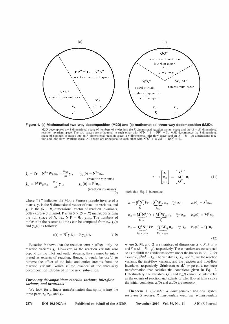
The two-way decomposition found in the literature6 trans-forms the space of numbers of moles into mutually orthogo-nal reaction variant and reaction invariant spaces, as illus-trated in Figure 1a. Indeed, the linear transformation

n%! yryiv

! "# NT$

PT

! "n (8)

brings Eq. 1 to:

Table 1. Models of Batch Reactor, Semi-batch Reactor,CSTR During Transient, and CSTR at Steady State

Case Reactor Type Model

1 Batch(uin # 0, uout # 0)

_n!t" # NT V!t" r!t"

2 Semi-batch(uout # 0)

_n!t" # NT V!t" r!t" $Win uin!t"

3 CSTR(V # cst)

_n!t" # NT V r!t" $Win uin!t" % uout!t"m!t" n!t"

4 CSTR@SS(V # cst, _n # 0)

0 # NT V r$Win uin % uoutm n

SS, steady state.

AIChE Journal November 2010 Vol. 56, No. 11 Published on behalf of the AIChE DOI 10.1002/aic 2875

_yr # Vr$ NT$Winuin %uoutm

yr; yr!0" # NT$n0;

!reaction variants"_yiv # PTWinuin %

uoutm

yiv; yiv!0" # PTn0;

!reaction invariants"!9"

where ‘‘$’’ indicates the Moore-Penrose pseudo-inverse of amatrix, yr is the R-dimensional vector of reaction variants, andyiv is the (S % R)-dimensional vector of reaction invariants,both expressed in kmol. P is an S & (S % R) matrix describingthe null space of N, i.e., N P # 0R&(S%R). The numbers ofmoles n in the reactor at time t can be computed from n0, yr(t)and yiv(t) as follows:

n!t" # NTyr!t" $ P yiv!t": (10)

Equation 9 shows that the reaction term r affects only thereaction variants yr. However, as the reaction variants alsodepend on the inlet and outlet streams, they cannot be inter-preted as extents of reaction. Hence, it would be useful toremove the effect of the inlet and outlet streams from thereaction variants, which is the essence of the three-waydecomposition introduced in the next subsection.

Three-way decomposition: reaction variants, inlet-flowvariants, and invariants

We look for a linear transformation that splits n into thethree parts zr, zin, and ziv,

n%!zrzinziv

2

4

3

5 #ST

MT

QT

2

4

3

5n; (11)

such that Eq. 1 becomes:

_zr # STNT|##{z##}

IR

Vr$ STWin|###{z###}0R&p

uin % uoutm zr; zr!0" # STn0;

_zin # MTNT|###{z###}0R&R

Vr$MTWin|###{z###}Ip

uin % uoutm zin; zin!0" # MTn0;

_ziv # QTNT

|##{z##}0!S%R%p"&R

Vr$ QTWin|###{z###}0!S%R%p"&p

uin % uoutm ziv; ziv!0" # QTn0;

(12)

where S, M, and Q are matrices of dimensions S & R, S & p,and S& (S% R% p), respectively. These matrices are constructedso as to fulfill the conditions shown under the braces in Eq. 12, forexample, STNT # IR. The variables zr, zin, and ziv are the reactionvariants, the inlet-flow variants, and the reaction and inlet-flowinvariants, respectively. Srinivasan et al.8 proposed a nonlineartransformation that satisfies the conditions given in Eq. 12.Unfortunately, the variables zr(t) and zin(t) cannot be interpretedas the extents of reaction and extents of inlet flow at time t sincethe initial conditions zr(0) and zin(0) are nonzero.

Theorem 1. Consider a homogeneous reaction systeminvolving S species, R independent reactions, p independent

Figure 1. (a) Mathematical two-way decomposition (M2D) and (b) mathematical three-way decomposition (M3D).M2D decomposes the S-dimensional space of numbers of moles into the R-dimensional reaction variant space and the (S % R)-dimensionalreaction invariant space. The two spaces are orthogonal to each other with NTNT$ 1 $ PPT # IS. M3D decomposes the S-dimensionalspace of numbers of moles into an R-dimensional reaction space, a p-dimensional inlet-flow space, and an (S % R % p)-dimensional reac-tion and inlet-flow invariant space. All spaces are orthogonal to each other with NTST $ WinM

T $ QQT # IS.

2876 DOI 10.1002/aic Published on behalf of the AIChE November 2010 Vol. 56, No. 11 AIChE Journal

inlets and one outlet, and let rank ([NT,Win]) # R $ p.Then, the linear transformation

n%!zrzinziv

2

4

3

5 #ST

MT

QT

2

4

3

5n (13)

brings Eq. 1 to:

_zr #Vr% uoutm zr; zr!0"# STn0; !reaction variants "

_zin # uin% uoutm zin; zin!0"#MTn0; !inlet-flow variants"

_ziv #%uoutm ziv; ziv!0"#QTn0:

!reaction andinlet-flow invariants"

(14)

zr is the R-dimensional vector of reaction variants expressedin kmol, zin the p-dimensional vector of inlet-flowvariants expressed in kg, and ziv the (S % R % p)-dimensionalvector of reaction and inlet-flow invariants expressed inkmol. The matrices S, M, and Q are computed using thealgorithm given in Appendix D. The numbers of moles n in thereactor at time t can be computed from zr(t), zin(t), and ziv(t) asfollows:

zrzinziv

2

4

3

5%! n!t" # NTzr!t" $Winzin!t" $Qziv!t": (15)

See Appendix B for proof.Interpretation. The three-way decomposition illustrated

in Figure 1b can be interpreted as follows. NTNT$,WinW

$in, and QQT represent the reaction, inlet-flow, and

reaction and inlet-flow invariant spaces, respectively. Byconstruction, QQT is orthogonal to both the reaction andinlet spaces, which leads to QTNT # 0(S%R%p) & R andQTWin # 0(S%R%p) & p in Eq. 12, and thus ziv is inde-pendent of r and uin. Furthermore, as the reaction andinlet spaces are not orthogonal to each other, the inletspace is rotated to give the rotated inlet space WinM

T

that fulfills the conditions MTNT # 0R and MTWin # Ipso that zin is independent of r and the inlet-flow variantsare decoupled. Finally, as the reaction space NTNT$ isnot orthogonal to WinM

T, the projection (IS % WinMT) is

introduced to make the reaction space NTST orthogonal tothe rotated inlet space, thus giving ST # NT$(IS %WinM

T) and STNT # IR. It follows that zr is independentof uin and the reaction variants are decoupled. Note thatthe vectors zin and ziv represent the (S % R) reactioninvariants that can be computed independently of thereaction rate expressions r. Note also that the effect ofthe outlet flow is still present in zr, zin, and ziv as seen inEq. 14. The linear transformation in Theorem 1 can bevisualized by rewriting Eq. 15 with the help of Eq. 13:

n # NTST $WinMT $QQT

$ %n # IS n: (16)

Computing Extents from the Numbersof Moles n(t)

The two-way and three-way decompositions presented inthe previous section have generated mathematical variantsand invariants that are devoid of a direct physical meaning.For example, due to the presence of nonzero initial condi-tions, the reaction and inlet-flow variants in Eq. 14 cannotbe interpreted as individual extents of reaction and inletflow. This section will propose a linear transformation ofthese reaction and flow variants to true extents of reactionand flow, thus paving the way to the computation of extentsfrom the numbers of moles n(t).

Discounting of initial conditions

For computing the extents of reaction and inlet flow, it isnecessary to account for the effect of the nonzero initial condi-tions in Eq. 14. At time 0, one needs to remove the contribu-tions zr,0 # STn0 and zin,0 # MTn0. However, the effect of theinitial conditions reduces with time due the presence of theoutlet stream. Hence, one needs to discount the effect of thenonzero initial conditions, which can be done with the intro-duction of the discounting variable k(t) [ [0,1] as shown next.The resulting linear transformation of zr, zin, and ziv reads:

zr

zin

ziv

2

64

3

75%!xr

xin

xiv

2

64

3

75 #zr

zin

ziv

2

64

3

75% k

zr;0

zin;0

ziv;0

2

64

3

75 with

k #1TS%R%pziv

1TS%R%pziv;0and 1TS%R%pziv;0 6# 0; !17"

where xr is the R-dimensional vector of extents of reaction, xinthe p-dimensional vector of extents of inlet flow, and xiv the (S %R % p)-dimensional vector of reaction and inlet-flow invariants.

From numbers of moles n(t) to extents x(t)

The linear transformation is described in the next theorem.The transformed reaction and inlet-flow invariant space isone-dimensional and can be described by the variable k. Itwill be shown that the condition 1TS–R–pziv,0 = 0 is satisfiedif and only if the initial numbers of moles n0 provide addi-tional information to the inlet-composition matrix Win or, inmathematical terms, Win and n0 are linearly independent ofeach other, i.e., rank([Win n0]) # p $ 1.

Theorem 2. Consider a homogeneous reaction systeminvolving S species, R independent reactions, p independentinlets and one outlet, and let rank([NT Win n0]) # R $ p $1. Then, the linear transformation

n%!xrxink

2

4

3

5 #ST0MT

0

qT0

2

4

3

5n; (18)

with

ST0 # ST!IS % n0 qT0 "; MT

0 # MT!IS % n0 qT0 ";

qT0 #1TS%R%pQ

T

1TS%R%pQTn0

; !19"

brings Eq. 1 to:

AIChE Journal November 2010 Vol. 56, No. 11 Published on behalf of the AIChE DOI 10.1002/aic 2877

_xr;i # V ri %uoutm

xr;i; xr;i!0" # 0; 8 i # 1;…;R;

!extents of reaction"_xin;j # uin;j %

uoutm

xin;j; xin;j!0" # 0; 8 j # 1;…; p;

!extents of inlet flow"_k # % uout

mk; k!0" # 1: !discounting of n0"

!20"

xr,i is the extent of reaction corresponding to the ith reactionexpressed in kmol, xin,j the extent of inlet flow correspondingto the jth inlet expressed in kg, and k the scalar dimensionlessvariable used to discount the effect of the initial conditions.The numbers of moles n in the reactor at time t can becomputed from xr(t), xin(t), and k(t) as follows:

xrxink

2

4

3

5%! n!t" # NTxr!t" $Winxin!t" $ n0k!t": (21)

See Appendix C for proof.Remarks. Several remarks are in order:1. It is convenient to express the transformed system

exclusively in terms of extents by introducing the dimension-less scalar extent of outlet flow xout(t) # 1 % k(t), withwhich Eq. 21 becomes:

xrxinxout

2

4

3

5%!n!t" # n0 $ NTxr!t" $Winxin!t" % n0xout!t":

(22)xout evolves also in the one-dimensional space n0qT0 .

2. The extent of reaction xr,i in Eq. 20 corresponds to niin Eq. 7.

3. Transformation (18) uses the knowledge of N, Win,and n0. Note that, compared to the transformation (11), thistransformation depends on the initial conditions n0, hencethe subscript 0 in the transformation matrices.

4. The transformed reaction system is of dimension R $p $ 1 and not S. The (S % R % p) invariant states xiv areidentically equal to zero and can be discarded:

xiv!t" # QT0n!t" # 0S%R%p; (23)

with QT0 # QT(IS % n0qT0 ).

5. The matrix (IS % n0qT0 ) removes the contribution of n0from zr, zin, and ziv to obtain xr, xin, and xiv. Hence, xrevolves in the R-dimensional space NTST0 , xin in the p-dimensional space WT

inMT0 , and xiv in the (S % R % p % 1)-

dimensional space QQT0 . k evolves in the one-dimensional

space n0qT0 . Note that the spaces for xr, xin, xiv, and k arenot orthogonal to each other, but they add up to the identitymatrix, i.e., NTST0 $ WinMT

0 $ QQT0 $ n0qT0 # IS.

6. It is well known22 that a nonzero n0 never lies in therow space of N. Thus, the working assumption of Theorem2, rank([NTWin n0]) # R $ p $ 1, implies rank([Win n0]) #p $ 1.

7. In the case where n0 is a linear combination of therows of Win, i.e., rank([Win n0]) # p, n0 can be modeled byan impulse inlet flowrate for the given Win. Hence, zr,0 # 0R

and zin,0 # 0p in the model (14), which generates the extentszr # xr and zin # xin.

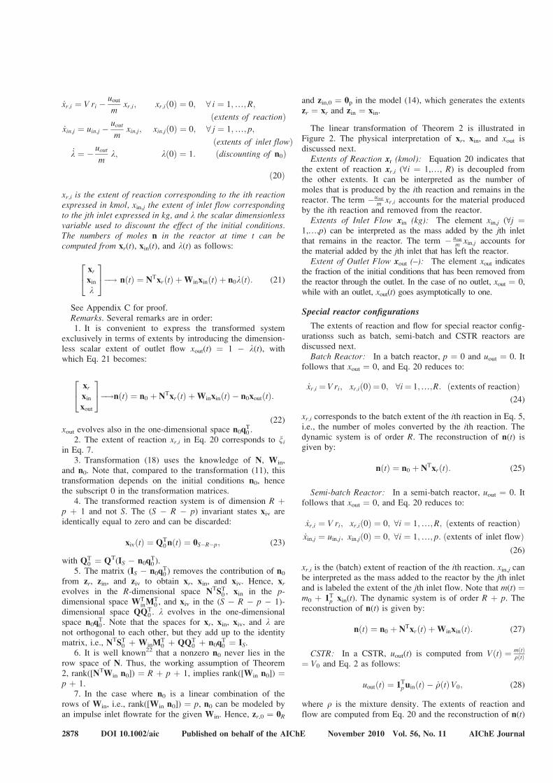
The linear transformation of Theorem 2 is illustrated inFigure 2. The physical interpretation of xr, xin, and xout isdiscussed next.

Extents of Reaction xr (kmol): Equation 20 indicates thatthe extent of reaction xr,i (Vi # 1,…, R) is decoupled fromthe other extents. It can be interpreted as the number ofmoles that is produced by the ith reaction and remains in thereactor. The term %uout

m xr;i accounts for the material producedby the ith reaction and removed from the reactor.

Extents of Inlet Flow xin (kg): The element xin,j (Vj #1,…,p) can be interpreted as the mass added by the jth inletthat remains in the reactor. The term % uout

m xin;j accounts forthe material added by the jth inlet that has left the reactor.

Extent of Outlet Flow xout (–): The element xout indicatesthe fraction of the initial conditions that has been removed fromthe reactor through the outlet. In the case of no outlet, xout # 0,while with an outlet, xout(t) goes asymptotically to one.

Special reactor configurations

The extents of reaction and flow for special reactor config-urationss such as batch, semi-batch and CSTR reactors arediscussed next.

Batch Reactor: In a batch reactor, p # 0 and uout # 0. Itfollows that xout # 0, and Eq. 20 reduces to:

_xr;i # V ri; xr;i!0" # 0; 8i# 1;…;R: !extents of reaction"(24)

xr,i corresponds to the batch extent of the ith reaction in Eq. 5,i.e., the number of moles converted by the ith reaction. Thedynamic system is of order R. The reconstruction of n(t) isgiven by:

n!t" # n0 $ NTxr!t": (25)

Semi-batch Reactor: In a semi-batch reactor, uout # 0. Itfollows that xout # 0, and Eq. 20 reduces to:

_xr;i # V ri; xr;i!0" # 0; 8i # 1;…;R; !extents of reaction"_xin;j # uin;j; xin;j!0" # 0; 8i # 1;…; p: !extents of inlet flow"

(26)

xr,i is the (batch) extent of reaction of the ith reaction. xin,j canbe interpreted as the mass added to the reactor by the jth inletand is labeled the extent of the jth inlet flow. Note that m(t) #m0 $ 1Tp xin(t). The dynamic system is of order R $ p. Thereconstruction of n(t) is given by:

n!t" # n0 $ NTxr!t" $Winxin!t": (27)

CSTR: In a CSTR, uout(t) is computed from V!t" # m!t"q!t"

# V0 and Eq. 2 as follows:

uout!t" # 1Tpuin!t" % _q!t"V0; (28)

where q is the mixture density. The extents of reaction andflow are computed from Eq. 20 and the reconstruction of n(t)

2878 DOI 10.1002/aic Published on behalf of the AIChE November 2010 Vol. 56, No. 11 AIChE Journal

is given by Eq. 22. The dynamic system is of order R $ p $ 1.Note that, if the density is constant, q(t) #q0, m(t) # m0 anduout(t) # 1Tp uin(t). It follows that k(t) can be computed

algebraically from the states xin(t) as k!t" # 1% 1Tp xin!t"m0

and,thus, the state equation for k can be removed and the dynamicsystem is of order R $ p.

Implications of Being Able to Compute x(t)from n(t)

The linear transformation proposed by Theorem 2 leads toextents of reaction and flow. Several implications are brieflydiscussed in the following sections.

Identification of reaction systems from measured data

The expressions V(t)ri(t), Vi # 1,…,R, and uin,j(t), Vj #1,…,p, can be computed from the measured numbers of molesn(t) and the knowledge of N, Win, and n0 using a differentialmethod.23 For batch reactors, for example, the product V(t) r(t)can be computed through differentiation of n(t) and knowledgeof N (see Table 1). However, the same task is more difficult insemi-batch and CSTR reactors because of the contributions ofthe inlet term Winuin(t) and outlet term uout!t"

m!t" n!t". If these termsare either known or measured, they can be accounted for andthe product Vr inferred from n(t). On the other hand, even ifthe inlet and outlet terms are unknown, the proposed lineartransformation (18) allows computing the individual extents of

reaction and flow from the measured n using an integralmethod. It is well-known that the integral method has statisticaladvantages over the differential method in the presence of onlya few noisy measurements of n.23 Then, in subsequent steps,reaction kinetics can be investigated individually for each reac-tion using for example the incremental identification approachproposed in Brendel et al.13

Model reduction

For batch and semi-batch reaction systems, a comparison ofEqs. 1 and 20 indicates that the number of state variables hasbeen reduced from S to (R $ p $ 1) for general open reactionsystems, and even further to R for batch and (R $ p) forsemi-batch and constant-density CSTR. The model order canalso be reduced by eliminating fast modes using, for example,singular perturbation theory.14,24 As the reactions (and not thenumbers of moles) exhibit the fast and slow dynamics behav-ior, the numbers of moles typically cannot be classified as fastor slow states and Eq. 1 is not suited for application of singu-lar perturbation theory. In contrast, the extents of reaction xrin Eq. 20 are direct functions of the reaction rates and, thus,can be separated into fast and slow dynamics.

Parametric sensitivity analysis

Parametric sensitivity is simplified by working with theextents of reaction instead of the numbers of moles since the

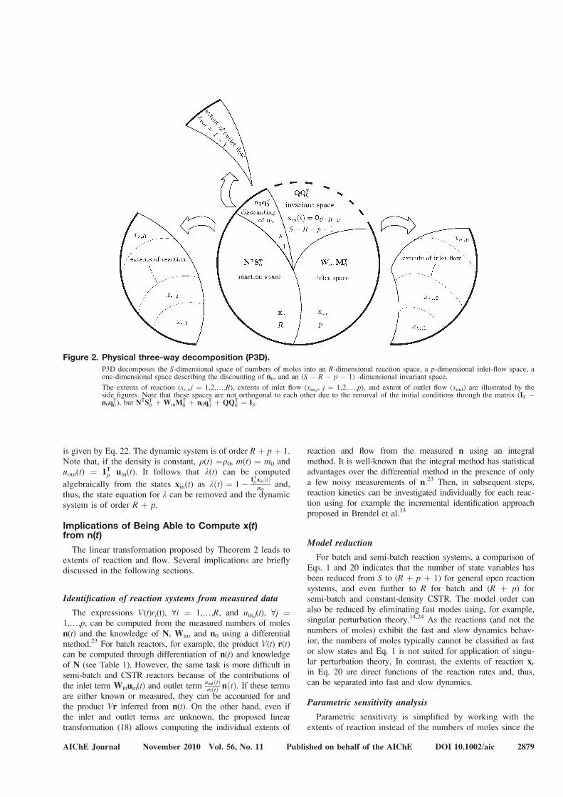
Figure 2. Physical three-way decomposition (P3D).P3D decomposes the S-dimensional space of numbers of moles into an R-dimensional reaction space, a p-dimensional inlet-flow space, aone-dimensional space describing the discounting of n0, and an (S % R % p % 1) -dimensional invariant space.

The extents of reaction (xr,i,i # 1,2,…,R), extents of inlet flow (xin,j, j # 1,2,…,p), and extent of outlet flow (xout) are illustrated by theside figures. Note that these spaces are not orthogonal to each other due to the removal of the initial conditions through the matrix (IS %n0qT0 ), but N

TST0 $ WinMT0 $ n0qT0 $ QQT

0 # IS.

AIChE Journal November 2010 Vol. 56, No. 11 Published on behalf of the AIChE DOI 10.1002/aic 2879

extent of reaction xr,i(t) contains all, but also only, informa-tion regarding V(t)ri(t). Another nice feature of the extentsof reaction is the fact that they are orthogonal to the inletspace, thereby leading to qxr/quin # 0R&p.

Parameter identification

The issue of parameter identification is related to paramet-ric sensitivity. As mentioned above, one can compute theindividual extents of reaction and inlet flow from the meas-ured data n(t). The resulting individual reaction rates V(t)ri(t), Vi # 1,…,R, can then be used to estimate the kineticparameters one reaction at a time and independently of theinlet and outlet flow patterns. Furthermore, it has been pro-posed to test possible model deficiencies by estimating ki-netic parameters.25 Since the stochastic error terms stemmainly from the parametric uncertainty of reaction rates, itis easier to associate stochastic terms to the individualextents of reaction xr,i, i # 1,…,R, than to n. This way, thesearch for possible model deficiencies can be limited to thetypically nonlinear expressions of reaction rates.

Illustrative Simulated Reaction Example

The implication of being able to compute the extents ofreaction and flow from measured data is illustrated through asimulated varying-density isothermal homogeneous reactionsystem. The reaction system considered is the ethanolysis ofphthalyl chloride (A).26 In two successive irreversible etha-nolysis reactions, the desired product phthalyl chloridemonoethyl ester (C) and phthalic diethylester (E) are pro-duced from ethanol (B). Both reactions produce hydrochloricacid (D). It is assumed that B also reacts with D in a reversi-ble side reaction to produce ethyl chloride (F) and water(G). The reaction system can be described by the followingreaction scheme with seven species (S # 7) and three inde-pendent reactions (R # 3):

R1: A$ B!r1 C$ D;

R2: C$ B!r2 E$ D;

R3: D$ B)r3F$ G:

The stoichiometric matrix isN#%1 %1 1 1 0 0 00 %1 %1 1 1 0 00 %1 0 %1 0 1 1

2

4

3

5

and the reaction rates obey the mass-action principle: r1 #j1 cAcB; r2 # j2 cBcC; r3 # j3 cBcD%j4 cFcG; with thereaction rate constants ji given in Table 2. The molecularweights and densities of the pure species are given in Table3. The vector of numbers of moles is n # [nA, nB, nC, nD,nE, nF, nG]

T. As the reactor is considered isothermal, the

density of the reaction mixture is computed asq# 1=

PSi#1

!wiqi, with !wi the weight fraction of species i.

Three reactor configurations will be investigated, namely abatch reactor, a semi-batch reactor, and the startup of aCSTR.

Case 1: Batch reactor

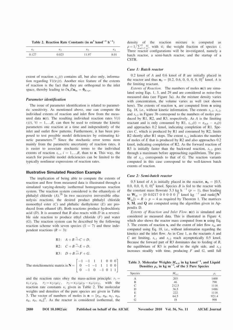
0.2 kmol of A and 0.6 kmol of B are initially placed inthe reactor and thus n0 # [0.2, 0.6, 0, 0, 0, 0, 0]T kmol. A isthe limiting reactant.

Extents of Reaction. The numbers of moles n(t) are simu-lated using Eqs. 1, 3, and 29 and are considered as noise-freemeasured data (see Figure 3a). As the mixture density varieswith concentration, the volume varies as well (not shownhere). The extents of reaction xr are computed from n usingEq. 18, i.e., without kinetic information. The extents xr,1, xr,2,and xr,3 in Figure 3b correspond to the numbers of moles pro-duced by R1, R2, and R3, respectively. As A is the limitingreactant and is only consumed by R1, xr,1(t) # nA,0 % nA(t)and approaches 0.2 kmol, indicating completion of R1. Spe-cies C, which is produced by R1 and consumed by R2, limitsR2 shortly after R1 stops. The extent xr,2 indicates the numberof moles of E that is produced by R2 and also approaches 0.2kmol, indicating completion of R2. As the forward reaction ofR3 is initially faster than the backward reaction, xr,3 goesthrough a maximum before approaching equilibrium. The pro-file of xr,3 corresponds to that of G. The reaction variantscomputed in this case correspond to the well-known batchextents of reaction.

Case 2: Semi-batch reactor

0.5 kmol of A is initially placed in the reactor, n0 # [0.5,0.0, 0,0, 0, 0, 0]T kmol. Species B is fed to the reactor withthe constant mass flowrate 5.3 kg h %1 (p # 1), thus leadingto Win # [0 0.0217 0 0 0 0 0 ]T kmol kg %1 and rank([NT

Win]) # R $ p # 4 as required by Theorem 1. The matricesS, M, and Q are computed using the algorithm given in Ap-pendix D.

Extents of Reaction and Inlet Flow. n(t) is simulated andconsidered as measured data. This is illustrated in Figure 4,which also shows the reactor mass computed from n using Eq.3. The extents of reaction xr and the extent of inlet flow xin arecomputed using Eq. 18, i.e., without information regarding thekinetics and the inlet flow. As in Case 1, as the reactants A andC are limiting, xr,1 and xr,2 reach asymptotically 0.5 kmol.Because the forward part of R3 dominates due to feeding of B,the equilibrium of R3 is pushed to the right side, and xr,3increases steadily with time, producing F and G, until full

Table 2. Reaction Rate Constants (in m3 kmol21 h21)

j1 j2 j3 j4

0.127 0.023 11.97 8.01

Table 3. Molecular Weights Mw,i, in kg kmol21, and LiquidDensities qi, in kg m23, of the S Pure Species

Species Mw,i qi

A 203 1400B 46 790C 212.5 1118D 36.5 1486E 222 1118F 64.5 921.4G 18 998

2880 DOI 10.1002/aic Published on behalf of the AIChE November 2010 Vol. 56, No. 11 AIChE Journal

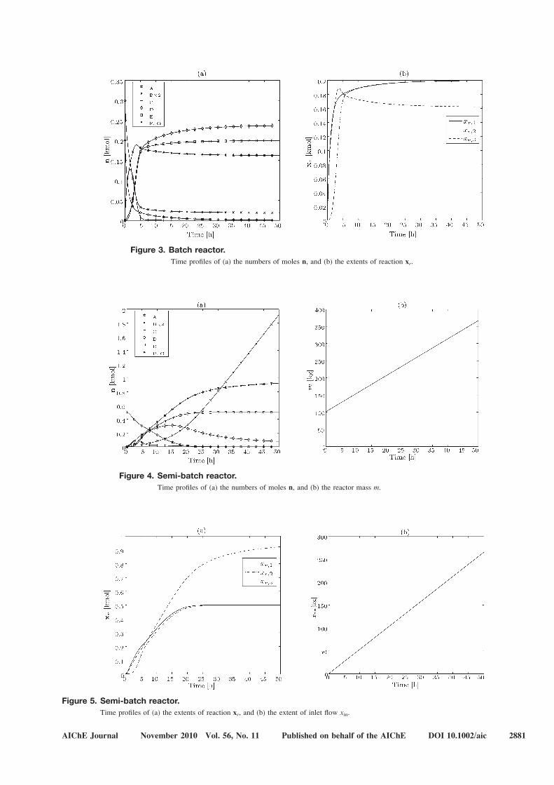
Figure 4. Semi-batch reactor.Time profiles of (a) the numbers of moles n, and (b) the reactor mass m.

Figure 5. Semi-batch reactor.Time profiles of (a) the extents of reaction xr, and (b) the extent of inlet flow xin.

Figure 3. Batch reactor.Time profiles of (a) the numbers of moles n, and (b) the extents of reaction xr.

AIChE Journal November 2010 Vol. 56, No. 11 Published on behalf of the AIChE DOI 10.1002/aic 2881

depletion of D (not shown here). As shown in Figure 5b, xinincreases steadily with time due to feeding of B.

Case 3: Startup of CSTR

There are two inlets to the CSTR (p # 2): pure phthalyldichloride A and pure ethanol B, thus leading to Win #

0:0049 0 0 0 0 0 00 0:0217 0 0 0 0 0

#T2

4 kmol kg%1 and

rank([NT Win]) # R $ p # 5.

The reactor is initially filled with 1.5 kmol of ethyl chlo-ride (F) and thus n0 # [0, 0, 0, 0, 0, 1.5, 0]T kmol. SpeciesA is fed with the constant mass flowrate 7.8 kg h%1, whilefeeding of B with the constant mass flowrate 5.3 kg h%1

starts after 5 h (p # 2). Hence, there is no reaction in theinterval [0, 5] h. The time profiles of n simulated using Eq.1 are shown in Figure 6a, the mass m computed using Eq. 3is shown in Figure 6b, and the inlet and outlet streams areshown in Figure 6c. Note that the outlet flowrate varies evenwhen the inlet flows are constant. Indeed, feeding the heavyspecies A increases the density of the reaction mixturewhich, according to Eq. 28, decreases the outlet mass flow-

rate. Addition of the light species B to the reactor after t #5 h initially decreases the density and thus also the reactormass. Thereafter, the reactions produce heavy species, whichincreases m.

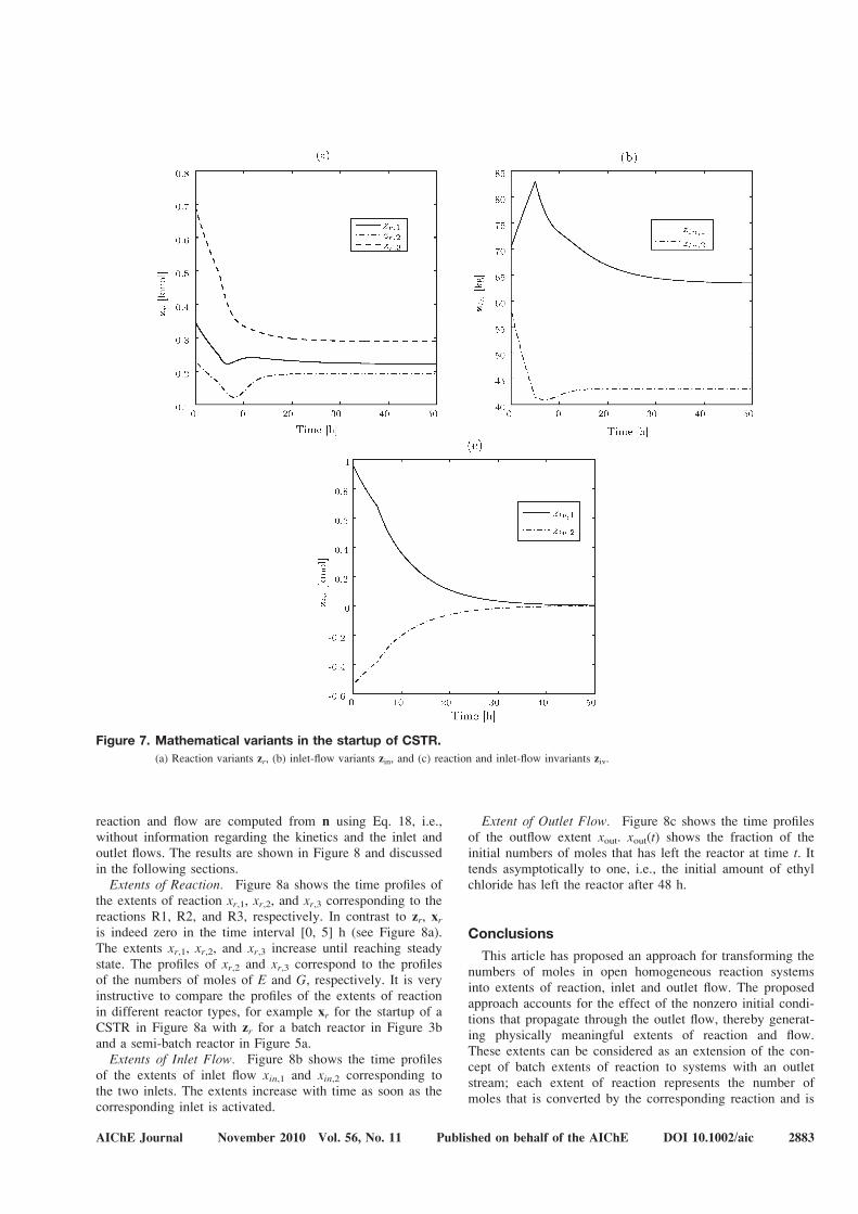
Mathematical Reaction Space. The transformation matri-ces S, M, and Q are calculated using the algorithm given inAppendix D. Transformation (13) is first applied to n to com-pute the reaction variants zr, the inlet-flow variants zin, and thereaction and flow invariants ziv (see Figure 7a–c). Figure 7ashows that all reaction variants take nonzero (positive) valuesin the time interval [0, 5] h despite the absence of reaction.This behavior results from the effect of the nonzero initial con-dition STn0. Similarly, zin,2 (corresponding to the feed of B)takes nonzero values in the same time interval despite the ab-sence of feed B. This behavior is due to the effect of the non-zero initial conditions MTn0. Hence, unlike in batch and semi-batch reactors, the mathematical reaction variants zr and theinlet-flow variants zin do not represent physical extents in reac-tion systems with an outlet stream.

Extents of reaction and flow The matrix Q and M arecalculated using the algorithm given in Appendix D. Asrank([NT Win n0]) # R $ p $ 1 # 6 and 1TS%R%pQ

Tn0 #0.4160 = 0, Theorem 2 can be applied. The extents of

Figure 6. Startup of CSTR.Time profiles of (a) the numbers of moles n, (b) the reactor mass m, and (c) the inlet and outlet mass flowrates uin,1, uin,2, and uout.

2882 DOI 10.1002/aic Published on behalf of the AIChE November 2010 Vol. 56, No. 11 AIChE Journal

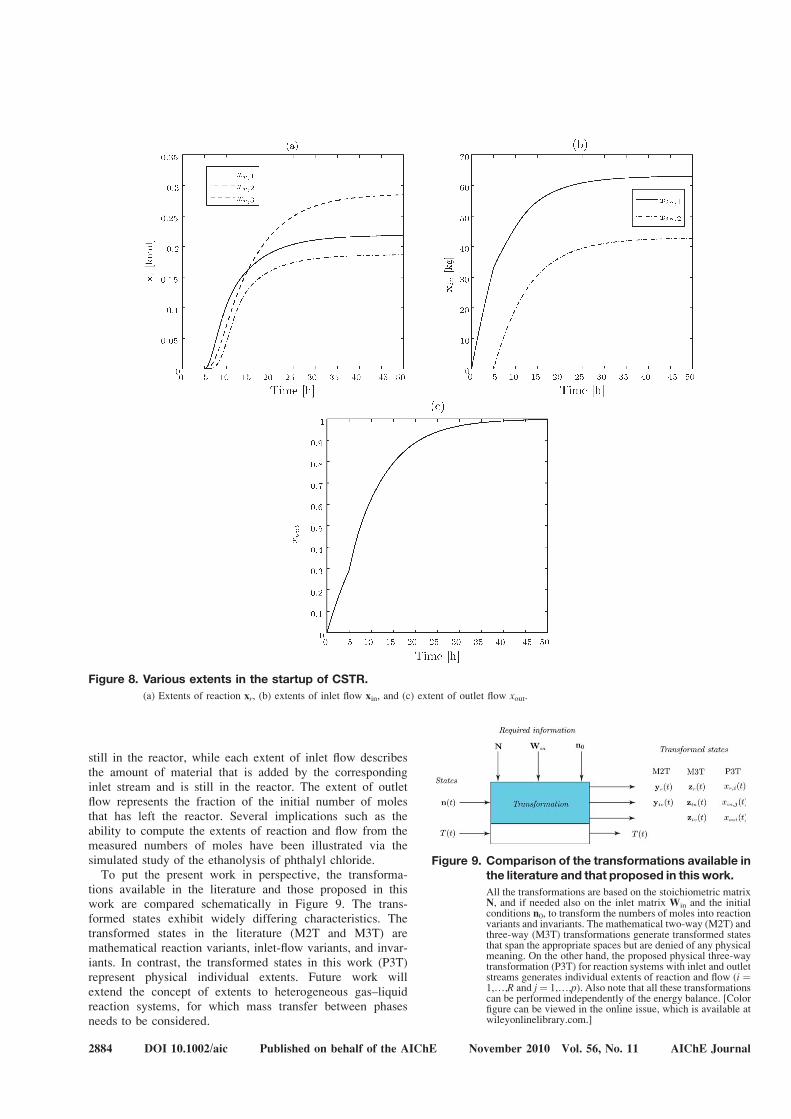
reaction and flow are computed from n using Eq. 18, i.e.,without information regarding the kinetics and the inlet andoutlet flows. The results are shown in Figure 8 and discussedin the following sections.

Extents of Reaction. Figure 8a shows the time profiles ofthe extents of reaction xr,1, xr,2, and xr,3 corresponding to thereactions R1, R2, and R3, respectively. In contrast to zr, xris indeed zero in the time interval [0, 5] h (see Figure 8a).The extents xr,1, xr,2, and xr,3 increase until reaching steadystate. The profiles of xr,2 and xr,3 correspond to the profilesof the numbers of moles of E and G, respectively. It is veryinstructive to compare the profiles of the extents of reactionin different reactor types, for example xr for the startup of aCSTR in Figure 8a with zr for a batch reactor in Figure 3band a semi-batch reactor in Figure 5a.

Extents of Inlet Flow. Figure 8b shows the time profilesof the extents of inlet flow xin,1 and xin,2 corresponding tothe two inlets. The extents increase with time as soon as thecorresponding inlet is activated.

Extent of Outlet Flow. Figure 8c shows the time profilesof the outflow extent xout. xout(t) shows the fraction of theinitial numbers of moles that has left the reactor at time t. Ittends asymptotically to one, i.e., the initial amount of ethylchloride has left the reactor after 48 h.

Conclusions

This article has proposed an approach for transforming thenumbers of moles in open homogeneous reaction systemsinto extents of reaction, inlet and outlet flow. The proposedapproach accounts for the effect of the nonzero initial condi-tions that propagate through the outlet flow, thereby generat-ing physically meaningful extents of reaction and flow.These extents can be considered as an extension of the con-cept of batch extents of reaction to systems with an outletstream; each extent of reaction represents the number ofmoles that is converted by the corresponding reaction and is

Figure 7. Mathematical variants in the startup of CSTR.(a) Reaction variants zr, (b) inlet-flow variants zin, and (c) reaction and inlet-flow invariants ziv.

AIChE Journal November 2010 Vol. 56, No. 11 Published on behalf of the AIChE DOI 10.1002/aic 2883

still in the reactor, while each extent of inlet flow describesthe amount of material that is added by the correspondinginlet stream and is still in the reactor. The extent of outletflow represents the fraction of the initial number of molesthat has left the reactor. Several implications such as theability to compute the extents of reaction and flow from themeasured numbers of moles have been illustrated via thesimulated study of the ethanolysis of phthalyl chloride.

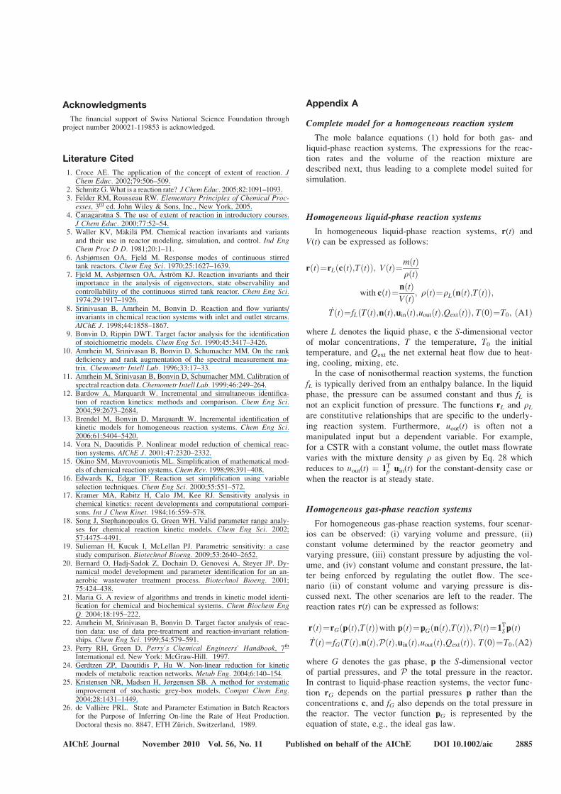
To put the present work in perspective, the transforma-tions available in the literature and those proposed in thiswork are compared schematically in Figure 9. The trans-formed states exhibit widely differing characteristics. Thetransformed states in the literature (M2T and M3T) aremathematical reaction variants, inlet-flow variants, and invar-iants. In contrast, the transformed states in this work (P3T)represent physical individual extents. Future work willextend the concept of extents to heterogeneous gas–liquidreaction systems, for which mass transfer between phasesneeds to be considered.

Figure 8. Various extents in the startup of CSTR.(a) Extents of reaction xr, (b) extents of inlet flow xin, and (c) extent of outlet flow xout.

Figure 9. Comparison of the transformations available inthe literature and that proposed in this work.All the transformations are based on the stoichiometric matrixN, and if needed also on the inlet matrix Win and the initialconditions n0, to transform the numbers of moles into reactionvariants and invariants. The mathematical two-way (M2T) andthree-way (M3T) transformations generate transformed statesthat span the appropriate spaces but are denied of any physicalmeaning. On the other hand, the proposed physical three-waytransformation (P3T) for reaction systems with inlet and outletstreams generates individual extents of reaction and flow (i #1,…,R and j# 1,…,p). Also note that all these transformationscan be performed independently of the energy balance. [Colorfigure can be viewed in the online issue, which is available atwileyonlinelibrary.com.]

2884 DOI 10.1002/aic Published on behalf of the AIChE November 2010 Vol. 56, No. 11 AIChE Journal

Acknowledgments

The financial support of Swiss National Science Foundation throughproject number 200021-119853 is acknowledged.

Literature Cited

1. Croce AE. The application of the concept of extent of reaction. JChem Educ. 2002;79:506–509.

2. Schmitz G.What is a reaction rate? J Chem Educ. 2005;82:1091–1093.3. Felder RM, Rousseau RW. Elementary Principles of Chemical Proc-

esses, 3rd ed. John Wiley & Sons, Inc., New York, 2005.4. Canagaratna S. The use of extent of reaction in introductory courses.

J Chem Educ. 2000;77:52–54.5. Waller KV, Makila PM. Chemical reaction invariants and variants

and their use in reactor modeling, simulation, and control. Ind EngChem Proc D D. 1981;20:1–11.

6. Asbjørnsen OA, Fjeld M. Response modes of continuous stirredtank reactors. Chem Eng Sci. 1970;25:1627–1639.

7. Fjeld M, Asbjørnsen OA, Astrom KJ. Reaction invariants and theirimportance in the analysis of eigenvectors, state observability andcontrollability of the continuous stirred tank reactor. Chem Eng Sci.1974;29:1917–1926.

8. Srinivasan B, Amrhein M, Bonvin D. Reaction and flow variants/invariants in chemical reaction systems with inlet and outlet streams.AIChE J. 1998;44:1858–1867.

9. Bonvin D, Rippin DWT. Target factor analysis for the identificationof stoichiometric models. Chem Eng Sci. 1990;45:3417–3426.

10. Amrhein M, Srinivasan B, Bonvin D, Schumacher MM. On the rankdeficiency and rank augmentation of the spectral measurement ma-trix. Chemometr Intell Lab. 1996;33:17–33.

11. Amrhein M, Srinivasan B, Bonvin D, Schumacher MM. Calibration ofspectral reaction data. Chemometr Intell Lab. 1999;46:249–264.

12. Bardow A, Marquardt W. Incremental and simultaneous identifica-tion of reaction kinetics: methods and comparison. Chem Eng Sci.2004;59:2673–2684.

13. Brendel M, Bonvin D, Marquardt W. Incremental identification ofkinetic models for homogeneous reaction systems. Chem Eng Sci.2006;61:5404–5420.

14. Vora N, Daoutidis P. Nonlinear model reduction of chemical reac-tion systems. AIChE J. 2001;47:2320–2332.

15. Okino SM, Mavrovouniotis ML. Simplification of mathematical mod-els of chemical reaction systems.Chem Rev. 1998;98:391–408.

16. Edwards K, Edgar TF. Reaction set simplification using variableselection techniques. Chem Eng Sci. 2000;55:551–572.

17. Kramer MA, Rabitz H, Calo JM, Kee RJ. Sensitivity analysis inchemical kinetics: recent developments and computational compari-sons. Int J Chem Kinet. 1984;16:559–578.

18. Song J, Stephanopoulos G, Green WH. Valid parameter range analy-ses for chemical reaction kinetic models. Chem Eng Sci. 2002;57:4475–4491.

19. Sulieman H, Kucuk I, McLellan PJ. Parametric sensitivity: a casestudy comparison. Biotechnol Bioeng. 2009;53:2640–2652.

20. Bernard O, Hadj-Sadok Z, Dochain D, Genovesi A, Steyer JP. Dy-namical model development and parameter identification for an an-aerobic wastewater treatment process. Biotechnol Bioeng. 2001;75:424–438.

21. Maria G. A review of algorithms and trends in kinetic model identi-fication for chemical and biochemical systems. Chem Biochem EngQ. 2004;18:195–222.

22. Amrhein M, Srinivasan B, Bonvin D. Target factor analysis of reac-tion data: use of data pre-treatment and reaction-invariant relation-ships. Chem Eng Sci. 1999;54:579–591.

23. Perry RH, Green D. Perry’s Chemical Engineers’ Handbook, 7th

International ed. New York: McGraw-Hill. 1997.24. Gerdtzen ZP, Daoutidis P, Hu W. Non-linear reduction for kinetic

models of metabolic reaction networks. Metab Eng. 2004;6:140–154.25. Kristensen NR, Madsen H, Jørgensen SB. A method for systematic

improvement of stochastic grey-box models. Comput Chem Eng.2004;28:1431–1449.

26. de Valliere PRL. State and Parameter Estimation in Batch Reactorsfor the Purpose of Inferring On-line the Rate of Heat Production.Doctoral thesis no. 8847, ETH Zurich, Switzerland, 1989.

Appendix A

Complete model for a homogeneous reaction system

The mole balance equations (1) hold for both gas- andliquid-phase reaction systems. The expressions for the reac-tion rates and the volume of the reaction mixture aredescribed next, thus leading to a complete model suited forsimulation.

Homogeneous liquid-phase reaction systems

In homogeneous liquid-phase reaction systems, r(t) andV(t) can be expressed as follows:

r!t"#rL!c!t";T!t""; V!t"#m!t"q!t"

with c!t"#n!t"V!t"

; q!t"#qL!n!t";T!t"";

_T!t"#fL!T!t";n!t";uin!t";uout!t";Qext!t""; T!0"#T0; !A1"

where L denotes the liquid phase, c the S-dimensional vectorof molar concentrations, T the temperature, T0 the initialtemperature, and Qext the net external heat flow due to heat-ing, cooling, mixing, etc.In the case of nonisothermal reaction systems, the function

fL is typically derived from an enthalpy balance. In the liquidphase, the pressure can be assumed constant and thus fL isnot an explicit function of pressure. The functions rL and qLare constitutive relationships that are specific to the underly-ing reaction system. Furthermore, uout(t) is often not amanipulated input but a dependent variable. For example,for a CSTR with a constant volume, the outlet mass flowratevaries with the mixture density q as given by Eq. 28 whichreduces to uout(t) # 1Tp uin(t) for the constant-density case orwhen the reactor is at steady state.

Homogeneous gas-phase reaction systems

For homogeneous gas-phase reaction systems, four scenar-ios can be observed: (i) varying volume and pressure, (ii)constant volume determined by the reactor geometry andvarying pressure, (iii) constant pressure by adjusting the vol-ume, and (iv) constant volume and constant pressure, the lat-ter being enforced by regulating the outlet flow. The sce-nario (ii) of constant volume and varying pressure is dis-cussed next. The other scenarios are left to the reader. Thereaction rates r(t) can be expressed as follows:

r!t"#rG!p!t";T!t""with p!t"#pG!n!t";T!t"";P!t"#1TSp!t"_T!t"#fG!T!t";n!t";P!t";uin!t";uout!t";Qext!t""; T!0"#T0;!A2"

where G denotes the gas phase, p the S-dimensional vectorof partial pressures, and P the total pressure in the reactor.In contrast to liquid-phase reaction systems, the vector func-tion rG depends on the partial pressures p rather than theconcentrations c, and fG also depends on the total pressure inthe reactor. The vector function pG is represented by theequation of state, e.g., the ideal gas law.

AIChE Journal November 2010 Vol. 56, No. 11 Published on behalf of the AIChE DOI 10.1002/aic 2885

Appendix B

Proof of Theorem 1

Let the S & (S % R % p) matrix Q, the S & p matrix Land the S & p matrix M obey the following conditions:C1: The S & S matrix [NT L Q] is of rank S,C2: The columns of Q are orthonormal and span the null

space of [NT Win]T,

C3: The columns of L are orthonormal and span the nullspace of [NT Q]T,C4: MTWin # Ip, which can be achieved by choosing M

# L(WTinL)

$.With ST # NT$(IS % WinM

T), the conditions C1–C4enforce the conditions shown under the braces in Eq. 12.Applying the transformation (13) to Eq. 1 gives:

_zr # Vr% uoutm

zr; zr!0" # STn0;

_zin # uin %uoutm

zin; zin!0" # MTn0;

_ziv # % uoutm

ziv; ziv!0" # QTn0:

(B1)

Next, Eq. 15 needs to be proven. For this, the followingproperties resulting from Conditions C1–C4 are used:

NTN$T$LLT$QQT#IS!complementaryorthonormal spaces";QQTWinM

T#0S&S !inlet space rotatedorthogonally toQQT byconstructionofM#L!WT

inL"$";

LLTWinMT#LLT !equivalent spaces":

(B2)Premultiplying both sides of Eq. 13 with [NT Win Q]

gives:

NTzr $Winzin $Qziv # !NTST $WinMT $QQT" n

# !NTNT$ !IS %WinMT" $WinM

T $QQT"n# !NTNT$ $ !LLT $QQT"WinM

T $QQT" n# !NTNT$ $ LLT $QQT"n # n

()n # NTzr $Win zin $Qziv: !B3"

An algorithm for computing the matrices S, M, and Q isgiven in Appendix D.

Appendix C

Proof of Theorem 2

The proof has three parts. In the first part of the proof, itis shown that 1T!S%R%p" QTn0 = 0 is guaranteed through theworking assumption rank([NT Win n0]) # R $ p $ 1. Thisassumption indicates that n0 does not belong to the columnspace of [NT Win], which, with Condition C2, is equivalentto saying that n0 does not belong to the null space of QT.Hence, QT n0 = 0S%R%p. As Q is of full rank (S % R % p),1T!S%R%p" Q

T = 0S and 1T!S%R%p" QT n0 = 0 follow.

In the second part of the proof, Eqs. 20 and 23 arederived. For this, the following properties resulting fromConditions C1–C4 are used: qT0N

T # 0TR, qT0Win # 0Tp , and

qT0 n0 # 1. Applying the transformation (18) and

xiv # QT0n with QT

0 # QT!IS % n0 qT0 " (C1)

to Eq. 1 gives:

_xr # V r% uoutm

xr; xr!0" # 0R;

_xin # uin %uoutm

xin; xin!0" # 0p;

_k # % uoutm

k; k!0" # 1;

_xiv # % uoutm

xiv; xiv!0" # 0S%R%p:

(C2)

As xiv(0) # 0S%R%p, xiv(t) # 0S%R%p for all time t. Hence,xiv can be dropped from Eq. C2.In the last part of the proof, Eq. 21 is derived. For this,

the following properties are used: (i) Eq. B2, (ii) Qxiv(t) #0S as xiv(t) # 0S%R%p, and (iii) (NTST $ WinM

T $ QQT) #IS from Eq. B3. Premultiplying both sides of Eq. 18 with[NT Win n0] leads to:

NTxr $Winxin $ kn0 # NTxr $Winxin $ kn0 $Qxiv

# !NTST $WinMT $QQT"!IS % n0 q

T0 " n$ n0q

T0n

# !IS % n0 qT0 " n$ n0q

T0n # n

()n!t" # NTxr!t" $Winxin!t" $ n0 k!t":(C3)

Appendix D

Algorithm to compute S, M, and Q

The algorithm assumes rank([NT Win]) # R $ p, althoughit can easily be extended to the case of rank([NT Win]) \ R$ p. The objective is to compute the matrices Q, L, M, andS that fulfill the conditions C1–C4 given in Appendix B.

1. Apply the singular value decomposition (SVD) to thematrix [NT Win]:

'NT Win( # U1S1VT1 :

Let U1 # [U1,1 U1,2], where U1,1 and U1,2 are of dimen-sion S & (R $ p) and S & (S % R % p), respectively. Then,Q # U1,2.

2. Note that rank([NT Q]) # S % p. Apply SVD to thematrix [NTQ]:

'NT Q( # U2S2VT2 :

Let U2 # [U2,1 U2,2], where U2,1 and U2,2 are of dimen-sion S & (S % p) and S & p, respectively. Then, L #U2,2.

3. Compute M # L(WTinL)

$.4. Compute ST # NT$(IS % WinM

T).

Manuscript received May 29, 2009, revision received Aug. 20, 2009, and finalrevision received Jan. 18, 2010.

2886 DOI 10.1002/aic Published on behalf of the AIChE November 2010 Vol. 56, No. 11 AIChE Journal