Theoretical Economics 1 (2006), 143–166 1555-7561/20060143

Competitive markets with externalities

MITSUNORI NOGUCHI

Department of Economics, Meijo University

WILLIAM R. ZAME

Department of Economics, University of California, Los Angeles

This paper presents a general model of a competitive market with consumptionexternalities, and establishes the existence of equilibrium in the model, under as-sumptions comparable to those in classical models. The model allows productionand indivisible goods. Examples illustrate the generality and applicability of theresults.

KEYWORDS. Competitive equilibrium, externalities, distributional economies.

JEL CLASSIFICATION. D5.

1. INTRODUCTION

The classical model of competitive markets assumes that agents care only about theirown consumption. However, the consumption of others may matter to me, because Iam altruistic or spiteful, because I am a slave to fashion or a radical non-conformist—or because the consumption of others impinges on my own: my neighbors’ use of coalto heat their houses pollutes the air I breathe; their use of household security servicesmakes mine safer. For environments with a finite number of agents, it has been knownfor a long time that consumption externalities can be accommodated in a consistentmarket model. (See Shafer and Sonnenschein 1975 for the first proof and Laffont 1977for discussion and applications.) However such models are not entirely satisfactory be-cause they require individual preferences to be convex and exclude indivisible goods.(As Starrett 1972 argues, requiring individual preferences to be convex is especially prob-lematical in the presence of consumption externalities.) Moreover, the price-taking as-sumptions inherent in the notion of competitive equilibrium are incompatible with the

Mitsunori Noguchi: noguchi@ccmfs.meijo-u.ac.jpWilliam R. Zame: zame@econ.ucla.eduEarlier versions circulated under the title “Equilibrium Distributions with Externalities.” We thank RobertAnderson for several enlightening conversations, and the Co-Editor Ed Green and several anonymous ref-erees for very useful suggestions. Zame gratefully acknowledges financial support from the John SimonGuggenheim Foundation, the National Science Foundation (under grants SES-0079299 and SES-0317752),the UCLA Academic Senate Committee on Research, and the Caltech Social and Information Sciences Lab-oratory, and Caltech for sabbatical hospitality. Views expressed here are those of the authors and do notnecessary reflect the views of any funding agency.

Copyright c© 2006 Mitsunori Noguchi and William R. Zame. Licensed under the Creative CommonsAttribution-NonCommercial License 2.5. Available at http://econtheory.org.

144 Noguchi and Zame Theoretical Economics 1 (2006)

presence of agents who have market power—as all agents typically do when the totalnumber of agents is finite.

Absent externalities, the work of Aumann (1964, 1966) and subsequent authors hasshown that non-convex preferences, indivisible goods, and infinitesimal agents whohave no market power are easily accommodated in a model with a continuum of agents.However, a satisfactory model that also incorporates consumption externalities hasproved surprisingly elusive. This paper provides such a model.

The key to our approach is that we abandon Aumann’s descriptions of the econ-omy and of equilibrium in terms of maps from agent names to agent characteristicsand consumptions, and instead use the descriptions (introduced by Hart et al. 1974) ofthe economy and of equilibrium in terms of probability distributions on agent charac-teristics and on agent characteristics and choices. In other words, our description isdistributional rather than individualistic. This choice is born of necessity: as we showby examples, if we were to insist on an individualistic description of equilibrium thenwe would quickly be confronted with simple economies that admit no equilibrium atall. By contrast, our distributional approach, although perhaps less familiar than theindividualistic approach, leads to a clean and elegant framework, easily accommodatesboth production and indivisible goods, and satisfies the basic consistency requirementthat equilibrium exist.

A simple example, elaborated in Section 2, may help to orient the reader. Consider alarge number of individuals who live on the bank of a long river. Each individual tradesand consumes goods, but the waste products of that consumption create harmful pol-lution for everyone downstream. As we show, if we wish to guarantee that such an econ-omy admits an equilibrium we must accept the possibility that two individuals who livein the same location, have the same preferences, are entitled to the same endowment,and experience the same externality, still choose different consumption bundles.

Previous papers on continuum economies with externalities all take Aumann’s in-dividualistic approach, and treat only exchange economies with divisible goods. Ham-mond et al. (1989) show that equilibrium allocations coincide with the f-core (a variationof the usual core in which improving coalitions are required to be finite). However, as ourexamples show, in their model, equilibrium may not exist and the f-core may be empty.Noguchi (2005) and Cornet and Topuzu (2005) prove that equilibrium exists if individ-ual preferences are convex in own consumption and weakly continuous in others’ con-sumptions. As we have noted, requiring that individual preferences be convex vitiatesan important reason for treating continuum economies, and certainly excludes indivis-ibilities. As we discuss later, in the individualistic framework the requirement of weakcontinuity restricts the externalities agents experience to be linear in the consumptionof others. Our examples in Section 5 show that, absent any of these assumptions, indi-vidualistic equilibrium need not exist. Balder (2003) demonstrates that equilibrium ex-ists if the externality enters into the preferences of each individual in the same way. Thisrequirement would seem to exclude all local externalities, all externalities that diminishwith distance, and all externalities that have any directional aspect—indeed, most ex-ternalities that arise in practice. By contrast, our results allow for indivisible goods, for

Theoretical Economics 1 (2006) Competitive markets with externalities 145

individual preferences that are not convex, and for general externalities that each agentexperiences in a unique way.

Following this Introduction, we begin with an informal elaboration of the orientingexample mentioned above. The detailed description of the model is in Section 3 and theexistence theorem is in Section 4. Section 5 presents a number of illustrative examples.Proofs are collected in Appendix A. Appendix B sketches an alternative model, in whichthe consumption of others enters individual preferences as a parameter.

2. AN ORIENTING EXAMPLE

To orient the reader, we begin by describing, in the familiar individualistic framework,a simple economy that has no individualistic equilibrium. Our description is a bitinformal.

EXAMPLE 1. We consider a large number of agents living on the banks of a long river. Weidentify locations with the interval T = [0, 1], and assume the population is uniformlydistributed along the river, so the population measure τ is Lebesgue measure.

There are two commodities, each perfectly divisible. Each agent is endowed withone unit of each good: e (t ) ≡ (1, 1). Agents derive utility from their own consumption,but suffer a pollution externality from the consumption of others who live upstreamfrom them. If we choose directions so that upstream from s means to the left of s , andwrite f (t ) = ( f 1(t ), f 2(t )) for the consumption of an agent located at t , then the external-ity experienced by an agent located at s is

η(s , f ) =

∫ s

0

f (t )dt .

Note that η is two-dimensional; write η = (η1,η2) for the components of η. The utilityof an agent located at s who consumes the bundle (x1,x2) when the consumption of allagents is described by f is

u s (x1,x2, f ) = [2−η1(s , f )]x 21 +[2−η2(s , f )]x 2

2 .

Note that η1(s , f ) ≤ 1 for each i and that the exponents of x1,x2 are greater than 1, soutility is strictly increasing and convex in own consumption. In particular, individualpreferences are not convex.

In the individualistic framework, an equilibrium consists of prices p1, p2 (withoutloss, normalize so that p1+p2 = 1) and a consumption allocation f = ( f 1, f 2) : T → R2

+so that almost every agent optimizes in his/her budget set and the market clears. Weclaim that no such equilibrium exists.

To see this, note first that each agent’s wealth is p1 · 1+p2 · 1 = 1. Because the totalsupply of each good is 1, ηi ≤ 1 for each i , so utility functions display increasing returnsto scale in consumption of each good, and the optimal choice for an agent located at s isalways either (1/p1, 0) or (0, 1/p2). (Of course the agent may be indifferent between the

146 Noguchi and Zame Theoretical Economics 1 (2006)

two choices.) An agent located at s strictly prefers (1/p1, 0) if and only if

2−η1(s , f )p1

>2−η2(s , f )

p2.

Similarly, an agent located at s strictly prefers (0, 1/p2) if and only if

2−η1(s , f )p1

<2−η2(s , f )

p2.

Set

G1 =�

s ∈ [0, 1] :2−η1(s , f )

p1>

2−η2(s , f )p2

�

G2 =�

s ∈ [0, 1] :2−η1(s , f )

p1<

2−η2(s , f )p2

�

I =�

s ∈ [0, 1] :2−η1(s , f )

p1=

2−η2(s , f )p2

�

.

These sets are disjoint and their union is [0, 1]. Because Lebesgue measure τ is non-atomic, both functions η1, η2 are continuous, so both sets G1, G2 are open (possiblyempty).

If G1 6= ; then G1 is the union of a countable collection of disjoint intervals, say G1 =⋃

J j . Let J = J j be any one of these intervals, and let a be the left-hand endpoint of J . Ifa /∈ J , then continuity guarantees that

2−η1(s , f )p1

=2−η2(s , f )

p2.

At each s ∈G1 the unique optimal choice of an agent located at s is to choose (1/p1, 0),so 2−η1(s , f ) is strictly decreasing on J and 2−η2(s , f ) is constant on J . Since thesefunctions are equal at the left-hand endpoint of J we must have

2−η1(s , f )p1

<2−η2(s , f )

p2

at every point of J . Since this contradicts the definition of J , we conclude that a ∈ J .Since G1 is open, this can only be the case if a = 0. Since J is arbitrary, we conclude thateither G1 = ; or G1 itself is an interval and 0∈G1.

We can apply the same reasoning to G2 to conclude that either G2 = ; or G2 itself isan interval and 0∈G1.

Because G1, G2 are disjoint, it follows that at least one of them must be empty; with-out loss of generality, say G2 = ;. If G1 6= ;, let b be the right-hand endpoint of G1. As wehave noted above, at each s ∈G1 the unique optimal choice of an agent located at s is tochoose (1/p1, 0). Hence if b = 1 then agents located at every point of [0, 1) choose onlygood 1, and the market for good 2 cannot clear. Hence b < 1. Because G1∪G2∪ I = [0, 1],we conclude that I = [b , 1]. Of course, if G1 =G2 = ; then I = [0, 1], so in either case weconclude that I = [b , 1] for some b < 1.

Theoretical Economics 1 (2006) Competitive markets with externalities 147

In particular, 1∈ I so2−η1(1, f )

p1=

2−η2(1, f )p2

.

Market clearing implies η1(1, f ) = η2(2, f ) = 1 so p1 = p2 = 12 . Since η1(0, f ) = η2(0, f ) =

0, it follows that2−η1(0, f )

p1=

2−η2(0, f )p2

.

Hence 0 ∈ I so G1 = ; and I = [0, 1]. Keeping in mind that p1 = p2 we conclude thatη1(s , f ) =η2(s , f ) for all s ∈ [0, 1] and hence that

0=η1(s , f )−η2(s , f ) =

∫ s

0

[ f 1(t )− f 2(t )]dt

for every s ∈ [0, 1]. Hence f 1(t ) = f 2(t ) for almost all t ∈ [0, 1]. However, as we havealready noted, all agents choose either good 1 or good 2, so this is impossible. We havereached a contradiction, so we conclude that no individualistic equilibrium exists. How-ever, we shall see in Section 5 that there is a distributional equilibrium. ◊

Non-convexity of preferences plays a crucial role in the above example. However, aswe have argued in the Introduction, requiring preferences to be convex is problematicalin a continuum economy, especially when there are externalities. Moreover, as Exam-ple 3 in Section 5 demonstrates, when the externality is non-linear in the consumptionof others, even the requirement of convexity of preferences is not adequate to guaranteean individualistic equilibrium.

3. ECONOMIES WITH EXTERNALITIES

We consider economies with L ≥ 1 divisible goods and M ≥ 0 indivisible goods; indi-visible goods are available only in integer quantities. (We allow M = 0—no indivisiblegoods—but we insist that L ≥ 1, so there is at least one divisible good.) The commod-ity space and price space are both RL ×RM = RL+M . (Indivisibility enters into the de-scription of consumption sets of individual agents but not into the description of thecommodity or price space.) It is convenient to normalize prices to sum to 1; write

∆=n

p ∈RL+M :∑

p i = 1, p ≥ 0o

∆=n

p ∈RL+M :∑

p i = 1, p � 0o

for the simplex of normalized, positive prices and the simplex of normalized, strictlypositive prices, respectively.

We follow McKenzie (1959) in describing the production sector as a closed convexcone Y ⊂ RL+M . As usual, we assume Y ∩ (−Y ) = {0} (irreversibility), −RL+M

+ ⊂ Y (freedisposal in production), and Y ∩RL+M = {0} (no free production). Note that Y =−RL+M

+for an exchange economy with no production.

For simplicity, we assume that individual consumption is constrained only to benon-negative and to respect the indivisibility requirement for the last M goods. If we

148 Noguchi and Zame Theoretical Economics 1 (2006)

write Z for the space of integers and Z+ for the space of non-negative integers, thenindividual consumption sets are X =RL

+×ZM+ .

We allow agent preferences to depend on the consumption of others. Because wedescribe the economy in distributional terms, the most obvious way to describe theconsumption of others is as a distribution on the space of consumer characteristics andconsumptions. However, if consumer characteristics include preferences, this approachis circular. To avoid this circularity, we follow the approach suggested by Mas-Colell(1984): we take as given an abstract space of observable characteristics and describethe consumption of others by a distribution on the product of the space of observablecharacteristics with the space of consumptions. Formally, we take as given a completeseparable metric space T and a probability measure τ on T . We view T as the space ofobservable characteristics of agents and τ as the distribution of observable characteristicsin the actual economy; we refer to (T,τ) as the observable population characteristics.

Because we assume consumptions are non-negative, we summarize the observableconsumption of society as a distribution (probability measure) on T × X ; Prob(T × X )is the space of all such distributions. It is conceivable that agents care about all pos-sible distributions of consumptions of others, but it is necessary for our purposes onlythat agents care about those distributions that involve a finite amount of total resources,shared among the actual population. To identify the relevant distributions, we say thatσ ∈ Prob(T ×X ) is integrable if

∫

|x |dσ <∞. Write D for the set of integrable distribu-tions,D (τ) for the subset of integrable distributionsσ for which the marginal ofσ on Tis τ, and

Dn (τ) =

¨

σ ∈D (τ) :∫

|x |dσ≤ n

«

.

EachDn (τ) is a weakly compact subset of Prob(T ×X ). Note thatD (τ) =⋃

Dn (τ). For agiven economy, we need to consider only distributions in some fixed Dn (τ), so we giveD (τ) =⋃

Dn (τ) the direct limit topology: F ⊂ D (τ) is closed if and only if F ∩Dn (τ) isclosed for each n .

The description of preferences over pairs of own consumption and consumption ofothers is straightforward and familiar. A preference relation with externalities, or just apreference relation, is a subset ρ ⊂X ×D (τ)×X ×D (τ). We usually write (x ,σ)ρ (x ′,σ′)rather than (x ,σ,x ′,σ′) ∈ ρ. We restrict attention throughout to preference relations ρthat are irreflexive, transitive, negatively transitive, strictly monotone in own consump-tion (i.e., (x ,σ) ρ (x ′,σ) whenever x > x ′) and continuous (i.e., open). Write P for thespace of such preference relations. If ρ is a preference relation we write

B (ρ) = {(x ,σ,x ′,σ′)∈X ×D (τ)×X ×D (τ) : (x ,σ)ρ (x ′,σ′)}

for the better-than set andB (ρ)c for its complement, the not-better-than set. We topol-ogizeP by closed convergence of not-better-than sets restricted to compact sets of con-sumption distributions. That is, ρα→ρ exactly if for each compact K ⊂D (τ)we have

B (ρα)c ∩K →B (ρ)c ∩K

Theoretical Economics 1 (2006) Competitive markets with externalities 149

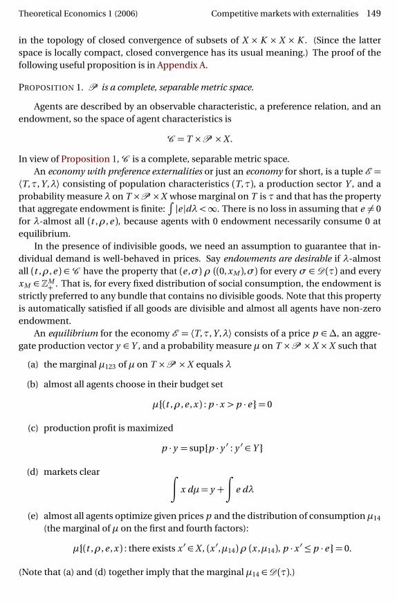
in the topology of closed convergence of subsets of X × K × X × K . (Since the latterspace is locally compact, closed convergence has its usual meaning.) The proof of thefollowing useful proposition is in Appendix A.

PROPOSITION 1. P is a complete, separable metric space.

Agents are described by an observable characteristic, a preference relation, and anendowment, so the space of agent characteristics is

C = T ×P ×X .

In view of Proposition 1,C is a complete, separable metric space.An economy with preference externalities or just an economy for short, is a tuple E =

⟨T,τ, Y ,λ⟩ consisting of population characteristics (T,τ), a production sector Y , and aprobability measure λ on T ×P ×X whose marginal on T is τ and that has the propertythat aggregate endowment is finite:

∫

|e |dλ<∞. There is no loss in assuming that e 6= 0for λ-almost all (t ,ρ, e ), because agents with 0 endowment necessarily consume 0 atequilibrium.

In the presence of indivisible goods, we need an assumption to guarantee that in-dividual demand is well-behaved in prices. Say endowments are desirable if λ-almostall (t ,ρ, e ) ∈ C have the property that (e ,σ) ρ ((0,xM ),σ) for every σ ∈ D (τ) and everyxM ∈ ZM

+ . That is, for every fixed distribution of social consumption, the endowment isstrictly preferred to any bundle that contains no divisible goods. Note that this propertyis automatically satisfied if all goods are divisible and almost all agents have non-zeroendowment.

An equilibrium for the economy E = ⟨T,τ, Y ,λ⟩ consists of a price p ∈ ∆, an aggre-gate production vector y ∈ Y , and a probability measure µ on T ×P ×X ×X such that

(a) the marginal µ123 of µ on T ×P ×X equals λ

(b) almost all agents choose in their budget set

µ{(t ,ρ, e ,x ) : p ·x > p · e }= 0

(c) production profit is maximized

p · y = sup{p · y ′ : y ′ ∈ Y }

(d) markets clear∫

x dµ= y +

∫

e dλ

(e) almost all agents optimize given prices p and the distribution of consumption µ14

(the marginal of µ on the first and fourth factors):

µ{(t ,ρ, e ,x ) : there exists x ′ ∈X , (x ′,µ14)ρ (x ,µ14), p ·x ′ ≤ p · e }= 0.

(Note that (a) and (d) together imply that the marginal µ14 ∈D (τ).)

150 Noguchi and Zame Theoretical Economics 1 (2006)

3.1 Individualistic representations

The descriptions above are entirely in distributional terms, but a description in individ-ualistic terms is sometimes possible. We say that the economy E = ⟨T,τ, Y ,λ⟩ admits anindividualistic representation if there is a measurable function ϕ : T →P ×X such that

λ= (idT ,ϕ)∗(τ)

where idT is the identity map on T and (idT ,ϕ)∗(τ) is the direct image measure. If Eadmits an individualistic representation then the equilibrium p , y ,µ admits an individ-ualistic representation if in addition there is a measurable function f : T →X such that

µ= (idT ,ϕ, f )∗(τ).

Informally—but entirely correctly—E admits an individualistic representation exactlywhen almost all agents having the same observable characteristic have the same en-dowment and preferences, and an equilibrium p , y ,µ admits an individualistic repre-sentation if and only if all agents having the same observable characteristic choose thesame consumption bundle.

As we show in Section 5, there are economies that admit an individualistic represen-tation for which no equilibrium admits an individualistic representation.

3.2 Economies with finite support

We should offer a caveat about interpretation. An economy E = ⟨T,τ, Y ,λ⟩ for which τand λ have finite support should not be interpreted as an economy with a finite numberof agents, but rather as an economy with a finite number of types of agents. Theorems 1and 2 of Section 4 are able to guarantee existence of equilibria for such economies onlybecause our notion of equilibrium does not require agents having the same character-istics to choose the same consumption bundles.

4. EXISTENCE OF EQUILIBRIUM

For an economy E = ⟨T,τ, Y ,λ⟩, we say that all goods are available in the aggregate if

�

Y +

∫

e dλ

�

∩RL+M++ 6= ;.

That is, all goods are either represented in the endowment or can be produced.Our main result guarantees existence of equilibrium.

THEOREM 1. Every economy E = ⟨T,τ, Y ,λ⟩ for which endowments are desirable and allgoods are available in the aggregate admits an equilibrium.

As Example 3 shows, convexity of preferences is not enough to guarantee the exis-tence of an equilibrium with an individualistic representation, but strict convexity willdo.

Theoretical Economics 1 (2006) Competitive markets with externalities 151

THEOREM 2. If E = ⟨T,τ, Y ,λ⟩ is an economy that admits an individualistic representa-tion, M = 0 (so there are no indivisible goods), and λ-almost all agents have preferencesthat are strictly convex in own consumption, then every equilibrium for E admits an in-dividualistic representation.

5. EXAMPLES

In this section, we give a number of examples to illustrate the power and usefulness ofour approach and to contrast our results with the results of Noguchi (2005), Cornet andTopuzu (2005), and Balder (2003). For ease of exposition, we do not stray far from thesetting we have already discussed; the particular functional forms are chosen for ease ofcalculation, rather than for economic realism.

We begin by completing the discussion of Example 1.

EXAMPLE 1 CONTINUED. We begin by giving a distributional description of the economy.As before, all agents are endowed with one unit of each good: e = (1, 1). If σ ∈ D (τ) isthe distribution of consumption, an agent located at s ∈ [0, 1] who consumes (x1,x2)experiences the externality

η(s ,σ) =

∫

T×R2+

x dσ

and enjoys utility

u s (x2,x2,σ) = [2−η1(s ,σ)]x 21 +[2−η2(s ,σ)]x 2

2 .

Hence λ is the image of τ under the map s 7→ (s , u s , e ).The argument of Section 2 shows that, at equilibrium, we must have p1 = p2 = 1

2 andη1(s ,σ) = η2(s ,σ) for all s ∈ [0, 1]. This condition characterizes a unique equilibriumdistribution; to describe it, define maps g 1, g 2 : T → T ×P ×R2

+×R2+ by

g 1(s ) = (s , u s , (1, 1), (2, 0))

g 2(s ) = (s , u s , (1, 1), (0, 2)).

The unique equilibrium distribution is

µ= 12 g 1∗ (τ)+

12 g 2∗ (τ).

The interpretation is simple: in every measurable set of locations, half of the agentschoose (2, 0) and half of the agents choose (0, 2). Informally: half of the agents at eachlocation choose (2, 0) and half of the agents choose (0, 2). Even more informally: “everyother agent” chooses (2, 0) and “every other agent” chooses (0, 2). There is no measur-able function with this property; there is, as Mas-Colell (1984) writes, “a measurabilityproblem.”1 ◊

This example relies on non-convex preferences; as the following example shows,problems for individualistic representations can arise also from indivisible goods.

1The same point is made in Gretsky et al. (1992), and may also be familiar from the literature on the lawof large numbers with a continuum of random variables (Feldman and Gilles 1985, Judd 1985).

152 Noguchi and Zame Theoretical Economics 1 (2006)

EXAMPLE 2. Again, we consider a large number of agents living along a river. We con-tinue to identify locations (the observable characteristic) with the interval T = [0, 1] andassume the population is uniformly distributed along the river, so τ is Lebesgue mea-sure. There are two goods: good 1 is divisible and good 2 (speedboats) is indivisible, soindividual consumption sets are X = R+×Z+; write x = (x1,x2) for a typical consump-tion bundle.

Speedboats are produced by a constant returns to scale technology: 1 unit of theconsumption good produces 1 speedboat, so the production cone is

Y = {(y1, y2) : y2 ≤−y1}.

Agents are each endowed with 2 units of the consumption good but no speedboats.Agents care about the consumption good and about speedboats, but utility from

speedboats is subject to a congestion externality. Ifσ ∈D (τ) is the distribution of socialconsumption, the congestion externality experienced by an agent located at s ∈ (0, 1] is

η(s ,σ) =1

s

∫

T×X

1[0,s ](t )x2 dσ(t ,x1,x2).

(We leave η(0,σ) undefined.) Note that, so long as all speedboat consumptions arebounded by 2 (which they are at any individually rational consumption distribution)the externality experienced by s is just the average of speedboat consumption upstreamfrom s . The utility obtained by an agent located at s who consumes x1 units of the divis-ible good and x2 speedboats is

u s (x1,x2;σ) = (x1)1/2�

1+2[x2−η(s ,σ)]+�1/2 .

Note that the externality matters only when speedboat consumption is strictly positive.2

To solve for equilibrium p , y ,µ normalize so that p1 = 1. Profit maximization entailsthat p2 ≤ 1 (else potential profit would be infinite). If no speedboats are produced thenthe equilibrium must be autarkic: every agent consumes his/her endowment (2, 0) andobtains utility 21/2. However, if no speedboats are produced then no agent experiences acongestion externality, and each agent prefers to consume (1, 1) and obtain utility 31/2 >

21/2. Hence speedboats must be produced at equilibrium, and now profit maximizationentails that in fact p2 = 1.

To solve for µ, write σ = µ14 for the marginal of µ on observable characteristicsand speedboat consumption. Because τ is non-atomic, η(t ,σ) is a continuous func-tion of t ; we claim that η(t ,σ) ≡ 1

2 for every t ∈ (0, 1]. To see this, consider the openset {s : E (s ,σ)< 1

2}. If this is not empty it is the countable union of disjoint intervals; letI be any one of these intervals, and let a be the left-hand endpoint of I . Check that ifη(s ,σ)< 1

2 then the unique optimal choice for an agent located at s is to consume (1, 1).Thus, if a = 0 then η(s ,σ)≡ 1 for every s ∈ I , which certainly contradicts the definitionof I . Hence a 6= 0, and a /∈ I (because I is open). Continuity therefore guarantees that

2This utility function is not strictly increasing in x2, but it is so in the relevant range.

Theoretical Economics 1 (2006) Competitive markets with externalities 153

η(a ,σ) = 12 , so that η(s ,σ) is a strictly increasing function of I ; in particular, η(s ,σ)> 1

2for each s ∈ I , which again contradicts the definition of I . Since we have reached a con-tradiction whether or not a = 0, we conclude that {s : E (s ,σ)< 1

2} is empty. Similarly, wesee that {s : E (s ,σ)> 1

2} is empty, so E (s ,σ)≡ 12 for every s ∈ (0, 1].

It follows immediately that equilibrium production is y = (− 12 ,+ 1

2 ).If equilibrium had an individualistic representation then there would be a function

f = ( f 1, f 2) : T →R+×Z+ for which

1

s

∫ s

0

f 2(t )dτ(t ) = 12

for each s —but no such integer-valued function exists.To define the unique equilibrium consumption distribution, define g 1, g 2 : T → T ×

P ×X ×X by

g 1(s ) = (s , u s , (2, 0), (2, 0))

g 2(s ) = (s , u s , (2, 0), (1, 1)).

The unique equilibrium distribution is

µ= 12 g 1∗ (τ)+

12 g 2∗ (τ).

That is: at every location half of the agents consume their endowments and half of theagents use one unit of consumption to produce one speedboat. ◊

Examples 1 and 2 provide useful comparisons with Balder (2003), Noguchi (2005)and Cornet and Topuzu (2005). Balder assumes that the externality enters into eachagent’s utility function in the same way. This would only be the case if pollution (inExample 1) and congestion (in Example 2) had the same negative effects upstream asdownstream. More generally, this assumption would obtain only for externalities thatare purely global—but few, if any, externalities would seem to have this property. (Evena negative externality as wide-spread as global warming affects different regions of theearth in different ways.)

Noguchi (2005) and Cornet and Topuzu (2005) assume that individual preferencesare convex. As we have discussed, this assumption is problematic in a continuum econ-omy, and especially so in the presence of externalities. As Examples 1 and 2 demon-strate, if preferences are non-convex or some goods are indivisible, an individualisticequilibrium may not exist—but our distributional framework handles non-convex pref-erences and indivisible goods smoothly.

A more subtle point concerns the nature of the externality. Noguchi (2005) and Cor-net and Topuzu (2005) assume that the externality experienced by each agent is contin-uous with respect to the topology of weak convergence of consumption allocations. If,as in Examples 1 and 2, the externality experienced by an agent is of the form

η( f ) =

∫

T

E ( f (t ))dt ,

154 Noguchi and Zame Theoretical Economics 1 (2006)

weak continuity in f obtains only if E is linear (more precisely, affine) on the relevantrange. This is evidently a strong assumption. In our framework, the corresponding ex-ternality is

η(σ) =

∫

T×X

E (t ,x )dσ(t ,x )

and our requirement that preferences be continuous with respect to the topology ofweak convergence of distributions is satisfied if E is measurable, bounded (or just uni-formly integrable on the relevant range of distributions inD (τ)), and continuous in x . Asthe following simple example demonstrates, non-linear externalities are a problem forthe individualistic approach but are handled smoothly in our distributional approach.

EXAMPLE 3. Again, T = [0, 1] and τ is Lebesgue measure. There are two goods, bothdivisible. When the distribution of consumption is σ ∈ Prob(T ×R2

+), an agent locatedat s ∈ T who chooses the bundle (x1,x2) experiences the externality

η(s ,σ) =

∫

T×R2+

1[0,s ](t )(x1x2+x1−x2)dσ(t ,x1,x2)

and enjoys the utility

u s (x1,x2;σ) = x1+(1+η(s ,σ))x2.

All agents are endowed with one unit of each good: e = (1, 1). There is no production:Y =−R2

+.To solve for equilibrium p ,µ we follow a by-now-familiar strategy. Consider the dis-

joint open sets

W1 =�

t ∈ T :1

p1>

1+η(t ,σ)p2

�

W2 =�

t ∈ T :1

p1<

1+η(t ,σ)p2

�

.

If s ∈W1 then every agent located at s strictly prefers to consume only good 1, so η(·,σ)is strictly increasing on every subinterval of W1. If s ∈W2 then every agent located at sstrictly prefers to consume only good 2, so η(·,σ) is strictly increasing on every subin-terval of W2. Arguing just as in the previous two examples, this quickly leads to a contra-diction unless W1 =W2 = ;.

We conclude that1

p1=

1+η(s ,σ)p2

for every s ∈ T . In particular, η(·,σ) is constant. Since η(0,σ) = 0 it follows that η(·,σ)≡

Theoretical Economics 1 (2006) Competitive markets with externalities 155

0. Since total endowments are (1, 1)we have

0=η(1,σ) =

∫

T×R2+

1(x1x2+x1−x2)dσ(t ,x1,x2)

=

∫

T×R2+

(x1x2)dσ(t ,x1,x2)+

∫

T×R2+

(x1−x2)dσ(t ,x1,x2)

=

∫

T×R2+

(x1x2)dσ(t ,x1,x2).

Because consumption is non-negative, this implies x1x2 = 0 almost everywhere withrespect toσ: no agent consumes both goods. Given that endowments are (1, 1) it followsthat the unique equilibrium price is p1 = p2 = 1

2 and the unique equilibrium distributionis

µ= 12 g 1∗ (τ)+

12 g 2∗ (τ)

where g 1, g 2 : T → T ×P ×X ×X are defined by

g 1(s ) = (s , u s , (1, 1), (2, 0))

g 2(s ) = (s , u s , (1, 1), (0, 2)).

Informally: at each location, half the agents choose (2, 0) and half the agents choose(0, 2). As before, this equilibrium does not admit an individualistic representation. ◊

We conclude with an example that illustrates that our distributional framework, al-though perhaps less familiar than the individualistic framework, is just as useful.

EXAMPLE 4. It is natural to conjecture that negative externalities lead to sub-optimalequilibria; we verify that conjecture in a particular setting. (It is sometimes said thatnegative externalities invariably lead to sub-optimal equilibria; as we shall see, this isnot so.)

We consider a more general environment than above. Let T ⊂ R2 be a compactset, and let τ be a probability measure on T with full support. We identify T as a setof locations (a city or neighborhood) and τ as the (relative) population density. (Theassumption of full support means there are no unpopulated areas.)

For notational simplicity, assume that there are only two goods, both divisible, thatall agents are endowed with one unit of the first good but that the second good mustbe produced.3 One unit of the second good can be produced from one unit of the firstgood, so the production cone is:

Y = {(y1, y2) : y1 ≤ 0, y2 ≤−y1}.

If the distribution of consumption isσ ∈ Prob(T ×R2+), an agent located at s ∈ T experi-

ences the externality

η(s ,σ) =

∫

T×R2+

E (s , t ,x )dσ(t ,x ).

3More general specifications would add only notational complication.

156 Noguchi and Zame Theoretical Economics 1 (2006)

If the agent consumes consumes the bundle (x1,x2) she enjoys utility

u s (x1,x2,σ) =U (s ,x1,x2,η(s ,σ)).

For simplicity, assume E is real-valued. To guarantee that preferences satisfy the re-quirements of Theorem 1 and hence that an equilibrium exist, it suffices to assume thatE is measurable, uniformly integrable on eachDn (τ) (boundedness would be enough),and continuous in x , and that U is measurable, continuous in x1, x2, η, and strictly in-creasing in x1, x2.

Assume the derivatives of E and U obey

∂ E

∂ x1= 0,

∂ E

∂ x2> 0,

∂U

∂ x i> 0 for i = 1, 2

∂U

∂ η(s ,x1,x2,η)< 0 if x2 > 0.

That is: only good 2 causes pollution, pollution at location s from consumption at lo-cation t is strictly increasing in consumption of good 2, utility is strictly increasing inconsumption and strictly decreasing in experienced pollution.

These assumptions do not guarantee that equilibrium is inefficient. For example,suppose there are only two locations, so T = {s1, s2}, and that half the population livesat each location. Consumption of x2 at any location creates an equal externality at everylocation

η(s ,σ) =

∫

T×R2+

x2 dσ.

Utility functions for agents who live at s1 are

u 1(x1,x2,η) = x1+(3−η)x2

while utility functions for agents who live at s2 are

u 2(x1,x2,η) = x1+(1−η)x2.

One equilibrium for this economy can be described in the following way: prices arep1 = p2 = 1

2 ; agents who live at s1 consume (0, 1) and agents who live at s2 consume(1, 0). This equilibrium is efficient. The point is one made by Starrett (1972): agents at s2

escape the negative effects of pollution by not consuming the second good at all.However, these assumptions do guarantee that any equilibrium in which some

agents consume both goods must be inefficient; in any such equilibrium, good 2 is over-produced.4 To see this, let p , y ,µ be an equilibrium in which some agents consume bothgoods, and let σ be the marginal of µ on T ×R2

+ (the distribution of locations and con-sumption). Because good 2 is produced, profit maximization entails that prices of goods1, 2 must be equal: p1 = p2. Let

B1 = {(s , u s , e ,x ) : x1 > 0,x2 > 0}.4We could guarantee that some agents consume both goods by requiring that marginal utilities of con-

sumption at 0 be infinite.

Theoretical Economics 1 (2006) Competitive markets with externalities 157

By assumption, µ(B1) > 0. For (s , u s , e ,x ) ∈ B1 and ε > 0 small, set x ε = (x1+ ε,x2− ε).Our differentiability assumptions imply that

limε→0

�

�

�

�

u s (x ε ,σ)−u s (x ,σ)ε

�

�

�

�

= 0 (1)

limε→0

�

E (s , t ,x ε)−E (s , t ,x )ε

�

> 0. (2)

A straightforward measure-theoretic argument shows that there is a subset B2 ⊂ B1

such that for (s , u s , e ,x ), (t , u t , e ,x ) ∈ B2 convergence of the limits in (1) and (2) is uni-form, the limit in (2) is bounded away from 0, and consumption of good 2 is boundedaway from 0. Write B c

2 for the complement of B2, define h : B2 → B2 by h(s , u s , e ,x ) =(s , u s , e ,x ε), and set

µ=µ|B c2+h∗(µ|B2 )

Thus µ and µ differ only in that agents who were initially in B2 consume slightly moreof good 1 and slightly less of good 2. If ε is small enough, these agents are better offbecause the loss in shifting own consumption x to x ε (which is of order less than ε) ismore than offset by the reduction in the externality (which is of order ε). In particular, µis not Pareto optimal. ◊

APPENDIX

A. PROOFS

We first isolate a useful lemma, then verify Proposition 1.

LEMMA. Every compact subset of D (τ) is contained in some Dn (τ).

PROOF. Suppose this is not true, so that there is a compact set K ⊂D (τ) and for each nthere is a measure σn ∈ K ,σn /∈ Dn (τ); there is no loss assuming that σn ’s are distinct.If E is any subset of S = {σn : n = 1, . . .} then for each m ,

E ∩Dm (τ)⊂S ∩Dm (τ)⊂ {σn : n = 1, . . . , m −1}

so E ∩Dm (τ) is finite, hence closed. By definition of the direct limit topology, therefore,E is a closed subset of D (τ). Because E is arbitrary, this means that every subset ofS is closed; i.e., S is a discrete set. On the other hand, compactness of K implies that{σn : n = 1, . . .} is compact. This is a contradiction, so we conclude that every compactsubset ofD (τ) is contained in someDn (τ), as asserted. �

PROOF OF PROPOSITION 1. Let P0 be the space of preference relations that are open,irreflexive, transitive and negatively transitive in own consumption (but not necessarilymonotone). We first define a complete metric on P0. To this end, fix, for each n , acomplete metric d n on the space C n of closed subsets of X ×Dn (τ)× X ×Dn (τ). For

158 Noguchi and Zame Theoretical Economics 1 (2006)

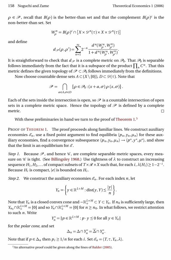
ρ ∈ P , recall that B (ρ) is the better-than set and that the complement B (ρ)c is thenon-better-than set. Set

W nρ = B (ρ)c ∩�

X ×Dn (τ)×X ×Dn (τ)�

and define

dP (ρ,ρ′) =∞∑

n=1

2−nd n (W n

ρ , W nρ′ )

1+d n (W nρ , W n

ρ′ ).

It is straightforward to check that dP is a complete metric on P0. That P0 is separablefollows immediately from the fact that it is a subspace of the product

∏

n C n . That thismetric defines the given topology ofP ⊂P0 follows immediately from the definitions.

Now choose countable dense sets A ⊂ (X \ {0}), D ⊂D (τ). Note that

P =⋂

a∈A,σ∈D

�

ρ ∈P0 : (x +a ,σ)ρ (x ,σ)

.

Each of the sets inside the intersection is open, soP is a countable intersection of opensets in a complete metric space. Hence the topology of P is defined by a completemetric. �

With these preliminaries in hand we turn to the proof of Theorem 1.5

PROOF OF THEOREM 1. The proof proceeds along familiar lines. We construct auxiliaryeconomies En , use a fixed point argument to find equilibria ⟨pn , yn ,µn ⟩ for these aux-iliary economies, find a convergence subsequence ⟨pn , yn ,µn ⟩ → ⟨p ∗, y ∗,µ∗⟩, and showthat the limit is an equilibrium for E .

Step 1. Because P , and hence C , are complete separable metric spaces, every mea-sure on C is tight. (See Billingsley 1968.) Use tightness of λ to construct an increasingsequence H1, H2, . . . of compact subsets of T×R×X such that, for each i ,λ(Hi )≥ 1−2−i .Because Hi is compact, |e | is bounded on Hi .

Step 2. We construct the auxiliary economies En . For each index n , let

Yn =�

y ∈RL+M : dist(y , Y )≤|y |n

�

.

Note that Yn is a closed convex cone and−RL+M+ ⊂ Y ⊂ Yn . If n 0 is sufficiently large, then

Yn 0∩RL+M+ = {0} and so Yn ∩RL+M

+ = {0} for n ≥ n 0. In what follows, we restrict attentionto such n . Write

Y ◦n = {p ∈RL+M : p · y ≤ 0 for all y ∈ Yn}

for the polar cone, and set∆n =∆∩Y ◦n =∆∩Y ◦n .

Note that if p ∈∆n then p i ≥ 1/n for each i . Set En = ⟨T,τ, Yn ,λ⟩.5An alternative proof could be given along the lines of Balder (2005).

Theoretical Economics 1 (2006) Competitive markets with externalities 159

Step 3. Fix n . We construct compact convex spaces of prices and consumption distri-butions, and a correspondence on the space of prices and consumption distributions.

Set

Kn = {(t ,ρ, e ,x )∈C ×X : |x | ≤ Ln |e |}Kn = {µ∈ Prob(C ×X ) :µC =τ, and µ(Kn ) = 1}

where µC is the marginal of µ on C . It is evident thatKn is a closed subset of Prob(C ×X ), and tightness of λ entails thatKn is tight, soKn is weakly compact. (See Billingsley1968.) To see thatKn is non-empty, write

proj :C ×X →C

for the projection. For B ⊂C ×X a Borel set, write

B0 = B ∩ (C ×{0}) .

Define the probability measure µ by µ(B ) = λ�

proj(B0)�

; note that µ ∈ Kn , so Kn isnon-empty.

We define a correspondence Φn on∆n ×Kn as the product of correspondences

φn :∆n ×Kn →Kn

ψn :∆n ×Kn →∆n .

Given (t ,ρ, e ) ∈ T ×P ×X = C , p ∈ ∆n and µ ∈ Prob(C ×X ) having the property thatµ14 ∈ D (τ) (recall that µ14 is the marginal of µ on observable characteristics and con-sumptions), define individual budget and demand sets by:

B (t ,ρ, e ;µ, p ) = {x ∈X : p ·x ≤ p · e }d (t ,ρ, e ;µ, p ) = {x ∈ B (t ,ρ, e ;µ, p ) : (x ′,µ14)ρ (x ,µ14)⇒ p ·x ′ > p · e }.

Note that if p ∈∆n then

d (t ,ρ, e ;µ, p )⊂ B (t ,ρ, e ;µ, p )⊂ Kn .

Finally, let D(µ, p ) be the set of agents who choose in their demand set:

D(µ, p ) = {(t ,ρ, e ,x ) : x ∈ d (t , R , e ;µ, p )}.

Now define the required correspondences by

φn (p ,µ) = {ν ∈Kn : ν (D(µ, p )) = 1}

ψn (p ,µ) = argmax

¨

q ·�∫

x dµ−∫

e dµ

�

: q ∈∆n

«

Φn (p ,µ) =ψn (p ,µ)×φn (p ,µ).

160 Noguchi and Zame Theoretical Economics 1 (2006)

Step 4. We claim thatφn ,ψn ,Φn are upper-hemi-continuous, and have compact, con-vex, non-empty values.

It is evident that φn has convex values. To show that it is upper-hemi-continuous,we first show that the individual demand is closed. To this end, let (t ,ρ, e ) ∈ C , letx j ∈ d (t ,ρ, e ;µj , p j ) and suppose x j → x ; we must show x ∈ d (t ,ρ, e ;µ, p ). Writex = (xL ,xM ) where xL ∈ RL

+ and xM ∈ ZM+ . Because endowments are desirable, xL 6= 0,

else (e ,µ14) ρ (x ,µ14) and x would not be in the demand set. Hence p · (xL , 0) > 0 andp · ((1−ε)xL ,xM )< p ·x for every ε> 0. It then follows by a familiar continuity argumentthat x ∈ d (t ,ρ, e ;µ, p ), as desired

Because ∆n ,Kn are compact, to see that φn is upper-hemi-continuous and hascompact values, it suffices to show that it has closed graph. To this end, let {(p j ,µj )}be a sequence in ∆n ×Kn converging to (p ,µ); for each j , let ν j ∈ φn (p j ,µj ) and as-sume ν j → ν ; we must show ν ∈φn (p ,µ). For each i , writeHi =Hi ×X . By definition,ν j [D(µj , p j )] = 1, so

ν j [D(µj , p j )∩Hi ]≥ 1−2−i .

Convergence of ν j to ν implies that

ν

�

lim supj→∞

�

D(µj , p j )∩Hi

�

�

≥ 1−2−i .

On the other hand, it follows from closedness of the individual demand correspondencethat

D(µ, p )∩Hi ⊃ lim supj→∞

�

D(µj , p j )∩Hi

�

so that ν [D(µ, p ) ∩Hi ] ≥ 1− 2−i . Since i is arbitrary, it follows that ν [D(µ, p )] = 1 soν ∈φn (p ,µ), as desired. Henceφn is upper-hemi-continuous.

To see thatφn has non-empty values, fix (p ,µ). For each (t ,ρ, e ), let f (t ,ρ, e ) be theunique lexicographically smallest element of d (t ,ρ, e ,µ, p ). It is easily checked that f isa measurable function, and that the direct image measure f ∗λ belongs toφn (p ,µ).

That ψn is upper-hemi-continuous, and has compact, convex, non-empty valuesfollows immediately from the usual argument for Berge’s Maximum Theorem.

Finally, Φn is upper-hemi-continuous, and has compact, convex, non-empty valuesbecauseφn ,ψn enjoy these properties.

Step 5. Because ∆n , Kn are compact and convex and Φn is upper-hemi-continuousand has compact, convex, non-empty values, Φn has a fixed point (pn ,µn ). Set yn =∫

x dµn −∫

e dλ. We claim that ⟨pn , yn ,µn ⟩ constitutes an equilibrium for the economyEn .

The construction guarantees that almost all agents optimize in their budget sets. Bydefinition, pn maximizes the value of yn , which is aggregate excess demand at pn ,µn .Walras’s Law guarantees that the value of excess demand at pn ,µn is 0: pn · yn = 0. Ifyn 6∈ Yn there would be a price p ∈ Y ◦n such that p ·yn > 0. However this would contradictthe fact that pn maximizes the value of excess demand. Hence yn ∈ Yn . By construction,pn ∈ Y ◦n , so pn · y ≤ 0 for every y ∈ Yn ; this is profit maximization. Hence ⟨pn , yn ,µn ⟩constitutes an equilibrium for the economy En .

Theoretical Economics 1 (2006) Competitive markets with externalities 161

Step 6. We show that the equilibria ⟨pn , yn ,µn ⟩ lie in compact sets of prices, productionvectors, and distributions.

Note first that all prices pn lie in∆, which is compact. By construction, yn =∫

x dµn−∫

e dλ so y −n ≤∫

e dλ. Because there is no free production (Yn 0 ∩RL+M+ = {0}), rates of

transformation are bounded. Hence there is some constant A such that if y ∈ Yn 0 thenthe positive and negative parts of y satisfy the inequality |y +| ≤ A |y −|. Thus y −n ≤

∫

e dλand

|y +n | ≤ A |y −n | ≤ A

�

�

�

�

∫

e dλ

�

�

�

�

. (3)

Hence, the production vectors yn lie in a bounded subset of RL+M .To see that the distributions µn lie in a tight (hence relatively compact) set, recall the

sets Hi constructed in Step 1. Fix i . For each k set

Gk = {(t , R , e ,x )∈Hi ×X : |x | ≤ k }Jk = {(t , R , e ,x )∈Hi ×X : |x |> k }.

For each n∫

Jk

|x |dµn ≥ k µn (Jk ). (4)

By construction,∫

x dµn = yn +

∫

e dλ ≤ y +n +

∫

e dλ.

In view of (3), this implies∫

|x |dµn =

�

�

�

�

∫

x dµn

�

�

�

�

≤ (1+A)

�

�

�

�

∫

e dλ

�

�

�

�

. (5)

Combining (4) and (5) we conclude that

µn (Jk )≤(1+A)

k

�

�

�

�

∫

e dλ

�

�

�

�

.

Choose k large enough so that the right hand side is smaller than 2−i . Since Gk ∪ Jk =Hi ×X and µn (Hi ×X ) = λ(Hi )≥ 1− 2−i , it follows that µn (Gk )> 1− 2−i+1. Because Gk

is compact, we conclude that {µn} is a uniformly tight family, hence relatively compact.We conclude that prices pn , production vectors yn , and consumption distributions µn

lie in compact sets, as asserted.

Step 7. Some subsequence of ⟨pn , yn ,µn ⟩ converges; say

⟨pn , yn ,µn ⟩→ ⟨p ∗, y ∗,µ∗⟩.

By construction, Y =⋂

Yn . Since pn ∈ ∆ ∩ Y ◦n and yn ∈ Yn for each n , it follows thatp ∗ ∈∆∩Y ◦ and y ∗ ∈ Y . We claim that p ∗ ∈∆ and that ⟨p ∗, y ∗,µ∗⟩ is an equilibrium for E .

To see that p ∗ ∈∆, suppose not; say p ∗j = 0. We distinguish two cases, and obtain acontradiction in each case.

162 Noguchi and Zame Theoretical Economics 1 (2006)

Case 1: p ∗ ·∫

e dλ= 0. Because p ∗ 6= 0 and all goods are available in the aggregate, thereis some x ∈ RL+M

+ such that p ∗ · x > 0 and�

x −∫

e dλ�

∈ Y . Thus, p ∗ ·�

x −∫

e dλ�

> 0.Since p ∗ ∈ Y ◦, we have a contradiction.

Case 2: p ∗ ·∫

e dλ > 0. Then there is some ` such that p ∗` > 0 and∫

e`dλ > 0. LetE = {(t ,ρ, e ) : e` > 0}. Because

∫

e`dλ > 0 it follows that λ(E ) > 0. Because λ is regularand tight, it follows that there is a compact set J ⊂ E such that λ(J )> 0. Define

Z =�

ν ∈ Prob(C ×X ) : νC =λ,

∫

|x |dν ≤ (1+A)

∫

|e |dλ�

.

Arguing as before shows that Z is weakly closed and uniformly tight, hence weaklycompact.

We claim that as n →∞ aggregate demand is uniformly unbounded on Z : for everyα> 0 there is an integer n 0 such that if n ≥ n 0, (t ,ρ, e )∈ J , ν ∈Z , and z ∈ d (t ,ρ, e ;ζ, pn )then |z | > α. To see this, suppose not. Then there is some α > 0 such that for every n 0

there is some n > n 0, some (t ,ρ, e ) ∈ J , some ζ ∈Z , and some z n ∈ d (t ,ρ, e ;ζ, pn ) suchthat |z n | ≤α. Letting n 0 tend to infinity, passing to limits of subsequences where neces-sary, and recalling the definition of the topology of P , that J , Z are compact, and thatpreference relations are continuous in the distribution of consumption, and arguing asin Step 4, we find (t ∗,ρ∗, e ∗) ∈ Z , ν∗ ∈ J and z ∗ ∈ d (t ∗,ρ∗, e ∗;ν∗, p ∗) such that |z ∗| ≤ α.Because p ∗ ·e ∗ > 0, p ∗j = 0 and ρ∗ is strictly monotone, this is absurd. This contradictionestablishes the claim.

Now apply the claim with α = 2�

�

∫

e dλ�

�/λ(J ) to conclude that there is an n 0 suchthat for every (t ,ρ, e )∈ J , each n ≥ n 0 and every z ∈ d (t ,ρ, e ;ν , pn )we have

|z |> 2

�

�

�

�

∫

e dλ

�

�

�

�

/λ(J ).

If follows in particular that∫

J

inf{|z | : z ∈ d (t ,ρ, e ;µn , pn )}dλ≥ 2

�

�

�

�

∫

e dλ

�

�

�

�

for each n . However, as we have shown above,∫

|x |dµn ≤�

�

�

�

∫

e dλ

�

�

�

�

so we have a contradiction.

Since we obtain contradictions in each case, we conclude that p ∗ ∈∆, as asserted.Arguing as in Step 4 shows that µ∗[D(µ∗, p ∗)] = 1 and that

∫

x dµ∗ = y ∗ +∫

e dλ, so⟨p ∗, y ∗,µ∗⟩ is an equilibrium for E . The proof is complete. �

PROOF OF THEOREM 2. Let p , y ,µ be an equilibrium. Strict convexity of preferencesguarantees that λ-almost all agents have unique demands at the given price p and dis-tribution µ. Put differently, for almost all (t ,ρ, e ), the demand set d (t ,ρ, e ,µ, p ) is a sin-gleton. By assumption, E has an individualistic representation, so there is a measurableϕ : T →P ×X such that λ= (idT ,ϕ)∗(τ). Define f : T →X by

f (t ) = d (t ,ϕ(t ),µ, p ).

Theoretical Economics 1 (2006) Competitive markets with externalities 163

It is easily checked that f is measurable and that

µ= (idT ,ϕ, f )∗(τ)

so p , y ,µ admits an individualistic representation, as asserted. �

B. EXTERNALITIES AS A PARAMETER

An alternative formulation of externalities in preferences has the distribution of con-sumption entering as a parameter. Here we give a brief sketch of this alternative. Com-modities, consumption sets, production, and the distribution of consumption are all asin Section 3.

As in Hildenbrand (1974), write P ∗mo for the space of continuous, irreflexive, tran-sitive, negatively transitive, strictly monotone preference relations on X ; in the topol-ogy of closed convergence, P ∗mo is a complete separable metric space. We define aparametrized preference to be a map

R :D (τ)→P ∗mo .

We write x R(σ) y to mean that the consumption bundle x is preferred to the consump-tion bundle y when σ is the distribution of consumption. The preference relation R iscontinuous if the set

{(x , y ,σ)∈X ×X ×D (τ) : x R(σ) y }

is open. The following proposition records that continuity of the preference relation Ris equivalent to continuity of R as a mapping.

PROPOSITION 2. For a parametrized preference relation R the following are equivalent.

(i) R is continuous as a preference relation (in the sense above).

(ii) The mapping R :D (τ)→P ∗mo is continuous.

(iii) For each n the restriction R :Dn (τ)→P ∗mo is continuous.

WriteR for the space of continuous parametrized preference relations, and giveRthe topology of uniform convergence on compact subsets ofD (τ). The following can beproved by combining the Lemma of Appendix A together with Proposition 2.

PROPOSITION 3. R is a complete, separable metric space.

Agents are characterized by an observable characteristic, a preference relation, andan endowment, so for this description of preferences, the space of agent characteristicsis

CP = T ×R ×X .

In view of Proposition 3,CP is a complete separable metric space.

164 Noguchi and Zame Theoretical Economics 1 (2006)

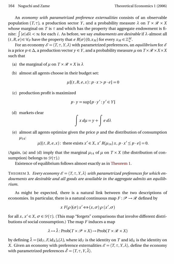
An economy with parametrized preference externalities consists of an observablepopulation (T,τ), a production sector Y , and a probability measure λ on T ×R × Xwhose marginal on T is τ and which has the property that aggregate endowment is fi-nite:∫

|e |dλ <∞ for each i . As before, we say endowments are desirable if λ-almost all(t , R , e )∈CP have the property that e R(σ) (0,xM ) for every xM ∈ZM

+ .For an economy E = ⟨T,τ, Y ,λ⟩with parametrized preferences, an equilibrium for E

is a price p ∈∆, a production vector y ∈ Y , and a probability measureµ on T×R×X×Xsuch that

(a) the marginal of µ on T ×R ×X is λ

(b) almost all agents choose in their budget set:

µ{(t , R , e ,x ) : p ·x > p · e }= 0

(c) production profit is maximized

p · y = sup{p · y ′ : y ′ ∈ Y }

(d) markets clear∫

x dµ= y +

∫

e dλ

(e) almost all agents optimize given the price p and the distribution of consumptionµ14:

µ{(t , R , e ,x ) : there exists x ′ ∈X , x ′ R(µ14) x , p ·x ′ ≤ p · e }= 0.

(Again, (a) and (d) imply that the marginal µ14 of µ on T × X (the distribution of con-sumption) belongs toD (τ).)

Existence of equilibrium follows almost exactly as in Theorem 1.

THEOREM 3. Every economy E = ⟨T,τ, Y ,λ⟩ with parametrized preferences for which en-dowments are desirable and all goods are available in the aggregate admits an equilib-rium.

As might be expected, there is a natural link between the two descriptions ofeconomies. In particular, there is a natural continuous map F :P →R defined by

x F (ρ)(σ) x ′⇔ (x ,σ)ρ (x ′,σ)

for all x , x ′ ∈ X ,σ ∈D (τ). (This map “forgets” comparisons that involve different distri-butions of social consumption.) The map F induces a map

λ 7→ λ : Prob(T ×P ×X )→ Prob(T ×R ×X )

by defining λ= (idT , F, idX )∗(λ), where idT is the identity on T and idX is the identity onX . Given an economy with preference externalities E = ⟨T,τ, Y ,λ⟩, define the economywith parametrized preferences E = ⟨T,τ, Y , λ⟩.

Theoretical Economics 1 (2006) Competitive markets with externalities 165

THEOREM 4. If E = ⟨T,τ, Y ,λ⟩ is an economy with preference externalities, then E and Ehave the same equilibrium prices and production plans.6

PROOF. Given µ∈ Prob(T ×P ×X ×X ), define

µ= (idT , F, idX , idX )∗(µ)∈ Prob(T ×R ×X ×X ).

It is straightforward to check that if E is an economy with preference externalities andp , y ,µ is an equilibrium for E then p , y , µ is an equilibrium for E .

All that remains is to show that if p , y ,ν is an equilibrium for E , then we can find anequilibrium p , y ,µ for E such that ν = µ. To this end, use disintegration of measures tofind a measurable map

ξ : T ×R ×X → Prob(X )

such that

ν =

∫

T×R×X

ξ(t , R , e )dλ.

Set

µ=

∫

T×P ×X

ξ(t , F (ρ), e )dλ

and check that p , y ,µ is an equilibrium for E and that µ= ν . �

REFERENCES

Aumann, Robert J. (1964), “Markets with a continuum of traders.” Econometrica, 32, 39–50. [144]

Aumann, Robert J. (1966), “Existence of competitive equilibrium in markets with a con-tinuum of traders.” Econometrica, 34, 1–17. [144]

Balder, Erik (2003), “Existence of competitive equilibria in economies with a mea-sure space of consumers and consumption externalities.” Working Paper, University ofUtrecht. [144, 151, 153]

Balder, Erik (2005), “More about equilibrium distributions for competitive markets withexternalities.” Working Paper, University of Utrecht. [158]

Billingsley, Patrick (1968), Convergence of Probability Measures. John Wiley and Sons,New York. [158, 159]

Cornet, Bernard and Mihaela Topuzu (2005), “Existence of equilibria for economies withexternalities and a measure space of consumers.” Economic Theory, 26, 397–421. [144,151, 153]

6We do not claim that E and E have the same equilibrium consumption distributions. The problem isthat F is not one-to-one, so many characteristics inC may correspond to the same characteristic inCP .

166 Noguchi and Zame Theoretical Economics 1 (2006)

Feldman, Mark and Christian Gilles (1985), “An expository note on individual risk with-out aggregate uncertainty.” Journal of Economic Theory, 35, 26–32. [151]

Gretsky, Neil E., Joseph M. Ostroy, and William R. Zame (1992), “The nonatomic assign-ment model.” Economic Theory, 2, 103–127. [151]

Hammond, Peter J., Mamoru Kaneko, and Myrna Holtz Wooders (1989), “Continuumeconomies with finite coalitions: Core, equilibria, and widespread externalities.” Journalof Economic Theory, 49, 113–134. [144]

Hart, Sergiu, Werner Hildenbrand, and Elon Kohlberg (1974), “On equilibrium alloca-tions as distributions on the commodity space.” Journal of Mathematical Economics, 1,159–166. [144]

Hildenbrand, Werner (1974), Core and Equilibria of a Large Economy. Princeton Univer-sity Press, Princeton. [163]

Judd, Kenneth L. (1985), “The law of large numbers with a continuum of IID randomvariables.” Journal of Economic Theory, 35, 19–25. [151]

Laffont, Jean-Jacques (1977), Effets Externes et Théorie Économique. Éditions du CentreNational de la Recherche Scientifique, Paris. [143]

Mas-Colell, Andreu (1984), “On a theorem of Schmeidler.” Journal of Mathematical Eco-nomics, 13, 201–206. [148, 151]

McKenzie, Lionel W. (1959), “On the existence of general equilibrium for a competitivemarket.” Econometrica, 27, 54–71. [147]

Noguchi, Mitsunori (2005), “Interdependent preferences with a continuum of agents.”Journal of Mathematical Economics, 41, 665–686. [144, 151, 153]

Shafer, Wayne and Hugo Sonnenschein (1975), “Equilibrium in abstract economieswithout ordered preferences.” Journal of Mathematical Economics, 2, 345–348. [143]

Starrett, David A. (1972), “Fundamental nonconvexities in the theory of externalities.”Journal of Economic Theory, 4, 180–199. [143, 156]

Submitted 2004-12-27. Final version accepted 2005-10-31. Available online 2005-12-2.