Identification and Estimation of Outcome Response with Heterogeneous Treatment Externalities

W O R K I N G P A P E R S E R I E S

TH

E M

AX

WE

LL

SC

HO

OL

C E N T E R F O R P O L I C Y R E S E A R C H

Tiziano Arduini, Eleonora Patacchini, and Edoardo Rainone

http://www.maxwell.syr.edu/CPR_Working_Papers.aspx

426 Eggers Hall

Syracuse University

Syracuse, NY 13244-1020

(315) 443-3114 / email: [email protected]

I S S N : 1 5 2 5 - 3 0 6 6

Paper No. 167 April 2014

CENTER FOR POLICY RESEARCH – Spring 2014

Leonard M. Lopoo, Director Associate Professor of Public Administration and International Affairs (PAIA)

__________

Associate Directors

Margaret Austin Associate Director

Budget and Administration

John Yinger Professor of Economics and PAIA

Associate Director, Metropolitan Studies Program

SENIOR RESEARCH ASSOCIATES

Badi H. Baltagi ............................................ Economics Robert Bifulco ....................................................... PAIA Thomas Dennison ............................................... PAIA Sarah Hamersma ................................................. PAIA William C. Horrace ..................................... Economics Yilin Hou ...............................................................PAIA Duke Kao .................................................... Economics Sharon Kioko ....................................................... PAIA Jeffrey Kubik ............................................... Economics Yoonseok Lee ............................................ Economics Amy Lutz ....................................................... Sociology Yingyi Ma ...................................................... Sociology

Jerry Miner .................................................. Economics Jan Ondrich ................................................. Economics John Palmer ......................................................... PAIA Eleonora Patacchini .................................... Economics David Popp .......................................................... PAIA Stuart Rosenthal ......................................... Economics Ross Rubenstein .................................................. PAIA Perry Singleton………………………….......Economics Abbey Steele ........................................................ PAIA Michael Wasylenko ... ……………………….Economics Jeffrey Weinstein………………………….…Economics Peter Wilcoxen ............................... …PAIA/Economics

GRADUATE ASSOCIATES

Dana Balter............................................................ PAIA Joseph Boskovski .................................................. PAIA Christian Buerger .................................................. PAIA Brianna Cameron .................................... Lerner Center Emily Cardon ......................................................... PAIA Sarah Conrad .......................................... Lerner Center Carlos Diaz ................................................... Economics Pallab Ghosh ................................................ Economics Lincoln Groves ..................................................... PAIA Chun-Chieh Hu ............................................. Economics Jung Eun Kim ........................................................ PAIA Yan Liu ........................................................... Sociology Michelle Lofton ...................................................... PAIA Alberto Martinez ...................................... Lerner Center

Qing Miao .............................................................. PAIA Nuno Abreu Faro E Mota ............................. Economics Judson Murchie .................................................... PAIA Sun Jung Oh .......................................... Social Science Katie Oja .................................................. Lerner Center Laura Rodriquez-Ortiz .......................................... PAIA Jordan Stanley ............................................. Economics Kelly Stevens ......................................................... PAIA Tian Tang .............................................................. PAIA Liu Tian ....................................................... Economics Rebecca Wang .............................................. Sociology Ian Wright .................................................... Economics Pengju Zhang ..................................................... PAIA

STAFF

Kelly Bogart......….………...….Administrative Specialist Karen Cimilluca.....….….………..…..Office Coordinator Kathleen Nasto........................Administrative Assistant

Candi Patterson.….………..….…Computer Consultant Mary Santy..….…….….……... Administrative Assistant Katrina Wingle.......….……..….Administrative Assistant

Abstract

This paper studies the identification and estimation of treatment response with

heterogeneous spillovers in a network model. We generalize the standard linear-in-means

model to allow for multiple groups with between and within-group interactions. We

provide a set of identification conditions of peer effects and consider a 2SLS estimation

approach. Large sample properties of the proposed estimators are derived. Simulation

experiments show that the estimators perform well in finite samples. The model is used to

study the effectiveness of policies where peer effects are seen as a mechanism through

which the treatments could propagate through the network. When interactions among

groups are at work, a shock on a treated group has effects on the non-treated. Our

framework allows for quantifying how much of the indirect treatment effect is due to

variations in the characteristics of treated peers (treatment contextual effects) and how

much is because of variations in peer outcomes (peer effects).

JEL No.: C13, C21, D62 Keywords: Networks, Heterogeneous Peer Effects, Spatial Autoregressive Model, Two-Stage Least Squares, Efficiency, Policy Evaluation, Treatment Response, Indirect Treatment Effect We are grateful to Badi Baltagi, Giacomo De Giorgi, Herman K. van Dijk, Chihwa Kao, Alfonso Flores-Lagunes, Kajal Lahiri, Yoonseok Lee, Xiaodong Liu, Bin Peng, Fa Wang, Ian Wright, and to participants at the Econometrics Study Group at Syracuse University and at the 2014 Camp Econometrics NY for helpful comments and stimulating discussions. Tiziano Arduini - Sapienza University of Rome. E-mail: [email protected] Eleonora Patacchini - Corresponding author. Syracuse University, EIEF and CEPR. E-mail: [email protected] Edoardo Rainone - Banca d’Italia and Sapienza University of Rome. E-mail: [email protected] The views expressed here do not necessarily reflect those of Banca d’Italia.

mailto:[email protected]



1 Introduction

The program evaluation literature focuses on estimating the program effects without exter-nalities. There is a growing awareness, however, that there may be indirect effects that areimportant to measure (see Manski, 2013). Existing methodological contributions as well asstudies collecting empirical evidence are still scarce. In particular, while there are a few pa-pers about the identification and estimation of treatment response with interactions (Hudgensand Halloran, 2008, Miguel and Kremer, 2004 and Sinclair et al., 2012 ), to the best of ourknowledge there are no studies that consider the presence of heterogeneous interactions.

Angelucci and De Giorgi (2009) estimates the indirect effects of the flagship Mexicanwelfare program, PROGRESA, on the consumption of ineligible households. This study findsthat cash transfers to eligible households indirectly increase the consumption of ineligiblehouseholds living in the same village. These findings are clearly very important for designingpolicies as well as developing experiments to evaluate them.1 The framework, however, doesnot determine how much of the spillover is due to effects from eligible to ineligible subjects,effects within ineligible (eligible) subjects and feedback effects. It identifies the presence ofindirect effects by comparing outcomes between untreated household in untreated villages anduntreated households in treated villages. When network data are available, the analysis canbe pushed forward and the heterogeneous impact of policies can be modeled and quantified.

Heterogeneity can be conceived in different ways. First, treatment heterogeneity, when theintensity or type of treatment can differ depending on the treated unit. Second, treatmenteffect heterogeneity when the treatment is the same for each agent but its effect is differentdepending on her characteristics. Third, interaction-driven heterogeneity, when the diffusionof the treatment effect through interactions generates an heterogeneous individual response.This may be due to both differences in interaction strengths within and between groups andto network structure, if data on connections are available. Several papers have focused on thefirst two types of heterogeneity.2 In this paper we focus on the third kind of heterogeneity.

Using a network approach, our analysis brings three contributions to this literature. First,we derive analytically the bias that arises if spillovers are ignored. Second, we provide es-timands for understanding whether different types of untreated - eligible or ineligible- aredifferently impacted by the treatment. Finally, our framework allows us to distinguish be-tween different sources of treatment transmission - in particular, how much of the treatmentresponse is generated by variations in the charactristics of treated peers( treatment contextualeffects) and how much is due to spillovers through outcomes (peer effects). More specifically,our paper provides a network-based approach to estimate the average effects of the treatmentin the presence of spillovers on subjects both eligible and ineligible for a program, accountingfor heterogeneous within and between-group spillover effects. We show that heterogeneity in

1More specifically, policy interventions should internalize the externalities that they engender, and exper-iments to evaluate their effectiveness should consider the effects on the entire local economy (e.g. the school,the village, the city), rather than focusing on differences between treatment and control group from the samelocal entity. When spillovers are at work, both groups’ performance may change.

2See Imbens and Woolridge (2009) for a revision of recent studies using matching and non-parametricmethodologies to address the second type of heterogeneity. Remarkably, Crump et al. (2008) proposes anon-parametric test for subpopulation heterogeneity in the effect of the treatment. Firpo (2007) proposed aquantile treatment estimation where the heterogeneity is given by the position of unit in the pre-treatmentoutcome distribution. Other papers employ more complex techniques to allow both the first and second type ofheterogeneity. Among the others, generalized cross-validation statistic (Imai, Ratkovic, et al., 2013), boosting(LeBlanc and Kooperberg, 2010), Bayesian Additive Regression Trees (Chipman et al., 2010) have been used.

2

the effects is both helpful in terms of identification and harmful for traditional estimationmethods. We develop an estimation approach able to provide reliable estimates of all thecascade effects that stem from a given network topology.

Interaction among agents can be modeled in several ways. When the exact topology ofconnections is know, one possibility is to consider the peer effects that stem from the givennetwork structure. There is a large and growing literature on peer effects in economics usingnetwork data.3 The popular model employed in empirical work is the Manski-type linear-in-means model (Manski, 1993). Three assumptions underlie this statistical model: (i) thenetwork is exogenous, (ii) the effects of all peers are equal, (iii) peer status is measured with-out error. Although these assumptions may be restrictive in empirical analyses, only a fewrecent papers consider alternative models and methods in which some of these assumptionsare relaxed. Point (i) has been recently studied by Goldsmith-Pinkham and Imbens (2013)and Hsieh and Lee (2011) who propose parametric modelling assumptions and Bayesian in-ferential methods to integrate a network formation model with the study of behavior overthe formed networks. Point (iii) belongs to another strand of recent literature which looksat the consequences of peer-group misspecification, focusing in particular on sampling issues(see Chandrasekhar and Lewis, 2011, Liu, Patacchini, and Rainone, 2013 and Liu, 2013a). Inthis paper, we consider the specification and estimation of a peer effects model when assump-tion (ii) is removed. Lee and Liu (2010) considers a peer effects model with one endogenousvariable and one adjacency matrix in a multiple network context, with no between-networkinteractions. Liu (2013) extends this model to the case of two endogenous variables and oneadjacency matrix. In this paper, we allow the model to have two endogenous variables, twoadjacency matrices, and both within and between-group interactions. We also consider thegeneralization to the case of multiple endogenous variables.4 To the best of our knowledge,we are the first to consider models of peer effects where different peers are allowed to exert adifferent influence and where both within and between groups interactions can be at work.5

We maintain assumptions (i) and (iii).We show that the multiple group structure of the model requires modifying the conven-

tional identification conditions (Bramoulle et al., 2009 and Cohen-Cole et al., 2012) and hasinteresting connections with the concepts of chains and Tree-indexed Markov chains (see Ben-jamini and Peres, 1994).

We propose efficient 2SLS estimators using instruments based on the two reduced forms.We show that the standard IV approximation (Kelejian and Prucha, 1998, Kelejian andPrucha, 1999 and Liu and Lee, 2010) involves a huge number of IVs, even if we use a low de-gree approximation of the optimal instruments.6 For this reason, we consider many-instrumentasymptotics (Bekker, 1994) allowing the number of IVs to increase with the sample size.

Differently from Lee and Liu (2010) and Liu (2013b) where the many instruments derivefrom the multiple network framework, in our model the many instruments derive from the (ap-proximation of the) multiple adjacency-matrix framework. A multiple matrix framework doesnot only result in an increasing number of instruments but also yields multiple approximations

3See Jackson and Zenou, forthcoming 2013, part III, for a collection of recent studies.4There is a long tradition in spatial econometrics looking at spatial autoregressive models with multiple

endogenous variables (see Kelejan and Prucha, 2004). In the spatial econometrics context, however, theadjacency matrix is the same for all endogenous variables, and no groups are considered.

5Goldsmith-Pinkham and Imbens (2013) also estimate a model with two peer effects, but without crosseffects, using a Bayesian estimation method.

6See Prucha (2013) for a review of Generalized Method of Moments estimators in a spatial framework.

3

of the optimal instruments. As a result, we show that the form of the many-instrument biasdiffers, though the leading order remains unchanged. We also propose a bias-correction pro-cedure. Simulation experiments show that the bias-corrected estimator performs well in finitesamples. When the number of endogenous variables is allowed to grow, our estimator remainsconsistent and asymptotically normal if the number of endogenous variables grows more slowlythan the sample size. Finally, we investigate the bias occurring when the interaction struc-ture is misspecified. We derive analytically the bias that occurs when only within-group peereffects are considered, i.e when interactions between groups are at work but ignored by theeconometrician. We then use a simulation experiment to evaluate this bias in finite samples.

In the last part of the paper we show the empirical salience of our model for policy purposes.As highlighted by Manski (2013), the policy maker can rarely manipulate peer outcomes. Peereffects, however, can be seen as a mechanism through which the treatment could propagatethrough the networks. If peer effects are at work, then the policy intervention has not only adirect effect on outcomes but also an indirect one through the outcomes of connected agents(i.e. the so called ”social multiplier”). We show via Monte Carlo simulations that the presenceof heterogeneous peer effects and between-group interactions may create unexpected, or some-times paradoxical results if the policy maker ignores the heterogeneity of interactions amonggroups. Our results can be helpful to explain why several policy programs do not accomplishthe expected goals.

The paper is organized as follows. The next section introduces the econometric model.Identification conditions are derived in Section 3, and in Section 4 we consider 2SLS estimationfor the model. Section 5 investigates the bias occurring when the interaction structure ismisspecified. We devote Section 6 to show the importance of our analysis for the identificationof treatment response with spillovers. We first derive estimands for direct, indirect and totaleffects of treatment strategies in network settings with interactions. Then we use a simulationexperiment to show the extent to which the heterogeneity of the endogenous effects can affectthe outcome response for different groups. Section 7 concludes.

2 The Network Model with Heterogeneous Peer Effects

A general network model has the specification

Y = φGY +Xβ +G∗Xγ + ε, (1)

where Y = (y1, . . . , yn)′ is an n−dimensional vector of outcomes, G = [gij] is an n × nadjacency matrix, gij is equal to 1 if i and j are connected, 0 otherwise. G∗ is the row-normalized version of G, where g∗ij = gij/

∑j gij. X is a n × p matrix of exogenous variables

capturing individual characteristics. ε = (ε1, . . . , εn)′ is a vector of errors whose elements arei.i.d. with zero mean and variance σ2 for all i. For model (1), φ represents the endogenouseffect, where an agent’s choice/outcome may depend on those of his/her peers on the sameactivity, and γ represents the contextual effect, where an agent’s choice/outcome may dependon the exogenous characteristics of his/her peers. Let X∗ = (X,G∗X) and β∗ = (β, γ).

Let A and B be two countable sets (types) of individuals (e.g. males and females, blacksand whites) such that A∩B = ∅ and n = na + nb is the cardinality of A∪B, with na and nbbeing respectively the cardinalities of A and B. Let us define Y = (Y ′a, Y

′b )′, X = (X ′a, X

′b)′,

and G =

[Ga Gab

Gba Gb

]. For instance, the subscript a denotes that Y,X ∈ A, G is formed only

4

among nodes of type A and the subscript ab denotes the fact that links are directed from b toa.7 Appendix A defines regularity conditions.

Model (1) can be written as

Ya = φaGaYa + φabGabYb +X∗aβ∗a +G∗abXbγab + εa, (2)

Yb = φbGbYb + φbaGbaYa +X∗b β∗b +G∗baXaγba + εb, (3)

where β∗a = (βa, γa), X∗a = (Xa, G

∗aXa), X

∗b = (Xb, G

∗bXb) β

∗b = (βb, γb), and εa and εb are i.i.d

errors with variance σ2a and σ2

b , respectively. Let us suppose for simplicity that σ2a = σ2

b = σ.Model (2) - (3) is a generalization of the standard framework in the sense that it allowsendogenous effects to be different within and between groups. If we stack up equations (2)- (3) and restrict the endogenous effect parameters of the two equations to be the same (i.e.φa = φb = φab = φba ), then we obtain model (1).

Let us define the following matrices

Aδa = X∗aβ∗a +G∗abXbγab + εa,

Bδb = X∗b β∗b +G∗baXaγba + εb,

where A = (Xa, G∗abXb, εa), δa = (β∗a, γab, 1), B = (Xb, G

∗baXa, εb) and δb = (β∗b , γba, 1). By

plugging Yb in equation (2) we have

Ya = φaGaYa + φabGab(Jb(φbaGbaYa +Bδb)) + Aδa (4)

= (φaGa + φabφbaCa)Ya + φabGabJbBδb + Aδa,

where Jb = (I − φbGb)−1 =

∑∞k=1(φbGb)

k provided ‖φbGb‖∞ < 1, where ‖·‖∞ is the row-summatrix norm. The ijth element of Jb sums all k-distance paths from j to i when i, j ∈ Bscaling them by φkb and Ca = GabJbGba.

8 Therefore the reduced form of model (2) is

Ya = Ma(φabGabJbBδb + Aδa), (5)

where Ma = (I − φaGa − φabφbaCa)−1.9 A sufficient condition for the non singularity of

(I − φaGa − φabφbaCa) is ‖φaGa‖∞ + ‖φabφbaCa‖∞ ≤ 1. This condition also implies that Ma

is uniformly bounded in absolute value.10

We note that: (i) we present an aggregate model specification (i.e. G which multiplies yin model (1) is not row-normalized), but the approach applies also to an average model (i.e.

7More formally, Ya = RaY , Xa = RaX, Ga = RaGR′a and Gab = RaGR

′b, where Ra = (Ina , Ona,nb

) andRb = (Onb,na

, Inb) are matrices that select the nodes in group a and b respectively. Ok,l is a k × l matrix of

zeros.8Ca is a matrix which captures all the indirect connections among nodes of type A passing through one or

more nodes of type B. Note that the ijth generic element of GabGba is equal to the number of length-2 pathsdirected from j ∈ A to i ∈ A passing through a node l ∈ B. This matrix accounts only for distance-2 indirectconnections while Ca = GabJbGba captures all the paths starting from j ∈ A and ending to a generic node inB, eventually passing through other nodes of type B and finally arriving in i ∈ A scaling them by φb.

9This matrix captures all direct and indirect paths among type A nodes passing through others type Anodes and type B nodes.

10The assumption is crucial for identification of the model and asymptotic normality of the estimator (seeAppendix A).

5

when G which multiplies y in model (1) is row-normalized);11 (ii) our model specification hastwo groups, but all the assumptions, propositions and proofs can be naturally extended to afinite number of groups; (iii) we consider a single network, but the approach can be extendedto the case of multiple networks(i.e. a network with several components) with the addition ofnetwork fixed effects in the model specification; (iv) we can also add a heterogeneous spatiallag in the error term εa = ρaWaεa + ρabWabεb.

12

3 Identification

Let us define Za = (GaYa, GabYb, X∗a , G

∗abXb). Equation (2) is identified if E(Za) has full

column rank for large n.13 In this section, we find sufficient conditions for E(Za) to have fullcolumn rank.14 The detailed proof is given in Appendix C.

Proposition 1. Let Xa and Xb have full column rank. If the sequences of {Ma}, {Mb}, {Ja}and {Ja} are UB matrices,15 then E(Za) has full column rank in the following cases

1. [(I)]

2. (a) i. βaφa + γa 6= 0,

ii. Ia, Ga and G2a are linearly independent.

[and]

(b) i. βbφb + γb 6= 0,

ii. Gab and GabGb are linearly independent.

[or]

3. (a) i. γab 6= 0,

ii. Gab and GaGab are linearly independent.

[and]

(b) i. γba 6= 0,

ii. Ia, Ga and GabGba are linearly independent.

Note that conditions (2a) are exactly the same identification conditions found by Bramoulleet al. (2009) in the case of homogeneous effects (i.e. only one group). Proposition 1 here ismore general as it provides alternative possibilities. When more than one group is consideredwe do not need linear independence of a particular set of matrices - we have multiple sufficientconditions. Even if Ia, Ga and G2

a are linearly dependent we can still identify φa, and the other

11Aggregate and average models are different in terms of behavioral foundations, contextual effects aresupposed to be averages over peers in both cases w.l.o.g. (see Liu, Patacchini, and Zenou, 2014forthcoming).

12The resulting model is a SARARMAG(p; q; g) with p = 1, q = 1 and g = 2, where p and q are respectivelythe number of spatial lags for outcome and error, and g is the number of groups (see Kelejian and Prucha,2007).

13This implies that Assumption 4 in Appendix A holds.14Symmetric conditions and results hold for equation (3).15In practice we need a series expansion to approximate the inversion of the matrices. We are grateful to

Chihwa Kao for pointing it out.

6

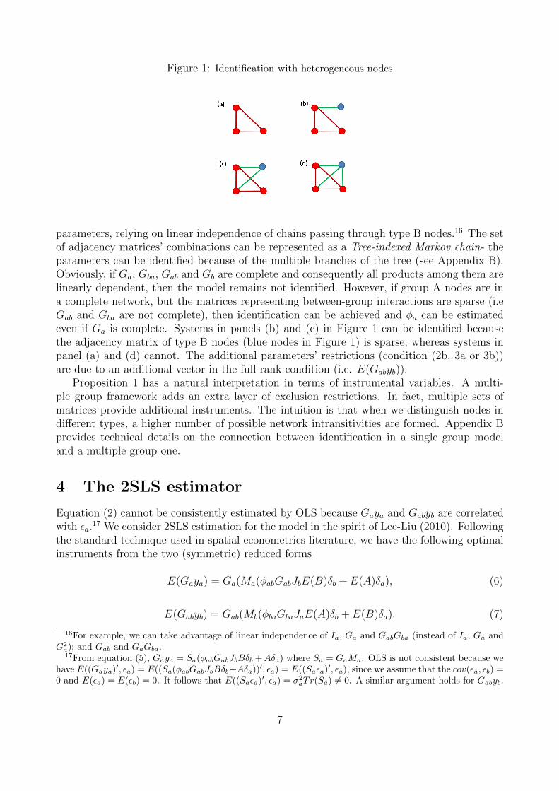
Figure 1: Identification with heterogeneous nodes

parameters, relying on linear independence of chains passing through type B nodes.16 The setof adjacency matrices’ combinations can be represented as a Tree-indexed Markov chain- theparameters can be identified because of the multiple branches of the tree (see Appendix B).Obviously, if Ga, Gba, Gab and Gb are complete and consequently all products among them arelinearly dependent, then the model remains not identified. However, if group A nodes are ina complete network, but the matrices representing between-group interactions are sparse (i.eGab and Gba are not complete), then identification can be achieved and φa can be estimatedeven if Ga is complete. Systems in panels (b) and (c) in Figure 1 can be identified becausethe adjacency matrix of type B nodes (blue nodes in Figure 1) is sparse, whereas systems inpanel (a) and (d) cannot. The additional parameters’ restrictions (condition (2b, 3a or 3b))are due to an additional vector in the full rank condition (i.e. E(Gabyb)).

Proposition 1 has a natural interpretation in terms of instrumental variables. A multi-ple group framework adds an extra layer of exclusion restrictions. In fact, multiple sets ofmatrices provide additional instruments. The intuition is that when we distinguish nodes indifferent types, a higher number of possible network intransitivities are formed. Appendix Bprovides technical details on the connection between identification in a single group modeland a multiple group one.

4 The 2SLS estimator

Equation (2) cannot be consistently estimated by OLS because Gaya and Gabyb are correlatedwith εa.

17 We consider 2SLS estimation for the model in the spirit of Lee-Liu (2010). Followingthe standard technique used in spatial econometrics literature, we have the following optimalinstruments from the two (symmetric) reduced forms

E(Gaya) = Ga(Ma(φabGabJbE(B)δb + E(A)δa), (6)

E(Gabyb) = Gab(Mb(φbaGbaJaE(A)δb + E(B)δa). (7)

16For example, we can take advantage of linear independence of Ia, Ga and GabGba (instead of Ia, Ga andG2

a); and Gab and GaGba.17From equation (5), Gaya = Sa(φabGabJbBδb +Aδa) where Sa = GaMa. OLS is not consistent because we

have E((Gaya)′, εa) = E((Sa(φabGabJbBδb+Aδa))′, εa) = E((Saεa)′, εa), since we assume that the cov(εa, εb) =0 and E(εa) = E(εb) = 0. It follows that E((Saεa)′, εa) = σ2

aTr(Sa) 6= 0. A similar argument holds for Gabyb.

7

Recalling that Za = [Gaya, Gabyb, E(A)] is a n × (k + 2) matrix, we have fa = E(Za) =[E(Gaya), E(Gabyb), E(A)], so from equations (6) - (7) we have

Za = fa + va = fa + [(φabSaGabJbεb + Saεa), (φbaSabGbaJaεa + Sabεb)][e1, e2]′,

where e1 is a first unit vector of dimension (k + 2), Sa = GaMa and Sab = GabMb. Theseinstruments are infeasible given the embedded unknown parameters. fa can be considereda linear combination of IVs in H∗∞ = (Sa(GabJbE(B), E(A)), Sab(GbaJaE(A), E(B)), E(A)).Furthermore, since Sa = GaMa and Sab = GabMb provided ‖φaGa‖∞ + ‖φabφbaCa‖|∞ ≤ 1 and

‖φbGb‖∞ < 1, we have Sa = Ga

∞∑j=0

(φaGa+φabφbaCa)j = Ga

∞∑j=0

(φaGa+φabφbaGab

∞∑j=0

(φjbGjb)Gba)

j.

The same approximation holds for Sab. It follows that

Ca = GabJbGba = Gab(∞∑j=0

φjbGjb)Gba = Gab(

p∑j=0

φjbGjb + (φbGb)

p+1Jb)Gba.

This implies ‖Ca −p∑j=0

φjbGjb‖∞ ≤ ‖(φbGb)

p+1‖∞‖Ca‖∞ = o(1) as p→∞.

Sa = GaMa = Ga

∞∑j=0

(φaGa+φabφbaCa)j = Ga[

p∑j=0

(φaGa+φabφbaCa)j+(φaGa+φabφbaCa)

p+1Sa]→

‖Sa−p∑j=0

(φaGa + φabφbaCa)j‖∞ ≤ ‖(φaGa + φabφbao(1))p+1‖∞‖Sa‖∞ = o(1) as p→∞. Hence,

the approximation error by series expansion diminishes very quickly in a geometric rate, aslong as the degree of approximation (p) increases as n increases. We can also replace Sa andSab by a linear combination. The instruments become

Ha∞ = (Ga(I,Ga, G

2a, . . . (Gab(I,Gb, G

2b , . . . )Gba)) . . . (Gab(I,Gb, G

2b , . . . )E(B), E(A)),

Hab∞ = (Gab(I,Gb, G

2b , . . . (Gba(I,Ga, G

2a, . . . )Gab)) . . . (Gba(I,Ga, G

2a, . . . )E(A), E(B)),

with an approximation error diminishing very quickly when K (or p) goes to infinity, where Kdenotes the number of instruments. Let us define H∞ = [Ha

∞, Hab∞ , X

∗a , GabXb] as the matrix

of instruments and select an na × K submatrix HK based on a p-order approximation ofH∞.18 For instance, if we use the second order approximation of the infinite sums, HK =(Ha

2 , Hab2 , X

∗a , GabXb) will be the first step best projector. The feasible 2SLS estimator for

model (2) isµ = (Z ′aPKZa)

−1Z ′aPKYa, (8)

where µ = (φa, φab, β∗a, γab) and PK = HK(H ′KHK)−1H ′K .

4.1 Asymptotic Properties

This section derives the asymptotic properties of the many-instrument 2SLS estimator forheterogeneous network models. Cohen-Cole et al. (2012) and Liu (2013b) consider a networkmodel with two endogenous variables and one adjacency matrix with multiple networks.19 Our

18Note that K is a function of the degree of approximations p.19Kelejian and Prucha (2004) considers SAR models with multiple endogenous variables and a unique weights

matrix.

8

network model requires two endogenous variables, and two different adjacency matrices.20 InLee and Liu (2010) and Liu (2013b), the asymptotic approximation of the 2SLS estimator isbased on many-instrument asymptotics, where the many instruments derive from the multiplenetwork framework. In our model the many instruments derive from the (approximationof the) multiple adjacency-matrix framework. A multiple matrix framework results in anincreasing number of instruments due to multiple approximations of the optimal instruments.21

This complicates the derivations of the asymptotic properties of the many-instrument 2SLSestimator.

The following propositions establish the consistency and asymptotic normality of the many-instrument 2SLS estimator in equation (8). Regularity conditions together with some discus-sion can be found in Appendix A. Some useful Lemmas are provided in Appendix B. All theproofs are listed in Appendix C. Let

Fa = limn→∞

1

nf ′afa,

22

PKSa = Ψa and PKTba = Ξba, where Tab = SabGbaJb.23

Proposition 2. Under assumptions 1-5, if K/n→ 0, then√n(µ− µ0 − b)

N(0, σ2aF−1a ), where b = (Z ′aPKZa)

−1[e1, e2]σ2a[tr(Ψa), φbatr(Ξba)]

′ = Op(K/n).

From Proposition 2, when the number of instruments K grows at a slower rate thanthe sample size n, the 2SLS estimator is consistent and asymptotically normal. However, theasymptotic distribution of the 2SLS estimator may not be centered around the true parametervalue due to the presence of many-instrument bias of order Op(K/n) (see, e.g., Lee and Liu,2010). We note that the leading order of the bias is the same as in Lee and Liu (2010)and Liu (2013b). However, the structure of the bias differs. Here, it depends on multipleapproximations of the optimal instruments (see the beginning of Section 4). The conditionthat K/n → 0 is crucial for the 2SLS estimator to be consistent. This appears evident ifwe look at the normal equation of our estimator: 1

nZ ′aPK(Ya − Zaµ). When µ = µ0 we have

that E( 1nZ ′aPK(Ya − Zaµ0)) = [e1, e1]σ2

a[tr(Ψa), φbatr(Ξba)]′ = Op(K/n) by Lemma B.2 in the

Appendix. This converges to 0 only if the number of instruments grows more slowly than thesample size.24 N(0,σ2

a(limn→∞1nf ′aP fa)

−1. Note that (Fa − limn→∞1nf ′aP fa) = limn→∞ f

′a(I −

P )fa, which is positive semi-definite in general. The 2SLS estimator with fixed number ofinstrument is generally not efficient. In order to have efficiency, we need to index our matrixof instruments withK and letK grow more slowly than the sample size. The following corollarycharacterizes different scenarios for different rates in which K diverges from n.

Corollary 1. Under assumptions 1-5, (i) if K2/n→ 0,√n(µ− µ0)

N(0, σ2aF−1a ); (ii) if K2/n→ c <∞,

√n(µ− µ0)

N(, σ2aF−1a ), where b = lim

n→∞

√nb.

20We consider the analysis with one network only. The extension to multiple networks extremely complicatesthe notation burden, but the theoretical results remain basically unchanged.

21See Section 4.22This is a crucial assumption. See the discussion in Appendix A after Assumption 4.23To simplify the notation, we assume that n→∞ implies na →∞ and nb →∞.24Indeed, if we use a fixed number of instruments given by H, the asymptotic distribution will be

√n(µ−µ0)

9

The many-instrument bias of the 2SLS estimator can be corrected by the estimated leading-order bias (b) given in Proposition 2. Given consistent estimates of φa, φb, φab, φba, σa and σb,the bias-corrected 2SLS estimator is

µc = (Z ′aPKZa)−1[Z ′aPKYa − σ2

a[e1, e2][tr(Ψa), φba(Ξba)]′]. (9)

The following proposition shows that the bias-corrected estimator is properly centered aroundthe normal distribution.

Proposition 3. Under assumptions 1-5, if K/n → 0 and φa, φb, φab, φba, σa and σb are√n−consistent initial estimators, then

√n(µc − µ0)

N(0,σ2aF−1a ) .

In the next subsection we discuss the case in which the number of endogenous variables(groups) grows with the sample size.

4.2 Estimation with Many Groups

So far, we have assumed that group numerosity does not depend on the sample size. Webelieve that, in practice, such an assumption is virtually always satisfied. For instance, if weincrease the size of the sample, we will always have two genders: male and female. However,for completeness it is interesting to explore whether having the number of groups growingtogether with the sample size affects the estimator properties.

In the many-instrument literature, Anatolyev (2013) and Imbens, Kolesar, et al. (2011)have relaxed the assumption of a fixed number of exogenous regressors. To the best of ourknowledge, the implications of relaxing the assumption of a fixed number of endogenous re-gressors have not been investigated yet.

Let us define g as the number of endogeneous variables and p as the degree of approximation(see Appendix C for an intuition of p as length of chains).

The following proposition characterizes the rate of divergence of g from n.

Proposition 4. if K/n→ 0, we have that g = o(n1/p).

This means, that for our estimator to be consistent and asymptotically normal in thisframework with many instruments and many endogenous variables we need g to grow moreslowly than n1/p.

For completeness, let us consider the link between the number of groups (i.e. endogenousvariables) and the many-instrument asymptotics.

In our framework we have that g/K → 0. In order to have a good performance of theestimator we need K/n → 0. This implies g/n = 1/sg → 0, where sg is the average sizeof groups. In words, in order to have a good performance of the estimators, we need thesize of groups to be large enough. Furthermore, in order to have the estimator properlycentered, we need K2/n → 0. This implies g2/n = g/sg → 0. Therefore, for asymptoticefficiency, the average size of groups needs to be large enough compared to the number ofgroups. These results are similar to those in Lee and Liu (2010). However, the frameworkin Lee and Liu (2010) considers multiple networks embedded in a block-diagonal adjacencymatrix (i.e. G = diag(Ga, Gb)) with the restriction that the within peer effects are the samefor each network, (i.e. φa = φb) and there are no interactions between networks . If a network

10

is defined as a group, then our framework can be considered as a generalization. We havedifferent groups, with both within and between-group interactions. Our adjacency matrix isthus not block-diagonal.

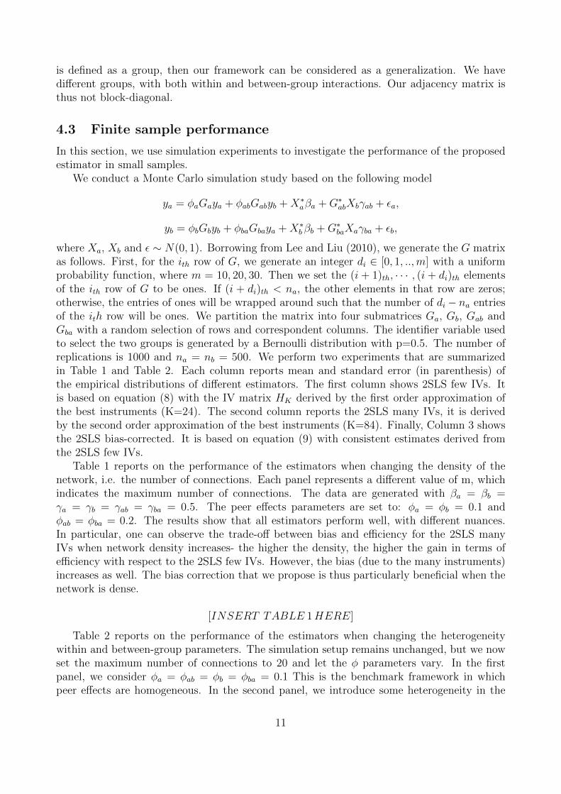
4.3 Finite sample performance

In this section, we use simulation experiments to investigate the performance of the proposedestimator in small samples.

We conduct a Monte Carlo simulation study based on the following model

ya = φaGaya + φabGabyb +X∗aβa +G∗abXbγab + εa,

yb = φbGbyb + φbaGbaya +X∗b βb +G∗baXaγba + εb,

where Xa, Xb and ε ∼ N(0, 1). Borrowing from Lee and Liu (2010), we generate the G matrixas follows. First, for the ith row of G, we generate an integer di ∈ [0, 1, ..,m] with a uniformprobability function, where m = 10, 20, 30. Then we set the (i + 1)th, · · · , (i + di)th elementsof the ith row of G to be ones. If (i + di)th < na, the other elements in that row are zeros;otherwise, the entries of ones will be wrapped around such that the number of di − na entriesof the ith row will be ones. We partition the matrix into four submatrices Ga, Gb, Gab andGba with a random selection of rows and correspondent columns. The identifier variable usedto select the two groups is generated by a Bernoulli distribution with p=0.5. The number ofreplications is 1000 and na = nb = 500. We perform two experiments that are summarizedin Table 1 and Table 2. Each column reports mean and standard error (in parenthesis) ofthe empirical distributions of different estimators. The first column shows 2SLS few IVs. Itis based on equation (8) with the IV matrix HK derived by the first order approximation ofthe best instruments (K=24). The second column reports the 2SLS many IVs, it is derivedby the second order approximation of the best instruments (K=84). Finally, Column 3 showsthe 2SLS bias-corrected. It is based on equation (9) with consistent estimates derived fromthe 2SLS few IVs.

Table 1 reports on the performance of the estimators when changing the density of thenetwork, i.e. the number of connections. Each panel represents a different value of m, whichindicates the maximum number of connections. The data are generated with βa = βb =γa = γb = γab = γba = 0.5. The peer effects parameters are set to: φa = φb = 0.1 andφab = φba = 0.2. The results show that all estimators perform well, with different nuances.In particular, one can observe the trade-off between bias and efficiency for the 2SLS manyIVs when network density increases- the higher the density, the higher the gain in terms ofefficiency with respect to the 2SLS few IVs. However, the bias (due to the many instruments)increases as well. The bias correction that we propose is thus particularly beneficial when thenetwork is dense.

[INSERT TABLE 1HERE]

Table 2 reports on the performance of the estimators when changing the heterogeneitywithin and between-group parameters. The simulation setup remains unchanged, but we nowset the maximum number of connections to 20 and let the φ parameters vary. In the firstpanel, we consider φa = φab = φb = φba = 0.1 This is the benchmark framework in whichpeer effects are homogeneous. In the second panel, we introduce some heterogeneity in the

11

within-group interaction effects. We set φa = φb = 0.1 and φab = φba = 0.3. In the third panel,peer effects are different both within and between groups. We set φa = 0.1, φb = 0.2 φab = 0.4and φba = 0.05. Table 2 shows that the performance of the estimators does not depend on thevalues of the parameters- the ranking of the estimators in terms of efficiency and bias remainsunchanged.


To test the robustness of our results, we have also performed two additional exercises.25

First, instead of using randomly generated networks, we have used the Add Health’s socioma-trix26 as an adjacency matrix, thus replicating features of real-world social networks. Ouraim is to understand whether the results of Table 1 are driven by the random generation oflinks. Second, we use uniform and gamma distributions to generate the errors of the datagenerating process. In doing so, our aim is to investigate whether and to what extent our i.i.d.assumption for the error terms in the derivation of large sample properties affects the finitesample Monte Carlo results. In both cases, the simulation results are very similar to thosereported here.

5 Model Misspecification Bias

In this section, we investigate the bias occurring when the interaction structure is misspecified.First, we analytically derive the bias that occurs when only within-group peer effects are

considered, i.e. when interactions between groups are at work but ignored by the econometri-cian. We then use a simulation experiment to evaluate this bias in finite samples.

Second, we derive the mapping between the parameters of a model with homogeneouspeer effects and those of a model with heterogeneous peer effects. We then use a simulationexperiment to give an example of parameter mapping when peer effects are believed to behomogeneous but are actually heterogeneous in the data generating process (DGP).

Let us suppose the econometrician estimates the following model

ya = (I − φaGa)−1(Xaβa +G∗aXaγa + ε), (10)

whereas the real DGP is

ya = Ga(Ma(φabGabJbBδb + Aδa), (11)

yb = Gab(Mb(φbaGbaJaAδb +Bδa). (12)

25Results available upon request.26A matrix derived from observed connections among students in the Add Health, a program project directed

by Kathleen Mullan Harris and designed by J. Richard Udry, Peter S. Bearman, and Kathleen Mullan Harris atthe University of North Carolina at Chapel Hill, and funded by grant P01-HD31921 from the Eunice KennedyShriver National Institute of Child Health and Human Development, with cooperative funding from 23 otherfederal agencies and foundations. Special acknowledgment is due to Ronald R. Rindfuss and Barbara Entwislefor assistance in the original design. Information on how to obtain the Add Health data files is availableon the Add Health website (http://www.cpc.unc.edu/addhealth). No direct support was received from grantP01-HD31921 for this analysis.

12

This model misspecification results in an estimator of the endogenous effect φa that is incon-sistent. First, we are omitting the influence of the outcome of type B agents. Second, wedo not consider the indirect connections among type A nodes passing through type B nodes.As a result, Gk

a, with k ≥ 2, is misspecified. Therefore, the commonly used instrument G2a

might not be valid as the exclusion restrictions might be violated. Third, we misspecify thecontextual effects (G∗aXa) by ignoring the characteristics of other-type peers. 27

Analytically, the bias is

E(µa) = µa + E(Z ′aPaZa)−1ZaPa(φabGabyb +G∗abXbγab),

where Za = [Gaya, Xa, G∗aXa] and µa = (φa, βa, γa). The bias is positively correlated with the

direct influence of type B on type A, as captured by the peer effects from B to A and theinfluence of the characteristics of type B on type A.

Table 3 shows the extent of this bias in finite samples through a Monte Carlo simulation.Table 3 represents the performance of the 2SLS few IVs following the same experiment designas in the previous section.28 We report on the case in which the maximum number of connec-tions is 10 for each node (as in panel 2 of table 1).29 The first column reports the real valueof the parameters. The second column shows the performance of the 2SLS estimator in themisspecified model. When interactions between groups are at work but ignored by the econo-metrician it results in the size of the bias derived above. The third column shows the results ofthe estimator when the econometrician considers the correct DGP (equations (11) and (12)),but does not use the approximation of optimal instruments (in equation (8)). In other words,we consider the case where the traditional network IV approach is applied mechanically, thusG2aXa and GabGbXb are used as instruments respectively for GaYa and GabYb. In short, only

within-group instruments are considered. The resulting 2SLS estimator is consistent but notefficient. The fourth column reports the performance of our 2SLS few IVs (in equation (8)),which considers the Hk matrix derived in Section 4(i.e which also includes between groupinstruments).30 Mean values for each coefficient’s empirical distribution and standard errors(in parenthesis) are reported.

Table 3 shows that the bias is large in the second column, especially for the β coefficients.In the second column the bias is not large, but the problem is efficiency. Our approach (thirdcolumn) reveals no bias and improved efficiency.


In our second exercise, we consider the case in which the econometrician estimates astandard network model (model (1)) when the real DGP is characterized by heterogeneouspeer effects (model (11) - (12)).

Let us define the following n× n matrices

27This issue also arises when full information about node characteristics and network structure is not avail-able. See Chandrasekhar and Lewis, 2011, Liu, Patacchini, and Rainone, 2013 and Liu, 2013a for problemsrelated to the use of sampled network data.

28We use the 2SLS few IVs to ease the comparison of 2SLS estimators with the misspecified set of instruments.Observe that the bias considered here is due to the misspecification of the model rather than to the many-instrument issue.

29The simulation results in the other cases, i.e. when the maximun number of simulations is 20 or 30, arevery similar.

30First order approximation of optimal instruments is considered.

13

G(a) =

[Ga Oab

Oba Ob

], G(ab) =

[Oa Gab

Oba Ob

],

G(ba) =

[Oa Oab

Gba Ob

], G(b) =

[Oa Oab

Oba Gb

],

where Ol is a l × l matrix of zeros and Olk is a l × k matrix of zeros. Let us suppose forsimplicity that β = βa = βb and γ = γa = γab = γba = γb and focus our attention on the peereffects parameters. In this case model (1) can be written as

Y = φGY +Xβ +G∗Xγ + ε (13)

= (φaG(a) + φabG(ab) + φbaG(ba) + φbG(b))Y +Xβ +G∗Xγ + ε.

Hence, the peer effects parameter, φ, is the following non-linear function of heterogeneous peereffects

φ = φaG−1G(a) + φabG

−1G(ab) + φbaG−1G(ba) + φbG

−1G(b).

If φa = φb = φab = φba = φ, then

φaG(a) + φabG(ab) + φbaG(ba) + φbG(b) = φ(G(a) +G(ab) +G(ba) +G(b)) = φG.

Table 4 contains the results of a simulation experiment in which we estimate model (13), fordifferent values of φa, φb, φab and φba. The simulation set-up is as before- the data generatingprocess remains as in equations (11) and (12)). The estimator considered is the 2SLS few IVs.

In the first column, we set all the φ parameters equal to 0.1. In fact, the 2SLS fewIVs consistently estimates φ = φa = φb = φab = φba. In the second column, we add someheterogeneity. We set φab = 0.3 and φba = 0.3, leaving the other parameters unchanged. Thethird column corresponds to the case in which all the φ parameters are different. As expected,as soon as some heterogeneity is introduced, the estimated value of φ is not informative at all.


6 Impact Evaluation and Treatment Effect

Let us now highlight the importance of our analysis for the identification of treatment responsewith spillovers. Let A be the set of eligible recipients and B the set of ineligible recipients ofa treatment (respectively eligibles and ineligibles hereafter). The treatment is administratedusing a randomized controlled experiment. Having in mind policy interventions such as condi-tional cash transfer or microfinance subsidies can be useful. Let Ta be the binary treatmentvector whose ith element is Ta,i = {0, 1}, which indicates whether i is treated or not (amongthe eligibles).31 Model (2) and (3) can be written as

Ya = φaGaYa + φabGabYb +X∗aβ∗a + δaTa + ρaGaTa +G∗abXbγab + εa, (14)

31Our analysis can be easily adapted to the case of continuous or multinomial treatment. It is also usefulto recall an assumption already listed in the previous sections for estimator properties, G ⊥ Ta, which herestates that the treatment does not change the network topology. This assumption relates to Manski (2013)which assumes that reference groups are person-specific and treatment-invariant (unable to be manipulatedby the policy maker).

14

Yb = φbGbYb + φbaGbaYa +X∗b β∗b +G∗baXaγba +GbaTaρba + εb. (15)

In this model, the Stable Unit Treatment Value Assumption (SUTVA)32 doesn’t hold because(i) spillovers are at work and (ii) spillovers are heterogeneous. To the best of our knowledge,there are no studies that consider violations of the SUTVA because of (ii). This is surprisinggiven that heterogeneity in spillovers is naturally implied by differences between eligibles andineligibles.

Our results in Sections 4 provide consistent and efficient estimators for the parameters ofmodel (2) - (3).33

6.1 Average Treatment Effect with Heterogeneous Spillovers

The Average Treatment Effect in our context can be written as34

ATE = E(Yi|i ∈ A, Ta,i = 1, X,G)− E(Yi|i ∈ A, Ta,i = 0, X,G). (16)

From the reduced form of equation (14)

ATE = δaEET (ma,ii), (17)

where ma,ii is the iith element of Ma and EET (·) = E(·|i ∈ A, Ta,i = 1, X,G) indicates theexpected value over the treated eligibles. The Average Treatment Effect is thus equal to thedirect impact of the treatment on the individual i (i.e. δa) plus the indirect effect of otheragents’ spillovers on i triggered by i’s treatment (but not triggered by other nodes’ treatment)

δaMa = δaIa + δa

∞∑k=1

(φaGa + φabφbaCa)k.

Observe that ma,ii is a function of (Ga, Gb, Gab, Gba, φa, φb, φab, φba). This implies that whennetwork interactions are at work, the ATE depends on network topology and strength ofoutcome spillovers among agents. As a result, an individual can have a high increase inoutcome even if she has a low treatment direct impact (a low δa) but she is central in thenetwork.35 Observe that even if δa,i = δa( i.e. the treatment effect is homogenous) the ATEcan be heterogeneous because of the different position of nodes in the network. Indeed, theATE can be decomposed into two parts

ATE = δa︸︷︷︸DTE

+ δaEET [(diag(Ma − Ia)]︸︷︷︸FLTE

. (18)

32Following Rubin (1986), SUTVA states that potential outcomes depend on the treatment received, andnot on what treatments other units receive and that there are no ”hidden treatments”.

33As mentioned in the Introduction, we do not consider direct treatment effect heterogeneity. This assump-tion can be relaxed, allowing for a double form of heterogeneity: one coming from individual characteristics,the other from the interactions. The identification becomes much more complex. We leave this extension forfuture research. Following Manski (2013), we also assume here that the treatment does not change the networktopology, i.e. that the policy maker cannot manipulate reference groups.

34When the treatment is a randomized control experiment, the average treatment effect is equal to theaverage treatment effect on treated.

35Of course the centrality itself is not a sufficient condition, a high level of spillovers is required.

15

The first part is the Direct Treatment Effect (hereafter DTE), whereas the second part is theeffect of the treatment due to the interactions among agents, i.e. the effect of i’s treatmentthat impact i through other nodes. We denote the latter effect as Feedback Loop TreatmentEffect (hereafter FLTE). The sample counterpart of equation (18) is

ˆATE = µ′t[δadiag(Ma)]µt1

nta= δa

1

nta

∑i∈NT

a

ˆma,ii, (19)

where NTa is the set of treated individuals which has cardinality nta < na, µt is the nta × 1

selector vector for that units and Ma = Ma(φa, φb, φab, φba) is the estimated counterpart ofMa.

Treatment Effect Misinterpretation and Bias When SUTVA holds, ATE = DTE.If interferences are at work, then ATE 6= DTE. However, the problem is not only aboutinterpretation. We show below that if spillovers are ignored, then the parameter estimatescan be inconsistent. Suppose that a treatment is administered to nta < na subjects and weignore interactions among them. Estimation of δa is based on the following regression

Ya = Xaβa + Taδa + ε∗a, (20)

where ε∗a = ρaGaTa +φaGaYa +φabGabYb + εa contains the three relevant spillover effects omit-ted:36 (i) the direct treatment spillover from other eligibles ρaGaTa, (ii)the endogenous out-come spillover from other treated eligibles φaGaYa and (iii) the endogenous outcome spilloverfrom ineligibles φabGabYb. Misinterpretation occurs because the estimate of δa is interpretedas a DTE while, if the data generating process is given by equations (14) and (15), it is anATE. Bias can occur if the treatment is correlated with the three components listed above

δa = δa + bias = δa + (T ′aTa)−1Ta { ρaGaTa

+ φaGaMa[φabGabJb(ρbaGbaTa) + Taδa + ρaGaTa]

+ φabGabMb[φbaGbaJa(δaTa + ρaGaTa) + ρbaGbaTa]}.

The bias is due to the spillover effects coming from the three omitted components listedbefore. By correctly specifying the interaction structure we can consistently estimate thedirect treatment effect purged of the influence of the three omitted components.

It should appear clear from our discussion that, if the spillovers’ coefficients and the directtreatment effect are positive, neglecting between and within-group interactions result in anoverestimation of the direct treatment effect. Manski (2013) defines this scenario as Rein-forcing Interactions. Of course one can imagine different scenarios where interactions are notreinforcing and, on the contrary, are Opposing Interactions.

Our approach has an advantage from this point of view- it allows interactions betweenand within groups to be heterogeneous (e.g. Reinforcing Interactions within groups membersand Opposing Interactions between groups). We also note that, using again Manski (2013)’sterminology, our framework can be adapted to the estimation of social interaction with leadersand followers, labeling those agents as groups A and B.

36The other omitted terms, X∗aβ∗a and G∗abXbγab, are independent from the treatment.

16

6.2 Indirect Treatment Effect

As mentioned before, the Indirect Treatment Effect (hereafter ITE) has been an object ofinterest in several papers. Most of the existing papers focus attention on the indirect effecton ineligibles (see, e.g. Angelucci and De Giorgi, 2009). However, when the population issplit into two sets, it is also natural and interesting from a policy perspective to understandwhether different types of untreated (eligible or ineligible), are differently impacted by thetreatment. Let us define ITEE and ITEI as the Indirect Treatment Effect on Eligibles andthe Indirect Treatment Effect on Ineligibles, respectively.

The Indirect Treatment Effect on Eligibles in our model is

ITEE = E(Yi|i ∈ A,MiT 6= 0∩Ta,i = 0, X,G)−E(Yi|i ∈ A,MiT = 0∩Ta,i = 0, X,G), (21)

whereas the Indirect Treatment Effect on Ineligibles can be defined as

ITEI = E(Yi|i ∈ B,MiT 6= 0, X,G)− E(Yi|i ∈ B,MiT = 0, X,G), (22)

where Mi is the ith row of M =

([IaIb

]−[Gaφa GabφabGbaφba Gbφb

])−1

, T = [Ta, 0b], and 0b is a

nb×1 vector of zeros. MiT = 0 indicates that i is not affected by any of the treated nodes (i.e.that there are no direct and indirect paths in the networks between i and a treated node).

Let us now suppose that, given our data generating process (equations (14) and (15))we are asked by a policy maker to evaluate the Indirect Treatment Effects after a treatmentadministered to the eligibles (i.e. to a subset of A). From model (14) - (15) we can derive thefollowing formulas

ITEE = EEu [Mai(φabGabJb(ρbaGbaTa) + δaTa + ρaGaTa)],

ITEI = EI [Mbi(φbaGbaJa(δaTa + ρaGaTa) + ρbaGbaTa)],

where Mai is the ith row of Ma, Mbi is the ith row of Mb , EI(·) = EI(·|i ∈ B,MiT 6= 0, X,G)indicates the expected value over the (indirectly treated) ineligibles, and EEu(·) = E(·|i ∈A,MiT 6= 0 ∩ Ta,i = 0, X,G) indicates the expected value over (indirectly treated) untreatedeligibles. Observe that these estimands depend on direct and indirect connections becauseof network-based spillovers. More formally, they can be decomposed into different parts.For instance, ITEE may be decomposed into three effects. The first term , δaMa, capturespropagation of the treatment via outcome spillovers.37.

The nice feature of this derivation of ITEI and ITEE is that instead of simply addressingthe question whether an ITE is different from zero, we can also decompose it into differentsources of treatment’s transmission. For instance, one can find that the treated population

37Given that Ma = (I−φaG−φabφbaCa)−1, we have Maδa = Iaδa+[(Ia−φaG−φabφbaCa)−1−I]δa. The firstterm is the diagonal matrix of treatment direct effects which has (by definition) no impact on the untreated,while the second term represents the propagation of those effects through the network via endogenous spillovers(i.e. changes in outcomes due to treatment). The second term, ρaMaGa, measures the spillover arising fromthe treatment given to other units (ρaGa), as well as its amplification through interactions (as captured byMa). Finally, φabρbaMaGabJbGba, denotes the spillover accruing to ineligibles distinguished between outcomeamplification (MaGabJb) and (indirect) treatment effect (ρbaGba). A similar decomposition can be applied toITEI

17

has a strong reaction to the treatment (δa and ρa are high) and transmits it to ineligiblesthrough low magnitude peer effects (φab is low). The same level of ITEI, however, can alsoarise from a scenario where there is a low reaction to the treatment within group (δa and ρaare low) and a large transmission between groups (φab is high).

Understanding these different channels is paramount for policy purposes. Most impor-tantly, our framework enables the researcher to distinguish the role of contextual effects frompeer effects in transmitting the treatment. In other words, one can quantify how much ofthe effect is generated by the direct effect of the treatment through exogenous variables (ascaptured by δa, ρa and ρba) and how much is due to spillovers through outcomes (as capturedby φba, φa, φb and φab). Note also that having these estimates at hand, one can understandwhich effects (within eligibles, within ineligibles and between them) are the dominant ones inspreading out the policy’s beneficial effect.

We can thus simply use the sample counterpart to estimate the ITEE and ITEI

ÎTEE = µ′u[Ma(φabGabJb(Gbaγba) + βa +Gaγa)]µu1

nua,

ÎTEI = ι′b[Mb(φbaGbaJa(βa +Gaγa) +Gbaγba)]ιa1

nb,

where nua < na is the number of eligibles who are untreated, µu is the na × 1 selector vectorfor that units and ιl is an nl × 1 vector of ones.

6.3 Total Treatment Effect

One can also be interested in evaluating the treatment effect on the entire population (ornetwork). As the SUTVA has been removed and spillovers are in place, it is useful to derivethe Total Treatment effect (hereafter TTE). Following our previous notation we have thefollowing definition for TTE

TTE = E(Yi|i ∈ A ∪B,MiT 6= 0, X,G)− E(Yi|i ∈ A ∪B,MiT = 0, X,G).

This represents the treatment effect on a generic individual in the network (eligible or ineligi-ble). Its sample counterpart is

ˆTTE = ι′([

IaIb

]−[Gaφa GabφabGbaφba Gbφb

])−1(δa

[TaOb

]+

[Gaρa Gab

Gbaρba Gb

] [TaOb

])ι1

n,

where ι is an n × 1 vector of ones. Note that the ˆTTE is basically the weighted average ofÂTE, ÎTEE, and ÎTEI.

6.4 Control Group

It is well-known that the ATE, ITEE, ITEI and TTE are identified if we have a controlgroup, i.e. if we can distinguish sample of units who are not treated (directly or indirectly).This can be quite challenging when estimating the indirect treatment effects. In a networkcontext, we have two possibilities: (i) a multiple network-based approach and (ii) topology-driven approach.

18

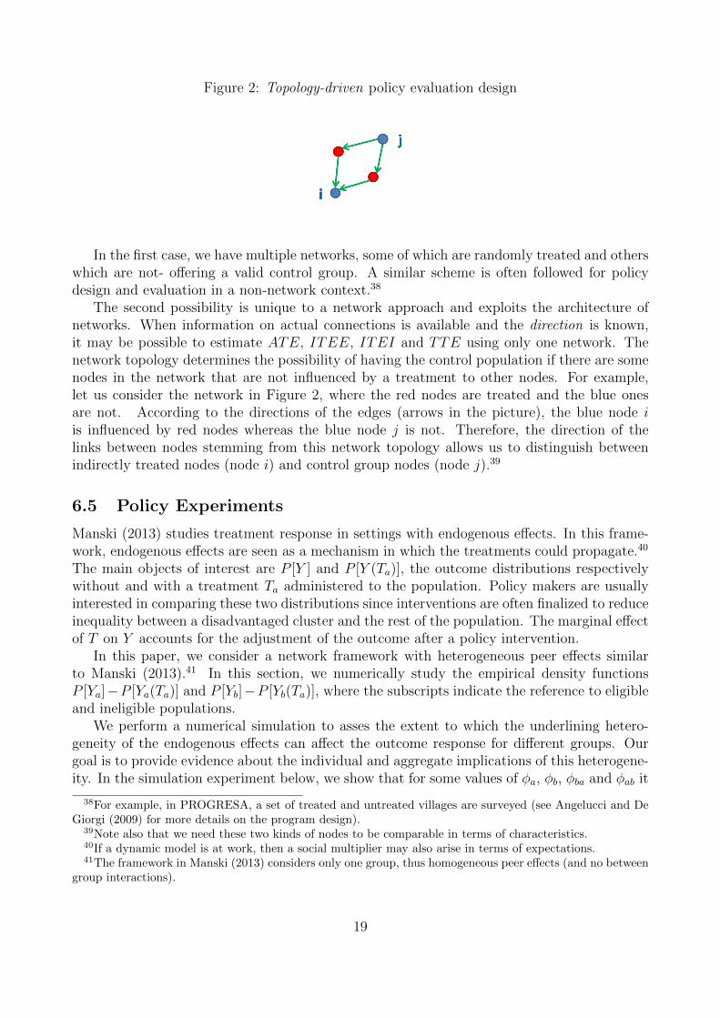
Figure 2: Topology-driven policy evaluation design

In the first case, we have multiple networks, some of which are randomly treated and otherswhich are not- offering a valid control group. A similar scheme is often followed for policydesign and evaluation in a non-network context.38

The second possibility is unique to a network approach and exploits the architecture ofnetworks. When information on actual connections is available and the direction is known,it may be possible to estimate ATE, ITEE, ITEI and TTE using only one network. Thenetwork topology determines the possibility of having the control population if there are somenodes in the network that are not influenced by a treatment to other nodes. For example,let us consider the network in Figure 2, where the red nodes are treated and the blue onesare not. According to the directions of the edges (arrows in the picture), the blue node iis influenced by red nodes whereas the blue node j is not. Therefore, the direction of thelinks between nodes stemming from this network topology allows us to distinguish betweenindirectly treated nodes (node i) and control group nodes (node j).39

6.5 Policy Experiments

Manski (2013) studies treatment response in settings with endogenous effects. In this frame-work, endogenous effects are seen as a mechanism in which the treatments could propagate.40

The main objects of interest are P [Y ] and P [Y (Ta)], the outcome distributions respectivelywithout and with a treatment Ta administered to the population. Policy makers are usuallyinterested in comparing these two distributions since interventions are often finalized to reduceinequality between a disadvantaged cluster and the rest of the population. The marginal effectof T on Y accounts for the adjustment of the outcome after a policy intervention.

In this paper, we consider a network framework with heterogeneous peer effects similarto Manski (2013).41 In this section, we numerically study the empirical density functionsP [Ya]−P [Ya(Ta)] and P [Yb]−P [Yb(Ta)], where the subscripts indicate the reference to eligibleand ineligible populations.

We perform a numerical simulation to asses the extent to which the underlining hetero-geneity of the endogenous effects can affect the outcome response for different groups. Ourgoal is to provide evidence about the individual and aggregate implications of this heterogene-ity. In the simulation experiment below, we show that for some values of φa, φb, φba and φab it

38For example, in PROGRESA, a set of treated and untreated villages are surveyed (see Angelucci and DeGiorgi (2009) for more details on the program design).

39Note also that we need these two kinds of nodes to be comparable in terms of characteristics.40If a dynamic model is at work, then a social multiplier may also arise in terms of expectations.41The framework in Manski (2013) considers only one group, thus homogeneous peer effects (and no between

group interactions).

19

may be (paradoxically) more convenient to treat a group other than the target one. This hasimplications for the study of socio-economic inequality. Importantly, by allowing estimationof all the different parameters of interest, our model specification can be used to understandwhat nodes (or which type of nodes) should be targeted by a social planner whose final goalis to maximize an aggregate outcome or to converge to a desired distribution of individualoutcomes.

We present an experiment where we treat a random sample of nodes and simulate thetreatment’s propagation through a network characterized by heterogeneous peer effects. Morespecifically, we look at the increase of type A and type B nodes’outcomes once a certain setof nodes receives a treatment42.

Two exercises are implemented. In the first, we evaluate aggregate effects, i.e. the changein the sum of outcomes (for both type A and type B individuals) which follows a treatmentfor different values of peer effects (i.e. φa, φb, φba, φab). In the second exercise, we look atdistributional effects, i.e. at changes in the empirical distribution of individual node outcomesfor different sets of peer effects parameters following the policy intervention .

Figures 5 and 6 report on the first exercise. Figure 5 depicts the results when fixing φb =φba = 0.1 and varying φa and φab. We generate a grid of values for parameters resulting fromtwo sequences: φa = 0.02, 0.04, ..., 0.50 and φab = 0.02, 0.04, ..., 0.50. For each couple (φa, φab)we generate one hundred independent replications using the same DGP as described in Section4.3 and compute Y s

a =∑

i∈A yi and Y sb =

∑i∈B yi. We then select a random sample of one

hundred type A nodes to be treated. This treatment is represented by an na × 1 vector Ta ofzeros for non treated nodes and ones for treated nodes. Finally, we compute Y s∗

a =∑

i∈A y∗i

and Y s∗b =

∑i∈B y

∗i , where y∗i = yi + ∂yi

∂TaTA. This exercise represents the case where group A

nodes are treated and there are low interactions between nodes A and nodes B (φba = 0.1).From equations (14) and (15) we have

∆yi = y∗i − yi =∂yi∂Ta

Ta ={

Mai (φabGabJb(ρbaGbaTa) + (δa +Gaρa)Ta) if i ∈ AMbi (φbaGbaJa(δa + ρaGa)Ta + ρbaGbaTa) if i ∈ B .

Figure 5 represents the differences ∆Y sa = Y s∗

a − Y sa =

∑∂Ya∂Ta

Ta and ∆Y sb = Y s∗

b − Y sb =∑ ∂Yb

∂TaTa for all the possible combinations (φa, φab).

43

Figure 5 shows that ∆Y sa increases steadily with φa (and slightly with φab), whereas ∆Y s

b

remains roughly unchanged. These results are not surprising. If there are no interactions (orlow interactions) between the two groups, then there is no reason why the outcome of group

42We compute the marginal effect matrix of Ta on Ya multiplied by the treatment vector

∂E(Ya|G,X)

∂TaTa = Ma(φabGabJb(ρbaGbaTa) + δaTa + ρaGaTa).

Note that when there are no interactions between the two groups (or only type A nodes are considered in the

analysis), we have ∂E(Ya|G,X)∂Ta

Ta = Sa(δaTa + ρaGaTa), where Sa = (I − φa)−1. This is the marginal effectmatrix in a standard peer effects model.

The marginal effect matrix of Ta on Yb is

∂E(Yb|G,X)

∂TaTa = Mb(φbaGbaJa(δaTa + ρaGaTa) + ρbaGbaTa). (23)

Observe that the marginal effect of Ta on Ya is different from the marginal effect of Ta on Yb -an increase inTa differently affects nodes depending on their type.

43Some combinations are missing in the grid because it is unlikely to draw Ga and Gab such that ‖φaGa‖∞+‖φabφbaCa‖|∞ ≤ 1. These combinations are at the edge of the parameter space.

20

B should change. The variation in the outcome of the group A depends on the extent of theendogenous effects (φa). If instead there are interactions between the two groups, then thetreatment response depends on both φa and φab. For example, assuming a positive effect ofthe independent variable, if a policy intervention targets a group when the two groups havethe same outcome profile, we expect an increase in inequality in terms of outcomes betweenthe two types when the within-peer effects (φa) are high and the between-peer effects (φab)are low.

[INSERT FIGURE 5HERE]

Figure 6 depicts the results when fixing φb = φab = 0.1, and varying φa and φba. Theexperiment design remains unchanged. This exercise represents the case where group A nodesare treated and there are increasing influences within nodes A and from nodes A and nodes B(φba increasing up to 0.5). Figure 6 shows that an increase of φba is beneficial for ∆Y s

b , as type Bnodes receive an impulse from type A nodes. Interestingly, type B nodes may actually benefiteven more than A nodes (the treated group). Our results shows that when φba > 0.20, weobserve ∆Y s

b > ∆Y sa . In terms of policy effects, this means that if a policy targets one group

but peer effects between groups are high, then we can observe increasing inequality betweenthe two groups, rather than the expected decrease (assuming that the targeted group has alower starting outcome). In terms of the estimands derived in Section 6 , note that the bluesurfaces in Figures 5 and 6 are simply ITEI×nb while the red ones are ITEE×nua+ATE×nta,plotted for different combinations of parameters.


In the second exercise, we consider four points from the grid formed by φa and φba andlook at the empirical distributions of ∆yi∈A and ∆yi∈B . We estimate these distributions usinga normal kernel density. We consider the case where φa = 0.1 and φba = 0.1 as a benchmarkand then increase the strength of peer effects among agents in different ways.

In Figure 7 we increase the effect within group A only (φa = 0.3.). While this change isirrelevant for type B nodes, it has interesting implications for the distribution of outcomesamong type A nodes (Panel a). While in the benchmark model (the single line), the distribu-tion is quasi-bimodal (due to the treated and non-treated A nodes), an increase of φa smoothsthe distribution (the bold line). In other words, the higher the endogenous effects, the moreevenly the benefits of the policy intervention are shared among nodes (individuals).


In Figure 8 we increase the between-group effect only (φba = 0.3). Type A density remainsbasically unchanged (Panel a) . The impact is instead apparent on the outcome distributionof type B nodes (Panel b). One can observe an important shift to the right. This means thatnon treated type B nodes benefit more than non-treated type A nodes ( from the treatmentto type A nodes).

The red and blue curves in Figures 7 and 8 are the empirical density functions P [Ya(Ta)−Ya]and P [Yb(Ta)− Yb], respectively. They have ITEE×nua+ATE×nta

naand ITEI as expected values.


21

7 Concluding Remarks

We generalize the linear-in-means model to the presence of two groups and between-groupinteractions. We derive the sufficient conditions to identify the model and propose efficient2SLS estimators. We characterize the bias which arises when interactions are ignored andevaluate it in finite sample using simulation experiments. We illustrate the relevance of theseissues for policy purposes. If peer effects are seen as a mechanism in which the treatments couldpropagate through the networks, then accounting for heterogeneous peer effects and between-group interactions can be helpful in designing and evaluating policy interventions that alter theoutcome distribution. We show that when between-group interactions are strong, an impulse toa given group can engender benefits to another group which are even higher than those accruingto the target group. Examples of types of interventions where the local non-target populationmay also be indirectly affected by the treatment through social and economic interactionwith the target population are widely varied. For example, the recipients of conditional cashtransfers may share resources with ineligible households who live in the same community orwith extended family members, which could affect the incentives to accumulate human capital(Angelucci et al., 2010). School vouchers or other incentives (such as equipment provision) toincrease schooling of indigent children may increase the learning ability of untreated children if,for example, textbooks or computers are shared among classmates. A number of organizationspromote the deworming of children in the developing world as a public health and developmentstrategy. Supplying deworming drugs to a group of children may benefit untreated childrenby reducing disease transmission, thus lowering infection rates for both groups.

In sum, our paper contributes to the literature by providing a framework able to decomposethe treatment response into different components, including the crucial difference betweenendogenous effects and effects stemming from exogenous variations in the characteristics ofthe treated.

22

References

Anatolyev, Stanislav (2013). “Instrumental variables estimation and inference in the presenceof many exogenous regressors”. In: The Econometrics Journal 16.1, pp. 27–72.

Angelucci, M. et al. (2010). “Family networks and school enrolment: Evidence from a random-ized social experiment”. In: Journal of Public Economics 94.3a4, pp. 197–221.

Baltagi, B. H., C. Kao, and L. Liu (2012). “On the Estimation and Testing of Fixed EffectsPanel Data Models with Weak Instruments”. In: Advances in Econometrics 30, pp. 199–235.

Bekker, P. A. (1994). “Alternative approximations to the distributions of instrumental variableestimators”. In: Econometrica, pp. 657–681.

Benjamini, I. and Y. Peres (1994). “Markov chains indexed by trees”. In: The annals ofprobability 22, pp. 219–243.

Bramoulle, Y., H. Djebbari, and B. Fortin (2009). “Identification of peer effects through socialnetworks”. In: Journal of Econometrics 150, pp. 41–55.

Chandrasekhar, A. and R. Lewis (2011). “Econometrics of sampled networks”. In: Unpublishedmanuscript, MIT.[422].

Chipman, Hugh A, Edward I George, Robert E McCulloch, et al. (2010). “BART: Bayesianadditive regression trees”. In: The Annals of Applied Statistics 4.1, pp. 266–298.

Cohen-Cole, E., X. Liu, and Y. Zenou (2012). “Multivariate Choice and Identification of SocialInteractions”. In: CEPR Discussion Paper No. DP9159.

Crump, Richard K et al. (2008). “Nonparametric tests for treatment effect heterogeneity”. In:The Review of Economics and Statistics 90.3, pp. 389–405.

Donald, S. and W. Newey (2001). “Choosing the Number of Instruments”. In: Econometrica69.5, pp. 1161–1191.

Firpo, Sergio (2007). “Efficient Semiparametric Estimation of Quantile Treatment Effects”.In: Econometrica 75.1, pages.

Goldsmith-Pinkham, P. and G. Imbens (2013). “Social networks and the identification of peereffects”. In: Journal of Business and Economic Statistics 31, pp. 253–264.

Hsieh, C. S. and L. F. Lee (2011). A Social Interactions Model with Endogenous FriendshipFormation and Selectivity. Tech. rep. Working paper.

Hudgens, M. and E. Halloran (2008). “Toward Causal Inference With Interference”. In: Journalof American Statistical Association 103, pp. 832–842.

Imai, Kosuke, Marc Ratkovic, et al. (2013). “Estimating treatment effect heterogeneity inrandomized program evaluation”. In: The Annals of Applied Statistics 7.1, pp. 443–470.

Imbens, G., M. Kolesar, et al. (2011). “Identification and Inference with Many Invalid Instru-ments”. In:

Imbens, G. and G. Woolridge (2009). “Recent Developments in the Econometrics of ProgramEvaluation.” In: Journal of Economic Literature 47(1), pp. 5–86.

Jackson, M.O. and Y. Zenou (forthcoming 2013). Economic Analyses of Social Networks.Kelejian, H. and I. R. Prucha (1998). “A generalized spatial two-stage least squares procedure

for estimating a spatial autoregressive model with autoregressive disturbances”. In: TheJournal of Real Estate Finance and Economics 17.1, pp. 99–121.

— (1999). “A generalized moments estimator for the autoregressive parameter in a spatialmodel”. In: International economic review 40.2, pp. 509–533.

23

Kelejian, H. and I. R. Prucha (2001). “On the asymptotic distribution of the Moran I teststatistic with applications”. In: Journal of Econometrics 104.2, pp. 219–257.

— (2004). “Estimation of simultaneous systems of spatially interrelated cross sectional equa-tions”. In: Journal of Econometrics 118.1, pp. 27–50.

— (2007). “HAC estimation in a spatial framework”. In: Journal of Econometrics 140.1,pp. 131–154.

LeBlanc, Michael and Charles Kooperberg (2010). “Boosting predictions of treatment success”.In: Proceedings of the National Academy of Sciences 107.31, pp. 13559–13560.

Liu, X. (2013a). “Estimation of a local-aggregate network model with sampled networks”. In:Economics Letters 118.1, pp. 243–246.

Liu, X. and L. F. Lee (2010). “GMM estimation of social interaction models with centrality”.In: Journal of Econometrics 159, pp. 99–115.

Liu, X., E. Patacchini, and E. Rainone (2013). “The Allocation of Time in Sleep: A SocialNetwork Model with Sampled Data”. In: CEPR Discussion Paper No. DP9752.

Liu, X., E. Patacchini, and Y. Zenou (2014forthcoming). “Endogenous peer effects: LocalAggregate or Local Average?” In: Journal of Economic Behavior and Organization.

Manski, C. F. (1993). “Identification of endogenous social effects: The reflection problem”. In:The review of economic studies 60.3, pp. 531–542.

— (2013). “Identification of treatment response with social interactions”. In: The Economet-rics Journal 16.1, S1–S23. issn: 1368-423X.

Miguel, Edward and Michael Kremer (2004). “Worms: Identifiying Impacts on Eduaction andHealth in the Presence of Treatment Externalities”. In: Econometrica 72, pp. 159–217.

Rubin, D. (1986). “Which ifs have causal answers? Discussion of Hollands Statistics and causalinference””. In: Journal of the American Statistical Association 81, pp. 961–962.

Sinclair, Betsy, Margaret McConnell, and Donald P. Green (2012). “Detecting Spillover Ef-fects: Design and Analysis of Multilevel Experiments”. In: American Journal of PoliticalScience 56, pp. 1055–1069.

Staiger, D. and J. H. Stock (1997). “Instrumental Variables Regression with Weak Instru-ments”. In: Econometrica 65.3, pp. 557–586.

24

APPENDIX

Appendix A: Assumptions and Discussions

Let us introduce some notation and assume the following regularity conditions: a sequenceof square matrices {A}, where A = [Aij], is defined ”uniformly bounded in absolute value”(UB) if there exists a constant cb < ∞ (that does not depend on n) such that ‖A‖∞ =maxi=1,··· ,n

∑nj=1|Aij| < cb and ‖A‖1 = maxj=1,··· ,n

∑ni=1|Aij| < cb. We indicate that {A} is

bounded only in row (column) sum absolute value as UBR (UBC). For the sake of simplicitywe will assume that n→∞ implies na →∞ and nb →∞.

Assumption 1. The elements of εa and εb are iid with zero mean, variance σ2a and σ2

b respec-tively, and zero covariance. Moments higher than the fourth exist.

Assumption 2. The elements of Xa and Xb are uniformly bounded constants, Xa and Xb

have full rank k, and limna→∞

1naX ′aXa and lim

nb→∞1nbX ′bXb are finite and non singular.

Assumption 3. The sequences of matrices {Ga}, {Gab}, {Gb}, {Gba}, {Ma}, {Mb}, {Jb},and {Ja} are UB.

The first assumption is needed in order to apply the Kelejian and Prucha (2001) CentralLimit Theorem (CLT) of a linear and quadratic form. Assumption 2 is standard in theliterature. Assumption 3 is exploited in Kelejian and Prucha (1999) to limit the spatialdependence among the units. It rules out any spatial unit root case. As Lee (2004) pointedout, it plays an important role in the derivation of asymptotic properties of the estimatorsfor spatial econometric models. It guarantees that the variance of Ya and Yb is bounded asn goes to infinity. Observe that this assumption is also crucial for the identification of theheterogeneous network model, as shown in Proposition 1.

Assumption 4 is a sufficient condition for identification of the social network model. Forassumption 4 to hold, E(Za) must be full column rank for large enough na.

Assumption 4. Fa = limn→∞

1nf ′afa is finite and a full rank matrix, Fb = lim

n→∞1nf ′bfb is finite

and a full rank matrix.

Since the variance of the structural error is var(va) and the concentration parameter (whichmeasures the instrument’s strength) is f ′afa/var(va), this assumption implies that the concen-tration parameter grows at the same rate as the sample size. Such a rate is assumed inBekker (1994). Hence, we assume that the instruments are stronger than assumed in theweak-instrument literature.44 For the sake of brevity we focus on equation (2), and we implythe same argument holds for equation (3).

Assumption 5. There exists a K × (k + 2) matrix ΘK such that 1n‖E(Za)−HKΘK‖2 → 0

as n,K →∞.

44See Staiger and Stock, 1997 or Baltagi et al., 2012 for a panel data version of weak-instrument asymptotics.Another interesting extension could be to derive the estimator’s asymptotic properties under many weakinstruments. In doing so, we are allowing the rate of concentration parameter to be different than the rate ofthe sample size. Consequently, we can compare it with the rate in which K increases. See for example, Chaoand Swanson (2005)

25

Following Lee and Liu(2010), assumption 5 requires that the (infeasible) best IV matrixcan be well approximated by a certain linear combination of the feasible IV matrix HK as thenumber of instruments increases with the sample size. Once we assume this, we can deal withthe approximation of Sa and Sab. We have to approximate this matrix since we cannot use itas matrix of instruments because it is formed by unknown parameters. If HK has the followingstructure then assumption 5 holds and we can obtain efficiency under certain conditions.

Proposition 5. If ‖φaGa‖∞+‖φabφbaCa‖∞ < 1, let us define H(p)K = (H

a(p)K , H

b(p)K , X∗a , GabXb)

where

Ha(p)K = (Ga(Ga, (Gab(Gb, . . . , G

p+1b )Gba), . . . , (Ga(Ga, (Gab(Gb, . . . , G

p+1b )Gba)

p+1(E(A), GabJbB),

Hb(p)K = (Gab(Gb, (Gba(Ga, . . . , G

p+1a )Gab), . . . , (Gb(Gb, (Gba(Ga, . . . , G

p+1a )Gab)

p+1(E(B), GbaJaA),

where p is an increasing integer valued function of K, there exists a K × (k + 2) matrix Θ(p)K

such that ‖fa −H(p)K Θ

(p)K ‖∞ → 0 as n,K →∞.

Therefore, the 2SLS estimator can be asymptotically efficient when we use an increasingnumber of instruments.

26

Appendix B: Some Useful Lemmas

Lemma 1. Recall that Za = fa + va. Let ef = 1nf ′a(I − PK)fa. As K/n = O(1): (i) Tr(ef ) =

o(1) (ii) v′aPKva = Op(K). (iii) f ′aPKva = Op(√nK). (iv) ef = O(tr(ef )). (v) 1

nZ ′aPKZa =

1nf ′afa − ef + 1

nf ′aPKva + 1

nv′aPKfa + 1

nv′aPKva = Op(1).

Proof. (i) See lemma B.3 (i) in Lee and Liu (2010).(ii) Let us write v′aPKva = ε′aS

′aPKSaεa+ε′bJ

′bG′baS′abPKSabGbaJbεb. Let us focus on the first

term of the sum, since E|ε′aS ′aPKSaεa| = E[tr(|ε′aS ′aPKSaεa|)] = σ2atr(|PKSaS ′aPK |) = O(K)

by lemma B.2 (ii) Lee and Liu (2010), then by Markov’s Inequality Pr(|εaS ′aPKSaεa|) ≥ α) ≤E(|εaS′aPKSaεa|)

α= Op(K).

For the second part of the sum, given also that SabGbaJb = Tab where Tab is UB, we canapply the same proof and obtain the same order of probability. We then have O(f(x))+O(f(x))=O(f(x)).

(iii) For each j we have by Cauchy-Schwarz inequality |e′jf ′aPKva| ≤√e′jf′afaej

√εaS ′aPKSaεa =

O(√n)Op(

√K) = Op(

√nK).

(iv) By lemma A.3 (ii) in Donald and Newey (2001).(v) 1

nZ ′aPKZa = 1

nf ′afa −O(tr(ef )) +Op(K/n) +Op(

√K/n) = Op(1).

Lemma 2. Recall that Za = fa + va, let PKSa = Ψa and PKTba = Ξba . As K/n = O(1): (i)E(v′aPKεa) = σ2

a[e1, e2][tr(Ψa), φba(Ξba)]′. (ii)E(v′aPKεaε

′aPKva) = σ4

atr2([(Ψa), (Ξba)]) +O(K).

(iii) [Z ′aPKεa− [σ2a[e1, e2][tr(Ψa), φbatr(Ξba)]

′/√

(n)] = f ′aεa/√n+Op(

√K/n)+Op(

√tr(ef )) =

f ′aεa/√n+Op(1).

Proof. (i) E(v′aPKεa) = [e1, e2]E([(φabSaGabJbεb + Saεa), (φbaSabGbaJaεa + Sabεb)]′)PKεa =

[e1, e2][E(ε′aS′aPKεa), E(φbaε

′aJ′aG′baS′abPKεa)]

′ = σ2a[e1, e2][tr(Ψa), φbatr(Ξba)]

′.(ii) By lemma A.2 in Lee (2001), E(v′aPKεaε

′aPKva) = E([ε′a(Ψa)εaε

′a(Ψa)εa, ε

′aΞbaεaε

′aΞbaεa]) =

(µa4 − 3σ4a)∑i

[(Ψa), φba(Ξba)]2ii + σ4

0[[tr2(Ψa), φbatr(Ξba)]+

tr([(Ψa), φba(Ξba)]′[(Ψa), φba(Ξba)] + tr([(Ψa)

2, (Ξba)2])]

= σ4atr

2([(Ψa), (Ξba)]) +O(K),

where the last equality holds by Lemma B.2 (ii) in Lee and Liu (2010).(iii) Since Z ′aPKε = faεa−f ′a(I−PK)ε+vaPKε, then (Z ′aPKεa−σ2

a[e1, e2][tr(Ψa), φbatr(Ξba)])′/√

(n) =

f ′aεa/√n− f ′a(I − Pa)ε/

√n+ [v′aPKεa − σ2

a[e1, e2][tr(Ψa), φbatr(Ξba)]′]/√n.

By Lemma 1 above and by Lemma B.2 (ii) in Lee and Liu (2010)√nf ′a(I − Pa)εa =

Op(√

(Tr(ef ))). By Lemma 2 (i), (ii) and Markov’s inequality for variance we have 1√n[v′aPKεa−

σ2a[e1, e2][tr(Ψa), φba(Ξba)]

′ = Op(√K/n).

27

Appendix C: Proofs

Proof of proposition 1. We need to prove that E(Za) = (E(Gaya), E(Gabyb), Xa, GaXa, GabXb)is full column rank. This means that if E(Gaya)d1+E(Gabyb)d2+Xad3+GaXad4+GabXbd5 = 0then d1 = d2 = d3 = d4 = d5 = 0, where d1, d2, d3, d4, d5 are parameters.

By inserting the definitions of E(Gaya) and E(Gabyb) we have:

Ga(Ma(φabGabJbE(B)δb + E(A)δa)d1 +Gab(Mb(φbaGbaJaE(A)δb + E(B)δa)d2

+Xad3 +GaXad4 +GabXbd5 = 0.

More explicitly,

Ga(Ma(φabGabJb(Xbβb +GXbγb +GbaXaγba) +Xaβa +GXaγa +GabXbγab)d1

+Gab(Mb(φbaGbaJa(Xaβa +GaXaγa +GabXbγab) +Xbβb +GbXbγb +GbaXaγba)d2

+Xad3 +GaXad4 +GabXbd5 = 0 .(24)

Let us assume that Ja, Jb, Ma and Mb are invertible and thus

Ja = (φaGa)−1 =

∞∑k=0

(φaGa)k,

Jb = (φbGb)−1 =

∞∑k=0

(φbGb)k,

Ma = (φaGa + φabφbaGabJbGba)−1 =

∞∑j=0

(φaGa + φabφbaGab

∞∑k=0

(φbGb)kGba)

j,

Mb = (φbGb + φbaφabGbaJaGab)−1 =

∞∑j=0

(φbGb + φbaφabGba

∞∑k=0

(φaGa)kGab)

j.

Going back to equation (24), we obtain

Ga(∞∑j=0

(φaGa + φabφbaGab

∞∑j=0

(φjbGjb)Gba)

j(φabGab

∞∑k=0

(φbGb)k(Xbβb +GbXbγb +GbaXaγba))

+Xaβa +GaXaγa +GabXbγab)d1

+Gab(∞∑j=0

(φbGb + φbaφabGba

∞∑k=0

(φaGa)kGab)

j(φbaGba

∞∑k=0

(φaGa)k(Xaβa +GaXaγa +GabXbγab))+

Xbβb +GbXbγb +GbaXaγba)d2 (25)

+Xad3 +GaXad4 +GabXbd5 = 0 .

The left side of the previous equation is the sum of products of the matrices Ga, Gba, Gab andGb times Xa or Xb weighted by different parameters.45

Let us define J = (k, p,m) and C(c(1) ∈ A, ·, ..., c(l) ∈ B, J). C is a set of paths, hereaftercalled a chain,46 of length l which starts from A and ends at B, having k links from a type

45The matrices sequence is multiplied by Xa or Xb depending on the last interaction matrix. For instanceG2

aGab is multiplied by Xb while GbGba is multiplied by Xa.46In this notation a chain includes all possible paths that have common features. For instance, all of paths

starting from A and arriving to B are in the same chain.

28

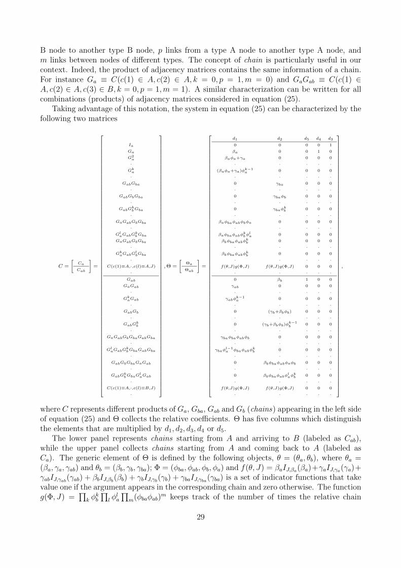
B node to another type B node, p links from a type A node to another type A node, andm links between nodes of different types. The concept of chain is particularly useful in ourcontext. Indeed, the product of adjacency matrices contains the same information of a chain.For instance Ga ≡ C(c(1) ∈ A, c(2) ∈ A, k = 0, p = 1,m = 0) and GaGab ≡ C(c(1) ∈A, c(2) ∈ A, c(3) ∈ B, k = 0, p = 1,m = 1). A similar characterization can be written for allcombinations (products) of adjacency matrices considered in equation (25).

Taking advantage of this notation, the system in equation (25) can be characterized by thefollowing two matrices

C =

[Ca

Cab

]=

Ia

Ga

G2a

·Gk

a

·GabGba

·GabGbGba

·GabG

kbGba

·GaGabGbGba

·Gl

aGabGkbGba

GaGabGbGba

·Gk

aGabGlbGba

·C(c(1)≡A,·,c(l)≡A,J)

·Gab

GaGab

·Gk

aGab

·GabGb

·GabG

kb

·GaGabGbGbaGabGba

·Gl

aGabGkbGbaGabGba

·GabGbGbaGaGab

·GabG

kbGbaG

laGab

·C(c(1)≡A,·,c(l)≡B,J)

·

,Θ =

[Θa

Θab

]=

d1 d2 d5 d4 d3

0 0 0 0 1

βa 0 0 1 0

βaφa+γa 0 0 0 0

· · · · ·(βaφa+γa)φk−1

a 0 0 0 0

· · · · ·0 γba 0 0 0

· · · · ·0 γbaφb 0 0 0

· · · · ·0 γbaφ

kb 0 0 0

· · · · ·βaφbaφabφbφa 0 0 0 0

· · · · ·βaφbaφabφ

kbφ

la 0 0 0 0

βbφbaφabφkb 0 0 0 0

· · · · ·βbφbaφabφ

kb 0 0 0 0

· · · · ·f(θ,J)g(Φ,J) f(θ,J)g(Φ,J) 0 0 0

· · · · ·0 βb 1 0 0

γab 0 0 0 0

· · · · ·γabφ

k−1a 0 0 0 0

· · · · ·0 (γb+βbφb) 0 0 0

· · · · ·0 (γb+βbφb)φk−1

b0 0 0

· · · · ·γbaφbaφabφb 0 0 0 0

· · · · ·γbaφ

l−1a φbaφabφ

kb 0 0 0 0

· · · · ·0 βbφbaφabφaφb 0 0 0

· · · · ·0 βbφbaφabφ

laφ

kb 0 0 0

· · · · ·f(θ,J)g(Φ,J) f(θ,J)g(Φ,J) 0 0 0

· · · · ·

,

where C represents different products of Ga, Gba, Gab and Gb (chains) appearing in the left sideof equation (25) and Θ collects the relative coefficients. Θ has five columns which distinguishthe elements that are multiplied by d1, d2, d3, d4 or d5.

The lower panel represents chains starting from A and arriving to B (labeled as Cab),while the upper panel collects chains starting from A and coming back to A (labeled asCa). The generic element of Θ is defined by the following objects, θ = (θa, θb), where θa =(βa, γa, γab) and θb = (βb, γb, γba); Φ = (φba, φab, φb, φa) and f(θ, J) = βaIJ,βa(βa)+γaIJ,γa(γa)+γabIJ,γab(γab) + βbIJ,βb(βb) + γbIJ,γb(γb) + γbaIJ,γba(γba) is a set of indicator functions that takevalue one if the argument appears in the corresponding chain and zero otherwise. The functiong(Φ, J) =

∏k φ

kb

∏l φ

la

∏m(φbaφab)

m keeps track of the number of times the relative chain

29

passes from one type of node to another scaled by the respective interaction parameters.Observe that (d1, d2, d3, d4, d5)′Θ′H∞ = 0 is equal to the condition E(Gaya)d1 +E(Gabyb)d2 +Xad3 +GaXad4 +GabXbd5 = 0. The elements of H∞ are equal to the elements of C multipliedby Xa or Xb depending on the last interaction matrix.47

From C and Θ one can argue that the model is identified in the cases listed in Proposition1.

Let us focus on case (2). For E(Za) to have full rank, it suffices that Θ has full rank. Thismeans that we need the linear independence of at least five chains (rows of C), translating tothe linear independence of Ia, Ga, G

2a, Gab and GabGb.

48 The corresponding five rows of Θare thus linear independent. Additionally we need to have five linear independent columns ofΘ, so having βaφa + γa 6= 0 and βbφb + γb 6= 0 suffices to reach the full rank condition for Θand consequently E(Za). The same argument applies for case (3).

Relationship with chains and trees. In the proof of Proposition 1 we have established theequivalence between sequences of products of adjacency matrices and the concept of chains.In order to provide a better intuition behind the multiple sufficient conditions argument notethat, according to the proof of Proposition 1 notation, a set of chains with a certain length pcan be divided in gp+1 number of chains, where g is the number of node types. For instance,chains of length 1 can be classified in four categories when nodes are split into two types.following proof notation we can define C(1) ≡ C(c(1) ≡ a, c(2) ∈ A, 0, 1, 0) ∪ C(c(1) ∈B, c(2) ∈ B, 1, 0, 0) ∪ C(c(1) ∈ A, c(2) ∈ B, 0, 0, 1) ∪ C(c(1) ∈ B, c(2) ≡ a, 0, 0, 1) (e.g.Ga ∪Gb ∪Gab ∪Gba = G).

We can see this system of chains as a tree, more specifically as a Tree-indexed Markovchain. A tree is a graph with a distinguished vertex x0 ∈ g (here a type A node, the startingpoint) and the degree of each vertex is at least two (in our case the number of types, g). Itsstructure is basically determined by a countable set of states (in our case the number of types,g) characterized by a transition probability ({p(x, y)|x, y ∈ g} in our case).49

Let Ta := ∪l,JC(c(1) ∈ A, ·, c(l), J) (Figure 3), it is simply the collection of all possiblechains of all possible lengths starting in a type A node. For identification purposes, we simplyneed that Ga, Gb, Gab and Gba are not empty (and not full).50 In words, it means that thereare no reasons why two randomly drawn nodes cannot be connected for each combination type(or that each node is connected with all of other nodes).51

47Note that H∞ is the IV matrix considered in Section 4, which is approximated by HK in the feasible 2SLSestimation.

48Note that here we need at least three chains from Ca and two from Cab because we are considering theoutcome equation for type A nodes, i.e. the staring point of chains is always a type A node.

49Given that here we are not interested in determining the transition probability law of a chain, even if it issimple to estimate and is basically the link formation probability considered for all of the possible combinationsof nodes’ type. Benjamini and Peres (1994) give a detailed discussion on Tree-indexed Markov chain.

50It is equivalent to say that the probability 0 < P (gij = 1) < 1, i ∈ A,B and j ∈ A,B. Note that transitionprobability can be derived from Ga, Gb, Gab and Gba. Here we are simply excluding the classical linear inmean framework (when the matrices are complete) and the case in which there are no connections (when thematrices are empty).

51From a Markov Chain perspective again, a more restrictive condition consists in assuming that the under-lying Markov Chain is irreducible and aperiodic. This means that type A are connected with type B or typeA with the same probability (and the same holds for type B). Thus, in this case tree branches with the samelength have the same probability of being observed. The aperiodicity and irreducibility are not necessary for

30

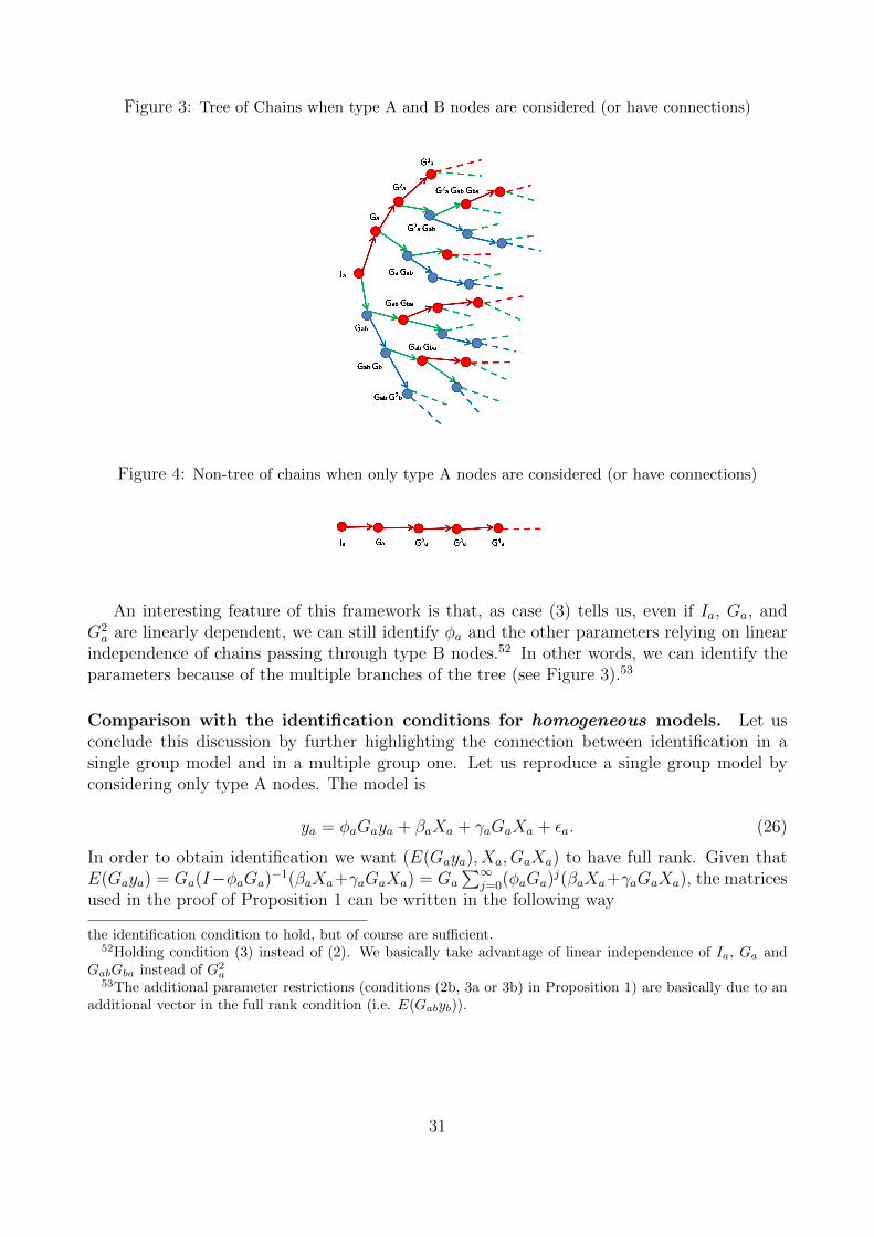
Figure 3: Tree of Chains when type A and B nodes are considered (or have connections)

Figure 4: Non-tree of chains when only type A nodes are considered (or have connections)

An interesting feature of this framework is that, as case (3) tells us, even if Ia, Ga, andG2a are linearly dependent, we can still identify φa and the other parameters relying on linear

independence of chains passing through type B nodes.52 In other words, we can identify theparameters because of the multiple branches of the tree (see Figure 3).53

Comparison with the identification conditions for homogeneous models. Let usconclude this discussion by further highlighting the connection between identification in asingle group model and in a multiple group one. Let us reproduce a single group model byconsidering only type A nodes. The model is

ya = φaGaya + βaXa + γaGaXa + εa. (26)

In order to obtain identification we want (E(Gaya), Xa, GaXa) to have full rank. Given thatE(Gaya) = Ga(I−φaGa)

−1(βaXa+γaGaXa) = Ga

∑∞j=0(φaGa)

j(βaXa+γaGaXa), the matricesused in the proof of Proposition 1 can be written in the following way

the identification condition to hold, but of course are sufficient.52Holding condition (3) instead of (2). We basically take advantage of linear independence of Ia, Ga and

GabGba instead of G2a

53The additional parameter restrictions (conditions (2b, 3a or 3b) in Proposition 1) are basically due to anadditional vector in the full rank condition (i.e. E(Gabyb)).

31

C =[Ca]

=

IaGa

G2a

·Gka

·

,Θ =[

Θa

]=

0 0 1βa 1 0

βaφa + γa 0 0· · ·

(βaφa + γa)φk−1a 0 0

· · ·

.

As before, these two matrices respectively represent the chains and their coefficients. Accord-ing to the proof of Proposition 1, the full rank condition for (E(Gaya), Xa, GaXa) depends onC and Θ. From C and Θ one can argue that the model is identified if (see proof of Proposition1 for details)

1. βaφa + γa 6= 0,

2. Ia, Ga and G2a are linear independent.

These are exactly the conditions of Proposition 1 in Bramoulle et al. (2009). Note thatif Ia, Ga and G2

a are linearly dependent, then Gka is also linearly dependent ∀k. Given that

here we cannot differentiate nodes, we have Ia ≡ C(0), Ga ≡ C(1), and G2a ≡ C(2), where

C(k) represent the set of chains with length k. In terms of chains it means that C(k) ≡{C(k − 1), C(1)} ≡ {C(k − 2), C(2)} ≡ · · · ≡ {C(2), C(k − 2)} ≡ {C(1), C(k − 1)}. In wordsit means that each chain’s set can be represented by at least two sets of chains. So each Gk

a

can be represented by the product of two matrices, GaGk−1a , G2

aGk−2a , and so on. This is the

connection to the linear independence of Ia, Ga, and G2a as a condition for identification. In

this case, a length l set of chains cannot be separated by node type, and thus Ta is composedonly of one chain (Figure 4) instead of multiple chains (Figure 3).54 Therefore, we need Ia,Ga, and G2

a to be linearly independent in order to have at least three independent chains inC and consequently identify the model’s parameters satisfying the restriction βaφa + γa 6= 0.

Proof of proposition 2. By the classical expansion the estimator is√n(µ − µ0) = 1

n(Z ′aPKZa)

−1 1√nZ ′aPKεa. As Za = fa + va, by Lemma 1 (v), we have

1n(Z ′aPKZa) = Fa + op(1). By Lemma 2 (iii) [Z ′aPKεa − σ2

a[e1, e2][tr(Ψa), φba(Ξba)]′]/√

(n) =

f ′aεa/√n+ op(1)

d→N(0, σ2aFa) by CLT.

Hence, the proposition is derived by Slutzky theorem

1

n(Z ′aPKZa)

−1 1√nZ ′aPKε

d→F−1a ·N(0, σ2

aFa) = N(0, σ2aF−1a ).

Proof of proposition 3. Given the proof of Proposition 2, it is sufficient to show that

σ2a[e1, e2][tr(Ψa), φba(Ξba)]

′/√n = op(1).

54Borrowing from Markov chains vocabulary again, this is because the state that characterizes the chain isonly one (A).

32

If we fix Ca, then by Lemma C.12 in Lee and Liu (2008) Ma −Ma = Ma(φa − φa)Ga +Ma((φabφba−φabφba)Ca). So we can write, tr(Ψa)−tr(Ψa) = tr(PK(Sa(φ)−Sa) = tr(PK(Ga(Ma−Ma) = tr(PK(Ga(Ma(φa − φa)Ga + Ma((φabφba − φabφba)Ca) = (φa − φa)tr(PK(Ga(MaGa) +(φbaφba − φabφba)tr(PK(Ga(MaCa)).

Since the product of UB matrices is still UB (Kelejian and Prucha 1998), using the lemmaB.2 (ii) in Lee and Liu (2010) and the initial

√n consistency assumption, we obtain√

n(φa−φa)tr(PK(Ga(MaGa)+√n(φbaφba−φabφba)tr(PK(Ga(MaCa))/n = op(1)O(K/n)+

op(1)O(K/n) = oP (K/n).

Finally, we have√n(σ2

a − σ2a)(tr(Ψa) − tr(Ψa))/n = op(1)op(K/n) = op(K/n) = oP (1) as

K/n → 0. The same procedure can be applied for√n(σ2

b − σ2b )(tr(Ξa) − tr(Ξa))/n and for

the second element of the stacked vector v.

Proof of proposition 4. Let p be a finite integer. Let us define the number of instrumentsequal to

K =P∑p=1

gp + o(1),

so that we have∑P

n=1 gp = O(gp). Since we assume K/n → 0, we have

∑Pp=1 g

p = o(n) by

assumption. This implies that gp = o(n). It follows that g = o(n1/p).

Proof of proposition 5. We prove this proposition for Ha(p)K . The same applies for H

b(p)K .

Let Θ(p)K be the matrix of true parameters derived from the p-order expansion of Θ (see Section

3). If sup‖φaGa‖∞ + sup‖φabφbaCa‖∞ < 1, then

H(p)K Θ

(p)K = Ga

p∑j=0

(φaGa + φabφbaCka )j(φabGabJbE(B)δb + E(A)δa).

It follows that ‖fa−H(p)K Θ

(p)K ‖∞ = ‖(φaGa + φabφbaC

ka )p+1Sa(φabGabJbE(B)δb +E(A)δa)‖∞ ≤

‖(φaGa + φabφbaCka )p+1‖∞‖Sa‖∞‖φabGabJbE(B)δb + E(A)δa‖∞ = o(1) as p→∞.

33

Appendix D: Tables and Figures

Table 1: Monte Carlo Simulation: 1000 obs., 1000 replications

(1) (2) (3)10 max connections 2SLS finite IVs 2SLS large IVs 2SLS bias-corrected

φa = 0.1 0.100(0.032) 0.100(0.026) 0.099 (0.027)φab = 0.2 0.201(0.031) 0.201(0.026) 0.197(0.069)βa = 0.5 0.501(0.047) 0.501(0.047) 0.501(0.048)γa = 0.5 0.503(0.081) 0.502(0.078) 0.503(0.076)γab = 0.5 0.496(0.079) 0.496(0.075) 0.500(0.097)

20 max connections 2SLS finite IVs 2SLS large IVs 2SLS bias-corrected

φa = 0.1 0.098(0.025) 0.098(0.020) 0.100(0.020)φab = 0.2 0.197(0.023) 0.195(0.019) 0.200(0.019)βa = 0.5 0.501(0.048) 0.501(0.048) 0.501(0.048)γa = 0.5 0.506(0.096) 0.506(0.093) 0.503(0.093)γab = 0.5 0.500(0.097) 0.497(0.093) 0.496(0.093)

30 max connections 2SLS finite IVs 2SLS large IVs 2SLS bias-corrected

φa = 0.1 0.099(0.020) 0.098(0.016) 0.099(0.016)φab = 0.2 0.198(0.019) 0.195(0.015) 0.199(0.015)βa = 0.5 0.500(0.048) 0.501(0.047) 0.501(0.047)γa = 0.5 0.506(0.110) 0.507(0.107) 0.505(0.107)γab = 0.5 0.500(0.112) 0.498(0.109) 0.497(0.109)Note: yb is generated with φb = 0.1, φba = 0.2, βb = 0.5, γb = 0.5, γba = 0.5

Table 2: Monte Carlo Simulation: 1000 obs., 1000 replications

(1) (2) (3)20 max connections 2SLS few IVs 2SLS many IVs 2SLS bias-corrected


20 max connections 2SLS few IVs 2SLS many IVs 2SLS bias-corrected


20 max connections 2SLS few IVs 2SLS many IVs 2SLS bias-corrected


34

Table 3: Monte Carlo Simulation: 1000 obs., 1000 replications, 10 max connections, φb =φab = φba = 0.3 ,βb = 0.5 ,γb = γab = γba = 0.5

2SLS/Misspeficied model 2SLS/misspecified IVs 2SLS/correct model-correct IVs

φa = 0.3 0.3684 (0.0335) 0.2971 (0.0465) 0.2999 (0.0164)βa = 0.5 0.3856 (0.1804) 0.4865 (0.2233) 0.5097 (0.1489)γa = 0.5 -0.0016 (0.2315) 0.4929 (0.2102) 0.4963 (0.1765)

Table 4: Monte Carlo Simulation: 1000 obs., 1000 replications, 10 max connections

(1) (2) (3)φa = φb = φba = φab = 0.1 φa = φb = 0.1 ,φba = φab = 0.3 φa = 0.1, φb = 0.2, φba = 0.05 , φab = 0.4

φ 0.100(0.020) 0.178(0.021) 0.205(0.022)β 0.500(0.031) 0.499(0.034) 0.499(0.033)γ 0.446(0.022) 0.445(0.024) 0.442(0.025)

Figure 5: Policy experiment: varying φa and φab

35

Figure 6: Policy experiment: varying φa and φba

Figure 7: Kernel density estimation of empirical distributions of ∆yi∈A and ∆yi∈B, increasing φa.

36

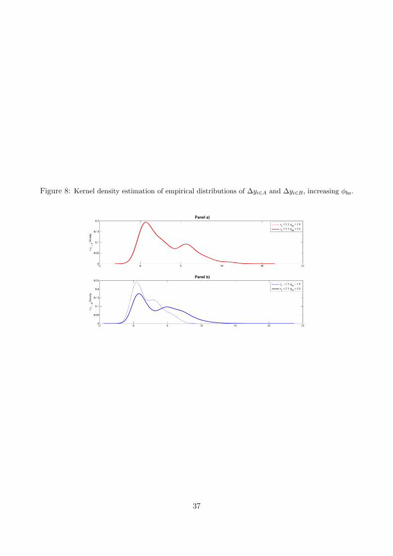
Figure 8: Kernel density estimation of empirical distributions of ∆yi∈A and ∆yi∈B, increasing φba.

37

Identification and Estimation of Outcome Response with Heterogeneous Treatment Externalities

Documents

Transcript of Identification and Estimation of Outcome Response with Heterogeneous Treatment Externalities