Advanced Robotics 26 (2012) 487–514brill.nl/ar

Full paper

Comparison of Two Sequencing Techniques to Perform aVision-Based Navigation Task in a Cluttered Environment

Viviane Cadenat a,b,∗, David Folio c and Adrien Durand Petiteville a,b

a CNRS, LAAS, 7, avenue du Colonel Roche, F-31077 Toulouse Cedex 4, Franceb Université de Toulouse, UPS, INSA, INP, ISAE, UT1, UTM, LAAS, F-31077 Toulouse Cedex 4,

Francec Laboratoire PRISME, Ecole Nationale Superieur d’Ingenieurs de Bourges, 88 Boulevard Lahitolle,

F-18020 Bourges, France

Received 14 January 2011; accepted 1 March 2011

AbstractWe address the problem of multi-sensor-based navigation in a cluttered environment for a non-holonomicrobot. To perform such a successful and safe navigation, three controllers realizing, respectively, nominalvision-based navigation, obstacle bypassing and occlusion avoidance have been designed using the taskfunction approach. Then it suffices to sequence them to realize the complete mission. To guarantee thecontrol continuity when switching between two successive controllers, two sequencing approaches havebeen used and compared. Simulation results validate our work.© Koninklijke Brill NV, Leiden and The Robotics Society of Japan, 2012

KeywordsTask sequencing, visual servoing, obstacle avoidance, occlusion avoidance, task function

1. Introduction

Visual servoing techniques aim at controlling robot motion using vision data pro-vided by a camera to reach a desired goal defined in the image [1]. Therefore, thesetechniques cannot be used if these features are lost during the robotic task. Theidea is then to use methods allowing us to preserve the visibility of visual featuresduring the whole execution of the mission. Most of them are dedicated to manip-ulator arms and propose to treat this kind of problem by using redundancy [2, 3],path planning [4], specific degrees of freedom (d.o.f.) [5, 6], zoom [7] or even bymaking a tradeoff with the nominal vision-based task [8].

* To whom correspondence should be addressed. E-mail: cadenat@laas.fr

© Koninklijke Brill NV, Leiden and The Robotics Society of Japan, 2012 DOI:10.1163/156855311X617470

488 V. Cadenat et al. / Advanced Robotics 26 (2012) 487–514

In a mobile robotics context, the issue is slightly different. Indeed, first of all,the successful realization of a vision-based navigation task in a cluttered environ-ment requires us to preserve not only image data visibility, but also robot safety.Therefore, there is an additional objective with respect to the manipulator arm case.Furthermore, the number of available d.o.f. may be reduced and the use of redun-dancy is then more difficult. In our case, the considered robot is a non-holonomicvehicle equipped with an ultrasonic (US) sensor belt and a camera mounted on apan platform. Only 3 d.o.f. are then available; redundancy will, thus, be very lim-ited. In this work, we aim at designing a sensor-based control law allowing us tofulfill the two previously mentioned objectives — non-collision and landmark non-occlusion. The proposed control strategy is the sequel to previous works [9, 10]. Itconsists in a three-step method: (i) the navigation task is split into several subtasksto be sequenced, (ii) then a separate controller allowing us to realize each subtaskis designed and finally (iii) the global control law is deduced by sequencing them.The implementation of such a control strategy requires a smooth transition betweenthe different controllers. The literature provides two different approaches able toguarantee the global control law continuity. In the first approach, the controllersare merged using a simple convex combination based on time as in Ref. [11] oron parameters characterizing the risks of occlusions and collisions as in Refs [9,10]. In the second approach, the controllers are dynamically sequenced (i.e., thecontrol law is designed so that it is naturally smooth when the switch occurs). Fewworks use this second approach as it is a bit more difficult to handle than the firstone. We may nonetheless mention the work by Souères and Cadenat who first pro-posed a formalism dedicated to dynamical sequencing and applied it to merge twocontrollers to perform a complex navigation task [12]. The same formalism wasthen used by Gao to improve the robotic task execution by dynamically sequenc-ing multi-criteria visual-servoing controllers [13]. However, for these two cases, theswitch depends on time and not on relevant events, such as an occlusion or a colli-sion. Thus, an important part of this work will be devoted to the choice of switchingconditions. Finally, let us also note that dynamical sequencing has been also usedfor manipulator arms and humanoid robots to switch smoothly between differentsecondary tasks [14]. However, as previously mentioned, the issue is rather differ-ent because the proposed approach strongly benefits from the redundancy with anumber of available d.o.f. considerably larger than in our case.

In this paper, we deal with the problem of executing a vision-based navigationtask amidst possibly occluding obstacles. The proposed control strategy relies onthe continuous switch between three controllers, respectively, realizing nominalvision-based task, obstacle bypassing and occlusion avoidance. The transition isperformed using two different methods, respectively, based on convex combinationand dynamical sequencing. These two approaches are then analyzed and compared.

This paper is organized as follows. Sections 2 and 3 are dedicated to problemmodeling and control issues. The obtained simulation results and a comparative

V. Cadenat et al. / Advanced Robotics 26 (2012) 487–514 489

analysis are presented in Section 4. Section 5 presents the conclusions and futurework.

2. Problem Modeling

We first describe the robotic system before modeling the three above-mentionedsubtasks — the nominal vision-based task, occlusion avoidance and collision avoid-ance.

2.1. Robotic System

We first model our robotic system to characterize the camera kinematic screw T c.To this aim, considering Fig. 1a, we define the successive frames: FM (M,

−→x M,−→y M,

−→z M ) linked to the robot, FP (P,−→x P ,

−→y P ,−→z P ) attached to the pan platform

and FC (C,−→x C,

−→y C,−→z C) linked to the camera. Let ϑ be the direction of the pan

platform with respect to −→x M ; where P is the pan platform center of rotation, andDx is the distance between the robot reference point M and P . The control input isdefined by q = (v,ω,�)T, where v and ω are the cart linear and angular velocities,and � is the pan platform angular velocity with respect to FM . The kinematic screwT c is related to the control input by the robot Jacobian J: T c = Jq . As the camerais constrained to move horizontally, it is sufficient to consider a reduced kinematicscrew T c

r = (V−→y C, V−→z C

, �−→x C)T and a reduced Jacobian matrix Jr as:

T cr =

(V−→y C

V−→z C

�−→x C

)=

(− sin(ϑ) Dx cos(ϑ) + Cx Cx

cos(ϑ) Dx sin(ϑ) − Cy −Cy

0 −1 −1

)(v

ω

�

)= Jr q, (1)

where Cx and Cy are the coordinates of C along axes −→x P and −→y P (Fig. 1). Noticethat Jr is a regular matrix as det (Jr) = Dx �= 0.

(a) (b)

Figure 1. System modeling. (a) Cart-like robot with a camera mounted on a pan-platform. (b) Thepinhole camera model.

490 V. Cadenat et al. / Advanced Robotics 26 (2012) 487–514

2.2. Sensor-Based Model

Recalling that our goal is to realize a vision-based navigation task with respect toa static landmark, we denote by s a set of relevant visual data characterizing thislandmark and by z a vector describing its depth (Fig. 1b). The focal length f issupposed to be equal to 1 as in Ref. [15]. For a fixed landmark, the variation ofthe visual signal s is related to the camera kinematic skrew T c

r by means of theinteraction matrix L(s,z) as [15]:

s = L(s,z) T cr . (2)

L(s,z) allows to relate the visual features motion in the image to the three-dimensional camera motion. It depends mainly on the depth z (which is not alwaysavailable online) and on the considered visual data. Expressions of L(s,z) are avail-able for different kinds of features, such as points, straight lines, circles [15], imagemoments [16], etc.

2.3. Vision-Based Task

Here, we only consider the nominal vision-based navigation task to be performed.The goal of the considered task is to position the embedded camera with respect toa fixed landmark. To this aim, we have applied the visual servoing technique givenin Ref. [15] to mobile robots as in Ref. [11]. The proposed approach relies on thetask function formalism [17]. This formalism deals with a special kind of outputfunctions called task functions. The idea is to characterize the desired mission bya suitable task function e(q(t)) so that its regulation to zero leads to a successfulexecution of the task. A sufficient condition that guarantees the control problemto be well conditioned is that e is admissible. Indeed, this property ensures theexistence of a diffeomorphism between the task space and the space of generalizedcoordinates Q, so that the ideal trajectory q�(t) corresponding to e(q�(t)) = 0 isunique. This condition is fulfilled if ∂ e(q(t))

∂qis regular around q�(t) [17]. Using

the task function formalism, the visual servoing task is classically defined as theregulation of the following error function to zero [1]:

evs = L+(s�)(s − s�), (3)

where s� is the visual features desired value and L+ denotes the matrix interactionpseudo-inverse.

2.4. Occlusion Avoidance Task

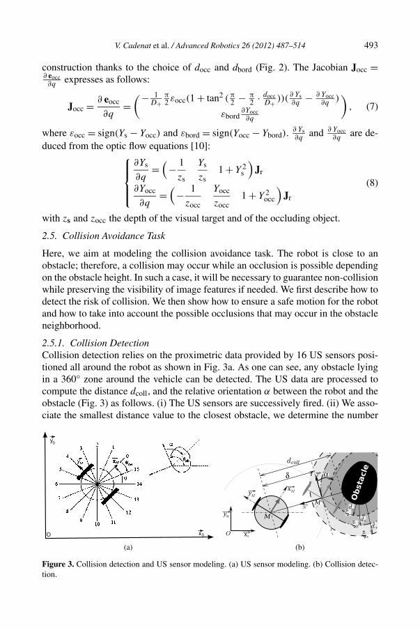
Now, we consider that only occlusions can occur — an occluding object can enterthe camera field of view to temporarily hide the image features, but is too far toinduce a collision risk. Our goal is to define the occlusion avoidance task functionso that the image features visibility is preserved along the execution of the mission.We first describe the way we determine the occlusion before defining a suitable taskfunction.

V. Cadenat et al. / Advanced Robotics 26 (2012) 487–514 491

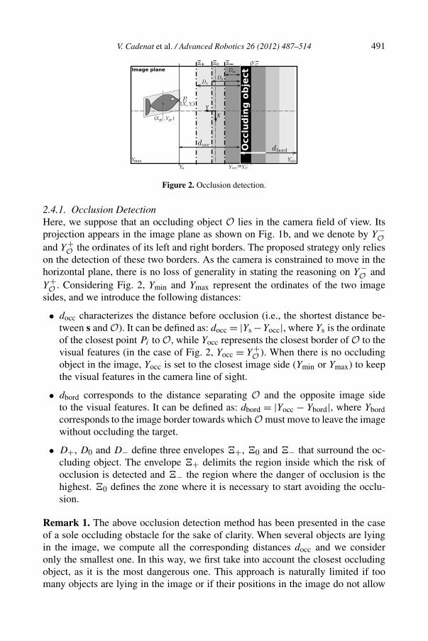
Figure 2. Occlusion detection.

2.4.1. Occlusion DetectionHere, we suppose that an occluding object O lies in the camera field of view. Itsprojection appears in the image plane as shown on Fig. 1b, and we denote by Y−

Oand Y+

O the ordinates of its left and right borders. The proposed strategy only relieson the detection of these two borders. As the camera is constrained to move in thehorizontal plane, there is no loss of generality in stating the reasoning on Y−

O andY+

O . Considering Fig. 2, Ymin and Ymax represent the ordinates of the two imagesides, and we introduce the following distances:

• docc characterizes the distance before occlusion (i.e., the shortest distance be-tween s and O). It can be defined as: docc = |Ys −Yocc|, where Ys is the ordinateof the closest point Pi to O, while Yocc represents the closest border of O to thevisual features (in the case of Fig. 2, Yocc = Y+

O ). When there is no occludingobject in the image, Yocc is set to the closest image side (Ymin or Ymax) to keepthe visual features in the camera line of sight.

• dbord corresponds to the distance separating O and the opposite image sideto the visual features. It can be defined as: dbord = |Yocc − Ybord|, where Ybordcorresponds to the image border towards which O must move to leave the imagewithout occluding the target.

• D+, D0 and D− define three envelopes �+, �0 and �− that surround the oc-cluding object. The envelope �+ delimits the region inside which the risk ofocclusion is detected and �− the region where the danger of occlusion is thehighest. �0 defines the zone where it is necessary to start avoiding the occlu-sion.

Remark 1. The above occlusion detection method has been presented in the caseof a sole occluding obstacle for the sake of clarity. When several objects are lyingin the image, we compute all the corresponding distances docc and we consideronly the smallest one. In this way, we first take into account the closest occludingobject, as it is the most dangerous one. This approach is naturally limited if toomany objects are lying in the image or if their positions in the image do not allow

492 V. Cadenat et al. / Advanced Robotics 26 (2012) 487–514

us to realize the navigation task while avoiding occlusions. In such a case, the robotwill be stopped to preserve its safety. Other approaches consisting in toleratingocclusions must then be used (e.g., see Ref. [18]).

2.4.2. Task Function DesignThe redundant task function formalism consists of defining a redundant task e1,which is a low-dimensioned task that does not constrain all the robot d.o.f. The ideais to benefit from this redundancy to perform an additional objective. The lattercan be modeled as a cost function h to be minimized under the constraint thate1 is perfectly performed. The resolution of this optimization problem leads us toregulate the following global task [17]:

e = W+e1 + β(I − W+W)g, (4)

where W+ = WT(WWT)−1, g = ∂ h∂q

and β > 0. Under some assumptions, whichare verified if W = ∂ e1

∂q, the task Jacobian ∂ e

∂qis positive-definite around the ideal

trajectory q�(t), ensuring that e is admissible [17].Our objective is to apply these theoretical results to avoid occlusions while keep-

ing the target in the image. We have chosen to define the occlusion avoidance asthe prioritary task. The target tracking will then be considered as the secondaryobjective and will be modeled as a criterion hs to be minimized. We propose thefollowing occlusion avoidance (oa) task function:

eoa = J+occeocc + βoa

(I − J+

occJocc)gs, (5)

where eocc represents the redundant task function allowing us to avoid the occlu-sions, Jocc = ∂ eocc

∂q, and βoa > 0 and gs = ∂ hs

∂qare as explained above. We propose

the following criterion to track the target and keep it in the line of sight of the cam-era: hs = 1

2(s − s∗)T(s − s∗). Its gradient is then given by: gs = ((s − s∗)TL(s)Jr)T.

Now, let us define the prioritary task function eocc to avoid occlusions. We proposethe following redundant task function:

eocc =(

tan (π2 − π

2 · doccD+ )

dbord

). (6)

The first component allows us to avoid target occlusions: it increases when theoccluding object gets closer to the visual features and becomes infinite when docctends to zero. On the contrary, it decreases when the occluding object is moving farfrom the visual features and vanishes when docc equals D+. Note that, ∀docc � D+,eocc is maintained to zero. The second component makes the occluding object goout of the image, which is realized when dbord vanishes. Let us remark that thesetwo tasks must be compatible (i.e., they can be simultaneously realized) in orderto guarantee the control problem to be well stated. This condition is fulfilled by

V. Cadenat et al. / Advanced Robotics 26 (2012) 487–514 493

construction thanks to the choice of docc and dbord (Fig. 2). The Jacobian Jocc =∂ eocc∂q

expresses as follows:

Jocc = ∂ eocc

∂q=

(− 1D+

π2 εocc(1 + tan2 (π

2 − π2 · docc

D+ ))( ∂ Ys∂q

− ∂ Yocc∂q

)

εbord∂Yocc∂q

), (7)

where εocc = sign(Ys − Yocc) and εbord = sign(Yocc − Ybord).∂ Ys∂q

and ∂ Yocc∂q

are de-duced from the optic flow equations [10]:⎧⎪⎪⎨

⎪⎪⎩∂Ys

∂q=

(− 1

zs

Ys

zs1 + Y 2

s

)Jr

∂Yocc

∂q=

(− 1

zocc

Yocc

zocc1 + Y 2

occ

)Jr

(8)

with zs and zocc the depth of the visual target and of the occluding object.

2.5. Collision Avoidance Task

Here, we aim at modeling the collision avoidance task. The robot is close to anobstacle; therefore, a collision may occur while an occlusion is possible dependingon the obstacle height. In such a case, it will be necessary to guarantee non-collisionwhile preserving the visibility of image features if needed. We first describe how todetect the risk of collision. We then show how to ensure a safe motion for the robotand how to take into account the possible occlusions that may occur in the obstacleneighborhood.

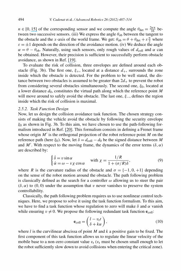
2.5.1. Collision DetectionCollision detection relies on the proximetric data provided by 16 US sensors posi-tioned all around the robot as shown in Fig. 3a. As one can see, any obstacle lyingin a 360° zone around the vehicle can be detected. The US data are processed tocompute the distance dcoll, and the relative orientation α between the robot and theobstacle (Fig. 3) as follows. (i) The US sensors are successively fired. (ii) We asso-ciate the smallest distance value to the closest obstacle, we determine the number

(a) (b)

Figure 3. Collision detection and US sensor modeling. (a) US sensor modeling. (b) Collision detec-tion.

494 V. Cadenat et al. / Advanced Robotics 26 (2012) 487–514

n ∈ [0,15] of the corresponding sensor and we compute the angle θdet = 2nπ16 be-

tween two successive sensors. (iii) We express the angle θob between the tangent tothe obstacle and the x-axis of the world frame. We get: θob = θ + θdet + επ

2 whereε = ±1 depends on the direction of the avoidance motion. (iv) We deduce the angleα = θ − θob. Naturally, using such sensors, only rough values of dcoll and α canbe obtained. However, their precision is sufficient to successfully perform obstacleavoidance, as shown in Ref. [19].

To evaluate the risk of collision, three envelopes are defined around each ob-stacle (Fig. 3b). The first one, ξ+, located at a distance d+, surrounds the zoneinside which the obstacle is detected. For the problem to be well stated, the dis-tance between two obstacles is assumed to be greater than 2d+ to prevent the robotfrom considering several obstacles simultaneously. The second one, ξ0, located ata lower distance d0, constitutes the virtual path along which the reference point M

will move around to safely avoid the obstacle. The last one, ξ−, defines the regioninside which the risk of collision is maximal.

2.5.2. Task Function DesignNow, let us design the collision avoidance task function. The chosen strategy con-sists of making the vehicle avoid the obstacle by following the security envelopeξ0 as shown in Fig. 3b. To this aim, we have chosen to use the path-following for-malism introduced in Ref. [20]. This formalism consists in defining a Frenet framewhose origin M ′ is the orthogonal projection of the robot reference point M on thereference path (here ξ0). Now, let δ = dcoll − d0 be the signed distance between M

and M ′. With respect to the moving frame, the dynamics of the error terms (δ,α)

are described by: {δ = v sinα

α = ω − vχ cosαwith χ = 1/R

1 + (σ/R)δ, (9)

where R is the curvature radius of the obstacle and σ = {−1,0,+1} dependingon the sense of the robot motion around the obstacle. The path following problemis classically defined as the search for a controller ω allowing us to steer the pair(δ,α) to (0,0) under the assumption that v never vanishes to preserve the systemcontrollability.

Classically, the path following problem requires us to use nonlinear control tech-niques. Here, we propose to solve it using the task function formalism. To this aim,we have to find a task function whose regulation to zero will make δ and α vanishwhile ensuring v �= 0. We propose the following redundant task function ecoll:

ecoll =(

l − vrt

δ + kα

), (10)

where l is the curvilinear abscissa of point M and k a positive gain to be fixed. Thefirst component of this task function allows us to regulate the linear velocity of themobile base to a non-zero constant value vr (vr must be chosen small enough to letthe robot sufficiently slow down to avoid collisions when entering the critical zone).

V. Cadenat et al. / Advanced Robotics 26 (2012) 487–514 495

In this way, the linear velocity never vanishes, guaranteeing that the control prob-lem is well stated and that the robot will not remain stuck on the security envelopeξ0 during the obstacle avoidance. The second component of ecoll can be seen as asliding variable whose regulation to zero makes both δ and α vanish (see Ref. [21]for a detailed proof). The value of k determines the relative convergence velocity ofδ and α as the sliding variable converges. Therefore, the regulation to zero of ecollguarantees that the robot follows the security envelope ξ0, ensuring non-collision.As the chosen task function does not constrain the whole d.o.f. of the robot, we usethe redundant task function formalism to perform a secondary task (here, avoidingtarget loss and occlusions at best) while the obstacle avoidance is realized. We pro-pose to model this secondary objective using the cost function: hocc = 1

docc. Thus,

the collision avoidance (ca) task function eca expresses as:

eca = J+collecoll + βca(I − J+

collJcoll)gocc, (11)

where βca > 0 and the gradient gocc is given by gocc = ∂hocc∂q

= − 1d2

occ

∂docc∂q

=− εocc

d2occ

( ∂Ys∂q

− ∂Yocc∂q

)T. Finally, a straightforward calculus shows that the task Jaco-

bian Jcoll is given by:

Jcoll = ∂ecoll

∂q=

(1 0 0

sinα − kχ cosα k 0

). (12)

3. Control Design

At this step, three task functions have been designed: the first, evs (3), models thenominal vision-based task in the free space, the second, eoa (5), treats the occlu-sions generated by obstacles located far from the robot, and the third, eca (11),handles collision problems while avoiding occlusions if needed. Now, it remainsto determine three controllers allowing us to regulate them to zero and to select aconvenient sequencing technique. In fact, these two problems are closely relatedbecause the control law discontinuity at the switching instant comes from the sepa-rate computation of the controllers to be sequenced. As mentioned in Section 1, twokinds of methods may be used to suppress it: either the different controllers are in-dependently designed and then the global control law smoothness is ensured thanksto convex combination [9–11] or the smoothness constraint is directly taken intoaccount in the design step so that the obtained control law is naturally continuous[12–14]. We successively consider these two different approaches.

3.1. Convex Combination

In this case, the controllers are merged thanks to convex combinations depending ontime [11] or on parameters that significantly characterize the task execution [9, 10].Therefore, when using such techniques, the global control law smoothness onlydepends on the convex combination parameters. The controllers to be sequencedcan then be separately designed, using any convenient dynamics, provided that it

496 V. Cadenat et al. / Advanced Robotics 26 (2012) 487–514

allows us to guarantee that the considered task functions will be efficiently regu-lated to zero. In this work, we have applied classical results from the literature todetermine the three desired controllers. We briefly describe the design techniquesfor each subtask before proposing a global control strategy.

3.1.1. Design of the Controllers to be Sequenced• Visual servoing controller. To make evs vanish, a classical solution consists of

imposing an exponential decrease, i.e., evs = −γvsevs, where γvs is a positivescalar or a positive definite matrix [1]. The visual servoing controller can thenbe written as:

qvs = (L+(s�)L(s)Jr)

−1(−γvs)evs. (13)

Note that, as Jr is a regular matrix, the stability of this control scheme is mainlyrelated to the positivity of L(s)L

+(s�) and that the admissibility of the task requires

that this product remains always invertible [1].

• Occlusion avoidance controller. Now, we address the occlusion avoidance con-troller determination. Our goal is then to design a controller allowing us toregulate task function eoa to zero by imposing an exponential decay. As Joccand βoa are chosen to fulfill the assumptions of the redundant task formalism[17], the task Jacobian Joa = ∂ eoa

∂ qis positive definite around q�(t) and eoa is

admissible. This result allows us to simplify the control synthesis, as it can beshown that a controller making eoa vanish is given by [15]:

qoa = −γoaeoa, (14)

where γoa is a positive scalar or a positive definite matrix.

• Collision avoidance controller. Here, we consider the problem of designing acontrol law able to drive safely the robot in the obstacle vicinity. Using the sameprevious reasoning to regulate eca to zero, we obtain:

qca = −γcaeca, (15)

where γca is a positive scalar or a positive definite matrix.

Remark 2. As controllers (14) and (15) are computed by approximating Joa andJca, the exponential decrease is lost. Indeed, it can be shown that the closed-loopevolutions of eoa and eca are expressed by:

eoa = −JoaJ−1oa γoaeoa and eca = −JcaJ−1

ca γcaeca, (16)

where Joa and Jca correspond to the approximations of Joa and Jca. When Joa =Jca = Id, stability is preserved only if Joa and Jca are positive definite. This lastcondition is verified if the assumptions of the redundant task function formalismare fulfilled [17], which is the case in our work. A detailed proof can be found inRef. [15].

V. Cadenat et al. / Advanced Robotics 26 (2012) 487–514 497

3.1.2. Global Control Law DesignAt this step, the controllers allowing us to perform the three desired subtasks havebeen designed. Now, it remains to select the right one depending on the environment(i.e., depending on the risk of collisions and/or occlusions). To this aim, we use aconvex combination and we propose the following global control law:

q = (1 − μcoll)[(1 − μocc)qvs + μoccqoa] + μcollqca, (17)

where qvs, qoa and qca are, respectively, given by (13), (14) and (15). μocc andμcoll ∈ [0,1] allow us to switch continuously from one control to the other depend-ing on the risk of occlusion and of collision. As one can see, the proposed strategyguarantees that the collision avoidance is performed as a priority, guaranteeing therobot safety. Several cases may occur:

• If there is no occluding object O in the neighborhood of the visual features s(docc > D0) and no obstacle in the vicinity of the vehicle (dcoll > d0), μocc andμcoll are fixed to 0 and the sole visual control qvs is used.

• If the visual features s enter the zone delimited by �0 (docc < D0), the dangerof occlusion becomes higher and μocc progressively increases to reach 1 whenthey cross �−. Therefore, while the visual features remain between �0 and �−,the robot is controlled by a linear combination of qvs, qoa and possibly qca (seeRemark 3). If the action of the global controller is sufficient to avoid the oc-clusions, the visual features may naturally leave the critical zone defined by �0and μocc goes back to 0 without having reached 1. On the contrary, once �− iscrossed, μocc is maintained to 1 until O leaves the image (dbord = 0) or at leastgoes out of the critical zone (docc > D0) (i.e., the risk of occlusion is consideredto be sufficiently reduced). Therefore, the leaving condition is obtained wheneither dbord = 0 or docc = D0. When one of these two events occurs, μocc is pro-gressively reduced from 1 to 0 and vanishes once the visual features cross �+.Following this reasoning, μocc depends on the distance between the occludingobject and the visual features in the image (i.e., docc).

• If the mobile base enters the zone surrounded by ξ0 (dcoll < d0), the danger ofcollision rises and μcoll is continuously increased from 0 to reach 1 when dcoll <

d−. If ξ− is never crossed, the robot naturally leaves the critical zone definedby ξ0 and μcoll is brought back to 0, once ξ+ is crossed. If μcoll reaches 1, thecollision risk is maximum and a flag AVOID is enabled. As the robot safetyis considered to be the most important objective, the global controller (17) hasbeen designed so that only qca is applied to the vehicle once μcoll is set to 1.In this way, the robot is controlled using the sole controller qca, allowing us toguarantee non-collision while performing the occlusion avoidance at best. Therobot is then brought back on the security envelope ξ0 and follows it until theobstacle is overcome. This event occurs when the camera and the mobile basehave the same direction θ = ϑ . A flag LEAVE is then positioned to 1 and μcollis rapidly decreased to vanish on ξ+.

498 V. Cadenat et al. / Advanced Robotics 26 (2012) 487–514

Table 1.Switching strategy

μocc = 0 μocc ∈]0,1[ μocc = 1

μcoll = 0 q = qvs qvs ↔ qoa q = qoaμcoll ∈]0,1[ qvs ↔ qca q = f (qvs, qoa, qca) qoa ↔ qcaμcoll = 1 q = qca q = qca q = qca

Remark 3. The different envelopes are chosen close enough in order to reduce theduration of the transition phase and ensure that the robot will be rapidly controlledby the most relevant controller depending on the environment.

Naturally, μcoll and μocc can be defined by any expression satisfying the previousconstraints. A possible choice is given as [10]:⎧⎪⎪⎪⎪⎪⎪⎪⎪⎪⎪⎨

⎪⎪⎪⎪⎪⎪⎪⎪⎪⎪⎩

μocc = 0 if docc > D0 and OCCLU = 0

μocc = docc − D0

D− − D0if docc ∈ [D−,D0] and OCCLU = 0

μocc = docc − D+D0 − D+

if docc ∈ [D0,D+] and docc = D0

μocc = docc − D+Dl − D+

if docc ∈ [Dl,D+] and (dbord = 0 or docc � D0)

μocc = 1 otherwise,

(18)

where OCCLU is the flag indicating that μocc has reached its maximal value 1and Dl is the value of the distance docc for which the leaving condition has beenfulfilled. As for μcoll, we propose the following definition [10]:⎧⎪⎪⎪⎪⎪⎪⎨

⎪⎪⎪⎪⎪⎪⎩

μcoll = 0 if (dcoll > d0) and AVOID = 0 and LEAVE = 0

μcoll = dcoll − d0

d− − d0if dcoll ∈ [d−, d0] and AVOID = 0

μcoll = dcoll − d+dl − d+

if dcoll ∈ [dl, d+] and LEAVE = 1

μcoll = 1 otherwise,

(19)

where dl is defined by the distance dcoll when leave = 1. The switching strategy issummarized in Table 1.

3.2. Dynamical Sequencing

As previously explained, the control law discontinuity at the switching instant ariseswhen the controllers to be sequenced are separately computed. In the above solu-tion, the smoothness is a posteriori imposed thanks to a convex combination. Here,the idea is to propose a method allowing us to naturally obtain a continuous controllaw at the switching time. It is then necessary to guarantee that the values of the

V. Cadenat et al. / Advanced Robotics 26 (2012) 487–514 499

two successive controllers are identical at this time. Souères and Cadenat have pro-posed a formalism allowing us to fulfill this particular property [12]. We first brieflydescribe this formalism before applying it in our specific case.

3.2.1. Sequencing FormalismThis formalism relies on the admissibility property. As previously mentioned, thisproperty allows us to define a local diffeomorphism between the task space andthe generalized coordinates space Q. Souères and Cadenat have shown that it canalso be used to define a structure of differential manifold on Q [12]. The evolutionof the next task induced by the execution of the current task can then be uniquelyexpressed. From this result, it is possible to deduce a controller able to take intoaccount the constraints on the evolutions of the two tasks to be sequenced at theswitching time. The control law smoothness can then be guaranteed. Hereafter, weonly present the general reasoning. Theoretical aspects can be found in Ref. [12].We consider two tasks to be sequenced. We assume that they can be modeled by twoadmissible task functions e1(q(t)) and e2(q(t)), which implies that their Jacobianmatrices J1 = J1(q(t)) = ∂e1

∂qand J2 = J2(q(t)) = ∂e2

∂qare invertible. Derivating

e1(q(t)) and e2(q(t)) with respect to time leads to the following natural result:

e1 = e1(q(t)) = J1q and e2 = e2(q(t)) = J2q. (20)

Now, we assume that the goal consists of executing first e1 and then e2. To thisaim, we design a kinematic controller q so that e1 is regulated to zero. Using (20)and recalling that J1 is invertible, the desired controller is given by:

q = J−11 e∗

1, (21)

where e∗1 = e∗

1(q(t)) is the chosen dynamics to make e1 vanish. Following the samereasoning, we can also design a controller to perform the second task. We obtain:

q = J−12 e∗

2, (22)

where e∗2 = e∗

2(q(t)) is the dynamics imposed to regulate e2 to zero.Thus, executing first e1 and then e2 requires us to switch continuously between

controllers (21) and (22). As the dynamics of e1 has been already fixed to realizethe first task the best way, the only parameter that can be tuned to ensure the globalcontrol law smoothness is the dynamics of e2, namely e∗

2. The key idea consists thenin choosing e∗

2 so that the continuity is preserved at the switching instant t = ts. Tothis aim, it is necessary to evaluate the effect of the execution of task e1 on thedynamics of e2 at t = ts. Using (20) and taking into account that q is given byrelation (21) when the first task is performed, we obtain:

e2(q(t)) = J2q = J2 J−11 e∗

1(q(t)). (23)

Thus, the global control law continuity will be insured if e∗2 is chosen so that rela-

tion (23) is verified at t = ts. Finally, the global control law is given by:

q(t) ={

J−11 e∗

1(q(t)) ∀t � ts

J−12 e∗

2(q(t)) ∀t � ts,(24)

500 V. Cadenat et al. / Advanced Robotics 26 (2012) 487–514

where e∗2(q(t)) is computed so that its value at the switching instant is given by

relation (23) expressed at t = ts. Therefore, this relation provides the conditionthat must be verified by the second task dynamics for the controller to be contin-uous. More details about the theoretical foundations of this result can be found inRef. [12].

3.2.2. Chosen DynamicsNow, it remains to impose a suitable dynamics for e2. Following the previous rea-soning, the dynamics e∗

2 must be chosen so that:

(i) The task function e2 is regulated to zero, which allows us to successfully per-form the mission.

(ii) The value of e∗2(q(ts)) can be imposed to verify (23) at t = ts, guaranteeing the

control law smoothness at the switching time.

Therefore, a simple classical exponential decay does not fulfill the second require-ment as it does not allow us to constrain the value of e∗

2 at t = ts. Another solution,suggested by Souères and Cadenat in Ref. [12], is to use a second-order linear dy-namics:

e2 + k1e2 + k2e2 = 0, (25)

where the two parameters k1 > 0 and k2 > 0 are used to control both the errordecreasing speed and the duration of the transient time response. Although this dy-namics satisfies the two previous objectives, it may be difficult to choose the valuesof these parameters to obtain a convenient behavior. This is the reason why Mansardand Chaumette propose to use a nonhomogeneous first-order dynamics [14]:

e∗2(q(t)) = −λe2(q(t)) + ρ(t), (26)

where ρ(t) = κe−τ(t−ts) with κ given by:

κ = e2(q(ts)) + λe2(q(ts)) = J2(q(ts))J−11 (q(ts))e∗

1(q(ts)) + λe2(q(ts)), (27)

λ > 0 and τ > 0 represent two gains which allow us to set independently the errordecreasing speed and the transient time duration (in order to ensure a short tran-sient time response with respect to the decreasing time of the task error, it sufficesto choose τ > λ [14]). Note that the above dynamics is equivalent to the one de-signed by Souères and Cadenat [12] if k1 = λ + τ and k2 = λτ . Therefore, the twoapproaches are equivalent, except that the latter offers the advantage of discouplingthe error decreasing speed from the transient time duration.

Now, it remains to verify that the proposed dynamics (26) allows us to satisfy thetwo previously mentioned requirements. To this aim, let us analyze its behavior atthe switching time ts. Two cases may occur:

• At t = ts: it is straightforward to show that the necessary initial condition on e∗2

is obtained at this instant, because relation (26) can be rewritten as e∗2(q(ts)) =

J2(q(ts))J−11 (q(ts))e∗

1(q(ts)).

V. Cadenat et al. / Advanced Robotics 26 (2012) 487–514 501

• At t ts: ρ(t) → 0 ⇒ e2(q(t), t) = −λe2(q(t), t). The exponential decay thatis classically imposed in the visual servoing literature can then be retrievedafter the switch. The task function is regulated to zero and the mission can besuccessfully performed.

Hence, the proposed dynamics is suitable for our purpose.

3.2.3. Application to Our CaseHere, our objective is to show how to apply the above results to our specific case anddeduce a convenient control law. Contrary to the convex combination case wherethe dangers of collision and occlusion were evaluated through continuous parame-ters of dcoll and docc, the strategy proposed below relies only on binary flags that areenabled or disabled depending on the values of these two distances. Therefore, westill consider the same envelopes and distances as described in Figs 2 and 3b. Be-fore detailing the chosen control strategy, we first introduced two flags COLL andOCC that are, respectively, enabled when there is a risk of collision (dcoll � d−)and of occlusion (docc � D−). Note that these two events must be anticipated forthree main reasons: (i) it is necessary to guarantee robot safety and visual featuresvisibility for the task to be successfully performed, (ii) as the proposed controllersaim at avoiding collisions and occlusions, they will be efficient if they are usedbefore the corresponding problems occur, and (iii) dynamical sequencing requiresus to compute the necessary initial conditions at the switching instant. Now, let usdescribe the control strategy. Several cases may occur:

• If there is no risk of occlusion nor collision (i.e., docc > D− and dcoll > d−)the flags OCC and COLL are set to 0, and a controller making evs vanish mustbe applied to the vehicle. It is then necessary to modify the control law so thatthe vision-based task is performed. At this instant (which corresponds to theswitching time ts), we compute the initial values evs(q(ts)) and evs(q(ts)) thatare required to compute a convenient dynamics (see (26)). The first one will bedirectly evaluated from the visual data provided by the camera thanks to (3),while the second one will be determined using (23). Now, following the abovedynamical sequencing formalism, a controller able to make evs decrease whileguaranteeing the continuity is given by:

q = J−1vs (q(t))e∗

vs(q(t)), (28)

where e∗vs is given by (26). This controller will be applied while OCC and

COLL remain disabled.

• If docc � D−, a risk of occlusion is detected and OCC is enabled. In this case,it is necessary to change the control and switch to another controller regulatingeoa to zero. Following the same reasoning, in order to ensure the control lawsmoothness at the switching time ts, we determine the requested initial condi-

502 V. Cadenat et al. / Advanced Robotics 26 (2012) 487–514

tions eoa(q(ts)) and eoa(q(ts)) using, respectively, (5) and (23). As previously,a suitable controller is expressed as:

q = J−1oa (q(t))e∗

oa(q(t)), (29)

where e∗oa is given by (26) and Joa = ∂eoa

∂q. As Joa cannot be easily computed,

we have chosen to approximate it by the identity matrix as is classically donewhen using the redundant task function formalism [15]. The controller willthen finally express as: q = e∗

oa(q(t)). This choice does not prevent the controllaw from being continuous, provided that the same approximation is used tocompute the initial conditions and the controller. Let us also notice that OCCremains enabled while there exists an occlusion risk. Thus, the previous con-troller will be applied to the robot until the occluding object O leaves the image(dbord = 0) or at least goes out of the critical zone (docc = D0). At this time,OCC is disabled, and a flag END_OCCLU is set to 1 in order to avoid unde-sirable switches between the above controller and the next suitable one (seeRemark 4).

• If the vehicle enters the zone surrounded by �− (dcoll � d−), a risk of collisionoccurs and the flag COLL is set to 1. It is then necessary to switch from the cur-rent controller to another one able to make eca vanish. At this time, we computethe required initial conditions eca(q(ts)) and eca(q(ts)) using, respectively, (11)and (23). We deduce the following controller:

q = J−1ca (q(t))e∗

ca(q(t)), (30)

where e∗ca is given by (26) and Jca = ∂eca

∂qis the Jacobian matrix of task function

eca. As previously, this matrix cannot be easily computed and, following thesame reasoning as for the occlusion avoidance controller, we approximate Jcaby the identity matrix [15]. Therefore, in this case, q = e∗

ca(q(t)). In order toguarantee robot safety, the flag COLL is maintained to 1 until the obstacle doesnot induce any collision danger. This event occurs when the directions of thepan platform and of the mobile base become identical (i.e., when θ = ϑ). A flagEND_COLL is set to 1 (see Remark 4), while COLL is disabled. Therefore, theabove controller drives the robot while COLL = 1 and END_COLL = 0, en-suring its safety. Note that eca is considered to be the most prioritary task — itsexecution cannot be interrupted, except when END_COLL is enabled. There-fore, while COLL = 1, only the collision avoidance controller can be activated.

Remark 4. Thanks to flags END_OCCLU and END_COLL, we prevent the controllaw from unnecessarily switching from one controller to the other. For instance,this problem may arise at the end of a collision (respectively, occlusion) avoidancephase. Indeed, in such cases, the robot (respectively, the image features) may enteragain in the dangerous zone, whereas the collision (respectively, occlusion) cannotoccur anymore. In this way, we avoid some chattering problems and we ensurethat only the most suitable controller is applied to the vehicle. The problems of

V. Cadenat et al. / Advanced Robotics 26 (2012) 487–514 503

local minima are then strongly reduced, contrary to approaches relying on convexcombination, which remain much more sensitive to them.

Finally, the control law is defined by:

q(t) =

⎧⎪⎪⎪⎪⎨⎪⎪⎪⎪⎩

J−1vs (q(t))e∗

vs(q(t)) if OCC = 0 and COLL = 0

J−1oa (q(t))e∗

oa(q(t)) � e∗oa(q(t)) if OCC = 1 and COLL = 0

and END_OCCLU = 0J−1

ca (q(t))e∗ca(q(t)) � e∗

ca(q(t)) if COLL = 1and END_COLL = 0,

(31)

where e∗vs, e∗

oa and e∗ca are defined so that to satisfy dynamics (26), that is:⎧⎪⎪⎪⎪⎪⎪⎪⎨⎪⎪⎪⎪⎪⎪⎪⎩

e∗vs = −λvsevs(q(t)) + κvse

−τvs(t−ts),

with κvs = evs(q(ts)) + λvsevs(q(ts))

e∗oa = −λoaeoa(q(t)) + κoae−τoa(t−ts),

with κoa = eoa(q(ts)) + λoaeoa(q(ts))

e∗ca = −λcaeca(q(t)) + κcae−τca(t−ts),

with κca = eca(q(ts)) + λcaeca(q(ts)).

(32)

The different gains λxx > 0 and τxx > 0 are chosen to fix the error decreasingspeed and the transient time duration of each subtask. Note that, contrary to (24)and to most of the related works presented in the literature, the switch betweenthe different controllers is performed on the base of significant events and not onthe base of time. This means that the switching time ts is not a priori known, butdetermined depending on the execution of the mission. Hence, ts is computed ateach detection of an relevant event.

4. Results and Discussion

4.1. Simulation Results

The above-mentioned sequencing approaches have been validated using MATLABsoftware. Numerous tests have been performed. We first detail two results allowingus to discuss the efficiency of each approach. For both tests, the scene has beencluttered with two obstacles that may occlude the camera or represent a danger forthe mobile base. The security envelops D−, D0 and D+ have been, respectively,fixed to 50, 100 and 150 pixels, and d−, d0, d+ to 0.3, 0.5 and 0.7 m. The controllaw sampling period has been set to 100 ms, which corresponds to the one used onour real robots. We kept the same values for all the presented simulation results.Finally, let us note that the same conditions (robot initial configuration, obstacleslocation, gains, etc.) have been chosen for each test in order to ease the study andthe comparison of the proposed techniques.

We consider the first simulation case. Here, our goal is to validate both ap-proaches and to propose a first analysis of their respective behavior. The obtained

504 V. Cadenat et al. / Advanced Robotics 26 (2012) 487–514

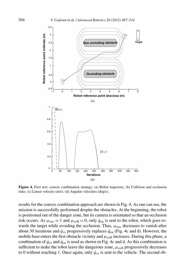
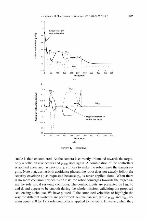
(a)

(b)

Figure 4. First test: convex combination strategy. (a) Robot trajectory. (b) Collision and occlusionrisks. (c) Linear velocity (m/s). (d) Angular velocities (deg/s).

results for the convex combination approach are shown in Fig. 4. As one can see, themission is successfully performed despite the obstacles. At the beginning, the robotis positioned out of the danger zone, but its camera is orientated so that an occlusionrisk occurs. As μocc = 1 and μcoll = 0, only qoa is sent to the robot, which goes to-wards the target while avoiding the occlusion. Thus, μocc decreases to vanish afterabout 30 iterations and qvs progressively replaces qoa (Fig. 4c and d). However, themobile base enters the first obstacle vicinity and μcoll increases. During this phase, acombination of qvs and qca is used as shown in Fig. 4c and d. As this combination issufficient to make the robot leave the dangerous zone, μcoll progressively decreasesto 0 without reaching 1. Once again, only qvs is sent to the vehicle. The second ob-

V. Cadenat et al. / Advanced Robotics 26 (2012) 487–514 505

(c)

(d)

Figure 4. (Continued.)

stacle is then encountered. As the camera is correctly orientated towards the target,only a collision risk occurs and μcoll rises again. A combination of the controllersis applied anew and, as previously, suffices to make the robot leave the danger re-gion. Note that, during both avoidance phases, the robot does not exactly follow thesecurity envelope ξ0 as requested because qca is never applied alone. When thereis no more collision nor occlusion risk, the robot converges towards the target us-ing the sole visual servoing controller. The control inputs are presented on Fig. 4cand d, and appear to be smooth during the whole mission, validating the proposedsequencing technique. We have plotted all the computed velocities to highlight theway the different switches are performed. As one can see, while μocc and μcoll re-main equal to 0 (or 1), a sole controller is applied to the robot. However, when they

506 V. Cadenat et al. / Advanced Robotics 26 (2012) 487–514

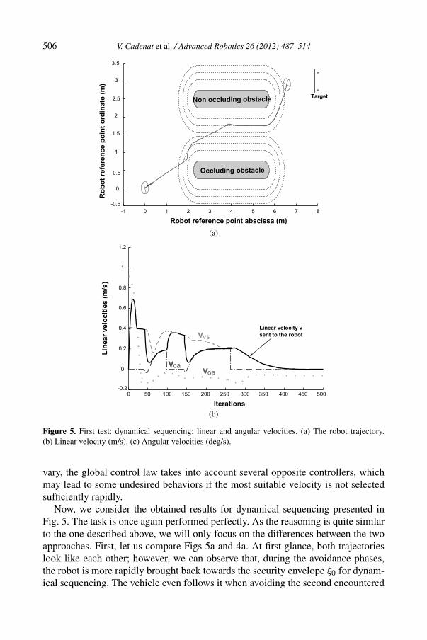
(a)

(b)

Figure 5. First test: dynamical sequencing: linear and angular velocities. (a) The robot trajectory.(b) Linear velocity (m/s). (c) Angular velocities (deg/s).

vary, the global control law takes into account several opposite controllers, whichmay lead to some undesired behaviors if the most suitable velocity is not selectedsufficiently rapidly.

Now, we consider the obtained results for dynamical sequencing presented inFig. 5. The task is once again performed perfectly. As the reasoning is quite similarto the one described above, we will only focus on the differences between the twoapproaches. First, let us compare Figs 5a and 4a. At first glance, both trajectorieslook like each other; however, we can observe that, during the avoidance phases,the robot is more rapidly brought back towards the security envelope ξ0 for dynam-ical sequencing. The vehicle even follows it when avoiding the second encountered

V. Cadenat et al. / Advanced Robotics 26 (2012) 487–514 507

(c)

Figure 5. (Continued.)

obstacle (the result is slightly different for the first obstacle, because the leavingcondition occurs before the robot has been settled on ξ0). This result is rather logi-cal. Indeed, as only the most relevant controller (and not a combination of oppositeones) is applied to the robot, the avoidance motion quality is significantly improved.The same reasoning holds when treating the occlusions. This particular character-istic is the main advantage of dynamical sequencing over convex combination. Letus now analyze the control input evolutions shown in Fig. 5b and c. As one can see,they remain smooth, which validates the proposed sequencing approach. Further-more, as mentioned before, we can observe that only the most suitable controller(and not several ones) is rapidly applied to the vehicle, limiting undesired behav-iors. Note that the transient time duration of a switch is fixed by the sole parameterτxx , making the implementation easier.

Now, we consider the second simulation test. Here, we clearly demonstrate thelimitations of convex combination approaches with respect to dynamical sequenc-ing. The results are presented in Fig. 6. Figure 6a shows that, for convex combina-tion, the robot has to perform maneuvers to avoid both collisions and occlusions,which occur in the first obstacle vicinity. Indeed, during this phase, as μcoll neverreaches 1 (Fig. 6c), three opposite controllers simultaneously act on the vehicle,making it go towards the obstacle and then backward. In fact, the robot is close toa local minimum. Fortunately, the maneuvers suffice to make the robot leave thiszone and the task can be finally performed. On the contrary, this problem does notoccur when using dynamical sequencing as shown by Fig. 6b. Indeed, as the mostrelevant controller is always applied, there is no risk of local minimum and ma-neuvers are no longer required. Once again, we observe that the robot accuratelyfollows the security envelope, which demonstrates that the quality of the avoidancemotion is improved. The mission can then be performed more efficiently thanks tothis last approach.

508 V. Cadenat et al. / Advanced Robotics 26 (2012) 487–514

(a)

(b)

Figure 6. Second test: results for dynamical sequencing and convex combination. (a) Convex combi-nation. (b) Dynamical sequencing. (c) Risks of collision and occlusion (convex combination).

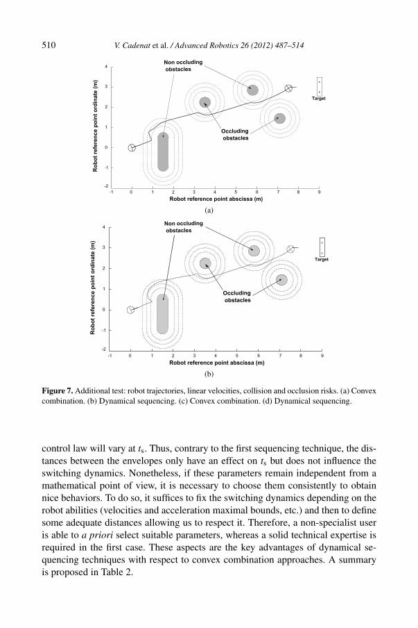
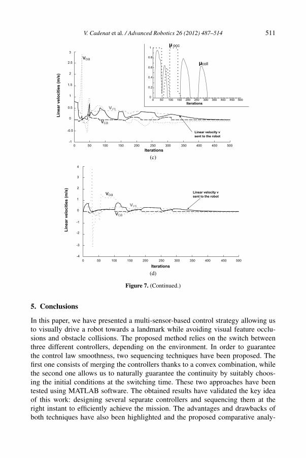
To demonstrate the efficiency of the proposed sequencing techniques, we presentone additional result where the environment is highly cluttered. As one can seefrom Fig. 7, the task is correctly performed with both approaches, despite severaloccluding and non-occluding obstacles. We do not detail the reasoning as it is quitesimilar to the previous cases.

4.2. Discussion

Now, we discuss the advantages and drawbacks of two sequencing techniques fromboth theoretical and practical points of view. The convex combination approach re-lies on a simple reasoning and allows us to independently design the three basiccontrollers using any convenient dynamics. Applications can then be rapidly car-ried out. This characteristic is its main advantage. However, it suffers from three

V. Cadenat et al. / Advanced Robotics 26 (2012) 487–514 509

(c)

Figure 6. (Continued.)

main drawbacks. (i) It is usually difficult to guarantee the task feasability becauseof local minima that may occur when different opposite controllers act on the robotat the same time (see Remark 3). (ii) The sequencing quality depends on numerousparameters (three control gains, three flags, two switching functions, six distances)that are strongly coupled: the three flags and the two switching functions dependon the six distances that have been defined to handle occlusions (D−, D0, D+) andcollisions (d−, d0, d+). (iii) All of them influence both the switching time and theway the control law will vary when switching. Thus, it is very difficult to a prioriset these parameters and evaluate how the control will behave when modifying one(or several) of them. Finally, simulations have shown that their values are closelyrelated to the task to be realized and to the environment (obstacles and goal loca-tions, robot initial configuration, etc.). Some technical expertise is then required toimplement the strategy.

Dynamical sequencing relies on a more complex mathematical theory than con-vex combination. However, this approach presents several strong advantages withrespect to the previous one. (i) It allows us to naturally guarantee the control lawsmoothness at the switching time. The continuity is only ensured at the first-order,which requires a careful choice of the gains λxx and τxx to avoid some saturationproblems at the acceleration level. (ii) The implementation is significantly simpli-fied for the following reasons. First of all, the proposed control strategy relies onthe definition of simple flags allowing us to detect the events that influence the taskexecution. If they are properly defined, only the most suitable controller (and nota combination of opposite control laws as previously) is applied to the robot. Theproblem of local minima is then noticeably reduced. Furthermore, few parameters(two gains and four flags depending on three distances) are involved in the controlstrategy. These parameters are mathematically discoupled; indeed, the four flagsdefine the time ts when the control has to switch and the two gains the way the

510 V. Cadenat et al. / Advanced Robotics 26 (2012) 487–514

(a)

(b)

Figure 7. Additional test: robot trajectories, linear velocities, collision and occlusion risks. (a) Convexcombination. (b) Dynamical sequencing. (c) Convex combination. (d) Dynamical sequencing.

control law will vary at ts. Thus, contrary to the first sequencing technique, the dis-tances between the envelopes only have an effect on ts but does not influence theswitching dynamics. Nonetheless, if these parameters remain independent from amathematical point of view, it is necessary to choose them consistently to obtainnice behaviors. To do so, it suffices to fix the switching dynamics depending on therobot abilities (velocities and acceleration maximal bounds, etc.) and then to definesome adequate distances allowing us to respect it. Therefore, a non-specialist useris able to a priori select suitable parameters, whereas a solid technical expertise isrequired in the first case. These aspects are the key advantages of dynamical se-quencing techniques with respect to convex combination approaches. A summaryis proposed in Table 2.

V. Cadenat et al. / Advanced Robotics 26 (2012) 487–514 511

(c)

(d)

Figure 7. (Continued.)

5. Conclusions

In this paper, we have presented a multi-sensor-based control strategy allowing usto visually drive a robot towards a landmark while avoiding visual feature occlu-sions and obstacle collisions. The proposed method relies on the switch betweenthree different controllers, depending on the environment. In order to guaranteethe control law smoothness, two sequencing techniques have been proposed. Thefirst one consists of merging the controllers thanks to a convex combination, whilethe second one allows us to naturally guarantee the continuity by suitably choos-ing the initial conditions at the switching time. These two approaches have beentested using MATLAB software. The obtained results have validated the key ideaof this work: designing several separate controllers and sequencing them at theright instant to efficiently achieve the mission. The advantages and drawbacks ofboth techniques have also been highlighted and the proposed comparative analy-

512 V. Cadenat et al. / Advanced Robotics 26 (2012) 487–514

Table 2.Comparative analysis summary

Sequencing Advantages Drawbackstechnique

Convex based on a simple reasoning high risk of local minimacombination acceleration constraints can be requires to choose numerous coupledapproach easily treated parameters that depend on the task, on

the robot and on the environmentrequires a solid technical expertise tofix the different parameters

Dynamical natural control law smoothness relies on a more complex mathematicalsequencing local minima problems are nearly theoryapproach suppressed sudden variations in the acceleration

requires few independent parameters may occurthat can be easily a priori chosen,on the basis of the robot abilitiesonce implemented, the technique canbe easily used by a non-specialist user

sis has clearly shown the interest of using dynamical sequencing instead of convexcombination to perform complex navigation tasks.

For future work, we first plan to experiment these approaches on our mobilerobot, as the obtained simulation results are quite satisfactory. From a more the-oretical point of view, different research axes may be considered. First, it wouldbe interesting to automatize the choice of parameters λxx , τxx and μxx to avoidundesirable accelerations values while keeping suitable decreasing speed and tran-sient time duration. We would also like to test other kinds of possible ‘switchingdynamics’ and compare them to those proposed in this work. Finally, using thesetechniques in other contexts to perform other kinds of missions or for different typesof robots appear to us as a great and interesting challenge.

References

1. F. Chaumette and S. Hutchinson, Visual servo control, part I: basic approaches, IEEE RoboticsAutomat. Mag. 13, 82–90 (2006).

2. E. Marchand and G. Hager, Dynamic sensor planning in visual servoing, in: Proc. IEEE Int. Conf.on Robotics and Automation, Leuven, pp. 1988–1993 (1998).

3. N. Mansard and F. Chaumette, A new redundancy formalism for avoidance in visual servoing,in: Proc. IEEE/RSJ Int. Conf. on Intelligent Robots and Systems, Edmonton, AB, pp. 1694–1700(2005).

4. Y. Mezouar and F. Chaumette, Avoiding self-occlusions and preserving visibility by path planningin the image, Robotics Autonomous Syst. 41, 77–87 (2002).

5. P. Corke and S. Hutchinson, A new partitioned approach to image-based visual servo control,IEEE Trans. Robotics Automat. 17, 507–515 (2001).

V. Cadenat et al. / Advanced Robotics 26 (2012) 487–514 513

6. V. Kyrki, D. Kragic and H. Christensen, New shortest-path approaches to visual servoing, in: Proc.IEEE/RSJ Int. Conf. on Intelligent Robots and Systems, Sendai, pp. 349–355 (2004).

7. S. Benhimane and E. Malis, Vision-based control with respect to planar and non-planar objectsusing a zooming camera, in: Proc. IEEE Int. Conf. on Autonomous Robots, Coimbra, pp. 991–996(2003).

8. A. Remazeilles, N. Mansard and F. Chaumette, Qualitative visual servoing: application to thevisibility constraint, in: Proc. IEEE/RSJ Int. Conf. on Intelligent Robots and Systems, Beijing,pp. 4297–4303 (2006).

9. V. Cadenat, P. Souères and M. Courdesses, Using system redundancy to perform a sensor-basednavigation task amidst obstacles, Int. J. Robotics Automat. 16, 61–73 (2001).

10. D. Folio and V. Cadenat, A controller to avoid both occlusions and obstacles during a vision-basednavigation task in a cluttered environment, in: Proc. Eur. Control Conf., Seville, pp. 3898–3903(2005).

11. R. Pissard-Gibollet and P. Rives, Applying visual servoing techniques to control a mobile hand–eye system, in: Proc. IEEE Int. Conf. on Robotics and Automation, Nagoya, pp. 166–171 (1995).

12. P. Souères and V. Cadenat, Dynamical sequence of multi-sensor based tasks for mobile robotsnavigation, in: Proc. IFAC Symp. on Robot Control, Wroclaw, pp. 423–428 (2003).

13. B. Gao, Contribution à la synthèse de commandes référencées vision 2D multi-critères, PhD Dis-sertation, University of Toulouse (2006).

14. N. Mansard and F. Chaumette, Task sequencing for sensor-based control, IEEE Trans. Robotics23, 60–72 (2007).

15. B. Espiau, F. Chaumette and P. Rives, A new approach to visual servoing in robotics, IEEE Trans.Robotics Automat. 8, 313–326 (1992).

16. F. Chaumette, Image moments: a general and useful set of features for visual servoing, IEEETrans. Robotics Automat. 20, 713–723 (2004).

17. C. Samson, M. L. Borgne and B. Espiau, Robot Control: The Task Function Approach. OxfordScience, Oxford (1991).

18. N. Garcia-Aracil, J. A. Poveda, J. S. Navarro, C. P. Vidal and R. S. Pazmino, Visual controlof robots with changes of visibility in image features, IEEE Trans. Robotics Automat. 4, 27–33(2006).

19. V. Cadenat, P. Souères and T. Hamel, A reactive path-following controller to guarantee obstacleavoidance during the transient phase, Int. J. Robotics Automat. 21, 256–265 (2006).

20. C. Samson, Path following and time-varying feedback stabilization of a wheeled mobile robot,in: Proc. Int. Conf. on Control Automation, Robotics and Vision, Singapore, pp. RO-13.1.1–RO-13.1.5 (1992).

21. P. Souères, T. Hamel and V. Cadenat, A path following controller for wheeled robots which al-lows to avoid obstacles during the transition phase, in: Proc. IEEE Int. Conf. on Robotics andAutomation, Leuven, pp. 1269–1274 (1998).

514 V. Cadenat et al. / Advanced Robotics 26 (2012) 487–514

About the Authors

Viviane Cadenat obtained her PhD, in 1999, from Paul Sabatier University,Toulouse, France. She was hired as an Associate Professor at Paul Sabatier Uni-versity, in 2000. She is currently teaching robotics and automatic control theory atboth the Bachelor and the Master levels. She is also Member of the RAP (Robotics,Action and Perception) group from the Laboratory for Analysis and Architec-ture of Systems (LAAS) and is still interested in the navigation of a mobile robotamidst obstacles using vision-based control.

David Folio received his PhD degree in Control Systems, in 2007, in the RoboticAction and Perception (RAP) group of the Laboratory for Analysis and Archi-tecture of Systems (LAAS), Toulouse, France. Between 2007 and 2008, he wasa Postdoctorate Fellow in the Lagadic team of the IRISA Laboratory, Rennes,France. He has worked on the design of sensor-based control strategies able totolerate data loss. Since 2008, he has been an Assistant Professor at the InstitutPRISME, Ecole Nationale Supérieure d’Ingénieurs de Bourges (ENSI Bourges),Bourges, France. He is now working on the design and modeling of navigation

control strategies for micro and nanorobotics systems.

Adrien Durand Petiteville is PhD student in the Robotic Action and Percep-tion (RAP) Group of the Laboratory for Analysis and Architecture of Systems(LAAS), Toulouse, France. He is working on sensor-based navigation in clutteredenvironments.