C. Delire Æ S. Levis Æ G. Bonan Æ J.A. Foley Æ M. Coe

S. Vavrus

Comparison of the climate simulated by the CCM3 coupledto two different land-surface models

Received: 21 March 2001 /Accepted: 29 March 2002 / Published online: 22 June 2002� Springer-Verlag 2002

Abstract We present results from a coupled atmo-sphere–biosphere model CCM3/IBIS (the CommunityClimate Model coupled to the Integrated BIosphereSimulator), which is designed to study the dynamic in-teractions between climate and vegetation and the globalcarbon cycle. We analyze the climate simulated byCCM3/IBIS with fixed vegetation conditions and wecompare it to the climate simulated by the standardCCM3, which includes the LSM (land surface model)land-surface package. Important differences between thetwo models include simple parametrizations of lakes,wetlands and crops in CCM3/LSM not taken into ac-count in CCM3/IBIS. CCM3/IBIS and CCM3/LSMshare common biases (compared to observations) in thetemperature field in boreal winter and in the precipita-tion field annually, making the atmospheric model themost probable cause of those biases. The models differ inthe temperature field and surface energy balance in theSahara annually and in the mid-to high latitudes fromspring through fall. CCM3/IBIS simulates global annualair temperatures that are on average 1.7 �C higher thanCCM3/LSM and 0.5 �C higher than the observed cli-matology. Differences in albedo and/or snow paramet-rization explain most of the Sahara and high-latitudetemperature disagreement. Our sensitivity study with

CCM3/LSM shows that the presence of lakes and wet-lands in CCM3/LSM can account for about half of thedifference in temperature in summer over the lake andwetland regions of the mid-latitudes. A second sensi-tivity study shows that higher surface roughness lengthin CCM3/IBIS can also explain part of the difference insummer surface temperature in the mid-latitudes. Sur-face roughness length affects the surface temperaturethrough a feedback mechanism linking surface windspeed, planetary boundary layer height, low levelcloudiness and radiation.

1 Introduction

The land surface exchanges water, energy, momentumand also CO2 with the atmosphere, therefore playing animportant role in the climate system. Changes in theland surface properties, due to human activity orchanging climate, affect those exchange processes andare likely to affect the climate itself. Given the potentialimportance of land surface processes in the climatesystem, efforts have been made to develop process-basedbiophysical models of land–atmosphere exchange pro-cesses and to couple them to general circulation models.There now exist a large number of land surface modelsthat differ greatly in the choice of processes included andin the degree of complexity used to represent each pro-cess.The vast majority of the land surface models coupled

to general circulation models (GCMs) simulate the ex-change of water, energy and momentum at the surfacegiven a prescribed geographical distribution of the veg-etation and soils. They are designed to simulate the cli-mate at a time scale of a few years to a few decades whenvegetation changes can be neglected. Some models alsocalculate the CO2 exchange using a parametrization ofthe soil respiration flux (i.e. LSM, Bonan, 1995a, andSiB2, Sellers et al. 1996).

Climate Dynamics (2002) 19: 657–669DOI 10.1007/s00382-002-0255-7

C. Delire (&) Æ J.A. Foley Æ M. CoeCenter for Sustainability and the Global Environment (SAGE),Gaylord Nelson Institute for Environmental Studies,University of Wisconsin, 1710 University Avenue,Madison, WI 53726, USAE-mail: cldelire@facstaff.wisc.edu

S. Levis Æ G. BonanNational Center for Atmospheric Research,PO Box 3000 Boulder, CO 80307-3000, USA

S. VavrusCenter for Climatic Research,Institute for Environmental Studies,University of Wisconsin, 1225 W Dayton St.,Madison, WI 53706-1695, USA

A small number of land surface models designed tobe coupled to GCMs also represent the dynamics of thevegetation and the carbon cycling in vegetation and soils(i.e. TRIFFID, (Cox et al. 2000) and IBIS (Foley et al.1996; Kucharik et al. 2000)). IBIS (Integrated BIosphereSimulator) was built to simulate land surface processes,terrestrial carbon and nutrient cycling, and vegetationdynamics in a coherent and mechanistic way. IBIS hasthe capability to simulate short and long time scaleprocesses, therefore providing an excellent tool that canbe used inside a coupled atmosphere–ocean GCM. IBISwas first coupled to the GENESIS atmospheric GCM ofThompson and Pollard (Thompson and Pollard, 1995a,b) and used to study vegetation feedbacks in differentclimatic regimes (Foley et al. 1998, 2000; Levis et al.1999a, b, 2000).Here we coupled IBIS to the Community Climate

Model CCM3 (Kiehl et al. 1998) in order to provide atool to study climate-vegetation dynamics and the globalcarbon cycle, which LSM, the standard land surfacemodel of the CCM3, does not do. Our first goal is tounderstand and document how the use of IBIS in theCCM3 affects the simulated climate. Therefore, wecompare the climate simulated by CCM3 coupled withIBIS, to the climate simulated by CCM3 coupled withLSM. Both simulated climates are also compared toobservations. We chose to operate IBIS with prescribedvegetation as a regular land surface model to ease thecomparison with LSM.Our second goal is a by-product of this comparison:

by using two different land surface models coupled tothe same GCM, we can investigate whether known bi-ases of the GCM can be attributed to the land surfacemodels or if they are inherent to the atmospheric part ofthe model.Analyzing the results of coupled models is a difficult

task because of the feedback mechanisms taking place.There have been three major efforts aimed at comparingand evaluating land surface models and GCMs. ThePILPS (Project for Intercomparison of Land-surfaceParametrization Schemes) activity has compared thesimulation of roughly 20 land surface models separatelyfrom their host GCMs (off-line experiments) usingidentical observed or idealized atmospheric forcing andidentical surface characteristics. These off-line experi-ments showed large discrepancies in the partitioning ofavailable energy into latent and sensible heat and thepartitioning of precipitation into evapotranspiration andrunoff or drainage (Qu and Henderson-Sellers 1998).The Atmospheric Model Intercomparison Project(AMIP) (Gates 1992; Gates et al. 1999) and the Paleo-climate Modelling Intercomparison Project (PMIP)(Braconnot 2000) aimed at comparing the climate sim-ulated by 20 to 30 different AGCMs for present and pastconditions. The models were run at different resolutionswith different land surface boundary conditions anddifferent parametrizations of, among others, landsurface processes. Diagnosing if the land surface is theorigin of the differences among the results of the models

is a particularly difficult exercise when the atmosphericmodels are different. One conclusion that could bedrawn from this exercise is that the land surface is not areliable indicator of a model’s ability to simulate pre-cipitation (Boyle 1998). Here, by comparing two differ-ent land surface models in the same GCM, we can beginto see whether known biases of the GCM can beattributed to the land surface models or if they areinherent to the atmospheric part of the model.

2 IBIS-2 and LSM: model descriptions

In this study, we use an updated version of the Integrated Bio-sphere Simulator (IBIS) of Foley et al. (1996) and Kucharik et al.(2000). IBIS (version 2) is a comprehensive model of terrestrialbiospheric processes, and includes land-surface physics, canopyphysiology, plant phenology, vegetation dynamics and competi-tion, and carbon cycling. The IBIS land surface module simulatesthe energy, water, carbon, and momentum balance of the soil-vegetation-atmosphere system on a short time step consistent withGCMs (�20 to 60 min). The land surface module borrows much ofits basic structure from the LSX land surface package.(Thompsonand Pollard 1995a, b) The module includes two vegetation layers(i.e., ‘‘trees’’ and ‘‘grasses and shrubs’’) and six soil layers to sim-ulate soil temperature, soil water, and soil ice content over a totaldepth of 4 m. Physiologically based formulations of C3 and C4photosynthesis, (Farquhar et al. 1980) stomatal conductance(Collatz et al. 1991, 1992) and respiration (Amthor 1984) are usedto simulate canopy gas exchange processes. This approach providesa mechanistic link between the exchange of energy, water, and CO2between vegetation canopies and the atmosphere. Budburst andsenescence depend on climatic factors following the empirical al-gorithm presented by Botta (2000). The annual carbon balanceallows the vegetation dynamics sub-model to predict the maximumleaf area index and biomass for 12 plant functional types, whichcompete for light and water. The model can also operate with afixed vegetation distribution, which is used in this study.LSM (Bonan 1996) does not differ much from the land surface

module of IBIS and, conceptually, fulfills the same purpose bysimulating the exchange of energy, water, carbon, and momentumat the land–atmosphere interface. Vegetated surfaces include up tothree plant types per grid cell distributed in patches. Lakes andwetlands (Cogley 1991) when present, form up to two additionalpatches per grid cell. The model operates independently within eachsubgrid patch, although the same atmospheric forcing applies tothe entire grid cell. A set of land cover types (Olson et al. 1983),combined with corresponding plant types, and their monthly leafareas (Dorman and Sellers 1989) describe the landscape. Thismodel has six soil layers to a total depth of 6.3 m. As with IBIS,photosynthesis and stomatal conductance are based on Farquharet al. (1980) and Collatz et al. (1991, 1992) respectively. Respirationfollows Bonan (1995a) and Jones (1992).The main differences between IBIS and LSM are:

1. IBIS is able to describe vegetation dynamics and carbon cyclingin the soil and vegetation, whereas LSM cannot. In this studyhowever, IBIS is used with a prescribed vegetation map so thatthe vegetation dynamics and carbon cycling in soils modules arenot turned on.

2. LSM includes a parametrization of inland water bodies (lakesand wetlands) (Bonan 1995b) but IBIS does not.

3. LSM includes a simple representation of crops while IBIS rep-resents only natural vegetation types.

4. Budburst and senescence in IBIS depend on the climate. In thecurrent version of LSM, the phenology depends solely on thecalendar date.

5. Each grid cell in IBIS has a vegetation cover made up of acombination of up to 12 plant functional types. When IBIS isused with fixed vegetation, as in this study, this combination is

658 Delire et al.: Comparison of the climate simulated by the CCM3 coupled to two different land-surface models

fixed in each grid cell and acts as a single homogeneous vege-tation type. In LSM, each grid cell contains up to three patches(or tiles), each with a different single vegetation type, plus up totwo more patches with lake or wetland.

6. IBIS describes two canopies, one for grasses and shrubs, and theother for trees. LSM describes one canopy, either trees or grass.

7. With IBIS, physical parameters describing the vegetation, suchas canopy height or roughness length, depend on the evolutionof LAI and the carbon balance. In LSM they are fixed anddepend solely on the vegetation type.

3 Simulations and data set used

We performed a total of four 20-year simulations with the NCARCCM3 at a resolution of T31 (�3.75� · 3.75�): two main simula-tions and two sensitivity studies. We used LSM as the land-surfacemodel for the first main control simulation and IBIS replacingLSM for the second. We then performed two sensitivity studieswith CCM3/LSM. Fixed climatological sea surface temperatures(SSTs) were used for all the runs. We chose the T31 resolutionbecause it is the resolution that will most likely be used in globalcarbon cycle studies due to computing time constraints. The last 15years of each run are used for averaging.Soil texture is prescribed in IBIS from the IGBP-DIS global

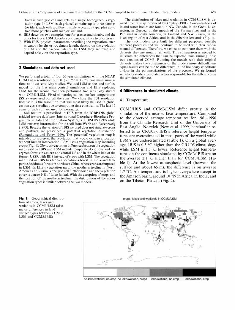
gridded texture database (International Geosphere–Biosphere Pro-gramme – Data and Information System), (IGBP-DIS 1999) whileLSM retrieves information for the soil from Webb and Rosenzweig(1993). Because the version of IBIS we used does not simulate cropsand pastures, we prescribed a potential vegetation distribution(Ramankutty and Foley 1999). The ‘potential’ vegetation map isintended to represent the vegetation that would exist in a locationwithout human intervention. LSM uses a vegetation map includingcrops (Fig. 1).Obvious vegetation differences between the vegetationmaps used in IBIS and LSM include temperate deciduous and ev-ergreen forests in eastern and central US and in the wheat belt of theformer USSR with IBIS instead of crops with LSM. The vegetationmap used in IBIS has tropical deciduous forest in India and tem-perate deciduous forests in northeastChina,where crops are imposedin LSM. In IBIS’s vegetation map, the northern treeline in NorthAmerica and Russia is one grid cell further north and the vegetationcover is denser NE of Lake Baikal. With the exception of crops andthe location of the northern treeline, the distribution of the majorvegetation types is similar between the two models.

The distribution of lakes and wetlands in CCM3/LSM is de-rived from a map produced by Cogley (1991). Concentrations ofinland water bodies are found in NW Canada, in the Great Lakesregion, in Quebec, at the mouth of the Parana river and in thePantanal in South America, in Finland and NW Russia, in thelakes region of east Africa, and in the Siberian lowlands (Fig. 1).The two models were built for different purposes, describe

different processes and will continue to be used with their funda-mental differences. Therefore, we chose to compare them with thedatasets they are usually run with. This comparison is needed toillustrate the differences that can be expected from running thosetwo versions of CCM3. Running the models with their originaldatasets makes the comparison of the models more difficult: un-equal results can be due to differences in the boundary conditionsand/or in the parametrizations of the processes. We performedsensitivity studies to isolate factors responsible for the differences inthe simulated climate.

4 Differences in simulated climate

4.1 Temperature

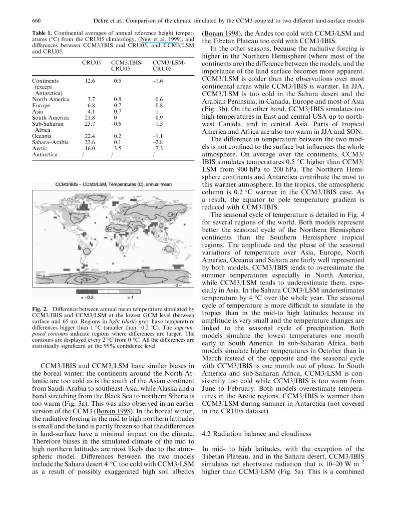
CCM3/IBIS and CCM3/LSM differ greatly in thesimulation of the near-surface temperature. Comparedto the observed average temperatures for 1961–1990from the Climate Research Unit of the University ofEast Anglia, Norwich (New et al. 1999, hereinafter re-ferred to as CRU05), IBIS’s reference height tempera-tures are overestimated in most parts of the world whileLSM’s are underestimated (Table 1). On a global aver-age, IBIS is 0.5 �C higher than the CRU05 climatologywhile LSM is 1.5 �C lower. Reference height tempera-tures on the continents simulated by CCM3/IBIS are onthe average 2.1 �C higher than for CCM3/LSM (Ta-ble 1). At the lowest atmospheric level (between thesurface and about 65 m), the difference is on average1.7 �C. Air temperature is higher everywhere except inthe Amazon basin, around 10 �N in Africa, in India, andon the Tibetan Plateau (Fig. 2).

Fig. 1. Geographical distribu-tion of crops, lakes andwetlands in CCM3/LSM (alsomajor differences in landsurface types between CCM3/LSM and CCM3/IBIS)

Delire et al.: Comparison of the climate simulated by the CCM3 coupled to two different land-surface models 659

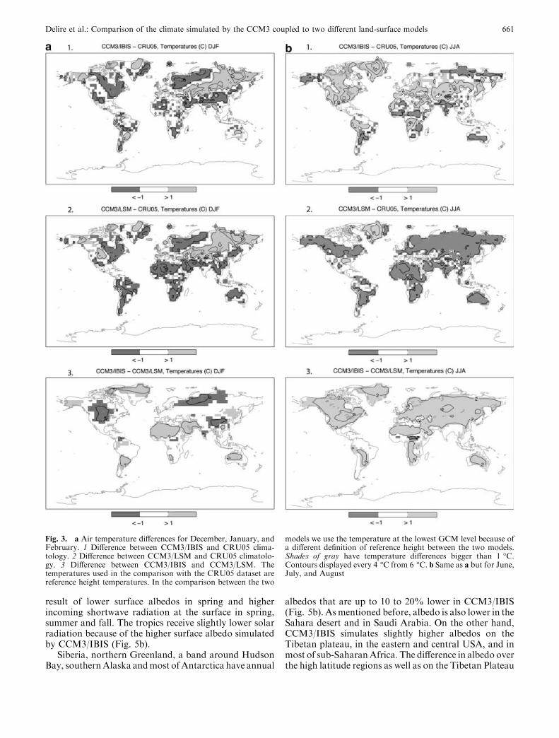
CCM3/IBIS and CCM3/LSM have similar biases inthe boreal winter: the continents around the North At-lantic are too cold as is the south of the Asian continentfrom Saudi-Arabia to southeast Asia, while Alaska and aband stretching from the Black Sea to northern Siberia istoo warm (Fig. 3a). This was also observed in an earlierversion of the CCM3 (Bonan 1998). In the boreal winter,the radiative forcing in the mid to high northern latitudesis small and the land is partly frozen so that the differencesin land-surface have a minimal impact on the climate.Therefore biases in the simulated climate of the mid tohigh northern latitudes are most likely due to the atmo-spheric model. Differences between the two modelsinclude the Sahara desert 4 �C too cold with CCM3/LSMas a result of possibly exaggerated high soil albedos

(Bonan 1998), the Andes too cold with CCM3/LSM andthe Tibetan Plateau too cold with CCM3/IBIS.In the other seasons, because the radiative forcing is

higher in the Northern Hemisphere (where most of thecontinents are) the difference between themodels, and theimportance of the land surface becomes more apparent.CCM3/LSM is colder than the observations over mostcontinental areas while CCM3/IBIS is warmer. In JJA,CCM3/LSM is too cold in the Sahara desert and theArabian Peninsula, in Canada, Europe and most of Asia(Fig. 3b). On the other hand, CCM3/IBIS simulates toohigh temperatures in East and central USA up to north-west Canada, and in central Asia. Parts of tropicalAmerica and Africa are also too warm in JJA and SON.The difference in temperature between the two mod-

els is not confined to the surface but influences the wholeatmosphere. On average over the continents, CCM3/IBIS simulates temperatures 0.5 �C higher than CCM3/LSM from 900 hPa to 200 hPa. The Northern Hemi-sphere continents and Antarctica contribute the most tothis warmer atmosphere. In the tropics, the atmosphericcolumn is 0.2 �C warmer in the CCM3/IBIS case. Asa result, the equator to pole temperature gradient isreduced with CCM3/IBIS.The seasonal cycle of temperature is detailed in Fig. 4

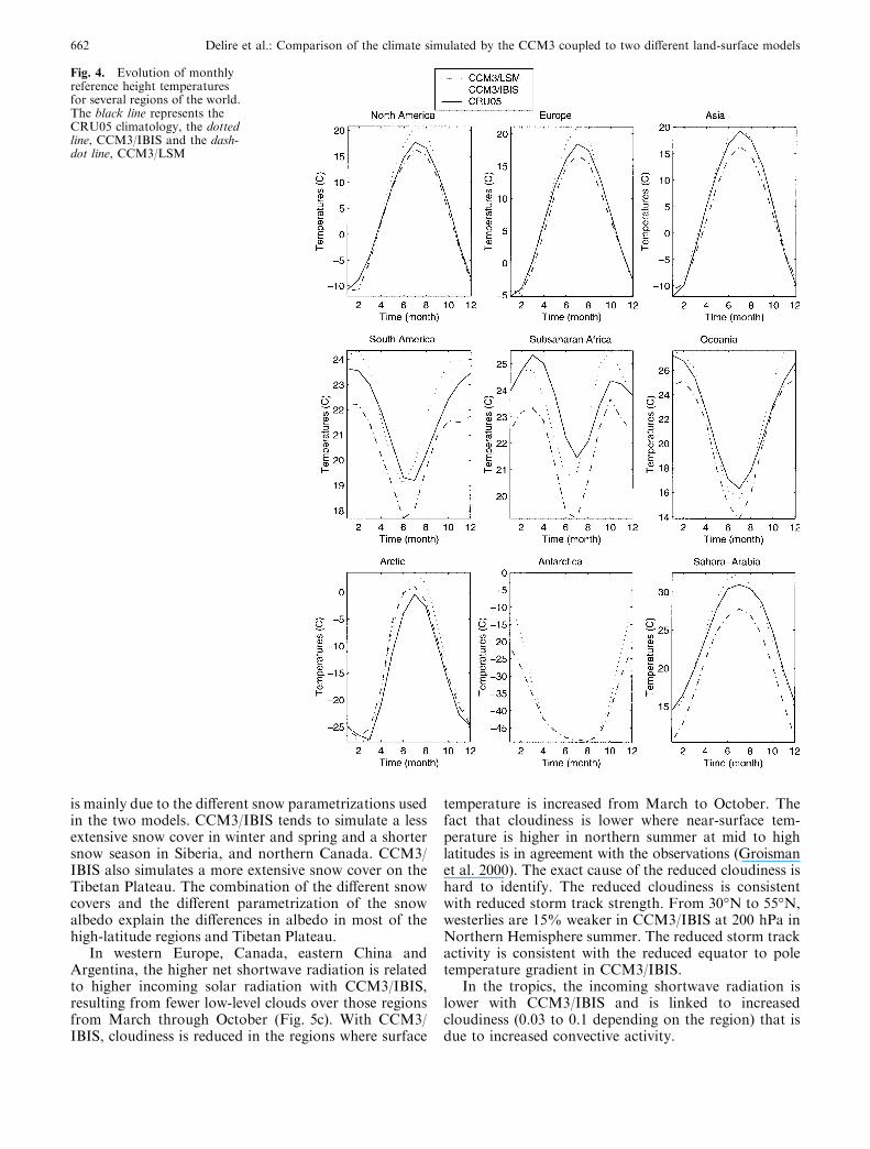
for several regions of the world. Both models representbetter the seasonal cycle of the Northern Hemispherecontinents than the Southern Hemisphere tropicalregions. The amplitude and the phase of the seasonalvariations of temperature over Asia, Europe, NorthAmerica, Oceania and Sahara are fairly well representedby both models. CCM3/IBIS tends to overestimate thesummer temperatures especially in North America,while CCM3/LSM tends to underestimate them, espe-cially in Asia. In the Sahara CCM3/LSM underestimatestemperature by 4 �C over the whole year. The seasonalcycle of temperature is more difficult to simulate in thetropics than in the mid-to high latitudes because itsamplitude is very small and the temperature changes arelinked to the seasonal cycle of precipitation. Bothmodels simulate the lowest temperatures one monthearly in South America. In sub-Saharan Africa, bothmodels simulate higher temperatures in October than inMarch instead of the opposite and the seasonal cyclewith CCM3/IBIS is one month out of phase. In SouthAmerica and sub-Saharan Africa, CCM3/LSM is con-sistently too cold while CCM3/IBIS is too warm fromJune to February. Both models overestimate tempera-tures in the Arctic regions. CCM3/IBIS is warmer thanCCM3/LSM during summer in Antarctica (not coveredin the CRU05 dataset).

4.2 Radiation balance and cloudiness

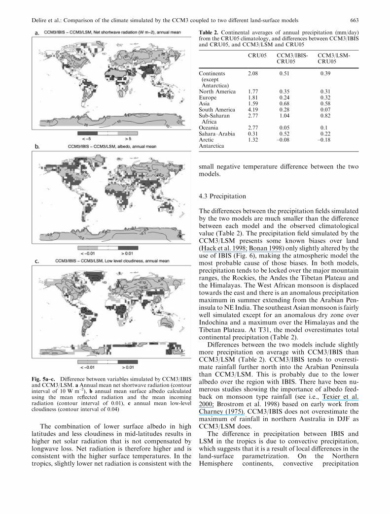
In mid- to high latitudes, with the exception of theTibetan Plateau, and in the Sahara desert, CCM3/IBISsimulates net shortwave radiation that is 10–20 W m–2

higher than CCM3/LSM (Fig. 5a). This is a combined

Table 1. Continental averages of annual reference height temper-atures (�C) from the CRU05 climatology, (New et al. 1999), anddifferences between CCM3/IBIS and CRU05, and CCM3/LSMand CRU05

CRU05 CCM3/IBIS-CRU05

CCM3/LSM-CRU05

Continents(exceptAntarctica)

12.6 0.5 –1.6

North America 3.7 0.8 –0.6Europe 6.8 0.7 –0.8Asia 4.1 0.7 –1South America 21.8 0 –0.9Sub-SaharanAfrica

23.7 –0.6 –1.3

Oceania 22.4 0.2 –1.1Sahara–Arabia 23.6 0.1 –2.8Arctic –16.0 3.5 2.3Antarctica / / /

Fig. 2. Difference between annual mean temperature simulated byCCM3/IBIS and CCM3/LSM at the lowest GCM level (betweensurface and 65 m). Regions in light (dark) gray have temperaturedifferences bigger than 1 �C (smaller than –0.2 �C). The superim-posed contours indicate regions where differences are larger. Thecontours are displayed every 2 �C from 0 �C. All the differences arestatistically significant at the 99% confidence level

660 Delire et al.: Comparison of the climate simulated by the CCM3 coupled to two different land-surface models

result of lower surface albedos in spring and higherincoming shortwave radiation at the surface in spring,summer and fall. The tropics receive slightly lower solarradiation because of the higher surface albedo simulatedby CCM3/IBIS (Fig. 5b).Siberia, northern Greenland, a band around Hudson

Bay, southernAlaska andmost ofAntarctica have annual

albedos that are up to 10 to 20% lower in CCM3/IBIS(Fig. 5b). Asmentioned before, albedo is also lower in theSahara desert and in Saudi Arabia. On the other hand,CCM3/IBIS simulates slightly higher albedos on theTibetan plateau, in the eastern and central USA, and inmost of sub-SaharanAfrica. The difference in albedo overthe high latitude regions as well as on the Tibetan Plateau

Fig. 3. a Air temperature differences for December, January, andFebruary. 1 Difference between CCM3/IBIS and CRU05 clima-tology. 2 Difference between CCM3/LSM and CRU05 climatolo-gy. 3 Difference between CCM3/IBIS and CCM3/LSM. Thetemperatures used in the comparison with the CRU05 dataset arereference height temperatures. In the comparison between the two

models we use the temperature at the lowest GCM level because ofa different definition of reference height between the two models.Shades of gray have temperature differences bigger than 1 �C.Contours displayed every 4 �C from 6 �C. b Same as a but for June,July, and August

Delire et al.: Comparison of the climate simulated by the CCM3 coupled to two different land-surface models 661

is mainly due to the different snow parametrizations usedin the two models. CCM3/IBIS tends to simulate a lessextensive snow cover in winter and spring and a shortersnow season in Siberia, and northern Canada. CCM3/IBIS also simulates a more extensive snow cover on theTibetan Plateau. The combination of the different snowcovers and the different parametrization of the snowalbedo explain the differences in albedo in most of thehigh-latitude regions and Tibetan Plateau.In western Europe, Canada, eastern China and

Argentina, the higher net shortwave radiation is relatedto higher incoming solar radiation with CCM3/IBIS,resulting from fewer low-level clouds over those regionsfrom March through October (Fig. 5c). With CCM3/IBIS, cloudiness is reduced in the regions where surface

temperature is increased from March to October. Thefact that cloudiness is lower where near-surface tem-perature is higher in northern summer at mid to highlatitudes is in agreement with the observations (Groismanet al. 2000). The exact cause of the reduced cloudiness ishard to identify. The reduced cloudiness is consistentwith reduced storm track strength. From 30�N to 55�N,westerlies are 15% weaker in CCM3/IBIS at 200 hPa inNorthern Hemisphere summer. The reduced storm trackactivity is consistent with the reduced equator to poletemperature gradient in CCM3/IBIS.In the tropics, the incoming shortwave radiation is

lower with CCM3/IBIS and is linked to increasedcloudiness (0.03 to 0.1 depending on the region) that isdue to increased convective activity.

Fig. 4. Evolution of monthlyreference height temperaturesfor several regions of the world.The black line represents theCRU05 climatology, the dottedline, CCM3/IBIS and the dash-dot line, CCM3/LSM

662 Delire et al.: Comparison of the climate simulated by the CCM3 coupled to two different land-surface models

The combination of lower surface albedo in highlatitudes and less cloudiness in mid-latitudes results inhigher net solar radiation that is not compensated bylongwave loss. Net radiation is therefore higher and isconsistent with the higher surface temperatures. In thetropics, slightly lower net radiation is consistent with the

small negative temperature difference between the twomodels.

4.3 Precipitation

The differences between the precipitation fields simulatedby the two models are much smaller than the differencebetween each model and the observed climatologicalvalue (Table 2). The precipitation field simulated by theCCM3/LSM presents some known biases over land(Hack et al. 1998; Bonan 1998) only slightly altered by theuse of IBIS (Fig. 6), making the atmospheric model themost probable cause of those biases. In both models,precipitation tends to be locked over the major mountainranges, the Rockies, the Andes the Tibetan Plateau andthe Himalayas. The West African monsoon is displacedtowards the east and there is an anomalous precipitationmaximum in summer extending from the Arabian Pen-insula toNE India. The southeastAsianmonsoon is fairlywell simulated except for an anomalous dry zone overIndochina and a maximum over the Himalayas and theTibetan Plateau. At T31, the model overestimates totalcontinental precipitation (Table 2).Differences between the two models include slightly

more precipitation on average with CCM3/IBIS thanCCM3/LSM (Table 2). CCM3/IBIS tends to overesti-mate rainfall further north into the Arabian Peninsulathan CCM3/LSM. This is probably due to the loweralbedo over the region with IBIS. There have been nu-merous studies showing the importance of albedo feed-back on monsoon type rainfall (see i.e., Texier et al.2000; Brostrom et al. 1998) based on early work fromCharney (1975). CCM3/IBIS does not overestimate themaximum of rainfall in northern Australia in DJF asCCM3/LSM does.The difference in precipitation between IBIS and

LSM in the tropics is due to convective precipitation,which suggests that it is a result of local differences in theland-surface parametrization. On the NorthernHemisphere continents, convective precipitation

Fig. 5a–c. Difference between variables simulated by CCM3/IBISand CCM3/LSM. a Annual mean net shortwave radiation (contourinterval of 10 W m–2), b annual mean surface albedo calculatedusing the mean reflected radiation and the mean incomingradiation (contour interval of 0.01), c annual mean low-levelcloudiness (contour interval of 0.04)

Table 2. Continental averages of annual precipitation (mm/day)from the CRU05 climatology, and differences between CCM3/IBISand CRU05, and CCM3/LSM and CRU05

CRU05 CCM3/IBIS-CRU05

CCM3/LSM-CRU05

Continents(exceptAntarctica)

2.08 0.51 0.39

North America 1.77 0.35 0.31Europe 1.81 0.24 0.32Asia 1.59 0.68 0.58South America 4.19 0.28 0.07Sub-SaharanAfrica

2.77 1.04 0.82

Oceania 2.77 0.05 0.1Sahara–Arabia 0.31 0.52 0.22Arctic 1.32 –0.08 –0.18Antarctica

Delire et al.: Comparison of the climate simulated by the CCM3 coupled to two different land-surface models 663

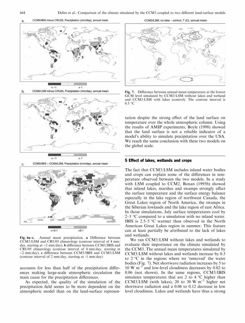
accounts for less than half of the precipitation differ-ences making large-scale atmospheric circulation themain cause for the precipitation differences.As expected, the quality of the simulation of the

precipitation field seems to be more dependent on theatmospheric model than on the land-surface represen-

tation despite the strong effect of the land surface ontemperature over the whole atmospheric column. Usingthe results of AMIP experiments, Boyle (1998) showedthat the land surface is not a reliable indicator of amodel’s ability to simulate precipitation over the USA.We reach the same conclusion with these two models onthe global scale.

5 Effect of lakes, wetlands and crops

The fact that CCM3/LSM includes inland water bodiesand crops can explain some of the differences in tem-perature observed between the two models. In a studywith LSM coupled to CCM2, Bonan (1995b) showedthat inland lakes, marshes and swamps strongly affectthe surface temperature and the surface energy balanceespecially in the lake region of northwest Canada, theGreat Lakes region of North America, the swamps inthe Siberian lowlands and the lake region of east Africa.In those simulations, July surface temperatures cool by2–3 �C compared to a simulation with no inland water.IBIS is 2.5–5 �C warmer than observed in the NorthAmerican Great Lakes region in summer. This featurecan at least partially be attributed to the lack of lakesand wetlands.We ran CCM3/LSM without lakes and wetlands to

evaluate their importance on the climate simulated bythe CCM3. The annual mean temperatures simulated byCCM3/LSM without lakes and wetlands increase by 0.5to 2 �C in the regions where we ‘removed’ the waterbodies (Fig. 7). Net shortwave radiation increases by 5 to10 W m–2 and low-level cloudiness decreases by 0.02 to0.06 (not shown). In the same regions, CCM3/IBISsimulates temperatures that are 2 to 4 �C higher thanCCM3/LSM (with lakes), 20 to 30 W m–2 higher netshortwave radiation and a 0.06 to 0.12 decrease in lowlevel cloudiness. Lakes and wetlands have thus a strong

Fig. 6a–c. Annual mean precipitation. a Difference betweenCCM3/LSM and CRU05 climatology (contour interval of 4 mm/day, starting at )2 mm/day), b difference between CCM3/IBIS andCRU05 climatology (contour interval of 4 mm/day, starting at)2 mm/day), c difference between CCM3/IBIS and CCM3/LSM(contour interval of 2 mm/day, starting at -1 mm/day)

Fig. 7. Difference between annual mean temperature at the lowestGCM level simulated by CCM3/LSM without lakes and wetlandand CCM3/LSM with lakes (control). The contour interval is0.5 �C

664 Delire et al.: Comparison of the climate simulated by the CCM3 coupled to two different land-surface models

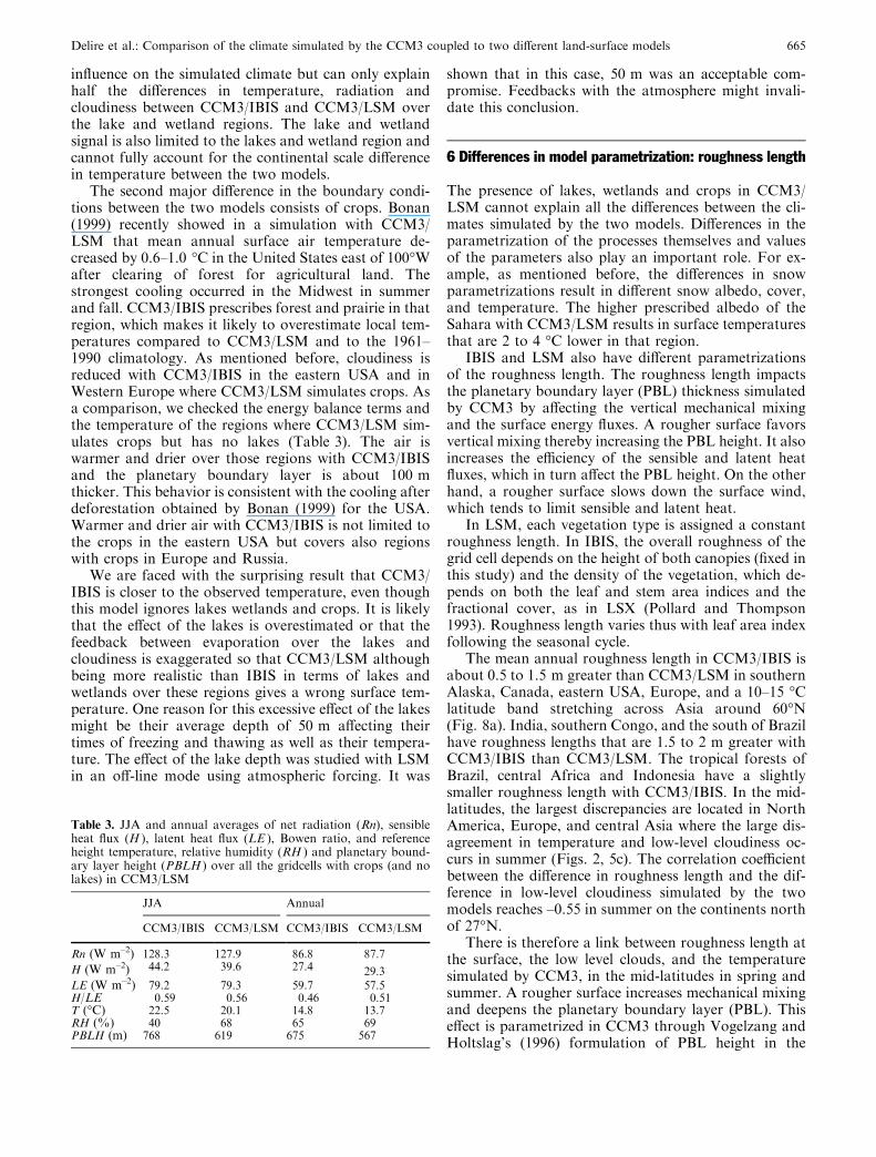
influence on the simulated climate but can only explainhalf the differences in temperature, radiation andcloudiness between CCM3/IBIS and CCM3/LSM overthe lake and wetland regions. The lake and wetlandsignal is also limited to the lakes and wetland region andcannot fully account for the continental scale differencein temperature between the two models.The second major difference in the boundary condi-

tions between the two models consists of crops. Bonan(1999) recently showed in a simulation with CCM3/LSM that mean annual surface air temperature de-creased by 0.6–1.0 �C in the United States east of 100�Wafter clearing of forest for agricultural land. Thestrongest cooling occurred in the Midwest in summerand fall. CCM3/IBIS prescribes forest and prairie in thatregion, which makes it likely to overestimate local tem-peratures compared to CCM3/LSM and to the 1961–1990 climatology. As mentioned before, cloudiness isreduced with CCM3/IBIS in the eastern USA and inWestern Europe where CCM3/LSM simulates crops. Asa comparison, we checked the energy balance terms andthe temperature of the regions where CCM3/LSM sim-ulates crops but has no lakes (Table 3). The air iswarmer and drier over those regions with CCM3/IBISand the planetary boundary layer is about 100 mthicker. This behavior is consistent with the cooling afterdeforestation obtained by Bonan (1999) for the USA.Warmer and drier air with CCM3/IBIS is not limited tothe crops in the eastern USA but covers also regionswith crops in Europe and Russia.We are faced with the surprising result that CCM3/

IBIS is closer to the observed temperature, even thoughthis model ignores lakes wetlands and crops. It is likelythat the effect of the lakes is overestimated or that thefeedback between evaporation over the lakes andcloudiness is exaggerated so that CCM3/LSM althoughbeing more realistic than IBIS in terms of lakes andwetlands over these regions gives a wrong surface tem-perature. One reason for this excessive effect of the lakesmight be their average depth of 50 m affecting theirtimes of freezing and thawing as well as their tempera-ture. The effect of the lake depth was studied with LSMin an off-line mode using atmospheric forcing. It was

shown that in this case, 50 m was an acceptable com-promise. Feedbacks with the atmosphere might invali-date this conclusion.

6 Differences in model parametrization: roughness length

The presence of lakes, wetlands and crops in CCM3/LSM cannot explain all the differences between the cli-mates simulated by the two models. Differences in theparametrization of the processes themselves and valuesof the parameters also play an important role. For ex-ample, as mentioned before, the differences in snowparametrizations result in different snow albedo, cover,and temperature. The higher prescribed albedo of theSahara with CCM3/LSM results in surface temperaturesthat are 2 to 4 �C lower in that region.IBIS and LSM also have different parametrizations

of the roughness length. The roughness length impactsthe planetary boundary layer (PBL) thickness simulatedby CCM3 by affecting the vertical mechanical mixingand the surface energy fluxes. A rougher surface favorsvertical mixing thereby increasing the PBL height. It alsoincreases the efficiency of the sensible and latent heatfluxes, which in turn affect the PBL height. On the otherhand, a rougher surface slows down the surface wind,which tends to limit sensible and latent heat.In LSM, each vegetation type is assigned a constant

roughness length. In IBIS, the overall roughness of thegrid cell depends on the height of both canopies (fixed inthis study) and the density of the vegetation, which de-pends on both the leaf and stem area indices and thefractional cover, as in LSX (Pollard and Thompson1993). Roughness length varies thus with leaf area indexfollowing the seasonal cycle.The mean annual roughness length in CCM3/IBIS is

about 0.5 to 1.5 m greater than CCM3/LSM in southernAlaska, Canada, eastern USA, Europe, and a 10–15 �Clatitude band stretching across Asia around 60�N(Fig. 8a). India, southern Congo, and the south of Brazilhave roughness lengths that are 1.5 to 2 m greater withCCM3/IBIS than CCM3/LSM. The tropical forests ofBrazil, central Africa and Indonesia have a slightlysmaller roughness length with CCM3/IBIS. In the mid-latitudes, the largest discrepancies are located in NorthAmerica, Europe, and central Asia where the large dis-agreement in temperature and low-level cloudiness oc-curs in summer (Figs. 2, 5c). The correlation coefficientbetween the difference in roughness length and the dif-ference in low-level cloudiness simulated by the twomodels reaches –0.55 in summer on the continents northof 27�N.There is therefore a link between roughness length at

the surface, the low level clouds, and the temperaturesimulated by CCM3, in the mid-latitudes in spring andsummer. A rougher surface increases mechanical mixingand deepens the planetary boundary layer (PBL). Thiseffect is parametrized in CCM3 through Vogelzang andHoltslag’s (1996) formulation of PBL height in the

Table 3. JJA and annual averages of net radiation (Rn), sensibleheat flux (H ), latent heat flux (LE ), Bowen ratio, and referenceheight temperature, relative humidity (RH ) and planetary bound-ary layer height (PBLH ) over all the gridcells with crops (and nolakes) in CCM3/LSM

JJA Annual

CCM3/IBIS CCM3/LSM CCM3/IBIS CCM3/LSM

Rn (W m–2) 128.3 127.9 86.8 87.7

H (W m–2) 44.2 39.6 27.4 29.3LE (W m–2) 79.2 79.3 59.7 57.5H/LE 0.59 0.56 0.46 0.51T (�C) 22.5 20.1 14.8 13.7RH (%) 40 68 65 69PBLH (m) 768 619 675 567

Delire et al.: Comparison of the climate simulated by the CCM3 coupled to two different land-surface models 665

model. Since clouds are not allowed to form within thePBL, the increase in PBL height induced by the rough-ness length increase will decrease the cloudiness of thelower atmosphere and can result in increased surfacetemperature due to alterations of the surface energybalance.We tested the sensitivity of the CCM3 climate to the

roughness length with CCM3/LSM. We imposed a1.5 m increase in roughness length for the crops and a0.7 m increase for the temperate and boreal forests toemulate the annual mean values calculated by CCM3/IBIS. Roughness length is increased mainly in easternUSA, Europe and India (Fig. 8b). As a result of theincreased roughness length, the simulated annual meanlow-level cloudiness is reduced by 0.01 to 0.02 over theeastern USA, India and Europe. The annual meantemperature of the lowest atmospheric level increases by0.5 to 1.5 �C in eastern USA, around the MediterraneanSea and in India (Fig. 9) in CCM3/LSM. The biggest

increase in temperature occurs in JJA and SON and iscompensated by a decrease in DJF. The increasedroughness length can account for about a third of thelow-level cloudiness and temperature difference betweenCCM3/IBIS and CCM3/LSM.Averaged over the regions where the imposed

roughness difference between the two CCM3/LSMsimulations is greater than 0.5 m, surface winds de-creases by 0.42 m s–1 in JJA, the PBL height increases by87 m and the low level cloudiness decreases by 0.028(Table 4). Net shortwave radiation increases (the albedobeing unchanged in this sensitivity study) because of thereduced low-level cloudiness. The reduced wind speedprevents efficient sensible and latent heat transfer fromthe surface to the atmosphere. As a result, infraredcooling has to compensate for the increased net short-wave radiation and surface temperature increases. Theincreased infrared cooling decreases net radiation, whichfurther reduces latent and sensible heating in a way thatincreases the Bowen ratio. This further contributes todeepen the boundary layer. This feedback mechanismwas not diagnosed by Sud et al. (1988) in the study of theinfluence of land surface roughness on atmospheric cir-culation and precipitation probably because it hada fixed soil wetness and did not allow changes in cloudsto affect the radiation, which plays an important rolehere.We compare in Table 5 the surface energy fluxes,

wind speed cloudiness and temperature simulated byCCM3/IBIS and CCM3/LSM over the regions wherethe roughness difference between the two models isgreater than 0.5 m. The average values for CCM3/LSMdiffer from Table 4 because the land mask where theroughness length difference is bigger than 0.5 m is dif-ferent (Fig. 8). The differences between CCM3/IBIS andCCM3/LSM are larger than the differences obtained inthe sensitivity test with CCM3/LSM (Table 4) alone.For example, the reduction in cloudiness only reaches

Fig. 8a, b. Annual mean surface roughness length (m). aDifference between CCM3/IBIS and CCM3/LSM, b differencebetween test and control values with CCM3/LSM. The test imposeshigher roughness for crops and temperate and boreal forests. Theaverage grid cell roughness length in CCM3/LSM is estimated asthe average of the individual roughness lengths for the individualpatches of vegetation. Shades of gray have roughness differencesbigger than 0.5 m. Contour interval is 1 m

Fig. 9. Difference between annual mean temperature at the lowestGCM level simulated by CCM3/LSM with higher roughness (test)and the standard CCM3/LSM (control). The contour interval is0.5 �C

666 Delire et al.: Comparison of the climate simulated by the CCM3 coupled to two different land-surface models

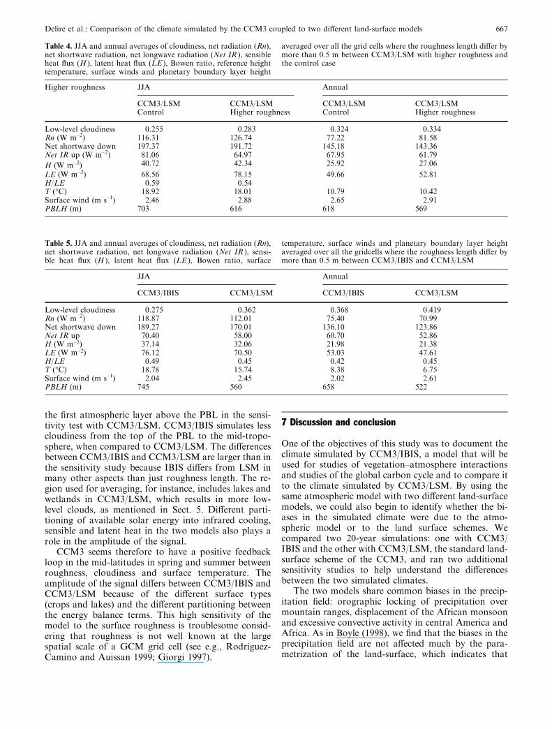
the first atmospheric layer above the PBL in the sensi-tivity test with CCM3/LSM. CCM3/IBIS simulates lesscloudiness from the top of the PBL to the mid-tropo-sphere, when compared to CCM3/LSM. The differencesbetween CCM3/IBIS and CCM3/LSM are larger than inthe sensitivity study because IBIS differs from LSM inmany other aspects than just roughness length. The re-gion used for averaging, for instance, includes lakes andwetlands in CCM3/LSM, which results in more low-level clouds, as mentioned in Sect. 5. Different parti-tioning of available solar energy into infrared cooling,sensible and latent heat in the two models also plays arole in the amplitude of the signal.CCM3 seems therefore to have a positive feedback

loop in the mid-latitudes in spring and summer betweenroughness, cloudiness and surface temperature. Theamplitude of the signal differs between CCM3/IBIS andCCM3/LSM because of the different surface types(crops and lakes) and the different partitioning betweenthe energy balance terms. This high sensitivity of themodel to the surface roughness is troublesome consid-ering that roughness is not well known at the largespatial scale of a GCM grid cell (see e.g., Rodriguez-Camino and Auissan 1999; Giorgi 1997).

7 Discussion and conclusion

One of the objectives of this study was to document theclimate simulated by CCM3/IBIS, a model that will beused for studies of vegetation–atmosphere interactionsand studies of the global carbon cycle and to compare itto the climate simulated by CCM3/LSM. By using thesame atmospheric model with two different land-surfacemodels, we could also begin to identify whether the bi-ases in the simulated climate were due to the atmo-spheric model or to the land surface schemes. Wecompared two 20-year simulations: one with CCM3/IBIS and the other with CCM3/LSM, the standard land-surface scheme of the CCM3, and ran two additionalsensitivity studies to help understand the differencesbetween the two simulated climates.The two models share common biases in the precip-

itation field: orographic locking of precipitation overmountain ranges, displacement of the African monsoonand excessive convective activity in central America andAfrica. As in Boyle (1998), we find that the biases in theprecipitation field are not affected much by the para-metrization of the land-surface, which indicates that

Table 4. JJA and annual averages of cloudiness, net radiation (Rn),net shortwave radiation, net longwave radiation (Net IR ), sensibleheat flux (H ), latent heat flux (LE ), Bowen ratio, reference heighttemperature, surface winds and planetary boundary layer height

averaged over all the grid cells where the roughness length differ bymore than 0.5 m between CCM3/LSM with higher roughness andthe control case

Higher roughness JJA Annual

CCM3/LSM CCM3/LSM CCM3/LSM CCM3/LSMControl Higher roughness Control Higher roughness

Low-level cloudiness 0.255 0.283 0.324 0.334Rn (W m–2) 116.31 126.74 77.22 81.58Net shortwave down 197.37 191.72 145.18 143.36Net IR up (W m–2) 81.06 64.97 67.95 61.79

H (W m–2) 40.72 42.34 25.92 27.06

LE (W m–2) 68.56 78.15 49.66 52.81H/LE 0.59 0.54T (�C) 18.92 18.01 10.79 10.42Surface wind (m s–1) 2.46 2.88 2.65 2.91PBLH (m) 703 616 618 569

Table 5. JJA and annual averages of cloudiness, net radiation (Rn),net shortwave radiation, net longwave radiation (Net IR ), sensi-ble heat flux (H ), latent heat flux (LE ), Bowen ratio, surface

temperature, surface winds and planetary boundary layer heightaveraged over all the gridcells where the roughness length differ bymore than 0.5 m between CCM3/IBIS and CCM3/LSM

JJA Annual

CCM3/IBIS CCM3/LSM CCM3/IBIS CCM3/LSM

Low-level cloudiness 0.275 0.362 0.368 0.419Rn (W m–2) 118.87 112.01 75.40 70.99Net shortwave down 189.27 170.01 136.10 123.86Net IR up 70.40 58.00 60.70 52.86H (W m–2) 37.14 32.06 21.98 21.38LE (W m–2) 76.12 70.50 53.03 47.61H/LE 0.49 0.45 0.42 0.45T (�C) 18.78 15.74 8.38 6.75Surface wind (m s–1) 2.04 2.45 2.02 2.61PBLH (m) 745 560 658 522

Delire et al.: Comparison of the climate simulated by the CCM3 coupled to two different land-surface models 667

they are probably due to the atmospheric model. Bothmodels also share common biases in the temperaturefield in boreal winter when the radiation input is low inthe mid to high latitudes of the Northern Hemisphereand the land, lakes and wetlands are frozen, leaving theatmospheric model the most probable reason for thebiases.Because the radiative forcing is higher from spring

through fall, surface temperature and energy balancedepend largely on the land surface parametrization.With CCM3/IBIS, mean annual temperatures at thelowest atmospheric level are 1.7 �C higher globally thanwith CCM3/LSM. The disagreement is particularly largein the Sahara, Greenland and Antarctica, and in summerover the mid-latitudes of the Northern Hemispherewhere CCM3/IBIS simulates drier, hotter and lesscloudy conditions. Albedo and/or snow parametrizationdifferences between the two models explain most of theSahara and high-latitude temperature disagreement. Oursensitivity study shows that the presence of lakes andwetlands in CCM3/LSM can account for about half ofthe difference in temperature in summer over the lakeand wetland regions of the mid-latitudes. According toBonan (1999), the presence of crops in CCM3/LSM canalso explain part of temperature difference in the mid-latitudes. Finally, we showed with a second sensitivitystudy that differences in roughness length between thetwo models explain about a third of summer surfacetemperature difference through a feedback mechanismlinking surface wind speed, planetary boundary layerheight, low-level cloudiness and radiation. This indicatesthat with the two models used here, the vegetation in-fluences the climate not only through its albedo andevapotranspiration but also through its roughness.The results of this comparison indicate several ways

to improve both CCM3/IBIS and CCM3/LSM. Forexample, to better represent present-day climate, weneed to include a representation of crops, lakes andwetlands in CCM3/IBIS. We also need to further ana-lyze the validity of the roughness length parametrizationin the model. In CCM3/LSM, we need to correct theprescribed albedo of the Sahara and investigate thecauses of the continental scale cold bias in Eurasia insummer. We also need to refine the parametrization oflakes and wetlands and further investigate the impor-tance of lake depths on the local climate.

Acknowledgements We thank Marcos Heil Costa, David Pollard,Peter Snyder and Starley Thompson for valuable discussion andcomments on the manuscript. This work was supported by theNational Science Foundation’s ‘‘Methods and Models for Inte-grated Assessment’’ program.

References

Amthor JS (1984) The role of maintenance respiration in plantgrowth. Plant, Cell Environ 7: 561–569

Bonan G (1996) A land surface model (LSM version 1.0) forecological, hydrological, and atmospheric studies: technical

description and user’s guide. National Center for AtmosphericResearch, Boulder, CO, USA

Bonan GB (1995a) Land–atmosphere CO2 exchange simulated by aland surface process model coupled to an atmospheric generalcirculation model. J Geophys Res 100(D2): 2817–2831

Bonan GB (1995b) Sensitivity of a Gcm simulation to inclusion ofinland water surfaces. J Clim 8 (11):2691–2704

Bonan GB (1998) The land surface climatology of the NCAR LandSurface Model coupled to the NCAR Community ClimateModel. J Clim 11(6): 1307–1326

Bonan GB (1999) Frost followed the plow: impacts of deforestationon the climate of the United States. Ecol Appl 9(4): 1305–1315

Botta A, Viovy N, Ciais P, Friedlingstein P, Monfray P (2000) Aglobal prognostic scheme of leaf onset using satellite data.Global Change Biol 6(7): 709–725

Boyle JS (1998) Evaluation of the annual cycle of precipitation overthe United States in GCMs: AMIP simulations. J Clim 11(5):1041–1055

Braconnot P (2000) PMIP, Paleoclimate Modeling Intercompari-son Project (PMIP): Proc 3rd PMIP workshop, Canada.WCRP-111, WMO/TD-1007

Brostrom A, Coe M, Harrison SP, Gallimore R, Kutzbach JE,Foley J, Prentice IC, Behling P (1998) Land surface feedbacksand palaeomonsoons in northern Africa. Geophys Res Lett25(19): 3615–3618

Charney JG (1975) Dynamics of deserts and drought in the Sahel.Q J R Meteorol Soc 101: 193–202

Cogley JG (1991) GGHYDRO – Global hydrological data release2.0. Trent Climate Note 91-1, Trent University – Department ofGeography, Peterborough, Ontario, Canada

Collatz GJ, Ball JT, Grivet C, Berry JA (1991) Physiological andenvironmental-regulation of stomatal conductance, photosyn-thesis and transpiration – a model that includes a laminarboundary-layer. Agr Forest Meteorol 54(2–4): 107–136

Collatz GJ, Ribas-Carbo M, Berry JA (1992) Coupled photosyn-thesis-stomatal conductance model for leaves of C4 plants. AustJ Plant Physiol 19: 519–538

Cox PM, Betts RA, Jones CD, Spall SA, Totterdell IJ (2000) Ac-celeration of global warming due to carbon-cycle feedbacks in acoupled climate model. Nature 408(6813): 750–750

Dorman JL, Sellers PJ (1989) A global climatology of albedoroughness length and stomatal resistance for atmospheric gen-eral circulation models as represented by the simple biospheremodel (SiB). J Appl Meteorol 28: 833–855

Farquhar GD, von Caemmerer S, Berry JA (1980) A biochemicalmodel of photosynthetic CO2 assimilation in leaves of C3 spe-cies. Planta 149: 78–90

Foley JA, Levis S, Costa MH, Cramer W, Pollard D (2000) In-corporating dynamic vegetation cover within global climatemodels. Ecol Appl 10(6): 1620–1632

Foley JA, Levis S, Prentice IC, Pollard D, Thompson SL (1998)Coupling dynamic models of climate and vegetation. GlobalChange Biol 4(5): 561–579

Foley JA, Prentice CI, Ramankutty N, Levis S, Pollard D, Sitch S,Haxeltine A (1996) An integrated biosphere model of landsurface processes, terrestrial carbon balance, and vegetationdynamics. Global Biogeochem Cycles 10(4): 603–628

Gates WL (1992) The Atmospheric Model Intercomparison Pro-ject. Bull Am Meteorol Soc 73: 1962–1970

Gates WL, Boyle JS, Covey C, Dease CG, Doutriaux CM, DrachRS, Fiorino M, Gleckler PJ, Hnilo JJ, Marlais SM, Phillips TJ,Potter GL, Santer BD, Sperber KR, Taylor KE,Williams DN(1999) An overview of the results of the Atmospheric ModelIntercomparison Project (AMIP I). Bull Am Meteorol Soc80(1): 29–55

Giorgi F (1997) An approach for the representation of surfaceheterogeneity in land surface models. 1. Theoretical framework.Mon Weather Rev 125(8): 1885–1899

Groisman PY, Bradley RS, Sun BM (2000) The relationship ofcloud cover to near-surface temperature and humidity: com-parison of GCM simulations with empirical data. J Clim 13(11):1858–1878

668 Delire et al.: Comparison of the climate simulated by the CCM3 coupled to two different land-surface models

Hack JJ, Kiehl JT, Hurrell JW (1998) The hydrologic and ther-modynamic characteristics of the NCAR CCM3. J Clim 11(6):1179–1206

IGBP-DIS (1999) Global soil data task: spatial database of soilproperties. International Geosphere–Biosphere Programme –Data and Information System, Toulouse, France

Jones HG (1992) Plants and microclimate: a quantitative approachto environmental plant physiology. Cambridge UniversityPress, Cambridge, UK, pp 428

Kiehl JT, Hack JJ, Bonan GB, Boville BA, Williamson DL, Rasch PJ(1998) The National Center for Atmospheric Research Com-munity Climate Model: CCM3. J Clim 11(6): 1131–1149

Kucharik CJ, Foley JA, Delire C, Fisher VA, Coe MT, Lenters JD,Young-Molling C, Ramankutty N, Norman JM, Gower ST(2000) Testing the performance of a dynamic global ecosystemmodel: water balance, carbon balance, and vegetation structure.Global Biogeochem Cycles 14(3): 795–825

Levis S, Foley JA, Pollard D (1999a) CO2, climate, and vegetationfeedbacks at the Last Glacial Maximum. J Geophys Res Atmos104(D24): 31,191–31,198

Levis S, Foley JA, Pollard D (1999b) Potential high-latitude veg-etation feedbacks on CO2-induced climate change. GeophysRes Lett 26(6): 747–750

Levis S, Foley JA, Pollard D (2000) Large-scale vegetation feed-backs on a doubled CO2 climate. J Clim 13(7): 1313–1325

New M, Hulme M, Jones P (1999) Representing twentieth-centuryspace-time climate variability. Part I: development of a 1961–90mean monthly terrestrial climatology. J Clim 12(3): 829–856

Olson JS, Watts JA, Allison LJ (1983) Carbon in live vegetation ofmajor world ecosystems. ORNL-5862, Oak Ridge NationalLaboratory, Oak Ridge, Tenn, USA

Pollard D, Thompson SL (1993) Description of a land-surface-transfer model (LSX) as part of a global climate model.National Center for Atmospheric Research, Boulder, CO, USA

Qu WQ, Henderson-Sellers A (1998) Comparing the scatter inPILPS off-line experiments with that in AMIP I coupledexperiments. Global Planet Change 19(1–4): 209–223

Ramankutty N, Foley JA (1999) Estimating historical changesin global land cover: croplands from 1700 to 1992. GlobalBiogeochem Cycles 13(4): 997–1027

Rodriguez-Camino E, Avissar R (1999) Effective parameters forsurface heat fluxes in heterogeneous terrain. Tellus Ser a-dynMeteorol Oceanogr 51(3): 387–399

Sellers PJ, Randall DA, Collatz GJ, Berry JA, Field CB, DazlichDA, Zhang C, Collelo GD, Bounoua L (1996) A revised landsurface parametrization (SiB2) for atmospheric GCMs. 1.Model formulation. J Clim 9(4): 676–705

Sud YC, Shukla J, Mintz Y (1988) Influence of land surface-roughness on atmospheric circulation and precipitation –a sensitivity study with a general-circulation model. J ApplMeteorol 27(9): 1036–1054

Texier D, de Noblet N, Braconnot P (2000) Sensitivity of theAfrican and Asian monsoons to mid-Holocene insolationand data-inferred surface changes. J Clim 13(1): 164–181

Thompson SL, Pollard D (1995a) A global climate model (GEN-ESIS) with a land-surface transfer scheme (lsx). Part II: CO2sensitivity. J Clim 8(5): 1104–1121

Thompson SL, Pollard D (1995b) A global climate model (GEN-ESIS) with a land-surface-transfer scheme (LSX). Part 1: pre-sent-day climate. J Climatel 8: 732–761

Vogelzang DHP, Holtslag AAM (1996) Evaluation and modelimpacts of alternative boundary-layer height formulations.Boundary-Layer Meteorol 81: 245–269

Webb RS, Rosenzweig CE (1993) Specifying land surface charac-teristics in general circulation models: soil profile data set andderived water-holding capacities. Global Biogeochem Cycles7(1): 97–108

Delire et al.: Comparison of the climate simulated by the CCM3 coupled to two different land-surface models 669