1

Efforts at Comparing Simulated and Observed Fire Growth Patterns

Final Report 2/25/2000

INT-95066-RJVA

Mark A. Finney Systems for Environmental Management

PO BOX 8868 Missoula MT 59802

Abstract Data on fire growth were collected for 21 fires in the western US. Some of the data sets were complete (included spatial GIS themes for fuels and topography as well as observed weather and fire growth) and others were missing some components and were not useable. These data were intended for use as comparisons for the fires simulated with FARSITE. After attempting to use these data for comparisons, however, I found it impossible to verify the accuracy of the different data types (e.g. fuels maps, weather observations, mapped fire perimeters). Accuracy itself is probably not possible to define for many of the variables used for the simulations (e.g. windspeed, fuel model, spread rate); the time and space scales that these variables are measured is different from the scales of the phenomena themselves. The comparisons of observed and predicted fire patterns are therefore not easily interpreted -- the cause(s) of good or bad agreement cannot be used to infer the "validity" or accuracy of the model separately from the accuracy of the data. A qualitative visual analysis suggests general level agreement between the predicted and observed trends for many fires. Introduction The fire growth model FARSITE (Finney 1998) has been used for several years for wildland fire growth simulation. Originally, FARSITE was used for long-range projection (beyond the accuracy of weather forecasts) for examining the sensitivity of fire growth to potential weather scenarios. More recent uses have stressed the need for simulations in fire planning as well as short-medium range projections for use in tactical decision making for firefighting operations. The question naturally arises “how well does FARSITE simulate what happens on actual fires?” To date, the answer has relied on intuitive reasoning. FARSITE merely implements existing models that have been applied individually for many years. If these separate models are adequate, then FARSITE should produce at least the same level of utility as those models individually. Another line of reasoning comes from preliminary evidence (Finney 1994, Finney and Ryan 1995, Finney and Andrews 1998) and from operational uses of FARSITE on active fires. Past simulations have shown that when input data were reasonably accurate and the model

2

assumptions were met by the type of fire being modeled, then the outputs were accurate to a useful level (Finney and Ryan 1995). It is desirable, however, to address the question of model validity or usefulness in a more objective and thorough fashion. This report describes the results of some simulations and the comparisons with the observed fire growth data. In many cases, some portions within a fire will display obvious agreement but others will show disagreement. The comparisons are annotated to provide background information about the fire and known or suspected reasons for the simulation outcomes. Methods Fire growth modeling has long sought to describe and reproduce the observed patterns of fire growth (Hornby 1936, Fons 1946, Byram 1959). The effort began with the application of a single fire shape, such as the ellipse (Van Wagner 1969, Bratten 1978), double ellipse (Albini 1976, Anderson 1983), or ovoid (Peet 1967) to fires in uniform environmental conditions. These fire shape models relate windspeed to the eccentricity of fires (Alexander 1985, Anderson 1983, Bilgili and Methven 1990, McAlpine and Wakimoto 1991). They have provided the foundation for more recent computerized fire growth models that reproduce the basic fire shapes along a given fire edge to propagate the fire front in uniform and non-uniform conditions (Kourtz and O’Regan 1971, Sanderlin and Sunderson 1975, Anderson et al. 1982, Richards 1990). The process of testing the utility of a fire growth model has traditionally involved visual comparisons between the observed and predicted. This is a practical measure that will always be used when models are exercised operationally. Sometimes this comparison process is referred to as “validation”. With the simple fire shapes it is usually obvious as to the degree of agreement between the modeled and observed fire pattern (Anderson 1983) because temporal and spatial conditions are assumed essentially constant. Comparisons can be made for the whole fire without regard to local variations in time or space. With fire growth models, however, the assumptions of a uniform fire environment are intentionally abandoned, because it is desired for the models to work where fuels, weather, and topography are heterogeneous. Testing models under these conditions therefore becomes more difficult because comparisons must address agreement that is time and space dependent. The subject of “validation” is often confusing because a model’s purpose, performance criteria, and usage is often poorly specified (Rykiel 1996). Depending on the type of model, validation has different uses for practical models than for theoretical models (Rykiel 1996). Validation of a practical model should test acceptability of a model for its intended uses. Validation of theoretical models tries to establish the reliability of inferences made about system behavior based on the model. FARSITE is a model with both practical and theoretical uses. Despite its practical origins, FARSITE does serve as a test of theoretical issues concerning fire behavior modeling. Foremost is the assemblage of the different fire behavior models in a single simulation that has revealed some interesting consequences arising from the spatial implementation of models for surface, crown, and spot fire (Finney 1998). Many of these tests have suggested that predicted fire growth patterns do meet with basic expectations of fire growth (e.g. French 1992); some tests identify weaknesses in fire behavior models. On the practical

3

side, FARSITE has become widely used for operational prediction of fire growth of active wildland fires as well as for modeling in support of planning for potential fires. Clearly, some attempt to measure the fidelity of modeled fire growth with respect to real wildland fires is needed. The reasons for this validation are to 1) assist interpretations and clarify a realistic range of expectations of fire modeling, 2) to establish some procedures by which agreement is tested and perhaps improved, and 3) explicate the consequences of data quality on model performance. Objective methods for comparison of modeled with observed fire patterns is made difficult by the time and space dependency of these patterns. Green et al. (1983) used a regression technique to compare radial fire spread distances from point of origin, relying on r2 as the measure of agreement. This technique was adequate for relatively simple convex fires without complex conditions that cause spread along curving routes away from the ignition point. It is less logical where fire growth occurs over many days or weeks and shapes become complex by such indirect spread. Finney (1994, 1995) compared observed and predicted radial spread (similar to Green et al. 1983), area overlap, and perimeter length. The same limitations were present here as in (Green et al. 1983) and none of these methods could be considered adequate for reflecting time and space dependent trends of agreement that were obvious by a visual comparison of maps showing predicted and observed fire growth patterns. Perry et al. (1999) used an index (Sorensen coefficient) to assess the agreement of a fire simulation. This index still is based on areas observed and predicted but excludes a time and space dependencies that are critical to the comparison. Visual comparison is most often used (Sanderlin and Van Gelder 1977, Anderson et al. 1982, Finney 1994, Finney 1995, Xu and Lathrop 1994, Coleman and Sullivan 1996). Although subjective, the level of agreement is readily discerned. A statistical measure of agreement, the kappa statistic, has been used for comparing and detecting change in vegetation maps (Monserud and Leemans 1993). It initially showed promise for comparing fire patterns as well. It relies on cell by cell comparison between categories of two maps to form a matrix. The matrix of categories contains the number of cells with a given attribute on the observed and predicted maps:

Observed Predicted 1 2 3 4 5 6 7 8 9 totals 1 3 3 6 2 2 3 3 3 1 12 3 4 5 3 3 15 4 3 6 7 3 1 1 21 5 1 7 8 9 9 4 38 6 9 9 9 4 4 35 7 1 4 4 4 4 17 8 1 4 4 4 13 9 4 4 4 12 totals 7 13 22 30 24 23 20 18 12 169 For fire patterns, the categories 1-9 (above) would correspond to different time periods of fire growth (or regions of the fire perimeter). The column, row, and grand totals are used to compute

4

a percentage matrix that is used to compute the kappa statistic. The kappa statistic ranges from approximately 0 (no agreement) to 1.0 (perfect agreement). Good agreement would be depicted by a high concentration of values along the diagonal of the above matrix. In preliminary analyses, I explored the use of kappa for fire pattern comparison but found several problems that forced me to abandon it. First, the extent of the relevant landscape could not be determined objectively. Although the predicted and observed fire boundaries are definite, some area surrounding their joint coverage must be included in computing the Kappa. This surrounding area was not observed to have burned and also not predicted. The relevance of this surrounding area decreases with distance away from the fire edge. In other words, a successful fire projection would not predict fire to occur where it was not observed; at some distance away from the fire (say 10 miles) it becomes ludicrous to consider these areas as a prediction success (we know the fire won’t get there). Thus, the Kappa statistic improves as more landscape area is included surrounding the joint boundary of the predicted and observed fires; it represents a larger proportional area that was “predicted correctly” as not having been burned. Second, finer temporal divisions in fire growth make the comparison more sensitive to asynchroneity in fire projections. Although greater temporal resolution is desired for comparing trends in fire growth maps, this penalizes the Kappa statistic because slight time displacements occurring between observed and predicted fire arrival times result in zero agreement among map categories. For example, a simulated fire that over or under-predicted fire growth by exactly 1 time period would result in a very low Kappa, even if it exactly matched the spatial pattern of observed fire growth (just lagged by 1 period). Thus, the more highly resolved the fire progression map, the generally worse the Kappa statistic. Without a work-around, these shortcomings appeared to offset any advantage in objectivity gained by using the Kappa because there was no way to interpret the resulting Kappa value. Despite the possibility that better analyses exist, such as Fourier decomposition of fire images, the methods used here for comparing observed and predicted fire patterns were entirely subjective. This was decided because the tests that ultimately matter most to field users of FARSITE will also be visual and subjective. They will decide by visual inspection if they see enough similarity to the real fire or not. Few practitioners of fire growth modeling will use anything more complex to decide whether the model is useful or not for a particular purpose. Results The data sets used for comparisons came primarily from National Parks (Table 2) and wilderness areas. Most of the fires occurred in mixtures of timber-type fuels and were surface fires. Many fires in the Sierra Nevada Mountains contained mixtures of brush and forest fuels. One fire (South Canyon) was a wildfire solely in brush fuels. Many fires contained missing critical data components (weather data, fuels data etc.) and could not be used.

5

Fire Name Location Dates Sprsn Fuels/Fire Mill Creek Ochoco NF 9/1995 Y 8,9,10, surface Horizon Yosemite NP 6-9/1994 Y 1/5/8/9/10, surface Howling Glacier NP 6-9/1994 Y 8/surface, smoldering Redbench Glacier NP 9/1988 Y 10/12, crownfire Topanga Canyon Los Padres NF 11/1993 Y 2/4/5, chaparral Deer Creek Sequoia NP 10/1991 N 5/8/10, surface Avalanche Sequoia NP 8/1989 N 5/8/9/10, surface Rattlesnake Sequoia NP 7/1992 N 5/8/10,,surface Buck Peak Sequoia NP 8/1995 N 5/8/9/10, surface Castle Complex Sequoia NP 7/1996 N 5/8/10, surface Ackerson Complex Yosemite NP 8/1996 Y 2/5/8/9/10, surf-crown Rogge Eldorado NF 8/1996 Y 2/5/10, surf-crown Elbow Basin Okanagan NF 8/1996 N 8/9/10, surface-torch Bee San Jacinto NF 6/1996 Y 4/5, chaparral Hatchery Complex Wenatchee NF 7/1994 Y 8/9/10, crown-surf Frog Yosemite NP 8/1990 N 8/9/10, surf Buckeye Sequoia NP 8/1990 Y 4/5, chaparral Little Gabbro Lake Boundary Waters, MN 6/1995 N 8,9,10, surf-crown Whitefeather Lake Boundary Waters, MN 6/1996 N 8,9,10, surf-crown Kootenai Complex Glacier NP 9/1998 N 10,12, crown-surf South Canyon Colorado 7/1994 Y 2,4, surf Visual comparisons are presented for 9 of the fires listed above (Figure 1-9). Comparisons have already been published for the Deer Creek Fire (Finney 1994, 1995), Avalanche (Finney 1995), and Horizon and Howling (Finney and Ryan 1995, Finney and Andrews 1998). The simulations shown here are for the entire fire duration, starting with the earliest fire perimeter and ending with the latest. This produces the greatest discrepancy between observed and predicted because of the compounding of errors over time. In other words, calculations made later in the simulation are based on the location and behavior of the fire simulated previously that itself contains inaccuracies. When FARSITE is used for making projections on active fires, the forecasted simulations are always updated by starting from the latest known perimeter to reduce error. Discussion The objective for validation is to discern model performance or error. This is not possible, regardless of how "validation" is defined (Rykiel 1996), if the error of the input data or observed data used for comparison are not controlled or known. In the absence of controlled error for inputs and observations, the results of any comparison cannot be interpreted as to the cause (s). The same conclusions were reached after attempts to validate the Rothermel (1972) spread equation as implemented in the program FIREMOD for surface fire spread (Albini and Anderson

6

1982). Here, comparisons are presumed to be considerably simpler than attempted for FARSITE because there are no explicit spatial or temporal variations in the fire behavior models or data. However, after attempting to "validate" FIREMOD and noting numerous problems with the data, Albini and Anderson (1982) concluded with respect to "Model Integrity vs. Input Data Accuracy" that:

"Attempts to evaluate the theoretical fire behavior models described above through operation or field-level experiment resulted in unclear definitions of the reasons for output inconsistencies. It is impossible for the most part to isolate the cause of output variations to either the accuracy or resolution of the input data, applicability of the model to the real world, or (in some cases) to errors which may have crept into the program during the implementation process. Even in the simplest model, FIREMOD, complex relationships between input data readily available to field personnel and internal model parameters exist. This makes it extremely difficult to evaluate which input variable is suspect when deviations are noted between predicted and actual fire behavior characteristics." (Albini and Anderson 1982)

Certainly, all of the problems encountered by Albini and Anderson (1982) are present in the data sets assembled for these comparisons. All data sets, even those I collected personally, had questionable accuracy that seriously compromised their uses for a rigorous validation. None of the fuels or weather data could be verified. Practically, this is impossible across vast landscapes -- to measure at multiple scales the fuel conditions and weather and wind variables. Theoretically, it is also impossible at this time to define precisely the fuel conditions as they vary from the stylized fuel models used to approximate them or what is really meant by wind speed and direction (as used in the fire models and measured in the field). The fuel models (Anderson 1982) are commonly used to approximate the burning characteristics of real wildland fuels and to populate maps of fuel conditions across landscapes. They are not necessarily used to represent the structural characteristics of those fuels. Thus, the real surface fuels often contain so much structural variation at many scales (and burn differently too) that their correspondence to the stylized model is completely subjective and not quantifiable. Wind speed and direction vary at many scales in time and space that are not captured for a large fire by a single weather station or by field observers using hand-held measuring devices. Even if high resolution temporal or spatial records of winds were available, the fire models assume a constant "midflame" wind that relates in an unknown way to the real pattern of variation of the measurements. This serves to emphasize the need for research into effects of variability on the use of fire behavior models individually. The observed fire data in these data sets also contain an unknown level of error that varies both spatially, temporally, and between fires. Fire perimeter data for all data sets were obtained from management records. Most fire perimeters were obtained by direct observation from the air or ground and drawn by hand. Some perimeters on some fires were obtained from infrared photographs. All of the fires were mapped to a level of accuracy that served the decision making by managers of those fires and not to a level required for rigorous validation of fire models. Many perimeters have a very coarse time-resolution of a single day (or multiple days) with no record of the hour of the observation. The long time intervals between observations can be belie

7

important details of how the fire moved during that period, especially for fast moving fires that encounter variable conditions (fuels, topography, change in weather conditions etc.) between recorded observations. These variable conditions can cause the fire to move faster along indirect routes than would be inferred as the most direct route from the fire progression map. The perimeter of a large fire may be mapped by several individuals at different times and assembled later as a composite with guesses and interpolation used for perimeter segments that were not directly observed. Fire perimeters are often assumed rather than observed because they cannot be seen through the smoke or because spot fires are recorded as the outer edge of the front. This leads to errors, sometimes on the order of kilometers, that result in shrinking fire acreage over time (later fire maps indicate smaller fires than previously documented). In many cases, fire suppression had effects on progression, either stopping, delaying, or accelerating fire growth (burnout). Water drops from aircraft are often used to delay fires by extinguishing spots or other flanks of the main fire. Natural barriers within the fire management area (streams, roads, ridges) are often fortified by suppression crews to delay the fire. These have very specific effects on the fire growth (in time and space) that are never documented and cannot be inferred from studying a fire progression map. These activities change the fire shape but more importantly, they disrupt the temporal progress of the fire growth that is not knowable during validation. The amount of agreement between predictions and observations tends to improve as the fire becomes larger. This has been consistently observed in the use of FARSITE and was obvious in these comparisons as well. This happens because the fire becomes less sensitive to small-scale variations or heterogeneity in the fuels and weather that are very influential to fires with sizes at that same general scale. As the fire becomes larger, it essentially represents a larger sampling of the landscape and has a greater probability of encountering fuels and wind conditions that are favorable, irrespective of local areas that retard its growth. Conclusions Clearly, the pervasive lack of control over input data precluded any attempt to perform a rigorous validation of fire behavior models, FARSITE or its components. FARSITE appears to be capable of producing reasonable fire growth characteristics for many fires but requires considerable judgement on the part of the user to interpret the available input data and make adjustments as necessary. These requirements are consistent with the recommended use of all fire behavior models (BEHAVE), some of which are the component models in FARSITE.

8

Further attempts to establish the accuracy of FARSITE or other fire behavior models for field uses are probably futile without serious improvements in data definition and collection. If objective and quantitative model comparisons are desirable, then a concentrated effort is needed to: 1. first define precisely the level of acceptable performance for the models (spatial and

temporally), 2. then identify the data and their precision needed to test this for the particular models, 3. develop quantitative and objective means for doing the testing, 4. and finally to collect data expressly for the validation purpose. Even if models are shown to be acceptable and "accurate" for a given use, the nature of fire behavior modeling permits a broad opportunity for error in field uses of the models. Whether any model is useful or not will, in large measure, depend on the qualifications of the users.

9

Literature Cited Albini, F.A. 1976. Estimating wildfire behavior and effects. USDA For. Serv. Gen. Tech. Rep.

INT-30. Albini, F.A., and E.B. Anderson. 1982. Predicting fire behavior in U.S. Mediterranean

ecosystems. In E.C. Conrad and W.C. Oechel. Proc. of the symp. on Dynamics and management of Mediterranean-Type ecosystems. USDA For. Serv. Gen. Tech. Rep. PSW-58.

Alexander, M.E. 1985. Estimating the length-to-breadth ratio of elliptical forest fire patterns.

pp. 287-304 Proc. 8th Conf. Fire and Forest Meteorology. Anderson, H.E. 1983. Predicting wind-driven wildland fire size and shape. USDA For. Serv.

Res. Pap. INT-305. Anderson, D.G, E.A. Catchpole, N.J. DeMestre, and T. Parkes. 1982. Modeling the spread of

grass fires. J. Austral. Math. Soc. (Ser. B.) 23:451-466. Bilgili, E and I.R. Methven. 1990. The simple ellipse: A basic growth model. 1st Intl. Conf. on

Forest Fire Research, Coimbra 1990. pp B.18-1 to B.18-14. Byram 1959. Chapter Three, Combustion of Forest Fuels. in Davis, .K.P., Forest Fire: Control

and Use. McGraw-Hill. New York. Bratten, F.W. 1978. Containment tables for initial attack on forest fires. Fire Tech. 14(4):297-

303. Colemen, J.R. and A.L. Sullivan. 1996. A real-time computer application for the prediction of

fire spread across the Australian landscape. Simulation 67 (4):230-240. Finney, M.A. 1994. Modeling the spread and behavior of prescribed natural fires. In:

Proceedings of the 12th Conference on Fire and Forest Meteorology, October 26-28, 1993, Clarion Resort Buccaneer, Jekyll Island, GA, Society of American Foresters, Bethesda MD, SAF publication 94-02. 138-143.

Finney, M.A. 1995. Fire growth modeling in the Sierra Nevada of California. In: J.K. Brown,

R.W Mutch, C.W. Spoon, and R.H. Wakimoto. Proc. Symp. on Fire in Wilderness and Park Management. Missoula MT March 30-April1 1993. Pp 189-191.

Finney, M.A. 1998. FARSITE: Fire Area Simulator - Model development and evaluation.

USDA For. Serv. Research Paper RMRS-RP-4. 47 p. Finney, M.A. and K.C. Ryan. 1995. Use of the FARSITE fire growth model for fire prediction

in US National Parks. Proc. The International Emergency Mgt. and Engineering Conf. May 1995 Sofia Antipolis, France. pp 186-

10

Finney, M.A. and P.L. Andrews. 1998. The FARSITE fire area simulator: fire management applications and lessons of summer 1994. Proc. Intr. Fire Council Mtg. November 1994, Coer D’Alene ID.

Fons, W.T. 1946. Analysis of fire spread in light forest fuels. J. Agric. Res. 72(3):93-121. French, I.A. 1992. Visualisation techniques for the computer simulation of bushfires in two

dimensions. M.S. Thesis University of New South Wales, Australian Defence Force Academy, 140 pages.

Green, D.G., A.M. Gill, and I.R. Noble. 1983. Fire shapes and the adequacy of fire-spread

models. Ecol. Mod. 20:33-45. Hornby, L.G. 1936. Fire control planning in the Northern Rocky Mountain region. Prog. Rep.

1. USDA For. Serv. Ogden UT., 179p. Kourtz, P. and W.G. O'Reagan. 1971. A model for a small forest fire.. to simulate burned and

burning areas for use in a detection model. For. Sci. 17(2):163-169. McAlpine, R.S. and R.H. Wakimoto. 1991. The acceleration of fire from point source to

equilibrium spread. For. Sci. 37(5):1314-1337. Monserud, R.A. and R. Leemans. 1993. Comparing global vegetation maps with the Kappa

statistic. Ecol Modl. 62:275-293. Perry, L.W.G., A.D. Sparrow, and I.F. Owens. 1999. A GIS-supported model for the simulation

of the spatial structure of wildland fire, Cass Basin, New Zealand. J. Appl. Ecol. 36:502-518.

Richards, G.D. 1990. An elliptical growth model of forest fire fronts and its numerical solution.

Int. J. Numer. Meth. Eng. 30:1163-1179. Rykiel, E.J., 1996. Testing ecological models: the meaning of validation. Ecol. Modl. 90:229-

244. Sanderlin, J.C. and J.M. Sunderson. 1975. A simulation for wildland fire management planning

support (FIREMAN): Volume II. Prototype models for FIREMAN (PART II): Campaign Fire Evaluation. Mission Research Corp. Contract No. 231-343, Spec. 222. 249 pages.

Sanderlin, J.C. and R. J. Van Gelder. 1977. A simulation of fire behavior and suppression

effectiveness for operation support in wildland fire management. In: Proc. 1st Int. Conv. on mathematical modeling, St. Louis, MO. pp 619-630.

Van Wagner, C.E. 1969. A simple fire growth model. Forestry Chron. 45:103-104.

11

Xu, J. and R.G. Lathrop. 1994. Geographic information system based wildfire spread simulation. Proc. 12th Conf. Fire and Forest Meteorology, pp 477-484.

Figure 1. Ackerson Wildfire 30,000 ac (Yosemite NP 1996)

Observed 8/14-8/23/1996 Predicted

5 miles

Figure 2. Millcreek Prescribed Natural Fire 1200 ac(Prineville Oregon 1995)

9/17/1995

9/18/1995

9/19/1995

9/20/1995

9/21/1995

9/22/1995

9/23/1995

9/24/1995

9/25/1995

Predicted

1 mile

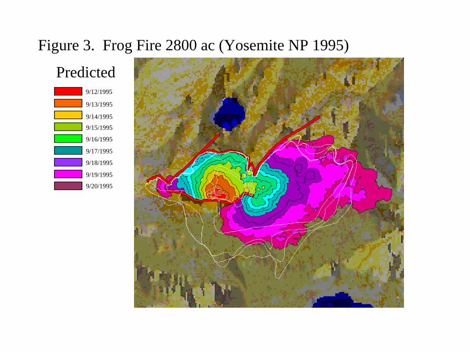
Figure 3. Frog Fire 2800 ac (Yosemite NP 1995)

9/12/1995

9/13/1995

9/14/1995

9/15/1995

9/16/1995

9/17/1995

9/18/1995

9/19/1995

9/20/1995

Predicted

Figure 4. Redbench wildfire 31,000 ac (Glacier NP 1988)

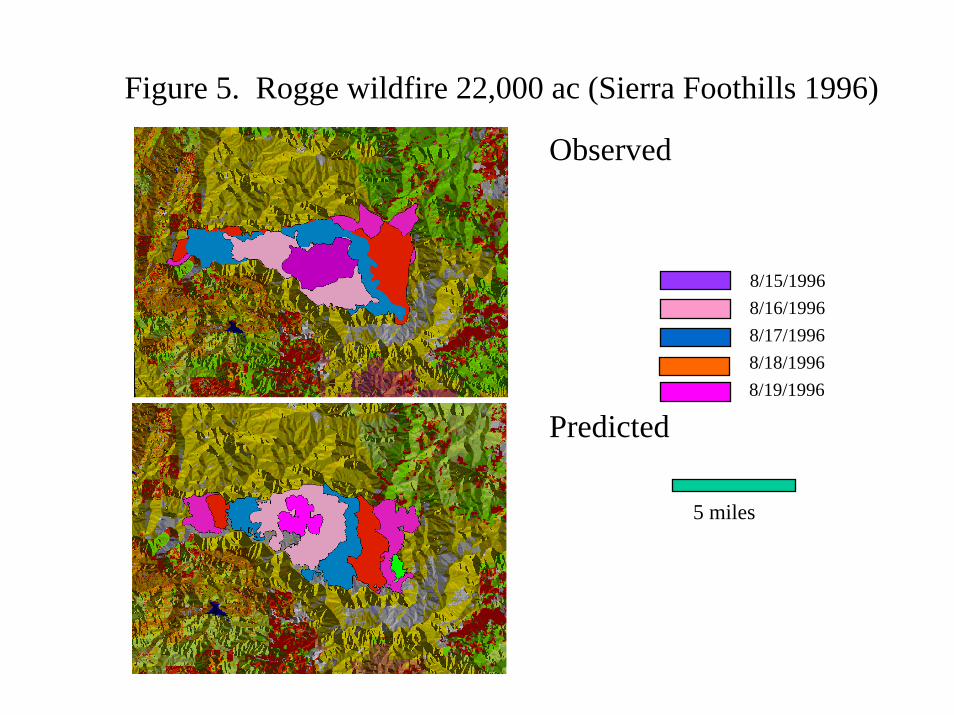
Figure 5. Rogge wildfire 22,000 ac (Sierra Foothills 1996)

Observed

Predicted

8/15/19968/16/19968/17/19968/18/19968/19/1996

5 miles

Figure 6. South Canyon Fire (Colorado) 1994.

XX

Predicted (1min time increments)

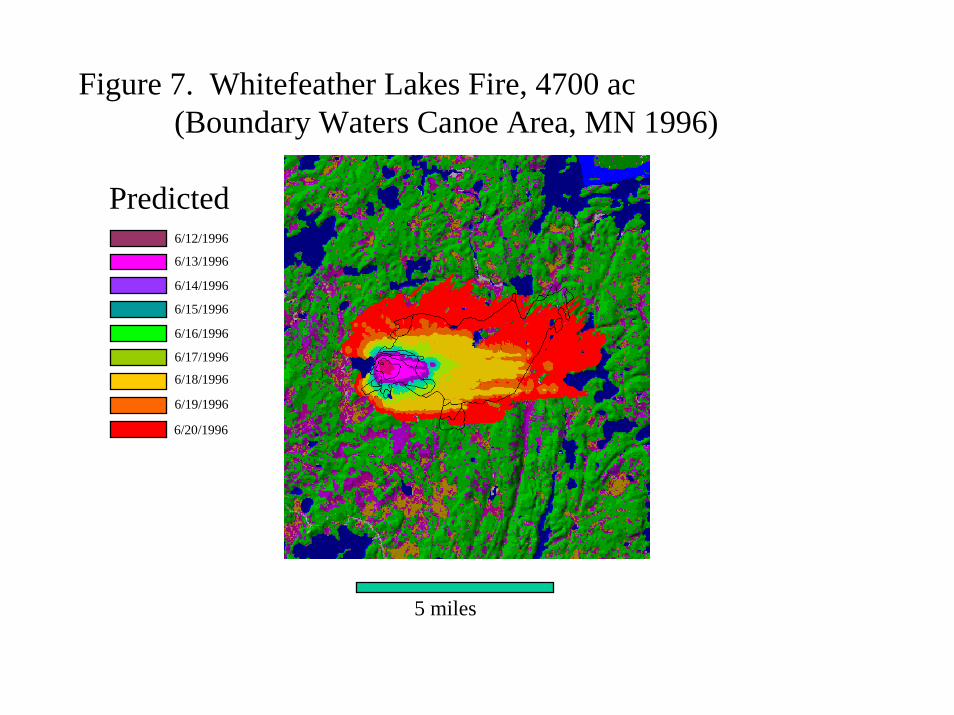
Figure 7. Whitefeather Lakes Fire, 4700 ac(Boundary Waters Canoe Area, MN 1996)

6/12/1996

6/13/1996

6/14/1996

6/15/1996

6/16/1996

6/17/1996

6/18/1996

6/19/1996

6/20/1996

Predicted

5 miles

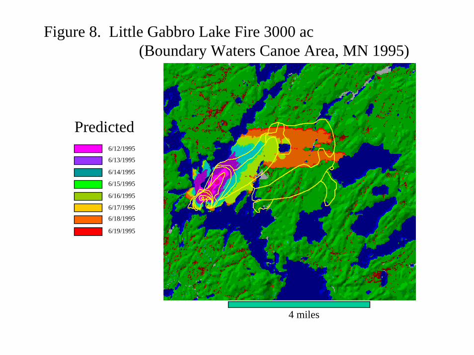
Figure 8. Little Gabbro Lake Fire 3000 ac(Boundary Waters Canoe Area, MN 1995)

Predicted6/12/1995

6/13/1995

6/14/1995

6/15/1995

6/16/1995

6/17/1995

6/18/1995

6/19/1995

4 miles

Figure 9. Koonenai Complex 8000 ac. (Glacier NP 1998)

Predicted 9/4/1998

9/5/1998

9/6/1998