COMPARISON OF MOMENTUM AND VORTEXMETHODS FOR THE AERODYNAMIC

ANALYSIS OF WIND TURBINES

Sandeep Gupta∗ J. Gordon Leishman†

Department of Aerospace Engineering

Glenn L. Martin Institute of Technology

University of Maryland

College Park, Maryland 20742.

An understanding of the blade-element momentum (BEM) theory in comparison with the free-vortexmethod (FVM) has been developed for the analysis of wind turbine aerodynamics. Understanding the limita-tions of BEM methods, used often by the wind turbine community, is very important for the better predictionof turbine power output and blade loads. The BEM theory has been revisited and is compared with vortexmethods. The work shows the limits of applicability of the BEM methods and the better flexibility of the FVMto predict the aerodynamics of a wind turbine for a full range of wind turbine operating states including thevortex ring state, for turbulent wake state and for yawed flow conditions. It is also shown that linear inflowmodels used in conjunction with the BEM theory may not be applicable for higher yaw angles. A universalpower and thrust coefficient curve with the axial induction factor has also been derived to help understand theoperating flow states of a wind turbine over which the FVM can be applied.

Nomenclature

a Axial induction factor, vi/V∞

a′ Tangential induction factor, vt/ΩrA Area of the rotor disk, m2

c Blade chord, mCl Lift coefficientClα Sectional lift curve slope, rad−1

CP Power coefficient, P/ 12 ρAV 3

∞

CPhel Helicopter power coefficient, P/ρA(ΩR)3

CPwt Wind turbine power coefficient, P/ 12 ρAV 3

∞

CT Thrust coefficient, T/ 12 ρAV 2

∞

CThel Helicopter thrust coefficient, T/ρA(ΩR)2

CTwt Wind turbine thrust coefficient. T/0.5ρAV 2∞

Dψ Temporal difference operatorDζ Spatial difference operatorF Prandtl loss factorFroot Prandtl root loss factor

∗ Graduate Research Assistant. Member AIAA. Email: sangupta@glue.umd.edu† Minta Martin Professor. Associate Fellow AIAA. Email: leishman@eng.umd.edu

1American Institute of Aeronautics and Astronautics

43rd AIAA Aerospace Sciences Meeting and Exhibit10 - 13 January 2005, Reno, Nevada

AIAA 2005-594

Copyright © 2005 by S. Gupta and J.G. Leishman. Published by the American Institute of Aeronautics and Astronautics, Inc., with permission.

Ftip Prandtl tip loss factorfroot Exponent in Prandtl root loss factorftip Exponent in Prandtl tip loss factorkx Longitudinal inflow weighting factorky Lateral inflow weighting factorNb Number of bladesP Airpower output, kWR Rotor radius, mr Position vector of vortex collocation point, mr Non-dimensional radial positionrc Non-dimensional root cut-outT Rotor thrust, Nt Time, sU,V,W Velocity components in Cartesian coordinates, ms−1

V Velocity vector, ms−1

vh Induced axial velocity (hovering rotor), ms−1

vi Induced axial velocity, ms−1

vt Induced tangential velocity, ms−1

V∞ Free stream velocity, ms−1

Vr,Vθ,Vz Velocity components in polar coordinates, ms−1

x,y,z Cartesian coordinates, mXTSR Tip-speed ratio, ΩR/V∞

γ Yaw angle, radΓv Vortex strength (circulation), m2s−1

∆a Differential axial induction factor∆ψ Temporal discretization of the wake, rad∆ζ Spatial discretization of the wake, radζ Vortex wake age, radθ Blade pitch angle, radθtip Tip pitch angle, radλh Inflow coefficient in hover, vh/ΩRσ Rotor solidity, Nbc/πRφ Inflow angle, radχ Wake skew angle, radψ Azimuthal angle, radΩ Rotational speed of turbine rotor, rad s−1

Abbreviations

BEM Blade-element momentumFVM Free-vortex methodNWS Normal working stateTSR Tip-speed ratioTWS Turbulent wake stateVRS Vortex ring stateWBS Windmill brake state

2American Institute of Aeronautics and Astronautics

I. Introduction

Understanding the complicated unsteady aerodynamics of a wind turbine1–3 is very important to predict accuratelyits blade loads and power output. However, the aerodynamics of a wind turbine are extremely complicated, and as ofyet are not well understood2, 4 or easily predictable.5, 6 It is known that the operation of wind turbines involves thecreation of three-dimensional, unsteady aerodynamic forces on the rotating blades. Compounding the prediction ofthese forces are effects such as atmospheric turbulence, the ground boundary layer, directional and spatial variationsin wind shear, and the effects of an upstream support structure (tower shadow).2, 4, 7

Over the last few decades, performance methods based on the blade element momentum (BEM) theory have beenused predominantly to model the aerodynamics of wind turbines. BEM methods are simple and fast, but are strictlyvalid only for a limited range of flow conditions and break-down in the turbulent wake state (TWS) and the vortex ringstate (VRS). Modified BEM methods have been used based on empirical corrections8–10 to overcome this limitation.However, these corrections are not applicable for all operating conditions and often fail at higher tip-speed ratios.Some of the limitations of the BEM methods have been addressed in Refs. 11 and 12. On the other hand, the FVMhas been used extensively in rotorcraft research.13 However, despite the potential flexibility for use in wind turbineapplications, the FVM has yet seen only limited use.14–16 Prescribed vortex wake models17, 18 have been used, butthese methods are limited in their formulation by the unavailability of experimental data for wind turbine wakes overa full operating range.

Sudden changes in the wind direction or turning the wind turbine out of the wind to limit the power captured,causes the wind turbines to operate in a yawed flow condition. This causes unsteady airloads on the blades. The BEMapproach is often acceptably accurate for predicting the axisymmetric distribution of inflow in unyawed flow, butadditional inflow estimates at the rotor disk are required to apply the BEM methods to yawed flows. This introducesempiricism into the calculations. Various linear inflow models19–21 have been used to approximate the inflow at therotor disk in yawed flow, but most of these methods are valid only for small yaw angles. Recent developments ofinflow models for yawed flow condition has been discussed by Snel.22 The coefficients of these inflow models arederived empirically from experiments19, 20 or numerical simulations21 and their applicability is limited to a restrictedrange of wind turbine operating conditions. Another shortcoming of the BEM methods is their inability to capture thetransient behavior of the power output in yawed flow. However, in the FVM the induced velocities from the skewedwake in yawed flow can account for the time-accurate, asymmetric distribution of inflow over the rotor disk and noadditional approximations are needed.

This study compares the results from the BEM theory and FVM for a 2-bladed rotor with ideal twist for a range oftip-speed ratios. The various flow states of a wind turbine where BEM methods fail have been identified. A universalcurve for the thrust and power coefficients has been derived. A FVM calculation for a wind turbine yawing out ofthe wind has also been performed. The ability of the FVM to account for the non-linearities involved in the turbulentwake state and yawed flow, shows the flexibility and robustness of the FVM to capture the time-accurate aerodynamicresponse of a wind turbine.

II. Methodology

A. Blade-Element Momentum Theory (BEM)

The BEM theory is a hybrid method23, 24 that combines the principles of an equivalence between the circulation andmomentum theories of lift. With certain assumptions, the BEM theory allows the induction factor (induced inflow)along the blade to be estimated. Thereafter, all the airloads can be determined. The idea of this essentially analyticalapproach is to solve for the turbine inflow based on a combination of a momentum balance on successive annuli of theturbine disk and a blade element representation of the sectional aerodynamics. The underlying principle is that eachsection of the annulus behaves independently of each other. This approach generally gives acceptable approximationsto the axisymmetric distribution of inflow and loads found under conditions where the wind is normal to the plane ofrotation of the turbine (i.e., the turbine is unyawed with respect to the oncoming wind).

On the basis of the simple momentum theory one may compute the incremental thrust on an annulus of the turbinedisk. Neglecting the tangential induction factor (swirl) in the formulation, which is generally small, the mass flow rate

3American Institute of Aeronautics and Astronautics

over an annulus of the disk is given by

dm = ρdA(V∞ − vi) = 2πρ(V∞ − vi)y dy (1)

so that the incremental thrust on the annulus is

dT = 2ρ(V∞ − vi)vidA = 4πρ(V∞ − vi)viy dy (2)

In coefficient form this is simply

dCT =dT

12 ρAV∞

2= 8

(1− vi

V∞

)vi

V∞

( yR

)d( y

R

)(3)

Writing in terms of the non-dimensional blade radius, r = y/R, then

dCT = 8

(1− vi

V∞

)vi

V∞r dr = 8(1−a)ar dr (4)

where a is the induction factor. From the blade element approach, the thrust coefficient can be expressed as

dCT = σX2TSR

Clr2 dr (5)

where XTSR is the tip-speed ratio. Equating the results for the thrust from the momentum and blade element approachesgives

8(1−a)ar dr = σX2TSR

Clr2 dr (6)

Assuming that Cl varies linearly with the angle of attack, then,

Cl = Clα (θ+φ) with φ =(

1−arXTSR

)(7)

Using this assumption gives

8(1−a)a = σXTSRClr = σXTSRClα

(XTSRθr +(1−a)

)(8)

and after further manipulation this later equation can be expressed in the form

a2 −(

σXTSRClα

8+1

)a+

σXTSRClα(XTSRθr +1)8

= 0 (9)

where the induction factor a is the unknown. This has the solution

a(r,XTSR) =(

σXTSRClα

16+

12

)−

√(σXTSRClα

16+

12

)2

− σXTSRClα(XTSRθr +1)8

(10)

This is the fundamental equation in the BEM theory. However, it is valid only for the range 0 ≤ a ≤ 0.5; the upperlevel of validity is because the turbine approaches the turbulent wake state and vortex ring state for which momentumtheory affords no solution.

Equation 10 allows the induction factor a and the induced velocity vi to be obtained as a function of radial positionon the blade for any given blade pitch, blade twist, chord and airfoil section distribution. Suitable design can be usedto optimize the wind turbine rotor for the maximum performance. After the induction factor is obtained, the rotorthrust and power may then be found by integration across the rotor disk using

CT = σX2TSR

∫ 1

0Clr

2 dr (11)

4American Institute of Aeronautics and Astronautics

and

CP = σX3TSR

∫ 1

0(φCl −Cd)r3 dr (12)

Because the basis of the BEM theory is strictly a “two-dimensional” theory, 3-D effects such as the physical roll-off in the lift as the blade tip is approached are treated using the Prandtl’s tip loss function.25 The Prandtl correctioncan approximately account for a finite number of blades, and also the effects of blade planform and twist distributionthrough the effect on the inflow angle. Prandtl’s tip and root loss can be expressed in terms of a correction factor F tothe change in momentum over the annulus of the disk given by Eq. 6 such that now

dCT = 8F(1−a)ar dr (13)

whereF = Ftip Froot (14)

where the tip loss is defined as

Ftip =(

2π

)cos−1 e− ftip , (15)

The exponent ftip is given in terms of the number of blades and the radial position of the blade element r by

ftip =Nb

2

(1− r

rφ

)=

Nb

2

(1− r1−a

)XTSR (16)

The root loss factor is defined in an analogous way to Eq. 15 but the exponent froot is now given by

froot =Nb

2

(r− rc

rφ

)=

Nb

2

(r− rc

1−a

)XTSR (17)

With the inclusion of the tip-loss factor, Eq. 10 can be written as

a(r,XTSR ,F) =(

σXTSRClα

16F+

12

)−

√(σXTSRClα

16F+

12

)2

− σXTSRClα(XTSRθr +1)8F

(18)

Because F is not known a priori, an iteration process is required to solve for a and F . This converges rapidly unlessa becomes greater than 0.5, at which point BEM assumptions break-down and the iteration process fails. Glauert8

suggested a correction in the thrust coefficient for average axial induction factors greater than 0.5 based on the experi-mental results by Lock,9 which is given by

dCT =(8(a−1)a+4

)r dr (19)

Using this latter result and equating the momentum and blade element results for dCT gives

(8(a−1)a+4)F = σX2TSRClα(XTSRθr +(1−a)) (20)

This gives a quadratic in a which has the solution

a(r,XTSR,F) = −(

σXTSRClα

16F− 1

2

)+

√(σXTSRClα

16F− 1

2

)2

− σXTSRClα(XTSRθr +1)8F

− 12

(21)

This modified equation is valid for the range 0.5 < a < 1.0 which extends the applicability of BEM to wider range ofconditions. However, the modified equation is based on empirical evidence and also breaks down for high tip-speedratios when the Prandtl tip-loss function is used.

Notice that the effect of the wake rotation and the tangential induction factor (a′) has not been accounted for in theabove formulation. It will be shown later in this paper that the effect of wake rotation is negligible in the predictionsof the power output and aerodynamic loading on a wind turbine.

5American Institute of Aeronautics and Astronautics

h

Blade, N

Curved vortexfilament

Straight line segmentapproximation

Lagrangianmarkers

Ω

Blade, N-1

Γv

Γv

z

r

y

x

ζ

ψ

Wind velocity

Induced velocity fromelement of vortex trailedby blade N-1

B. Free-Vortex Method (FVM)

FVM assumes an incompressible potential flow, with the wake vorticity confined to a finite number of nominally helicalvortex elements. Lagrangian fluid markers are placed along each vortex filament and are linked together, usually withstraight line segments. This approach gives a second-order accurate reconstruction of the induced velocity field.26 Themarkers are then convected through the flow field at the local fluid velocity. Using the principle of vorticity transport,the movement of the Lagrangian fluid markers is described by the advection equation

drdt

= V(r, t), r(t0) = r0 (22)

where r0 is the initial position vector of the wake marker. One such equation holds for each marker. The right-handside (RHS) of Eq. 22 is the velocity at each marker, which is a highly nonlinear term. The relationship in Eq. 22 canbe further formalized as

dr(ψ,ζ)dt

= V(r(ψ,ζ)) (23)

where r(ψ,ζ) defines the position vector of a marker that is trailed from the blade when it was located at an azimuth ψat time t. Let t0 denote the time when the element was first formed and when the blade was located at (ψ−ζ). Becauseψ = Ωt and (ψ−ζ) = Ωt0, then ζ = Ω(t − t0) and the left-hand side (LHS) of Eq. 23 can be rewritten so that in bladefixed coordinates it becomes

∂r∂ψ

+∂r∂ζ

=V(r)

Ω(24)

where ψ is the azimuthal position of a blade defined from a reference datum, and ζ is the time (age) of the vortexfilament since it was trailed into the flow – see Fig. 1.

A numerical solution to the free-vortex problem dictates a discretization of both the LHS and RHS of Eq. 24. The

Figure 1. A schematic of the FVM strategy for modeling the aerodynamics of a wind turbine wake.

6American Institute of Aeronautics and Astronautics

discretized equation is written as

(Dψ +Dζ)r =1Ω∑V (25)

where Dψ and Dζ are the temporal and spatial difference operators. This discretization results in a set of finite differ-ence equations, which can be solved using various types of numerical integration techniques.27 The velocity, V, onthe RHS of Eq. 24 is highly nonlinear, and its evaluation is the most expensive part of the FVM calculations. Thisterm is evaluated by means of repeated numerical application of the Biot-Savart law as an integral (numerical sum-mation) along the length of each vortex filament. Equation 24, when discretized in space and time, essentially givesa set of ordinary differential equations (one for each marker), which can be solved using a series of recommendedtime-marching integration methods.27 A detailed discussion of the FVM methodology can be found in Ref. 13 andRef. 27.

III. Results & Discussion

FVM calculations were performed using a 2-bladed wind turbine to compare the results with BEM theory. TheBEM comparison was performed using tip losses alone, and also when both tip and viscous (profile) losses wereaccounted for. In the second case, a constant profile drag coefficient along the blade was assumed. However, no bladestall model was used in the calculation. The simulation was undertaken for a range of tip-speed ratios (XTSR) and thevariation of the predicted power and thrust coefficients were then compared. The comparison was then extended to theprediction of the local axial induction factor, a, the thrust coefficient, CT , and the power coefficient, CP. The turbineparameters that were used are given in Table 1.

The FVM wake structure and the corresponding particle streamtraces for various wind speeds (TSR) for θtip = 4

is shown in Fig. 2. At 2 ms−1 [see Fig. 2(a)], the turbine operates in the vortex ring state. This is an operating statewhere the BEM theory breaks down. The wake interacts with the rotor and the flow direction is not unique, whichis one of the assumptions made in the BEM. The corresponding streamtraces for 2 ms−1 shows a significant flowrecirculation region near the blades. At 2.5 ms−1 [see Fig. 2(b)], the rotor operates in the turbulent wake state. Here,the recirculation region moves downstream and a significant mixing region exists in the wake.

At 4 ms−1 (XTSR = 8.3333) the wake is stable, but for the last turn the tip vortices interact to produce a form ofpairing instability. The corresponding streamtraces show the wake expansion region and then a wake contraction nearthe last turn where the wake is unstable. At higher wind speeds (lower TSR), the wake structure is now stable [seeFigs. 2(d)–2(f)]. The streamtraces expand and pass smoothly through the rotor. The maximum expansion of the wake(corresponding to maximum power extraction) is obtained for XTSR = 6.6667 in this case. For higher wind speeds, thewake is stable but the wake expansion reduces and the power output from the turbine decreases.

Figure 3 shows the comparison of the predicted variation of power coefficient, CP versus tip-speed ratio from theBEM analysis and the FVM calculations for a tip pitch of 4. As the TSR is increased, an optimum tip-speed ratio isreached where the power coefficient is maximum. For the BEM method with no losses, a maximum power coefficientof 0.593 corresponding to the Lanchester–Betz limit is obtained. When tip losses and profile losses are included intothe calculation the maximum CP is reduced, as would be expected. In this case, the maximum power coefficient is

Table 1. Rotor geometry and operating parameters.

Number of blades 2

Solidity 0.05

Twist Ideal (θtip/r)

Radius 5 m

Chord 0.3926 m

Tip pitch 1 & 4

7American Institute of Aeronautics and Astronautics

(a) XTSR = 16.667,V∞ = 2 m/s

(b) XTSR = 13.333,V∞ = 2.5 m/s

(c) XTSR = 8.333,V∞ = 4 m/s

Figure 2. Top view of the wake geometry and the streamtraces behind the wind turbine for various tip-speed ratios for awind turbine rotor with ideal twist and θtip = 4.

8American Institute of Aeronautics and Astronautics

(d) XTSR = 6.667,V∞ = 5 m/s

(e) XTSR = 4.1667,V∞ = 8 m/s

(f) XTSR = 3.333,V∞ = 10 m/s

Figure 2. (Cont’d) Top view of the wake geometry and the streamtraces behind the wind turbine for various tip-speed ratiosfor a wind turbine rotor with ideal twist and θtip = 4.

9American Institute of Aeronautics and Astronautics

-0.2

-0.1

0

0.1

0.2

0.3

0.4

0.5

0.6

0 2 4 6 8 10 12 14

BEM (no losses)BEM (tip losses)BEM (tip + profile losses)Free Wake (tip losses)Free Wake (tip + profile losses)

Pow

er c

oeffi

cien

t, C

P

Tip-speed ratio, XTSR

θtip

= 4o, σ = 0.05

Ideal twist

BEM fails

0

0.5

1

1.5

2

2.5

3

0 2 4 6 8 10 12 14

BEM (no losses)BEM (tip losses)BEM (tip + viscous losses)Free Wake (tip losses)Free Wake (tip + profile losses)

Thr

ust

coef

ficie

nt, C

T

Tip-speed ratio, XTSR

θtip

= 4o, σ = 0.05

Ideal twist

BEM fails

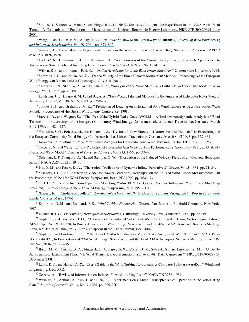
Figure 3. Comparison of the variation of the predicted power coefficient with tip-speed ratio for θtip = 4.

Figure 4. Comparison of the variation of the predicted thrust coefficient with tip-speed ratio for θtip = 4.

achieved for a TSR of around 5.75 from both the BEM theory and the FVM. From the BEM theory results, it isevident that the addition of the tip losses causes significant change in the predicted power output, whereas the additionof the viscous losses does not significantly alter the power output. For the low values of TSR, there is no significantdifference in the predicted power output with and without viscous losses in the FVM calculations. The addition of

10American Institute of Aeronautics and Astronautics

0

0.1

0.2

0.3

0.4

0.5

0.6

0 2 4 6 8 10 12 14

BEM (tip + profile losses)Free Wake (tip + profile losses)

Pow

er c

oeffi

cien

t, C

P

Tip-speed ratio, XTSR

θtip

= 1o, σ = 0.05

Ideal twist

BEM fails

0

0.5

1

1.5

2

2.5

3

0 2 4 6 8 10 12 14

BEM (tip + profile losses)

Free Wake (tip + profile losses)

Thr

ust

coef

ficie

nt, C

T

Tip-speed ratio, XTSR

θtip

= 1o, σ = 0.05

Ideal twist

BEM fails

Figure 5. Comparison of the variation of the predicted power coefficient with tip-speed ratio for θtip = 1.

Figure 6. Comparison of the variation of the predicted thrust coefficient with tip-speed ratio for θtip = 1.

viscous losses, however, reduces the power output at moderate to high values of TSR.The agreement between the predicted power coefficient from the FVM and the BEM theory was noted to be very

good for low values of TSR. As the TSR is increased further, the turbulent wake/vortex ring state is encountered. Here,the BEM theiry fails because the wake induction factor is greater than 0.5. In this region, the power coefficient from

11American Institute of Aeronautics and Astronautics

0

0.3

0.6

0.9

1.2

1.5

0 0.2 0.4 0.6 0.8 1

TSR = 16.667TSR = 13.333TSR = 8.3333TSR = 6.6667TSR = 4.1667TSR = 2.0830

Axi

al in

duct

ion

fact

or, a

Non-dimensional distance, r/R

θt ip

= 1o, σ = 0.05

Ideal twist

(a)

0

0.02

0.04

0.06

0.08

0.1

0.12

0 0.2 0.4 0.6 0.8 1

TSR = 16.667TSR = 13.333TSR = 8.3333TSR = 6.6667TSR = 4.1667TSR = 2.0831

Axi

al in

duct

ion

fact

or, a

'

Non-dimensional distance, r/R

θt ip

= 1o , σ = 0.05

Ideal twist

(b)

Figure 7. FVM wake prediction of the distribution of the induction factors for various tip-speed ratios: (a) axial inductionfactor, (b) tangential induction factor.

12American Institute of Aeronautics and Astronautics

the BEM method using the Glauert correction is shown. The variation of the thrust coefficient (see Fig. 4) with TSR isalmost linear. Again, the BEM method and the FVM predictions are found to be in very good agreement up to a TSRof 6. Beyond this, the BEM theory with tip-losses breaks down and the BEM method with no losses underpredicts thethrust coefficient.

Figure 5 shows the comparison of the power and thrust coefficient, respectively, for θtip = 1 including both thetip losses and profile losses. Hereafter, a lower tip pitch angle (θtip = 1) is used because the modified BEM equationsbreak-down at higher values of TSR. The predicted power coefficient from the FVM and the BEM theory are in goodagreement for XTSR < 5. For higher values of TSR, the BEM calculation with the Glauert correction significantlyunderpredicts the power coefficient. Notice that the predicted thrust coefficient (Fig. 6) from the two methods are verysimilar until the BEM theory breaks down.

Figures 7(a) and (b) show the distribution of the axial and the tangential induction factor over the blade for varioustip-speed ratios, as obtained from the FVM calculation. For higher values of TSR, the average induction factor islarger. It can be seen that the value of the axial induction factor for moderate values of TSR is very large near theblade root and blade tip. This also causes the modified BEM method with the Glauert correction to break-down. Theaverage value of the tangential induction factor [see Fig. 7(b)] decreases with increasing values of TSR. However, thetangential induction factor is noted to be very small compared to the axial induction factor except near the blade root.This justifies neglecting the effect of swirl in the BEM methodology, as assumed previously.

Although the above results show that the integrated thrust and power coefficients obtained from the BEM andFVM calculations are in good agreement for low values of TSR, predicting the local distribution of airloads accuratelyis very important for the reliable design of wind turbines. Figures 8 through 10 compare the local variation of theinduction factor and the thrust and power coefficient for two different cases: (1) Same tip pitch, and (2) Same thrustcoefficient. In the second case, the thrust coefficient obtained from the FVM is prescribed for the BEM calculation.

Figures 8(a) and (b) show the distribution of the induction factor over the blade for the two cases for a TSR of6.0. The BEM result with no tip-losses is also shown. It can be seen that the tip-losses cause an increase in the axialinduction factor near the blade tip and root, which is captured very well in the BEM method using the Prandtl tip-lossfunction. The overall agreement in the local induction factors obtained with the FVM and BEM theory is good whenthe tip pitch is the same for the two calculations, but worsens when the thrust coefficient obtained from the BEMapproach is trimmed to match the thrust from the FVM.

Figures 9 and 10 show the thrust and the power coefficient distributions for the two cases. The thrust coefficientdistribution agrees very well for the second method, whereas the local CT is over-predicted when the tip-pitch is keptthe same in the two calculations. In both cases, the FVM gives a slightly higher local power coefficient as comparedto the BEM theory. These results shows that the integrated power and thrust predicted by the two methods are in goodagreement. However, the predictions of the local induction factor, the thrust coefficient and the power coefficient arenot so similar for the two methods, even for moderate tip-speed ratios.

IV. Wind Turbine in Yawed Flow

Because of the variability of wind direction and the need to yaw the rotor out of the wind to limit power at highwind speeds, wind turbines work in yawed flow for a significant amount of their operational time. BEM methods arefundamentally incapable of handling this problem without the prescription of a modified inflow at the rotor disk.

A FVM calculation has been performed where a turbine yaws 30 out of the wind during the period of 2 revolutions.Figure 11 shows the top view of the evolving wake at different times. Just after the yaw starts, the turbine moves intoits own wake, which can cause highly unsteady loads on the rotor blades. After 5 revolutions, the wake reorganizesand shows disturbances only along the filaments for the last 2 to 3 wake turns. After about 10 revolutions, the wakebecomes essentially periodic. The corresponding time-history of the power output is shown in Fig. 12. Notice thatthe power output drops rapidly with yaw; this drop is proportional to the cube of the yaw angle. After the wake startsreorganizing, there is some recovery in the power output. After 10 revolutions the power output becomes essentiallyperiodic with a strong 2/rev output variation.

To apply the BEM method to a wind turbine in yawed flow, an additional approximation to the inflow throughthe wind turbine rotor is required. Usually, the axial induction factors for the unyawed case are calculated first and acorrection for the yawed flow effects29 based on linear inflow models19–21 is then applied. For a wind turbine operating

13American Institute of Aeronautics and Astronautics

0

0.2

0.4

0.6

0.8

1

0 0.2 0.4 0.6 0.8 1

BEM (without tip-loss)BEM (with tip-loss)Free vortex wake

Axi

al in

duct

ion

fact

or, a

Non-dimensional distance, r/R

(a)

0

0.2

0.4

0.6

0.8

1

0 0.2 0.4 0.6 0.8 1

BEM (without tip-loss)BEM (with tip-loss)Free vortex wake

Axi

al in

duct

ion

fact

or, a

Non-dimensional distance, r/R

(b)

Figure 8. Distribution of the induction factor along the blade for a tip-speed ratio of XTSR = 6.0 and θtip = 1 : (a) Samevalue of θtip, (b) Same value of CT .

14American Institute of Aeronautics and Astronautics

0

0.5

1

1.5

2

0 0.2 0.4 0.6 0.8 1

BEM (without tip-loss)BEM (with tip-loss)Free vortex wake

dCT/d

r

Non-dimensional distance, r/R

(a)

θt ip

= const

0

0.5

1

1.5

2

0 0.2 0.4 0.6 0.8 1

BEM (without tip-loss)BEM (with tip-loss)Free vortex wake

dCT/d

r

Non-dimensional distance, r/R

(b)

CT = const

Figure 9. Distribution of the thrust coefficient along the blade for a tip-speed ratio of XTSR = 6.0 and θtip = 1 : (a) Samevalue of θtip, (b) Same value of CT .

15American Institute of Aeronautics and Astronautics

0

0.3

0.6

0.9

1.2

0 0.2 0.4 0.6 0.8 1

BEM (without tip-loss)BEM (with tip-loss)Free vortex wake

dCP/d

r

Non-dimensional distance, r/R

(a)

θt ip

= const

0

0.3

0.6

0.9

1.2

0 0.2 0.4 0.6 0.8 1

BEM (without tip-loss)BEM (with tip-loss)Free vortex wake

dCP/d

r

Non-dimensional distance, r/R

(b)

CT = const

Figure 10. Distribution of the power coefficient along the blade for a tip-speed ratio of XTSR = 6.0 and θtip = 1 : (a) Samevalue of θtip, (b) Same value of CT .

16American Institute of Aeronautics and Astronautics

-2

-1.5

-1

-0.5

0

0.5

1

1.5

2

-1 0 1 2 3 4 5

La

tera

l d

isp

lace

me

nt,

x/R

Axial displacement, z/R

(a) time = 0

-2

-1.5

-1

-0.5

0

0.5

1

1.5

2

-1 0 1 2 3 4 5

La

tera

l d

isp

lace

me

nt,

x/R

Axial displacement, z/R

(b) time = 2 revs

-2

-1.5

-1

-0.5

0

0.5

1

1.5

2

-1 0 1 2 3 4 5

La

tera

l d

isp

lace

me

nt,

x/R

Axial displacement, z/R

(c) time = 5 revs

-2

-1.5

-1

-0.5

0

0.5

1

1.5

2

-1 0 1 2 3 4 5

La

tera

l d

isp

lace

me

nt,

x/R

Axial displacement, z/R

(d) time = 10 revs

-2

-1.5

-1

-0.5

0

0.5

1

1.5

2

-1 0 1 2 3 4 5

La

tera

l d

isp

lace

me

nt,

x/R

Axial displacement, z/R

(e) time = 20 revs

-2

-1.5

-1

-0.5

0

0.5

1

1.5

2

-1 0 1 2 3 4 5

La

tera

l d

isp

lace

me

nt,

x/R

Axial displacement, z/R

(f) time = 60 revs

Figure 11. Top view of the evolving wake geometry behind the wind turbine yawing 30 out of the wind. (a) Time = 0, (b)Time = 2revs., (c) Time = 5 revs., (d) Time = 10 revs., (e) Time = 20 revs. and (f) Time = 60 revs.

17American Institute of Aeronautics and Astronautics

0

0.1

0.2

0.3

0.4

0.5

0.6

-5 0 5 10 15 20

Pow

er c

oeffi

cien

t, C

P

Revolutions

θtip

= 1o, σ = 0.05

Ideal twist

Turbine yaws

30o out of the wind

Figure 12. Power coefficient as a function of time for when the turbine is yawed 30 out of the wind.

in yawed flow at an angle γ, the inflow can be represented by

a(r,γ) = a(r,γ = 0)+a0(kxr cosψ+ kyr sinψ) (26)

where a0 is the mean axial induction factor given by the momentum theory. The coefficients kx and ky are the lon-gitudinal and lateral inflow weighting factors, respectively, which vary with the linear inflow model being used. Inthis study, a simple Coleman model19 is considered for the comparison with the FVM, which seems to be a commonmodel used in wind turbine applications. In the Coleman model, the weighting factors are given by

kx = tan(χ/2) ky = 0.0 (27)

where χ is the wake skew angle obtained using the momentum theory and is given by

χ = tan−1(

V∞ sinγV∞ cosγ− vi

)(28)

Figure 13(a) shows the distribution of the axial induction factor along the longitudinal axis in the rotor disk planefor different yaw angles as obtained using the FVM method and from the BEM theory with a Coleman inflow cor-rection. The comparison shows that the BEM method with a yawed flow correction gives good agreement with theFVM for smaller yaw angles, whereas the agreement is not as good for the larger yaw angles. The asymmetry in theaxial induction factor across the disk is also not in agreement with the FVM. The distribution of axial induction factorsalong the lateral axis of the rotor is shown in Fig. 13(b). It can be seen that the distribution of a is symmetric overthe rotor for smaller yaw angles. However, for γ = 30 some asymmetry can be observed from the FVM calculation.The BEM predictions with the Coleman correction overlap for different yaw angles because ky = 0, which holds forsmaller yaw angles but is obviously not valid for larger yaw angles.

The above results show that the BEM theory with linear inflow assumption seems to give acceptable agreementwith the FVM calculation, but only for small yaw angles. For larger yaw angles, the agreement between the predictedinduction factor distribution along the longitudinal and lateral axis of the turbine disk from the BEM theory and theFVM is not as good.

18American Institute of Aeronautics and Astronautics

0

0.2

0.4

0.6

0.8

1

-1 -0.5 0 0.5 1

γ = 5o, FVM

γ = 15o, FVM

γ = 30o , FVM

γ = 5o, BEM + Coleman

γ = 15o, BEM + Coleman

γ = 30o, BEM + Coleman

Axi

al in

duct

ion

fact

or, a

Non-dimensional lateral position, x/R

V∞

γθ

t ip= 1o , σ = 0.05

Ideal twist

(a)

0

0.2

0.4

0.6

0.8

1

-1 -0.5 0 0.5 1

γ = 5o , FVM

γ = 15o , FVM

γ = 30o , FVM

γ = 5o, BEM + Coleman

γ = 15o, BEM + Coleman

γ = 30o, BEM + Coleman

Axi

al in

duct

ion

fact

or, a

Non-dimensional longitudinal position, y/R

θt ip

= 1o, σ = 0.05

Ideal twist

(b)

Figure 13. Distribution of the differential axial induction factor along the longitudinal axis in yawed flow with respect tothe unyawed flow.

V. Universal Thrust and Power Coefficient Curve

To understand various flow states of a rotor over which the BEM theory can be applied, it is instructive to constructa universal power and thrust coefficient curve. In helicopter theory, the universal induced velocity curve gives therelation between the axial velocity and the induced velocity at a constant thrust. This relation can be expressed interms of the variation of thrust coefficient with the axial induction factor.

19American Institute of Aeronautics and Astronautics

The axial induction factor for a wind turbine, a, is defined as the ratio of induced velocity at the rotor disk to thefree stream velocity (i.e., a = vi/V∞). This can be expressed in terms of the ratio of induced velocity and inducedvelocity of a powered rotor in hovering flight using

a =vi

V∞=

vi

vh

( vh

V∞

)(29)

where vi/vh is a function of the axial free-stream velocity, V∞. The exact solution for vi/vh in the normal working state(V∞/vh > 0) is given by

vi

vh= − V∞

2vh+

√( V∞

2vh

)2+1 (30)

In the windmill brake state (V∞/vh < −2), the solution is given by

vi

vh= − V∞

2vh−

√( V∞

2vh

)2−1 (31)

For the turbulent wake state/vortex ring state, no exact solution is available from the momentum theory. The relationfor the induced velocity in the range −2 < V∞/vh < 0 has been expressed as a quartic fit by Leishman25 based onexperimental measurements for helicopter rotors as given by Gessow in Ref. 30. This relation can be used to expressthe axial induction factor in terms of V∞/vh using Eq. 29, i.e.,

vi

vh= A+B

V∞

vh+C

(V∞

vh

)2+D

(V∞

vh

)3+E

(V∞

vh

)4(32)

where A = 1.15, B = −1.125, C = −1.372, D = −1.718 and E = −0.665. The thrust coefficient for a helicopter isdefined as

CThel =T

ρA(ΩR)2 (33)

This form of the thrust coefficient can be expressed in terms of the mean inflow as

CThel = 2λ2h (34)

where λh = vh/ΩR. Here vh is the induced velocity at the rotor disk in hover. The thrust coefficient for a wind turbineis defined as

CTwt =T

12 ρAV 2

∞(35)

which can be reexpressed in terms of the helicopter thrust coefficient as

CTwt = 2CThel

(ΩRV∞

)2= 4

(V∞

vh

)−2(36)

In a similar manner, the power coefficient for wind turbine is defined as

CPwt =P

12 ρAV 3

∞= CTwt(1−a) (37)

The value of CPwt can now be expressed in terms of the ratio V∞/vh using the expressions for CTwt and a in terms ofV∞/vh.

For a given V∞/vh, the thrust coefficient and the axial induction factor can be obtained and these are plotted inFig. 14. The solid line shows the momentum theory predictions in the windmill brake state. The momentum theoryfails when the axial induction factor is greater than 0.5. Various empirical corrections have been suggested for thisrange some of which are shown in Fig. 14(a). The Glauert fit for the thrust coefficient for a > 0.5 is given by

CT = 4a(a−1)+2 (38)

20American Institute of Aeronautics and Astronautics

0

5

10

15

20

0 0.5 1 1.5 2 2.5 3

BEM (a < 0.5) BEM (a > 0.5) Glauert fit Leishman fit Climb Washizu et. al Lock

Thr

ust

coef

ficie

nt,

CT

Axial induction factor, a

(a)

To hover

From hover

VRSWBS

NWS

TWS

0.01

0.1

1

10

100

1000

0.01 0.1 1 10 100

BEM (a < 0.5) BEM (a > 0.5) Glauert fit Leishman fit Climb Washizu et. al Lock

Thr

ust

coef

ficie

nt,

CT

Axial induction factor, a

(b)

To hoverFrom hover

NWSVRS

WBS

TWS

Figure 14. Variation of the thrust coefficient with the axial induction factor for normal working state (NWS), turbulentwake state (TWS), vortex ring state (VRS) and windmill brake state (WBS): (a) Linear scale and (b) Log scale to show theasymptotic values.

21American Institute of Aeronautics and Astronautics

-4

-2

0

2

4

0 0.5 1 1.5 2

BEM (a < 0.5) BEM (a > 0.5) Climb Leishman fit

Pow

er c

oeffi

cien

t, C

P

Axial induction factor, a

(a)

To hover

From hover

WBS

VRS

BEMT fails

NWSTWS

-10

-8

-6

-4

-2

0

2

4

0.01 0.1 1 10

BEM (a < 0.5) BEM (a > 0.5) Climb Leishman fit

Pow

er c

oeffi

cien

t, C

P

Axial induction factor, a

(b)

To hover

VRS

WBS

From hover

NWS

TWS

Figure 15. Variation of the power coefficient with the axial induction factor for normal working state (NWS), turbulentwake state (TWS), vortex ring state (VRS) and windmill brake state (WBS): (a) Linear scale and (b) Log scale to show theasymptotic values.

22American Institute of Aeronautics and Astronautics

Experimental measurements in this flow state from Lock9 and Washizu et al.31 are also shown. As the descent velocitythrough the rotor decreases and the hovering state is approached, the thrust coefficient and the axial induction factorapproach infinity, which indicates the asymptotic limits shown in Fig. 14(b). This corresponds to the VRS where thevortex filaments are bundled up near the rotor disk. In the second branch, the climb velocity is increased from hoverand the variation of the thrust coefficient with the axial induction factor is shown. As the climb velocity is increased,the thrust coefficient approaches zero.

The variation of the power coefficient with the axial induction factor for the various flow states is shown inFig. 15(a). The power coefficient, CP is defined as positive when the rotor is extracting power from the wind. Themomentum theory is valid until a = 0.5. An approximate fit for the CP variation (Leishman fit) is also shown in thisfigure. Again, when powered hovering flight is approached the value of the power coefficient and the axial inductionfactor approaches infinity, as shown in Fig. 15(b). The above results show that the Glauert correction was really ob-tained only for a limited set of experimental values. The agreement between the extended set of experimental resultsand Glauert correction in the vortex ring state is not as good, whereas the Leishman fit shows a good agreement forthe whole range of axial induction factors.

VI. Conclusions

A comparison of the thrust and power output based on blade-element momentum theory (BEM) and free-vortexmodel (FVM) has been performed. The following conclusions have been drawn from the work:

1. Good agreement in the power and thrust prediction is observed between the FVM and BEM methods for lowtip-speed ratios (XTSR < 6). For higher tip-speed ratios, the wake induction factor is very high near the tip regionand the BEM model fails. It is also shown that the corrections for CT at higher axial induction factors maybreak-down. On the other hand, the FVM shows the flexibility for the aerodynamic analysis of wind turbines inall working states including the vortex ring state (high TSR).

2. The FVM can also be used for the aerodynamic analysis of wind turbines in yawed flow for which BEM methodis less applicable without resorting to various types of approximations. It is also shown that the linear inflowmodels often used with the BEM theory are probably not applicable for large yaw angles. The ability of theFVM to capture the time accurate behavior of the aerodynamic response of wind turbine in yawed flow has alsobeen shown.

3. A universal thrust and power coefficient curve has been derived to understand various flow states of a windturbine (i.e., normal working state, turbulent wake state and the windmill brake state). In the vortex ring state,the Glauert correction is shown to be adequate only when the axial induction factor is between 0.5 and 1.

Acknowledgements

This work has been supported by National Renewable Energy Laboratory (NREL) in Golden Colorado. Dr. ScottSchreck was the technical monitor.

References

1Vermeer, L. J., Sørenson, J. N. and Crespo, A., “Wind Turbine Wake Aerodynamics,” Progress in Aerospace Sciences, Vol.39, 2003, pp. 467–510.

2Leishman, J. G., “Challenges in Modeling the Unsteady Aerodynamics of Wind Turbines,” Wind Energy, Vol. 5, 2002,pp. 86–132.

3Snel, H., “Review of the Wind Turbine Aerodynamics,” Wind Energy, Vol. 6, No. 3, July/September, 2003, pp. 203–211.4Hansen, A. C. and Butterfield, C. P., “Aerodynamics of Horizontal-Axis Wind Turbines,” Annual Review of Fluid Mechanics,

Vol. 25, 1993, pp. 115–149.5Fingersh, L. J., Simms, D., Hand, M., Jager, D., Cotrell, J., Robinson, M., Schreck, S. and Larwood, S. “Wind Tunnel Testing

of NREL’s Unsteady Aerodynamics Experiment,” AIAA Paper 2001–0035, 39th Aerospace Sciences Meeting, Reno, NV, Jan. 8–11, 2001.

23American Institute of Aeronautics and Astronautics

6Simms, D., Schreck, S., Hand, M. and Fingersh, L. J., “NREL Unsteady Aerodynamics Experiment in the NASA-Ames WindTunnel: A Comparison of Predictions to Measurements,” National Renewable Energy Laboratory, NREL/TP-500-29494, June2001.

7Wang, T., and Coton, F. N., “A High Resolution Tower Shadow Model for Downwind Turbines,” Journal of Wind Engineeringand Industrial Aerodynamics, Vol. 89, 2001, pp. 873–892.

8Glauert, H. “The Analysis of Experimental Results in the Windmill Brake and Vortex Ring States of an Airscrew,” ARC R& M, No. 1026, 1926.

9Lock, C. N. H., Bateman, H., and Townsend, H., “An Extension of the Vortex Theory of Airscrews with Applications toAirscrews of Small Pitch and Including Experimental Results,” ARC R & M, No. 1014, 1926.

10Wilson, R E., and Lissaman, P. B. S., “Applied Aerodynamics of the Wind Power Machines,” Oregon State University, 1974.11Sørenson, J. N., and Mikkelsen, R., “On the Validity of the Blade Element Momentum Method,” Proceedings of the European

Wind Energy Conference held at Copenhagen, July 2–6, 2001.12Sørenson, J. N., Shen, W. Z., and Munduate, X., “Analysis of the Wake States by a Full-Field Actuator Disc Model,” Wind

Energy, Vol. 1, 1998, pp. 73–88.13Leishman, J. G., Bhagwat, M. J., and Bagai, A., “Free-Vortex Filament Methods for the Analysis of Helicopter Rotor Wakes,”

Journal of Aircraft, Vol. 39, No. 5, 2003, pp. 759–775.14Simoes, F. J., and Graham, J. M. R., “ Prediction of Loading on a Horizontal Axis Wind Turbine using a Free Vortex Wake

Model,” Proceedings of the British Wind Energy Conference, 1991.15Bareiss, R., and Wagner, S., “The Free Wake/Hybrid Wake Code RVOLM – A Tool for Aerodynamic Analysis of Wind

Turbines,” In Proceedings of the European Community Wind Energy Conference held at Lubeck-Travemunde, Germany, March8–12 1993, pp. 424–427.

16Voutsinas, S. G., Belessis, M., and Huberson, S., “Dynamic Inflow Effects and Vortex Particle Methods,” In Proceedings ofthe European Community Wind Energy Conference held at Lubeck-Travemunde, Germany, March 8–12 1993, pp. 428–431.

17Korcurek, D., “Lifting Surface Performance Analysis for Horizontal Axis Wind Turbines,” SER/STR-217-3163, 1987.18Coton, F. N., and Wang, T., “The Prediction of Horizontal Axis Wind Turbine Performance in Yawed Flow Using an Unsteady

Prescribed Wake Model,” Journal of Power and Energy, Vol. 213, 1999, pp. 33–43.19Coleman, R. P., Fiengold, A. M., and Stempin, C. W., “Evaluation of the Induced Velocity Fields of an Idealized Helicopter

Rotor,” NACA ARR L5E10, 1945.20Pitt, D. M., and Peters, D. A., “Theoretical Predictions of Dynamic Inflow Derivatives,” Vertica, Vol. 5, 1981, pp. 21–34.21Schepers, J. G., “An Engineering Model for Yawed Conditions, Developed on the Basis of Wind Tunnel Measurements,” In

the Proceedings of the 18th Wind Energy Symposium, Reno, NV, 1999, pp. 164–174.22Snel, H., “Survey of Induction Dynamics Modelling Within BEM like Codes: Dynamic Inflow and Yawed Flow Modelling

Revisited,” In Proceedings of the 20th Wind Energy Symposium, Reno, NV, 2001.23Glauert, H., “Airplane Propellers,” Aerodynamic Theory, ed. W. F. Durand, Springer-Verlag, 1935. (Reprinted by Peter

Smith, Glouster, Mass., 1976)24Eggleston, D. M., and Stoddard, F. S., Wind Turbine Engineering Design, Van Nostrand Reinhold Company, New York,

1987.25Leishman, J. G., Principles of Helicopter Aerodynamics, Cambridge University Press, Chapter 2, 2000, pp. 58–59.26Gupta, S., and Leishman, J. G., “Accuracy of the Induced Velocity of Wind Turbine Wakes Using Vortex Segmentation,”

AIAA Paper No. 2004-0828, In Proceedings of 23rd Wind Energy Symposium and the 42nd AIAA Aerospace Sciences Meeting,Reno, NV, Jan. 5–8, 2004, pp. 339–353. To appear in the AIAA Journal, Dec. 2004.

27Gupta, S., and Leishman, J. G., “Stability of Methods in the Free-Vortex Wake Analysis of Wind Turbines,” AIAA PaperNo. 2004-0827, In Proceedings of 23rd Wind Energy Symposium and the 42nd AIAA Aerospace Sciences Meeting, Reno, NV,Jan. 5–8, 2004, pp. 339–353.

28Hand, M. M., Simms, D. A., Fingersh, L. J., Jager, D. W., Cortell, J. R., Schreck, S., and Larwood, S. M., “UnsteadyAerodynamics Experiment Phase VI: Wind Tunnel test Configurations and Available Data Campaigns,” NREL/TP-500-29955,December 2001.

29Laino, D. J., and Hansen A. C., “User’s Guide to the Wind Turbine Aerodynamics Computer Software AeroDyn,” WindwardEngineering, Dec. 2002.

30Gessow, A., “Review of Information on Induced Flow of a Lifting Rotor,” NACA TN 3238, 1954.31Washizu, K., Azuma, A., Koo, J., and Oka, T., “Experiments on a Model Helicopter Rotor Operating in the Vortex Ring

State,” Journal of Aircraft, Vol. 3, No. 3, 1966, pp. 225–230.

24American Institute of Aeronautics and Astronautics