
different strategies to obtain antimicrobial biodegradable films ...
Upload
khangminh22Category
view
0download
0
Res Electricae Magdeburgenses
Magdeburger Forum zur Elektrotechnik
Comparison of Different Redispatch Optimiza-
tion Strategies
Iryna Chychykina
MAFO
Band 78

Res Electricae Magdeburgenses
Magdeburger Forum zur Elektrotechnik, Jg. 7, Band 78, 2019
http://www.mafo.ovgu.de/
IMPRESSUM
Herausgeber:
Prof. Dr.-Ing. Andreas Lindemann, Lehrstuhl für Leistungselektronik, Institut
für Elektrische Energiesysteme
Prof. Dr.-Ing. habil. Martin Wolter, Lehrstuhl für Elektrische Netze und Erneu-
erbare Energie, Institut für Elektrische Energiesysteme
Prof. Dr. rer. nat. Georg Rose, Lehrstuhl für Medizinische Telematik/Medizin-
technik, Institut für Medizintechnik
Prof. Dr.-Ing. Ralf Vick, Lehrstuhl für Elektromagnetische Verträglichkeit, Insti-
tut für Medizintechnik
Gründungsherausgeber:
Prof. Dr. rer. nat. habil. Jürgen Nitsch
Prof. Dr.-Ing. habil. Zbigniew Antoni Styczynski
alle: Otto-von-Guericke-Universität Magdeburg
Postfach 4120, 39016 Magdeburg
V. i. S. d. P.:
Dr.-Ing. Iryna Chychykina
Otto-von-Guericke-Universität Magdeburg, Postfach 4120, 39016 Magdeburg
1. Auflage, Magdeburg, Otto-von-Guericke-Universität, 2019
Zugl.: Magdeburg, Univ., Diss., 2019
Auflage: 50
Redaktionsschluss: Dezember 2019
ISSN: 1612-2526
ISBN: 978-3-944722-xx-y
© Copyright 2019 Iryna Chychykina
Bezug über die Herausgeber
Druck: docupoint GmbH
Otto-von-Guericke-Allee 14, 39179 Barleben

Comparison of Different Redispatch Optimiza-
tion Strategies
Dissertation
zur Erlangung des akademischen Grades
Doktoringenieurin
(Dr.-Ing.)
von M.Sc. Iryna Chychykina
geb. am 15.06.1988 in Antrazyt (Ukraine)
genehmigt durch die Fakultät für Elektrotechnik und Informationstechnik der Otto-von-
Guericke-Universität Magdeburg
Gutachter:
Prof. Dr.-Ing. habil. Martin Wolter
Prof. Dr.-Ing. Dirk Westermann
Promotionskolloquium am 18 November 2019

I
I Abstract
In the recent years, line congestions in the electric transmission networks occur quite fre-
quently due to the power grids were not originally designed for the current amount of
energy and its strong fluctuation. Furthermore, the increasing utilization of renewable
distributed energy sources, growth of the network complexity, reduction of the conven-
tional power plant utilization, forecast errors and strong electricity market competition
frequently bring the power grids to their transmission limits as well. Therefore, the risk
of congestions has permanently increased, especially in central Europe.
If a line congestion occurs in the electric network, the transmission system operator has
to apply a suitable remedial action to overcome the problem as fast as possible, e.g by
utilization of redispatch, which is very common in Germany. However, this measure can
cause high costs for the transmission network operators. For this reason, the realization
of an economically efficient and optimal redispatching has become very important issue
in the power system operation.
The main goal of this work is a consideration and development of various possibilities
and methods for realization of a technically sound and cost-efficient redispatch in case of
network congestions. Therefore, different numerical and metaheuristic optimization tech-
niques are implemented, compared with respect to their complexity, efficiency, reliabil-
ity, simulation time etc. and verified through a small test grid and simplified ENTSO-E
network model.
Furthermore, it is shown which technical and economic aspects of redispatching have a
major influence on its realization and should always be taken into account or can be ne-
glected while solving the redispatch optimization problem. Here, different approaches of
the network sensitivity analysis are evaluated and compared as well.
Finally, the transmission network operators can use the knowledge and results of this
work to improve the current redispatch realization in their power grids, and thus to reduce
the redispatch costs, which are especially high in Germany.

II
II Kurzfassung
In den letzten Jahren hat die Häufigkeit des Auftretens von Engpässen in den elektrischen
Übertragungsnetzen stark zugenommen, weil die Stromnetze ursprünglich für die aktu-
elle Energiemenge und deren starke Schwankung nicht ausgelegt sind. Darüber hinaus
bringen die weiter steigende Nutzung der erneuerbaren dezentralen Energiequellen, die
zunehmende Netzkomplexität, die Abschaltung konventioneller Kraftwerke, Progno-
sefehler und der starke Wettbewerb auf dem Strommarkt die elektrischen Netze immer
öfter an ihre Übertragungsgrenzen. Daher ist die Gefahr von Engpässen permanent ge-
stiegen, insbesondere in Mitteleuropa.
Wenn ein Engpass im Stromnetz entstanden ist, sind die Übertragungsnetzbetreiber ver-
pflichtet, eine geeignete Abhilfemaßnahme so schnell wie möglich anzuwenden, um ihn
zu beseitigen, z. B. durch den deutschlandweit verbreiteten Redispatch. Allerdings kann
diese Gegenmaßnahme hohe Kosten für die Übertragungsnetzbetreiber verursachen, die
zum Schluss die Stromverbraucher zahlen müssen. Deswegen ist die Realisierung eines
kosten- und technisch effizienten Redispatches ein sehr wichtiges Thema des Netzbe-
triebs geworden.
Daher ist das Hauptziel dieser Arbeit, unterschiedliche Möglichkeiten und Ansätze für
eine kostengünstige Redispatchumsetzung bei Entstehung der Engpässe zu entwickeln.
Dafür werden verschiedene numerische und metaheuristische Optimierungsmethoden
hinsichtlich ihrer Komplexität, Effizienz, Verlässlichkeit, Detaillierung und Rechenzeit
verglichen und durch ein kleines Netzmodell sowie durch ein vereinfachtes ENTSO-E-
Netzmodell verifiziert.
Schließlich werden die Übertragungsnetzbetreiber durch die Erkenntnisse in dieser Arbeit
in die Lage versetzt, ihre Stromnetze effizienter zu betreiben, in dem der Redispatchpro-
zess verbessert wird. Dabei werden die hohen Redispatchkosten, insbesondere in
Deutschland, deutlich gesenkt.

III
III Table of Contents
I Abstract .............................................................................................................. I
II Kurzfassung ..................................................................................................... II
III Table of Contents............................................................................................ III
IV List of Figures ................................................................................................. VI
V List of Tables ................................................................................................. VII
VI List of Symbols............................................................................................. VIII
VII List of abbreviations ....................................................................................... XI
1 Introduction ...................................................................................................... 1
1.1 Motivation .......................................................................................................... 1
1.2 Objectives ........................................................................................................... 1
1.3 Structure of this work ......................................................................................... 2
2 Congestion management .................................................................................. 4
2.1 Congestions in the power systems...................................................................... 4
2.2 Definition of congestion management ............................................................... 5
2.2.1 Regulation of the congestion management in Europa ........................................ 5
2.2.2 Regulation of the congestion management in Germany .................................... 5
2.3 Congestion management methods ...................................................................... 6
2.3.1 Congestion prevention or remedy (short-term CM) ........................................... 7
2.3.1.1 Redispatch (power generation management) ..................................................... 8
2.3.1.2 Countertrading .................................................................................................... 9
2.3.2 Transmission capacity allocation (long-term CM) ........................................... 10
2.3.2.1 Transmission capacity auctions (market-based) ............................................... 10
2.3.2.2 Administrative procedures ............................................................................... 12
2.3.2.3 Power infeed auctions ...................................................................................... 13
3 Technical and economic aspects of redispatch ............................................ 14
3.1 Technical aspects of redispatch ........................................................................ 14
3.1.1 Redispatch principle ......................................................................................... 14
3.1.2 Sensitivity analysis ........................................................................................... 16
3.1.3 Comparison ...................................................................................................... 20
3.1.3.1 ‘5 Bus’ IEEE power grid model ....................................................................... 20
3.1.3.2 Simplified grid model of the ENTSO-E area ................................................... 24
3.1.3.3 Conclusions ...................................................................................................... 26
3.2 Economic aspects of redispatch ....................................................................... 27
3.2.1 Levelized costs of electricity ............................................................................ 27
3.2.2 Power plant cycling costs ................................................................................. 27

III Table of Contents IV
3.2.3 Shut-down costs ............................................................................................... 31
4 Optimization methods .................................................................................... 32
4.1 Linear programming ......................................................................................... 32
4.1.1 Simplex algorithm ............................................................................................ 33
4.1.1.1 General approach .............................................................................................. 34
4.1.1.2 Performance...................................................................................................... 34
4.1.2 Linear redispatch optimization ......................................................................... 35
4.1.2.1 Objective function of the redispatch optimization problem ............................. 35
4.1.2.2 Constraints of the redispatch optimization problem......................................... 36
4.1.3 Sequential simplex ........................................................................................... 37
4.1.3.1 General approach .............................................................................................. 37
4.1.3.2 Algorithm adaptation for the non-linear redispatch optimization problem ...... 39
4.2 Genetic algorithm ............................................................................................. 40
4.2.1 Evolutionary optimization algorithms .............................................................. 40
4.2.2 General approach .............................................................................................. 41
4.2.2.1 Recombination.................................................................................................. 42
4.2.2.2 Mutation ........................................................................................................... 44
4.2.2.3 Selection ........................................................................................................... 44
4.2.3 Constraint handling .......................................................................................... 45
4.2.3.1 Death penalty .................................................................................................... 46
4.2.3.2 Static penalty .................................................................................................... 46
4.2.3.3 Dynamic Penalty .............................................................................................. 47
4.2.4 Performance...................................................................................................... 47
4.2.5 Non-linear redispatch optimization problem for the GA ................................. 48
4.2.6 Algorithm adaptation for the non-linear redispatch optimization problem ...... 49
4.3 Mean Variance Mapping Optimization ............................................................ 51
4.3.1 General approach .............................................................................................. 51
4.3.2 Performance...................................................................................................... 55
4.3.3 Non-linear redispatch optimization problem for the MVMO .......................... 55
4.3.4 Algorithm adaptation for the non-linear redispatch optimization problem ...... 56
4.4 Particle Swarm Optimization ........................................................................... 57
4.4.1 General approach .............................................................................................. 57
4.4.1.1 Inertia weight factor ......................................................................................... 59
4.4.1.2 Recommended parameter values ...................................................................... 60
4.4.2 Performance...................................................................................................... 60
4.4.3 Non-linear redispatch optimization problem for the PSO ................................ 61
4.4.4 Algorithm adaptation for the non-linear redispatch optimization problem ...... 61
4.5 Ant Colony Optimization ................................................................................. 62

III Table of Contents V
4.5.1 General approach .............................................................................................. 62
4.5.1.1 Ant Colony Optimization algorithm for continuous domain ........................... 65
4.5.1.2 Ant Colony Optimization algorithm with the Prospect Theory for continuous
domain .............................................................................................................. 67
4.5.2 Performance...................................................................................................... 69
4.5.3 Non-linear redispatch optimization problem for the ACO ............................... 69
4.5.4 Algorithm adaptation for the non-linear redispatch optimization problem ...... 69
5 Case study ....................................................................................................... 71
5.1 Test network models ........................................................................................ 71
5.1.1 Small network model........................................................................................ 71
5.1.2 Simplified ENTSO-E network model .............................................................. 72
5.2 Redispatch optimization without considering the power plant cycling costs .. 75
5.2.1 Simulation results in the small network model ................................................ 75
5.2.1.1 Single network line congestion ........................................................................ 75
5.2.1.2 Multiple network line congestion ..................................................................... 77
5.2.2 Simulation results in the simplified ENTSO-E network model ....................... 79
5.2.2.1 Multiple network line congestion ..................................................................... 79
5.3 Redispatch optimization considering the power plant cycling costs ................ 82
5.3.1 Simulation results in the small network model ................................................ 82
5.3.2 Simulation results in the simplified ENTSO-E network model ....................... 85
5.3.3 Conclusions ...................................................................................................... 87
6 Summary and Outlook ................................................................................... 89
7 List of references ............................................................................................ 91
A Title Annex A .................................................................................................. 99
Published MaFo Books ............................................................................................... 100
VI
IV List of Figures
Figure 2.1 Simplified representation of the CM [11] ............................................ 6
Figure 2.2 Overview of the congestion management classification [8], [12], [13],
[14] ....................................................................................................... 7
Figure 3.1 Redispatch principle ........................................................................... 15
Figure 3.2 ‘5 Bus’ IEEE power grid model ......................................................... 21
Figure 3.3 I-P characteristics for the line ‘L1’ in the ‘5 Bus’ IEEE test network
model .................................................................................................. 22
Figure 3.4 I-P characteristics for the line ‘L1’ in the ‘5 Bus’ IEEE test network
model (zoomed representation) .......................................................... 22
Figure 3.5 I-P characteristics for the line ‘L3’ in the ‘5 Bus’ IEEE test network
model .................................................................................................. 23
Figure 3.6 I-P characteristics for the line ‘L3’ in the ‘5 Bus’ IEEE test network
model (zoomed representation) .......................................................... 24
Figure 3.7 I-P characteristics for the line power line between bus bars ‘1’ and ‘2’
............................................................................................................ 25
Figure 3.8 I-P characteristics for the line power line between bus bars ‘11’ and ‘19’
............................................................................................................ 26
Figure 3.9 Indirect start-up cost function [41] ..................................................... 29
Figure 4.1 Flowchart of the genetic algorithm .................................................... 42
Figure 4.2 Mapping function example [69] ........................................................ 52
Figure 4.3 Algorithm for the determination of the shape variables .................... 54
Figure 4.4 Particle movement .............................................................................. 58
Figure 4.5 Flowchart of particle swarm optimization ......................................... 59
Figure 4.6 Food searching of an ant colony [88], [89], [92] ............................... 63
Figure 4.7 Value function [92] ............................................................................ 67
Figure 5.1 Small test network model ................................................................... 72
Figure 5.2 Cluster model of the e-Highway2050 project [99] ............................ 73
Figure 5.3 Simplified ENTSO-E network model [98] ........................................ 74
Figure 5.4 Bus bar model [98] ............................................................................. 74

VII
V List of Tables
Table 3.1 LCOE for different conventional power plant types [34] .................. 27
Table 3.2 Cycling costs for different conventional power plant types [36] ....... 29
Table 3.3 Indirect cycling costs for different conventional power plant types [36]
............................................................................................................ 30
Table 3.4 PPSDC for different conventional power plant types [45] ................ 31
Table 5.1 Average cost scenario and sensitivity coefficients of lines ‘L2’ and ‘L5’
............................................................................................................ 72
Table 5.2 Simulation results for the single congestion of 346.5 MW on line ‘L5’
taking into account only the linear constraints ................................... 76
Table 5.3 Simulation results for the single congestion of 346.5 MW on line ‘L5’
taking into account the non-linear load flow function ....................... 77
Table 5.4 Simulation results for the multiple congestion on lines ‘L5’ and ‘L7’
taking into account only the linear constraints ................................... 78
Table 5.5 Simulation results for the multiple congestion on lines ‘L5’ and ‘L7’
taking into account the non-linear load flow function ....................... 79
Table 5.6 Positive and negative redispatch potentials in Germany .................... 80
Table 5.7 Average cost scenario ........................................................................ 80
Table 5.8 Simulation results for the multiple congestion on line between bus bars
‘1’ and ‘2’, ‘1’ and ‘3’, ‘11’ and ‘19’ taking into account only the linear
constraints .......................................................................................... 81
Table 5.9 Simulation results for the multiple congestion between bus bars ‘1’ and
‘2’, ‘1’ and ‘3’, ‘11’ and ‘19’ taking into account non-linear load flow
function .............................................................................................. 82
Table 5.10 Special cost scenario of the LCOE and PPCC ................................... 83
Table 5.11 Simulation results for the single congestion of 30 MW on line ‘L5’
taking into account the sensitivity analysis and PPCC ...................... 84
Table 5.12 Simulation results for the single congestion of 30 MW on line ‘L5’
taking into account the non-linear power flow equations and PPCC . 85
Table 5.13 Start-up costs for the scenario in the simplified ENTSO-E network
model .................................................................................................. 86
Table 5.14 Simulation results for the single congestion of 20 MW on the power
line between the bus bars ‘1’ and ‘2’ taking into account the non-linear
power flow equations and PPCC ........................................................ 87
Table 7.1 Sensitivity coefficients of power lines between bus bars ‘1’ and ‘3’, ‘11’
and ‘19’ .............................................................................................. 99

VIII
VI List of Symbols
Notation
A matrix
a vector
a, A scalar
a, A, a, A complex value
Latin symbols
A constraint system
a pivot element
b constraint restrictions
d binary value, distance, parameter of the GA
C penalty coefficient
c acceleration coefficients, costs, chromosome, objective function
F feasible area
f factor, function
G Gaussian, number of power plants
h h-function
I current, identity matrix
J feasible solution, Jacobian
K topological matrix
L route length
P active power
p position, probability
penalty penalty
Q reactive power, optional weighting
q parameter of solution selection
R route
S apparent power
s shape variable
sd binary variable for shut-down
su binary variable for start-up
T simplex tableau

VI List of Symbols IX
t time
U voltage
U unit vector
V probabilistic prospect
v value function, vareance, velocity
w inertia weight factor
x searched variable
Y admittance
Greek symbols
α user-defined constant
β user-defined constant, random number
γ weighting parameter
Δ change
Δτ pheromone quantity
δ phase angle
η heuristic value
λ constant, heat-loss coefficient, user-defined constant
μ mean
ξ factor
ρ pheromone evaporation
σ sensitivity matrix coefficient, standard deviation of the Gaussian distri-
bution function, variance
τ pheromone trail
ω weighting vector
Indexes
best best
c centroid, column number
cong congestion
contr contraction
crp crossover point
dir direct
e expansion

VI List of Symbols X
f ‘father’
fo forced outage
h highest
hr heat rate
incr increase
indr indirect
K node
k exponent, number of solutions
G generator
gl global best position
L line, load
lb current best position
l level number, lowest
LCOE levelized costs of electricity
m ‘mother’, number of constraints
max maximum
min minimum
mut mutation
n number of ants, best solutions, chromosomes, function variables
new new
offspr offspring
old old
RP+, RP- positive and negative redispatch potential
r reflection, row number
ramp ramping
red reduction
s shape
sd shut-down
start smallest value
su start-up
T terminal
Superscript indices
* complex conjugated
T transposed

XI
VII List of abbreviations
ACO Ant Colony Optimization
ACOR-PT Ant Colony Optimization with the Prospect Theory
AC-PTDF AC Power Transfer Distribution Factors
CM Congestion Management
ENTSO-E European Network of Transmission System Operator
GA Genetic Algorithm
LCOE Levelized Costs of Electricity
LP Linear Programming
MF Mapping Function
MVMO Mean Variance Mapping Optimization
PDF Probability Density Function
PFD Power Flow Decomposition method
PPCC Power Plant Cycling Costs
PPSDC Power Plant Shut-Down Costs
PSO Particle Swarm Optimization
PT Prospect Theory
RES Renewable Energy Sources
SS Sequential Simplex
TSO Transmission System Operator
TSP Traveling Salesman Problem

1
1 Introduction
1.1 Motivation
Nowadays, the European electric network very often works at its transmission limits be-
cause of a massive growth of the power system operation complexity and transmission
distances since the end of the nineties, which is caused by the enormous increase of the
European electricity market. These strong changes in the electricity market have occurred
because of the market liberalization, installation of a new European cross-border market
and growing utilization of the renewables. Hence, a limitation of the transmission capac-
ity in the European countries, the permanent increase of the electricity consumption, some
forecast errors and delays in the network expansion can lead to different emergencies
such as network congestions. Therefore, in the recent years, line congestions occur quite
frequently in the European electric transmission network. [1], [2], [3]
In case of a line congestion, the transmission system operators must apply a suitable re-
medial measure as soon as possible. One of the methods to avoid or remedy line conges-
tions is redispatch. It is often used by system operators, especially in central Europe. To-
day, remedial actions of more than several thousand megawatts are a daily routine. Fur-
thermore, there is an increasing risk of complete exhaustion of the redispatch potentials
leading to emergency situations. Therefore, the realization of an efficient redispatch has
become an important topic in the system operation.
Redispatching is a market-related remedial measure. Hence, for an optimal redispatch not
only its technical but also economic aspects, e.g. the power flow equations, network sen-
sitivity analysis, power plant potentials, costs for the redispatch realization, start-up and
shut-down costs of the power plants, should be considered.
1.2 Objectives
In this work, different possibilities and approaches of the redispatch optimization are in-
troduced and verified in test network models. For each developed optimization method,
a suitable formulation of the considered optimization problem is proposed. Here, various
technical and economic aspects of the redispatch realization are taken into account. It is
determined, which components have a strong influence on the redispatching and should

1 Introduction 2
be considered in the optimization problem. Therefore, the introduced optimization prob-
lem consists of different linear and non-linear equations, which make an implementation
of the optimization methods complicated.
Furthermore, the simulation results of the developed optimization approaches for an effi-
cient redispatch realization are compared with regard to the complexity, detailing, relia-
bility, efficiency and computation time.
Finally, the knowledge of this work can help the transmission network operators to realize
the redispatching, resp. to operate their power grids, more efficient. Hence, the costs for
the redispatch can be significantly reduced, which reduces electricity prices for the end
customers.
1.3 Structure of this work
To achieve the above-described objectives, this work is structured as follows.
In chapter 2, processes of congestion management are described in detail. This chapter
gives an overview of a definition of congestion management, its regulations in the Euro-
pean electricity market and the existing congestion management methods.
In chapter 3, different technical and economic aspects of the redispatch realization are
described in detail. Moreover, the Power Flow Decomposition and two AC Power Trans-
fer Distribution Factors methods for the calculation of the network sensitivity analysis
are compared and tested in some standard IEEE and simplified ENTSO-E power grid
models.
In chapter 4, fundamental knowledge of the optimization methods, linear programming
and metaheuristic optimization techniques are provided. Furthermore, the optimization
algorithms, which are used in this work, namely simplex, genetic algorithm, Mean Vari-
ance Mapping Optimization, Particle Swarm Optimization, Ant Colony Optimization, and
different methods for the constraint handling are described in detail. In addition, the per-
formance of the utilized optimization methodologies is introduced.

1 Introduction 3
In chapter 5, the efficiency, accuracy and possible benefits of the previously introduced
metaheuristic algorithms for solving the non-linear redispatch optimization problem are
verified by using different electric network models.
Finally, this work ends with a summary and outlook for a possible future improvement of the
redispatch optimization.

4
2 Congestion management
Since the end of the nineties, there is a drastic growth of the European electricity market
because of the high intensity of market liberalization, newly installed European cross-
border markets and growing use of the renewables. For this reason, the power system
operation complexity and transmission distances rapidly increase as well. The annual load
raise, limitation of the transmission capacity on country borders and general transmission
capacity of the European countries as well as delays in the power grid expansion can lead
to emergency situations of network transmission facilities in different places. Conse-
quently, the risk of network congestions is permanently growing [1]. In addition, in the
future a secure network operation will be more important than a cost reduction for elec-
tricity consumers, because dependence of the industry, public institutions and other con-
sumers on the secure network operation has significantly increased due to the trend to
automation and computerization [2]. Therefore, the network congestion management has
become a very important issue for the transmission network operation.
2.1 Congestions in the power systems
According to the Regulation No 714/2009 of the European Parliament and of the Council
of 13 July 2009 on conditions for an access to network for cross-border exchanges in
electricity, a network congestion means „a situation, in which an interconnection linking
national transmission networks, cannot accommodate all physical flows resulting from
international trade requested by market participants, because of a lack of capacity of the
interconnectors and/or the national transmission systems concerned“. Therefore, the
main reason why congestions occur in the electric networks is a lack of the transmission
capacity [3].
Based on the Continental Europe Operation Handbook of the European Network of the
Transmission System Operators (ENTSO-E), the power system, which consists of n com-
ponents, has to stay stable after a contingency or operational trip of electrical equipment
even with n-1 components. Furthermore, the thermal limits of power lines, which are
dependent on the transmission capacity as well as the voltage and frequency limits, must
not be exceeded. If the (n-1)-criterion is violated, a congestion occurs in an electric net-
work. In this case, the transmission system operators (TSOs) have to apply a suitable
measure to remedy it fast, secure and cost-efficient. [4], [5], [6]

2 Congestion management 5
2.2 Definition of congestion management
In accordance with the German Federal Network Agency the congestion manage-
ment (CM) must include all possible actions in the power grids, which can be applied by
the network operator to avoid or remedy congestions in the power system [7].
2.2.1 Regulation of the congestion management in Europa
Based on the Regulation No 714/2009 of the European Parliament and of the Council of
13 July 2009, the CM must include the following main principles [3], [8]:
secure operation of the power grids must be kept
CM should be economically efficient
CM should be based on an open competition
CM should be non-discriminatory and transparent for all participants
the available transmission capacity should be utilized completely
revenues from CM should be used by some rules
2.2.2 Regulation of the congestion management in Germany
First, according to § 13 EnWG of the Federal Ministry for Economic Affairs and Energy
in Germany [9], the TSOs should attempt to prevent network congestions in their own
networks and on the interconnections with the neighboring power grids using network-
related remedial actions (e.g. topological changes). If these non-costly measures did not
help, in the next step, the operating reserve of the electric network can be used to prevent
congestions. Additionally, the network operators can conclude agreements with the power
plant operators and/or electricity consumers for connection or disconnection of the gen-
eration plants or loads. For this, the affected participants get revenues from them. This
market-related measure can balance the network load without any forced curtailments.
The remaining transmission capacity must be spread non-discriminatory, market-oriented
and transparent. The additional revenues from these procedures must be invested in the
network expansion.

2 Congestion management 6
Only if this did not help, the access to the electric network can be denied for the power
plant operators taking into account the priority of the particular power plants (§7 Kraft-
NAV [10]). Moreover, the load curtailment can be forced by the system operators. In
these emergency cases, the affected participants get no revenues from them.
Figure 2.1 shows a simplified representation of the CM as described above based on [11].
Network congestion prevention
network related measures as topological changes
(non-costly)
market-based measures as utilization of the
power reserve, agreed interruptible loads and
congestion management (costly)
Emergency procedures
adjustment of the power
infeed and consumption
Figure 2.1 Simplified representation of the CM [11]
2.3 Congestion management methods
The most discussed classification of the congestion management methods consists of two
big groups:
congestion prevention or remedy (short-term CM)
transmission capacity allocation (long-term CM)
Each of these groups includes many different techniques of the CM, which are described
below in this chapter and summarized in Figure 2.2.

2 Congestion management 7
Congestion
management
(CM)
Congestion
prevention or remedy
(short-term CM)
Transmission capacity
allocation
(long-term CM)
Countertrading
Redispatch
Cost-based
Market-based
Administrative
procedures
Power infeed
auctions
Transmission
capacity auctions
Explicit auctions
Implicit auctions
Last accepted
offer auctions
Pay-as-bid
auctions
Market Coupling
Market Splitting
Lottery
Priority (first
come, first serve)
Pro-rata
Figure 2.2 Overview of the congestion management classification [8], [12], [13], [14]
2.3.1 Congestion prevention or remedy (short-term CM)
The main purpose of the congestion prevention/remedy is to avoid/remedy network con-
gestions, which randomly or temporarily occur in the electric networks in the short term.
But the most important point here is to keep the power system stability and ensure the
secure network operation. Therefore, this type of the CM must be realized very quickly
to change the network state rapidly and, in this way, to avoid the power grid instability,
resp. a blackout. Due to this reason, the chosen CM methods must be flexible enough to
relieve the power flow on the congested lines as fast as possible. [12]
There are three methods for network congestion prevention or remedy in the short term:
redispatch, countertrading and load management. These methods are described in detail
below.

2 Congestion management 8
2.3.1.1 Redispatch (power generation management)
Redispatching (shortly redispatch) is an often applied preventive/curative measure to
avoid/remedy network congestions in the short term. By the redispatch the power gener-
ation is reduced at the long side of the congested line and increased at its short side. The
TSO, which is responsible for the network area where the congestion occurs in a short
time or has been occurred recently, must adapt the already applied power plant resource
scheduling to reduce the power flow over the congested line and, in this way, keep the
power network stable. Therefore, the redispatch is an administrative procedure, by which
the TSOs decide which power plants must change their power infeed [15], [16].
After applying the power plant resource scheduling the current power flow, resp. conges-
tion flow, is exactly determined. If a line congestion occurs shortly, the most suitable
power plants for a redispatch realization has to be selected by the responsible TSO. Then
the affected power plants must adjust their active power infeed. The most important point
here is that the active power balance in the electric network must be kept at any time [17].
Consequently, the electricity consumers are not affected by this remedial measure.
First, by redispatching, the pricing on the electricity market does not change because the
TSO contacts all affected power plants directly. Nevertheless, the redispatch participants
are expecting a compensation. Therefore, the total costs, which arise thereby, is paid by
the network utilization fees. [16]
There are two types of the redispatching in terms of the financial implementation: cost-
based and market-based.
A cost-based redispatch is based on the actual cost arising from its realization. Here, the
power plant operators get a compensation for increasing the power generation during the
redispatch realization. On the other hand, the operators, whose power plants reduced the
power generation, must reimburse the saved costs to the TSO because their customers
paid them for the electricity, which they did not actually provide during this time. In fact,
this electricity was generated by the power plants, which must increase their active power
generation during the redispatch. In this way, the TSO reduces the costs for the redispatch
realization. [12]
A market-based redispatch is a redispatch power auction for avoiding an impending line
congestion. Based on the power plant resource scheduling, power generation and load
forecasts, the TSOs can approximately evaluate the network power flow for the next day.

2 Congestion management 9
If the congestions are foreseeable, the determined redispatch power is tendered on a spe-
cial platform. Here, the power plant operators can offer to increase or reduce their active
power output. After that the TSOs make a merit order from all offers and take the most
suitable power plants for the redispatch realization. This method is non-discriminatory
and transparent for all auction participants. However, there is a risk that the power plant
operators can get a monopoly over the redispatch power because the redispatch market is
very small. Furthermore, line congestions usually occur at the same places in the power
grids, which leads to a utilization of the same power plants and strengthening of the mo-
nopoly on the redispatch market as well. [12]
2.3.1.2 Countertrading
A countertrading or counter-trade is a preventive/curative measure to avoid/remedy net-
work congestions in the short term and is based on the redispatching. Actually, the coun-
tertrading is a redispatch with own merit order for the power plant selection [16]. It can
be used not only between different trade areas as by the explicit and implicit auctions but
also within only one trade and price area [5], [12].
Here, the power plants in the export area have to reduce their power generation. However,
they have already sold a certain amount of the active power on the electricity exchange,
which they do not produce anymore. Therefore, they must buy back this electricity sur-
plus from the TSO for a price, which is smaller than the market price. Furthermore, the
power plants in the import area need to increase their power generation. For this, the TSO
pays them more than the market price. Therefore, the TSO bears losses for the realization
of the countertrading. [18]
In addition, the TSO has no influence on the selection of the participating power plants,
i.e. power plants are only selected by the costs for the power generation. For this reason,
the physical effect of the countertrading on the power system is not completely predicta-
ble.

2 Congestion management 10
2.3.2 Transmission capacity allocation (long-term CM)
The main goal of the transmission capacity allocation is to avoid network congestions,
which permanently occur in the power grid. In the European Union such congestions have
become a major problem for a long time, especially on the cross-border interconnec-
tions [12].
There are three main groups of methods for the transmission capacity allocation: admin-
istrative procedures, market-based and power infeed auctions. These methods are de-
scribed in detail below.
2.3.2.1 Transmission capacity auctions (market-based)
The biggest and most used group of methods is based on a market model and consists of
the so-called transmission capacity auctions. These methods are economically efficient,
non-discriminatory and transparent. In addition, they ensure an open market competition
in this field.
Here the network transmission capacity is auctioned by the electricity market to guarantee
the maximum balance between the supply and demand. Therefore, the available transmis-
sion capacity is completely exhausted, which is important to avoid network congestions.
These transmission capacity auctions include mostly explicit and implicit auctions [12].
Explicit auctions
Explicit auctions are preventive measures to avoid a network congestion [5]. Here, the
network transmission capacity is auctioned separately from the electricity market. At the
beginning of an explicit auction the available transmission capacity is disclosed by its
owners (TSOs, resp. auction office [19]). Then the interested participants of the auction
(e.g. power plants, electricity traders etc.) place bids. However, the electricity price is not
known exactly at that time and cannot be considered in the explicit auction. Therefore,
the bidders can make their offers based only on own experience and market observation.
After that the submitted bids are sorted in a descending order and the available network
transmission capacity is spread between the highest of them until it is exhausted [20].

2 Congestion management 11
There are various types of explicit auctions. By the so-called last accepted offer auctions,
which are very common, all auction participants pay only the amount of the last accepted
bid [20]. By pay-as-bid auctions every bidder pays the own proposed price.
In addition, the explicit auctions take place within different time ranges such as a year,
month or day.
The explicit auctions can be easily implemented, which makes them very attractive for
the network transmission capacity market. However, they cannot guarantee an optimal
utilization of the congested cross-border interconnections due to separation of the trans-
mission capacity from the electricity market.
Implicit auctions
As well as the explicit auctions, implicit auctions are preventive measures to avoid a net-
work congestion. However, by the implicit auctions the network transmission capacity is
traded coupled with the electricity market. This means that the transmission capacity can-
not be auctioned decoupled from the electricity trading. The electricity exchange together
with the TSOs takes care of the coordination between the electricity trading and available
network transmission capacity [12]. Therefore, the implicit auction participants can focus
only on the electricity trading market.
Basically, there are two main types of the implicit auctions: Market Coupling and Market
Splitting. By the Market Coupling several electricity exchanges with many different trade
areas and price ranges are involved in the coordination between the electricity trading and
available transmission capacity [12], [16]. By the Market Splitting, on the contrary, only
one electricity exchange takes care of this coordination.
By the Market Coupling the participants often establish a joint venture, the so-called auc-
tion office, to organize a successful cooperation between them. After closure of trading
on the day-ahead market all order information as well as the available transmission ca-
pacity are provided to an auction office [21]. Based on the available information, the
auction office determines the optimal power flow between the market areas and price
independent buy and sell orders to ensure it [12].
Because there is only one electricity exchange by the Market Splitting, there is no need
to establish an auction office. In all other respects, its working concept is very similar to
the Market Coupling.

2 Congestion management 12
In opposite to the explicit auctions, the implicit auctions are realized only in the short
term, resp. on a day-ahead basis, because the actual information about the electricity trad-
ing can be only provided in the short term as well [21].
Furthermore, the implicit auctions can be combined with the explicit auctions to ensure
the transmission rights for the auction participants for a longer period of time. First, the
physical transmission rights are auctioned explicitly in the middle or long term. Then the
auction office allocates the remaining transmission capacity implicitly on the day-ahead
basis. Furthermore, the already acquired transmission rights can be restricted by the net-
work instability risk. [12]
An optimal case of the Market Splitting from an economic point of view is Nodal Pricing.
Here, every power plant or a big load is a node, a small submarket, with an own trade
area and price [16]. However, due to many nodes in the real electric networks such as the
European power grid, it is very complicated to utilize the Nodal Pricing method practi-
cally.
2.3.2.2 Administrative procedures
Administrative procedures used to be very important for the transmission capacity allo-
cation on the power grid interconnectors in Europe before 01 July 2004, till the regulation
on the cross-border trade for the European electricity market came into force [20]. The
TSOs used to be completely responsible for the capacity allocation on the interconnectors
and had plenty of scope compared to the market-based capacity allocation model.
There are three most important methods of the administrative procedures: so-called lot-
tery, priority and pro-rata methods [12].
By the lottery method the available transmission capacity is randomly allocated between
the participants of the electricity market. This method is non-discriminatory and transpar-
ent. However, it is not an economically optimal solution.
By the priority method (first come, first serve) the transmission capacity is allocated in
order of the received requests from the electricity market participants until the available
capacity is completely exhausted [13]. This method is easy to realize, but it can be dis-
criminatory for the participants and is not always economically efficient.

2 Congestion management 13
By the pro-rata method the available transmission capacity is allocated proportional be-
tween all interested electricity market participants [13]. Moreover, the number of the re-
quests, which are received from one participant, is also considered and affects the ratio
of the allocated capacity. This method is non-discriminatory and easy to realize, however,
not always economically optimal.
Therefore, all administrative procedures can be easily and quickly realized. However,
they can be more discriminatory, not transparent and not economically efficient enough
compared to the market-based methods.
2.3.2.3 Power infeed auctions
In this approach, the power plants are allowed to feed the active power in a congested
network area only if they have bought the infeed rights at the explicit auction in advance.
By the power infeed auctions only a limited number of the infeed rights can be auctioned
to ensure the secure network operation.
Basically, this concept is easy to implement for the network areas with permanent con-
gestions. However, the electricity price in these areas rises extremely due to the limitation
of the infeed rights. Consequently, the power infeed auctions are not currently used in the
European area.

14
3 Technical and economic aspects of redispatch
To remedy network congestions in the electric networks, redispatching is frequently uti-
lized by the transmission system operators. As already described in chapter 2, the redis-
patch is a market-related remedial measure and means a controlled change of the active
power plant generation capacity in order to remedy line congestions. To realize an effi-
cient redispatch, it is important to consider different kinds of its technical and economic
aspects.
3.1 Technical aspects of redispatch
First of all, for a redispatch realization the suitable power plants, which have a high im-
pact on the power flow through the congested line, need to be found. For this reason,
network sensitivity analysis has to be done. [4], [17], [15], [22]
3.1.1 Redispatch principle
If a power line in the electric network is congested, the power generation on its long side
must be reduced, i.e. this is a power surplus area. At the same time, the power generation
on the short side of this line must be increased by the same amount, i.e. this is a power
deficit area. This process of the redispatching is shown in Figure 3.1.

3 Technical and economic aspects of redispatch 15
Figure 3.1 Redispatch principle
Therefore, the active power system balance must be kept at any time. Hence, the amount
of the power generation reduction Pred on the long side of the congested line must be
equivalent to the amount of the power increase Pincr on the other side of this power
line [4], [17], [15], [22]:
red incr 0P P (3.1)
To realize an effective redispatch the most suitable power plants must be chosen. There-
fore, the transmission network operators usually use different methods for the network
sensitivity analysis.
The amount of the nodal power changes of the chosen power plants can be determined
using the active power amount Pcong, to which the active power on the line should be
reduced in order to remedy the line congestion, and the sensitivity matrix coeffi-
cients σ [4], [17], [15], [23]:
red red incr incr congP P P (3.2)
Power surplus area
Power deficit area
Congested line
Pred
Pincr

3 Technical and economic aspects of redispatch 16
where σred, σincr are the sensitivity matrix coefficients, which describe the nodes with the
strongest impact on the congested line. In addition, the sign of these coefficients shows a
relieving or burdening effect of the nodal active power change. σincr for the power increase
must be a positive value and σred for the power reduction – a negative.
Therefore, based on equations (3.1) and (3.2), the relationship between the nodal active
power changes of one generator pair, sensitivity matrix coefficients and needed active
power change on the congested line can be formulated as follows:
redred incr cong
incr1 1 0
P P
P
(3.3)
with
incr redP P (3.4)
Based on equation (3.3) and (3.4), the needed nodal active power injection for the remedy
of the line congestion can be easily found as shown in (3.5):
cong
incr
incr red
PP
(3.5)
3.1.2 Sensitivity analysis
The sensitivity of a nodal active power injection for a power flow change on a line de-
pends on several major effects, e.g. switching states, load and active power generation
pattern, but is influenced as well by transformer tapping, nodal reactive powers, shunt
elements, etc. The Power Flow Decomposition method (PFD) is the only technical sound
method, which is able to consider all of the mentioned effects. This approach allows to
linearize the quadratic power flow equations, in such way that the system keeps its origi-
nal operation point. Furthermore, it does not need any special slack bus treatment. [17]
Based on the power flow calculation, the nodal currents iK can be found as shown below:
K KK Ki Y u (3.6)
3 Technical and economic aspects of redispatch 17
where YKK is the bus admittance matrix and uK is the nodal voltage vector.
On the other hand, the nodal currents iK can be represented as a sum of the load iK,L and
generator iK,G currents [15], [24], [25], [26], [27]:
K KK K
K.L K,G K,L K K,G
or
i Y u
i i Y u i
(3.7)
where YK.L is the nodal admittance matrix for the loads.
Based on equation (3.7), the generator currents iK,G can be determined as follows:
KK K,L K K,G( ) Y Y u i (3.8)
Therefore, the new nodal admittance matrix YKK,L, which is based on the generator cur-
rents, can be calculated by:
KK,L KK K,L Y Y Y (3.9)
In addition, the nodal apparent power flow sK can be established by:
* * *
K K K K KK K3 3 s U i U Y u (3.10)
Due to the fact that the nodal admittance matrix is constant and the power changes are
only depending on derivations of the node voltage vector, the changes in the active ΔpK,G
and reactive ΔqK,G powers can be calculated by the nodal Jacobian matrix JKK,L, which is
based on the generator currents, using the Taylor series expansion as follows [2.3]:
K,G K
KK,L
K,G K
p δJ
q u (3.11)
Therefore, the changes of the node voltages ΔuK and voltage angles ΔδK can be deter-
mined by multiplying equation (3.11) with the inverse nodal Jacobian matrix as shown
below:

3 Technical and economic aspects of redispatch 18
K,GK 1
KK,L
K,GK
pδJ
qu (3.12)
Due to the fact that the nodal Jacobian matrix JKK is singular, the main challenge of the
determination of the sensitivity analysis is to invert this matrix. For this reason, the PFD
uses the based on the generator currents Jacobian matrix JKK,L, which is invertible.
The changes in the terminal active and reactive powers ΔpT and ΔqT depending on the
terminal voltage ΔuT and voltage angle ΔδT changes can be calculated by:
T T
T T
T TT T T
T
T T TT T
T T
T T
p p
δ up δ δJ
q u uq q
δ u
(3.13)
where JT is the terminal Jacobian matrix.
On the other hand, the terminal currents iT can be found using the transposed topological
matrix 𝑲KTT as shown below:
T
T T T T KT K i Y u Y K u (3.14)
Taking into account equation (3.13) the terminal voltage changes in equation (3.12) can
be replaced by the node voltage ΔuK and voltage angle ΔδK changes using the transposed
topological matrix. Finally, the node voltage changes can be expressed by the active ΔpK,G
and reactive ΔqK,G power changes, which are based on the generator currents, as follows:
K,GT KT T 1
T KT T KT KK,L
K,GT K
pp δJ K J K J
qq u (3.15)
Nevertheless, there are some more methods for the network sensitivity analysis. An often-
used method is the so-called AC Power Transfer Distribution Factors approach (AC-
PTDF). It identifies the terminal apparent power changes, which result from the nodal
active or reactive power change, as well as the PFD method. Therefore, the non-linear
load flow equations can be linearized. [17]

3 Technical and economic aspects of redispatch 19
The AC-PTDF calculation is based on equation (3.15) as well as the PFD. However, here
all nodal currents, which consist of the load and generator currents, are considered. There-
fore, the Jacobian matrix JKK in the AC-PTDF is calculated by the full nodal admittance
matrix YKK. To invert the Jacobian matrix JKK, an additional slack node, which automat-
ically balances every imbalance of the active and reactive powers, is defined in the AC-
PTDF. Hence, the equation number is reduced. Nevertheless, such balancing node does
not exist in the real electric networks. [17]
The sensitivity coefficient matrix σ which describes the node impacts on power lines can
be calculated as follows:
1
L KK,L
J Jσ (3.16)
with
L L
T T
K KL K K
L
L K KL L
T T
K K
p p
δ up δ δJ
q u uq q
δ u
(3.17)
where JL is the Jacobian matrix of power lines, ΔpL and ΔqL are the active and reactive
power changes on power lines.
There are several often-used methods to define the slack node, which are described
in [27]. To compare the PFD and AC-PTDF methods, two AC-PTDF approaches are uti-
lized in this work [28], [29], [30].
The first approach allows to define one of the two in the redispatch participating genera-
tion nodes as a slack node (AC-PTDF method 1). If the input power of the second gener-
ator changes, the slack node balances the resulting active and reactive power mismatch.
Hence, the interaction between both nodes can be interpreted as a redispatch action. To
calculate the sensitivity coefficients, it is necessary to define every generation node as a
slack bus iteratively. Therefore, the calculation time increases especially in the large elec-
tric networks. [17]
The second methodology is to define a random slack node (AC-PTDF method 2). In this
approach, the calculated sensitivities are relative to this slack node. Therefore, it is im-

3 Technical and economic aspects of redispatch 20
portant that the defined slack node has only a minor effect on the considered region. Fur-
thermore, the total power generation and consumption must be balanced to reduce the
influence of the slack node on the load flow situation. In this approach the calculation of
sensitivity coefficients is based on a superposition, i.e. they are calculated by the effects
from both generators related to the slack node. Due to the reduction of the randomly de-
fined slack node, it is not possible to calculate the sensitivities of this node by this ap-
proach and the sensitivities on lines near the slack node are calculated too high. [17]
3.1.3 Comparison
The functionality and effectiveness of the introduced approaches for the sensitivity anal-
ysis are tested using standard electric network models in MATLAB (‘5 Bus’, ‘9 Bus’ and
‘30 Bus’ power flow test cases [31], [32]). For testing the method’s accuracy, a redispatch
of the active power for different power lines in the utilized power grid models is done to
observe the dependency of the current change on the active power change on these lines,
as well as different line congestions are created.
3.1.3.1 ‘5 Bus’ IEEE power grid model
The ‘5 Bus’ IEEE power grid model, which is used in this work to compare the methods
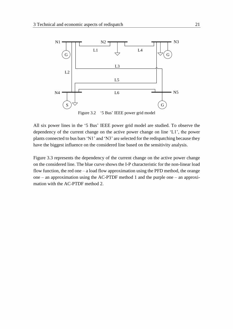
for the sensitivity analysis, includes [31] and is shown in Figure 3.2:
5 bus bars (‘N4’ is a slack node)
3 power plants
6 lines
3 loads
3 Technical and economic aspects of redispatch 21
N3
N5
G G
S G
N1 N2
N4
L1
L2
L3
L4
L5
L6
Figure 3.2 ‘5 Bus’ IEEE power grid model
All six power lines in the ‘5 Bus’ IEEE power grid model are studied. To observe the
dependency of the current change on the active power change on line ‘L1’, the power
plants connected to bus bars ‘N1’ and ‘N3’ are selected for the redispatching because they
have the biggest influence on the considered line based on the sensitivity analysis.
Figure 3.3 represents the dependency of the current change on the active power change
on the considered line. The blue curve shows the I-P characteristic for the non-linear load
flow function, the red one – a load flow approximation using the PFD method, the orange
one – an approximation using the AC-PTDF method 1 and the purple one – an approxi-
mation with the AC-PTDF method 2.

3 Technical and economic aspects of redispatch 22
Figure 3.3 I-P characteristics for the line ‘L1’ in the ‘5 Bus’ IEEE test network model
Based on the I-P characteristics for the line ‘L1’, all sensitivity analysis methods have
small deviations from the power flow function so that all curves are close to each other.
Therefore, their zoomed representation to show which method is more accurate is given
in Figure 3.4.
Figure 3.4 I-P characteristics for the line ‘L1’ in the ‘5 Bus’ IEEE test network model
(zoomed representation)
-2,74
-1,74
-0,74
0,26
1,26
2,26
-2000 -1500 -1000 -500 0 500 1000 1500 2000
Cu
rren
t d
evia
tio
n i
n k
A
Active power deviation in MW
load flow PFD AC-PTDFs_1 AC-PTDFs_2
2,56
2,6
2,64
2,68
2,72
1900 1920 1940 1960 1980 2000
Cu
rren
t dev
iati
on i
n k
A
Active power deviation in MW
load flow PFD AC-PTDFs_1 AC-PTDFs_2

3 Technical and economic aspects of redispatch 23
Obviously, the PFD approximates the non-linear load flow function most accurately in
this test case. However, the AC-PTDF methods 1 and 2 provide accurate results as well.
Furthermore, to observe the dependency of the current change on the active power change
on line ‘L3’, the power plants with the biggest influence on the considered line, which
are connected to bus bars ‘N1’ and ‘N5’, are selected for the redispatch realization. Figure
3.5 represents the dependency of the current change on the active power change on line
‘L3’.
Figure 3.5 I-P characteristics for the line ‘L3’ in the ‘5 Bus’ IEEE test network model
Here, the approaches provide small deviations as well as by the approximations in the
previous case. For this reason, a zoomed representation of the I-P characteristics for the
line ‘L3’ is given on Figure 3.6.
-4,46
-3,46
-2,46
-1,46
-0,46
0,54
1,54
2,54
3,54
-2000 -1500 -1000 -500 0 500 1000 1500 2000
Curr
ent
dev
iati
on i
n k
A
Active power deviation in MW
load flow PFD AC-PTDFs_1 AC-PTDFs_2

3 Technical and economic aspects of redispatch 24
Figure 3.6 I-P characteristics for the line ‘L3’ in the ‘5 Bus’ IEEE test network model
(zoomed representation)
In this case, the PFD method provides the most accurate results again. But the AC-PTDF
approaches have only small deviations too.
3.1.3.2 Simplified grid model of the ENTSO-E area
The simplified grid model of the ENTSO-E area, which is described in detail in chap-
ter 5.1.2 and shown in Figure 5.3, is also utilized to compare the introduced methods for
the sensitivity analysis.
To observe the dependency of the current change on the active power change on the dou-
ble power line between bus bars ‘1’ and ‘2’, the power plants with the biggest influence
on the considered line, which are connected to bus bars ‘1’ and ‘2’, are selected for the
redispatching. Figure 3.7 represents the dependency of the current change on the active
power change on this power line.
4,18
4,23
4,28
4,33
4,38
4,43
1900 1920 1940 1960 1980 2000
Cu
rren
t d
evia
tio
n i
n k
A
Active power deviation in MW
load flow PFD AC-PTDFs_1 AC-PTDFs_2

3 Technical and economic aspects of redispatch 25
Figure 3.7 I-P characteristics for the line power line between bus bars ‘1’ and ‘2’
Here, the PFD provides a very accurate approximation, while the AC-PTDF methods 1
and 2 approximate the non-linear load flow function with large deviations.
In addition, to observe the dependency of the current change on the active power change
on the double power line between bus bars ‘11’ and ‘19’, the power plants with the biggest
influence on the considered line, which are connected to bus bars ‘11’ and ‘19’, are se-
lected for the redispatch realization. Figure 3.8 represents the dependency of the current
change on the active power change on this power line.
-4,02
-3,02
-2,02
-1,02
-0,02
0,98
1,98
2,98
3,98
-2000 -1500 -1000 -500 0 500 1000 1500 2000
Curr
ent
dev
iati
on
in
kA
Active power deviation in MW
load flow PFD AC-PTDFs_1 AC-PTDFs_2

3 Technical and economic aspects of redispatch 26
Figure 3.8 I-P characteristics for the line power line between bus bars ‘11’ and ‘19’
Obviously, the sensitivity analysis methods provide similar results as well as in the pre-
vious case.
3.1.3.3 Conclusions
Based on the simulation results for the standard IEEE test power grid models and simpli-
fied ENTSO-E grid model, the PFD approach provides the most accurate approximations
of the non-linear load flow function in all test models. Its maximum deviation is around
9% in case of a high load in the simplified grid model of the ENTSO-E area. However,
the AC-PTDF methods 1 and 2 can have extremely large approximation deviations up to
100% and more in the utilized power grid models. Therefore, in this work, the calculation
of the network sensitivity analysis is done by the PFD method.
-4,55
-3,55
-2,55
-1,55
-0,55
0,45
1,45
2,45
3,45
4,45
-2000 -1500 -1000 -500 0 500 1000 1500 2000
Curr
ent
dev
iati
on
in
kA
Active power deviation in MW
load flow PFD AC-PTDFs_1 AC-PTDFs_2

3 Technical and economic aspects of redispatch 27
3.2 Economic aspects of redispatch
Since redispatching is a very often used remedial action by the TSOs and can cause enor-
mous costs, it should be realized cost-efficiently to avoid high expenses. In this respect,
some economic aspects, e.g. electricity generation costs, start-up and shut-down costs of
the power plants, which participate in the redispatch, should be considered. [4]
3.2.1 Levelized costs of electricity
For the redispatch realization it is important to consider the so-called levelized costs of
electricity (LCOE) cLCOE. These costs need to be spent on an energy conversion from any
form of energy to electricity [33]. They are usually given in euros per kWh and consist
of:
initial investment
costs of capital
operating cost
costs of fuel
maintenance cost
The total LCOE for different conventional power plant types are provided in Table
3.1 [34], [35].
Table 3.1 LCOE for different conventional power plant types [34]
Power plant LCOE in €/MWh
\Power plant types average min max
Lignite-fired power plants 63 46 80
Hard coal-fired power plants 81 63 99
Combined cycle gas turbine power plants 89 78 100
Gas turbine power plants 165 110 219
3.2.2 Power plant cycling costs
Furthermore, the power plant cycling costs (PPCC) can be also taken into account by the
redispatch realization. Cycling of a power plant is its operation depending on different

3 Technical and economic aspects of redispatch 28
load levels. Here, the power plants are permanently switched on and off, which can cause
an equipment damage because of large pressure and thermal stresses during these pro-
cesses. The PPCC can be classified in general in five groups [36], [37]:
fuel, auxiliary services and CO2 emission costs related to the start-up, also called
direct start-up costs
equipment replacement and maintenance costs related to the start-up, also called
indirect start-up costs
equipment replacement and maintenance costs related to the load following, also
called ramping costs
forced outage costs related to the start-up i.e. opportunity costs for the power gen-
eration during a power plant outage
heat rate effects related to the power plant cycling
Therefore, the total PPCC csu,i can be calculated as shown below:
su, su_dir, su_indir, ramp, fo, hr_incr,i i i i i ic c c c c c (3.18)
where csu_dir,i is the direct start-up costs, csu_indir,i is the indirect start-up costs, cramp,i is the
ramping costs, cfo,i is the forced outage costs, chr_incr,i is the costs due to the heat rate
increase.
Furthermore, the indirect start-up costs are depending on the time, during which the power
plant was offline: the longer it was offline, the higher the indirect start-up costs. There
are three types of the power plant start-up regarding the offline time [38]:
hot start if the power plant was offline less than 24 hours before the start-up process
warm start if the power plant was offline between 25-119 hours before the start-up
process
cold start if the power plant was offline for 120 hours or more before the start-up
process
The indirect start-up costs are an exponential function based on the start-up loss depend-
ency from the offline time t of the power plant time [39], [40] and can be determined as
follows [41], [42]:
su_indir, su_indir,max, (1 e )i t
i ic c
(3.19)

3 Technical and economic aspects of redispatch 29
where csu_indir,max,i is the maximum of the indirect start-up costs for the power plant i and
λi is the heat-loss coefficient which is defined between 0 and 1.
Figure 3.9 shows the dependency of the indirect start-up costs from the time during which
the power plant was offline (the green curve). The orange lines are average values of the
indirect start-up costs for three types of the power plant start-up.
Figure 3.9 Indirect start-up cost function [41]
The total PPCC for different conventional power plant types are provided in Table 3.2.
These costs were originally calculated in US dollars for the United States in 2011 [36].
However, for this work, they are converted into euros regarding the average dollar ex-
change rate in 2011.
Table 3.2 Cycling costs for different conventional power plant types [36]
Power plant cycling cost types Direct Indirect Ramping
Costs in €/MW
\Power plant types
hot
start
warm
start
cold
start
ave-
rage min max
ave-
rage min max
Coal-fired power plant (small
subcritical)
7 9 12 96 67 143 10 7 11
Coal-fired power plant (large
subcritical)
9 13 17 55 38 65 11 6 13
Coal-fired power plant (super
critical)
11 19 23 53 40 65 8 5 10
Time hot warm cold
Cost
cstart-up_indir,max
average indirect start-up costs for warm start

3 Technical and economic aspects of redispatch 30
Power plant cycling cost types Direct Indirect Ramping
Gas-based combined cycle
power plant
- - - 41 25 60 1.5 0.7 1.6
Gas-fired power plant 1 1 1 63 19 74 3.5 2 6
Power plant with aero-deriva-
tive gas turbine
3 3 3 18 9 44 0.5 0.4 1.2
Gas-fired steam power plant 6 10 15 41 28 52 6 3.4 7
Power plant cycling cost types Forced outage
Costs in €/MW
\Power plant types
hot
start
warm
start
cold
start
Coal-fired power plant (small
subcritical)
1 2 3.4
Coal-fired power plant (large
subcritical)
0.4 0.5 1.4
Coal-fired power plant (super
critical)
0.3 0.6 0.9
Gas-based combined cycle
power plant
0.3 0.6 0.6
Gas-fired power plant 0.5 1.7 1
Power plant with aero-deriva-
tive gas turbine
0.8 0.8 0.9
Gas-fired steam power plant 0.2 0.5 0.8
Due to the heat rate increase, the costs can be are neglected because they are very small
compared to other cost types [36].
The indirect PPCC for different conventional power plant types are provided in detail in
Table 3.3. These costs are converted into euros as well.
Table 3.3 Indirect cycling costs for different conventional power plant types [36]
Power plant start-up types Hot start Warm start Cold start
Indirect cycling costs in €/MW
\Power plant types
ave-
rage min max
ave-
rage min max
ave-
rage min max
Coal-fired power plant (small
subcritical)
68 57 94 113 80 130 106 63 205
Coal-fired power plant (large
subcritical)
42 28 49 47 40 56 75 45 89
Coal-fired power plant (super
critical)
39 28 45 46 39 64 75 52 86
Gas-based combined cycle
power plant
25 20 40 40 23 67 57 33 73
Gas-fired power plant 23 16 34 91 19 104 74 22 85

3 Technical and economic aspects of redispatch 31
Power plant start-up types Hot start Warm start Cold start
Power plant with aero-deriva-
tive gas turbine
14 9 44 17 9 44 23 9 44
Gas-fired steam power plant 26 18 30 42 26 63 54 39 64
Due to difficulty of the PPCC calculation, the total PPCC are rarely involved in making
decisions of the unit commitment by the system operators. Therefore, only the direct start-
up costs are usually considered even though they can be a small part of the total
PPCC. [37]
3.2.3 Shut-down costs
In addition, the power plant shut-down costs (PPSDC) csd for different conventional
power plant types can be considered by the redispatch realization as well. However, in
contrast to the power plant cycling costs, they are considerably lower. [43], [44], [45]
The total PPSDC for different power plant types are provided in Table 3.4 [45].
Table 3.4 PPSDC for different conventional power plant types [45]
Power plant shut-down costs in €/MW
\Power plant types average
Coal-fired steam power plants 1.6
Combined-cycle gas turbines 2.2

32
4 Optimization methods
First of all, to solve an optimization problem, a suitable optimization method must be
chosen. The selected technique should provide sufficiently accurate solutions in a short
time. The choice of the optimization algorithm strongly depends on the formulation of
the optimization problem, resp. of its objective function and constraints.
There is a wide range of optimization methods for solving different optimization prob-
lems. Therefore, the big challenge in this field is to extract a suitable optimization tech-
nique from the many existing methods. Furthermore, some optimization algorithms are
specifically developed for a certain kind of optimization task, e.g. the linear program-
ming for problems with a linear criteria and linear constraints. In addition, various opti-
mization methods can usually be used to solve one specific problem.
The optimization techniques, which are suitable for the redispatch optimization, are in-
troduced in this chapter.
4.1 Linear programming
The Linear Programming (LP) is a very common optimization technique to solve opti-
mization problems, which include only a linear objective function (4.1) and linear con-
straints (4.2). It is used in different areas, e.g. industry, medicine, economy, engineering,
computer science etc. The main objective of the LP is to maximize or minimize the linear
function over a polyhedron. [46], [47], [48], [49], [50]
1 2 1 1 2 2
1
, ..., ...
or
, ( 1,2..., )
n n n
n
j j j
j
f x x x c x c x c x
f x c x j n
(4.1)
subject to:

4 Optimization methods 33
11 1 12 2 1 1
21 1 22 2 2 2
1 1 2 2
1
...
...
...
...
or
, ( 1,2..., )
n n
n n
m m mn n m
n
ij i i
j
a x a x a x b
a x a x a x b
a x a x a x b
a x b i m
(4.2)
where f(xj) is the linear function, xj – the searched variables, aij, bi, cj – the real numbers,
n – the number of function variables, m – the number of constraints.
Based on equations (4.1) and (4.2), the LP problem with the objective function c can be
formulated in the following standard matrix form [46], [47], [48], [49], [50]:
Tminx
c x (4.3)
subject to:
Aх b (4.4)
where the linear constraints are expressed by the vector of the searched variables x, matrix
of the constraint system A and vector of the constraint restrictions b.
4.1.1 Simplex algorithm
The simplex method or simplex algorithm is a frequently used algorithm for solving opti-
mization problems of the LP developed by George Danzig in 1947 [46], [47]. This method
finds an exact solution of an optimization problem after a finite number of iteration steps
or determines its infeasibility.

4 Optimization methods 34
4.1.1.1 General approach
The simplex algorithm solves optimization problems with the objective function c and
constraints in the form described by equations (4.3) and (4.4). It consists of two main
steps. [46], [47]:
1. determination of a starting solution, which must fulfil the constraints (usually not
the optimal solution) or infeasibility of the optimization problem.
2. iterative improvement of the current solution of the optimization problem until an
optimal solution is found, i.e. an improvement of the objective function is not
possible anymore.
At each iteration step the so-called simplex tableau T is calculated anew to find the most
suitable edge of the polyhedron, resp. the optimal solution [4], [15]:
T 0 f
A I bT
c (4.5)
with the identity matrix I and value of the cost function f, which is determined as shown
in equation (4.3).
For every iteration the pivot element in the simplex tableau must be found. Here, the pivot
column is the column with the smallest negative coefficient of cT and the pivot row is the
row with the smallest nonnegative quotient of b and the pivot column of A. Then the pivot
column is transformed to a unit vector regarding the pivot element. These calculation
steps are equivalent to the Gaussian elimination, resp. to the steps by solving a linear
system of equations. They lead to a new optimization problem solution, resp. to a new
edge of the polyhedron with more optimal objective function value.
4.1.1.2 Performance
Nowadays, the simplex algorithm is widely and constantly utilized in various fields
around the world to solve linear programming problems. This is the greatest proof of its
high performance. There are several main advantages, which make the simplex extremely
popular [46], [47]:

4 Optimization methods 35
It is based on a simple calculation method and is easily understandable.
It is easy to implement.
It has a low computation time, especially by small linear programming problems.
It considers different factors and restrictions of the optimization problem by every
iteration step instead of guessing the optimal solution.
Nevertheless, there are some disadvantages of the simplex algorithm, which should be
considered by choosing an optimization method:
It can only be utilized for certain linear programming tasks, which requires an ad-
aptation of the optimization problem.
It is not the fastest analytical optimization method.
During solving the optimization problem an infinite loop can occur by a careless
choice of the pivot elements.
4.1.2 Linear redispatch optimization
4.1.2.1 Objective function of the redispatch optimization problem
Here, the costs c for the realization of the redispatch, which should be minimized as
shown in equation (4.3), is used as the objective function for the considered optimization
problem and is formulated as follows [4], [15], [17], [46], [47]:
1 1
ij ij
G G
i j
c P c
(4.6)
with
incr, red,ij i jP P P (4.7)
incr, red,ii jjc c c (4.8)

4 Optimization methods 36
where ΔPij is the amount of the power generation change for every possible power plant
pair during the redispatching, Pincr,i, Pred,j are the amount of the power generation in-
crease/reduction for each power plant, Δcij is the costs in €/MWh, which must be spent
for the power generation change by every possible power plant pair, cincr,i, credj are the
cost, which must be spent/saved for the increasing/reducing of the power generation for
each power plant and G is the number of the power plants in the power grid.
4.1.2.2 Constraints of the redispatch optimization problem
The main constraint for the introduced redispatch optimization problem is considering
the electric network state, i.e. power flow, and node impact on the congested line. The
easiest and most efficient way to formulate this constraint is a linearization of the non-
linear power flow equations using the network sensitivity analysis:
1
cong
1
G G
j
ij ij
i
P P
(4.9)
with
incr, red,ii jj (4.10)
where Δσij is the difference between the sensitivity coefficients for every possible power
plant pair during the redispatching, Δσincr,i, Δσred,j are the sensitivity coefficients for each
power plant.
In this work, the PFD, which is introduced in chapter 3.1.2, is used to calculate the net-
work sensitivities, resp. to formulate the first constraint in equation (4.9) of the considered
redispatch optimization problem.
The further important constraints for the optimization problem are the consideration of
the power plant redispatch potentials, which can be utilized during the redispatch realiza-
tion. These constraints consider the maximum and minimum active powers, which can be
generated by the power plants.

4 Optimization methods 37
RP+,
1 1
G G
ij ji i
j j
P P P
(4.11)
RP-,
1 1
G G
ji ij i
j j
P P P
(4.12)
where PRP+,i and PRP-,i are the positive and negative redispatch potentials of the power
plant i.
4.1.3 Sequential simplex
4.1.3.1 General approach
The sequential simplex (SS) is an extension of the standard simplex algorithm and was
proposed by W. Spendley, G.R. Hext and F.R. Himsworth in 1962. This technique utilizes
the simplex sequentially, i.e. each subsequent simplex run starts with the last working
point of the previous run, resp. they both always have one common edge. Therefore, cal-
culation errors can be completely remedied in this way. [51], [52]
The SS was further developed by J. A. Nelder and R. Meadf in 1965. In this approach,
the objective function with n variables is minimized compressing the function values at
n+1 vertices, resp. positions p of the standard simplex. Thereby, the highest vertex ph with
the maximum value must be replaced by another working point. Therefore, the SS adjusts
itself to the local minimum to finally find the global minimum.
Firstly, the initial vertex p1 is randomly chosen. Then the remaining vertices pi need to be
scaled by [52] [53]:
( 1)
1 u i
i ip p (4.13)
where i=2,…,n+1, λ i – the positive constants and u – the unit vector.
Furthermore, the so-called centroid of the simplex pc should be calculated without con-
sideration of the highest vertex as follows [52]:

4 Optimization methods 38
1
c
2
n
i
i
p p (4.14)
The reflection pr, which is the main operation of the SS, is determined by:
r c 1 c h( ) p p p p (4.15)
where α1 is the reflection coefficient, which is greater than 0 and is calculated as follow-
ing [52]:
r c1
h c
p p
p p (4.16)
If the function value fr of the reflection pr is smaller than the function value fl of the lowest
vertex pl, the so-called expansion must be done:
e c 2 r c( ) p p p p (4.17)
with
e c2
r c
p p
p p (4.18)
If the function value fe of the expansion pe is smaller than the function value fl of the
lowest vertex pl, the highest vertex ph is replaced by the expansion. Here, the reflection
pr must be recalculated taking into account the new expansion value.
If the function value fe is greater than the function value fl, the highest vertex ph is replaced
by the reflection. Then the reflection pr must be recalculated as well.
However, if the function value fr of the reflection pr is greater than the function value fl of
the lowest vertex pl, the highest vertex ph is immediately replaced by the reflection pr.
After that the so-called contraction pcontr is calculated as follows:
c 3 h c( ) contrp p p p (4.19)

4 Optimization methods 39
where α3 is the contraction coefficient, which is determined by:
contr c3
h c
p p
p p (4.20)
with
30 1 (4.21)
If the function value fcontr of the contraction is smaller than the minimum value of the
function values fh and fr, the highest vertex ph is replaced by the contraction pcontr. Here,
the reflection pr must be recalculated again.
Finally, if the fcontr is greater than the minimum value of the fh and fr, all positions pi should
be replaced using:
l
2
i
i
p pp (4.22)
Then the reflection must be recalculated.
If the global minimum is reached, the iterative process is stopped.
4.1.3.2 Algorithm adaptation for the non-linear redispatch optimization problem
To avoid deviations in the congestion power calculation, which are caused by the utiliza-
tion of the sensitivity analysis, the SS is used in this work as well.
The optimization begins from a run of the standard simplex taking into account the linear
redispatch optimization, which is described in detail in chapter 4.1.2. Here, the found
power changes of power plants for the redispatch realization are used to create a new
working point of the power grid. Then the power flow of this new working point is deter-
mined using the non-linear load flow equations.

4 Optimization methods 40
If there is deviation in the congestion power calculation, this deviation is utilized as the
congestion power on the congested line in equation (4.9) for the next run of the simplex.
Furthermore, before the next run, the network sensitivity analysis for the new working
point are calculated again. Therefore, the new sensitivity coefficients are taken for the
redispatch optimization using equation (4.9). In addition, the power plant redispatch po-
tentials are recalculated as well. This procedure repeats until the network congestion is
completely remedied.
4.2 Genetic algorithm
The genetic algorithm (GA) is a stochastic evolutionary optimization method, which is
based on principles of Darwin's theory of biological evolution such as genetic inheritance
and natural selection. It was developed by Prof. John Holland and his students at the Uni-
versity of Michigan in the early 1970s. The GA is very well suited for solving highly
nonlinear optimization problems and is able to find the global optimal solution in a com-
plex search space. It is utilized in a variety of areas, e.g. engineering, robot technology,
bioinformatics, computer science, economy, chemistry, transport etc. [54], [55], [56],
[57], [58], [59], [60], [61]
4.2.1 Evolutionary optimization algorithms
The Evolutionary algorithms (EA) are a subset of stochastic optimization methods, which
are based on evolutionary mechanisms such as a selection, mutation, recombination and
reproduction. The EAs cannot usually find the best solution but a well approximating one
for every optimization problem type. Furthermore, they are easily implementable. This
all makes them applicable in a broad range of fields. [55], [56]
The recombination and mutation operators of the EAs can extend the search space. But it
does not provide any guarantee that the current problem solution will be improved. How-
ever, the search procedure always moves to a global optimum by means of the selec-
tion. [57]

4 Optimization methods 41
There are plenty of evolutionary algorithm types and variations. The evolutionary algo-
rithms differ mainly in the genetic representation, genetic operators and objective func-
tion of the optimization problem.
In this work, the genetic algorithm and its variation are introduced and evaluated. The
basic principles of these optimization methods are described in this chapter
4.2.2 General approach
In contrast to the simplex algorithm, the GA can solve optimization problems with the
fitness function c and constraints which can be formulated by linear, non-linear, discrete
or discontinues equations [4], [15], [54], [57]:
maxx
f x (4.23)
Assumed:
A х b (4.24)
As well as all evolutionary algorithms, the GA is an iterative process, which begins with
the generation of an initial population. This start population consists of chromosomes
which are randomly created. Furthermore, before the population initialization, the objec-
tive function, constraints of the optimization problem and GA parameters must be de-
fined. Then the recombination of the best chromosomes is realized, resp. the strongest
individuals produce an offspring. In the next step, a new generation is created based on
the best individuals and their offspring. After that the new generation mutates and the
strongest individuals of this generation are chosen for the next iteration step. The above
process repeats until break conditions, e.g. finding an acceptable solution or exhaustion
of the iteration steps, are fulfilled. A flowchart of the described iterative process is given
in Figure 4.1 [4], [54], [55], [59]

4 Optimization methods 42
Initial population
generation
Objective function,
constraints and GA
parameters
Mutation
Selection
Break
conditions
Recombination
Best solution
Figure 4.1 Flowchart of the genetic algorithm
4.2.2.1 Recombination
There are various methods for mating the best individuals/chromosomes in the GAs. But
the simplest and in many cases well working mating approach is choosing one crossover
point in the two parent chromosomes cm and cf [54].

4 Optimization methods 43
m m1 m2 m m
f f1 f2 f f
[ , ,..., ,..., ]
[ , ,..., ,..., ]
crp n
crp n
c c c c
c c c c
c
c (4.25)
where cm1, cm2,…cmn are the variables of the ‘mother’ chromosome, cf1, cf2,…cfn – the
variables of the ‘father’ chromosome, n – the number of the chromosome variables and
cmcrp, cfcrp – the crossover point, i.e. the chromosome variables are randomly exchanged
in the crossover point. Therefore, two new offspring chromosomes coffspr1 and cfoffspr2 are
produced:
offspr1 m1 m2 f f
offspr2 f1 f2 m m
[ , ,..., ,..., ]
[ , ,..., ,..., ]
crp n
crp n
c c c c
c c c c
c
c (4.26)
However, the big disadvantage of this approach that there is no new genetic material in
the offspring at all: the offspring is only a new combination of the parents. Consequently,
a new genetic material can only appear by a mutation.
To solve this problem an extrapolation can be used in the introduced crossover method,
i.e. new variable values cnew1 and cnew2, which are based on different combinations of the
parent variable values, are integrated in the offspring [54].
new1 m m f
new2 f m f
crp crp crp
crp crp crp
c c c c
c c c c
(4.27)
where β is the random number between 0 and 1.
Then these calculated values are integrated into equation (4.25) instead of the crossover
point as given by
offspr1 m1 m2 new1 f
offspr2 f1 f2 new2 m
[ , ,..., ,..., ]
[ , ,..., ,..., ]
n
n
c c c c
c c c c
c
c (4.28)
If the crossover point is the first chromosome variables, the remaining variables of the
parent chromosomes to the right are exchanged. If the crossover point is the last chromo-
some variables, the remaining variables of the parent chromosomes to the left are ex-
changed. [54]

4 Optimization methods 44
After the recombination a new generation, which can consist of the parent and offspring
chromosomes are created.
4.2.2.2 Mutation
With the help of the recombination the GA can find a global minimum very fast. How-
ever, such approximate solutions are not enough to fulfill the task in many cases: a local
minimum must be found as well. For this reason, a mutation operator is utilized in the
GAs. It introduces a new genetic material in a new generation to expand the search
area. [54], [55], [57]
In the first place, a mutation rate must be chosen. In general, the mutation is a quite rare
phenomenon in the biology. Consequently, the mutation rate should be a small value.
However, it is not possible to find one optimal value of the mutation rate for all optimi-
zation problems. Therefore, the set value should be often adapted to the considered task.
The most utilized approach to find the new mutated chromosome variable cmut uses a
normal/Gaussian distribution function and is given by [54]:
mut old 0,1c c N (4.29)
where cold is the selected chromosome variable for the mutation, σ – the standard deviation
of the Gaussian distribution function, N(0,1) – the standard Gaussian distribution with the
mean 0 and variance 1.
4.2.2.3 Selection
At the end of each iteration, after the mutation, the strongest individuals of the population
are chosen, resp. a new generation is created again. This generation is used for the recom-
bination during the next iteration. The iterative process repeats until the break conditions
are fulfilled.

4 Optimization methods 45
4.2.3 Constraint handling
The bulk of optimization problems not only consist of the objective function, but also of
many different linear, non-linear etc. constraints. Therefore, constraint handling, i.e. han-
dling of constraint equations in the optimization method, should be integrated in the GAs.
However, there is no universal constraint handling approach, which could be used in
every optimization technique. The constraint handling method should be chosen based
on the optimization method type and considered optimization prob-
lem. [62], [63], [64], [65]
There are various constraint handling , which can be used for the GAs. They can be clas-
sified in the following groups [62], [65]:
utilization of penalty functions
search of feasible solutions
distinction between feasible and infeasible solutions
hybrid methods
The constraint handling methods, which are based on the penalty functions, are mostly
used in the GAs because they are quite simple, easily implementable and well-working
for many optimization problems. They convert a constrained optimization problem to an
unconstrained problem by penalizing unfeasible solutions [62], [63], [64], [65].
if
, other i e(
s)
w
f Ff
f penalty
x xx
x x (4.30)
where penalty(x) is the penalty parameters and F – the feasible area. If the considered
optimization problem is a minimization problem and there is no violation of the con-
straints, penalty(x) is 0. Otherwise, it is a positive value.
In this chapter, the most common constraint handling approaches are introduced.

4 Optimization methods 46
4.2.3.1 Death penalty
The death penalty method is the simplest and mostly used approach for handling con-
straint optimization problems. It sorts out every unfeasible solution from the generation
by penalizing the unfeasible solutions in such a way, that this generation can only consist
of the feasible solutions. This method works especially well if the feasible area belongs
to the sensible search space. However, if the optimization problem is highly constrained,
the death penalty approach has a high computation time and the proposed best solution
might not be accurate enough. [62]
4.2.3.2 Static penalty
The static penalty method is also a quite simple approach for handling the constraint op-
timization problem. It penalizes the unfeasible solutions as well as the death penalty
method. However, in this approach some levels of the constraint violation with own pen-
alty coefficient must be chosen. The more constraints are violated by the unfeasible solu-
tion, the higher the penalty value for this solution. [62], [65]
1 1
1 if constraint is violatedwith
0 if constraint is fulfilled
l m
ij j
i j
j
j
f f C d
d j
d j
x x
(4.31)
where Cij is the penalty coefficient, i – the current violation level, j – the current con-
straint, l – the level number and m – the constraint number.
However, in this approach a high number of parameters, resp. m(2l+1) parameters, must
be selected and applied. This makes the utilization of the static penalty method quite dif-
ficult. Furthermore, the accuracy of the solutions strongly depends on the chosen values
of these parameters. [65]

4 Optimization methods 47
4.2.3.3 Dynamic Penalty
As opposed to the previous approach, in the dynamic penalty method the penalties change
over the time, resp. in every iteration step i. The penalizing of the unfeasible solutions is
given by:
1
1 if constraint is violatedwith
0 if constraint is fulfilled
m
j
j
j
j
f f Ci d
d j
d j
x x
(4.32)
where C and α are the user-defined constants with the recommended values: C = 0.5 and
α = 1 or 2. [62], [65]
The accuracy of the solutions strongly depends on the chosen values of the parameters α
and β. Furthermore, this approach quite often cannot find any feasible solution or finds a
solution, which is not accurate enough. [62], [65]
There are many other methods for the constraint handling. But they are not described in
this chapter because they are not considered in this work.
4.2.4 Performance
The genetic algorithm is widely used for solving different optimization problems in var-
ious fields, e.g. engineering, robotics, databases, neural networks, chemistry, bioinfor-
matics, transport, investment and game strategies etc., because it has the following ad-
vantages [54]- [58]
It is easily implementable.
It can be easily adapted for the considered optimization problem.
It can work with a large number of variables.
It works with continuous and discrete variables.
It is very stable.

4 Optimization methods 48
Nevertheless, it has some disadvantages, which should be considered by choosing the
optimization method:
It is computational intense.
It can find an optimal solution, which is not accurate enough.
It has many parameters, which must be selected by the user.
4.2.5 Non-linear redispatch optimization problem for the GA
Firstly, the linear fitness function c of the redispatch optimization problem for the GA
should be minimized by the utilization of equation (4.6) as well as for the simplex algo-
rithm.
The main constraint is taking into account the electric network state and node impact on
the congested line. However, the electric network state can be described by the non-linear
power flow equations, which are not linearized in comparison to the formulation of the
redispatch optimization problem for the simplex algorithm.
The power plant potentials, which can be used for the redispatch realization, are consid-
ered with the help of equations (4.11) and (4.12) as well.
Furthermore, in the first place, the lowest-cost power plants are used in an ascending
order of their total costs to cover the load consumption. This process is called a merit
order. However, the merit order data can sometimes include errors, in which the more
expensive power plants are used instead of cheaper one. In this case, a profit could be
theoretically made by the utilization of the redispatch, which is not possible in the prac-
tice. Hence, based on equation (4.8), the redispatch total costs for each power plant pair
must be positive:
incr, red, 0i jc c (4.33)
Moreover, the cost objective function c must be equal or greater to 0:
0c (4.34)

4 Optimization methods 49
In addition, the start-up and shut-down of power plants can be taken into account by an
implementation of the so-called integer variables into the redispatch optimization prob-
lem. Here, the integer variables can take only binary values 0 or 1.
In this case, the costs c for the realization of redispatch considering the PPCC and PPSDC,
which might be minimized, is utilized as the non- linear fitness function for the considered
optimization problem and is formulated as follows [4], [15], [17], [40]-[42], [44], [66],
[67], [68]:
su sd
su, sd,
1 1 1 1
G GG G
ii i i i
i j
j ij
i i
P cc c su c sd
(4.35)
where Gsu, Gsd are the number of the power plants, which need to be started-up and shut
down, sui and sdi are the binary variables, which are 1 if the power plants are started-up
and shut down, otherwise they are equal to 0.
If the power plant, which participates in the redispatch, should be started-up, its total
generated active power Pi must be equal or less to its maximum active power Pmax,i and,
at the same time, equal or greater to its minimum active power Pmin,i, which are multiplied
with the binary status variable su. [66]
max, ii iP P su (4.36)
min, ii iP P su (4.37)
Finally, the PPSDC are neglected in this work because they are very small compared to
other cost types (see Table 3.4).
4.2.6 Algorithm adaptation for the non-linear redispatch optimization
problem
First of all, the GA is developed and adapted for the described redispatch optimization
problem to compare its results with results of the remaining optimization techniques,
which are utilized in this work. Furthermore, the GA is tested in a small network model

4 Optimization methods 50
and simplified network model of the ENTSO-e power grid, which are described in detail
in chapter 5.1.
There are various ways to implement the GA However, the choice of the genetic algo-
rithm type primarily depends on the formulation of the considered optimization problem.
The previously introduced non-linear optimization problem for the redispatch realization
consists of continuous variables. Therefore, in this work, the so-called continuous genetic
algorithm, which is described in detail in chapter 4.2.2 and shown by the flowchart in
Figure 4.1, is implemented to solve this task.
In the developed GA, a randomly created initial population consists of the chromosomes,
which include the possible power generation changes for all power plant combinations of
the considered network models. Here, the positive and negative redispatch potentials of
each power plant pair must be taken into account. Furthermore, the population individuals
include binary values for the start-up and shut-down status of the power plants. Hovewer,
these binary combinations are not random values. They are generated according to the
chosen power plant pairs.
To produce new offspring chromosomes, the approach of the one crossover point of two
parent chromosomes is used based on equations (4.25) and (4.26). Furthermore, to include
a new genetic material in the offspring, new values, which are based on different combi-
nations of the parent variable values, are integrated in the offspring by equation (4.27).
Therefore, these new values replace the crossover point as shown in equation (4.28). In
every iteration step a new generation is built based on the parent and offspring chromo-
somes.
The mutation is implemented in the GA to find a local minimum in the search space using
equation (4.29). Here, the mutation rate is adaptive and depends on the optimization prob-
lem, i.e. on the power plant number and population size.
After the mutation, the strongest population individuals are chosen to create a new gen-
eration for the next iteration step. This iterative process repeats until the break conditions
are fulfilled.
As already mentioned, the parameters of the evolutionary algorithms usually need to be
adopted for the considered optimization problem. The developed GA for the introduced
non-linear redispatch optimization problem with the consideration of the power flow
equations and PPCC is parameterized as follows:

4 Optimization methods 51
The population consists of 200 individuals: 100 strongest parent chromosomes and
their 100 offspring.
The mutation rate is 0.4 by reference to the power plant pair number 64 and popu-
lation size 200.
The standard deviation of the Gaussian distribution function σ is 0.05.
The iteration number is 10000. However, if the best solution cannot be improved
during many iterations, the iterative process is stopped.
The static penalty for the constraint handling is 1000000.
4.3 Mean Variance Mapping Optimization
The Mean Variance Mapping Optimization (MVMO) is a new stochastic optimization
method which is based on the GA. But a novelty in this optimization technique is the
utilization of the so-called mapping function (MF) for the mutation process. The MF is
based on mean and variance of some best solutions, which are saved in a continually
updated archive. The MVMO was developed by István Erlich in 2010 motivated by the
continually increasing complexity of the power system. Nevertheless, the MVMO has a
big potential to be used for solving optimization problems in different ar-
eas. [4], [69], [70], [71], [72], [73], [74], [75], [76]
4.3.1 General approach
The MVMO solves optimization problems with the same objective function and con-
straints as well as the GA, which are already described in equations (4.13) and (4.14).
However, as opposed to the GA, in the MVMO the offspring mutation is based on the
MP, resp. on the mean and variance of the best individuals of the population, which are
stored in an archive. The MF is usually defined in a range between 0 and 1. Hence, the
optimization variables must be scaled correspondingly to this range. In addition, during
the iteration process the shape of the MF is constantly modified according to the progress
of the best solution search. [4], [69]-[76]

4 Optimization methods 52
Therefore, the initial individuals xi are transformed into the new mutated generation xnew,i
using the MF. This transformation, resp. generation mutation, takes place according to
the following equation (4.38) and is shown in Figure 4.2 [4], [69]:
new, 1 0 01i x ix h h h x h (4.38)
xnew,i
xi = rand 10
1
Figure 4.2 Mapping function example [69]
Where the h-function hx is determined by:
21 11 e 1 e i ii i x sx s
x i ih x x
(4.39)
The parameters h1 and h0 are calculated by xi=1 and xi=0 using equation (4.39).
The mean of the variables �̅�𝑖 is established based on the archive with the n best solutions
as shown below:
1
1 n
i i
j
x x jn
(4.40)

4 Optimization methods 53
where xi is the best solution, which are stored in the archive.
The shape variables si are determined using the variance of the variables 𝑣𝑖:
lni i ss v f (4.41)
where fs is the factor for changing the shape of the MF and calculated by:
* 1s sf f rand (4.42)
with the smallest value fs* of the shape factor fs and the random value rand which is
between 0 and 1.
The variance of the variables 𝑣𝑖 is determined based on the archive with the n best solu-
tions xi as well the mean of the variables:
2
1
1 n
i i i ij
v x j xn
(4.43)
The shape factor fs is greater than 1 if the calculation accuracy must be increased and it is
less than 1 if the search of the solution shall be more global.
If the accurancy of the MVMO should be increased, the factor fs* can be calculated as
follows:
2
* * * *
start max start
max
s
if f f f
i
(4.44)
where fstart* is the smallest value of the factor fs
* and can be chosen between 0.9 and 1,
fmax* is its largest value and can be defined between 1 and 3, i is the current iteration and
imax is the maximum number of the iterations.
The shape variables si1 and si2 can be found using the algorithm, which is shown in Figure
4.3.

4 Optimization methods 54
si1 =si2=si
si > 0
si > di
di=di·Δd
yes
yes
di=di/Δd
no
rand ≥ 0,5
si1=si
si2=si
yes
si1=di
si2=si
no
end
no
Δd=(1+Δd0)+2·Δd0·(rand-0,5)
Figure 4.3 Algorithm for the determination of the shape variables
The start value of the variables di must be set before the iterative process starts and should
be defined between 1 and 1.5 based on the simulation experience [69]. The parameter di
is used instead of si1 to smooth the h-function.
Basically, if si is greater than 0, di is continually scaled with the factor Δd. If si is greater
than di, the factor di is scaled up with Δd, i.e. di becomes larger than at the beginning.
Here, the factor di remains close to the value of si. Otherwise, the factor di is scaled down
with Δd, i.e. di becomes smaller because Δd is always greater than 1.
In addition, the factor Δd oscillates around the value (1+Δd0) with decreasing amplitude
Δd0 as shown below:
4 Optimization methods 55
2
0 0,start 0,max 0,start
max
Δ Δ Δ Δi
d d d di
(4.45)
where Δd0,start is the smallest value of the factor Δd0 and Δd0,max is its largest value.
The factor Δd0 should be defined between 0.01 and 0.4 based on the simulation
experience [69].
The size of the archive for the MVMO should be small and usually varies between 2 and
5 of the currently best individuals. The utilization of a larger archive can lead to a too
strong influence of the best solutions on the orientation of the search.
4.3.2 Performance
The MVMO is a quite new optimization method, which is not yet widely used. In the
main, it is successfully utilized for different optimization problems in the power systems.
Basically, it has the same advantages and disadvantages as the GA because the MVMO
is based on the GA. The only difference is that the MVMO uses the MP for the mutation
process. Its most important advantage is the searching for a global solution with the con-
sideration of the best individuals, which makes this optimization method more efficient.
Nevertheless, a complicate mathematical description of the mutation process leads to a
longer computation time, resp. use of more computer resources. [69]
4.3.3 Non-linear redispatch optimization problem for the MVMO
In this work, the fitness function c of the redispatch optimization problem for the MVMO
should be minimized by the utilization of linear and non-linear equations (4.6) and (4.35)
in the same way as for the GA.
The main constraint of the redispatch optimization problem is taking into account the
electric network state and node impact on the congested line using the network sensitivity
analysis by equation (4.9) or the non-linear power flow equations as well as by the GA.

4 Optimization methods 56
The remaining constraints for the developed MVMO are already formulated by equa-
tions (4.11), (4.12), (4.33)-(4.37).
4.3.4 Algorithm adaptation for the non-linear redispatch optimization
problem
The MVMO algorithm is developed and adapted for the described redispatch optimiza-
tion problem to compare its results with the results of the remaining optimization tech-
niques, which are utilized in this work as well as the GA. Furthermore, it is also tested in
the already mentioned small network model and simplified network model of the EN-
TSO-e power grid (see chapter 5.1).
Due to the MVMO is a variation of the GA, producing the chromosomes and their
offspring is made in the same way as in the GA (see chapter 4.2.2). The so-called mapping
function , which is described in detail in chapter 4.3.1, is used during the mutation. There-
fore, the population individuals are transformed into a new mutated generation utilising
the MF in equation (4.38). To calculate the MF, the h-function, which is based on the
mean and variance of in the archive stored best solutions, must be dermenated using equa-
tions (4.39)-(4.45).
After the mutation the strongest population individuals are chosen to create a new gener-
ation for the next iteration step. This iterative process repeats until the break conditions
are fulfilled.
The developed MVMO for the introduced non-linear redispatch optimization problem is
parameterized as follows:
The population consists of 200 individuals: 100 strongest parent chromosomes and
their 100 offspring.
The mutation rate is 0.4 by reference to the power plant pair number 64 and popu-
lation size 200.
The archive size is 4.
The smallest value of the factor fs* is 0.9 and its greatest value is 1.5.
The smallest value of the factor Δd0 is 0.01 and its greatest value is 0.4.
The iteration number is 10000. However, if the best solution cannot be improved
during many iterations, the iterative process is stopped

4 Optimization methods 57
The static penalty for the constraint handling is 1000000.
4.4 Particle Swarm Optimization
The Particle Swarm Optimization (PSO) is a heuristic global optimization technique and
belongs to the family of the metaheuristic algorithms as well as the GA. This method is
based on population principles, resp. on the behavior of swarm individuals, which are
moving in the search-space according to a mathematical description of their position and
velocity. It was developed by J. Kennedy and R. Eberhart in 1995 inspired by the social
behavior of a flock of birds. It is used in a variety of areas, e.g. engineering, telecommu-
nications, bioinformatics, computer science, economy, signal processing, fuzzy logic
etc. [4], [77], [78], [79], [80], [81], [82], [83], [84]
4.4.1 General approach
The PSO algorithm solves optimization problems with the same objective function and
constraints as well as the GA, which are already mathematically formulated in (4.23) and
(4.24).
However, in contrast to the GA, in the PSO the population, resp. swarm, consists of so-
called particles, resp. potential solutions of the optimization problem. Each of these par-
ticles follows the current best particle, resp. ‘flys’ through the search space following the
current best solution. Thereby, the PSO continuously determines the new position of each
particle with in the solution space and own speed of the movement. [4]
The position p and velocity of the particles are updated in each iteration step according
to the following equations and are shown in Figure 4.4:
1 1 1 lb, 2 2 gb,i i i i i i iv v c r p p c r p p (4.46)
1 1i i ip p v (4.47)

4 Optimization methods 58
where i is the inertia weight factor, which can be defined between 0 and 1, c1, c2 are the
acceleration coefficients, r1, r2 are random numbers between 0 and 1, plb, pgb are the best
positions of the respective particle and the entire group until the current iteration step i
and pi is the current position of the particle in the current iteration i. [4], [77]-[84]
pi
pi+1
vi+1
plb,i
pgb,i
vi
Figure 4.4 Particle movement
At the beginning, before the PSO starts to optimize, an initial population, resp. initial
swarm, must be created. The individuals, resp. particles of this swarm, are randomly dis-
tributed in the solution space, i.e. their initial position and velocity are randomly set.
Moreover, before the population initialization, the objective function, constraints of opti-
mization problem and PSO parameters must be defined. After that the objective function
for each individual must be evaluated. Then the best position for each particle and global
best position must be updated. Therefore, a new population is formed. The above process
repeats until the break conditions, e.g. finding acceptable solution or exhaustion of the
iteration steps, are fulfilled. A flowchart of the described iterative process is given in
Figure 4.5. [77]-[84]

4 Optimization methods 59
Initial smarm with random
position and velocity
Objective function,
constraints and PSO
parameters
Break
conditions
Best solution
Objective function
evaluation for each particle
Update of individual and
global best positions
Figure 4.5 Flowchart of particle swarm optimization
4.4.1.1 Inertia weight factor
The inertia weight is an important factor for a balance between the exploration and ex-
ploitation abilities, which determines the rate between the previous and current velocities
of a particle. There are various methods to calculate the inertia weight factor: from simple
one, where this factor is a constant value, to complex techniques such as methods of Ack-
ley or Rastrigin [85].

4 Optimization methods 60
In this work, only the so-called linear decreasing method for calculation of the inertia
weight factor is used for the optimization of the redispatch realization with the PSO.
Therefore, it is introduced in this chapter below.
In the linear decreasing method, the inertia weight factor i is calculated in each iteration
step i according to the following equation [85], [86]:
max min max
min
max
i
i i
i
(4.48)
where max and min are the maximum and minimum values of the inertia weight factor
and imax is the maximum number of iterations.
Therefore, in this method, the inertia weight factor increases linearly during the simula-
tion. Thereby, its small values are more suitable for the local search and its large values
– for the global search.
4.4.1.2 Recommended parameter values
Before the iterative simulation all parameters of the PSO algorithm must be set. The val-
ues of these parameters have a strong influence on the PSO algorithm accuracy. Hence,
they must be carefully chosen. Nevertheless, this is not a trivial task because these values
vary very strongly. However, there are some recommended parameter values, which gen-
erally provide good results for different optimization problems. Therefore, the maximum
value of the inertia weight factor max is usually 0.9 and its minimum value min is 0.4,
and the values of the acceleration coefficients c1, c2 are 2. [77]-[86]
4.4.2 Performance
Nowadays, the PSO is used in various fields to solve different optimization problems.
There are several main advantages, which make the PSO extremely attractive for the us-
ers [87]:

4 Optimization methods 61
It is based on a simple calculation method and is easily understandable.
It is easy to implement.
It has a low computation time.
It is very flexible.
Nevertheless, the PSO has some disadvantages, which should be also considered by
choosing the optimization method:
Its convergence cannot be ensured by a finite number of the particles. Hence, the
calculation of the objective function must be realized several times.
Focus on the best particle can lead to breaking the PSO if a satisfying solution is
found instead of the global optimum.
4.4.3 Non-linear redispatch optimization problem for the PSO
The fitness function c of the redispatch optimization problem for the PSO should be min-
imized by the utilization of linear and non-linear equations (4.6) and (4.35) in the same
way as for the already described metaheuristic optimization methodologies.
The constraints, which are used in the redispatch optimization problem are already de-
scribed in chapter 4.2.5.
4.4.4 Algorithm adaptation for the non-linear redispatch optimization
problem
The PSO is developed and adapted for the described redispatch optimization problem to
compare its results with the results of the remaining optimization techniques, which are
used in this work. Furthermore, it is also tested in the already mentioned small network
model and simplified network model of the ENTSO-e power grid (see chapter 5.1).
The particles of the PSO include the possible power generation changes for all power
plant combinations of the considered network model and binary values for the start-up
and shut-down status of the power plants. Here, the positive and negative redispatch po-
tentials of each power plant pair must be considered as well as by using the GA or

4 Optimization methods 62
MVMO. The position and velocity of the particles are updated in each iteration step ac-
cording to equations (4.46)-(4.48). This iterative process repeats until the break condi-
tions are fulfilled. The developed PSO is described in detail in chapter 4.4.1.
The developed PSO for the introduced linear and non-linear redispatch optimization prob-
lem is parameterized as follows:
The swarm consists of 200 individuals.
The acceleration coefficients c1=c2 are 2.
The maximum and minimum values of the inertia weight factor max and min are
0.9 and 0.4.
The iteration number is 3000. However, if the best solution cannot be improved
during many iterations, the iterative process is stopped.
The maximum number of runs is 10.
The static penalty for the constraint handling is 1000000.
4.5 Ant Colony Optimization
The Ant Colony Optimization (ACO) is a heuristic optimization technique and belongs to
the family of the metaheuristic algorithms as well as the GA. This method is based on the
so-called swarm intelligence of fishes, birds, insects etc. as well as the PSO. The ACO
was developed by M. Dorigo in the early 1990’s inspired by the foraging behavior of a
real ant colony. It is utilized in a variety of areas, e.g. engineering, telecommunications,
computer science, economy, deployment planning, for multicriteria optimization prob-
lems etc. [88], [89], [90], [91], [92], [93], [94], [95]
4.5.1 General approach
The ACO solves optimization problems with the same objective function and constraints
as well as the GAs, which are already described in equations (4.23) and (4.24).
In the ACO the population, resp. a colony, consists of ants, resp. potential solutions of the
optimization problem. The ant colony searches a shortest way between its nest and a food
source. During searching every ant leaves a trail on the ground by means of chemical

4 Optimization methods 63
pheromones. The pheromones serve for guiding other ants to the food source. The
stronger the pheromone concentration on the way, the higher the probability, that the ants
will choose this way. This behavior of the ant colony is shown in Figure 4.6 [88]- [90],
[92]:
Nest Food
Nest Food
Nest Food
Figure 4.6 Food searching of an ant colony [88], [89], [92]
In Figure 4.6 the ants are searching for a food source. Initially, one half of the colony
(black ants) chooses the shortest way to the food and the other half (white ants) – the
longest one. Therefore, the black ants reached the destination earlier than the white ones.
Consequently, the probability that they take the shortest route to come back to their nest
is much higher. Over time, the pheromone concentration on the shortest way gets much
stronger than on the longest one till the whole ant colony chooses only the shortest route.
The already mentioned probability pk,ij(t) in the iteration step t can be calculated as
follows [88], [89], [93], [94]:
,
, ,
, ,
( )( ) ,
( )
( ) 0,
k i
ij ij
k ij k i
il il
l J
k ij k i
tp t j J
t
p t j J
(4.49)

4 Optimization methods 64
where the ant k, which is currently on the node i, considers all neighboring nodes j as
potential routes. τij(t) are the pheromone trails, which an ant leaves on the ground.
ηij are the heuristic values or optional weighting function, which can be determined as
given [93]:
1ij
ijd (4.50)
where dij is the distance between the nodes i and j.
α and β are the constant values, which reflect the relation between the pheromone trails
and heuristic values. If α approaches zero, the nearest j node is chosen. If β approaches
zero, the selection of the neighboring node is based only on the pheromone trails, i.e. the
distances between the node i and nodes j are not completely taken into account. [88], [89]
Jk,i is the feasible solutions, resp. neighboring nodes of the node i for the ant k, i.e. the
neighboring nodes l, which were not yet visited by the ant k [93].
The pheromone quantity Δτk,ij(t), which is secreted on the distance between the nodes i
and j by the ant k, is determined by [93]:
,
, ( , ) ( )( )( )
0, ( , ) ( )
k
kk ij
k
Qi j R t
L tt
i j R t
(4.51)
where Lk(t) is the length of the route Rk(t), which is traveled by the ant k in the iteration t,
Q is the optional weighting of the length of the optimal route.
Taking into account the pheromone evaporation ρ the pheromone trails can be calculated
as given by [93]:
( 1) (1 ) ( ) ( )ij ij ijt t t (4.52)
subject to:
,
1
( ) ( )n
ij k ij
k
t t
(4.53)

4 Optimization methods 65
where n is the number of the ants in the colony.
The pheromone evaporation ρ is defined between 0 and 1. Its initial value must be very
small and positive. [93]
Based on the simulation experience [88], the constant α and β should be set to 1 and 5,
the pheromone evaporation ρ – to 0.5.
The ACO was originally developed for discrete optimization problems such as the famous
traveling salesman problem (TSP). In the TSP a salesman must visit a certain number of
cities only once and at the same time the traveling distance must be minimal.
Nevertheless, there are some modifications of the ACO to solve optimization problems
in continuous domains. [88], [89], [95]
4.5.1.1 Ant Colony Optimization algorithm for continuous domain
As already mentioned, there is a large quantity of optimization problems, which are con-
sidered in the continuous domain i.e. the solution variables are continuous. Therefore,
different modifications of the ACO for the continuos domain, such as a continuous ant
colony optimization, continuous interacting ant colony, pachycondyla apicalis ant opti-
mization etc., were developed in the resent years. However, many of these methods do
not follow the original conditions of the ACO. [91]
Nevertheless, there is an often-used optimization technique, the so-called ACOR algo-
rithm, which is very close to the original ACO. To handle the continuous optimization
problem, the ACOR uses a solution archive to save the search process history. For the
probability distribution of the solutions the so-called probability density functions (PDF)
is utilized by this optimization method.
An often-applied PDF is a normal distribution or Gaussian distribution function. How-
ever, a single Gaussian function has only one maximum. Therefore, it cannot be used for
the search space with various areas. To handle this problem an extended Gaussian kernel,
PDF Gi(s) with i dimensions can be applied, which is defined as a sum of the single
Gaussian functions gil(s) [91], [92]:
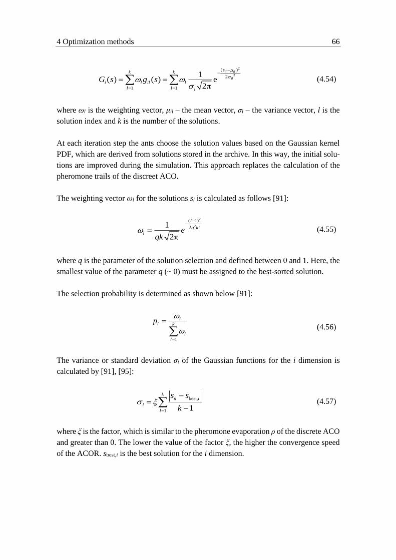
4 Optimization methods 66
2
2
( )
2
1 1
1( ) ( ) e
2π
il il
il
sk k
i l il l
l l i
G s g s
(4.54)
where ωl is the weighting vector, μil – the mean vector, σl – the variance vector, l is the
solution index and k is the number of the solutions.
At each iteration step the ants choose the solution values based on the Gaussian kernel
PDF, which are derived from solutions stored in the archive. In this way, the initial solu-
tions are improved during the simulation. This approach replaces the calculation of the
pheromone trails of the discreet ACO.
The weighting vector ωl for the solutions sl is calculated as follows [91]:
2
2 2
( 1)
21
2π
l
q k
l eqk
(4.55)
where q is the parameter of the solution selection and defined between 0 and 1. Here, the
smallest value of the parameter q (~ 0) must be assigned to the best-sorted solution.
The selection probability is determined as shown below [91]:
1
ll k
l
l
p
(4.56)
The variance or standard deviation σi of the Gaussian functions for the i dimension is
calculated by [91], [95]:
best,
1 1
kil i
i
l
s s
k
(4.57)
where ξ is the factor, which is similar to the pheromone evaporation ρ of the discrete ACO
and greater than 0. The lower the value of the factor ξ, the higher the convergence speed
of the ACOR. sbest,i is the best solution for the i dimension.

4 Optimization methods 67
4.5.1.2 Ant Colony Optimization algorithm with the Prospect Theory for continu-
ous domain
Another often used modification of the ACO for the continuous domain is the so-called
Ant Colony Optimization with the Prospect Theory (ACOR-PT). In contrast to the ACOR,
the search of the optimal solution by the ACOR-PT is based on the prospect theory (PT)
instead of the Gaussian distribution function. The PT describes making human decisions
in high-risk situations such as lotteries. This theory was introduced by D. Kahneman and
A. Tversky in 1979. [96]
In the ACOR-PT, the solutions are chosen not only based on the probability weighting
function, but also on an objective function of the optimization problem. For this purpose,
the mean of the objective function of all solutions stored in the archive, the so-called
reference point, is determined using equation (4.40). It determines whether the established
solutions for the objective function belong to gains or losses. Based on this reference
point, a value function for the gains or losses can be built as shown in Figure 4.7.
Figure 4.7 Value function [92]
Value function
Prospect
Gains
Losses
Reference point

4 Optimization methods 68
If the calculated solution is greater than the reference point, it is in the gain area. If the
solution is less than the reference point, it is in the loss area.
The value function v(sl) of the PT is determined as shown in equation (4.58):
, 0( )
( ) , 0
l l
l
l l
s sv s
s s
(4.58)
where α, β, λ are the constant parameters, which are greater than 0 and must be defined
dependent on the optimization problem. The general recommendation for the parameter
values in the literature [92], [97] is α=β=0.88 and λ=2.25.
In the ACOR-PT the best solution is determined using the probability weighting function
ω(pl), which is calculated according to the following equation:
1( )
( (1 ) )
ll
l l
pp
p p
(4.59)
where γ is the weighting parameter, which is defined between 0.61 and 0.69 [97].
The probability pl is calculated utilizing equation (4.56) but with the only difference that
k is the number of the solutions, which are stored in the archive. In addition, the weighting
vector ωl is determined using equation (4.55).
Based on the value function v(sl) and probability weighting function ω(pl), the so-called
probabilistic prospect V(sl) for choosing the solution sl is established by:
( ) ( ) ( )l l lV s v s p (4.60)
In the ACOR-PT the best solution must have the greatest prospect value. This best solu-
tion is used to create a new ant colony in each iteration step as follows:
best 0,1l ls s N (4.61)
where Nl(0,1) is the standard Gaussian distribution with the mean 0 and variance 1.

4 Optimization methods 69
4.5.2 Performance
The ACO is a quite new optimization technique, which was developed in the early 1990’s.
Nevertheless, it is already utilized in many different fields for solving optimization prob-
lems. There are some main advantages, which make the ACO attractive for the us-
ers [92], [94]:
It finds an effective solution in a very large solution space.
It is very flexible also by dynamic and complex optimization problems.
It can be used for broad applications.
It usually has a low computation time.
Nevertheless, the ACO has some disadvantages, which should be considered by choosing
an optimization method:
Its result is strongly dependent on the choice of its parameter values.
Its convergence is ensured. However, the computation time sometimes can be long.
It sometimes needs additional methods to find a local minimum.
4.5.3 Non-linear redispatch optimization problem for the ACO
The fitness function and constraints of the redispatch optimization problem for the ACO
are already described in detail in chapter 4.2.5.
4.5.4 Algorithm adaptation for the non-linear redispatch optimization
problem
The ACO is developed and adapted for the introduced redispatch optimization problem
to compare its results with the results of the remaining optimization techniques, which
are utilized in this work. In addition, it is also tested in the small network model and
simplified network model of the ENTSO-E power grid (see chapter 5.1).

4 Optimization methods 70
The ants of the ACO consist of possible power generation changes for all power plant
combinations and binary status values for the start-up and shut-down. Furthermore, the
positive and negative redispatch potentials of each power plant pair must be considered
as well as by using the GA, MVMO or PSO.
To solve the previously introduced optimization problem for the redispatch realization
the ACOR-PT is chosen in this work.
At the beginning of the simulation, the initial colony is randomly created. Then the
weighting vector, selection probability and probability weighting function are calculated
using equations (4.55), (4.56) and (4.59). After that the reference point, which is the mean
of the objective function, is determined by equation (4.40). It is utilized to calculate the
value function and probabilistic prospect by equations (4.58) and (4.60). The best solution
has the greatest probabilistic prospect value. It is used to calculate the standard deviation
of the Gaussian functions and create a new ant colony in each iteration step resp. by equa-
tions (4.56) and (4.61). This iterative process repeats until the break conditions are ful-
filled. The developed ACOR-PT is described in detail in chapter 4.5.1.2.
The developed ACOR-PT for the considered redispatch optimization problem is param-
eterized as follows:
The ant colony consists of 400 individuals, which include 150 additional active
ants.
The parameter of the solution selection q is 0.5.
The weighting parameter γ is 0.68.
The constant parameters α=β and λ resp. are equal to 0.88 and 2.0.
The factor ξ is 0.875.
The iteration number is 1000. However, if the best solution cannot be improved
many iterations, the iterative process is stopped.
The maximum number of runs is 10.
The static penalty for the constraint handling is 1000000.

71
5 Case study
The optimization techniques for the redispatch optimization problem, which are intro-
duced in chapter 4, are programmed in the MATLAB computing environment. The de-
veloped algorithms are able to find the optimal solutions for the cost objective functions
by equation (4.6) and (4.35) taking into account the previously formulated linear and non-
linear constraints for redispatch realization by equation (4.9), (4.11), (4.12), (4.33),
(4.34), (4.36), (4.37).
5.1 Test network models
The MATLAB routines are tested with the help of a simple small network model and
simplified network model of the ENTSO-E power grid.
5.1.1 Small network model
The small test network model, which is utilized to verify the introduced optimization
methods, is shown in Figure 5.1 and consists of the following elements:
8 bus bars
8 power plants
10 power lines
load on bus bar ‘N6’
All power lines have the same parameters to simplify the verification of the simulation
results.
Therefore, this test grid model allows to easily understand and manually verify the opti-
mal solutions of the cost optimization problems, which are suggested by the considered
optimization techniques.

5 Case study 72
N5
G G
G G
N1 N2
N4
L1
L2 L3 L8
G
G
G
G
N3
N6
N7 N8
L5 L7
L9
L4 L6 L10
Figure 5.1 Small test network model
To analyze the effectiveness of the developed optimization algorithms, an average cost
scenario for the power plant cycling costs and levelized costs of electricity, which is based
on the data from Table 3.1, Table 3.2 and Table 3.3, and the congestions on line ‘L5’ and
‘L7’ in the small test network model are chosen for this work. The costs for realization of
the active power changes and sensitivity coefficients of lines ‘L5’ and ‘L7’ are introduced
in Table 5.1.
Table 5.1 Average cost scenario and sensitivity coefficients of lines ‘L2’ and ‘L5’
Power plant bus bar N1 N2 N3 N4 N5 N6 N7 N8
Costs in €/MWh 50 80 50 100 220 190 120 50
Sensitivity coefficients
of the line ‘L5’ 0.588 0.66 0.5017 0.445 -0.055 0.017 0.16 0.088
Sensitivity coefficients
of the line ‘L7’ 0.653 0.663 0.635 0.611 0.721 -0.054 0.527 0.245
5.1.2 Simplified ENTSO-E network model
As already mentioned, a simplified grid model of the ENTSO-E area is used to verify the
developed optimization methodologies. This model is based on the results of the
‘DynaGridCenter‘ research project funded by the Federal Ministry for Economic Affairs
and Energy in Germany [98]. In this project, the developed test network model represents
the entire ENTSO-E transmission system. Furthermore, it is based on a cluster model,
which is generated within the EU e-Highway2050 project [99]. Here, EU areas with sim-
ilar characteristics such as the population or installed wind power are combined in clus-
ters (Figure 5.2).

5 Case study 73
Figure 5.2 Cluster model of the e-Highway2050 project [99]
Due to the strong integration of the renewable energy sources (RES) in Germany and its
central location, the German transmission network is modeled more detailed in the
‘DynaGridCenter‘ project. Therefore, each cluster in Germany is represented by 3 bus
bars, i.e. the German transmission system consists of 21 bus bars. Other countries or areas
are modeled by only one bus bar.
Hence, the developed network model includes in total 34 bus bars: 21 bus bars for Ger-
many and 13 for the remaining ENTSO-E areas. These bus bars are connected by 168
transmission lines of the 380 kV voltage level. A network topology of the grid model is
shown in Figure 5.3.

5 Case study 74
Figure 5.3 Simplified ENTSO-E network model [98]
Furthermore, the conventional power plant, RES, which are modeled by a positive load,
and consumption are connected to each bus bar in the power grid model (Figure 5.4).
G
RES
Figure 5.4 Bus bar model [98]

5 Case study 75
5.2 Redispatch optimization without considering the power
plant cycling costs
First of all, the optimization methodologies are verified in the previously introduced small
network model and simplified network model of the ENTSO-E power grid. Here, the
simplex solves the linear redispatch optimization problem without taking into account the
PPCC, which is described in detail in chapter 4.1.2. The metaheuristic methods solve the
same optimization problem, however, with the non-linear power flow equations, which
is described in chapter 4.2.5.
5.2.1 Simulation results in the small network model
Firstly, all optimization techniques developed in this work are tested in the simple small
network model, which is described in detail in chapter 5.1.1 and shown on Figure 5.1.
5.2.1.1 Single network line congestion
In the small network model there are a load of 2500 MW at bus bar ‘N6’ and a power
plant at each bus bar with a rated active power of 500 MW. All power plants can be
completely shut down, i.e. the power generation in this case is equal to 0.
According to the merit order the power plants at bus bars ‘N1’, ‘N2’, ‘N3’, ‘N4’ and ‘N8’
are working with their rated power to cover the load consumption. Hence, there is still a
redispatch potential of maximum 1500 MW in the network model.
Furthermore, in this work, different cost scenarios are created based on the data from Ta-
ble 3.1. Here, a variety of the LCOE for real conventional power plant types, from small-
est to greatest values, are used.
To analyze the effectiveness of the developed optimization algorithms for the redispatch
optimization without considering the PPCC, an average cost scenario and the single con-
gestion of 346.5 MW on line ‘L5’ are chosen (see Table 5.1).

5 Case study 76
If the constraints for the considered optimization problem include the sensitivity coeffi-
cients of line ‘L5’, rated active powers of all power plants and their positive and negative
redispatch potentials, this optimization problem is becoming linear. Therefore, it can be
solved by the simplex algorithm, which could be faster than the metaheuristic methods.
Table 5.2 represents the simulation results of the developed optimization methods for the
already mentioned single congestion of 346.5 MW on line ‘L5’ taking into account only
the linear constraints without considering the PPCC. Moreover, the simulation time is
mean value, which is based on the computation time from twenty simulations for each
optimization method.
Table 5.2 Simulation results for the single congestion of 346.5 MW on line ‘L5’ taking into
account only the linear constraints
Simulation results Optimization methods
Simplex GA MVMO PSO ACO
Simulation time in s 0.011 2.59 10.386 3.392 3.24
Congestion power deviation
on line ‘L5’ in MW 4.2 4.2 4.2 4.2 4.2
Power plants (start-up) 6 and 7 6 and 7 6 and 7 6 and 7 6 and 7
Power plants (drive down) 2 and 4 2 and 4 2 and 4 2 and 4 2 and 4
Active power changes
in MW for start-up
208.37 and
500
208.37 and
500
208.37 and
500
208.37 and
500
208.37 and
500
Active power changes
in MW for driving down
500 and
208.37
500 and
208.37
500 and
208.37
500 and
208.37
500 and
208.37
Total costs in €/h 38753.39 38753.39 38753.39 38753.39 38753.39
In this case, all considered optimization algorithms provide identical results. As expected,
the simulation time of the simplex is the shortest one in comparison to the introduced
metaheuristic methods. Furthermore, the MVMO needs significantly more computation
time. Nevertheless, based on the simulation results, the GA, PSO and ACO solve the
redispatch optimization problem fast enough.
In this scenario, only the power plants at bus bars ‘N5’, ‘N6’ and ‘N7’ can be started-up.
Furthermore, the power plants at bus bars ‘N1’, ‘N2’, ‘N3’, ‘N4’ and ‘N8’ can be driven
down. Here, the best optimal solution is the utilization of the power plants at bus bars
‘N2’, ‘N4’, ‘N6’ and ‘N7’ due to their high sensitivity coefficients and the less total costs
for the redispatch realization. Firstly, the capacity of the power plants at bus bars ‘N2‘
and ‘N7’ is completely exhausted. However, the power plants at bus bars ‘N4’ and ‘N6’
need to be utilized as well because the capacity of the first power plant pair is not enough
to remedy the occurred line congestion.

5 Case study 77
However, the linearization of the power flow function can lead to some deviations in the
line congestion calculations, especially in the highly loaded power grids. In this scenario,
there is a deviation of the congestion power calculation of 4.2 MW. Therefore, in the next
step, the SS, which is described in detail in chapter 4.1.3, is used to remedy this conges-
tion deviation. Based on the simulation results, the deviation of 4.2 MW is completely
remedied and an average simulation time of the SS is only 0.324 s.
In addition, the non-linear power flow equations are included into the previously intro-
duced linear optimization problem instead of the network sensitivity analysis.
Table 5.3 represents the simulation result for the same congestion on line ‘L5’ but using
the non-linear load flow function for the redispatch problem constraints.
Table 5.3 Simulation results for the single congestion of 346.5 MW on line ‘L5’ taking into
account the non-linear load flow function
Simulation results Optimization methods
GA MVMO PSO ACO
Simulation time in s 391.48 442.38 378.41 338.43
Power plants (start-up) 6 and 7 6 and 7 6 and 7 6 and 7
Power plants (drive down) 2 and 4 2 and 4 2 and 4 2 and 4
Active power changes
in MW for start-up
199.17 and
500
199.17 and
500
199.17 and
500
199.17 and
500
Active power changes
in MW for driving down
500 and
199.17
500 and
199.17
500 and
199.17
500 and
199.17
Total costs in €/h 37925.30 38753.30 38753.30 38753.30
Here, all introduced metaheuristic methodologies have a large computation time. The op-
timal solution is using the same power plants as well. However, the needed power gener-
ation changes, resp. the total costs, are less than in the first scenario. Hence, in the previ-
ous test case there is a deviation of 2.18% or 828.09€/h from the optimal total costs of
37925.30 €/h.
5.2.1.2 Multiple network line congestion
Furthermore, the developed optimization algorithms are verified through the simulation
of multiple network line congestions in the small grid model. The initial conditions of this
test network model are described in chapter 5.2.1.1. In addition, an average cost scenario,

5 Case study 78
which is already used in chapter 5.2.1.1, and the multiple congestion of 346.5 MW and
300 MW on lines ‘L5’ and ‘L7’ are considered (see Table 5.1).
Table 5.4 represents the simulation results of the developed optimization methods for the
multiple line congestion taking into account only the linear constraints for the redispatch-
ing.
Table 5.4 Simulation results for the multiple congestion on lines ‘L5’ and ‘L7’ taking into
account only the linear constraints
Simulation results Optimization methods
Simplex GA MVMO PSO ACO
Simulation time in s 0.018 4.09 9.46 3.70 3.11
Congestion power deviation
on line ‘L5’ in MW 6.3 6.3 6.3 6.3 6.3
Congestion power deviation
on line ‘L7’ in MW 18 18 18 18 18
Power plants (start-up) 6 and 7 6 and 7 6 and 7 6 and 7 6 and 7
Power plants (drive down) 2 and 4 2 and 4 2 and 4 2 and 4 2 and 4
Active power changes
in MW for start-up
378.20 and
402.38
378.20 and
402.38
378.20 and
402.38
378.20 and
402.38
378.20 and
402.38
Active power changes
in MW for driving down
280.58 and
500
280.58 and
500
280.58 and
500
280.58 and
500
280.58 and
500
Total costs in €/h 47697.58 47697.58 47697.58 47697.58 47697.58
In this scenario, all optimization methods provide identical results as well as in the previ-
ous test case. As expected, the simplex has the shortest computation time.
Here, the best optimal solution is the utilization of the power plants at bus bars ‘N2’, ‘N4’,
‘N6’ and ‘N7’ due to their high sensitivity coefficients and the less total costs for the
redispatch realization.
Furthermore, there are deviations of the congestion power calculation of 6 MW and
18 MW on lines ‘L5’ and ‘L7’. Therefore, the non-linear power flow function is included
into the linear optimization problem instead of the network sensitivity analysis.
Table 5.5 represents the simulation results for the multiple line congestion using the non-
linear power flow equations for the constraints of the redispatch problem.

5 Case study 79
Table 5.5 Simulation results for the multiple congestion on lines ‘L5’ and ‘L7’ taking into
account the non-linear load flow function
Simulation results Optimization methods
GA MVMO PSO ACO
Simulation time in s 457.56 517.09 394.87 363.58
Power plants (start-up) 6 and 7 6 and 7 6 and 7 6 and 7
Power plants (drive down) 2 and 4 2 and 4 2 and 4 2 and 4
Active power changes
in MW for start-up
416.15 and
339.97
416.15 and
339.97
416.15 and
339.97
416.15 and
339.97
Active power changes
in MW for driving down
256.21 and
500
256.21 and
500
256.21 and
500
256.21 and
500
Total costs in €/h 49378.91 49378.91 49378.91 49378.91
In this scenario, the metaheuristic methods have again a large computation time. The op-
timal solution is using the same power plants as well as in the linear redispatch optimiza-
tion problem. However, to remedy the multiple line congestion completely, the power
generation changes, resp. the total costs, must be greater than it is calculated in the previ-
ous test case. Moreover, there is a deviation of 3.4% or 1681.33€/h from the optimal
solution with the total costs of 49378.91€/h.
5.2.2 Simulation results in the simplified ENTSO-E network model
The considered optimization methodologies are also verified through simulations of mul-
tiple network line congestions in the network model of the ENTSO-E area as well, which
is described in detail in chapter 5.1.2 and shown on Figure 5.3.
5.2.2.1 Multiple network line congestion
In this case study, the redispatch can be realized by the utilization of the power plants in
the entire ENTSO-E area. This area is represented by 34 bus bars. There is a power plant
on each node. Furthermore, there is a power transit of 6 GW from north to south of Ger-
many. According to the merit order the power plants at bus bars ‘1’, ‘2’, ‘4’, ‘5’, ‘7’, ‘9’,
‘11’, ‘12’, ‘13’, ‘14’, ‘15’, ‘17’, ‘18’, ‘20’ and ‘21’ (see Figure 5.3) are working with their
rated power to cover the load consumption in Germany. These power plants can be com-
pletely shut down, i.e. their power generation is equal to 0.

5 Case study 80
The positive and negative redispatch potentials of the power plants in Germany, which
are used in this scenario, are shown in Table 5.6. The remaining power plants in other
countries have the positive redispatch potentials of 2000 MW and costs for the redispatch
realization of 110 €/MWh each.
Table 5.6 Positive and negative redispatch potentials in Germany
Power plant bus bar 1 2 3 4 5 6 7 8 9 10
Positive redispatch
potential in GW 0 0 1.2 0 0 1.2 0 2 0 0.5
Negative redispatch
potential in GW 2.8 2.8 0 3 3 0 5.3 0 1 1
Power plant bus bar 12 13 14 15 16 17 18 19 20 21
Positive redispatch
potential in GW 0 0 0 0 0.4 0 0 0.8 0 0
Negative redispatch
potential in GW 1 1 1 1 0 1 1 0 1.8 1.8
In this work, different cost scenarios are created based on the data from Table 3.1. Here,
a variety of the levelized costs of electricity for real conventional power plant types, from
minimum to maximum value, are used. To analyze the effectiveness of the developed
optimization techniques, the average cost scenario, which is shown in Table 5.7, and the
multiple congestion of 104 MW, 118 MW and 63 MW resp. on the double power lines
between bus bars ‘1’ and ‘2’, ‘1’ and ‘3’, ‘11’ and ‘19’ are chosen. Therefore, the con-
straints for the linear redispatch optimization problem include the sensitivity coefficients
of these three power lines (Table 7.1), rated active powers of all power plants and their
positive and negative redispatch potentials (Table 5.6).
Table 5.7 Average cost scenario
Power plant bus bar 1 2 3 4 5 6 7
Costs in €/MWh 50 55 110 50 60 120 50
Power plant bus bar 8 9 10 11 12 13 14
Costs in €/MWh 140 50 110 80 70 60 50
Power plant bus bar 15 16 17 18 19 20 21
Costs in €/MWh 45 130 90 65 155 85 60
Table 5.8 represents the simulation results of the developed optimization techniques for
the already described multiple line congestion taking into account only the linear con-
straints without considering the PPCC.

5 Case study 81
Table 5.8 Simulation results for the multiple congestion on line between bus bars ‘1’ and ‘2’,
‘1’ and ‘3’, ‘11’ and ‘19’ taking into account only the linear constraints
Simulation results Optimization methods
Simplex GA MVMO PSO ACO
Simulation time in s 0.047 102.42 178.57 157.24 105.75
Congestion power deviation on
line between ‘1’ and ‘2’in MW 3.1 3.1 3.1 3.1 3.1
Congestion power deviation on
line between ‘1’ and ‘3’in MW
6.4 6.4 6.4 6.4 6.4
Congestion power deviation on
line between ‘11’ and ‘19’
4.5 4.5 4.5 4.5 4.5
Power plants (start-up) 3, 16 and
19
3, 16 and
19
3, 16 and
19
3, 16 and
19
3, 16 and
19
Power plants (drive down) 1 1 1 1 1
Active power changes
in MW for start-up
178.74,
292.03 and
133.93
178.74,
292.03 and
133.93
178.74,
292.03 and
133.93
178.74,
292.03 and
133.93
178.74,
292.03 and
133.93
Active power changes
in MW for driving down 604.69 604.69 604.69 604.69 604.69
Total costs in €/h 48148.89 48148.89 48148.89 48148.89 48148.89
The optimization methodologies provide identical results as well as in the previous sce-
narios. The simplex method also has the shortest computation time compare to the me-
taheuristic techniques.
In this test case, the best optimal solution is the utilization of the power plants at bus bars
‘1’, ‚3‘, ‘16’ and ‘19’ due to their high sensitivity coefficients and less total costs for the
redispatch realization.
In addition, there are deviations of the congestion power calculation of 3.1 MW, 6.4 MW
and 4.5 MW on lines between bus bars ‘1’ and ‘2’, ‘1’ and ‘3’, ‘11’ and ‘19’. Therefore,
in the next step, the non-linear power flow equations are included into the previously
introduced linear optimization problem instead of the network sensitivity analysis as well.
Table 5.9 represents the simulation result for the mentioned multiple line congestion but
using the non-linear load flow function for the constraints.
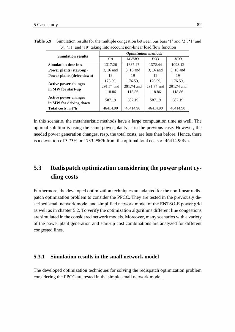
5 Case study 82
Table 5.9 Simulation results for the multiple congestion between bus bars ‘1’ and ‘2’, ‘1’ and
‘3’, ‘11’ and ‘19’ taking into account non-linear load flow function
Simulation results Optimization methods
GA MVMO PSO ACO
Simulation time in s 1317.26 1687.47 1372.44 1098.12
Power plants (start-up) 3, 16 and 3, 16 and 3, 16 and 3, 16 and
Power plants (drive down) 19 19 19 19
Active power changes
in MW for start-up
176.59,
291.74 and
118.86
176.59,
291.74 and
118.86
176.59,
291.74 and
118.86
176.59,
291.74 and
118.86
Active power changes
in MW for driving down 587.19 587.19 587.19 587.19
Total costs in €/h 46414.90 46414.90 46414.90 46414.90
In this scenario, the metaheuristic methods have a large computation time as well. The
optimal solution is using the same power plants as in the previous case. However, the
needed power generation changes, resp. the total costs, are less than before. Hence, there
is a deviation of 3.73% or 1733.99€/h from the optimal total costs of 46414.90€/h.
5.3 Redispatch optimization considering the power plant cy-
cling costs
Furthermore, the developed optimization techniques are adapted for the non-linear redis-
patch optimization problem to consider the PPCC. They are tested in the previously de-
scribed small network model and simplified network model of the ENTSO-E power grid
as well as in chapter 5.2. To verify the optimization algorithms different line congestions
are simulated in the considered network models. Moreover, many scenarios with a variety
of the power plant generation and start-up cost combinations are analyzed for different
congested lines.
5.3.1 Simulation results in the small network model
The developed optimization techniques for solving the redispatch optimization problem
considering the PPCC are tested in the simple small network model.

5 Case study 83
Due to the significant low costs, which need to be spent for the power plant start-up, in
comparison with the costs for the power plant generation changes, the start-up costs can
only have a sufficient influence on the total costs in some rare cases. For example, if the
generation changes to remedy a congestion are low or the power plants have similar im-
pact on the line power flow due to similar generation prices etc. Only in these cases, the
start-up costs might make a rather large part of the total costs spending for the redispatch
realization.
Furthermore, in the introduced redispatch optimization problem the costs for the power
plant generation changes are considered in euros per megawatt hour. Hence, these calcu-
lated total costs are spent only for an hour of the redispatching. However, most of con-
gestions take many hours. At the same time, the start-up of power plants is realized only
once during a redispatch, i.e. the start-up costs must be spent only once for each power
plant.
Therefore, a special test case is considered to verify the developed optimization algo-
rithms with the binary variables for taking into account the PPCC. The initial conditions
of the test grid model are taken from chapter 5.2.1.1. There is the single congestion of
30 MW on line ‘L5’. Furthermore, another cost scenario, which is based on the data
from Table 3.1, is created for testing. The merit order remains the same power plants as
well as in the test case from chapter 5.2.1.1. All chosen LCOE refer to the coal-fired
power plant type. This power plant type is selected because the total PPCC, resp. the start-
up costs, are highest for the coal-fired power plants (see Table 3.2 and Table 3.3). In
addition, it is assumed that the considered line congestion is remedied for one hour.
Furthermore, the power plant shut-down costs are neglected for the simulations because
they are very small compare to another cost types (see Table 3.4).
The costs for the realization of the start-up and active power changes are introduced in Ta-
ble 5.10.
Table 5.10 Special cost scenario of the LCOE and PPCC
Power plant bus bars N1 N2 N3 N4 N5 N6 N7 N8
LCOE in €/MWh 50 60 50 70 90 85 100 50
PPCC in € - - - - 45 250 70 -
Firstly, the redispatch optimization problem includes the sensitivity analysis, rated active
powers of all power plants, their positive and negative redispatch potentials and PPCC.
Here, the binary variables of the PPCC makes the optimization problem non-linear.

5 Case study 84
Therefore, the simplex is incapable of solving it. However, the metaheuristic methodolo-
gies can be utilized for this task.
Table 5.11 represents the simulation results of the optimization methods for the already
mentioned single congestion on line ‘L5’ considering the sensitivity analysis and PPCC.
Table 5.11 Simulation results for the single congestion of 30 MW on line ‘L5’ taking into ac-
count the sensitivity analysis and PPCC
Simulation results Optimization methods
GA MVMO PSO ACO
Simulation time in s 11.36 15.82 10.30 9.11
Congestion power deviation
on line ‘L5’ in MW 0.9 0.9 0.9 0.9
Power plants (start-up) 5 5 5 5
Power plants (drive down) 4 4 4 4
Active power changes in MW 60 60 60 60
Total costs in €/h 1245 1245 1245 1245
The optimization methods taking into account the PPCC provide identical results. The
ACO has the shortest simulation time and the MVMO – the longest one.
If the PPCC were not considered in this scenario, the optimal solution for the linear re-
dispatch optimization problem were the selection of the power plants at bus bars ‘N4’ and
‘N6’. Furthermore, the total costs for the redispatch realization were 1051.40 €/h.
However, if the PPCC are considered, the optimal solution is the selection of the power
plants at bus bars ‘N4’ and ‘N5’. Here, the total costs for the redispatching are 1245 €/h.
If the optimal solution were still the selection of the power plants at bus bars ‘N4’ and
‘N6’, the total costs for the redispatch realization were 1301.40 €/h. Therefore, there is a
deviation of 4.53% or 56.40€/h from the optimal total costs.
In the next step, the non-linear power flow equations are included into the redispatch
optimization problem instead of the network sensitivity analysis.
Table 5.12 represents the simulation results of the developed metaheuristic optimization
methods for the single congestion on line ‘L5’ taking into account the non-linear power
flow function and PPCC.

5 Case study 85
Table 5.12 Simulation results for the single congestion of 30 MW on line ‘L5’ taking into ac-
count the non-linear power flow equations and PPCC
Simulation results Optimization methods
GA MVMO PSO ACO
Simulation time in s 609.94 773.71 634.12 534.08
Power plants (start-up) 5 5 5 5
Power plants (drive down) 4 4 4 4
Active power changes in MW 58.15 58.15 58.15 58.15
Total costs in €/h 1208.06 1208.06 1208.06 1208.06
In this simple test case, all introduced optimization algorithms provide identical results
and have a large computation time. Here, the computation time of the ACO is the shortest
one in comparison to other considered metaheuristic methods.
If the PPCC were not considered, the optimal solution were the selection of the power
plants at bus bars ‘N4’ and ‘N6’ as well as in the previous case. Moreover, the total costs
for the redispatch realization were only 969.18 €/h.
However, if the PPCC are considered in the optimization problem, the optimal solution
for the redispatch realization is the selection of the power plants at bus bars ‘N4’ and
‘N5’. In addition, the total costs are 1208.06€/h. If the optimal solution were still the
selection of the power plants at bus bars ‘N4’ and ‘N6’, the total costs for the redispatch
realization were 1219.18 €/h. Therefore, there is a deviation of 0.92% or 11.12€/h from
the optimal solution.
Moreover, the needed power generation changes to remedy the congestion, resp. the total
costs, are less than in the case with the consideration of the sensitivity analysis. Therefore,
there is a deviation of 3.06% or 36.94€/h from the optimal total costs of 1208.06 €/h.
5.3.2 Simulation results in the simplified ENTSO-E network model
The optimization methods for solving the non-linear redispatch optimization problem
considering the PPCC are tested in the simplified network model of the ENTSO-E area
as well.
As already mentioned above, the start-up costs are significantly low than the costs for the
power plant generation changes. Therefore, in most cases they have no influence on the

5 Case study 86
total costs for the redispatch realization and can be neglected. Nevertheless, there are
some rare cases when they can play a major role.
In this work, such seldom case is considered to verify the developed optimization algo-
rithms. The initial conditions of the test grid model are taken from chapter 5.2.2. Further-
more, there is the single congestion only of 20 MW on the double power line between
bus bars ‘1’ and ‘2’. The sensitivity coefficients of this congested power line are given in
Table 7.1. In addition, the cost scenario from chapter 5.2.2 is utilized here as well. How-
ever, the LCOE of the power plant at bus bar ‘8’ are changed to 110 €/MWh.
The chosen LCOE refer to the coal-fired power plant type because its start-up costs are
highest compared to other power plant types (Table 3.2 and Table 3.3). Moreover, it is
assumed that the considered line congestion is remedied for one hour.
In addition, the PPSDC are neglected for the simulations as well as in chapter 5.3.1.
The costs for the realization of the power plant start-up are introduced in Table 5.13.
Table 5.13 Start-up costs for the scenario in the simplified ENTSO-E network model
Power plant bus bar 1 2 3 4 5 6 7
PPCC in € - - 50 - - 95 -
Power plant bus bar 8 9 10 11 12 13 14
Costs in €/MWh 250 0 80 0 0 0 0
Power plant bus bar 15 16 17 18 19 20 21
Costs in €/MWh 0 75 0 0 105 0 0
In this case, the redispatch optimization problem includes the non-linear power flow func-
tion, rated active powers of all power plants, their positive and negative redispatch poten-
tials and PPCC.
Table 5.14 represents the simulation results of the metaheuristic optimization methods for
the single congestion of 20 MW on the double power line between the bus bars ‘1’ and
‘2’ taking into account the non-linear optimization problem.

5 Case study 87
Table 5.14 Simulation results for the single congestion of 20 MW on the power line between
the bus bars ‘1’ and ‘2’ taking into account the non-linear power flow equations and PPCC
Simulation results Optimization methods
GA MVMO PSO ACO
Simulation time in s 2120.85 2715.46 1962.6 1443.61
Power plants (start-up) 3 3 3 3
Power plants (drive down) 1 1 1 1
Active power changes in MW 132.04 132.04 132.04 132.04
Total costs in €/h 710.22 710.22 710.22 710.22
The metaheuristic optimization algorithms provide identical results and have a large com-
putation time. Here, the computation time of the ACO is shortest one in comparison to
other considered metaheuristic methods. Moreover, the MVMO is the slowest algorithm
from the introduced methods.
If the PPCC were not considered in this scenario, the optimal solution were the selection
of the power plants at bus bars ‘1’ and ‘8’. Moreover, the total costs for the redispatch
realization were 505.06 €/h.
However, if the PPCC are considered, the optimal solution is the selection of the power
plants at bus bars ‘1’ and ‘3’. Here, the total costs for the redispatch are 710.22 €/h. If the
optimal solution were still the selection of the power plants at bus bars ‘1’ and ‘8’, the
total costs were 755.06 €/h. Therefore, there is a deviation of 6.31% or 44.84€/h from the
optimal total costs.
In addition, the optimal solution for the non-linear redispatch optimization problem is
exactly the same as for the optimization problem with the network sensitivity analysis
due to the linearization of the power flow equations for the double power line between
the bus bars ‘1’ and ‘2’ in the simplified network model of the ENTSO-E area has no
deviation at the utilized working point.
5.3.3 Conclusions
Obviously, the simplex algorithm is the fastest introduced optimization method and pro-
vides very accurate results. Nevertheless, it cannot solve the redispatch optimization
problem with the non-linear power flow equations. However, in the case of the redispatch
optimization problem a linearization of the load flow function can lead to large deviations

5 Case study 88
in the calculation of the line congestion amounts, especially in the highly loaded electric
networks.
In most cases, the previously introduced metaheuristic algorithms provide the same re-
sults as well as the simplex method if the optimization problem is linear. However, the
metaheuristic optimization methodologies need significantly more computation time.
Moreover, sometimes they are not able to find the global optimum of the optimization
function. In addition, these methods should be adopted and parameterized for the consid-
ered optimization problem, which is not a trivial issue and can take a lot of time. Never-
theless, the utilization of the non-linear power flow equations increases the accuracy of
the redispatch optimization problem definition and, consequently, improves the optimal
solutions in comparison to the standard simplex. However, the sequential simplex, which
is also very fast, can be utilized to remedy congestion calculation deviations. Therefore,
it delivers the same results as the stochastic optimization methods taking into account the
load flow function.
Furthermore, the consideration of the PPCC can also improve the optimal solutions. But
the PPCC can only have a sufficient influence on the total costs in some rare cases. For
example, if the generation changes to remedy a congestion are low, or the power plants
have similar impact on the line power flow due to similar generation prices. But low line
congestions are usually not relevant in the transmission power grids. Therefore, the PPCC
can be neglected in the redispatch optimization if it is done only for one time step. How-
ever, if the redispatching is considered in the time series, the PPCC and PPSDC can have
significantly more influence on the total costs because the power plants might be started-
up and shut down many times, which strongly increases the total costs.
Finally, the long computation time of the stochastic optimization methods for the non-
linear redispatch optimization problem makes it difficult to use them in the online net-
work operation. Therefore, they are more suitable for an academic research.

89
6 Summary and Outlook
Today, the frequency of the redispatch utilization to remedy line congestions in the power
grids, especially in central Europe, has extremely raised because of the high increase of
the European electricity market. Unfortunately, this process causes high costs for the
transmission network operators, resp. for the end customers. Therefore, an efficient re-
dispatch optimization has become a very important issue for the TSOs.
In this work, different optimization methodologies, which are used for the redispatch op-
timization including the technical and economic aspects, are introduced, implemented,
compared and verified in a simple small network model and simplified network model of
the ENTSO-E power grid.
Obviously, the simplex algorithm is the fastest optimization method and used here to
solve the linear redispatch optimization problem with a linearization of the power flow
function, resp. the network sensitivity analysis, and without taking into account the power
plant cycling costs (PPCC). However, this linearization can lead to strong deviations in
the line congestion calculations, especially in the highly loaded electric networks. Con-
sequently, this might significantly reduce the accuracy of the optimal solutions. Here, the
sequential simplex can be used to remedy the deviations of the standard simplex. But both
simplex algorithms are not able to consider the PPCC.
Therefore, the introduced metaheuristic optimization methodologies (the genetic algo-
rithm, Mean Variance Mapping Optimization, Particle Swarm Optimization and Ant Col-
ony Optimization) are utilized to solve the redispatch optimization problem with the non-
linear load flow equations and PPCC. Based on the simulation results, they all provide
accurate solutions for the redispatch optimization with the linear and non-linear con-
straints (see chapters 5.2 and 5.3). However, the metaheuristic approaches have a big
disadvantage, resp. a long computation time, especially in case of the consideration of the
non-linear power flow function. Furthermore, sometimes they are not able to find the
global optimum of the optimization problem. Moreover, the mentioned stochastic opti-
mization methods should be adopted and parameterized for the considered optimization
problem, which is not a trivial task and can take a long time. Therefore, they are not really
appropriate to use them in the online network operation. Nevertheless, they are well suit-
able for an offline study and academic research.
In addition, consideration of the PPCC can also improve the accuracy of the optimal so-
lutions. However, in case of single time step consideration the start-up costs can have a

6 Summary and Outlook 90
relevant influence on the total costs only if the generation changes to remedy a congestion
are low or the power plants have similar impact on the line power flow due to similar
generation prices. Furthermore, low line congestions are usually not relevant in the trans-
mission electric networks. Hence, the PPCC can be neglected in the redispatch optimiza-
tion if it is done only for a snapshot of the power grid state. However, if the redispatch is
considered in the time series, the PPCC and PPSDC could have significantly more influ-
ence on the total costs because power plants may be started-up and shut down many times.
Finally, different approaches (the Power Flow Decomposition and two AC Power Trans-
fer Distribution Factors methods) for the calculation of the sensitivity analysis are intro-
duced, implemented, compared and verified in several standard IEEE test power grid
models and the already mentioned simplified network model of the ENTSO-E area. Based
on the simulation results, the PFD methodology provides the most accurate approxima-
tions of the non-linear power flow equations in all test cases. Moreover, its maximum
deviation is around 9% in case of an extremely high load in the simplified ENTSO-E grid
model. In case of normal load in this network model, there is no deviation from the load
flow function at the utilized working point at all (see the results from chapter 5.3). There-
fore, the PFD method is chosen for the calculation of the network sensitivity analysis in
the test networks models.
In future works, the economic aspects of the redispatch realization could be considered
in the time series. In this case, the PPCC and PPSDC may be larger share of the total costs
because the power plants could be started-up and shut down many times during the redis-
patching. Furthermore, different RES might be included in this process as well.

91
7 List of references
[1] B. Haller, Versorgungssicherheit in Deutschland, Stuttgart, Germany: Energie
Speicher Symposium, 2013.
[2] C. O. Heyde, Dynamic Voltage Security Assessment for On-Line Control Room
Application, Ph.D. dissertation, Magdeburg, Germany: Otto-von-Guericke
University, 2010.
[3] M. Wolter, Agent based Energy Management Systems, Ph.D. dissertation, Aachen,
Germany: Shaker Verlag, 2012.
[4] "REGULATION (EC) No 714/2009 OF THE EUROPEAN PARLIAMENT AND
OF THE COUNCIL of 13 July 2009," Official Journal of the European Union,
August 2009.
[5] I. Chychykina, C. Klabunde and M. Wolter, "Comparison of different redispatch
optimization strategies," in 2017 IEEE Manchester PowerTech, Manchester,
England, 18-22 June 2017.
[6] J. E. Blank, "Engpassmanagement an grenzüberschreitenden Netzkuppelstellen,"
Kaiserslautern, Germany, 2015.
[7] ENTSO-E, "Continental Europe Operation Handbook. Operational Security," 2004.
[8] "www.bundesnetzagentur.de," [Online]. [Accessed 3 September 2015].
[9] I. Androcec and I. Wangensteen, "Different Methods for Congestion Management
and Risk Management," in 9th International Conference on Probabilistic Methods
Applied to Power Systems, Stockholm, Sweden, June 11-15, 2006.
[10] Federal Ministry for Economic Affairs and Energy in Germany oder
Bundesministerium der Justiz und für Verbraucherschutz in Deutschland, Gesetz
über die Elektrizitäts- und Gasversorgung (Energiewirtschaftsgesetz - EnWG).
[11] Federal Ministry of Justice and Consumer Protection in Germany oder
Bundesministerium der Justiz und für Verbraucherschutz in Deutschland,
Verordnung zur Regelung des Netzanschlusses von Anlagen zur Erzeugung von
elektrischer Energie, (Kraftwerks-Netzanschlussverordnung - KraftNAV), § 7
Netzzugang bei Engpässen, 26.06.2007.
[12] Federal Ministry for Economic Affairs and Energy in Germany oder
Bundesministerium der Justiz und für Verbraucherschutz in Deutschland, Gesetz
über die Elektrizitäts- und Gasversorgung (Energiewirtschaftsgesetz - EnWG).

List of references 92
[13] C. König, Engpassmanagement in der deutschen und europäischen
Elektrizitätsversorgung, Baden-Baden, Germany: Nomos Verlagsgesellschaft,
2013.
[14] "Analysis of cross-border congestion management methods for the EU internal
electricity market," Final report, Study commissioned by the European Commission
Directorate-General Energy and Transport, June 2004.
[15] P. Trojan, M. Wolter and P. Komarnicki, "Agent based power system management
- Concept of congestion management," in IEEE 18th International Scientific
Conference on Electric Power Engineering (EPE), Ostrava, Czech Republic, 03 Juli
2017.
[16] T. Wawer, "Konzepte für ein nationales Engpassmanagement im deutschen
Übertragungsnetz," Zeitschrift für Energiewirtschaft (ZfE), 2007.
[17] I. Chychykina, C. Klabunde and M. Wolter, "Redispatch with power flow
decomposition and power transfer distribution factors methods," in 2016 51st
International Universities Power Engineering Conference (UPEC), Coimbra,
Portugal, 6-9 September 2016.
[18] B. Dieckmann, Engpassmanagement im Europäischen Strommarkt, Ph.D.
dissertation, Münster, Germany: Wilhelms-University Münster, November 2008.
[19] J. Kühling, Die neuen Engpass- Leitlinien der Kommission im grenzüberstehenden
Stromhandel – Freie Fahrt für das Open Market Coupling in Deutschland?, Recht
der Energiewirtschaft: RdE 2006, pp. 173-174, 2006.
[20] ERGEG, Draft Framework Guidelines on Capacity Allocation and Congestion
Management for Electricity, pp. 45, September 2010.
[21] E. Böttcher, Market Coupling in Europa, emw, 2009.
[22] A. R. Bergen and V. Vittal, Power System Analysis, New Jersey, USA: 2nd ed.,
Prentice Hall, pp. 13-14, 2000.
[23] M. Wolter and B. Huehnerbein, "Identification of cross-border power flows in
integrated networks based on the principle of superposition," in IEEE International
Power and Energy Conference, Johor Bahru, Malaysia, 2008.
[24] M. Wolter, "About the impact of burdening and relieving partial power flows
caused by Loop Flows in interconnected networks on ITC amount," in 2009 IEEE
Power & Energy Society General Meeting, Calgary, Canada, 26-30 July 2009.
[25] M. Wolter and B. R. Oswald, "Congestion management and determination of
optimal grid expansion and retreat strategies using a modified Boundary Load Flow
Method," in 2008 40th North American Power Symposium, Calgary, Canada,
September 2008.

List of references 93
[26] M. Wolter and L. Hofmann, "Allocation of responsibility for congestions in
transmission systems based on power flow decomposition," in IASTED AsiaPES
2010, Phuket, Thailand, November 2010.
[27] T. Leveringhaus and L. Hofmann, "Comparison of methods for state prediction:
Power Flow Decomposition (PFD), AC Power Transfer Distribution factors (AC-
PTDFs), and Power Transfer Distribution factors (PTDFs)," in 2014 IEEE PES
Asia-Pacific Power and Energy Engineering Conference (APPEEC), Hong Kong,
China, December 2014.
[28] J. Kumar and A. Kumar, "ACPTDF for Multi-transactions and ATC Determination
in Deregulated Markets," International Journal of Electrical and Computer
Engineering (IJECE), vol. 1, pp. 71-84, September 2011.
[29] Saloni and M. Dhakla, "ATC Determination for Different Transactions Using
ACPTDF," International Journal of Modern Engineering Research (IJMER), vol.
3, pp. 431-435, January 2013.
[30] P. Venkatesh, B. Manikandan, S. C. Raja and A. Srinivasan, Power Systems –
Analysis, Security and Deregulation, New Delhi, India: PHI Learning Private
Limited, 2012.
[31] "http://www.pserc.cornell.edu/matpower/," [Online]. [Accessed 11 Februar 2019].
[32] "http://www.ee.washington.edu/research/pstca/," [Online]. [Accessed 3 September
2015].
[33] Levelized Cost and Levelized Avoided Cost of New Generation Resources in the
Annual Energy Outlook 2018, Tech. Rep., Washington, USA: U.S. Energy
Information Administration, March 2018.
[34] C. Kost and T. Schlegl, Levelized Cost of Electricity - Renewable Energy
Technologies, Tech. Rep., Freiburg, Germany: Fraunhofer Institute for Solar
Energy Systems ISE, March 2018.
[35] U. Nestle and C. Kunz, Studienvergleich: Stromgestehungskosten verschiedener
Erzeugungstechnologien, Tech. Rep., Berlin, Germany: Agentur für Erneuerbare
Energien, 2014.
[36] N. Kumar, P. Besuner, S. Lefton, D. Agan and D. Hilleman, Power plant cycling
costs, Tech Rep., Sunnyvale, California, USA: Intertek APTECH, NREL Technical
Monitor, July 2012.
[37] K. d. Bergh and E. Delarue, Energy Conversion and Management, vol. 97, Elsevier
Ltd, pp. 70-77, April 2015.

List of references 94
[38] Assessment of startup period at coal-fired electric generating units – Revised, U.S.
Environmental Protection Agency, Office of Air and Radiation, Tech Rep.,
November 2014.
[39] H. Spliethoff, Power generation from solid fuels, Berlin, Germany: Springer Berlin
Heidelberg, 2010.
[40] A. J. Wood, B. F. Wollenberg and G. B. Sheblé, Power generation, operation, and
control, New Jersey, USA: John Wiley & Sons, 2014.
[41] M. Silbernagl, M. Huber and R. Brandenberg, "Improving Accuracy and Efficiency
of Start-Up Cost Formulations in MIP Unit Commitment by Modeling Power Plant
Temperatures," IEEE Transactions on Power Systems, vol. 31, pp. 2578-2586, July
2016.
[42] M. Huber and M. Silbernagl, "Modeling Start-Up Times in Unit Commitment by
Limiting Temperature Increase and Heating," in 12th International Conference on
the European Energy Market (EEM), Lisbon, Portugal, May 2015.
[43] W. Jiekang, L. Jun, W. Jixiang and C. Yuanrui, "Stochastic models for optimal
generation production in electricity markets," in International Conference on Power
System Technology, Kunming, China, October 2002.
[44] S. Abbasi and A. Jamehbozorg, "A comprehensive economic optimization plan for
microgrids considering grid interconnection and line congestion," in Technology
2015 IEEE Green Energy and Systems Conference (IGESC), Long Beach, USA,
November 2015.
[45] A. Nogales, E. Centeno and S. Wogrin, Including start-up and shut down
constraints into generation capacity expansion models for liberalized electricity
markets, Vienna, Austria: unpublished, presented at the second international
AAEE/YEEES PhD Day, March 2013.
[46] A. Antoniou and W.-S. Lu, Practical Optimization. Algorithms and Engineering
Applications, New York, USA: Springer, pp. 321-323, 2007.
[47] H. Karloff, Linear Programming, Boston, USA: Springer, pp. 23-48, 1991.
[48] J. Vaidya, "A secure revised simplex algorithm for privacy-preserving linear
programming," in IEEE International Conference on Advanced Information
Networking and Applications (AINA), Bradford, United Kingdom, pp. 347-354,
May 26-29 2009.
[49] D. K. Nadar, "Some Applications of Simplex Method," International Journal of
Engineering Research and Reviews, pp. 60-63, January 2016.

List of references 95
[50] D. Spielman and S.-H. Teng, "Smoothed Analysis of Algorithms: Why the Simplex
Algorithm Usually Takes Polynomial Time," Journal of the ACM, pp. 385-463,
May 2004.
[51] W. Spendley, G. R. Hext and F. R. Himsworth, "Sequential Application of Simplex
Designs in Optimisation and Evolutionary Operation," Technometrics, pp. 441-461,
April 2012.
[52] V. S. Vassiliadis and R. Conejeros, Sequential Simplex Method, Boston, USA:
Springer, 2008.
[53] J. A. Nelder and R. Mead, "A Simplex Method for Function Minimization," The
Computer Journal, vol. 7, pp. 308–313, January 1965.
[54] R. Haupt and S. E. Haupt, Practical Genetic Algorithms, New Jersey, USA: Wiley,
pp. 27-65, 2004.
[55] D. Simon, Evolutionary Optimization Algorithms, New Jersey, USA: Wiley, pp.
44-59, 2013.
[56] K. Weicker, Evolutionäre Algorithmen, Wiesbaden, Germany: Springer Vieweg,
2015.
[57] M. Gen and R. Cheng, Genetic Algorithms and Engineering Optimization, New
Jork, USA: Wiley, pp. 6-9, 2000.
[58] D. Dasgupta and D. R. McGregor, "Short Term Unit Commitment Using Genetic
Algorithms," in International Conference on Tools with Artificial Intelligence,
Boston, Massachusetts, USA, 1993.
[59] A. Popov, Genetic Algorithms for Optimization. Programs for MATLAB, User
Manual, Version 1.0, Hamburg, Germany, 2005.
[60] O. Roeva, "A Modified Genetic Algorithm for a Parameter Identification of
Fermentation Processes," Biotechnology & Biotechnological Equipment, 2006.
[61] M.-C. Popescu, N. E. Mastorakis and L. Popescu-Perescu, "Application of Genetic
Algorithm in Electrical Engineering," International Journal of Pure and Applied
Mathematics, vol. 114, pp. 35-43, May 2017.
[62] Ö. Yeniay, "Penalty Function Methods for Constrained Optimization with Genetic
Algorithms," Mathematical and Computa-tional Applications, vol. 10, pp. 45-56,
2005.
[63] V. Petridis, S. Kazarlis and A. Bakirtzis, "Varying Fitness Functions in Genetic
Algorithm Constrained Optimization: The Cutting Stock and Unit Commitment
Problems," IEEE Transactions on Systems, Man, and Cybernetics, Part B
(Cybernetics), vol. 28, pp. 629- 640, October 1998.

List of references 96
[64] V. Petridis, S. Kazarlis and A. Bakirtzis, "Penalty Function Methods for
Constrained Optimization with Genetic Algorithms: A Statistical Analysis," in
Mexican International Conference on Artificial Intelligence, Yucatan, Mexico, pp
108-117, May 2002..
[65] Z. Michalewicz und M. Schoenauer, „Evolutionary Algorithms for Constrained
Parameter Optimization Problems,“ Evolutionary Computation, Bd. 4, pp. 1- 32,
March 1996.
[66] S. C. Müller, Techno-economic analysis of congestion management in the European
transmission system under consideration of flexibility and uncertainty, Ph.D.
dissertation, Dortmund, Germany: Sierke Verlag, November 2015.
[67] D. Mende, D. S. Stock, T. Hennig, L. Löwer and L. Hofmann, "Multiobjective
Optimization in Congestion Management Considering Technical and Economic
Aspects," in IEEE PES Asia-Pacific Power and Energy Engineering Conference
(APPEEC), Xian, China, October 2016.
[68] J. Abrell, F. Kunz and H. Weigt, "https://mpra.ub.uni-
muenchen.de/65661/1/wp_em_28_Abrell_Kunz_Weigt_Startup.pdf," [Online].
[Accessed 14 Februar 2019].
[69] I. Erlich, G. K. Venayagamoorthy and W. Nakawiro, "A mean-vareance
optimization algorithm," in IEEE Congress on Evolu-tionary Computation,
Barcelona, Spain, pp.1-6, July 2010..
[70] J. L. Rueda, W. H. Guamán, J. C. Cepeda, I. Erlich and A. Vargas, "Hybrid
approach for power system operational planning with smart grid and small-signal
stability enhancement considerations," IEEE Transactions on Smart Grid, vol. 4,
pp. 530-539, March 2013.
[71] I. Erlich, J. L. Rueda, S. Wildenhues and F. Shewarega, "Evaluating the mean-
vareance mapping optimization on the IEEE-CEC 2014 test suite," in 2014 IEEE
Congress on Evolutionary Computation (CEC), Beijing, China, July 2014.
[72] I. Erlich, J. L. Rueda, S. Wildenhues and F. Shewarega, "Solving the IEEE-CEC
2014 expensive optimization test problems by using single-particle MVMO," in
2014 IEEE Congress on Evolutionary Computation (CEC), Beijing, China, July
2014..
[73] J. L. Rueda and I. Erlich, "MVMO for bound constrained single-objective
computationally expensive numerical optimization," in 2015 IEEE Congress on
Evolutionary Computation (CEC), Sendai, Japan, May 2015.
[74] J. L. Rueda and F. Gonzalez-Longatt, "Application of swarm mean-vareance
mapping optimization on location and tuning damp-ing controllers," in 2015 IEEE

List of references 97
Innovative Smart Grid Technologies - Asia (ISGT ASIA), Bangkok, Thailand,
January 2016.
[75] C. J. López-Salgado, O. Añó and D. M. Ojeda-Esteybar, "Joint optimization of
energy and reserve in deregulated power markets: alternative approach using Mean
Vareance Mapping Optimization," in 2016 Power Systems Computation
Conference (PSCC), Genoa, Italy, June 2016.
[76] J. Rueda, A. M. Theologi, M. Ndreko, I. Erlich and P. Palensky, "Metaheuristic
approach for online optimal reactive power management in near-shore wind power
plants," in 2017 IEEE PES Innovative Smart Grid Technologies Conference - Latin
America (ISGT Latin America), Quito, Ecuador, September 2017.
[77] J. Kennedy and R. Eberhart, "Particle swarm optimization," in IEEE International
Conference on Neural Networks, Perth, Australia, December 1995.
[78] K. Y. Lee and J.-B. Park, "Application of Particle Swarm Optimization to Economic
Dispatch Problem: Advantages and Disad-vantages," in 2006 IEEE PES Power
Systems Conference and Exposition, Atlanta, USA, November 2006.
[79] H. Huang, H. Qin, Z. Hao and A. Lim, "Example-based learning particle swarm
optimization for continuous optimization," In-formation Sciences, Nature-Inspired
Collective Intelligence in Theory and Practice, vol. 182, pp. 125-138, January 2012.
[80] V. Karthikeyan, S. Senthilkumar and V. J. Vijayalakshmi, "A New Approach to the
Solution of Economic Dispatch Using Particle Swarm Optimization with Simulated
Annealing," International Journal on Computational Sciences & Applications
(IJCSA), vol. 3, pp. 37-49, June 2013.
[81] X. Wang and X. Qiu, "Application of particle swarm optimization for enhanced
cyclic steam stimulation in an offshore heavy oil reservoir," International Journal
of Information Technology, Modeling and Computing (IJITMC), vol. 1, pp. 37-47,
May 2013.
[82] Y.-S. Cheng, M.-T. Chuang, Y.-H. Liu, S.-C. Wang und Z.-Z. Yang, „A particle
swarm optimization based power dispatch algorithm with roulette wheel re-
distribution mechanism for equality constraint,“ Renewable Energy, Bd. 88, pp. 58-
72, April 2016.
[83] S. Huang and V. Dinavahi, "Multi-group particle swarm optimisation for
transmission expansion planning solution based on LU decomposition," IET
Generation, Transmission & Distribution, vol. 11, May 2017.
[84] P. R. Sujin, T. R. Deva-Prakash and M. M. Linda, "Particle Swarm Optimization
Based Reactive Power Optimization," Journal of Computing, vol. 2, January 2010.

List of references 98
[85] J. C. Bansal, P. K. Singh and M. Saraswat, "Inertia Weight strategies in Particle
Swarm Optimization," in 2011 Third World Congress on Nature and Biologically
Inspired Computing, Salamanca, Spain, October 2011.
[86] J. Xin, G. Chen and Y. Hai, "A Particle Swarm Optimizer with Multi-stage
Linearly-Decreasing Inertia Weight," in 2009 International Joint Conference on
Computational Sciences and Optimization, Sanya, Hainan, China, April 2009.
[87] M. A. Abido, "Optimal design of power-system stabilizers using particle swarm
optimization," IEEE Transactions on Energy Con-version, vol. 17, pp. 406 – 413,
November 2002.
[88] M. Dorigo and T. Stützle, Ant Colony Optimization, Cambridge, Massachusetts,
USA: MIT Press, 2004.
[89] C. Blum, "Ant colony optimization: Introduction and recent trends," Physics of Life
Reviews, pp. 353–373, December 2005.
[90] M. D. Toksari, "Ant colony optimization for finding the global minimum," Applied
Mathematics and Computation, vol. 176, pp. 308–316, May 2006.
[91] C. Blum and C. Socha, "An ant colony optimization algorithm for continuous
optimization: application to feed-forward neural network training," Neural
Computing and Applications, vol. 16, pp. 335–347, March 2007.
[92] C. J. Riadi, Cognitive Ant Colony Optimization: A New Framework in Swarm
Intelligence, Ph.D. dissertation, University of Salford, Manchester, UK, 2014.
[93] M. Dorigo and G. D. Caro, "Ant Colony Optimization: A New Meta-Heuristic," in
1999 IEEE Congress on Evolutionary Computation-CEC99, Washington, USA,
July 1999.
[94] A. Ahuja and A. Pahwa, "Using ant colony optimization for loss minimization in
distribution networks," in the 37th Annual North American Power Symposium,
Ames, USA, October 2005.
[95] P. López-Matencio, "An ACOR-Based Multi-Objective WSN Deployment
Example for Lunar Surveying," Sensors, February 2016.
[96] D. Kahneman and A. Tversky, "Prospect Theory: An Analysis of Decision under
Risk," Econometrica, vol. 47, pp. 263-291, March 1979.
[97] A. Tversky and D. Kahneman, "Advances in prospect theory: Cumulative
representation of uncertainty," Journal of Risk and Uncertainty, vol. 5, pp. 297–
323, October 1992.
[98] DynaGridCenter, Tech. Rep., Nürnberg, Germany, February 2019.
[99] eHighway2050, Country and Cluster installed Capacities, Tech. Rep., 31 March
2015.

99
A Title Annex A
Table 7.1 Sensitivity coefficients of power lines between bus bars ‘1’ and ‘3’, ‘11’ and ‘19’
Power plant bus bar 1 2 3 4 5 6 7
Sensitivity coefficients of line be-
tween bus bars ‘1’ and ‘2’ 0.198 -0.046 0.047 0.106 0.081 0.071 -0.005
Sensitivity coefficients of line be-
tween bus bars ‘1’ and ‘3’ 0.212 0.057 -0.025 0.104 0.071 0.055 0.034
Sensitivity coefficients of line be-
tween bus bars ‘11’ and ‘19’ 0.084 0.072 0.09 0.142 0.172 0.164 0.053
Power plant bus bar 8 9 10 11 12 13 14
Sensitivity coefficients of line be-
tween bus bars ‘1’ and ‘2’ 0 -0.003 0.07 0.035 0.05 0.01 0.011
Sensitivity coefficients of line be-
tween bus bars ‘1’ and ‘3’ 0.034 0.036 0.06 0.038 0.047 0.028 0.03
Sensitivity coefficients of line be-
tween bus bars ‘11’ and ‘19’ 0.04 0.044 0.178 0.236 0.208 0.044 -0.009
Power plant bus bar 15 16 17 18 19 20 21
Sensitivity coefficients of line be-
tween bus bars ‘1’ and ‘2’ 0.005 0.011 0.018 0.018 0.03 0.025 0.027
Sensitivity coefficients of line be-
tween bus bars ‘1’ and ‘3’ 0.034 0.034 0.038 0.038 0.035 0.04 0.038
Sensitivity coefficients of line be-
tween bus bars ‘11’ and ‘19’ 0.021 0.003 0.003 0.003 -0.218 -0.007 -0.024

Published MaFo Books 100
Published MaFo Books
[1] A. Orths: Multikriterielle, optimale Planung von Verteilungsnetzen im
liberalisierten Energiemarkt unter Verwendung von Spieltheoretischen Verfahren,
2003. ISBN: 3-929757-57-5
[2] M. Purmann: Optimierung des Betriebsverhaltens von PEM-Brennstoffzellen unter
Berücksichtigung von elektrischem und Gesamtwirkungsgrad bei unterschiedlichen
Lastanforderungen und Betriebsparametern, 2003. ISBN: 3-929757-63-X
[3] M. Al-Hamid: Extraktion von höheren Moden TEM-Wellenleitern, 2004.
ISBN: 3 929757-64-8
[4] H. Haase, J. Nitsch, T. Steinmetz: Transmission-Line Super Theory – A new
Approach to an Effective Calculation of Electromagnetic Interference, 2004.
ISBN: 3 929757-67-2
[5] A. Bachry: Power Quality Studies in Distribution Systems Involving Spectral
Decomposition, 2004. ISBN: 3-929757-68-0
[6] Z. Styczynski (Editor): Power Network and Renewables – A Scientific Report- (5
Years Research), 2004. ISBN: 3-929757-69-9
[7] E. Blume: Numerische Analyse der Kopplung linearer Antennen innerhalb eines
Resonators, 2004. ISBN: 3-929757-71-1
[8] E. Handschin, Z. Styczynski (Editors): Power System Application of the Modern
Battery Storage, 2004. ISBN: 3-929757-75-3
[9] H. Haase: Full-Wave Field Interactions of Nonuniform Transmission Lines, 2005.
ISBN: 3-929757-78-8
[10] D. Nitsch: Die Wirkung eingekoppelter ultrabreitbandiger elektromagnetischer
Impuls auf komplexe elektronische System, 2005. ISBN: 3-929757-79-6
[11] B. Hadzi-Kostova: Protection Concepts in Distribution Networks with
Decentralised Energy Resources, 2005. ISBN: 3-929757-84-2
[12] T. Steinmetz: Ungleichförmige und zufällig geführte Mehrfachleitungen in
komplexen, technischen Systemen, 2006. ISBN: 3-929757-98-2
[13] Z. Styczynski, J. Haubrock (Editors): Influence of Distributed and Renewable
Generation on Power System Security, 2006. ISBN: 3-929757-99-0
[14] G. Heideck: Ein autonomes Brennstoffzellensystem: Optimierungsansätze, 2006.
ISBN: 3-929757-94-X
[15] Z. Styczynski, H. D. Musikowski (Editors): Dresdener Kreis Elektroenergie-
versorgung 7, 2006. ISBN: 3-929757-85-0

Published MaFo Books 101
[16] F. Gronwald: Antenna Theory in Resonating Systems derived from Fundamental
Electromagnetism, 2006. ISBN: 3-929757-93-1
[17] G. Krauthäuser: Grundlagen und Anwendungen von Modenverwirbelungs-
kammern, 2007. ISBN: 978-3-929757-43-9
[18] C. Dzienis: Ersatzmodelle nichtlinearer Lasten in elektrischen Verteilungs-netzen,
2007. ISBN: 978-3-929757-07-1
[19] Z. Styczynski, J. Haubrock (Editors): Renewable and Dispersed Power Generation
in Power Systems, 2008. ISBN: 978-3-929757-44-6
[20] J. Haubrock: Parametrierung elektrischer Äquivalentschaltbilder von PEM
Brennstoffzellen, 2008. ISBN: 978-3-940961-02-0
[21] N. Angelov: Rechnergestütztes Lernen im Bereich der Regenerativen Energien
(Ausgewählte Aspekte), 2008. ISBN: 978-3-940961-03-7
[22] P. Komarnicki: Anwendung hochgenauer, synchroner Messungen zur
Verbesserung des Betriebs von Verteilungsnetzen, 2008. ISBN 978-3-940961-04-4
[23] C. Roggatz: Trainingssimulator für die Führung von elektrischen Systemen mit
dezentralen Energieeinspeisungen - Trainingsszenarien und Umsetzung, 2008.
ISBN: 978-3-940961-05-1
[24] K. Rudion: Aggregated Modelling of Wind Farms, 2008.
ISBN: 978-3-940961-14-3
[25] M. R. Ganjavi: Protection System Coordination Using Expert System, 2008.
ISBN: 978-3-940961-15-0
[26] S. Bofinger: Energieversorgungsnetze mit einem hohen Anteil an photovoltaischer
Solarenergie: Standortbestimmung, Solarstromprognose, Netzintegration, 2008.
ISBN: 978-3-940961-25-9
[27] Z. Styczynski, P. Komarnicki (Editorial Board): Distributed and Renewable Power
Generation, 2008. ISBN: 978-3-940961-26-6
[28] S. Kochetov: Time- and frequency-domain modeling of passive interconnection
structures in field and circuit analysis, 2008. ISBN: 978-3-940961-27-3
[29] M. Magdowski: Entwicklung und Validierung eines Werkzeugs zur Berechnung der
elektromagnetischen Einkopplung von stochastischen Feldern in Leitungs-
strukturen, 2008. ISBN: 978-940961-28-0
[30] F. Sonnemann: Elektromagnetische Effekte an elektrischen Zündmitteln (EED) mit
angeschlossener Zündkreiselektronik (ZKE) bei impulsförmiger, breit-bandiger
Bestrahlung, 2009. ISBN: 978-3-940961-32-7
[31] T. Smieja: Multikriterielle Planung interregionaler Elektrizitätsnetze im
liberalisierten Energiemarkt, 2009. ISBN: 978-3-940961-35-8

Published MaFo Books 102
[32] C. O. Heyde: Dynamic Voltage Security Assessment for On-Line Control Room
Application, 2010. ISBN: 978-3-940961-40-2
[33] Z. A. Styczynski, N. I. Voropai (Editors): Renewable Energy Systems
Fundamentals, Technologies, Techniques and Economics, 2010.
ISBN: 978-3-940961-42-6
[34] Z. A. Styczynski, N. I. Voropai (Editors): Renewable Energy Systems
Fundamentals, Technologies, Techniques and Economics, 2010 (Russian Version).
ISBN: 978-3-940961-44-0
[35] Z. A. Styczynski, A. Lindemann (Editors): Integration of Renewable Energies into
the Grid/ Proc. of the Power&Energy Student Summit 2010, 2010.
ISBN: 978-3-940961-47-1
[36] Z. A. Styczynski, H.-D. Musikowski (Editors): Dresdener Kreis
Elektroenergieversorgung 11, 2010. ISBN: 978-3-940961-51-8
[37] M. A. Gurbiel: Definition and Testing of a Digital Interface of a Power Substation,
2011. ISBN: 978-3-940961-54-9
[38] P. Lombardi: Multi criteria optimization of an autonomous virtual power plant,
2011. ISBN:978-3-940961-55-6
[39] M. Powalko: Beobachtbarkeit eines elektrischen Verteilungsnetzes. Ein Beitrag
zum Smart Grid, 2011. ISBN:978-3-940961-62-4
[40] Z. A. Styczynski, K. Rudion, C. Nguyen-Mau (Editorial Board): Power System
Dynamic Security Assessment, 2011. ISBN: 978-3-940961-61-7
[41] M. Käbisch: Optimale Dimensionierung und Betriebsführung einer
brennstoffzellenbasierten Auxiliary Power Unit im Fahrzeug, 2011.
ISBN 978-3-940961-67-9
[42] Z. A. Styczynski, N. I. Voropai (Editors): Special issue Grant 220 Russian
Federation “Smart Grid for Efficient Energy Power System for the Future”,
Proceedings Volume I, 2012. ISBN: 978-3-940961-74-7
[43] Z. A. Styczynski, P. Komarnicki, A. Naumann (Editors): Abschlussbericht
Harz.ErneuerbareEnergien-mobility, 2012. ISBN: 978-3-940961-71-6
[44] M. Heuer: Diagnosetool für stationär betriebene PEM-Brennstoffzellensysteme,
2012. ISBN: 978-3-940961-77-8
[45] M. Stötzer: Demand Side Integration in elektrischen Verteilnetzen –
Potenzialanalyse und Bewertung, 2012. ISBN: 978-3-940961-78-5
[46] M. Magdowski: Vergleich der Einkopplung deterministischer und statistischer
elektromagnetischer Felder in Leitungen, 2012. ISBN: 978-3-940961-75-4
[47] A. Naumann: Leitwarte im Smart Grid, 2012. ISBN: 978-3-940961-81-5

Published MaFo Books 103
[48] K. Rudion: Offshore Power System Planning – Selected Aspects, 2012.
ISBN: 978-3-940961-82-2
[49] C. Nguyen Mau: Electric Power System Stability Enhancement by Voltage Source
Converter based High Votage Direct Current Technology, 2012.
ISBN: 978-3-940961-84-6, 2012
[50] H. Guo: Measurement-based Load Modeling for Smart Grid Planning, 2012.
ISBN: 978-3-940961-86-0
[51] Z. A. Styczynski: Proceedings No 2 in the scope of Mega Grant Baikal, 2013.
ISBN: 978-3-940961-95-2
[52] Z. A. Styczynski: Proceedings No 3 in the scope of Mega Grant Baikal, 2013.
ISBN: 978-3-940961-98-3
[53] C. Wenge: Optimaler Betrieb von mobilen Speichern im Smart Grid. -
Mobilitätsleitwarte-, 2013. ISBN: 978-3-944722-01-6
[54] C. Röhrig: Smart Distribution Planung unter Berücksichtigung von residualen
Lasten, 2014. ISBN: 978-3-944722-06-1
[55] F. Middelstädt: Research of SEM Poles of Complex Wire Structures, 2014.
ISBN: 978- 3-944722-07-8
[56] Z. A. Styczynski (Editor): Power Network and Renewables -A Scientific Report-
15 Years Research, 2014. ISBN: 978-3-944722-08-5
[57] N. N. Solonina, V. S. Stepanov, K. V. Suslov: Information technology in intelligent
power networks, 2014. ISBN: 978-3-944722-13-9
[58] R. Krebs: Fundamentals of Power System Protection, 2014.
ISBN: 978-3-944722-15-3
[59] N. Moskalenko: Optimal Dynamic Energy Management System in Smart Homes,
2014. ISBN: 978-3-944722-16-0
[60] I. Hauer : Optimale Last- und Erzeugungsanpassung bei kritischen Netzzuständen
-Algorithmen und deren Bewertung-, 2014. ISBN: 978-3-944722-18-4
[61] M. Richter: Dresdner Kreis Elektroenergieversorgung 15, Begleitband zum
Workshop 2014, 2014. ISBN: 978-3-944722-21-4
[62] Z. A. Styczynski, A. Richter, P. Kühne: Second ELECON Workshop, Begleitband
zum Workshop 2014, 2014. ISBN: 978-3-944722-23-8
[63] P. Bernstein: Modellgestützte optimale Betriebsführung von PEM-Brennstoffzellen
für autonome Anlagen, 2015. ISBN: 978-3-944722-24-5
[64] S. Rabe: Betrieb einer Zweipunkt-Offshore-HGÜ-Verbindung –
Modelluntersuchungen, 2015. ISBN: 978-3-944722-31-3

Published MaFo Books 104
[65] B. Arendarski: Reliability Assessment of Smart Grids, 2015.
ISBN: 978-3-944722-32-0
[66] X. Pan: Numerisches EMV-Simulationsverfahren zur Berechnung der
Störaussendung elektrischer Antriebssysteme in Hybridfahrzeugen, 2016.
ISBN: 978-3-944722-34-4
[67] M. Richter: PMU-basierte Zustandsabschätzung in Smart Distribution, 2016.
ISBN 978-3-944722-43-6
[68] I. Bielchev: Adaptiver Distanzschutz im Standard IEC 61850, 2016.
ISBN 978-3-944722-45-0
[69] A. Hassan: Modeling of Single and Double-Shielded Cables for EMC Applications,
2016. ISBN: 978-944722-41-2
[70] X. Liu: Control of Voltage Source Converter Based High Voltage Direct Current
Transmission Systems for Grid Code Compliance, 2016.
ISBN: 978-3-944722-46-7
[71] M. Kaiser: Fusion of Interventional Ultrasound & X-ray, 2016.
ISBN: 978-3-944722-51-1
[72] F. Grieger: Ein Beitrag zur Bestimmung der Zuverlässigkeit von
Leistungshalbleiterbauelementen unter Berücksichtigung der Anwendung, 2016.
ISBN: 978-3-944722-52-8
[73] M. Li: Toward a Robust Electromagnetic Tracking System for Use in Medical
Applications, 2018. ISBN: 978-3-944722-66-5
[74] C. Klabunde, J. Dancker, N. Gast, T. Schröter, F. Schulz, J. Rossberg, A. Richter:
Intelligentes Multi-Energie-System (SmartMES), 2018. ISBN: 978-3-944722-69-6
[75] T. Schröter: Dresdner Kreis 2018, 2018. SBN 978-3-944722-79-5.
[76] C. Klabunde, J. Dancker, N. Gast, T. Schröter, F. Schulz, J. Rossberg: Intelligentes
Multi-Energie-System (SmartMES) – Statusbericht der Otto-von-Guericke-
Universität Magdeburg zum Verbundprojekt, 2. Statusseminar 04. April 2019 in
Magdeburg, 2019. ISBN 987-3-944722-80-1
[77] S. Helm, J. Dancker, M. Fritsch, T. Schröter: Power and Energy Student Summit
2019, 09.–11. Juli, 2019. ISBN 978-3-944722-84-9
Copyright © 2022 FDOKUMEN