University of Central Florida University of Central Florida

STARS STARS

Retrospective Theses and Dissertations

Spring 1981

Comparative Study of Inflation Techniques Currently Used in Comparative Study of Inflation Techniques Currently Used in

Engineering Economy Studies Engineering Economy Studies

Thinh P. Dong University of Central Florida

Part of the Engineering Commons

Find similar works at: https://stars.library.ucf.edu/rtd

University of Central Florida Libraries http://library.ucf.edu

This Masters Thesis (Open Access) is brought to you for free and open access by STARS. It has been accepted for

inclusion in Retrospective Theses and Dissertations by an authorized administrator of STARS. For more information,

please contact STARS@ucf.edu.

STARS Citation STARS Citation Dong, Thinh P., "Comparative Study of Inflation Techniques Currently Used in Engineering Economy Studies" (1981). Retrospective Theses and Dissertations. 551. https://stars.library.ucf.edu/rtd/551

COMPARATIVE STUDY OF INFLATION TECHN IQUES CURRENTLY USED IN ENGINEERING ECONOMY STUDIES

BY

THINH P. DONG B.S.E., University· of Central Florida, 1979

RESEARCH REPORT

Submitted in partial fulfillment of the requirements for the degree of Master of Science in Engineering

in the Graduate Studies Program of the College of Engineering at the University of Central Florida; Orlando, Florida

Spring Quarter 1981

ABSTRACT

Recent increases in inflati.on rates make it essential that

inflation be considered and properly treated in engineering econo­

mic studies. This research report presents a survey to determine

how practitioners of engineering economi c·s are accounting for

inflation in their studies.

After looking at inflation in general, and defining it,

this report identifies the major existing techniques of handling

inflation. It then discusses each in terms of advantages and

disadvantages in evaluating investment projects. Finally, the

report recommends an appropriate technique, and presents a

computer program which calculates the present worth based on

this technique which permits the user to analyze the effects

of inflation over a range of values.

TABLE OF CONTENTS

LIST OF TABLES.

LIST OF FIGURES

Chapter

I. INTRODUCTION.

II. UNDERSTANDING OF INFLATION.

Definition ..... . Me as uri n g I n f l at i on . . . Cause of Inflation ... Important Te nni no logy. .

. . . .. .

iv

vi

1

3

3 3 6 7

III. ENGINEERING ECONOMICS AND INFLATION . 11

Basic Relationship . . . . . . . . . . . . 11 Nature of Inflation. . . . . . . . . . . . . 13 Calculation of Compound Inflation Rates. . 15

IV. TREATMENT OF INFLATION IN ECONOMY STUDIES 18

V. COMPARISON OF INFLATION TECHNIQUES. . 25

Comparison of Techniques Inflation Models ..... . Nume rica l Examples . . . . .

25 33 36

VI. CONCLUSIONS AND RECOMMENDATIONS 49

APPENDIX A - PROGRAM LISTI~!G. . . . . . 52

APPENDIX B - PROGRAM INPUTS AND OUTPUTS OF TYPE 1 (BUY) . 58

APPE NDIX C - PROGRAM INPUTS AND OUTPUTS OF TYPE 2 (LEASE) 59

LIST OF REFERENCES .... 60

i; i

LIST OF TABLES

1. Calculation of Simple Aggregate Index Numbers. . . . . . . 4

2. General Price Level as Measured by the CPI, the WPI and the GNP. . . . . . . . . . . . . . . . . . . . . . . 6

3. A Comparison of Annual Escalation Rates of Wheat and Crude Oil to the Inflation Rate. . . . . . . . . . . . . . 10

4. Illustration of Fixed and Response Annuity with an Annual Inflation Rate of 7% Per Year. . . . . . . . 14

5. Tabular Breakout of Components of Technique #1 . . ~1

6. Tabular Breakout of Components of Technique #2 . 23

7. Techniques to Account for Inflation. . . . 24

8. Computation of Present Worth Using Technique #1. 27

9. Computation of Present Worth Using Technique #2. 28

10. Computation of Present Worth Using Technique #3. . 29

11. Comparison of Results Obtained from Three Inflation Techniques . . . . . . . . . . . . . . . . . . 29

12. Computation of Present Worth Using Technique #2 But At A Discount Rate, i. . . . . . . . . . 31

13. Tabular Breakout of Components in Annual Price Escalation Rate . . . . . . . . . . . . . . . . . . . . . . . . 3 6

14. Computation of Present Worth of Buy Alternative - No Inflation. . . . . . . . . . . . . . . . . . . . . . . 39

15. Computation of Present Worth of Buy Alternative - 50% Debt Financing - No Inflation. . . . . . . . . . . . . 40

16. Computation of Present Worth of Lease Alternative - No Inflation. . . . . . . . . . . . . . . . . . . . . . . 42

iv

17. Computation of Present Worth of Buy Alternative- 8% Inflation - Using Future Dollar Analysis Technique. . 43

18. Computation of Present Worth of Buy Alternative - 8% Inflation - Using Present Dollar Analysis Technique . 45

19. Computation of Present Worth of Buy Alternative - 50% Debt Financing - 8% Inflation - Using Future Dollar Analysis Technique. . . . . . . . . . 46

20. Computation of Present Worth of Lease Alternative - 8% Inflation - Using Future Dollar Analysis Technique. 48

v

LIST OF FIGURES

1. I n fl a t i on rate based on the C P I . . . . 8

2. Comparison between the Annual Compound Rate and the actual change in Consumer Price Index .... . .. . 17

vi

CHAPTER I

INTRODUCTION

Up until the last few years, the subject of inflation was

largely ignored in engineering economy studies. Since the infla­

tion rates during this period were relatively and consistently

small, they could safely be ignored.

The period of the early 1970's and up to the present time,

however, has been a period of rapid increases in inflation rates.

Double digit inflation has occurred for the first time in many

years, affecting almost every sector of the economy. Moreover,

most economic forecasts predict further increases. Such in­

creases are so dramatic as to overshadow the engineering economic

evaluations and must be dealt with clearly and consistently to

yield results that are valid. It is the purpose of this report

to examine how inflation is currently being accounted for in

engineering economic studies and to determine the appropriate

technique to the treatment of inflation in such studies.

This report begins with an understanding of inflation: its

definition, its measurement and its causes. Next, it treats

the subject of inflation as it relates to engineering economics.

With that background, major inflation techniques currently used

in engineering economy studies are identified and then are

1

2

discussed. In conclusion, this report recommends an appropriate

techniquefor handling inflation, outlines its procedure, and pre­

sents a .computer program which permits the user to analyze the

effects on investment project decision over a range of inflation

rates.

This report deals primarily with discrete amounts and com­

pounding which are mostly used in engineering economy studies, and

uses the present worth formula as a basis for developing the

inflation techniques involved.

CHAPTER I I

UNDERSTANDING OF INFLATION

Definition

Inflation can be defined in several ways. First, it is 11 the

situation where prices of goods and services are i ncreas i ng•• [ 1] .

More in depth, it means "an increase in the general level of prices

throughout the economy 11 [2]. Thus, inflation can be thought of

as an economic phenomenon, producing a rise in the price level.

Measuring Inflation

Various indexes have been constructed to measure the general

price level. The index number is a technique for measuring

changes in a large number of varying items and expressing the

net effect of these many variations in a number which can be

used for comparative purposes. An example of constructing an

index number would be to add up the prices of each item included

in the index during each period and divide each of the sums by

the sum of the prices in the base period:

E Pn E Po

( 1)

where: Pn = the price of an item in the current period

Po = the price of an item in the base period

3

4

Thus, if an index based upon three items: A, B, and Cis con­

structed using 1967 as the base year~ the results would be as

illustrated in Table 1:

TABLE 1

CALCULATION OF Sit·1PLE AGGREGATE INDEX NUMBERS

Price Index Year A B c Total Number

1967 $1.39/bushel $1.80/barrel $0.25/gallon $3.44 100.0

1968 1.24 2.18 0.27 3.69 107.2

1969 1. 25 2.48 0.28 4.01 116.5

1970 1.33 2.70 0.30 4.33 135.9

They show that the price level of these three items increases

each year. And the rate of increase for each year can be

arithmetically calculated as:

Year

1967

1968

1969

1970

Index Number

100.0

107.2

116.5

135.9

Rate of Increase, %

7.2

8.6

16.6

These rates of increase are called annual inflation rates.

The three indexes commonly used are the Consumer Price

Index (CPI), the Wholesale Price Index (WPI) and the Gross Na­

tional Product Deflator (GNP). The Consumer Price Index (what

5

is sometimes called the cost-of-living index) is prepared by

the U.S. Department of Labor, Bureau of Labor Statistics. It

measures "the average change in prices of goods and services pur­

chased by -city wage earner and clerical worker families 11 [3].

The index is based on the formula:

(2)

where: q = the average annual quantity of each item used x by families of wage earners and clerical workers

in 1960-1961, the base-weight year

Pn = the average price of each i tern in the current period

p = the average price of each i tern in the base 0 period

The Wholesale Price Index is a 1 so prepared by the U.S. De-

partment of Labor, Bureau of Labor Statistics. It measures 11 the

average changes in prices of commodities sold in primary markets

in the U.S. 11 [3], and is calculated by the formula:

where: q0

= the base-period quantity of a commodity

Pn = the current-period commodity price

p = the base-period commodity price 0

(3)

The Gross National Product Deflator is prepared by the U.S.

Department of Commerce. It measures "the price changes in the

Gross National Product 11 [3], which is the total of all final

goods and services by consumers and government, the gross ~

6

private domestic investment, and net exports. Table 2 shows the

general price level of the U.S. economy as measured by the Consumer

Price Index, the Wholesale Price Index and the Gross National

Product Deflator.

Year Index* .. Number

1971 121.3

1972 125.3

1973 133.1

1974 147.7

1975 161.2

1976 170.5

1977 181.5

1978 195.3

1979 217.7

1980 244.7

TABLE 2

GENERAL PRICE LEVEL AS MEASURED BY THE CPI, THE WPI AND THE GNP

CPI WPI Inflation Index* Inflation Index* Rate, % Number Rate, % Number

- 113.9 - 120.7

3.3 119.1 4.5 124.5

6.2 134.7 13.1 131.5

11.0 160.1 18.8 144.7

9.1 174.9 9.2 158.4

5.7 183.0 4.6 166.7

6.4 194.2 6.1 176.4

7.6 209.3 7.7 189.4

11.5 235.6 12.5 202.4

12.4 267.5 13.5 220.9

* Using a 1967 base, .i.e., 1967 = 100

Cause of Inflation

GNP Inflation Rate, %

-

3.1

5.6

10.0

9.4

5.2

5.8

7.4

7.0

9.0

According to references 4, 5, and 6, the primary cause of

inflation in the U.S. economy is deficit spending by the federal

7

government and the resulting increases in the nation's money

supply. Because such money was being spent faster than goods and

services could be produced, the price rise is thus stimulated.

Evidence is the following: The period from 1953 to 1965 was

a stable economic situation where inflation rates were relatively

small since there was little government spending. The Vietnam

War brought on more spending and the inflation rate began to ac­

celerate gradually from 2.9% in 1967 to 11% in 1974. After

this war ended, the inflation rate dropped down to 9.1% in 1975,

5.7% in 1976. Then, due to a rapid growth in the supply of money ,

the inflation rate increased again as follows: 1977, 6.4%; 1978,

7.6%; 1979, 11.5%; and 1980, 12.4%. Figure 1 is a graph of the

inflation rate based on the Consumer Price Index from 1967 to

1980.

Important Terminology

Before proceeding to the next chapters with the major ideas,

it would be well here to integrate some useful terminology that

usually enshrouds a discussiun of inflation.

Differential Price Escalation

Differential price escalation is a change in the price of

a specific good or service, which is resulted from price com­

petition, technological breakthroughs, etc. It can be positive

or negative in sign.

12

11

H~ I

'" •

lMt•

. ..J

,~ ..t

.1

~

9 ...

(J)

a .f

-)

nj

0::::

s::

7 0

0

0 •r-

.f-)

6

nj

r--

4- s::

5 ~

r--

nj

4 S

-Q

J s::::

QJ

3 ~

2 1967

19

68

1969

19

70

1971

19

72

1973

19

74

1975

19

76

1977

19

78

1979

19

80

Yea

r

Fig

. 1.

In

flat

ion

ra

te b

ased

on

the

CPI

.

9

Price Escalation

Price escalation is the total change in the price of a speci­

fic good or service, which is due to both inflation and differen­

tial price change. Table 3 provides a comparison of price escala­

tion rates for two important items: wheat and crude oil and con­

trasts them with the inflation rate of the general price level

based on the Consumer Price Index.

Purchasing Power

Purchasing power is the number of units _of goods and/or

services that can be purchased for one unit of money at some

point in time.

Future (or Actual) Dollars

Future (or Actua 1) do 11 ars are do 11 ars of purchasing power

as of some point in time, regardless of the point in time the

future dollars occur.

Yea

r $/

Bus

hel

1970

1.

33

1971

1.

34

1972

1.

76

1973

3.

95

1974

4.

09

1975

3.

56

1976

2.

73

1977

2.

33

1978

2.

94

TABL

E 3

A CO

MPA

RISO

N OF

ANN

UAL

ESCA

LATI

ON

RATE

S OF

WHE

AT A

ND C

RUDE

OIL

TO

THE

INFL

ATIO

N RA

TE

Whe

at

Impo

rted

Cru

de O

il C

onsu

mer

Pri

ce I

ndex

E

scal

atio

n $/

Bar

rel

Esc

alat

ion

Inde

x Va

1 ue

In

flat

ion

Rat

e, %

R

ate,

%

~ 1

967

= 1

00)

Rat

e,

%

-1.

80

-11

6.3

-

0.8

2.

18

21.2

12

1.3

4.3

31.3

2.

48

13.8

12

5.3

3.3

124.

4 3.

98

60.5

13

3.1

6.2

3.5

10.8

3 17

2.1

147.

7 11

.0

-13

.0

10.9

9 1.

5 16

1.2

9.1

-23

.3

11.5

1 4.

7 17

0.5

5.7

-14

.7

12.4

0 7.

7 18

1.5

6.4

26.2

12

.70

2.4

195.

3 7.

6 ----

·~-

-

SOUR

CE:

W.G

. S

ulli

van,

J.A

. B

onta

dell

i,

11Th

e In

dust

rial

E

ngin

eer

and

Infl

atio

n.••

In

dus­

tria

l E

ngin

eer

12

(Mar

ch

1980

):

26.

..,_.

0

CHAPTER III

ENGINEERING ECONOMICS AND INFLATION

Basic Relationship

Engineering economics is generally the study of costs or

benefits of proposed investments over extended periods of time,

the goal being to identify the proposed investment with the

lowest present worth cost or the highest net present worth.

Money is used as a common denominator to measure these invest-

ments, and also to evaluate the difference between them.

In an economic situation where prices of goods and services

are relatively and consistently unchanged, the purchasing power

of meney being used stays constant. Money is thus able to mea­

sure costs and benefits of the proposed investment into the

future. If the proposed investment having the cash flow dia-

gram is as below:

0 1 2 -... n

~, ~, ~r

c1 = c2 ... = ~,

11

12

where: C0

= the first cost of investment

Cj = the amount of money spent or received at period j

n = the number of investment periods

Then, the . present worth of the proposed investment based on the

conventional present worth formula is adequate:

n PW = L:

j= 0 c.(l + i)-j

J

where: i = the discount rate which is the rate of return or interest rate

(4)

However, in an inflationary situation, prices of goods and

services increase over time. The purchasing power of money

gradually declines. Money is worth less each year. This is

an economic climate quite different from that of the situation

described earlier, and the cash flow diagram will look like:

0 ~----~1 ________ 2+-------------~ln • c.

"~r

C* 1

~,

c * 2 J

* In terms of purchasing power of money in year zero.

The present worth, which is computed based on the conventional

present worth formula, is then misleading, causing the invest-

ment to be selected that gradually erodes the investor's wealth.

It is evident that, when inflation is present, money units

are imperfect units for measurements or comparisons that involve

13

consequences over extended time periods. Consequently, inflation

should be considered in engineering economY studies.

Nature of Inflation

Are all costs and benefits responsive to inflation? Whenever

costs and benefits are pre-determined by contract, as in situations

of lease fees, loan repayments and so forth, they do not grow

with inflation. In cases where they are not pre-determined, how­

ever, they may grow with it. These two possibilities can be illus­

trated by the following example:

Example 1

Consider two annuities. The first annuity is fixed and

yields $1,000 for five years. The second annuity is of the same

duration yielding each year enough future dollars to be equiva­

lent to $1,000 of present dollars. If the general economY is

experiencing an annual inflationary rate of 7% per year, per­

tinent values for the two annuities over a five-year period are

shown in Table 4.

It is observed that, when the values are constant in future

dollars, their equivalent in present dollars declines over the

fiv.e-year interval to $712.99 in the final year. This means

that inflation may benefit long term borrowers of money for they

repay a loan of present dollars in the future with dollars of

reduced purchasing power. However, when the values are constant

in present dollars, their equivalent in future dollars rises to

. 14

TABLE 4

ILLUSTRATION OF FIXED AND RESPONSIVE ANNUITY WITH AN ANNUAL INFLATION RATE OF 7% PER YEAR

Fixed Annuity Responsive Annuity Year In Future In Present In Future In Present

Do 11 ars Do 11 ars* Dollars** 1 $1,000 $934.58 $1,070.00 2 1,000 873.44 1,144.90 3 1,000 816.30 1,225.04 4 1,000 712.99 1,402.55

* Present dollars= future dollars (P/F, f, n) = future dollars (1 + f)-n

** Future dollars = present dollars (F/P, f, n) = present dollars (1 + f)n

Do 11 ars $1,000 1,000 1,000 1,000

(5)

(6)

$1,402.55 by year five. Here, inflation tends to obscure whether

the investment is recovered with an adequate return by eroding

the purchasing power of future money. As such, one dollar today is not equal to one dollar in view of a future inflationary per-

iod.

Another obstacle, investment projects do not involve cost

and benefits in either future or present dollars, but in a com­

bination of both. Revenues, fixed costs, variable costs and

salvage values are usually estimated in present dollars; loan

repayments, loan interest and also depreciation charges, which

are fixed in historical monetary terms, are in future dollars.

The problem of interest here is how to relate one type of

quantity in one kind of dollar to another type of quantity in

the other kind of dollar in evaluating investment projects :

15

These reasons, thus, motivate the need for analysis techniques

which directly account for in flat ion.

Calculation of Compound Inflation Rates

How may inflation rates be considered in economic analyses?

As shown earlier, the inflation rate is described in terms of

an annual percentage that represents the rate at which the gen­

eral price level for the year has increased over the general

price level for the previous year. It is based on historical

data. Yet, predicting the course of future inflation is a trying

task.

A look into the past performance of the United States' econo­

my reveals a general inflationary trend in the costs of goods

and services. Of course, during particular periods, this

trend has been reversed but overall, there seems to be an inces-

sant pressure upward on prices. Then, a convenient way of stating

the inflation rate would be to compute a compound inflation rate

assumfng annual compounding. The annual compound rate is com-

puted as follows: 1 -n

Annual compound _ inflation rate -

General price General price [(level in final + level in ini -) - 1 ]100 (7)

year tial year

where: n = the number of years

For example, the Consumer Price Index over the thirteen-year

period 1967-1980 was:

Annual Compound = Inflation Rate [(244.7

16

1/13 100) - 1] 100 = 7.1%

Thus, the general price level which is inflating at a rate of 7.1%

per year will increase 7.1% in the first year (1968), and for

the next year the expected increase will be 7.1% of this new

general price level. Since the new general price level included s

the original 7.1% increase, the rate of increase ~ applied to

the 7.1% increase already experienced. The same is true for

succeeding years. Figure 2 illustrates a comparison between

the annual compound inflation rate of 7.1% and the actual way

the Consumer Price Index changed.

><

<lJ

-o

s:::::

t-4

<lJ u ·r- S-

a..

S- ~ ::::s

VI

240

230

220

210

200

190

180

170

160

· A

nnua

1 C

ompo

und

Rat~

, ...

..,

, .,. , ,.

, ,'

;'

; ,

.., ""

,. ""' .,

""' "" ""

,;

, "' .,

, ,.

§ 15

0 "

,. ""

" "

" A

ctua

l C

hang

e u

140

130

120

110

... ,

,,."

"

" ...

"

,. ,.

.,

~-

100 1~

19£8

19

69-

1970

19

71

19t2

. 1

973

1974

19

75

1976

19

77-

1918

19

7:9

1980

Yea

r

Fig

. 2.

C

ompa

rison

be

twee

n th

e an

nual

co

mpo

und

rate

and

th

e ac

tual

ch

ange

in

C

onsu

rrer

Pri

ce

Inde

x.

..._.

'-J

CHAPTER IV

TREATMENT OF INFLATION IN ECONOMY STUDIES

The inflation issue has received little attention from

writers of engineering economics. Particularly during the 1950's

and 1960's, most of them either ignored it or explained it away

based upon a number of arguments, among which are:

Inflation rates are relatively and consistently small, therefore, they cannot cause a decision to change.

- The magnitude of future inflation cannot be known with any certainty.

- The use of rates to increase future costs and/or benefits will tend to promote greater capital outlays and more capital-intensive projects than would otherwise occur.

Only a few writers have introduced the subject of inflation

in economy studies. Ghore and Torgerson [7] modified sunk

costs to account for an increase in the resale value of the

defender machine due to inflation. Especially, Fleischer and

Reisman [8] extended the existing economic theory to include

conditions of inflation. In fact, it is not surprising that

writers have failed to indicate concern. Since the economic

situation was stable during these periods, the problem is gen-

erally considered to be inconsequential~

18

19

In the late 1970's, inflation, which has grown rapidly and

reached such high rates, obtained more regards from writers of

engineering economics. Because such fluctuations caused the cost

of money to increase severely as prices of goods and services

rose to keep up with inflation, they realized that these effects

must be dealt with in economy studies to give valid results.

Sullivan and Bontadelli [4] ; Estes, Turner and Case [9]; and

Canada [10] presented two alternative techniques of handling

the effects of inflation; one works with present dollars, another

with future dollars. Baum [11] generalized the two-kinds-of­

dollars concept above by constructing a table of factors for

conversion between present and future dollars. Burford, Landers

and Dryden [12] analyzed i'nflationary effects_ on depreciable

investments, etc.

Incidently, the paper will not devote itself to the works

of a specific problem. Only major inflation techniques are

developed and discussed here, especially those which are cur­

rently used. They are:

1. Fleischer and Reisman consider that inflation can

affect future costs and benefits of an investment equally or

to varying degrees. To get a base case, it is assumed, first,

that all costs and benefits are affected by a same inflation

rate. They deal with it by estimating these costs and benefits

in terms of dollars as of the point in time they occur. Then,

when moving these future values forward or backward for

20

calculations, they use a combined discount rate, which is the sum

of the inflation rate and the rate of return. They demonstrate

this by means of the example following:

Example 2

Given an investment of $P at a certain point in time, a rate

of return, i, and an inflation rate, f, the amount at the end of

the period is equal to the amount owed at the start of the per­

iod, the interest accumulated during the period and the inflation

during the period (see Table 5). By induction, then, the equi­

valent amount $Fat the end of j periods is:

$F = $P(l + i + f)j

or FP = $F(l + i + f)-j

or $P = $F(l + d)-j where d = i + f

Now, suppose that $F is made up of several components, $F1, $F2,

... , $ F m, then : m .

$P = L $Fk(1 + d)-J where d = i + f k=l

2. Sullivan and Bonta de 11 i; Estes, Turner and Case; and

Canada account for inflation by distinguishing two types of price

increases: the general price level and the price escalation of

different goods or services. Again, only one inflation rate,

which app 1 i es equally to a 11 components, is considered. These

authors differ from Fleischer and Reisman•s procedure in that

Am

ount

at

Per

iod

Sta

rt o

f P

erio

d

1 p

2 P

·(1+

i+f)

3 P

·(l+

i+f)

2

. .

. .

. .

---

TABL

E 5

TABU

LAR

BREA

KOUT

OF

COM

PONE

NTS

OF T

ECHN

IQUE

#1

Inte

rest

In

flat

ion

Dur

ing

Dur

ing

Peri

od

Per

iod

i. p

f·

P

i·P

{l+

i+f)

f·

P(l

+i+

f}

i ·P

(l+

i+f)

2 f·

P(l

+i+

f)2

. .

. .

.

Am

ount

at

End

of P

erio

d

P+iP

+fP

= P

(1+i

+f}

P(l

+i+

f)2

P( l+

i+f)

3

. . -· -

·-

--~-----

N

f-1

22

they use a discount rate, which is equal to the sum of the infla­

tion rate, the rate of return and the inflation on the return.

They prove this as following:

An investment of $P now should be considered as equivalent

to $P(1 + i)j j periods hence due to its earning ability over

time. Furthermore, since inflation is at work, the $P (1 + i)j

must be increased by (1 + f)j to maintain no loss in purchasing

power (see Table 6). The equivalent amount of $Fat the end of

j periods is thus:

$F = $P ( 1 + i) j ( 1 + f) j

or $P = $F[(.l + i)(1 + f)]-j

or $P = $F(l + d)-j where d = i + f + if

If $F is made up of m components, then,

m . $P = L $Fk (1 + d)-J where d = i+f+if

k=l

3. These authors above also handle inflation by measuring

values of costs and benefits in year zero dollars and are making that

future costs and benefits will also be worth the same in year zero

dollars. For example, a $10,000 machine in 1980 will also cost

$10,000 in terms of 1980's dollars five years later. As such,

inflation is ignored and only the rate of return is used as a

discount rate to move these constant costs and benefits forward

or backward for calculations.

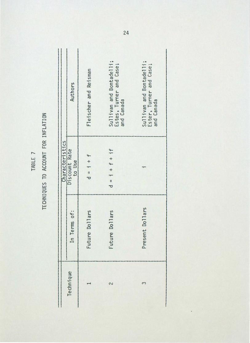
These three major inflation techniques can be summarized

in Table 7.

Am

ount

at

Per

iod

S

tart

of

Per

iod

1 p

2 P(

1+

i) (

1+f)

3 P

(1+

i)2

(1+

f)2

. .

. .

. .

TABL

E 6

TABU

LAR

BREA

KOUT

OF

COMP

ONEN

TS O

F TE

CHNI

QUE

#2

Inte

rest

In

flati

on

I n

f 1 at i

on

on

Am

ount

at

End

Dur

ing

Dur

ing

Inte

rest

o

f P

erio

d

Per

iod

P

erio

d

Ret

urn

i . p

f·

P

f·iP

P

+iP

+fP

+f(

iP)=

P(1

+i)

(1+

f)

; . p

( 1 +

i) (

1 +f)

f·

P(1

+i)

(1+

f)

f. i

p ( 1

+i )

( 1 +

f)

P(1

+i)

2 (1+

f)

i . p

( 1 +

i) 2

( 1 +

f) 2

f·P

(1+

i)2

(1+

f)2

f.;

p ( 1

+i )

2 ( 1

+f)

2 P

(1+

i)3

(1+

f)

. .

. .

. .

. .

. .

. .

2 3

N w

Tec

hniq

ue

1 2 3

--

·--~

TABL

E 7

TECH

NIQU

ES

TO A

CCOU

NT

FOR

INFL

ATIO

N

Cha

ract

eris

tics

In

Ter

ms

of:

Dis

coun

t R

ate

Aut

hors

to

Use

Futu

re

Do 11

ars

d

=

i +

f

Fle

isch

er a

nd

Rei

sman

Futu

re D

o 11 a

rs

d =

i

+ f

+ if

S

ulli

van

and

Bon

tade

lli;

E

stes

, T

urne

r an

d C

ase;

an

d C

anad

a

Pre

sent

Do 1

1 ars

i

Sul

liva

n an

d B

onta

dell

i;

Est

er,

Tur

ner

and

Cas

e;

and

Can

ada

'----

----

---

--~

--

-------

---

N +::>

-

CHAPTER V

COMPARISON OF INFLATION TECHNIQUES

Comparison of Techniques

A survey of engineering economy literature produces three ma­

jor techniques to account for inflation. For comparison purpose,

assume that the present worth formula is used, and these three tech­

niques can be illustrated as:

1. Letting R0 be the amount of money in present dollars

for period ·zero and ft"j be the amount of money in future do 11 ars

for period j, the first technique, which deals with future dol­

lars, computes the present worth equivalent of a series of flj

by the equation:

n PW = I A.(1 + i + f)-j

j=O J

n . or PW = I A.(1 + d)-J where d = i + j

j=O J

( 8)

(9)

2. The second technique, also dealing with future dollars,

has the equation:

n . . PW = I A.(1 + i)-J(l + f)-J

j=O J

or PW n

= I A.(1 + i + f + if)-j j=O J

25

(10)

( 11)

26

n or PW = ~ A-(1 + d)-j where d = i + f + if (12)

j=O J

3. The third technique, which is based on present dol­

lars, calculates the present worth equivalent of a series of R 0

as:

n . PW = ~ R (1 + i)-J

j=O o

In order to determine if a technique is appropriate

(13)

to account for inflation, each must be analyzed and evaluated in

terms of advantages and disadvantages in relation to investment

projects. This can be accomplished by applying these three tech­

niques to an example problem.

Example 3

An investment of $5,000 for a new machine is being con-

sidered. The new machine will save, in present or constant dol­

lars, $2,000 per year for the next three years, at which time

it will possess, after its removal, zero salvage value. If

the rate of return is 10% and the estimated inflation rate of

the general economy during the analysis period is 8%, should

the investment be selected?

Solution of Technique #1: See Table 8

1. The $2,000 savings are converted from present dol-

lars to future dollars year by year, using equation (6) witb f=8%.

27

2. Discount the $2,000 savings in future dollars to the

present worth of each year by the combined discount rate: d=i+f.

3. The present worth of the investment, which is the sum

of all discounted values calculated in #2 above, is $39.29. Thus,

the investment should be selected.

TABLE 8

COMPUTATION OF PRESENT WORTH USING TECHNIQUE #1

Period Cash Flow in Cash Flow in Present Worth Present Do 11 ars Future Do 11 ars @ d = ; + f

0 $ -5,000 $-5,000. $-5,000.

1 2,000 2,160.00 1,830.51

2 2,000 2,332.80 1,675.38

3 2,000 2,519.42 1,533.40

$ 39.29

Solution of Technique #2: See Table 9

1. The $2,000 savings, which are given in present dollars,

are inflated to future dollars by equation (6) with f = 8%.

2. They are discounted next to the present worth of each

year by the combined discount rate: d = i + f + if.

3. The present worth of the investment is $-26.30, showing

that the investment is not attractive.

28

TABLE 9

COMPUTATION OF PRESENT WORTH USING TECHNIQUE #2

Period Cash Flow in Cash Flow in Present Worth Present Dollars Future Dollars @ d = i+f+i f

0 $- 5,000 $~5,000. $-5,000.

1 2,000 2,160.00 1,818.18

2 2,000 2,332.80 1,652.89

3 2,000 2,519.42 1,502.63

$- 26.30

Solution of Technique #3: See Table 10

1. The $2,000 savings are already estimated in present

dollars; they do not need to be changed.

2. Discount them to present worth using the rate of

return, i.

3. The present worth of the investment is $-26.30, 1n­

~icating an unfavGrable investment.

The results obtained from three inflation techniques

can be summarized in Table 11. It is noted that the second and

third techniques have the same present value (~$26.30). This is to

be expected, even though these two techniques are solved under

different procedures. The third technique measures the $2,000

savings of each year in the constant dollars used in year zero

and then discounts them to present worth values using a discount

Period

0

1

2

3

Technique

1

2

3

29

TABLE 10

COMPUTATION OF PRESENT WORTH USING TECHNIQUE #3

Cash Flow in Present Worth Present Do 11 ars @ d = i

$- 5,000 $-5,000.

2,000 1,818._8

2,000 1,652.89

2,000 1,502.63

$- 26.30

TABLE 11

COMPARISON OF RESULTS OBTAINED FROM THREE INFLATION TECHNIQUES

Cash Flows in: Discount Present Worth Rate Used

Future Dollars d=i+f $ 39.29

Future Dollars d=i+f+i f $-26.30

Present Dollars d = i $-26.30

30

rate which takes out only the increase due to the earning power,

i . e . , rate of re turn :

( 14)

The second technique, in contrast, estimates the $2,000

savings of each year in the inflated dollars current in the year

they are occurring and then converts them to their equivalent

present values with a combined discount rate which considers

both the earning power and the inflation aspect:

R ( 1 + f)j PW =

0 .

(1 + d)J where d = i + f + if

R ( 1 + f)j or PW = --0--=---~

(1 + i)j(l + f)j

canceling out the factor (1 + f)j:

Ro PW = ----..-

(1 + i)J

( 15)

( 16)

(17)

which is equivalent to equation 14. This implies how the second

technique maintains the equivalency concept when introducing in­

flation into computations.

If the inflated dollars are discounted using only the rate

of return (see Table 12):

R ( 1 + f) j 0

PW = ------(1 + i)j

(18)

the present worth obtained now becomes more attractive ($784.45).

However, this approach is incorrect. The present worth values of

31

savings are all overstated. For example, at period t = 1, the

$2,160 is interpreted to be the amount of dollars necessary to

have the same purchasing power as $2,000 in year zero. The $2,160

- $2,000 = $160 increment is a measure of what the savings at that

point in time must be needed to be equivalent to this $2,000, but

not an increase in value. Taking out the $160 increment needed

for inflation brings back to $2,000, which, when discounted at 10%,

becomes $2,000 (1 + 0.1)-1 = $1,818.18. Thus, the overstatement

of $1,963.64 - $1,818.18 = $145.46 can be explained as the present

value of the needed $160, since $160 (1 + 0.1)-1 = $145.46. A

similar argument holds for periods two and three.

Period

0

1

2

3

TABLE 12

COMPUTATION OF PRESENT WORTH USING TECHNIQUE #2 BUT AT A DISCOUNT RATE, i

Cash Flow in Cash Flow in Present Worth Present Do 11 ars Future Do 11 ars @ ; = 10%

$- 5,000 $- 5,000.00

2,000 $ 2,160.00 1,963.64

2,000 2,332.80 1,927.93

2,000 2,519.42 1,892.88 $ 784.45

If inflated dollars are converted to their equivalent present

worth values with a discount rate as the first technique employs: R (1 + f)j

PW = o where d = i + f (1 + d)j

32

Again, the present · worth is overstated ($39.28). This approach

inflates the savings appropriately but does not insure the dis­

count rate on element to deflate them correctly. Its discount

rate is missing the product term (i.f). Consequently, the savings

expressed in inflated dollars are discounted with a lower discount

rate. For example, consider Tables 8 and 9, at period t = 1,

the overstatement $1830.51 - $1818.18 = $12.33 is resulted when

discounting the $ 160 savings with the discount rate d where

d = i + f.

To this point, the comparison has been made based on the equi­

valency concept when introducing inflation into computations.

Now, in view of individual concepts, it is observed that the first

and second techniques ~ook at inflation differently. The first

technique considers inflation and the cost of money separately,

the second technique does not. This difference can be explained

why the present worth calculated by the first technique ($39.29)

is higher than the present value computed by the second technique

($26.30). The product term (i.f) must be taken into account

since it represents the general inflation on the real return (or

price adjustment) increment which adds the amount needed to ad­

just the real return (or price adjustment) from future dollars

with reference year (j-1) to future dollars in year j (see Tables

8 and 9).

In summary, it appears that the second and third techniques

validly account for inflationary effects. There are two r~asons:

33

1. They maintain the equivalency concept.

2. They distinguish correctly the earning power and purchasing power of money.

In fl ati on Mode 1 s

Until now, it has been assumed that all affected cash flows

escalate uniformly at the inflation rate of the general economY.

In other words, for each cash flow of element k, the price esca­

lation rate, ek, is equal to .the general inflation rate, f. It

is not a realistic assumption of course, but it makes it easier

to examine and compare different inflation techniques.

In reality, during inflation, each element escalates differ­

ently; its escalation rate may be above, equal or below the gen­

eral inflation rate. Furthermore, it may vary over time. Dif­

ferent models can be developed to reflect these possibilities.

Reconsider the base case where a uniform general inflation

rate applies equally to all elements.

Case of a Uniform General Inflation Rate Applying Equally to All Elements

Let f be the inflation rate, Rko be the cash ' flow in present

dollars of element k for period zero and Akj be the cash flow

in future dollars of element k for period j.

Using the present dollar analysis technique, the present

worth equivalent is computed as follows:

34

m n PW = r r Rko (1 + i)-j

k=O j=O

The future dollar analysis technique computes the present

worth as fo 11 ows:

m n PW = r r AkJ. (1 + i)-j (1 + f)-j

k=O j=O

where: Akj = Rko (1 + f)j

Case of Different but Uniform Price Escalation Rates and a Uniform General Inflation Rate

Now, th.e two basic roodels can be revised to reflect the

( 12)

( 13)

( 14)

possibility that not all elements will be affected by the general

inflation rate, i.e., energy costs may be escalated uniformly at

the rate of 15%, material costs at 12% and so forth, but the gen­

eral inflation rate is 8%.

Assume ek and e'k as the price escalation rates and differ­

ential price escalation rate of element k, the basic model of the

present dollar analysis technique will be changed to:

m n PW = E E [Rko (1 + e'k)jl (1 + i)-j

k=O j=O

where: e - f k e' = ---k 1 + f

since these elements escalating at a rate greater (or smaller)

than the general inflation rate must be enlarged (deflated) at

( 15)

(16)

35

a rate e'k. The relationship between the general inflation rate,

f; price escalation rate, ek; and differential price escalation,

e'k is defined as:

(17)

or

ek = f + e' k + f · ek ( 18)

The following example is used for illustrating the equation above:

Example 3

The annual ene_rgy cost estimate is $2,000 in year zero with

projected escalation of 15% per year and a general inflation of

6%. The computations are shown in Table 13.

For the future dollar analysis technique, the present worth

will be:

m n PW = L r AkJ. (1 + i)-j (1 + f)-j

k=O j=O

where: Akj = Rko (1 + ek)j

Case of Period-by-Period Variations in Different Price Escalation Rates and in the General Inflation Rate

( 19)

(20)

Now, assuming that the general inflation rate and price es­

calation rates tend to change from one time period to the next,

the new model for the present dollar analysis technique will be:

36

where: ek. - f. e • - J J

kj - 1 + f. J

(22)

and for the future dollar analysis technique:

m n n PW = L L Ak. TI (1 + i)-j (1 + f.)-j (23)

k=O j=O J j=O J

Estimated Annual

Period Cost at Beginning of Year

1 $2,000

2 2,300

3 2,645

TABLE 13

TABULAR BREAK OUT OF COMPONENTS IN ANNUAL PRICE ESCALATION RATE

Annua 1 Cost General Cost Change Change Inflation

Due to Increment on Price Price Due to Adjustment Price Adjustment Adjustment I ncrerren t

$120 $170 $10

138 195 12

159 225 13

Numerical Example

(24)

Estimated Annual Cost at

End of Year

$2,300

2,645

3,042

To further demonstrate the two inflation techniques which

are accepted as va 1 i d and to i 11 ustrate correct procedures to

use when performing engineering economY studies, the following

example is presented:

37

Example 4

A firm is considering the pros pect of replacing a current

manual handling operation with a new powered conveyor system.

The cost and financial data are assumed as:

1. Installed cost for the new system is $120,000 with an estimated salvage value of $20,000 at the end of a ten-year period.

2. Labor savings are estimated to be $60,000 per year; energy costs, $15,000 per year; maintenance costs, $12,000 per year; and parts for replacement, $8,000 per year.

3. The investment can be financed with either 100% equity or a mixture of 50% equity and 50% debt financing, available at 12% interest and repay­rrent to be uniform.

4. Or, the firm may lease the system. The proposed ten-year lease contract calls for an initial deposit of $24,000 which will be returned at the end of the period of the lease and a rental payment of $20,000 at the beginning of each year.

5. The firm's minimum required rate of return is 15% after taxes .

6. Sum-of-the-years-digit depreciation method is applied with the income tax rate of 50%.

7. The general economy inflation rate is expected to be 8% per year; labor and maintenance costs , 10%; energy costs, 15%; and parts for replace­ment, 8% .

Should the new powered conveyor system be installed? If installed,

should the new system be purchased or leased?

The a 1 ternati ves are first compared neglecting inflation.

As such, conventional after-tax cash flow procedures are used

here.

38

Buy With No Finance

The necessary computattons are i 11 ustrated in Table 14.

The net present value is found to be -$22, 132~40 .

Buy With 50% Debt Financing

Initial computations are computed first:

1. 50% debt financing= $120,000 x 0.5 = $60,000

2. Payment size= $60,000 (A/P, 12, 10) = $10,619.05 per year

3. Principle and interest breakout:

Payment

1

2

3

4

5

6

7 °

8

9

10

Principal

$10,619.05 (P/F, 12, 10) = $3,419.05

10,619.05 (P/F, 12, 9) = 3,829.33

10,619:05 (P/F, 12, 8) = 4,288.85

10,619.05 (P/F, 12, 7) = 4,803.51

10,619.05 (P/F, 12, 6) = 5,379.94

10,619.05 (P/F, 12, 5) = 6,025.53

10,619.05 (P/F, 12, 4) = 6,748.59

10,619.05 (P/F, 12, 3) = 7,558.43

10,619.05 (P/F, 12, 2) = 8,465.44

10,619.05 (P/F, 12, 1) = 9,481.29

Interest

$7,200.00

6,789.72

6,330.20

5,815.54

5,239.11

4,593.52

3,870.46

3.060.62

2,153.61

1,137.76

The computations of the present worth are done in Table 15 with

the same procedure as above. Notice that only the interes t on

debt financing can be deducted for income tax, but not the prin ­

cipal. The net present worth is -$2,016.12.

Fir

st C

ost

Per

iod

and

Sal

vage

V

alue

0 $-

120,

000

1 2 3 4 5 6 7 8 9 10

10

20,0

00

TABL

E 14

COM

PUTA

TION

OF

PRES

ENT

WOR

TH

OF B

UY

ALTE

RNAT

IVE

-NO

IN

FLA

TIO

N

Mai

n-L

abor

E

nerg

y te

nanc

e P

arts

De

pre

c i a

t ion

T

axab

le

Tax

Sav

ings

C

osts

C

osts

C

osts

In

com

e

$50,

000

$-!"5

,000

$.1

2,00

0 $-

8,00

0 $-

18,1

81.8

1 $

6,81

8.18

$-

3,40

9.09

50,0

00

-15,

000

-12,

000

-8,0

00

-16,

363.

63

8,63

6.36

-

4,31

8.18

50,0

00

-15,

000

""'1

2,00

0 -8

,000

-1

4,54

5.45

10

,454

.55

-5,

227.

27

50,0

00

-15,

000

-12,

000

-8,0

00

-12,

727.

27

12,2

72.7

3 -

6,13

6.36

50,0

00

-15,

000

-12,

000

-8,0

00

-10,

909.

09

14,0

90.9

1 -

7,04

5.45

50,0

00 -

15,0

00 -

12,0

00

-8,0

00

-9,

090.

90

15,9

09.1

0 -

7,95

4.55

50,0

00

-15,

000

-12,

000

-8,0

00

-7,

272.

73

17,7

27.2

7 -

8.86

3.63

50,0

00 -

15,0

00 -

12

,000

-8

,000

-

5,45

4.54

19

,545

.46

-9,

772.

73

50,0

00 -

15,0

00 -

12,0

00 -

8,00

0 -

3,63

6.36

21

,363

.64

-10,

681.

82

50,0

00 -

15

' 000

-1

2,00

0 -8

,000

-

1,81

8.18

23

,181

.82

-11,

590.

91

NPV

(15

%) =

$-2

2,13

2.40

ATCF

$-12

0,00

0.00

21,5

90.9

1

20,6

18.8

2

19.7

72.7

3

18,8

63.6

4

17,9

54.5

5

17.0

45.4

5

16.1

36.3

7

15.2

27.2

7

14.3

18.1

8

13,4

09.0

9

20,0

00.0

0

w

c..o

Fir

st C

ost

Per

iod

and

Sal

vage

V

alue

0 $-

60,0

00

1 2 3 4 5 6 7 8 9 10

10

20,0

00

TABL

E 15

COM

PUTA

TION

OF

PRES

ENT

WORT

H OF

BUY

ALT

ERNA

TIVE

-50

% D

EBT

FINA

NCIN

G -

NO I

NFLA

TION

Mai

n-Lo

an

Loan

L

abor

E

nerg

y te

nanc

e P

arts

D

epre

ciat

ion

Tax

able

P

rin

cip

le

Inte

re·s

t S

avin

gs

Cos

ts

Cos

ts

Cos

ts

Inco

me

$-3,

419.

05

$-7,

200.

00

$60,

000

$-15

,000

$-

12,0

00

$-8,

000

$-18

,181

.81

$-38

1.82

-3,8

29.3

3 -6

,789

.72

60,0

00

-15,

000

-12,

000

-8,0

00

-16,

363.

63

1,84

6.65

-4,2

88.8

5 -6

,330

.20

60,0

00

-15,

000

-12,

000

-8,0

00

-14,

545.

45

4,12

4.35

-4,8

03.5

1 -5

,815

.54

60,0

00

-15,

000

-12,

000

-8,0

00

-12,

727.

27

6,45

7.20

-5,3

79.9

4 -5

,239

.11

60,0

00

-15,

000

-12,

000

-8,0

00

-10,

909.

09

8,85

1. 8

0

-6,0

25.5

3 -4

,593

.52

60,0

00

-15,

000

-12,

000

-8,0

00

-9,

090.

90

11 ,3

15. 6

0

-6,7

48.5

9 -3

,870

.46

60,0

00

-15,

000

-12,

000

-8,0

00

-7

,272

. 73

13,8

56.8

0

-7,5

58.4

3 -3

,060

.62

60,0

00

-15,

000

-12,

000

-8,0

00

-5,

454.

54

16,4

84.8

0

-8,4

65.4

4 -2

,153

.61

60,0

00

-15,

000

-12,

000

-8,0

00

-3,

636.

36

19,2

10.0

0

-9,4

81.2

9 -1

,137

.76

60,0

00

-15,

000

-12,

000

-8,0

00

-1,

818.

18

22,0

44.1

0

NPV

(15%

) =

$-2

,016

.42

Tax

$ 19

0.91

-92

3.32

-2,

062.

17

-3,

228.

60

-4,

425.

90

-5,

657.

80

-6,

928.

40

-8,

242.

40

-9,

605.

00

-11,

022.

05

ATCF

$-60

,000

.00

14,5

71.9

0

13,4

57.6

0

12,3

18.8

0

11,1

52.3

0

9,95

5.04

8,72

3.15

7,45

2.53

6.13

8.52

4,77

5.53

3,35

8.92

20,0

00.0

0

~

0

41

Lease

It is noted that because each year ' s rental is prepaid,

the effect on taxable income applies to the year following the

payment date; the influence on cash flow for income taxes of each

item of cash flow for rental occurs one year after the rental

payment. Of course, the $24,000 negative cash flow for the de­

posit at year zero and the $24,000 positive cash flow for the

refund at the end of lease have no effect on taxable income.

The computations are in Table 16 which shows a net present value

of $-27,101.04.

In summary, the results calculated from these three alter-

natives are:

A 1 ternati ve

Buy with no finance

Buy with 50% debt fi"nancing

Lease

Net Present Worth

$-22,132.40

- 2,016.12

-27,101.04

Therefore, in this case, the new powered conveyor system should

not be installed.

Now, three alternatives are examined in view of inflation.

Buy With No Finance

Both inflation techniques are used here. In the future

dollar analysis technique (see Table 17):

1. The labor savings and energy, maintenance and parts costs are escalated values by:

leas

e P

erio

d D

epos

it

0 $-

24,0

00

1 2 3 4 5 6 7 8 9 10

10

24,0

00

TABL

E 16

COM

PUTA

TION

OF

PR

ESEN

T W

ORTH

OF

LE

ASE

ALTE

RNAT

IVE

-NO

IN

FLA

TIO

N

Lea

se

Lea

se

Paym

ent

Lab

or

Ene

rgy

Mai

n-P

arts

T

axab

1 e

Paym

ent

on

Sav

ings

C

osts

te

nanc

e C

osts

In

com

e Ta

x T

axab

le

Cos

ts

Inco

me

$-22

,000

-22,

000

$-22

,000

$6

0,00

0 $-

15,0

00 $

-12,

000

$-8,

000

$3,0

00

$-1,

500

-22,

000

-22,

000

60,0

00

-15,

000

12,0

00

-8,0

00

3,00

0 -1

,500

-22,

000

-22,

000

60,0

00

-15,

000

12,0

00

-8,0

00

3,00

0 -1

,500

-2

2,00

0 -2

2,00

0 60

,000

-1

5,00

0 -1

2 ,0

00

-8,0

00

3,00

0 -1

,500

-2

2,00

0 -2

2,00

0 60

,000

-1

5,00

0 -1

2,00

0 -8

,000

3,

000

-1,5

00

-22,

000

-22,

000

60,0

00

-15,

000

-12,

000

-8,0

00

3,00

0 -1

,500

-2

2,00

0 -2

2,00

0 60

,000

-1

5,00

0 -1

2,00

0 -8

,000

3,

000

-1,5

00

-22,

000

-22,

000

60,0

00

-15,

000

-12,

000

-8,0

00

3,00

0 -1

,500

-2

2,00

0 -2

2,00

0 60

,000

-1

5,00

0 -1

2' 0

00

-8,0

00

3,00

0 -1

,500

-2

2,00

0 60

,000

-1

5,00

0 -1

2,00

0 -8

,000

3,

000

-1,5

00

NPV

(15

%)

= $

-27,

101.

04

AFTC

$-46

,000

1,50

0

1,50

0

1,50

0

1,50

0

1,50

0

1,50

0

1,50

0

1,50

0

1,50

0

23,5

00

24,0

00

+::o

N

TABL

E 17

COM

PUTA

TION

OF

PR

ESEN

T l~lORTH

OF

BUY

ALT

ERN

ATI

VE

-NO

FI

NA

NCE

-

8%

INFL

ATI

ON

U

SIN

G

THE

FUTU

RE

DOLL

AR

AN

ALY

SIS

TECH

NIQ

UE

Fir

st C

ost

Lab

or

Ene

rgy

Mai

nten

ance

P

arts

an

d T

axab

le

Per

iod

Sal

vage

Val

ue

Sav

ings

C

osts

C

osts

C

osts

D

epre

ciat

ion

In co

ne

Tax

AFTC

at

8%

at

10%

at

15%

@

10%

@

8%

0 $-

120,

000.

00

1 $6

6,00

0.00

$-

17,2

50.0

0 $-

13,2

00.0

0 $-

8,64

0.00

$-

18,1

81.8

1 $

8,72

8.18

$-

4,36

4.0

9 $2

2,54

5.91

2 72

,600

.00

-19,

837.

50

-14,

520.

00

-9,

331.

20

-16,

363.

63

12,5

47.7

0 -

6,27

3.85

22

,637

.50

3 79

,860

.00

-22,

813.

12

-15,

972.

00

-10.

077.

69

-14,

545.

45

16,4

51.7

0 -

8,22

5.85

22

,771

.30

4 87

,846

.00

-26,

235.

09

-17,

564.

20

-10,

883.

91

-12,

727.

27

20,4

30.5

0 -1

0,21

5.2

5 22

,942

.50

5 96

,630

.60

-30,

170.

35

-19,

326.

12

-11,

754.

62

-10,

909.

09

24,4

70.4

0 -1

2,23

5.20

23

,144

.30

6 10

6,29

3.60

-3

4,69

5.91

-2

1,25

8.73

-1

2,69

4.99

-

9,09

0.90

28

,553

.10

-14,

276.

55

23,3

67.5

0

7 11

6,92

3.03

-3

9,90

0.29

-2

3,38

4.60

-1

3,71

0.59

-

7,27

2.03

32

,654

.80

-16,

327

.40

23,6

00.1

0

8 12

8.,6

15.3

3 -4

5,88

5.34

-2

5,72

3.06

-1

4,80

7.44

-

5,45

4.54

36

.744

.90

-18.

372.

45

23,8

27.0

0

9 14

1,47

6.86

-5

2,76

8.14

-2

8,29

5.37

-1

5,99

2.03

-

3,63

6.36

40

'785

. 00

-20,

392.

50

24,0

28.8

0

10

155,

624.

55

-60,

683.

36

-31,

124.

91

-17,

271.

40

-1,

818.

18

44,7

26.7

0 -2

2,36

3.35

24

,181

.50

10

43,1

78.5

0 f

43,1

78.5

0 ---

·--

·---

·-L

_

----

·-

'---

----

· ---

·-

NPV

(at

24.2

%)

= $

-30,

932.

60

~

w

44

2. Depreciation, which is accounted for in the year indicated and occurs in future dollars, remains unchanged ~

3. The combined discount rate is employed:

d = i + f + if

4. The net present value is found to be $-30,932.60.

By the present dollar analysis technique (see Table 18):

1. It is noted that the price escalation rates of labor savings, energy and maintenance costs exceed the general inflation rqte. They must be enlarged by the factor (1 + e'k)J where: _ f

e• = ek k 1 + f

when converting them to present dollar values.

2. Depreciation, which is given in future dollars, must be changed to present dollars by the infla­tion factor.

3. The rate of return, i, is used.

4. The net present worth is $-30,932.20.

Buy With 50% Debt Financing

Using the future dollar analysis technique (see Table 19):

1. Again, all cash flows but loan principal and loan interest are projected from present dol­lars to future dollars.

2. Only the loan interest can be deducted for in­come tax but not the loan principal.

3. The combined rate is used when discounting after tax cash flows to present worth values.

4. The net present value is found to be $609.60 .

Peri

od

0 1 2 3 4 5 6 7 8 9 10

10

TABL

E 18

COM

PUTA

TION

OF

PRES

ENT

WORT

H OF

BUY

ALT

ERNA

TIVE

-

NO F

INAN

CE -

8% I

NFLA

TION

US

ING

THE

PRES

ENT

DOLL

AR A

NALY

SIS

TECH

NIQU

E

. '

Fir

st C

ost

Labo

r En

ergy

M

aint

enan

ce

Par

ts

Dep

reci

atio

n T

axab

le

and

Savi

ngs

Cos

ts

Cos

ts

Tax

Salv

age

Val

ue

at 1

.85%

at

6.4

8%

at 1

.85%

C

osts

at

7.4

1%

Inco

me

$-12

0,00

0.00

$61

'110

.00

$-15

,972

.00

$-12

,222

.00

$-8,

000

$-16

,834

.53

$ 8,

081.

47

$-4,

040.

73

62,2

40.5

3 -1

7,00

6.98

-1

2,44

8.10

-8

,000

-1

4,02

8.39

10

,757

.06

-5,

378.

53

63,3

91.9

8 -1

8,10

9.03

-1

2,67

8.39

-8

,000

-1

1,54

5.67

13

,058

.89

-6.

529.

44

64,5

64,7

3 -1

9,28

2.50

-1

2,91

2.94

-8

,000

..

9,35

3.87

15

,015

.42

.. 7,

507

.71

65,7

59.1

8 -2

0,53

2.01

-1

3,15

1.83

-8

,000

-

7,42

3.50

16

,651

.84

-8,

325.

92

66,9

75.7

2 -2

1,86

2.48

-1

3,39

5.14

-8

,000

-

5,72

7.84

17

,990

.26

-8.

995.

13

68,2

14.7

8 -2

3,27

9.17

-1

3,64

2.95

-8

,000

-

4,24

2.73

19

,049

.93

.. 9,

524.

96

69,4

76.7

5 -2

4,78

7.66

-1

3,89

5.35

-8

,000

-

2,94

6.25

19

,847

.49

-9,

923.

74

70,7

62.0

7 -2

6,39

3.90

-1

4,15

2.41

-8

,000

-1

,01

8.6

2

20.3

97.1

4 -1

0,19

8.57

72,0

71 .1

7 -2

8,10

4.23

-1

4,41

4.23

-8

,000

-

841.

93

20,7

10.7

8 -1

0,35

5.39

20,0

00.0

0

NPV

(at

15%

) =

$-30

,93

2.20

..

T

..

-.

T

AFTC

$120

,000

.00

20,8

7 .. 5.

27

l9,3

96.9

2

18.0

75.1

2

16,8

61.6

0

15,7

49.4

2

14,7

23.0

0

13,7

67.7

0

12,8

70.0

0

12.0

17.2

0

11 ,

197.

32

20,0

00.0

0

+==a

U

1

Per

iod

0 1 2 3 4 5 6 7 8 9 10

10

TABL

E 19

COM

PUTA

TION

OF

PRES

ENT

WORT

H OF

BUY

ALT

ERNA

TIVE

-50

%

FINA

NCIN

G -

8%

INFL

ATIO

N US

ING

THE

FUTU

RE

DOLL

AR A

NALY

SIS

TECH

NIQU

E

Fir

st C

ost

Lab

or

Ene

rgy

Mai

nten

ance

P

arts

an

d Lo

an

Loan

T

axab

le

Sal

vage

P

rin

cip

al

Inte

rest

S

avin

gs

Cos

ts

Cos

ts

Cos

ts

Dep

reci

atio

n In

com

e Ta

x

Val

ue

@ 8%

@

10

%

@ 15

%

@ 10

%

@ 8%

$-60

,000

.00

$-3,

419.

05

$-7,

200.

00

$ 66

,000

.00

$-17

,250

.00

$-13

,200

.00

$-8,

640.

00

$-18

,181

.81

$ 1,

528.

18

$-76

4.09

-3,8

29.3

3 -6

,789

.72

72,6

00.0

0 -1

9,83

7.50

-1

4,52

0.00

-

9 ,3

31. 2

0 -1

6,36

3.63

5,

757.

94

-2,

878.

97

-4,2

88.8

5 -6

,330

.20

79,8

60.0

0 -2

2,81

3.12

-1

5,97

2.00

-1

0,07

7.69

-1

4,54

5.45

10

,121

.50

-5,

060.

75

-4,8

03.5

1 -5

,815

.54

87,8

46.0

0 -2

6,23

5.09

-1

7,56

9.20

-1

0.88

3.91

-1

2,72

7.27

14

,615

.00

-7,

307.

50

-5,3

79.9

4 -5

,239

.11

96,6

30.6

0 -3

0,17

0.35

-1

9,32

6.12

-1

1,75

4.62

-1

0,90

9.09

19

,231

.30

-9,

615.

65

-6,0

25.5

3 -4

,593

.52

106,

293.

66

-34,

695.

91

-21,

258.

73

-12,

694.

99

-9,

090,

90

23.9

59.0

0 -1

1,97

9.80

-6,7

48.5

9 -3

,870

.46

116,

923.

03

-39,

900.

29

-23,

384.

60

-13,

710.

59

-7,

272.

73

28,7

84.4

0 -1

4,39

2.20

-7,5

58.4

3 -3

,000

.62

128,

615.

33

-45,

885.

34

-25.

723.

06

-14,

807.

44

-5,

454.

54

33,6

84.4

0 -1

6,84

2.15

-8,4

65.4

4 -2

,513

.61

14h4

76. 8

6 -5

2.76

8.14

-2

8,29

5.37

-1

5,99

2.03

-

3,63

6.36

38

,631

.30

-19,

351.

65

-9,4

81.2

9 -1

,137

.76

155,

624.

55

-60,

683.

36

-31,

124.

91

-17,

271.

40

-1,

818.

18

43,5

88.9

4 -2

1,79

4.47

43,1

78.5

0 -

--

---

---

-----

--

NPV

(24.

2%}

= $

609.

60

AFTC

$15,

526

.90

15,4

13.3

0

15,3

17.4

0

15.2

31.2

0

15,1

44.8

0

15.0

45.2

0

14,9

16.3

0

14,7

39.3

0

14,4

86.6

0

14 t 1

31.3

6

43,1

78.5

0

~

0"1

47

Lease

By the future dollar analysis technique (see Table 20):

1. As previously, all cash flows, which include ~osts, savings but not least deposit or payments, are escalated.

2. The combined discount rate is used.

3. The net present worth is $-4,134.70.

In sum~ary, the results show:

Alternative

Buy with no finance (using the future dollar analysis technique)

Buy with no finance (using the real dollar analysis technique)

Buy with 50% debt financing

Lease

Net Present Worth

$-30,932.60

-30,932.40

609.60

- 4,134.70

Thus, in view of 8% inflation of the general economy, the new

powered conveyor system should be bought with 50% debt financing.

It is noted that, when inflation is present, purchasing

becomes more co~tly but purchasing with 50% debt financing and

leasing become· less costly. This is because loan and lease

payments are not responsive to inflation and have tax advantages .

It is also noted that the future and present dollar analysis ·

techniques provide the same results.

Pe

rio

d

Leas

e D

ep

osit

0 $-

24,0

00

1 2 3 4 5 6 7 8 9 10

10

24,0

00

TABL

E 20

COM

PUTA

TION

OF

PRES

ENT

WORT

H OF

LEA

SE A

LTER

NATI

VE -

8%

INFL

ATIO

N -

USIN

G TH

E FU

TURE

DO

LLAR

ANA

LYSI

S TE

CHNI

QUE

Leas

e L

ab

or

En

erg

y M

ain

ten

an

ce

Pa

rts

Leas

e P

aym

ent

Sa

vin

gs

Co

sts

Co

sts

Co

sts

Ta

xab

le

Tax

ATC

F P

ayr

ren

t on

@

10%

@

15%

@

10%

@

8%

Inco

me

Ta

xab

le

Inco

me

$-22

,000

$-

46,0

00.0

0

-22.

,000

$-

22,0

00

$ 66

,000

.00

$-17

,250

.00

$-13

,200

.00

$-8,

640.

00

$ 4,

910.

00

$-2,

455.

00

2,45

5.00

-22,

000

-22,

000

72,6

00.0

0 -1

9,83

7.50

-1

4,52

0.00

-

9,33

1.20

6,

911.

29

-3,

455.

64

3,45

5.64

-22,

000

-22,

000

79,8

60.0

0 -2

2 ,8

13.1

2 -1

5,97

2.00

-1

0,07

7.69

8,

997.

18

-4,

498.

59

4,49

8.59

-22,

000

-22,

000

87,8

46.0

0 -2

6,23

5.09

-1

7,56

9.20

-1

0,88

3,91

11

,157

,80

-5,

578.

90

5,57

8.90

-22,

000

-22,

000

96,6

30.6

0 -3

0,17

0.35

-1

9,32

6.12

-1

1,75

4.62

13

,379

.50

-6,

689.

75

6,68

9.75

-22,

000

-22,

000

106,

293.

60

-34,

695.

91

-21,

258.

73

-12,

694.

99

15,6

44.0

0 -

7,82

2.00

7,

822.

00

-22,

000

-22,

000

116,

923.

03

-39,

900.

29

-23,

384.

60

-13,

710.

59

17,9

27.5

0 -

8,96

3.75

8,

963.

75

-22,

000

-22,

000

128,

615.

33

-45,

885.

34

-25,

723.

06

-14,

907.

44

20,1

99.5

0 -1

0,09

9.75

10

,099

.75

-22,

000

-22,

000

141,

476.

86

-52,

768.

14

-28,

295.

37

-15,

992.

03

22,4

21.3

0 -1

1,21

0.65

11

,210

.65

-22,

000

155,

624.

55

-60,

683.

36

-31,

124.

91

-17,

271.

40

24,5

44.9

0 -1

2,27

2.45

34

.272

.45

24,0

00.0

0 >

----

----

---

-

NPV

(@

24.2

%)

= $

-4,1

34.7

0

..,J:=

. 0

0

CHAPTER VI

CONCLUSIONS AND RE COM~1ENDATI ONS

Co n c l us i on s

This paper has concentrated on the study of major inflation

techniques used in engineering economy studies. Three such tech­

niques were discussed and evaluated, using the present worth

analysis as a basis. The following conclusions are observed:

1. The first technique is not valid. It did not recognize

the general inflation on the real return increment or the price

adjustment increment, which adds the amount needed to adjust the

real return increment or the price adjustment increment from

future dollars with reference year (j-1) to future dollars in

year j. This error makes investment projects appear more desir­

able than they actually are, when using the discount rate (d=i+f).

2. The second and third techniques are found to be valid

to account for inflation. They distinguished correctly between

the earning power and the purchasing power, and maintained

the equivalency concept when introducing the effects of inflation

into computations.

3. The second technique estimates future cash flows in

future dollars appropriately, using the projected

49

50

escalation rates. The third technique requires that future cash

flows be made relative to equivalent purchasing power in year

zero. This is not as easy as it would first appear. Lease .

and loan payments, which are contractually measured in future

dollars, must be de-escalated to present dollar values in year zero.

Also, when costs are increasing or dec~easing in price differ-

ently, these differences must be estimated just as the total in-

crease or decrease in price for each cost is projected in the

future dollar analysis technique.

Recommendations

In view of the findings of this paper, the following recom-

mendations are made:

1. The second technique, known as the future dollar analysis

technique, is the most appropriate to use when accounting for in-

flation.

2. A recommended procedure is as follows:

a. Express all cash flow components each period in future dollars current in the period they occur­red.

b. Compute after-tax cash flow values for each period.

c. Calculate present worth values of after-tax cash flow values for each period, using the combined discount rate (d = i + f +if).

3. Faced with the difficulty of projecting the magnitude of

future inflation, it is suggested a sensitivity analysis be per-

formed over a range of i nfl ati on rates.

51

4. For the purposes above, a computer program written in

BASIC is presented. The program listing is illustrated in

Appendix A. It is completely self-documenting so the user can

enter input data as required. The outputs will be set up in

the tabularized table form, which shows present values of all

cash flows spent or received during each period and the present

worth of the investment. The program inputs and outputs of the

program are shown in Appendices B and C.

APPENDICES

APPENDIX A

PROGRAM LISTING

1 CLS 2 F..:Er'; >t.:* ECON:niC ANALYSIS F'R~GRAr. 3 REM *~ FI~C THE F'R~SENl VA~UE It E::r: X:l U~~~f:f< CDN0ITICi~ S C F I~F- LA 71QN 5 FOR I!=i TC lCCO 6 NEXT II 7 DIM N{20) B FCJF~ X=i TC 2 C 9 GJSLL 13EC 1 0 It-ci='UT N ~X) 2C IF N(i)=1 THEN 60 3: IF X>=6 TH:N 70 1ft X=6 ~a GOTO 70 60 IF X=6 THEN X=X+2 7C NE:XT X 80 Fo.::~ X=i 70 20 90 PRINT x; •. •; 10( GJSJE' 132J 11( F'Rii\T N(X) 12C IF N(1)=1 THEN 160 130 IF X>=6 THE~ i7C 140 X=6 15C G·:iTO 170 160 IF X=6 THEN X=X+2 17C NEXT X 180 PR:NT 'ELEMENT TO [E C~ANGED<C TO CALSULAT!ON)•; 190 INPUT Y 20C IF Y=O TH~N 2~0 210 PRINT 'NEW VALUE •; 220 INPUT N<Y> 230 GOTO 80 2 4 0 f' R IN T T A E ( 1 ) • p E F..::: 0 D I t T A E· ( 1 0 ) I E: FTc I ; T A E ( 2.1 ) • DE F' F ~: ll ;

2 41 f' R IN T T A E= < 3 ~ ) • T X I i'i C • ; T A E: ( .q 3 i • AFT C • ; T A£:. ( ~ "1 ) • F' h 250 IF N<1>=1 THEN 3iC 26C E:F=N(7)..-N(8) 30( GOTC "t3G 310 N=O 320 N1=CN<13)/2>•<N<13)+1) 33u E:V=NC2)

53

APPENDIX A (Continued)

3~ 0 IF N <~>>D TH~~ 37 J 3 5 0 E: F = N < 2 > 36 :· GOI·o -43 0 37 C DF=N < 2.) *r~ < 4 > /1 0 G 3EQ 1=~(5)/100

39C F=(~+I)[N (13)

~CG YP=DF~<<I•F~/(F-1)) ~:.. C E:r:·=N ~ 2.) -DF ~3C AF=EF ~4C F'\) =AF

54

~ 5 1 f' F: I NT T A E ·: 5 4 ) :!. ~'f 7 ( F· '.) *- l 8 :i ) I 1 C C ~6C Y1=r~<1S) li-7( Y1=Yi+1 If 8 Q F 0 :: ·~ X= .i T 0 N ( i. 3 ) ~90 IF N(1)=1 TH~N 5~C 5CC LF'=t\(8) 51( ~2[

c=· 4 f i ..; . ..,

IF X=N~~3) TH~~ 56[ L=LF GCTJ 570 IF N(4)>0 TH~~ 6GO

55 J LF'== C 560 L=u 570 DF'=C 5£0 590 6CG

Dl=O GCTC 614 Yl=Yi-1

6~C DP=YP~(1+N(5)/10Q)[-Yi

611 DI=YF-DF' 612 LF':C 61S L=G 614 CF=NC9) 620 R=N\17) 63G GCSUE: lQEC 6JtD Fi=CF 650 CF=N(10) 66C R=N<1E) 6 7 0 G C SUE: 1 0 E C 68C F2=CF 69G CF=N(ll) 70C R=N<:!.CT· ) 7iC· GQSJE 1080 72C F3=CF 7::o cr=N(12) 74G R=i'l(2() 75C GOE·UE 1080 760 F4=CF 77 0 E.F=L+DF'+DI+F 1 +FZ+F~ +F"l

55

APPENDIX A (Continued)

78G BT=LP+CI+F1+FZ+F3+F4 790 IF NC1)=1 THE~ 82 0 snc oc=o 810 GCTO E.30 6 2 t G 0 SUE: 11 5 J 8:30 TI=E.T+CC 8~G GDS~E: 1300 B~ f: AF=E:F+TX 86C GJSUB 1320 87 u F'\/=F'V:tF W 8 E : P E: NT TAt:~ \ i ) X ; T A E· ( 1 0 ) I r·; T ( E: F * 1 C C ) / 1 0 C ; 6E1 P~I~T TAB(21)INT<D:~.i0C )/1DO;TA~ C32>1N7<Tl~~CQ)/lOC; B62 PRINT TAB(~3>INTCAFxiO Q )/10 0;TAB:5~)lN~(FW~1CC)/1C~

890 NEXT X 695 X=N<13) 900 IF N(1)=1 THEN 93C 91(} CF=-N(7) 92C GOTC 970 9::0 CF=N<::) 95C R=N(i6) 9 6 c G C S lJ B 1 0 8 C· 97C AF=CF 960 GOSL!B 1320 99 0 F'V=Pl.i +F~

lOOC PR!~T TA8<10)INT<CF*1 0~ )/lOQ;TA[(4~;INl C AF*i00) /l :J;

10C1 PRI~T TABC54)!~7(P~ ~ 1 G0) /10C 1010 PRINT TAE(5~)u _________ • 102C PRINT TASC54>INTCPV*1C0)/100 1 C 2. c;- P ;::~IN l T A E ( 1 ) • *A i\ S W [ ~ : IF IN F LA;: 0 r. IS • ; N ( 1 6 ) ; • ;; " 1030 IF NC1)=1 THE~ PR:~T TA8<13>•DEST FINAN:ING •;N ( ~);·~·

1 0 31 T $ = • E: U Y • 1032 IF N<1>=1 THE~ it~G 1033 T$=•LEAS£L 1C~C PRINT TAE(iQ)T$;• IN~ESM~~T HAS PRZSENT WORT~ Or •; 1C~1 PRINT ;INT<PV*iCQ)/100 105C INPU7 ·E~TE~ C TC CHA~GE DATA •;z 1060 IF Z<>O THEN 179[ 1C70 GGTO 8C 1080 IF R=O THE~ llLC 1090 R=R/10G 1100 GOSUE: 1130 1110 CF=CA 1120 RETURN 1130 CA=CF~<l+R)[X 11~0 RETURN 1150 IF N<6><>1 THEN 116C 1160 OC=<N<2>+N(~))/N(13) 1170 RETURN

56 APPENDIX A (Continued)

1180 IF NC6><>2 THE~ 122 0 1190 DC=<NC2)+~(3))~CCN< i 3)-N) /N 1 > 120~ N=N+1 121 0 R.ETUF~N i22C DC=8V~2/N~1S) 12 3 0 E; V::: E V-D :: 12-lfO VE=-Ev 1250 !F VB>N(~) THEN 1~90 1260 B :~=E:V+DC

l27 D DC=EV+N(3) 128C E=J=-N ( 3) 12 9 C RET !J R :,~ 13CG TX=TI*(-N(15)/10C~

131 G F:ETURr~ 132C IF N<l>=l A~[ ~(16))( THEN 135 G 1330 D=N<14)/1CO 13<qO GOTC 12t>C 1350 D=(1+N(i~)/100)~(1+N(16)/1GC)-l 1360 PW=AF~<l~D):-X 1370 RETURN 138( IF X<>l TH~~ 1~GC 139 J F'F:!:\T • PF,Gt: LE:M r·'r'F'E ( ~ =E UY; Z=LEAf;~) 14GC IF X<>2 THE~ 1~20 1410 F'RIN7 •INITIAL COST($) 1420 IF X<>3 THE~ 1~40 1430 F'F.:INT •sALVAGE VALJ;::(~)

1~40 IF X<>4 THEN 1~6D 1 ~50 FRit\ T • DEBT FINANC:IN:; < ~~ > 1460 IF X<>5 THEN 1482 1~7C PR:NT •LOA~ INTER~ET RAT~(%)

1420 IF X<>6 THEN 15CC 149 G f'RINT • DEF R=:CIATION < 1 =SL; 2=5 YD t 3=[) L·E: ) 15CG IF X<>7 THE~ 152( 1510 PRINT •LEASE DEPJS!T(~) 1520 !F X<>B THEN 1~~0 15 3 0 F' F~ I~ T • LEAS=: F' A Y MEN 7 ( ~I Y R ) 1510 IF X<>9 THZN 15tC 15 5 0 P R::: ~ T • C 0 :; T C :=~ S AV:: N:; 0 ~- E ~EM EN T 1 ( i ) 1 ~ 6 0 - F X ·· .. . C· T H ,.... . . :! c-· E ,. ""' ~ ·= .. .;· 1 · • ;:. N ...; · U 157 0 PRINT • cos-:· OF~ SAiJING OF E!...EMEi'-l7 2 { ~ )

1580 IF X<>ll THEN l~(J 159 0 PRINT • COST 0?\ SA l...Jir'!G OF E~Er<Lr·~T 3 ( ~ )

1600 IF X<>12 TH~~ 16~0 !61C PR:NT •coST OR SAVIN~ CF ELE~~~ 7 ~ ( ~) 162C IF X<>13 THEf\~ 16~: 1630 PRINT •PERIOD ANA~YSIS<YR) 1640 IF X<>l~ THEN 1660 16!j G F'F:!NT • RATE OF RET:.:RN ( ~~)

. .. t

. .. t

. .. t

. .. ,

. .. t . .. t . .. t

. .. t

. .. t

li oL , . ..

t . ... t . .. , . ...

t

APPENDIX A (Continued)

l66C IF X<>15 THE~ 1680 167C PRINT •TAX RATE(~) 1680 IF X<>16 TH~N 17[(

57

16 9 0 F' R I:\ T • GENERAL It\ FLAT I C r~ RATE < i. ) 170C IF X<>17 THEN 1720 171 b F'F::NT • ESCALATIO i··~ EATE 1720 IF ·x<>lE THE~ 17~J 173( PRINT •ESCA~ATIGN RAT r 17~ C IF X<>19 THEN 1760 1 7 5 0 F' F~: NT • Esc A L H T I 0 ;-~ F:; IT E 1760 IF X<>20 THEN :79: 177C F'RrNT 1 ESCA~A7I:N RATE 178 C F~ETU~t· ;

179[ END

OF

OF

C?

cr

ELEMC:~-i 7

EL.EMENT

ELEM~N1"

E~EME~7

1 ( i. I

2{/.)

3 'i~}

4 ( i~)

• & , • & , . ..

f

• & f

• • t

I " ,

APPENDIX B

PROGRAM INPUTS AND OUTPUTS OF TYPE 1 (BUYS)

PRGELEM TYPE<l=BUY;2=LEAS£) 1 INITIAL CDST ($) -120 (0 0 SA~VAGf VALUE($) ZOCO O DEET FINA~CING(X, 0 LOAi~ INTERE:ST RATE< i~) 0 DEPRECIATICN(1=SL;2=SYD;3=0[8) 2 COST 0~ SAVING OF ELEM~~~ 1($) 600 GO COST OR SAVIN~ OF ELEME~T Z<~> -15000 COST OR SAVI~G OF ELEMENT S($) -12000 COST OR SAVING OF ELEME~T 4<~> -80 0C PERIGD ANALYSIS<YR> 10 RATE OF RETURN(~) 15 TAX RATE(l) 50 GENERAL INFLATION RATE(%) 0 ESCALATIGN RATE OF ELEM~NT 1(/.) 0 ESCALATICN R~TE OF ELEM~~T 2(~) 0 ESCALATION RATE OF ELE:WiEi~T 3 (X) · 0

PERIOD E:FTC DEF'R: TX Ir~C AFTC f·~

-120000 -i2 C~C(J -120C J: 1 25000 -1818~.E 681E·.18 2 i:;9J.9 1677 ·1 . ; · 2 250CO -:6.6363.6 663t· . 36 20o 31.8 156:; ,3 .-'; 3 25DCO -145~~ .5 1045"1.5 177;2.7 1~ ~,.: .9

4 250(0 -1272.7.3 122:72.7 1Eo~3.i 107:3~. :;

5 25CCG -109 C<;.i l.lfC9t.9 17S:5if.~ 8~' 26. 5L 6 2500[; -9G9C.9i 1~9C9.1 17("1 5.~ 73i.1 . :.2 7 25 0 CO -7272..73 17727.3 1~136."-:· 6 06t. . ~S

8 2500[ -~li5 .. ~. 5:: 1 s·s.q:;. 5 15~27.: l..r9 / 7. E.~.

9 2~00C -3636.37 21~63.6 1431&.2 .q :;-J.lZ 10 25COC -1Ei8.19 23181.8 13409.1 :;::,~..:;.~ ;;,

20000 20~00 ~9~ ::.67 .... ---------Z21::L.4

•ANSWER: IF INFLATION IS 0 /. DEBT FI~ANCING 0 X

BUY INVESM~~T HAS PRESENT WOR7H OF -2213~.4

58

APPENDIX C

PROGRAM INPUTS AND OUTPUTS OF TYPE 2 (LEASE)

PERI eli:)

1 2 3 1 5 6 7 8 9 10

PROBLEM TYPEC1=8UY;~=LEAS~) LEASE: DEPOSIT~$) LEASE PAYMENT<,IYR) COST OR SAVI~G OF ELEMENT 1($) COST OR SAVING OF ELEMENl 2<•> COST OR SAVING DF ELEMENT 3($) COST 0~ SAVI~G OF ELEMENI ~($)

PERIOD ANA~YSIS<YR) RATE OF RETUKN(~) TAX RATE(/.) GENERAL IN~LATION RATE<~> ESCALATION RATE OF ELEMENT 1(/.) ESCALATION RATE OF ELEMENT 2(~) ESCALATIO~ RATE OF ELEM~~T 3<X> ESCALATION RATE OF ELEM~~~ ~(k)

E;?TC DEi= F"~C TX INS -~6GOC

3000 0 3COO 3GGJ c 30[[; 3(08 0 3GCO 38CO ( 30CG 30CD c 3CGC 3n r, ,.. U"-~ 0 3DGC

3QOC 0 3JC;C 308( 0 3cu: 30(;0 0 30GC' 2150 0 G 0 30GJ 24COO

•ANSWER: IF INFLATION IS 0 ~

2 -240(.0 -2.200(.

6li000 -150JG -lZOOJ -8Q(.(j

10 15 5G 0 0 0 0 0

AFTC -460(;0

1 r- .-\..).,..,;

15jC 15CG 15CS .;t:'- j J. ...J.,; w

15(( 15C:Q 15G[: 15GO 235~(

24CLD

F',...; -46 GCC

13 c 4.:: ·~ i1 3 ·'\ .2 :;. 9 ; ~ . • ~ ~

6 57 . 62 74 5 . 7t 6 L;~ • ~r r,

5 63 .S ~ <;· [

,..._ . .:;, ;;

426.~ S

55 v~ . E4 rr- ,.._ ~ . .c,.. t.J 7 ..; 4. • • .:> __ ..,.. ______

-27J. Ci . ~

LEASE INVESME~T HAS PRES~~T WORTH OF -27101.~

59

60

LIST OF REFERENCES

1. Newnan, Donald G. Engineering Economic Analysis. San Jose, CA: Engineering Press, 1977.

2. Lee, Robert R., and Grant, Eugene L. "Inflation and Highway Economy Studies. 11 In Hi hwa Research Record Number 100, pp. 20-37. Washington, D. C.: Hi g way Researc Board of the National Academy of Sciences - National Research Coun ci 1 , 1965.

3. U.S. Department of Commerce. Statistical Abstract of the United States 1963. Washington, D.C.: U.S. Government Printing Office, 1964.

4. Sullivan, William G., and Bontadelli, James A. "The Indus­trial Engineer and Inflation." Industrial Engineering 12 (March 1980): 24-33.

5. Oxenfeld, Alfred R. Economic Principles and Public Issues.

6.

New York: Holt, Rinehart and Winston, 1961.

Haberler, Goffried. ington, D. C.:

Inflation, Its Causes and Cures. Wash­American Economic Association, 1960.

7. Ghore, P.M., and Torgersen, P.E. "The Effects of Inflation on Capital Investments. 11 Industrial Engineering 15 (July-August 1964): 201-207.

8. F 1 e i s ch e r, Ge r a 1 d A. , and Re i s man , A rn o 1 d . " In vestment De­cisions Under Conditions of Inflation." The Interna­tional Journal of Production Research 6 (February 1967): 87-95.

9. Estes, Carl B.; Turner, Wayne C.; and Case, Kenneth E. "The Shrinking Value of Money and Its Effects on Economic Analysis." Industrial Engineering 12 (March 1980): 18-22.

10. Canada, John R. Intermediate Economic Analysis for Manage­ment and Engineering. Englewood Cliffs, NJ: Prentice­Hall, Inc., 1971.

61

11. Baum, Sanford. 11 Engineering Economy and the Two Rates of Return- Mixed Mode Computations.~~ AIIE Transactions 10 (March 1978): 81-88.

12. Burford, Charles L.; Landers, Thomas L.; and Dryden, Robert D. "Analysis of Inflationary Effects on Depreciable Investments . ., In AI IE Proceedings of the 25th AI IE An­nual Conference and Convention, New Orleans, May 1974, pp. 47-56. Norcross, GA: AilE, 1974.