Companion to

“An update on the Hirsch conjecture”

Edward D. Kim∗ Francisco Santos†

Abstract

This is an appendix to our paper “An update of the Hirsch Conjec-ture”, containing proofs of some of the results and comments that wereomitted in it.

1 Introduction

This is an appendix to our paper “An update of the Hirsch Conjecture” [39],containing proofs of some of the results and comments that were omitted in it.The numbering of sections and results is the same in both papers, although notall appear in this companion. The same occurs with the bibliography, whichwe repeat here completely although not all of the papers are referenced. Thenumbering of figures, however, is correlative. Figures 1 to 6 are in [39] andFigures 7 to 16 are here.

2 Bounds and algorithms

2.1 Small dimension or few facets

*Theorem 2.1 (Klee [40]). H(n, 3) = b 2n3 c − 1.

Proof. To prove the lower bound, we work in the dual setting where our polytopeP simplicial and we want to move from one facet to another along the ridgesof P . Figure 7 shows the graph of a simplicial 3-polytope with nine vertices inwhich five steps are needed to go from the interior triangle to the most externalone (the outer face in the picture, which represents a facet in the polytope).The reader can easily generalize the figure to any number of vertices divisibleby three, adding layers of three vertices that increase the diameter by two.For a number of vertices equal to one or two modulo three, simply add one ortwo vertices in the interior of the central triangle, subdividing it into three or

∗Supported in part by the Centre de Recerca Matematica, NSF grant DMS-0608785 andNSF VIGRE grants DMS-0135345 and DMS-0636297.†Supported in part by the Spanish Ministry of Science through grant MTM2008-04699-

C03-02

1

arX

iv:0

912.

4235

v2 [

mat

h.C

O]

2 F

eb 2

010

five triangles. One vertex will not increase the diameter, but two vertices willincrease it by one.

Figure 7: Construction of simplicial 3-dimensional polytopes with 3+3k verticesand diameter 2k+1. Two steps are needed to cross each layer of skinny triangles.

For the upper bound, we switch back to simple polytopes. By double-counting, two times the number of edges of a simple 3-polytope P equals threetimes its number of vertices. This, together with Euler’s formula, implies that Phas exactly 2n− 4 vertices. Let u and v be two of them. Graphs of 3-polytopesare 3-connected (see [3], or [60]), which means that there are three disjoint pathsgoing from u to v. Since the number of intermediate vertices available for thesethree paths to use is 2n−6, the shortest of them uses at most b 2n3 c−2 vertices,hence it has at most b 2n3 c − 1 edges.

It is easy to generalize the second part in the proof to arbitrary dimension,giving the following lower bound. Observe that the formula gives the exactvalue of H(n, d) for d = 2 as well.

*Proposition 2.4.

H(n, d) ≥⌊d− 1

dn

⌋− (d− 2).

Proof. The addition of layers used in the proof of 2.1 can also be described asglueing copies of an octahedron to an already constructed simplicial 3-polytope.The gluing is along a triangle, so three new vertices are obtained. Before glu-ing, a projective transformation is made to the octahedron so that the triangleglued is much bigger than the opposite one, which guarantees convexity of theconstruction.

The generalization to arbitrary dimension is done gluing a cross-polytope,the polar of a d-cube. A cross-polytope is also the common convex hull in Rd oftwo parallel (d− 1)-simplices opposite to one another. It has 2d vertices and togo from a facet to the opposite one d steps are needed. When the cross-polytopeis glued to a given polytope its diameter grows by d−1, essentially for the samereasons that will make the proof of Theorem 3.16 work.

2

2.2 General upper bounds on diameters

The proof we offer for Theorem 2.5 is casically taken from Eisenbrand, Hahnleand Rothvoss [25].

*Theorem 2.5 (Larman [45]). For every n > d ≥ 3, H(n, d) ≤ n2d−3.

Proof. The proof is by induction on d. The base case d = 3 was Theorem 2.1.Let u be an initial vertex of our polytope P , of dimension d > 3. For each

other vertex v ∈ vert(P ) we consider its distance d(u1, v), and use it to constructa sequence of facets F1, . . . , Fk of P as follows:

• Let F1 be a facet that reaches “farthest from u” among those containingu. That is, let δ1 be the maximum distance to u of a vertex sharing afacet with u, and let F1 be that facet.

• Let δ2 be the maximum distance to u of a vertex sharing a facet with somevertex at distance δ1 + 1 from u, and let F2 be that facet.

• Similarly, while there are vertices at distance δi + 1 from u, let δi+1 bethe maximum distance to u of a vertex sharing a facet with some vertexat distance δi + 1 from u, and let Fi+1 be that facet.

We now stratify the vertices of P according to the distances δ1, δ2, . . . , δk soobtained. Observe that δk is the diameter of P . By convention, we let δ0 = −1:

Vi := {v ∈ vert(P ) : d(u, v) ∈ (δi−1, δi]}.

We call a facet F of P active in Vi if it contains a vertex of Vi. The crucialproperty that our stratification has is that no facet of P is active in more thantwo Vi’s. Indeed, each facet is active only in Vi’s with consecutive values of i,but a facet intersecting Vi, Vi+1 and Vi+2 would contradict the choice of thefacet Fi+1. In particular, if ni denotes the number of facets active in Vi we have

k∑i=1

ni ≤ 2n.

Since each Fi has vertices with distances to u ranging from at least δi−1+1 toδi, we have that diam(Fi) ≥ δi−δi−1−1. Even more, let Qi, i = 1, . . . , k be thepolyhedron obtained by removing from the facet-definition of Fi the equations offacets of P that are not active in Vi (which may exist since Fi may have verticesin Vi−1). By an argument similar to the one used for the polyhedron Q of theprevious proof, Qi has still diameter at least δi − δi−1 − 1. But, by inductivehypothesis, we also have that the diameter of Qi is at most 2d−4(ni − 1), sinceit has dimension d − 1 and at most ni − 1 facets. Putting all this together weget the following bound for the diameter δk of P :

3

δk =

k∑i=1

(δi − δi−1 − 1) + (k − 1)

<

k∑i=1

2d−4(ni − 1) + k

= 2d−4∑i

ni − k(2d−4 − 1) ≤ 2d−3n.

*Theorem 2.6 (Kalai-Kleitman [36]). For every n > d, H(n, d) ≤ nlog2(d)+1.

Proof of Theorem 2.6. Let P be a d-dimensional polyhedron with n facets, andlet v and u be two vertices of P . Let kv (respectively ku) be the maximalpositive number such that the union of all vertices in all paths in G(P ) startingfrom v (respectively u) of length at most kv (respectively ku) are incident to atmost n

2 facets. Clearly, there is a facet F of P so that we can reach F by a pathof length kv + 1 from v and a path of length ku + 1 from u.

We claim that kv ≤ Hu(bn2 c, d) (and the same for ku), where Hu(n, d) de-notes the maximum diameter of all d-polyhedra with n facets. To prove this, letQ be the polyhedron defined by taking only the inequalities of P correspondingto facets that can be reached from v by a path of length at most kv. By con-struction, all vertices of P at distance at most kv from v are also vertices in Q,and vice-versa. In particular, if w is a vertex of P whose distance from v is kvthen its distance from v in Q is also kv. Since Q has at most n/2 facets, we getkv ≤ Hu(bn2 c, d).

The claim implies the following recursive formula for Hu:

Hu(n, d) ≤ 2Hu

(⌊n2

⌋, d)

+Hu(n, d− 1) + 2,

which we can rewrite as

Hu(n, d) + 1

n≤Hu

(⌊n2

⌋, d)

+ 1

n/2+Hu(n, d− 1) + 1

n.

This suggests calling h(k, d) := (H(2k, d)−1)/2k and applying the recursionwith n = 2k, to get:

h(k, d) ≤ h(k − 1, d) + h(k, d− 1).

This implies h(k, d) ≤(k+dd

), or

Hu(2k, d) ≤ 2k(k + d

d

).

From this the statement follows if we assume n ≤ 2d (that is, k ≤ d). For n ≥ 2d

we use Larman’s bound Hu(n, d) ≤ n2d ≤ n2, proved below.

4

2.4 Some polytopes from combinatorial optimization

Small integer coordinates

*Theorem 2.11 (Naddef [50]). If P is a 0-1 polytope then diam(P ) ≤ n(P )−dim(P ).

Proof. We assume that P is full-dimensional. This is no loss of generality since,if the dimension of P is strictly less than d, then P can be isomorphicallyprojected to a face of the cube [0, 1]d.

Let u and v be two vertices of P . By symmetry, we may assume thatu = (0, . . . , 0). If there is an i such that vi = 0, then u and v are both onthe face of the cube corresponding to {x ∈ Rd | xi = 0}, and the statementfollows by induction. Therefore, we assume that v = (1, . . . , 1). Now, pick anyneighboring vertex v′ of v. There is an i such that v′i = 0. Then, u and v′ arevertices of a lower-dimensional 0-1 polytope and we have used one edge to gofrom v to v′. The result follows by induction on d.

Transportation and dual transportation polytopes

We here include the precise definition of 3-way transportation polytopes, whichwe skipped in the paper:

• 3-way axial transportation polytopes. Let a = (a1, . . . , ap), b =(b1, . . . , bq), and c = (c1, . . . , cr) be three vectors of lengths p, q and r,respectively. The 3-way axial p × q × r transportation polytope P givenby a ∈ Rp, b ∈ Rq, and c ∈ Rr is defined as follows:

P = {(xijk) ∈ Rp×q×r |∑j,k

xijk = ai,∑i,k

xijk = bj ,∑i,j

xijk = ck, xijk ≥ 0}.

The polytope P has dimension pqr−(p+q+r−2) and at most pqr facets.

• 3-way planar transportation polytopes. Let A ∈ Rp×q, B ∈ Rp×r,and C ∈ Rq×r be three matrices. We define the 3-way planar p × q × rtransportation polytope P given by A, B, and C as follows:

P = {(xijk) ∈ Rp×q×r |∑k

xijk = Aij ,∑j

xijk = Bik,∑i

xijk = Cjk, xijk ≥ 0}.

It has dimension (p− 1)(q − 1)(r − 1) and at most pqr facets.

2.5 A continuous Hirsch conjecture

Let us expand a bit the concept of curvature of the central path and its relationto the simplex method. For further description of the method we refer to thebooks [10, 53].

The central path method is one of the interior point methods for solving alinear program. As in the simplex method, the idea is to move from a feasible

5

point to another feasible point on which the given objective linear functionalis improved. In contrast to the simplex method, where the path travels fromvertex to neighboring vertex along the graph of the feasibility polyhedron P ,this method follows a certain curve through the strict interior of the polytope.

More precisely, to each linear program,

Minimize c · x, subject to Ax = b and x ≥ 0,

the method associates a (primal) central path γc : [0, β)→ Rd which is an ana-lytic curve through the interior of the feasible region and such that γc(0) is an op-timal solution of the problem. The central path is well-defined and unique evenif the program has more than one optimal solution, but its definition is implicit,so that there is no direct way of computing γc(0). To get to γc(0), one starts atany feasible solution and tries to follow a curve that approaches more and morethe central path, using for it certain barrier functions. (Barrier functions playa role similar to the choice of pivot rule in the simplex method. The standardbarrier function is the logarithmic function f(x) = −

∑ni=1 ln(Aix− bi).)

Of course, it is not possible to follow the curve exactly. Rather, one doesNewton-like steps trying not to get too far. How much can one improve in asingle step is related to the curvature of the central path: if the path is ratherstraight one can do long steps without deviating too far from it, if not one needsto use shorter steps. Thus, the total curvature λc(P ) of the central path, definedin the usual differential-geometric way, can be considered a continuous analogueof the diameter of the polytope P , or at least of the maximum distance fromany vertex to a vertex maximizing the functional c.

3 Constructions

3.1 The wedge operation

The dual operation to wedging, usually performed for simplicial polytopes (orfor simplicial complexes in general), is the one-point suspension. We refer thereader to [19, Section 4.2] for an expanded overview of this topic. Let w be avertex of the polytope P . The one-point suspension of P ⊂ Rd at the vertex wis the polytope

Sw(P ) := conv((P × {0}) ∪ ({w} × {−1,+1})

)⊂ Rd+1.

That is, Sw(P ) is formed by taking the convex hull of P (in an ambient spaceof one higher dimension) with a “raised” and “lowered” copy of the vertex w.See Figure 8 for an example.

Recasting Lemma 3.1 to the dual setting gives the following simplicial versionof it:

Lemma 3.1. Let P be a d-polytope with n vertices. Let P ′ = Sw(P ) be itsone-point suspension on a certain vertex w. Then P ′ is a (d + 1)-dimensionalpolytope with n+ 1 vertices, and the diameter of the dual graph of P ′ is at leastthe diameter of the dual graph of P .

6

w

2

1

w

w

Figure 8: The simplicial version of Figure 3 in [39]: a 5-gon and a one-pointsuspension on its topmost vertex

The one-point suspension of a simplicial polytope is a simplicial polytope. Infact, the one-point suspension can be described at the leval of abstract simplicialcomplexes: Let L be a simplicial complex and w a vertex of it. Recall that theanti-star astL(w) of w is the subcomplex consisting of simplices not using w andthe link lkL(w) of w is the subcomplex of simplices not using w but joined to w.If L is a PL k-sphere, then astL(w) and lkL(w) are a k-ball and a (k−1)-sphere,respectively. The one-point suspension of L at w is the following complex:

Sw(L) := (astL(w) ∗ w1) ∪ (astL(w) ∗ w2) ∪ (lkL(w) ∗ w1w2).

Here ∗ denotes the join operation: L∗K has as simplices all joins of one simplexof K and one of L. In Figure 8 the three parts of the formula are the threetriangles using w1 but not w2, the three using w2 but not w1, and the two usingboth, respectively.

In Section 3.4 we will make use of an iterated one-point suspension. Thatis, in Sw(P ) we take the one-point suspension over one of the new vertices w1

and w2, then again in one of the new vertices created, and so on. We leave itto the reader to check that, at the level of simplicial complexes, the one-pointsuspension iterated k times produces the following simplicial complex, where∆k is a k-simplex with vertices w1, . . . , wk+1 and ∂∆k is its boundary. Observethat this generalizes the formula for Sw(L) above:

Sw(L)(k) := (astL(w) ∗ ∂∆k) ∪ (lkL(w) ∗∆k).

3.2 The d-step and non-revisiting conjectures

In this section we had proof that for both the Hirsch and the non-revisitingconjectures the general case is equivalent to the case n = 2d, but we did notfinish proving that the two were equivalent:

*Theorem 3.7 (Klee-Walkup [43]). The Hirsch, non-revisiting, and d-stepConjectures 1.1, 3.3, and 3.6 are equivalent.

Proof. Clearly, the d-step conjecture is a special case of both the Hirsch and thenon-revisiting conjectures. By Theorems 3.2 and 3.4, to prove that the d-step

7

conjecture implies the other two we may restrict our attention to polytopes ofdimension d and with 2d facets. We also use induction on the codimension.That is, we assume the Hirsch and non-revisiting conjectures for all polytopeswith number of facets minus dimension smaller than d.

Let u and v be two vertices of a d-polytope P with 2d facets. We will alsoinduct on the number of common facets containing both u and v. The base caseis when u and v are complementary, in which the d-step conjecture applied tothem gives a non-revisiting path of length at most d.

So, we assume that u and v are in a common facet F of P . F has at most2d− 1 facets itself.

• If F has less than 2d− 1 facets, then F has the non-revisiting and Hirschproperties by induction on “number of facets minus dimension”, and weare done.

• If F has 2d − 1 facets, since it has dimension d − 1 there is a facet G ofF not containing u nor v. Let P ′ = WG(F ) be the wedge of F on G. Letu1 and v2 be vertices of P ′ projecting to vertices u and v of P and suchthat F1 contains u1 and F2 contains v2. As in the proof of Theorem 3.4,F1 and F2 denote the non-vertical facets of the wedge P ′. P ′ again hasdimension d and 2d facets, but its vertices u1 and v2 have one less facetin common than u and v had. By induction on the number of commonfacets, there is a non-revisiting path of length at most d between u1 andv2 in P ′. When this path is projected to F , it retains the non-revisitingproperty and its length does not increase.

3.3 The Klee-Walkup polytope Q4

Let us give further details on the structure of the Hisrsch-sharp polytope Q4

constructed by Klee and Walkup. Recall that the coordinates we use for thenine vertices of Q4 are:

w := (0, 0, 0,−2),a := (−3, 3, 1, 2), e := (3, 3,−1, 2),b := (3,−3, 1, 2), f := (−3,−3,−1, 2),c := (2,−1, 1, 3), g := (−1,−2,−1, 3),d := (−2, 1, 1, 3), h := (1, 2,−1, 3).

What follows is the input and output of the polymake [28] computation ofthe face complex of Q4. The input vertices are given in homogenized version,which means and additional coordinate of 1’s is added to each.

POINTS

1 0 0 0 -2

1 -3 3 1 2

1 3 -3 1 2

8

1 2 -1 1 3

1 -2 1 1 3

1 3 3 -1 2

1 -3 -3 -1 2

1 -1 -2 -1 3

1 1 2 -1 3

The output VERTICES IN FACETS lists the facets as sets of vertices. Polymakenumbers the vertices starting with 0, so our vertices w, a, . . . , h become labeled0, 1,...,8:

VERTICES_IN_FACETS

{2 3 7 8}

{0 1 2 3}

{1 2 3 4}

{2 3 6 7}

{2 3 4 6}

{0 2 4 6}

{0 2 6 7}

{0 1 2 4}

{1 6 7 8}

{0 1 6 8}

{1 4 7 8}

{0 1 4 6}

{1 4 6 7}

{3 4 6 7}

{3 4 7 8}

{0 5 6 8}

{5 6 7 8}

{0 1 5 8}

{1 4 5 8}

{3 4 5 8}

{0 1 3 5}

{1 3 4 5}

{0 5 6 7}

{0 2 5 7}

{2 5 7 8}

{0 2 3 5}

{2 3 5 8}

You should verify that there are exactly 15 tetrahedra not using w (the label0) are precisely the ones in Figure 9.

From the picture we can also read the tetrahedra of ∂Q∗4 that use w: thereis one for each triangle that appears only once in the list. For example, sinceabcd is adjacent only to acde and abcd, the triangles abc and bcd are joined tow . The boundary of the antistar of w, that is, the link of w in Q∗4 turns outto be, combinatorially, the triangulation of the boundary of a cube displayed

9

abcd|

acde| �

adeh — cdeh — bceh — begh — efgh| | | �

adgh — cdgh — bcgh� | | |

efgh — afgh — adfg — cdfg — bcfg� |

bcdf|

abcd

Figure 9: The dual graph of the subcomplex K

in Figure 10. The anti-star K of w in ∂Q∗4 is a topological triangulation of

e

b

f

d

ca

h

g

Figure 10: The link of w in Q4 is combinatorially a triangulation of the boundaryof a cube.

the interior of the cube. But we need to deform the cube a bit to realize thistriangulation geometrically. This is shown in Figure 11: the quadrilaterals abcdand efgh are displayed separately as lying in two different horizontal planes(so that the two relevant tetrahedra abcd and efgh degenerate to flat quadri-laterals), and the central part of the figure shows the intersection of K withtheir bisecting plane. Tetrahedra with three points on one plane and one in theother appear as triangles and tetrahedra with two points on either side appearas quadrilaterals. The tetrahedra abcd and efgh do not show up in the figure,since they do not intersect the intermediate plane. For the interested reader,this picture is an example of a mixed subdivision of the Minkowski sum of twopolygons. The fact that triangulations of polytopes with their vertices lying intwo parallel hyperplanes can be pictured as mixed subdivisions is the polyhedral

10

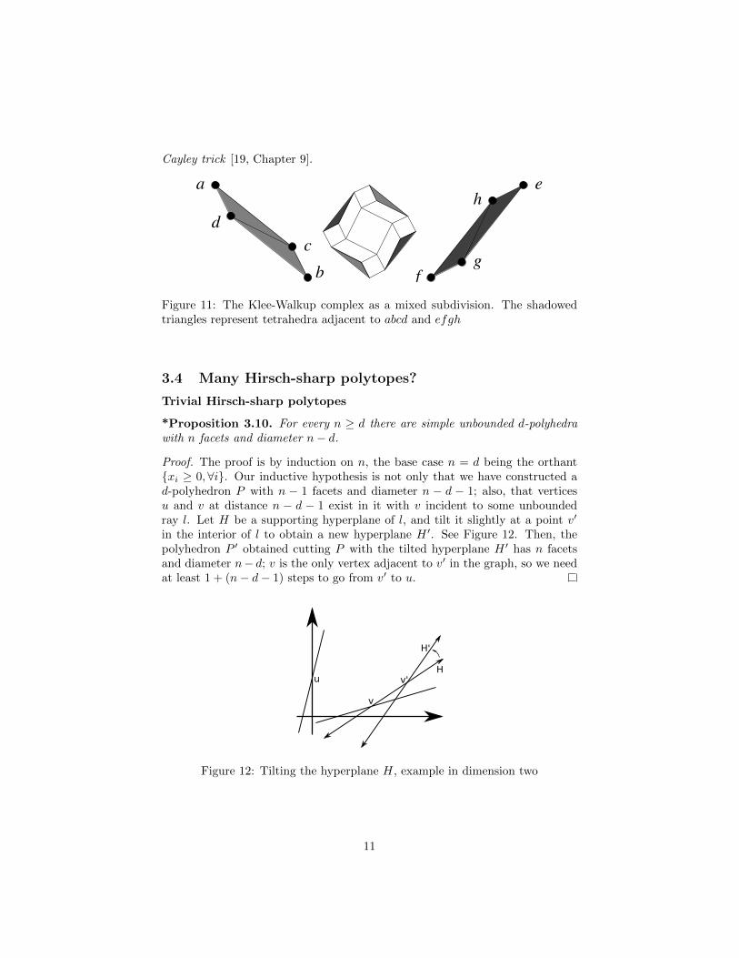
Cayley trick [19, Chapter 9].

a

d

c

b f

eh

g

Figure 11: The Klee-Walkup complex as a mixed subdivision. The shadowedtriangles represent tetrahedra adjacent to abcd and efgh

3.4 Many Hirsch-sharp polytopes?

Trivial Hirsch-sharp polytopes

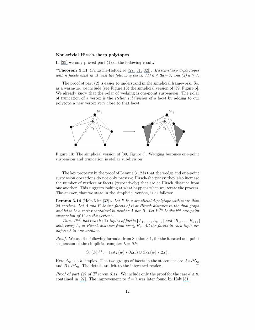
*Proposition 3.10. For every n ≥ d there are simple unbounded d-polyhedrawith n facets and diameter n− d.

Proof. The proof is by induction on n, the base case n = d being the orthant{xi ≥ 0,∀i}. Our inductive hypothesis is not only that we have constructed ad-polyhedron P with n − 1 facets and diameter n − d − 1; also, that verticesu and v at distance n − d − 1 exist in it with v incident to some unboundedray l. Let H be a supporting hyperplane of l, and tilt it slightly at a point v′

in the interior of l to obtain a new hyperplane H ′. See Figure 12. Then, thepolyhedron P ′ obtained cutting P with the tilted hyperplane H ′ has n facetsand diameter n− d; v is the only vertex adjacent to v′ in the graph, so we needat least 1 + (n− d− 1) steps to go from v′ to u.

Figure 12: Tilting the hyperplane H, example in dimension two

11

Non-trivial Hirsch-sharp polytopes

In [39] we only proved part (1) of the following result:

*Theorem 3.11 (Fritzsche-Holt-Klee [27, 31, 32]). Hirsch-sharp d-polytopeswith n facets exist in at least the following cases: (1) n ≤ 3d−3; and (2) d ≥ 7.

The proof of part (2) is easier to understand in the simplicial framework. So,as a warm-up, we include (see Figure 13) the simplicial version of [39, Figure 5].We already know that the polar of wedging is one-point suspension. The polarof truncation of a vertex is the stellar subdivision of a facet by adding to ourpolytope a new vertex very close to that facet.

1

w

1

2 2w

ww

Figure 13: The simplicial version of [39, Figure 5]. Wedging becomes one-pointsuspension and truncation is stellar subdivision

The key property in the proof of Lemma 3.12 is that the wedge and one-pointsuspension operations do not only preserve Hirsch-sharpness; they also increasethe number of vertices or facets (respectively) that are at Hirsch distance fromone another. This suggests looking at what happens when we iterate the process.The answer, that we state in the simplicial version, is as follows:

Lemma 3.14 (Holt-Klee [32]). Let P be a simplicial d-polytope with more than2d vertices. Let A and B be two facets of it at Hirsch distance in the dual graphand let w be a vertex contained in neither A nor B. Let P (k) be the kth one-pointsuspension of P on the vertex w.

Then, P (k) has two (k+1)-tuples of facets {A1, . . . , Ak+1} and {B1, . . . , Bk+1}with every Ai at Hirsch distance from every Bi. All the facets in each tuple areadjacent to one another.

Proof. We use the following formula, from Section 3.1, for the iterated one-pointsuspension of the simplicial complex L = ∂P :

Sw(L)(k) := (astL(w) ∗ ∂∆k) ∪ (lkL(w) ∗∆k).

Here ∆k is a k-simplex. The two groups of facets in the statement are A ∗ ∂∆k

and B ∗ ∂∆k. The details are left to the interested reader.

Proof of part (2) of Theorem 3.11. We include only the proof for the case d ≥ 8,contained in [27]. The improvement to d = 7 was later found by Holt [31].

12

Both are based on a new operation on polytopes that we now introduce. Theversion for simple polytopes is called blending, but we describe it for simplicialpolytopes and call it glueing. Glueing is simply a combinatorial/geometric ver-sion of the connected sum of topological manifolds. Let P1 and P2 be twosimplicial d-polytopes and let F1 and F2 be respective facets. The manifoldsare ∂P1 and ∂P2 (two (d−1)-spheres); from them we remove the interiors of F1

and F2 after which we glue their boundaries. See Figure 14, where the operationis performed on two facets of the same polytope. On the top part we glue thepolytopes “as they come”, which does not preserve convexity. But if projectivetransformations are made on P1 and P2 that send points that are close to F1

and F2 to infinity, then the glueing preserves convexity, so it yields a polytopethat we denote P1#P2. This is shown on the bottom part of the Figure.

F

1

1 22F

P P2

111

22P

P

Figure 14: Glueing two simplicial polytopes along one facet. In the version onthe bottom, a projective transformation is done to P1 and P2 before glueing, toguarantee convexity of the outcome

Glueing almost adds the diameters of the two original polytopes. Supposethat the facets F1 and F2 are at distances δ1 and δ2 to certain facets F ′1 and F ′2of P1 and P2. Then, to go from F ′1 to F ′2 in P1#P2 we need at least (δ1 − 1) +1 + (δ2 − 1) = δ1 + δ2 − 1 steps.

But we can do better if we combine glueing with the iterated one-pointsuspension. Consider the simplicial Klee-Walkup 4-polytope Q∗4 described inSection 3.3 and let A and B two facets of it at distance five. Let P ′ be the 4th

one-point suspension of it on the vertex w not contained in A ∪ B. Observethat P ′ has 13 vertices and dimension eight. By the lemma, P ′ has two groupsof five facets {A1, . . . , A5} and {B1, . . . , B5} with every Ai at Hirsch distancefrom every Bi and all the facets in each group adjacent to one another.

We now glue several copies of P ′ to one another, a Bi from each copy gluedto an Ai of the next one. Each glueing adds five vertices and, in principle, four

13

to the diameter. But Lemma 3.14 implies the following nice property for P ′:half of the eight facets adjacent to each Ai are at distance four to half of thefacets adjacent to each Bi. Using the language of Fritzsche, Holt and Klee, wecall those facets the slow neighbors of each Ai or Bi, and call the others fast.Since half of the total neighbors are slow, we can make all glueings so that everyfast neighbor is glued to a slow one and vice-versa. This increases the diameterby one at every glueing, and the result is Hirsch-sharp.

The above construction yields Hirsch-sharp 8-polytopes with 13+5k vertices,for every k ≥ 0. We can get the intermediate values of n too, via truncation.By Lemma 3.12, every time we do a one-point suspension on a Hirsch-sharpsimplicial polytope we can increase the number of facets by one or two via astellar subdivision at each end. Since the polytope P ′ we are glueing is a 4-foldone-point suspension, and since there are two ends that remain unglued (theA-face of the first copy and the B-face of the last) we can do up to eight stellarsubdivisions to it and still preserve Hirsch-sharpness.

3.5 The unbounded and monotone Hirsch conjectures arefalse

*Theorem 3.16 (Todd [57]). There is a simple bounded polytope P , two ver-tices u and v of it, and a linear functional φ such that:

1. v is the only maximal vertex for φ.

2. Any edge-path from u to v and monotone with respect to φ has length atleast five.

Proof. Let Q4 be the Klee-Walkup polytope. Let F be the same “ninth facet”as in the previous proof, one that is not incident to the two vertices u and vthat are at distance five from each other. Let H2 be the supporting hyperplanecontaining F and let H1 be any supporting hyperplane at the vertex v. Finally,let H0 be a hyperplane containing the (codimension two) intersection of H1 andH2 and which lies “slightly beyond H1”, as in Figure 15. (Of course, if H1 andH2 happen to be parallel, then H0 is taken to be parallel to them and closeto H1.) The exact condition we need on H0 is that it does not intersect Q4

and the small, wedge-shaped region between H0 and H1 does not contain theintersection of any 4-tuple of facet-defining hyperplanes of Q4.

We now make a projective transformation π that sends H0 to be the hyper-plane at infinity. In the polytope Q′4 = π(Q4) we “remove” the facet F ′ = π(F )that is not incident to the two vertices u′ = π(u) and v′ = π(v). That is, weconsider the polytope Q′′4 obtained from Q′4 by forgetting the inequality thatcreates the facet F ′ (see Figure 15 again). Then Q′′4 will have new vertices notpresent in Q′4, but it also has the following properties:

1. Q′′4 is bounded. Here we are using the fact that the wedge between H0

and H1 contains no intersection of facet-defining hyperplanes: this impliesthat no facet of Q′′4 can go “past infinity”.

14

H’π

uv

FH

H0

2

H1

H’1v’

2

u’

Figure 15: Disproving the monotone Hirsch conjecture

2. It has eight facets: four incident to u′ and four incident to v′.

3. The functional φ that is maximized at v′ and constant on its supportinghyperplane H ′1 = π(H1) is also constant on H ′2 = π(H2), and u′ lies onthe same side of H ′1 as v′.

In particular, no φ-monotone path from u′ to v′ crosses H ′1, which means itis also a path from u′ to v′ in the polytope Q′4, combinatorially isomorphic toQ4.

3.6 The topological Hirsch conjecture is false

*Theorem 3.18 (Mani-Walkup [46]). There is a triangulated 3-sphere with16 vertices and without the non-revisiting property. Wedging on it eight timesyields a non-Hirsch 11-sphere with 24 vertices.

Proof. The key part of the construction is the two-dimensional simplicial com-plex K consisting of the following 32 triangles:

amr mbr bnr ncr cor odr dpr paramt mbt bnt nct cot odt dpt pat

aoq obq bpq pcq cmq mdq dnq naqaos obs bps pcs cms mds dns nas

The first and second halves are topological 2-spheres, triangulated in the formof double pyramids over the octagons ambncodp and aobpcmdn (same vertices,but in different order). Observe that in both octagons every edge goes from one

15

om

n

s

q

p

a

b c

d

r

t

n

om

pa

b c

d

Figure 16: Two octagonal bipyramids

of {a, b, c, d} to one of {m,n, o, p}, but the vertices are shuffled in such a waythat no edge is repeated. See Figure 16.

The interiors of the two bipyramids can easily be triangulated (subdividedinto terahedra) in such a way that the tetrahedron abcd is used in the firstone and mnop in the second. Then the two bipyramids can be embedded inthe 3-sphere (with corresponding vertices identified) by first embedding themdisjointly and then pinching the vertices of one of the octagons to glue themwith those of the other. We claim that no extension of this partial triangulationto the whole 3-sphere can have the non-revisiting property.

Indeed, every path from the tetrahedron abcd to the tetrahedron mnop mustexit the first bipyramid through one of its boundary triangles, which uses oneof the edges of the first octagon. In particular, our path will at this pointhave abandoned three of the vertices of abcd and be using one of mnop. Tokeep the non-revisiting property, the abandoned vertices should not be usedagain, and the new one should not be abandoned, since it is a vertex of ourtarget tetrahedron. But then it is impossible for our path to enter the secondbipyramid: it should do so via a triangle using an edge of the second octagon,and non-revisiting implies that this edge should be the same used to exit the firstbipyramid. This is impossible since the two octagons have no edge in common.

We skip the technical part of the proof, namely that K can be completed toa triangulation of the 3-sphere using the tetrahedra abcd and mnop (and withonly four extra vertices). The way Mani and Walkup show it is by listing thetetrahedra of the whole triangulation and verifying that they form a shellablesphere.

16

References

[1] A. Altshuler. The Mani-Walkup spherical counterexamples to the Wv-pathconjecture are not polytopal. Math. Oper. Res., 10(1):158–159, 1985.

[2] A. Altshuler, J. Bokowski, and L. Steinberg. The classification of simplicial 3-spheres with nine vertices into polytopes and non-polytopes. Discrete Math.,31:115–124, 1980.

[3] M. L. Balinski. On the graph structure of convex polyhedra in n-space.Pacific J. Math., 11:431–434, 1961.

[4] M. L. Balinski. The Hirsch conjecture for dual transportation polyhedra.Math. Oper. Res., 9(4):629–633, 1984.

[5] D. Barnette. Wv paths on 3-polytopes. J. Combinatorial Theory, 7:62–70,1969.

[6] M. Beck, S. Robins, Computing the continuous discretely. Integer-point enu-meration in polyhedra. Undergraduate Texts in Mathematics. Springer, 2007.

[7] A. Bjorner, F. Brenti, Combinatorics of Coxeter Groups, Graduate Texts inMathematics, 231, Springer-Verlag, 2005.

[8] L. Blum, F. Cucker, M. Shub, and S. Smale, Complexity and real computa-tion, Springer-Verlag, 1997.

[9] K. H. Borgwardt, The Average Number of Steps Required by the SimplexMethod Is Polynomial. Zeitschrift fur Operations Research, 26:157–77, 1982.

[10] S. Boyd and L. Vandenberghe. Convex Optimization. Cambridge UniversityPress, Cambridge, 2004.

[11] D. Bremner, A. Deza, W. Hua, and L. Schewe. More bounds on the diame-ter of convex polytopes: ∆(4, 12) = ∆(5, 12) = ∆(6, 13) = 7. (in preparation)

[12] D. Bremner and L. Schewe. Edge-graph diameter bounds for convex poly-topes with few facets.

[13] G. Brightwell, J. van den Heuvel, and L. Stougie. A linear bound on thediameter of the transportation polytope. Combinatorica, 26(2):133–139, 2006.

[14] W. H. Cunningham. Theoretical properties of the network simplex method.Math. Oper. Res., 4:196–208, 1979.

[15] G. B. Dantzig, Linear programming and extensions, Princeton UniversityPress, 1963.

[16] J. A. De Loera, E. D. Kim, S. Onn, and F. Santos. Graphs of transportationpolytopes. J. Combin. Theory Ser. A, 116(8):1306–1325, 2009.

17

[17] J. A. De Loera. The many aspects of counting lattice points in polytopes.Math. Semesterber. 52(2):175–195, 2005.

[18] J. A. De Loera and S. Onn. All rational polytopes are transportationpolytopes and all polytopal integer sets are contingency tables. In Lec. Not.Comp. Sci., volume 3064, pages 338–351, New York, NY, 2004. Proc. 10thAnn. Math. Prog. Soc. Symp. Integ. Prog. Combin. Optim. (Columbia Uni-versity, New York, NY, June 2004), Springer-Verlag.

[19] J. A. De Loera, J. Rambau, F. Santos, Triangulations: Applications, Struc-tures and Algorithms. Algorithms and Computation in Mathematics (to ap-pear).

[20] J.-P. Dedieu, G. Malajovich, and M. Shub. On the curvature of the centralpath of linear programming theory. Found. Comput. Math. 5:145–171, 2005.

[21] A. Deza, T. Terlaky, and Y. Zinchenko. Central path curvature anditeration-complexity for redundant Klee-Minty cubes. Adv. Mechanics andMath., 17:223–256, 2009.

[22] A. Deza, T. Terlaky, and Y. Zinchenko. A continuous d-step conjecture forpolytopes. Discrete Comput. Geom., 41:318–327, 2009.

[23] A. Deza, T. Terlaky, and Y. Zinchenko. Polytopes and arrangements: Di-ameter and curvature. Oper. Res. Lett., 36(2):215–222, 2008.

[24] M. Dyer and A. Frieze. Random walks, totally unimodular matrices, anda randomised dual simplex algorithm. Math. Program., 64:1–16, 1994.

[25] F. Eisenbrand, N. Hahnle, A. Razborov, and T. Rothvoß. Diameter ofPolyhedra: Limits of Abstraction. 2009. (in preparation)

[26] S. Fomin and A. Zelevinsky. Y -systems and generalized associahedra. Ann.of Math. 158(2), 977–1018, 2003.

[27] K. Fritzsche and F. B. Holt. More polytopes meeting the conjectured Hirschbound. Discrete Math., 205:77–84, 1999.

[28] E. Gawrilow, M. Joswig. Polymake: A software package for analyzingconvex polytopes. Software available at http://www.math.tu-berlin.de/

polymake/

[29] D. Goldfarb and J. Hao. Polynomial simplex algorithms for the minimumcost network flow problem. Algorithmica, 8:145–160, 1992.

[30] P. R. Goodey. Some upper bounds for the diameters of convex polytopes.Israel J. Math., 11:380–385, 1972.

[31] F. B. Holt. Blending simple polytopes at faces. Discrete Math., 285:141–150, 2004.

18

[32] F. Holt and V. Klee. Many polytopes meeting the conjectured Hirschbound. Discrete Comput. Geom., 20:1–17, 1998.

[33] C. Hurkens. Personal communication, 2007.

[34] G. Kalai. A subexponential randomized simplex algorithm. In Proceedingsof the 24th annual ACM symposium on the Theory of Computing, pages 475–482, Victoria, 1992. ACM Press.

[35] G. Kalai. Online blog http://gilkalai.wordpress.com. See for examplehttp://gilkalai.wordpress.com/2008/12/01/a-diameter-problem-7/,December 2008.

[36] G. Kalai and D. J. Kleitman. A quasi-polynomial bound for the diameterof graphs of polyhedra. Bull. Amer. Math. Soc., 26:315–316, 1992.

[37] N. Karmarkar. A new polynomial time algorithm for linear programming.Combinatorica, 4(4):373–395, 1984.

[38] L. G. Hacijan. A polynomial algorithm in linear programming. (in Russian)Dokl. Akad. Nauk SSSR, 244(5):1093–1096, 1979.

[39] E. D. Kim, and F. Santos. An update on the Hirsch conjecture, preprint2009, version 2. http://arxiv.org/abs/0907.1186v2.

[40] V. Klee. Paths on polyhedra II. Pacific J. Math., 17(2):249–262, 1966.

[41] V. Klee, P. Kleinschmidt, The d-Step Conjecture and Its Relatives, Math-ematics of Operations Research, 12(4):718–755, 1987.

[42] V. Klee, G. J. Minty, How good is the simplex algorithm?, in Inequalities,III (Proc. Third Sympos., Univ. California, Los Angeles, Calif., 1969; ded-icated to the memory of Theodore S. Motzkin), Academic Press, New York,1972, pp. 159–175.

[43] V. Klee and D. W. Walkup. The d-step conjecture for polyhedra of dimen-sion d < 6. Acta Math., 133:53–78, 1967.

[44] P. Kleinschmidt and S. Onn. On the diameter of convex polytopes. DiscreteMath., 102(1):75–77, 1992.

[45] D. G. Larman. Paths of polytopes. Proc. London Math. Soc., 20(3):161–178, 1970.

[46] P. Mani and D. W. Walkup. A 3-sphere counterexample to the Wv-pathconjecture. Math. Oper. Res., 5(4):595–598, 1980.

[47] J. Matousek, M. Sharir, and E. Welzl. A subexponential bound for linearprogramming. In Proceedings of the 8th annual symposium on ComputationalGeometry, pages 1–8, 1992.

19

[48] N. Megiddo. Linear programming in linear time when the dimension isfixed. J. Assoc. Comput. Mach., 31(1):114–127, 1984.

[49] N. Megiddo. On the complexity of linear programming. In: Advances ineconomic theory: Fifth world congress, T. Bewley, ed. Cambridge UniversityPress, Cambridge, 1987, 225-268.

[50] D. Naddef. The Hirsch conjecture is true for (0, 1)-polytopes. Math. Pro-gram., 45:109–110, 1989.

[51] T. Oda, Convex bodies and algebraic geometry, Springer Verlag, 1988.

[52] J. B. Orlin. A polynomial time primal network simplex algorithm for min-imum cost flows. Math. Program., 78:109–129, 1997.

[53] J. Renegar. A Mathematical View of Interior-Point Methods in ConvexOptimization. SIAM, 2001.

[54] S. Smale, On the Average Number of Steps of the Simplex Method of LinearProgramming. Mathematical Programming, 27: 241-62, 1983.

[55] S. Smale, Mathematical problems for the next century. Mathematics: fron-tiers and perspectives, pp. 271–294, American Mathematics Society, Provi-dence, RI (2000).

[56] D. A. Spielman and S. Teng. Smoothed analysis of algorithms: Why thesimplex algorithm usually takes polynomial time. J. ACM, 51(3):385–463,2004.

[57] M. J. Todd. The monotonic bounded Hirsch conjecture is false for dimen-sion at least 4, Math. Oper. Res., 5:4, 599–601, 1980.

[58] R. Vershynin. Beyond Hirsch conjecture: walks on random polytopes andsmoothed complexity of the simplex method. In IEEE Symposium on Foun-dations of Computer Science, volume 47, pages 133–142. IEEE, 2006.

[59] D. W. Walkup. The Hirsch conjecture fails for triangulated 27-spheres.Math. Oper. Res., 3:224-230, 1978.

[60] G. M. Ziegler, Lectures on polytopes, Graduate Texts in Mathematics,152, Springer-Verlag, 1995.

[61] G. M. Ziegler, Face numbers of 4-polytopes and 3-spheres. Proceedingsof the International Congress of Mathematicians, Vol. III (Beijing, 2002),Higher Ed. Press, Beijing, 2002, pp. 625–634.

Edward D. Kim

Department of MathematicsUniversity of California, Davis. Davis, CA 95616, USA

20

email: ekim@math.ucdavis.edu

web: http://www.math.ucdavis.edu/~ekim/

Francisco Santos

Departamento de Matematicas, Estadıstica y ComputacionUniversidad de Cantabria, E-39005 Santander, Spainemail: francisco.santos@unican.es

web: http://personales.unican.es/santosf/

21

Contents

1 Introduction 1

2 Bounds and algorithms 12.1 Small dimension or few facets . . . . . . . . . . . . . . . . . . . . 12.2 General upper bounds on diameters . . . . . . . . . . . . . . . . 32.4 Some polytopes from combinatorial optimization . . . . . . . . . 52.5 A continuous Hirsch conjecture . . . . . . . . . . . . . . . . . . . 5

3 Constructions 63.1 The wedge operation . . . . . . . . . . . . . . . . . . . . . . . . . 63.2 The d-step and non-revisiting conjectures . . . . . . . . . . . . . 73.3 The Klee-Walkup polytope Q4 . . . . . . . . . . . . . . . . . . . 83.4 Many Hirsch-sharp polytopes? . . . . . . . . . . . . . . . . . . . 113.5 The unbounded and monotone Hirsch conjectures are false . . . . 143.6 The topological Hirsch conjecture is false . . . . . . . . . . . . . 15

22