1

The Coase Conjecture in Continuous Time:Imperfect Durability, Endogenous Durability, and Aftermarkets

April 10, 1996Bruce W. Hamilton and Mary Burke

INTRODUCTION

With the exceptions of Bond and Samuelson (B&S) (1984) and Bulow (1986), the

extensive literature on the Coase (1972) conjecture deals only with goods of infinite durability.

As Coase argued, in a continuous time setting where the monopolist can change price without

notice, price instantly falls to marginal cost if the good is infinitely durable. But we know little

about how this intuition carries over to limited durability, which is the case with virtually all real-

world goods. Stokey (1981) introduced two analytical tools to the Coase discussion: (i) perfect

rational-expectations equilibrium (PREE), and (ii) discrete time in the form of a "trading period,"

a repeated exogenous time interval during which the monopolist is unable to cut the price.

A PREE is a time-consistent profit-maximizing time path of production, subject to the

restriction that consumers’ expectations regarding future output be always realized, and

furthermore that following any perturbation from the profit-maximizing path, expectations will

continue to be realized along the new profit-maximizing path.

Stokey shows that with perfect durability and continuous time, the only PREE is instant

market saturation, as Coase had originally argued.

This leads Stokey to introduce the trading period. Sure enough, by partially restoring the

commitment power which Coase had taken away from his monopolist, monopoly profit is partially

restored. The longer the trading period, the greater is the restoration. Stokey finds that price

brought to you by COREView metadata, citation and similar papers at core.ac.uk

provided by Research Papers in Economics

2

As we will show, trading periods must be quite long (in the range of a year or more) in1

order to have much of a damping effect on the Coase discipline.

By "continuous time," we mean that the firm has the power to cut price at any instant,2

regardless of his history of prior price cuts.

approaches marginal cost, after a sufficient number of trading periods has elapsed,regardless of

the length of the individual trading period (denoted as z).

The literature offers no economic rationale for the trading period, nor any plausible

mechanism whereby a monopolist can credibly precommit to a trading period. Neither Stokey1

nor any subsequent author offers a serious discussion of where the trading period comes from.

Thus the literature leaves us with the twin artificial constructs of infinite durability and a finite

(and quite long) trading period.

Note in particular that menu or price-adjustment costs would not give rise to a finite

trading period. Menu costs, once incurred, are sunk, and ex post the firm will want to cut price

immediately after sales have dried up from the previous price cut (i.e., in the twinkling of an eye).

We believe it is more fruitful to retain Coase’s reasonable assumption of continuous time2

and relax the unreasonable assumption of infinite durability, rather than the other way around.

Our goods are of limited durability, and time is continuous; the firm is given no free commitment

power with which to save itself from time inconsistency. In Part I, the durability of the good is

exogenous. We find that the firm retains substantial monopoly power except for very durable

goods, even without the free commitment power given by discrete time.

In Part II, the level of durability is set by the monopolist. Given the negative relationship

between durability and ability to retain monopoly power, this monopolist cuts durability below its

efficient level to save itself from the Coase temptation. As a result it produces the good in a

3

(1)

technically inefficient manner and recovers much of the monopoly profit that it would have lost

had durability been exogenous. As Bulow (1986) noted in a two-period setting, the Swan (1972)

independence result breaks down in the presence of the Coase temptation.

In Part III we consider the important case in which the lifetime of the good is jointly

determined by built-in durability (as in Part II, above) and consumers’ maintenance decisions (as in

Schmalensee (1974) and Rust (1986)). In this setting we deal specifically with the case in which

the monopolist has power not only over the original equipment but also over some

replacement/repair parts. We find that the monopolist charges a much higher markup on parts

than on original equipment. To a good approximation, he escapes the Coase temptation by

pricing the durable good at marginal cost (giving in to the temptation) and taking a high markup

on the flow demand for parts. Power over parts further restores the sales monopolist’s credibility

and profit, at the cost of a still more inefficient production plan.

Within real-world ranges of durability, even without a trading period, we find no plausible

circumstance in which the durable-goods sales monopolist behaves approximately competitively.

Durability gives no reason to believe that monopoly is benign; "competition from installed base"

should not be accepted as a part of an antitrust defense.

I. EXOGENOUS DURABILITY

Consider a product which lasts for a timespan d and then dies like the one-hoss shay. Unit

production cost is C. Inverse demand for the service flow is

m

m

xt

X q x dtt t tt d

d

t d

t= +

−− ∫∑

4

(2)

(3)

Without physical depreciation (until death at d), X is the aggregate of production over thet

timespan from t-d to t:

where X is the stock and x is the flow. The firm chooses a path of x tot t t

subject to the time-consistency requirement that at each future date the remaining path be optimal.

p is the price of the good at time J, which is in turn the present value of consumers’ expectedJ

future R(X).

Definitions

: the instantaneous rate of production at time t.

q : an instantaneous production $spike# at time tt

X : the stock of the good at time t.t

H : the history of production from t-d to t; i.e., the age distribution of the standing stock.t

( )G s t H x q H s tt s s t, , , | ;= ∀ >

Hx x t

q t

x x t

q t

0

0

0 0

0

0 0

== ∀ ≤= ∀ ≤

= ∀ >= ∀ >

$

;

$

5

Expectations

Under infinite durability, or exponential-decay depreciation, X is a sufficient statistic fort

H ; the age distribution of the stock is irrelevant. But under one-hoss-shay depreciation, the aget

of the stock matters; a given stock age d-, is not the same as the same stock age ,, though both

stocks yield the same service at time t. Consumers’ expectations for future production must be

conditioned on the age distribution of the stock, H, not just the scalar X. They form expectations

rationally; that is, they expect the firm to maximize future profits, subject to a time consistency

constraint. Expectations are represented as

As in Stokey, we require expectations to be consistent; if expectations up to time s are realized,

then expected production at time s is not revised.

Proposition 1: There is a unique Rational-Expectations Steady State (RESS), given the cost

and demand parameters of the problem. A RESS is a production plan of the following form:

A steady state is a smooth age distribution over all relevant History, and for all future time. The

proposition states that there exists a steady state, characterized by the constant flow rate x*, such

6

(4)

(5)

that if the rate x* has persisted from t = -d to t = 0, the firm will not deviate from this production

rate in the future.

Following Stokey, we specify (point) expectations as follows:

where G(@) defines consumers’ expected stock at any future date s, as of time t, given the time-t

stock, X . The trading period z disappears from the function since it is equal to zero. t

The typical research strategy at this stage of the analysis is to pick a functional form for

G(@) and solve for its parameters. Generally (following Stokey) the form is postulated to be

that is, a constant fraction of the gap between current and limiting stock is closed in each trading

period. X& is the limiting stock which the monopolist approaches asymptotically. The model can

then be solved for µ and X&, the rate of adjustment and the limiting stock.

Note that there is nothing "rational" about consumers' choice of the functional form (5);

therefore, the solutions to these models are not necessarily unique nor even very plausible. The

choice of the G(@) functional form is a more serious matter than, for example, choosing a

functional form for a demand function. As we argue below, at least in the case of continuous time

rationality itself dictates the functional form for G.

In continuous time, faced with rational consumers, the firm cannot extract any profit by

holding X below the limiting stock, even for the twinkling of an eye. This of course is the original

Coase insight. Thus, in continuous time, the only functional form for G(@) consistent with

7

Note that this is true in both Coase and continuous-time Stokey. Without a trading3

period, the only thing to solve for is X&. Indeed, Coase’s original insight, though not expressed inquite these terms, is that (6) is the only functional form consistent with rationality in continuoustime.

(6)

rationality is the first line of (6):

To see this, suppose X < X&. If the firm were to close only part of the gap in the first instant

(hoping to keep the price up), it would be tempted to close more of the gap in the next instant.

Consumers, knowing both X& and the firm’s inability to commit, wait a few instants. Thus p(X) =

p(X&) é X so the monopolist maximizes profit by immediately setting X = X&. So (6) (top line) is

the only rational expectations function in continuous time. Clearly, then, the continuous-time

rational consumer’s only problem is to solve for X&.3

Expectations when X $ X&

Now note the second line of (6), which defines expectations if current stock exceeds X&.

In Stokey, and in Bond and Samuelson, expectations are simply not defined if X > X&.

Algebraically, (5) implies that stock gradually shrinks if X should be perturbed to a point beyond

X&, but in the case of perfect durability this is impossible; the stock never dies. And in the case of

imperfect durability, satisfying (5) may also be impossible, since the implied rate of decline in the

stock might exceed the rate at which the stock depreciates. In the Stokey-inspired literature,

equilibria are only perfect "from below;" the equilibria are simply not defined if X > X&. Of course,

profit-maximizing behavior never takes us into this range; nevertheless, perfection of the

8

(7)

equilibrium requires that we tidy this detail.

In the range where X > X&, we assume static expectations: consumers believe that if the

firm somehow does push X beyond X&, it will not further expand the stock. For their part, of

course, firms would not find it profitable to further expand the stock given consumers’

expectations. The firm might, however, wish to shrink the stock. We rule this out by assuming

the firm never conducts "sales." Price cuts, once announced, are irreversible. Given this

assumption, static expectations are rational in the range X > X&; once the firm has inadvertently

overshot X&, the best it can do is to refrain from expanding further. In the appendix we discuss

the rationale for the no-sales assumption; here we simply note that this assumption is present,

though unstated, in all of the Coase literature, and that we adopt it explicitly.

In fact we make virtually no use of the expectations assumption in the region X > X&.

Equilibrium does not occur in this region, nor does any equilibrium path of output enter it

(starting from any X # X&). And no starting point, X # X&, generates consumer expectations that X

will ever exceed X&.

Solving for X&

If (6) is ex post correct for all time, then consumers must have solved for it at t = 0.

Consumers approach this problem as follows: Consider a candidate stock, X*; is it X&? Let us

suppose that X* has been maintained by a constant flow of production,

m

9

(8)

(9)

(10)

(11)

The age distribution is uniform; if future production is held at x * the stock will remain fixed atJ

X*. Suppose the firm contemplates a small deviation from x *, increasing output above X*. InJ

particular, the firm contemplates a production spike, x**, at t = 0, t = d, t = 2d, etc. This instantly

raises the stock to X*+x** and holds it there in perpetuity. X* = X& if a small increase in stock,

x**, is not profitable. Thus we (and consumers) solve for X& by finding that value of X from

which a small permanent increase is not profitable, given expectations. The firm’s value at t is

where (@) is the discounted flow of future production, [@] is the consumers’ rental price given the

stock (will permanently be) X*+x**, and

is the present value operator for the timespan d. Thus [@]@ b(D,d) = price.

X& is that X at which

The solution is

10

(12)

where the arguments D and d are henceforth suppressed in b(D,d) for compactness.

The competitive and rental-monopoly outputs are characterized by analogs to (11):

Proposition 1:

� As d 6 4, X& 6 X& .S C

� As d 6 0, X& 6 X&S R

Proof:

X& /X& depends only upon d and D; Figure 1 shows X& /X& (d) respectively for D = .05 andS R S R

0.10. Note in particular that monopoly output remains quite low even for product lifetimes as

11

The question we pose is essentially identical to that of Bond and Samuelson, but our4

results are strikingly different. In the Appendix we show how and why our results differ fromtheirs.

high as 15 to 20 years. For any real-world durable good, even in continuous time, monopoly

power remains significant for a sales monopolist.

Figure 1 depends only minimally on functional forms; the only arbitrary functional form is

the assumed linearity of the demand function. The message is stark and clear: The Coase

temptation offers only modest relief to consumers, for goods with less than about a 15-year

lifetime.4

Recall that the PREE is found by solving (10). It is worth noting that (10), in addition to

being our solution method, is a natural characterization of the rational and informed consumer’s

decision-making problem: When faced with a stock of X*, the consumer’s natural question is this:

"Has the Coase force spent itself, or will the firm raise X above X* in the next instant?" When

(10) is satisfied, the consumer knows that the Coase force can offer him no more help.

II ENDOGENOUS DURABILITY

So long as durability is exogenous, welfare and consumers’ utility unambiguously rise

when rental-only is prohibited (as in current antitrust enforcement), though the welfare

improvement is much more modest than the literature suggests. As shown above, and illustrated

in Figure 1, a sales monopolist enjoys considerable monopoly profit even if its product lasts 15 to

20 years. Nevertheless, such a firm, while still enjoying profit, loses substantial profit to Coase.

If D = .05 and d = 20 years, the sales monopolist loses approximately 40% of potential profit to

Coase. In this section we explore the possibility that a sales monopolist reduces durability to

recapture his power over Coase.

12

(14)

(15)

(16)

(17)

Suppose production cost is given by

where C is unit cost, and c is the cost of added durability. Socially optimal durability (which is1

produced by both the rental monopolist and the competitive industry) requires

Assume now that the monopolist can commit to a given level of d; his problem is to

decide on the level of d, knowing that d influences not only the cost of producing the service flow

(optimized in equ. (15)) but also his ability to withstand the Coase temptation. For any given

level of durability, sales-monopoly flow of output is

(derived above in equation (11)) and the flow of profit is given by

Differentiating equation (17) with respect to d and setting = 0,

13

(18)

(19)

(20)

where x’ = Mx/Md (the derivative of (16) with respect to d):

The expression inside [] in equations (18) and (19) is the net reduction in cost of

producing service flow as d is increased. For compactness, henceforth [] = H (where H stands

for efficiency gain from added durability). MH/Md < 0 and H = 0 for optimal durability. Thus if H

> 0, durability is less than optimal. It is now straightforward (but messy) to show that H > 0 for

the sales monopolist. Substituting (19) into (18) and rearranging:

Hence H > 0, confirming that the sales monopolist produces less than optimal durability.

In principle, we can solve (20) for d, and from that solve for the monopolist’s steady-state

output and profit. However, this expression is very unwieldy and gives little insight into behavior.

14

Unlike many numerical results, this work can readily be reproduced on a simple5

spreadsheet program. For d from 1 to 100, calculate x(d) in equ. (16) on a spreadsheet, forvarious parameter values. Substitute into (17), giving maximum profit as a function of d. Sincethe firm can commit to any d, the value of d at which profit is maximized is the equilibrium. Choice of d takes account of lost Coase immunity as d rises, as well as the effect of d onproduction cost.

On the other hand, it is very easy to obtain numerical results.5

Numerical Solutions

Figure 2 shows the profit-durability relationship for a sales and rental monopolist

respectively, for the parameter values given in Column 1 of Table 2. For every d, sales profit is

lower than rental, because of the Coase temptation. And as discussed above, the (percentage)

gap rises with d. The sales monopolist’s profit reaches its maximum at a lower d than does the

rental monopolist’s, representing the sales monopolist’s (partial) escape from Coase by cutting d.

Numerical results, for a variety of parameter values, are given in Table 2 below:

Table 2Sales and Rental Monopolywith Endogenous Durability

column 1 2 3 4 5 6 7 8

" 100 200 100 100 100 200 100 100

( 1 1 1 1 1 1 1 1

c0 50 50 50 50 10 100 50 50

c1 20 20 20 5 65 3 0 -10

D .05 .05 .10 .05 .05 .05 .05 .05

dS 5.9 4.4 4.3 6.4 2.2 6.5 6.5 6.9

dR 9.2 9.2 6.3 17.2 2.4 28.1 4 4

V /VS R .833 .861 .771 .790 .94 .766 .470 .410

C /CsS R 1.036 1.101 1.034 1.270 1.00 1.76 3.60 *

X /XS R 1.054 1.034 1.081 1.039 1.025 1.025 1.008 .76

*: C = -3.26; C = -47.82S R

Note: In Col.9, V and X grow without bound as d rises (since cost goes to -4 asR R

d rises). We have set d = 100 for the rental monopolist in Col. 9.

15

First consider Column 1, the parameter values for Figure 2. The sales monopolist reduces

d from its optimal value (9.2 years) to 5.9, raising production cost by 3.6%. Profit is 83.3% that

of the rental monopolist.

Column 2 reveals that raising monopoly power (" = 200) causes the sales monopolist to

deviate further from optimal durability. With greater (potential) profit, the monopolist has a

greater incentive to cut durability. In Column 3 we raise the discount rate to .10; this makes the

sales monopolist more subject to the Coase temptation; it responds by cutting durability more

than when D = .05, and it earns less profit .

In Column 4 we create a very durable good (optimal lifetime = 17.2 years, possibly an

automobile). The sales monopolist sets d = 6.4. Production cost of the service flow is 27%

above optimal. Profit is 79% that of the rental monopolist.

Columns 5 and 6 present extremes of plausible durability. In Column 5 optimal durability

is 2.4 years; the sales monopolist’s behavior is very little different from the rental monopolist’s. In

Column 6, optimal durability is 28.1 years. Were the sales monopolist to produce this durability,

its profit would only be 48% of rental profit. Despite a 76% increase in production (of service

flow) cost, it chooses to cut durability back to 6.5 years, to find a safe harbor from Coase

competition, earning 76% of the rental monopolist’s profit.

In Column 7, production cost is independent of durability (c = 0). The rental monopolist1

obviously produces infinite durability; the sales monopolist still produces a good of 6.5 years’

durability, at a cost 3.6 times that of the rental monopolist.

In Column 8, it is costly to reduce durability; c = -10. Even in this extreme version,1

where at d = 4 C = -4, the sales monopolist produces a good of 6.9 years durability, and earns

16

41% as much profit as the rental monopolist.

Finally note the bottom row, which shows the ratio of sales to rental stock (if the sales

monopolist fully fell victim to Coase, this ratio would be 2). In no case does X /X rise aboveS R

1.088. This crucial ratio remains small for the following reasons:

� If optimal durability is small (say in the range of 5 years) then sales output is not much

higher than rental in any event (an extension of the Part-I finding);

� If optimal durability is high, the sales monopolist tends to cut durability, which depresses

output for two reasons:

i. At lower durability the sales monopolist faces less Coase temptation, and

ii. As durability is reduced, cost is increased, further depressing output.

Thus regardless of whether optimal durability is high or low, sales-monopoly output is

only very slightly above rental output. The results (confirmed by other numerical analyses over a

wide range of parameter values) can be summarized quickly:

� Sales-monopoly durability falls relative to rental when

i. optimal durability rises,

ii. potential monopoly power (the intercept of the demand curve) rises,

iii. the interest rate rises.

In particular, whenever optimal durability is great enough to seriously erode sales-monopoly

profit, durability is cut back dramatically, even if such a cutback is quite costly.

� Sales-monopoly stock, over a very wide range of parameter values, is less than 10%

higher than rental-monopoly stock.

The results of Sections I and II strongly suggest that Coase discipline offers little relief to

17

Some of the most contentious recent antitrust litigation has centered on OEMs’ efforts to6

protect their aftermarkets. See AMI v IBM 93-1586 3rd (1994) and Eastman Kodak Co. v ITS,et al 112 S. Ct. 2072 (1992). IBM and Kodak had each attempted to exclude independent serviceorganizations from performing maintenance and upgrade work on their original equipment(respectively large scale mainframe computers and copiers).

consumers. If durability is exogenous, sales monopolists capture a substantial fraction of rental

monopolist’s profit despite the Coase discipline, so long as durability is not "too great." Certainly

for products with lifetimes of 10 to 15 years, sales monopolists enjoy a substantial fraction of the

profit of rental monopolists. If the monopolist can set durability, it continues to enjoy substantial

monopoly profit even for goods which should last for many decades. It simply reduces the

durability of the good and escapes the Coase temptation.

With endogenous durability, prohibition of rental-only is not generally welfare enhancing.

Though the sales monopolist usually slides a (tiny) bit farther down the demand curve than does

the rental monopolist, he produces the product in an inefficient manner.

III MAINTENANCE

In Sections I and II, the lifetime of the product is determined on the factory floor. But for

an important class of goods, lifetime is jointly determined by built-in durability and maintenance,

which is performed by consumers if the good has been sold, during the lifetime of the good. And

for many such goods, the original equipment manufacturer (OEM) is the sole supplier of some of

the parts and expertise required to maintain the good. In this section we consider the behavior of6

a durable-goods monopolist (respectively sales and rental) which possesses such aftermarket

power. We find that such a monopolist can use its parts-pricing power to recover much of the

power it would otherwise lose to Coase.

18

(21)

(22)

(23)

(24)

A. Technology

Unit cost of producing the durable good is

where a is an index of maintenance required to keep the product alive. The level of maintenance

required at age t is given by

Maintenance, in turn, is produced according to a CES technology:

The inputs are respectively "parts" B, and "service" s. Parts are produced and priced exclusively

by the OEM, and service is marketed competitively.

B. Pricing

The price of original equipment (the product) is

where 2 is the monopolist’s markup over production cost. The price of parts is

19

(25)

(26)

(27)

(28)

(29)

where the cost of manufacturing parts is normalized to unity and N is the markup over cost. The

cost (to the consumer) of maintenance is

where

C. Consumer Behavior

In the PREE, 2, N, a are constant. Given 2, N, a, consumers choose the following:

(1) the mix of parts B and service s in the production of maintenance;

(2) the scrapping age, d, of the product, and

(3) the quantity of the product to purchase.

The consumer’s cost-minimizing mix of maintenance inputs is given by

20

(12) does not yield a closed-form solution for d; the implicit solution is given in equation7

(23) in the Appendix.

(30)

(31)

(32)

Age-0 maintenance expenditure, µ , can thus be expressed as 0

where F = 1/(1+R) is the elasticity of substitution between parts and service in the production of

maintenance, f (@) and f (@) are the two bracketed expressions to the right of a in equation (30),1 2

and f(@) = f @ f .1 2

Next the consumer determines the optimal scrapping age, d.

where the right hand side of (32) is the perpetual rental cost of the product as a function of 8. 7

Having solved for d, rental cost is found by substituting d for 8 in the right hand side of (32):

21

In Sections I and II, consumers’ expectations were defined over X; here we find it more8

convenient to define expectations over prices (and built-in durability, a).

(33)

(34)

(35)

As in Parts I and II, demand for the services of the product is linear in R:

The Perfect Rational Expectations Equilibrium

As above, we analyze a PREE (Perfect Rational Expectations Equilibrium). Formally, we

assume

1. Consumers know all of the parameters of the model;

2. Consumers do not anticipate any "sales;" i.e., price cuts followed by price increases;

3. Time is continuous; the firm is free to change 2,N,a at any time without notice.

As in Parts I and II, there is only one functional form for expectations, consistent with

rationality in continuous time:

Consumers solve for {*} using the same method we employed in Parts I and II: they test

a vector {2",N",a"} for steady-state-ness by solving the firm’s problem:8

22

Derivation of 2*(N,a), N*(2,a), and a*(2,N), and the solution to these expressions, is9

described in the Appendix.

(36)

(37)

The maximization problem is interpreted as follows: {2",N",a"} has persisted for the

relevant past (at least for a timespan d, the lifetime of the good). Calculate the value of the firm,

given this history, assuming that the new vector {2,N,a} will be permanent once announced. If

then {2",N",a"} is {2*,N*,a*}; satisfaction of (37) ensures that no permanent price change from

{2",N",a"} is profitable. Thus {*} is a PREE by the same reasoning employed in parts I and II.

Solving the Model

As in Section II, the model does not yield tractable analytical solutions. Therefore, in this

section we report and discuss numerical values of {2*,N*,a*}.

The problem is solved piecemeal: First hold N and a constant and solve for 2*. Repeat

this operation for a wide range of values of N and a to obtain a relationship 2*(N,a). That is, for

any given N and a, 2*(@) gives the profit-maximizing permanent value for 2. By the same method,

obtain N*(2,a) and a*(2,N). The solution to these three equations is our PREE vector, {*}. 9

In Tables 3 and 4 we present the results from the parameter vector shown. The good is

designed to be similar to that of Column 4 of Table 2. The first row shows the competitive

23

The parts markup is huge for the standard Marshallian reasons: the elasticity of10

substitution between parts and service, and also between maintenance and original equipment, issmall; and parts’ share in the cost of the product’s service is small as well. With differentparameter values the parts markup is smaller.

Crandall, et al (1986) estimate that the price markup on automobile parts is generally 311

to 8 times the markup on automobiles themselves.

outcome; the second shows the rental monopolist’s outcome. Row 3 presents the results for the

sales monopolist with parts power. The original-equipment markup is 2 = .54, and the parts

markup N is 43.84. Cost to the consumer, R, is 3.62% above that for a rental monopolist, and10

d = 8.36 (efficient d = 18.64). Social cost of the service flow is 37% above optimum. The value

of the firm is 92.4% that of the rental monopolist.

Table 3Equilibrium With Aftermarket Power

g=.1; D = .05; c = 50;c = 5;F = 0.1;" = 800;( = 10 1

V R 2 N a d cost

Competition 0 73.75 0 0 .285 18.64 73.75

RentalMonopoly

132132 436.8 .285 18.64 73.75

Sales Monopoly 121128 452.6 0.54 43.48 .277 8.36 101.1

Table 4Rental/Sales Comparisons

X /XS R .957

C /CS R 1.37

V /VS R .917

Note that the sales monopolist takes virtually all of his monopoly profit via the markup on

parts rather than original equipment, because a high parts price is intertemporally credible,

whereas a high original-equipment price is not. The result is a socially excessive markup on11

parts and a too-early scrapping age.

24

The issue was first discussed (and rejected) by Judge Learned Hand in US vs. Alcoa12

(1945) and is the basis for many court rulings requiring OEM’s to sell rather than only lease theirproducts.

Unlike the numerical analysis of Part II, this simulation is extremely tedious; see13

Appendix.

Finally, note that our sales monopolist produces a smaller stock than does the rental

monopolist. Although cost of the flow of services is 37% above optimal, profit is only 8.3%

below that of the rental monopolist.

In virtually all of the Coase literature, the playing of the Coase game reduces deadweight

loss, helps consumers, and harms the firm. Coase is the friend of both efficiency and consumers.

Unfortunately, the aftermarket is a privately effective but socially wasteful anti-Coase weapon.

Consumers may be even worse off than under rental monopoly (as they are in Table 3), and there

is a large waste of resources via early scrappage. The Coase benefit to consumers is

overwhelmed by the sales monopolist’s technically wasteful response to that temptation.

The role of the installed base is intriguing and somewhat surprising. Most antitrust

observers believe that a substantial installed base, not owned by the OEM, serves as a check on

monopoly power. New equipment must compete with this used equipment. But in the presence12

of aftermarket power, a substantial base, even if owned by consumers, is a powerful antidote to

the Coase temptation; it enables the firm to credibly charge a monopoly markup on parts.

Other Parameter Values

We believe that the only tractable approach to this problem is simulation . This of course13

leaves us without analytical solutions, and without the insight into general patterns which

analytical solutions can give. In Part II we presented results for a wide range of parameter values;

25

in Part III we present only the parameter values depicted in the table. The product underlying

Tables 3 and 4 is similar to that of Column 4 in Table 2; it "should" last between 15 and 20 years,

and the sales monopolist cuts it back to somewhere between 7 and 9 years. In other simulations

we have determined that the model of Part III responds to different parameter values in essentially

the same way as that of Part II. Whenever the monopolist of Part II would cut durability, the

monopolist of Part III raises the parts price, which in turn induces the consumer to shorten the life

of the good. Thus for example, when optimal lifetime is long (in excess of about 10 years), the

monopolist faces a substantial Coase threat and reduces durability in the Part-II model or raises

parts prices in the Part-III model. On the other hand, when optimal durability is less than a

decade, the Coase temptation is small in any event, and the monopolist gains little by reducing

durability or setting a disproprotionately high parts price. Monopolistic parts pricing, like

durability reduction, is a weapon to be employed only if Coase losses would otherwise be

substantial.

IV CONCLUSION

This paper explores the characteristics of perfect rational-expectations equilibria for

monopolists producing finitely durable goods in a continuous-time setting. We model this

problem because we believe that both limited durability and continuous ability to change prices

are more realistic than the standard paradigm of infinite durability and discrete (and quite long)

trading periods. Even if durability is exogenous, we find that sales monopolists retain a great deal

of monopoly power, except for goods with lifetimes of several decades or more.

If the monopolist has the power to determine the level of built-in durability, he can further

recover monopoly profit by reducing durability below its optimal level.

26

Finally, if the monopolist has control over the market for repair/replacement parts which

are required to maintain the good, the sales monopolist recovers still more profit.

Since altering built-in durability and excessively raising parts prices result in technical

inefficiency which a rental monopolist would not find necessary, it is possible that consumer

welfare is higher under rental than sales monopoly.

In no plausible case do we find that the Coase discipline comes close to replicating the

welfare benefits of competition, and in many instances it does more harm than good.

27

Appendix

I. Why No Sales?

All of our equilibria are PREE, subject to the restriction that there be no sales. In parts I

and II no-sales gives rational consumers static expectations for X $ X&; in Part III it takes the form

of a restriction that a price cut below 2* be irreversible. The same assumption underlies the

work of Stokey, and of Bond and Samuelson, though it is unstated in their work.

Of course, Stokey’s monopolist would never intentionally let X > X&. In the case of

imperfect durability, however, a monopolist might want to engage in sales; i.e., to capture residual

demand by a temporary price cut. We choose not to analyze sales for the following reasons:

� Our assumption is in keeping with the (unstated) assumption in the rest of the literature;

� We wish to analyze the importance of the Coase force in our setting (imperfect durability

and parts power), and we interpret the Coase force to be the inexorable downward

pressure on price due to the time consistency problem. Regardless of whether there are

occasional sales, the Coase forces will not permanently push stock above X& in Parts I and

II or price below 2* in Part III.

� We are not able to formally characterize a PREE in which sales are permitted. It is not

clear how to model consumers’ expectations in the presence of sales, as we will discuss.

Most important, it is difficult to imagine a plausible predictable pattern of sales in which

anybody buys at the regular price.

� Despite our inability to formally model sales, we offer the following strong informal

reason to believe that sales are unimportant in this context.

First, consider a regular pattern of sales in the world of exogenous durability. In a prior

28

regime without sales, the flow of output has been constant at x*. At time t, the firm begins to

hold sales, hoping to capture residual demand. It is natural to think of these sales as occurring on

the d interval; i.e., to repeat the sale when the residual demanders’ goods die. But nonresidual

demanders will anticipate this pattern of sales and retime their purchases. If d = 10 years and D =

.05, it is easy to show that just over 20% of the in-service stock will be prematurely retired to

take advantage of the sale price. A consumer whose good will require replacement at time t faces

a rental stream of

if he waits and buys at full price. If instead he retires his good early to take advantage of the sale

(and the series of repeat sales which he anticipates on the d interval), his stream is

Setting R = R and solving for t,f s

If d = 10 years, D = .05, and P = .9 P, just over 21% of the stock will be prematurely retired tos

take advantage of the new cycle of sales. And before the second (anticipated) sale many more

29

A "sale" takes the form of a once-only reduction in the markup, 2, on the product.14

consumers will postpone replacement to get onto the sale cycle. Thus it is extremely difficult,

with a pattern of anticipated sales, to target residual demanders and preserve the high price for

replacement demanders. But if replacement demanders buy at the sale price, then the sale price is

the regular price.

Now consider the effect of a once-only unanticipated sale, in the model of a monopolist

with aftermarket power. Assume that consumers recognize that the sale is temporary (as they14

should, if they are rational), and that they expect it never to be repeated. Consequences are:

(1) Sale to residual demanders (the Coase target), and

(2) Early retirement of older installed base to take advantage of the temporary sale price.

The firm must weigh the profit of selling to residual demanders against two costs:

(i) selling some replacement product at the sale price rather than the regular price, and

(ii) the loss of parts revenue brought about by the early retirement induced by the sale. If the sale

is (correctly) anticipated,

(3) Some holders of installed base will postpone retirement so as to cash in on the sale.

If the net effect of (1) and (2) (and of (3) if the sale is anticipated) is positive, a sale, which

will never be repeated (and which somehow consumers know will never be repeated) is profitable.

But the firm must also weigh the effect of the sale on consumers’ expectations. Suppose for

example that the first sale causes consumers to expect a sale every d periods (if the firm had a sale

to capture residual demanders at t = 0, it will want to recapture those same residual demander

when their products die in d years).

30

(41)

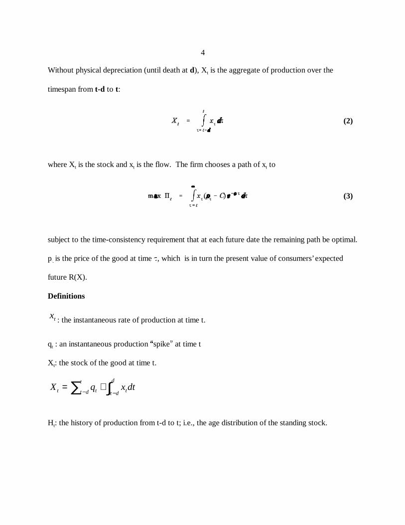
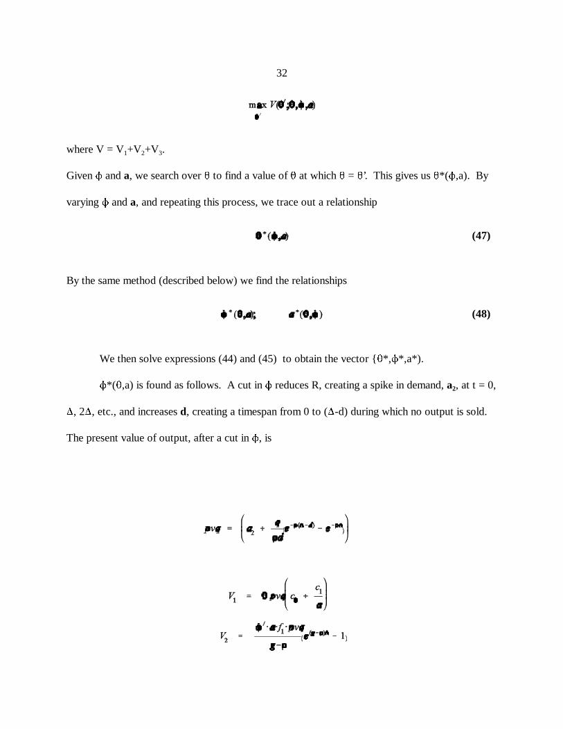
If the sale is to be repeated every d years, this increases the number of nonresidual

demanders who will retime their replacement so as to get onto the sale cycle. In other words, the

firm, by offering a sale, is opening a can of expectational worms. The spot profitability of a sale

must be weighed against the effect of such a sale on expectations.

In the model which we solve in the next section, we check for the profitability of a once-

only sale, assuming the sale itself has no effect on subsequent expectations. We find that a sale of

up to 20% increases spot profit by approximately 1%; any deeper sale reduces profit. We find

that no sale, predictably repeated every d periods, is profitable.

II. Solving the Maintenance Model

We seek an inherited vector, {2,N,a}, from which no permanent deviation in any

parameter is profitable. First, for a given {N,a} vector we seek a time-consistent 2 as follows:

Given a vector {2,N,a}, assume {N,a} remain fixed but 2 is cut to 2’. Such a cut reduces both R

and d, resulting in the output flow depicted in Figure 3. 2 is reduced at time 0; stock which

otherwise would have been retired at age d is now retired at age ). The size of this early-

retirement (and therefore replacement at time 0) stock is a . It generates a production spike at t =1

0, ), 2), etc., of magnitude a . There is another production spike, on the same time interval,1

resulting from the reduction in R. Call this spike a . The present value of future output, pvq, is2

given by

where

m m

31

where R’ = R(2’,N,a). Now define

is the profit, from time 0 forward, from selling the original equipment. Profit from aftermarket

sales on this original equipment, V , is 2

The remaining element of profit, V , is the aftermarket profit from the base already installed at3

time 0, but not yet retired:

where * is the age (ranging from 0 to )) of the installed base at time 0. The firm’s problem is to

32

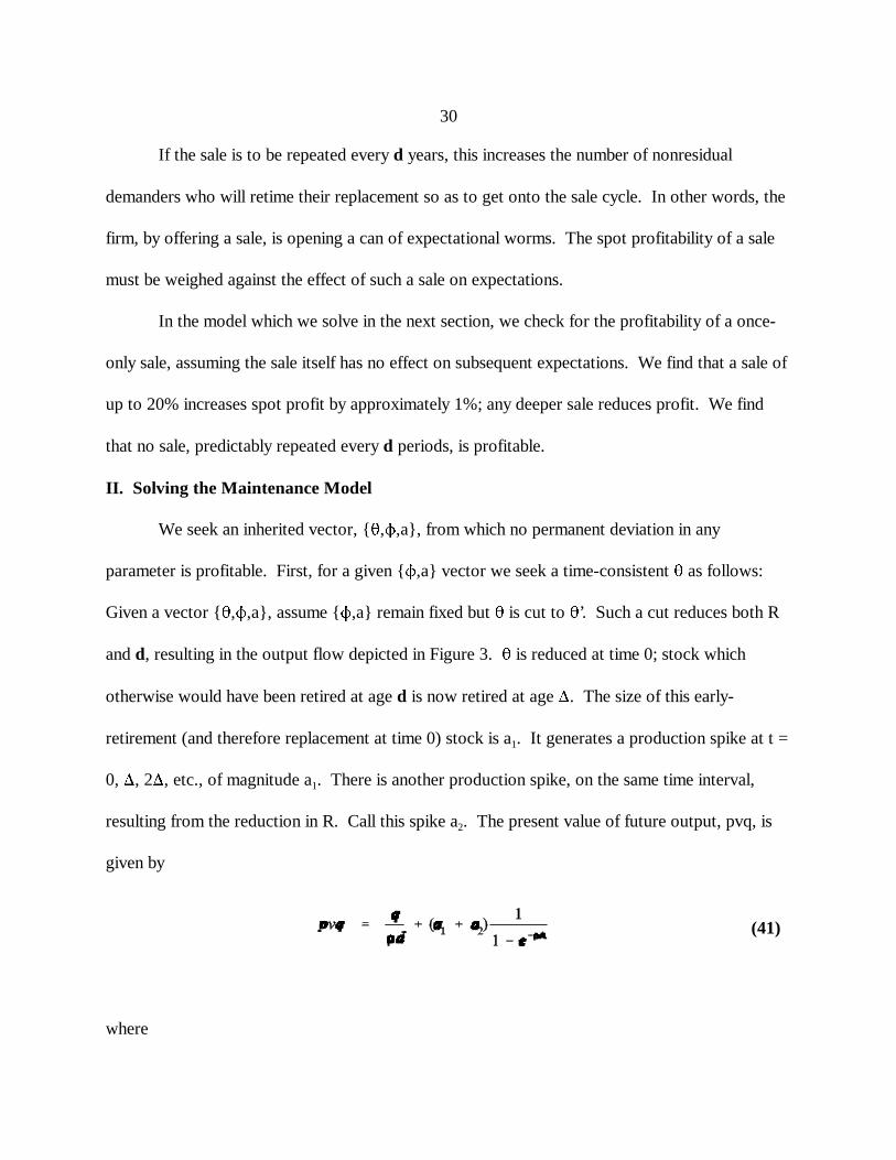
(47)

(48)

where V = V +V +V .1 2 3

Given N and a, we search over 2 to find a value of 2 at which 2 = 2’. This gives us 2*(N,a). By

varying N and a, and repeating this process, we trace out a relationship

By the same method (described below) we find the relationships

We then solve expressions (44) and (45) to obtain the vector {2*,N*,a*).

N*(2,a) is found as follows. A cut in N reduces R, creating a spike in demand, a , at t = 0,2

), 2), etc., and increases d, creating a timespan from 0 to ()-d) during which no output is sold.

The present value of output, after a cut in N, is

m m

m m

33

and

Holding 2 and a fixed we find the value of N such that N = N’ where N’ maximizes V.

Repeating over many values of 2 and a gives us the relationship N(2,a). By the same procedure

we find a’(2,N). First, define the pvq which flows after a rise in a (which reduces d and increases

R):

V and V take the same form as above. V , the present value of aftermarket profit from installed1 2 3

base, is given by

34

Using the same technique as above, we find a’(2,N). We now have a system of three

equations

Solving these equations through manual search, we are able to solve the system for the

vector {2’,N’,a’}, which is equal to the time-consistent PREE vector {2*,N*,a*}.

III. Why Didn’t Bond and Samuelson Find This?

Bond and Samuelson model the behavior of a Coase monopolist, whose good depreciates

at the exogenous rate *. They adopt the Stokey discrete-time formulation and expectations

function, equ. (5), and derive

B&S Proposition 1:

a. For any value of z (the trading period), the limiting stock falls with * (the less durability, the

more monopoly power);

b. For any value of *, the limiting stock falls with z (the longer the trading period, the greater the

ability to retain monopoly power);

c. For any value of *, the limiting stock approaches the competitive level as z 6 0 (as the trading

period approaches 0, then regardless of durability, monopoly power approaches 0).

In fact, even for goods with very modest durability (e.g., * = .8), B&S require a very long

trading period to sustain much monopoly power. Table A1 gives the ratio of B&S’s X& /X& , for *S R

= .2, * = .5, and * = .8 for trading periods of various lengths. (The competitive value of this ratio

35

With linear demand and constant marginal cost, deadweight loss is proportional to the15

square of the monopoly output restriction, so a 50% increase in output reduces deadweight lossby 75%.

is 2; the perfectly Coase-immune ratio is 1).

Table A1 B&S X /XS R

z and *

z *=.2 * = .5 * = .8

0.1 1.82 1.74 1.68

0.3 1.72 1.58 1.50

0.5 1.65 1.48 1.38

0.7 1.60 1.42 1.32

1 1.53 1.34 1.24

2 1.40 1.20 1.10

5 1.20 1.02 1.00

Even with 80% depreciation, at a one-year trading period X& is 24% greater than X& ; withS R

a trading period of 4 months, X& is 50% higher than X& . In other words, B&S tell us that theS R

Coase temptation is quite destructive of monopoly power, even for goods with virtually no

durability at all, so long as the trading period is not greater than about 6 months to a year. The

real message from Bond and Samuelson is not that the Coase temptation dissipates with imperfect

durability, but that even for goods with little durability, consumers receive much protection from

monopoly exploitation by the forces of Coase. Antitrust enforcement, it would seem, could be

limited to ensuring that trading periods remain shorter than 2 to 3 months.15

The question we address above is identical to that of Bond and Samuelson, and our

assumptions are identical except for the following:

(1) Our good is one-hoss-shay whereas theirs physically depreciates exponentially;

(2) Our time is continuous; their monopolist has commitment power for an exogenous period z

36

When time is literally continuous in B&S (z = 0), X& is not equal to the competitive16

level; it is indeterminate (see their equ. 11).

(for B&S continuous time is the special case where z = 0; as z 6 0 in B&S, the sales monopolist’s

behavior approaches competitive behavior, regardless of durability);

(3) They assume (without deriving it) a specific functional form for consumers’ expectations; we

infer our functional form as a consequence of consumers’ rationality.

Despite these apparently modest differences in modelling, our findings are almost

completely opposite to theirs.

Since B&S Propositions 1(a) and (b) above refer to finite trading periods, they have no

analog in our model. Their Proposition 1(c), however, suggests that as z 6 0 (as time approaches

continuous), monopoly output collapses to the competitive output, regardless of durability . Our16

conclusion, by contrast, is that with no trading period the durable-good monopolist’s price is

much greater than marginal cost, except for goods which last several decades.

The B&S results differ from ours only because of the difference in choice of G(@) function

and their discrete time assumption. As we have emphasized, this functional form for expectations

rests on no optimization decision. By contrast, we assume that consumers expect instant

saturation: G(@) = X& é X < X&,s,t, as dictated by consumers’ rationality.

G(X) = X& in Bond & Samuelson

Here we solve the B&S model, but replace discrete with continuous time and function

(5) with (6). Their modified model yields results essentially identical to our Part-I results.

The B&S first order condition for profit maximization (their equation (9)), is

j

m

m

37

(57)

where

are the values of the demand function parameters, integrated over the trading period z

and

Equilibrium requires that G(@) = X& é s,t,X < X&, and at X& any increase in X is regarded as

permanent, so G = 1. Substituting G = 1 into (57),3 3

j

38

(60)

(61)

The assumed expectations function is rational only if z = 0 (continuous time). As z 6 0, (60) 6

where $" and $$ are the demand function parameters for the instantaneous flow of service, and c$ is

the cost of producing the flow of service from the good. Using B&S’s expressions for X& and X& ,R C

(equs (5) and (7) in B&S) we can easily see that

Qualitatively and quantitatively, this is virtually identical to the analogous condition we derived in

(12), and an analogous proposition holds:

Modified B&S Proposition A1:

As * 6 0, X& 6 X&S C

As * 6 4, X& 6 X& .S R

Thus we see that the B&S structure, properly cast in continuous time with the only

expectations function consistent with continuous time, yields the same result as we found in Part

I: With no trading period, as durability approaches 0, the loss of monopoly power to Coase

39

approaches 0.

Quantitatively, this modified B&S formulation is also very similar to ours. Figure 3 plots

X& /X& as a function of 1/*, respectively for D = .05 and .10 (thus Figure 3 is the modified-B&SS R

analog to Figure 1). If we think of 1/* as approximately equal to d in the Part-I formulation, then

one can directly compare Figures 1 and 3. For 1/* = 10, X& /X& = 1.2 (again, for complete loss ofS R

monopoly power this ratio equals 2).

B&S’s finding that regardless of durability, sales-monopoly power goes to zero in

continuous time is an artifact of their expectations function; this function, in turn, is not consistent

with rationality in continuous time.

40

References

AMI v IBM 93-1586 3rd (1994).

Bond, Eric, and Larry Samuelson, "Durable Goods Monopolies with Rational Expectations andReplacement Sales," RAND Journal of Economics, Vol. 15 (1982), pp. 336-345.

Bulow, Jeremy, ""The Economic Theory of Planned Obsolescence," Quarterly Journal ofEconomics, Vol. 101 (1986), pp. 729-750.

Coase, Ronald, "Durability and Monopoly," Journal of Law and Economics Vol. 15 (1972), pp.143-149.

Crandall, Robert, Howard Gruenspecht and Lester Lave, Regulating the Automobile, Brookings,Washington, D. C. (1982).

Eastman Kodak Co v ITS, et al 112 S. Ct. 2072 (1992).

Rust, John, "When is it Optimal to Kill off the Market for Used Durable Goods," EconometricaVol. 54 (1986), pp. 65-86.

Schmalensee, Richard, "Market Structure, Durability, and Maintenance Effort," Review ofEconomic Studies, Vol. 41 (1974), pp. 277-287.

Stokey, Nancy, "Rational Expectations and Durable Goods Pricing," Bell Journal of Economics,Vol. 12 (1981), pp. 112-128.

Swan, Peter, "Optimum Durability, Second Hand Markets, and Planned Obsolescence," Journal ofPolitical Economy, Vol. 80 (1972), pp. 575-585.

Unites States v Aluminum Company of America, et al 148 F.2nd 416 (1945).