Some computational problems motivated by the Birch and Swinnerton-Dyer conjecture

SOME COMPUTATIONAL PROBLEMS MOTIVATED BY THE BIRCH AND

SWINNERTON-DYER CONJECTURE

by

Iftikhar A. Burhanuddin

A Dissertation Presented to theFACULTY OF THE GRADUATE SCHOOL

UNIVERSITY OF SOUTHERN CALIFORNIAIn Partial Fulfillment of theRequirements for the Degree

DOCTOR OF PHILOSOPHY(COMPUTER SCIENCE)

August 2007

Copyright 2007 Iftikhar A. Burhanuddin

Dedication

To Mom, Dad, Beauty and Dreams.

I need to live life

Like some people never will

So find me kindness

Find me beauty

Find me truth

When temptation brings me to my knees

And I lay here drained of strength

Show me kindness

Show me beauty

Show me truth

— ‘Learning to Live’ by Dream Theater

ii

Acknowledgements

At times our own light goes out and is rekindled by a spark from another person. Each

of us has cause to think with deep gratitude of those who have lighted the flame within

us. A. Schweitzer

I would like to thank Ming-Deh Huang for guiding my doctoral research, teaching me

about algorithms, cryptography and elliptic curves, listening patiently to my naıve ideas

and helping shape them into theorems, and most importantly giving me the freedom to

pursue the questions which captured my imagination.

It is a pleasure to thank William Stein for sharing his ideas and enthusiasm with

me, providing me opportunities and encouragement, treating me as a peer and being an

immense source of inspiration.

Special thanks to Sheldon Kamienny for always being enthusiastic about discussing

number theory and for his support, and to Thomas Geisser, Solomon Golomb, David

Kempe and Wayne Raskind for providing me with excellent career advice. Leonard

Adleman is an exemplar of how to be courageous in the pursuit of research, be it on

codewords of RSA or strands of DNA. I am grateful for his time and encouragement.

iii

Ashish Goel’s contagious fondness for theory left an impression on at least one budding

theoretician at USC and I appreciate his guidance. I would like to thank Charles Denis

Xavier for “remotely” sparking my interest in the theory of computation and enabling

me to posit “inspiration is an equivalence relation.”

Stimulating discussions with R. Balasubramanian, Henri Cohen, Brain Conrad, Luis

Dieulefait, Noam Elkies, Gerhard Frey, Marc Hindry, Kiran Kedlaya, David Joyner, David

Kohel, Kristin Lauter, Kapil Paranjape, Dinakar Ramakrishnan, Karl Rubin, Samir

Siksek, Joseph Silverman, Alice Silverberg, Kannan Soundararajan, Jon Voight, Felipe

Voloch, Mark Watkins, and Benjamin de Weger sparked new questions and directions of

research, and I express my gratitude to them.

I am especially thankful to S.S. Ranganathan, M.V. Tamhankar, and H. Subramanian

at BITS, Pilani and the teachers at Don Bosco, Madras for piquing my interest, as an

undergraduate student and a high-schooler, in mathematical structures of the discrete

kind.

I am extremely grateful to the organizers of workshops and conferences, who made

my travel to their events financially possible: Yves Aubry, Nils Bruin, Tanush Shaska and

the organizers of the Arizona Winter Schools and the SAGE workshops among others.

Each such trip introduced me to people who often sparked new questions to ponder, and

less often but no less importantly, provided the answers I was seeking.

I would like to thank Ming-Deh Huang, Gary Rosen and the Departments of Com-

puter Science and Mathematics for providing me with financial support during my years

at USC via NSF grants CCR-0306393 and CNS-0627458, and departmental graduate as-

sistantships. I would like to thank William Stein for creating SAGE and for providing

iv

me with access to the software systems PARI/GP, MAGMA, mwrank and SAGE via the

computers meccah.math.harvard.edu (funded in large part by William R. Hearst III)

and sage.math.washington.edu (funded by NSF Grant No. 0555776), without which

the computational aspects of this dissertation would not have seen the light of day. I am

lucky to have undertaken my doctoral studies in the City of Angels, where I had easy

access to the resources and faculties of Caltech, UCI, UCLA and UCSD, and I appreciate

their hospitality.

I am fortunate to have crossed paths the following wonderful people in Madras, Pilani,

Bangalore and Los Angeles: B.N. Anand, Arun Bruce, Amyn Dhala and Mario Sundar;

K.L.Arvind, Mitesh Agarwal, V.T. Bharadwaj, Sutanu Bhowmick, Naresh Chandran,

Saugata Chatterjee, Sandeep Dath, Prashant Gupta, Srivatsa Kedlaya, Ganesh Kumar,

Deepak Limaye, V.T. Mani, Prakash Math, Gaurav Mittal, Shailesh Murali, Prashant

Pandey, Kishore Patil, Shilpa Ranganathan, Rishi Sinha, Arvind Srinivasan and Srividya

Subramanian; Pradeep Abraham, Raju V. Kamal, T.S.R. Prasad and Raj Vallabhaneni;

Vanessa Carson, Frederic Chast, Karthik Dantu, Siva Jayaraman, Peter Molnar, Seema

Pai, Diana Popa, Deepak Ravichandran, Narayanan Sadagopan, Srikanth Saripalli and

Bilal Shaw; and certain pursuers of trivia around the world. Many thanks for the won-

derful memories.

Particular gratitude to my relatives for their love and encourgement. My parents

provided me with the best education that the circumstances afforded. I am indebted to

my dad, Dr. Kaleel Ahamath, for teaching me to dream, my mom, Parveen Kaleel, for

driving me to chase those dreams and my sister, Ambereen Burhanuddin, for the support

in realizing them. Thanks for believing in me.

v

I look forward to the exciting times ahead.

vi

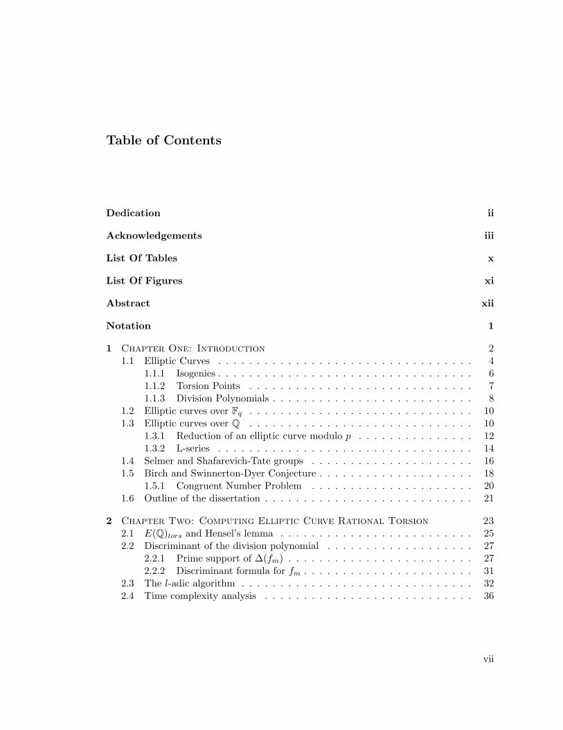
Table of Contents

Dedication ii

Acknowledgements iii

List Of Tables x

List Of Figures xi

Abstract xii

Notation 1

1 Chapter One: Introduction 21.1 Elliptic Curves . . . . . . . . . . . . . . . . . . . . . . . . . . . . . . . . . 4

1.1.1 Isogenies . . . . . . . . . . . . . . . . . . . . . . . . . . . . . . . . . 61.1.2 Torsion Points . . . . . . . . . . . . . . . . . . . . . . . . . . . . . 71.1.3 Division Polynomials . . . . . . . . . . . . . . . . . . . . . . . . . . 8

1.2 Elliptic curves over Fq . . . . . . . . . . . . . . . . . . . . . . . . . . . . . 101.3 Elliptic curves over Q . . . . . . . . . . . . . . . . . . . . . . . . . . . . . 10

1.3.1 Reduction of an elliptic curve modulo p . . . . . . . . . . . . . . . 121.3.2 L-series . . . . . . . . . . . . . . . . . . . . . . . . . . . . . . . . . 14

1.4 Selmer and Shafarevich-Tate groups . . . . . . . . . . . . . . . . . . . . . 161.5 Birch and Swinnerton-Dyer Conjecture . . . . . . . . . . . . . . . . . . . . 18

1.5.1 Congruent Number Problem . . . . . . . . . . . . . . . . . . . . . 201.6 Outline of the dissertation . . . . . . . . . . . . . . . . . . . . . . . . . . . 21

2 Chapter Two: Computing Elliptic Curve Rational Torsion 232.1 E(Q)tors and Hensel’s lemma . . . . . . . . . . . . . . . . . . . . . . . . . 252.2 Discriminant of the division polynomial . . . . . . . . . . . . . . . . . . . 27

2.2.1 Prime support of ∆(fm) . . . . . . . . . . . . . . . . . . . . . . . . 272.2.2 Discriminant formula for fm . . . . . . . . . . . . . . . . . . . . . . 31

2.3 The l-adic algorithm . . . . . . . . . . . . . . . . . . . . . . . . . . . . . . 322.4 Time complexity analysis . . . . . . . . . . . . . . . . . . . . . . . . . . . 36

vii

3 Chapter Three: Brauer-Siegel Analogue for Elliptic Curves 393.1 Brauer-Siegel Analogue . . . . . . . . . . . . . . . . . . . . . . . . . . . . 403.2 Conditional proof of the Brauer-Siegel Analogue . . . . . . . . . . . . . . 463.3 A natural question . . . . . . . . . . . . . . . . . . . . . . . . . . . . . . . 483.4 Big X’s . . . . . . . . . . . . . . . . . . . . . . . . . . . . . . . . . . . . . 49

4 Chapter Four: Notes on certain quartic twists of an elliptic curve 574.1 Analysis of ED . . . . . . . . . . . . . . . . . . . . . . . . . . . . . . . . . 59

4.1.1 Descent via two-isogeny . . . . . . . . . . . . . . . . . . . . . . . . 614.1.2 ED is conjecturally rank 1 . . . . . . . . . . . . . . . . . . . . . . . 63

4.2 The reduction . . . . . . . . . . . . . . . . . . . . . . . . . . . . . . . . . . 634.3 Heegner points computation . . . . . . . . . . . . . . . . . . . . . . . . . . 67

4.3.1 Indexes of Heegner points on ED . . . . . . . . . . . . . . . . . . . 684.3.2 A sketch of the time complexity analysis . . . . . . . . . . . . . . . 69

5 Chapter Five: Some thoughts on Parallel Computation 735.1 Torsion subgroup . . . . . . . . . . . . . . . . . . . . . . . . . . . . . . . . 76

5.1.1 A parallel algorithm . . . . . . . . . . . . . . . . . . . . . . . . . . 775.2 Tamagawa numbers . . . . . . . . . . . . . . . . . . . . . . . . . . . . . . 77

5.2.1 Tate’s algorithm . . . . . . . . . . . . . . . . . . . . . . . . . . . . 785.3 Periods . . . . . . . . . . . . . . . . . . . . . . . . . . . . . . . . . . . . . 785.4 Leading coefficient of LE(s) at s = 1 . . . . . . . . . . . . . . . . . . . . . 80

5.4.1 Root number . . . . . . . . . . . . . . . . . . . . . . . . . . . . . . 805.4.2 Fourier coefficients . . . . . . . . . . . . . . . . . . . . . . . . . . . 815.4.3 Order of the group E(Fp) . . . . . . . . . . . . . . . . . . . . . . . 82

5.5 Regulator . . . . . . . . . . . . . . . . . . . . . . . . . . . . . . . . . . . . 835.5.1 Determinant of a matrix . . . . . . . . . . . . . . . . . . . . . . . . 835.5.2 Canonical height of a point . . . . . . . . . . . . . . . . . . . . . . 83

5.6 Mordell-Weil group . . . . . . . . . . . . . . . . . . . . . . . . . . . . . . . 845.7 Size of the Shafarevich-Tate group . . . . . . . . . . . . . . . . . . . . . . 85

Bibliography 86

Appendix ADeciding whether #E(Qp)[p] is nontrivial . . . . . . . . . . . . . . . . . 91A.1 Computing #E0(Qp)[p] . . . . . . . . . . . . . . . . . . . . . . . . . . . . 92A.2 Algorithm when E has split multiplicative reduction at p . . . . . . . . . 97A.3 The complete algorithm . . . . . . . . . . . . . . . . . . . . . . . . . . . . 99

Appendix BDescent via 2-isogeny . . . . . . . . . . . . . . . . . . . . . . . . . . . . . . 101B.1 Structure of S(φ)(E) . . . . . . . . . . . . . . . . . . . . . . . . . . . . . . 101B.2 Structure of S(φ)(E′) . . . . . . . . . . . . . . . . . . . . . . . . . . . . . . 103B.3 An elliptic curve of conjectural rank 1 . . . . . . . . . . . . . . . . . . . . 105B.4 Generator of ED(Q) . . . . . . . . . . . . . . . . . . . . . . . . . . . . . . 107

viii

Appendix CBrauer-Siegel Ratio Graphs . . . . . . . . . . . . . . . . . . . . . . . . . . 109C.1 Ep : y2 = x3 + px . . . . . . . . . . . . . . . . . . . . . . . . . . . . . . . . 111C.2 Neumann-Setzer curves . . . . . . . . . . . . . . . . . . . . . . . . . . . . 114C.3 Cremona database . . . . . . . . . . . . . . . . . . . . . . . . . . . . . . . 117C.4 Stein-Watkins database . . . . . . . . . . . . . . . . . . . . . . . . . . . . 120

ix

List Of Tables

4.1 Invariants associated to the elliptic curves ED and EdKD . . . . . . . . . . 68

C.1 Distribution of #Xan(Ep) . . . . . . . . . . . . . . . . . . . . . . . . . . . 112

C.2 Smallest prime p such that #Xan(Ep) has a prescribed value . . . . . . . 112

C.3 Distribution of #Xan(E0) . . . . . . . . . . . . . . . . . . . . . . . . . . . 115

x

List Of Figures

C.1 BSR distribution for rank 0 elliptic curves Ep . . . . . . . . . . . . . . . . 113

C.2 BSR distribution for rank 0 Neumann-Setzer elliptic curves E0 . . . . . . 116

C.3 BSR distribution for rank 0 elliptic curves in the Cremona database . . . 118




C.7 BSR distribution for rank 0 elliptic curves in the Stein-Watkins database 121






xi

Abstract

This dissertation revolves around the BSD (Birch and Swinnerton-Dyer) conjecture for

elliptic curves defined over the rational numbers, a famous problem that has been open

for over forty years and one of the seven Millennium Prize problems. The BSD conjecture

is considered to be the first nontrivial number theoretic problem put forth as a result of

explicit machine computation — in the late ’50s at Cambridge University. The BSD

conjecture relates the rank of the Mordell-Weil group, the group of rational points of an

elliptic curve, a quantity which seems to be difficult to pin down, to the order of vanishing

of the L-function of the elliptic curve at its central point.

We make algorithmic and theoretical advances with regards to some of the terms ap-

pearing in the BSD formula, namely the sizes of the torsion subgroup and the Shafarevich-

Tate group.

Firstly, we introduce an algorithm to compute elliptic curve torsion subgroup. The

randomized version of this procedure runs in expected time which is essentially linear in

the number of bits required to write down the equation of the elliptic curve.

Next, we discuss a conjecture of Hindry, who proposed a Brauer-Siegel type formula for

elliptic curves. Driven by a suggestion of Hindry, we prove assuming standard conjectures

that there are infinitely many elliptic curves with Shafarevich-Tate group of size about

xii

as large as the square root of the minimal discriminant of the curve. This improves on a

result of de Weger.

Thirdly, we consider certain quartic twists of an elliptic curve. We establish a re-

duction between the problem of factoring integers of a certain form and the problem of

computing rational points on these twists. We illustrate that the size of Shafarevich-

Tate group of these curves will make it computationally expensive to factor integers by

computing rational points via the Heegner point method.

Finally, we sketch existing algorithms that compute the quantities appearing in the

BSD formula and introduce strategies to parallelize them.

xiii

Notation

The following standard notation will be used throughout this dissertation.

Z The integers.

Q The rational numbers.

Qp The p-adic numbers.

R The real numbers.

C The complex numbers.

H The upper half plane z ∈ C | im z > 0.

Z/nZ The ring of integers modulo n.

Fq The finite field with q elements.

R∗ The group of units in a commutative ring R with identity.

#S The cardinality of a set S.

char(R) The characteristic of a ring R.

f/R A polynomial f defined over a ring R, that is, the coefficients of f are in R.

1

Chapter 1

Chapter One: Introduction

At Kent he was curious about computer science but in just the introductory course Math

10 061 in Merrill Hall the math got to be too much for him. J. Updike in Rabbit is Rich

Astronomers and biologists have had telescopes and microscopes respectively to aid

in their research. With the advent of the computer, mathematicians acquired a powerful

tool, using which they could generate data, make conjectures and try turning them into

theorems — this was the dawn of the golden age of experimental mathematics.

This dissertation sits at the crossroads of number theory, algorithms and computation.

Our excursion into number theory had a cryptographic motivation, namely trying to

understand the Semaev-Smart-Satoh-Araki attack on the elliptic curve discrete logarithm

problem [Sem98]. This naturally lead to the question of deciding whether the p-part of a

certain group is nontrivial — see Appendix A. Proceeding from the above to computing

elliptic curve rational torsion and in turn to the BSD conjecture has been a wonderful

introduction to a world where conjectures abound and computations are indispensable.

2

The results which appear in this dissertation were obtained in collaboration with M.-D.

Huang.

A major area of research in number theory is the study of solutions in Q to a system

of polynomial equations defined over Q. For instance, rational solutions to the Fermat

equation xn + yn = 1, n > 2, which by a famous theorem of A. Wiles, do not exist.

The problem of deciding the existence and computation of such solutions even when

restricted to the one equation, two variable, degree 3 case becomes quite challenging and

hence interesting. Elliptic curves arise naturally in this context.

Questions about rational solutions can be transformed into questions about integer

solutions by switching to homogeneous coordinates, a process which “clears the denomi-

nators”.

Now suppose the homogeneous equation f(x1, . . . , xn) = 0 over Q has an integral

solution, then trivially it has a real solution and moreover f(X) ≡ 0 mod m for every

integer m.

One might wonder if the converse holds true. In the case of quadratic forms it is a

theorem (see [ST92, Page 15]).

Theorem 1.0.1 (Hasse) A homogeneous quadratic equation in several variables is solv-

able by integers, not all zero, if and only if it is solvable in R and Qp for each prime p.

The field of p-adic numbers Qp is the completion of Q with respect to the p-adic

absolute value. It can be viewed as a gadget which captures information about solutions

of an equation modulo powers of the prime p.

3

Proceeding to an equation of degree greater than 2, we see that the projective plane

curve over Q defined by the homogeneous equation 3x3+4y3+5z3 = 0 has a solution over

every completion of Q but no solution in Q. This is termed as the failure of the Hasse

local-global principle and it is this phenomenon which renders “local” methods unusable

and makes computing global points difficult in general.

The Birch and Swinnerton-Dyer conjecture can be viewed as an analogue of the Hasse

principle for elliptic curves as it gives us a formula for the size of the Shafarevich-Tate

group of an elliptic curve over Q, an object which measures the extent of the failure of the

global-local rule for the particular elliptic curve. But more importantly the conjecture

gives information about the rank of the elliptic curve, a fundamental algebraic invariant

via the order of zeros of the L-series of the elliptic curve, a complex analytic object.

Apart from the arithmetic problems which arise from the theory of elliptic curves,

what makes these objects interesting to computer scientists is that they can be used to

build cryptographic and coding theory systems [Kob94].

1.1 Elliptic Curves

It is possible to write endlessly on elliptic curve. (This is not a threat.) S. Lang [Lan78]

Our introductory definitions and theorems will closely follow J.H. Silverman’s exposi-

tion on elliptic curves [Sil92]. The eager reader should consult his book for background

material, proofs and further references.

4

Definition 1.1.1 An elliptic curve is a pair (E,O), where E is a curve of genus 1 and

O ∈ E. (We just write E for the elliptic curve, the point O being understood.) The elliptic

curve is defined over K, written E/K, if E is defined over K as a curve O ∈ E(K).

An elliptic curve over K is given by the Weierstrass equation

y2 + a1xy + a3y = x3 + a2x2 + a4x+ a6, (1.1)

where ai ∈ K. If characteristic of K is not 2 or 3 then E can be transformed to be of the

form

y2 = x3 + ax+ b,

where a, b ∈ K. The smoothness (or non-singularity) condition above is equivalent to

saying that the discriminant of E ∆(E) = −16(4a3 + 27b2) is nonzero. In projective

coordinates [x, y, z], the elliptic curve equation is given by

y2z = x3 + axz2 + bz3,

and the point O is taken to be the so-called point at infinity [0, 1, 0], the point of

intersection of the elliptic curve and z = 0, the line at infinity.

5

The chord-tangent construction Chord-tangent construction (namely P,Q,R ∈ E(K)

satisfy P +Q+ R = O if and only if they are collinear), can be used to turn E(K), the

set of K-rational points,

E(K) = (x0, y0) ∈ K ×K | y20 = x3

0 + ax0 + b ∪ O (1.2)

into an abelian group with the point O acting as the identity of the group. The fact that

makes elliptic curves friendly to computation is that the geometric construction turns out

to give a group law which is algebraic in nature [Sil92, Group Law Algorithm III.2.3].

1.1.1 Isogenies

After having presented the basic properties of the object, we now turn to the study

relationships of objects via maps between them. In particular, we are interested in maps

called morphisms which take O of one elliptic curve to that of another [Sil92, §III.3].

Definition 1.1.2 An isogeny between elliptic curves E1, E2 is a morphism

φ : E1 → E2

satisfying φ(O) = O. E1, E2 are said to be isogenous if there is a nontrivial isogeny

between them, that is an isogeny s.t. φ(E1) 6= O.

An important example of an isogeny is the multiplication by m morphism

[m] : E → E

6

defined as follows: [0]P = O, if m > 0 then [m]P = P + . . .+ P︸︷︷︸m times

, otherwise [m]P =

[−m](−P ). It is a fact that if m 6= 0, then [m] 6= [0]. Another important result is that

the kernel of a nonzero isogeny is a finite group.

If E is an elliptic curve over a field of characteristic zero, then the degree of φ, a

nonzero isogeny can be defined to be deg(φ) := # kerφ [Sil92, Theorem 4.10].

Theorem 1.1.1 Let φ : E1 → E2 be a non-constant isogeny of degree m. There exists a

unique isogeny

φ : E2 → E1

satisfying

φ φ = [m].

φ is called the dual isogeny to φ. If φ = [0], then we set φ = [0].

1.1.2 Torsion Points

The m-torsion subgroup of E, E[m] is defined to be ker([m]). The torsion subgroup of

E is the set of points of finite order, ∪∞m=1E[m]. If E is defined over K, then E(K)tors

denotes the points of finite order in E(K). The following fact gives us the structure of

the torsion subgroup.

Proposition 1.1.1 Let m ∈ Z,m 6= 0.

7

1. If char(K) = 0 or gcd(m, char(K)) = 1, then

E[m] ∼= (Z/mZ)2

2. If char(K) = p and m = pe, then either

E[m] ∼= O for all e = 1,2, . . . ; or

E[m] ∼= Z/mZ for all e = 1,2, . . . .

1.1.3 Division Polynomials

Division polynomials of an elliptic curve over a field K encode information about its

torsion points. We will restrict our attention to the case when K is a number field.

Moreover what we say will also hold for K being a finite field with char(K) > 3 when

the statements are viewed in the appropriate context. A general treatment of these

polynomials can be found in [BSS00, §III.4].

Let K be a number field and K be an algebraic closure of K. Let E be an elliptic

curve over K given by a Weierstrass equation y2 = x3 + ax+ b, where a, b ∈ R, where R

is the ring of integers of K.

8

We begin by presenting definitions and theorems concerning torsion points and poly-

nomials which characterize them. Define division polynomials Ψm recursively as follows:

Ψ1 = 1, Ψ2 = 2y, Ψ3 = 3x4 + 6ax2 + 12bx− a2,

Ψ4 = (2x6 + 10ax4 + 40bx3 − 10a2x2 − 8bax− 2a3 − 16b2)Ψ2,

Ψ2k+1 = Ψk+2Ψ3k −Ψk−1Ψ3

k+1, k ≥ 2

Ψ2k = (Ψk+2Ψ2k−1 −Ψk−2Ψ2

k+1)Ψk/Ψ2, k ≥ 2.

Define for m > 2, fm = Ψm, when m is odd and fm = Ψm/Ψ2, when m is even.

Observe that fm (also referred to as division polynomials) are univariate. Let d denote

deg fm, which is equal to m2−12 , if m is odd and m2−4

2 otherwise. The leading coefficient

of fm is m, when m is odd and m2 otherwise.

The x-coordinates of the m-torsion points of E correspond to the roots of fm in the

following way [BSS00, Corollary III.7]: Let P ∈ E(K), such that P is not a 2-torsion

point then P ∈ E(K)[m]⇔ fm(x(P )) = 0.

We will now define the discriminant of a polynomial and related notions [Coh93,

§3.3.2]. Let S be an integral domain with quotient field L and L be an algebraic closure

of L. Let g ∈ S[X] with n = deg(g), lc(g) be its leading coefficient and αi be the roots

of g in L. Define the discriminant of g to be

∆(g) = lc(g)n−1+deg(g′)∏

1≤i<j≤n

(αi − αj)2.

Let f = x3 + ax + b and hence ∆(f) = −(4a3 + 27b2). As indicated earlier, the

discriminant of the elliptic curve is defined to be ∆(E) = −16(4a3 + 27b2) and the letter

9

E is dropped when the curve is clear from the context. A formula for the discriminant

of the m-division polynomial of an elliptic curve can be found in §2.2.2.

1.2 Elliptic curves over Fq

Let E be an elliptic curve over Fq, the finite field with pn elements. H. Hasse proved the

following conjecture of E. Artin, which provides bounds on the size of E(Fq).

Theorem 1.2.1 (Hasse) Let E be an elliptic curve over Fq. Then

#E(Fq) = q + 1− aq, with |aq| ≤ 2√q

The Frobenius map Fq → Fq, x 7→ xq, induces an isogeny on E, which in turn induces

a map on the l-adic Tate module Tl(E), where l is a prime different from p. The aq

appearing in the above theorem is the trace of the Frobenius map acting on Tl(E) (see

sections III.7, V.2 of [Sil92] for details).

1.3 Elliptic curves over Q

The purpose of this section is to present some background material on elliptic curves over

Q before we introduce the BSD conjecture.

A theorem of L.J. Mordell states that E(Q) is finitely generated as a group. In other

words:

10

Theorem 1.3.1 (Mordell)

E(Q) ∼= E(Q)tors × Zr

where E(Q)tors, the torsion subgroup is finite and r is a non-negative integer called the

rank of E(Q).

Weil proved that the above theorem in the number field setting and the theorem is

known as the Mordell-Weil theorem and E(K) is called the Mordell-Weil group, where

K is a number field.

The free part of E(Q) is a mysterious entity as compared to the torsion subgroup.

Two important results about E(Q)tors are the following:

Theorem 1.3.2 (Nagell, Lutz) Let E be an elliptic curve over Q given by

y2 = x3 + ax+ b, a, b ∈ Z.

Suppose P ∈ E(Q)tors is a nontrivial point (P 6= O) then

1. x(P ), y(P ) ∈ Z and

2. either y(P ) = 0 or y(P )2|(4a3 + 27b2).

Theorem 1.3.3 (Mazur)

E(Q)tors∼=

Z/nZ, 1 ≤ n ≤ 10, 12, or

Z/2Z× Z/2nZ, 1 ≤ n ≤ 4.

11

Observe that an elliptic curve over Q can be transformed into the form which appears

in the Nagell-Lutz theorem using a change of coordinates [Sil92, Pages 46-50].

Let us assume that E is an elliptic curve over Q given by y2 = x3+ax+b, with a, b ∈ Z.

This implies that the division polynomials fm have integral coefficients and hence their

discriminants ∆(fm) ∈ Z, which is clear from the definition of the discriminant in terms

of the Sylvester matrix [Coh93, Lemma 3.3.4].

A global minimal model for an elliptic curve over Q is an integral Weierstrass equation

for which the absolute value of the discriminant is minimal among Weierstrass equations

with coefficients in Z for the elliptic curve. The discriminant of such a model is called

the (global) minimal discriminant. A closely related notion is that of a local minimal

model of an elliptic curve over Qp. This is a Weierstrass equation for the elliptic curve

with coefficients in Zp such that vp of the discriminant is minimal among all Weierstrass

equations with coefficients in Zp for the elliptic curve. (The valuation v at p of a rational

number r denoted by vp(r) is the largest integer power of p which divides the number.)

1.3.1 Reduction of an elliptic curve modulo p

For the sake of exposition let E be an elliptic curve over Q given by a global minimal

Weierstrass equation

y2 + a1xy + a3y = x3 + a2x2 + a4x+ a6.

with ai ∈ Z.

12

We can now talk about reducing this equation modulo a prime. Recall that an elliptic

curve is a smooth (or non-singular) curve, that is, there exists a unique tangent at each

point of the elliptic curve. Considering the above equation modulo a prime p, we obtain

an equation of a curve over Fp. If this reduced curve is non-singular (singular), then E

is said to have good (bad) reduction at p. The type of bad reduction is classified based

on the type of singularity (there is at most one), depending on whether the singularity is

a cusp or a node. The former reduction is termed additive and the latter multiplicative

reduction. If E has multiplicative reduction, then the reduction is said to be split (non-

split) if the slopes of the two tangents lines at the singular point are in (respectively not

in) Fp.

Let y2 = x3 + ax + b be a minimal Weierstrass equation of E an elliptic curve over

Qp, where a prime p > 3 then E is said to have good (bad) reduction at p if vp(∆) = 0

(vp(∆) > 0). On the other hand, the type of bad reduction — multiplicative or additive

— can be determined as follows: E has multiplicative reduction if and only if vp(∆) ≥ 1

and vp(ab) = 0 and it has additive reduction if and only if vp(a), vp(b) ≥ 1 [Sil92, Exercise

VII.7.1(b)]. Also E has split multiplicative reduction if and only if the reduction of −2ab

modulo p is a square [Milb, Page 27]. Otherwise E is said to have non-split multiplicative

reduction.

In general, to compute a minimal Weierstrass equation of an elliptic curve at p and

other local information, algorithm of J. Tate [Sil94, Chapter IV.9], [Cre97, §3.2] can be

used.

13

1.3.2 L-series

When faced with an interesting subset of the natural numbers, it is natural to encode

these numbers into a polynomial or power series and study its generating function. The L-

series of an elliptic curve is one such example. It captures information about the reduced

curve modulo each prime. An introduction to the content of this subsection can be found

in [Kna92], [Milb] and [Sil92, Appendix §16].

Let E be an elliptic curve over Q, p be a prime at which E has good reduction and

let Ep denote the elliptic curve modulo p. The zeta function of Ep over Fp is given by

Z(Ep/Fp;T ) = exp(∞∑

n=1

#Ep(Fpn) · Tn

n).

We know that Z(Ep/Fp;T ) is a rational function [Sil92, Theorem V.2.4]

Z(Ep/Fp;T ) =Lp(T )

(1− T )(1− pT ),

where

Lp(T ) = 1− apT + pT 2 ∈ Z[T ] and ap = p+ 1−#Ep(Fp).

14

The definition of Lp(T ) when E has bad reduction at p is as follows

Lp(T ) =

1− T if E has split multiplicative reduction at p

1 + T if E has non-split multiplicative reduction at p

1 if E has additive reduction at p.

Then in all cases we have the relation

Lp(p−1) =#Ens(Fp)

p,

where #Ens(Fp) is the group of non-singular Fp-points on E.

Definition 1.3.1 The L-series of E over Q is defined by the Euler product

LE(s) =∏p

Lp(p−s)−1.

The L-series of E an elliptic curve over Q is a priori defined only for complex numbers

s ∈ C with Re(s) > 32 .

Define ΛE(s) = (2π)−s · Γ(s) ·N(E)s/2 · LE(s), where Γ(s) is the Γ-function.

Theorem 1.3.4 (Hecke, Wiles et al.) The function ΛE(s) can be analytically contin-

ued to a complex analytic function on the whole of C, and it satisfies a functional equation

ΛE(2− s) = w(E) · ΛE(s), w(E) = ±1. (1.3)

15

Wiles et al. proved the modularity conjecture (now theorem) that essentially states

that LE(s) is the L-series associated to a modular form [BCDT01], and Hecke proved that

the L-series of a modular form analytically continues and satisfies the above functional

equation Eq. 1.3 (see [Milb, Theorem 26.5]). The import of Theorem 1.3.4 with regards

to the BSD conjecture is that LE(s) has a Taylor expansion at s = 1.

The integer N(E) is called the conductor of E, and the sign of the functional equation

w(E) is called the root number of E. The primes which divide N(E) are the same as the

primes which divide ∆(E) the minimal discriminant of E. For primes p ≥ 5,

vp(N(E)) =

0 if E has good reduction at p

1 if E has multiplicative reduction at p

2 if E has additive reduction at p.

Tate’s algorithm can be used to compute N(E), and there are formulae which can be

used to compute w(E) (see [Riz03]).

1.4 Selmer and Shafarevich-Tate groups

Let φ : E → E′ be an isogeny between elliptic curves E,E′ defined over Q and φ : E′ → E

be the dual isogeny of φ. The following exact sequence arises from the Galois cohomology

associated to E:

0→ E′(Q)/φ(E(Q))→ S(φ)(E)→X(E)[φ]→ 0 (1.4)

16

where S(φ)(E) is the φ-Selmer group of E over Q and X(E) is the (conjecturally finite)

Shafarevich-Tate group of E over Q. It is known that if #X(E) <∞ then it is a square

due to the existence of the Cassels-Tate pairing. We will proceed to give only a flavor of

these groups, their definitions can be found in [Sil92, Chapter X].

The elements of X(E) can be viewed as smooth curves called (principal) homogeneous

spaces with the property that they have a point over R and Qp for every prime p. An

element of X(E) which has a Q-point corresponds to the trivial element of X(E).

The group S(φ)(E) is finite and computable and gives upper bounds for the size of

E′(Q)/φ(E(Q)), the so-called weak Mordell-Weil group. It follows from the theory of

height functions on elliptic curves that, once we have computed the weak Mordell-Weil

group, the Mordell-Weil group E(Q) can be recovered.

If an element c ∈ S(φ)(E) maps to 0 ∈X(E), then by the exactness of the sequence

Eq. 1.4, c arises from an element of E′(Q)/φ(E(Q)). Therefore, this descent by φ isogeny

procedure reduces the computation of weak Mordell-Weil group to the question of exis-

tence of a rational point on a finite number of homogeneous spaces and the calculation of

these points. The inability to decide whether a homogeneous space is a nontrivial element

of X(E)[φ] is what makes rank computation using this procedure difficult.

In this context, the BSD conjecture comes to the rescue by providing information

about the rank of the elliptic curve, via the order of zeros of the L-series of the curve.

We give an overview of this conjecture in the next section.

17

1.5 Birch and Swinnerton-Dyer Conjecture

This remarkable conjecture relates the behavior of a function L at a point where it is not

at present known to be defined to the order of a group X which is not known to be finite!

J. Tate

B.J. Birch and H.P.F. Swinnerton-Dyer made their famous conjecture [BSD63] in-

spired by the class number formula and computational evidence obtained using the ED-

SAC2 computer at Cambridge during the late 1950s. This interplay of Computer Science

and Mathematics is what drew us to work on this conjecture. We fix some notation before

we present the BSD conjecture.

1. E : an elliptic curve over Q.

2. rE : is the algebraic rank of E, that is E(Q) = E(Q)tors × ZrE .

3. LE(s): the L-series of E.

4. L(t)E (1) := ( d

dsL(t)E (s))|s=1.

5. ranE := mint L

(t)E (1) 6= 0. That is the analytic rank of E is defined as order of

vanishing of LE(s) at s = 1.

6. ω := dx/(2y + a1x+ a3), the invariant differential on a global minimal Weierstrass

equation for E over Q, where a1, a3 are the coefficients of the Weierstrass equation

(Eq. 1.1).

7. Ω :=∫E(R) |ω| [Either the real period, or twice the real period, depending on whether

or not E(R) is connected.]

18

8. X(E): the Shafarevich-Tate group of E over Q.

9. Reg(E): the elliptic regulator of E(Q)/E(Q)tors, computed using the canonical

height pairing.

10. cp: #E(Qp)/E0(Qp), the Tamagawa number at prime p, where E0(Qp) is the sub-

group of the group of Qp-points of E that correspond to a non-singular point on

the reduced curve at p.

11. L∗E(1) := L(ran

E )

E (1)ranE ! , the leading coefficient of the Taylor expansion of LE(s) at s = 1.

Conjecture 1.5.1 (Birch, Swinnerton-Dyer)

ranE = rE (1.5)

L∗E(1) =#X(E) ·Reg(E) · Ω ·

∏p cp

(#E(Q)tors)2(1.6)

Eq. 1.5 is referred to as the Weak BSD conjecture.

The quote of Tate at the beginning of this section does not reflect the current state

of affairs with regards to the conjecture. The left hand side of Eq. 1.6 is well-defined (see

§1.3.2), and the Shafarevich-Tate group has been proved to be finite when the rank of the

elliptic curve is at most 1 by the work of B. Gross and D. Zagier, and V. Kolyvagin [Kol90].

Moreover,

ranE = 0⇒ rE = 0 (1.7)

ranE = 1⇒ rE = 1. (1.8)

19

There also results about the validity of the BSD formula in these cases — see [GJP+05].

1.5.1 Congruent Number Problem

The BSD conjecture is closely related to an ancient problem: find an algorithm to de-

termine whether or not a given integer n is the area of some right angled triangle all

of whose sides are rational numbers. If such a triangle exists, n is called a congruent

number. The following theorem of J.B. Tunnell states that assuming the BSD conjecture

there is a verifiable criterion for the congruent number problem [Kob93].

Theorem 1.5.1 (Tunnell) If n is a squarefree and odd (respectively, even) positive in-

teger and n is the area of a right angled triangle with rational sides, then

#x, y, z ∈ Z | n = 2x2 + y2 + 32z2 =12#x, y, z ∈ Z | n = 2x2 + y2 + 8z2

(respectively,

#x, y, z ∈ Z | n2

= 4x2 + y2 + 32z2 =12#x, y, z ∈ Z | n

2= 4x2 + y2 + 8z2).

If the weak BSD conjecture is true for the elliptic curves En : y2 = x3 − n2x, then,

conversely, these equalities imply that n is a congruent number.

20

1.6 Outline of the dissertation

An aspect which makes computing the mysterious invariants of the BSD conjectural

formula, namely the Shafarevich-Tate group and Regulator, interesting is that either

there are no known algorithms that exist or the ones that do exist take exponential time.

In chapter 2 we introduce an l-adic torsion computation algorithm for an elliptic

curve defined over Q. We begin the chapter by presenting the facts which we leverage

(Nagell-Lutz theorem and Mazur’s classification) and the techniques we utilize (Hensel

lifting) in the algorithm. The randomized version of this procedure runs in expected time

which is essentially linear in number of bits required to write down the equation of the

elliptic curve. We finish the chapter by analyzing the theoretical time complexity of the

algorithm.

In Chapter 3 we discuss a conjecture of Hindry, who proposed a Brauer-Siegel type

formula for elliptic curves over Q. Driven by a suggestion of Hindry, we prove assuming

standard conjectures that there are infinitely many elliptic curves with Shafarevich-Tate

group of size about as large as the square root of the minimal discriminant of the curve.

The next chapter is devoted to study of certain quartic twists of the elliptic curve

y2 = x3 − x, which raises interesting questions about integer factoring and heights of

rational points. We establish a reduction between the problem of factoring integers of a

certain form and the problem of computing rational points on these twists. We illustrate

that the size of Shafarevich-Tate group of these curves will make it computationally

expensive to factor integers by computing rational points via the Heegner point method.

21

Chapter 5 sketches existing algorithms that compute the invariants appearing in the

BSD formula and introduces strategies to parallelize them.

In Appendix A we devise a polynomial-time algorithm (polynomial in log p and the

bit length of the coefficients of the curve) that decides whether a given elliptic curve

over Qp has a nontrivial p-torsion part. The algorithm has two subroutines, the first

procedure computes #E0(Qp)[p] and the second determines #E(Qp)[p] when E has split

multiplicative reduction.

We present our original descent analysis for the aforementioned twists in Appendix B.

The proof suggested by an anonymous referee, which is found in §4.1.1, is much shorter

and perhaps more conceptual.

In Appendix C we tabulate computation driven by the questions and conjectures of

Chapter 3. Specifically, we compute the Brauer-Siegel ratio of E, for the elliptic curves

in databases [Cre], [SW02], and certain rank 0 elliptic curves.

I wrote this book and compiled in it everything that is necessary for the computer,

avoiding both boring verbosity and misleading brevity.

Ghiyath al-Din Jamshid Mas’ud al-Kashi in The Key to Arithmetic (1427)

22

Chapter 2

Chapter Two: Computing Elliptic Curve Rational

Torsion

The object of numerical computation is theoretical advance. A.O.L. Atkin [Bir98]

The Mordell-Weil theorem says that given an elliptic curve E over a number field K,

the group of K-rational points E(K) is finitely generated. This implies that the group

of K-rational torsion E(K)tors is finite. A theorem of B. Mazur states the groups which

can appear as E(K)tors, when K = Q.

Let E be an elliptic curve over Q defined by y2 = x3 + ax + b, where a, b ∈ Z and

let H(E) = max|a|3 , |b|2. Any elliptic curve over Q can be efficiently transformed to

the above form. The purpose of this chapter is to introduce methods which efficiently

compute elliptic curve rational torsion and to prove the following theorem.

Theorem 2.0.1 There is a randomized algorithm which computes E(Q)tors in O(logH(E))

expected time. The deterministic version of the algorithm runs in O(log2H(E)) time.

23

Notation. The soft-Oh notation O refers to the fact that logarithmic factors in the

length of input are ignored. A time step is a bit operation and the words size and bit

length of an integer will used synonymously. The discriminant of an elliptic curve E will

be denoted by ∆(E) or simply ∆.

We begin by briefly recalling the current approaches to determine E(Q)tors. Firstly,

one can compute torsion in a brute force fashion using the Nagell-Lutz theorem, which

states that torsion points are integral and bounded in magnitude, but this technique can

be computationally expensive. This naıve method was superseded by D. Doud’s complex

analytic cubic time algorithm [Dou98].

I. Garcıa-Selfa et al. [GSOT02] proposed a softly quadratic time algorithm (“softly”

refers to the soft-Oh notation), where they compute with the Tate Normal Form of an

elliptic curve. Their procedure uses R. Loos’ root-finding algorithm as a blackbox routine

and does not use any information about how the discriminants of Fm (polynomials which

arise in their algorithm) are related to the discriminant of the elliptic curve.

The roots of the so-called division polynomials correspond to the x-coordinates of

torsion points of the elliptic curve (see §1.1.3). Our algorithm discussed in §2.3 performs

root-finding on these polynomials using an l-adic approach. It has a worst case softly

quadratic running time and the randomized avatar of this method runs expectedly in

softly linear number of bit operations.

The basic idea of the algorithm is given an elliptic curve E over Q we view it as a curve

over Ql and use Hensel lifting to compute E(Ql)[m], the Ql-rational m-torsion points,

to desired precision. The values of m we investigate are dictated by Mazur’s result and

the sufficient precision to work with is supplied by the Nagell-Lutz theorem. We then

24

check to see if these points are in E(Q). We discuss time complexity analysis of the above

torsion computation procedure in §2.4.

The choice of the prime l rests on the fact that the prime support of the discriminant

of the m-division polynomial equals the prime support of m and the prime support of the

discriminant of the elliptic curve, which we prove in §2.2.1. This relationship between the

discriminants enables us to use a single “good” prime to compute the m-torsion for all

m. In order to relate ∆(fm), the discriminant of fm the m-division polynomial, to ∆, the

discriminant of the elliptic curve, we symbolically computed the discriminants of these

polynomials using for small values of m. This led us to discover a formula for ∆(fm). In

§2.2.2 we establish the equivalence of this formula when m is odd to a lemma of H.M.

Stark.

We would like to thank N.D. Elkies for pointing out that the running times of the

algorithms as presented in [BH05], being polynomials in log |∆(E)|, are conditional on

the weak version of the Frey-Szpiro conjecture (Conjecture 3.1.6). The mistake was due

to the assumption that length of input is asymptotically upper bounded by the size of

the discriminant logH(E) = O(log |∆(E)|). The same inaccuracy occurs in the paper of

Garcıa-Selfa et al [GSOT02].

2.1 E(Q)tors and Hensel’s lemma

The purpose of this section is to present some background material [Sil92, Chapter VIII]

before we introduce our elliptic curve rational torsion algorithm. A corollary of the

Mordell-Weil Theorem states that E(Q)tors is a finite group. To determine this group

25

the methods, which are currently in use, are guided by the theorems of Nagell-Lutz and

Mazur, which were stated in §1.3.

Suppose P ∈ E(Q)tors \E(Q)[2] then x(P ) will be a root of x3 + ax+ b− y(P )2. The

Nagell-Lutz theorem tells us that y(P )2|(4a3+27b2) which implies x(P )|(b−(4a3+27b2)/k)

for some k ∈ Z. If P ∈ E(Q)[2] and nontrivial then reasoning similar to the above leads

to x(P )|b since y(P ) = 0. Hence the coordinates of the torsion points are O(H(E)) in

magnitude.

The brute-force approach to compute torsion is to try out all the possible values for

y(P )2 such that it divides 4a3 +27b2. In the worst case this is computationally expensive

as it involves factoring and also 4a3 + 27b2 might have many square divisors giving rise

to many possibilities [Dou98].

Instead our algorithm performs root-finding on division polynomials using the follow-

ing variant of a lemma of K. Hensel [FGH00, Lemma 2.1]:

Lemma 2.1.1 (Hensel) Let u ∈ Zp and h ∈ Zp[x]. Let k be such that pk||h′(u) and

assume pn+k|h(u) for some n > k. Let

δ =p−kh(u)p−kh′(u)

and v = u− δ. Then v ≡ u mod pn, p2n|h(v) and pk||h′(v).

Hensel’s lemma states that an approximate root of a polynomial, which is not a

repated root, can be used to obtain a root which has at least twice as much precision. This

leads to a softly linear time method to find a root provided the initialization procedure,

26

where the approximate root is computed modulo pk, does not take more than softly linear

time.

2.2 Discriminant of the division polynomial

In this section we prove a few facts about the discriminant of fm, in particular Lemma

2.2.3, which makes l-adic torsion computation efficient.

2.2.1 Prime support of ∆(fm)

Lemma 2.2.1 Let m = 2k + 1 > 1 be an integer.

1. f ||f ′m

2. 22|f ′m

3. m|f ′m

4. md−1|∆(fm)

Proof 2.2.1 1. We will prove this by induction on m. f ′3 = 12f and the base case

holds. Suppose f |f ′i for all odd i < m. Let us assume k is odd (in the even case a

similar argument applies). We have Ψ2k+1 = f2k+1 = fk+2f3k − (fk−1Ψ2)(fk+1Ψ2)3

= fk+2f3k − fk−1f

3k+1Ψ

42 = fk+2f

3k − 24 · fk−1f

3k+1f

2. Now f ′2k+1 = f ′k+2f3k + 3 ·

fk+2f2kf

′k − 24 · (fk−1f

3k+1)

′f2 − 25 · fk−1f3k+1ff

′. f divides f ′k+2 and f ′k by the

inductive assumption and hence f divides each of the terms in f ′2k+1. In particular

f exactly divides f ′2k+1, otherwise f2k+1 would have repeated roots.

2. The argument is similar to the one above for part 1.

27

3. By [Cas49, Theorem 1 and Corollary 1] we have m|(Ψ2m)′ for any m and p - Ψ2

m

for any odd prime p. Suppose m =∏

i pi, where pi are odd primes. From the above,

m|ΨmΨ′m which implies pi|ΨmΨ′

m. Also pi - Ψm. Therefore pi|Ψ′m and therefore

m|Ψ′m.

4. The statement follows from part 3, lc(fm) = m and the matrix definition of the

discriminant, where the coefficients of f ′m are repeated on m2−12 rows.

Lemma 2.2.2 Let m = 2k > 2 be an integer.

1. k|∆(fm)

2. 22|f ′m

3. m|∆(fm)

Proof 2.2.2 1. Recall that lc(fm) = k and the coefficient of xd−1 in fm is 0. Consider

the matrix associated to R(fm, f′m). The first column of this matrix has k at entry

(1, 1) and km2−42 at (m2−4

2 , 1) and 0 elsewhere. The second column of this matrix

has k at entry (2, 2) and km2−42 at entry (m2−4

2 + 1, 2) and 0 elsewhere. Hence

k2|R(fm, f′m) and k|∆(fm) by the definition of discriminant.

2. 22|f ′4 and the base case holds. Suppose 22|f ′i for all even i < m. Now f ′2k =

(fk+2f2k−1 − fk−2f

2k+1)f

′k + (f ′k+2f

2k−1 + fk+2 · 2 · fk−1f

′k−1 − f ′k−2f

2k+1 − fk−2 · 2 ·

fk+1f′k+1)fk. Let us assume that k is odd (similar analysis for the even case).

From the previous lemma we know that 22 divides f ′k, f′k+2, f

′k−2. By the inductive

hypothesis 22 also divides f ′k−1, f′k+1. Hence 22|f ′m.

28

3. Follows from part 1 and 2.

Lemma 2.2.3 Prime support of ∆(fm) = prime support of m ∪ prime support of ∆,

where m > 2 is an integer.

Proof 2.2.3 Lemmas 2.2.1 and 2.2.2 state that 2 and m divide ∆(fm). Hence it suffices

to consider the primes p, which are relatively prime to m, and prove that p is in the prime

support of ∆(fm) if and only if p is in the set of primes where E has bad reduction over

Q.

Consider E to be an elliptic curve over Qp. We will take a minimal Weierstrass

equation denoted again by E and let its discriminant be ∆. Let L be a finite extension of

Qp. Let p = (π) be a prime over p in the ring of integers of L, Fp the residue field and e

the ramification index.

Let x = u2x′ + r, y = u3y′ + su2x′ + t be a change of coordinates giving a minimal

Weierstrass equation for E/L denoted by E′. The discriminant ∆′ for E′ satisfies ∆′ =

u−12∆ and hence vp(∆′) = −12vp(u) + vp(∆).

Let xi and x′i, 1 ≤ i ≤ d be the roots of the m-division polynomial associated to E and

E′ respectively. For i 6= j, we have vp(x′i − x′j) = vp(xi−ru2 −

xj−ru2 ) = vp(

xi−xj

u2 ) and hence

vp(xi − xj) = 2vp(u) + vp(x′i − x′j).

Now let us consider the valuation of the discriminant of the m-division polynomial

associated to E over Qp:

vp(∆(fm)) = (2d− 2)vp(lc(fm)) + 2∑

1≤i<j≤d

(2vp(u) + vp(x′i − x′j))

29

Suppose (m, p) = 1. Observe that vp(·) = evp(·). Since vp(m) = 0, we have vp(lc(fm)) =

vp(m) = 0 when m is odd and when m is even, we have vp(lc(fm)) = vp(m/2) = 0.

Case 1. Let E be an elliptic curve with potential good reduction over Qp. Let

L = Qp(E(Qp)[m]) be a finite extension of Qp over which E has good reduction [Sil94,

Proposition IV.10.3] which means vp(∆′) = 0 and therefore vp(u) = vp(∆)/12.

Moreover the reduction modulo p map E(L)[m]→ E(Fp)[m] is injective [Sil92, Propo-

sition VII.3.1 b] and hence vp(x′i − x′j) = 0 for all i 6= j and hence vp(∆(fm)) =

d(d− 1)/6 · vp(∆) which implies that

vp(∆(fm)) =d(d− 1)

6· vp(∆)

Hence if p is a prime of good reduction for E/Q then p - ∆(fm) and if p is a prime of

bad (additive) reduction then p|∆(fm).

Case 2. Let E be an elliptic curve with potential multiplicative reduction over Qp.

Let L ⊃ Qp(E(Qp)[m]) be a finite extension of Qp over which E has (split) multiplicative

reduction which means vp(∆′) > 0 and vp(c′4) = 0. We know that vp(c′4) = vp(u−4c4)

therefore vp(u) = vp(c4)/4. Also j = c34/∆ and this implies vp(c4) = 13 · (vp(∆) + vp(j)).

vp(∆(fm)) =d(d− 1)

6· (vp(∆) + vp(j)) +

∑1≤i<j≤d

2vp(x′i − x′j)

30

Now vp(∆) + vp(j) = 0 or > 0 depending on whether E has multiplicative or additive

reduction over Qp. Also in either case there exist i, j such that vp(x′i − x′j) > 0 (x-

coordinates of points which reduce to the singular point). Hence vp(∆(fm)) > 0 which

implies vp(∆(fm)) > 0.

Therefore if p is a prime of bad (additive or multiplicative) reduction for E over Q

then p|∆(fm).

2.2.2 Discriminant formula for fm

While investigating the discriminant of the m-division polynomials we stumbled upon a

precise formula which expresses ∆(fm) in terms of m and the discriminant of the elliptic

curve E. Based on symbolically computing the discriminants of m-division polynomials

for 3 ≤ m ≤ 12 using MAGMA [BCP97], we arrived at the following:

∆(fm) =

(−1)

m−12 · md−1 ·∆

d(d−1)6 m odd, or

24 · md−4 ·∆d(d−1)

6 m even.

(2.1)

The above formula in the odd case turns out to be equivalent to a lemma of H.M. Stark

[Sta82], which he proved using a complex-analytic approach, in particular L. Kronecker’s

second limit formula. Stark’s result deals with an elliptic curve E given in Weierstrass

normal form by y2 = 4x3 − g2x − g3, where g2 and g3 are rational. This equation can

be parameterized by the Weierstrass ℘-function, x = ℘(w), y = ℘′(w). Suppose N is odd

31

and let v1 and v2 run through a set of representatives of N−1Ω mod Ω, where Ω is the

period lattice of E. It is shown that

∏v1 6≡0,v2 6≡0,v1±v2 6≡0

[℘(v1)− ℘(v2)] = ±N−2(N2−3)∆(E)(N2−1)(N2−3)/6. (2.2)

Note that the above equation is a product over of differences of torsion points, which

are distinct and not inverses of each other.

Now we will establish the equivalence between our formula and that of Stark. Let

m be an odd number and let the roots of fm be denoted by xi, 1 ≤ i ≤ d, then by the

definition of the discriminant of a polynomial as stated in §1.1.3,

∆(fm) = lc(fm)2d−2∏

1≤i<j≤d

(xi − xj)2

where lc(fm) = m and d = deg fm = m2−12 . Using our formula modulo sign, we have

∏i6=j

(xi − xj) =∏

1≤i<j≤d

(xi − xj)2 =∆(fm)m2d−2

= m−m2−32 ∆

(m2−1)(m2−3)24 . (2.3)

The above equation is a product of differences of distinct x-coordinates of the torsion

points. Now comparing Eq. 2.2 with Eq. 2.3 and taking m = N we see that they are

equivalent up to fourth root, which is explained by the difference in the products.

2.3 The l-adic algorithm

Beware of bugs in the above code; I have only proved it correct, not tried it. D. E. Knuth

32

As stated in the introduction of this chapter, our algorithm works as follows: given

an elliptic curve E over Q we view it as a curve over Ql and using the appropriate factor

of the m-division polynomial we compute the Ql-rational m-torsion points to desired

precision and then check to see if they are, in fact, in E(Q). The prime l is chosen such

that E over Ql has good reduction. The integers m we have to consider are dictated by

Mazur’s theorem.

Algorithm 2.3.1 Input. An elliptic curve E in the form y2 = x3 +ax+ b, with a, b ∈ Z.

Output. < T, t >i, where T ∈ E(Q)[t] and i = 1, 2 and these points are the generators

of E(Q)tors.

1. Pick a prime l > 7 such that l - ∆.

2. Compute E(Ql)[2] using f .

3. r ← #E(Q)[2]− 1. Let R1, . . . , Rr be the nontrivial 2-torsion points.

4. If r = 0 then

(a) For p = 3, 5, 7 do the following:

i. If p - #E(Fl) then goto start of the loop and iterate with next prime.

ii. Compute Q ∈ E(Ql)[p] \ O using fp.

iii. If Q 6∈ E(Q) then goto start of the loop and iterate with next prime.

iv. If p = 5, 7 then Return < Q, p >.

v. If 32|#E(Fl) then

• Compute S ∈ E(Ql)[9] \ E(Ql)[3] using f9. If S 6∈ E(Q) then Return

< Q, 3 > else Return < S, 9 >.

33

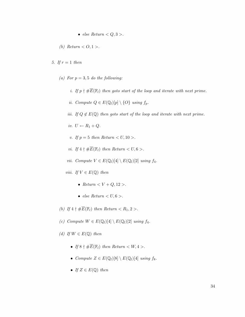
• else Return < Q, 3 >.

(b) Return < O, 1 >.

5. If r = 1 then

(a) For p = 3, 5 do the following:

i. If p - #E(Fl) then goto start of the loop and iterate with next prime.

ii. Compute Q ∈ E(Ql)[p] \ O using fp.

iii. If Q 6∈ E(Q) then goto start of the loop and iterate with next prime.

iv. U ← R1 +Q.

v. If p = 5 then Return < U, 10 >.

vi. If 4 - #E(Fl) then Return < U, 6 >.

vii. Compute V ∈ E(Ql)[4] \ E(Ql)[2] using f4.

viii. If V ∈ E(Q) then

• Return < V +Q, 12 >.

• else Return < U, 6 >.

(b) If 4 - #E(Fl) then Return < R1, 2 >.

(c) Compute W ∈ E(Ql)[4] \ E(Ql)[2] using f4.

(d) If W ∈ E(Q) then

• If 8 - #E(Fl) then Return < W, 4 >.

• Compute Z ∈ E(Ql)[8] \ E(Ql)[4] using f8.

• If Z ∈ E(Q) then

34

– Return < Z, 8 >.

– else Return < W, 4 >.

(e) Return < R1, 2 >.

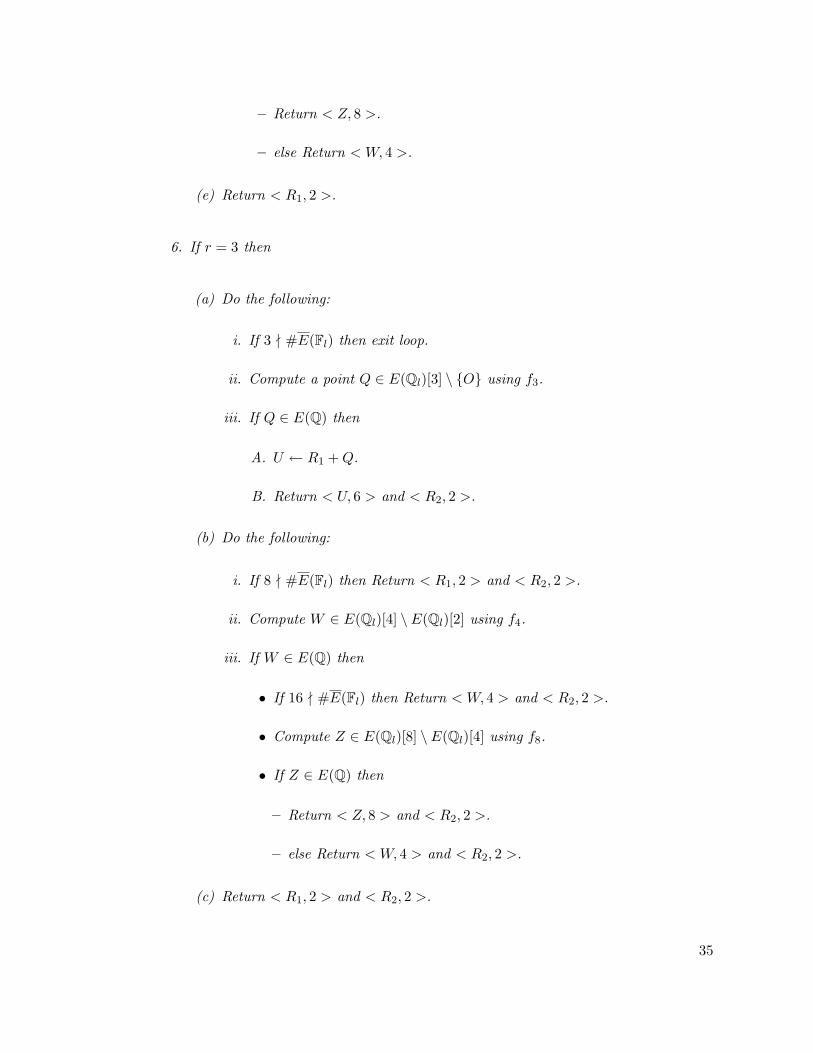
6. If r = 3 then

(a) Do the following:

i. If 3 - #E(Fl) then exit loop.

ii. Compute a point Q ∈ E(Ql)[3] \ O using f3.

iii. If Q ∈ E(Q) then

A. U ← R1 +Q.

B. Return < U, 6 > and < R2, 2 >.

(b) Do the following:

i. If 8 - #E(Fl) then Return < R1, 2 > and < R2, 2 >.

ii. Compute W ∈ E(Ql)[4] \ E(Ql)[2] using f4.

iii. If W ∈ E(Q) then

• If 16 - #E(Fl) then Return < W, 4 > and < R2, 2 >.

• Compute Z ∈ E(Ql)[8] \ E(Ql)[4] using f8.

• If Z ∈ E(Q) then

– Return < Z, 8 > and < R2, 2 >.

– else Return < W, 4 > and < R2, 2 >.

(c) Return < R1, 2 > and < R2, 2 >.

35

Theorem 2.3.1 The elliptic curve rational torsion algorithm works as desired.

Proof 2.3.1 We recall that the discriminant of a polynomial gives us an upper bound on

the precision at which the roots of the polynomial separate. The discriminant of the divi-

sion polynomial depends on the discriminant of the elliptic curve (Lemma 2.2.3, Eq. 2.1),

in particular we know that vl(∆(fm)) = (m2−3)(m2−1)24 vl(∆), where l is an odd prime such

that gcd(l,m) = 1 and m > 2.

Our choice of prime l > 7 and l - ∆ implies that E has good reduction at l and the

reduction map E(Ql)[m]→ E(Fl)[m] is injective for all values of m that we consider (m =

2, 3, 4, 5, 7, 8, 9). If m|#E(Fl) then the roots of fm are distinct modulo l and therefore we

can lift an Fl-root of fm to Ql using Hensel’s lemma with k = 0.

We note that x-coordinates of torsion points which are negative integers have l − 1

as a recurring digit in their l-adic expansion. Such integers can be recovered using the

following identity:∑O(dlogl H(E)e)

i=0 aili = −(l − a0 +

∑O(dlogl H(E)e)i=1 (l − 1 − ai)li), where

the left hand side represents truncated l-adic expansion of the negative integer. In other

words, as the final step of the algorithm we need to check whether a candidate x-coordinate

or its “negation” leads to a point in E(Q). This can be determined using the given integral

model of the elliptic curve.

2.4 Time complexity analysis

Let M(N) denote the bit operations required to multiply two numbers of size N . We

will assume that a fast integer multiplication algorithm like Schonhage-Strassen is used in

which case M(N) = O(N logN log logN) = O(N) [vzGG03, Theorem 8.24]. An integer

36

of size N can be expressed p-adically using a recursive procedure called radix conversion

in O(M(N log p) logN) time [vzGG03, Theorem 9.17]. Due to the quadratic convergence

of Hensel lifting, if the desired precision is N then we can perform lifting in O(M(N log p))

bit operations (assuming the degree of the polynomial is constant) [vzGG03, Theorem

9.26].

Given an elliptic curve with integral coefficients and discriminant ∆, we use Tate’s

algorithm [Cre97, Chapter 3.2] to compute the minimal Weierstrass equation at a prime p.

Let γ = maxH(E), p. Then the time complexity of Tate’s algorithm is O(log γ) (plus

the time to compute the number of roots of certain quadratic and cubic congruences

modulo p). The prime we work with is very small in bit length compared to log |∆|

(see below for details). Hence in our context the running time of Tate’s procedure is

O(logH(E)).

To find a prime l > 7 which does not divide ∆ deterministically takes O(log2 |∆|)

time [GSOT02], whereas resorting to a randomized algorithm takes O(logH(E)) ex-

pected time [vzGG03, Corollary 18.12 (ii)]. Since in both the determinstic and ran-

domized cases the magnitude of the prime selected is small — O(log |∆|) — the time

to compute #E(Fl) or to find a Fl-root of the division polynomial is negligible. Once

we find an approximate root of a division polynomial, we use Hensel lifting to com-

pute a Ql-root up to O(loglH(E)) accuracy and the time complexity of this operation is

O(M((loglH(E)) log l)) = O(logH(E)) bit operations.

Therefore, the routine to find the good prime dictates the overall running time of the

l-adic algorithm, which is O(log2 |∆|) deterministic time or an expected running time of

37

O(log |∆|). Phrasing the time complexity in terms of O(logH(E)), the length of input

of the algorithm, completes the proof of Theorem 2.0.1.

In practice to compute an upper bound for the size of the elliptic curve rational

torsion subgroup, #E(Fl) is computed for a few primes l of good reduction and their gcd

is determined. Moreover, this bound is a multiple of E(Q)tors and hence restricts the

orders of the torsion points which can exist for E. This recipe gives rise to the following

theoretical question: what is a bound for when the sequence

gcd(#E(Fl) | l is a odd prime of good reductionl≤X)X

stabilizes?

We plan to work on the above based on an idea of F. Voloch. This question becomes

quite interesting in the context of computing torsion for elliptic curves over number

fields, where structural results a la Mazur exist only for extensions of degrees at most

4 [KM95,JKP06] and the uniform bounds of J. Oesterle and P. Parent [Par99] are too big

to be useful to explicitly bound elliptic curve torsion over number fields of higher degrees.

In addition, we could elicit information about the existence of isogenous curves in certain

cases due to the results of J.-P. Serre and N.M. Katz [Kat81, Theorem 2].

38

Chapter 3

Chapter Three: Brauer-Siegel Analogue for Elliptic

Curves

Mathematics often owes more to those who ask questions than to those who answer

them. R. K. Guy [Guy04]

M. Hindry proposed a Brauer-Siegel type conjecture for abelian varieties over number

fields [Hin]. We raise questions and present results motivated by this conjecture special-

ized to elliptic curves over rationals. Appendix C tabulates computation inspired by the

contents of this chapter.

We begin by introducing the classical Brauer-Siegel theorem, which describes the

growth of the class number and regulator with respect to the discriminant of a number

field (see [Bra47] and [Coh93]).

Theorem 3.0.1 (Brauer, Siegel) Let K vary over a family of number fields of fixed

degree over Q. Then, as |d(K)| → ∞, we have

log(h(K) ·R(K)) ∼ log√|d(K)| , (3.1)

39

where h(K), R(K) and d(K) are the class number, regulator and discriminant of the

number field K respectively.

R. Brauer proved the above theorem by bounding left hand side (the residue of the

Dedekind zeta function of k at s = 1) of the class number formula. It is a natural to ask

whether an estimate similar to Eq. 3.1 holds in the context of elliptic curves.

3.1 Brauer-Siegel Analogue

We begin by defining notation, which will be used in this chapter.

Notation

• Let f(x) and g(x) be real-valued functions over R and let c ∈ R.

“f(x) ∼ g(x)” denotes that g(x) 6= 0 for sufficiently large x and limx→∞f(x)g(x) = 1.

Statements of the form “for every ε > 0, f(x) g(x)c+ε” should be interpreted

as “for every ε > 0, there exists a constant κ(ε) > 0 such that |f(x)| ≤ κ(ε) ·

g(x)c+ε, where κ(ε) depends on ε, and the inequality holds for all sufficiently large

values of x.” In the literature, “f(x) g(x)c+ε,” “f(x) ε g(x)c+ε” and “f(x) =

O(g(x)c+ε)” are used synonymously.

The notation has a definition analogous to .

• Every elliptic curve E is defined over Q, N(E) denotes its conductor, ∆(E) denotes

the global minimal discriminant of E, unless otherwise specified. The naıve height

of an elliptic curve E is defined to be h∗(E) = 112 ·log max|c4(E)|3 , |c6(E)|2, where

40

c4 and c6 are quantities associated to a global minimal Weierstrass equation for E.

The definitions of c4 and c6 can be found in [Sil92, §3.1], [Cre97, §3.1].

• Statements such as “for every ε > 0, f(E) g(E)c+ε,” where f(E) and g(E)

are real-valued invariants associated to elliptic curves E and c ∈ R, should be

interpreted as “for every ε > 0, there exists a constant κ(ε) > 0 such that |f(E)| ≤

k(ε) · g(E)c+ε, where κ(ε) depends on ε, and the inequality holds for all sufficiently

large values of h∗(E), where E ranges over Ei, a sequence of elliptic curves.” If

the sequence Ei is not specified it would imply that we consider all elliptic curves,

otherwise the sequence will be clear from the context.

The Shafarevich-Tate group and regulator of an elliptic curve are objects analogous

to the class group and regulator of a number field. Though the class number of a number

field — size of the class group — is finite, the size of the Shafarevich-Tate group of an

elliptic curve is only conjectured to be finite. This illustrates that analogous statements

between multiplicative groups and elliptic curves do not seem to carry over immediately.

S. Lang proposed a conjectural upper bound for the product of the size of the

Shafarevich-Tate group and the regulator of an elliptic curve. He arrived at this con-

jecture by bounding the quantities which appear in the the BSD formula [Lan83].

Conjecture 3.1.1 (Lang) For all elliptic curves E : y2 = x3 + ax+ b with a, b ∈ Z,

#X(E) ·Reg(E) H(E)112N(E)ε(N(E))crE (logN(E))rE (3.2)

41

where H(E) = max(|a|3, |b|2), rE is the Mordell-Weil rank of E, c is some universal

constant, and ε(N(E))→ 0 as N(E)→∞. In fact, ε(N(E)) may have the explicit form

ε(N(E)) = d(logN(E) · log logN(E))−12 ,

where d is some constant.

Hindry’s Brauer-Siegel type conjecture [Hin], which follows, implies that Lang’s bound

is “an equality in the limit”.

Conjecture 3.1.2 (Hindry)

log(#X(E) ·Reg(E)) ∼ h∗(E) (3.3)

In explicit terms, this conjecture asserts that

Conjecture 3.1.3 If Ei is a sequence of elliptic curves such that limi→∞ h∗(Ei) =∞.

then

limi→∞

log(#X(Ei) ·Reg(Ei))h∗(Ei)

= 1. (3.4)

The rank 0 version of Conjecture 3.1.3 reads

Conjecture 3.1.4 If Ei is a sequence of elliptic curves of Mordell-Weil rank 0 such

that limi→∞ h∗(Ei) =∞ then

limi→∞

log(#X(Ei))h∗(Ei)

= 1. (3.5)

42

We note the above conjectures and a lower bound for the regulator imply upper

bounds for the size of the Shafarevich-Tate groups of elliptic curves.

Conjecture 3.1.5 For every ε > 0, we have

#X(E) H∗(E)1+ε, (3.6)

where H∗(E) = exp(h∗(E)) = max|c4(E)|14 , |c6(E)|

16 .

The Frey-Szpiro conjecture (equivalent to the ABC conjecture [Ste]) states

Conjecture 3.1.6 (Frey, Szpiro) For every ε > 0, there exists cε > 0 such that

h∗(E) < (12

+ ε) logN(E) + cε. (3.7)

Combining Conjecture 3.1.5 with Conjecture 3.1.6 leads to

Conjecture 3.1.7 (Goldfeld, Szpiro) For every ε > 0, we have

#X(E) = O(N(E)12+ε). (3.8)

Of interest is a paper of D. Goldfeld and L. Szpiro [GS95], where they establish an

equivalence between Conjecture 3.1.7 and Conjecture 3.1.8.

Conjecture 3.1.8 (Szpiro) For every ε > 0, there exists κ(ε) > 0 such that

|∆(E)| < κ(ε) ·N(E)6+ε. (3.9)

43

The Frey-Szpiro conjecture implies the Szipro conjecture due to the identity 1728 ·

∆(E) = c4(E)3 − c6(E)2.

We proceed to present a result of B.M.M. de Weger [dW98], where conjectures in-

volving #X(E) are formulated, but first we state a conjecture which will be needed

(see [GS95]).

Conjecture 3.1.9 The Riemann hypothesis holds for the Ranking-Selberg zeta function

associated to the weight 32 modular form associated to an elliptic curve by the Shintani-

Shimura lift.

Lemma 3.1.1 (de Weger) For every ε > 0, there exist infinitely many elliptic curves

with

#X(E) |∆(E)|112−ε and (3.10)

#X(E) N(E)12−ε. (3.11)

Eq. 3.10 requires assuming the BSD conjectural formula in the rank 0 case. Eq. 3.11

requires assuming Szpiro’s conjecture (Conjecture 3.1.8) and Conjecture 3.1.9 in addition

to the BSD conjectural formula in the rank 0 case.

The proof of the lemma is constructive and produces a sequence of Frey-Hellegouarch

elliptic curves whose coefficients are related via theABC-conjecture and whose Shafarevich-

Tate groups are lower bounded as above.

Observe that Eq. 3.11 (together with Szpiro’s conjecture) would imply Eq. 3.10 but

de Weger’s proof requires merely assuming the BSD conjectural formula in the rank 0

44

case. Also Eq. 3.10 would imply Eq. 3.11 with the exponent 12 − ε replaced by 1

6 − ε, since

the Frey-Hellegouarch curves satisfy ∆(E) >> N(E)2.

In §3.4 we prove the main result of this chapter, which is a refinement of Lemma 3.1.1:

Lemma 3.1.2 For every ε > 0, there are infinitely many elliptic curves E such that

#X(E) |∆(E)|12−ε and (3.12)

#X(E) N(E)12−ε (3.13)

assuming that the BSD conjectural formula in the rank 0 case and Conjecture 3.1.9 are

true.

It suffices that the assumptions in these lemmas hold for the constructed sequence

of elliptic curves. Given the advances which have been made with regards to the BSD

conjecture in the rank 0 scenario, an interesting project would be to remove the BSD

formula assumption from the above lemma.

Comparing Lemmas 3.1.1 and 3.1.2, we see that the exponent in the lower bound in

terms of the discriminants is improved from 112−ε to 1

2−ε, but with the additional assump-

tion of Conjecture 3.1.9, and the lower bound in terms of the conductors is established

without assuming Szpiro’s Conjecture.

It is interesting to note that though the assumption of Conjecture 3.1.9 plays a crucial

role in the proof of Eq. 3.12, it does not play a role in the proof of Eq. 3.10. We wonder

if Eq. 3.12 could be established without this assumption.

Keeping in mind the lower bound satisfied by the Shafarevich-Tate groups of the

elliptic curves in Eq. 3.12 and the conjectural upper bound for Shafarevich-Tate groups

45

of elliptic curves (Eq. 3.8), it follows that the conductor of each of these elliptic curves

is “quite close” to its discriminant. This implies that the models of the aforementioned

elliptic curves are close to being global minimal models, a fact which is not apparent from

their construction.

We note that these conditional results involving #X(E) in the above discussion are

consistent with the Brauer-Siegel analogue conjectures introduced earlier.

3.2 Conditional proof of the Brauer-Siegel Analogue

The goal of this section is to present bounds (some of which are conjectural) for the

terms appearing in the BSD formula. Hindry proved that these bounds would imply a

Brauer-Siegel analogue for elliptic curves (Conjecture 3.1.2) and we sketch his proof in

this section. The contents of this section will also lay the foundation for proving results

in section 3.4.

Recall that the the BSD conjectural formula (Eq. 1.6) states that

#X(E) ·Reg(E) = L∗E(1) · #E(Q)2

Ω(E) ·∏

p cp(E), (3.14)

where L∗E(1) is the leading coefficient of the Taylor expansion of the L-series of E at

s = 1.

Mazur’s torsion classification theorem lists 15 groups which occur as the elliptic curve

torsion group and asserts that

1 ≤ #E(Q) ≤ 16. (3.15)

46

The Tamagawa number cp of an elliptic curve at a prime p lies in the following

interval [Sil92, Corollary 15.2.1]

cp ∈ [1,max4, logp(|∆(E)|)], (3.16)

and the product of cp over all the primes p is bounded as follows [dW98]

1 ≤∏p

cp |∆(E)|(m

log log|∆(E)| ) = O(∆(E)ε), (3.17)

where m is some constant [dW98, Theorem 3].

The real period of an elliptic curve E is bounded [Hin] as follows:

H(E) Ω(E)−1 H(E)1+ε (3.18)

where H(E) is the exponential of h(E), the height of E, a quantity which will not be

defined in this dissertation. For the purpose of analysis, h(E) can usually be replaced by

h∗(E), the naıve height of E, due to the following fact (see the discussion after Eq. 3.13

in [Hin])

Lemma 3.2.1 For any ε > 0, there exists κ(ε) such that

h(E) +O(1) ≤ h∗(E) ≤ (1 + ε) · h(E) + κ(ε). (3.19)

The leading coefficient L∗E(1) is conjecturally bounded as follows [Hin]. Hindry conjec-

tures that a lower bound similar to the one for the residue of the Dedekind zeta function

47

of a number field would also hold true for L∗E(1) (noting that “there is less evdidence”

for such a conjecture). On the other hand, it is claimed that the upper bound is implied

by assuming the generalized Riemann Hypothesis.

N(E)−ε |L∗E(1)| N(E)ε (3.20)

Combining the above bounds we have, for every ε > 0

(1− ε) · h∗(E) ≤ log(#X(E) ·Reg(E)) ≤ (1 + ε) · h∗(E) (3.21)

and this finishes Hindry’s conditional proof of Conjecture 3.1.2.

3.3 A natural question

A natural question motivated by the above conjectures — due to W. A. Stein — reads:

Are there infinitely many elliptic curves of Mordell-Weil rank 0 and trivial Shafarevich-

Tate group? More formally,

Question 3.3.1 Does there exist a sequence Ei of elliptic curves, such that

limi→∞

h∗(Ei) =∞, rEi = 0 and #X(Ei) = 1? (3.22)

Heuristics obtained by studying the Shafarevich-Tate group from the perspective of

Cohen-Lenstra type analysis for class groups [Del01] and from random matrix theory

(personal communication with M. Watkins) suggest that the set of rank 0 elliptic curves

48

with trivial Shafarevich-Tate group is a density 0 set. If the set is finite in size, then that

will be consistent with the above conjectures. On the other hand, if the set is infinite, then

that will imply that the Brauer-Siegel type conjectures do not hold due to the existence

of a counterexample to Conjecture 3.1.2.

In the context of multiplicative groups, the analogues of elliptic curves with rank

0 Mordell-Weil group and trivial Shafarevich-Tate group are imaginary quadratic fields

(as their unit groups are rank 0) with trivial class group. The analogue of Question

3.3.1 reads: Are there infinitely many imaginary quadratic fields with class number 1?

(Given n, the determination of the list of discriminants of imaginary quadratic fields

with n as their class number is called the Class Number problem.) It is a fact that

there are only finitely such fields Q(√d), where the discriminants d are from the list

−3,−4,−7,−8,−11,−19,−43,−67,−163 [Coh93, §5.3]. If such a phenomenon holds in

the elliptic curve scenario, there would exist only finitely many rank 0 elliptic curves

with trivial Shafarevich-Tate group. In other words, there would exist a bound such

that elliptic curves with discriminant greater than this bound would either have positive

Mordell-Weil rank or nontrivial Shafarevich-Tate group.

Suppose Question 3.3.1 is true, then this would imply that the conjectural bounds for

L∗E(1) are incorrect (Eq. 3.20).

3.4 Big X’s

At first glance one might expect the global minimal discriminant of an elliptic curve to

play the role of the discriminant of a number field in a Brauer-Siegel type formula for

49

elliptic curves. The following conjectural inequality, which states that the ratio of the

naıve height of an elliptic curve to its minimal discriminant is not a constant but varies

in a certain interval, lends support to the assertion that a Brauer-Siegel type statement

for elliptic curves as conjectured by Hindry (Conjecture 3.1.2) would not hold if the naıve

height is replaced by the logarithm of the discriminant or conductor of an elliptic curve.

112≤ h∗(E)

log |∆(E)|≤ 1

2+ ε. (3.23)

The first inequality follows from the definitions and the second inequality is a consequence

of the Frey-Szpiro conjecture. We would like to thank M. Hindry for bringing these

inequalities to our attention and for illustrating to us that the upper bound in Eq. 3.23

is met using a theorem of L.V. Danilov. We use this fact to prove Lemma 3.1.2.

A crucial ingredient in the proof of the lemma is Danilov’s paper [Dan82], where he

constructs infinitely many integers ak, bk such that as k →∞, |ak| , |bk| → ∞ and which

satisfy

∣∣a3k − b2k

∣∣ ∼ c |ak|12 , (3.24)

where c = 54√

5125 = 0.965 . . .. He uses these integers to prove the following theorem,

thereby confirming a conjecture of M. Hall (see [Dan82] for the details).

Theorem 3.4.1 (Danilov) For infinitely many integers x, y,

0 <∣∣x3 − y2

∣∣ < 0.97 |x|12 . (3.25)

50

As the pairs (ak, bk) satisfy Eq. 3.25, we have

|ak|3 ≤ max|ak|3 , |bk|2 < |ak|3 + 0.97 |ak|12 . (3.26)

Let us consider the sequence of elliptic curves Ek : y2 = x3 − 27ak − 54bk. The

discriminant and c-invariants of Ek are: ∆(Ek) = 26 · 39(a3k − b2k), and c4(Ek) = 64ak,

c6(Ek) = 66bk. We do not take (ak, bk) as the c-invariants of Ek, since it is not clear

if these pairs of integers satisfy Kraus’ conditions [Cre97, Proposition 3.1.1.], in other

words, whether there exist elliptic curves Ek with these c-invariants for all k.

Note that ∆(Ek) denotes the discriminant for the above model of Ek and not neces-

sarily the global minimal discriminant. It is not clear to us if (ak, bk) can be chosen such

that the discriminants are minimal.

By change of the variables, Eq. 3.26 reads

|c4(Ek)|3 ≤ max|c4(Ek)|3 , |c6(Ek)|2 < |c4(Ek)|3 + 0.97 · 610 |c4(Ek)|12 . (3.27)

The term |c4(Ek)|3 dominates over |c4(Ek)|12 for sufficiently large k, and hence

max|c4(Ek)|3 , |c6(Ek)|2 ∼ |c4(Ek)|3 , as k →∞. (3.28)

Utilizing Eq. 3.24 and the relations satisfied by ∆(Ek) and c4(Ek) in terms of ak, bk,

we get

c · 24 · 37 · |c4(Ek)|12 ∼ |∆(Ek)| , as k →∞. (3.29)

51

Combining Eq. 3.28 and Eq. 3.29 we have illustrated that as k →∞,

h∗(Ek) =112

log max|c4(Ek)|3 , |c6(Ek)|2 ∼12

log |∆(Ek)| . (3.30)

We record a lemma which is a consequence of this asymptotic growth of the naıve

height of elliptic curves Ek and the BSD conjectural formula.

Lemma 3.4.1 Assuming the BSD formula, the elliptic curve sequence Ek constructed

using Theorem 3.4.1 satisfies

log(#X(Ek) ·Reg(Ek)

L∗Ek(1)

) ≥ (12− m

log log |∆(Ek)|) · log |∆(Ek)| (3.31)

for sufficiently large k, where m is the constant used in bounding the product of the

Tamagawa numbers (Eq. 3.17).

The purpose of the remainder of this section is to use the aforementioned sequence of

elliptic curves Ek and construct another sequence E′k to prove the following lemma,

which would in turn imply Lemma 3.1.2.

Lemma 3.4.2 Let m be the constant used in bounding the product of the Tamagawa

numbers (Eq. 3.17). Assuming Conjecture 3.1.9, there exists a sequence of elliptic curves

E′k such that for sufficiently large k

h∗(E′k) <

12

log∣∣∆(E′

k)∣∣ (3.32)

h∗(E′k) ≥ (

12− m

log log∣∣∆(E′

k)∣∣) · log

∣∣∆(E′k)

∣∣ . (3.33)

52

In addition, assuming the rank 0 case of the BSD conjectural formula, we have

log #X(E′k) ≥ (

12− m


k)∣∣) · log

∣∣∆(E′k)

∣∣ (3.34)

for sufficiently large k.

The proof will be driven by techniques similar to the ones de Weger used in establishing

Lemma 3.1.1.

In what follows the elliptic curve Ek,q will denote the quadratic twist of Ek by q,

where q will depend on k and more precisely on the elliptic curve Ek (we do not use

subscripts to enhance readability). Twisting by q introduces a factor of a power of q to

the discriminant and the c-invariants, namely, ∆(Ek,q) = q6 ·∆(Ek), c4(Ek,q) = q2 ·c4(Ek)

and c6(Ek,q) = q3 · c6(Ek).

Multiplying the inequalities in Eq. 3.27 by q6 and switching to notation in terms of

Ek,q we get

|c4(Ek,q)|3 ≤ max|c4(Ek,q)|3 , |c6(Ek,q)|2 < |c4(Ek,q)|3 + 0.97 · 610q5 |c4(Ek,q)|12 . (3.35)

Let us start with Eq. 3.24 which (ak, bk) obey, namely for each δ > 0,

1− δ <a3

k − b2kc |ak|

12

< 1 + δ (3.36)

53

for sufficiently large k. Multiplying the numerator and denominator of the fraction by

q6, translating to notation in terms of Ek,q, taking sixth powers and retaining the same

notation for δ we get, for each δ > 0,

1− δ <|∆(Ek,q)|6

c′ · q30 |c4(Ek,q)|3< 1 + δ (3.37)

for sufficiently large k and where c′ = c6 · 224 · 342.

Assuming Conjecture 3.1.9 holds for each Ek, it is known that for every ε > 0, there

exists q < N(Ek)ε such that L(Ek,q, 1) 1 for sufficiently large k (consult [dW98] for

details). As L(Ek,q, 1) is bounded away from 0, Ek,q has Mordell-Weil rank 0 by the work

of V.A. Kolyvagin’s work on the BSD conjecture [Kol90].

Applying the inequality q < N(Ek)ε to the right of Eq. 3.35 we have, for every ε > 0,

max|c4(Ek,q)|3 , |c6(Ek,q)|2 < |c4(Ek,q)|3 + 0.97 · 610N(Ek)5ε |c4(Ek,q)|12 (3.38)

for sufficiently large k, and noting that 1 ≤ q for each elliptic curve, we have, for every

δ > 0,

1− δ <|∆(Ek,q)|6

c′ |c4(Ek,q)|3(3.39)


Combining Eq.3.40 and Eq. 3.39 proves that, for every ε > 0 and every δ > 0

max|c4(Ek,q)|3 , |c6(Ek,q)|2 <|∆(Ek,q)|6

c′(1− δ)+ 0.97 · 26 · 33N(Ek)5ε |∆(Ek,q)|

c(1− δ)(3.40)

54


Using the defintion of the naıve height of an elliptic curve, we have illustrated, for

each ε > 0 and every δ > 0,

h∗(Ek,q) <12

log |∆(Ek,q)| −112

log(c′(1− δ)) +112

log(1 + c′′N(Ek)5ε

|∆(Ek,q)|5) (3.41)

for sufficiently large k, where c′′ = 0.97 · 26 · 33. This proves Eq. 3.32.

On the other hand, applying the inequality q < N(Ek)ε to the inequality on the right

of Eq. 3.37 we have, for each ε > 0 and for each δ > 0,

|∆(Ek,q)|6

c′ ·N(Ek)30ε |c4(Ek,q)|3< 1 + δ (3.42)


The combination of the inequality on the left of Eq. 3.35 with Eq. 3.42 results in: for

each ε > 0 and for each δ > 0,

max|c4(Ek,q)|3 , |c6(Ek,q)|2 > c′−1 · |∆(Ek,q)|6 ·N(Ek)−30ε · (1 + δ)−1 (3.43)

for sufficiently large k. By the defintion of the naıve height of an elliptic curve and the

fact that |∆(Ek,q)| ≥ N(Ek), we obtain, for each ε > 0 and for each δ > 0,

h∗(Ek,q) > (12− 5ε

2) log |∆(Ek,q)| −

112

log(c′ · (1 + δ)) (3.44)

for sufficiently large k, where c′ = c6 · 224 · 342. This proves Eq. 3.33.

55

Denote by E′k the rank 0 quadratic twist of Ek by q such that L(Ek,q, 1) 1. Under

the BSD conjectural formula (rank 0 case), we have proved that

log #X(E′k) > (

12− 5ε

2− m


k)∣∣) · log

∣∣∆(E′k)

∣∣ (3.45)

for sufficiently large k, where m is the constant used in bounding the product of the

Tamagawa numbers (Eq. 3.17).

This finishes the proof of Lemmas 3.4.2 and 3.1.2. A question which arises in this

context is whether there exist sequences of elliptic curves which could be used, in lieu of

the one constructed using Danilov’s theorem, to prove the aforementioned lemmas and

perhaps yield easier proofs.

A final remark we would like to make is that analysis similar to above discussion can

applied to a sequence of elliptic curves Ei with c4(Ei) = 0 for all i (or c6(Ei) = 0). For

instance, the elliptic curves Ep in Appendix C.1 fit this description. Such elliptic curves

could be used to prove

h∗(E′i) ∼

112

log∣∣∆(E′

i)∣∣ , (3.46)

where E′i are rank 0 quadratic twists of Ei such that LE′

i(1) 1 for sufficiently large

values of i. This would imply that there are infinitely many elliptic curves E′ with

#X(E′)∣∣∆(E′)

∣∣ 112−ε ; (3.47)

a result on the lines of de Weger’s work — see Lemma 3.1.1.

56

Chapter 4

Chapter Four: Notes on certain quartic twists of an

elliptic curve

The problem of distinguishing prime numbers from composite numbers, and of resolving

the latter into their prime factors is known to be one of the most important and useful

in arithmetic. C. F. Gauss in article 329 of Disquisitiones Arithmeticae (1801).

In this chapter we investigate certain quartic twists of the elliptic curve y2 = x3 − x

and present some of their interesting properties. Specifically, we consider the family of

elliptic curves ED : y2 = x3 −Dx, where D = pq with p and q distinct prime numbers,

p ≡ q ≡ 3 mod 16. These elliptic curves have complex multiplication by Q(i). The

2-torsion point (0, 0) generates the torsion subgroup of the Mordell-Weil group ED(Q).

Employing the method of two-descent, we show that under the Birch and Swinnerton-

Dyer conjecture, the Mordell-Weil rank of ED is one.

Let E′D denote y2 = x3 + 4Dx the isogenous curve of ED, and C ′

d represent the

homogeneous spaces dW 2 = d2 −DZ4 of E′D.

57

We argue that any point R of the Mordell-Weil group ED(Q) which is not in 〈(0, 0)〉+

2ED(Q) must behave differently with respect to p-adic and q-adic valuations. This sets

the stage for reductions between the problem of factoring integers of the form D and the

problem of computing non-torsion rational points on ED.

In one direction, we prove that if there exists a rational point of the above form such

that its naıve height is polynomial in the naıve height of the elliptic curve h∗(ED), then

factoring D is polynomial time reducible to computing a non-torsion rational point of

ED.

In the other direction, we show that if either of the homogeneous spaces C ′p or C ′

−q of

E′D has a rational point whose naıve height is bounded by a polynomial in log h∗(ED), then

computing a non-torsion rational point of ED is polynomial time reducible to factoring

D.

The chapter ends with a discussion about Heegner point computation restricted to

these elliptic curves ED. We observe the dependence of the Heegner index on #X(ED).

Assuming that the Shafarevich-Tate groups tend to get “big” (for instance by the Brauer-

Siegel Analogue — Conjecture 3.1.2), it follows that factoring numbers of the form D by

computing a point in ED(Q) via the Heegner point method would be computationally

expensive.

58

4.1 Analysis of ED

In this section we will study a particular class of elliptic curves parameterized by primes p

and q and obtain the structure of their Mordell-Weil groups subject to congruence condi-

tions. The analysis in this section closely follows §X.6 from J.H. Silverman’s book, which

in turn exploits Proposition X.4.9 (Descent via Two-isogeny) from the same book [Sil92].

The reader eager to learn about the reduction mentioned in the chapter’s introduction

can skip this section.

Let ED over Q be the elliptic curve

ED : y2 = x3 −Dx.

where D ∈ Z (the subscript D will be dropped when it is clear from the context). Then

ED is isogenous to the elliptic curve

E′D : Y 2 = X3 + 4DX

via the isogeny φ : ED → E′D, (x, y) 7→ (y2/x2,−y(D + x2)/x2) and let φ : E′

D → ED be

the dual isogeny of φ.

We will consider the curves Epq : y2 = x3 − pqx, where p and q are odd and distinct

primes and perform descent via φ, which is an isogeny of degree 2.

Let MQ be the set of primes of Z and ∞ (that is, a complete set of inequivalent

absolute values on Q). Let S = ∞, 2, p, q ⊂ MQ and Qν denote the completion of Q

59

with respect to the absolute value associated to ν ∈ S. In particular, Q∞ denotes R and

for ν ∈ S \ ∞ and Qν denotes the ν-adic numbers. Let

Q(S, 2) := b ∈ Q∗/Q∗2 | ν(b) ≡ 0 mod 2 for all ν 6∈ S.

We take the following representatives for the cosets in Q(S, 2):

±1,±2,±p,±2p,±q,±2q,±pq,±2pq.

Let WC(E) denote the Weil-Chatelet group of E, the group of equivalence classes of

homogeneous spaces for E over Q. For each d ∈ Q(S, 2), the corresponding homogeneous

spaces Cd ∈ WC(E) and C ′d ∈ WC(E′), also referred to as quartics, are given by the

equations

Cd : dw2 = d2 + 4pqz4,

C ′d : dW 2 = d2 − pqZ4.

The φ-Selmer group can be viewed as a subset of Q(S, 2) as follows:

S(φ)(E) ∼= d ∈ Q(S, 2) : Cd(Qν) 6= ∅ for all ν ∈ S.

The φ-Selmer group S(φ)(E′) has an analogous isomorphism where Cd is replaced by C ′d.

60

The images of (0, 0), the 2-torsion point of E′(Q) and E(Q) in the Selmer groups are

given by

pq ∈ S(φ)(E) and − pq ∈ S(φ)(E′) (4.1)

respectively.

4.1.1 Descent via two-isogeny

We restrict our attention to elliptic curves

E = ED : y2 = x3 −Dx (4.2)

whereD = pq, p and q are distinct primes such that p ≡ q ≡ 3 mod 16 and (pq ) = (−q

p ) = 1.

In this subsection we perform descent on the 2-isogenous elliptic curves E and E′.

We would like to thank an anonymous referee for providing us with the following elegant

argument. Our original analysis can be found in Appendix B.

When K = Q or Qν , we have the exact sequence

0→ E′[φ]→ E′ → Ef→ K∗/K∗ 2, (4.3)

with f induced by P 7→ x(P ) for the models above. When K = Qν , we write S(φ)(K) for

the actual image of f . Let the group S(φ)(Q) be obtained by globalizing the local data.

It is identical to the Selmer group S(φ)(E′) introduced in §1.4.

61

Suppose P ∈ E(Qν), ν being equal to 2 or a place of good reduction then 2|ν(x(P ))

and we find that f(P ) ∈ Z∗ν .

For ν = p or ν = q, E has bad, type III reduction and [E : E0] = 2 [Sil92, Table

15.1]. The group E(Qν) is generated by E0(Qν) and the point T = (0, 0). Since both

E1(Qν) ∼= Zν and E0(Qν)/E1(Qν) ∼= Ens(Fν) ∼= Fv (the last ismorphism due to the type

of reduction being additive) are divisible by 2, so is the group E0(Qν). It follows that

S(φ)(Qν) = 〈−pq〉. We recall that it is assumed that p ≡ q ≡ 3 mod 16, labeled so that

(p/q) = (−q/p) = 1. Since p and −q are squares modulo q and modulo p respectively, we

have illustrated that S(φ)(Qp) = 〈p〉 and S(φ)(Qq) = 〈−q〉.

For d ∈ Q(S, 2) to be an element of S(φ)(Q), it must necessarily correspond to a unit

in S(φ)(Qv) when ν is 2 and when ν is a place of good reduction, and when ν is p and q,

d must map to an element of S(φ)(Qv). In this fashion based on local conditions, we can

eliminate the elements of Q(S, 2) which cannot occur as elements of S(φ)(Q). It follows

that the Selmer group is 〈p,−q〉.

Next, we consider the group S(φ)(Q). If P ∈ E′(R) then x(P ) ≥ 0. This fact coupled

with reasoning similar to the preceding paragraphs show that S(φ)(Q) = 〈pq〉.

When the rank of E(Q) is 1, it follows that the points on E(Q) map onto S(φ)(Q).

Therefore we find that for any point R in E(Q) but not in E[φ] + 2E(Q), νp(x(R)) and

νq(x(R)) have opposite parity.

62

4.1.2 ED is conjecturally rank 1

The purpose of this subsection is to conditionally prove that the elliptic curves ED have

Mordell-Weil rank 1. Driven by techniques used in proving Proposition X.6.2(c) [Sil92],

we obtain

rE + dim2 X(E′/Q)[φ] = dim2 S(φ)(E) + dim2 S

(φ)(E′)− 2

= 1.

where dim2 is the dimension as a Z/2Z-vector space. In particular, rE ≤ 1.

Next, we will investigate the zeros of the L-series of E at s = 1. For the curves of

interest the global root number w(E) can be computed from the formulae in [BS66] and

it equals -1. Evaluating the functional equation of ΛE(s) at s = 1 (Eq. 1.3), we have

ΛE(1) = −ΛE(1) and hence ΛE(1) = 0. This implies that LE(1) = 0, in other words,

ranE > 0.

If ranE = 1, that is, L(1)

E (1) 6= 0, then rE = 1, by a result of V.A. Kolyvagin [Kol90].

The lemma below records our result.

Lemma 4.1.1 Let E be an elliptic curve as defined in Eq. 4.2. Assuming ranE = 1 (or

alternatively the BSD conjecture), rE = 1.

4.2 The reduction

Definition 4.2.1 Let E be an elliptic curve over Q, P ∈ E(Q) and x(P ) = ab , we define

the naıve height of P to be hx(P ) = log max|a|, |b|.

63

Definition 4.2.2 Let E be an elliptic curve over Q and define the naıve height of the

elliptic curve to be

h∗(E) =112

log max|c4(E)|3 , |c6(E)|2

where c4(E) and c6(E) are the c-invariants associated to a minimal model of E.

Definition 4.2.3 Let f ∈ Z[X].

SEf := E/Q | there exists a non-torsion point T ∈ E(Q) with dhx(T )e ≤ f(h∗(E)).

In other words, SEf is the set of elliptic curves which have a non-torsion rational

point whose bit length is bounded by a polynomial f in the bit length of the respective

elliptic curve.

Let the problem of factoring integers of the form D (as defined in Eq. 4.2) be denoted

by IFD. Let the problem of computing a non-torsion rational point of ED be denoted by

CRPSED. We note that h∗(ED) = log(24 · 3 ·D) = O(logD).

Let us recapitulate the results of the previous section: ED has conjectural rank 1 and

the x-coordinate of a generator of ED(Q) has different valuations with respect to p and

q.

Definition 4.2.4 Let f ∈ Z[X]. SEDf := ED/Q | ED ∈ SEf.

The set SEDf being infinite in size, follows from conjectural evidence which is pre-

sented toward the end of this section — Remark 4.2.1.

64

Fixing f a polynomial with integral coefficients, let the problem of factoring integers

of the form D such that the associated elliptic curve ED ∈ SEDf be denoted by IF fD

and the problem of computing a non-torsion rational point of ED ∈ SEDf be denoted

by CRPSEfD. We are ready to prove the following result:

Theorem 4.2.1 Fixing f ∈ Z[X], IF fD ≤P CRPSEf

D.

Proof 4.2.1 Given f,D, a blackbox algorithm for CRPSEfD can be used to compute

P , a non-torsion rational point on ED. A point R ∈ ED(Q) \ (ED[φ] + 2ED(Q)) can be

constructed by “halving” P using the duplication formula [Sil92, Algorithm 2.3 (d)]. Since

vp(x(R)) 6= vq(x(R)), p and q can be recovered. Moreover, since hx(R) is a polynomial in

h∗(ED), it follows that this is a polynomial time reduction.

We remark that one of the procedures to compute a rational point of ED is to search for

a rational point on the homogeneous spaces: C ′p : W 2 = p− qZ4, C ′

−q : −W 2 = q − pZ4

(assuming (pq ) = 1) and this gives us a rational point of ED via the map ψ : C ′

d →

E, ψ(Z,W ) = (d/Z2, dW/Z3). But to write down the equation of the homogeneous

space requires knowledge of a factor of D.

This observation prompts us to ask whether factoring is sufficient to be able compute

a non-torsion rational point on ED. In order for the reduction in the reverse direction

to be polynomial time, we require that the heights of rational points on the associated

homogeneous spaces be appropriately bounded.

Definition 4.2.5 Let g ∈ Z[X]. HEDg := ED/Q | dhZ(UD)e ≤ g(log h∗(ED)), where

UD denotes a rational point (Z,W ) on C ′p or C ′

−q with the smallest naıve Z-height.

65

Let the problem of computing a non-torsion rational point for the elliptic curves in

HEDg be denoted by CRPHEgD.

Theorem 4.2.2 Fixing g ∈ Z[X], CRPHEgD ≤P IFD.

Proof 4.2.2 Given a particular elliptic curve ED ∈ HEDg, a blackbox algorithm for

IFD can be used to factor D and equations of the homogeneous spaces C ′p and C ′

−q can

be determined. Since a rational point (Z,W ) on one of these homogeneous spaces has

height which is a polynomial in log h∗(ED), searching naıvely and in parallel on the above

quartics, the rational point can be found and using which a rational point on ED can be

constructed. It follows that the reduction takes time polynomial in h∗(ED).

Remark 4.2.1 Let us reconsider the quartic C ′p : W 2 = p − qZ4. Suppose there are

infinitely many pairs of primes p, q of the type appearing in Eq. 4.2 such that p − q

is a square. (Observe that with these conditions (−q, q√p− q) is a rational point on

ED.) This would imply that there are infinitely many elliptic curves in the sets SEDf

and HEDg, for every f and g, nonzero polynomial of degree at least 1 and nonzero

polynomial respectively.

In the simplest case taking q = 3, the question boils down to are there infinitely many

primes p of the form 3 + 16n2? The answer is affirmative under Hardy-Littlewood’s F

conjecture [HL23].

Though the above reductions are interesting, we observe that the elliptic curves ED

with points of small height, which are covered by the above reductions should be viewed

as the exception rather than the rule as one expects the heights of generators of the

Mordell-Weil group to get “big” (for instance under the Brauer-Siegel type conjectures).

66

Given that ED are conjecturally rank 1 elliptic curves, can the Heegner point method

be used to compute points on curves which have points of “small” height? We will seek

answers to this question in the next section.

4.3 Heegner points computation

Suppose E is an elliptic curve over Q with conductor N and analytic rank one, then the

Heegner point procedure computes a rational point on elliptic curve using the theory of

complex multiplication.

An imaginary quadratic field K (or its discriminant dK) wherein the primes dividing

N split is said to satisfy the Heegner hypothesis. The Heegner point method constructs a

point yK in E(K), which turns out to be in E(Q). The Gross-Zagier formula states that

yK is a non-torsion point if and only if ran(E) = 1 and ran(EdK ) = 0, where EdK is the

quadratic twist of E by dK . More precisely, the formula states

Theorem 4.3.1 (Gross, Zagier) If gcd(dK , N) = 1 and dK 6= −3, then yK the Heeg-

ner point computed satisfies

h(yK) =

√|dK |

4 ·Vol(E)· L′(E, 1) · L(EdK , 1), (4.4)

where h(yK) denotes the canonical height of yK , Vol(E) is volume of the lattice Λ such that

E(Q) = C/Λ, L′(E, 1) and L(EdK , 1) are the leading coefficients of the Taylor expansion

of the L-series of E and EdK at s = 1 respectively.

67

Table 4.1: Invariants associated to the elliptic curves ED and EdKD

E ED EdKD

#E(Q)tors 2 2#X(E) #X(ED) #X(EdK

D )Reg(E) m−2h(yK) 1Ω(E) π

D1/4·agm(√

2,1)π√

|dK |D1/4·agm(√

2,1)∏l cl(E)

∏l|2·D cl(ED) = 2 · 2 · 2

∏l|2·D·dK

cl(EdKD )

4.3.1 Indexes of Heegner points on ED

Let us reconsider the conjecturally Mordell-Weil rank 1 family of quartic twists of y2 =

x3−x, which were introduced in the previous sections, ED : y2 = x3−Dx, where D = pq

is a product of two distinct primes such that p ≡ q ≡ 3 mod 16.

We apply the Gross-Zagier formula (Eq. 4.4) taking E = ED and EdK = EdKD : y2 =

x3 − d2KDx. The elliptic curve EdK

D denotes the quadratic twist of ED by dK , which we

assume to be a discriminant satisfying the Heegner hypothesis. Moreover, let us suppose

that EdKD is a Mordell-Weil rank 0 elliptic curve.

Next, using the BSD formula (Eq. 1.6) for the elliptic curves ED and EdKD , we replace

the terms L′(ED, 1) and L(EdKD , 1) appearing in the Gross-Zagier formula. Aided by the

entries of Table 4.1 we arrive at the following formula:

m2 = #X(ED) ·#X(EdKD ) · 1

2·

∏l|2·D·dK

cl(EdKD ) (4.5)

where m = [ED(Q) : ZyK ] is the index of the Heegner point yK in the Mordell-Weil

group. In Table 4.1 the periods of the elliptic curves ED, EdKD were computed using the

68

formulae listed in [Cre97, §3.7], and the Tamagawa numbers were calculated using Tate’s

algorithm [Cre97, §3.2]. (We also know that X(ED)[2] = 0.)

If we assume gcd(dK , 2 · D) = 1, then cl = 2 for primes l | 2 · D, and cl = 3 + (Dl )

for primes l | dK . Let us consider the special case where gcd(dK , 2 ·D) = 1 and |dK | is a

prime number. If we substitute the Tamagawa numbers into Eq. 4.5, we obtain

m2 = 22 · (3 + (D

|dK |)) ·#X(ED) ·#X(EdK

D ). (4.6)

Both #X(ED) and #X(EdKD ) are square integers, which implies that ( D

|dK |) = 1. This

constraint on the discriminant dK is interesting as it would normally be drawn out using

descent analysis, but instead it is elicited by calculating the Tamagawa numbers appearing

in the Gross-Zagier formula via the BSD formula.

4.3.2 A sketch of the time complexity analysis

Given that we are interested in factoring integers of the form D by computing a rational

point on ED an elliptic curve of rank 1, the Heegner point method is a candidate technique

to accomplish this computation. In the discussion which follows we will examine the

computational viability of this approach.

This procedure turning into a reasonable algorithm is contingent on the fact that

there exists a suitable discriminant satisfying the Heegner hypothesis and the time com-

plexity of finding one such discriminant. The former holds due to Bump, Friedberg and

Hoffstein [BFH90], and Murty and Murty [MM91], who independently proved that there

are infinitely many such discriminants [GJP+05]. The latter would follow by performing

69

some analysis with the aid of a result of M. Krir [Kri94, Proposition 2], which established

that there exists a suitable discriminant whose absolute value is bounded by a function

(essentially cubic) in the conductor of the elliptic curve. We note that this bound is much

larger than what actually happens in practice since in reality such a discriminant is found

in a few tries.

For an elliptic curve E of rank 1 and conductor N , the naıve height h of the computed

Heegner point is m2 ·Reg(E) (plus a term to compensate for the difference between the

naıve and canonical heights), where m is the index of the Heegner point and this index

depends on E and the discriminant dK .

Recall that the Brauer-Siegel analogue (Conjecture 3.1.2) states that for elliptic curves

E, log(Reg(E) · #X(E)) gets arbitrarily close to h∗(E), for sufficiently large values of

h∗(E). This conjecture sheds light on the (worst-case) time complexity of the Heegner

point method because h the height of the computed point involves Reg ·#X terms for

both the elliptic curve of rank 1 and its quadratic twist of rank 0.

An algorithm that computes an elliptic curve rational point in time which is poly-

nomial in the naıve height of the point would be considered a computationally efficient

algorithm. When describing the time complexity of computing elliptic curve rational

points, the length of output is an alternative metric compared to the length of input

because one expects the naıve height of the computed point, which measures the length

of output, to be much larger than h∗(E), which measures the length of input.

Shifting focus from worst-case scenarios of elliptic curves with points of “large” heights

to special ones with points of “small” height (for instance ED : y2 = x3 − Dx, where

D = pq and p, q are distinct primes p ≡ q ≡ 3 mod 16 and p − q is a square integer),

70

it appears that the Heegner point method would not be an efficient way to compute a

rational point due to the sizes of the Shafarevich-Tate groups involved — for sufficiently

large values of D, the Brauer-Siegel analogue would predict that the #X’s would be big.

Therefore factoring integers of the form D by computing a rational point via the Heegner

point method would be computationally inefficient.

Investigating the internals of the Heegner point algorithm leads to another reason

why factoring integers in this fashion is not a good idea. We will closely follow Cohen’s

presentation of the algorithm [Coh07].

A crucial step in the Heegner point method is computing the modular parameteriza-

tion ϕ : X0(N)→ E of certain points on complex upper-half plane to appropriate preci-

sion and this involves calculating coefficients an of the Fourier expansion of fE the modular

form of weight 2 on Γ0(N) associated to the elliptic curve — fE(τ) =∑

n≥1 an · (e2πiτ )n.

The height h, which was introduced at the beginning of this subection, dictates that

all computations in this algorithm are to be performed with an accuracy of h′ = d hlog(10)e

decimal digits. The decimal digit accuracy h′ mandates that the number of terms to

be considered in computing the modular parameterization ϕ is at least N ·h′π√|dK |

, which

implies that as many Fourier coefficients are to be determined. If the number field K is

choosen such that the fraction N ·h′π√|dK |

is made as small as possible then the class number

of K might become significant (classical Brauer-Siegel theorem, Theorem 3.0.1) and play

a role in the running time of this method. On the other hand, if |dK | is choosen to

be small, then computing ϕ might require knowledge of the first Ω(N) many Fourier

coefficients of the elliptic curve. If these Fourier coefficients were computed sequentially

on a prime-by-prime basis then the prime factors of the conductor of the elliptic curve (p

71

and q when the elliptic curve is ED) are obtained without actually performing the bulk

of the Heegner point computation.

These arguments lead to the conclusion that factoring integers by computing rational

points on elliptic curves of rank 1 via the Heegner point method is overkill.

A “program” born in this setting (suggested by W.A. Stein) is to investigate higher

rank elliptic curves, in particular, finding an analogue of Heegner points for elliptic curves

of rank greater than 1 might be relevant to integer factorization.

The question of whether it is possible to compute elliptic curve rational points of

“small” height in time polynomial or subexponential in the height of the point (without

explicitly factoring) is open.

72

Chapter 5

Chapter Five: Some thoughts on Parallel Computation

By examining parallelism, we may in this way gain deeper insights into specific

computational problems than is offered by sequential analyses alone.

L. G. Valiant [Val75]

The recent arrival of multicore/multiprocessor CPUs on desktops warrants rethinking

the design of software to leverage the presence of more than one processor even in the

domain of personal computing.

I was one of the co-organizers of a workshop titled Interactive Parallel Computation

in Support of Research in Algebra, Geometry and Number Theory, which was held at

Mathematical Sciences Research Institute in Berkeley, CA from January 29 to February

2, 2007. The goal of the workshop was “to study and formulate practical parallel algo-

rithms that support interactive mathematical research in algebra, geometry, and number

theory, and to formulate strategies to encourage implementation and testing of these

ideas” [BDG+07].

73

Discussions during the workshop made it apparent that computer hardware manu-

facturers have turned away from single processor to multicore architecture as a means of

enabling faster computers. The primary reason for this switch is that faster processors

would consume more power and generate more heat, and heat buildup raises concerns

about the reliable functioning of devices such as hard drives. Resorting to multiple

core/processor architecture is a way to avoid this problem.

These turn of events raise two interesting questions:

1. How do we turn serial code which has been written into “parallel” code?

2. How do we design an environment so that code could be written with ease to harness

parallelism?

The first question is related to both theoretical computer science and compiler con-

struction. The concern is that code which has been developed might have to be rewritten

to leverage parallelism.

The second question is one of software design and engineering. This design will have

to provide a layer of abstraction so that the developer could focus on logical tasks instead

of actual threading mechanisms and the code developed would require no maintenance

as more cores become available.

Currently general purpose number theory software — MAGMA [BCP97], PARI/GP

[ABC+], SAGE [Gro], etc. — do not harness parallelism. In fact, there is hardly any

research literature to look toward for ideas on how to implement specific number theory

computation in parallel. The exceptions being certain areas of research related to symbolic

74

computation such as polynomial arithmetic, and cryptography such as modular/finite

field arithmetic, integer factoring and computing discrete logarithms.

In this chapter we will enumerate important algorithms associated to elliptic curves

from the perspective of the BSD conjecture, which will benefit from parallelization. We

will briefly comment on embarassingly parallel versions of these algorithms. In other

words, each logical thread of execution is independent from the other and hence these

threads could be made on run in parallel.

A quantity related to an elliptic curve over the rationals can often be expressed as

a function — usually a sum or product — of local versions of that quantity, which are

associated to the elliptic curve defined over the real numbers and the p-adic numbers. The

p-padic places which contribute to the function are usually the primes of bad reduction for

the elliptic curve. (There are also instances where a finite list of primes of good reduction

contribute to the function.) The computation of the local quantities can be performed

in parallel and this is our main strategy to incorporate parallelism. The problem of

determining the primes of bad reduction (which is polynomial time equivalent to the

problem of factoring) or a finite number of primes of good reduction for an elliptic curve

can be considered to be part of the precomputation phase of the parallel algorithm.

We will proceed to consider each of the terms appearing in the BSD conjectural

formula (Eq. 1.6) and make observations about leveraging parallelism from existing algo-

rithms which compute these invariants. It is interesting to note that computation of Ω

the real period of an elliptic curve, which is one of the quantities appearing in the BSD

formula, does not seem to benefit much from parallelism due to the sequential nature of

the Arithmetic-Geometric Mean (AGM), which is involved in the computation.

75

For a background on the theory of elliptic curve consult [Sil92], and for an introduction

to the elliptic curve algorithms see [Cre97,Coh93].

5.1 Torsion subgroup

In chapter 2 we presented an algorithm that computes E(Q)tors leveraging the fact that

torsion points have integral coordinates of bounded magnitude (by the Nagell-Lutz the-

orem). The algorithm proceeds by computing integer roots of m-division polynomials

(which are the x-coordinates of m-torsion points) by determining the roots modulo l and

lifting the roots to approriate precision using Hensel’s lemma. The prime l is choosen

such that l > 7, an odd prime of good reduction and “small” in magnitude. The values

of m of interest are guided by Mazur’s theorem, which lists the groups that can occur as

the elliptic curve rational torsion subgroup. The time complexity of the algorithm is as

follows:

Theorem 5.1.1 [BH05] Let E be an elliptic curve defined by y2 = x3 + ax + b, where

a, b ∈ Z. There is a randomized algorithm which computes E(Q)tors in O(logH(E))

expected time. The deterministic version of the algorithm runs in O(log2H(E)) time,

where H(E) = max|a|3 , |b|2.

In practice, a standard trick to reduce the list of of values of m that are investigated

is to pick m such that m | #E(Fl), since #E(Fl) is a multiple of #E(Q)tors.

Parallel Note 5.1.1 Compute in parallel a few odd primes of good reduction l for E,

determine #E(Fl) and calculate their gcd to obtain a bound for #E(Q)tors.

76

5.1.1 A parallel algorithm

An alternative approach to computing elliptic curve rational torsion points is to search

for integer roots of division polynomials in a parallel fashion.

Parallel Note 5.1.2 Using the m-division polynomial compute the x-coordinate of a m-

torsion point modulo sufficiently many — O(log |∆(E)|) — odd primes of good reduction

and recover the coordinate using the Chinese Remainder Theorem.

Parallel Note 5.1.3 If the goal is to compute torsion for a sequence of elliptic curves,

then we observe that primes used in computing torsion for one curve might also be useful

for others.

5.2 Tamagawa numbers

The product of the Tamagawa numbers∏

p cp is one of the terms appearing in the BSD

conjectural formula. We recall that the Tamagawa number for an elliptic curve E over

Q at p is defined to be cp = [E(Qp) : E0(Qp)], where E0(Qp) is the subgroup of E(Qp),

consisting of points with non-singular reduction modulo p. It follows from the definition

of cp, that the contributions to the Tamagawa number product are from the primes of

bad reduction.

Parallel Note 5.2.1 Compute the product of the Tamagawa numbers by determining cp

for each prime of bad reduction in parallel.

77

5.2.1 Tate’s algorithm

Given an elliptic curve E with integer coefficients and a prime p, the output of Tate’s

algorithm is as follows [Cre §3.2]:

• the Tamagawa number cp of E at p,

• the exponent fp of p in the conductor N of E,

• the Kodaira symbol of E at p, which classifies the type of reduction of E at p,

• The algorithm also detects whether the given model of E is non-minimal at p, and

if so, returns a model which is miniml at p.

Parallel Note 5.2.2 The internals of this algorithm boil down to root finding modulo p

on certain polynomials of degree at most 3. Parts of the algorithm could be parallelized,

in particular, the root finding phase.

The conductor of the elliptic curve is determined using the fp obtained by running

Tate’s algorithm in succession for each of the primes dividing the discriminant [Cre97,

§3.2]. Moreover, all the coordinate transformations T (r, s, t, u) which occur during the

various iterations can be applied to the original model of E to obtain its global minimal

model.

5.3 Periods

The periods λ1 and λ2 of an elliptic curve E form a Z-basis for the period lattice of E.

As the curve is defined over Q, it can be arranged such that λ1 ∈ R.

78

The period Ω which appears in the Birch and Swinnerton-Dyer conjectural forumla

1.6 is λ1 or 2 · λ1 depending on whether or not E(R) is connected.

We describe a recipe to compute the periods using C.F. Gauss’s Arithmetic-Geometric

Mean (AGM) algorithm taken from [Cre97, §3.7]. Write the equation for E in the form

(y +a1x+ a3

2)2 = x3 +

b24x2 +

b42x+

b64

= (x− e1)(x− e2)(x− e3),

where the roots ei are found as complex floating point approximations (using Cardano’s

formula, say). Then the periods are given by

λ1 =π

AGM(√e3 − e1,

√e3 − e2)

(5.1)

λ2 =π

AGM(√e3 − e1,

√e2 − e1)

(5.2)

The complex area of an elliptic curve E denoted by Vol(E) is defined to be equal to

λ1 · im(λ2). It is a quantity appearing in the Gross-Zagier formula (Eq. 4.4).

The Arithmetic-Geometric Mean of two non-negative real numbers α and β denoted

by AGM(α, β) is defined iteratively as follows

α0 = α, β0 = β, αn+1 =12(αn + βn), βn+1 =

√αnβn (5.3)

until αn = βn to the desired precision.

Parallel Note 5.3.1 The computation of the square roots in Eq. 5.1 and Eq. 5.2 could be

performed in parallel. Also, the computation of an AGM could be parallelized by computing

79

an and bn (Eq. 5.3) in tandem. However, we observe that nature of the recursive definition

of AGM inhibits parallelization.

5.4 Leading coefficient of LE(s) at s = 1

Given an elliptic curve E defined over Q with conductorN , as input, computing L(r)(E, 1),

r = 0, 1 (for higher derivatives see [Coh93, §8.5.3]) using k terms of the associated series

involves computing the root number w(E), the Fourier coefficients an and the sum

2 ·k∑

n=1

an(E)n

Er(2πn√N

). (5.4)

The functions E0(x) and E1(x) denote exp(x) and∫∞x

e−t

t dt, the exponential integral

function, respectively. A bound on the tail of the series is given by [GJP+05]

2 · e−2π(k+1)N−1/2 · (1− e−2πN−1/2)−1.

Parallel Note 5.4.1 The computation of E0(i · x)i≤k could be parallelized since the

function E0 satisfies the relation E0(a + b) = E0(a) · E0(b) for a, b ∈ R. On the other

hand, the definition of E1(x) seems to inhibit such parallelism.

5.4.1 Root number

The (global) root number w(E) of an elliptic curve E is 1 if the order of vanishing of the

L-series L(E, s) at 1 is even, and −1 if it is odd. The root number can be computed from

the local root numbers: w(E) =∏

p≤∞wp(E), where wp(E) = ±1 and equal to 1 for the

80

primes of good reduction, and −1 for p = ∞. Hence w(E) = −∏

p|∆wp(E). There are

explicit formulae [Riz03] to compute the local root numbers of the elliptic curve, which

boil down to solving modular equations.

Parallel Note 5.4.2 Compute local root numbers at primes of bad reduction in parallel

to determine the global root number of an elliptic curve.

5.4.2 Fourier coefficients

Let an denote the nth Fourier coefficient of the modular form corresponding to the elliptic

curve E, where n is a positive integer.

Let N be the conductor of E. The first coefficient a1 = 1. When p is a prime of good

reduction for E, that is when p - N , ap = p + 1 − #E(Fp), where #E(Fp) denotes the

number of Fp-points of the curve E. When p | N , in other words, p is a prime of additive,

split multiplicative or non-split multiplicative reduction for E, ap = 0, 1,−1 respectively.

The Fourier coefficients at composite indexes are determined by the following formu-

lae: am·n = am · an when m and n are relatively prime, apr = apr−1 · ap − p · apr−2 when

p is prime and p - N , and apr = arp when p is prime and p | N ,.

Parallel Note 5.4.3 Computing a single an can be performed in parallel utilizing the

above recurrence relations.

Computing ann≤k can be broken down into two tasks: determining ap, for prime

p ≤ k and calculating an, for n composite using the above recurrence relations. The ap’s

can be computed in parallel and algorithms to determine them are discussed in the next

subsection when p is a prime of good reduction.

81

5.4.3 Order of the group E(Fp)

The order of the group E(Fp) can be computed using one of the following methods:

Legendre symbol : Let E be an elliptic curve defined by y2 = f(x), where f(x) is a

cubic polynomial in Fp. Then #E(Fp) = p+1+∑

x0∈Fp(f(x0)

p ) where ( .p) is the Legendre

symbol at p.

Parallel Note 5.4.4 The determination of (f(x0)p )x0≤p can be parallelized and com-

puted values could be stored to speed up the calculations.

Generic algorithms. Algorithms such as Baby-Step Giant-Step and the Pollard Rho

work on any finite group [BSS00, §VI.3, §V.5]. These are exponential time algorithms

and moreover, the Baby-Step Giant-Step is also an exponential space algorithm.

Parallel Note 5.4.5 The lambda method which is a variant of the rho method can be

parallelized to achieve a linear speedup as discovered by van Oorschot and Wiener (consult

[BSS00] for references).

R. Schoof’s algorithm: This algorithm was the first polynomial time algorithm for

elliptic curve point counting. The overview of this method is that ap mod l is determined

for all primes l = O(log p) and ap can be recovered using the Chinese Remainder Theorem.

The algorithm involves symbolic computation using the fl division polynomials. The

interested reader should consult [BSS00, §VII] for details.

Parallel Note 5.4.6 The computation of ap mod l for various primes l could be proceed

in parallel.

82

5.5 Regulator

The elliptic regulator of an elliptic curve E denoted by Reg(E) is the volume of a funda-

mental domain for E(Q)/E(Q)tors computed using the Neron-Tate pairing h. Explicitly,

if P1, . . . , Pr generate E(Q)/E(Q)tors then

Reg(E) = det(〈Pi, Pj〉)1≤i,j≤r, (5.5)

where 〈Pi, Pj〉 = h(Pi + Pj)− h(Pi)− h(Pj). If r = 0, Reg(E) is set to 1 by convention.

Computing the regulator can be broken down into the following tasks: computing

the determinant of a (symmetric) matrix, computing the canonical height of a point, and

determining a set of generators for E(Q)/E(Q)tors. Strategies to harness parallelism in

these three tasks will occupy the remainder of this section and the next one.

5.5.1 Determinant of a matrix

Parallel computation of the determinant of matrix is a problem which has received the

attention of the research community, see [GP89].

5.5.2 Canonical height of a point

The canonical height h(P ) of a point P ∈ E(Q) is defined as a sum of local heights:

h(P ) =∑p≤∞

hp(P ) (5.6)

83

where the sum is over all finite primes p and the ‘infinite prime’ ∞ coming from the real

embedding of Q. The local height of P at p, hp(P ) can be determined using formulae

listed in [Cre97, Proposition 3.4.1], and h∞(P ) can be calculated using an infinite series.

Explicitly the canonical height of a point can be determined as follows:

h(P ) = h∞(P ) + 2 log(c) +∑

p|∆,p-c

hp(P ), (5.7)

where c2 is the denominator of the x-coordinate of the point P . An alternative method

of computation was described by J.H. Silverman which utilizes little or no factorization.

Parallel Note 5.5.1 The local heights in Eq. 5.7 can be computed in parallel. Moreover,

calculation of a specific local height also has potential for parallelization, in particular,

the calculation of h∞(P ).

5.6 Mordell-Weil group

The procedure of descent is a method to determine the rank and the generators of the

Mordell-Weil group of an elliptic curve. It is not an algorithm as it is not guaranteed to

terminate (in fact, there are no known unconditional algorithms to compute the rank).

In this section, we sketch the main tasks of performing descent via 2-isogeny and provide

techniques to incorporate parallelism. The reader should consult J.E. Cremona’s book

[Cre97, §3.6] for a description of the general two-descent procedure.

Performing descent via 2-isogeny and returning generators for the Mordell-Weil group

E(Q) modulo torsion involves:

84

• computing the set S (which equals R and the set of places of bad reduction) involves

factoring the discriminant and

Q(S, 2) = Q∗/Q∗2 | ordν(b) ≡ 0 mod 2 for all ν 6∈ S. (5.8)

• determining which elements of Q(S, 2) are elements of the Selmer group. This

corresponds to checking whether the associated quartics have points over R and

over every Qp (suffices to check for p ∈ S). These computations are local in nature

(and involve Hensel lifting). This step determines the homogeneous spaces on which

to search for rational points.

• searching for rational points on each homogeneous space.

Parallel Note 5.6.1 Parallelize descent by: computing S and Q(S, 2) in parallel, paral-

lelize selmer group computation, searching for rational points on homogeneous spaces in

parallel, and searching in parallel for rational points on a specific homogenous space on

distinct height intervals.

5.7 Size of the Shafarevich-Tate group

The standard method to compute #X(E) is via the BSD conjectural formula. The

formula can be used to obtain #X(E) ·Reg(E) and #X(E) is determined provided the

regulator of the elliptic curve is known. The size of X(E) calculated using the BSD

formula is termed the analytic order of X(E), denoted by #Xan(E), and computing it

would involve the methods listed in the previous sections.

85

Bibliography

[ABC+] Bill Allombert, Karim Belabas, Henri Cohen, Xavier Roblot, and Ilya Za-kharevitch. PARI/GP. http://pari.math.u-bordeaux.fr/.

[BCDT01] Christophe Breuil, Brian Conrad, Fred Diamond, and Richard Taylor. On themodularity of elliptic curves over Q: wild 3-adic exercises. J. Amer. Math.Soc., 14(4):843–939 (electronic), 2001.

[BCP97] Wieb Bosma, John Cannon, and Catherine Playoust. The Magma algebrasystem. I. The user language. J. Symbolic Comput., 24(3-4):235–265, 1997.Computational algebra and number theory (London, 1993).

[BDG+07] Iftikhar A. Burhanuddin, James Demmel, Edray Goins, Eric Kaltofen, Fer-nando Perez, William A. Stein, Helena Verrill, and Joe Weening. Workshop:Interactive parallel computation in support of research in algebra, geometryand number theory. 2007. http://sage.math.washington.edu/msri07.

[BFH90] Daniel Bump, Solomon Friedberg, and Jeffrey Hoffstein. Nonvanishing theo-rems for L-functions of modular forms and their derivatives. Invent. Math.,102(3):543–618, 1990.

[BH05] Iftikhar A. Burhanuddin and Ming-Deh A. Huang. Elliptic curve torsionpoints and division polynomials. In Computational aspects of algebraic curves,volume 13 of Lecture Notes Ser. Comput., pages 13–37. World Sci. Publ.,Hackensack, NJ, 2005.

[Bir98] Bryan J. Birch. Atkin and the Atlas Lab. In Computational perspectives onnumber theory (Chicago, IL, 1995), volume 7 of AMS/IP Stud. Adv. Math.,pages 13–20. Amer. Math. Soc., Providence, RI, 1998.

[Bra47] Richard Brauer. On the zeta-functions of algebraic number fields. Amer. J.Math., 69:243–250, 1947.

[BS66] Bryan J. Birch and Nelson M. Stephens. The parity of the rank of the Mordell-Weil group. Topology, 5:295–299, 1966.

[BS98] Laszlo Babai and Joel Spencer. Paul Erdos (1913–1996). Notices Amer. Math.Soc., 45(1):64–73, 1998.

[BSD63] Bryan J. Birch and H. Peter F. Swinnerton-Dyer. Notes on elliptic curves. I.J. Reine Angew. Math., 212:7–25, 1963.

86

[BSS00] Ian F. Blake, Gadiel Seroussi, and Nigel P. Smart. Elliptic curves in cryp-tography, volume 265 of London Mathematical Society Lecture Note Series.Cambridge University Press, Cambridge, 2000. Reprint of the 1999 original.

[Cas49] John W. S. Cassels. A note on the division values of ℘(u). Proc. CambridgePhilos. Soc., 45:167–172, 1949.

[Coh93] Henri Cohen. A course in computational algebraic number theory, volume 138of Graduate Texts in Mathematics. Springer-Verlag, Berlin, 1993.

[Coh07] Henri Cohen. Number Theory, volume 239-240 of Graduate Texts in Mathe-matics. Springer-Verlag, 2007.

[Cre] John E. Cremona. Elliptic curve data up to conductor 120, 000.http://www.maths.nott.ac.uk/personal/jec/ftp/data/.

[Cre97] John E. Cremona. Algorithms for modular elliptic curves.Cambridge University Press, Cambridge, second edition, 1997.http://www.maths.nott.ac.uk/personal/jec/book.

[Dan82] L. V. Danilov. The Diophantine equation x3 − y2 = k and a conjecture ofM. Hall. Mat. Zametki, 32(3):273–275, 425, 1982. English translation: Math.Notes 32 (1982), no. 3, and Letter to the editor Math. Notes 36 (1984), no. 3.

[Del01] Christophe Delaunay. Heuristics on Tate-Shafarevitch groups of elliptic curvesdefined over Q. Experiment. Math., 10(2):191–196, 2001.

[Dou98] Darrin Doud. A procedure to calculate torsion of elliptic curves over Q.Manuscripta Math., 95(4):463–469, 1998.

[dW98] Benjamin M. M. de Weger. A+B = C and big X’s. Quart. J. Math. OxfordSer. (2), 49(193):105–128, 1998.

[FGH00] Mireille Fouquet, Pierrick Gaudry, and Robert Harley. An extension of Satoh’salgorithm and its implementation. J. Ramanujan Math. Soc., 15(4):281–318,2000.

[GJP+05] Grigor Grigorov, Andrei Jorza, Stephan Patrikis, William A. Stein, andCorina E. Tarnita-Patrascu. Verification of the Birch and Swinnerton-Dyer Conjecture for Specific Elliptic Curves. 2005. (Preprint)http://sage.math.washington.edu/papers/bsdalg/.

[GP89] Zvi Galil and Victor Pan. Parallel evaluation of the determinant and of theinverse of a matrix. Inform. Process. Lett., 30(1):41–45, 1989.

[Gro] The SAGE Group. SAGE Mathematics Software (Version 2.6).http://www.sagemath.org/.

[GS95] Dorian Goldfeld and Lucien Szpiro. Bounds for the order of the Tate-Shafarevich group. Compositio Math., 97(1-2):71–87, 1995. Special issue inhonour of Frans Oort.

87

[GSOT02] Irene Garcıa-Selfa, Miguel A. Olalla, and Jose M. Tornero. Computing the ra-tional torsion of an elliptic curve using Tate normal form. J. Number Theory,96(1):76–88, 2002.

[Guy04] Richard K. Guy. Unsolved problems in number theory. Problem Books inMathematics. Springer-Verlag, New York, third edition, 2004.

[Har92] Godfrey H. Hardy. A mathematician’s apology. Canto. Cambridge UniversityPress, Cambridge, 1992. With a foreword by C. P. Snow, Reprint of the 1967edition.

[Hin] Marc Hindry. Why is it difficult to compute the Mordell-Weil group?(Preprint) http://www.math.jussieu.fr/∼hindry/MW-size.pdf.

[HL23] Godfrey H. Hardy and John E. Littlewood. Some problems of ‘Partitio nu-merorum’; III: On the expression of a number as a sum of primes. Acta Math.,44(1):1–70, 1923.

[JKP06] Daeyeol Jeon, Chang Heon Kim, and Euisung Park. On the torsion of ellipticcurves over quartic number fields. J. London Math. Soc. (2), 74(1):1–12, 2006.

[Kat81] Nicholas M. Katz. Galois properties of torsion points on abelian varieties.Invent. Math., 62(3):481–502, 1981.

[KM95] Sheldon Kamienny and Barry Mazur. Rational torsion of prime order inelliptic curves over number fields. Asterisque, (228):3, 81–100, 1995. Withan appendix by A. Granville, Columbia University Number Theory Seminar(New York, 1992).

[Kna92] Anthony W. Knapp. Elliptic curves, volume 40 of Mathematical Notes.Princeton University Press, Princeton, NJ, 1992.

[Kob93] Neal Koblitz. Introduction to elliptic curves and modular forms, volume 97 ofGraduate Texts in Mathematics. Springer-Verlag, New York, second edition,1993.

[Kob94] Neal Koblitz. A course in number theory and cryptography, volume 114 ofGraduate Texts in Mathematics. Springer-Verlag, New York, second edition,1994.

[Kol90] Victor A. Kolyvagin. Euler systems. In The Grothendieck Festschrift, Vol. II,volume 87 of Progr. Math., pages 435–483. Birkhauser Boston, Boston, MA,1990.

[Kri94] Mohamed Krir. Minorant de la derivee au point 1 de la fonction L attacheea une courbe elliptique de Weil. J. Theor. Nombres Bordeaux, 6(2):281–299,1994.

[Lan78] Serge Lang. Elliptic curves: Diophantine analysis, volume 231 of Grundlehrender Mathematischen Wissenschaften [Fundamental Principles of Mathemati-cal Sciences]. Springer-Verlag, Berlin, 1978.

88

[Lan83] Serge Lang. Conjectured Diophantine estimates on elliptic curves. In Arith-metic and geometry, Vol. I, volume 35 of Progr. Math., pages 155–171.Birkhauser Boston, Boston, MA, 1983.

[Mila] James S. Milne. Course Notes: Class Field Theory.http://www.jmilne.org/math/CourseNotes/math776.html.

[Milb] James S. Milne. Course Notes: Elliptic Curves.http://www.jmilne.org/math/CourseNotes/math679.html.

[MM91] M. Ram Murty and V. Kumar Murty. Mean values of derivatives of modularL-series. Ann. of Math. (2), 133(3):447–475, 1991.

[Par99] Pierre Parent. Bornes effectives pour la torsion des courbes elliptiques sur lescorps de nombres. J. Reine Angew. Math., 506:85–116, 1999.

[Pau01] Sebastian Pauli. Factoring polynomials over local fields. J. Symbolic Comput.,32(5):533–547, 2001.

[Riz03] Ottavio G. Rizzo. Average root numbers for a nonconstant family of ellipticcurves. Compositio Math., 136(1):1–23, 2003.

[Ros00] Harvey E. Rose. On some elliptic curves with large sha. Experiment. Math.,9(1):85–89, 2000.

[Sem98] Igor A. Semaev. Evaluation of discrete logarithms in a group of p-torsionpoints of an elliptic curve in characteristic p. Math. Comp., 67(221):353–356,1998.

[Sil92] Joseph H. Silverman. The arithmetic of elliptic curves, volume 106 of Grad-uate Texts in Mathematics. Springer-Verlag, New York, 1992. Correctedreprint of the 1986 original.

[Sil94] Joseph H. Silverman. Advanced topics in the arithmetic of elliptic curves,volume 151 of Graduate Texts in Mathematics. Springer-Verlag, New York,1994.

[ST92] Joseph H. Silverman and John Tate. Rational points on elliptic curves. Un-dergraduate Texts in Mathematics. Springer-Verlag, New York, 1992.

[Sta82] Harold M. Stark. The Coates-Wiles theorem revisited. In Number theory re-lated to Fermat’s last theorem (Cambridge, Mass., 1981), volume 26 of Progr.Math., pages 349–362. Birkhauser Boston, Mass., 1982.

[Ste] William A. Stein. Elliptic Curves, the ABC conjecture, and pointsof small canonical height (notes from a seminar talk by Matt Baker).http://modular.fas.harvard.edu/mcs/archive/Fall2001.

[SW02] William A. Stein and Mark J. Watkins. A database of elliptic curves—firstreport. In Algorithmic number theory (Sydney, 2002), volume 2369 of LectureNotes in Comput. Sci., pages 267–275. Springer, Berlin, 2002.

89

[SW04] William A. Stein and Mark J. Watkins. Modular parametrizations ofNeumann-Setzer elliptic curves. Int. Math. Res. Not., (27):1395–1405, 2004.

[Val75] Leslie G. Valiant. Parallelism in comparison problems. SIAM J. Comput.,4(3):348–355, 1975.

[vzGG03] Joachim von zur Gathen and Jurgen Gerhard. Modern computer algebra.Cambridge University Press, Cambridge, second edition, 2003.

90

Appendix A

Deciding whether #E(Qp)[p] is nontrivial

The mathematician’s patterns, like the painter’s or the poet’s must be beautiful; the

ideas, like the colors or the words must fit together in a harmonious way. Beauty is the

first test: there is no permanent place in this world for ugly mathematics.

G. H. Hardy [Har92].

The reader should consult Chapter 1 for definitions and theorems of relevance to

elliptic curve torsion, types of reduction, etc.

We know that E(Ql)[p] = Z/pZ×Z/pZ. Suppose p > 2 and #E(Ql)[p] = p2 then the

Weil Pairing [Sil92, Corollary III.8.1.1] would imply µp ⊂ Q∗l , which would hold if p|l−1,

a contradiction. Therefore in particular #E(Qp)[p] = 1, p.

The question of efficiently determining whether #E(Qp)[p] = p is one of independent

interest. Our motivation to look at this problem is by viewing an elliptic curve E over Q

as an elliptic curve over Qp, E(Qp)[p] being trivial would imply E(Q)[p] is trivial (since

the latter injects into the former). And this is useful information in E(Q)tors computing

procedures.

91

The algorithms presented in this section work with an elliptic curve over Qp. We

will assume that we are presented with an elliptic curve E over Q and a prime p > 2.

We make this choice to simplify the time complexity and p-adic precision analysis of the

algorithms (otherwise in the worst case — split multiplicative reduction and p|vp(∆) —

we will require as input the coefficients of the curve over Qp to p digits of p-adic accuracy,

where vp is the p-adic valuation of Qp). Given an elliptic curve over the rationals we will

use Tate’s algorithm [Sil94, Chapter IV.9] to compute the minimal Weierstrass equation of

E at p. And by abuse of notation we will denote by E both the original elliptic curve and

its minimal Weierstrass equation at p. Also we will refer to the associated discriminants

of the former and latter as ∆ and hopefully what we mean will be clear from the context.

The proof of following theorem will keep us occupied for the remainder of this section:

Theorem A.0.1 There exists an algorithm which takes as input an elliptic curve over

Q and a prime p > 2 and decides whether #E(Qp)[p] = p. It has a worst case time

complexity which is polynomial in log p and the bit length of the coefficients of the elliptic

curve.

A.1 Computing #E0(Qp)[p]

This following algorithm determines #E0(Qp)[p], in other words computes #E(Qp)[p]

when there are no p-torsion points which reduce to a singular point.

Algorithm A.1.1 Let E be an elliptic curve over Qp given by a minimal Weierstrass

equation, where p > 2.

Input. We are given the coefficients of E, modulo p2 and the type of reduction.

92

Output. TRUE if #E0(Qp)[p] = p and FALSE if #E0(Qp)[p] = 1.

1. n← #Ens(Fp).

2. If p - n return FALSE.

3. Pick a nontrivial point P ∈ Ens(Fp)[p].

4. Lift P to P ∈ E0(Qp) \E1(Qp) using Hensel’s lemma such that P ≡ P mod p. We

only need to determine x(P ) modulo p2.

5. Compute x([p−1]P ) mod p2 using the repeated squaring trick [Kob94, Page 23] and

the elliptic curve group law formulae [Sil92, Algorithm 2.3].

6. If x([p− 1]P ) ≡ x(P ) mod p2 return TRUE. Otherwise return FALSE.

Lemma A.1.1 The above algorithm works as desired.

Proof A.1.1 First we recall a fact about the structure of Ens(Fp) in the case of bad

reduction [Sil92, Exercise III.3.5]: Ens(Fp) ∼= F+p , F∗p or t ∈ L∗ | NL/Fp

(t) = 1 where

L = Fp(α1, α2) and α1, α2 are the slopes of tangent lines in the non-split multiplicative

reduction case.

Note that E1(Qp) ∼= E(pZp) ∼= Ga(pZp) is torsion-free. Now the short exact sequence

0 → E1(Qp) → E0(Qp) → Ens(Fp) → 0 [Sil92, Proposition VII.2.1] gives rise to the

following long exact sequence via the extended snake lemma [Mila, Lemma II.4.1]:

0→ E0(Qp)[p]→ Ens(Fp)[p]φ→ Ga(pZp)/pGa(pZp)→ E0(Qp)/pE0(Qp)

→ Ens(Fp)/pEns(Fp)→ 0

93

If gcd(n, p) = 1 then Ens(Fp)[p] = 0 which implies that E0(Qp)[p] = 0. This case

takes care of split multiplicative reduction as we have #Ens(Fp) = #F∗p = p − 1 and of

the non-split case as we have #Ens(Fp) = 1, p− 1, p+ 1, p2 − 1.

If gcd(n, p) 6= 1 (due to good reduction or additive reduction) and we pick a point

P 6= O in Ens(Fp)[p], then appealing to the lemma below tells us that E0(Qp)[p] being

nontrivial is equivalent to x([p − 1]P ) ≡ x(P ) mod p2. Now we observe that when we

compute x([p − 1]P ) by the squaring trick, the denominators are p-adic units (part (2)

of the lemma) and the group law formulae hold modulo p2. This suggests that only the

coefficients of elliptic curve E and of the coordinates of the point P modulo p2 contribute

towards the computation. This completes the proof of the theorem.

Lemma A.1.2 Let E be an elliptic curve over Qp given by a minimal Weierstrass equa-

tion. If Q ∈ E0(Qp) \ E1(Qp) and Q ∈ Ens(Fp)[p] then

1. [i]Q ∈ E0(Qp) \ E1(Qp), i = 1, . . . , p− 1,

2. x([i]Q) 6≡ x([j]Q) mod p, 0 < j < i < p and i+ j < p,

3. x([p − k]Q) ≡ x([k]Q) mod p and y([p − k]Q) ≡ −y([k]Q) mod p (in particular

y([p− k]Q) 6≡ y([k]Q) mod p), 0 < k < p,

4. [p]Q ∈ Ei(Qp)\Ei+1(Qp)⇔ vp(x([p]Q)) = −2i⇔ vp(x([p−1]Q)−x(Q)) = i, i ≥ 1,

5. x([p−1]Q)−x(Q) ≡ 0 mod p2 ⇔ φ = 0, where φ : Ens(Fp)[p]→ Ga(pZp)/pGa(pZp).

Proof A.1.2 1. Suppose [i]Q ∈ E1(Qp) then [i]Q = O which is a contradiction since

gcd(i, p) = 1.

94

2. Suppose x([i]Q) ≡ x([j]Q) mod p. This assumption combined with the fact that

[i]Q, [j]Q 6= O implies that [i]Q = ±([j]Q) and hence [i ± j]Q = O. This is a

contradiction as gcd(i± j, p) = 1.

3. Let R := [p − k]Q. Therefore R = [p − k]Q = −[k]Q. Hence x(R) = x([k]Q) and

y(R) = −y([k]Q).

4. From part (3) we know that x([p − k]Q) ≡ x([k]Q) mod p. Say vp(x([p − k]Q) −

x([k]Q)) = i. We also know that y([p− k]Q) 6≡ y([k]Q) mod p. From the group law

formulae to calculate [p]Q (say using [k]Q and [p−k]Q), it follows that vp(x([p]Q)) =

−2i which is equivalent to vp(y([p]Q)) = −3i [Milb, Proof of Theorem 7.1(c)]. And

therefore [p]Q ∈ Ei(Qp) \ Ei+1(Qp).

5. x([p−1]Q)−x(Q) ≡ 0 mod p2 implies [p]Q ∈ E2(Qp) by part (4). This implies that

φ(Q) = (logE λ [p])(Q) = 0 ∈ Ga(pZp)/pGa(pZp). Here λ(R) = −x(R)/y(R),

where R ∈ E1(Q) and logE(z) = z +O(z2), where z ∈ E(pZp).

(On the other hand x([p− 1]Q)− x(Q) 6≡ 0 mod p2 implies [p]Q ∈ E1(Qp) \E2(Qp)

by part (4). This implies that φ(Q) = (logE λ [p])(Q) 6= 0).

In step 3 of the algorithm A.1.1, it is sufficient to pick x0 ∈ Fp such that (x30+ax0+b

p ) =

1. Computing the Legendre symbol can be done in O(log2 p) [Coh93, Algorithm 1.4.12]

and Hensel lifting can be performed in almost linear time. Step 5 would consumeO(log2 p)

bit operations. Therefore in the good reduction case the overall time complexity of

the algorithm is dominated by the point counting routine which takes time O(log5+ε p)

[BSS00, Chapter 7].

95

In the case of good reduction if p > 5 we have two cases gcd(n, p) = 1 and n = p. If

p = 3, 5 we have a third case — gcd(n, p) = p and n 6= p — the only instances of which

are n = 2p by the Hasse bound. And this is the reason we pick P ∈ E(Fp)[p] in the

algorithm.

We will now use the output of the above algorithm to decide whether E(Qp)[p] is

nontrivial with the help of the following fact [Sil94, Corollary IV.9.2]: Let E be an

elliptic curve over Qp. Then we have the following exact sequence:

0→ E0(Qp)→ E(Qp)→ G→ 0

where if E has split multiplicative reduction over Qp, then G is a cyclic group of order

v(∆) = −v(j), in the additive scenario the group order is at most 4 and in the non-split

multiplicative instance it is either 1 or 2.

In order to weed out the spurious cases we impose some conditions.

Lemma A.1.3 Algorithm A.1.1 correctly computes #E(Qp)[p] provided either

• E has good reduction or

• E has additive reduction and p > 3, or

• E has additive reduction, p = 3 and gcd(#G, 3) = 1, or

• E has non-split multiplicative reduction or

• #E0(Qp)[p] = p.

96

Proof A.1.3 In the case of good reduction E0 = E and Ens = E and the lemma follows.

If E has bad reduction we have the following long exact sequence:

0→ E0(Qp)[p]→ E(Qp)[p]→ G[p]→ E0(Qp)/pE0(Qp)→ E(Qp)/pE(Qp)→ G/pG→ 0

Under the first 4 assumptions of the lemma we have G[p] = 0 and assuming the fifth

case holds then #E(Qp)[p] = p, and hence in all the scenarios E0(Qp)[p] ∼= E(Qp)[p].

A.2 Algorithm when E has split multiplicative reduction

at p

To deal with the split multiplicative case we use the theory of the Tate curve [Sil94,

Sections 3-5].

Algorithm A.2.1 An elliptic curve E over Qp with split multiplicative reduction given

by a minimal Weierstrass equation, where p > 2.

Input. j(E), the j-invariant of E up to two significant p-adic digits and vp(j(E)).

Output. TRUE if #E(Qp)[p] = p and FALSE if #E(Qp)[p] = 1.

1. g ← −vp(j(E)).

2. If p - g then return FALSE.

3. s0 + s1p← pg · j(E) mod p2.

4. u1 ← −(1p ·

sp−10 −1

(p−1)sp−20

) mod p.

5. t1 ← s1−u1s0

mod p.

97

6. If t1 = 0 return TRUE else return FALSE.

Lemma A.2.1 The algorithm works as claimed.

Proof A.2.1 Now let us view E as the Tate curve Eq, with q ∈ Q∗p (by abuse of notation

we will refer to both of them as E). G = E(Qp)/E0(Qp) which is a cyclic group of order

#G = vp(∆) = vp(q) = −vp(j(E)). Furthermore 0 < vp(∆) < ∞ and hence step (1) is

well-defined.

Recall that E(Qp) = Q∗p/q

Z [Sil94, Theorem V.3.1(d)], E0(Qp) ∼= Z∗p [Sil94, Page

432]. We have Z∗p[p] = 1 (since xp− 1 has only the trivial root of unity in Qp) and hence

#E0(Qp)[p] = 1.

Now by the snake lemma, the short exact sequence

0→ Z∗p → Q∗p/q

Z vp→G→ 0

gives us the following long exact sequence

0→ Q∗p/q

Z[p]vp→G[p]

δ→Z∗p/Z∗pp → (Q∗

p/qZ)/(Q∗

p/qZ)p → G/pG→ 0

G = Z/vp(q)Z and G[p] is generated by vp(q)p . Now Z∗p = µp−1 · (1 + pZp), where µp−1 are

the p− 1st roots of unity in Z∗p. This tells us that Z∗p/Z∗pp ∼= (1+pZp)/(1+p2Zp) ∼= Z/pZ.

Observe that δ = 0⇔ Q∗p/q

Z[p] ∼= G[p], therefore the question is how do we determine

whether δ = 0. In the case that G[p] = 0, that is, when p - vp(q) then #E(Qp)[p] = 1

and the correctness of step (2) of the algorithm follows. Now let us consider the case

when p|vp(q). By the definition of the connecting homomorphism δ, we have δ(vp(q)p ) =

98

pvp(q)

p

p

/qZ + Z∗pp, where pvp(q)/qZ ∈ Z∗p. If pvp(q)/q ∈ Z∗pp then δ = 0 which would imply

#Q∗p/q

Z[p] = p, otherwise G[p] ∼= Z∗p/Z∗pp and #Q∗p/q

Z[p] = 1.

To check whether pvp(q)/q ∈ Z∗pp, firstly we will need vp(q) which is equal to vp(∆).

The q parameter is obtained by working with the j(E), the j-invariant of E [Sil94, Lemma

V.5.1]. Specifically q ≡ j(E)−1 mod p2·vp(∆) and hence pvp(q)/q ≡ j(E) mod p2·vp(∆). We

want to ascertain whether the unit pvp(q)/q ∈ Z∗p is actually in Z∗pp ∼= (1 + p2Zp) and

therefore it follows that we need to compute the unit to 2 digits of p-adic precision since

vp(q) > p > 2.

To decide if s ∈ Z∗p is in fact an element of Z∗pp we do the following: Suppose s =

s0 + s1p + . . ., then we can express it as a product of a p− 1st-root of unity (say u =

u0 + u1p + . . ., which is obtained by Hensel lifting s0 to a root of xp−1 − 1 in Z∗p) and a

1-unit (t = t0 + t1p+ . . .). Now working modulo p2, we can decide whether an element of

Z∗p is in Z∗pp = 1 + p2Zp (⇔ t1 = 0).

Given ∆, the time to compute vp(∆) is O(log |∆| log p) [vzGG03, Theorem 9.17]. Step

(4) of the algorithm where we compute the p− 1st-root of unity using Hensel lifting to 2

p-adic digits will cost O(log2 p) (where we work modulo p2 to compute sp−10 − 1 since p

divides it).

A.3 The complete algorithm

Algorithm A.3.1 An elliptic curve E over Q given by a Weierstrass equation y2 =

x3 + ax+ b, with a, b ∈ Z.

Input. We are given the coefficients of E and a prime p > 2.

99

Output. TRUE if #E(Qp)[p] = p and FALSE if #E(Qp)[p] = 1.

1. Compute the minimal Weierstrass equation of E at p using Tate’s algorithm.

2. If E has additive reduction, p = 3 and #G[3] = 3 then using f3 and either some

initialization and Hensel lifting of the singular point or p-adic polynomial factoriza-

tion algorithm determine whether #E(Q3)[3] = 1 or 3 and return FALSE, TRUE

respectively.

3. If E has split multiplicative reduction then return output of algorithm A.2.1.

4. Return output of algorithm A.1.1.

The time complexity of Step 1, Tate’s algorithm, is analyzed in §9. The choices for

p-adic factorization algorithm are A. L. Chistov’s deterministic algorithm or S. Pauli’s

randomized algorithm [Pau01]. The time complexity of the complete algorithm is a

polynomial in log p and logH(E) and this completes the proof of theorem A.0.1.

100

Appendix B

Descent via 2-isogeny

I do hope that one cornerstone of Paul’s theology, if you will, will long survive. I refer to

‘The Book’. ‘The Book’ consists of all the theorems of mathematics. For each theorem

there is in ‘The Book’ just one proof. It is the most aesthetic proof, the most insightful

proof, what Paul called ‘The Book’ proof. L. Babai and J. Spencer on P. Erdos [BS98]

In this appendix we present our original descent analysis on the 2-isogenous elliptic

curves E and E′. We will adhere to notation introduced in §4.1.

B.1 Structure of S(φ)(E)

If −d < 0, then −dw2 is negative and d2 + 4pqz4 is not and this implies that

−d /∈ S(φ)(E). (B.1)

Remark B.1.1 Suppose γ = α + β, where α, β ∈ Qt for some prime t. Let v = vt be

the normalized valuation associated to prime t, that is, vt(t) = 1. If v(α) 6= v(β) then

101

v(γ) = min(v(α), v(β)) and if v(α) = v(β) then v(γ) ≥ v(α). We will repeatedly use this

property of valuations in this section.

Let t denote p or q. Suppose (z, w) ∈ C2(Qt) : w2 = 2 + 2pqz4 then 2v(w) =

min(0, 1 + 4v(z)). The scenario v(z) < 0 is not possible. Let us suppose v(z) ≥ 0 then

v(w) = 0. The congruence w2 ≡ 2 mod t has a solution iff (2t ) = 1 and this solution lifts

to a point on C2. Hence for t = p, q, C2(Qt) 6= ∅ ⇔ t ≡ ±1 mod 8 but this contradicts

our choice of p and q. Therefore

2 6∈ S(φ)(E). (B.2)

If (z, w) ∈ Cp(Qq) : w2 = p+4qz4 then 2v(w) = min(0, 1+4v(z)). Assuming v(z) < 0

leads us to a contradiction. If v(z) ≥ 0 then v(w) = 0 and hence w2 ≡ p mod q. Therefore

Cp(Qq) 6= ∅ ⇔ (pq ) = 1.

Suppose (z, w) ∈ Cp(Qp), then 2v(w) = min(1, 4v(z)). It follows that necessarily

v(z) = −i ≤ 0 which in turn implies v(w) = 2v(z). Substituting w and z by w′/p2i and

z′/pi respectively, we have C ′′p : w′2 = p1+4i + 4qz′4 with w′ and z′ units. Taking z′ = 1

and w′ equal to a solution to the congruence w′2 ≡ 4q mod p, we realize that (z′, w′) lifts

to a point in C ′′p (Qp) ⇔ (4q

p ) = 1. This proves that Cp(Qp) 6= ∅ ⇔ ( qp) = 1.

Due to our choice of p and q, (pq ) = −( q

p) and hence

p 6∈ S(φ)(E). (B.3)

102

Similar analysis illustrates that

q 6∈ S(φ)(E). (B.4)

It follows from the above discussion that S(φ)(E) = 〈pq〉 and Eq. 1.4 enables us to

demonstrate that X(E/Q)[φ] = 0.

B.2 Structure of S(φ)(E ′)

We will proceed to compute the structure of the S(φ)(E′) group, working with the quartics

C ′d : dW 2 = d2 − pqZ4.

Employing reasoning similar to the previous section, we obtain C ′p(Qq) is non-empty

⇔ (pq ) = 1 and moreover if (Z,W ) ∈ C ′

p(Qq) then vq(Z) ≥ 0. By analogy, C ′p(Qp) 6= ∅ is

equivalent to (−qp ) = 1 and (Z,W ) ∈ C ′

p(Qp) implies that vp(Z) ≤ 0.

Let (Z,W ) ∈ C ′p(Q2) : W 2 = p − qZ4. Suppose v(Z) = 0 and v(W ) = i > 0.

Substituting W and Z by 2iW ′ and Z ′ respectively, we have 22iW ′2 = p− qZ ′4 with W ′

and Z ′ units. If the conditions p − q ≡ 16, p − 17q ≡ 16, p − q ≡ 0, p − 17q ≡ 0 mod 32

hold, then the congruence 22iW ′2 ≡ p − qZ ′4 mod 32 has solutions (i, Z ′,W ′): (2, 1, 1),

(2, 3, 1), (3, 1, 1), (3, 3, 1) respectively such that (Z ′,W ′) lifts to a Q2-point.

This leads to

(p

q) = (

−qp

) = 1 and p ≡ q mod 16⇒ p ∈ S(φ)(E′) (B.5)

103

By symmetry, q ∈ S(φ)(E′) under conditions identical to above statement with the

roles of p and q being reversed.

Also for t = p, q, C ′−1(Qt) 6= ∅ ⇔ t ≡ 1 mod 4, which contradicts our selection of p

and q. Therefore

−1 6∈ S ˆ(φ)(E′). (B.6)

Next if (Z,W ) ∈ C ′−2(Q2) : −2W 2 = 4−pqZ4 then 1+2v(W ) = min(2, 4v(Z)), which

is a contradiction and we have illustrated that

−2 /∈ S ˆ(φ)(E′). (B.7)

Similarly,

2 /∈ S ˆ(φ)(E′). (B.8)

It is a fact that (pq ) = −( q

p), since p ≡ q ≡ 3 mod 4. Let us assume without loss of

generality that (pq ) = 1. This implies (−q

p ) = (−1p )( q

p) = 1, since (−1p ) = (−1)

p−12 .

By Eq. B.5, p ∈ S(φ)(E′) and as −pq ∈ S(φ)(E′) (Eq. 4.1), −q ∈ S(φ)(E′) and we

have proved that S(φ)(E′) = 〈p,−q〉.

104

B.3 An elliptic curve of conjectural rank 1

The purpose of this section is to prove that the elliptic curve of interest has rank 1 under

certain assumptions. Utilizing techniques inspired by the ones used in proving Proposition

X.6.2(c) [Sil92], we obtain

rE + dim2 X(E′/Q)[φ] = dim2 S(φ)(E) + dim2 S

(φ)(E′)− 2

= 1.

where dim2 is the dimension as a Z/2Z-vector space. In particular,

rE ≤ 1. (B.9)

Next, we will investigate the zeros of the L-function of E at s = 1. The global root

number w(E) can be computed from the local root numbers: w(E) =∏

p≤∞wp(E),

where wp(E) = ±1 and equal to 1 for the primes of good reduction, −1 for p =∞. Hence

w(E) = −∏

p|∆wp(E).

We will use the formulae presented in [Riz03] to compute the local root numbers of

the elliptic curve.

Lemma B.3.1 Let E : y2 = x3−pqx be an elliptic curve over Q with p, q distinct primes

such that p ≡ q ≡ 3 mod 16. Then w(E) = −1.

Proof B.3.1 We begin by listing some properties and invariants of E, which will play a

role in the root number computation. The discriminant of E, ∆(E) = 26p3q3, c4 = 48pq,

105

c6 = 0, additive type III reduction at 2; p; q. E has potential good reduction everywhere

as j(E) = 1728.

Let t be either p or q. Suppose t > 3 then et = 12gcd(vt(∆),12) = 4 and from the

formulae [Riz03, Fact 3], wt(E) = (−2t ) = (−1

t )(2t ) = −1 · −1 = 1. If t = 3, then [Riz03,

Table II] states that w3(E) = 1.

To calculate w2(E) we need the following data: c′4 = 3pq, c′4 ≡ 3 mod 4, c′4 ≡ 11 mod

16 and c6,7 = 0. Referring to [Riz03, Table III], since c′4 − 4c6,7 ≡ 11 mod 16, we have

demonstrated that w2(E) = 1.

Therefore w(E) = −1 · w2(E) · wp(E) · wq(E) = −1.

Lemma B.3.2 Let E be the same as in lemma B.3.1. Assuming ranE = 1 (or alternatively

the BSD conjecture), rE = 1.

Proof B.3.2 Plugging in the value of the root number into Eq. 1.3, the functional equa-

tion of ΛE(s) and taking s = 1 we have ΛE(1) = −ΛE(1) and hence ΛE(1) = 0. This

implies that LE(1) = 0. In other words,

ranE > 0. (B.10)

Recall that rE ≤ 1 (Eq. B.9). Now assuming ranE = 1 [Kol90], (or assuming the BSD

conjecture) we can conclude that

rE = 1. (B.11)

106

B.4 Generator of ED(Q)

We have shown that Sφ(E′) = 1, p,−q,−pq (assuming (pq ) = 1), that is, for each

d ∈ Sφ(E′) the homogeneous space C ′d has a point in every completion of Q. Also there is a

map from C ′d to E, given by (Z,W ) 7→ ( d

Z2 ,dWZ3 ). As rE = 1, we have dim2 X(E′/Q)[φ] =

0, that is, these quartics have Q-points. In particular, on E we have the rational points

R1 := ( pZ2

1, pW1

Z31

), where vp(Z1) ≤ 0, vq(Z1) ≥ 0 and R2 := (−qZ2

2, −qW2

Z32

), where vp(Z2) ≥

0, vq(Z2) ≤ 0. The other elements of the Selmer group give rise toO and (0, 0) respectively.

Let E(Q) = 〈T 〉 + ZP , where T = (0, 0). Though it is not clear whether P is in the

image of the map C ′d → E, we will proceed to show that the integers vp(x(P )), vq(x(P ))

are not the same and this will help us to factor pq.

We remark that if R is a rational point on E, R 6= O, T then using the group law

formulae we arrive at the identity x(R) ·x(R+T ) = −pq. This observation will be useful

as we know that for i = 1, 2, Ri = kiP + liT , for some ki ∈ Z, where li = 0 or 1.

1. Let vp(x(P )), vq(x(P )) ≤ 0, that is, P reduces to a non-singular point on the reduced

curve modulo p and q. Then for all k ∈ Z, vp(x(kP )), vq(x(kP )) ≤ 0, which is not

possible, since R1, R2 are not of the form kP or kP + T .

2. Let vp(x(P )) = m, vq(x(P )) = n m,n ≥ 1. Recall that the component group at

p and q is Z/2Z. First, let us suppose that k ∈ Z is even. Then kP reduces to

a non-singular point modulo p and q and we head towards a contradiction due to

reasons similar to the previous case. If k is odd, kP reduces to the singular point

107

(0, 0) on the reduced curve modulo p and q. This implies kP 6= R1 or R2. If m = n,

then x(kP + T ) 6= x(R1), x(R2). And hence the case we are left with is m 6= n.

3. In the last scenario, vp(x(P )) ≥ 1, vq(x(P )) ≤ 0 and these numbers are different.

The above discussion proves that the x-coordinate of a generator of E behaves differ-

ently with respect to vp and vq.

108

Appendix C

Brauer-Siegel Ratio Graphs

Much of the information in these notes is the result of machine computation; however

the theoretical basis of these computations is not always trivial.

B. J. Birch and H. P. F. Swinnerton-Dyer [BSD63]

In this appendix we tabulate computation driven by the questions and conjectures of

Chapter 3. Specifically, we computed the Brauer-Siegel ratio of E,

BSR(E) :=log(#X(E) ·Reg(E))

12 · h∗(E)(C.1)

and graphed the data on the basis of the ranks of the elliptic curves. The curves considered

were those in existing databases [Cre], [SW02], and certain rank 0 elliptic curves.

Note that explicit computation can be misleading when an attempt is made to predict

the growth of the functions using the generated data. The following graphs neither refute

109

nor confirm the conjectures of Chapter 3, in particular the Brauer-Siegel analogue for

elliptic curves (Conjecture 3.1.2), which in the new notation succinctly reads:

BSR(E) ∼ 112

= 0.08333 . . . (C.2)

Notation The histograms which follow were generated using the Matplotlib/pylab

library via SAGE [Gro] with number of bins set to 1000 for the ones in §C.1, §C.2 and

10000 for the others. SAGE invokes the PARI/GP library [ABC+] to compute elliptic

curve information like Fourier coefficients, etc. Computations were performed on the

sage.math.washington.edu and meccah.math.harvard.edu computers. The x and y

axes denote the BSR values and the number of elliptic curves respectively. The way to

interpret axes, which are labeled by ×1ec, where c is an integer, is a follows: each entry

on an axis should be multiplied by 10c. For example, ×1e− 1 denotes that entries should

be divided by 10.

In the limited data we consider, the number of rank 0 elliptic curves with Xan = O

dominates the number of rank 0 curves with nontrivial Shafarevich-Tate group. As a

result a histogram plotting BSR values for Mordell-Weil rank 0 elliptic curves barely

illustrates the distribution of BSR’s for curves with nontrivial Shafarevich-Tate group.

And for this reason we resort to a second histogram, which “zooms in” on the curves with

#Xan > 1. The subscript an refers to the quantity being computed “analytically” via the

BSD conjectural formula and #Xan(E) is called the analytic order of the Shafarevich-

Tate group.

110

Assuming the Brauer-Siegel analogue one would expect that among the rank 0 elliptic

curves the proportion of ones with Xan = O would decrease as elliptic curves of larger

naıve height are computed and eventually the proportion would drop to 0. Moreover,

there would be no elliptic curves with trivial Shafarevich-Tate group above a certain

elliptic curve naıve height bound (see §3.3). An interesting future project could be to

graph this phenomena using existing databases and families of rank 0 elliptic curves.

A related project would be to produce explicit examples of elliptic curves with big

X’s. Consider a family of rank 0 elliptic curves E parameterized by certain primes p,

such that conjecturally #X(E) is essentially about pκ, for some positive constant κ.

Sections C.1 and C.2 introduce elliptic curves Ep : y2 = x3 + px and Neumann-Setzer

curves which have κ = 14 assuming the BSD formula and conjectural bounds for LE(1).

In the same vein, the elliptic curves C(p3) : y2 = x3 + p3x, and y2 = x3 + p5 have κ equal

to 34 and 5

6 respectively. (See [Ros00] for examples of elliptic curves C(p3) with large

X’s.) The strategy for the project would be to choose families of rank 0 elliptic curves

with large values of κ and compute the analytic orders of their Shafarevich-Tate groups.

C.1 Ep : y2 = x3 + px

Let us consider the elliptic curves Ep : y2 = x3 + px, where p ≡ 7, 11 mod 16. These

are elliptic curves with ∆(Ep) = −26 · p3, N(Ep) = 25 · p2, Ep(Q)tors = O, (0, 0),∏l cl(Ep) = c2(Ep) · cp(Ep) = 22, and Ω(Ep) = π·p

−14

AGM(√

i,√−i)

[Cre97, §3.7]. Moreover, the

Mordell-Weil rank is 0 and X(Ep)[2] = 0 [Sil92, Corollary 6.2.1].

111

Table C.1: Distribution of #Xan(Ep)

#Xan(Ep) 12 32 52 72 92 112 132 152 172

#Ep 11004 5314 2022 762 351 131 48 10 5

Table C.2: Smallest prime p such that #Xan(Ep) has a prescribed value

p #Xan(Ep) BSR(Ep)727 32 0.07001905027023767 52 0.088635915693810007 72 0.099162935388527767 92 0.1038670272463127 112 0.107115090889145547 132 0.108504145639583127 152 0.10528540048590267 172 0.110073455194

Substituting the above values into the BSD formula (Eq. 1.6) gives us

#X(Ep) =LEp(1)Ω(Ep)

= LEp(1) · p14 · AGM(

√2, 1)

π ·√

2(C.3)

Applying the conjectural bounds of Hindry for LEp(1) (Eq. 3.20), we arrive at

p14−ε #X(Ep) p

14+ε. (C.4)

The above discussion illustrates the conjectural role played by the period in giving

shape to the size of the Shafarevich-Tate group in this family of elliptic curves.

We graph BSR data for the 19647 curves Ep with p < 106 in Figures C.1(a) and

C.1(b). The size of the Shafarevich-Tate group #Xan(Ep) was computed using Eq. C.3.

Tables C.1 and C.2 present some statistics related to #Xan(Ep).

112

(a) Rank: 0, Num: 19647, Min: 0.0, Max: 0.110073455194, Mean: 0.02,Median: 0.00

(b) Rank: 0, Num: 19647, Min: 0.0, Max: 0.110073455194, Mean: 0.02,Median: 0.00

Figure C.1: BSR distribution for rank 0 elliptic curves Ep

113

C.2 Neumann-Setzer curves

Let us consider the elliptic curves E0 : y2+xy = x3− u+14 x2+4x−u, where p = u2+64 is a

prime for some integer u, which we take to be 3 modulo 4. They are infinitely many such

primes assuming Hardy-Littlewood’s F conjecture [HL23]. These are elliptic curves with

∆(E0) = −p2, N(E0) = p, E0(Q)tors = Z/2Z, c4(E0) = p − 256, c6(E0) = u · (p + 512),

the Mordell-Weil rank is 0 and X(E0)[2] = 0 [SW04]. Moreover, the Tamagawa number

cp(E0) = νp(∆(E0)) = 2 and the naıve height h∗(E0) ∼ log p14 as p→∞.

There is a 2-isogenous elliptic curve of E0 given by E1 : y2 + xy = x3 − u+14 x2 − x,

where u and p are as defined above. They satisfy the following properties: ∆(E1) =

N(E1) = p, E1(Q)tors = Z/2Z, c4(E1) = p − 16, c6(E1) = u · (p + 8), the Mordell-

Weil rank is 0 and X(E1)[2] = 0. Note that LE0(1) = LE1(1), since Fourier coefficients

are identical for isogenous curves and Ω(E0) = Ω(E1) keeping in mind that E0(R) is

connected, whereas E1(R) is not. However, since #Xan(E1) = #Xan(E0) under the

BSD conjectural formula (rank 0), we restrict our attention to the elliptic curves E0.

Substituting the values for the terms in the BSD formula (Eq. 1.6) results in

#X(E0) =LE0(1) · 2

Ω(E0)(C.5)

Replacing Ω(E0) using Eq. 3.18 and utilizing the conjectural bounds of Hindry for

LE0(1) (Eq. 3.20), we arrive at

p14−ε #X(E0) p

14+ε. (C.6)

114

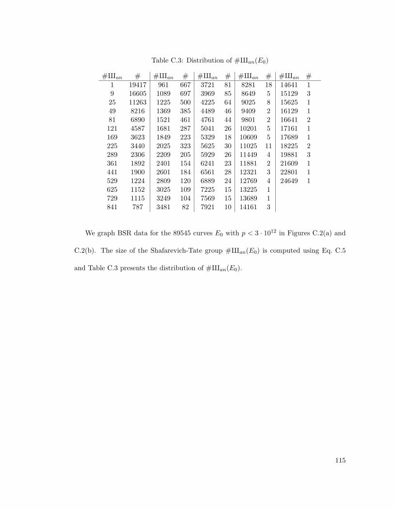
Table C.3: Distribution of #Xan(E0)

#Xan # #Xan # #Xan # #Xan # #Xan #1 19417 961 667 3721 81 8281 18 14641 19 16605 1089 697 3969 85 8649 5 15129 325 11263 1225 500 4225 64 9025 8 15625 149 8216 1369 385 4489 46 9409 2 16129 181 6890 1521 461 4761 44 9801 2 16641 2121 4587 1681 287 5041 26 10201 5 17161 1169 3623 1849 223 5329 18 10609 5 17689 1225 3440 2025 323 5625 30 11025 11 18225 2289 2306 2209 205 5929 26 11449 4 19881 3361 1892 2401 154 6241 23 11881 2 21609 1441 1900 2601 184 6561 28 12321 3 22801 1529 1224 2809 120 6889 24 12769 4 24649 1625 1152 3025 109 7225 15 13225 1729 1115 3249 104 7569 15 13689 1841 787 3481 82 7921 10 14161 3

We graph BSR data for the 89545 curves E0 with p < 3 · 1012 in Figures C.2(a) and

C.2(b). The size of the Shafarevich-Tate group #Xan(E0) is computed using Eq. C.5

and Table C.3 presents the distribution of #Xan(E0).

115

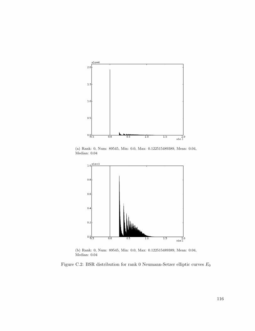
(a) Rank: 0, Num: 89545, Min: 0.0, Max: 0.122515489389, Mean: 0.04,Median: 0.04

(b) Rank: 0, Num: 89545, Min: 0.0, Max: 0.122515489389, Mean: 0.04,Median: 0.04

Figure C.2: BSR distribution for rank 0 Neumann-Setzer elliptic curves E0

116

C.3 Cremona database

The allbsd database [Cre] of J.E. Cremona lists elliptic curves of conductor upto 120, 000

along with terms appearing in the BSD conjecture. We used the regulator and the size

of the Shafarevich-Tate group of each of these curves and plotted their BSR values.

(a) Rank: 0, Num: 316414, Min: 0, Max: 0.127420362791, Mean: 0.01,Median: 0.0

117

(b) Rank: 0, Num: 316414, Min: 0, Max: 0.127420362791, Mean: 0.01,Median: 0.0

Figure C.3: BSR distribution for rank 0 elliptic curves in the Cremona database

(a) Rank: 1, Num: 394879, Min: −0.256057275686, Max:0.160553198649, Mean: 0.02, Median: 0.02


118



(a) Rank: 3, Num: 836, Min: −0.0579331293169, Max: 0.101373726334,Mean: 0.0, Median: −0.01


119

C.4 Stein-Watkins database

The database of W.A. Stein and M.J. Watkins [SW02] lists 136, 924, 520 elliptic curves of

conductor at most 108 along with L∗E(1) the leading coefficient of the Taylor expansion

of LE(s) at s = 1. For each conductor and each isogeny class the database lists the rank

and L∗E(1) and the curves in that isogeny class. (Recall that BSD conjecture is isogeny

invariant, that is, each curve in an isogeny class have the same rank and L∗E(1).)

Our SAGE script iterates through each elliptic curve E in an isogeny class and com-

putes BSR(E) by determining Reg(E) · #X(E) via the BSD formula using the L∗E(1)

value supplied by the database. The SAGE documentation notes that the Stein-Watkins

database unlike the Cremona database need not list all curves of a given conductor and

that it lists the curves whose coefficients are not too large [SW02].

(a) Rank: 0, Num: 45976073, Min: −4.76990360214e − 06, Max:0.176325563645, Mean: 0.01, Median: 0.0

120

(b) Rank: 0, Num: 45976073, Min: −4.76990360214e − 06, Max:0.176325563645, Mean: 0.01, Median: 0.0

Figure C.7: BSR distribution for rank 0 elliptic curves in the Stein-Watkins database



121





122



(a) Rank: 5, Num: 45, Min: 0.044667548058, Max: 0.132783309048,Mean: 0.09, Median: 0.08


123

I don’t know what I may seem to the world. But as to myself I seem to have been only

like a boy playing on the seashore and diverting myself now and then finding a smoother

pebble or a prettier shell than the ordinary, whilst the great ocean of truth lay all

undiscovered before me. I. Newton

124

Index

E(Q), see Mordell-Weil group

E(Q)tors, see Elliptic curve rational torsion

subgroup

L∗E(1), see leading coefficient of L-series at

s = 1

Reg(E), see Elliptic regulator

#Xan(E)

Analytic order of X(E), 110

distribution, 112, 115

Γ(s), see Gamma function

Ω, see Real period

, 40

, 40

O, 24∏p cp, see Tamagawa product

Vol(E), see Elliptic curve complex area

cp, see Tamagawa number

vp, see Valuation at p

Qp, p-adic numbers, 3

X, see Shafarevich-Tate group

AGM, see Arithmetic-Geometric Mean

al-Kashi, Ghiyath al-Din Jamshid Mas’ud,

22

Algorithm

l-adic E(Q)tors computation, 32

Baby-Step Giant-Step, 82

Chistov, 100

deciding if #E(Qp)[p] = p, 99

Doud, 24

Garcıa-Selfa et al., 24

lambda method, 82

Loos, 24

parallel E(Q)tors computation, 77

parallel determinant computation, 83

Pauli, 100

Pollard Rho, 82

radix conversion, 36

Schoof, 82

125

Schonhage-Strassen, 36

Tate, 13

time complexity, 37

van Oorschot-Wiener, 82

Arithmetic-Geometric Mean, 75, 79

Artin, E., 10

Atkin, A.O.L., 23

Babai, L., 101

Big X’s, 49

Birch and Swinnerton-Dyer conjecture, see

BSD conjecture

Birch, B.J., 18, 109

Brauer, R., 40

Brauer-Siegel

analogue for elliptic curves, 42

analogue for rank 0 elliptic curves, 42

ratio, 109, 112, 114, 117, 120

theorem for number fields, 39

BSD conjecture, 19

formula, 19

weak, 19

Canonical height pairing, 19

Cassels-Tate pairing, 17

Chistov, A.L., 100

Class number formula, 40

Coding theory, 4

Computer

meccah.math.harvard.edu, 110

sage.math.washington.edu, 110

EDSAC2, 18

Conductor, 16

Congruent number, 20

Conjecture

ABC, 43

Brauer-Siegel analogue for elliptic curves,

42

de Weger, 44

Frey-Szpiro, 43

Goldfeld-Szpiro, 43

Hall, 50

Hardy-Littlewood F, 66, 114

Hindry, 42

Lang’s bound for #X(E) ·Reg(E), 41

Riemann hypothesis, 44

Szpiro, 25, 43

126

upper bound for #X(E), 43

Connecting homomorphism, 99

Cremona database, 117

Cremona, J.E., 117

Cryptography, 4

Danilov, L.V., 50

de Weger, B.M.M., 44

Dedekind zeta function, 40

Discriminant

global minimal, 12

Division polynomial, 9

prime support, 29

Doud, D., 24

Dream Theater, ii

Elkies, N.D., 25

Elliptic curve, 5

m-torsion subgroup, 7

analytic rank, 18

complex area, 79

complex multiplication, 57

conductor, 16

coordinate transformations, 78

discriminant, 5

group law, 6

periods, 78

quadratic twist, 53, 67

quartic twists, 57

rational torsion subgroup, 23

torsion subgroup, 7

Elliptic curves

Frey-Hellegouarch, 44

Neumann-Setzer, 114

Elliptic regulator, 19, 83

Erdos, P., 101

Euler product, 15

Exact sequence, 61

long, 93, 96, 98

short, 16, 93, 96, 98

Exponential integral function, 80

Formula

BSD conjecture, 19

class number, 40

Gross-Zagier, 67

Fourier coefficients, 80

127

recurrence formulae, 81

Frobenius map, 10

trace of, 10

Galois cohomology, 16

Gamma function, 15

Garcıa-Selfa, I., 24

Gauss, C.F., 57, 79

Goldfeld, D., 43

Gross, B., 20

Gross-Zagier formula, 67

Guy, R.K., 39

Hall, M., 50

Hardy, G.H., 91

Hasse local-global principle, 4

failure, 4

Hasse, H., 10

Heegner

hypothesis, 67

index, 69

point, 67

point method, 67

sketch of time complexity, 69

Height

canonical, 83

local, 83

naıve, 63

elliptic curve, 63

Hensel lifting, 26, 99

Hensel, K., 26

Heuristics

Cohen-Lenstra, 48

random matrix theory, 48

Hindry, M., 39

Homogeneous space, 57, 107

principal, 17

Huang, M.-D., 3

Imaginary quadratic field

discriminant, 67

Heegner hypothesis, 67

trivial class group, 49

trivial class group discriminants, 49

Isogeny, 6

degree, 7

descent, 17

128

dual, 7

Katz, N.M., 38

Knuth, D.E., 32

Kolyvagin, V.A., 20, 54, 63

Kraus’ conditions, 51

Krir, M., 70

Kronecker

second limit formula, 31

Kronecker, L., 31

L-series, 15

analytic continuation, 15

convergence, 15

functional equation, 15, 63, 106

leading coefficient

bounds, 47

leading coefficient at s = 1, L∗E(1), 19

Lang, S., 4, 41

lc, see Polynomial leading coefficient

Legendre symbol, 82, 95

Lemma

Hensel, 26

snake, 93

Stark, 31

Loos, R., 24

MAGMA, 31, 74

Matplotlib/pylab, 110

Mazur, B., 23

Minimal model

global, 12

local, 12

Mordell, L.J., 10

Mordell-Weil group, 11, 84

finitely generated, 11

rank, 11

weak, 17

Multi

core, 73

processor, 73

Naıve height

elliptic curve, 41

rational point, 63

Newton, I., 124

Notation

, 40

129

, 40

O, 24

∼, 40

soft-Oh, 24

Neron-Tate pairing, 83

Oesterle, J., 38

Pairing

canonical height, 19

Cassels-Tate, 17

Neron-Tate, 83

Weil, 91

Parallel

E(Q)tors computation, 77

code, 74

determinant computation, 83

embarassingly, 75

Parent, P., 38

PARI/GP, 74, 110

Pauli, S., 100

Point at infinity, 5

Polynomial

discriminant, 9

division, 9

leading coefficient, lc, 9

Problem

class number, 49

congruent number, 20

elliptic curve discrete logarithm, 2

Rankin-Selberg zeta function, 44

Real period, 18

bounds, 47

Reduction

additive, 13, 96

bad, 13

good, 13

non-split multiplicative, 13, 96

potential good, 30

potential multiplicative, 30

split multiplicative, 13, 97

Root number, 16

global, 105

local, 81, 105

Root of unity, 99

SAGE, 74, 110

130

Schoof, R., 82

Schweitzer, A., iii

Selmer group, 17, 60

Semaev-Smart-Satoh-Araki, 2

Serre, J.-P., 38

Shafarevich-Tate group, 4, 17

analytic order, 85, 110

finiteness, 17

size, 85

size is a square, 17

trivial element, 17

Shintani-Shimura lift, 44

Silverman, J.H., 4, 59, 84

Singular point, 108

Soft-Oh, 24

Spencer, J., 101

Stark, H.M., 25, 31

Stein, W.A., 48, 72, 120

Stein-Watkins database, 120

Swinnerton-Dyer, H.P.F., 18, 109

Sylvester matrix, 12

Szpiro, L., 43

Tamagawa

number, 19, 77

bounds, 47

product, 19, 77

bounds, 47

Tate

algorithm, 13

curve, 97

module, 10

normal form, 24

Tate, J., 13, 18

Taylor expansion, 16

Theorem

Brauer-Siegel, 39

Bump-Friedberg-Hoffstein, 69

chinese remainder theorem, 82

Danilov, 50

Grosss-Zagier, 67

Hasse, 3, 10

Hecke, Wiles et al., 15

Krir, 70

Mazur, 11

modularity, 15

131

Mordell-Weil, 10

Murty-Murty, 69

Nagell-Lutz, 11

Tunnel, 20

Time complexity

l-adic E(Q)tors computation, 38

multiplying integers, 36

Tate’s algorithm, 37

Torsion subgroup

upper bounds, 38

Triangle, 20

right angled, 20

area, 20

Tunnell, J.B., 20

Updike, J., 2

Valiant, L.G., 73

Valuation at p, 12

Voloch, F., 38

Watkins, M.J., 120

Weierstrass equation, 5

Weil pairing, 91

Weil-Chatelet group, 60

Wiles, A., 3

Zagier, D., 20

Zeta function, 14

Dedekind, 40

Rankin-Selberg, 44

132

Some computational problems motivated by the Birch and Swinnerton-Dyer conjecture

Documents

Transcript of Some computational problems motivated by the Birch and Swinnerton-Dyer conjecture