HAL Id: hal-03020623https://hal.archives-ouvertes.fr/hal-03020623

Preprint submitted on 11 Dec 2020

HAL is a multi-disciplinary open accessarchive for the deposit and dissemination of sci-entific research documents, whether they are pub-lished or not. The documents may come fromteaching and research institutions in France orabroad, or from public or private research centers.

L’archive ouverte pluridisciplinaire HAL, estdestinée au dépôt et à la diffusion de documentsscientifiques de niveau recherche, publiés ou non,émanant des établissements d’enseignement et derecherche français ou étrangers, des laboratoirespublics ou privés.

Enquiry on the mainly stochastic nature of Birch andSwinnerton-Dyer’s conjecture.

Hubert Schaetzel

To cite this version:Hubert Schaetzel. Enquiry on the mainly stochastic nature of Birch and Swinnerton-Dyer’s conjec-ture.. 2020. hal-03020623

p 1/73

Number Theory / Théorie des nombres

Enquiry on the mainly stochastic nature of Birch and Swinnerton-

Dyer's conjecture.

Hubert Schaetzel

Abstract Is Birch and Swinnerton-Dyer proposal the corollary of Mertens third theorem, of the Satō-Tate

distribution and its complex multiplication colleague or of the standardization made by Kolyvagin-Gross-

Zagier ? The answer to this question is certainly that all three outcomes are essential. We propose to use

these remarkable tools to confirm Bryan Birch and Peter Swinnerton-Dyer intuition, starting with an in-

depth study of sums weighted by random variables based on the Satō-Tate and cousin distributions. The

overall effect of these distributions rests on Mertens' shoulders thanks to his theorem. Finally, the last

mentioned authors allow the calibration of the allowed steps in this very particular universe. We will not

use all of the two and a half million elliptic curves listed in the University of Warwick database combined

with extraordinary means of artificial intelligence, but that does not mean that the point clouds will not

deliver an equally clear and explicit message here.

Enquête sur le caractère essentiellement stochastique de la conjecture de Birch et Swinnerton-Dyer.

Résumé La proposition de Birch et Swinnerton-Dyer est-elle le corollaire du troisième théorème de Mertens, de la

distribution de Satō-Tate et de sa consœur à multiplication complexe ou bien de la calibration faite par

Kolyvagin-Gross-Zagier ? La réponse à cette question est assurément que les trois résultats sont

indispensables. Nous proposons de nous appuyer sur ces remarquables outils pour confirmer l’intuition de

Bryan Birch et Peter Swinnerton-Dyer en commençant par une étude approfondie de sommes pondérées

par des variables aléatoires basées sur la distribution de Satō-Tate et sa distribution cousine. L’évaluation

de l’effet d’ensemble de ces distributions repose sur les épaules de Mertens en lien avec son théorème.

Enfin, les derniers auteurs cités permettent l’étalonnage des pas autorisés dans cet univers tout à fait

particulier. Nous n’utiliserons pas l’ensemble des deux millions et demi de courbes elliptiques répertoriées

dans la base de données de l’université of Warwick allié à d’extraordinaires moyens d’intelligence

artificielle mais cela ne signifie pas que les nuages de points ne délivreront pas ici un message tout aussi

clair et explicite.

Statute Preprint

Date Version 1 : November 22, 2020

Abbreviations

If(x, y, z) If x is true then y otherwise z

And(x, y) Simultaneous condition for x and y

|v| Absolute value of v

CM Complex multiplication

p 2/73

Summary

1. General framework. 3

2. Birch and Swinnerton-Dyer conjecture statement. 5

3. Demonstration strategy. 6

4. Sums with random variables. 6

4.1. Random variable. 6

4.2. Bounded uniform random variable. 7

4.3. Near-linear growth of prime numbers. 8

4.4. Abscissas of convergence. 8

4.5. Sum of integers. 8

4.6. Alternated sum of square roots. 9

4.7. Alternated sum of powers of integers. 10

4.8. Distributions. 11

4.9. Domain of convergence associated to the distribution profiles applied to integers. 16

4.10. Domain of convergence associated to the distributions profiles applied to the prime numbers. 21

4.11. Predominance of randomness. 26

5. Theorem de Mertens. 26

5.1. Riemann series. 26

5.2. Mertens third theorem. 26

5.3. Generalization of Mertens’ theorem. 27

6. Arithmetic rank of an elliptic curve. 28

6.1. Arithmetic average. 28

6.2. Link with the Mertens theorem. 29

6.3. Equality of arithmetic and analytical rank. 31

7. Distributions relative to the quadratic opposite. 32

7.1. Situation analysis. 32

7.2. Numeric illustration. 32

7.3. Explicit formulas. 33

7.4. Spread at the two limit distributions. 34

8. Impact of copies of ℤ. 37

8.1. Recovering by error terms. 37

8.2. Calibration of the reciprocal effect of a Z copy and of rank 1. 38

8.3. Generalization to ℤn and rank n. 38

9. Conclusion. 39

10. References. 41

11. Annexe 1 : Examples of elliptic curves from rank 0 to 28. 42

12. Annexe 2 : Dispersion of a random sum. 44

13. Annexe 3 : Fisher-Yates’ shuffle algorithm. 47

14. Annexe 4 : Shuffle algorithm modulo 3. 51

15. Annexe 5 : Comparison of random sums to alternating sums of integers. 54

16. Annexe 6 : Extremums of SN(n,m,offset) sums. 56

17. Annexe 7 : Effect of Fisher-Yates algorithm on weighed prime numbers sums. 57

18. Annexe 8 : Accélération de l’effet de convergence. 62

19. Annexe 9 : Comparison of distribution 𝔇2 to its approximation. 64

20. Annexe 10 : Evolution of the average of the error term (or quadratic opposite) ap. 66

21. Annexe 11 : Deviation to the distributions. 68

22. Annexe 12 : Evolution of Euler products ratios. 72

p 3/73

1. General framework.

Introduction

The number of local solutions, i.e. modulo p, of an equation like y2-(x

3+a.x+b) = 0 follows a curious property. It would

seem natural to have, on average, p solutions for this equation by examining the results of the operations x = 0 to p-1

crossed with y = 0 to p-1 and this by proceeding to "all" checks p = 2, p = 3, p = 5, p = 7,... up to infinity. Surprisingly,

for each of these equations, there is either this average result of p solutions indeed or an excess to this average. A deficit

is excluded regardless of the choice of values and signs of the coefficients a and b. The balance is either fair or always

leans on the same side. Moreover, the gap, when it manifests, always materializes in quantum leaps. Only "orbitals" in

integer values are allowed. Even stranger, by dint of staying off the beaten track, the explanation of this phenomenon has

given rise to a formidable ransom to extract the hermetic alchemy. The purpose of this article is to revisit these

disturbing observations and participate in this heady quest of a new type of Holy Grail.

The stochastic nature of the desired result is omnipresent and requires careful developments beforehand. In reality, this

character is an opportunity because it leads to only two cases, namely two distributions related to the existence or not of

a so-called complex multiplication. This small number (only two) allows us to be visiting them at length and the theory

(of probabilities) leads to the conclusion that the offenders have zero probability. The crucial point in the thread of ideas

is a difference of 1/2 within the powers of two groups of expressions, the same real value as that of Riemann's zeros, this

having likely here nothing to do only with mere happenstance. Finally, exploring further, we will see that the jumps

observed in the rank, a property associated with each elliptical curve, have nothing of the curiosity of the phenomena of

quantum physics, but rather fall under that of copies of infinity, an impact perhaps even more mysterious.

In the sequel, the theorems of mathematical literature, although ubiquitous and essential here, are given without

rewriting the proofs. The reader can rely on references for more information. Many graphs are given in order to lighten

the arguments and theorems to which they relate.

Equation

An elliptical curve E is a particular case of algebraic curves. It admits a cubic equation in a form of so called Weierstrass

formula [23] :

y2+a1.x.y+a3.y = x

3+a2.x

2+a4.x+a6 (1)

We place ourselves here in the field of rational numbers ℚ.

In this commutative field (of characteristic 0), the equation of the elliptical curve E also admits a simplified form :

(E) y2 = x

3+a.x+b (2)

We will use this last equation for all theoretical developments.

On the other hand, the identification of numerical examples is made by the more general form [a1, a2, a3, a4, a6].

The discriminant of the simplified equation, ∆ = -16(4a3+27b

2), is an indicator of the singularities on the curve. One

refers to elliptical curves only when this discriminant is different from zero, which is therefore equivalent to the absence

of singularities.

Group law on ℚ

The essential property of elliptical curves is the existence of a geometric addition on the points of the graph. Considering

two rational points on the curve, the third point, symmetrical to the x axis of the intersection with the line passing

through the first two points, is necessarily a rational point. Similarly, the tangent line at a rational point, the latter

considered a double point, gives for a rational third point and its symmetric point, while a vertical line intercepting the

curve gives the third point to infinity, taken as neutral point 0E.

We thus have a composition law + with neutral element 0E on the elliptical curves and all of the points of the E curve,

including the infinity point, forms a commutative group.

Starting from two rational points or a rational double point, and continuing the additions on the previous two points, two

possibilities arise :

- Either at the end of a finite number of operations we return to the initial points,

- Or the number of operations continues to infinity.

p 4/73

Theorem 1 : Theorem of Mordell-Weil

The rational points (i.e. here belonging to ℚ) of the elliptical curve E(ℚ) form a finite abelian group, that is, the direct

product of a finite number r of copies of ℤ and of finite cyclic groups E(ℚ)tors

:

E(ℚ) ≃ ℤr ⊕ E(ℚ)

tors (3)

Definition 1 : Algebraic rank

The integer r = ral is called the algebraic rank of the elliptic curve.

The finite subgroups E(ℚ)tors

are called torsion groups and their characteristics are given by the Mazur theorem.

Note : The existence of torsion groups has no bearing on the rest of this text. We are only interested in the number of ℤ

copies that are solutions to the equation.

Group law on 𝔽p

Let us now consider the finite field 𝔽p = [0, 1, 2,…, p-1], p a prime number.

The group law is preserved (i.e. this time modulo p).

The number of solutions of equation E in this field is noted #E(𝔽p). Counting the point at infinity, we have :

#E(𝔽p) = 1+#(x,y) ∈ 𝔽p x 𝔽p \ y2 = x

3+a.x+b mod p (4)

We then have the following :

Theorem 2 : Hasse theorem [27]

Le cardinal of #E(𝔽p) is within the interval :

p+1-2p1/2

< #E(𝔽p) < p+1+2p1/2

(5)

One of the methods of searching for the number of solutions is the one using the Legendre symbol χ(E*) = (𝐸∗

𝑝), where

E* is the right member of the E equation given by the relation (2)

#E(𝔽p) = p+1+∑ (x3+a.x+b

𝑝)

𝑝−1𝑖=0 (6)

Definition 2

We define ap in the usual way :

ap = (-1).∑ χ(E*)𝑝−1𝑖=0 = p+1-#E(𝔽p) (7)

The ap number is the opposite of the "finite sum of Legendre" using the simplified form of Weierstrass. This integer

being regularly addressed in the article, for practical reasons, we will call it here the "quadratic opposite". We also use

the words "error term" which it often gets.

Corollary 1

The limit values of the opposite quadratic ap are given by :

-2p1/2

< ap < 2p1/2

(8)

Definition 3

Let us have L(E,s) the infinite product with parameter the complex variable s, called incomplete L function of E :

L(E,s) = ∏ (1-ap.p-s+p

1-2s)

-1 (9)

p∤2Δ

The prime numbers p that divide Δ are in finite quantity. They do not affect the expression of the elliptic curve's rank.

Therefore, we do not take that into account in our article.

p 5/73

Theorem 3 : Modularity theorem

In 2001, Christophe Breuil, Brian Conrad, Fred Diamond and Richard Taylor, extending the work of Andrew Wiles,

demonstrated that all elliptical curves on ℚ are modular [28] [3].

2. Birch and Swinnerton-Dyer conjecture statement.

Birch and Swinnerton-Dyer's conjecture can be expressed in several ways.

Statement 1

(according to reference [1])

Let us have the expansion of Taylor's series for L(E,s) at point s = 1, where c ≠ 0 and r is a positive or null integer, such

that :

L(C, s) = c.(s-1)r + terms of higher orders (10)

then integer r is equal to the algebraic rank of the elliptical curve (following definition 1 given on page 4).

Definition 4 : Analytic rank

Integer r, as defined in the relation (10), is called the analytic rank, noted ran, of the elliptic curve E in the field ℚ.

Statement 2

This is initial B. Birch and P. Swinnerton-Dyer statement.

Let us have

∏ (#E(𝔽p)-1)/p ≈ C.lnr(x) when x→ +∞ (11)

p≤ x

or also

∏ (1-ap/p) ≈ C.lnr(x) when x→ +∞ (12)

p≤ x

then the exponent r is equal to algebraic rank ral of the elliptic curve.

Remark :

Expression of the function L is close to relation (12) as :

L(E, 1) = ∏ (1-(ap-1)/p)-1

(13)

Link between statements 1 and 2.

Theorem 4 (Golfeld, 1982)

According to [11] (chapter IV, page 166) and [8], if E is modular, which is the case for any elliptic curve on ℚ according

to theorem 3, and if there exists a constant C and a number r such as ∏p≤ x (1-ap/p) ∼ C.lnr(x) when x→ +∞, then L(E,s)

∼ C’.(s-1)r when s → 1, C’ being a constant.

So we have the implication :

Statement 2 ⇒ Statement 1 (14)

It is under the first form, hence stronger, that of Euler's product, that we will conduct the presentation of this article,

using a generalization of Mertens theorem.

The two previous statements boil down to the following.

Statement 3 :

The analytic rank ran and algebraic rank ral of a given elliptical E curve are identical.

Important note

Birch-Swinnerton's conjecture is goes essential in one sense, that is, when algebraic rank is r then the multiplier factor in

the expression of Taylor's expansion is r. We will stick to this in this article, meaning that often the reader will only find

implications and not equivalencies, some of which are self-evident anyway.

p 6/73

3. Demonstration strategy.

The argument requires defining a third notion of rank that we call arithmetic rank and is noted rth.

This rank is none other than the asymptotic average of the error term ap.

It seems natural that in the absence of a forced bias, this average be zero. Of course, local ap values are strictly defined

by the coefficients [a1, a2, a3, a4, a6]. On the other hand, on a global scale, the average error term is 0 if a random walk is

at work.

Yet, the asymptotic distribution profiles of the number of solutions on 𝔽p fields is reduced to one for complex

multiplication curves (noted 𝔇1∞ profile later on) and another, also unique, for curves without complex multiplication

(𝔇2∞ profile). These profiles are symmetrical to the original. This means that the average values of the error term ap,

which we will call arithmetic rank, deviates by a finite value from value 0.

A bias can be introduced by the existence of an infinite number of solutions generated by the operation of groups’

addition for rational points on elliptical curves by modulo pk projections.

With a per unit reproducible calibrated phenomenon (r = 0 and r = 1 implying r = 2, r = 3, etc.) and a corollary of

Mertens's third theorem capable of translating the arithmetic rank into an analytical rank, the desired link is realized.

Hence Birch Swinnerton-Dyer's proposal summarized in the following implications :

Methods Results Pages Methods Results Pages

ral = 0 (≃ ℤ0) ral = 1 (≃ ℤ1

)

Theorem 31 ⇓ p 38 Theorem 31 ⇓ p 38

ran = 0 ran = 1

Theorem 27 ⇓ p 31 Theorem 27 ⇓ p 31

rth = 0 rth = 1

Proposition Erreur ! Source du renvoi introuvable. ⇓

rth → rth +1 (≃ ℤn)

Theorem 36 ⇓ p 39

rth = n

Theorem 27 ⇓ p 31

ran = n

Theorem 26 ⇓ p 29

ral = n

These implications do not have an obligation to be studied in the previous order and are not.

4. Sums with random variables.

We study these sums because the error terms ap take in their domain of definition values whose behaviour can be

described as random. The purpose of the elements gathered under this first paragraph will be to see to what extent such

(random) behaviour would suffice to realize Birch Swinnerton-Dyer's conjecture.

4.1. Random variable.

According to the reference [17], the definition of a random variable, a definition that extends to functions of random

variables, is as follows :

Definition 5 : Random variable

Let us have (Ω,F,ℙ) a probabilized space and (E,𝜖) a measurable space. We call random variable from Ω to E, any

measurable function X from Ω to E. The measurement ℙX is the image, by the X-application, of the probability ℙ set on

(Ω,F).

The purpose is not here to start a course on probability theory. We are therefore not going to repeat explanation one can

find elsewhere on the previous terms. The only word we are interested in is "measurable" and let us first note that our

measurements will be taken on the set E = ℜ.

We can characterize a random variable by properties.

p 7/73

Characteristic 1

A random variable X has moments, i.e. expected values, such as the mean value E(X), the variance V(X), standard

deviation σ(X), and so on.

Characteristic 2

A random variable X, and similarly a continuous and derivable function of a random variable, meets criteria for the

reproducibility of its image, i.e. results of calculations, reproducibility that improves with the repetition of experiments.

For the realization of these calculations, the random variable, abstract object, is replaced by an estimator of X. (ref.

[18]). The image obtained from an unbiased estimator is true to the expected image, within the expected deviations,

when these are available data. A random variable, and its estimator, despite the qualifying adjective used, is therefore

not unpredictable. On the contrary, its random nature assigns it remarkable laws of regularity and symmetry.

Thus the image of an n-steps experiment is asymptotically close to predictable data. The results of several tests take

values that deviate less and less from a given framework as the number of experiments or tests increases. The result of a

single experiment is indeed random (eventually limited to an interval), but the result of many trials is getting closer and

closer to a given framework that is perfectly definable and measurable.

That is why, in the sequel, we rely on an increasing number of data to deduce asymptotic data from the variable or

random function studied.

To recognize certain characteristics, we have to use an indispensable tool : sorting by increasing values.

Definition 6 : Distribution

We call distribution the results vi of n experiments sorted by increasing values.

The world of probabilities, being by essence the world of randomness, nothing could not be said about anything, without

starting from a minimal axiom of expected image (or distribution) for a large number of tests and repeatability of this

image (or distribution).

The repetition of images of random tests converging towards a given distribution is assumed to be the premise of the

asymptotic image of that distribution.

Definition 7

According to the usual definition, we say that an event is almost sure if its probability is 1. In other words, the set of

cases where the event does not occur has a probability 0.

4.2. Bounded uniform random variable.

All the random functions in this text are constructed from a bounded uniform variable.

Definition 8 : Bounded uniform random variable

A bounded uniform random variable is at once random, uniform and admits lower and upper bounds. The second term

means that its distribution function is linear. Its probability density is therefore a constant.

The generating function Mx of the moments of this variable allows calculating all the moments of this variable (see

reference [19]).

Bates Law

Bates Law is the law of probability of the arithmetic average of random n variables u1, u2,... ,um, of continuous uniform

law on interval [0,1] (reference [20]).

Theorem 5

The variance in the mean value of m variables ui is equal to 1/(12m) (reference [20]).

The standard deviation is therefore :

σ(uim) = (1/12m)1/2

(15)

We rely for all the data and graphs of this text on the uniform pseudo-random variable available on Excel spreadsheet.

This one is bounded to [0,1]. Its average value is 1/2, its standard deviation is (1/12)1/2

and its distribution (which is also

p 8/73

its distribution function) is linear between 0 and 1. It is called "pseudo-random" since it is a concrete object, and

therefore an estimator, and so may not be implemented in a perfectly random way.

4.3. Near-linear growth of prime numbers.

Theorem 6

The asymptotic growth rate of ln(pi) is slower than iε, regardless of the initial choice of ε > 0.

lim

i → +∞

ln(pi) = 0 (16)

iε

Proof

Very briefly, function ln(pi) is concave while function iε is convex. Hence the result.

A longer reasoning is based on a well-known result : the term ln(i) asymptotically grows slower than any exponential,

i.e. ∀ ε > 0, ln(i)/iε → 0

+. Of course, it also means that ln(i)/i → 0

+ when i → +∞. Substituting to the term i the term ln(i),

we have asymptotically ln(ln(i))/ln(i) → 0+, then ln(ln(ln(i)))/ln(ln(i)) → 0

+, and so on. As i tends to infinity each of the

terms ln(ln(ln(i))...) gets negligible in front of his predecessor ln(ln(i)...). The sum ln(i)+ln(ln(i))+ln(ln(ln(i)))+ … +

ln(ln(…ln(ln(pi))) is growing with increasingly smaller terms. So there is k > 0 such as for i > k, ln(pi) < 2ln(i). Besides a

numerical check shows that this result is true for any i. So ln(pi)/iε/2 < ln(i)/i

ε → 0

+, when i → +∞.

Theorem 7

The asymptotic growth rate of pi is slower than i1+ε

, regardless of the initial choice of ε > 0.

lim

i → +∞

pi = 0 (17)

i1+ε

Proof

Asymptotically we have, according to Legendre's rarefaction theorem, pi → i.ln(pi). The result is pi/i1+ε

= pi/i/iε →

ln(pi)/iε → 0

+, when i → +∞ according to the previous theorem.

Corollary 2

The theorem is equivalent to say that pi asymptotically grows barely faster than i, and hence that ∀ ε > 0, there is k such

as pi < i1+ε

for any i > k.

Note :

The inversion between pi and i1+ε

occurs around ε ≈ 0,42 for i = 10, ε ≈ 0,187 for i = 100, ε ≈ 0,128 for i = 1000, ε ≈

0,096 for i = 10000, ε ≈ 0,077 for i = 100000, or approximately between i = 10 and i = 100000, ε ≈ 13/30/ln(ln(i))-1/10.

4.4. Abscissas of convergence.

Theorem 8

Let us have η(s) the Dirichlet Eta function defined on a complex plane

+∞

η(s) = ∑ (-1)i-1

1

(18) is

i = 1

The Dirichlet Eta function converges simply for real numbers s ≥ 0 and diverges if s < 0 (reference [25]).

The same is true if i is replaced by pi because of theorem 7.

What will interest us later is the position of this convergence radius when (-1)i-1

is replaced by a random variable without

bias taking values this time within the whole interval [-1, 1] instead of the boundaries values -1 and 1 only.

4.5. Sum of integers.

We get the alternated sum from the non-alternated sum. So we start with the latter.

p 9/73

Theorem 9

Let us have the following sum where k is a positive integer :

m

S(k,m) = ∑ ik (19)

i = 1

We have the recurrence relationship (reference [16]) :

k+1

(k+1).S(k,m) = (m+1)k+1

-1- ∑ (𝑘+1𝑖

) S(k+1-i,m) (20)

i = 2

For example, from S(0,m) = m, we get S(1,m) = m.(m+1)/2 and S(2,m) = m.(m+1).(2m+1)/6.

All calculations made, we have from [15] :

k

S(k,m) = ∑ Bi .

k! . (m+1)

k+1-i (21)

i! (k+1-i)!

i = 0

The first terms of the expression are thus given by :

S(k,m) = 1

(m+1)k+1

- 1

(𝑘 + 1

1) (m+1)

k+

1 (

𝑘 + 1

2) (m+1)

k-1-

1 (

𝑘 + 1

4) (m+1)

k-3 +

1 (

𝑘 + 1

6) (m+1)

k-5 -… (22)

k+1 2 6 30 42

Thus, the sum of the generic term becomes a term with an increased power of 1 :

S(k,m) = (1/(k+1)).mk+1

.(1+0(1)) (23)

This extends to the non-integer powers by Abel's summation.

4.6. Alternated sum of square roots.

The Abel summation (see reference [14] chapter I.0) gives the transformation of a sum into an integral plus an error

term. To the first order, we have :

√1+√2+…+√m = (2/3).m3/2

.(1+0(1)) (24)

Several boundary values of this sum can be given :

for m > 1

(2/3).(m)3/2

≤ √1+…+√m ≤ (2/3).(m+1)3/2

-1 (25)

for m > 0

(2/3).m.(m+5/4)1/2

≤ √1+…+√m ≤ (2/3).m.(m+3/2)1/2

(26)

or

(1/3).(m3/2

+(m+1)3/2

-1) ≤ √1+…+√m ≤ (2/3).m.(m+3/2)1/2

(27)

The latter is of very good quality. An even better choice is the following development :

m

∑ √i = (2/3).m3/2

+(1/2).m1/2

+ξ(-1/2)+0(1) (28)

i = 1

where ξ(-1/2) ≈ -0,2078862249773545660173067254 (see Pari gp).

The reader will be able to find a more complete limited development of this expression in reference [29] page 22 and

verify that the error term is less than 1/(24√m).

We then deduce, taking care to stop at the same m-rank terms, the alternating sum √1-√2+√3-√4+…+(-1)m-1

√m by

subtracting to √1+√2+√3…+√m, the sum 2(√2+√4+√6+…+√(2.⌊m/2⌋). Let us have in addition √1-√2+-…+(-1)m-1

√m

= ((2/3).m3/2

+(1/2).m1/2

+ξ(-1/2))-2√2((2/3).⌊m/2⌋3/2 +(1/2).⌊m/2⌋1/2

+ξ(-1/2))+0(1).

So that :

p 10/73

√1-√2+√3-√4+-…+(-1)m-1

√m

=

if(m = 0 mod 2,

-(1/2).m1/2

+(1-23/2

).ξ(-1/2)+ε,

m1/2

-(1/2).(m-1)1/2

+(1-23/2

).ξ(-1/2)+ε)

(29)

where ε → 0 when m → +∞.

Almost equivalently, we also have :

Theorem 10

lim √1-√2+√3-√4+-…+(-1)m-1

√m = (-1)m-1

.(1/2).m1/2

+(1-23/2

).ξ(-1/2) (30)

m → +∞

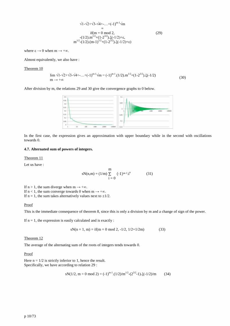
After division by m, the relations 29 and 30 give the convergence graphs to 0 below.

In the first case, the expression gives an approximation with upper boundary while in the second with oscillations

towards 0.

4.7. Alternated sum of powers of integers.

Theorem 11

Let us have :

m

sN(n,m) = (1/m) ∑ (-1)m-1.in (31)

i = 0

If n > 1, the sum diverge when m → +∞.

If n < 1, the sum converge towards 0 when m → +∞.

If n = 1, the sum takes alternatively values next to ±1/2.

Proof

This is the immediate consequence of theorem 8, since this is only a division by m and a change of sign of the power.

If n = 1, the expression is easily calculated and is exactly :

sN(n = 1, m) = if(m = 0 mod 2, -1/2, 1/2+1/2m) (33)

Theorem 12

The average of the alternating sum of the roots of integers tends towards 0.

Proof

Here n = 1/2 is strictly inferior to 1, hence the result.

Specifically, we have according to relation 29 :

sN(1/2, m = 0 mod 2) = (-1)m-1

.(1/2)/m1/2

-(23/2

-1).ξ(-1/2)/m (34)

p 11/73

4.8. Distributions.

General framework

Let us have ai = alea() a random uniform variable in the interval [0,1].

We study the point clouds Ω derived from numerical simulations of three types of distributions 𝔇0, 𝔇1 et 𝔇2 by taking

samples of increasing sizes imax = 100, imax = 1000, imax = 10000 and sometimes imax = 100000. The simulations to be

studied bear on prime numbers, but it is useful to first conduct a study based on integers and then to draw results from

appropriate comparisons. Thus the review of the 𝔇0-linear distribution of the table below is essential to the continuation

of the article.

Table 1

Distributions Formulas giving point cloud Ω Profiles vi

𝔇0-linear (1/imax) ∑i if(vi < 0, ⌈2.in⌉, ⌊2.in⌋).vi vi = 2a i-1 𝔇0 (1/imax) ∑i if(vi < 0, ⌈2.pi

n⌉, ⌊2.pin⌋).vi vi = 2a i-1

𝔇1 (1/imax) ∑i if(vi < 0, ⌈2.pin⌉, ⌊2.pi

n⌋).vi vi = sin(2π.ai).if(pi = 3 mod 4, 0, 1) 𝔇2 (1/imax) ∑i if(ai < 0, ⌈2.pi

n⌉, ⌊2.pin⌋).vi vi = cos(π.f

-1(ai)) where f(ai) = ai-sin(2π.ai)/(2π)

Note 1 : To the first case, we can also add 𝔇1-linear and 𝔇1-linear distributions using the vi profiles associated with 𝔇1 and 𝔇2.

Note 2 : There are actually two distributions 𝔇1a and 𝔇1b to be consider, one with the condition if(pi = 3 mod 4, 0, 1),

the other using the condition if(pi = 5 mod 6, 0, 1). However, their profile is the same since asymptotically, there are as

many prime numbers 1 modulo 4 and 3 modulo 4 on the one hand as 1 modulo 6 and 5 modulo 6 on the other hand. The

choice of "if (pi = 3 mod 4, 0, 1)" is thus interchangeable with "if(pi = 5 mod 6, 0, 1)" without any particular problem and

we have systematically opted for the first case.

Note 3 : A sum of functions including random variables necessarily has some dispersion. The ratio of a sum for some ith

and i+1th

tests, is not equal to 1. Appendix 2 describes the dispersal graphs expected in multiple trials on a priori

"identical" sums.

Note 4 : For numeric applications focusing on 𝔇2, we used an approximate substitute of sufficient quality to make it

easier to handle the data. This is vai = cos(arcsin(c.((1-ai).ai)ln(c)/ln(4)

)).if(ai < 1/2, -1, 1). The value of c is defined here by :

∫ (1 − c². (x(1 − x))ln(c)/ln(2)). dx

1

0 = 1/4 (35)

and is valued approximately c ≈ 1,542107446 using Pari gp (see programming inn appendix 9), hence also ln(c)/ln(4) ≈

0,312451644 and ln(c)/ln(ln)2 ≈ 0,624903288. The choice of the value of c is made in such a way to have the standard

deviation for the vi profile of the 𝔇2 distribution below :

Theorem 13 : Mean values and variances

Asymptotic averages and variances in Table 1 profiles are given by :

Table 2

Distributions Profiles vi Mean values Variances Standard

deviations

𝔇0∞ vi = 2a i-1 0 1/3 1/√3

𝔇1∞ vi = sin(2π.ai).if(pi = 3 mod 4, 0, 1) 0 1/4 1/2

𝔇2∞ vi = cos(π.f

-1(ai)) where f(ai) = ai-sin(2π.ai)/(2π) 0 1/4 1/2

𝔇2∞ approx vi = cos(arcsin(c.((1-ai).ai)ln(c)/ln(4)

)).if(ai < 1/2, -1, 1) 0 1/4 1/2

Note : We added the ∞ index to the distributions to express that they are those obtained when the sample is of infinite

size (imax → +∞).

p 12/73

Proof

Each of the formulas is symmetrical to the ordinate 0 (see also graph 1). Their average value is therefore 0. The variance

V is then given by the asymptotic limit of ∑ vi²/n for i = 1 to n, which here amounts to taking the integral from 0 to 1 for

ai in the interval [0,1].

For 𝔇0∞, ∫ (2x − 1)². dx1

0 = 1/3. We can also simply infer this from Bates' Law (see relationship 15).

For 𝔇1∞, the reader can have a look of the distribution on graph 1 below. The variance is equal to ∫ sin²(2πx). dx1/4

0 +

∫ sin²(2πx). dx1

3/4 = (1/4).(1/2)+(1/4).(1/2) = 1/4.

Pour 𝔇2∞, we have V = ∫ cos²(π. g(y)). dy1

0 where x = g(y), so that y = f(x) = x-sin(2π.x)/(2π), hence also dy = (1-

cos(2π.x)).dx. Then, the values of the integral boundaries remaining the same while changing variable y to x, V =

∫ cos²(π. x). (1 − cos(2π. x)) . dx1

0 = (1/2)∫ (1 + cos(2π. x)). (1 − cos(2π. x)) . dx

1

0 = (1/2)∫ sin²(2π. x)) . dx

1

0 =

(1/2).(1/2) = 1/4.

For 𝔇2∞ approx, the variance ∫ cos²(arcsin (c. (x(1 − x))ln(c)/ln(4)). dx1

0 = ∫ (1 − c². (x(1 − x))ln(c)/ln(2)). dx

1

0 is therefore

equal to 1/4 according to the relationship (35) defining the parameter c.

Graphical representation of profiles

The graphs below are designed from 10000 samples (imax = 10000) and an ascending sorting of results.

Types 𝔇1 and 𝔇2 distributions have not been chosen arbitrarily as we will see later on. They are related to elliptical

curves. The purpose of the 𝔇0 distribution profile, on the other hand, is to show the predominant role of randomness,

rather than the specific 𝔇1 and 𝔇2 profiles themselves, on the convergence conditions of expressions.

We will note later on the observation of similar results for 𝔇1 and 𝔇2 although these profiles are further apart than 𝔇0

is from 𝔇2. The specific virtue that brings them together is of course the identity of variances (in addition to the average

values).

Graph 1

Graphical representation of distributions

We now refer to the point clouds Ω obtained from the 2-column formulas in table 1 and proceed to 10000 tests giving

10000 different values for each of these sums (weighted by 1/imax).

For the 𝔇1 distribution, the point clouds Ω of the 10000 points thus obtained for n = 0,25 and n = 0,5 respectively are

presented below, the 𝔇0 and 𝔇2 distributions having substantially identical point clouds.

During each simulation, as the number of tests is finite, a small bias bk = (1/imax) ∑i ai is present. A point within the point

cloud shown here corresponds in abscissa to the value of this bias for experiment number k and along the ordinate to the

value Ω of the sums studied (see formulas of table 1).

The pale blue dots clouds correspond to the data where imax = 100, those in light blue to those where imax = 1000 and

those in dark blue to those where imax = 10000. When the 100, 1000 or 10000 tests are renewed, the point clouds remain

similar.

p 13/73

Graphs 2 et 3

The results we are interested in here are those for zero bias (abscissa b(k) = 0).

We observe that, for n = 1/4, the point cloud contracts on ordinate line, at the 0 bias level, when imax increases. This

means that the studied sum actually tends in the absence of bias towards 0 asymptotically. The point cloud thus

converges towards the point (0.0) when the term imax tends towards infinity.

For n = 1/2, the range of point clouds according to ordinate line remains of the same order of magnitude as imax

increases.

For n = 3/4, which we have not reported here, there is a very clear increase in the clouds of points in all directions with

the increase in imax.

Basically, we have therefore identified, close to n = 1/2, the existence of a limit case for convergence. To confirm this

value, we can, still remaining for the time being in the context of numerical tests, check the evolution of dispersion (i.e.

the standard deviation) according to n and imax. When the evolution of imax (by decade as here for example) no longer has

an effect on the evolution of n, the value of the limit case is reached.

The reader will thus find below the evolution according to n of the standard deviation σ of all the ordinate points of the

entire point cloud Ω, which gives a good assessment of what is happening at abscissa 0 corresponding to the absence of

bias.

Distribution 𝔇0-linear

n imax = 100 imax = 1000 imax = 10000 imax = 100000 Graph 4

0 0,0704 0,0224 0,0070 0,0022

0,1 0,127 0,054 0,023 0,009

0,2 0,207 0,110 0,057 0,030

0,3 0,327 0,214 0,139 0,089

0,4 0,505 0,417 0,337 0,273

0,45 0,634 0,579 0,529 0,468

0,475 0,702 0,691 0,650 0,616

0,5 0,779 0,806 0,806 0,814

0,6 1,196 1,531 1,957 2,441

0,7 1,846 3,014 4,699 7,396

0,8 2,854 5,720 11,203 22,532

0,9 4,37 10,88 27,32 69,05

1 6,64 21,20 65,77 209,06

p 14/73

Distribution 𝔇0

n imax = 100 imax = 1000 imax = 10000 imax = 100000 Graph 5

0 0,0713 0,0224 0,0072 0,0022

0,1 0,156 0,068 0,029 0,012

0,2 0,294 0,169 0,093 0,049

0,3 0,538 0,401 0,282 0,194

0,4 0,974 0,935 0,852 0,731

0,45 1,324 1,445 1,478 1,447

0,475 1,524 1,799 1,953 2,067

0,5 1,740 2,190 2,565 2,898

0,6 3,124 5,114 7,782 11,079

0,7 5,635 12,134 23,586 43,313

0,8 10,178 28,302 71,819 171,998

0,9 18,53 68,09 218,94 674,74

1 33,49 157,44 673,46 2661,30

Distribution 𝔇1

n imax = 100 imax = 1000 imax = 10000 imax = 100000

Graph 6

0 0,0559 0,0183 0,0057 0,0018

0,1 0,138 0,060 0,026 0,011

0,2 0,253 0,147 0,081 0,044

0,3 0,456 0,354 0,245 0,166

0,4 0,834 0,813 0,730 0,647

0,45 1,125 1,250 1,280 1,258

0,46 1,177 1,338 1,428 1,461

0,47 1,250 1,499 1,588 1,658

0,48 1,326 1,608 1,802 1,898

0,49 1,410 1,767 2,001 2,173

0,5 1,473 1,897 2,208 2,495

0,6 2,641 4,521 6,655 9,777

0,7 4,801 10,503 20,509 37,777

0,8 8,581 24,578 62,242 148,215

0,9 15,48 57,84 188,89 581,29

1 28,18 140,24 588,67 2303,40

Distribution 𝔇2 (approx)

n imax = 100 imax = 1000 imax = 10000 imax = 100000

Graph 7

0 0,0632 0,0202 0,0063 0,0020

0,1 0,135 0,059 0,025 0,011

0,2 0,253 0,146 0,082 0,043

0,3 0,468 0,350 0,246 0,169

0,4 0,854 0,840 0,747 0,649

0,45 1,147 1,257 1,302 1,277

0,46 1,215 1,372 1,457 1,456

0,47 1,268 1,482 1,635 1,690

0,48 1,380 1,627 1,829 1,916

0,49 1,422 1,758 2,022 2,225

0,5 1,531 1,924 2,261 2,525

0,6 2,752 4,547 6,819 9,798

0,7 5,037 10,700 20,755 38,952

0,8 8,915 24,813 63,063 151,504

0,9 16,12 58,53 190,30 592,21

1 29,35 138,68 592,36 2385,38

Abscissas of the intersections between curves are given below. As an example, we added a zoom on the values for the

𝔇1 distribution.

p 15/73

Table 3

Abscissas of intersections n

𝔇-linear

n 𝔇0

n 𝔇1

n 𝔇2

Intersection 1 : (imax = 100, imax = 1000) ≈ 0,486 ≈ 0,417 ≈ 0,413 ≈ 0,409

Intersection 2 : (imax = 1000, imax = 10000) ≈ 0,500 ≈ 0,450 ≈ 0,440 ≈ 0,438

Intersection 3 : (imax = 10000, imax = 100000) ≈ 0,498 ≈ 0,458 ≈ 0,456 ≈ 0,461

Graphics 8 et 9

These charts and graphs give an approximate idea of the convergence radius nc, power assigned to pi, for an increasing

number of tests and an increasing choice of sample sizes (m = imax). The reversal of the convergence behaviour is close

to these values.

For an exponent n less than this abscissa nc, the standard deviation tends towards 0 asymptotically following the example

of the point clouds given in graph 2.

This last table shows the gradual increase of the convergence radius towards the limit value n = 1/2 for the three

distributions 𝔇0, 𝔇1 and 𝔇2. The values are comparable but subject to uncertainty of measurement. The evolution for 𝔇0 does not seem to actually grow rapidly enough towards 1/2, but it does matter here because it is not a useful case later on. Similarly the evolution of n for 𝔇1, to some extent, is too slow. On the other hand, the evolution for 𝔇2 seems to be geared towards exceeding this value. Taking the average of the n-values for 𝔇1 and 𝔇2distributions, we can propose the following table, which shows despite the uncertainties encountered, that the assumed target is a priori the right one.

Table 4

Types of

evaluation Abscissas of intersections

n

𝔇1/𝔇2 Δn

Observed data

Intersection 1 : (imax = 100, imax = 1 000) ≈ 0,411

Intersection 2 : (imax = 1 000, imax = 10 000) ≈ 0,439 +0,028

Intersection 3 : (imax = 10 000, imax = 100 000) ≈ 0,4585 +0,0195

Plausible

numeric

simulation

Intersection 4 : (imax = 100 000, imax = 1 000 000) ≈ 0,4718 +0,01327

Intersection 5 : (imax = 1 000 000, imax = 10 000 000) ≈ 0,4808 +0,00903

Intersection 6 : (imax = 10 000 000, imax = 100 000 000) ≈ 0,4869 +0,00614

Intersection 7 : (imax = 100 000 000, imax = 1 000 000 000) ≈ 0,4911 +0,00418

Intersection 8 : (imax = 1 000 000 000, imax = 10 000 000 000 ) ≈ 0,4940 +0,00284

… … …

+∞ → 0,5

The exponent n = 1/2 being that of the Hasse formula (see theorem 2), there is not too much missing to have here an

easy game even if it is not yet won.

There remains of course one step further to be made, that of a proof, which is given later on.

Definition 9

We call the intermediate event between divergence and convergence, the "turnaround situation."

p 16/73

Theorem 14

The turnaround situation necessarily corresponds to a one-off value of the offset.

Proof

This is a trivial corollary of theorem 11.

4.9. Domain of convergence associated to the distribution profiles applied to integers.

We begin with a digression on a problem that should be simpler, which is the one where we look at integers, before

going back to the problem that we are really interested in, which is the one involving prime numbers.

Let us have

m

NSN(n, m) = (1/m) ∑ vi.in (36)

i = 0

The vi = 2.ai-1 variable is again the uniform random variable centred on 0, of definition domain [-1,1], given in Table 1.

Factor 2, used in that table, is omitted here, having no impact on the result.

We are looking for the domain n of simple convergence of this expression when m → +∞.

Let us have then the ratio :

TN(n, m, offset1) =

m

(37)

(1/m) ∑ (-1)i-1.in+offset1

)

i = 0

m

(1/m) ∑ in )

i = 0

Theorem 15

The ratio TN(n, m, offset1 = 1) tends towards ±(n+1)/2 when m tends towards infinity.

TN(n, m → +∞, 1) → (-1)m-1

.(n+1)/2 (38)

Proof

Let us write in the form of numerator and denominator TN(n, m, 1) = NTN(n, m, 1)/DTN(n, m). We then have NTN(n, m, 1) = DTN(n+1, m)-2.2

n+1.DTN(n+1, ⌊m/2⌋).

Having an alternating sum, we take good care here to develop numerator and denominator at the same rank i = m, hence a calculation restraint to the integer part of m/2 = if(m = 0 mod 2, m/2, (m-1)/2) for the second term to the right of the equality. Let us note that DTN(n, m) is none other than (1/m).S(n, m) based on the relationship (19). We then use the development (22) up to the second term, thus DTN(n+1, m) = (1/m).((m+1)n+2/(n+2)).(1-(1/2).(n+2)/(m+1)).(1+o(1)). The reader will note here that the first factor 1/m is a simple multiplier ratio. It does not interfere in the calculation of S(n, m). Let us suppose m odd to simplify further writing of equations. We get then m.NTN(n, m, 1) = m(DTN(n+1, m)-2

n+2.DTN(n+1, ⌊m/2⌋)) =

(1+o(1)).(1/(n+2)).[(m+1)n+2.(1-(1/2).(n+2)/(m+1))-2n+2.(⌊m/2⌋+1)n+2.(1-(1/2).(n+2)/(⌊m/2⌋+1))] = (1+o(1)).(1/(n+2)).[(m+1)n+2.(1-(1/2).(n+2)/(m+1))-2n+2.((m+1)/2)n+2.(1-(1/2).(n+2)/((m+1)/2))] = (1+o(1)).(1/(n+2)).[(m+1)n+2.(1-(1/2).(n+2)/(m+1))-(m+1)n+2.(1-(1/2).(n+2)/((m+1)/2))] = (1+o(1)).(1/(n+2)).(m+1)n+2.(-(1/2).(n+2)/(m+1)-(-(1/2).(n+2)/((m+1)/2))) = (1+o(1)).(1/(n+2)).(m+1)n+2.(1/2).(n+2)/(m+1) = (1+o(1)).(1/2).(m+1)n+1. This then gives by resuming the development (22) at the first term : TN(n, m, 1) = m.NTN(n, m, 1)/(m.DTN(n, m)) = (1/(n+1)).(m+1)n+1/((1+o(1)).(1/2).(m+1)n+1) = (1+o(1)).2/(n+1). A similar calculation gives the same result with opposite sign for m even. Hence the result. This expression remains true for n not being an integer (by Abel's summation).

p 17/73

Theorem 16

The ratio TN(n, m, offset1) diverges towards +∞ if offset1 > 1 and converges towards 0 if offset1 < 1.

Proof

We go back to S(n, m) = (1/(n+1)).mn+1

.(1+0(1)), from which we draw S(n+ε, m)/S(n, m) = mε.(1+0(1)). A fluctuation of

the previous offset1 within the numerator only, 1 → 1+ε, causes the ratio TN(n, m, offset1) to vary as mε.

Hence the result.

If n = 0, the denominator is equal to 1. In addition, it is easy to verify that, in this case, the numerator is equal to ±1/2

and the term TN(n, m,offset1 = 1/2) is equal to ±1/2 if offset1 = 1, diverges to +∞ if offset1 > 1 and converges to 0 if

offset1 < 1.

If n = 1, the denominator is equal to (m+1)/2. In addition, it is easy to verify that the numerator is equal to ±(m+1)/2 if

offset1 = 1 and the term TN(n, m, offset1 = 1) is equal to (-1)i-1

. Then the ratio TN(n, m, offset1) diverges to +∞ if

offset1 > 1 and converges towards 0 if offset1 < 1.

Theorem 17

The domain of convergence n of the asymptotic distribution 𝔇0-linear is n ∈ ]-∞,1/2[.

Proof

Let us consider the ratio :

RN(n, m, offset0) =

m

(39)

(1/m) ∑ v_alei.in )

i = 0

m

(1/m) ∑ in+offset0

i = 0

If valei = 2.alea()-1, this term valei takes an average value equal to 0 with a standard deviation 1/(3m)1/2

according to

Bates' law. This standard deviation follows the evolution of m and is reflected "locally" in each i by a contribution

proportional to 1/i1/2

. We then have at the limit between convergence and divergence a term 1/i1/2

that is necessarily

proportional to ioffset0

, hence offset0 = -1/2. The expression RN(n, m, offset0) will then tend towards +∞ if offset0 < -1/2

and towards 0 if offset0 > -1/2 when m → +∞ and this ∀n.

Then let us look at the ratio RN(n, m, offset0)/TN(n, m, offset1), which is none other than SN(n, m, offset

=offset0+offset1) where v_alti = (-1)i-1

and :

SN(n, m, offset) =

m

(40)

(1/m) ∑ v_alei.in )

i = 0

m

(1/m) ∑ v_alti.in+offset

i = 0

Using the theorems [15] and [16] and the previous argument on offset0, the turnaround situation is therefore located at

offset = offset1+offset0, hence offset = -1/2+1 = 1/2.

Theorem 18

The term SN(n, m → +∞, offset = 1/2) is bounded.

Proof

If offset < 1/2, the term tends towards 0. If offset > 1/2, the term diverges. However, the "offset = 1/2" case does not

necessarily result in an intermediate situation. Any result between 0 and infinity remains possible. Only the actual study

of the case, illustrated below, can be conclusive. It shows that the term SN(n, m → +∞, offset = 1/2) is of the form

c.arcsin(x). The arcsin function is bounded. The only possibility of divergence is then that c diverges what is only

possible if the curve represented by graph 10 is the vertical in 0 (equation x = 0) which it is obviously not.

Illustration of the theorem and other numerical results

The graphs representative of the distributions SN (n, m → +∞, offset) are as follows for n = 1/2 and offset = 1/2 :

p 18/73

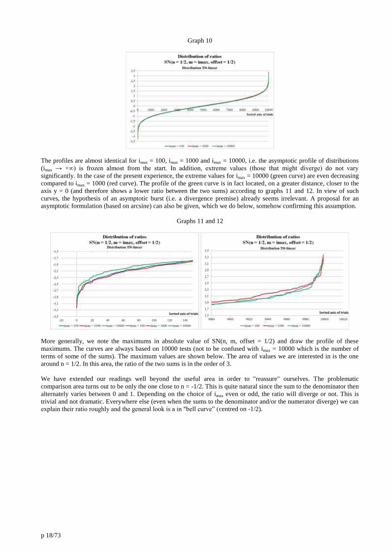
Graph 10

The profiles are almost identical for imax = 100, imax = 1000 and imax = 10000, i.e. the asymptotic profile of distributions

(imax → +∞) is frozen almost from the start. In addition, extreme values (those that might diverge) do not vary

significantly. In the case of the present experience, the extreme values for imax = 10000 (green curve) are even decreasing

compared to imax = 1000 (red curve). The profile of the green curve is in fact located, on a greater distance, closer to the

axis y = 0 (and therefore shows a lower ratio between the two sums) according to graphs 11 and 12. In view of such

curves, the hypothesis of an asymptotic burst (i.e. a divergence premise) already seems irrelevant. A proposal for an

asymptotic formulation (based on arcsine) can also be given, which we do below, somehow confirming this assumption.

Graphs 11 and 12

More generally, we note the maximums in absolute value of SN(n, m, offset = 1/2) and draw the profile of these

maximums. The curves are always based on 10000 tests (not to be confused with imax = 10000 which is the number of

terms of some of the sums). The maximum values are shown below. The area of values we are interested in is the one

around n = 1/2. In this area, the ratio of the two sums is in the order of 3.

We have extended our readings well beyond the useful area in order to "reassure" ourselves. The problematic

comparison area turns out to be only the one close to n = -1/2. This is quite natural since the sum to the denominator then

alternately varies between 0 and 1. Depending on the choice of imax even or odd, the ratio will diverge or not. This is

trivial and not dramatic. Everywhere else (even when the sums to the denominator and/or the numerator diverge) we can

explain their ratio roughly and the general look is a in "bell curve” (centred on -1/2).

p 19/73

Graphs 13, 14 et 15

The small fluctuations in the curves for n > 2 are simply due to the fact that we studied only a small number of cases n,

the drawing being automatically smoothed.

Appendix 6 provides the actual numerical data.

Returning to arbitrary n, the mere observation shows that the appropriate deviation to adopt is roughly offset = 1/2.

Indeed, by moving away from it (offset = 1/4 and offset = 3/4), the distribution of the results presented below shows

extremums that evolve with the values of imax (instead of stabilizing).

Graphs 16 et 17

When offset << 1/2 (graph 16’s example), the representative curve of the ratio SN(n = 1/2, m, offset) and its extremums

increase with the increase in m. Extremal values diverge when m → +∞. Conversely, the extreme values converge to 0

when offset >> 1/2 (graph 17’s example).

The approximate value of the offset can be confirmed, with a few additional calculations. Tight framing within 0,49 to

0,51 range is quite easy to obtain. Given the equations aspect, the wacky convergence radius like 1/2+ε, where ε would

be a little bizarre number, is not credible. However, it is not entirely unthinkable at this stage in the case of the use of

prime numbers instead of whole numbers, a point we are looking at later on.

p 20/73

Back on the numerator

Let us write SN(n, m, offset) = NSN(n, m, offset)/DSN(n, m, offset) with numerator and denominator as defined by

relation (40). The graphs in appendix 5 illustrate the previous link to convergence when offset = 1/2 (including when the

sums diverge) for NSN(n, m, offset). In the event that the alternating series diverges, however, the corresponding

random sum may eventually return to 0 in the numerical simulation (of finite size). These graphs are examples and

uniquely this.

As the vi variable is random, we have no better choice than to randomly test the target sum NSN(n, m) = (1/m).∑ vi.in a

large number of times (10000 tests again). Indeed, if we seek to evaluate the limit cases of the finite sums on the basis of

the binomial approach, all the results found in this way will not make sense in a rapprochement with the asymptotic

reality. As an asymptotic experiment is impossible to conduct in one way or another, the artificial construction of limit

cases is part of those with zero probability.

Theorem 19

If DSN(n, m → +∞, offset = 1/2) converges towards 0 or diverges towards +∞, then it will be in the same way for the

term NSN(n, m → +∞, offset = 1/2). Similarly, the two expressions are bounded if one is bounded.

Proof

This is the immediate consequence of theorem 18.

Theorem 20

The turnaround situation for the 𝔇1∞ and 𝔇2∞ distributions is located at n = 1/2 for the following offset :

offset = 1/2 (41)

For this value, the ratio does not converge nor diverge. It fluctuates randomly within a bounded interval.

Proof

For the limit value, this is a simple repetition of the proof used for theorem 17. Indeed, the latter theorem demonstrates

this for the distribution 𝔇0∞. However, the type of distribution 𝔇0∞, 𝔇1∞ or 𝔇2∞ has no effect on the convergence

radius n = 1/2 because the standard deviation is, for each of these cases, proportional to 1/√m, which is precisely the

only argument necessary for the conclusion (see proof of theorem 17).

Besides, the turnaround situation is not limited to n = 1/2, but applies to any n.

Characteristics of the turnaround

The aspect of graph 10 (previously represented by the ochre-yellow curve in graph 18) is modified in the case of the 𝔇1 and 𝔇2 distributions (blue and green curves below almost the same). This may be surprising considering only the

overall look of the 𝔇0 and 𝔇2 profiles a priori closer according to graph 1. But we can see below that the equal value of

the variance for 𝔇1 and 𝔇2 brings these latter entities closer together much more surely than the previous fact.

Graph 18

A numerical approximation of these curves is proposed below.

p 21/73

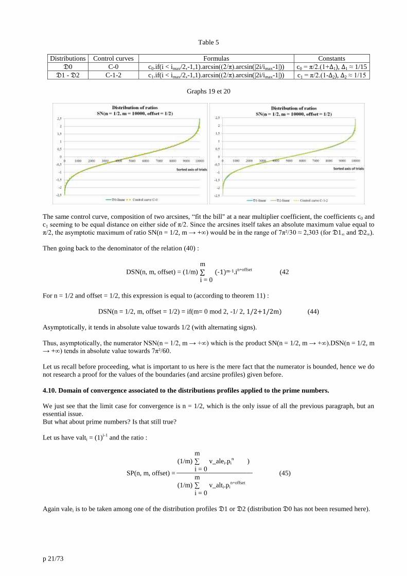
Table 5

Distributions Control curves Formulas Constants

𝔇0 C-0 c0.if(i < imax/2,-1,1).arcsin((2/π).arcsin(|2i/imax-1|)) c0 = π/2.(1+Δ1), Δ1 ≈ 1/15

𝔇1 - 𝔇2 C-1-2 c1.if(i < imax/2,-1,1).arcsin((2/π).arcsin(|2i/imax-1|)) c1 = π/2.(1-Δ2), Δ2 ≈ 1/15

Graphs 19 et 20

The same control curve, composition of two arcsines, “fit the bill" at a near multiplier coefficient, the coefficients c0 and

c1 seeming to be equal distance on either side of π/2. Since the arcsines itself takes an absolute maximum value equal to

π/2, the asymptotic maximum of ratio SN(n = 1/2, m → +∞) would be in the range of 7π²/30 ≈ 2,303 (for 𝔇1∞ and 𝔇2∞).

Then going back to the denominator of the relation (40) :

m

DSN(n, m, offset) = (1/m) ∑ (-1)m-1.in+offset (42

i = 0

For n = 1/2 and offset = 1/2, this expression is equal to (according to theorem 11) :

DSN(n = 1/2, m, offset = 1/2) = if(m= 0 mod 2, -1/ 2, 1/2+1/2m) (44)

Asymptotically, it tends in absolute value towards 1/2 (with alternating signs).

Thus, asymptotically, the numerator NSN(n = 1/2, m → +∞) which is the product SN(n = 1/2, m → +∞).DSN(n = 1/2, m

→ +∞) tends in absolute value towards 7π²/60.

Let us recall before proceeding, what is important to us here is the mere fact that the numerator is bounded, hence we do

not research a proof for the values of the boundaries (and arcsine profiles) given before.

4.10. Domain of convergence associated to the distributions profiles applied to the prime numbers.

We just see that the limit case for convergence is n = 1/2, which is the only issue of all the previous paragraph, but an

essential issue.

But what about prime numbers? Is that still true?

Let us have valti = (1)i-1

and the ratio :

SP(n, m, offset) =

m

(45)

(1/m) ∑ v_alei.pin )

i = 0

m

(1/m) ∑ v_alti.pin+offset

i = 0

Again valei is to be taken among one of the distribution profiles 𝔇1 or 𝔇2 (distribution 𝔇0 has not been resumed here).

p 22/73

Theorem 21 :

The turnaround situation for the 𝔇1∞ and 𝔇2∞ distributions is obtained for offset = 1/2.

Proof

This is the consequence of the near-linear growth of prime numbers.

Indeed, for all i > 1, we define ε(i) = ln(pi)/ln(i)-1. This expression does have meaning for anything i strictly greater than

1. We then get pi = i1+ε(i)

. According to theorem 7, when i increases, the number ε(i) tends towards 0. Indeed, as pi →

i.ln(i) according to the prime numbers theorem, we have in fact ε(i) → ln(ln(p i))/ln(i) and by replacing pi again with a

rough estimate i, we get ε(i) → ln(ln(i))/ln(i). A simple numerical check shows that ln(ln(i))/ln(i) < ε(i) < ln(ln(p i))/ln(i)

for any pi ≥ 7 and that the gap between the upper and lower bound gradually decreases. The terms ε(i) and ln(ln(p i))/ln(i)

are not strictly decreasing, but the term ln(ln(i))/ln(i) does it, and we have ε(i) → ln(ln(i))/ln(i) → 0+ when i → +∞.

We then write the ratio S (n, m → +∞, offset) replacing pi by i1+ε(i)

in the form :

SP(n, m → +∞, offset) =

m

sma(k)+(1/m) ∑ v_alei.in.(1+ε(i))

)

i = k

m

smt(k)+(1/m) ∑ v_alti.i(n+offset).(1+ε(i))

i = k

Let us have SP(n, m, offset) = NSP(n, m)/DSP(n, m, offset).

Let us suppose > 1/2. The numerator of SP(n, m → +∞, offset) diverges and so does the denominator if offset ≥ 1/2

because this is the case when ε(i) = 0. So the terms sma(k) and smt(k) are negligible in front of the terms that follow

them. This can be done for 0 < ε(i) < ε0 where ε0 is arbitrary small. Thus, the ratio SP(n, m → +∞, offset) draws near

the ratio SN(n, m → +∞, offset).

What applies to the first one applies to the other for n > 1/2, especially for the turnaround situation, the offset is equal to

1/2+ε’, where ε’ is arbitrarily small.

The reasoning can be taken again for n < 1/2 considering this time 1/NSP(n, m) and 1/DSP(n, m, offset) and a

turnaround situation 1/2-ε’, where ε’ is arbitrarily small

This means also that the ratio RPN(n, m → +∞, offset) = SP(n, m → +∞, offset)/SN(n, m → +∞, offset) is bounded,

almost surely, when offset = 1/2.

Hence the result.

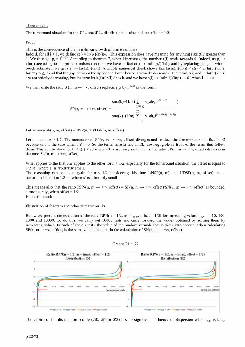
Illustration of theorem and other numeric results

Below we present the evolution of the ratio RPN(n = 1/2, m = imax, offset = 1/2) for increasing values imax == 10, 100,

1000 and 10000. To do this, we carry out 10000 tests and carry forward the values obtained by sorting them by

increasing values. In each of these i tests, the value of the random variable that is taken into account when calculating

SP(n, m → +∞, offset) is the same value taken in i in the calculation of SN(n, m → +∞, offset).

Graphs 21 et 22

The choice of the distribution profile (𝔇0, 𝔇1 or 𝔇2) has no significant influence on dispersion when imax is large

p 23/73

enough (below imax = 10000).

The evolution of these curves is to a horizontal line and a few extreme points with a higher absolute value. The two

curves below are thus the same, only the scale of the ordinate axis has been changed to show the extreme values and the

asymptotic form of the graphic.

Graphs 23 et 24

The results show that the percentage of extreme values decreases with the increase in the imax value. The probability of

such events drops to 0 to infinity and the standard deviation decreases with imax increase as shows as the underneath

table.

Table 6

Standard deviation of distributions

Distributions imax = 10 imax = 100 imax = 1000 imax = 10000

𝔇0 1,3752 0,8487 0,3554 0,3199

𝔇1 2,5218 1,2189 0,3445 0,2746

𝔇2 1,8506 1,2715 0,4171 0,2028

The approximation of the ratio RPN(n = 1/2, m = imax, offset = 1/2) is given by a curve such as α+β.tan(π/2.(2i/imax-1)).

We have, for example for the distributions 𝔇2, α ≈ 0,58 and β ≈ 0.050 for imax = 10, α ≈ 0,44 and β ≈ 0.026 for imax =

100, α ≈ 0,34 and β ≈ 0.013 for imax = 1000, α ≈ 0,30 and β ≈ 0.0085 for imax = 10000. The graph below shows the case

imax = 10000, the other cases adjusting without any difficulty. This is reminiscent of the scattering graphs given in

appendix 2, a typical report marker of two random functions of the same nature. What is important here is that the

coefficient β is outside the term tangent. When β increases asymptotically, which it actually does here, the curve

necessarily approaches the horizontal line and therefore the proportion of extreme values decreases (to 0) when the

choice of imax increases.

Graphs 25

The result on the ratio RPN(n = 1/2, m → +∞, offset = 1/2) being confirmed, we study a few specific points below.

Let us have n = 1/2 and offset = 1/2. The denominator of SP(n, m, offset) is equal to (1/m).(2-3+5-7+11-13+17-

19+….pm). A rough calculation of this expression is not difficult to achieve. We start from the asymptotic approximation

p 24/73

pi+1-pi ≈ ln(pi). So the absolute value |DSP(n, m, offset)| ≈ (2+ln(5)+ln(11)+ln(17)+…+ln(p2ent(m/2)))/m by evaluating

differences of every two terms. Then, |DSP(n, m, offset)| ≈ (1/m).(2+ln(3)+ln(5)+ln(7)+ln(11)+...ln(pm))/2 considering

that two successive prime numbers have similar values. Hence thereafter |DSP(n, m, offset)| ≈ (1/2m).ln(∏pi) <

(1/2m).ln(pmm) = (1/2).ln(pm) → (1/2).pm/m.

As the prime numbers increase, there are necessarily alternating signs and partial compensation compared to the

previous calculation step for sum DSP(n, m, offset). The upper bound serves as an approximate value of the lower bound

sign excepted. The actual calculation shows that in fact DSP(n, m, offset) alternates in sign and approximates

±0,57.ln(pm) for pm = p10000.

So this time DSP(n,m, offset) diverges (while for integers, there was "convergence" with a boundary alternately taking

1/2 and -1/2).

For our argument, however, it is necessary that NSP(n = 1/2, m, offset = 1/2) does not diverge towards infinity when m

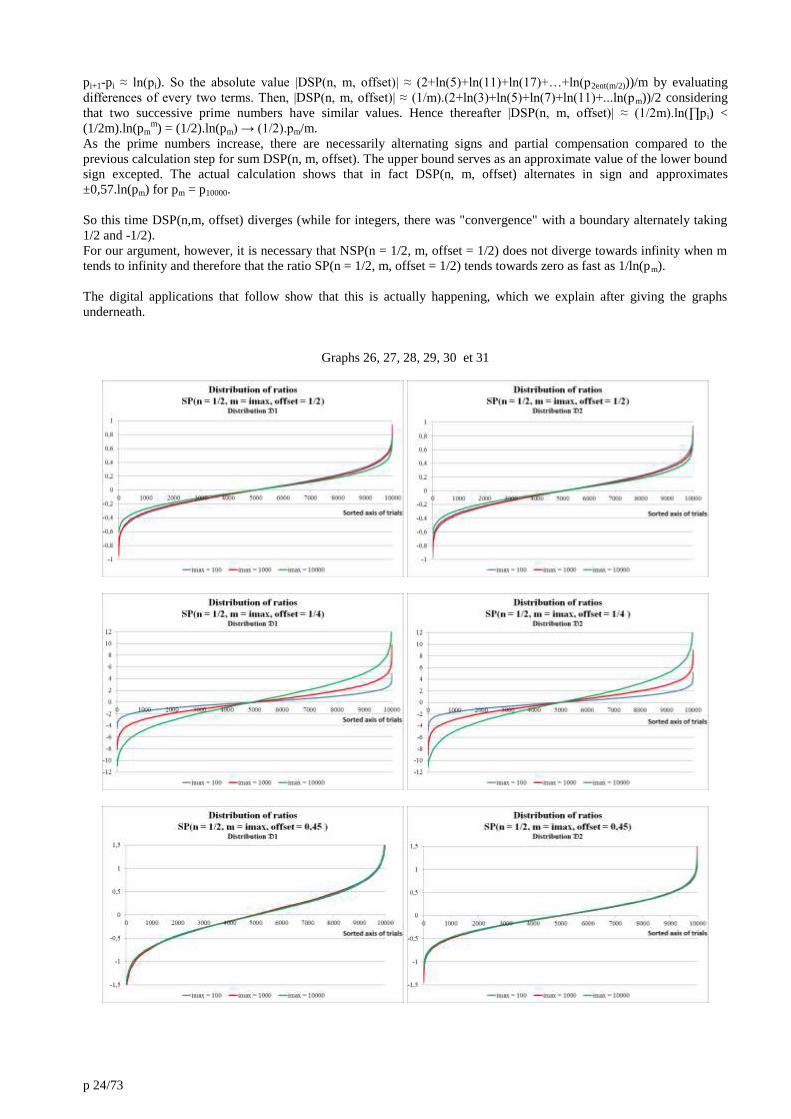
tends to infinity and therefore that the ratio SP(n = 1/2, m, offset = 1/2) tends towards zero as fast as 1/ln(pm).

The digital applications that follow show that this is actually happening, which we explain after giving the graphs

underneath.

Graphs 26, 27, 28, 29, 30 et 31

p 25/73

We see, once again, a turnaround situation between the offset 0,25 and the offset 0,75. Indeed, for the first case (offset

0,25), there is a divergence of the ratio of SP(n, m, offset) when m = imax increases since each graph representative of an

imax choice is further and further away from the x-axis. For the second case (offset 0,75), there is convergence towards

the axis and therefore towards the value 0 since the maximum ordinate value gradually decreases.

For offset 0,5, we observe that the representative curves of ratio SP(n = 1/2, m, offset) approach the axis y = 0 when imax

increases which means asymptotically a value approaching 0 (almost surely). This realizes in the same way for the two

distributions 𝔇1 and 𝔇2, with very similar experimental curves and a turnaround situation for approximate offset 0,45.

We checked, but this is not really necessary here, that 𝔇0 follows the same path.

The ratio SP(n = 1/2, imax = 10000, offset) follows at the level of the turnaround situation, for the offset equal to 0,45

again the same distribution of values observed previously (see Table 5 and graph 20) with control curves composed of

two arcsines.

Table 7

Distributions Control curves Formulas Constants

𝔇1 CP-1 cp1.si(i < imax/2,-1,1).arcsin((2/π).arcsin(|2i/imax-1|)) cp1 ≈ 11/10

𝔇2 CP-2 cp2.si(i < imax/2,-1,1).arcsin((2/π).arcsin(|2i/imax-1|)) cp2 ≈ 8/10

Graph 32

Here again the constants (parameters) are outside the arcsines formulas, the latter being thus pure expressions and thus

somehow the own proof of their veracity.

Only the multiplier coefficient is changing. Moreover, it is different for 𝔇1 and 𝔇2 now, while it was the same in the

example in integers (instead of primes). This is certainly the result of the offset shift from 0,5.

With such curves, the asymptotic maximum expected for ratio SP(n = 1/2, m → +∞, offset0) is therefore in the range of

11π/20 ≈ 1,728 for 𝔇1∞ and 2π/5 ≈ 1,257 for 𝔇2∞, at least bounded ratios.

Hence the previously stated theorem.

Appendix 7 gives the evolution of the NSP(n, m, offset = 1/2) sums from an increasing sorted distribution, gradually

applying the Fisher-Yates algorithm [21] to the said distribution, thus spreading a random weight to each of the i-event

terms.

In these numerical examples, we find the conclusions we have reached previously, including maximums hardly over 1 in

p 26/73

absolute value.

4.11. Predominance of randomness.

The quadratic opposites are part of a given framework, namely distribution profiles 𝔇1∞ et 𝔇2∞. But once this

framework is set, only a random walk seems necessary for the completion of the "events". If the 𝔇0∞ distribution had

been imposed by the elliptical equations, we would have just as well done our deal with this constraint with the same

result.

This is what we would qualify here the predominance of randomness.

5. Theorem de Mertens.

5.1. Riemann series.

Theorem 22 [24]

The convergence radius Re(s) of Riemann's series = Σ 1/ns is 1. There is simple (and absolute) convergence for Re(s) >1

and divergence for Re(α) ≤ 1.

ζ(s) is also called Riemann's Zeta function.

The harmonic series H = ζ(1) diverges like ln(n). Specifically, the term Hn-ln(n) admits a finite limit γ called Euler-

Mascheroni's constant :

γ = lim (1+1/2+1/3+…1/n-ln(n)) ≈ 0,5772156649 (46)

p → +∞

On the convergence radius ]1, +∞[, the Zeta function is equal to its Euler product :

ζ(s) = ∏ 1/(1-p-s)

p ∈ 𝒫

The result is the convergence of ∏p (1-1/ps) on this radius.

Theorem 23

The simple (and absolute) convergence radius of ∏p (1+c/ps), c a constant, is ]1,+∞[ if c ≠ 0 and ]-∞,+∞[ if c = 0.

Proof

Case c = 0 is trivial.

The general proof is similar, but let us suppose in order to simplify that s is a real number greater than 1.

Let us have then c a constant ≠ 0. We have ∏p (1+c/ps) = ζ(s).∏p (1+c/p

s)(1-1/p

s) = ζ(s).∏p (1+(c-1)/p

s-c/p

2s) < ζ(s).∏p

(1+(c-1+ε)/ps) for any ε > 0 since 1/p

2s is asymptotically negligible in front of 1/p

s. Repeating this operation n times, we

get ∏p (1+c/ps) < ζ

n(s).∏p (1+(c-n+n.ε)/p

s). Let us take, for example, ε = 1/2. As c is constant, there is an integer n such as

c-n+n.ε < 0, which leads to ∏p (1+c/ps) < ζ

n(s). If ζ(s) converges, ζ

n(s) converges and thus ∏p (1+c/p

s) also converges.

Formally using ∏p (1+c/ps) = ζ

-1(s).∏p (1+c/p

s)(1-1/p

s)

-1 = ζ

-1(s).∏p (1+c/p

s)(1+1/p

s+c1/p

2s+…) > ζ

-1(s).∏p (1+(c+1-ε)/p

s)

and repeating the operation n times, we can show that if ζ(s) diverges ∏p (1+c/ps) also diverges. The convergence radius

of ∏p (1-1/ps) is therefore that of ∏p (1+c/p

s).

Note : From above, it follows that the convergence radius of ∏p (1+c/ps+c’/p

s’), when Re(s’) > Re(s), is that of ζ(s) and

therefore equals ]1,+∞[, excluding trivial cases c = c’ = 0.

5.2. Mertens third theorem.

Theorem 24

Mertens third theorem [10] gives Euler's product associated with (1-1/p).

We have, γ being the constant of Euler-Mascheroni, the following result (n ≥ 2) :

∏ (1-1/p) = e-γ

/ln(n).(1+O(1/ln(n))) (47)

p ≤ n

The term rounding, not being useful here, we rewrite the theorem in the more manageable simplified form :

p 27/73

∏ (1-1/p) ≡ e-γ

/ln(x) (48) p ≤ x

x → +∞

5.3. Generalization of Mertens’ theorem.

Theorem 25

Let us have a > 1 an integer, then :

∏ (1-a/p) ≡ ca.e-aγ

/lna(x), with ca a constant > 0 (49)

p ≤ x

x → +∞

Proof

Let us have a an integer ≠ 0.

Let us have p an element of the set of prime numbers 𝒫, set that we separate into two parts (the first one possibly

empty): p ≤ a and p > a.

We get, using Newton's binomial formula, the coefficients ci being integers :

(1-1/p)a = 1+c1/p+c2/p

2+…+ca/p

a

We have of course

c1 = -a

Let us write

ma = ∏ (1-1/p)

p ≤ a

We chose ma = 1 if the set ≤ a is empty.

Reminding Mertens’ theorem

∏ (1-1/p) ≡ e-γ

/ln(x) (50) p ≤ x

x → +∞

we then get :

e-aγ

/lna(x) ≡ ∏ (1-1/p)

a . ∏ (1-1/p)

a = ma

a. ∏ (1-a/p+c2/p

2+…+ca/p

a) (51)

p ≤ a

a < p ≤ x

x → +∞

a < p ≤ x

x → +∞

Let us write afterwards (for a < p) :

1-a/p+c2/p2+…+ca/p

a = (1-a/p).(1+(c2/p

2+…+ca/p

a)/(1-a/p))

We get using the first and third terms of relation (51)

∏ (1-a/p) . ∏ (1+(c2/p2+…+ca/p

a)/(1-a/p)) ≡ ma

-a.e

-aγ/ln

a(x)

a < p ≤ x

x → +∞ a < p ≤ x

x → +∞

We have for 1 < a < p, the series expansion 1/(1-a/p) = 1+a/p+m2/p2+m3/p

3+… Then (c2/p

2+…+ca/p

a)/(1-a/p) =

(c2/p2+…+ca/p

a).(1+a/p+m2/p

2+m3/p

3…) = c2/p

2+r2/p

3 + terms of superior orders…

Thus, ∏p→∞ (1+(c2/p2+…+ca/p

a)/(1-a/p)) = ∏p→∞ (1+c2/p

2+r2/p

3+…).

According to theorem 23, this expression converges towards a constant regardless of the value of c2, r2, etc.

We multiply the reverse of this constant by ma-a

and note the new constant so obtained c’a (c’a > 0).

Then :

∏ (1-a/p) ≡ c’a.e-aγ

/lna(x)

(52) a < p ≤ x

x → +∞

For another constant, we have finally :

p 28/73

∏ (1-a/p) ≡ ca.e-aγ

/lna(x)

(53) p ≤ x

x → +∞

Note that this result remains valid for a not an integer (>1), but it is not useful to establish this result here.

We can also write this, c being a constant dependent on a :

∏ (1-a/p)-1

≡ c.lna(x)

(54) p ≤ x

x → +∞

This result is easily verified numerically.

The generalization of Mertens' third theorem allows us to have a relationship between the (constant) coefficient a in

Euler's product and the power assigned to the logarithm.

Of course, for Birch Swinnerton-Dyer's conjecture, the ap coefficient in the ap/p ratio is not a constant, and besides its

value evolves diverging towards infinity (because √p → +∞). However ap/p converges, so it is useful to know more

about this ratio. That is what the following is all about.

6. Arithmetic rank of an elliptic curve.

We introduce a third concept of rank that will join the other two in this article. This rank is called arithmetic since it

comes out from an arithmetic average.

Let us start with its definition.

6.1. Arithmetic average.

Let us have the curve (E) defined by equation y2 = x

3+a.x+b and let us have ap the quadratic opposite for prime number

p. The coefficients a and b are given data.

Definition 10

Let us have M(E,n) the arithmetic average of the error terms api, pi being the i-th prime number, i = 1 to n :

n

M(E,n) = (1/n) ∑ api (55)

i = 1

We call the arithmetic rank rth of the E-curve, the limit, when n tends towards infinity, of the opposite of M(E,n).

rth = lim -M(E,n) (56)

n → +∞

Numeric illustration

Values of the arithmetic rank are illustrated below.

The curves corresponding to these examples are given in appendix 1. In abscissas are carried the algebraic ranks and in

ordinates are the arithmetic ranks calculated from the average coefficients - ap where p is between p1 = 2 and p100000 =

1299709. As the chosen interval is only a small part of the definition domain (which goes to infinity), sometimes

significant differences appear on this figure (representative points in blue, linear trend curve in red).

p 29/73

Graph 33

Appendix 10 provides representative examples of the evolution of this "chaotic" average.

6.2. Link with the Mertens theorem.

We write down fa(i) = api and M = M(E, n → +∞) the average of the quadratic opposite.

Theorem 26

There is a non-zero positive constant f such as f.∏(1-M/pi) is almost surely the best asymptotic approximation of ∏(1-

fa(i)/pi).

Proof

Let us have c some positive constant (c > 0) and let us suppose M ≠ 0.

Let us have R(E,c) the ratio of the following Euler’s products :

∏ (1-fa(i)/pi)

R(E,c) = pi ∈ 𝒫

(57) ∏ (1-c.M/pi)

pi ∈ 𝒫

We have to prove first that c = 1 is the only case where there is no assured divergence of R(E,c) towards infinity or

convergence to 0. The following product deals with prime numbers.

We have R(E,c) = ∏(1-fa(i)/pi).(1-c.M/pi)-1

= ∏pi ≤ p (1-fa(i)/pi).(1-c.M/pi)-1

∏ pi > p (1-fa(i)/pi).(1-c.M/pi)-1

. We choose p

such as the absolute value |rvi| = |c.M/pi| < 1 for any pi > p. Such a p always exists since M is bounded (and constant), c

is constant and pi diverges towards infinity. We write rp = ∏pi ≤ p (1-fa(i)/pi).(1-c.M/pi)-1

(which is therefore simply a

constant). We have R(E,c) = rp. ∏ pi > p (1-fa(i)/pi).(1-c.M/pi)-1

= rp ∏ pi > p (1-fa(i)/pi).(1+(c.M/pi)1+(c.M/pi)

2+

(c.M/pi)3+...). We develop two by two the terms that have the same powers for pi. We get R(E,c) = rp.∏ pi > p (1-

(fa(i)/pi)+(c.M/pi)1-(fa(i)/pi).(c.M/pi)

1+(c.M/pi)

2-(fa(i)/pi).(c.M/pi)

2+(c.M/pi)

3+...). As rvi is bounded by 1, we get

1+(c.M/pi)1+ (c.M/pi)

2+(c.M/pi)

3+... = 1/(1-c.M/pi) as a geometric sum. It thus follows R(E,c) = rp.∏ pi > p (1-(c.M-

fa(i))/(pi.(1-c.M/pi))) = rp.∏ pi > p (1-(c.M-fa(i))/(pi-c.M)) = rp.∏ pi > p 1-(c.M-fa(i))/qi where qi = pi-c.M = pi.(1-rvi) and rvi

→ 0. Hence R(E,c) = rp.∏ pi > p 1-(c.M-fa(i))/qi. = rp.∏ pi > p (1-(c-1).M/qi-(M-fa(i))/qi) and then R(E,c) = rp.∏ pi > p ((1-(c-

1).M/qi)(1-(M-fa(i))/qi)+(c-1).M.(M-fa(i))/qi2).

According to theorem 23, the convergence radius of ∏p (1+c/ps) is 1. The term fa(i) is within the Hasse interval ]-2.pi

1/2,

2pi1/2

[ and M is a constant. The ratio (c-1).M.(M-fa(i))/qi2 is therefore equivalent to a term in c’/pi

3/2 and ∏ pi > p (1+(c-

1).M.(M-fa(i))/qi2) therefore converges asymptotically. This term will therefore intervene, in the R(E,c) ratio, by a

constant multiplier contribution c’’, that is R(E,c) = rp.c’’.∏ pi > p (1-(c-1).M/qi).(1-(M-fa(i))/qi) = rp.c’’.∏ pi > p (1-(c-

1).M/qi).∏ pi > p (1-(M-fa(i))/qi).

Let us look at the three cases c > 1, c < 1 and c = 1.

If c > 1, such as M < 0, the term ∏ pi > p (1-(c-1).M/qi) diverges, according to theorem 25, like ln(c-1).(-M)

(pi), the difference

between pi and qi being marginal at infinity, and so regardless of the precise behaviour (convergence or divergence) of ∏

pi > p (1-(M-fa(i))/qi), the global term R(E,c) diverges.

If c < 1, as M < 0, the term ∏ pi > p (1-(c-1).M/qi) converges to 0, according to theorem 25 again, like the expression 1/ln(1-

c).(-M)(pi), the difference between pi and qi being still marginal at infinity, and regardless of the precise behaviour of ∏ pi >

p 30/73

p (1-(M-fa(i))/qi), the global term R(E,c) converges to 0.

Let us have f a continuous function such as f(i) = fa(i) for all integers and let us join the values f(i) by linearly pieces.

Such a function necessarily exists. Through the theorem of intermediate values, the product R(E,c) goes from infinity to

0 at c = 1. If some c value is appropriate to give the asymptotic behaviour of the expression ∏(1-fa(i)/pi), then it can only

be c = 1.

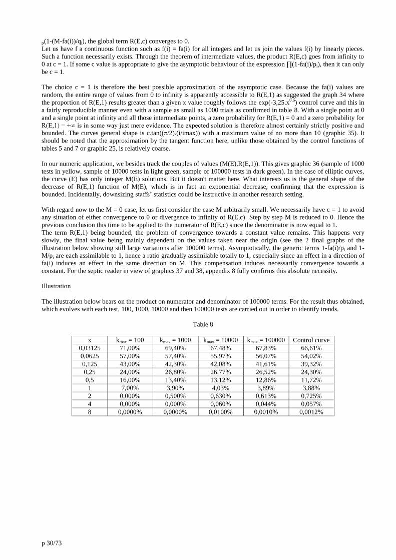
The choice c = 1 is therefore the best possible approximation of the asymptotic case. Because the fa(i) values are

random, the entire range of values from 0 to infinity is apparently accessible to R(E,1) as suggested the graph 34 where

the proportion of R(E,1) results greater than a given x value roughly follows the exp(-3,25.x0,6

) control curve and this in

a fairly reproducible manner even with a sample as small as 1000 trials as confirmed in table 8. With a single point at 0

and a single point at infinity and all those intermediate points, a zero probability for R(E,1) = 0 and a zero probability for

R(E,1) = +∞ is in some way just mere evidence. The expected solution is therefore almost certainly strictly positive and

bounded. The curves general shape is c.tan((π/2).(i/imax)) with a maximum value of no more than 10 (graphic 35). It

should be noted that the approximation by the tangent function here, unlike those obtained by the control functions of

tables 5 and 7 or graphic 25, is relatively coarse.

In our numeric application, we besides track the couples of values (M(E),R(E,1)). This gives graphic 36 (sample of 1000

tests in yellow, sample of 10000 tests in light green, sample of 100000 tests in dark green). In the case of elliptic curves,

the curve (E) has only integer M(E) solutions. But it doesn't matter here. What interests us is the general shape of the

decrease of R(E,1) function of M(E), which is in fact an exponential decrease, confirming that the expression is

bounded. Incidentally, downsizing staffs’ statistics could be instructive in another research setting.

With regard now to the M = 0 case, let us first consider the case M arbitrarily small. We necessarily have c = 1 to avoid

any situation of either convergence to 0 or divergence to infinity of R(E,c). Step by step M is reduced to 0. Hence the

previous conclusion this time to be applied to the numerator of R(E,c) since the denominator is now equal to 1.

The term R(E,1) being bounded, the problem of convergence towards a constant value remains. This happens very

slowly, the final value being mainly dependent on the values taken near the origin (see the 2 final graphs of the

illustration below showing still large variations after 100000 terms). Asymptotically, the generic terms 1-fa(i)/pi and 1-

M/pi are each assimilable to 1, hence a ratio gradually assimilable totally to 1, especially since an effect in a direction of

fa(i) induces an effect in the same direction on M. This compensation induces necessarily convergence towards a

constant. For the septic reader in view of graphics 37 and 38, appendix 8 fully confirms this absolute necessity.

Illustration

The illustration below bears on the product on numerator and denominator of 100000 terms. For the result thus obtained,

which evolves with each test, 100, 1000, 10000 and then 100000 tests are carried out in order to identify trends.

Table 8

x kmax = 100 kmax = 1000 kmax = 10000 kmax = 100000 Control curve

0,03125 71,00% 69,40% 67,48% 67,83% 66,61%

0,0625 57,00% 57,40% 55,97% 56,07% 54,02%

0,125 43,00% 42,30% 42,08% 41,61% 39,32%

0,25 24,00% 26,80% 26,77% 26,52% 24,30%

0,5 16,00% 13,40% 13,12% 12,86% 11,72%

1 7,00% 3,90% 4,03% 3,89% 3,88%

2 0,000% 0,500% 0,630% 0,613% 0,725%

4 0,000% 0,000% 0,060% 0,044% 0,057%

8 0,0000% 0,0000% 0,0100% 0,0010% 0,0012%

p 31/73

Graphics 34, 35 and 36

Graphics 37 and 38

Typical evolutions of R(E,1) function of i the indice of pi.

6.3. Equality of arithmetic and analytical rank.

Theorem 27

The arithmetic rank ath and the analytical rank ran are identical.

Proof

Let us have rth the opposite of the asymptotic average of the error terms ap.

According to theorem 26, we have :

∏ (1-ap/p) ≈ C/lnrth

(x) when x→ +∞ (58)

p≤ x

On the other side, according to theorem 4, if ∏p≤ x (1-ap/p) ∼ C.lnr(x) when x→ +∞, then L(E,s) ∼ C’.(s-1)

r when s → 1.

The latter being the analytical rank ran, it is thus equal to rth. Arithmetic rank and analytical rank, when they exist, can

only be equal.

p 32/73

7. Distributions relative to the quadratic opposite.

7.1. Situation analysis.

According to Hasse's theorem, the ratios ap/(2p1/2

) are all in range ]-1,1[ and can therefore be written in the form cos(θp).

To study cos(θp) values, the values reached for a p = 2 to pi sample, i infinity-oriented, are sorted in increasing values

and distribution profiles are examined.

Theorem 28

For elliptical curves, there are two limit distributions 𝔇1∞ et 𝔇2∞ of the values cos(θp), one corresponding to complex

multiplication curves and the other corresponding to curves without complex multiplication.

References of the proof

The distribution 𝔇1∞ for which E has a complex multiplication is based on Hecke's work and derives from an

equidistribution on the unit circle (see reference [5]). This point is therefore settled.

The conjecture of Mikio Satō and John Tate is interested in the distribution 𝔇2∞ for which E has no complex

multiplication. It predicts that the measure of probability of θp is (2/𝜋).sin2(θp).dθp in the interval [0,π] (see reference

[26]). At the limit pi → +∞, we have Richard Taylor and Michael Harris theorem in collaboration with Laurent Clozel,

Nick Shepherd-Barron (2006), T. Barnet-Lamb and D. Geraghty (2019) on the local and global representations of Galois

[2][5]. This point has therefore been settled recently as well.

Note :

The concept generalizes to other curves (including genres ≠ 1, cf. [13]).

7.2. Numeric illustration.

The selected examples are represented for a sample p1 = 2 to p100000 = 1299709. Digital representations necessarily show

discrepancies to the theoretical distributions. We chose as “control curves” two curves of algebraic rank 0, one for

complex multiplication (CM) examples, the other for curves that lack it (CW). For higher-ranked curves, representations

are increasingly obviating from the "ideal." However, asymptotically, there are only two limit forms, regardless of the

rank of the chosen curve.

Table 9

Ref. Complex

multiplication

Coefficients

[a1, a2, a3, a4, a6]

Average(-ap)

p ≤ pimax = p100000

C0m Yes [0, 0, 0, 0, 1] -0,455

C0w No [0, -1, 1, 0, 0] -0,312

Graph 39

Type 1 : Sorted distribution of cos(θp) in presence of complex multiplication

p 33/73

Graphs 40

Type 2 : Sorted distribution of cos(θp) in the absence of complex multiplication

For the two control examples (of algebraic rank 0), the deviation from the theoretical curves is not visible. There is a

perfect superposition.

7.3. Explicit formulas.

We chose to give distribution relationships explicitly and not as a probability measure in order to undertake additional

calculations of deviations also in non-asymptotic situations.

Let us write x = i/imax, so that x varies in interval [0,1].

We get :

Table 10

Complex

multiplication cos(θpi)

Reminder

distributions

Yes

if(and(x ≥ 1/4, x ≤ 3/4), 0, 1).

if(x ≥ 1/2, 1, -1).

sine(π/2.(1-4x))

𝔇1∞

No

cos(π.(f

-1(x)-1))

where 0 ≤ x ≤ 1

f(u) = u-sine(2π.u)/2π 𝔇2∞

Elaboration of the explicit expression of Satō-Tate distribution.

Let us have pi a prime number and corresponding error term api = 2√pi.cos(θpi) and error angle θpi. The Satō-Tate

distribution gives the asymptotic proportion of indexes i that have an angle around the given value θ.. This proportion is,

between i and i+di, the limit quantity di = (2/𝜋).sin2(θ).dθ, with θ varying in the interval [0,π]. Over this interval, we get

of course

2/π. ∫ sin²(θ). dθ𝜋

0 = 1 (59)

which is easily verified by using cos(2z) = cos²(z)-sin²(z) = 1-2sin²(z), and then sin²(z) = (1-cos(2z))/2.

Using the same expression, we also get the cumulative proportion, between 0 and θ,

%i = (1/π).(θ-sin(2θ))/2 (60)

Let us write θ = π.u in order to get u is in the interval [0,1] and let us note the cumulative proportion v = %i.

That gives for axes (u,v) both limited by [0,1] :

v = f(u) = u-sin(2π.u)/2π (61)

The derivative f ’(u) is equal to 1-cos(2π.u) and therefore positive or null. It is null for u = 0 and u = 1 and maximum

and equal to 1 for u = 1/2. The function f is strictly increasing from 0 to 1 in the interval [0,1].

The function f

-1, reciprocal function of f, is defined by simple permutation of u and v axes. This function is therefore

also strictly increasing from 0 to 1 in the interval [0,1]. Its derivative in the renamed axes (x,y) is equal to +∞ at x = 0

p 34/73

and x = 1 and equal to 1 at x = 1/2.

The x-axis then represents the proportion of i's at some reduced angle y = θ/π. To get back the data of the 𝔇2

distribution in table 10, it is necessary and sufficient to use :

θ/π = f

-1(x) (62)

That is also

cos(θ) = cos(π.f

-1(x)) (63)

As this function is decreasing from 1 to -1 and the representation adopted is increasing, the following correction is

necessary :

cos(θ) = cos(π.(f

-1(x)-1)) (64)

For numeric applications, the use of a non-explicit reciprocal function is of little practice. We have also replaced the

function cos(π.(f

-1(x)-1)) with the substitution function, and approximation of very good quality, which follows :

if(x < 1/2, -1, 1).cos(arcsin(c.[(1-x).x]ln(c)/ln(4)

) (65)

It can also be written if(x < 1/2, -1, 1).(1-c².((1-x).x)ln(c)/ln(2)

)1/2

) as well as if(x < 1/2, -1, 1).(1-

(sin(2.arcsin√x))2.ln(c)/ln(2)

)1/2

using sin²(z)+cos²(z) = 1 and sin(2z) = 2.sin(z).cos(z).

The reader will find in appendix 9 comparative data.

Theorem 29

The limit distributions are symmetrical to the middle point (which we can call origin point).

Proof

This is the case with non-asymptotic relationships and this is therefore true asymptotically.

7.4. Spread at the two limit distributions.

Proposition 1

The maximum relative deviation dev/imax of distributions to the two asymptotic distributions is proportional to the

arithmetic rank of E.

Argument

For the calculation regarding the distribution 𝔇2 (without complex multiplication CW), we use the substitution function.

The distribution thus obtained for a sample of prime numbers up to pi is written 𝔇1pi or 𝔇2pi depending on the case.

We have api = 2.pi1/2

.cos(θpi).

Let us imagine that the deviation, compared to the curve corresponding to rank 0, propagates in an equiprobable way to

each instance i. Let us look at the result on the distribution curves in a number of points :

- case 1 : at i = imax/4 and i = 3.imax/4 for the distribution 𝔇1pi - case 2 : at i = imax/2 for the distribution 𝔇2pi.

For the first case, the effect of switching from api-0 to api-r allows us to write at i = 3imax/4 (for example), the

approximate equality :

2.p3.imax/41/2

.sin(π/2.(1-4(3.imax/4)/imax))-0

≈

2.p3.imax/4+dev1/2

.sin(π/2.(1-4(3.imax/4+dev)/imax))-r

where dev is the deviation of the intersection point of the cos(θpi) distribution curve with the abscissa axis near 3.imax/4.

The first term is null because we chose rank 0.

We get :

r ≈ 2.p3.imax/4+dev1/2

.sin(π/2.(1-4(3.imax/4+dev)/imax))

≈ 2.p3.imax/4+dev1/2

.sin(π/2.(1-3-4.dev/imax))

≈ 2.p3.imax/4+dev1/2

.sin(2π.dev/imax)

Let us suppose dev/imax << 1 in first approximation.

We get applying sin(ε) ≈ ε, r ≈ 4π.p3.imax/4+dev1/2

.dev/imax. By using in addition p3.imax/4+dev ≈ p3.imax/4, we get the

expression of the deviation reported to the sample size dev/imax ≈ (1/4π).p3.imax/4-1/2

.r.

p 35/73

However, one must recall here that half of the sample of the api is "forced" to 0, so the deferral of the deviation is only on

the other half and thus doubles this one. The corrected expression is therefore :

dev ≈

1 r (66)

imax 2π.(p3.imax/4)1/2

A similar calculation gives, at imax/4, the following corrected expression :

dev ≈

1 r (67)

imax 2π.(pimax/4)1/2

The relative deviation is thus proportional to the arithmetic rank of E (at constant imax).

For the second case, the substitution formula for the distribution 𝔇2pi is written approximately using cos(arcsin(t)) = (1-

t2)

1/2, 0 ≤ t ≤ 1 :

cos(θpi→∞) = lim imax→∞ if(i < imax/2, -1, 1).[1-c2.((1-i/imax).(i/imax))

ln(c)/ln(2)]

1/2 (68)

The effect of switching from api-0 to api-r allows us to write also at i = imax/2, the approximate equality :

2.pimax/21/2

.(1-c2.((1-(imax/2)/imax).((imax/2)/imax))

ln(c)/ln(2))

1/2-0

≈

2.pimax/2+dev1/2

.(1-c2.((1-(imax/2+dev)/imax).((imax/2+dev)/imax))

ln(c)/ln(2))

1/2-r

where dev is the deviation of the intersection point of the cos(θpi) distribution curve with the abscissa axis near imax/2.

The first term is again equal to zero.

We get :

r ≈ 2.pimax/2+dev1/2

.(1-c2.((1-(imax/2+dev)/imax).((imax/2+dev)/imax))

ln(c)/ln(2))

1/2

≈ 2.pimax/2+dev1/2

.(1-c2.((1/2-dev/imax).(1/2+dev/imax))

ln(c)/ln(2))

1/2

≈ 2.pimax/2+dev1/2

.(1-c2.(1/4-(dev/imax)

2)

ln(c)/ln(2))

1/2

≈ 2.pimax/2+dev1/2

.(1-(1-(2.dev/imax)2)

ln(c)/ln(2))

1/2

Let us suppose dev/imax << 1 at first approximation.

It follows applying (1-ε)α ≈ 1-α.ε, r ≈ 2.pimax/2+dev

1/2.(ln(c)/ln(2))

1/2.(2.dev/imax).

Hence, using in addition pimax/2+dev ≈ pimax/2, the expression of the deviation related to sample size :

dev ≈

(ln(2)/ln(c))1/2

r (69)

imax 4.(pimax/2)1/2

The relative deviation is proportional, with constant imax, to the arithmetic rank of E.

Let us note that 1/2π ≈ 0,15915 et (ln(2)/ln(c))1/2

/4 ≈ 0,31625.

With the choice imax = 100000, we get √pimax/2 ≈ 782,274, √pimax/4 ≈ 535,833, √p3imax/4 ≈ 975,275, hence the approximate

deviation dev/r ≈ 29,70 at imax/4 and dev/r ≈ 16,32 at 3.imax/4 with complex multiplication and dev/r ≈ 39,594

without complex multiplication.

The numerical results for our curve sample are as follows.

p 36/73

With complex multiplication

Curves Average rarith

p ≤ p100000

Awaited

deviation

Observed

deviation Ratio

C0m -0,455 imax/4 -14 -70 5,2

3.imax/4 -7 -40 5,4

C1m 0,653 imax/4 19 125 6,4

3.imax/4 11 20 1,9

C2m 1,328 imax/4 39 -35 -0,9

3.imax/4 22 175 8,1

C3m 3,915 imax/4 116 220 1,9

3.imax/4 64 270 4,2

C4m 5,394 imax/4 160 240 1,5

3.imax/4 88 290 3,3

C5m 4,860 imax/4 144 340 2,4

3.imax/4 79 380 4,8

Average 3,7

Without complex multiplication

Curves Average rarith

p ≤ p100000

Awaited

deviation

Observed

deviation Ratio

C0w -0,312 -12 -150 (12,1)

C1w 1,472 58 0 0,0

C2w 2,537 100 320 3,2

C3w 4,39 174 430 2,5

C4w 3,039 120 330 2,7

C5w 4,87 193 480 2,5

C6w 6,549 259 340 1,3

C7w 7,406 293 750 2,6

C8w 6,532 259 530 2,0

C9w 7,395 293 650 2,2

C10w 10,754 426 900 2,1

C11w (a) 14,463 573 990 1,7

C11w (b) 11,354 450 910 2,0

C12w 11,784 467 1050 2,3

C13w (a) 6,963 276 790 2,9

C13w (b) 11,574 458 780 1,7

C14w 13,643 540 1260 2,3

C15w 16 634 1050 1,7

C16w (a) 19,375 767 1530 2,0

C16w (b) 17,039 675 1250 1,9

C17w 18,135 718 1470 2,0

C18w 16,95 671 1480 2,2

C19w 18,972 751 1450 1,9

C20w 19,164 759 1650 2,2

C22w 25,129 995 1970 2,0

C24w 26,098 1033 1960 1,9

C27w 26,958 1067 2060 1,9

C28w 24,434 967 2010 2,1

Average 2,1

On average, in the case of complex multiplication, the actual deviation is 4 times greater than that awaited while,

without complex multiplication, the ratio is in the order of 2 times.

It is obvious that there can be no deviation from the extreme values -1 and 1 of cos(θpi). We can expect a gradual, not

necessarily linear, distribution of the gap from the values where cos(θpi) = 0 up to these ends.

In fact, the deviations observed will be at maximum at the selected coordinates. Obtaining a double value (the ratio 4

remains strong here but based on few examples) compared to an expected average on the entire sample p0 to pimax is

therefore not surprising to these abscissas.

For such a distribution, the relative deviation dev/imax would be written in the following form, assuming, for example, a

linear profile

p 37/73

dev ≈

devuniform .if(CM true, 4, 2).if(i ≥ imax/2, i/imax, (imax-i)/imax) (70)

imax imax

or assuming, for example, a sine profile

dev ≈

devuniform .if(CM true, 4, 2).(4/π).sin(π.i/imax) (71)

imax imax

and is still proportional to r through the initial expression.

Illustration

Appendix 11 provides representative examples of deviations for the two cases of distributions for imax = 100000.

Theorem 30

There are only two distinct asymptotic distributions.

Proof

Let us return to the expressions obtained previously, on the one hand for the curves of complex multiplication, namely

relationships (66) and (67) and on the other hand without complex multiplication, namely the relationship (68). For all

three, the proportionality factor in front of r is in the order of magnitude of (1/pimax)1/2

and therefore tends towards 0

when imax → +∞. So the relative deviation tends towards 0 to infinity.

This is totally expected since ap = 2√p.cos(θ) imposes ap+r = 2√p.cos(θ+ε), for a ε all the smaller as p is larger.

Graphs 60 and 61 are an illustration in appendix 11 of this asymptotic merger.

8. Impact of copies of ℤ.

8.1. Recovering by error terms.

Lemma 1

Let us have P1 = (x1,y1), P2 = (x2,y2), …, Pi = (xi,yi) distinct solutions in ℚ of the elliptical equation E. So the probability

of having non-distinct solutions in the finite field Fp of the equation E tends towards 0 when p tends towards infinity.

Proof

As the points P1, P2, …, Pi are distinct, a modulo p equality is fortuitous. The first choice of a point being made (for

example P1), the equality between a coordinate (for example the abscissa) of P1 and a coordinate P2 is avoided p-1 times,

then the equality between a coordinate of P3 and those of (P1 and P2) is avoided p-2 times, and so on. So we have in

principle at least (p-1).(p-2)...(p-i-1) cases on a total of pi-1

where a duplicate is avoided. For a point to be confused with

itself, both the abscissa xi and the ordinate yi must be the same. This means that the "i distinct points" event has at least a

proportion of cases equal to ((p-1).(p-2)….(p-i+1)/pi-1

)2. The proportion of cases for which at least one point is not

distinct from another is then equal, modulo p, to 1-((p-1).(p-2)….(p-i+1)/pi-1

)2. This term is lower than ((i-1)!/p

i-1)

2. For

given i, this term naturally tends towards 0 when p tends towards infinity. Hence the result.

Note

The effect on ap is "easily" explained from this lemma.

Let us have E an elliptic curve of rank 1. Let us have P1, P2, …, P∞ its solution points on E(ℚ). These are free solutions

"imposed" by a bias originating in the choice of coefficients values [a1, a2, a3, a4, a6] of the equation of the elliptic curve.

We then build an injection between each Pi and an additional solution imposed in #E(𝔽p) for each p by making a

projection i ∈ ℕ to p ∈ 𝒫 :

Pi → <Pi mod p> (72)

Each projection locally increases the number of solutions #E(𝔽p) by a unit, which reduces ap by one unit.

However, this assertion is not an inevitable result. It cannot be issued without precaution. Indeed, there is no absolute

necessity that the so-called "free" solution will actually be added to existing ones. It could very well simply intervene in

the place of the "already existing" one and therefore do not change anything at all. Therefore, we need an additional

argument here that demonstrates the real existence of this addition which we are undertaking now.

p 38/73

8.2. Calibration of the reciprocal effect of a Z copy and of rank 1.

Theorem 31

The analytic rank of the cancellation of L(E,s) at s = 1 is equal to 0 if and only if the corresponding elliptic curve does

not have infinite order points on ℚ.

Theorem 32

The analytic rank of the cancellation of L(E,s) at s = 1 is equal to 1 if and only if the corresponding elliptic curve has 1

infinite order points on ℚ.

Reference of the proof of the two theorems

The proof is due to Victor Kolyvagin, Benedict Gross and Don Zagier [28].

In 1983, Benedict Gross and Don Zagier showed that if a modular elliptic curve has a zero of order 1 at s = 1 then it has

a rational point of infinite order. In 1990, Victor Kolyvagin showed that a modular elliptic curve E for which L(E,1) is

not equal to zero is of rank 0 and a modular elliptical curve E for which L(E,1) has a zero of order 1 at s = 1 is of rank 1.

Hence the following statement :

Theorem 33

There is an equivalence between the absence of a copy of Z and the average of the term error, namely the arithmetic

rank, is equal to 0.

E(ℚ) ≃ ℤ0 ⊕ E(ℚ)

tors ⇔ rth = 0 (73)

In addition, the reduced error terms ap/√p evolve as a pseudo-random variable vi (without bias) when rth = 0 with the

distribution profile 𝔇1∞ or 𝔇2∞.

Proof

According to theorem 31, the absence of a copy of Z implies here that the algebraic rank ral is equal to 0. Then, the

equality of the analytical and arithmetic ranks derives from the theorem 27, thus rth = 0.

In addition, theorem 28 completes the proof.

Theorem 34

There is an equivalence between the existence of 1 copy of Z and the average of the term error, namely the arithmetic

rank, is equal to 1.

E(ℚ) ≃ ℤ1 ⊕ E(ℚ)

tors ⇔ rth = 1 (74)

In addition, the reduced errors terms ap/√p evolve as a pseudo-random variable with an average bias rth = 1.

Proof

This is the repeat of the proof of theorem 33.

8.3. Generalization to ℤn and rank n.

Theorem 35

There is equivalence between the existence of n copies of Z and the average of the term error, namely the arithmetic

rank, equal to n.

E(ℚ) ≃ ℤn ⊕ E(ℚ)

tors ⇔ rth = n (75)

Proof

This stems from the calibration of the arithmetic rank which shows the effect of one copy of Z. It provides an average

bias of 1 to rth. Each additional copy gives an additional bias of 1 to rth. In effect, for small pi values, two distinct points

can give the same modulo pi point, but asymptotically according to lemma 1, the probability of such an event tends

towards 0. The asymptotic probability of no overlapping of n points, n given in advance, is 1 and the proportion of

asymptotic numbers pi is 100% compared to "small" pi values (ε/∞ = 0%). as there are an infinity of prime numbers.

Each bias of a unit is therefore statistically transferred in its entirety. Hence the result.

p 39/73

Illustration

The curves in appendix 10 show the evolution of the mean value, function of pi, for the example listed in appendix 1. We

give below the calculation taken much further for the curve of rank 28 found by Noam Elkies. The calculation is done

systematically, but the values statement for the graph is extracted only every 10000 steps (the last point recorded

corresponds to i = 105090000).

This curve shows that the expected order of magnitude is matched and that the copies of Z are "registered" in the

average of the quadratic opposite.

Graphic 41

Theorem 36

There is equivalence between the existence of n copies of Z and the analytical rank equal to n.

E(ℚ) ≃ ℤn ⊕ E(ℚ)

tors ⇔ r = n (76)

Proof

This stems then, the previous point validated, from Mertens's theorem because rth = n ⇒ r = n.

9. Conclusion.

The study in this article confirms Birch and Swinnerton-Dyer's conjecture.

This result, it seems to us, is however without real help.

Indeed, the implementation of the proof is based on the average of the quadratic opposite. However, the previous

illustation shows that the average of the error terms undergo very large deviations from the asymptotic expected value

and this even for a numeric search pushed relatively far corresponding to half a day of calculation with the Pari GP tool.

The minimum and maximum thus obtained (for a step for i of 100000), in the case of the elliptic curve of raank 28 and

in the domain investigated here, show a gap equal to approximately 17/2. Without prior knowledge of the effective rank

of the curve, the use of this type of numeric results is therefore far from providing an accurate assessment.

If the erratic behaviour api could be exploited in relative value for a very high rank, it is totally inappropriate for lesser

ranks. The table below summarises the uncertainty about the measurement (given by max-min) that renders the

calculation unusable on the usual ranks’ range:

Table 11

Curve reference C4w C12w C28w

Rank 4 12 28

Research range pi < 1E+10 1E+9 2E+9

Min -0,3784 6,3458 20,7741

Max 8,0911 14,8806 29,3654

Max-Min 8,4695 8,5348 8,5913

p 40/73

Graphics 42 and 43

The background noise of the measurement is in the order of magnitude of a decade when the maximum conceivable

deviation is half a unit for a pausible numerical assessment. It seems here that the calculation must be extended by a 100

times factor or even more.

It is therefore still indispensable for us to know the list of rational generators of each copy of Z in order to conclude

anything about the value of the rank.

p 41/73

10. References.

[1] https://www.claymath.org/sites/default/files/birchswin.pdf

[2] https://www.claymath.org/people/richard-taylor

[3] Christophe Breuil, Brian Conrad, Fred Diamond et Richard Taylor. On the modularity of elliptic curves

over Q. JAMS, vol. 14, n° 4, 2001, p. 843-939.

https://fr.wikipedia.org/wiki/Theorem_de_modularité

[4] Andries E. Brouwer. Modell Theorem. https://www.win.tue.nl/~aeb/2WF02/mordell.pdf

[5] Henri Carayol. Séminaire Bourbaki. 59ème

année . 2006-2007. n°977. La conjecture de Satō-Tate d’après

Clozel, Harris, Sherherd-Barron, Taylor. Henri Carayol. Page 977-01.

[6] J. E. Cremona. University of Warwick, U.K. Elliptic Curve Data.

https://johncremona.github.io/ecdata/

[7] Andrej Dujella. High rank elliptic curves with prescribed torsion.

https://web.math.pmf.unizg.hr/~duje/tors/tors.html

[8] Dorian M. Goldfeld. 1982. Sur les produits partiels eulériens attachés aux courbes elliptiques . C.R. Acad.

Sciences Paris Série I Math 294 : 471-474.

[9] Alain Kraus. Université Pierre et Marie Curie. Cours de cryptographie MM067-2009/10.

https://www.math.univ-paris13.fr/~boyer/enseignement/crypto/Chap7.pdf

[10] Frantz Mertens. Ein Beitrag zur analytischen Zahlentheorie. Journal fûr die reine und angewandte

Mathematik. Vol. 78, 1874, p. 46-62 (Journal de Crelle)

[11] J.S. Milne. Elliptic curves. 2006.

https://www.jmilne.org/math/Books/ectext6.pdf

[12] A. Silverberg. Groups order formulas for reductions on CM elliptic curves. 2010.

http://www.math.uci.edu/~asilverb/bibliography/silverbergagct.pdf

[13] Andrew V. Sutherland. Satō-Tate distributions.

https://math.mit.edu/~drew/.

https://arxiv.org/pdf/1604.01256.pdf

[14] Gérald Tenenbaum. Introduction à la théorie analytique et probabiliste des nombres. Belin. 2008.

[15] Gérard Villemin. http://villemin.gerard.free.fr/Wwwgvmm/Identite/Somme.htm

[16] Michel Volle. http://www.volle.com/travaux/calcul.pdf

Blaise Pascal (1623-1662) dans le traité Potestatum Numericarum Summa

[17] https://fr.wikipedia.org/wiki/Variable_aléatoire

[18] https://fr.wikipedia.org/wiki/Estimateur_(statistique)

[19] https://fr.wikipedia.org/wiki/Loi_uniforme_continue

[20] https://fr.wikipedia.org/wiki/Loi_de_Bates

[21] https://fr.wikipedia.org/wiki/Mélange_de_Fisher-Yates

[22] https://fr.wikipedia.org/wiki/Série_alternée

[23] https://fr.wikipedia.org/wiki/Equation_de_Weierstrass

[24] https://fr.wikipedia.org/wiki/Fonction_zéta_de_Riemann

[25] https://fr.wikipedia.org/wiki/Série_de_Dirichlet

[26] https://en.wikipedia.org/wiki/Sato-Tate_conjecture.

[27] https://fr.wikipedia.org/wiki/Theorem_de_Hasse

[28] https://fr.wikipedia.org/wiki/Conjecture_de_Birch_et_Swinnerton-Dyer

[29] https://forums.futura-sciences.com/mathematiques-superieur/371786-somme-racines-carrees-premiers-

entiers.html

[30] https://hubertschaetzel.wixsite.com/website

http://sites.google.com/site/schaetzelhubertdiophantien/

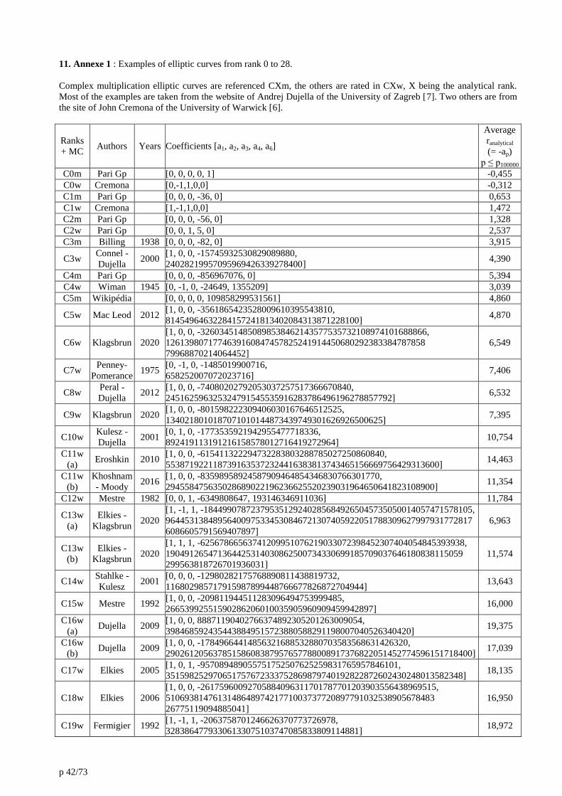
p 42/73

11. Annexe 1 : Examples of elliptic curves from rank 0 to 28.

Complex multiplication elliptic curves are referenced CXm, the others are rated in CXw, X being the analytical rank.

Most of the examples are taken from the website of Andrej Dujella of the University of Zagreb [7]. Two others are from

the site of John Cremona of the University of Warwick [6].

Ranks

+ MC Authors Years Coefficients [a1, a2, a3, a4, a6]

Average

ranalytical

(= -ap)

p ≤ p100000

C0m Pari Gp [0, 0, 0, 0, 1] -0,455

C0w Cremona [0,-1,1,0,0] -0,312

C1m Pari Gp [0, 0, 0, -36, 0] 0,653

C1w Cremona [1,-1,1,0,0] 1,472

C2m Pari Gp [0, 0, 0, -56, 0] 1,328

C2w Pari Gp [0, 0, 1, 5, 0] 2,537

C3m Billing 1938 [0, 0, 0, -82, 0] 3,915

C3w Connel -

Dujella 2000

[1, 0, 0, -15745932530829089880,

24028219957095969426339278400] 4,390

C4m Pari Gp [0, 0, 0, -856967076, 0] 5,394

C4w Wiman 1945 [0, -1, 0, -24649, 1355209] 3,039

C5m Wikipédia [0, 0, 0, 0, 109858299531561] 4,860

C5w Mac Leod 2012 [1, 0, 0, -3561865423528009610395543810,

81454964632284157241813402084313871228100] 4,870

C6w Klagsbrun 2020

[1, 0, 0, -326034514850898538462143577535732108974101688866,

1261398071774639160847457825241914450680292383384787858

79968870214064452]

6,549

C7w Penney-

Pomerance 1975

[0, -1, 0, -1485019900716,

658252007072023716] 7,406

C8w Peral -

Dujella 2012

[1, 0, 0, -74080202792053037257517366670840,

245162596325324791545535916283786496196278857792] 6,532

C9w Klagsbrun 2020 [1, 0, 0, -801598222309406030167646512525,

1340218010187071010144873439749301626926500625] 7,395

C10w Kulesz -

Dujella 2001

[0, 1, 0, -1773535921942955477718336,

892419113191216158578012716419272964] 10,754

C11w

(a) Eroshkin 2010

[1, 0, 0, -615411322294732283803288785027250860840,

5538719221187391635372324416383813743465156669756429313600] 14,463

C11w

(b)

Khoshnam

- Moody 2016

[1, 0, 0, -83598958924587909464854346830766301770,

294558475635028689022196236625520239031964650641823108900] 11,354

C12w Mestre 1982 [0, 0, 1, -6349808647, 193146346911036] 11,784

C13w

(a)

Elkies -

Klagsbrun 2020

[1, -1, 1, -184499078723795351292402856849265045735050014057471578105,

96445313848956400975334530846721307405922051788309627997931772817

6086605791569407897]

6,963

C13w

(b)

Elkies -

Klagsbrun 2020

[1, 1, 1, -62567866563741209951076219033072398452307404054845393938,

190491265471364425314030862500734330699185709037646180838115059

299563818726701936031]

11,574

C14w Stahlke -

Kulesz 2001

[0, 0, 0, -12980282175768890811438819732,

116802985717915987899448766677826872704944] 13,643

C15w Mestre 1992 [1, 0, 0, -209811944511283096494753999485,

26653992551590286206010035905960909459942897] 16,000

C16w

(a) Dujella 2009

[1, 0, 0, 88871190402766374892305201263009054,

3984685924354438849515723880588291198007040526340420] 19,375

C16w

(b) Dujella 2009

[1, 0, 0, -17849664414856321688532880703583568631426320,

29026120563785158608387957657788008917376822051452774596151718400] 17,039

C17w Elkies 2005 [1, 0, 1, -957089489055751752507625259831765957846101,

351598252970651757672333752869879740192822872602430248013582348] 18,135

C18w Elkies 2006

[1, 0, 0, -26175960092705884096311701787701203903556438969515,

510693814761314864897421771003737720897791032538905678483

26775119094885041]

16,950

C19w Fermigier 1992 [1, -1, 1, -2063758701246626370773726978,

32838647793306133075103747085833809114881] 18,972

p 43/73

Ranks

+ MC Authors Years Coefficients [a1, a2, a3, a4, a6]

Average

ranalytical

(= -ap)

p ≤ p100000

C20w Elkies -

Klagsbrun 2020

[1, -1, 1, -244537673336319601463803487168961769270757573821859853707,

96171018205318303454622297925880681774327068202896443423895783098

9898438151121499931]

19,164

C22w Fermigier 1997 [1, 0, 1, -940299517776391362903023121165864,

10707363070719743033425295515449274534651125011362] 25,129

C24w Martin –

McMillen 2000

[1, 0, 1, -120039822036992245303534619191166796374,

504224992484910670010801799168082726759443756222911415116] 26,098

C27w Elkies 2016

[1, 0, 0, - 55671146865244401916117773020296610079754015500970,

1619818953227885582209066530275196118380073216252142189917

19656790551905956]

26,958

C28w Elkies 2006

[1, -1, 1, -20067762415575526585033208209338542750930230312178956502,

3448161179503055646703298569039072037485594435931918036126600829

6291939448732243429]

24,434

p 44/73

12. Annexe 2 : Dispersion of a random sum.

As the following results are not necessary for the other evidence presented in this article, this appendix is only

descriptive without proof intent.

Pseudo-random variable

Let us have a pseudo-random variable v_alei within interval [0, 1]. The draw is noted i.

v_alei = alea() (77)

The expectation (average value) of v_alei is E(v_alei) = 1/2 and the standard deviation is equal to σ(v_alei) = (1/12)1/2

.

Let us have a pseudo-random variable vc_alei centred on interval [-1,1].

vc_alei = 2.alea()-1 (78)

The expectation of vc_alei is E(v_alei) = 0 and the standard deviation is equal to σ(vc_alei) = (1/3)1/2

.

We are interested in the ratio :

R_ale(m) =

m

(79)

(1/m) ∑ vc_alei

i = 0

m

(1/m) ∑ vc_alei

i = 0

The variance of the numerator tends towards 0 when m tends towards infinity (see theorem 5).

Likewise, of course, for the denominator taken apart.

Note that fractions 1/m in front of the numerator and denominator sums may eventually be ignored.

Evolution of a sample

The ratio R_ale(m) shows the same terms at the numerator and denominator, except that the variable is random and the

result thus has a dispersion relative to the straight forward value 1. The denominator may have a value close to 0 while

the numerator may be of great amplitude for increasing m. Thus the dispersion can cover ]-∞,+∞[.

The graphs below are the same example on a different scale of the evolution depending on the abscissa i of the ratio

R_ale(i), where i = 1 to 10000. This is a sample, each test giving another evolution. The ratio is often equal to a value

close to 1, but also departs very markedly in a random way according to the values taken by the centred pseudo-random

variable vc_alei at step i. The red curve represents the raw data for increasing i. The green curve gives the data R_ale(i)

sorted increasingly, i being a rearranged index.

Graphs 44,45 et 46

p 45/73

The value of R_ale(i) is included here in the interval [0,2], interval centred on 1 the expected value, 9615 times per

10000, m = 10,000 being the number of terms of R_ale(m) used in the test presented here. The number of cases,

excluding this interval, is therefore in the order of about 4% (2% above 2 and 2% below 0).

A formula approximating the ratio after ascending sorting rests on the tangent function

R_ale(i)_sorted ≈ 1+(1/20).Tan((π/2).(2i/imax-1)) (80)

Graph 47

Average behaviour of several samples

We have so far studied the a priori behaviour of one sample.

In fact, with each attempt, the graphs evolve.

So we need to look at "average" behaviour.

We have chosen to make 10000 surveys of the sum R_ale(m) with m = 10000 (also).

The scattering coming forth is quite remarkable as it distinguishes itself by the absence of a coefficient to "guess", which

somehow legitimizes the choice of this approximation.

We get after sorting values, i being re-indexed after sorting of R_ale(m), the following relationship and dispersal graph :

R_ale(m)_sorted = Tan((π/2).(2i/imax-1)) (81)

p 46/73

Graph 48

Then let us introduce the sin(x) function in our ratio.

R_ale(m) =

m

(82)

(1/m) ∑ vc_alei.sin(i)

i = 0

m

(1/m) ∑ vc_alei.sin(i)

i = 0

In this case, the dispersal graph R_ale(m)_sorted is the same.

It is also the same for cos(x) and therefore for any continuous function.

p 47/73

13. Annexe 3 : Fisher-Yates’ shuffle algorithm.

The algorithm is as follows [21] :

For i = m-1 to 1

j ← random integer between 0 and i

exchange a[j+1] and a[i+1]

We consider the ratio :

SN(n, m, offset) =

m

(83)

(1/m) ∑ v_alei.in )

i = 0

m

(1/m) ∑ v_alti.in+offset

i = 0

where valti = (-1)i-1

, offset = 1/2, n = 1/2.

We choose m = imax = 10000 and initially valei = -1+2i/m.

The shuffle algorithm is applied to valei and realizes 10000 random permutations (corresponding to the steps 0 to

10000).

Since the ordinate of the graphs is in logarithmic scale, the ratios are given in absolute values. To distinguish, the

positive and negative results, we use a colour code, blue for the former, red for the latter. Initially, on distinct lines, the

data gradually evolves into a "homogeneous" mix.

Step 0, n = 0 Step0, n = 1/2

Step0, n = 1 Step0, n = 3

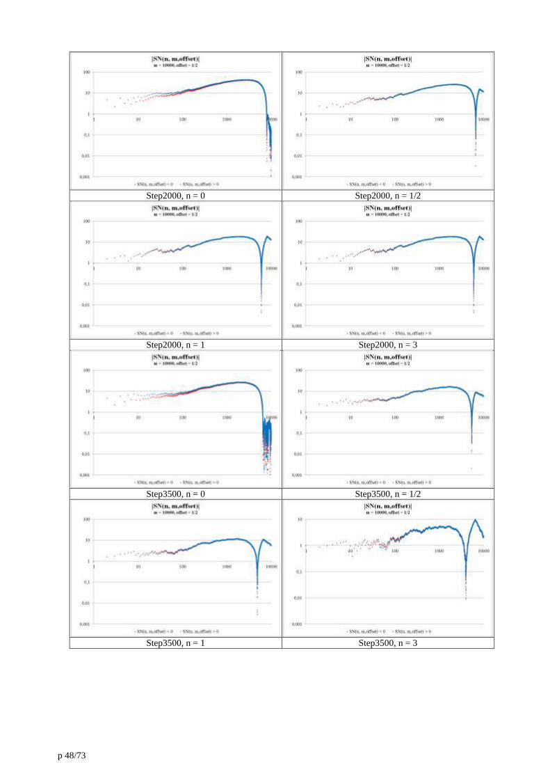
p 48/73

Step2000, n = 0 Step2000, n = 1/2

Step2000, n = 1 Step2000, n = 3

Step3500, n = 0 Step3500, n = 1/2

Step3500, n = 1 Step3500, n = 3

p 49/73

Step10000, n = 0 Step10000, n = 1/2

Step10000, n = 1 Step10000, n = 3

The reader can clearly see that the graphs tend after random shuffles towards a dispersal of ratio between 0,1 and 10

with very many getaways to much lower values, meaning a majorated asymptotic ratio (as desired).

Being random results, each test (steps 0 to 10000) results in another point cloud. The graphs below are various examples

for n = 1/2 (to be compared to the previous ones).

p 50/73

Taking the last graph (thus n = 1/2, m = 10000, offset = 1/2) and writing down

SN(n, m, offset) = NSN(n, m, offset)/DSN(n, m, offset)

where NSN(n, m, offset) is the numerator and DSN(n, m, offset) the denominator of SN(n, m, offset) according to the

definition adopted above (i.e. with division by m), we get the representative graphs of m.NSN(n, m, offset) and

m.DSN(n, m, offset) on one hand and of NSN(n, m, offset) and DSN(n, m, offset) on the other hand underneath.

The denominator forms lower and upper bounds of the rarely crossed numerator.

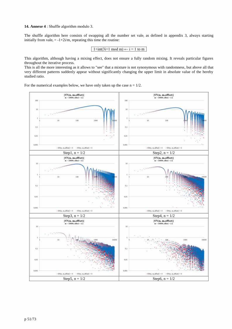
p 51/73

14. Annexe 4 : Shuffle algorithm modulo 3.

The shuffle algorithm here consists of swapping all the number set valei as defined in appendix 3, always starting

initially from valei = -1+2i/m, repeating this time the routine:

1+int(3i+1 mod m) ← i = 1 to m

This algorithm, although having a mixing effect, does not ensure a fully random mixing. It reveals particular figures

throughout the iterative process.

This is all the more interesting as it allows to "see" that a mixture is not synonymous with randomness, but above all that

very different patterns suddenly appear without significantly changing the upper limit in absolute value of the hereby

studied ratio.

For the numerical examples below, we have only taken up the case n = 1/2.

Step1, n = 1/2 Step2, n = 1/2

Step3, n = 1/2 Step4, n = 1/2

Step5, n = 1/2 Step6, n = 1/2

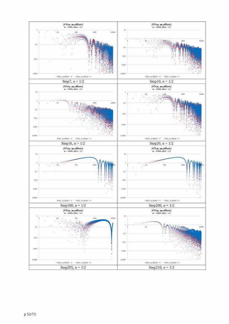
p 52/73

Step7, n = 1/2 Step10, n = 1/2

Step16, n = 1/2 Step20, n = 1/2

Step100, n = 1/2 Step200, n = 1/2

Step205, n = 1/2 Step210, n = 1/2

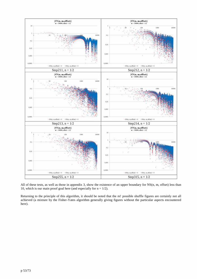
p 53/73

Step211, n = 1/2 Step212, n = 1/2

Step213, n = 1/2 Step214, n = 1/2

Step255, n = 1/2 Step315, n = 1/2

All of these tests, as well as those in appendix 3, show the existence of an upper boundary for NS(n, m, offset) less than

10, which is our main proof goal here (and especially for n = 1/2).

Returning to the principle of this algorithm, it should be noted that the m! possible shuffle figures are certainly not all

achieved (a mixture by the Fisher-Yates algorithm generally giving figures without the particular aspects encountered

here).

p 54/73

15. Annexe 5 : Comparison of random sums to alternating sums of integers.

The graphs below represent the m-based evolution (in abscissa of the graphs) of:

m

lim (1/m) ∑ vi.in (84)

m → +∞ i = 0

for :

- TR1 : on one hand vi = 2.ai-1 taking uniform random values in interval [-1,1],

- TR2 : on the other hand vi =(-1)i-1

.

The first case is represented by the green graphs (TR1) and their evolution is necessarily "chaotic".

The second case is represented by the blue graphs (TR2). The sum passes at each step m to a sign value opposite to the

previous one, hence the two paths on either side of the axis y = 0.

The TR2 plots are unique for n given in advance. This is not the case for TR1 plots, which can have significantly

different shapes. Each time, we gave for TR1 and for given n two examples : the first one with getaway from the TR2

frame, the second remaining "wisely" inside. For both, we can easily find either worse or better examples.

Comparisons are made with an offset 1/2 between the chosen n-powers for the two plots.

TR1 n = 0

TR2 n = 0,5

TR1 n = 0

TR2 n = 0,5

TR1 n = 0,25

TR2 n = 0,75

TR1 n = 0,25

TR2 n = 0,75

p 55/73

TR1 n = 0,5

TR2 n = 1

TR1 n = 0,5

TR2 n = 1

TR1 n = 0,75

TR2 n = 1,25

TR1 n = 0,75

TR2 n = 1,25

p 56/73

16. Annexe 6 : Extremums of SN(n,m,offset) sums.

The table below is the list of extremum reading of the sums SN(n,m,offset), offset = 1/2, imax = m. It corresponds to

graphs 13, 14 and 15 page 19. The n = 1/2 line that we are particularly interested in is highlighted in red.

n imax = 100 imax = 1000 imax = 10000 imax = 101 imax = 1001 imax = 10001

-100 0,999997 0,999997 0,999997 0,999997 0,999997 0,999997

-10 1,0017 1,0017 1,0017 1,0017 1,0017 1,0017

-5 1,0698 1,0698 1,0698 1,0698 1,0698 1,0698

-2 1,8162 1,8153 1,8153 1,8138 1,8153 1,8153

-1,5 2,4365 2,4213 2,4191 2,4030 2,4178 2,4188

-1 4,3460 4,2325 4,2065 3,6999 4,0174 4,1374

-0,9 5,8133 5,4294 5,2526 4,4354 4,8736 5,0316

-0,8 6,6439 5,8860 5,9122 4,2096 4,7106 5,2863

-0,7 9,6003 8,9957 8,9187 4,4996 5,6193 6,6502

-0,6 21,4529 15,5279 14,6416 5,3532 5,4459 6,5652

-0,55 38,5347 30,9405 27,8464 4,9289 5,6343 6,5979

-0,51 226,6491 181,4476 142,3444 5,7834 6,6625 6,8648

-0,5 → ∞ → ∞ → ∞ 5,0530 5,5991 6,8586

-0,49 198,4679 166,3879 159,3619 5,0036 6,1388 7,6857

-0,45 44,3201 36,5606 29,2279 5,5577 6,6312 6,9199

-0,4 20,7778 17,7747 14,1354 5,2037 6,2870 6,3649

-0,3 10,3032 8,8543 8,2375 4,7932 5,5222 6,1580

-0,2 7,8684 6,1053 6,1934 5,0836 4,9676 5,5606

-0,1 5,6482 5,1753 4,9325 4,4771 4,6629 4,7299

0 5,9506 5,5753 5,2768 5,1643 5,2891 5,1799

0,1 4,3633 4,7950 4,0256 4,0601 4,6708 3,9863

0,2 4,3467 3,7941 4,2058 4,1830 3,7534 4,1963

0,3 3,8411 3,9290 4,3080 3,7486 3,8979 4,3097

0,4 3,3384 3,3270 3,3044 3,3121 3,3229 3,3011

0,5 3,2685 3,3726 3,2147 3,1337 3,2884 2,9966

0,6 3,1046 2,8481 2,8662 2,9030 2,8282 2,7644

0,7 2,5353 3,3440 2,7954 2,5502 2,9401 3,1442

0,8 2,7294 2,5062 2,5401 2,8621 3,2066 3,0275

0,9 2,5822 2,8370 2,5541 2,4386 2,5995 2,5583

1 2,6340 2,4761 2,8728 2,3287 2,3434 2,4275

1,1 3,1114 2,5096 2,4488 2,2227 2,4573 2,6889

1,2 2,2842 2,2278 2,5598 2,3496 2,5383 2,2444

1,3 2,0528 2,7465 2,4720 2,1116 2,4144 2,2972

1,4 2,0675 2,1444 2,1465 2,1071 2,1853 2,1631

1,5 2,3914 2,1372 1,9381 2,2408 2,3153 2,5934

2,5 2,1669 1,8311 1,7609 1,9002 1,7010 2,0826

5 1,3727 1,2500 1,2456 1,2797 1,3416 1,4386

10 0,8551 1,0008 0,9946 0,9135 0,9812 1,0025

25 0,5298 0,6463 0,6131 0,5250 0,6345 0,6140

50 0,3241 0,4273 0,4047 0,3284 0,4235 0,4216

75 0,2496 0,3724 0,3229 0,2417 0,3069 0,3717

p 57/73

17. Annexe 7 : Effect of Fisher-Yates algorithm on weighed prime numbers sums.

Distribution 𝔇0 The NSP(n, m, 1/2) and NSN(n, m, 1/2) curves relative to prime numbers and integers trivially overlap when n = 0 for an identical ordered distribution on both sums. Below we present the gradual evolution of NSP(n, m, 1/2) compared to NSN(n, m, 1/2) by increasing n without changing the distribution. This shows that, in this case, if |NSN(n, m, 1/2)| is bounded then |NSP(n, m, 1/2)| is too. Two sets of tests (and thus two graphs per box), among the 10000! possible, are presented in such a way as to give the reader an idea of the differences of evolution from one to the other. The initial curve is obviously the same for both sets of tests. The first drawings are those of step 0 before application of the Fisher-Yates algorithm.

𝔇0 sorted, n = 0 𝔇0 sorted, n = 1/4

p 58/73

𝔇0 sorted, n = 1/2 𝔇0 sorted, n = 3/4

We then reassign the weights (keeping the same on the same i's) from the random distribution. We proceed for n = 1/2

which is the interesting case.

The effect of redistribution by the Fisher-Yates algorithm is a slight pulling together of the curves |NSN(n,m,1/2)| et |NSP(n,m,1/2)|. This further illustrates that if |NSN(n,m,1/2)| is bounded, then |NSP(n,m,1/2)| is too.

𝔇0 mélange 5/10, n = 1/2 𝔇0 mélange 6/10, n = 1/2

p 59/73

𝔇0 mélange 7/10, n = 1/2 𝔇0 mélange 8/10, n = 1/2

𝔇0 mélange 9/10, n = 1/2 𝔇0 mélange 10/10, n = 1/2

p 60/73

Distribution 𝔇1 We observed for the 𝔇0 distribution that the NSP(n,m,1/2) and NSN(n,m,1/2) curves are close. We therefore prefer to give below NSP(n,m,1/2) and the ratio NSP(n,m,1/2)/NSN(n,m,1/2). If the latter is finite and NSN(n,m,1/2) is bounded, then |NSP(n,m,1/2)| is necessarily bounded. We have represented in red the |NSP(n,m,1/2)| points such as the ratio NSP(n,m,1/2)/NSN(n,m,1/2) is greater than 10. This makes it easy to see that a large ratio occurs when NSN(n,m,1/2) approaches 0. Thus all these points are 'safe' regarding the bounded value of NSP(n,m,1/2) We limit ourselves to an example of evolution among the 10,000! possible.

𝔇1, n = 0 𝔇1, n = 1/4

𝔇1, n = 1/2 𝔇1, n = 3/4

The charts below give two other examples among the 10,000! possible cases here for n = 1/2.

𝔇1, n = 1/2 𝔇1, n = 1/2

p 61/73

Distribution 𝔇2 Previous remarks apply to the 𝔇2 distribution.

𝔇2, n = 0 𝔇2, n = 1/4

𝔇2, n = 1/2 𝔇2, n = 3/4

The graphs below give two other examples of among the 10,000! possible cases here for n = 1/2. The dispersion is

different, but the upper bound values, which interest us here, change little.

𝔇2, n = 1/2 𝔇2, n = 1/2

p 62/73

18. Annexe 8 : Accélération de l’effet de convergence.

Let us have R(E,c=1) the following ratio of Euler products :

∏ (1-api/pi)

R(E,c) = pi ∈ 𝒫

∏ (1-M/pi)

pi ∈ 𝒫

Here M is the average of api. The R(E,c) ratio tends towards its limit relatively slowly as shown in grapghics 37 and 38.

We propose to visualize the asympotic behavior of this report in an artificial way, but in accordance with reality. We do

this while moving completely away from the real values of the expressions. The only goal here is to show that the

progression to infinity follows a perfect horizontal.

We place ourselves in the case of a 𝔇1∞ distribution, i.e. api is of the form api = sin(2π.alea()).si(pi = 3 mod 4, 0, 1).√pi.

We first simplify this writing by replacing ci = si(pi = 3 mod 4, 0, 1) by ci = ent(2.alea()), i.e. ci takes the value 0 for 50%

of the pi and 1 for the other 50% completely randomly. This allows us to get rid of a link to pi that is ineffective anyway

and useless here. Besides the result that we seek to establish would be the same by systematically taking ci = 1. What

matters is that the absolute value |api/pi| < 1/√pi → 0 and therefore 1-api/pi → 1.

We then keep the term pi unchanged until the i = 100 index, but we artificially replace its value for further indices using :

pi+1 = pi+(int(ln(pi)))r

This allows to get in an accelerated way large pi numbers. These are no longer prime numbers but it is absolutely

irrelevant.

Each calculation gives another graph and here we give two samples for each r value.

Case r = 1.

This one is "identical" to the case where pi actually represents all the prime numbers.

Cas r = 2.

The maximum abscissa pi is multiplied by a factor of 20 compared to case r = 1.

p 63/73

Cas r = 3.

The maximum abscissa pi is multiplied by a factor of 500 compared to case r = 1.

Cas r = 4.

The maximum abscissa pi is multiplied by a factor of 20 000 compared to case r = 1.

Cas r = 5.

The maximum abscissa pi is multiplied by a factor of 1 000 000 compared to case r = 1.

p 64/73

19. Annexe 9 : Comparison of distribution 𝔇2 to its approximation.

The aim here is to compare the values obtained by drawing the actual distribution curve of the 𝔇2 distribution, namely

cos(π.(f

-1(x)-1)), where 0 ≤ x ≤ 1 and f(u) = u-sin(2π.u)/2π, with the approximate alternative distribution curve defined

by if(x < 1/2, -1, 1).cos(arcsin(c.((1-x).x)ln(c)/ln(4)

), where c is chosen in such a way that the variance of this approximation

is the same as that of the actual curve (i.e. 1/4).

Research of c. Programming

The calculation of c is obtained by the computer program underneath where the solution c must give y = 0.

\ p 250 \\ accuracy of adjustable calculation (precision shown here far superior to our need)

c1 = 3/2; c2 = 3.1/2; V = 1/4; \\ V adjustable

for(i = 1,10000, \\ adjustable

b1 = log(c1)/log(4);

y1 = intnum(x = 0, 1, c1*c1*((x-x*x)^(2*b1)))-(1-V); \\ double-exponential method to evaluate integrals

b2 = log(c2)/log(4);

y2 = intnum(x = 0, 1, c2*c2*((x-x*x)^(2*b2)))-(1-V);

if(abs(y2) > 1E-200, c = c1-y1*(c2-c1)/(y2-y1); c1 = c2; c2 = c, print("i = "i); break));

print("V = "V); print("c = "c2); print("y ="y2)

i = 11

V = 1/4

c = 1.54210744624138725479407564146789189851624581044607868460263491833070140504

39574124259838383646073973979191281412482929566736576897856674528727628144835460

25726294480890464757185320256871047925179056938069643713861742857691067772684359

035758954379903

y =0.E-250

Comparison of distribution 𝔇2 to its approximation

At the global scale of the graph, the differences between the two curves are not visible.

A few closer views, however, show that they are not identical. Between x = 0 and x = 1/2, the approximate curve first

merges with the actual curve, then passes slightly above (maximum gap 4/1000 versus ordinate near abscissa 0,007),

returns to merge, then passes slightly below (maximum gap 1/1000 versus ordinate on a wide band of abscissas) and

merges again to very little with it. From x = 1/2 to x = 1, there is the exact symmetrical.

p 65/73

p 66/73

20. Annexe 10 : Evolution of the average of the error term (or quadratic opposite) ap.

The curves correspond to the appendix 1 list. The abscissa is graduated by the prime numbers p i. Their index ranges

from 1 to 100000 (p1 = 2, p100000 = 1299709).

The graphs show a trend towards the theoretical value of algebraic ranks, but this trend is far from being stabilized at

this stage of calculation.

p 67/73

p 68/73

21. Annexe 11 : Deviation to the distributions.

The curves are those in the appendix 1 list. The abscissa is graduated by the i index of prime numbers pi. Their index

ranges from 1 to 100000 (p1 = 2, p100000 = 1299709).

The deviations to the theoretical curve are visible because i is finite.

Graphs 49, 50 et 51

p 69/73

Graphs 52, 53 et 54

p 70/73

Graphs 55, 56 et 57

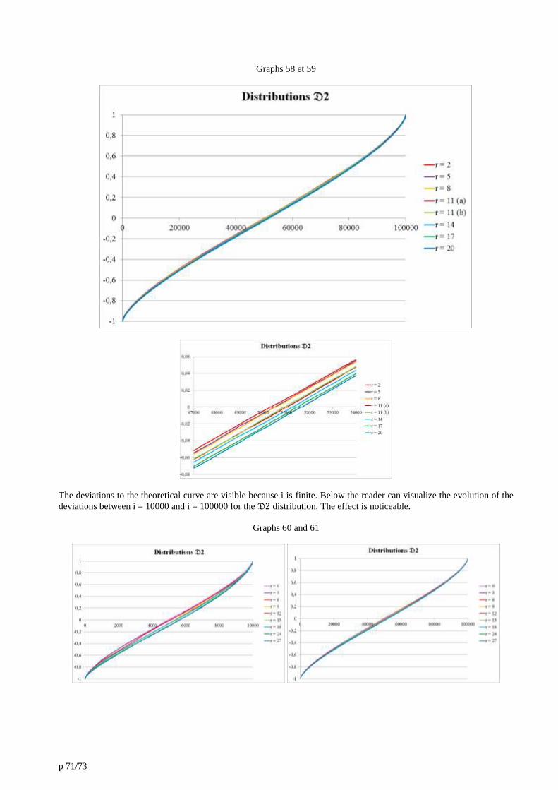
p 71/73

Graphs 58 et 59

The deviations to the theoretical curve are visible because i is finite. Below the reader can visualize the evolution of the

deviations between i = 10000 and i = 100000 for the 𝔇2 distribution. The effect is noticeable.

Graphs 60 and 61

p 72/73

22. Annexe 12 : Evolution of Euler products ratios.

The elliptical curves below correspond to those on the appendix 1 list. The abscissa is graduated by the i index of prime

numbers pi. Their index ranges from 1 to 100000 (p1 = 2, p100000 = 1299709).

Let us have M(E,n) the arithmetic average of the error terms api (the opposite of which tends towards the arithmetic

rank). The graphs show, for i increasing up to n = 100000, the variation of the ratio :

∏ 1-M(E,100000)/pi

pi ≤ p100000

∏ 1-api/pi

pi ≤ p100000

The expected effect is a gradual convergence towards a constant value. The positioning of one curve relatively to

another is totally arbitrary (and is not in the curve's rank order).

p 73/73