Journal of Monetary Economics 47 (2001) 449–475

Common cycles and the importance oftransitory shocks to macroeconomic

aggregates$

Jo*ao Victor Isslera,*, Farshid Vahidb

aGraduate School of Economics, EPGE, Getulio Vargas Foundation, P. de Botafogo 190 s. 1100,

Rio de Janeiro, RJ 22253-900, BrazilbDepartment of Econometrics and Business Statistics, Monash University, Clayton, Victoria 3168,

Australia

Received 15 October 1996; received in revised form 27 January 2000; accepted 23 June 2000

Abstract

Although there has been substantial research using long-run co-movement(cointegration) restrictions in the empirical macroeconomics literature, little or nowork has been done investigating the existence of short-run co-movement (commoncycles) restrictions and discussing their implications. In this paper we first investigate the

existence of common cycles in a aggregate data set comprising per-capita output,consumption, and investment. Later we discuss their usefulness in measuring the relativeimportance of transitory shocks. We show that, taking into account common-cycle

restrictions, transitory shocks are more important than previously thought at business-cycle horizons. The central argument relies on efficiency gains from imposing theseshort-run restrictions on the estimation of the dynamic model. Finally, we discuss how

the evidence here and elsewhere can be interpreted to support the view that nominal

$We gratefully acknowledge comments from Heather Anderson, Wouter den Haan, Robert F.

Engle, Pedro C. Ferreira, Clive W.J. Granger, Takeo Hoshi, Afonso A. Mello Franco, Charles

Plosser, Valerie A. Ramey, and an anonymous referee, who are not responsible for any remaining

errors in this paper. Jo*ao Victor Issler gratefully acknowledges support form CNPq-Brazil and

PRONEX, while Farshid Vahid gratefully acknowledges support form The Bush Program in the

Economics of Public Policy.

*Corresponding author. Tel.: +55-21-559-5833; fax: +55-21-553-8821.

E-mail addresses: jissler@fgv.br (J.V. Issler).

0304-3932/01/$ - see front matter r 2001 Elsevier Science B.V. All rights reserved.

PII: S 0 3 0 4 - 3 9 3 2 ( 0 1 ) 0 0 0 5 2 - 6

shocks may be important in the short run. r 2001 Elsevier Science B.V. All rights

reserved.

JEL classification: E32; C32; C53

Keywords: Trend-cycle decomposition; Common cycles; Forecasting; Cointegration

1. Introduction

It is a well-known stylized fact in macroeconomics that economic datadisplay co-movement. For example, Lucas (1977, Section 2) reports thatoutput movements across broadly defined sectors have high coherence. On theother hand, Kosobud and Klein (1961) document that aggregate consumption,investment and output follow balanced growth paths. While the firstobservation is a statement about short-run co-movement, which imposesrestrictions on transitional dynamics of sectoral outputs, the second is astatement about long-run co-movement, imposing the restriction thatmacroeconomic aggregates cannot drift apart over time. These two types ofrestrictions play an important role in determining the dynamic behavior ofmacroeconomic time series.Up to the present, using the econometric concept of cointegration (Engle and

Granger, 1987), there has been a fair amount of research on long-run co-movement and its implications, which has shown convincingly that macro-economic aggregates are cointegrated. Long-run restrictions have been largelyused in econometrics for several purposes, including estimation (Engle andGranger) and forecasting (Engle and Yoo, 1987). In the applied macro-economics literature they have been used for the structural identification ofeconomic shocks (Blanchard and Quah, 1989; King et al., 1991 inter-alia). InBlanchard and Quah, permanent shocks to output with no effect onunemployment are labelled ‘‘supply’’ shocks, whereas in King et al. thepermanent shock with identical impacts on output, consumption, andinvestment is labelled ‘‘productivity’’ shock. Both then proceed to measurethe relative importance of permanent shocks in variance–decomposition andimpulse–response exercises. A similar strategy has recently been followed byGalı́ (1999), who uses long-run restrictions to identify ‘‘productivity’’ shocksand examine how the predictions of a class of Real-Business-Cycle models fitthe data.Although the use of low-frequency (cointegration) restrictions to decompose

economic series into trends and cycles is widely used, this is by no means theonly type of restrictions that can be employed to that end. High-frequencyrestrictions (common cycles) can also be used in conjunction with cointegrationrestrictions, whenever the latter exist. This was initially shown by Vahid and

J.V. Issler, F. Vahid / Journal of Monetary Economics 47 (2001) 449–475450

Engle (1993), who proposed the use of the common trends and common cyclesmethod, later applied to a sectoral output data set by Engle and Issler (1995);see also Engle and Kozicki (1993) for a broader view of these ‘‘commonfeatures’’.For a given data set, the joint use of common-trend and common-cycle

restrictions to identify permanent and transitory shocks has a clear advantageover the use of common-trend restrictions alone. First, there is the econometricissue of relative efficiency. Obviously, if common-cycle restrictions are correctlyimposed, estimates of the dynamic model (usually a vector autoregression) aremore precise, leading to a more precise measurement of the relative importanceof permanent and transitory shocks. Indeed, if two series have a common cycletheir impulse–response functions are exactly colinear (Vahid and Engle, 1997).Thus, variance–decomposition and impulse–response calculations will be basedon a reduced set of parameters. Second, there is the issue of the horizon whenmeasuring the relative importance of shocks. For both methods, the relativeimportance of permanent and transitory shocks should not differ much forlong horizons, since both impose the same long-run restrictions. However, theyhave the potential to be different for short horizons, because restrictions onshort-run dynamics are imposed by only one of them.This potential distinction is important for two reasons. On the one hand, the

real usefulness of time series models is in their predictions at business-cyclehorizons, since predictions further into the future are less precise and are alsodiscounted more heavily by economic agents. On the other hand, while mostresearchers agree that nominal shocks have a limited (or no) effect on the long-run behavior of macroeconomic aggregates, there is no agreement on theireffect at business-cycle horizons. This is why the relative efficiency resultmatters; a method using common-trend and common-cycle restrictions willdeliver a more precise measurement of the relative importance of permanentand transitory shocks for the horizon that agents care most about and forwhich debate in the literature continues.The goal of this paper is to examine whether US per-capita output,

consumption, and investment share common cycles using the common trendsand common cycles method discussed in Vahid and Engle (1993). There, long-run co-movement is characterized as common stochastic trends and short-runco-movement is characterized as common cyclical components that aresynchronized in phase but may have different amplitudes. Using efficientestimates of a vector autoregressive model, which is restricted to producecommon trends and common cycles, we calculate the relative importance ofpermanent and transitory shocks. We later confirm the efficiency gains for ourdata set in an out-of-sample forecasting exercise.Investigating the existence of common cycles is interesting in its own right,

given that this is a theoretical implication of several dynamic macroeconomicmodels. Examples of these models are provided below. Using a more efficient

J.V. Issler, F. Vahid / Journal of Monetary Economics 47 (2001) 449–475 451

trend-cycle decomposition of the data we are able to answer more precisely akey question in macroeconomics, considered, among others, by Nelson andPlosser (1982); Watson (1986); Campbell and Mankiw (1987); Cochrane (1988,1994); King et al. (1991); and Galı́ (1999): what is the relative importance ofpermanent and transitory shocks in explaining the variation of macroeconomicdata?Our empirical findings confirm the presence of common cycles in the data.

The variance–decomposition results show that, for output and investment,transitory shocks are important in explaining their variation. On the otherhand, permanent shocks are the most important source of variation forconsumption, whose behavior is close to a martingale (Hall, 1978 and Flavin,1981). Contrasting our variance decomposition results with those of King et al.(1991), who only considered cointegration restrictions to identify permanentand transitory shocks, illustrates that ignoring common-cycle restrictions leadsto non-trivial differences in the relative importance of transitory shocks.Indeed, we find transitory shocks to be more important than previous researchhas found. This is true especially at business-cycle horizons, illustrating theadvantage of the method used here. These findings are consistent with therecent results in Galı́ (1999)Fshowing that nominal (transitory) shocks arecritical in explaining several features of aggregate data for G-7 countries, andin den Haan (1996)Fshowing that demand shocks may be relevant forexplaining the conditional correlations of output and prices and of hours andreal wages in the short run.Section 2 discusses several dynamic macroeconomic models that deliver

common trends and common cycles for macroeconomic aggregates. Section 3discusses testing for common trends and cycles as well as the estimation ofdynamic systems under long- and short-run co-movement restrictions. Adetailed explanation of the methodology used is presented in the AppendicesA–C. Section 4 presents empirical results and Section 5 concludes.

2. Theory and testable implications

Common trends and common cycles appear in the macroeconomicsliterature in several theoretical models. Here we discuss a few examples. Inthe dynamic stochastic general equilibrium model of King et al. (1988), output,consumption and investment have a common trend1 and a common cycle as aresult of the optimizing behavior of the representative agent. Cointegrationcomes from having a common forcing variable (productivity) and a commoncycle arises from the fact that the transitional dynamics of the system is a

1The same result is true using the endogenous growth model of Romer (1986). This makes these

two models observationally equivalent in cointegrating tests.

J.V. Issler, F. Vahid / Journal of Monetary Economics 47 (2001) 449–475452

(linear) function of a unique factorFthe deviation of the capital stock from itssteady-state value. Although these results are obtained under log-utility, full-depreciation of the capital stock, and Cobb–Douglas technology, they can begeneralized for a variety of parameterizations under a quadratic approximationof the value function. The closed-form solutions for the logarithms of output,consumption and investment are, respectively,

logðYtÞ ¼ logðXpt Þ þ %yþ pyk #kt;

logðCtÞ ¼ logðXpt Þ þ %cþ pck #kt;

logðItÞ ¼ logðXpt Þ þ %i þ pik #kt; ð2:1Þ

where logðXpt Þ ¼ mþ logðXp

t@1Þ þ ept is the random-walk productivity processin production, %y, %c and %i are the steady-state values of logðYt=X

pt Þ; logðCt=X

pt Þ,

and logðIt=Xpt Þ, respectively, and pjk; j ¼ y; c; i is the elasticity of variable j with

respect to deviations of the capital stock from its stationary value ðk̂tÞ.2 From

(2.1) it is straightforward to verify that these variables have a common trendðlogðXp

t ÞÞ, and a common cycle ðk̂tÞ. The following linear combinations have notrend:

logðYtÞ@logðCtÞ;

logðYtÞ@logðItÞ ð2:2Þ

and logðYtÞ, logðCtÞ, and logðItÞ are cointegrated in the sense of Engle andGranger (1987), with (2.2) showing two (linearly) independent cointegratingrelationships. The following linear combinations have no cycle:

pck log ðYtÞ@pyk log ðCtÞ;

pik log ðYtÞ@pyk log ðItÞ ð2:3Þ

and logðYtÞ, logðCtÞ, and logðItÞ have a common cycle in the sense of Vahid andEngle (1993), with (2.3) showing two (linearly) independent cofeaturecombinations.To elaborate more on this issue, consider the first differences of the

logarithm (i.e. growth rate) of system (2.1):

D logðYtÞ ¼ ept þ pykD #kt;

D logðCtÞ ¼ ept þ pckD #kt;

D logðItÞ ¼ ept þ pikD #kt: ð2:4Þ

2As noted by King et al. (1988), the above theoretical model is too simplistic to be taken as a full

characterization of the data-generating process, since its only source of randomness is the

productivity shock, making the system in (2.1) stochastically singular. There is an imbedded

identity in this system:

ðpik@pckÞ ðlog ðYtÞ@ %yÞ ¼ ðpik@pykÞ ðlog ðCtÞ@ %cÞ þ ðpyk@pckÞ ðlog ðItÞ@%iÞ:

J.V. Issler, F. Vahid / Journal of Monetary Economics 47 (2001) 449–475 453

Given that ept is white noise, Eqs. (2.4) show that all the (short-run) serialcorrelation of macroeconomic aggregates is due to a single common factorðD #ktÞ. Thus, ‘‘cycles’’ in D logðYtÞ, D logðCtÞ, and D logðItÞ are synchronized,but amplitudes may differ since the pjk’s may be different.In the class of partial equilibrium models, Campbell (1987) shows that

saving ðStÞ can be written as a function of expected future-income variationsEtðDYtþsÞ:

St ¼ @XNs¼1

rsEtðDYtþsÞ; ð2:5Þ

where Et is the conditional expectation operator using information up toperiod t, and r is the one-period discount factor for future income ðYtþsÞ. Sincesaving is the difference between disposable income and consumption, which by(2.5) is stationary, consumption and disposable income must cointegrate if Yt isan integrated series.For partial equilibrium models in the tradition of Hall (1978) and Flavin

(1981), consumption is a martingale. Hence, its first difference has no serialcorrelation even if the (differenced) income process is serially correlated. Thus,consumption and income fail to have common cycles. However, if a proportionof the population follows the ‘‘rule of thumb’’ of consuming their incomeentirely in every period, Campbell and Mankiw (1989) show that aggregateconsumption and aggregate income will have a common cycle as a result of thismyopic behavior.Letting ðC1t;Y1tÞ and ðC2t;Y2tÞ be the consumption-income pairs of

‘‘permanent income’’ and ‘‘myopic’’ agents, respectively, and letting ðCt;YtÞdenote the aggregate consumption-income pair, with l ¼ Y2t=Yt measuring theincome proportion of myopic agents, Campbell and Mankiw show that:

DCt ¼ lDYt þ ð1@lÞmt; ð2:6Þ

where mt is proportional to the innovation in Y1t. Since mt is unpredictable, andsince DYt is usually serially correlated, Eq. (2.6) shows that all the serialcorrelation of DCt comes from DYt. In this case, the cycles of Yt and Ct aresynchronized. Notice that the amplitude of the cycle in consumption is anincreasing function of the importance of myopic agents ðlÞ.The examples discussed above suffice to show that common trends and

common cycles for macroeconomic aggregates can be the result of eitheroptimal or myopic behavior, and are a feature of partial and generalequilibrium models. This in itself motivates their investigation. There is anadditional reason to study them: common trends and common cycles represent,respectively, low- and high-frequency restrictions on multivariate data sets.Whenever these restrictions are present, imposing them can considerablyreduce the number of estimated parameters in time series models, leading toefficiency gains in estimation.

J.V. Issler, F. Vahid / Journal of Monetary Economics 47 (2001) 449–475454

3. Estimation and testing

This section discusses testing for common trends and cycles, andimplications of their existence for the efficient estimation of dynamic modelsof macroeconomic aggregates. We present in Appendices A–C the formaldefinitions of common trends and cycles, different representations formacroeconomic aggregates under their presence, and the trend-cycle decom-position method used here.Following King et al. (1991), it is useful to note that the reduced form for a

(linear) system containing (the log of) output, consumption and investment isnested in the general dynamic framework of vector autoregressions (VAR’s). Ifthere are common trends in the data, the VAR has cross-equation restrictionsas shown by Engle and Granger (1987). Thus, we can reduce the number ofparameters of the dynamic representation by estimating a vector error-correction model (VECM) which takes these restrictions into account.Common cycles impose extra restrictions on this dynamic system (Vahid andEngle, 1993). In this case it is possible to further reduce the number ofparameters in the VECM. Efficient estimation requires estimating a restrictedVECM, which takes into account the common cyclical dynamics present in thefirst differences of the data; see Eqs. (2.4) and (2.6) for example.Tests for cointegration are not discussed in any length here, since this

literature is now well known. We employ Johansen’s (1988, 1991) technique,which estimates the number of linearly independent cointegrating vectors ðrÞ.Testing for common cycles amounts to searching for independent linearcombinations of the (level of the) variables that are random walks, thus cyclefree. The test therefore is a search for linear combinations of the firstdifferences of the variables whose correlation with the elements of the pastinformation set in the right-hand side of the VECM will be zero. This can bedone by testing for zero canonical correlations between the first differences ofthe variables and the elements of the past information set. This test is in effecttesting for cross-equation restrictions on the parameters of the VECM; seeVahid and Engle (1993).Assuming that output, consumption and investment have one stochastic

trend, 3 and that the two cointegrating relationships are, respectively ðlog ðCt

=YtÞÞ and ðlog ðIt=YtÞÞ, the test for common cycles and the fully efficientestimation of the restricted VECM entails the following steps:

1. Determine p, the required number of lags in the VECM that adequatelycaptures the dynamics of the system.

3This is not to say that the common-cycle test is not applicable when variables have deterministic

rather than stochastic trends. In fact, common cycles are about co-movement in detrended series,

regardless of the form of the trend. We explain the procedure for the case of stochastic trends

because it is more relevant to the present paper. The case of deterministic trend is straightforward.

J.V. Issler, F. Vahid / Journal of Monetary Economics 47 (2001) 449–475 455

2. Compute4 the sample squared canonical correlations between fD logðYtÞ;D logðCtÞ;D logðItÞg and flogðCt@1=Yt@1Þ; logðIt@1=Yt@1Þ;D logðYt@1Þ;D logðCt@1Þ;D logðIt@1Þ;y; D logðYt@pÞ;D logðCt@pÞ;D logðIt@pÞg, labelledli, i ¼ 1;y; n, where n is the number of variables in the system (n equalsthree in this case).

3. Test whether the first smallest s canonical correlations are zero bycomputing the statistic:

@TXsi¼1

logð1@liÞ;

which has a limiting w2 distribution with sðnpþ rÞ@sðn@sÞ degrees offreedom under the null, where r is the number of cointegrating relationships(r equals two in our example). In the absence of identities in the system, themaximum number of zero canonical correlations that can possibly exist isn@r (n@r is one in our example, since we assumed two cointegratingvectors).

4. Suppose that s zero canonical correlations were found in the previous step.Use these s contemporaneous relationships between the first differences as spseudo-structural equations in a system of simultaneous equations.Augment them with n@s equations from the VECM and estimate thesystem using full information maximum likelihood (FIML). The restrictedVECM will be the reduced form of this pseudo-structural system.

In addition to leading to a parsimonious model, the existence of unpredictablelinear combinations of the first differences may allow us to readily identify theshocks with permanent effects. Take, for example, the model of King et al.(1988) discussed above. There,

pckD log ðYtÞ@pykD log ðCtÞ ¼ ðpck@pykÞept ;

pikD log ðYtÞ@pykD log ðItÞ ¼ ðpik@pykÞept : ð3:1Þ

Either of these two equations identify ept , given knowledge of pyk, pck, and pik.Along the same lines, for the model of Campbell and Mankiw (1989), we have:

DCt@lDYt ¼ ð1@lÞmt; ð3:2Þ

which, given l, identifies mt, the shock to permanent income of the type oneconsumer.This form of shock identification is much simpler than the method employed

by King et al. (1991), since it only requires knowledge of cointegrating andcofeature vectors; see Appendices A–C. The latter requires inverting theautoregressive representation. Also, since we impose testable long- and short-run restrictions to the VAR, we achieve more efficient estimates of VAR

4This can be easily done using PROC CANCORR in SAS. Alternatively, a GAUSS code for

calculating canonical correlations and the test statistic for common cycles is available upon request.

J.V. Issler, F. Vahid / Journal of Monetary Economics 47 (2001) 449–475456

coefficients. This leads to more efficient estimates of impulse responses andvariance decompositions, since these are based on a more parsimonious model.It is important to understand the possible differences in results from using

the two methods. If the long-run restrictions imposed by both methods are thesame, impulse–response and variance–decomposition results will be similar forlong horizons (being exactly the same in the infinite horizon). However, theyhave the potential to differ at business-cycle horizons, since only the methodused here imposes short-run co-movement restrictions. Given the efficiencygains discussed above, our variance–decomposition and impulse–responseresults will be more precise at short horizons. As argued above, this isimportant for economic agents, who discount future events more heavily, andthus care more about what happens at business-cycle horizons. It is alsoimportant as a tool in evaluating theoretical models in short horizons,especially regarding the potential importance of nominal shocks.Since the efficiency-gains result is theoretical, we compare out-of-sample

forecasts between the restricted and the unrestricted VECM to substantiatethat these gains are relevant for the present data set. We find that the formerperforms better.

4. Empirical evidence

The data being analyzed consist of ðlogÞ real U.S. per-capita privateoutputFy, personal consumption per-capitaFc, and fixed investment per-capitaFi. The data were extracted from Citibase on a quarterly frequency.5

Although Citibase has data available from 1947:1 to 1994:2, we used only1947:1–1988:4 in estimation, in order to match the sample period used in Kinget al. (1991), thus making results directly comparable.The plot of (logged) per-capita real output, consumption and investment is

presented in Fig. 1. There are two striking characteristics. First, the data areextremely smooth (typical of Ið1Þ data) and appear to be trending together inthe long run. Second, the data show similar short-run behavior: duringrecessions all three aggregates drop. However, investment drops much morethan consumption and output, and the latter drops more than consump-tionFthe most insensitive series to recessions.Tests for cointegration were performed using Johansen’s (1988, 1991)

technique and are presented in Table 1. Critical values were extracted fromOsterwald-Lenum (1992). We conclude that the cointegrating rank r is two.This implies the existence of a common stochastic trend for output,

5Using the Citibase mnemonics ð1995Þ for the series, the precise definitions are: GCQFcon-

sumption, GIFQFinvestment, and (GNPQ–GGEQ)Foutput. Population series mnemonics is

GPOP.

J.V. Issler, F. Vahid / Journal of Monetary Economics 47 (2001) 449–475 457

Table 1

Cointegrating results using Johansen’s (1988) technique

Eigenvalues Trace test Critical value Null hypotheses

ðmiÞ @TP

jpi lnð1@mjÞ at 5%

0.01886 3.06 3.76 ( at most 2

cointegrating vectors

0.07726 16.01 15.41 ( at most 1

cointegrating vectors

0.13944 40.18 29.68 ( at most 0

cointegrating vectors

Estimated normalized cointegrating space:

#a0 ¼@1:06 1 0

@1:01 0 1

!:

Test of restrictions in the cointegrating space:

H0: a0 ¼@1 1 0

@1 0 1

!;

w2ð2Þ ¼ 3:856; p�value ¼ 0:1454.

Fig. 1. Per-captia private GNP, private consumption and fixed investment NBER recessions

shown.

J.V. Issler, F. Vahid / Journal of Monetary Economics 47 (2001) 449–475458

consumption and investment. Table 1 also presents the point estimates of anormalized version of these two vectors. They are very close to ð@1; 1; 0Þ0 andð@1; 0; 1Þ0, respectively, which implies that the consumption-output andinvestment-output ratios are Ið0Þ. In order to jointly test these hypotheses, weuse the likelihood ratio test proposed in Johansen (1991). The results of thistest do not reject that ð@1; 1; 0Þ0 and ð@1; 0; 1Þ0 are a basis for thecointegrating space. These findings are consistent with the theoretical modelsmentioned above, and with the results in King et al. (1991), who used adifferent test for cointegration. They imply that the ‘‘great ratios’’ are Ið0Þprocesses.The next step of the testing procedure is to use canonical-correlation analysis

to examine whether the data have common cycles. For the common-cycle test,we use the VECM with ð@1; 1; 0Þ0 and ð@1; 0; 1Þ0 as the two cointegratingvectors. We follow King et al. (1991) in conditioning on eight lags of thedependent variables in the VECM, which is enough to capture the dynamics ofthe system. Table 2 shows the results of the common-cycle tests: the p-valuesfor the w2 test and its F-test approximation6 of the null hypotheses that thecurrent and all smaller canonical correlations are statistically zero. As notedbefore, the cofeature rank s is the number of statistically zero canonicalcorrelations. At the 5% level, both tests cannot reject the hypothesis that thesmallest canonical correlation is statistically zero, which implies that s is one.7

Thus, output, consumption and investment share two independent cycles anddo have similar short-run fluctuations.

Table 2

Canonical correlation analysis common-cycle tests

Squared Prob > w2ðdÞ Prob.> F Null hypotheses

canonical (d)

correlations ðliÞ

0.4892 > 0:0001 0.0001 Current and all smaller ðliÞ are zero(78)

0.2860 0.004 0.0226 Current and all smaller ðli) are zero(50)

0.1544 0.3200 0.4651 Current and all smaller ðliÞ are zero(24)

6The use of this approximation is suggested by Rao (1973, p. 556).7 If we do not impose the ‘‘great ratios’’ as restricted cointegrating vectors, using the unrestricted

cointegrating vectors instead, the F-tests for determining s (see Table 2) have the following

sequential p-values: 0.0001, 0.0128, and 0.3874. Hence, again, we find one cofeature vector in the

canonical-correlation analysis. The difference between the cofeature vectors under these alternative

cointegration bases is minimal.

J.V. Issler, F. Vahid / Journal of Monetary Economics 47 (2001) 449–475 459

As discussed in Appendices, A–C the fact that n ¼ rþ s allows a specialtrend-cycle decomposition of the data. Since we found a common stochastictrend for our system, the trend component of output, consumption andinvestment is the same, being generated by the linear combination of the datathat uses the cofeature vector (the maximum likelihood estimate of thecommon trend is 0:42yt þ 0:87ct@0:29it). On the other hand, these variableswill have cycles that combine two distinct Ið0Þ serially correlated components,which are in turn generated by the linear combinations of the data using thecointegrating vectors (the great ratios);8 see Table 3. Plots of the trends andcycles of the data are given in Figs. 2–4 and 5–7, respectively. The trend is verysmooth compared to the data in levels, and the cycles show a distinct pattern ofserial correlation.Three features are worth noting from these graphs: first, it seems that there is

little difference between consumption and the common trend, which results in avery small cycle for that variable (Cochrane, 1994). Although consumptioncannot be characterized as a random walk, thus failing Hall’s (1978) test of thepermanent-income hypothesis, it seems that its cyclical component is verysmall.9 Similar results are achieved by Fama (1992) and Cochrane (1994),although with different techniques. Second, investment has a much morevolatile cycle than output and consumption, which translates into theinvestment cycle having the highest amplitude of them all. This is one of thestylized facts of business cycles cited in Lucas (1977). Third, all three cyclesdrop during NBER recessions.10

The estimates of trends and cycles of the data allow us to answer a questionconsidered important by most authors in the applied macroeconomicsliterature: do permanent or transitory shocks explain the bulk of the varianceof aggregate data? Attempts to answer this question can be found, amongothers, in the work of Nelson and Plosser (1982), Watson (1986), Campbell andMankiw (1987), Cochrane (1988, 1994), King et al. (1991), and Galı́ (1999).

8The convenience of recovering trends and cycles as linear combinations of data is lost when

rþ son, and one has to resort to the usual methods of recovering trend and cycles from VECM

estimates; see King et al. (1991) for a possible solution or Gonzalo and Ng (1999) for alternative

techniques. However, the point still remains that imposing reduced-rank restrictions on the VECM

will increase the efficiency of the results, even if rþ son. For example, for the King et al. method,

more efficient VECM estimates can be obtained by imposing tested short-run restrictions; see (A.6).

This leads to efficiency gains in forecasting and in estimating variance components as shown in the

Monte-Carlo study conducted by Vahid and Issler (1999).9We return to this issue later, after presenting the results of the variance decomposition of

innovations of the data set.10Some minor exceptions are verified for cycles. The trend sometimes drops during recessions as

well. If we take only recession periods into account, for 37 quarters overall, the trend decreases in

14 of thoseFabout 38% of the time. However, during recession periods, the average change of the

trend is positive (0.17), which shows that recessions are largely a result of a decrease in the cyclical

component of macroeconomic aggregates.

J.V. Issler, F. Vahid / Journal of Monetary Economics 47 (2001) 449–475460

Table 3

Trend-cycle decomposition basis and trends and cycles as linear combinations of the dataa

Cointegrating and cofeature vectors

y c i

Cointegration 1 @1.00 1.00 0.00

Cointegration 2 @1.00 0.00 1.00

Cofeature 1.00 2.07 @0.70

Trends

Variable y c i

y 0.42 0.87 @0.30

c 0.42 0.87 @0.30

i 0.42 0.87 @0.30

Cycles

y 0.58 @0.87 0.30

c @0.42 0.13 0.30

i @0.42 @0.87 1.30

aNote: A constant is also used to obtain a zero mean cycle.

Fig. 2. Per-capita private GNP and its trend NBER recessions shown.

J.V. Issler, F. Vahid / Journal of Monetary Economics 47 (2001) 449–475 461

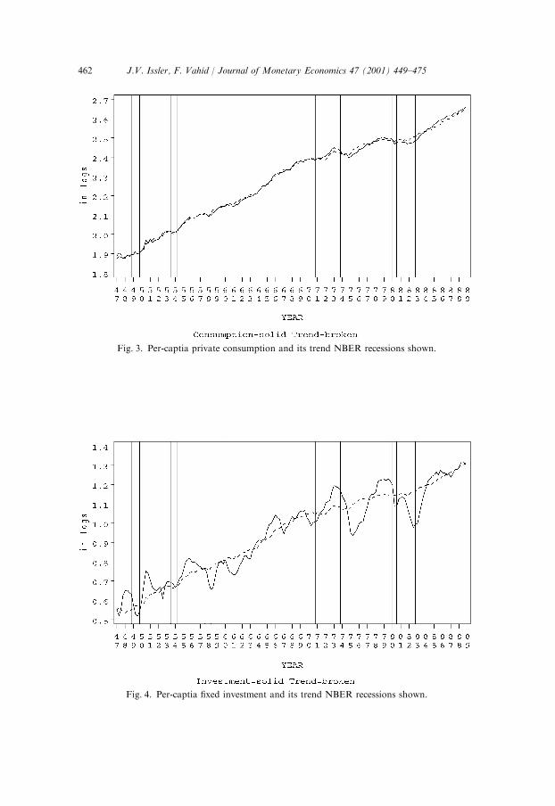
Fig. 3. Per-captia private consumption and its trend NBER recessions shown.

Fig. 4. Per-captia fixed investment and its trend NBER recessions shown.

J.V. Issler, F. Vahid / Journal of Monetary Economics 47 (2001) 449–475462

Nelson and Plosser find this issue important because they associate trends topermanent factors influencing outputFsuch as productivity, and cycles totransitory factorsFsuch as monetary policy.Since the trend-innovation effects are permanent while the cycle-innovation

effects are only transitory, it seems reasonable to attach importance to thetrend component if the trend innovation explains a significant proportion oftotal forecast errors at business-cycle horizons. The results of the variancedecomposition of output, consumption and investment are presented in Table4. This table shows the percentage of the variance of total forecast errorsexplained by permanent shocks at different horizons.11 For output, transitoryshocks explain about 50% of the forecast error variance (FEV) at the 2-yearhorizon, more than 40% at the 3-year horizon, and about 35% at the 4-yearhorizon. For shorter horizons, transitory shocks explain more than half of the

Fig. 5. Cycle in per-captia private GNP NBER recessions shown.

11For the one-quarter horizon, trend innovations are the first differences of the common trend,

while cyclical innovations are the residuals obtained by regressing cycles on the right-hand side

variables in the VECM (the lagged error-correction terms and the eight first lags of the dependent

variables). For longer horizons, we accumulate trend shocks to get trend innovations and use

higher lags of the information set to obtain the cyclical innovations. See Appendices A–C for

further details of the orthogonalization procedure.

J.V. Issler, F. Vahid / Journal of Monetary Economics 47 (2001) 449–475 463

Fig. 6. Cycle in per-capita private consumption NBER recessions shown.

Fig. 7. Cycle in per-capita fixed investment NBER recessions shown.

J.V. Issler, F. Vahid / Journal of Monetary Economics 47 (2001) 449–475464

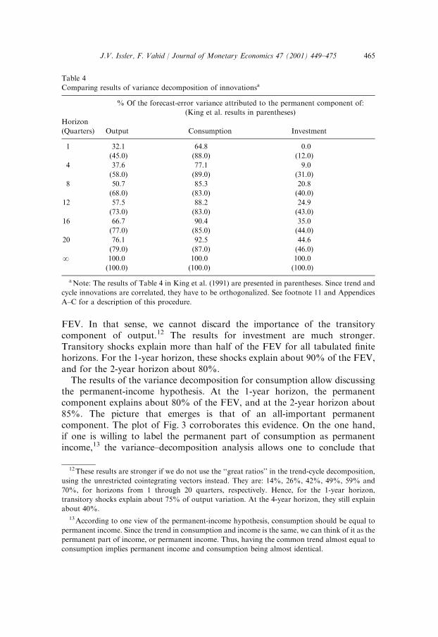
FEV. In that sense, we cannot discard the importance of the transitorycomponent of output.12 The results for investment are much stronger.Transitory shocks explain more than half of the FEV for all tabulated finitehorizons. For the 1-year horizon, these shocks explain about 90% of the FEV,and for the 2-year horizon about 80%.The results of the variance decomposition for consumption allow discussing

the permanent-income hypothesis. At the 1-year horizon, the permanentcomponent explains about 80% of the FEV, and at the 2-year horizon about85%. The picture that emerges is that of an all-important permanentcomponent. The plot of Fig. 3 corroborates this evidence. On the one hand,if one is willing to label the permanent part of consumption as permanentincome,13 the variance–decomposition analysis allows one to conclude that

Table 4

Comparing results of variance decomposition of innovationsa

% Of the forecast-error variance attributed to the permanent component of:

(King et al. results in parentheses)

Horizon

(Quarters) Output Consumption Investment

1 32.1 64.8 0.0

(45.0) (88.0) (12.0)

4 37.6 77.1 9.0

(58.0) (89.0) (31.0)

8 50.7 85.3 20.8

(68.0) (83.0) (40.0)

12 57.5 88.2 24.9

(73.0) (83.0) (43.0)

16 66.7 90.4 35.0

(77.0) (85.0) (44.0)

20 76.1 92.5 44.6

(79.0) (87.0) (46.0)

N 100.0 100.0 100.0

(100.0) (100.0) (100.0)

aNote: The results of Table 4 in King et al. (1991) are presented in parentheses. Since trend and

cycle innovations are correlated, they have to be orthogonalized. See footnote 11 and Appendices

A–C for a description of this procedure.

12These results are stronger if we do not use the ‘‘great ratios’’ in the trend-cycle decomposition,

using the unrestricted cointegrating vectors instead. They are: 14%, 26%, 42%, 49%, 59% and

70%, for horizons from 1 through 20 quarters, respectively. Hence, for the 1-year horizon,

transitory shocks explain about 75% of output variation. At the 4-year horizon, they still explain

about 40%.13According to one view of the permanent-income hypothesis, consumption should be equal to

permanent income. Since the trend in consumption and income is the same, we can think of it as the

permanent part of income, or permanent income. Thus, having the common trend almost equal to

consumption implies permanent income and consumption being almost identical.

J.V. Issler, F. Vahid / Journal of Monetary Economics 47 (2001) 449–475 465

permanent income is by far the most important component of consumption.Moreover, consumption and permanent income obey long-run proportionality,an important theoretical result. On the other, although we found excesssensitivity in consumption, e.g., Hall (1978) and Flavin (1981), consumption’stransitory part has very little importance.At this point, it is useful to compare the result of our variance decomposition

with those of King et al. (1991). Since both studies used the same data andsample period, the results are directly comparable and any differences in resultscan be attributed to short-run co-movement restrictions being imposed by ourmethod. King et al. results are reported in parentheses in Table 4. As expected,the major differences in results occur for short horizons (1–12 quarters): theirmethod under-estimates the contribution of the transitory portion of outputand investment. The same happens for consumption for the 1-to-4-quarterhorizon, being reversed, however, for longer horizons. The biggest discrepancyhappens for output: in their method, the permanent portion of output explainsalmost 60% (70%) of output variance for the 1-(2-)year horizon, whereas ourresult assigns about 40% (50%) to it. These differences are enough to changethe emphasis of the variance decomposition results for output. It is clear that amuch more considerable role should be attributed to sources of transitorynoise. It is important to note that this result was obtained in a frameworkwhere only real variables were considered, which in itself potentially limits therole of some sources of transitory shocks, e.g., monetary policy; see the resultsin King et al. (1991) when monetary variables are included in the VAR and alsothe discussion in Hansen and Heckman (1996, footnote 9).The importance of transitory components of output was also reported by

Cochrane (1994), and a similar general result is achieved by King et al. (1991),after augmenting their VAR with monetary-sector variables. More recently,Galı́ (1999) has shown that nominal (non-permanent) shocks are critical forexplaining the conditional correlation pattern of labor productivity andemployment (or hours). Moreover, these nominal shocks are responsible forthe synchronized cyclical behavior of GDP and hours: when the nominal-shockcomponents of GDP and hours are ignored, these two series fail to show anydistinct business-cycle pattern (see Galı́’s Fig. 6, p. 268). Along the same lines,den Haan (1996) finds that output and prices are positively correlated atbusiness-cycle horizons, although negatively correlated in the long run. Thissupports the conclusion that nominal shocks are important in the short runwhile real shocks are important in the long run. It also illustrates that thehorizon matters for investigating the plausibility of different theories, a pointalso stressed by Hansen and Heckman (1996).This body of evidence goes against the claim in Nelson and Plosser (1982)

that permanent shocks are the most important source of variation for output.Although there is no doubt that this is true for long horizons, results forbusiness-cycle horizons point towards the importance of transitory shocks. If

J.V. Issler, F. Vahid / Journal of Monetary Economics 47 (2001) 449–475466

the horizon matters, it would be interesting to consider the most precisetechnique at short horizons, and this is exactly what we have tried to provide inthis paper.Although it seems that our and more recent results show the importance of

nominal shocks at business-cycle horizons, it is not obvious how to interpretthe evidence. Theoretical models are rarely built in terms of permanent ortransitory shocks. Rather, they are built in terms of real (e.g., productivity) ornominal (e.g., monetary) shocks. Thus, to test theories, one has usually toimpose identifying assumptions. For example, Blanchard and Quah (1989),King et al. (tri-variate system), and Galı́ assume that the only source ofpermanent shocks is productivity. Non-permanent shocks are labelled‘‘demand’’ shocks by Blanchard and Quah and Galı́. However, one cancertainly think of permanent demand shocks (a permanent change inpreferences, for example) or of transitory supply shocks (transitorytechnology shocks, for example). In these cases those identifying assumptionswill fail.14

Although answering these issues is out of the scope of this paper, we arguethat the results here and elsewhere are still useful. We rely on the reasonableassumption that permanent shocks are more likely to be real, whereastransitory shocks are more likely to be nominal. This ‘‘axiom,’’ as far as weknow, has never been openly challenged, despite the fact that more than 17years have now elapsed since Nelson and Plosser first used it.

4.1. Post-sample forecasts of per-capita output, consumption and investment

This last section compares post-sample forecasts of two econometricrepresentations of our tri-variate system. The first is the unrestricted VECM(UVECM), which does not take into account short-run restrictions implied bythe existence of common cycles; see (A.5). The second is the restrictedVECM (RVECM), which takes those restrictions into account; see (A.6).Sample estimates used data for output, consumption, and investment from1947:1 to 1988:4. Post-sample one-step-ahead forecasts for each representationwere then calculated from 1989:1 to 1994:2, comprising 22 quarterlyobservations.Estimation of the UVECM used eight lags for all lagged dependent variables

and one lag for the error-correction terms. Since it is a reduced-form, it wasestimated by least squares. The RVECM was estimated using the same lagstructure as the UVECM, but imposing common-cycle restrictions on thesystem. As discussed in Appendices A–C, these restrictions can be conveniently

14This, however, is not the only problem. In an economy with distortions, Basu and Fernald

(1997) show that there are many sources of productivity variation unrelated to technology, which

raises the issue of what is really being ‘‘identified’’ by the literature.

J.V. Issler, F. Vahid / Journal of Monetary Economics 47 (2001) 449–475 467

formulated in terms of exclusion restrictions in a system of ‘‘structural’’ 15

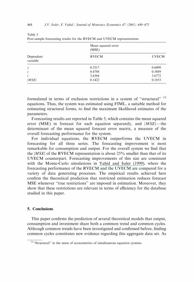
equations. Thus, the system was estimated using FIML, a suitable method forestimating structural forms, to find the maximum likelihood estimates of theparameters.Forecasting results are reported in Table 5, which contains the mean squared

error (MSE) in forecast for each equation separately, and jMSEjFthedeterminant of the mean squared forecast error matrix, a measure of theoverall forecasting performance for the system.For individual equations, the RVECM outperforms the UVECM in

forecasting for all three series. The forecasting improvement is mostremarkable for consumption and output. For the overall system we find thatthe jMSEj of the RVECM representation is about 25% smaller than that of itsUVECM counterpart. Forecasting improvements of this size are consistentwith the Monte-Carlo simulations in Vahid and Issler (1999), where theforecasting performance of the RVECM and the UVECM are compared for avariety of data generating processes. The empirical results achieved hereconfirm the theoretical prediction that restricted estimation reduces forecastMSE whenever ‘‘true restrictions’’ are imposed in estimation. Moreover, theyshow that these restrictions are relevant in terms of efficiency for the databasestudied in this paper.

5. Conclusions

This paper confirms the prediction of several theoretical models that output,consumption and investment share both a common trend and common cycles.Although common trends have been investigated and confirmed before, findingcommon cycles constitutes new evidence regarding this aggregate data set. As

Table 5

Post-sample forecasting results for the RVECM and UVECM representations

Mean squared error

(MSE)

Dependent RVECM UVECM

variable

y 0.5317 0.6099

c 0.4788 0.5889

i 3.6384 3.6772

jMSEj 0.1422 0.1853

15 ‘‘Structural’’ in the sense of econometrics of simultaneous equation systems.

J.V. Issler, F. Vahid / Journal of Monetary Economics 47 (2001) 449–475468

discussed above, this finding is relevant for calculating more precisely therelative importance of permanent and transitory shocks at business-cyclehorizons, for which this issue is still controversial and which economic agentsfind more relevant for welfare considerations.The results show that transitory shocks are more important than previously

thought. They explain about 50% of the variation of output at the 2-yearhorizon, about 40% at the 3-year horizon, and about 35% at the 4-yearhorizon. The results for investment are even stronger: more than 90% for the 1-year horizon, about 80% for the 2-year horizon, and more than 50% at the 5-year horizon. Despite these results, the permanent shock explains a very largeproportion of consumption variation, providing evidence of consumptionsmoothing over time. The importance of transitory shocks documented herefinds support in the recent research by Galı́ (1999) and den Haan (1996), as wellas in the work of Cochrane (1994). It may be a sign that nominal shocks arerelevant for the short-run variations of macroeconomic data.Finally, by using a post-sample forecasting exercise, this paper establishes

that ignoring common-cycle restrictions in this multivariate data set can lead toa non-trivial loss of efficiency in estimating reduced-form VECM’s. This canaffect the precision of estimates of trends and cycles, as well as the precision ofimpulse–response and variance–decomposition exercises. Therefore, testing forcommon cycles should always precede econometric estimation whenever short-run co-movement restrictions are likely to be present.

Appendix A. Co-movement restrictions in dynamic models

Before discussing the dynamic representation of the data, and the trend-cycledecomposition method we have used, we present the definitions of commontrends and common cycles. For a full discussion see Engle and Granger (1987)and Vahid and Engle (1993), respectively. First, we assume that yt is a n-vectorof Ið1Þ variables, with the stationary ðMAðNÞÞ Wold representation given by

Dyt ¼ CðLÞet; ðA:1Þ

where CðLÞ is a matrix polynomial in the lag operator, L, with Cð0Þ ¼ In,PN

j¼1 jjCj jjoN . The vector et is a n 1 vector of stationary one-step-aheadlinear forecast errors in yt; given information on the lagged values of yt. We canrewrite Eq. (A.1) as

Dyt ¼ Cð1Þet þ DC * ðLÞet; ðA:2Þ

where C *i ¼

Pj>i @Cj for all i: In particular, C *

0 ¼ In@Cð1Þ.

J.V. Issler, F. Vahid / Journal of Monetary Economics 47 (2001) 449–475 469

If we integrate both sides of Eq. (A.2) we get:

yt ¼ Cð1ÞXNs¼0

et@s þ C * ðLÞet

¼Tt þ Ct: ðA:3Þ

Eq. (A.3) is the multivariate version of the Beveridge–Nelson trend-cyclerepresentation (Beveridge and Nelson, 1981). The series yt are represented assum of a random walk part Tt which is called the ‘‘trend’’ and a stationary partCt which is called the ‘‘cycle’’.

Definition A.1. The variables in yt are said to have common trends (orcointegrate) if there are r linearly independent vectors, ron, stacked in an r nmatrix a0, with the following property:16

a0rn

Cð1Þ ¼ 0:

Definition A.2. The variables in yt are said to have common cycles if there are slinearly independent vectors, spn@r, stacked in an s n matrix *a0, with theproperty that

*a0sn

C * ðLÞ ¼ 0:

Thus, cointegration and common cycles represent restrictions on theelements of Cð1Þ and C * ðLÞ, respectively.We now discuss restrictions on the dynamic autoregressive representation of

economic time series arising from cointegration (common trends) and commoncycles. First, we assume that yt is generated by a vector autoregression (VAR):

yt ¼ G1yt@1 þyþ Gpyt@p þ et: ðA:4Þ

If elements of yt cointegrate, then the matrix I@Pp

i¼1 Gi must have lessthan full rank, which imposes cross-equation restrictions on the VAR. In thiscase, Engle and Granger (1987) show that system (A.4) can be written as a

16This definition could alternatively be expressed in terms of an n r matrix g, such that

Cð1Þg ¼ 0:

The Granger-representation theorem (Engle and Granger, 1987) shows that if the series in yt are

cointegrated, a and g in Eq. (A.5) satisfy:

Cð1Þg ¼ 0;

and

a0Cð1Þ ¼ 0:

J.V. Issler, F. Vahid / Journal of Monetary Economics 47 (2001) 449–475470

vector error-correction model (VECM):

Dyt ¼ G*1 Dyt@1 þyþ G*

p@1 Dyt@pþ1 þ ga0yt@1 þ et; ðA:5Þ

where g and a are full rank matrices of order n r, r is the rank of thecointegrating space, @ðI@

Ppi¼1 GiÞ ¼ ga0, and G*

j ¼ @Pp

i¼jþ1 Gi,j ¼ 1;y; p@1. Given the cointegrating vectors stacked in a0, it can be seenthat (A.5) parsimoniously encompasses (A.4). Conditional on knowledge ofcointegrating vectors, the VECM has n2ðp@1Þ þ nr parameters in theconditional mean, while the VAR has n2p parameters. Thus, the former hasnðn@rÞ fewer parameters, since ron. If we take into account the freeparameters in the cointegrating vector, the VECM has n2ðp@1Þ þ 2nr@r2

mean parameters, ðn@rÞ2 fewer than the VAR.Vahid and Engle (1993) show that the dynamic representation of the data yt

may have additional cross-equation restrictions if there are common cycles. Tosee this, recall that the cofeature vectors *a0i, stacked in an s n matrix *a0,eliminate all serial correlation in Dyt; i.e. *a0Dyt ¼ *a0et. Since the cofeaturevectors are identified only up to an invertible transformation, we can, withoutloss of generality, rotate *a to have an s dimensional identity sub-matrix:

*a ¼Is

*a*ðn@sÞs

" #:

Considering *a0Dyt ¼ *a0et as s equations in a system, and completing the systemby adding the unconstrained VECM equations for the remaining n@selements of Dyt; we obtain,

Is *a*0

0ðn@sÞs In@s

" #Dyt ¼

0sðnpþrÞ

G* *1 yG* *

p@1g*

" # Dyt@1

^

Dyt@pþ1

a0yt@1

26664

37775þ vt; ðA:6Þ

where G* *i and g* represent the partitions of G*

i and g, respectively,corresponding to the bottom n@s reduced form VECM equations, and

vt ¼Is *a*

0

0ðn@sÞs In@s

" #et:

It is easy to show that (A.6) parsimoniously encompasses (A.5). Since

Is *a*0

0ðn@sÞs In@s

" #

is invertible, it is possible to recover (A.5) from (A.6). Notice, however, that thelatter has sðnpþ rÞ@sðn@sÞ fewer parameters.

J.V. Issler, F. Vahid / Journal of Monetary Economics 47 (2001) 449–475 471

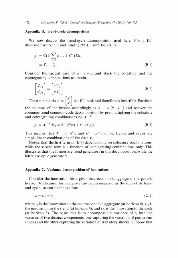
Appendix B. Trend-cycle decomposition

We now discuss the trend-cycle decomposition used here. For a fulldiscussion see Vahid and Engle (1993). From Eq. (A.3):

yt ¼ Cð1ÞXNs¼0

et@s þ C * ðLÞet

¼ Tt þ Ct: ðB:1Þ

Consider the special case of n ¼ rþ s; and stack the cofeature and thecointegrating combinations to obtain,

*a0yta0yt

" #¼

*a0Tt

a0Ct

" #: ðB:2Þ

The n nmatrix A ¼*a0

a0

�has full rank and therefore is invertible. Partition

the columns of the inverse accordingly as A@1 ¼ ½*a@a@� and recover thecommon-trend common-cycle decomposition by pre-multiplying the cofeatureand cointegrating combinations by A@1:

yt ¼ A@1Ayt ¼ *a@ð*a0ytÞ þ a@ða0ytÞ: ðB:3Þ

This implies that Tt ¼ *a@ *a0yt and Ct ¼ a@a0yt, i.e. trends and cycles aresimple linear combinations of the data yt.Notice that the first term in (B.3) depends only on cofeature combinations,

while the second term is a function of cointegrating combinations only. Thisillustrates that the former are trend generators in this decomposition, while thelatter are cycle generators.

Appendix C. Variance decomposition of innovations

Consider the innovation for a given macroeconomic aggregate, at a generichorizon h. Because this aggregate can be decomposed as the sum of its trendand cycle, so can its innovations:

et ¼ e1t þ e2t; ðC:1Þ

where et is the innovation to the macroeconomic aggregate (at horizon h), e1t isthe innovation to the trend (at horizon h), and e2t is the innovation to the cycle(at horizon h). The basic idea is to decompose the variance of et into thevariance of two distinct components: one capturing the variation of permanentshocks and the other capturing the variation of transitory shocks. Suppose that

J.V. Issler, F. Vahid / Journal of Monetary Economics 47 (2001) 449–475472

ðe1t; e2tÞ0 has the following structure:

e1te2t

!B 0;

s11 s12s12 s22

! !:

Because in general these two innovations are correlated, i.e., s12a0, to performthe variance decomposition of et we have to orthogonalize e1t and e2t. Considerusing the following reparameterization:

m1t ¼ 1þs12s11

� �e1t

and

m2t ¼ e2t@s12s11

e1t:

We label m1t as the innovation to the permanent component (at horizon h), andm2t as the innovation to the transitory component (at horizon h).17 Adding andsubtracting ðs12=s11Þe1t to (C.1) shows that

et ¼ e1t þ e2t þs12s11

e1t@s12s11

e1t

¼ e1t þs12s11

e1t

� �þ e2t@

s12s11

e1t

� �

¼ m1t þ m2t

and that,

E½m1tm2t� ¼ 1þs12s11

� �E½e1tm2t�

¼ 1þs12s11

� �s12@

s12s11

s11

� �¼ 0;

i.e., that the m’s are orthogonal. Hence,

VARðetÞ ¼ VARðm1t þ m2tÞ ¼ VARðm1tÞ þ VARðm2tÞ

¼ 1þs12s11

� �2

s11

" #þ s22@

s212s11

�;

which allows decomposing the variance of et into that of two orthogonalcomponents: m1t and m2t.

17Notice that m2t is just the residual of the regression of e2t on e1t, so it makes sense to label it theinnovation to the transitory component.

J.V. Issler, F. Vahid / Journal of Monetary Economics 47 (2001) 449–475 473

References

Basu, S., Fernald, J., 1997. Aggregate productivity and aggregate technology. Working Paper,

University of Michigan.

Beveridge, S., Nelson, C.R., 1981. A new approach to decomposition of economic time series into a

permanent and transitory components with particular attention to measurement of the business

cycle. Journal of Monetary Economics 7, 151–174.

Blanchard, O.J., Quah, D., 1989. The dynamic effects of aggregate supply and demand

disturbances. American Economic Review 79, 655–673.

Campbell, J.Y., 1987. Does saving anticipate declining labor income? An alternative test of the

permanent income hypothesis. Econometrica 55 (6), 1249–1273.

Campbell, J.Y., Mankiw, N.G., 1987. Permanent and transitory components in macroeconomic

fluctuations. American Economic Review.

Campbell, J.Y., Mankiw, N.G., 1989. Consumption, income and interest rates: reinterpreting the

time series evidence. NBER Macroeconomics Annual.

Cochrane, J.H., 1988. How big is the random walk in GNP? Journal of Political Economy 96, 893–

920.

Cochrane, J.H., 1994. Permanent and transitory components of GNP and stock prices. Quarterly

Journal of Economics 30, 241–265.

den Haan, W., 1996. The comovements between real activity and prices at different business cycle

frequencies. Working Paper, University of California, San Diego.

Engle, R.F., Granger, C.W.J., 1987. Cointegration and error correction: representation, estimation

and testing. Econometrica 55, 251–276.

Engle, R.F., Issler, J.V., 1995. Estimating common sectoral cycles. Journal of Monetary Economics

35, 83–113.

Engle, R.F., Kozicki, S., 1993. Testing for common features. Journal of Business and Economic

Statistics 11, 369–395.

Engle, R.F., Yoo, B.S., 1987. Forecasting and testing in cointegrated systems. Journal of

Econometrics 35, 143–159.

Fama, E., 1992. Transitory variation in investment and output. Journal of Monetary Economics

30, 467–480.

Flavin, M.A., 1981. The adjustment of consumption to changing expectation about future income.

Journal of Political Economy 89 (5), 974–1009.

Galı́, J., 1999. Technology, employment and the business cycle: do technology shocks explain

aggregate fluctuations? American Economic Review 77 (2), 111–117.

Gonzalo, J., Ng, S., 1999. A systematic approach for analyzing the dynamic effects of permanent

and transitory shocks. Working Paper, Universidad Carlos III de Madrid.

Hall, R.E., 1978. Stochastic implications of the Life cycle-permanent income hypothesis: theory

and evidence. Journal of Political Economy 86, 971–987.

Hansen, L.P., Heckman, J.J., 1996. The empirical foundations of calibration. Journal of Economic

Perspectives 10 (1), 87–104.

Johansen, S., 1988. Statistical analysis of cointegrating vectors. Journal of Economic Dynamics and

Control 12, 231–254.

Johansen, S., 1991. Estimation and hypothesis testing of cointegration vectors in Gaussian vector

autoregressive models. Econometrica 59, 1551–1580.

King, R.G., Plosser, C.I., Rebelo, S., 1988. Production, growth and business cycles. II. New

directions. Journal of Monetary Economics 21, 309–341.

King, R.G., Plosser, C.I., Stock, J.H., Watson, M.W., 1991. Stochastic trends and economic

fluctuations. American Economic Review 81, 819–840.

Kosobud, R., Klein, L., 1961. Some econometrics of growth: great ratios of economics. Quarterly

Journal of Economics 25, 173–198.

J.V. Issler, F. Vahid / Journal of Monetary Economics 47 (2001) 449–475474

Lucas, R.E. Jr., 1977. Understanding business cycles. Carnegie-Rochester Conference Series on

Public Policy, Vol. 5. North Holland, Amsterdam, pp. 7–29.

Nelson, C.R., Plosser, C.I., 1982. Trends and random walks in macroeconomic time series. Journal

of Monetary Economics 10, 139–162.

Osterwald-Lenum, M., 1992. Quantiles of the asymptotic distribution of the maximum likelihood

cointegration rank test statistics. Oxford Bulletin of Economics and Statistics 54, 461–472.

Rao, C.R., 1973. Linear Statistical Inference.. Wiley, New York.

Romer, P., 1986. Increasing returns and long run growth. Journal of Political Economy 94, 1002–

1037.

Vahid, F., Engle, R.F., 1993. Common trends and common cycles. Journal of Applied

Econometrics 8, 341–360.

Vahid, F., Engle, R.F., 1997. Codependent cycles. Journal of Econometrics 80, 199–211.

Vahid, F., Issler, J.V., 1999. The importance of common-cyclical features in VAR analysis: a

Monte–Carlo study. Working Paper: Getulio Vargas Foundation and Monash University.

Watson, M.W., 1986. Univariate detrending methods with stochastic trends. Journal of Monetary

Economics 18, 49–75.

J.V. Issler, F. Vahid / Journal of Monetary Economics 47 (2001) 449–475 475