Combining the Tactile Resonance Method and Raman ...
150
DOCTORAL THESIS Combining the Tactile Resonance Method and Raman Spectroscopy for Tissue Characterization towards Prostate Cancer Detection Stefan Candefjord 500 μm Young’s modulus (kPa) 20 40 60 80 100 120
-
Upload
khangminh22 -
Category
Documents
-
view
1 -
download
0
Transcript of Combining the Tactile Resonance Method and Raman ...
DOCTORA L T H E S I S
Department of Computer Science, Electrical and Space EngineeringDivision of Systems and InteractionBiomedical Engineering Laboratory
Combining the Tactile Resonance Method and Raman Spectroscopy for
Tissue Characterization towards Prostate Cancer Detection
Stefan Candefjord
ISSN: 1402-1544 ISBN 978-91-7439-252-4
Luleå University of Technology 2011
Stefan Candefjord C
ombining the T
actile Resonance M
ethod and Ram
an Spectroscopy for Tissue C
haracterization towards Prostate C
ancer Detection
ISSN: 1402-1544 ISBN 978-91-7439-XXX-X Se i listan och fyll i siffror där kryssen är
500µm
You
ng’smodulus(kPa)
20
40
60
80
100
120


Combining the Tactile ResonanceMethod and Raman Spectroscopy
for Tissue Characterization towardsProstate Cancer Detection
Stefan Candefjord
Dept. of Computer Science, Electrical and Space EngineeringLulea University of Technology
Lulea, Sweden

Printed by Universitetstryckeriet, Luleå 2011
ISSN: 1402-1544 ISBN 978-91-7439-252-4
Luleå 2011
www.ltu.se

To the memory of my father, Jan-Ake Candefjord
iii

iv
Abstract
Prostate cancer (PCa) is the most common male cancer in Europe and the US, and onlylung and colorectal cancer have a higher mortality among European men. In Sweden,PCa is the most common cause of cancer-related death for men.
The overall aim of this thesis was to explore the need for new and complementarymethods for PCa detection and to take the first step towards a novel approach: combiningthe tactile resonance method (TRM) and Raman spectroscopy (RS). First, the mainmethods for PCa detection were reviewed. Second, to establish a robust protocol for RSexperiments in vitro, the effects of snap-freezing and laser illumination on porcine prostatetissue were studied using RS and multivariate statistics. Third, measurements on porcineand human tissue were performed to compare the TRM and RS data via multivariatetechniques, and to assess the accuracy of classifying healthy and cancerous tissue using asupport vector machine algorithm.
It was concluded through the literature review that the gold standard for PCa detectionand diagnosis, the prostate specific antigen test and systematic biopsy, have low sensitivityand specificity. Indolent and aggressive tumors cannot be reliably differentiated, andmany men are therefore treated either unnecessarily or too late. Clinical benefits ofthe state–of–the–art in PCa imaging – advanced ultrasound and MR techniques – havestill not been convincingly shown. There is a need for complementary and cost-effectivedetection methods. TRM and RS are promising techniques, but hitherto their potentialfor PCa detection have only been investigated in vitro.
In the RS study no evidence of tissue degradation due to 830 nm laser illumination atan irradiance of ∼ 3 · 1010 W m−2 were found. Snap-freezing and subsequent storage at−80 ◦C gave rise to subtle but significant changes in Raman spectra, most likely relatedto alterations in the protein structure. The major changes due to PCa do not seem to berelated to the protein structure, hence snap-freezing may be applied in our experiments.
The combined measurements on porcine and human prostate tissue showed that RSprovided additional discriminatory power to TRM. The classification accuracy for healthyporcine prostate tissue, and for healthy and cancerous human prostate tissue, was > 73%.This shows the power of the support vector machine applied to the combined data.
In summary, this work indicates that an instrument combining TRM and RS is apromising complementary method for PCa detection. Snap-freezing of samples may beused in future RS studies of PCa. A combined instrument could be used for tumor-borderdemarcation during surgery, and potentially for guiding prostate biopsies towards lesionssuspicious for cancer. All of this should provide a more secure diagnosis and consequentlymore efficient treatment of the patient.
v

vi

ContentsPart I 1
Chapter 1 – Original Papers and My Contributions 3
Chapter 2 – Other Publications of Relevance 5
Chapter 3 – Abbreviations 7
Chapter 4 – Introduction 94.1 General background . . . . . . . . . . . . . . . . . . . . . . . . . . . . . . 94.2 The prostate . . . . . . . . . . . . . . . . . . . . . . . . . . . . . . . . . . 114.3 Tactile resonance method . . . . . . . . . . . . . . . . . . . . . . . . . . . 154.4 Raman spectroscopy . . . . . . . . . . . . . . . . . . . . . . . . . . . . . 194.5 Tissue preparation and measurement procedures . . . . . . . . . . . . . . 264.6 Mathematical tools for analysis and classification . . . . . . . . . . . . . 28
Chapter 5 – Aims 31
Chapter 6 – Material and Methods 336.1 Literature review . . . . . . . . . . . . . . . . . . . . . . . . . . . . . . . 336.2 Experimental setup . . . . . . . . . . . . . . . . . . . . . . . . . . . . . . 346.3 Sample preparation . . . . . . . . . . . . . . . . . . . . . . . . . . . . . . 386.4 Measurement procedure . . . . . . . . . . . . . . . . . . . . . . . . . . . 396.5 Data analysis and statistics . . . . . . . . . . . . . . . . . . . . . . . . . 40
Chapter 7 – General Results and Discussion 437.1 Literature review . . . . . . . . . . . . . . . . . . . . . . . . . . . . . . . 437.2 Effects of snap-freezing and laser illumination . . . . . . . . . . . . . . . 447.3 Comparing TRM and RS information . . . . . . . . . . . . . . . . . . . . 477.4 Classification of prostate tissue . . . . . . . . . . . . . . . . . . . . . . . 50
Chapter 8 – General Summary and Conclusions 55
Chapter 9 – Future Outlook 57
References 59
vii
Part II 71
Paper A – Technologies for localization and diagnosis of prostatecancer 73
Paper B – Effects of snap-freezing and near-infrared laser illumi-nation on porcine prostate tissue as measured by Raman spectro-scopy 95
Paper C – Combining fibre optic Raman spectroscopy and tactileresonance measurement for tissue characterization 105
Paper D – Combining scanning haptic microscopy and fiber opticRaman spectroscopy for tissue characterization 1151 Introduction . . . . . . . . . . . . . . . . . . . . . . . . . . . . . . . . . . 1182 Material and Methods . . . . . . . . . . . . . . . . . . . . . . . . . . . . 1193 Results . . . . . . . . . . . . . . . . . . . . . . . . . . . . . . . . . . . . . 1254 Discussion . . . . . . . . . . . . . . . . . . . . . . . . . . . . . . . . . . . 1305 Conclusion . . . . . . . . . . . . . . . . . . . . . . . . . . . . . . . . . . . 133References . . . . . . . . . . . . . . . . . . . . . . . . . . . . . . . . . . . . . . 133
viii

Acknowledgments
I would like to express my gratitude to the people who contributed to this work andsupported me during this time:
� I am most grateful to my supervisor Prof. Olof Lindahl and my co-supervisorDr. Kerstin Ramser. Thank you for giving me the opportunity to work in thisinteresting field. You have given me great guidance in research questions, and alwaysbelieved in me and encouraged me during difficult times. You have created a verygood working environment with a positive atmosphere. I think of you not only asmy supervisors, but also as my friends.
� Morgan Nyberg for all the fun and interesting work we have done together.
� The other members of the Biomedical Engineering group at Lulea University ofTechnology: Dr. Josef Hallberg, Nazanin Bitaraf and Ahmed Alrifaiy.
� Dr. Ville Jalkanen at Umea University for the collaboration and most valuableadvice.
� Dr. Yoshinobu Murayama: it has been very fun and stimulating to work with you,and I wish to continue our collaboration under new forms.
� Prof. Kerstin Vannman for valuable discussions.
� Bertil Funck and Mats Gustavsson for helping me obtaining porcine prostate samples.
� Kerstin Lofquist and Kerstin Stenberg at the Dept. of Pathology and Cytology atSunderby Hospital, and Pernilla Andersson and Birgitta Ekblom at the pathologyunit at Norrland’s University Hospital, for helping with the preparation of prostatespecimens.
� Prof. Anders Bergh at Norrland’s University Hospital for the collaboration andvaluable discussions.
� Dr. Josefine Enman, Magnus Sjoblom, Jonas Helmerius, Dr. Christian Anderssonand Maine Ranheimer at the Dept. of Chemical Engineering and Geosciences for allgood advice and giving me access to your laboratory.
ix

� All my friends and colleagues at the Dept. of Computer Science, Electrical andSpace Engineering. You have made my time as doctoral student very amusing. Ihave laughed for days after many of our discussions during coffee breaks. Manyof you have also contributed with valuable discussions and collaborative work indifferent courses. I would especially like to thank Johan Borg for all valuable tipsabout performing measurements and developing the experimental setup.
� The EU Objective 2, Northern Sweden, for supporting my work, and the KempeFoundation for funding much of our laboratory equipment.
� The study was performed within the CMTF network.
� My warmest thanks to my family and my girlfriend, Linda, for all your love andsupport.
Lulea, May 9, 2011Stefan Candefjord
x

Part I
1

2

Chapter 1
Original Papers and MyContributions
In this thesis the following peer-reviewed papers are included and referred to by theirLatin letters. My contributions to these papers are shown in Table 1.1.
(A) S. Candefjord, K. Ramser & O. A. Lindahl, “Technologies for localization anddiagnosis of prostate cancer”, Journal of Medical Engineering & Technology, vol. 33,pp. 585–603, 2009.
(B) S. Candefjord, K. Ramser & O. A. Lindahl, “Effects of snap-freezing and near-infrared laser illumination on porcine prostate tissue as measured by Ramanspectroscopy”, Analyst, vol. 134, pp. 1815–1821, 2009.
(C) S. Candefjord, M. Nyberg, V. Jalkanen, K. Ramser & O. A. Lindahl, “Combin-ing fibre optic Raman spectroscopy and tactile resonance measurement for tissuecharacterization”, Measurement Science & Technology, vol. 21, 125801 (8 pp.), 2010.
(D) S. Candefjord, Y. Murayama, M. Nyberg, J. Hallberg, K. Ramser, B. Ljungberg,A. Bergh & O. A. Lindahl, “Combining scanning haptic microscopy and fiber opticRaman spectroscopy for tissue characterization”, Submitted to Medical & BiologicalEngineering & Computing, May 2011.
Table 1.1: The contributions made by Stefan Candefjord to Papers A–D. 1 = main responsibility,2 = Contributed to high extent, 3 = Contributed.
Part A B C D
Idea and formulation of the study 2 3 2 2Experimental design - 1 2 2Performance of experiments - 1 2 1Data analysis 1 1 2 1Writing of manuscript 1 1 1 1
3

4 Original Papers and My Contributions

Chapter 2
Other Publications of Relevance
Other publications of relevance, but not included in this thesis, are listed below.
(1) S. Candefjord, “Combining a resonance and a Raman sensor: towards a new methodfor localizing prostate tumors in vivo”, Technical Report, ISSN: 1402-1536, LuleaUniversity of Technology, Lulea, Sweden, 2007.
(2) S. Candefjord, K. Ramser and O. A. Lindahl, “Towards new sensors for cancerdetection in vivo, a handheld detector combining a fibre-optic Raman probe and aresonance sensor”, Conference Abstract, Looking Skin Deep – Clinical and TechnicalAspects of Skin Imaging, 1st workshop by Goteborg Science Centre for MolecularSkin Research, Goteborg, Sweden, 2007.
(3) S. Candefjord, K. Ramser and O. A. Lindahl, “En ny metod for att lokalisera ochdiagnostisera prostatacancer”, Conference Abstract, Medicinteknikdagarna 2007,Orebro, Sweden, 2007.
(4) S. Candefjord, K. Ramser and O. A. Lindahl, “Effects of snap-freezing and laserillumination of tissue on near-infrared Raman spectra of porcine prostate tissue”,Conference Abstract, SPEC 2008, Shedding Light on Disease: Optical Diagnosis forthe New Millennium, Sao Jose dos Campos, Sao Paulo, Brazil, 2008.
(5) S. Candefjord, M. Nyberg, V. Jalkanen, K. Ramser & O. A. Lindahl, “Evaluatingthe Use of a Raman Fiberoptic Probe in Conjunction with a Resonance Sensor forMeasuring Porcine Tissue in vitro”, O. Dossel & W. C. Schlegel (ed.), WC 2009,IFMBE Proceedings, vol. 25, no. 7, pp. 414–417, 2009.
(6) S. Candefjord, “Towards new sensors for prostate cancer detection – combiningRaman spectroscopy and resonance sensor technology”, Licentiate Thesis, ISBN978-91-86233-59-4, Lulea University of Technology, Lulea, Sweden, 2009.
(7) S. Candefjord, M. Nyberg, V. Jalkanen, K. Ramser & O. A. Lindahl, “Kombinations-instrument for detektering av prostatacancer – korrelation mellan resonanssensoroch fiberoptisk Ramanprobe”, Conference Abstract, Medicinteknikdagarna 2009,Vasteras, Sweden, 2009.
5

6 Other Publications of Relevance
(8) S. Candefjord, K. Ramser & O. A. Lindahl, “Kombinationsinstrument for detekteringav prostatacancer – matningar pa snitt av grisprostata med resonanssensor ochfiberoptisk Ramanprobe”, Conference Abstract, Medicinteknikdagarna 2010, Umea,Sweden, 2010.

Chapter 3
Abbreviations
BPH benign prostatic hyperplasiaHCA hierarchical clustering analysisMR magnetic resonanceMRI magnetic resonance imagingMRSI magnetic resonance spectroscopic imagingMTS micro tactile sensorNIR near-infraredPBS phosphate buffered salinePC principal componentPCA principal component analysisPCa prostate cancerPSA prostate-specific antigenPZT lead zirconate titanateRS Raman spectroscopySHM scanning haptic microscopySB systematic biopsySVM support vector machinesTRM tactile resonance method
7

8 Abbreviations

Chapter 4
Introduction
This chapter explains the problems prostate cancer poses to public health, describes thetheory for the tactile resonance method and Raman spectroscopy, discusses pitfalls forin vitro experiments, and gives an insight into the mathematical tools that were used inthis work.
4.1 General background
Prostate cancer (PCa) is the most common form of male cancer in the US andEurope [1,2]. From the most recent data it is estimated that PCa caused almost 90 000deaths in Europe in 2008, and only lung and colorectal cancer have a higher mortalityamong European men [1]. In the US it is the second leading cause of male death due tocancer [2], and the severity of the disease is strongly related to insurance status [3]. Theincidence of PCa is expected to increase due to the aging population [4].
PCa is often indolent, more men die with the disease than from it. Considering thelarge risks for side effects such as impotence and incontinence after radical prostatectomy,i.e. surgical removal of the prostate, active surveillance may be the best option for patientswith indolent tumors [5,6]. On the other hand, to reduce PCa mortality, patients withaggressive tumors likely to metastasize must be treated early on [6]. Current clinicaldiagnostic tests, the prostate specific antigen (PSA) test, and multiple systematic biopsy(SB), miss many tumors and cannot reliably distinguish between indolent and aggressivePCa [7, 8]. As a consequence, many men are treated either unnecessarily or too late.
The prostate is a deep-sited organ with heterogeneous structure [9, 10]; that makes itdifficult to recognize tumors using medical imaging techniques. Advanced techniques forultrasound and magnetic resonance imaging (MRI) show relatively high sensitivity forPCa detection [11,12]. However, benign lesions such as prostatitis and benign prostatichyperplasia (BPH) often give false alarms [11,12].
The major objective of PCa detection is a more precise disease characterization [13].Today, there is a lack of information for deciding whether patients that undergo radicalprostatectomy would benefit from additional therapy [14]. For high-risk patients furthertreatment with medical, radiation and/or chemotherapy may be useful [14, 15]. However,selecting appropriate patients upfront is challenging, and delaying adjuvant therapy until
9

10 Introduction
there is evidence of cancer regrowth seems to decrease survival rates [14]. One reason thatmany patients suffer from cancer recurrence is failure to remove all cancerous tissue atsurgery [16]. Positive surgical margins, i.e. cancer present on the surface of the dissectedtissue, are found in up to 40% of patients [16,17]. There is currently no accurate techniquefor analyzing the surgical margins during operation [16, 17]. Thus, it becomes challengingfor surgeons to remove all cancerous tissue while avoiding damage leading to erectiledysfunction or incontinence [16]. New complementary methods for PCa detection anddiagnosis are needed. This thesis takes the first steps towards a novel approach wheretwo experimental techniques are combined, i.e. the tactile resonance method (TRM) andRaman spectroscopy (RS).
TRM was developed to mimic palpation, i.e. to feel the stiffness of a tissue usingthe fingers, and this is performed by physicians to find tissue abnormalities [18]. Thestiffness of many organs are affected by diseases. Tumors are usually stiffer than healthytissue and can be felt as hard nodules in, e.g. breast and prostate tissue. TRM gives anobjective measure of the stiffness through frequency changes of a piezoelectric vibratingelement. Several medical applications have been introduced, including measuring thestiffness of single cells to evaluate embryo quality and increase the success-rate of in vitrofertilization [18]. TRM is promising for breast and prostate cancer detection [18]. In vitrostudies show that TRM can differentiate soft, healthy prostate tissue from PCa [19–21].However, the sensitivity is currently insufficient to distinguish between tumors andrelatively hard healthy tissue, such as sites with an accumulation of prostate stones.
RS measures the biochemical composition of tissue via laser illumination and analysisof the spectrum of the inelastically scattered light. Disease progression is reflected bychanges in the molecular contents of tissue [22]. RS is very promising for a wide range ofdiagnostic applications [22]. Numerous in vitro studies show that RS can detect manytypes of cancers, including PCa, with high sensitivity and specificity [22–27]. Despite thishigh potential, few clinical implementations have emerged. The main reason is a lack ofsmall, flexible and disposable RS fiber optic probes adequate for large clinical trials [28].RS is very promising for distinguishing indolent and aggressive PCa [24,25,27,29]. Thedisadvantages of RS are that current fiber optic probes have short penetration depth intissue (∼ 0.1 mm [30]), that surrounding light can interfere with the signal of interest,and that intense laser irradiation may damage tissue.
To combine TRM and RS could add up their strengths while minimizing the drawbacksassociated with each technique. TRM constitutes a quick, gentle and deep-sensing methodthat could be used for swift scanning of the tissue. RS could provide complementaryinformation for nodules suspected to be cancerous. In the first place, the combinedinstrument could be used to probe the surgical margins during radical prostatectomy.In the long term, it could potentially be used for minimally invasive localization anddiagnosis of PCa.
In vitro studies are necessary for successful implementation of the combined instrument.To ascertain that the results are transferable to the in vivo situation, it is importantthat the experimental procedures preserve the native tissue characteristics. Possibledegradation of tissue from, e.g. sample preservation and preparation methods, laser

4.2. The prostate 11
irradiation, and dehydration during measurements, should be investigated.This thesis gives a background to the difficulties of localizing and diagnosing PCa.
It reviews the main methods for PCa detection in clinical use today, and discussespromising novelties that are being developed. The importance of robust in vitro studyprotocols is discussed, and the effects of snap-freezing and near-infrared laser (NIR)illumination on porcine prostate tissue are investigated using RS. An approach forcombining the information from TRM and RS is developed and evaluated on measurementson porcine abdominal tissue. Finally, the accuracy of classification of healthy and cancerousprostate tissue is investigated in experiments on porcine and human samples using a novelexperimental setup with a micro tactile sensor (MTS) and an RS fiberoptic probe.
4.2 The prostate
4.2.1 Anatomy and physiology
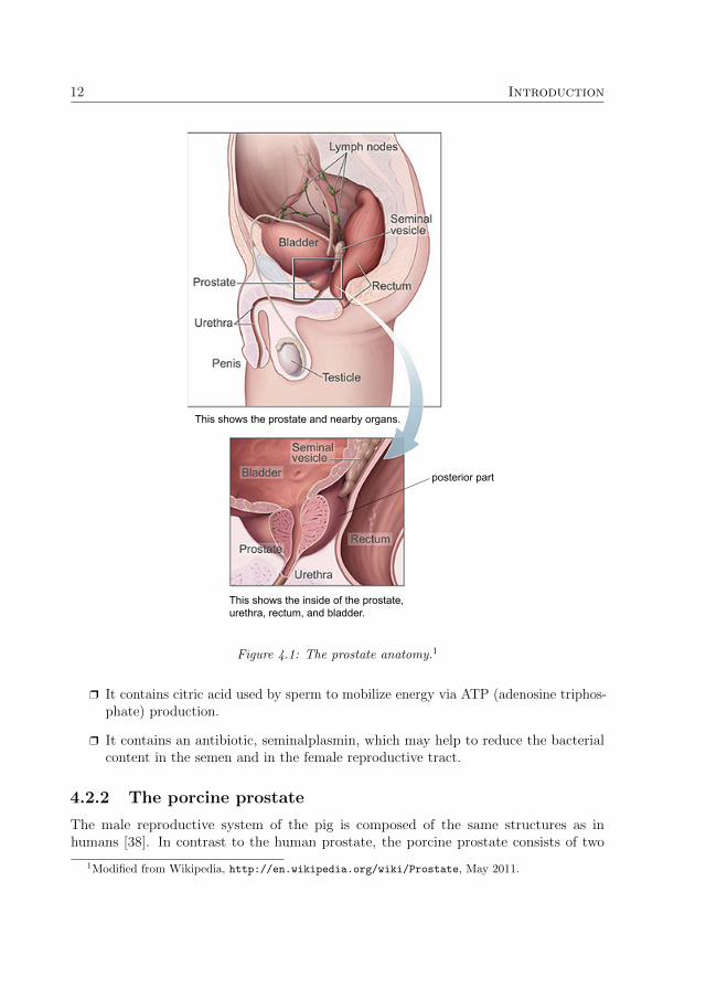
The prostate is an accessory sex gland whose function is to store and secrete a milky,slightly acidic fluid (pH ∼ 6.5), which makes up about 25% of the volume of semen [31].The gland is about the size of a golf ball and resembles a walnut in shape. It is situatedinferior to the bladder, next to the rectal wall that is about 3 mm thick [32], and encirclesthe prostatic urethra (Figure 4.1). Many prostatic ducts lead the prostatic fluid into theurethra. The prostate is composed of glandular elements that are lined with epithelial cellsthat secrete prostatic fluid into the glandular lumen (cavity) [10]. The glandular elementsare separated by stroma, a supportive framework that consists of smooth muscle tissueand other cellular components embedded in an extracellular matrix rich in collagen [31,33].There are three anatomical zones in the prostate: the peripheral zone, the transitionalzone and the central zone. The composition of the prostate tissue varies between thezones, e.g. the stroma is more or less compact with varying amounts of muscle tissue [10].
The prostate normally increases in volume during specific periods throughout a man’slife. It grows rapidly from puberty until about age 30, remains at a stable size betweenage 30 and 45, after which it may begin to grow again [31]. The majority of men > 55years develop BPH, a benign enlargement of the prostate [34]. The formation of prostatestones (corpora amylacea) in the lumen of the glandular elements, due to solidification ofglandular secretions, is another common benign occurrence [35,36]. The stones are quitehard and contribute to tissue stiffness, although they make up only a small fraction ofthe tissue volume [19,37]. They are rarely present in cancerous tissue [36].
The functional role of prostatic fluid is not completely understood, but the followingis known [31]:
r It participates in making the semen coagulate after ejaculation, which happenswithin five minutes (the role of coagulation is unknown).
r It contains protein-digesting enzymes, among them, PSA, which starts to liquefythe semen at 10–20 minutes after ejaculation. This facilitates the movement ofsperm through the cervix.
12 Introduction
posterior part
This shows the inside of the prostate,urethra, rectum, and bladder.
This shows the prostate and nearby organs.
Figure 4.1: The prostate anatomy.1
r It contains citric acid used by sperm to mobilize energy via ATP (adenosine triphos-phate) production.
r It contains an antibiotic, seminalplasmin, which may help to reduce the bacterialcontent in the semen and in the female reproductive tract.
4.2.2 The porcine prostate
The male reproductive system of the pig is composed of the same structures as inhumans [38]. In contrast to the human prostate, the porcine prostate consists of two
1Modified from Wikipedia, http://en.wikipedia.org/wiki/Prostate, May 2011.

4.2. The prostate 13
parts, compacta and disseminata [39]. The compact part appears as a number of roundedelevations on the dorsal (towards the back) side of the urethra, whereas the disseminatepart surrounds the urethra [39,40]. The two parts are histologically similar [39]. Prostatestones are present only occasionally in the boar prostate [39]. Nicaise et al. [40] used lightand electron microscopy to study the disseminate prostate of 12 boars and 8 barrows,i.e. castrated boars. The prostate of the barrows did not develop normally. The authorsconcluded that the results permitted the use of the boar prostate as an experimentalmodel for studying the influence of hormones used in human medicine.
4.2.3 Prostate cancer
In Sweden about 10 000 men are diagnosed with PCa each year and more than 2500 diefrom the disease, making it the most common cause of cancer-related male death [1].Scandinavia and the Baltic region (Estonia, Latvia and Lithuania) have the highestPCa mortality rates in Europe [41]. PCa is often without symptoms, even in men withaggressive tumors, until severe stages [42]. Estimations based on autopsies show that upto 50% of men harbor PCa by 70 years of age [42, 43]. However, the vast majority oftumors are indolent [8]. In its most aggressive form PCa disperses metastases and is verydangerous; the 5-year survival rate is only 34% [44]. In contrast, survival is 100% if thecancer has not spread beyond the structures adjacent to the prostate or metastasized todistant lymph nodes [44].
Almost all, 95%, of prostate tumors form in the prostatic ducts in the glandularepithelium [44]. The majority develop in the posterior part of the gland (the peripheralzone) [45,46], which is situated towards the rectum (Figure 4.1). PCa is usually multifocaland provides little contrast to healthy tissue using standard clinical imaging methods,such as ultrasound and MRI. This makes the cancer nodules difficult to detect [47,48].
The causes of PCa remain largely unexplained [41]. Age, ethnicity and family his-tory have been established as risk factors, and diet and genetic susceptibility may con-tribute [41].
4.2.4 Detection and diagnosis of prostate cancer
The clinical tests that are used for detection and diagnosis of PCa are the PSA test andSB. Historically, digital rectal examination, i.e. the physician palpates the prostate viathe rectum, was the most important test [49, 50]. This method has low accuracy [48] andcan usually only detect severe forms of PCa [50]. It is still used as a complement [50]. Ahigh concentration of PSA in the blood indicates cancer [51]. However, the PSA level canbe elevated also for men without PCa, often due to BPH [51], and men with normal levelsmay still have cancer [52]. A multicenter European randomized study including 182 000men found that PSA-based screening reduced the PCa mortality by 20% [8]. However, italso caused unneccessary treatments and overdiagnosis, i.e. confirming cancer in patientswith indolent tumors that would never cause clinical symptoms in their lifetime. Toprevent one death 1410 men would have to be screened and 48 additional patients wouldhave to undergo treatment. A similar study in the US, which enrolled almost 77 000 men,

14 Introduction
did not find any significant benefits of PSA screening [53]. One possible explanation forthe different outcomes is that the European study used a PSA cutoff of 3 ng mL−1 inmost centers, as compared to 4 ng mL−1 in the US study. In addition, about 50% of thepatients in the control group in the US were screened as part of usual care [53]. It hasbeen estimated that the rate of overdiagnosis due to PSA screening is 50% [54].
If PCa is suspected from elevated PSA or digital rectal examination SB is performed [50].An ultrasound probe equipped with a spring-loaded biopsy gun is inserted into the rectum,and the biopsy needle is directed to at least six predetermined sites according to the SBprotocol [50]. SB fails to detect 20–30% of present tumors [7]. This can be appreciated sincethe volume of a biopsy typically is less than one thousandth of the prostate volume [55].
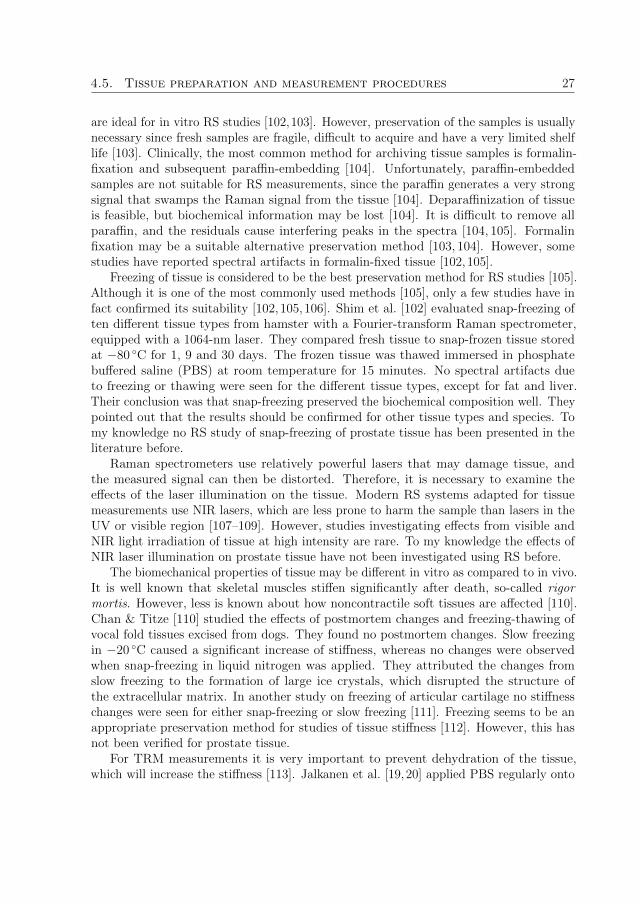
The diagnosis of PCa is determined through histological analysis of tissue sectionsfrom the biopsy samples or from the removed prostate when surgery has been performed.Montironi et al. [56] give a detailed description of a recommended procedure for preparationof radical prostatectomy specimens. In brief, first the removed prostate is fixed by injectionof formalin at multiple sites using a needle. The surface is inked, and the prostate isimmersed into formalin for 24 hours. The prostate is then cut into 4-mm thick slices,which are embedded in paraffin. A microtome is used to cut a 5-µm thick specimenfrom each of the embedded slices. The specimens are stained with hematoxylin andeosin to induce contrast for histological examination. Under a light microscope a trainedobserver can recognize different tissue types and distinguish healthy and cancerous tissue(Figure 4.2). The aggressiveness of detected tumors can be assessed from the histologicalappearance of the prostatic glands following the Gleason grading system [55]. This methodis subjective, and the rates of intra- and interobserver disagreement are high [55]. Theseverity of PCa is clinically rated using a standardized system that defines different stagesdue to Gleason score and the spread of the primary tumor and metastases [44]. Today thepatients diagnosed with PCa have tumors of lower grade and lower stage than 20 yearsago, but there is still a wide range of aggressiveness [7]. Most patients have tumors ofmedium Gleason score, and due to the deficiencies in the practice of the Gleason systempredictions of disease progression are often uncertain [55]. The physicians are then facedwith a weak foundation for choosing an appropriate treatment.
The main imaging methods for detection of PCa are transrectal ultrasound and MRI.Due to a number of limitations, these techniques are not yet routinely used clinically fordirect PCa detection [7, 57]. New advances are very promising, but further clinical trialsare needed [57,58].
4.2.5 Treatments of prostate cancer
Radical prostatectomy is the recommended treatment for men with aggressive, localized(no metastases present) PCa [15]. It has excellent long-term PCa-specific survival rates [59].Unfortunately, serious side effects are common. Coelho et al. [60] estimated that > 40%of the patients were impotent and about 20% were incontinent 12 months after surgery.Today a rapidly increasing amount of radical prostatectomy procedures are performedusing robotic assistance, which shows promise for improving surgical quality and decreasing

4.3. Tactile resonance method 15
Epithelium
Stroma
Lumen
CancerStones
Healthy
Figure 4.2: A scan (ScanScope CS, 20× objective, Aperio, Vista, CA, USA) of a histologyspecimen from the prostate of a 67-year old man who was diagnosed with PCa and underwentradical prostatectomy. The dimensions of the scanned area are 4 × 1 .4 mm. The black lineindicates the border between healthy and cancerous tissue.
side effects [60,61].After surgery the PSA level is monitored to assess the effectiveness of the treatment.
For approximately 35% of patients, PSA will be detectable within ten years after surgery,which indicates clinically significant cancer recurrence [62,63]. The risk is increased foraggressive cancers and if positive surgical margins are present [16]. Whether patients withaggressive, localized tumors who underwent radical prostatectomy would benefit fromadditional treatment using radiotherapy, chemotherapy, hormonal therapy or combinationsof these is controversial [15, 64]. About 50% of those patients are cured with surgeryalone, and they are then spared the side effects and toxicity of additional therapy [15].Interestingly, van der Kwast et al. [62] found that adjuvant radiotherapy was significantlybeneficial only for patients with positive surgical margins. The study included 1005 men.Thus, to reduce the rate of cancer recurrence while minimizing the use of unnecessaryadjuvant therapy a method for intraoperative analysis of the surgical margins is greatlyneeded.
4.3 Tactile resonance method
4.3.1 The piezoelectric effect
The piezoelectric effect was discovered by the brothers Pierre and Jacques Curie in1880 [65]. They demonstrated that when pressure was applied to a crystal, such asquartz or topaz, an electric potential was generated. The inverse effect also applies, apiezoelectric element changes shape if exposed to an electric field, and will thereforeoscillate in response to a sinusoidal voltage variation. A piezoelectric element works as atransducer between electric and kinetic energy. The phenomenon originates from the factthat the unit cells of a piezoelectric material behave like electric dipoles, i.e. a non-uniform

16 Introduction
charge distribution arises because the elementary cells have no center of symmetry. Ifpressure is exerted on the material the shape of the dipoles is altered, and this will inducea net electric potential in the material. Resonance sensors are typically made from aceramic piezoelectric material, e.g. lead zirconate titanate (PZT), which can be picturedas a mass of tiny crystals, so-called crystallites, exhibiting dipole characteristics. The unitcells of the crystallites are non-centrosymmetric below the Curie temperature (the criticalpoint below which the material is ferromagnetic), which usually is of the order of 1000 K(∼ 700 ◦C) [66]. A ceramic can be given its piezoelectric properties by heating it to justbelow the Curie temperature and applying a strong electric field over it. The ceramic isthen polarized in the direction of the applied field, and the dipoles are locked when thefield is withdrawn.
4.3.2 Principle of the tactile resonance method
The principle of the TRM was presented by Omata & Terunuma in 1992 [67]. It is basedon a piezoelectric PZT transducer divided into two parts, a driving element that generatesvibration, and a pick-up element that detects the frequency of vibration. The transducer isset into oscillation by an electronic feedback circuit consisting of an amplifier, a bandpassfilter and a phase-shift circuit, as shown in Figure 4.3 [67]. The signal from the pick-up isfed back to the circuit. The phase-frequency characteristics of the PZT transducer and theelectronic circuit determine the oscillation frequency of the whole system. The phase-shiftcircuit establishes resonance at a user-selected frequency by ensuring that the sum ofthe phase shifts in the system is zero. To obtain a high sensitivity it is advantageousto choose a frequency close to the inherent resonance frequency of the PZT element. Aprobe tip is glued to the end of the PZT element (Figure 4.3). It is made in a shapeand from a material suitable for the measurement task at hand. As the tip comes intocontact with an object the resonance frequency changes, and the shift is related to thestiffness of the material [67]. The absolute frequency shift increases with the stiffness ofthe probed material. For relatively soft objects, such as silicone gum and the palm ofa hand, the shift is negative, whereas it is positive for hard materials such as teeth andglass [67]. Murayama & Omata [68] developed an MTS by using a tip in the form of a30 mm long, tapered glass needle with a very small spherical tip, from 1 mm down to0.1 µm in diameter.
4.3.3 Theory
Kleesattel & Gladwell introduced a surface hardness tester called the contact-impedancemeter in two publications in 1968 [69, 70]. Their theoretical explanations could laterbe applied to describe the characteristics of the TRM [67, 71]. A piezoelectric tactileresonance sensor can be modeled as a finite rod vibrating at its resonance frequency inthe direction of its length [67, 69–71]. The probe tip is assumed to be hemispherical. Thefrequency change as the sensor comes in contact with an object can be expressed as
∆f = − V0βx2πlZ0
(4.1)

4.3. Tactile resonance method 17
Feedback circuit
Phase-shiftcircuit
Probe tip
elementDriving
PZT
Amplifier
Bandpassfilter
Pick-up
Figure 4.3: The principle of the TRM.
where V0 is the wave velocity in the rod, l is the length of the rod, Z0 is the acousticimpedance of the rod and βx is the reactance part of the acoustic impedance
Zx = αx + iβx (4.2)
of the probed object, where αx is the resistance. βx can be written as
βx = mxω −kxω
(4.3)
where ω is the angular frequency, mx is the contact mass and kx is the contact stiffness.mx and kx depend on the surface contact area S and can be written as
mx =4a11
π 3/2(1− ν)ρS 3/2 (4.4)
kx =2E
π 1/2(1− ν2) S1/2 (4.5)
ν is Poisson’s ratio, ρ is the density, E is the elastic modulus (Young’s modulus), and a11is a coefficient that depends on ν [70]. S = πr2, where r is the radius of the contact area.From (4.3)–(4.5) we see that for large contact areas mx will dominate, whereas kx willdominate for small contact areas [67]. Furthermore, at high frequencies the contributionfrom mxω increases, whereas kx/ω becomes more important at low frequencies.
Jalkanen et al. [71] examined the theoretical model of the finite rod for theVenustron®
system. The resonance frequency was 58 kHz and the probe had a hemispherically shaped

18 Introduction
tip with 5 mm diameter. They showed that, since mxω � kx/ω for that system, thesurface stiffness term kx/ω in (4.3) can be neglected. (4.1)–(4.4) then give
∆f ∝ ρS 3/2 (4.6)
for a specific rod vibrating at a constant frequency, if Poisson’s ratio is assumed to beconstant [71]. The surface contact area S depends on the contact force between thesensor tip and the measurement object, F , according to F ∝ ES 3/2 [71]. Substitutingthis relationship into (4.6) results in
∆f ∝ρF
E(4.7)
A stiffness sensitive parameter ∂F/∂∆f can then be derived as
∂F
∂∆f∝E
ρ(4.8)
Jalkanen et al. [71] experimentally verified this theoretical model in measurements onhuman prostate tissue. Their study showed that density variations were small and mostlynon-significant, validating the use of ∂F/∂∆f as a stiffness sensitive parameter.
For the MTS the contact area is small and the inertia term mxω will be smaller thanthe surface stiffness term kx/ω and can usually be neglected [72]. (4.1) can then bewritten as
∆f =V0kx
2πlZ0ω(4.9)
According to Murayama & Omata [68] Hertz theory can be applied for small indentationdepths δ, and the contact area S can then be modeled as a function of δ. They showedthat from (4.5) and (4.9) a stiffness sensitive parameter can be obtained as ∆f/δ, whichis related to Young’s modulus [68]. They calculated Young’s modulus from the slope ofthe frequency versus indentation curve, and verified that ∆f/δ correlated highly with Ein experiments on silicone samples.
4.3.4 Sensing volume
Jalkanen et al. [21] investigated the sensing volume of the Venustron® TRM system. Theyconcluded that the tip laterally sensed a larger area than the actual contact area andhad an estimated penetration depth of 3.5–5.5 mm for an indentation depth δ = 1 mm.There was an approximate linear relationship between the indentation depth and thesensing depth; the sensor probed deeper into the tissue at larger indentation depths. Forδ = 2 mm the penetration depth was estimated to be up to 10 mm. Using an array with64 TRM sensor elements Murayama et al. [73] demonstrated that tumors in the breastlarger than 10 mm could be detected at depths up to 20 mm. TRM has higher potentialfor noninvasive detection of PCa than RS.

4.4. Raman spectroscopy 19
4.3.5 Detection of prostate cancer
Eklund et al. [37] were the first group to measure the stiffness of human prostate tissueusing TRM in vitro. A catheter type sensor was used. The catheter was 2 mm in diameter.A hemispherical tip was formed from epoxy and attached to the PZT element, sealing theend of the catheter. They used a proposed model where the tissue stiffness was linearlyrelated to the amounts of glandular tissue and prostate stones. A correlation of R = −0.96between the measured and the expected stiffness was found. The tissue was fixed informalin, which in general hardens the tissue. The results indicated that stroma andprostate stones were relatively hard tissue components, while glandular tissue was softer.Jalkanen et al. [19,20] examined fresh human prostate tissue with the Venustron® system.A slice of prostate was measured directly after surgical removal. The authors showed thatTRM could distinguish glandular tissue from cancerous tissue. In the first study [20] tensamples from ten patients were tested. A p-value < 0.001 was obtained for a MANOVAtest of the difference between cancerous (n = 13) and healthy (n = 98) tissue. Onlymeasurement sites consisting of 100% cancerous tissue were significantly stiffer than theglandular tissue. Stroma and sites with an accumulation of prostate stones could not bedifferentiated from cancer in those studies. However, PCa usually develops in the posteriorpart of the prostate [45, 46], where glandular tissue is abundant [19]. Thus, a stiff nodulein this area could indicate cancer [19]. In a recent study [74] Jalkanen demonstrated thathand-held measurements using the Venustron® could accurately determine the stiffnessof gelatin (R2 = 0.94). For hand-held measurements the impression speed is unknown,but Jalkanen showed theoretically and experimentally that this factor is not significantlyrelated to the measured stiffness, which is promising for in vivo measurements. Murayamaet al. [75] used an elasticity mapping system with an MTS to scan 300 µm-thick prostatesections from two patients. The tip of the MTS was 10 µm in diameter, and the scanningstep-size was 5 µm. They found that the proportion of stiff points was larger for canceroustissue. However, the stiffness distribution of healthy and cancerous tissue overlapped. Nostatistic evalution was performed.
4.4 Raman spectroscopy
4.4.1 The Raman effect
When a laser beam illuminates a tissue sample most photons are elastically scattered,i.e. their energy is conserved. A fraction of the photons are inelastically scattered andloose or gain energy as they interact with the biological molecules. There are three maininelastic scattering events: fluorescence, phosphorescence and Raman. Fluorescence andphosphorescence are associated with electronic transitions of the participating molecules.Raman scattering is a relatively weak process (quantum yield 10−8–10−6) in which incidentphotons set molecular bonds into vibration [76]. The energy of the scattered photons isshifted corresponding to the difference between the initial and final vibrational energylevels. A Raman spectrum is a plot of the scattered intensity versus the energy shifts.

20 Introduction
Since every molecule has a unique set of bond vibrations, the spectrum is like a fingerprintof the sample. By convention the energy shift is expressed as a wavenumber shift termedStokes shift and measured in cm−1 (the number of wavelengths per cm) [77]:
∆ν =1
λi− 1
λe(4.10)
where λi and λe are the wavelengths of the incident and emitted photons, respectively.The Raman effect was predicted by quantum mechanics in publications by Smekal
in 1923 and Kramers & Heisenberg in 1925 [78]. It was experimentally verified in 1928by the Indian professor Sir C. V. Raman. He observed the phenomenon in a delicateexperiment using filtered sunlight as excitation source, a telescope to collect the scatteredlight and the eye as detector [79]. He was awarded the Nobel prize for the discoveryalready two years later.
Classical physics explains the basic principles of Raman scattering [76, 80]. As amolecule is hit by a photon its electron cloud is distorted by the electromagnetic field. Thegeometry of the cloud is changed and the molecule is excited to a virtual, higher state ofenergy. This state is unstable; the nuclei of the molecule cannot establish new equilibriumpositions in response to the rearrangement of electrons. As the molecule relaxes thenuclei are set into vibration and a photon is emitted. The process is fast (10−13–10−11 s)compared to fluorescence (10−9–10−7 s) [81]. Consider a diatomic molecule irradiated bymonochromatic light with frequency ν0. The electrical field E = E0 cos (2πν0t), where tdenotes time, induces a dipole moment
P = αE = αE0 cos (2πν0t) (4.11)
in the molecule. The polarizability α is a function of the nuclear displacement, becauseas the molecule changes shape, size or orientation the electron cloud can become easieror more difficult to distort. If the nuclei vibrate with a frequency νm, the nucleardisplacement q can be expressed as q = q0 cos (2πνmt), where q0 is the amplitude of theoscillation. Since α(q) can be regarded as a linear function of q for small amplitudes ofvibration, it can be expanded as
α = α0 +
(∂α
∂q
)0
q + . . . (4.12)
where α0 is the polarizability at q = 0. Substituting (4.12) into (4.11), and using theformula cos γ cos β = 1
2cos (γ − β) + 1
2cos (γ + β), we obtain
P = α0E0 cos (2πν0t)︸ ︷︷ ︸elastic
+1
2
(∂α
∂q
)0
q0E0
cos (2π(ν0 − νm)t)︸ ︷︷ ︸Stokes
+ cos (2π(ν0 + νm)t)︸ ︷︷ ︸anti-Stokes
(4.13)
The three terms in (4.13) symbolize dipoles that oscillate with frequencies ν0, ν0 − νmand ν0 + νm. They describe elastic, Stokes and anti-Stokes scattering, respectively. Inanti-Stokes scattering the photons gain energy. This is possible only when the molecule

4.4. Raman spectroscopy 21
ν0
ν1
ν2
ν3
ν4
Elastic
Vibrationalstates
Energy
Virtualstates
Stokes anti-Stokes
First electronicexcited state
Figure 4.4: Energy diagram of elastic and Raman scattering. Incident photons are shown asupward arrows and emitted photons as downward arrows.
initially is at a higher vibrational energy level (Figure 4.4). At room temperature higherlevels are sparsely populated and anti-Stokes scattering is weak. A fundamental property
of the Raman effect is understood from (4.13): if(∂α∂q
)0
= 0, no Raman scattering
will occur. This means that a specific molecular vibration is Raman active only if thepolarizability is changed during the vibrational cycle. Symmetric vibrations usually causethe largest polarizability changes and generate the strongest scattering [76]. In generalthe scattering intensity I depends on the laser power lp, the frequency of the laser light,ν0, and the polarizability α, according to [76]:
I ∝ lpα2ν40 (4.14)
Hence, the Raman intensity is much stronger if a laser with short wavelength is used.Quantum physics can be applied to calculate the frequencies of the molecular vibra-
tions [80]. As an example, consider the vibration of a diatomic molecule. It can bemodeled as a harmonic oscillator for a single particle. The chemical bonding betweenthe nuclei is pictured as a Hookian spring with a force constant k, and the potentialenergy V (q) = 1
2kq2, where q is the displacement. The Schrodinger equation for this
model becomes
− h2
8π2m
∂2Ψ
∂q2+
1
2kq2Ψ = EΨ (4.15)
h is Planck’s constant, m is the mass of the particle, Ψ is the wave function and E isthe total energy of the particle. The solutions are eigenfunctions with the corresponding

22 Introduction
eigenvalues
Eυ = hcν
(υ +
1
2
)(4.16)
c is the speed of light, υ = 0, 1, 2, . . . is the vibrational quantum number, and
ν =1
2πc
√k
m(4.17)
is the wavenumber [cm−1] of the vibration. Hence, the rule of thumb is that strongbonds and light atoms will give rise to high vibrational frequencies and vice versa [76].From (4.16) we see that the energy is quantized with a constant separation betweenenergy levels equal to hcν. This is a good approximation for lower energy levels, butfor actual molecules the separation decreases av ν increases [80]. The selection rulesof quantum mechanics prohibit many vibrational transitions [80]. For the harmonicoscillator, only transitions that fulfill ∆υ = ±1 are allowed. The transition υ = 0 ↔ 1normally produces the most intense peak in the Raman spectrum, since most moleculesare in their lowest state of energy E0 at room temperature. For polyatomic moleculesthe vibrational patterns can be very complicated. However, in principle the complicatedvibrations can be described as a superposition of harmonic oscillations for all nuclei [80].
4.4.2 Instrumentation
A Raman spectrometer basically consists of a laser generating monochromatic light, asample illumination and collection system, a filter that separates the elastically- and theinelastically-scattered light, a wavelength selector (e.g. a grating) and a detector [80].Modern systems for tissue measurements typically use NIR diode lasers and CCD detec-tors [82]. Microscopes or fiber optic probes in the backscattering collection geometry arecommonly used to illuminate the sample and collect the Raman light [30]. Figure 4.5shows a schematic drawing of an RS fiber optic setup.
The development of RS fiber optic probes enables in vivo measurements. Severalfactors complicate the realization of fiber optic probes. Fused silica fibers generate a strongsignal in the Fingerprint spectral interval, which necessitates the use of extra filters at theprobe tip to block this radiation [28]. For clinical use the probes need to be flexible andthin, of the order of 1–2 mm to be incorporated into biopsy needles, endoscopes and otherdevices [83]. They must withstand clinical sterilization routines [83]. Several differentprobes have been developed, but so far the manufacturing process has been complicatedand expensive [28]. However, several technical advancements in the construction of fiberoptic probes have been presented recently [28,84,85]. Furthermore, RS measurements inthe high wavenumber region, from 2400 to 3800 cm−1, can be performed using simplerprobes without filters, since little Raman signal is generated in the probe itself in thisregion [86–88].
Komachi et al. [89–92] have developed a 0.6 mm thin probe, and demonstratedpromising results in measurements of the esophagus and stomach of the living rat [92].The probe consists of a central delivery fiber surrounded by eight collection fibers. They

4.4. Raman spectroscopy 23
������������������
������������������Spectrometer
LaserFilter Grating CCD
Computer
Sample
Fiber optic probe
Figure 4.5: A typical RS fiber optic setup.
claim that it can be commercially manufactured at a low cost [89]. Day et al. [84] describethe development of a miniature, confocal fiber optic probe. Their aim was to constructa probe capable of sampling tissue layers 100–200 µm below the tissue surface, whichwould be optimal for early detection of esophageal cancer. The depth of field was 147 µmin measurements on polished silicon. In a recent publication the group attained 66–81%sensitivity and 80–98% specificity for discriminating esophageal cancer from healthy tissueusing that confocal probe with an integration time of 2 s [85]. They measured 123 biopsysamples from 49 patients. The accuracy was increased for an integration time of 10 s.
The penetration depth in tissue of RS fiber optic probes using the backscatteringcollection mode is typically only several hundred micrometers [30]. Hence, deep-sitedorgans, such as the prostate, are inaccessible for noninvasive examinations. Develop-ment of RS techniques that can probe deeper into the tissue, such as time-gated RS,transmission RS, and spatially offset probes, is ongoing [30]. Spatially offset probesincrease the accessible depth to several mm [30]. However, the spatial separation betweenexcitation fibers and collection fibers makes the probes bulkier than ordinary probes.Using transmission RS identification of calcified materials buried at depths up to 2.7 cm ina breast cancer phantom have been demonstrated [93]. However, in transmission RS thesample is illuminated from one side and the Raman signal is collected from the oppositeside; this approach may be difficult to use in vivo.
4.4.3 Raman measurements of tissue
RS is excellent for measuring the biochemical content of tissue for a number of reasonsincluding:
r The majority of biological molecules are Raman active [81].

24 Introduction
r Minimal or no sample preparation is required.
r Water is a poor Raman scatterer; it interferes little with the spectra of tissue [76].
r RS is sensitive to many factors that affect biomolecules, such as pH, degree ofhydration, bacterial attack, etc. [94].
r The relative abundance of tissue components is proportional to their contributionsto the Raman spectrum [83].
r In vivo measurements are feasible via fiber optic probes.
Some of the drawbacks with the method are:
r Tissue autofluorescence can distort the Raman signal.
r Acquisition of high quality spectra often requires long integration times. Therefore,in vivo measurements may be affected by motion artifacts.
r The instrumentation is sensitive to surrounding light.
r Current fiber optic probes have a short penetration depth in tissue [30].
RS measurements of tissue were long hampered by the strong, broadband tissue autofluo-rescence induced by lasers in the visible region [83]. Modern NIR RS systems have largelyovercome this problem, since NIR light has too low energy to initiate most fluorescenceprocesses [83]. Autofluorescence of tissue is believed to be generated mainly by a fewfluorophores such as flavins, nicotinamide adenine dinucleotide, aromatic acids such astryptophan, tyrosine and phenylalanine, and porphyrins [95]. Several different approachesfor minimizing fluorescence interference have been demonstrated. Time-gating and wave-length shifting can effectively decrease fluorescence, but these require modifications of theRaman instrumentation [96]. An alternative is to use mathematical methods to subtractthe fluorescence signal. However, many algorithms cause spectral artifacts [96]. Polynomialfitting does not distort the Raman peaks to a high degree [96]. Lieber et al. [96] presentedan algorithm that automatically subtracts the spectral background by fitting a modifiedpolynomial to the spectrum. This method was further developed by Cao et al. [97].
The origin of many observed peaks in tissue spectra can often be interpreted with help ofdatabases and published spectra of biological molecules [81,98]. Tissue generally producesspectra with relatively narrow bands, typically 10–20 cm−1 wide [83]. Stokes shifts from200–3600 cm−1 usually cover the information of interest [76]. The characteristic vibrationsof the most common chemical groups have been assigned approximate wavenumber rangesthat are valid for the groups in most structures [76]. The spectral region 4000–2500 cm−1
is where single bonds (X−H) scatter, the interval 2500–2000 cm−1 is where multiplebonds (−N=C=O) occur, and the range 2000–1500 cm−1 includes double bonds (−C=O,−C=N, −C=C−). The interval 1900–700 cm−1 is referred to as the Fingerprint region.Many molecules exhibit complex vibrational patterns that yield unique spectral featuresin this region, which is densely packed with sharp bands [81]. Raman peaks below

4.4. Raman spectroscopy 25
534
621
760
816
856
877
939
1004
1032
1208
1245
1451
1666
intensity
(arb)
Raman shift (cm−1)
400 600 800 1000 1200 1400 1600 1800
Figure 4.6: A spectrum of porcine prostate tissue recorded in our laboratory using a Raman microspectrometer (Renishaw system 2000, Renishaw, Wotton-under-Edge, UK). The integration timewas five minutes.
650 cm−1 normally belong to inorganic groups, metal-organic groups or lattice vibrations.RS can explore the primary, secondary, tertiary and quaternary structure of biologicalmolecules [81]. For example protein structure, DNA conformation and cell membraneconformation can be probed. Databases over characteristic peak frequencies of importantbiological molecules are available, see e.g. Movasaghi et al. [98]. Figure 4.6 shows anexample of a porcine prostate spectrum. Tentative assignments of the major peaksidentified in the spectrum are given in Table 4.1.
There is an abundance of diagnostic features for cancer detection in the spectra ofvarious tissues [81]. The ratio of intensities of the amide I vibrational mode at 1655 cm−1
to the CH2 bending vibrational mode at 1450 cm−1 can be used to differentiate healthy andcancerous tissue in brain, breast and gynecological tissues. Cancer induces a significantincrease of the DNA content [27,81,99]. The amide III band at 1260 cm−1 may contributetowards cancer identification, e.g. the amide III band is broadened in cancerous gynecologictissue.
Several in vitro studies [24–27, 29, 99, 101] have investigated the potential of RS todetect and grade PCa. Crow et al. [25] attained 98% sensitivity and 99% specificity fordifferentiating four cell lines with varying degrees of aggressiveness. Cells were placedonto a calcium fluoride slide, and about 50 spectra from each cell line were measured.A total of 200 spectra were input to the diagnostic algorithm, which used principalcomponent analysis (PCA) and linear discriminant analysis. Taleb et al. [99] attained a100% accurate classification of healthy and cancerous (derived from metastases) prostatecells (n = 30). They concluded that the most significant spectral change due to cancer

26 Introduction
Table 4.1: Tentative assignments [98–100] of the major peaks in the porcine prostate spectrumshown in Figure 4.6.
Peak position (cm−1) Assignments
1666 Amide I (proteins)/C=C lipid stretch1451 CH2 bending mode of proteins and lipids1245 Amide III (proteins, 1240–1265 cm−1)1208 Tryptophan and phenylalanine ν(C−C6H5) mode1032 C−H in-plane bending mode of phenylalanine1004 Symmetric ring breathing mode of phenylalanine939 C−C stretching of collagen backbone877 C−C stretching (collagen)/C−C−N+ stretching (lipids)856 Ring breathing mode of tyrosine/C−C stretch of proline ring816 C−C stretching (collagen)/proline, tyrosine, ν2 PO−2 stretch
of nucleic acids760 Symmetric breathing of tryptophan621 C−C twisting mode of phenylalanine534 S−S disulfide stretch in proteins
was an increase in the DNA content and a change in DNA conformation from B-DNAto A-DNA. Crow et al. [24] showed that prostate biopsy samples of BPH and cancerwith different Gleason scores could be distinguished with an overall accuracy of 89%.They recorded 450 spectra from biopsies of 27 patients, 14 with BPH and 13 with PCa.Devpura et al. [29] identified > 94% of cancerous regions in RS measurements on 10 µmthick prostate specimens. They found that Gleason scores 6, 7 and 8 could be clearlyseparated. In the only publication using a fiber optic probe [26], PCa was distinguishedfrom BPH and prostatitis with an overall accuracy of 86%. 38 prostate samples from37 patients were measured. Stone et al. [27] estimated the gross biochemistry of BPH,prostatitis and PCa of different grades of aggressiveness (Gleason score < 7, = 7 and > 7).This was accomplished by comparing the spectra of the prostate samples to the spectraof pure chemical standards assumed to be the main tissue components. It was shownthat the DNA content was increased in cancerous tissue. Furthermore, the cholesterollevel increased substantially, the choline level was elevated but remained low, triolein wasincreased, while oleic acid decreased somewhat with progression of disease.
4.5 Tissue preparation and measurement procedures
In vitro experiments should be carefully designed so that the results and conclusions thereofare applicable to in vivo measurements. It is essential to avoid misinterpretation of resultsdue to artifacts originating from tissue preparation and/or inappropriate measurementprocedures.
Fresh tissue samples, immersed in physiological buffer to prevent tissue dehydration,
4.5. Tissue preparation and measurement procedures 27
are ideal for in vitro RS studies [102,103]. However, preservation of the samples is usuallynecessary since fresh samples are fragile, difficult to acquire and have a very limited shelflife [103]. Clinically, the most common method for archiving tissue samples is formalin-fixation and subsequent paraffin-embedding [104]. Unfortunately, paraffin-embeddedsamples are not suitable for RS measurements, since the paraffin generates a very strongsignal that swamps the Raman signal from the tissue [104]. Deparaffinization of tissueis feasible, but biochemical information may be lost [104]. It is difficult to remove allparaffin, and the residuals cause interfering peaks in the spectra [104, 105]. Formalinfixation may be a suitable alternative preservation method [103, 104]. However, somestudies have reported spectral artifacts in formalin-fixed tissue [102,105].
Freezing of tissue is considered to be the best preservation method for RS studies [105].Although it is one of the most commonly used methods [105], only a few studies have infact confirmed its suitability [102,105,106]. Shim et al. [102] evaluated snap-freezing often different tissue types from hamster with a Fourier-transform Raman spectrometer,equipped with a 1064-nm laser. They compared fresh tissue to snap-frozen tissue storedat −80 ◦C for 1, 9 and 30 days. The frozen tissue was thawed immersed in phosphatebuffered saline (PBS) at room temperature for 15 minutes. No spectral artifacts dueto freezing or thawing were seen for the different tissue types, except for fat and liver.Their conclusion was that snap-freezing preserved the biochemical composition well. Theypointed out that the results should be confirmed for other tissue types and species. Tomy knowledge no RS study of snap-freezing of prostate tissue has been presented in theliterature before.
Raman spectrometers use relatively powerful lasers that may damage tissue, andthe measured signal can then be distorted. Therefore, it is necessary to examine theeffects of the laser illumination on the tissue. Modern RS systems adapted for tissuemeasurements use NIR lasers, which are less prone to harm the sample than lasers in theUV or visible region [107–109]. However, studies investigating effects from visible andNIR light irradiation of tissue at high intensity are rare. To my knowledge the effects ofNIR laser illumination on prostate tissue have not been investigated using RS before.
The biomechanical properties of tissue may be different in vitro as compared to in vivo.It is well known that skeletal muscles stiffen significantly after death, so-called rigormortis. However, less is known about how noncontractile soft tissues are affected [110].Chan & Titze [110] studied the effects of postmortem changes and freezing-thawing ofvocal fold tissues excised from dogs. They found no postmortem changes. Slow freezingin −20 ◦C caused a significant increase of stiffness, whereas no changes were observedwhen snap-freezing in liquid nitrogen was applied. They attributed the changes fromslow freezing to the formation of large ice crystals, which disrupted the structure ofthe extracellular matrix. In another study on freezing of articular cartilage no stiffnesschanges were seen for either snap-freezing or slow freezing [111]. Freezing seems to be anappropriate preservation method for studies of tissue stiffness [112]. However, this hasnot been verified for prostate tissue.
For TRM measurements it is very important to prevent dehydration of the tissue,which will increase the stiffness [113]. Jalkanen et al. [19, 20] applied PBS regularly onto
28 Introduction
the prostate slices during measurements using a brush. Murayama, Oie et al. [75, 114]used a moisture chamber at 36 ◦C for elasticity mapping with the MTS. The group laterrefined the experimental setup to let the tissue sample and the MTS be fully immersedin PBS [113,115], which enabled measurements to be acquired for several hours withoutartifacts [115].
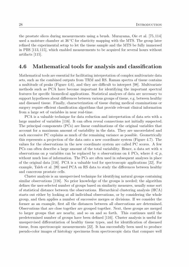
4.6 Mathematical tools for analysis and classification
Mathematical tools are essential for facilitating interpretation of complex multivariate datasets, such as the combined outputs from TRM and RS. Raman spectra of tissue containsa multitude of peaks (Figure 4.6), and they are difficult to interpret [98]. Multivariatemethods such as PCA have become important for identifying the important spectralfeatures for specific biomedical applications. Statistical analyses of data are necessary tosupport hypotheses about differences between various groups of tissue, e.g. between healthyand diseased tissue. Finally, characterization of tissue during medical examinations orsurgery require efficient classification algorithms that provide relevant clinical informationfrom a large set of variables in near real-time.
PCA is a valuable technique for data reduction and interpretation of data sets with alarge number of variables [116]. It can often reveal connections not initially suspected.The principal components (PCs) are linear combinations of the original variables thataccount for a maximum amount of variability in the data. They are uncorrelated andeach successive PC explains as much of the remaining variance as possible. Geometricallythis represents a projection of the data onto a new coordinate system (Figure 4.7). Thevalues for the observations in the new coordinate system are called PC scores. A fewPCs can often describe a large amount of the total variability. Hence, a data set with nobservations on p variables can be replaced by n observations on k PCs, where k � p,without much loss of information. The PCs are often used in subsequent analyses in placeof the original data [116]. PCA is a valuable tool for spectroscopic applications [22]. Forexample, Taleb et al. [99] used PCA on RS data to study the differences between healthyand cancerous prostate cells.
Cluster analysis is an unsupervised technique for identifying natural groups containingsimilar observations [116]. No prior knowledge of the groups is needed; the algorithmdefines the user-selected number of groups based on similarity measures, usually some sortof statistical distance between the observations. Hierarchical clustering analysis (HCA)starts out either by looking at all individual observations, or by considering the wholegroup, and then applies a number of successive merges or divisions. If we consider theformer as an example, first all the distances between all observations are determined.Observations that are close together are grouped together. Next, these groups are mergedto larger groups that are nearby, and so on and so forth. This continues until thepredetermined number of groups have been defined [116]. Cluster analysis is useful forunsupervised differentiation of healthy tissue types, and for identification of diseasedtissue, from spectroscopic measurements [22]. It has successfully been used to producepseudo-color images of histology specimens from spectroscopic data that compare well

4.6. Mathematical tools for analysis and classification 29
X2
X1
PC 1
PC 2
Figure 4.7: PCA on random data from a bivariate normal distribution. The PCs are vectors ofunit length that point in directions of maximum variability. They will be the axes of the newcoordinate system. For this example the first PC explains almost 95% of the total variability.
with standard histology images [22,117].The objective of data classification is to define a rule that can decide to which class a
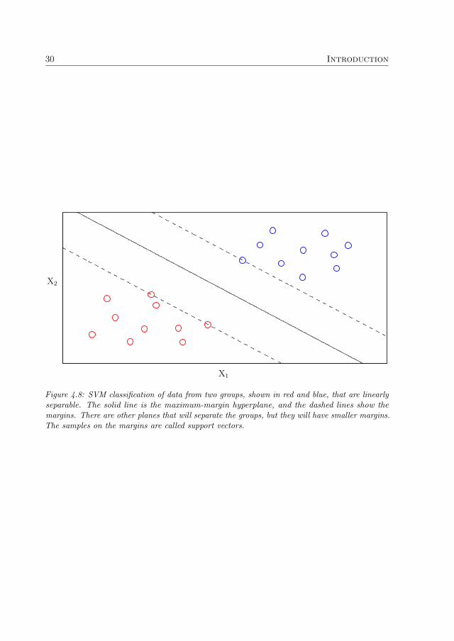
new observation belongs [116]. The rule is found by training the classifier to recognizepatterns in data from observations of a relatively large number of samples of knownclasses. Classification techniques are supervised, in contrast to cluster analysis, whereno classes are defined prior to analysis. Support vector machines (SVM) is a powerfulclassification technique that was introduced by Cortes & Vapnik in 1995 [118]. SVMcalculates the hyperplane that separates two classes of data with the largest possiblemargin (Figure 4.8). Cortes & Vapnik introduced the concept of soft margins that enablesclassification of nonseparable data. The algorithm aims at minimizing the number ofclassification errors while separating the correctly classified observations with maximalmargin [118]. To construct classification rules that generalize well, i.e. classify unseen datawith low rate of error [118], cross-validation techniques can be used to find the optimalparameter settings for the SVM algorithm [119]. SVM can be used to separate more thantwo classes [120]. One strategy is to apply the binary classifier to distinguish two classesat a time, and determine the final class from the outcomes for all those classificationsby a voting procedure [120]. SVM has attained very high classification accuracies inspectroscopic studies of cancerous tissues [121–123].
30 Introduction
X2
X1
Figure 4.8: SVM classification of data from two groups, shown in red and blue, that are linearlyseparable. The solid line is the maximum-margin hyperplane, and the dashed lines show themargins. There are other planes that will separate the groups, but they will have smaller margins.The samples on the margins are called support vectors.

Chapter 5
Aims
The overall aim of this thesis was to explore the need for new, complementary methodsfor PCa detection and take the first step towards a novel approach: the combination ofTRM and RS. The specific aims were:
r To review the different methods for localization and diagnosis of PCa, in order toexplore the demand for new, complementary methods.
◦ This objective was assessed in Paper A.
r To develop a robust procedure for RS measurements of tissue in vitro, and formathematical preprocessing and multivariate analysis of RS data. In particular, toevaluate the effects of snap-freezing and NIR laser illumination on porcine prostatetissue using RS.
◦ This objective was assessed in Papers B, C and D.
r To develop a multivariate approach for comparing TRM and RS information viameasurements on porcine tissue in vitro, in order to investigate the correlation ofthe data and potential diagnostic power of the combination.
◦ This objective was assessed in Paper C.
r To develop a novel setup combining a scanning haptic microscope employing anMTS and an RS fiber optic probe, and adapt the system for measurements ofprostate tissue slices.
◦ This objective was assessed in Paper D.
r To investigate the accuracy for classification of healthy porcine prostate tissuetypes, and healthy and cancerous human prostate tissue, using SVM classificationof combined TRM and RS measurements with the above-mentioned system.
◦ This objective was assessed in Paper D.
31

32 Aims

Chapter 6
Material and Methods
This chapter summarizes the practical part of the work. It describes the equipment that wasused, the measurement procedures and the data analysis. For more detailed informationthe reader is referred to Papers A–D.
6.1 Literature review
A review of the methods for localization and diagnosis of PCa was performed (A).The review focused on technical methods that can, or have the potential to, directlylocalize/diagnose PCa in situ via noninvasive or minimally invasive routes. Methodsthat label the tumor, e.g. with radioactive or fluorescent markers, were excluded. Thedatabases Science Citation Index Expanded® and Social Sciences Citation Index® weresearched via Web of Science®1 for relevant papers using the following combinations ofsearch words:
r prostate and cancer and imaging
r ultrasound and prostate
r prostate and spectroscopy not magnetic
r magnetic and resonance and prostate and cancer
r Raman and prostate
r resonance and sensor and prostate
r infrared and spectroscopy and prostate and cancer
r prostate and FTIR
r elastography and prostate
r DWI and prostate
r DCE MRI and prostate
1http://www.isiwebofknowledge.com
33
34 Material and Methods
All years of publication, 1975–2009, were included in the searches. Recent publicationswere favored. The reference lists in the selected articles were scrutinized for additionalimportant papers. 185 publications were eventually selected for the review.
6.2 Experimental setup
Back in 2006 the research subject of Biomedical Engineering had just been established atthe university. We did not have our own laboratory at that time. Therefore, a Ramanmicro spectrometer (Renishaw system 2000, Renishaw, Wotton-under-Edge, UK), whichwas available at the Dept. of Chemical Engineering and Geosciences, was adapted formeasurements of tissue. This was done by installing a NIR laser with 830-nm wavelength(Renishaw HPNIR, 300 mW) and changing the filters of the setup. This system wasused to study the effects of snap-freezing and NIR laser illumination on porcine prostatetissue (B). A water-dip objective (NIR Apo 60×/1.0W, Nikon, Tokyo, Japan) was used forspectral acquisition in the Fingerprint region, from 400 to 1800 cm−1. The irradiance ontothe samples was ∼ 3 · 1010 W m−2. To avoid interference from surrounding light the roomwas darkened during measurements. The spectrometer was calibrated for wavelength shiftdaily using the sharp silicon peak at 520 cm−1 as reference. The wavelength-dependentsensitivity of the CCD detector was calibrated using a tungsten halogen light source(LS-1-CAL, Ocean Optics, Dunedin, FL, USA).
A sophisticated laboratory for biomedical research was built up during 2006–2009. Astate–of–the–art RS fiber optic system was purchased. It was composed of a 0.8 mm thinfiber optic probe (Machida Endoscope Co., Tokyo, Japan), of the same type used in [92],connected to a Raman spectroscope (RXN1, Kaiser Optical Systems, Ann Arbor, MI,USA). The spectroscope had a holographic grating that enabled simultaneous collectionof the complete spectral interval from 100 to 3425 cm−1. It incorporated a 400-mWlaser at 785 nm (Invictus�, Kaiser Optical Systems). Proprietary software (iC Raman�,Kaiser Optical Systems) controlled the spectrometer. This setup was used for the RSmeasurements in Papers C and D. All RS measurements were performed in darkness,because spectral distortions from surrounding light were observed. The laser power waslimited to avoid damage of the fiber optic probe due to heat building up at the tip. InPaper C it was set to 160 mW corresponding to approximately 80 mW onto the sample.For Paper D the probe was replaced with a more heat-resistant one, allowing use of higherpower. The laser power was then set to 270 mW. This corresponded to an output effectat the probe tip of 140–150 mW. The integration time could be lowered from 30 s (C) to7 s (D) without sacrificing spectral quality. The system was calibrated for wavelengthshift and energy sensitivity once a month (HoloLab Calibration Accessory, Kaiser OpticalSystems).
For performing the first combined TRM and RS measurements (C) the Venustron®
(Axiom Co., Ltd., Koriyama, Fukushima, Japan) TRM system was used in combinationwith the RS fiber optic setup. A customized setup was constructed (Figure 6.1). TheRS fiber optic probe and the Venustron® sensor were mounted next to each other. Athree-dimensional translation stage assured that measurements were performed at the

6.2. Experimental setup 35
Venustron®
Translation stage
Styrofoam plate
Pork belly sampleFiber optic probe
Thermometer
Figure 6.1: The experimental setup for Paper C.
same points with both probes. It was composed of three one-dimensional stages (NRT100,Thorlabs, Newton, NJ, USA) with a common control unit (BSC103, Thorlabs). Todamp vibrations the whole setup was mounted on an optical table (PBG52513 – MetricUltraLight Series II breadboards, Thorlabs). The translation stage was controlled viaa labview� (version 7.0, National Instruments, Austin, TX, USA) program writtenin-house. A camera (Powershot S3 IS with close-up lens 500D and LAH-DC20 conversionlens adapter, Canon, Tokyo, Japan) was mounted above the setup. It was used to capturea picture of the tissue sample, which was loaded into the program. The user selected themeasurement points from the picture. The coordinate system defined in the programwas calibrated to have the origin at the top left corner of the picture. It was importantto assure that the sensors measured on the same points of the sample. Their positionswere calibrated by visually controlling that each sensor was positioned exactly above areference mark when the translation stage was moved to the corresponding coordinates.
For Paper D a novel TRM technology was used, the MTS, which was developed byMurayama & Omata [68, 124, 125]. Their research group has developed an elasticitymapping system using the MTS, which has been termed scanning haptic microscopy(SHM) [115]. It has been commercialized, and we purchased such a prototype (P&MCo., Ltd., Aizuwakamatsu, Fukushima, Japan). A unique setup that combined the SHMsystem with the RS fiber optic setup was developed (Figure 6.2). It was composed ofan XYZ-stage with a resolution of 0.01 µm and an actuator mounted on the Z-axis to

36 Material and Methods
manipulate the MTS. The system incorporated a camera (LifeCam Cinema�, Microsoft,Redmond, WA, USA) and a USB microscope (Dino-Lite AM413TL, AnMo ElectronicsCorp., Hsinchu, Taiwan), to capture film and photos of the sample and probes. Thetemperature was logged by resistance measurement of a platinum resistance element(FK1020 PT1000, Heraeus, Kleinostheim, Germany) with a multimeter (Fluke 45, FlukeCorp., Everett, WA, USA), connected to the computer via GPIB. A labview� programthat controlled the hardware was developed. It automated the measurements as far aspossible and collected all data except the RS data, which was recorded by the spectrometersoftware on a separate computer. The spectral acquisition could not be automaticallytriggered. Therefore, a photo diode was mounted close to the RS probe (Figure 6.2)to monitor when the laser was illuminating the sample. The shutter to the laser wasclosed by the spectrometer between the measurements. The spectrometer was set tocontinuous spectral acquisition, and the translation stage was moved to the next point asthe photo diode voltage decreased abruptly. The voltage was measured with a secondmultimeter (Agilent 34401A, Agilent Technologies, Inc., Santa Clara, CA, USA) via theGPIB interface.
The SHM system was adapted for measurements of prostate tissue (D). The standardsettings had to be adjusted and optimizations of the software were done. Since theprostate tissue was rather sticky the MTS was raised relatively far above the tissue aftereach measurement, approximately 100 µm, so that it detached from the tissue. Theimpression depth was set to about 40 µm, which made the mappings more stable forsamples with uneven surfaces, as compared to the standard setting of ≈ 25 µm (half ofthe tip diameter). Each MTS had unique characteristics (Figure 6.3). The length andexact shape of the glass needle is very important for obtaining high sensitivity [125]. Somesensors were not suitable for prostate tissue measurements. One reason was that thestiffness range of the prostate tissue was wide, from 2 to 200 kHz, and some sensors did notgive a linear response throughout this range. Another reason was that for some sensorsthe resonance frequency could change abruptly when very stiff points were measured. Itwas often challenging to identify a frequency where the sensitivity was high, the responselinear, and the measurements were stable. The needles were fragile and easily brokendue to operator mistakes. Several safety routines were implemented in the labview�program to avoid this.
The positions of the MTS and the RS probe relative to the stage were determinedby using a printed grid with 50 µm line thickness (D). A line intersection was used asreference mark. The MTS was aligned with the reference mark using the USB microscope.Since the RS probe was relatively large it was difficult to calibrate its position visually.Therefore, an RS mapping was performed. A cluster analysis was performed on thedata using an HCA algorithm. The mesurement points were divided into three groups,and a mapping image was constructed. The line intersection was then clearly visualized(Figure 6.4), and the position of the RS probe was determined with high accuracy.
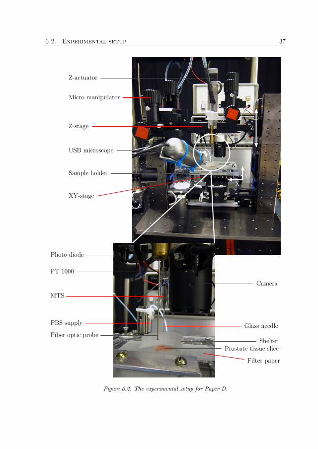
6.2. Experimental setup 37
USB microscope
Glass needle
Prostate tissue slice
Sample holder
Z-actuator
XY-stage
Z-stage
Shelter
Filter paper
Photo diode
PBS supply
Fiber optic probe
MTS
PT 1000
Camera
Y
X
Z
Micro manipulator
Figure 6.2: The experimental setup for Paper D.

38 Material and Methodsphase(degrees)
frequency (kHz)
gain
frequency (kHz)
50 100 150 200 250 300
50 100 150 200 250 300
0
200
400
600
0
50
100
150
200
250
Figure 6.3: The gain- and phase characteristics for one of the sensors used in Paper D. Thegain and phase for the selected frequency at 199.2 kHz are shown by the dashed lines. Usually ahigh sensitivity was obtained only in a narrow interval of a few kHz around a unique frequency.The best performance was often attained close to the second major peak in the gain-frequencycurve (top), which usually was present at around 200 kHz.
6.3 Sample preparation
For the study of the effects of laser illumination and snap-freezing (B) two porcineprostates were removed from boars slaughtered at the local abattoir. The prostates wereenclosed in a plastic bag and refrigerated. The prostates were not removed from theurethra and the surrounding, protective tissue until cut into smaller samples, which wasdone within 24 hours after slaughter. Samples were either stored in PBS in the refrigerator(referred to as fresh samples), or snap-frozen in liquid nitrogen and stored at −80 ◦C. Thefrozen samples were allowed to passively thaw immersed in PBS prior to measurement.
In Paper C pork belly tissue was used as a model system. Two pieces were obtainedfrom the local grocery store. They were stored at 6 ◦C. Two samples were cut from eachpiece, for a total of four samples. The samples were placed on a Styrofoam plate, whichwas fastened to the translation stage, as shown in Figure 6.1.
In Paper D both porcine and human prostate tissue were investigated. Eight porcine

6.4. Measurement procedure 39
y-coordinate(µm)
x-coordinate (µm)
0 100 200 300 4000
100
200
300
400
Figure 6.4: An example of a cluster analysis of RS data from a mapping over the line intersectionused as reference mark for spatial calibration.
prostates were collected from slaughtered boars. They were cut into smaller pieces, whichwere snap-frozen and cut into 500-µm thick slices using a freezing microtome. Adjacent toboth sides of each slice 5-µm thin specimens were cut. They were stained for histologicalanalysis. Small samples retrieved from the prostate of a patient undergoing radicalprostatectomy were snap-frozen in liquid nitrogen within thirty minutes after surgery.They were prepared in the same way as the porcine samples. Three of the samplescontained cancerous tissue and were included in the study. All samples were stored at−80 ◦C until measured.
6.4 Measurement procedure
To study the effects of laser illumination, repeated Raman spectra were acquired fromthe same point on the fresh tissue samples (B). The integration time was set to 10 s tocapture rapidly occurring effects. Spectra were captured subsequently during the firstminute, then less frequently during the following four minutes. For the snap-freezingexperiments five samples were measured day 1 and used as reference for fresh samples (B).Five snap-frozen samples were measured after 5, 26 and 81 days of storage, to study ifprolonged storage at −80 ◦C degraded the tissue. The samples were immersed in PBSduring the measurements.
For the combined TRM and RS measurements on pork belly tissue, a grid with 42measurement points was defined for each sample (C). In total 168 points were measuredwith each device. The measurement order was randomized with the constriction that

40 Material and Methods
adjacent points were not measured subsequently. This avoided the possibility thatviscoelastic effects would influence the TRM measurements. All TRM measurements ona sample were completed before the acquisition of Raman spectra. The tissue was keptmoist by brushing it with PBS every fifth minute. The distance from the RS probe tothe sample had to be adjusted manually. A magnifying glass was used to facilitate theadjustment.
For the combined measurements on porcine and human prostate tissue (D) dehydrationwas prevented by putting the samples on a filter paper soaked with PBS, which was puton top of a microscope slide with low spectral background (Calcium Fluoride UV grade,Crystran Ltd., Poole, UK). A shelter made from a rolled-up piece of a Kimwipe paper(Kimtech Science Kimwipes, Kimberly-Clark Inc., Roswell, GA, USA) was put aroundthe sample, and a constant flow of PBS was applied to it (Figure 6.2). The user set themeasurement region of interest in the labview� program. The MTS was set to thestarting position and the surface was detected through the frequency shift. A stiffnessmap and a topography map were then acquired with the MTS. The step size was 50 µm.Next the RS probe was moved to the starting position and a Raman map was capturedusing a 300 µm step size. The distance from the RS probe to the sample was adjusted tobe constant at 400 µm by using the topography map recorded by SHM.
6.5 Data analysis and statistics
All data analysis was performed using matlab® (version R2007b/R2008b/R2010a in-cluding Statistics Toolbox version 6.1/7.0/7.3, MathWorks Inc., Natick, MA, USA). Theonly exception was that minitab® (version 15.1.20.0, Minitab Inc., State College, PA,USA) was used to check for autocorrelation in Paper B. The algorithms not included inmatlab® were written in-house.
The RS data was preprocessed as follows (B–D). The Fingerprint region from 400–1800 cm−1 was selected. Wavelengths < 600 cm−1 were excluded due to interfering Ramanscattering generated in the fiber optic probe (C, D) [92]. Spectral spikes due to cosmic rayswere removed prior to analysis. Correction for the energy sensitivity of the spectrometerswas applied. Each Raman spectrum was lightly filtered using the smoothing algorithmby Eilers [126]. The background was automatically subtracted via the algorithm byCao et al. [97]. To aid comparison the spectra were vector normalized, so that theirintegrated areas were equal. In Paper D the variance minimization method [127] wasused to remove the Raman signal generated in the fiber optic probe and the interferingsignal from the filter paper. The Raman spectra were interpreted by making tentativeassignments of the peaks. The database collected by Movasaghi et al. [98] was frequentlyused. PCA was applied to the preprocessed Raman spectra to reduce the dimensionalityof the data (B, C). It was performed on unstandardized data, i.e. the variables were notscaled by dividing them by their standard deviations. The ten first PCs were retained forfurther evaluation. They explained a large percentage of the total variance.
In Paper B a modified version of Kim’s test [128, 129] was used to determine if themultivariate means of the PC scores of fresh and snap-frozen tissue differed. Three

6.5. Data analysis and statistics 41
analogous analyses were conducted, fresh tissue was compared to snap-frozen tissue storedat −80 ◦C for 5, 26 and 81 days. If the test showed a significant difference, Yuen’sunivariate test [130] was applied to compare the means of the individual PC scores. Thiswas done to investigate which PCs that contributed strongly to the significant multivariatedifference. The spectra of these PCs showed the main spectral differences between freshand snap-frozen tissue.
In Paper C the Raman PC scores were input to an unsupervised HCA algorithm usingWard’s linkage [116, 117]. The data set included all 168 spectra. The cluster analysisdivided the spectra into five groups. They were labeled A, B, C, D and E in Paper C, andwill here be represented by different colors: black, green, gray, red and blue, respectively.The TRM stiffness-sensitive parameter ∂F/∂∆f was calculated from ∆f , F and d as [19]
∂F
∂∆f=
∂F/∂d
∂∆f/∂d(6.1)
and evaluated at d = 0.6± 0.1 mm using linear regression (C). At this depth the sensormeasures the tissue near the surface [19]. The nonparametric Kruskal-Wallis test followedby Tukey-Kramer’s multiple comparison test were used to test if the mean stiffness ofthe groups differed. To evaluate the relationship between the TRM and RS informationa linear regression analysis was conducted using the Raman PC scores to explain thestiffness variation. Furthermore, receiver operating characteristic curves were constructedto investigate the ability of TRM to classify each tissue type defined by the cluster analysisof RS data. They showed the sensitivity and specificity for distinguishing the currenttissue type from the others for varying stiffness threshold values.
In Paper D three main tissue types were identified in the histologic analysis of theporcine samples: epithelium, lumen and stroma. For the human samples the groupswere: epithelium, lumen, stroma, cancerous epithelium, cancerous stroma and prostatestones. The stiffness sensitive parameter for the MTS, ∆f/δ, was calculated in matlab®.Furthermore, a measure of nonlinear effects was calculated by fitting a second-degreepolynomial to the frequency versus indentation curve for each measurement. Differencesin the biochemical composition of the tissue types were assessed by analyzing the meanspectra of the tissue types. The Kruskal-Wallis and Tukey-Kramer tests were used totest for significant differences in stiffness. An SVM analysis was performed to find theaccuracy of using the TRM alone, and TRM and RS together, to classify the tissue types.Different degrees of tissue homogeneity were analyzed (D).
A p-value less than 0.05 was considered as statistically significant for all statisticaltests. It was assumed that the experimental designs were completely randomized andthat the observations were independent.

42 Material and Methods
Chapter 7
General Results and Discussion
This chapter summarizes and explains the findings in Papers A–D, and discusses theirrelevance for the development of an instrument combining TRM and RS for PCa detection.
7.1 Literature review
The gold standard for PCa detection and diagnosis, the PSA test and SB, lacks sensitivityand specificity (A). Indolent and aggressive tumors cannot be reliably differentiated, andthe rate of overtreatment is high (A).
Grey-scale transrectal ultrasound is used only to guide biopsies to predetermined sitesaccording to SB protocols, since tumors usually cannot be discerned on the ultrasoundimage. Ultrasound techniques that assess the prostatic blood flow or tissue elasticity aremore effective (A). The best results have been obtained with contrast-enhanced ultrasound.Directing biopsies at suspicious lesions detects more clinically significant tumors withfewer biopsy cores, as compared to SB [12,131,132]. However, ultrasound methods stillshow a low specificity. The subjective interpretation is also a limitation [12].
Advanced MR techniques are very promising (A). The specificity of T2-weighted MRIis merely 50%, but it can be increased significantly by the addition of MRSI [11,133]. Ameta-analysis of the literature showed that the sensitivity and specificity of MRSI for PCadetection are 64% and 86%, respectively [134]. MRSI offers objective detection of PCabased on the elevated tumor metabolism. The combination of MRI and MRSI has attainedhigh detection accuracies in many studies. Dynamic contrast-enhanced MRI significantlyincreases the detection rate of conventional MRI [11]. Diffusion weighted imaging mayalso improve MRI performance [133]. A combination of several MR techniques hasthe potential to detect most tumors of clinical significance [133]. The first studies ofmultiparametric MRI show promising results [135–137]. The main drawbacks of MRI arehigh costs, limited availability of MR scanners and that MR-guided biopsy is a complexprocedure [11,138].
Computer-aided detection and diagnosis is expected to play an important role in thefuture (A). Intra- and interobserver variability is an issue with both ultrasound and MRtechniques. Computerized interpretation have the potential to objectively and efficientlyanalyze the huge amounts of data generated by new advanced techniques.
43

44 General Results and Discussion
Paper A shows that there is a need for new cost-effective and complementary methodsfor localization and diagnosis of PCa. In particular, it is important to distinguishindolent and aggressive PCa. The proposed instrument combining TRM and RS isinteresting as a complementary method for PCa detection, since the individual techniqueshave demonstrated promising results in vitro (A). However, Paper A concluded thatthe penetration depth of RS is currently insufficient for noninvasive detection of PCa.Thus, at the present time it is foremost during radical prostatectomy that the combinedinstrument can make a difference. If the surgical margins can be cleared from canceroustissue, cancer recurrence could be minimized and adjuvant therapy may be unnecessary,even for men with high-risk tumors. A miniaturized version of the combined instrumentcould also play a role in biopsy procedures, by analyzing the tissue in proximity to thetip of the needle, and point out regions suspicious for cancer.
7.2 Effects of snap-freezing and laser illumination
7.2.1 Laser illumination
The analysis of difference spectra showed that no changes in the Raman spectra occurreddue to the laser illumination (n = 5) (B). The intensity of the background decreasedwith the laser illumination time, while the intensity of the Raman signal was unaltered(Figure 7.1). The results were similar for all measurement series. The discussion inPaper B indicates that photobleaching of tissue fluorophores caused the decrease ofbackground intensity. Porphyrins present in myoglobin and hemoglobin were the mostlikely sources of autofluorescence. If the background is removed during preprocessing ofRaman data, this phenomenon should not affect the spectral information significantly.
This study shows that the in vitro measurement protocol was appropriate. NIR illu-mination of high irradiance did not seem to harm the tissue under the given experimentalconditions. For in vivo measurements, the probed tissue will not be immersed in PBSand may not withstand such a high irradiance. However, the irradiance from a fiberoptic system will usually be much less than from a microscopic system, due to a largerillumination area, and living tissue may be heat-resistant due to circulating, coolingblood [92]. Hattori et al. [92] used an RS fiber optic probe of the same type used inPaper C to measure the esophagus and stomach of rats in vivo. They found no evidence ofdegradation of the tissue at an excitation power onto the sample of 80 mW. Assuming thatthe excitation area equals the area of the delivery fiber (� = 125 µm), this correspondsto an irradiance of about ∼ 7 · 106 W m−2, which can be compared to the irradiance∼ 3 · 1010 W m−2 for the system used in Paper B.
7.2.2 Snap-freezing
Multivariate tests showed that there was a significant difference (p < 0.05) between thespectra of fresh and snap-frozen tissue (B). The main spectral differences were foundthrough univariate tests of the difference between the PC scores of fresh and snap-frozen

7.2. Effects of snap-freezing and laser illumination 45
Raman
background
totalintensity
(arb)
duration of laser illumination (s)
10 20 30 40 50 60 90 120 180 240 300
Figure 7.1: The total intensity of the spectral background decreased with the laser illuminationtime, whereas the intensity of the Raman signal showed small random fluctuations.
tissue, see Table 1 in Paper B, and analyses of the corresponding PCs (Figure 7.2). Somecommon effects due to the snap-freezing can be listed:
r Decreased intensity of the phenylalanine (1006 cm−1) and tryptophan (1548 cm−1
and 760 cm−1) peaks.
r The amide I peak (1654–1685 cm−1) is shifted towards lower wavenumbers.
r Increased intensity at ∼ 1441 cm−1 and ∼ 1299 cm−1, which was assigned toCH2/CH vibrations of lipids and/or proteins.
r The amide III peak at ∼ 1244 cm−1 is decreased.
The changes due to snap-freezing were subtle and could not be revealed by comparingmean spectra. Figure 7.3 shows two spectra for day 26 where the differences were relativelylarge. Significant differences between tissue samples stored at −80 ◦C for different time-spans were found, indicating that the tissue may be affected by the storage. However,the p-values were much larger (of the order of 102–106 times larger) than those foundcomparing fresh and snap-frozen tissue. Thus, it was most likely the snap-freezing orthawing, and not the storage at −80 ◦C, that was the main cause of the observed changes.As discussed in Paper B, the changes caused by snap-freezing were probably related toalterations of the protein conformation. This may be important to consider for studiesthat use snap-freezing and find diagnostic information related to protein conformation.Since the changes in cancerous prostate tissue mainly seem to be related to DNA andlipids [24, 27, 99], these findings suggest that snap-freezing may be used to study thedifference between healthy and cancerous prostate tissue in vitro.

46 General Results and Discussion
1680
1299
1546
1302
758
16731546
14391295
1006
1003758
1004
1669
754
1672
16611439
1244
1660
1245758
1441
16611443
1244
1244
1005
Raman shift (cm−1)
intensity
(arb) PC8
day 26
PC6day 81
PC4day 5
PC7day 5
PC5day 26
PC10day 81
400 600 800 1000 1200 1400 1600 1800
Figure 7.2: The calculated PCs whose scores were proven to be significantly different for freshand snap-frozen tissue. Fresh tissue obtained higher scores for these PCs. Peaks characteristicfor the differences have been labeled with their wavenumbers.

7.3. Comparing TRM and RS information 47
fresh−frozen
frozen
fresh 1661
758
1004
intensity
(arb)
Raman shift (cm−1)
400 600 800 1000 1200 1400 1600 1800
Figure 7.3: A spectrum on fresh as compared to snap-frozen prostate tissue for day 26. Thedifference between the spectra is plotted in black.
7.3 Comparing TRM and RS information
Figure 7.4 shows the result of the cluster analysis of the PC scores of the RS data forone of the samples (C). Visual inspection showed that the spots marked with black weremuscle tissue, the red and blue groups fat tissue, whereas the gray and green groups werea mix of muscle and fat tissue. This was confirmed by analysis of the Raman spectraldata (C). Figure 7.5 shows the mean spectrum of each group. Analysis of the spectralpeaks showed that the blue group contained a higher amount of saturated fatty acidsthan the red group (C). The spectra were clustered into distinct groups. PC 1, PC 2 andPC 4 contributed strongly to the clustering (Figure 7.6). The interpretations of themwere that PC 1 was related to the proportion of fat, PC 2 to the proportion of protein,and PC 4 to the composition of the fat.
The mean stiffness of each tissue group was calculated from the TRM measurements (C),see Figure 7.7. The blue group was significantly stiffer than the other groups (p < 0.05). Itwas explained by the difference in the composition of the fat shown by RS (C). In general,saturated fatty acids have higher melting points than unsaturated fatty acids [139]. Thus,the stiffness is related to the portion of saturated fat.
As shown in Table 1 in Paper C, the RS data explained 67% (R2adj = 0.67) of the total
variability of the stiffness parameter. PC 2 and PC 4 were the most important predictorvariables, indicating that the proportion of fat and its composition contributed most

48 General Results and Discussion
Figure 7.4: The outcome of the clustering analysis for one of the pork belly samples. The gridoverlay shows the 42 measurements points. The measurement order is shown by the numbers.The group assignment is indicated by the colors. One of the groups (blue) was not representedin this sample. The light area of the sample consisted of fat tissue and the dark area was muscletissue.
muscle (n=68)
muscle/fat (n=10)
fat/muscle (n=11)
fat (n=37)
fat (n=42)
1062
11271267
1297
1439
1656
intensity
(arb)
Raman shift (cm−1)
600 800 1000 1200 1400 1600 1800
Figure 7.5: The mean spectra of the pork belly tissue groups, which were defined by the clusteranalysis. The peaks whose intensity differed substantially between the two fat groups have beenlabeled with their wavenumbers.

7.3. Comparing TRM and RS information 49
muscle
fat/muscle
muscle/fat
fat
fat
PC
4
PC 2PC 1
Figure 7.6: A scatter plot of the scores of PC 1, PC 2 and PC 4 for all RS measurements onthe pork belly samples. The colors represent the group assignment from the cluster analysis.
stiffnessparam
eter
(mNHz−
1)
muscle muscle/fat fat/muscle fat fat0
0.2
0.4
0.6
0.8
Figure 7.7: The mean stiffness of the five groups defined by the cluster analysis of RS data. Ahigh value indicates a higher stiffness. The blue fat group was significantly stiffer than the othergroups (p < 0.05).

50 General Results and Discussion
to tissue stiffness. The analysis of the receiver operating characteristic curves showedthat the fat group that was stiffest (blue) was satisfactorily identified using TRM (C).However, the accuracies for identifying the other groups were lower. The Venustron®
sensor measured a much larger volume than the RS probe (C). This may partly explainwhy TRM obtained a relatively poor differentiation of the tissue groups. The TRM sensorprobed a mix of several tissue types in many cases, while the RS probe usually measureda more homogeneous area.
In summary, Paper C shows that the TRM and RS information can be comparedwithout prior knowledge of the tissue by a multivariate approach. The method usesPCA and HCA to identify different tissue types at a chosen level of detail. Next, linearregression is used to relate the stiffness to the biochemical composition, and receiveroperating characteristic curves assess how the stiffness information can be used to classifythe tissue types. As shown in Paper C the method was able to extract a relationship thatwas not initially suspected, namely that there was a difference in stiffness between twovisually similar tissue types, and that it could be explained by the difference in the amountof saturated fat. Furthermore, it showed that the biochemical information obtained fromthe RS measurements provided additional discriminatory power to the TRM.
7.4 Classification of prostate tissue
Figure 7.8 shows a typical example of an SHM mapping measurement of porcine prostatetissue, and Figure 7.9 shows one of the mappings on human tissue. For most samplesthe structures observed in the histology image were clearly reproduced in the stiffnessmap. The statistical tests showed that the mean stiffness of the porcine tissue typesdiffered (p < 0.05). Stroma was stiffest, whereas lumen was softest. Comparison of themean spectra (Figure 7.10) indicated that the amount of collagen was highest in stromaand lowest in lumen (D). Thus, it is likely that collagen contributes substantially toprostate tissue stiffness. For the human samples the statistical tests showed that lumenwas significantly softer than the other tissue types, except for healthy epithelium. Thisagrees well with the results for porcine tissue. It was also shown that prostate stoneswere significantly stiffer than cancerous epithelium, healthy stroma, and lumen. Thatprostate stones are very stiff has been shown by Jalkanen et al. [20] and Eklund et al. [37].Interestingly, the median stiffness value for cancerous stroma was higher than the healthytissue types, although it was only significantly stiffer than lumen. This suggests thatcancerous stroma may be a cause to the increased stiffness due to PCa.
From the SHM measurements it was observed that there was a predictive value inthe shape of the measurement curve, i.e. the degree of nonlinearity (D). The curvatureof the measurement curves for the tissue types differed (Figure 7.11). The differencewas significant (p < 0.05). The classification accuracy was substantially increased whenthis variable was added to the SHM data. Furthermore, the SHM measurements onhuman tissue indicated that this parameter added complementary information for tissuediscrimination (D). Cancerous stroma showed a significantly higher (p < 0.05) deviationfrom linearity than all healthy tissue types (D). Moreover, cancerous epithelium could be
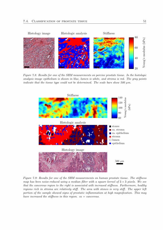
7.4. Classification of prostate tissue 51
You
ng’smodulus(kPa)
StiffnessHistologic analysisHistology image
20
40
60
80
Figure 7.8: Results for one of the SHM measurements on porcine prostate tissue. In the histologicanalysis image epithelium is shown in blue, lumen is white, and stroma is red. The gray pointsindicate that the tissue type could not be determined. The scale bars show 500 µm.
(kPa)
You
ng’smodulus
stones
ca. stroma
ca. epithelium
stroma
lumen
epithelium
500 µm
Stiffness
Histologic analysis
Histology image
60
80
100
120
140
Figure 7.9: Results for one of the SHM measurements on human prostate tissue. The stiffnessmap has been noise-reduced using a median filter with a square kernel of 3× 3 pixels. We seethat the cancerous region to the right is associated with increased stiffness. Furthermore, healthyregions rich in stroma are relatively stiff. The area with stones is very stiff. The upper leftportion of the sample showed signs of prostatic inflammation at high magnification. This mayhave increased the stiffness in this region. ca = cancerous.

52 General Results and Discussion
16541448
935
813
stroma (n=280)
lumen (n=41)
epithelium (n=900)
intensity
(arb)
Raman shift (cm−1)
600 800 1000 1200 1400 1600 1800
Figure 7.10: The mean spectra of the porcine tissue types. The largest differences were found atthe labeled peaks, which were all assigned to collagen (D).
distinguished from lumen and healthy epithelium (p < 0.05). This finding casts new lighton the possibilities for tissue characterization using TRM alone. There may be additionaldiagnostic value, besides the stiffness calculated from the slope of the measurement curve,in the raw data. Further studies are necessary to explain the origin of the nonlineareffects, and assess their possible diagnostic value.
The spectral quality of the RS measurements on human samples was low (D). Thereason was that the surgical margin of the removed prostate was covered with blue ink.This is standard clinical procedure; it is useful for determining if all cancerous tissuewas removed at radical prostatectomy [17]. If cancerous tissue is found to be in contactwith the inked margin, the patient is defined to have a positive surgical margin. The inkgave rise to very strong fluorescence that often saturated the detector in the Fingerprintinterval, and swamped the Raman signal from the tissue. Fortunately, it was possibleto partly overcome this problem by analyzing the high wavenumber region from 2400–3425 cm−1, where the fluorescence was decreased. Although this region does not containas much biochemical information as the Fingerprint region, the diagnostic value may besimilar [86–88]. We found that almost as high classification accuracies were attained forthe porcine samples using the high wavenumber region, as compared to the Fingerprintregion. However, in comparison with the spectra of porcine tissue the spectral qualitywas lower for human tissue in the high wavenumber region. Spectra of human tissue wereconsiderably more noisy. Thus, we believe that important diagnostic information mayhave been lost due to the strong fluorescence.
Figure 7.12 presents the SVM classification accuracies for distinguishing healthy porcinetissue types, and for distinguishing healthy and cancerous prostate tissue, for different

7.4. Classification of prostate tissue 53
stroma (n=161)
lumen (n=3)
epithelium (n=920)
frequency
shift(H
z)
indentation (µm)
0 2 4 6 8 10 12 14 16 18−160
−140
−120
−100
−80
−60
−40
−20
Figure 7.11: The mean SHM measurement curves, for points in homogeneous tissue regions, forthe different tissue types for one of the porcine samples. We see that the measurement curvesshow slight deviations from linearity, and that the curvature for stroma differs from epitheliumand lumen.
degrees of tissue homogeneity. TRM alone attained a high accuracy for distinguishingdifferent porcine tissue types, especially for the most homogeneous tissue regions whenit was 82%. In combination with RS the accuracy was > 80%, even when the mostheterogeneous tissue regions were included in the analysis. For differentiating canceroustissue the accuracy was 67–70% when using the TRM alone. The analysis of the SHMdata indicated that the overlapping stiffness distributions of healthy stroma and cancerousepithelium may have been the main limiting factor (D). The accuracy was increased to73–77% when RS was added to SHM. The combined accuracy would most likely haveincreased if the spectral quality for human tissue would have been higher. In futurestudies alternative experimental approaches should be considered, in order to eliminateor decrease the interference from the application of ink to the surface of the removedprostates.
The results of Papers C and D clearly show that it is feasible and valuable to combineTRM and RS for tissue characterization. Used as a research tool the combination showspromise to extract unknown relationships between stiffness and biochemical compositionby the multivariate approach presented in Paper C. This may help to explain the causefor changes in tissue stiffness due to cancer. For the development of a clinical instrumentfor probing surgical margins Paper D indicates that there is diagnostic information fordistinguishing healthy and cancerous tissue using TRM alone. With the addition of RSthe diagnostic power is increased. The combination shows high potential for exact tissuecharacterization, even in complex tissue regions with a mix of different tissue types. Thisis very promising for the development of a clinical tool to be used during PCa surgery.

54 General Results and Discussion
porcine tissue, SHM+RS
porcine tissue, SHM
human tissue, SHM+RS
human tissue, SHM
cross-validationaccuracy
(%)
tissue homogeneity threshold
> 50% > 66% > 83%
0
20
40
60
80
100
Figure 7.12: The five-fold cross-validation accuracies for SVM classification of the porcineprostate tissue types epithelium, lumen and stroma, and healthy and cancerous human prostatetissue.
Chapter 8
General Summary and Conclusions
This thesis reviewed the current state–of–the–art in PCa detection. The importance ofappropriate in vitro preparation protocols and measurement procedures was discussed andevaluated, and the effects of snap-freezing and NIR laser illumination on porcine prostatetissue were investigated using RS. The combination of TRM and RS was evaluated inexperiments on porcine and human tissues using multivariate techniques for explaining thedata correlation and assessing the potential for characterization of healthy and diseasedtissue.
From the review it was concluded that the specificity and sensitivity of clinical methodscurrently used for PCa detection and diagnosis, the PSA test and SB, are insufficient.Indolent and aggressive tumors cannot be reliably differentiated, which results in manymen being treated either unnecessarily or too late. Clinical benefits of state–of–the–arttechnology for PCa imaging, advanced ultrasound and MR techniques, have still notbeen convincingly shown. There is a need for complementary and cost-effective detectionmethods. TRM and RS are promising complementary techniques.
In the RS study no indications of tissue degradation due to 830 nm laser illumination atan irradiance of ∼ 3 · 1010 W m−2 were observed. Snap-freezing and subsequent storage at−80 ◦C gave rise to subtle but significant changes in the Raman spectra, most likely relatedto alterations in the protein conformations. Since the main changes in cancerous prostatetissue appear to be related to DNA and lipids, these findings indicate that snap-freezingmay be used to preserve samples for in vitro studies concerning PCa detection.
The measurements on porcine and human tissue types showed that the combined datacan be used to study the causes of differences in tissue stiffness through a multivariateapproach. Furthermore, the classification accuracy of healthy porcine tissue types was highusing TRM alone, and increased substantially when RS was added. The measurementson human tissue indicate that efficient detection of PCa may be possible.
To summarize, this thesis shows that a combined instrument incorporating bothTRM and RS is a promising complementary method for PCa detection. Snap-freezing ofsamples may be used in future RS evaluations of changes in cancerous prostate tissue.The instrument has potential for assisting surgeons in cancer surgery, and for biopsyguidance. The goal is to provide a more secure diagnosis and consequently more efficienttreatment of the patient.
55

56 General Summary and Conclusions

Chapter 9
Future Outlook
This thesis shows that a future instrument combining TRM and RS may be usefulfor tumor detection and diagnosis. The TRM sensor would be used to swiftly scan thetissue for stiff lesions. With the additional diagnostic power of RS it may be determinedif a lesion is benign or malign, and whether it is indolent or aggressive. This could beaccomplished in near real-time through computerized interpretation of measurement data.The combined instrument may be constructed by molding an RS fiber optic probe into acylindrical resonance sensor element, as depicted in Figure 9.1. This is the thought devicefor probing surgical margins. Since the RS probe is shielded from surrounding light bythe piezoelectric element, measurements may be performed in bright environments. TheTRM sensor can be used for tactile feedback to the surgeons and inform them when theinstrument touches the tissue. This would facilitate the practical clinical use.
A possible design for a miniaturized version of the combined instrument is shown inFigure 9.2. It uses a single optic fiber inserted into a hollow glass needle, as used for theMTS. This device could be used for possible guidance of prostate biopsies. By using RSmeasurements in the high wavenumber region it is possible to use a single optic fiber forspectral acquisition [86–88].
Although this thesis focused on PCa, the combined instrument could potentially beused for a variety of biomedical applications, both in vitro and in vivo. Both TRM andRS are versatile methods [18, 22], and the combination even more so, since biomechanicaland biochemical information are retrieved simultaneously.
57

58 Future Outlook
Fiber optic probe Cylindrical PZT element
Hemispherical tip
Quartz window
Rubber mount
Lens
Focal length
Figure 9.1: A possible design of an instrument for scanning of surgical margins.
Hemispherical tip
Single optic fiber
Glass needle
Figure 9.2: A possible design for a miniaturized instrument.

References
[1] J. Ferlay, D. M. Parkin, and E. Steliarova-Foucher, “Estimates of cancer incidenceand mortality in Europe in 2008”, Eur J Cancer, vol. 46, pp. 765–781, 2010.
[2] A. Jemal, R. Siegel, J. Xu, and E. Ward, “Cancer statistics, 2010”, CA Cancer JClin, vol. 60, pp. 277–300, 2010.
[3] S. A. Fedewa, R. Etzioni, W. D. Flanders, A. Jemal, and E. M. Ward, “Associa-tion of insurance and race/ethnicity with disease severity among men diagnosedwith prostate cancer, National Cancer Database 2004–2006”, Cancer EpidemiolBiomarkers Prev, vol. 19, pp. 2437–2444, 2010.
[4] N. J. Fitzsimons, L. Sun, and J. W. Moul, “Medical technologies for the diagnosisof prostate cancer”, Expert Rev Med Devices, vol. 4, pp. 227–239, 2007.
[5] J. Hegarty, P. V. Beirne, E. Walsh, H. Comber, T. Fitzgerald, and M. W. Kazer,“Radical prostatectomy versus watchful waiting for prostate cancer”, CochraneDatabase Syst Rev, no. CD006590 (67 pp.), 2010.
[6] J. E. Johansson, L. Holmberg, S. Johansson, R. Bergstrom, and H. O. Adami,“Fifteen-year survival in prostate cancer – A prospective, population-based study inSweden”, JAMA, vol. 277, pp. 467–471, 1997.
[7] H. Hricak, P. L. Choyke, S. C. Eberhardt, S. A. Leibel, and P. T. Scardino, “Imagingprostate cancer: A multidisciplinary perspective”, Radiology, vol. 243, pp. 28–53,2007.
[8] F. H. Schroder, J. Hugosson, M. J. Roobol, T. L. J. Tammela, S. Ciatto, V. Nelen,M. Kwiatkowski, M. Lujan, H. Lilja, M. Zappa, L. J. Denis, F. Recker, A. Berenguer,L. Maattanen, C. H. Bangma, G. Aus, A. Villers, X. Rebillard, T. van der Kwast,B. G. Blijenberg, S. M. Moss, H. J. de Koning, A. Auvinen, and E. R. S. P. C.Investigators, “Screening and prostate-cancer mortality in a randomized Europeanstudy”, N Engl J Med, vol. 360, pp. 1320–1328, 2009.
[9] D. C. Fernandez, R. Bhargava, S. M. Hewitt, and I. W. Levin, “Infrared spectroscopicimaging for histopathologic recognition”, Nat Biotechnol, vol. 23, pp. 469–474, 2005.
59

60 References
[10] J. E. McNeal, “Normal histology of the prostate”, Am J Surg Pathol, vol. 12,pp. 619–633, 1988.
[11] A. P. S. Kirkham, M. Emberton, and C. Allen, “How good is MRI at detectingand characterising cancer within the prostate?”, Eur Urol, vol. 50, pp. 1163–74;discussion 1175, 2006.
[12] L. Pallwein, M. Mitterberger, A. Pelzer, G. Bartsch, H. Strasser, G. M. Pinggera,F. Aigner, J. Gradl, D. Z. Nedden, and F. Frauscher, “Ultrasound of prostate cancer:recent advances”, Eur Radiol, vol. 18, pp. 707–715, 2008.
[13] M. Fuchsjager, A. Shukla-Dave, O. Akin, J. Barentsz, and H. Hricak, “Prostatecancer imaging”, Acta Radiol, vol. 49, pp. 107–120, 2008.
[14] C. Sumey and T. W. Flaig, “Adjuvant medical therapy for prostate cancer”, ExpertOpin Pharmacother, vol. 12, pp. 73–84, 2011.
[15] B. Tareen, J. Kimmel, and W. C. Huang, “Contemporary treatment of high-risklocalized prostate cancer”, Expert Rev Anticancer Ther, vol. 10, pp. 1069–1076,2010.
[16] Y. Yang, “Treatment of the positive surgical margin following radical prostatectomy”,Chin Med J, vol. 121, pp. 375–379, 2008.
[17] O. Yossepowitch, A. Bjartell, J. A. Eastham, M. Graefen, B. D. Guillonneau, P. I.Karakiewicz, R. Montironi, and F. Montorsi, “Positive surgical margins in radicalprostatectomy: outlining the problem and its long-term consequences”, Eur Urol,vol. 55, pp. 87–99, 2009.
[18] O. A. Lindahl, C. E. Constantinou, A. Eklund, Y. Murayama, P. Hallberg, andS. Omata, “Tactile resonance sensors in medicine”, J Med Eng Technol, vol. 33,pp. 263–273, 2009.
[19] V. Jalkanen, B. M. Andersson, A. Bergh, B. Ljungberg, and O. A. Lindahl, “Res-onance sensor measurements of stiffness variations in prostate tissue in vitro – aweighted tissue proportion model”, Physiol Meas, vol. 27, pp. 1373–1386, 2006.
[20] V. Jalkanen, B. M. Andersson, A. Bergh, B. Ljungberg, and O. A. Lindahl, “Prostatetissue stiffness as measured with a resonance sensor system: a study on silicone andhuman prostate tissue in vitro”, Med Biol Eng Comput, vol. 44, pp. 593–603, 2006.
[21] V. Jalkanen, B. M. Andersson, A. Bergh, B. Ljungberg, and O. A. Lindahl, “Spatialvariations in prostate tissue histology as measured by a tactile resonance sensor”,Physiol Meas, vol. 28, pp. 1267–1281, 2007.
[22] C. Krafft, G. Steiner, C. Beleites, and R. Salzer, “Disease recognition by infraredand Raman spectroscopy”, J Biophotonics, vol. 2, pp. 13–28, 2009.
References 61
[23] M. D. Keller, E. M. Kanter, and A. Mahadevan-Jansen, “Raman spectroscopy forcancer diagnosis”, Spectroscopy, vol. 21, pp. 33–41, 2006.
[24] P. Crow, N. Stone, C. A. Kendall, J. S. Uff, J. A. M. Farmer, H. Barr, andM. P. J. Wright, “The use of Raman spectroscopy to identify and grade prostaticadenocarcinoma in vitro”, Br J Cancer, vol. 89, pp. 106–108, 2003.
[25] P. Crow, B. Barrass, C. Kendall, M. Hart-Prieto, M. Wright, R. Persad, andN. Stone, “The use of Raman spectroscopy to differentiate between different prostaticadenocarcinoma cell lines”, Br J Cancer, vol. 92, pp. 2166–2170, 2005.
[26] P. Crow, A. Molckovsky, N. Stone, J. Uff, B. Wilson, and L.-M. WongKeeSong,“Assessment of fiberoptic near-infrared Raman spectroscopy for diagnosis of bladderand prostate cancer”, Urology, vol. 65, pp. 1126–1130, 2005.
[27] N. Stone, M. C. H. Prieto, P. Crow, J. Uff, and A. W. Ritchie, “The use of Ramanspectroscopy to provide an estimation of the gross biochemistry associated withurological pathologies”, Anal Bioanal Chem, vol. 387, pp. 1657–1668, 2007.
[28] A. Nijssen, S. Koljenovic, T. C. B. Schut, P. J. Caspers, and G. J. Puppels, “Towardsoncological application of Raman spectroscopy”, J Biophotonics, vol. 2, pp. 29–36,2009.
[29] S. Devpura, J. S. Thakur, F. H. Sarkar, W. A. Sakr, V. M. Naik, and R. Naik,“Detection of benign epithelia, prostatic intraepithelial neoplasia, and cancer regionsin radical prostatectomy tissues using Raman spectroscopy”, Vib Spectrosc, vol. 53,pp. 227–232, 2010.
[30] P. Matousek, “Deep non-invasive Raman spectroscopy of living tissue and powders”,Chem Soc Rev, vol. 36, pp. 1292–1304, 2007.
[31] G. J. Tortora and B. Derrickson, Principles of Anatomy and Physiology. New York:Wiley & Sons, 11 ed., 2006.
[32] S. N. Rasmussen and P. Riis, “Rectal wall thickness measured by ultrasound inchronic inflammatory diseases of the colon”, Scand J Gastroenterol, vol. 20, pp. 109–114, 1985.
[33] G. R. Cunha, A. A. Donjacour, P. S. Cooke, S. Mee, R. M. Bigsby, S. J. Higgins,and Y. Sugimura, “The endocrinology and developmental biology of the prostate”,Endocr Rev, vol. 8, pp. 338–362, 1987.
[34] L. C. Costello and R. B. Franklin, “Prostatic fluid electrolyte composition for thescreening of prostate cancer: a potential solution to a major problem”, ProstateCancer Prostatic Dis, vol. 12, pp. 17–24, 2009.
[35] R. Klimas, B. Bennett, and W. A. Gardner, “Prostatic calculi: a review”, Prostate,vol. 7, pp. 91–96, 1985.

62 References
[36] J. D. Christian, T. C. Lamm, J. F. Morrow, and D. G. Bostwick, “Corpora amylaceain adenocarcinoma of the prostate: incidence and histology within needle corebiopsies”, Mod Pathol, vol. 18, pp. 36–39, 2005.
[37] A. Eklund, A. Bergh, and O. A. Lindahl, “A catheter tactile sensor for measuringhardness of soft tissue: measurement in a silicone model and in an in vitro humanprostate model”, Med Biol Eng Comput, vol. 37, pp. 618–624, 1999.
[38] M. Swindle and A. Smith, “Comparative anatomy and physiology of the pig”, ScandJ Lab Anim Sci, vol. 25, pp. 11–21, 1998.
[39] R. N. C. Aitken, “A histochemical study of the accessory genital glands of the boar”,J Anat, vol. 94, pp. 130–142, 1960.
[40] M. Nicaise, H. Lauwers, and P. Simoens, “Morphological study of the development ofthe disseminate prostate in intact and castrated male pigs aged two to six months”,Acta Anat, vol. 141, pp. 335–347, 1991.
[41] F. Bray, J. Lortet-Tieulent, J. Ferlay, D. Forman, and A. Auvinen, “Prostate cancerincidence and mortality trends in 37 European countries: an overview”, Eur JCancer, vol. 46, pp. 3040–3052, 2010.
[42] D. E. Neal, H. Y. Leung, P. H. Powell, F. C. Hamdy, and J. L. Donovan, “Unansweredquestions in screening for prostate cancer”, Eur J Cancer, vol. 36, pp. 1316–1321,2000.
[43] M. Yin, S. Bastacky, U. Chandran, M. J. Becich, and R. Dhir, “Prevalence ofincidental prostate cancer in the general population: a study of healthy organdonors”, J Urol, vol. 179, pp. 892–895; discussion 895, 2008.
[44] V. Kundra, “Prostate cancer imaging”, Semin Roentgenol, vol. 41, pp. 139–149,2006.
[45] J. E. McNeal, E. A. Redwine, F. S. Freiha, and T. A. Stamey, “Zonal distributionof prostatic adenocarcinoma – Correlation with histologic pattern and direction ofspread”, Am J Surg Pathol, vol. 12, pp. 897–906, 1988.
[46] A. E. Pelzer, J. Bektic, A. P. Berger, E. J. Halpern, F. Koppelstatter, A. Klauser,P. Rehder, W. Horninger, G. Bartsch, and F. Frauscher, “Are transition zonebiopsies still necessary to improve prostate cancer detection? Results from the Tyrolscreening project”, Eur Urol, vol. 48, pp. 916–21; discussion 921, 2005.
[47] E. J. Halpern, “Contrast-enhanced ultrasound imaging of prostate cancer”, RevUrol, vol. 8, pp. S29–S37, 2006.
[48] R. C. Flanigan, W. J. Catalona, J. P. Richie, F. R. Ahmann, M. A. Hudson, P. T.Scardino, J. B. deKernion, T. L. Ratliff, L. R. Kavoussi, and B. L. Dalkin, “Accuracy

References 63
of digital rectal examination and transrectal ultrasonography in localizing prostatecancer”, J Urol, vol. 152, pp. 1506–1509, 1994.
[49] W. L. Valk and W. K. Mebust, “The management of the prostatic nodule”, JAMA,vol. 209, p. 1697, 1969.
[50] J. C. Applewhite, B. R. Matlaga, D. L. McCullough, and M. C. Hall, “Transrectalultrasound and biopsy in the early diagnosis of prostate cancer”, Cancer Control,vol. 8, pp. 141–150, 2001.
[51] G. D. Angelis, H. G. Rittenhouse, S. D. Mikolajczyk, L. B. Shamel, and A. Semjonow,“Twenty Years of PSA: From Prostate Antigen to Tumor Marker”, Rev Urol, vol. 9,pp. 113–123, 2007.
[52] I. M. Thompson, D. K. Pauler, P. J. Goodman, C. M. Tangen, M. S. Lucia,H. L. Parnes, L. M. Minasian, L. G. Ford, S. M. Lippman, E. D. Crawford, J. J.Crowley, and C. A. Coltman, “Prevalence of prostate cancer among men with aprostate-specific antigen level < or = 4.0 ng per milliliter”, N Engl J Med, vol. 350,pp. 2239–2246, 2004.
[53] G. L. Andriole, R. L. Grubb, S. S. Buys, D. Chia, T. R. Church, M. N. Fouad,E. P. Gelmann, P. A. Kvale, D. J. Reding, J. L. Weissfeld, L. A. Yokochi, E. D.Crawford, B. O’Brien, J. D. Clapp, J. M. Rathmell, T. L. Riley, R. B. Hayes, B. S.Kramer, G. Izmirlian, A. B. Miller, P. F. Pinsky, P. C. Prorok, J. K. Gohagan,C. D. Berg, and P. L. C. O. Project Team, “Mortality results from a randomizedprostate-cancer screening trial”, N Engl J Med, vol. 360, pp. 1310–1319, 2009.
[54] G. Draisma, R. Boer, S. J. Otto, I. W. van der Cruijsen, R. A. M. Damhuis, F. H.Schroder, and H. J. de Koning, “Lead times and overdetection due to prostate-specific antigen screening: estimates from the European Randomized Study ofScreening for Prostate Cancer”, J Natl Cancer Inst, vol. 95, pp. 868–878, 2003.
[55] R. Montironi, R. Mazzuccheli, M. Scarpelli, A. Lopez-Beltran, G. Fellegara, andF. Algaba, “Gleason grading of prostate cancer in needle biopsies or radical prostate-ctomy specimens: contemporary approach, current clinical significance and sourcesof pathology discrepancies”, BJU Int, vol. 95, pp. 1146–1152, 2005.
[56] R. Montironi, R. Mazzucchelli, and T. Kwast, “Morphological assessment of radi-cal prostatectomy specimens. A protocol with clinical relevance”, Virchows Arch,vol. 442, pp. 211–217, 2003.
[57] M. Seitz, F. Strittmatter, A. Roosen, D. Tilki, and C. Gratzke, “Current statusof ultrasound imaging in prostate cancer”, Panminerva Med, vol. 52, pp. 189–194,2010.
[58] S. Verma and A. Rajesh, “A clinically relevant approach to imaging prostate cancer:review”, AJR Am J Roentgenol, vol. 196, pp. S1–S10, 2011.

64 References
[59] C. R. Porter, K. Kodama, R. P. Gibbons, R. Correa, F. K.-H. Chun, P. Perrotte,and P. I. Karakiewicz, “25-year prostate cancer control and survival outcomes: a40-year radical prostatectomy single institution series”, J Urol, vol. 176, pp. 569–574,2006.
[60] R. F. Coelho, B. Rocco, M. B. Patel, M. A. Orvieto, S. Chauhan, V. Ficarra,S. Melegari, K. J. Palmer, and V. R. Patel, “Retropubic, laparoscopic, and robot-assisted radical prostatectomy: a critical review of outcomes reported by high-volumecenters”, J Endourol, vol. 24, pp. 2003–2015, 2010.
[61] I. Singh and A. K. Hemal, “Robotic-assisted radical prostatectomy in 2010”, ExpertRev Anticancer Ther, vol. 10, pp. 671–682, 2010.
[62] T. H. V. der Kwast, M. Bolla, H. V. Poppel, P. V. Cangh, K. Vekemans, L. D. Pozzo,J.-F. Bosset, K. H. Kurth, F. H. Schroder, and L. Collette, “Identification of pa-tients with prostate cancer who benefit from immediate postoperative radiotherapy:EORTC 22911”, J Clin Oncol, vol. 25, pp. 4178–4186, 2007.
[63] A. N. Vis, F. H. Schroder, and T. H. van der Kwast, “The actual value of thesurgical margin status as a predictor of disease progression in men with earlyprostate cancer”, Eur Urol, vol. 50, pp. 258–265, 2006.
[64] J. Thoms, J. S. Goda, A. R. Zlotta, N. E. Fleshner, T. H. van der Kwast, S. Supiot,P. Warde, and R. G. Bristow, “Neoadjuvant radiotherapy for locally advanced andhigh-risk prostate cancer”, Nat Rev Clin Oncol, vol. 8, pp. 107–113, 2011.
[65] T. Ikeda, Fundamentals of Piezoelectricity. Oxford: Oxford University Press, 1990.
[66] F. Mandl, Statistical Physics. Chichester: John Wiley & Sons, 2 ed., 1988.
[67] S. Omata and Y. Terunuma, “New tactile sensor like the human hand and itsapplications”, Sensor Actuat A, vol. 35, pp. 9–15, 1992.
[68] Y. Murayama and S. Omata, “Fabrication of micro tactile sensor for the mea-surement of micro-scale local elasticity”, Sensor Actuat A, vol. 109, pp. 202–207,2004.
[69] G. Gladwell and C. Kleesattel, “The contact impedance meter I”, Ultrasonics, vol. 6,pp. 175–180, 1968.
[70] G. Gladwell and C. Kleesattel, “The contact impedance meter II”, Ultrasonics,vol. 6, pp. 244–252, 1968.
[71] V. Jalkanen, B. M. Andersson, A. Bergh, B. Ljungberg, and O. A. Lindahl, “Ex-planatory models for a tactile resonance sensor system – elastic and density-relatedvariations of prostate tissue in vitro”, Physiol Meas, vol. 29, pp. 729–745, 2008.

References 65
[72] Y. Murayama, C. E. Constantinou, and S. Omata, “Remote sensing of mechanicalproperties of materials using a novel ultrasound transducer and signal processing”,IEEE Trans Ultrason Ferroelectr Freq Control, vol. 52, pp. 439–444, 2005.
[73] Y. Murayama, M. Haruta, Y. Hatakeyama, T. Shiina, H. Sakuma, S. Takenoshita,S. Omata, and C. E. Constantinou, “Development of a new instrument for exami-nation of stiffness in the breast using haptic sensor technology”, Sensor Actuat A,vol. 143, pp. 430–438, 2008.
[74] V. Jalkanen, “Hand-held resonance sensor for tissue stiffness measurements: atheoretical and experimental analysis”, Meas Sci Technol, vol. 21, 055801 (8 pp.),2010.
[75] Y. Murayama, S. Omata, T. Yajima, Q. Peng, K. Shishido, D. M. Peehl, andC. E. Constantinou, “High Resolution Regional Elasticity Mapping of the HumanProstate”, in Proceedings of the 29th Annual International Conference of the IEEEEMBS. Cite Internationale, Lyon, France. August 23-26, 2007, pp. 5802–5805, 2007.
[76] E. Smith and G. Dent, Modern Raman Spectroscopy: A Practical Approach. Chich-ester: John Wiley & Sons, 2005.
[77] V. Tuchin, Tissue Optics - Light Scattering Methods and Instruments for MedicalDiagnosis. Bellingham: SPIE Press, 2 ed., 2007.
[78] D. A. Long, “80th Anniversary of the discovery of the Raman Effect: a celebration”,J Raman Spectrosc, vol. 39, pp. 316–321, 2008.
[79] C. V. Raman and K. S. Krishnan, “A new type of secondary radiation”, Nature,vol. 121, pp. 501–502, 1928.
[80] J. R. Ferraro, K. Nakamoto, and C. W. Brown, Introductory Raman Spectroscopy.San Diego: Academic Press, 2 ed., 2003.
[81] A. Mahadevan-Jansen and R. R. Richards-Kortum, “Raman spectroscopy for thedetection of cancers and precancers”, J Biomed Opt, vol. 1, pp. 31–70, 1996.
[82] G. Pitt, D. Batchelder, R. Bennett, R. Bormett, I. Hayward, B. Smith, K. Williams,Y. Yang, K. Baldwin, and S. Webster, “Engineering aspects and applications of thenew Raman instrumentation”, IEE Proc-Sci Meas Technol, vol. 152, pp. 241–318,2005.
[83] E. B. Hanlon, R. Manoharan, T.-W. Koo, K. E. Shafer, J. T. Motz, M. Fitzmaurice,J. R. Kramer, I. Itzkan, R. R. Dasari, and M. S. Feld, “Topical review: prospectsfor in vivo Raman spectroscopy”, Phys Med Biol, vol. 45, pp. R1–R59, 2000.
[84] J. C. C. Day, R. Bennett, B. Smith, C. Kendall, J. Hutchings, G. M. Meaden,C. Born, S. Yu, and N. Stone, “A miniature confocal Raman probe for endoscopicuse”, Phys Med Biol, vol. 54, pp. 7077–7087, 2009.
66 References
[85] C. Kendall, J. Day, J. Hutchings, B. Smith, N. Shepherd, H. Barr, and N. Stone,“Evaluation of Raman probe for oesophageal cancer diagnostics”, Analyst, vol. 135,pp. 3038–3041, 2010.
[86] S. Koljenovic, T. C. B. Schut, R. Wolthuis, B. de Jong, L. Santos, P. J. Caspers,J. M. Kros, and G. J. Puppels, “Tissue characterization using high wave numberRaman spectroscopy”, J Biomed Opt, vol. 10, 031116 (11 pp.), 2005.
[87] L. F. Santos, R. Wolthuis, S. Koljenovic, R. M. Almeida, and G. J. Puppels, “Fiber-optic probes for in vivo Raman spectroscopy in the high-wavenumber region”, AnalChem, vol. 77, pp. 6747–6752, 2005.
[88] S. Koljenovic, T. C. B. Schut, R. Wolthuis, A. J. P. E. Vincent, G. Hendriks-Hagevi,L. Santos, J. M. Kros, and G. J. Puppels, “Raman spectroscopic characterization ofporcine brain tissue using a single fiber-optic probe”, Anal Chem, vol. 79, pp. 557–564, 2007.
[89] Y. Komachi, H. Sato, K. Aizawa, and H. Tashiro, “Micro-optical fiber probe for usein an intravascular Raman endoscope”, Appl Opt, vol. 44, pp. 4722–4732, 2005.
[90] Y. Komachi, H. Sato, and H. Tashiro, “Intravascular Raman spectroscopic catheterfor molecular diagnosis of atherosclerotic coronary disease”, Appl Opt, vol. 45,pp. 7938–7943, 2006.
[91] Y. Komachi, T. Katagiri, H. Sato, and H. Tashiro, “Improvement and analysis of amicro Raman probe”, Appl Opt, vol. 48, pp. 1683–1696, 2009.
[92] Y. Hattori, Y. Komachi, T. Asakura, T. Shimosegawa, G.-I. Kanai, H. Tashiro,and H. Sato, “In vivo Raman study of the living rat esophagus and stomach usinga micro-Raman probe under an endoscope”, Appl Spectrosc, vol. 61, pp. 579–584,2007.
[93] N. Stone and P. Matousek, “Advanced transmission Raman spectroscopy: a promis-ing tool for breast disease diagnosis”, Cancer Res, vol. 68, pp. 4424–4430, 2008.
[94] H. Edwards and E. Carter, “Biological Applications of Raman Spectroscopy”,in Infrared and Raman Spectroscopy of Biological Materials (H.-U. Gremlich andB. Yan, eds.), vol. 24 of Practical Spectroscopy, ch. 11, New York: Marcel Dekker,2001.
[95] L. C. Kwek, S. Fu, T. C. Chia, C. H. Diong, C. L. Tang, and S. M. Krishnan, “High-sensitivity and specificity of laser-induced autofluorescence spectra for detection ofcolorectal cancer with an artificial neural network”, Appl Opt, vol. 44, pp. 4004–4008,2005.
[96] C. A. Lieber and A. Mahadevan-Jansen, “Automated method for subtraction offluorescence from biological Raman spectra”, Appl Spectrosc, vol. 57, pp. 1363–1367,2003.

References 67
[97] A. Cao, A. K. Pandya, G. K. Serhatkulu, R. E. Weber, H. Dai, J. S. Thakur, V. M.Naik, R. Naik, G. W. Auner, R. Rabah, and D. C. Freeman, “A robust methodfor automated background subtraction of tissue fluorescence”, J Raman Spectrosc,vol. 38, pp. 1199–1205, 2007.
[98] Z. Movasaghi, S. Rehman, and I. Rehman, “Raman spectroscopy of biologicaltissues”, Appl Spectrosc Rev, vol. 42, pp. 493–541, 2007.
[99] A. Taleb, J. Diamond, J. J. McGarvey, J. R. Beattie, C. Toland, and P. W. Hamilton,“Raman microscopy for the chemometric analysis of tumor cells”, J Phys Chem B,vol. 110, pp. 19625–19631, 2006.
[100] N. Stone, C. Kendall, N. Shepherd, P. Crow, and H. Barr, “Near-infrared Ramanspectroscopy for the classification of epithelial pre-cancers and cancers”, J RamanSpectrosc, vol. 33, pp. 564–573, 2002.
[101] P. Crow, A. Ritchie, M. Wright, C. Kendall, and N. Stone, “Evaluation of Ramanspectroscopy to provide a real time optical method for discrimination betweennormal and abnormal tissue in the prostate”, Eur Urol Suppl, vol. 1, p. 92, 2002.
[102] M. G. Shim and B. C. Wilson, “The effects of ex vivo handling procedures on thenear-infrared Raman spectra of normal mammalian tissues”, Photochem Photobiol,vol. 63, pp. 662–671, 1996.
[103] C. M. Krishna, G. D. Sockalingum, B. M. Vadhiraja, K. Maheedhar, A. C. K. Rao,L. Rao, L. Venteo, M. Pluot, D. J. Fernandes, M. S. Vidyasagar, V. B. Kartha,and M. Manfait, “Vibrational spectroscopy studies of formalin-fixed cervix tissues”,Biopolymers, vol. 85, pp. 214–221, 2007.
[104] C. M. Krishna, G. D. Sockalingum, L. Venteo, R. A. Bhat, P. Kushtagi, M. Pluot,and M. Manfait, “Evaluation of the suitability of ex vivo handled ovarian tissues foroptical diagnosis by Raman microspectroscopy”, Biopolymers, vol. 79, pp. 269–276,2005.
[105] E. O Faolain, M. B. Hunter, J. M. Byrne, P. Kelehan, M. McNamara, H. J. Byrne,and F. M. Lyng, “A study examining the effects of tissue processing on humantissue sections using vibrational spectroscopy”, Vib Spectrosc, vol. 38, pp. 121–127,2005.
[106] N. Boustany, J. Crawford, R. Manoharan, R. Dasari, and M. Feld, “Effects offreeze-thaw and photobleaching on the ultraviolet resonance Raman spectra ofhuman colon biopsies”, Appl Spectrosc, vol. 55, pp. 1506–1513, 2001.
[107] K. C. Neuman, E. H. Chadd, G. F. Liou, K. Bergman, and S. M. Block, “Charac-terization of photodamage to escherichia coli in optical traps”, Biophys J, vol. 77,pp. 2856–2863, 1999.

68 References
[108] I. Notingher, S. Verrier, H. Romanska, A. Bishop, J. Polak, and L. Hench, “Insitu characterisation of living cells by Raman spectroscopy”, Spectroscopy, vol. 16,pp. 43–51, 2002.
[109] G. J. Puppels, J. H. Olminkhof, G. M. Segers-Nolten, C. Otto, F. F. de Mul, andJ. Greve, “Laser irradiation and Raman spectroscopy of single living cells andchromosomes: sample degradation occurs with 514.5 nm but not with 660 nm laserlight”, Exp Cell Res, vol. 195, pp. 361–367, 1991.
[110] R. W. Chan and I. R. Titze, “Effect of postmortem changes and freezing on theviscoelastic properties of vocal fold tissues”, Ann Biomed Eng, vol. 31, pp. 482–491,2003.
[111] M. Szarko, K. Muldrew, and J. E. Bertram, “Freeze-thaw treatment effects on thedynamic mechanical properties of articular cartilage”, BMC Musculoskelet Disord,vol. 11, 231 (8 pp.), 2010.
[112] S. Krag and T. T. Andreassen, “Effect of freezing on lens capsule mechanicalbehavior”, Ophthalmic Res, vol. 30, pp. 280–285, 1998.
[113] T. Oie, H. Suzuki, T. Fukuda, Y. Murayama, S. Omata, K. Kanda, and Y. Nakayama,“Tactile Mapping System: A Novel Imaging Technology for Surface Topography andElasticity of Tissues or Organs”, Innovations, vol. 4, pp. 345–350, 2009.
[114] T. Oie, Y. Murayama, T. Fukuda, C. Nagai, S. Omata, K. Kanda, H. Yaku, andY. Nakayama, “Local elasticity imaging of vascular tissues using a tactile mappingsystem”, J Artif Organs, vol. 12, pp. 40–46, 2009.
[115] T. Oie, H. Suzuki, Y. Murayama, T. Fukuda, S. Omata, K. Kanda, K. Takamizawa,and Y. Nakayama, “Surface elasticity imaging of vascular tissues in a liquid envi-ronment by a scanning haptic microscope”, J Artif Organs, vol. 13, pp. 121–125,2010.
[116] R. A. Johnson and D. W. Wichern, Applied Multivariate Statistical Analysis. UpperSaddle River: Prentice-Hall, 4 ed., 1998.
[117] M. Romeo and M. Diem, “Infrared spectral imaging of lymph nodes: Strategies foranalysis and artifact reduction”, Vib Spectrosc, vol. 38, pp. 115–119, 2005.
[118] C. Cortes and V. Vapnik, “Support-Vector Networks”, Machine Learning, vol. 20,pp. 273–297, 1995.
[119] Y.-W. Chen and C.-J. Lin, “Combining SVMs with Various Feature SelectionStrategies”, in Feature Extraction (I. Guyon, M. Nikravesh, S. Gunn, and L. Zadeh,eds.), vol. 207 of Studies in Fuzziness and Soft Computing, pp. 315–324, SpringerBerlin / Heidelberg, 2006.

References 69
[120] C.-W. Hsu and C.-J. Lin, “A Comparison of Methods for Multiclass Support VectorMachines”, IEEE T Neural Networ, vol. 13, pp. 415–425, 2002.
[121] M. Sattlecker, C. Bessant, J. Smith, and N. Stone, “Investigation of support vectormachines and Raman spectroscopy for lymph node diagnostics”, Analyst, vol. 135,pp. 895–901, 2010.
[122] E. Widjaja, W. Zheng, and Z. Huang, “Classification of colonic tissues using near-infrared Raman spectroscopy and support vector machines”, Int J Oncol, vol. 32,pp. 653–662, 2008.
[123] S. K. Majumder, N. Ghosh, and P. K. Gupta, “Support vector machine for opticaldiagnosis of cancer”, J Biomed Opt, vol. 10, 024034 (14 pp.), 2005.
[124] Y. Murayama, C. Constantinou, and S. Omata, “Development of Tactile Mappingsystem for the stiffness characterization of tissue slice using novel tactile sensingtechnology”, Sensor Actuat A, vol. 120, pp. 543–549, 2005.
[125] Y. Murayama and S. Omata, “Considerations in the design and sensitivity opti-mization of the micro tactile sensor”, IEEE Trans Ultrason Ferroelectr Freq Control,vol. 52, pp. 434–438, 2005.
[126] P. H. Eilers, “A perfect smoother”, Anal Chem, vol. 75, pp. 3631–3636, 2003.
[127] Y. L. Loethen, D. Zhang, R. N. Favors, S. B. G. Basiaga, and D. Ben-Amotz, “Second-derivative variance minimization method for automated spectral subtraction”, ApplSpectrosc, vol. 58, pp. 272–278, 2004.
[128] S. Kim, “A practical solution to the multivariate Behrens-Fisher problem”,Biometrika, vol. 79, pp. 171–176, 1992.
[129] L. M. Lix, H. J. Keselman, and A. M. Hinds, “Robust tests for the multivariateBehrens-Fisher problem”, Comput Methods Programs Biomed, vol. 77, pp. 129–139,2005.
[130] K. K. Yuen, “The two-sample trimmed t for unequal population variances”,Biometrika, vol. 61, pp. 165–171, 1974.
[131] S. W. T. P. J. Heijmink, H. van Moerkerk, L. A. L. M. Kiemeney, J. A. Witjes,F. Frauscher, and J. O. Barentsz, “A comparison of the diagnostic performanceof systematic versus ultrasound-guided biopsies of prostate cancer”, Eur Radiol,vol. 16, pp. 927–938, 2006.
[132] L. Pallwein, M. Mitterberger, J. Gradl, F. Aigner, W. Horninger, H. Strasser,G. Bartsch, D. zur Nedden, and F. Frauscher, “Value of contrast-enhanced ultra-sound and elastography in imaging of prostate cancer”, Curr Opin Urol, vol. 17,pp. 39–47, 2007.

70 References
[133] J. Kurhanewicz, D. Vigneron, P. Carroll, and F. Coakley, “Multiparametric magneticresonance imaging in prostate cancer: present and future”, Curr Opin Urol, vol. 18,pp. 71–77, 2008.
[134] P. Wang, Y. min Guo, M. Liu, Y. qian Qiang, X. juan Guo, Y. li Zhang, X.-Y.Duan, Q.-J. Zhang, and W. Liang, “A meta-analysis of the accuracy of prostatecancer studies which use magnetic resonance spectroscopy as a diagnostic tool”,Korean J Radiol, vol. 9, pp. 432–438, 2008.
[135] M. Chen, H.-D. Dang, J.-Y. Wang, C. Zhou, S.-Y. Li, W.-C. Wang, W.-F. Zhao,Z.-H. Yang, C.-Y. Zhong, and G.-Z. Li, “Prostate cancer detection: comparisonof T2-weighted imaging, diffusion-weighted imaging, proton magnetic resonancespectroscopic imaging, and the three techniques combined”, Acta Radiol, vol. 49,pp. 602–610, 2008.
[136] T. Hambrock, J. J. Fuetterer, H. J. Huisman, C. Hulsbergen-vandeKaa, J.-P. vanBasten, I. van Oort, J. A. Witjes, and J. O. Barentsz, “Thirty-two-channel coil 3Tmagnetic resonance-guided biopsies of prostate tumor suspicious regions identifiedon multimodality 3T magnetic resonance imaging: Technique and feasibility”, InvestRadiol, vol. 43, pp. 686–694, 2008.
[137] T. Tamada, T. Sone, Y. Jo, A. Yamamoto, T. Yamashita, N. Egashira, S. Imai, andM. Fukunaga, “Prostate cancer: relationships between postbiopsy hemorrhage andtumor detectability at MR diagnosis”, Radiology, vol. 248, pp. 531–539, 2008.
[138] K. J. Macura, “Multiparametric magnetic resonance imaging of the prostate: currentstatus in prostate cancer detection, localization, and staging”, Semin Roentgenol,vol. 43, pp. 303–313, 2008.
[139] J. M. Berg, J. L. Tymoczko, and L. Stryer, Biochemistry. New York: Freeman,5 ed., 2002.

Part II
71

72
Paper A
Technologies for localization anddiagnosis of prostate cancer
Authors:Stefan Candefjord, Kerstin Ramser and Olof A. Lindahl
Paper originally published in:Journal of Medical Engineering & Technology, vol. 33, pp. 585–603, 2009.1
© 2009 Informa Healthcare. Reproduced with permission.
1http://dx.doi.org/10.3109/03091900903111966
73

74

Review
Technologies for localization and diagnosis of prostate cancer
S. CANDEFJORD*{{, K. RAMSER{{ and O. A. LINDAHL{{
{Department of Computer Science and Electrical Engineering, Lulea University of Technology,971 87 Lulea, Sweden
{Centre for Biomedical Engineering and Physics, Lulea University of Technology
The gold standard for detecting prostate cancer (PCa), systematic biopsy, lacks sensitivity
as well as grading accuracy. PSA screening leads to over-treatment of many men, and it is
unclear whether screening reduces PCa mortality. This review provides an understanding
of the difficulties of localizing and diagnosing PCa. It summarizes recent developments of
ultrasound (including elastography) and MRI, and discusses some alternative experi-
mental techniques, such as resonance sensor technology and vibrational spectroscopy. A
comparison between the different methods is presented. It is concluded that new
ultrasound techniques are promising for targeted biopsy procedures, in order to detect
more clinically significant cancers while reducing the number of cores. MRI advances are
very promising, but MRI remains expensive and MR-guided biopsy is complex.
Resonance sensor technology and vibrational spectroscopy have shown promising results
in vitro. There is a need for large prospective multicentre trials that unambiguously prove
the clinical benefits of these new techniques.
Keywords: Prostate cancer; Imaging; Diagnosing; Grading; Targeted biopsy
List of abbreviations
ADC apparent diffusion coefficient
AUC area under receiver operating
characteristic curve
BPH benign prostatic hyperplasia
CDU colour Doppler ultrasound
CE contrast-enhanced
CHI continuous harmonic imaging
CZ central zone
DCE-MRI dynamic contrast-enhanced MRI
DRE digital rectal examination
DU Doppler ultrasound
DWI diffusion-weighted imaging
FTIR Fourier transform infrared spectroscopy
GS Gleason score
IHI intermittent harmonic imaging
IR infrared
MR magnetic resonance
MRI magnetic resonance imaging
MRSI magnetic resonance spectroscopic
imaging
PCa prostate cancer
PDU power Doppler ultrasound
PSA prostate-specific antigen
PZ peripheral zone
RS Raman spectroscopy
SB systematic biopsy
T1W T1-weighted
T2W T2-weighted
TNM tumour-node-metastasis
TRUS transrectal ultrasound
TZ transitional zone
VS vibrational spectroscopy
*Corresponding author. Email: [email protected]
Journal of Medical Engineering & Technology, 2009, 1–19, iFirst article
Journal of Medical Engineering & TechnologyISSN 0309-1902 print/ISSN 1464-522X online ª 2009 Informa UK Ltd.
http://www.informaworld.com/journalsDOI: 10.1080/03091900903111966
Downloaded By: [Candefjord, S.] At: 08:19 16 September 2009

1. Introduction
Prostate cancer (PCa) has the highest incidence of all
cancers, excluding nonmelanoma skin cancers, and is the
third leading cause of cancer-related death after lung and
colorectal cancer in European men [1]. Due to the ageing
population the prevalence of the disease is expected to
increase [2], and since 1995 the number of deaths caused by
PCa has increased by 16% [1]. Clinically significant PCa is
still much more common in Western countries than in Asia
[3], although the incidence of PCa observed at autopsy is
similar worldwide [4]. However, PCa mortality rates in Asia
are rising, which may be explained by gradual Westerniza-
tion and loss of protective cultural factors such as diet [3].
The gold standard for PCa detection and diagnosis, the
prostate-specific antigen (PSA) test and systematic biopsy
(SB), has many limitations, and fails to reveal a large
percentage of clinically significant tumours [5–7]. To reduce
PCa mortality and choose an appropriate therapy, new
imaging modalities and diagnostic tools are needed that can
accurately localize and diagnose PCa at an early stage [8].
To our knowledge recent reviews in the area have focused
on either a specific technology [9–11] or on biomarkers,
such as PSA [2, 12, 13]. Furthermore, the area of PCa
detection is constantly under debate, and new technologies
are emerging and established ones are improved. Therefore,
the aim of this review is to give a broad perspective on
current state-of-the-art techniques for PCa detection and
diagnosis in clinical use today and to mention promising
novelties. The review focuses on technical methods that
can, or have the potential to, directly localize/diagnose PCa
in situ via non-invasive or minimally invasive routes.
Methods that label the tumour, e.g. with radioactive or
fluorescent markers, are excluded. The included methods
are ultrasound and elastography, resonance sensor tech-
nology, magnetic resonance imaging (MRI) and vibrational
spectroscopy (VS). Each chapter will follow a chronological
order that indicates the development of each technique into
the current state-of-the-art. Computer-aided detection and
diagnosis are discussed in x8. A critical comparison of the
techniques is finally given in x9.
2. Anatomy and pathology
The prostate is about the size and shape of a walnut. It
surrounds the urethra and the ejaculatory ducts and has a
broad base superiorly, situated just below the bladder, and
a narrow apex inferiorly. The gland can be divided into
three anatomical zones: the peripheral zone (PZ), the
transitional zone (TZ) and the central zone (CZ), as
illustrated in Figure 1. The PZ, CZ and TZ compose
70%, about 25% and 5–10% of the normal glandular
tissue, respectively. Different pathologies occur with
different frequencies in the three zones. The majority of
tumours, approximately 70%, develop in the PZ [14]. It is
generally believed that benign prostatic hyperplasia (BPH),
a very common malady in elderly men [15], originates from
the TZ. Recent studies indicate that BPH also might
develop in the PZ [16, 17].
3. PCa detection and diagnosis
PCa distinguishes itself from many other cancers since it is
usually multifocal and not presented as a solitary round
mass [18]. Furthermore, the disease progression varies
widely [8], and PCa is often asymptomatic until advanced
stages have developed [19].
Historically, digital rectal examination (DRE) has been
the main method of detection [20], but it is seen today as a
rather crude tool [21, 22]. Tumours in the prostate are
generally harder than healthy tissue [23–25], owing to the
increased cellular density of cancer [18].
The gold standard for detecting and diagnosing PCa is
transrectal ultrasound (TRUS)-guided systematic biopsy
Figure 1. Zonal anatomy of the prostate: (a) The urethra is
represented in yellow and the seminal vesicles and
ejaculatory ducts in blue. The TZ (dark green) consists of
two independent lobes. (b) The CZ (orange) bounds on the
posterior surface of the TZ and encloses the ejaculatory
ducts. (c) The PZ (red) is the most posterolateral glandular
component of the prostate. The ratio of PZ to central gland
(CZþTZ) tissue gradually decreases upward from apex to
base. (d) Anteriorly, the prostate is covered by a thick
nonglandular fibromuscular stroma (brown).
(Reprinted from Villeirs, G.M., Verstraete, K.L., De Neve,
W.J. and De Meerleer, G.O., 2005, Magnetic resonance
imaging anatomy of the prostate and periprostatic area: a
guide for radiotherapists, Radiotherapy and Oncology, 76,
99–106, Copyright ª 2005, with permission from Elsevier).
2 S. Candefjord et al.

(SB). European guidelines of 2007 recommend a minimum
of 10 cores [26]. The cores are evaluated using brightfield
microscopy, and cancer is detected due to its abnormal
morphological appearance. It has been estimated that
sextant SB, which first was proposed in 1989 [27], fails to
find a present cancer in three out of 10 cases [28]. Although
the detection rate may be increased by taking additional
cores, patients experience increased pain and the costs are
elevated [2]. Saturation protocols (� 20 cores) may add
little benefit over 10–12 core protocols [29, 30].
Many studies use SB as reference, and due to its
shortcomings the true accuracy of the evaluated method
cannot be determined. It is preferred to use histological
analysis of radical prostatectomy specimens, which is
considered superior to SB [31].
The PSA test came into widespread clinical use in the
early 1990s [13]. It is the clinical test with the highest
positive predictive value for PCa [2]. However, PSA-based
screening is controversial [13, 32–34]. The PSA level can be
elevated because of benign conditions, and many men with
a concentration of PSA5 4 ng ml71 suffer from clinically
significant disease [35, 36]. Furthermore, the use of PSA
leads to many men with indolent cancers being unnecessa-
rily treated [13, 34]. Originally 4 ng ml71 was implemented
as a cut-off for recommending biopsy. The latest European
guidelines suggest that values around 2.5–3.0 ng ml71
should be used for younger men [26].
3.1. Grading and staging PCa
The biological aggressiveness of PCa is currently histolo-
gically evaluated and rated according to the Gleason
grading system. The two primary histologic patterns of
the cancerous tissue are graded with a score from 1 to 5, as
described in detail in [37]. The higher the number the more
aggressive is the tumour. The Gleason score (GS) is
presented as the sum of these two numbers, resulting in a
scale from 2 to 10. The prognostic power of the GS is high.
However, the histological examination is subjective, and
intra- and inter-observer disagreement is a problem [37, 38].
Moreover, there is a discrepancy between the scoring of
biopsy samples and radical prostatectomy specimens [39–
42]. That can be expected since most palpable tumours are
morphologically heterogenous and contain multiple grades
[43]. Unfortunately, undergrading is the most common
problem. This is due both to biopsy sampling error and
incorrect histological interpretation, and thus inappropri-
ate treatment strategies can be chosen [37, 44].
There is a standardized system for staging PCa: the
tumour-node-metastasis (TNM) system, which rates
progression of disease according to the spread of the
primary tumour and metastases [6]. Lately, nomograms
have increasingly come into clinical practice to predict
progression of disease and aid in recommending an appro-
priate therapy [26]. The nomograms have been developed
by statistical treatment of data from large series of patients.
Variables such as clinical stage, GS, race, age, tumour size,
PSA level and amount of cancer in biopsy, have been
incorporated and related to the clinical outcome [20, 37].
Early detection and precise disease characterization are
essential for reducing PCa mortality and optimizing patient
care. The prognosis of gland-confined cancer of low (�7)GS is good, whereas PCa of high GS (4 7) or advanced
stage is often incurable. Furthermore, most tumours are
clinically insignificant, and no treatment but active surveil-
lance is recommended for these patients [6, 45]. Actually,
autopsy reveals that many healthy men harbour PCa [19].
An estimation indicates that almost 50% of men 70–80
years old are affected, and the proportion escalates from the
fifth decade of life [46].
4. Transrectal ultrasound
Watanabe et al. [47–50] introduced transrectal ultrasound
(TRUS) in the middle of the 1970s. The technique has now
become the most commonly used modality for imaging the
prostate [7]. The main reasons for the widespread use of
TRUS is its accurate determination of the volume of the
prostate, its safety, ease of use, and above all, its role in
guiding prostate biopsies [15].
A TRUS examination of the prostate captures sequences
of transverse images from base to apex, and sagittal images
from right to left [5]. Figure 2(a) shows a conventional
greyscale transverse image through the base of the prostate
of a 75-year-old man with confirmed cancer of GS 8 in the
left base. Greyscale TRUS can sometimes visualize
malignant lesions in the PZ (the TZ is too heterogeneous)
since they often appear hypoechoic [5, 51], as exemplified in
Figure 2(a). However, many benign occurrences, such as
BPH, prostatitis, haematoma, normal tissue and cysts can
also be hypoechoic [52]. Actually, as low as 20% of the
hypoechoic lesions turn out to be malignant at biopsy [4,
53]. Moreover, many tumours found at biopsy are isoechoic
and cannot be discerned at TRUS [5, 6]. About 50% of
non-palpable tumours larger than 1 cm are not ascertained
by TRUS [54]. Thus TRUS is insufficient for PCa detection
[55]. Another drawback is that TRUS is operator-depen-
dent [56, 57]. Inexperienced readers attain relatively low
specificities [7].
4.1. Doppler ultrasound
Doppler ultrasound (DU) measures the Doppler shift
generated by flowing blood and may disclose PCa due to
the neovascularization that often is observed in cancerous
areas. Blood vessels with a diameter of about 1 mm can be
resolved [58]. There are two different types of DU used for
detecting PCa: colour DU (CDU) and power DU (PDU).
In CDU a colour map is produced according to the mean
Doppler frequency shift, whereas in PDU the colours
correspond to the total energy of the Doppler signal [59].
Figure 2(e) shows a CDU image, which can be compared to
Localization and diagnosis of prostate cancer 3
Downloaded By: [Candefjord, S.] At: 08:19 16 September 2009
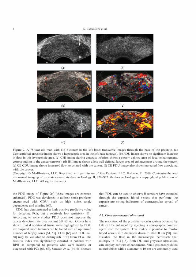
the PDU image of Figure 2(f) (these images are contrast
enhanced). PDU was developed to address some problems
encountered with CDU, such as high noise, angle
dependence and aliasing [60].
CDU has demonstrated a high positive predictive value
for detecting PCa, but a relatively low sensitivity [61].
According to some studies PDU does not improve the
cancer detection rate over sextant SB [62, 63]. Others have
shown that if additional tissue areas highlighted by PDU
are biopsied, more tumours can be found with an optimized
number of biopsy cores [64, 65]. CDU [66] and PDU [67,
68] may be valuable to distinguish BPH from PCa. The
resistive index was significantly elevated in patients with
BPH as compared to patients who were healthy or
diagnosed with PCa [66, 67]. Sauvain et al. [64, 65] showed
that PDU can be used to observe if tumours have extended
through the capsule. Blood vessels that perforate the
capsule are strong indicators of extracapsular spread of
cancer.
4.2. Contrast-enhanced ultrasound
The resolution of the prostatic vascular system obtained by
DU can be enhanced by injecting a sonographic contrast
agent into the system. This makes it possible to resolve
blood vessels with diameters down to 50–100 mm [58], and
visualize the flow in the microscopic neovessels that
multiply in PCa [18]. Both DU and greyscale ultrasound
can employ contrast enhancement. Small gas-encapsulated
microbubbles with a diameter5 10 mm are commonly used
Figure 2. A 75-year-old man with GS 8 cancer in the left base: transverse images through the base of the prostate. (a)
Conventional greyscale image shows a hypoechoic area in the left base (arrows). (b) PDU image shows no significant increase
in flow in this hypoechoic area. (c) CHI image during contrast infusion shows a clearly defined area of focal enhancement,
corresponding to the cancer (arrows). (d) IHI image shows a less well-defined, larger area of enhancement around the cancer.
(e) CE CDU image shows increased flow associated with the cancer. (f) CE PDU image also shows increased flow associated
with the cancer.
(Copyright ª MedReviews, LLC. Reprinted with permission of MedReviews, LLC. Halpern, E., 2006, Contrast-enhanced
ultrasound imaging of prostate cancer. Reviews in Urology, 8, S29–S37. Reviews in Urology is a copyrighted publication of
MedReviews, LLC. All rights reserved).
4 S. Candefjord et al.

as contrast agents [2, 58]. The lifetime of the bubbles
is5 5 min [58]. How the microbubbles react to the
ultrasound depends on its intensity [58]. At relatively low
intensities the bubbles are compressed and expanded in a
linear manner, and the bubbles then strongly reflect the
incoming wave. Nonlinear deformation of the bubbles
occurs at higher intensities, giving rise to echoes containing
higher harmonics of the incident frequency. If the acoustic
power is further increased the bubbles will eventually burst,
yielding a strong echo.
High energy ultrasound that makes the microbubbles
burst is utilized for the Doppler technique [18]. Figures 2(e)
and 2(f) show a contrast-enhanced (CE) CDU and a CE
PDU image, respectively. The latter can be compared to the
unenhanced PDU image in Figure 2(b), in which the
tumour is not visualized.
The use of contrast agents in conjunction with DU
augments the PCa detection rate significantly, as compared
to SB [18, 61]. Frauscher et al. [69, 70] performed two
prospective studies comparing the capability of 10-core SB
and CE CDU-targeted biopsies, withdrawing � 5 cores, to
detect PCa. The targeted approach detected at least as
many tumours, and more tumours of high GS, as SB. The
patient cohorts were 84 and 230 men, respectively.
Mitterberger et al. [71, 72] recently confirmed these findings
in two prospective randomized trials examining 100 and
690 men. It was shown that targeted biopsy detected
tumours of significantly higher GS as compared to SB
[71]. They also found that premedication with dutas-
teride seemed to reduce blood flow in benign prostatic
tissue [73]. This may reduce false positives e.g. from
prostatitis [73].
Greyscale ultrasound can efficiently visualize the
vascular system using contrast agents and the continuous
harmonic imaging (CHI) mode. CHI uses intermediate
ultrasound effect, which induces nonlinear microbubble
deformation, and reduces microbubble destruction as
compared to CE DU. As a result the microbubbles can
penetrate further into the microcirculation, and the
resolution of CHI is augmented as compared to DU
[18]. Higher harmonics of the fundamental frequency,
primarily originating from the microbubbles, are filtered
out. Modern technology applies broad-bandwidth ultra-
sound pulses and phase inversion, i.e. two pulses 1808out of phase are emitted, and as a consequence, the
fundamental frequency will cancel out [18]. Further
prolonged survival of the microbubbles can be achieved
by applying intermittent harmonic imaging (IHI), which
reduces the frame frequency and thus the ultrasound
effect [18]. The efficiency of CHI and IHI is demon-
strated in Figures 2(c) and 2(d), respectively.
Evaluations of the CHI and IHI techniques have shown
that they perform significantly better than sextant SB per
core, but not in total (smaller numbers of targeted biopsies
than systematic biopsies have been used) [74, 75]. Halpern
et al. [75] examined 301 patients, and cancer was found in
15.5% (175/1133) of the targeted areas versus 10.4% (188/
1806) of sextant cores (p5 0.01). The directed areas were
selected based on images from CE ultrasound using both
CHI and IHI, as well as CDU and PDU. The probability
that a core was cancerous was doubled for the targeted
cores (p5 0.001). The area under the receiver operating
characteristic curve (AUC) was at best (for IHI) 0.65. False
positives, often coupled to BPH, occur frequently when
using CE ultrasound [18]. That was also observed in a study
including 12 patients where whole-mount prostatectomy
was used as reference [76]. Several studies have excluded the
TZ to decrease this problem [70, 72].
More sensitive CE ultrasound techniques are being
developed, such as the Cadence contrast-pulse sequence
technique, which can construct images showing solely
microbubble contrast [11, 77]. Detailed information about
this technique can be found in [78]. A promising initial
study with 20 patients using targeted biopsies found that
suspicious lesions were cancerous in 8/11 cases [11]. Yang
et al. [79] used the technique to guide additional biopsies to
suspicious sites in 115 patients who underwent sextant SB.
They concluded that it was more accurate than TRUS and
PDU, and could have spared a significant number of
patients from unnecessary biopsies.
4.3. 3D ultrasound
TRUS can be extended to three dimensions by constructing
a 3D image from a series of 2D images [80]. Advanced
systems can produce real-time 3D images by means of
multiplanar ultrasound probes [7]. 3D images may be
easier to interpret than their 2D counterparts [80, 81], and
3D-TRUS can potentially reduce the inter-observer varia-
bility experienced for 2D-TRUS [80]. Only a few 3D-TRUS
studies on relatively small patient cohorts have been
conducted to date. They indicate that 3D-TRUS is not
significantly better than 2D-TRUS for detecting PCa [61,
81], but significantly improves the local staging accuracy
[80]. The 3D technique can also be applied to DU and CE
ultrasound. Hitherto few investigations have explored these
possibilities. Examining 282 men with suspected PCa
(PSA4 4 ng ml71), Sauvain et al. [64] found that 3D
PDU achieved 92.4% sensitivity and 72% specificity in
detecting PCa as compared to 87.9% and 57.6%, respec-
tively, for standard TRUS. That study showed a remark-
ably high accuracy, but the authors admit that the accuracy
was elevated due to the study design. Bogers et al. [82]
correlated 3D CE PDU and biopsy outcome in 18 patients
and showed that the sensitivity was markedly higher, 85%
as compared to 38%, than for unenhanced 3D PDU
images. Using the same technique, Sedelaar et al. [83]
detected 86% of the tumours evident at prostatectomy
specimens from 70 patients, an improvement over the 61%
reached with sextant SB.
Localization and diagnosis of prostate cancer 5
Downloaded By: [Candefjord, S.] At: 08:19 16 September 2009

4.4. Elastography
Elastography is a technique that applies ultrasound in
conjunction with external tissue compression to evaluate
the elasticity, or hardness, of tissue [84]. Hard lesions can
indicate PCa. A standard TRUS probe can be used for
imaging the prostate, and a force that compresses the gland
is applied manually by the physician via the probe [85]. The
elastogram (strain image) is generated in real time by
differentiating the spatial displacement distribution be-
tween consecutive ultrasound images [24]. Konig et al. [85]
performed a study (the first real-time elastography study to
assess PCa) in which 404 men with abnormal DRE and/or
increased PSA were examined with elastography. 151 of the
men had confirmed PCa, and elastography was able to
pinpoint 127 (84.1%) of these. Three criteria for a positive
elastography finding were applied: the lesion was marked as
being hard, the elastogram was reproducible (e.g. after
tilting of the probe), and the lesion was not suspected of
being benign in the conventional TRUS image.
Recently, in 2006–2008, a number of studies were
published that all conclude that elastography may be a
valuable tool [24, 86–90]. The performance of elastography
was rated in 15 patients using prostatectomy specimens as
reference [86]. The estimated sensitivity and specificity were
87% and 92%, respectively. A similar study succeeded in
disclosing 20 out of 27 cancers [90]. Tumours of high grade
and large volume were easier to detect. Tsutsumi et al. [89]
examined 51 men and used prostatectomy histology
correlation, reaching an overall sensitivity of 77%. Pallwein
et al. [87] conducted a prospective study including 230 men
that compared 10-core SB with targeted biopsy in the PZ,
withdrawing � 5 cores per patient. The sensitivities for
detecting PCa per patient were 72% (58/81) and 84% (68/
81) for the systematic and the elastography-directed
procedures, respectively, but the difference was not
statistically significant. However, per core the targeted
approach was significantly better (p5 0.001), and it was
almost three times more likely to prove cancer from the
lesions pointed out by elastography. All the missed
tumours, except one (1/13), were of GS � 6. Using a
similar approach the group reported 86% sensitivity and
72% specificity for the entire prostate in a study which
involved 492 men [88]. There was only moderate correla-
tion between the GS and the elastographic findings. A high
rate of false positives, 51.6%, mainly due to prostatitis, was
observed. Standard TRUS was not used to identify lesions
that might be benign.
5. Resonance sensor technology
The principle of a resonance sensor is based on the fact that
the resonance frequency of a vibrating element changes
when it is set in contact with a material. The observed
frequency shift is related to the physical hardness of the
object, and the sensor can be used to measure stiffness
variations in tissue [91]. In 1992 a resonance sensor based
on a piezoelectric element driven at its resonance frequency
by a feedback/amplifier circuit was presented by Omata &
Terunuma [92]. A piezoelectric element changes shape if
exposed to an electric field, and it will therefore oscillate in
response to a sinusoidal voltage variation. The resonance
sensor system can be made very small, as demonstrated by
Eklund et al. [93], who used a catheter tip sensor to study
the stiffness of different prostate tissue types. A miniatur-
ized instrument could potentially be used in conjunction
with ultrasound to guide biopsies [94]. Three in vitro studies
carried out by Jalkanen et al. [23, 94, 95] have shown that
the resonance sensor can distinguish cancerous tissue from
healthy glandular epithelium. However, stroma or a large
concentration of prostate stones (a benign occurrence)
could not be differentiated from cancer [23]. These authors
used a system that merges the type of resonance sensor
described by Omata and Terunuma with force and position
sensors. Lindberg et al. [96] confirmed these results
employing another resonance system that incorporates a
counter balance arrangement. The sensing volume of the
resonance sensor was recently assessed by Jalkanen et al.
[95]. It was concluded that the topical system with a
hemispherical tip laterally senses a larger area than the
actual contact area and has an estimated penetration depth
of 3.5–5.5 mm for an impression depth of 1 mm.
6. Magnetic resonance imaging (MRI)
6.1. T1- and T2-weighted MRI
MRI can depict the interior human body by analysing the
magnetic resonance (MR) signal that is generated by the
hydrogen* nuclei in the examined tissue, when the tissue is
being exposed to a strong external magnetic field and is
irradiated with a radio wave [97]. There are two main types
of signal-generating schemes used in MRI, corresponding
to the two MR relaxation times: T1-weighted (T1W) and
T2-weighted (T2W) sequences. T1W sequences cannot
depict the interior of the prostate but are useful for
observing post-biopsy haemorrhage inside the gland, as
seen in Figure 3(b) [56]. The anatomy and the internal
architecture of the gland can be clearly visualized on T2W
images, as demonstrated in Figure 3(a). Most prostate
examinations are currently carried out using a pelvic coil in
combination with an endorectal coil, at a field strength of
1.5T [98]. In the T2-mode PCa may be seen as areas with
low signal strength. However, it is hard to discern tumours
in the central gland (the TZ and the CZ are together termed
the central gland) due to the overall low intensity in
this region [99]. MRI shows a high staging accuracy for
PCa [56].
*In human tissue it is predominantly the hydrogen nucleus, abundant in
water and lipids, that yields a signal [97].
6 S. Candefjord et al.

Tumours are often confused with BPH in the central gland
[31, 56]. Furthermore, some benign features, such as
prostatitis, haemorrhage and scarring, as well as sequelae
of various therapies, can also be characterized by low
intensity [2]. Consequently, the specificity of MRI to detect
PCa is reduced to about 50% [31]. The estimated sensitivity
of MRI to detect PCa varies widely in the literature; figures
of 50–96% were demonstrated during the 1990s and 2000s
using endorectal coils and whole-mount prostatectomy
specimens as reference [31]. The discrepancies probably
arise mainly because different criteria for a positive
result have been applied, whether or not incidental (many
studies exclude tumours5 0.5 ml) and/or TZ tumours are
included, and how many segments the prostate is divided
into for the analysis [31]. Inter-observer variability is also
likely to affect the outcomes [56], and the employment of
different techniques [100]. Accordingly, studies that directly
compare SB and MRI are particularly valuable [31]. Wefer
et al. [101] compared MRI, magnetic resonance spectro-
scopic imaging (MRSI) and SB for sextant localization of
PCa in 47 patients, referring to prostatectomy histology as
reference. MRI was more sensitive, 67% (MRSI 76%)
versus 50%; but less specific, 69% (MRSI 57%) versus 82%,
than SB. Bias may have been introduced since almost half of
the patients had their biopsy performed elsewhere. In a
retrospective study including 106 men with PCa, Mullerad
et al. [102] showed that MRI added significant incremental
value to DRE and sextant SB (p5 0.0001).
A study published in 2006 [103] sheds new light on the
role of MRI in detecting TZ PCa. Two readers achieved
sensitivities of 75% and 80% and specificities of 87% and
78%, respectively, for identification of patients with
diagnosed TZ PCa by recognizing specific characteristic
imaging features of malignant lesions. That study was
retrospective and the proposed imaging features have to be
further tested [103].
6.2. Magnetic resonance spectroscopic imaging
Magnetic resonance spectroscopic imaging (MRSI) extends
the possibilities of MRI to detect PCa by allowing
assessment of molecular constituents of the tissue. The
resonance frequency of the hydrogen nucleus depends on
the chemical environment, which determines the character-
istics of the local magnetic field. For example, the frequency
of hydrogen situated in fat is shifted slightly from the
frequency of hydrogen in water. The fact that PCa has a
higher metabolism than healthy tissue is manifested in
changes in the metabolic spectra. MRSI can quantify the
metabolites citrate (Cit), choline (Cho), creatine (Cr) and
various polyamines (PA). PCa exhibits an increased
concentration of Cho and often a reduction of Cit, whereas
the level of Cr does not seem to be affected by the disease
[104]. PCa is also distinguished by lower levels of PA [105].
The peak of PA lies just between the Cho and Cr peaks in
the MRSI spectrum and therefore usually cannot be clearly
Figure 3. Gland-confined PCa. (a) Axial MRI of the prostate using an endorectal coil demonstrates a tumour (white arrow)
presenting as focal low signal in the PZ on T2W imaging (a) and intermediate signal on the T1W imaging (b). The tumour
appears as a more focal lesion than the thin, curvilinear, low signal structures representing collagen strands in the PZ
(arrowheads) on the T2W image. The periphery of the gland is well defined and the fat plane (black arrow) between the gland
and the neurovascular bundle on the left is retained, implying no capsular penetration including no neurovascular bundle
invasion.
(Reprinted from Kundra, V., 2006, Prostate cancer imaging. Seminars in Roentgenology, 41, 139–149. Copyrightª 2006, with
permission from Elsevier).
Localization and diagnosis of prostate cancer 7
Downloaded By: [Candefjord, S.] At: 08:19 16 September 2009

resolved unless state-of-the-art equipment is used [104].
However, a relatively deep dip between the Cho and Cr
peaks is indicative of PCa [105]. Figure 4 shows how MRSI
is used in conjunction with MRI to detect PCa.
The most commonly used method to detect PCa due to
changes in the metabolic spectrum is to calculate the ratioChoþCr
Cit , where the amount of each metabolite is determined
from the area of the corresponding peak [104]. The Cr peak
is included for ease of quantification because it is adjacent
to the Cho peak [106]. Jung et al. [107] suggested a
standardized interpretation system for metabolic spectra.
They used a five-point scale based on the ChoþCrCit ratio.
Adjustments were made to the initial scoring to account for
elevation of the Cho/Cr ratio and for decreased concentra-
tions of PA, and to consider poor S/N. In the study, 37 men
scheduled for radical prostatectomy were evaluated with
MRI and MRSI in the PZ. An accuracy of 74.2–85.0%
with AUC of 0.87–0.89 for the two readers was attained.
However, only clearly benign and malignant voxels were
analysed, and 15 out of 37 patients were excluded because
the spectral quality was poor. The inter-observer agreement
was excellent. Futterer et al. [108] used the standardized
interpretation system presented by Jung et al. [107], in a
prospective study using MRI and MRSI to localize PCa in
the whole prostate. The patient cohort consisted of 32 men
that would undergo radical prostatectomy. The resulting
accuracies were 81% and 87%, the AUC 0.85–0.86 and
0.86–0.91 (three readers) for the PZ and the central gland,
respectively. However, many voxel regions were assigned
unusable. Good inter-observer agreement was observed.
Wang et al. [109] performed a meta-analysis of the
literature to assess the accuracy of MRSI for PCa
detection, based on the ChoþCrCit ratio. Prospective, indepen-
dent and blind studies using prostatectomy histology, SB or
surgery as reference were included. The inclusion criteria
left only seven studies. For the diagnostic criterionChoþCr
Cit > 0:86, used as a threshold for definitive tumour,
the pooled weighted sensitivity, specificity and AUC with
corresponding 95% confidence intervals were 64% (55, 72),
86% (79, 91) and 82.7% (68.73, 96.68), respectively.
The specificity ofMRIcanbe increased substantially by the
addition ofMRSI [10, 110]. Scheidler et al. [111] reported, on
the basis of a sextant division of the prostate, a sensitivity of
95% and a specificity of 91% when MRI was used in
conjunctionwithMRSI to retrospectively detectPZPCa in53
patients. The MR findings were compared to prostatectomy
histology. The MRI detection accuracy of extracapsular
extension, as interpreted by less experienced readers, is also
significantly increased (AUC¼ 0.86 vs AUC¼ 0.75,
p5 0.05) by inclusion of MRSI [112]. The study population
was essentially the same as in Scheidler et al. [111].
MRSI may also be valuable for assessing the aggressive-
ness of PCa. It has been shown that the ChoþCrCit ratio
correlates with the GS [108, 113, 114]. Zakian et al. [114]
examined 123 patients and performed prostatectomy
histology.
Two studies recently demonstrated that new clinical
models that include MRI and MRSI data can predict the
probability of organ-confined [115] and indolent [116] PCa,
defined as small organ-confined low-grade tumours, better
than the nomograms currently in use. A recent study
showed that MRSI may potentially be used to predict the
Figure 4. Axial T2W MRI combined with MRSI of healthy
and cancerous prostate tissue. (a) The MRI was acquired
from the whole gland (heavy white box) showing a large
low signal intensity lesion (arrows) in the left PZ. (b) The
voxel from the right PZ exhibits a metabolic profile in
accordance with healthy prostatic tissue, high level of Cit
and lower concentrations of Cho and Cr. (c) The
corresponding spectrum from the left voxel shows increased
Cho and reduced Cit, indicative of PCa.
(Reprinted with kind permission from Springer ScienceþBusiness Media in Vilanova, J.C. and Barcelo, J., 2007,
Prostate cancer detection: magnetic resonance (MR)
spectroscopic imaging. Abdominal Imaging, 32, 253–261.
Figure 4. Copyright ª 2007).
8 S. Candefjord et al.

absence of PCa in men with PSA of 4–10 ng ml71 [117].
Thus, unnecessary repeated biopsies may be avoided.
6.3. Dynamic contrast-enhanced MRI
MRI can take advantage of the increased vascularity of
PCa with the help of contrast agents. Dynamic contrast-
enhanced MRI (DCE-MRI) captures T1W images of high
spatial resolution while a dose of gadolinium chelate is
injected [5,10]. Tumours can be discerned since they usually
show early signal enhancement and washout of signal
intensity, but not all tumours fit into this pattern [5].
Besides, BPH often exhibits similar enhancement curves
[31]. There is no standardized way to analyse the
enhancement curves, but many studies indicate that
tumours are best depicted 30–90 s after injection [31].
Several prospective studies using DCE-MRI in addition to
T2W sequences, correlating their findings with prostatect-
omy histology, have shown that the technique significantly
enhances the PCa detection rate using only T2W MRI [31,
118–121]. Sensitivities up to 90% were reported for
detecting PZ PCa. In addition, Hara et al. [122] demon-
strated a sensitivity of 93% and a specificity of 96% in a
patient cohort of 90 men not previously diagnosed with
PCa, but with elevated PSA level (2.55PSA5 10 ng
ml71). A 14-core SB was used as reference. Note that each
core was divided into three subcores for a total of 42
subcores, which partly accounts for the excellent specificity
[31]. A study by Vos et al. [123] indicates that it is feasible
to apply computerized analysis of prostate lesions based on
DCE-MRI. Using prostatectomy histology correlation,
they reached a PCa detection accuracy of 0.83 (AUC) in
a patient group consisting of 34 men with PZ PCa. Among
the MR techniques, DCE-MRI is in particular expected to
benefit from the use of 3T MR scanners [9, 124].
6.4. Diffusion-weighted imaging
An interesting MRI technique is diffusion-weighted ima-
ging (DWI), which can measure the diffusion of water
molecules in tissue, and hence provide information on the
structural organization of the tissue. Cancer generally
shows restricted diffusion, probably due to increased
cellular density [125]. Several recent studies, some using
3T MR systems, show that DWI used in conjunction with
T2W MRI significantly improves PCa detection as
compared to MRI alone [126–132]. Only three of the
studies [126, 127, 132] used prostatectomy histology
correlation. In the study by Morgan et al. [129], an
inexperienced reader did not obtain better results by adding
DWI to T2W MRI, raising concerns about inter-observer
disagreement. Mazaheri et al. [133] examined 38 men
scheduled for prostatectomy, and found that DWI in
combination with MRSI performed significantly better
than MRSI alone. Recent studies also show that DWI
findings may indicate tumour aggressiveness [134, 135].
DWI shows high spatial resolution and high contrast
between cancerous and healthy prostate tissue, and enables
short acquisition time [10, 136]. However, considerable
individual variations of the apparent diffusion coefficient
(ADC) have been reported [137, 138]. Another limitation is
susceptibility-induced distortions [139].
7. Vibrational spectroscopy
Raman spectroscopy (RS) and infrared (IR) spectroscopy,
jointly termed vibrational spectroscopy (VS), utilize the fact
that a molecule can start vibrating at a specific frequency in
response to light irradiation [140]. The vibrational motion
requires energy and a scattered photon undergoes a
wavelength shift that equals the frequency of the excited
vibrational mode of the particular molecule. Hence,
different molecular compositions produce unique spectra.
The biochemical information extracted by VS can reveal
the presence of cancer, which alters the molecular
composition and structure of tissue [141].
Many in vitro studies indicate that IR spectroscopy can
differentiate PCa and healthy tissue [142–147]. Gazi et al.
[148] showed that diagnostic classification (linear discrimi-
nant analysis) of Fourier transform IR spectroscopy
(FTIR) spectra correlated to the GS (5 7,¼ 7 and4 7) in
paraffin-embedded prostate tissue. A sensitivity and speci-
ficity of � 70% and � 81%, respectively, were obtained.
Furthermore, the method performed similarly to Gleason
grading in predicting metastatic tumours according to the
TNM system. This has also been shown by Malins et al.
[149]. A study conducted by Bogomolny et al. [150]
suggested that FTIR can detect malignancies early on.
Cells in culture were infected by a virus that induces
malignant transformation, and spectral changes occurred
several days earlier than visible morphological alterations.
Fernandez et al. [143] and Bhargava et al. [142] developed a
set-up capable of high throughput assessment of cells and
tissues, reaching extremely efficient classification of differ-
ent tissue types and pathologies. In vivo applications are
impeded by the very short penetration depth of IR fibre
optic probes, due to the fact that water very strongly
absorbs IR radiation [141].
The group of Crow and Stone [151–155] have evaluated
the potential of RS to detect and grade PCa in several
recent studies. They have shown that using a Raman micro
spectrometer with near-IR (832 nm) laser and linear
discriminant analysis, BPH and PCa of different biological
aggressiveness (GS5 7,¼ 7 and4 7) can be identified with
an overall accuracy of 89% [152]. The in vitro samples were
obtained from biopsies of 27 patients, 14 with BPH and 13
with PCa. Studying cultured PCa cell lines the group also
found that the stationary Raman system can almost
perfectly, with an overall sensitivity of 98% and a
specificity of 99%, differentiate between cell lines of varying
Localization and diagnosis of prostate cancer 9
Downloaded By: [Candefjord, S.] At: 08:19 16 September 2009

biological aggressiveness [154]. Taleb et al. [156] attained a
100% accurate classification of benign and malignant
(derived from metastases) prostate cells using two different
diagnostic algorithms. 30 cells were measured with a
Raman microscope set in confocal mode and equipped
with a 633 nm laser. Another study by Crow et al. [153]
measured 38 prostate samples from 37 patients and showed
that a portable fibre optic system could distinguish PCa
from BPH and prostatitis with an overall accuracy of 86%.
The group has also recently examined the biochemical basis
of different pathologies within the prostate with RS [155].
The gross biochemistry of BPH, prostatitis and three
grades of PCa (GS5 7,¼ 7 and4 7) was estimated. It was
found that the DNA content increased in cancerous tissue.
Moreover, the cholesterol level increased remarkably,
choline was elevated but remained low, triolein was
increased, whereas oleic acid decreased somewhat with
progression of disease.
8. Computer-aided detection and diagnosis
Many studies have shown that computerized interpretation
of data can improve the accuracy of PCa detection and
prediction of the pathologic stage [20]. Artificial neural
networks and support vectormachines are powerful tools for
handling complex and possibly nonlinear relationships
between variables, and these are promising for improving
the accuracy of nomograms. High accuracies have been
demonstrated in some studies, but the full potential has not
been elucidated yet [20]. Computerizedmethods for identify-
ing cancerous tissue in images obtained by ultrasound and
MRI are being investigated intensively [11, 20, 123, 157–161].
For example, Mohamed et al. [57] reached an accuracy of
93.75% for automatic detection of PCa in greyscale
ultrasound images. They used an algorithm that segments
the ultrasound image into regions of interest, ranks
different texture features, and selects the most important
ones. Bertaccini et al. [157] performed a blind prospective
study on 105 patients with suspected PCa using preproces-
sing of greyscale ultrasound data, and showed that 26/32
tumours evident at biopsy could be detected. Computer-
assisted detection using CE ultrasound is being developed,
and could be based on contrast enhancement as a function
of time, since contrast agents typically flow faster through
malignant than benign areas [11]. Objective image inter-
pretation may reduce inter-observer variation [20].
9. Discussion
Table 1 provides an overview and comparison of the
methods included in this review. The advantages and
disadvantages of each technique, and concluding remarks,
are given. This discussion section is based on Table 1.
CE ultrasound has been shown to outperform today’s
gold standard by detecting more clinically significant
tumours with fewer cores [11, 162, 163]. However, the
image reading is subjective and the inter-observer agree-
ment is not satisfactory [11, 18, 75]. Work is ongoing to
develop computer-assisted detection for CE techniques [11,
164]. Contrast agents bring high costs per core, but CE
techniques may be cost-effective due to a reduction of the
number of cores [69]. Frequent false-positive findings have
been reported. Premedication that reduces blood flow in
benign lesions can potentially reduce the number of false
positives [73]. A report on a multicentre European
coordination project [77] provides good evidence of the
safety of CE ultrasound. Unfortunately, the project did not
achieve its goal of initiating a multicentre study that could
prove an additional clinical value of CE ultrasound.
However, the authors state that such a study will be
initiated.
Elastography is a promising new method that may
improve PCa detection. It is not yet feasible, due to
technical limitations, to implement an absolute tissue
hardness threshold that indicates cancer and enables
objective interpretation [88]. No data have been presented
that evaluate intra- and inter-observer variability. The main
limitation of elastography seems to be that benign lesions,
primarily prostatitis and BPH, can be hard to distinguish
from tumours [86, 88].
As can be deducted from Table 1 the new MR techniques
are very promising. They show good potential for highly
accurate detection, and for excluding disease and decreas-
ing the need for repeated biopsy. The performance of T2W
MRI is not sufficiently accurate for its use to be advised in
screening [2, 31, 61]. MRSI in conjunction with MRI has
shown high accuracies for detecting PCa in many studies,
and the combination holds promise for non-invasively
grading tumours and predicting indolent disease. New
metabolic biomarkers may further improve the grading
accuracy of MRSI [165, 166]. Furthermore, interpretation
of the metabolic profile can be standardized and computer-
ized to eliminate inter-observer disagreement. Drawbacks
of MRSI are the long acquisition time, the high frequency
of spectral artefacts and low spatial resolution at 1.5T [10,
136, 167]. The addition of DCE-MRI to T2W sequences
significantly improves the detection rate [31]. DCE-MRI
shows limitations in differentiating PCa from prostatitis
and BPH [139]. There are concerns about the safety
of gadolinium-based contrast agents [168]. Moreover,
DCE-MRI has difficulties discerning TZ tumours [136].
DWI shows good potential for improving MRI detection,
but more studies are needed to assess its accuracy [10, 167].
Individual variations of the ADC may impair diagnostic
performance [136]. The diagnostic performance of MR
techniques may be further improved at 3T [9].
A combination of several MR techniques (MRI, MRSI,
DCE-MRI and DWI) is likely to detect PCa most
efficiently. According to Kirkham et al. [31] it is reasonable
to hope that multiparametric MRI will detect about 90% of
10 S. Candefjord et al.
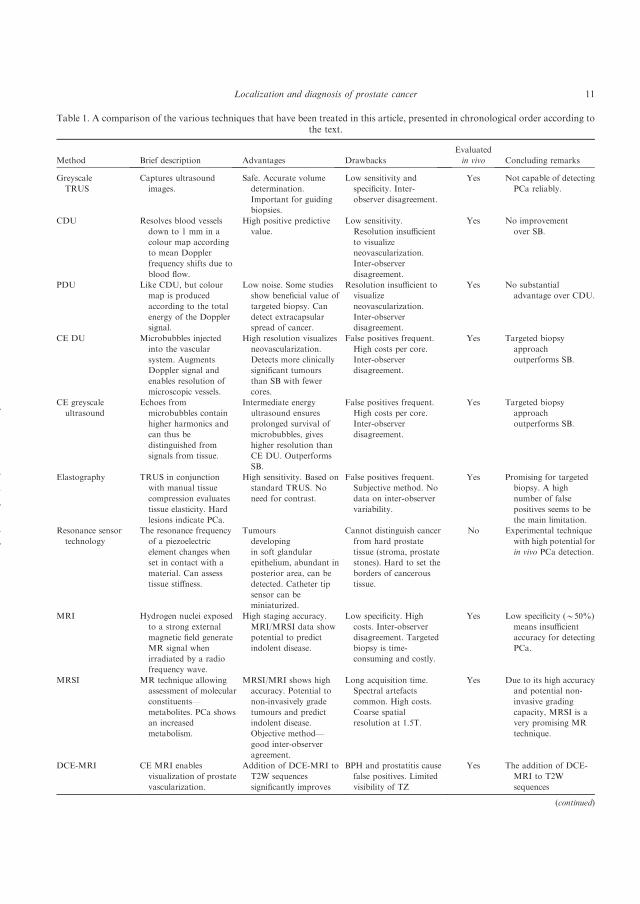
Table 1. A comparison of the various techniques that have been treated in this article, presented in chronological order according tothe text.
Method Brief description Advantages Drawbacks
Evaluated
in vivo Concluding remarks
Greyscale
TRUS
Captures ultrasound
images.
Safe. Accurate volume
determination.
Important for guiding
biopsies.
Low sensitivity and
specificity. Inter-
observer disagreement.
Yes Not capable of detecting
PCa reliably.
CDU Resolves blood vessels
down to 1 mm in a
colour map according
to mean Doppler
frequency shifts due to
blood flow.
High positive predictive
value.
Low sensitivity.
Resolution insufficient
to visualize
neovascularization.
Inter-observer
disagreement.
Yes No improvement
over SB.
PDU Like CDU, but colour
map is produced
according to the total
energy of the Doppler
signal.
Low noise. Some studies
show beneficial value of
targeted biopsy. Can
detect extracapsular
spread of cancer.
Resolution insufficient to
visualize
neovascularization.
Inter-observer
disagreement.
Yes No substantial
advantage over CDU.
CE DU Microbubbles injected
into the vascular
system. Augments
Doppler signal and
enables resolution of
microscopic vessels.
High resolution visualizes
neovascularization.
Detects more clinically
significant tumours
than SB with fewer
cores.
False positives frequent.
High costs per core.
Inter-observer
disagreement.
Yes Targeted biopsy
approach
outperforms SB.
CE greyscale
ultrasound
Echoes from
microbubbles contain
higher harmonics and
can thus be
distinguished from
signals from tissue.
Intermediate energy
ultrasound ensures
prolonged survival of
microbubbles, gives
higher resolution than
CE DU. Outperforms
SB.
False positives frequent.
High costs per core.
Inter-observer
disagreement.
Yes Targeted biopsy
approach
outperforms SB.
Elastography TRUS in conjunction
with manual tissue
compression evaluates
tissue elasticity. Hard
lesions indicate PCa.
High sensitivity. Based on
standard TRUS. No
need for contrast.
False positives frequent.
Subjective method. No
data on inter-observer
variability.
Yes Promising for targeted
biopsy. A high
number of false
positives seems to be
the main limitation.
Resonance sensor
technology
The resonance frequency
of a piezoelectric
element changes when
set in contact with a
material. Can assess
tissue stiffness.
Tumours
developing
in soft glandular
epithelium, abundant in
posterior area, can be
detected. Catheter tip
sensor can be
miniaturized.
Cannot distinguish cancer
from hard prostate
tissue (stroma, prostate
stones). Hard to set the
borders of cancerous
tissue.
No Experimental technique
with high potential for
in vivo PCa detection.
MRI Hydrogen nuclei exposed
to a strong external
magnetic field generate
MR signal when
irradiated by a radio
frequency wave.
High staging accuracy.
MRI/MRSI data show
potential to predict
indolent disease.
Low specificity. High
costs. Inter-observer
disagreement. Targeted
biopsy is time-
consuming and costly.
Yes Low specificity (*50%)
means insufficient
accuracy for detecting
PCa.
MRSI MR technique allowing
assessment of molecular
constituents—
metabolites. PCa shows
an increased
metabolism.
MRSI/MRI shows high
accuracy. Potential to
non-invasively grade
tumours and predict
indolent disease.
Objective method—
good inter-observer
agreement.
Long acquisition time.
Spectral artefacts
common. High costs.
Coarse spatial
resolution at 1.5T.
Yes Due to its high accuracy
and potential non-
invasive grading
capacity, MRSI is a
very promising MR
technique.
DCE-MRI CE MRI enables
visualization of prostate
vascularization.
Addition of DCE-MRI to
T2W sequences
significantly improves
BPH and prostatitis cause
false positives. Limited
visibility of TZ
Yes The addition of DCE-
MRI to T2W
sequences
(continued)
Localization and diagnosis of prostate cancer 11
Downloaded By: [Candefjord, S.] At: 08:19 16 September 2009

significant cancers. Early studies show promising results
[169–171]. However, it remains to be solved how such large
amounts of data should be optimally analysed [10].
Although MRI could be used for guiding biopsies, the
procedure is more complex and time-consuming than
TRUS, and the clinical practicability is questionable [31,
172, 173]. Presently, there is a lack of accuracy of fusing
MRI and TRUS images; better methods are needed to
utilize MR data in TRUS-directed biopsy [167, 174]. In the
future MR-guided biopsy may be performed via robotic
systems, and preliminary studies have shown that accurate
needle placement is feasible [173, 175]. High costs and
limited availability of MR scanners at present impedes the
feasibility of MRI [139].
Experimental techniques, which are summarized in Table
1, such as resonance sensor technology and RS, are also
interesting. These methods have so far only been evaluated
in vitro. The resonance sensor has potential for non-
invasively detecting PCa, but the diagnostic accuracy must
be improved. Spectroscopic techniques are promising for
objective PCa detection and diagnosis. RS has shown an
excellent capability to distinguish between cancerous and
healthy tissue as well as grading PCa. However, RS cannot
detect PCa non-invasively due to a shallow penetration
depth [176]. Development of techniques that can sense
deeper into the tissue, such as time-gated RS [176] and
spatially offset probes [177], is ongoing. Minimally invasive
examinations of the prostate are possible since Raman fibre
optic probes thinner than the diameter of common clinical
devices such as needles and endoscopes, typically 1–2 mm
thick [178], have been demonstrated [179]. Spectroscopic
techniques have great potential for aiding histopathologic
examinations [180], which are subjective and time-consum-
ing. A questionnaire indicates that the long waiting time for
biopsy results causes the most anxiety in patients under-
going screening for PCa [181]. Novel techniques for PCa
detection are needed, since both ultrasound and MR
techniques show many limitations [182].
Computer-aided detection and diagnosis is likely to play
an important role in the future. Intra- and inter-observer
variability is a problem with both ultrasound and MR
technology. Morphologic and/or functional images are
hard to interpret. The high and increasing clinical incidence
of PCa presents the urologist with an ever increasing
amount of data to analyse. Computer-aided detection and
diagnosis have the potential to evaluate complex data
objectively, consistently, and in a time- and cost-efficient
manner.
To distinguish between indolent and aggressive tumours
is of utmost importance for improving patient care. There
is a range of treatment options available today, and
minimally invasive therapies are gaining interest among
patients since radical prostatectomy is associated with
potential morbidity [183, 184]. More precise disease
Table 1. (Continued).
Method Brief description Advantages Drawbacks
Evaluated
in vivo Concluding remarks
detection. Fast. High
spatial resolution.
tumours. High costs.
Are gadolinium-based
contrast agents safe?
significantly improves
detection accuracy.
DWI MR technique that can
measure the ADC of
tissue. PCa shows
reduced diffusion.
Initial studies indicate
significantly higher
detection rate using
DWIþT2W MRI.
Fast. High contrast
between cancerous and
healthy tissue. High
spatial resolution.
Variation of the ADC
between different
individuals.
Susceptibility-induced
distortions. High costs.
Yes DWI seems to improve
MRI detection
accuracy.
RS Monochromatic light
changes polarizability
of molecules, which
start to vibrate—
inelastic scattering of
light induces
wavelength shift.
In vitro studies show very
high accuracy. Can
objectively distinguish
different grades of
malignancy.
Low penetration depth of
current fibre optic
probes excludes
non-invasive detection.
Laser light might affect
tissue.
No Experimental technique
with high detection
and grading
accuracies.
IR spectroscopy Measures absorption of
polychromatic IR
radiation, which
changes the dipole
moment of the
interacting molecules.
In vitro trials demonstrate
potential to objectively
detect and grade PCa.
Some studies indicate
similar predictive
capacities as the GS.
Difficult to examine tissue
with fibre optic probes.
No Experimental technique
with potential to
detect and grade PCa.
In vivo measurements
difficult.
12 S. Candefjord et al.
characterization is a major objective of PCa imaging [8].
CE ultrasound and elastography data show correlation
with the GS. However, in our opinion MR techniques are
more promising for grading cancer, since MRSI enables
assessment of the chemical contents of the tissue.
A large number of studies on PCa detection and
diagnosis are published every year. However, only a few
studies follow a rigid study protocol, and the majority of
publications contribute little to assessing the clinical value
of the methods. This was stressed in the meta-analysis of
MRSI reports performed by Wang et al. [109], where only
seven MRSI studies met the inclusion criteria, and merely
two studies qualified as grade A according to the criteria of
diagnostic research published by the Cochrane centre.
Long-term follow-up of the clinical significance of the
detected tumours is rarely carried out [18]. The hetero-
geneity of the design and outcome of different studies blurs
the picture of whether new ultrasound and MR methods
add significant clinical value. The discrepancy of the
reported sensitivity of T2W MRI, reviewed in x6.1, is a
clear example. Studies that correlate the imaging findings
with SB do not estimate the sensitivity reliably [109].
Comparisons between SB and targeted biopsy are valuable,
however, and relatively many studies using ultrasound
techniques have been published. The first studies using
MR-guided biopsy, which has not been feasible before, are
now being published.
To obtain a clear picture of the clinical usefulness of
different techniques large-scale multi-centre studies of high
quality are necessary [77, 109]. The lack of such publica-
tions may be explained by several factors including
limitations of funding, intellectual property rights, sharing
of data, refinement of the technique during the study
period, and parochial interests such as individual career
advancement [185]. To gain clinical acceptance of new
methods they must be standardized, and clinical benefits
and cost-effectiveness must be clearly shown. There are
several ultrasound and MR techniques that have the
potential to increase the clinical detection rate and
diagnostic accuracy for PCa.
10. Conclusion
The current gold standard of PCa detection, SB, has limited
sensitivity and difficulties evaluating tumour aggressive-
ness. PSA screening leads to over-treatment of many men
and its value for reducing PCa mortality is controversial.
To detect and grade PCa early on remains challenging.
Recent developments of ultrasound techniques indicate
that it is possible to disclose more clinically significant
cancers with a reduced number of cores by means of
targeted biopsy approaches. Advances of MR techniques
significantly improve the detection accuracy of MRI, and
multiparametric MRI is very promising. Inter-observer
disagreement is an issue with both conventional MRI and
ultrasound. MRSI is the first method to offer an objective
way of assessing PCa, but computer-aided detection based
on CE and standard ultrasound and MR techniques is
emerging as well. Limited availability of MR scanners, the
questionable practicability of MR-directed biopsy and high
costs limit the usefulness of MR methods at present. There
are also alternative experimental techniques, resonance
sensor technology and VS that have shown promising
results in vitro. Appropriate tools for updating the gold
standard are available, but large-scale prospective multi-
centre studies are needed to determine the clinical benefits
of these new methods.
Acknowledgements
The study was funded by the Objective 2 Norra Norrland—
EU Structural Fund.
References
[1] Ferlay, J., Autier, P., Boniol, M., Heanue, M., Colombet, M. and
Boyle, P., 2007, Estimates of the cancer incidence and mortality in
Europe in 2006. Annals of Oncology, 18, 581–592.
[2] Fitzsimons, N.J., Sun, L. and Moul, J.W., 2007, Medical techno-
logies for the diagnosis of prostate cancer. Expert Review of Medical
Devices, 4, 227–239.
[3] Sim, H.G. and Cheng, C.W.S., 2005, Changing demography of
prostate cancer in Asia. European Journal of Cancer, 41, 834–845.
[4] Olsson, C., 1993, Prostatic cancer. Kidney International, 43, 955–965.
[5] Hricak, H., Choyke, P.L., Eberhardt, S.C., Leibel, S.A. and
Scardino, P.T., 2007, Imaging prostate cancer: A multidisciplinary
perspective. Radiology, 243, 28–53.
[6] Kundra, V., 2006, Prostate cancer imaging. Seminars in Roentgeno-
logy, 41, 139–149.
[7] Loch, T., 2007, Urologic imaging for localized prostate cancer in
2007. World Journal of Urology, 25, 121–129.
[8] Fuchsjager, M., Shukla-Dave, A., Akin, O., Barentsz, J. and Hricak,
H., 2008, Prostate cancer imaging. Acta Radiology, 49, 107–120.
[9] Kim, C.K. and Park, B.K., 2008, Update of prostate magnetic
resonance imaging at 3T. Journal of Computer Assisted Tomography,
32, 163–172.
[10] Kurhanewicz, J., Vigneron, D., Carroll, P. and Coakley, F., 2008,
Multiparametric magnetic resonance imaging in prostate cancer:
present and future. Current Opinions in Urology, 18, 71–77.
[11] Pallwein, L., Mitterberger, M., Pelzer, A., Bartsch, G., Strasser, H.,
Pinggera, G.M., Aigner, F., Gradl, J., Nedden, D.Z. and Frauscher,
F., 2008, Ultrasound of prostate cancer: recent advances. European
Radiology, 18, 707–715.
[12] Costello, L.C. and Franklin, R.B., 2009, Prostatic fluid electrolyte
composition for the screening of prostate cancer: a potential solution to
a major problem. Prostate Cancer and Prostatic Diseases, 12, 17–24.
[13] De Angelis, G., Rittenhouse, H.G., Mikolajczyk, S.D., Blair Shamel,
L., and Semjonow, A., 2007, Twenty years of PSA: from prostate
antigen to tumor marker. Reviews in Urology, 9, 113–123.
[14] McNeal, J.E., Redwine, E.A., Freiha, F.S. and Stamey, T.A., 1988,
Zonal distribution of prostatic adenocarcinoma. Correlation with
histologic pattern and direction of spread. American Journal of
Surgical Pathology, 12, 897–906.
[15] Boczko, J., Messing, E. and Dogra, V., 2006, Transrectal sonography
in prostate evaluation. Radiologic Clinics of North America, 44, 679–
687.
Localization and diagnosis of prostate cancer 13
Downloaded By: [Candefjord, S.] At: 08:19 16 September 2009

[16] Gjengstø, P.,Halvorsen,O.J., Akslen, L.A., Frugard, J. andHoisaeter,
P.A., 2003, Benign growth of different prostate zones in agingmenwith
slightly elevated PSA in whom prostate cancer has been excluded: a
prospective study of 510 patients. Urology, 62, 447–450.
[17] Tang, J., Yang, J.C., Zhang, Y., Liu, X., Zhang, L., Wang, Z., Li, J.,
Luo, Y., Xu, J. and Shi, H., 2007, Does benign prostatic hyperplasia
originate from the peripheral zone of the prostate? A preliminary
study. BJU International, 100, 1091–1096.
[18] Halpern, E.J., 2006, Contrast-enhanced ultrasound imaging of
prostate cancer. Reviews in Urology, 8 Suppl 1, S29–S37.
[19] Neal, D.E., Leung, H.Y., Powell, P.H., Hamdy, F.C. and Donovan,
J.L., 2000, Unanswered questions in screening for prostate cancer.
European Journal of Cancer, 36, 1316–1321.
[20] Zhu, Y., Williams, S. and Zwiggelaar, R., 2006, Computer
technology in detection and staging of prostate carcinoma: a review.
Medical Image Analysis, 10, 178–199.
[21] Bergh, A., Gronberg, H., Hedestig, O., Stattin, P., Widmark, A. and
Wikstrom, P., 2005, Prostatacancer—Mannens Gissel. (Umea:
Faculty of Medicine at Umea University).
[22] Raja, J., Ramachandran, N., Munneke, G. and Patel, U., 2006,
Current status of transrectal ultrasound guided prostate biopsy in the
diagnosis of prostate cancer. Clinical Radiology, 61, 142–153.
[23] Jalkanen, V., Andersson, B.M., Bergh, A., Ljungberg, B. and
Lindahl, O.A., 2006, Resonance sensor measurements of stiffness
variations in prostate tissue in vitro—a weighted tissue proportion
model. Physiological Measurement, 27, 1373–1386.
[24] Miyanaga, N., Akaza, H., Yamakawa, M., Oikawa, T., Sekido, N.,
Hinotsu, S., Kawai, K., Shimazui, T. and Shiina, T., 2006, Tissue
elasticity imaging for diagnosis of prostate cancer: a preliminary
report. International Journal of Urology, 13, 1514–1518.
[25] Zhang, M., Nigwekar, P., Castaneda, B., Hoyt, K., Joseph, J.V., di
Sant’Agnese, A., Messing, E.M., Strang, J.G., Rubens, D.J. and
Parker, K.J., 2008, Quantitative characterization of viscoelastic
properties of human prostate correlated with histology. Ultrasound
in Medicine and Biology, 34, 1033–1042.
[26] Heidenreich, A., Aus, G., Bolla, M., Joniau, S., Matveev, V.B.,
Schmid, H.P. and Zattoni, F., 2008, EAU guidelines on prostate
cancer. European Urology, 53, 68–80.
[27] Hodge, K.K., McNeal, J.E., Terris, M.K. and Stamey, T.A., 1989,
Random systematic versus directed ultrasound guided transrectal
core biopsies of the prostate. Journal of Urology, 142, 71–74;
discussion 74–75.
[28] Rabbani, F., Stroumbakis, N., Kava, B.R., Cookson, M.S. and Fair,
W.R., 1998, Incidence and clinical significance of false-negative
sextant prostate biopsies. Journal of Urology, 159, 1247–1250.
[29] Jones, J.S., Patel, A., Schoenfield, L., Rabets, J.C., Zippe, C.D. and
Magi-Galluzzi, C., 2006, Saturation technique does not improve
cancer detection as an initial prostate biopsy strategy. Journal of
Urology, 175, 485–488.
[30] Lane, B.R., Zippe, C.D., Abouassaly, R., Schoenfield, L., Magi-
Galluzzi, C. and Jones, J.S., 2008, Saturation technique does not
decrease cancer detection during follow up after initial prostate
biopsy. Journal of Urology, 79, 1746–1750.
[31] Kirkham, A.P.S., Emberton, M. and Allen, C., 2006, How good is
MRI at detecting and characterising cancer within the prostate?
European Urology, 50, 1163–1174; discussion 1175.
[32] Catalona, W.J., Loeb, S. and Han, M., 2006, Viewpoint: expanding
prostate cancer screening. Annals of Internal Medicine, 144, 441–443.
[33] Helzlsouer, K.J., Newby, J. and Comstock, G.W., 2008, Prostate-
specific antigen levels and subsequent prostate cancer: potential for
screening. American Journal Of Epidemiology, 168, 841–844 (rep-
rinted from Cancer Epidemiology, Biomarkers & Prevention, 1992, 1,
537–540).
[34] USPSTF, 2008, Screening for prostate cancer: US Preventive Services
Task Force recommendation statement. Annals of Internal Medicine,
149, 185–191.
[35] Ahyai, S.A., Graefen, M., Steuber, T., Haese, A., Schlomm, T.,
Walz, J., Kollermann, J., Briganti, A., Zacharias, M., Friedrich,
M.G., Karakiewicz, P.I., Montorsi, F., Huland, H. and Chun,
F.K.-H., 2008, Contemporary prostate cancer prevalence among T1c
biopsy-referred men with a prostate-specific antigen level5 or¼ 4.0
ng per milliliter. European Urology, 53, 750–757.
[36] Thompson, I.M., Pauler, D.K., Goodman, P.J., Tangen, C.M.,
Lucia, M.S., Parnes, H.L., Minasian, L.M., Ford, L.G., Lippman,
S.M., Crawford, E.D., Crowley, J.J., and Coltman, C.A., 2004,
Prevalence of prostate cancer among men with a prostate-specific
antigen level5 or¼ 4.0 ng per milliliter. New England Journal of
Medicine, 350, 2239–2246.
[37] Montironi, R., Mazzuccheli, R., Scarpelli, M., Lopez-Beltran, A.,
Fellegara, G., and Algaba, F., 2005, Gleason grading of prostate
cancer in needle biopsies or radical prostatectomy specimens:
contemporary approach, current clinical significance and sources of
pathology discrepancies. BJU International, 95, 1146–1152.
[38] Coard, K.C. and Freeman, V.L., 2004, Gleason grading of prostate
cancer: level of concordance between pathologists at the University
Hospital of the West Indies. American Journal of Clinical Pathology,
122, 373–376.
[39] Fukagai, T., Namiki, T., Namiki, H., Carlile, R.G., Shimada, M. and
Yoshida, H., 2001, Discrepancies between Gleason scores of needle
biopsy and radical prostatectomy specimens. Pathology International,
51, 364–370.
[40] Maygarden, S.J. and Pruthi, R., 2005, Gleason grading and volume
estimation in prostate needle biopsy specimens: evolving issues.
American Journal of Clinical Pathology, 123 Suppl, S58–S66.
[41] Ooi, K. and Samali, R., 2007, Discrepancies in Gleason scoring of
prostate biopsies and radical prostatectomy specimens and the effects
of multiple needle biopsies on scoring accuracy.A regional experience
in Tamworth, Australia. ANZ Journal of Surgery, 77, 336–338.
[42] Tomioka, S., Nakatsu, H., Suzuki, N., Murakami, S., Matsuzaki, O.
and Shimazaki, J., 2006, Comparison of Gleason grade and score
between preoperative biopsy and prostatectomy specimens in
prostate cancer. International Journal of Urology, 13, 555–559.
[43] Aihara, M., Wheeler, T.M., Ohori, M. and Scardino, P.T., 1994,
Heterogeneity of prostate cancer in radical prostatectomy specimens.
Urology, 43, 60–66; discussion 66–67.
[44] Sooriakumaran, P., Lovell, D.P., Henderson, A., Denham, P.,
Langley, S.E.M. and Laing, R.W., 2005, Gleason scoring varies
among pathologists and this affects clinical risk in patients with
prostate cancer. Clinical Oncology, 17, 655–658.
[45] Dall’Era, M.A., Konety, B.R., Cowan, J.E., Shinohara, K., Stauf, F.,
Cooperberg, M.R., Meng, M.V., Kane, C.J., Perez, N., Master, V.A.
and Carroll, P.R., 2008, Active surveillance for the management
of prostate cancer in a contemporary cohort. Cancer, 112, 2664–
2670.
[46] Yin, M., Bastacky, S., Chandran, U., Becich, M.J. and Dhir, R.,
2008, Prevalence of incidental prostate cancer in the general
population: a study of healthy organ donors. Journal of Urology,
179, 892–895; discussion 895.
[47] Watanabe, H., Kaiho, H., Tanaka, M. and Terasawa, Y., 1971,
Diagnostic application of ultrasonotomography to the prostate.
Investigative Urology, 8, 548–559.
[48] Watanabe, H., Igari, D., Tanahashi, Y., Harada, K. and Saito, M.,
1974, Measurements of size and weight of prostate by means of
transrectal ultrasonotomography. Tohoku Journal of Experimental
Medicine, 114, 277–285.
[49] Watanabe, H., Igari, D., Tanahashi, Y., Harada, K., and Saitoh, M.,
1975, Transrectal ultrasonotomography of the prostate. Journal of
Urology, 114, 734–739.
[50] Watanabe, H., Igari, D., Tanahashi, Y., Harada, K. and Saitoh, M.,
1976, An evaluation of the function of new special equipment for
transrectal ultrasonotomography. Tohoku Journal of Experimental
Medicine, 118, 387–392.
14 S. Candefjord et al.

[51] Toi, A., Neill, M.G., Lockwood, G.A., Sweet, J.M., Tammsalu, L.A.
and Fleshner, N.E., 2007, The continuing importance of transrectal
ultrasound identification of prostatic lesions. Journal of Urology, 177,
516–520.
[52] Oyen, R.H., Van de Voorde, W.M., Van Poppel, H.P., Brys, P.P.,
Ameye, F.E., Franssens, Y.M., Baert, A.L. and Baert, L.V., 1993,
Benign hyperplastic nodules that originate in the peripheral zone of
the prostate gland. Radiology, 189, 707–711.
[53] Lee, F., Torp-Pedersen, S., Littrup, P.J., McLeary, R.D., McHugh,
T.A., Smid, A.P., Stella, P.J. and Borlaza, G.S., 1989, Hypoechoic
lesions of the prostate: clinical relevance of tumor size, digital rectal
examination, and prostate-specific antigen. Radiology, 170, 29–32.
[54] Carter,H.B.,Hamper,U.M., Sheth, S., Sanders,R.C., Epstein, J.I. and
Walsh, P.C., 1989, Evaluation of transrectal ultrasound in the early
detection of prostate cancer. Journal of Urology, 142, 1008–1010.
[55] Flanigan, R.C., Catalona, W.J., Richie, J.P., Ahmann, F.R.,
Hudson, M.A., Scardino, P.T., deKernion, J.B., Ratliff, T.L.,
Kavoussi, L.R. and Dalkin, B.L., 1994, Accuracy of digital rectal
examination and transrectal ultrasonography in localizing prostate
cancer. Journal of Urology, 152, 1506–1509.
[56] Carey, B.M., 2005, Imaging for prostate cancer. Clinical Oncology,
17, 553–559.
[57] Mohamed, S.S., Salama, M.M.A., Kamel, M., El-Saadany, E.F.,
Rizkalla, K. and Chin, J., 2005, Prostate cancer multi-feature
analysis using trans-rectal ultrasound images. Physics in Medicine
and Biology, 50, N175–N185.
[58] Padhani, A.R., Harvey, C.J. and Cosgrove, D.O., 2005, Angiogenesis
imaging in the management of prostate cancer. Nature Clinical
Practice Urology, 2, 596–607.
[59] Bude, R.O. and Rubin, J.M., 1996, Power Doppler sonography.
Radiology, 200, 21–23.
[60] Rubin, J.M., Bude, R.O., Carson, P.L., Bree, R.L. and Adler, R.S.,
1994, Power Doppler US: a potentially useful alternative to mean
frequency-based color Doppler US. Radiology, 190, 853–856.
[61] Amiel, G.E. and Slawin, K.M., 2006, Newer modalities of ultrasound
imaging and treatment of the prostate. Urologic Clinics of North
America, 33, 329–337.
[62] Arger, P.H., Malkowicz, S.B., Van Arsdalen, K.N., Sehgal, C.M.,
Holzer, A. and Schultz, S.M., 2004, Color and power Doppler
sonography in the diagnosis of prostate cancer: comparison between
vascular density and total vascularity. Journal of Ultrasound
Medicine, 23, 623–630.
[63] Halpern, E.J. and Strup, S.E., 2000, Using gray-scale and color and
power Doppler sonography to detect prostatic cancer. American
Journal of Roentgenology, 174, 623–627.
[64] Sauvain, J.L., Palascak, P., Bourscheid, D., Chabi, C., Atassi, A.,
Bremon, J.M. and Palascak, R., 2003, Value of power doppler and
3D vascular sonography as a method for diagnosis and staging of
prostate cancer. European Urology, 44, 21–30; discussion 30–1.
[65] Sauvain, J.L., Palascak, P., Nader, N., Gomez, W., Bloqueau, Ph.,
Bremon, J.M., Jung, L., Maniere, Ph. and Papavero, R., 2006, Power
Doppler Imaging and prostate cancer: optional or necessary
technique? Journal of Radiology, 87, 1063–1072.
[66] Berger, A.P., Horninger, W., Bektic, J., Pelzer, A., Spranger, R.,
Bartsch, G. and Frauscher, F., 2006, Vascular resistance in the
prostate evaluated by colour Doppler ultrasonography: is benign
prostatic hyperplasia a vascular disease? BJU International, 98, 587–
590.
[67] Kojima, M., Ochiai, A., Naya, Y., Okihara, K., Ukimura, O. and
Miki, T., 2000, Doppler resistive index in benign prostatic
hyperplasia: correlation with ultrasonic appearance of the prostate
and infravesical obstruction. European Urology, 37, 436–442.
[68] Turgut, A.T., Olucuoglu, E., Kosar, P., Geyik, P.O., Kosar, U. and
Dogra, V., 2007, Power Doppler ultrasonography of the feeding
arteries of the prostate gland: a novel approach to the diagnosis of
prostate cancer? Journal of Ultrasound Medicine, 26, 875–883.
[69] Frauscher, F., Klauser, A., Halpern, E.J., Horninger, W. and
Bartsch, G., 2001, Detection of prostate cancer with a microbubble
ultrasound contrast agent. Lancet, 357, 1849–1850.
[70] Frauscher, F., Klauser, A., Volgger, H., Halpern, E.J., Pallwein, L.,
Steiner, H., Schuster, A., Horninger, W., Rogatsch, H. and Bartsch,
G., 2002, Comparison of contrast enhanced color Doppler targeted
biopsy with conventional systematic biopsy: impact on prostate
cancer detection. Journal of Urology, 167, 1648–1652.
[71] Mitterberger, M., Pinggera, G.M., Horninger, W., Bartsch, G.,
Strasser, H., Schafer, G., Brunner, A., Halpern, E.J., Gradl, J.,
Pallwein, L. and Frauscher, F., 2007, Comparison of contrast
enhanced color Doppler targeted biopsy to conventional systematic
biopsy: impact on Gleason score. Journal of Urology, 178, 464–468;
discussion 468.
[72] Mitterberger, M., Horninger, W., Pelzer, A., Strasser, H., Bartsch, G.,
Moser, P., Halpern, E.J., Gradl, J., Aigner, F., Pallwein, L. and
Frauscher, F., 2007, A prospective randomized trial comparing
contrast-enhanced targeted versus systematic ultrasound guided
biopsies: impact on prostate cancer detection.Prostate, 67, 1537–1542.
[73] Mitterberger, M., Pinggera, G., Horninger, W., Strasser, H.,
Halpern, E., Pallwein, L., Gradl, J., Bartsch, G. and Frauscher, F.,
2008, Dutasteride prior to contrast-enhanced colour Doppler
ultrasound prostate biopsy increases prostate cancer detection.
European Urology, 53, 112–117.
[74] Halpern, E.J., Frauscher, F., Rosenberg, M. and Gomella, L.G.,
2002, Directed biopsy during contrast-enhanced sonography of the
prostate. American Journal of Roentgenology, 178, 915–919.
[75] Halpern, E.J., Ramey, J.R., Strup, S.E., Frauscher, F., McCue, P.
and Gomella, L.G., 2005, Detection of prostate carcinoma with
contrast-enhanced sonography using intermittent harmonic imaging.
Cancer, 104, 2373–2383.
[76] Halpern, E.J., McCue, P.A., Aksnes, A.K., Hagen, E.K., Frauscher,
F. and Gomella, L.G., 2002, Contrast-enhanced US of the prostate
with Sonazoid: comparison with whole-mount prostatectomy speci-
mens in 12 patients. Radiology, 222, 361–366.
[77] Wink, M., Frauscher, F., Cosgrove, D., Chapelon, J.-Y., Palwein, L.,
Mitterberger, M., Harvey, C., Rouviere, O., de la Rosette, J. and
Wijkstra, H., 2008, Contrast-enhanced ultrasound and prostate
cancer; a multicentre European research coordination project.
European Urology, 54, 982–993.
[78] Phillips, P. and Gardner, E., 2004, Contrast-agent detection and
quantification. European Radiology, 14 Suppl 8, P4–10.
[79] Yang, J.C., Tang, J., Li, J., Luo, Y., Li, Y. and Shi, H., 2008,
Contrast-enhanced gray-scale transrectal ultrasound-guided prostate
biopsy in men with elevated serum prostate-specific antigen levels.
Academic Radiology, 15, 1291–1297.
[80] Mehta, S.S., Azzouzi, A.R. and Hamdy, F.C., 2004, Three
dimensional ultrasound and prostate cancer. World Journal of
Urology, 22, 339–345.
[81] Sedelaar, J.P., van Roermund, J.G., van Leenders, G.L., Hulsbergen-
van de Kaa, C.A., Wijkstra, H. and de la Rosette, J.J., 2001, Three-
dimensional grayscale ultrasound: evaluation of prostate cancer
compared with benign prostatic hyperplasia. Urology, 57, 914–920.
[82] Bogers, H.A., Sedelaar, J.P., Beerlage, H.P., de la Rosette, J.J.,
Debruyne, F.M., Wijkstra, H. and Aarnink, R.G., 1999, Contrast-
enhanced three-dimensional power Doppler angiography of the
human prostate: correlation with biopsy outcome. Urology, 54,
97–104.
[83] Sedelaar, J.P.M., van Leenders, G.J.L.H., Goossen, T.E.B., Hulsber-
gen-van der Kaa, C.A., van Adrichem, N.P., Wijkstra, H. and de la
Rosette, J.J.M.C.H., 2002, Value of contrast ultrasonography in the
detection of significant prostate cancer: correlation with radical
prostatectomy specimens. Prostate, 53, 246–253.
[84] Ophir, J., Cspedes, I., Ponnekanti, H., Yazdi, Y. and Li, X., 1991,
Elastography: a quantitative method for imaging the elasticity of
biological tissues. Ultrasonic Imaging, 13, 111–134.
Localization and diagnosis of prostate cancer 15
Downloaded By: [Candefjord, S.] At: 08:19 16 September 2009

[85] Konig, K., Scheipers, U., Pesavento, A., Lorenz, A., Ermert, H. and
Senge, T., 2005, Initial experiences with real-time elastography
guided biopsies of the prostate. Journal of Urology, 174, 115–117.
[86] Pallwein, L., Mitterberger, M., Struve, P., Pinggera, G., Horninger,
W., Bartsch, G., Aigner, F., Lorenz, A., Pedross, F. and Frauscher,
F., 2007, Real-time elastography for detecting prostate cancer:
preliminary experience. BJU International, 100, 42–46.
[87] Pallwein, L., Mitterberger, M., Struve, P., Horninger, W., Aigner, F.,
Bartsch, G., Gradl, J., Schurich, M., Pedross, F. and Frauscher, F.,
2007, Comparison of sonoelastography guided biopsy with systema-
tic biopsy: impact on prostate cancer detection. European Radiology,
17, 2278–2285.
[88] Pallwein, L., Mitterberger, M., Pinggera, G., Aigner, F., Pedross, F.,
Gradl, J., Pelzer, A., Bartsch, G. and Frauscher, F., 2008,
Sonoelastography of the prostate: comparison with systematic biopsy
findings in 492 patients. European Journal of Radiology, 65, 304–310.
[89] Tsutsumi, M., Miyagawa, T., Matsumura, T., Kawazoe, N.,
Ishikawa, S., Shimokama, T., Shiina, T., Miyanaga, N. and Akaza,
H., 2007, The impact of real-time tissue elasticity imaging (elasto-
graphy) on the detection of prostate cancer: clinicopathological
analysis. International Journal of Clinical Oncology, 12, 250–255.
[90] Sumura, M., Shigeno, K., Hyuga, T., Yoneda, T., Shiina, H. and
Igawa, M., 2007, Initial evaluation of prostate cancer with real-time
elastography based on step-section pathologic analysis after radical
prostatectomy: a preliminary study. International Journal of Urology,
14, 811–816.
[91] Jalkanen, V., Andersson, B.M., Bergh, A., Ljungberg, B. and
Lindahl, O.A., 2008, Explanatory models for a tactile resonance
sensor system-elastic and density-related variations of prostate tissue
in vitro. Physiological Measurement, 29, 729–745.
[92] Omata, S. and Terunuma, Y., 1992, New tactile sensor like the
human hand and its applications. Sensors and Actuators A, 35, 9–15.
[93] Eklund, A., Bergh, A. and Lindahl, O.A., 1999, A catheter tactile
sensor for measuring hardness of soft tissue: measurement in a
silicone model and in an in vitro human prostate model. Medical &
Biological Engineering & Computing, 37, 618–624.
[94] Jalkanen, V., Andersson, B.M., Bergh, A., Ljungberg, B. and
Lindahl, O.A., 2006, Prostate tissue stiffness as measured with a
resonance sensor system: a study on silicone and human prostate
tissue in vitro. Medical & Biological Engineering & Computing, 44,
593–603.
[95] Jalkanen, V., Andersson, B.M., Bergh, A., Ljungberg, B. and
Lindahl, O.A., 2007, Spatial variations in prostate tissue histology
as measured by a tactile resonance sensor. Physiological Measure-
ment, 28, 1267–1281.
[96] Lindberg, P., Andersson, B., Bergh, A., Ljungberg, B. and Lindahl,
O.A., 2006, Prostate cancer detection with an improved resonance
sensor system: parameter evaluation in a silicone model and on
human prostate tissue in vitro. Medical & Biological Engineering &
Computing, 44, 1053–1059.
[97] Smith, R.C. and McCarthy, S., 1992, Physics of magnetic resonance.
Journal of Reproductive Medicine, 37, 19–26.
[98] Jordan, K.W. and Cheng, L.L., 2007, NMR-based metabolomics
approach to target biomarkers for human prostate cancer. Expert
Reviews in Proteomics, 4, 389–400.
[99] Trabulsi, E.J., Merriam, W.G. and Gomella, L.G., 2006, New
imaging techniques in prostate cancer. Current Urology Reports, 7,
175–180.
[100] Oehr, P. and Bouchelouche, K., 2007, Imaging of prostate cancer.
Current Opinions in Oncology, 19, 259–264.
[101] Wefer, A.E., Hricak, H., Vigneron, D.B., Coakley, F.V., Lu, Y.,
Wefer, J., Mueller-Lisse, U., Carroll, P.R. and Kurhanewicz, J.,
2000, Sextant localization of prostate cancer: comparison of sextant
biopsy, magnetic resonance imaging and magnetic resonance spectro-
scopic imaging with step section histology. Journal of Urology, 164,
400–404.
[102] Mullerad, M., Hricak, H., Kuroiwa, K., Pucar, D., Chen, H.-N.,
Kattan, M.W. and Scardino, P.T., 2005, Comparison of endorectal
magnetic resonance imaging, guided prostate biopsy and digital
rectal examination in the preoperative anatomical localization of
prostate cancer. Journal of Urology, 174, 2158–2163.
[103] Akin, O., Sala, E., Moskowitz, C.S., Kuroiwa, K., Ishill, N.M.,
Pucar, D., Scardino, P.T. and Hricak, H., 2006, Transition zone
prostate cancers: features, detection, localization, and staging at
endorectal MR imaging. Radiology, 239, 784–792.
[104] Casciani, E. and Gualdi, G., 2006, Prostate cancer: value of magnetic
resonance spectroscopy 3D chemical shift imaging. Abdominal
Imaging, 31, 490–499.
[105] Rajesh, A. and Coakley, F.V., 2004, MR imaging and MR
spectroscopic imaging of prostate cancer. Magnetic Resonance
Imaging Clinics of North America, 12, 557–579.
[106] Kurhanewicz, J., Vigneron, D.B., Hricak, H., Narayan, P., Carroll,
P., and Nelson, S.J., 1996, Three dimensional H-1MR spectroscopic
imaging of the in situ human prostate with high (0.24–0.7 cm3) spatial
resolution. Radiology, 198, 795–805.
[107] Jung, J.A., Coakley, F.V., Vigneron, D.B., Swanson, M.G., Qayyum,
A., Weinberg, V., Jones, K.D., Carroll, P.R. and Kurhanewicz, J.,
2004, Prostate depiction at endorectal MR spectroscopic imaging:
investigation of a standardized evaluation system. Radiology, 233,
701–708.
[108] Futterer, J.J., Scheenen, T.W.J., Heijmink, S.W.T.P.J., Huisman,
H.J., de Kaa, C., Witjes, J.A., Heerschap, A. and Barentsz, J.O.,
2007, Standardized threshold approach using three-dimensional
proton magnetic resonance spectroscopic imaging in prostate
cancer localization of the entire prostate. Investigative Radiology,
42, 116–122.
[109] Wang, P., Guo, Y., Liu, M., Qiang, Y., Guo, X., Zhang, Y., Duan,
X.-Y., Zhang, Q.-J. and Liang, W., 2008, A meta-analysis of the
accuracy of prostate cancer studies which use magnetic resonance
spectroscopy as a diagnostic tool. Korean Journal of Radiology, 9,
432–438.
[110] Vilanova, J.C. and Barcel, J., 2007, Prostate cancer detection:
magnetic resonance (MR) spectroscopic imaging. Abdominal Ima-
ging, 32, 253–261.
[111] Scheidler, J., Hricak, H., Vigneron, D.B., Yu, K.K., Sokolov, D.L.,
Huang, L.R., Zaloudek, C.J., Nelson, S.J., Carroll, P.R. and
Kurhanewicz, J., 1999, Prostate cancer: localization with three-
dimensional proton MR spectroscopic imaging–clinicopathologic
study. Radiology, 213, 473–480.
[112] Yu, K.K., Scheidler, J., Hricak, H., Vigneron, D.B., Zaloudek, C.J.,
Males, R.G., Nelson, S.J., Carroll, P.R. and Kurhanewicz, J., 1999,
Prostate cancer: prediction of extracapsular extension with endor-
ectal MR imaging and three-dimensional proton MR spectroscopic
imaging. Radiology, 213, 481–488.
[113] Kurhanewicz, J., Vigneron, D.B. and Nelson, S.J., 2000, Three-
dimensional magnetic resonance spectroscopic imaging of brain and
prostate cancer. Neoplasia, 2, 166–189.
[114] Zakian, K.L., Sircar, K., Hricak, H., Chen, H.-N., Shukla-Dave, A.,
Eberhardt, S., Muruganandham, M., Ebora, L., Kattan, M.W.,
Reuter, V.E., Scardino, P.T. and Koutcher, J.A., 2005, Correlation
of proton MR spectroscopic imaging with Gleason score based on
step-section pathologic analysis after radical prostatectomy. Radi-
ology, 234, 804–814.
[115] Wang, L., Hricak, H., Kattan, M.W., Chen, H.-N., Scardino, P.T.
and Kuroiwa, K., 2006, Prediction of organ-confined prostate cancer:
incremental value of MR imaging and MR spectroscopic imaging to
staging nomograms. Radiology, 238, 597–603.
[116] Shukla-Dave, A., Hricak, H., Kattan, M.W., Pucar, D., Kuroiwa,
K., Chen, H.-N., Spector, J., Koutcher, J.A., Zakian, K.L., and
Scardino, P.T., 2007, The utility of magnetic resonance imaging and
spectroscopy for predicting insignificant prostate cancer: an initial
analysis. BJU International, 99, 786–793.
16 S. Candefjord et al.
[117] Kumar, R., Nayyar, R., Kumar, V., Gupta, N.P., Hemal, A.K.,
Jagannathan, N.R., Dattagupta, S. and Thulkar, S., 2008, Potential
of magnetic resonance spectroscopic imaging in predicting absence of
prostate cancer in men with serum prostate-specific antigen between 4
and 10 ng/ml: a follow-up study. Urology, 72, 859–863.
[118] Futterer, J.J., Heijmink, S.W.T.P.J., Scheenen, T.W.J., Veltman, J.,
Huisman, H.J., Vos, P., Hulsbergen-van de Kaa, C.A., Witjes, J.A.,
Krabbe, P.F.M., Heerschap, A. and Barentsz, J.O., 2006,
Prostate cancer localization with dynamic contrast-enhanced MR
imaging and proton MR spectroscopic imaging. Radiology, 241, 449–
458.
[119] Girouin, N., Mge-Lechevallier, F., Senes, A.T., Bissery, A.,
Rabilloud, M., Marchal, J.-M., Colombel, M., Lyonnet, D. and
Rouvire, O., 2007, Prostate dynamic contrast-enhanced MRI with
simple visual diagnostic criteria: is it reasonable? European Radi-
ology, 17, 1498–1509.
[120] Jager, G.J., Ruijter, E.T., van de Kaa, C.A., de la Rosette, J.J.,
Oosterhof, G.O., Thornbury, J.R., Ruijs, S.H. and Barentsz, J.O.,
1997, Dynamic TurboFLASH subtraction technique for contrast-
enhanced MR imaging of the prostate: correlation with histopatho-
logic results. Radiology, 203, 645–652.
[121] Ogura, K., Maekawa, S., Okubo, K., Aoki, Y., Okada, T., Oda, K.,
Watanabe, Y., Tsukayama, C., and Arai, Y., 2001, Dynamic
endorectal magnetic resonance imaging for local staging and
detection of neurovascular bundle involvement of prostate cancer:
correlation with histopathologic results. Urology, 57, 721–726.
[122] Hara, N., Okuizumi, M., Koike, H., Kawaguchi, M. and Bilim, V.,
2005, Dynamic contrast-enhanced magnetic resonance imaging
(DCE-MRI) is a useful modality for the precise detection and
staging of early prostate cancer. Prostate, 62, 140–147.
[123] Vos, P.C., Hambrock, T., Hulsbergen-van de Kaa, C.A., Futterer,
J.J., Barentsz, J.O. and Huisman, H.J., 2008, Computerized analysis
of prostate lesions in the peripheral zone using dynamic contrast
enhanced MRI. Medical Physics, 35, 888–899.
[124] Rouvire, O., Hartman, R.P. and Lyonnet, D., 2006, Prostate MR
imaging at high-field strength: evolution or revolution? European
Radiology, 16, 276–284.
[125] Sato, C., Naganawa, S., Nakamura, T., Kumada, H., Miura, S.,
Takizawa, O. and Ishigaki, T., 2005, Differentiation of noncancerous
tissue and cancer lesions by apparent diffusion coefficient values in
transition and peripheral zones of the prostate. Journal of Magnetic
Resonance Imaging, 21, 258–262.
[126] Haider, M.A., van der Kwast, T.H., Tanguay, J., Evans, A.J.,
Hashmi, A.-T., Lockwood, G. and Trachtenberg, J., 2007,
Combined T2-weighted and diffusion-weighted MRI for locali-
zation of prostate cancer. American Journal of Roentgenology, 189,
323–328.
[127] Kim, C.K., Park, B.K., Lee, H.M. and Kwon, G.Y., 2007, Value of
diffusion weighted imaging for the prediction of prostate cancer
location at 3T using a phased-array coil: preliminary results.
Investigative Radiology, 42, 842–847.
[128] Miao, H., Fukatsu, H. and Ishigaki, T., 2007, Prostate cancer
detection with 3-T MRI: comparison of diffusion-weighted and
T2-weighted imaging. European Journal of Radiology, 61, 297–302.
[129] Morgan, V.A., Kyriazi, S., Ashley, S.E. and deSouza, N.M., 2007,
Evaluation of the potential of diffusion-weighted imaging in prostate
cancer detection. Acta Radiology, 48, 695–703.
[130] Shimofusa, R., Fujimoto, H., Akamata, H., Motoori, K., Yamamo-
to, S., Ueda, T. and Ito, H., 2005, Diffusion-weighted imaging
of prostate cancer. Journal of Computer Assisted Tomography, 29,
149–153.
[131] Tanimoto, A., Nakashima, J., Kohno, H., Shinmoto, H. and
Kuribayashi, S., 2007, Prostate cancer screening: the clinical value
of diffusion-weighted imaging and dynamic MR imaging in
combination with T2-weighted imaging. Journal of Magnetic
Resonance Imaging, 25, 146–152.
[132] Yoshimitsu, K., Kiyoshima, K., Irie, H., Tajima, T., Asayama, Y.,
Hirakawa, M., Ishigami, K., Naito, S. and Honda, H., 2008,
Usefulness of apparent diffusion coefficient map in diagnosing
prostate carcinoma: correlation with stepwise histopathology.
Journal of Magnetic Resonance Imaging, 27, 132–139.
[133] Mazaheri, Y., Shukla-Dave, A., Hricak, H., Fine, S.W., Zhang, J.,
Inurrigarro, G., Moskowitz, C.S., Ishill, N.M., Reuter, V.E., Touijer,
K., Zakian, K.L. and Koutcher, J.A., 2008, Prostate cancer:
identification with combined diffusion-weighted MR imaging and
3D 1H MR spectroscopic imaging–correlation with pathologic
findings. Radiology, 246, 480–488.
[134] deSouza, N.M., Riches, S.F., Vanas, N.J., Morgan, V.A., Ashley,
S.A., Fisher, C., Payne, G.S. and Parker, C., 2008, Diffusion-
weighted magnetic resonance imaging: a potential non-invasive
marker of tumour aggressiveness in localized prostate cancer. Clinical
Radiology, 63, 774–782.
[135] Tamada, T., Sone, T., Jo, Y., Toshimitsu, S., Yamashita, T.,
Yamamoto, A., Tanimoto, D. and Ito, K., 2008, Apparent diffusion
coefficient values in peripheral and transition zones of the prostate:
comparison between normal and malignant prostatic tissues and
correlation with histologic grade. Journal of Magnetic Resonance
Imaging, 28, 720–726.
[136] Choi, Y.J., Kim, J.K., Kim, N., Kim, K.W., Choi, E.K. and Cho, K.-
S., 2007, Functional MR imaging of prostate cancer. Radiographics,
27, 63–75; discussion 75–77.
[137] Issa, B., 2002, In vivo measurement of the apparent diffusion
coefficient in normal and malignant prostatic tissues using echo-
planar imaging. Journal of Magnetic Resonance Imaging, 16,
196–200.
[138] Pickles, M.D., Gibbs, P., Sreenivas, M. and Turnbull, L.W., 2006,
Diffusion-weighted imaging of normal and malignant prostate tissue
at 3.0T. Journal of Magnetic Resonance Imaging, 23, 130–134.
[139] Macura, K.J., 2008, Multiparametric magnetic resonance imaging of
the prostate: current status in prostate cancer detection, localization,
and staging. Seminars in Roentgenology, 43, 303–313.
[140] Smith, E. and Dent, G., 2005, Modern Raman Spectroscopy: A
Practical Approach (Chichester: John Wiley & Sons).
[141] Krafft, C. and Sergo, V., 2006, Biomedical applications of
Raman and infrared spectroscopy to diagnose tissues. Spectroscopy,
20, 195–218.
[142] Bhargava, R., Fernandez, D.C., Hewitt, S.M. and Levin, I.W., 2006,
High throughput assessment of cells and tissues: Bayesian classifica-
tion of spectral metrics from infrared vibrational spectroscopic
imaging data. Biochimica Biophysica Acta, 1758, 830–845.
[143] Fernandez, D.C., Bhargava, R., Hewitt, S.M. and Levin, I.W., 2005,
Infrared spectroscopic imaging for histopathologic recognition.
Nature Biotechnology, 23, 469–474.
[144] German, M.J., Hammiche, A., Ragavan, N., Tobin, M.J., Cooper,
L.J., Matanhelia, S.S., Hindley, A.C., Nicholson, C.M., Fullwood,
N.J., Pollock, H.M. and Martin, F.L., 2006, Infrared spectroscopy
with multivariate analysis potentially facilitates the segregation of
different types of prostate cell. Biophysics Journal, 90, 3783–3795.
[145] Harvey, T.J., Henderson, A., Gazi, E., Clarke, N.W., Brown, M.,
Faria, E.C., Snook, R.D., and Gardner, P., 2007, Discrimination of
prostate cancer cells by reflection mode FTIR photoacoustic
spectroscopy. Analyst, 132, 292–295.
[146] Malins, D.C., Polissar, N.L. and Gunselman, S.J., 1997, Models of
DNA structure achieve almost perfect discrimination between
normal prostate, benign prostatic hyperplasia (BPH), and adenocar-
cinoma and have a high potential for predicting BPH and prostate
cancer. Proceedings of the National Academy of Sciences USA, 94,
259–264.
[147] Paluszkiewicz, C., Kwiatek, W.M., Banas, A., Kisiel, A., Marcelli,
A., and Piccinini, A., 2007, SRFTIR spectroscopic preliminary
findings of non-cancerous, cancerous, and hyperplastic human
prostate tissues. Vibrational Spectroscopy, 43, 237–242.
Localization and diagnosis of prostate cancer 17
Downloaded By: [Candefjord, S.] At: 08:19 16 September 2009

[148] Gazi, E., Baker, M., Dwyer, J., Lockyer, N.P., Gardner, P., Shanks,
J.H., Reeve, R.S., Hart, C.A., Clarke,N.W. andBrown,M.D., 2006, A
correlation of FTIR spectra derived from prostate cancer biopsies with
Gleason grade and tumour stage. European Urology, 50, 750–761.
[149] Malins, D.C., Johnson, P.M., Barker, E.A., Polissar, N.L., Wheeler,
T.M. and Anderson, K.M., 2003, Cancer-related changes in prostate
DNA as men age and early identification of metastasis in primary
prostate tumors. Proceedings of the National Academy of Sciences
USA, 100, 5401–5406.
[150] Bogomolny, E., Huleihel, M., Suproun, Y., Sahu, R.K. and
Mordechai, S., 2007, Early spectral changes of cellular malignant
transformation using Fourier transform infrared microspectroscopy.
Journal of Biomedical Optics, 12, 024003.
[151] Crow, P., Ritchie, A., Wright, M., Kendall, C. and Stone, N., 2002,
Evaluation of Raman spectroscopy to provide a real time optical
method for discrimination between normal and abnormal tissue in
the prostate. European Urology, Suppl 1, 92–92.
[152] Crow, P., Stone, N., Kendall, C.A., Uff, J.S., Farmer, J.A.M., Barr,
H. and Wright, M.P.J., 2003, The use of Raman spectroscopy to
identify and grade prostatic adenocarcinoma in vitro. British Journal
of Cancer, 89, 106–108.
[153] Crow, P., Molckovsky, A., Stone, N., Uff, J., Wilson, B. and Wong
Kee Song, L.-M., 2005, Assessment of fiberoptic near-infrared
Raman spectroscopy for diagnosis of bladder and prostate cancer.
Urology, 65, 1126–1130.
[154] Crow, P., Barrass, B., Kendall, C., Hart-Prieto, M., Wright, M.,
Persad, R. and Stone, N., 2005, The use of Raman spectroscopy to
differentiate between different prostatic adenocarcinoma cell lines.
British Journal of Cancer, 92, 2166–2170.
[155] Stone, N., Prieto, M.C.H., Crow, P., Uff, J. and Ritchie, A.W., 2007,
The use of Raman spectroscopy to provide an estimation of the gross
biochemistry associated with urological pathologies. Analytical and
Bioanalytical Chemistry, 387, 1657–1668.
[156] Taleb, A., Diamond, J., McGarvey, J.J., Beattie, J.R., Toland, C. and
Hamilton, P.W., 2006, Raman microscopy for the chemometric
analysis of tumor cells. The Journal of Physical Chemistry B, 110,
19625–19631.
[157] Bertaccini, A., Franceschelli, A., Schiavina, R., Marchiori, D.,
Baccos, A., Pernetti, R., Granchi, S., Biagi, E., Masotti, L. and
Martorana, G., 2008, Accuracy of a new echographic method
(RULES, radiofrequency ultrasonic local estimators) in prostate
cancer diagnosis. Anticancer Research, 28, 1883–1886.
[158] Braeckman, J., Autier, P., Garbar, C., Marichal, M.P., Soviany, C.,
Nir, R., Nir, D., Michielsen, D., Bleiberg, H., Egevad, L. and
Emberton, M., 2008, Computer-aided ultrasonography (HistoScan-
ning): a novel technology for locating and characterizing prostate
cancer. BJU International, 101, 293–298.
[159] Mohamed, S.S. and Salama, M.A., 2008, Prostate cancer spectral
multifeature analysis using TRUS images. IEEE Transactions in
Medical Imaging, 27, 548–556.
[160] Moradi, M., Mousavi, P. and Abolmaesumi, P., 2007, Computer-
aided diagnosis of prostate cancer with emphasis on ultrasound-
based approaches: a review. Ultrasound in Medicine and Biology, 33,
1010–1028.
[161] Scheipers, U., Konig, K., Sommerfeld, H.J., Garcia-Schuermann,
M., Senge, T. and Ermert, H., 2008, Sonohistology—Ultrasonic
tissue characterization for prostate cancer diagnostics. Cancer
Biomarkers, 4, 227–250.
[162] Heijmink, S.W.T.P.J., van Moerkerk, H., Kiemeney, L.A.L.M.,
Witjes, J.A., Frauscher, F. and Barentsz, J.O., 2006, A comparison of
the diagnostic performance of systematic versus ultrasound-guided
biopsies of prostate cancer. European Radiology, 16, 927–938.
[163] Pallwein, L., Mitterberger, M., Gradl, J., Aigner, F., Horninger, W.,
Strasser, H., Bartsch, G., zur Nedden, D. and Frauscher, F., 2007,
Value of contrast-enhanced ultrasound and elastography in imaging
of prostate cancer. Current Opinions in Urology, 17, 39–47.
[164] van Moerkerk, H., Heijmink, S.W.T.P.J., Hulsbergen-van de Kaa,
C., Barentsz, J.O. and Witjes, J.A., 2006, Computerized three-
dimensional localization of prostate cancer using contrast-enhanced
power Doppler and clustering analysis. European Urology, 50, 762–
768; discussion 768–769.
[165] Albers, M.J., Bok, R., Chen, A.P., Cunningham, C.H., Zierhut,
M.L., Zhang, V.Y., Kohler, S.J., Tropp, J., Hurd, R.E., Yen, Y.-F.,
Nelson, S.-J., Vigneron, D.B. and Kurhanewicz, J., 2008, Hyperpo-
larized 13C lactate, pyruvate, and alanine: noninvasive biomarkers
for prostate cancer detection and grading. Cancer Research, 68,
8607–8615.
[166] Tessem, M.-B., Swanson, M.G., Keshari, K.R., Albers, M.J., Joun,
D., Tabatabai, Z.L., Simko, J.P., Shinohara, K., Nelson, S.J.,
Vigneron, D.B., Gribbestad, I.S. and Kurhanewicz, J., 2008,
Evaluation of lactate and alanine as metabolic biomarkers of
prostate cancer using H-1 HR-MAS spectroscopy of biopsy tissues.
Magnetic Resonance in Medicine, 60, 510–516.
[167] Aigner, F., Pallwein, L., Pelzer, A., Schaefer, G., Bartsch, G., zur
Nedden, D. and Frauscher, F., 2007, Value of magnetic resonance
imaging in prostate cancer diagnosis. World Journal of Urology, 25,
351–359.
[168] Thakral, C., Alhariri, J. and Abraham, J.L., 2007, Long-term
retention of gadolinium in tissues from nephrogenic systemic fibrosis
patient after multiple gadolinium-enhanced MRI scans: case report
and implications. Contrast Media & Molecular Imaging, 2, 199–205.
[169] Chen, M., Dang, H.-D., Wang, J.-Y., Zhou, C., Li, S.-Y., Wang,
W.-C., Zhao, W.-F., Yang, Z.-H., Zhong, C.-Y. and Li, G.-Z., 2008,
Prostate cancer detection: comparison of T2-weighted imaging,
diffusion-weighted imaging, proton magnetic resonance spectro-
scopic imaging, and the three techniques combined. Acta Radiology,
49, 602–610.
[170] Hambrock, T., Fuetterer, J.J., Huisman, H.J., Hulsbergen-van de
Kaa, C., van Basten, J.-P., van Oort, I., Witjes, J.A. and Barentsz,
J.O., 2008, Thirty-two-channel coil 3T magnetic resonance-guided
biopsies of prostate tumor suspicious regions identified on multi-
modality 3T magnetic resonance imaging: Technique and feasibility.
Investigative Radiology, 43, 686–694.
[171] Tamada, T., Sone, T., Jo, Y., Yamamoto, A., Yamashita, T.,
Egashira, N., Imai, S., and Fukunaga, M., 2008, Prostate cancer:
relationships between post-biopsy hemorrhage and tumor detect-
ability at MR diagnosis. Radiology, 248, 531–539.
[172] Anastasiadis, A.G., Lichy, M.P., Nagele, U., Kuczyk, M.A.,
Hennenlotter, J., Corvin, S., Sievert, K.-D., Claussen, C.D., Stenzl,
A., and Schlemmer, H.-P., 2008, MRI-guided biopsy of the prostate
increases diagnostic performance in men with elevated or increasing
PSA levels after previous negative TRUS biopsies. European
Urology, 50, 738–748; discussion 748–749.
[173] Fischer, G.S., Iordachita, I., Csoma, C., Tokuda, J., DiMaio, S.P.,
Tempany, C.M., Hata, N. and Fichtinger, G., 2008, MRI-compatible
pneumatic robot for transperineal prostate needle placement. IEEE/
ASME Transactions on Mechatronics, 13, 295–305.
[174] Lattouf, J.-B., Grubb, R.L., Lee, S.J., Bjurlin, M.A., Albert, P.,
Singh, A.K., Ocak, I., Choyke, P. and Coleman, J.A., 2007, Magnetic
resonance imaging directed transrectal ultrasonography-guided
biopsies in patients at risk of prostate cancer. BJU International,
99, 1041–1046.
[175] Muntener, M., Patriciu, A., Petrisor, D., Schar, M., Ursu, D., Song,
D.Y. and Stoianovici, D., 2008, Transperineal prostate inter-
vention: robot for fully automated MR imaging—system des-
cription and proof of principle in a canine model. Radiology, 247,
543–549.
[176] Prieto, M.C.H., Matousek, P., Towrie, M., Parker, A.W., Wright,
M., Ritchie, A.W. and Stone, N., 2005, Use of picosecond Kerr-gated
Raman spectroscopy to suppress signals from both surface and deep
layers in bladder and prostate tissue. Journal of Biomedical Optics,
10, 044006-X.
18 S. Candefjord et al.
[177] Matousek, P., 2006, Inverse spatially offset Raman spectroscopy for
deep noninvasive probing of turbid media. Applied Spectroscopy, 60,
1341–1347.
[178] Hanlon, E.B., Manoharan, R., Koo, T.-W., Shafer, K.E., Motz, J.T.,
Fitzmaurice, M., Kramer, J.R., Itzkan, I., Dasari, R.R. and Feld,
M.S., 2000, Topical Review: Prospects for in vivo Raman spectro-
scopy. Physics in Medicine and Biology, 45, R1–R59.
[179] Komachi, Y., Sato, H., Aizawa, K. and Tashiro, H., 2005, Micro-
optical fiber probe for use in an intravascular Raman endoscope.
Applied Optics, 44, 4722–4732.
[180] Bhargava, R., 2007, Towards a practical Fourier transform infrared
chemical imaging protocol for cancer histopathology. Analytical and
Bioanalytical Chemistry, 389, 1155–1169.
[181] Awsare, N.S., Green, J.S.A., Aldwinckle, B., Hanbury, D.C.,
Boustead, G.B. and McNicholas, T.A., 2008, The measurement of
psychological distress in men being investigated for the presence of
prostate cancer. Prostate Cancer and Prostatic Diseases, 11, 384–389.
[182] Phipps, S., 2006, Prostate tissue stiffness as measured with a resonance
sensor system: a study on silicone and human prostate tissue in vitro.
Medical & Biological Engineering & Computing, 44, 941–943.
[183] Dubbelman, Y.D., Wildhagen, M.F. and Dohle, G.R., 2008, Penile
vascular evaluation and sexual function before and after radical
retropubic prostatectomy: 5-year follow-up. International Journal of
Andrology, 31, 483–489.
[184] Gonzalgo, M.L., Patil, N., Su, L.-M. and Patel, V.R., 2008,
Minimally invasive surgical approaches and management of prostate
cancer. Urologic Clinics of North America, 35, 489–504.
[185] Singh, A.K., 2008, Editorial comment on: contrast-enhanced
ultrasound and prostate cancer; a multicentre European research
coordination project. European Urology, 54, 993.
Localization and diagnosis of prostate cancer 19
Downloaded By: [Candefjord, S.] At: 08:19 16 September 2009

94

Paper B
Effects of snap-freezing andnear-infrared laser illumination on
porcine prostate tissue as measuredby Raman spectroscopy
Authors:Stefan Candefjord, Kerstin Ramser and Olof A. Lindahl
Paper originally published in:Analyst, vol. 134, pp. 1815–1821, 2009.1
© 2009 The Royal Society of Chemistry. Reproduced by permission of The Royal Societyof Chemistry.
1http://dx.doi.org/10.1039/b820931f
95

96
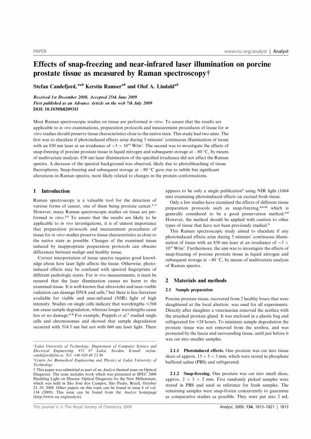
Effects of snap-freezing and near-infrared laser illumination on porcineprostate tissue as measured by Raman spectroscopy†
Stefan Candefjord,*ab Kerstin Ramserab and Olof A. Lindahlab
Received 1st December 2008, Accepted 25th June 2009
First published as an Advance Article on the web 7th July 2009
DOI: 10.1039/b820931f
Most Raman spectroscopic studies on tissue are performed in vitro. To assure that the results are
applicable to in vivo examinations, preparation protocols and measurement procedures of tissue for in
vitro studies should preserve tissue characteristics close to the native state. This study had two aims. The
first was to elucidate if photoinduced effects arise during 5 minutes’ continuous illumination of tissue
with an 830 nm laser at an irradiance of �3 � 1010 W/m2. The second was to investigate the effects of
snap-freezing of porcine prostate tissue in liquid nitrogen and subsequent storage at �80 �C, by means
of multivariate analysis. 830 nm laser illumination of the specified irradiance did not affect the Raman
spectra. A decrease of the spectral background was observed, likely due to photobleaching of tissue
fluorophores. Snap-freezing and subsequent storage at �80 �C gave rise to subtle but significant
alterations in Raman spectra, most likely related to changes in the protein conformations.
1 Introduction
Raman spectroscopy is a valuable tool for the detection of
various forms of cancer, one of them being prostate cancer.1–3
However, many Raman spectroscopic studies on tissue are per-
formed in vitro.2,4 To assure that the results are likely to be
applicable to in vivo investigations, it is of utmost importance
that preparation protocols and measurement procedures of
tissue for in vitro studies preserve tissue characteristics as close to
the native state as possible. Changes of the examined tissue
induced by inappropriate preparation protocols can obscure
differences between malign and healthy tissue.
Correct interpretation of tissue spectra requires good knowl-
edge about how laser light affects the tissue. Otherwise, photo-
induced effects may be confused with spectral fingerprints of
different pathologic states. For in vivo measurements, it must be
ensured that the laser illumination causes no harm to the
examined tissue. It is well-known that ultraviolet and near-visible
radiation can damage DNA and cells,5 but there is less literature
available for visible and near-infrared (NIR) light of high
intensity. Studies on single cells indicate that wavelengths #568
nm cause sample degradation, whereas longer wavelengths cause
less or no damage.6–8 For example, Puppels et al.7 studied single
cells and chromosomes and showed that sample degradation
occurred with 514.5 nm but not with 660 nm laser light. There
appears to be only a single publication9 using NIR light (1064
nm) examining photoinduced effects on excised fresh tissue.
Only a few studies have examined the effects of different tissue
preparation protocols such as snap-freezing,4,9,10 which is
generally considered to be a good preservation method.4,9
However, the method should be applied with caution to other
types of tissue that have not been previously studied.9
This Raman spectroscopic study aimed to elucidate if any
photoinduced effects arise during 5 minutes’ continuous illumi-
nation of tissue with an 830 nm laser at an irradiance of �3 �1010 W/m2. Furthermore, the aim was to investigate the effects of
snap-freezing of porcine prostate tissue in liquid nitrogen and
subsequent storage at �80 �C, by means of multivariate analysis
of Raman spectra.
2 Materials and methods
2.1 Sample preparation
Porcine prostate tissue, recovered from 2 healthy boars that were
slaughtered at the local abattoir, was used for all experiments.
Directly after slaughter a veterinarian removed the urethra with
the attached prostate gland. It was enclosed in a plastic bag and
refrigerated for <24 hours. To minimize sample degradation the
prostate tissue was not removed from the urethra, and was
protected by the fascia and surrounding tissue, until just before it
was cut into smaller samples.
2.1.1 Photoinduced effects. One prostate was cut into tissue
slices of approx. 15 � 5 � 3 mm, which were stored in phosphate
buffered saline (PBS) and refrigerated.
2.1.2 Snap-freezing. One prostate was cut into small slices,
approx. 2 � 3 � 2 mm. Five randomly picked samples were
stored in PBS and used as reference for fresh samples. The
remaining samples were snap-frozen concurrently to guarantee
as comparative studies as possible. They were put into 2 mL
aLule�a University of Technology, Department of Computer Science andElectrical Engineering, 971 87 Lule�a, Sweden. E-mail: [email protected]; Tel: +46 920 49 23 86bCentre for Biomedical Engineering and Physics at Lule�a University ofTechnology
† This paper was submitted as part of an Analyst themed issue on OpticalDiagnosis. The issue includes work which was presented at SPEC 2008Shedding Light on Disease: Optical Diagnosis for the New Millennium,which was held in Sao Jos�e dos Campos, Sao Paulo, Brazil, October25–29, 2008. Other papers on this topic can be found in issue 6 of vol.134 (2009). This issue can be found from the Analyst homepage(http://www.rsc.org/analyst).
This journal is ª The Royal Society of Chemistry 2009 Analyst, 2009, 134, 1815–1821 | 1815
PAPER www.rsc.org/analyst | Analyst

cryovials and lowered into liquid nitrogen. To avoid local heat-
ing the cryovials were constantly moved during the freezing.
They were then stored at �80 �C. Before measurement the snap-
frozen samples were allowed to passively thaw immersed in PBS.
2.2 Raman spectroscopy
ARaman micro spectrometer (Renishaw system 2000), equipped
with a 300 mW 830 nm laser and a water dip objective (Nikon
NIR Apo 60�/1.0 W), was used for all experiments. This spec-
trometer has two acquisition modes: the extended mode, where
a broad spectral window (in this study from 400–1800 cm�1) is
acquired by directing the Raman scattered light by a moving
prism onto the grating; or the static mode, where fast spectral
acquisition is recorded with a static prism. This mode only
enables a small spectral window of �500 cm�1. The irradiance
onto the samples was �3 � 1010 W/m2. The spectrometer was
calibrated for wavelength shift daily by using a single Raman
band (520 cm�1) from a silicon wafer as reference.
2.3 Measurement procedure
The samples were immersed in PBS during the measurements to
prevent dehydration of the tissue, which could disrupt the
protein vibrational modes.9
2.3.1 Investigation of photoinduced effects. The integration
time was set to 10 s in the static mode to enable short measure-
ment times. Spectra were acquired subsequently from the same
tissue spot during the first minute, to capture rapidly occurring
effects, and thereafter less frequently during an additional 4 min.
To guarantee good signal quality, the microscope focus was
moved 20 mm into the sample with a motorized z-stage. The
samples were immobilized with needles. A bright-field micro-
scope image was taken before and after each measurement series
to ensure that subsequent spectra were taken at the same tissue
spot. All measurement series were reproduced five times and
carried out within 4 days after slaughter.
2.3.2 Investigation of snap-freezing effects. The Raman signal
was integrated for 30 s and measured over a spectral range of
400–1800 cm�1. The microscope focus was moved approx. 10–20
mm into the sample. Five samples were measured on day 1 and
used as a reference of fresh samples. The snap-frozen samples
were measured after 5, 26 and 81 days of storage to investigate if
prolonged storage at �80 �C affected the tissue. Five samples
each were measured on day 5, 26 and 81. Each sample was
measured at 5 randomly chosen spots.
2.4 Preprocessing
Spectral spikes due to cosmic rays were removed prior to anal-
ysis. Correction for the energy sensitivity of the spectrometer was
performed by measuring the spectrum of a calibrated light source
and calculating the intensity wavenumber response curve. Each
Raman spectrum was lightly filtered by the noise-reduction
algorithm by Eilers.11 The background was automatically sub-
tracted using the algorithm by Cao et al.,12 which fits a piecewise
modified polynomial to the spectrum. The spectra were vector
normalized so that their integrated areas were equal. All
preprocessing algorithms, except the one by Eilers,‡ were written
in-house and implemented in Matlab (version R2007b including
Statistics Toolbox version 6.1).
2.5 Multivariate analysis on snap-freezing data
The preprocessed Raman spectra of fresh and snap-frozen tissues
were compared by means of multivariate analysis.13 Three
analogous analyses were carried out, fresh tissue was compared
to tissue that had been preserved at�80 �C for 5, 26, and 81 days.
Principal component analysis13 (PCA) on unstandardizedx data
was used as a first step to reduce the dimensionality of each data
set. The first 10 principal components (PCs) were kept. Next, it
was evaluated if there was any significant difference between the
multivariate means of the PC scores for fresh and snap-frozen
tissues. An adapted version of the original test proposed by
Kim,14 described by Lix et al.,15 was used. In the modified
version, trimmed means and Winsorized variance–covariance
replace the standard formulas. Trimming between 10 and 20% is
recommended,15 and in this study 15% was chosen.
If a significant difference was found between the multivariate
means of the two groups, univariate tests of the equality of means
of the individual PC scores were performed. This was done to
elucidate which PCs contributed strongly to the significant
multivariate difference. Yuen’s test16 was used for this purpose.
Matlab was used for the multivariate analysis, and most of the
tools were written in-house. A value of p < 0.05 was regarded as
statistically significant. It was assumed that the experimental
design was completely randomized and that the observations
were independent. Minitab (version 15.1.20.0) was used to check
the validity of the assumption of independency by means of
testing if significant autocorrelations17 were present.
3 Results
3.1 Photoinduced effects
No changes in the preprocessed Raman spectra due to the laser
illumination during 5 min were observed. This was evaluated
across the wavelength interval �400–1800 cm�1, requiring three
measurement series using the static mode. Fig. 1 shows the first
spectrum of a measurement series from 459 to 961 cm�1. Fig. 2
shows difference spectra for this series. No residual Raman peaks
were seen in difference spectra (n ¼ 5).
The total intensity of the background, calculated by inte-
grating the fitted piecewise modified polynomial that was sub-
tracted from all preprocessed spectra, diminished with increased
laser illumination time. Fig. 3(a) shows a typical example of the
diminishing background. The total intensity of the Raman
signal, i.e. the integral of un-normalized background-reduced
spectra, was unaltered by the laser illumination. Only random
fluctuations were seen, as shown in Fig. 3(b) and confirmed by
Fig. 2.
‡ Eilers has implemented the algorithm in Matlab and made it availablevia the Internet. See DOI: 10.1021/ac034173t.
x The variables were not scaled by dividing them with their standarddeviation.
1816 | Analyst, 2009, 134, 1815–1821 This journal is ª The Royal Society of Chemistry 2009

3.2 Snap-freezing
The first 10 PCs, explaining almost 90% of the variance, were
selected for further evaluation. A Pareto chart for the PCA of
fresh tissue and snap-frozen tissue stored for 5 days is shown in
Fig. 4. The corresponding plots for snap-frozen tissue stored 26
and 81 days were similar (data not shown).
Applying the modified Kim’s test on the multivariate means of
the PC scores showed a significant difference between the spectra
of the fresh and the snap-frozen tissue. The p-values obtained
were 1 � 10�7, 2 � 10�9 and 2 � 10�6 for snap-frozen tissue
stored at�80 �C for 5, 26 and 81 days, respectively, as compared
to fresh tissue. To elucidate which PCs gave rise to the multi-
variate difference Yuen’s univariate test was used on the indi-
vidual PCs. The scores of a few PCs for each measurement series
were significantly different. The p-values are shown in Table 1.
The accompanying PCs to the significant scores are plotted in
Fig. 1 The first Raman spectrum of one of the measurement series
evaluating 459–961 cm�1.
Fig. 2 Difference spectra for one measurement series. The spectra are
spatially offset for clarity and plotted in order of increasing accumulated
laser illumination from bottom to top. All spectra were compared to the
spectrum in Fig. 1.
Fig. 3 (a) The total intensity of the spectral background decreased with
the laser illumination time. (b) The total intensity of the Raman signal did
not change with the laser illumination time, only random fluctuations
were seen.
This journal is ª The Royal Society of Chemistry 2009 Analyst, 2009, 134, 1815–1821 | 1817

Fig. 5, from which some common characteristics due to snap-
freezing can be listed (tentative assignments from refs 18 and 19):
� decreased intensity of the phenylalanine (1006 cm�1) and
tryptophan (1548 and 760 cm�1) peaks;
� the amide I peak is shifted: fresh tissue yields a more intense
signal towards �1690 cm�1, whereas snap-frozen tissue shows
higher intensity towards �1660 cm�1;
� increased intensity at�1441 and �1299 cm�1, which may be
assigned to various CH2/CH vibrations of lipids and/or proteins;
� the amide III peak at �1244 cm�1 is decreased.
The changes are subtle and could not be seen when comparing
mean spectra. Fig. 6 compares two spectra for day 26 where the
differences are relatively large. These spectra were selected
because their PC5 scores differed markedly.
No signs that the PC scores were time dependent were seen
when studying the autocorrelation function in Minitab; the
assumption of independent observations was thus valid.
Analyses comparing snap-frozen tissue stored at �80 �C for
different time-spans were also performed. They showed signifi-
cant differences between these groups. The p-values obtained
applying the modified Kim’s multivariate test were in the order of
102–106 larger than the p-values obtained comparing fresh and
snap-frozen tissues.
Fig. 4 Pareto chart showing the amount of variance explained by each
PC, and the accumulated explained variance, for fresh tissue and snap-
frozen tissue stored for 5 days.
Table 1 The p-values obtained when Yuen’s test was applied on the two group means of the individual PC scores, for snap-frozen as compared to freshtissue. p-values < 0.05 have been written in bold
Storage time
PC number
PC1 PC2 PC3 PC4 PC5 PC6 PC7 PC8 PC9 PC10
5 days 0.51 0.19 0.11 0.014 0.63 0.56 0.0074 0.12 0.26 0.3426 days 0.56 0.31 0.056 0.47 0.0004 0.17 0.36 0.037 0.93 0.6381 days 0.24 0.90 0.12 0.066 0.57 0.024 0.82 0.22 0.22 0.033
Fig. 5 The calculated PCs whose scores were proven to be significantly
different for fresh and snap-frozen tissues. Fresh tissue obtained higher
scores of these PCs. Note that PC8 for day 26 has been inverted because
snap-frozen tissue obtained higher scores of this PC.
1818 | Analyst, 2009, 134, 1815–1821 This journal is ª The Royal Society of Chemistry 2009

4 Discussion
4.1 Photoinduced effects
No photoinduced effects on the Raman signal were observed at
an irradiance of �3 � 1010 W/m2 at 830 nm during 5 min.
Subsequent spectra were captured at relatively short intervals to
study if effects occurred rapidly. To get a reasonable signal
quality the integration time could not be less than 10 s.
Measurements were acquired temporarily closer than in
comparable studies.6,7,9 The total time was limited to 5 min as
relevant integration times usually are <1 min. Our results agree
with those of Notingher et al.6 who used 785 nm illumination at
an irradiance in the same order of magnitude for studying indi-
vidual cells. Shim and Wilson9 studied excised tissue using
1064 nm at an irradiance of �2 � 107 W/m2 and found no
evidence of heat damage in fat, muscle or liver. In lung tissue they
observed changes in the microstructure.
The spectral background diminished with increased illumina-
tion time. It has been shown that autofluorescence is generated
mainly by a few tissue fluorophores such as flavins, nicotinamide
adenine dinucleotide, aromatic acids such as tryptophan, tyro-
sine and phenylalanine, and porphyrins.20 Which molecular
species that are involved depend on the excitation wavelength, as
shown in the ultraviolet and the visible wavelength range.21,22
Only a few studies deal with NIR excitation, but it has been
suggested that in the NIR region, the intrinsic fluorescence is
primarily caused by porphyrins.23 Photobleaching of tissue flu-
orophores in general and porphyrins in particular is a well-
known phenomenon.24,25 Hence, in the present study, it is likely
that the registered fluorescence background and its decrease was
due to the myoglobin and hemoglobin present in the prostate
tissue. However, other fluorophores cannot be excluded.
4.2 Snap-freezing
4.2.1 Sample preparation. To isolate the effects of snap-
freezing the frozen and the fresh tissues should be handled as
similarly as possible, and tissue degradation should be mini-
mized. Prior to snap-freezing, the prostate was protected by the
fascia and adjacent tissue that surround the gland. As the pros-
tate was cut into small samples, focus was on minimizing the time
the tissue was exposed to air.
Ideally, to maintain conditions as close to the in vivo state as
possible, tissue should be snap-frozen immediately after being
removed from the animal body. However, this also requires that
the samples used as a reference of fresh samples can be measured
immediately. This was not feasible in the present study since the
laboratory facility and the abattoir were not at the same location.
4.2.2 Preprocessing. To extract the Raman signal objectively
all preprocessing was computerized. A light smoothing was
employed that reduced the noise efficiently while minimizing
distortion of the Raman peaks. The background-reduction
algorithm by Cao et al. was chosen because it selects the poly-
nomial orders of the piecewise polynomial that is fitted to the
background based on the fluorescence-to-signal ratio.12
Potentially large differences between the backgrounds of
different spectra may affect the results, since no background-
reduction algorithm can perfectly differentiate the Raman signal.
However, assuming that the fluorescent species are uniformly
present throughout the tissue, little variation is expected. The
spectral background was in fact consistent. This was checked by
plotting and comparing all backgrounds that were subtracted
from the spectra in the preprocessing (data not shown). PCA on
the backgrounds confirmed this, showing that >98% of the total
variance was explained by a single PC.
4.2.3 Multivariate analysis. PCA was performed on unstan-
dardized data since all variables had the same unit and the largest
standard deviations in the spectra coincided with the Raman
peaks. Only the 10 first PCs were selected for further exploration
since the aim was to examine the main differences between fresh
and snap-frozen tissues. The variance of all these PCs was much
higher than the variance of the original variables, justifying their
inclusion. It could be argued that more than 10 PCs should have
been included. However, when more than 10 PCs were included,
the results showed even stronger significant differences between
the multivariate means of fresh and snap-frozen tissues in all
comparisons. For example, the p-value obtained for comparing
snap-frozen tissue stored at �80 �C to fresh tissue was 3 � 10�10
when including 20 PCs, explaining about 94% of the total vari-
ance, as compared to 1 � 10�7 when 10 PCs were included.
This study examined macroscopically thick samples, hence
changes due to the freezing process should preferably be inves-
tigated using homogenous tissues. �O Faol�ain et al.4 chose to
examine tissue from the placenta due to its homogenous nature
to study the effects of freezing. However, it cannot be excluded
that different tissue types react differently from the snap-freezing
process. Furthermore, the use of thin-section microscopy would
have permitted histopathologic, and probably also spectro-
scopic,26 identification of different tissue types. However, that
was not an option as preparation of thin sections affects the
tissue and hence alters the result. To study thick slices of heter-
ogenous tissues, such as prostate tissue,26 necessitates the use of
statistical methods that can extract the changes due to the
freezing process in a heterogenous set of spectra. The
Fig. 6 A spectrum on fresh (blue) as compared to snap-frozen prostate
tissue (red) for day 26. Note, for example, that the phenylalanine (1004
cm�1) and tryptophan (758 cm�1) peaks are increased for fresh tissue.
These peaks are prominent in PC5, see Fig. 5.
This journal is ª The Royal Society of Chemistry 2009 Analyst, 2009, 134, 1815–1821 | 1819

heterogeneity of the tissue explains why the first 3–5 PCs, which
made up a large percentage of the total variance as exemplified in
Fig. 4, did not show a statistical difference between fresh and
snap-frozen tissues, as seen in Table 1. It is plausible that these
PCs reflect the variance due to different tissue types, which
indicates that the spectral variance due to the heterogenous
prostate tissue is greater than the relatively small but nevertheless
detectable variance between fresh and snap-frozen tissues.
The standard test for comparing multivariate means, Hotel-
ling’s T2, exhibits a high type I error rate when the assumptions
of multivariate normality and equal variance–covariance
matrices are violated.15,27 Univariate Anderson–Darling tests28
and normal probability plots showed that it was not reasonable
to assume a multivariate normal distribution, since some of the
PCs were not normally distributed. In the aggregate it might be
argued that the departures from normality were not so severe,
but a stringent analysis cannot rely on tests that are sensitive to
non-normality. Fortunately, alternative robust tests that
outperform the T2 statistic are available.15,27 A procedure that
shows good control of the type I error rate under a wide variety
of conditions,15,27 and does not assume equality of the variance–
covariance matrices, is the approach suggested by Kim14 in 1992.
To further improve its robustness to non-normality, it is rec-
ommended that robust estimators of mean value and variance–
covariance are used.15 Following Lix et al.,15 Kim’s test was
adapted using trimmed means and Winsorized variance–covari-
ance. The modified test is very robust to departures from
normality and variance–covariance heterogeneity.15
An analogous line of argument applies to the univariate testing
of the equality of means of the individual PC scores. Because
some PCs were non-normally distributed and heteroscedasticity,
as evaluated by the Levene29 test in Matlab, was sometimes
evident, a robust test had to be used. The choice fell upon the
two-sided trimmed t statistic for unequal population variances
proposed by Yuen in 1974,16 which is very robust to hetero-
scedasticity and non-normality.30
4.2.4 Observed changes. Subtle significant alterations, mainly
related to protein bands, as seen in Fig. 5, were found when snap-
frozen tissue was compared to fresh tissue. A possible explana-
tion is that the snap-freezing/thawing process alters the protein
conformations. The fact that the amide I peak is shifted towards
lower wavenumbers for snap-frozen tissue indicates changes in
the secondary protein structure, namely unravelling of b-sheets.18
This might also explain the lowered intensity at 1244 cm�1, since
the amide III peak is located at 1227–1247 cm�1 for the b-sheet
formation.18 Furthermore, proteins in b-sheet conformation
have a peak at 1002 cm�1, which was clearly reduced in snap-
frozen tissue. There were also changes in the region 500–
550 cm�1, which can be assigned to disulfide bridges and which
are related to a change in the tertiary protein structure.18
�O Faol�ain et al.4 evaluated freezing of tissue from the placenta
using OCT medium. They noted that freezing induced substan-
tial changes at 1002 cm�1, 1447 cm�1 and 1637 cm�1. They related
these changes to depolymerization of the cellular cytoskeleton,
which would result in unravelling of the secondary protein
structure, and that agrees with our explanation. However, they
observed substantial changes of spectra, and in contrast to our
findings, they found a decrease of intensity at 1441 cm�1. They
used a 514.5 nm laser at an irradiance of approx. 3 � 109 W/m2,
which could have induced photoinduced effects. Shim and
Wilson9 examined snap-freezing and OCT freezing of several
different tissues from hamster using 1064 nm excitation light.
They concluded that both freezing methods ‘provided adequate
preservation of biochemical composition’, although they noted
changes of the intensity ratio I1590/I1655 for several tissue types.
The differences between studies investigating freezing emphasize
that the results for one tissue type may not be fully valid for
another.
The analyses comparing snap-frozen tissue stored at �80 �Cfor different time-spans showed statistically significant differ-
ences between these groups. However, the difference between
fresh and snap-frozen tissues was much larger than variations
between snap-frozen groups. Thus, the main differences prob-
ably arise when the samples are snap-frozen or during thawing.
Many in vitro studies investigating, for example, changes in
prostate tissue induced by cancer use snap-freezing as a preser-
vation method. More knowledge of the snap-freezing process is
needed to elucidate if the results of such studies also apply to in
vivo conditions. Although the changes due to snap-freezing
found in this study are subtle, a change in protein conformation
might potentially have a large influence on the interpretation of
findings concerning in vitro studies.
5 Conclusion
The 830 nm laser irradiation of PBS-immersed porcine prostate
tissue of high irradiance does not appear to affect Raman
spectra. The spectral background decreased with increased laser
illumination time, and this was probably caused by photo-
bleaching of tissue fluorophores. For techniques that incorporate
the background information into discriminative algorithms it
could be worth investigating this in further detail.
Snap-freezing of porcine prostate tissue seems to alter the
protein conformation. The changes could not be seen comparing
mean spectra, which can be explained by the inhomogeneity of
the prostate tissue. Although the changes in the spectra on the
whole were subtle, changes of the protein structure may affect in
vitro measurements, as compared to the in vivo situation. This is
especially important to consider for studies finding diagnostic
information in the Raman peaks related to protein conforma-
tion.
Acknowledgements
The authors wish to thank Professor Kerstin V€annman for
valuable discussions, and veterinarians Bertil Funck and Mats
Gustavsson for helping us to obtain prostate samples.
The study was funded by the Objective 2 Norra Norrland – EU
Structural Fund, and the Kempe Foundation.
References
1 M. D. Keller, E. M. Kanter and A.Mahadevan-Jansen, Spectroscopy,2006, 21, 33–41.
2 C. Krafft and V. Sergo, Spectroscopy, 2006, 20, 195–218.
1820 | Analyst, 2009, 134, 1815–1821 This journal is ª The Royal Society of Chemistry 2009

3 N. Stone, M. C. H. Prieto, P. Crow, J. Uff and A. W. Ritchie, Anal.Bioanal. Chem., 2007, 387, 1657–1668.
4 E. �O Faol�ain, M. B. Hunter, J. M. Byrne, P. Kelehan,M.McNamara,H. J. Byrne and F. M. Lyng, Vibrational Spectroscopy, 2005, 38, 121–127.
5 T. P. Coohill, M. J. Peak and J. G. Peak, Photochem. Photobiol., 1987,46, 1043–1050.
6 I. Notingher, S. Verrier, H. Romanska, A. E. Bishop, J. M. Polak andL. L. Hench, Spectroscopy, 2002, 16, 43–51.
7 G. J. Puppels, J. H. Olminkhof, G. M. Segers-Nolten, C. Otto,F. F. de Mul and J. Greve, Exp. Cell Res., 1991, 195, 361–367.
8 K. C. Neuman, E. H. Chadd, G. F. Liou, K. Bergman andS. M. Block, Biophys. J., 1999, 77, 2856–2863.
9 M.G.ShimandB.C.Wilson,Photochem.Photobiol., 1996,63, 662–671.10 C.M.Krishna,G.D.Sockalingum,L.Venteo,R.A.Bhat, P.Kushtagi,
M. Pluot and M. Manfait, Biopolymers, 2005, 79, 269–276.11 P. H. Eilers, Anal. Chem., 2003, 75, 3631–3636.12 A. Cao, A. K. Pandya, G. K. Serhatkulu, R. E. Weber, H. Dai,
J. S. Thakur, V. M. Naik, R. Naik, G. W. Auner, R. Rabah andD. C. Freeman, J. Raman Spectrosc., 2007, 38, 1199–1205.
13 D. E. Johnson, Applied multivariate methods for data analysts,Duxbury Press, New York, 1998.
14 S. J. Kim, Biometrika, 1992, 79, 171–176.15 L. M. Lix, H. J. Keselman and A. M. Hinds, Comput. Methods
Programs Biomed., 2005, 77, 129–139.16 K. K. Yuen, Biometrika, 1974, 61, 165–171.17 R. A. Johnson and D. W. Wichern, Applied Multivariate Statistical
Analysis, Prentice-Hall, Upper Saddle River, NJ, 4th edn, 1998.
18 A. Mahadevan-Jansen and R. R. Richards-Kortum, J. Biomed. Opt.,1996, 1, 31–70.
19 Z. Movasaghi, S. Rehman and I. U. Rehman, Applied SpectroscopyReviews, 2007, 42, 493–541.
20 L. C. Kwek, S. Fu, T. C. Chia, C. H. Diong, C. L. Tang andS. M. Krishnan, Appl. Opt., 2005, 44, 4004–4008.
21 Z. Huang, H. Zeng, I. Hamzavi, A. Alajlan, E. Tan, D. I.McLean andH. Lui, J. Biomed. Opt., 2006, 11, 034010.
22 G. Zhang, S. G. Demos and R. R. Alfano, Lasers Life Sci., 1999, 9,1–16.
23 Z. Huang, H. Lui, D. I. McLean, M. Korbelik and H. Zeng,Photochem. Photobiol., 2005, 81, 1219–1226.
24 M. S. Viegas, T. C. Martins, F. Seco and A. do Carmo, Eur. J.Histochem., 2007, 51, 59–66.
25 D. J. Robinson, H. S. de Bruijn, N. van der Veen, M. R. Stringer,S. B. Brown and W. M. Star, Photochem. Photobiol., 1998, 67, 140–149.
26 D. C. Fernandez, R. Bhargava, S. M. Hewitt and I. W. Levin, Nat.Biotechnol., 2005, 23, 469–474.
27 W. T. Coombs, J. Algina and D. O. Oltman, Review EducationalResearch, 1996, 66, 137–179.
28 T. W. Anderson and D. A. Darling, Ann. Math. Statist., 1952, 193–212.
29 H. Levene, in Contributions to probability and statistics: Essays inhonor of Harold Hotelling, ed. I. Olkin, Stanford University Press,Stanford, CA, 1960, pp. 278–292.
30 H. J. Keselman, R. R. Wilcox and R. O. S. Kowalchuk, BiometricalJournal, 2002, 44, 478–489.
This journal is ª The Royal Society of Chemistry 2009 Analyst, 2009, 134, 1815–1821 | 1821

104
Paper C
Combining fibre optic Ramanspectroscopy and tactile resonance
measurement for tissuecharacterization
Authors:Stefan Candefjord, Morgan Nyberg, Ville Jalkanen, Kerstin Ramser and Olof A. Lindahl
Paper originally published in:Measurement Science & Technology, vol. 21, 125801 (8 pp.), 2010.1
© 2010 IOP Publishing Ltd. Reproduced with permission.
1http://dx.doi.org/10.1088/0957-0233/21/12/125801
105

106
IOP PUBLISHING MEASUREMENT SCIENCE AND TECHNOLOGY
Meas. Sci. Technol. 21 (2010) 125801 (8pp) doi:10.1088/0957-0233/21/12/125801
Combining fibre optic Ramanspectroscopy and tactile resonancemeasurement for tissue characterizationStefan Candefjord1,2, Morgan Nyberg1,2, Ville Jalkanen2,3,Kerstin Ramser1,2 and Olof A Lindahl1,2
1 Department of Computer Science and Electrical Engineering, Luleå University of Technology, Luleå,Sweden2 Centre for Biomedical Engineering and Physics, Luleå University of Technology and Umeå University,Luleå and Umeå, Sweden3 Department of Applied Physics and Electronics, Umeå University, Umeå, Sweden
E-mail: [email protected]
Received 10 June 2010, in final form 5 October 2010Published 15 November 2010Online at stacks.iop.org/MST/21/125801
AbstractTissue characterization is fundamental for identification of pathological conditions. Ramanspectroscopy (RS) and tactile resonance measurement (TRM) are two promising techniquesthat measure biochemical content and stiffness, respectively. They have potential tocomplement the golden standard—histological analysis. By combining RS and TRM,complementary information about tissue content can be obtained and specific drawbacks canbe avoided. The aim of this study was to develop a multivariate approach to compare RS andTRM information. The approach was evaluated on measurements at the same points onporcine abdominal tissue. The measurement points were divided into five groups bymultivariate analysis of the RS data. A regression analysis was performed and receiveroperating characteristic (ROC) curves were used to compare the RS and TRM data. TRMidentified one group efficiently (area under ROC curve 0.99). The RS data showed that theproportion of saturated fat was high in this group. The regression analysis showed thatstiffness was mainly determined by the amount of fat and its composition. We concluded thatRS provided additional, important information for tissue identification that was not providedby TRM alone. The results are promising for development of a method combining RS andTRM for intraoperative tissue characterization.
Keywords: tissue characterization, multivariate analysis, Raman spectroscopy, tactileresonance measurement, biological tissues
List of parameters and abbreviations
d impression depth�f resonance frequency shiftF impression forceHCA hierarchical cluster analysisPC principal componentPCA principal component analysisROC receiver operating characteristicRS Raman spectroscopy
S stiffness parameterTRM tactile resonance measurement
1. Introduction
Tissue characterization is very important for the determinationof pathological conditions such as cancer. The golden standardis histological analysis using bright field microscopy. Themethod allows a trained observer to identify diseased tissuethrough staining of tissue samples. However, the methodis subjective and the inter- and intra-observer agreement is
0957-0233/10/125801+08$30.00 1 © 2010 IOP Publishing Ltd Printed in the UK & the USA

Meas. Sci. Technol. 21 (2010) 125801 S Candefjord et al
unsatisfactory [1]. Furthermore, it is time-consuming andcannot be used in vivo. Therefore, complementary methodsare needed. There are several promising technologies forprecise and swift tissue characterization [1–5]. However, toour knowledge, none are ready to be used clinically at present.
Recently, the combination of different techniques hasgained increased interest [6]. We have earlier suggestedthat it may be beneficial to analyze both the biochemicaland biomechanical properties of tissue to achieve efficientcharacterization [1, 7]. Raman spectroscopy (RS) and tactileresonance measurement (TRM) measure the biochemicalcontent and the stiffness of tissue, respectively. Theseexperimental methods have shown promising results in vitrofor tissue characterization [2, 4], e.g. prostate cancer detection[1, 4]. Used together, the two methods may compensate forthe specific drawbacks of each method alone, e.g. the limitedpenetration depth of current fibre optic RS probes [8] andTRM’s lack of detailed information about tissue content [9].
RS is an optical method in which a beam ofmonochromatic light is directed at the examined material.The backscattered light forms a spectrum reflecting thebiochemical content of the tissue [10]. By using multivariateanalysis of the RS data many pathological conditions canbe recognized in an objective manner [11]. For example,several in vitro studies using RS microscope setups show thatdiagnostic algorithms can differentiate healthy and cancerousprostate tissue with high accuracy [12–16]. The methodalso holds promise for determining tumour aggressivity [12,15]. Recently, multivariate analysis of RS and infraredspectroscopic data has been used to characterize healthy tissueas a first step to develop a diagnostic algorithm [17, 18].Andrade et al [18] used clustering analysis to distinguishdifferent tissue types in normal colorectal samples.
RS can be performed using optical fibres to deliver theexciting laser beam and collect the Raman scattered signal.Crow et al used a fibre optic RS probe and differentiatedbenign and malignant prostate samples in vitro with an overallaccuracy of 86% [13]. RS has not yet become clinically usefuldue to the lack of suitable fibre optic probes [2], relativelylong acquisition times and concerns that the laser illuminationmay cause photo-induced degeneration [19]. Furthermore, RSusually requires that the measurements should be performedin darkness. It may be possible to overcome these problemsby combining RS with TRM.
The TRM mimics palpation since it senses the stiffness ofan object. TRM gives an objective reading of the stiffness, asopposed to the subjective manual palpation. The transducerof TRM is a resonance sensor element consisting of apiezoelectric ceramic. The resonance frequency shifts as theprobe is pressed against an object, and the shift (�f ) is relatedto the stiffness of the object [4]. TRM generates an ultrasonicwave in the tissue, and the method is more gentle and deep-sensing [20] than RS. Several medical TRM applications areunder development [4], e.g. breast cancer [21] and prostatecancer detection [9, 20, 22, 23]. In vitro studies show thathealthy glandular tissue and cancerous prostate tissue can bedifferentiated using TRM [9, 23]. Stiff prostate tissue indicatesthe presence of a tumour, although increased stiffness is not
necessarily due to cancer. TRM alone cannot yet distinguishbetween cancerous tissue and stiff healthy prostate tissue suchas stroma and prostate stones [9]. With the addition of RS toTRM the diagnostic accuracy may be improved.
Our long-term goal is to integrate RS and TRM into onesingle probe to be used clinically. For instance, the instrumentcould be a portable hand-held device used during radicalprostatectomy surgery to locate cancerous tissue in the surgicalmargins. The hand-held resonance sensor concept has recentlybeen demonstrated on tissue phantoms [22]. TRM would beused to scan the prostate tissue and localize stiff areas, whichmay indicate tumors. The suspicious areas would be analyzedby RS to be confirmed as healthy or diseased tissue. Diagnosticalgorithms will be developed that objectively can classify thetissue from the combined RS and TRM information.
A first step toward combining RS and TRM for tissuecharacterization is to compare measurements from the sametissue. The aim of this study was to develop a multivariateapproach to compare the RS information of biochemicalcontent to the TRM information of tissue stiffness.
2. Material and methods
2.1. Sample preparation
We chose to use porcine abdominal tissue for this study. Twopackages were purchased from the local grocery store andkept at 6 ◦C until sample preparation. Rectangular tissuesamples were cut 9 mm thick with approximately 40 and50 mm sides. The tissue samples were fixed to a 19 mm thickStyrofoam plate with needles. A total of four samples, twofrom each package, were prepared. The samples were takenout of the refrigerator 30 min before each measurement seriesto suppress temperature drift during the measurement run. Allmeasurements were performed at room temperature (25 ◦C ±0.8 ◦C). Phosphate buffered saline was applied with a softbrush to the freshly cut surface every fifth minute.
2.2. Measurements
2.2.1. Raman spectroscopy. A fibre optic RS probe [24](Machida Endoscope Co., Tokyo, Japan) was used. It had anouter diameter of 0.8 mm and incorporated a central deliveryfibre and eight surrounding collecting fibres. Optical filtersat the probe tip rejected Raman scattered light generated inthe delivery fibre. The fibre optic probe was connected toan RXN1 spectroscope with a continuous-wave InvictusTM
diode laser at 785 nm (both from Kaiser Optical Systems(KOSI), Ann Arbor, MI, USA). The system was calibratedfor wavelength shift and energy sensitivity using a calibrationsystem (HoloLab Calibration Accessory, KOSI). The outputeffect to the samples was adjusted to approximately 80 mW andthe signal was integrated for 30 s. Prior to each measurement,the probe tip was positioned as close to the sample as possiblewithout touching it. The ideal measurement distance for thistype of probe is 0.4 mm [24]. In this study, the approximatedistance was set by visual inspection using a magnifying glass.This was sufficient since good spectral quality was acquired ina range of several tenths of mm around the optimal distance.
2

Meas. Sci. Technol. 21 (2010) 125801 S Candefjord et al
The diameter of the laser spot on the sample at a distance of0.4 mm was estimated to be 0.3 mm [25].
2.2.2. Tactile resonance measurement. A tactile resonancesensor system consisting of a stepper motor, a position meterand a probe tip with force sensor and a piezoelectric element(Venustron R©Axiom Co. Ltd, Koriyama Fukushima, Japan)was used [9, 20, 22, 23, 26]. The piezoelectric element wasdivided into a driving part and a pick-up, which recorded theresonance frequency. The element was set into vibration by anelectronic feedback circuit that retained the phase shift at zero.The shift in resonance frequency occurring as the sensor ispressed against a measurement object is related to the stiffnessof the object [27].
The resonance frequency of the piezoelectric element was59 kHz before contact. The resonance frequency shift (�f ),impression force (F) and impression depth (d) were sampledat 200 Hz during measurements. The sensor tip was pressedmaximally 1.0 mm into the tissue at a speed of 1 mm s−1. Thetissue surface was detected through the large frequency shiftthat occurred upon contact. The radius of the hemisphericaltip was 2.5 mm.
2.2.3. Combined RS and TRM measurement setup. The RSand TRM probes were mounted above a computer-controlledtranslation stage (NRT150P1, three NRT100, BSC103,Thorlabs, Newton, NJ, USA), together with a digital camera(Canon Powershot S3 IS with close-up lens 500D and LAH-DC20 conversion lens adapter, Canon, Tokyo, Japan), figure 1.The Styrofoam plate with the tissue sample was fixed to thetranslation stage. A software program, developed in-house,was implemented in LabVIEWTM (National Instruments,Austin, TX, USA) and ensured that measurements with bothprobes were performed at the same locations on the tissuesample. The positions of the probes were calibrated beforethe measurements started, by aligning the probe tips with areference mark on the translation stage. Each tissue samplewas photographed and the position of the sample relative to thetranslation stage was recorded. The image was imported to theLabVIEWTM program and used to position the measurementpoints. A grid of 42 measurement points arranged in a 6 × 7matrix was overlaid on the image of each sample. The totalnumber of measurement points on the four samples was 168.The points were set 5.0 mm apart since this approximatelyequaled the diameter measured by the TRM probe at animpression depth of 0.6 mm [20]. The measurement runtime order was randomized with the constraint that spatiallyadjacent points were separated in time by at least oneintervening measurement. The total measurement time wasaround two hours, whereof the TRM measurements tookapproximately 30 min and the RS measurements 90 min.
2.3. Data preprocessing and analysis
Matlab R© (version R2009b including Statistics Toolbox version7.0, MathWorks Inc., Natick, MA, USA) was used for allpreprocessing and analysis. Algorithms included in Matlab R©
were used if possible. Additional algorithms were written and
321
456
IMAGE
ACQUIRED
GRID
CHOSEN
TRMSTIFFNESS
RSSPECTRA
Figure 1. A flow chart illustrating the measurement scheme. (1)Digital camera, (2) Venustron R© resonance sensor, (3) RS fibre opticprobe, (4) tissue sample, (5) Styrofoam plate, (6) translation stage.
implemented in Matlab R© in-house. Eilers’ algorithm [28] hasbeen made available for Matlab R© via the Internet.
2.3.1. Preprocessing and analysis of the RS data. Thespectral interval 600–1800 cm−1, referred to as the fingerprintregion [10], was selected for further analysis. Each spectrumwas lightly filtered by a noise-reduction algorithm, settingthe smoothing parameters d = 2 and λ = 10 [28]. Thefluorescence background was automatically subtracted byfitting a piecewise modified polynomial to each spectrum [29].The spectra were vector normalized so that the integratedintensity was equalized.
All 168 spectra measured on the four samples werecollected in one data set. Principal component analysis (PCA)[30] was used to reduce the dimensionality of the data. PCAprojects the data onto a new coordinate system so that the firstcoordinate describes as much of the variance as possible, thesecond coordinate explains as much of the remaining varianceas possible, and so on. The coordinates are called principalcomponents (PCs), and they are orthogonal to each other. Thevalues for the observations expressed in the new coordinatesystem are called PC scores. The preprocessed spectrawere analyzed using PCA, and a selected number of PCs wereretained. The reduced data set was then input to a hierarchicalcluster analysis (HCA) algorithm. The HCA automaticallydivided the spectra into groups, where spectra within the samegroup were similar to each other. Ward’s linkage [30] was usedto merge observations (spectra) close to each other, based onthe Euclidean distances between the observations.
The spectra were interpreted by tentatively assigningthe spectral features to specific molecular vibrations usinga database [31].
2.3.2. Analysis of the TRM data. The stiffness parameter S[N Hz−1] was calculated from �f , F and d:
S = ∂F/∂d
∂�f/∂d
, (1)
3

Meas. Sci. Technol. 21 (2010) 125801 S Candefjord et al
where ∂F/∂d and ∂�f /∂d were estimated numerically bylinear regression in an interval of d ± 0.1 mm. S was calculatedat d = 0.6 mm, representing the tissue stiffness near the surface[20]. S has previously been shown to be proportional toYoung’s modulus [26].
2.3.3. Combined measurements. A linear regression analysis[32] was performed to relate S to the PCs. S was taken asthe model response variable, whereas the PCs were the modelpredictor variables. A residual analysis of zero mean, constantvariance, time independence and normality was done for modelvalidation. The adjusted coefficient of multiple determinationR2
adj was used for model control and comparison [32].The accuracy of TRM to classify different tissue types
according to their stiffness was evaluated by the area under thereceiver operating characteristic (ROC) curve. The sensitivityand specificity at various stiffness threshold values werecalculated to construct the ROC curves. The sensitivityis the proportion of correct positive classification, and thespecificity is the proportion of correct negative classification.An area under the curve close to 1.0 indicates an excellentmethod, whereas an area of 0.5 indicates a noninformativemethod [33].
2.3.4. Statistics. The mean stiffness was calculated foreach group as defined by the cluster analysis of the RS data.The nonparametric Kruskal–Wallis test, followed by Tukey–Kramer’s multiple comparison test, were performed to testfor differences between groups of stiffness measurements.The Anderson–Darling test was used to test for normality.Statistical test results with p < 0.05 were consideredstatistically significant.
3. Results
3.1. RS measurements
The RS data were first analyzed using PCA. The first ten PCswere retained. These explained >99% of the total varianceof the RS data, whereof PC 1 alone explained 94%. Thespectra were divided into five groups as defined by the HCA,and they were labeled A, B, C, D and E. The mean spectra(figure 2) agreed well with published results on porcine tissue[34]. Analysis of the spectral peaks showed that group A wasmuscle tissue, D and E fat tissue, while B and C consisted ofboth muscle and fat tissue (figure 2). Group C contained alarger proportion of fat than group B. Spectra D and E weresimilar but the intensity of several peaks differed (figure 2(inset)). The major differences were assigned to differentvibrations in lipids [31]:
• Spectrum D had higher intensity than spectrum E at thepeaks at 1659 and 1265 cm−1. These peaks were assignedto C=C stretching and vibrations of the C=C and =C−Hbonds, respectively.
• Spectrum E had higher intensity than spectrum D at thepeaks at 1440, 1296, 1128 and 1062 cm−1. The first twopeaks were assigned to CH2/CH3 and CH2 vibrations,respectively. The peaks at 1128 and 1062 cm−1 wereboth due to C−C stretching.
Inte
nsity
(ar
b)
18001600140012001000800600
Raman shift (cm-1)
A (muscle)
B (fat/muscle)
C (fat/muscle)
D (fat)
E (fat)
Inte
nsit
y (a
rb)
1600140012001000
Raman shift (cm-1)
1659
14401296
1265
1062
|
1128
E–D
Figure 2. The mean Raman spectrum for each of groups A–E. Thespectra have been spatially offset for clarity. The inset shows thedifference between spectra E and D within 1000–1700 cm−1, wherethe major peaks were observed. These peaks have been labeled withtheir wavenumbers.
These differences indicated that group E contained a higherproportion of saturated fatty acids than group D [10]. Thecomposition of the fat differed between the two batches oftissue. One batch consisted only of fat from group D, whereasthe other batch consisted mainly of fat from group E (42 outof 44 measurement points).
PCs 1, 2 and 4 discriminated the different groups mostefficiently (figure 3). PC 1 was interpreted as being relatedto the proportion of fat tissue, PC 2 to the proportionof muscle tissue, whereas PC 4 described the amount ofsaturated/unsaturated fatty acids.
3.2. TRM measurements
The stiffness parameter S was calculated from the twoderivatives ∂F/∂d and ∂�f /∂d (illustrated in figure 4),according to equation (1). S was positively skewed (figure 5)with a mean of 0.40 mN Hz−1 and a standard deviation of0.24 mN Hz−1. For the majority of the measurement pointsS was <0.40 mN Hz−1, but some stiffer points on the tissuewere observed (figure 5).
4

Meas. Sci. Technol. 21 (2010) 125801 S Candefjord et al
−0.02
−0.01
0
0.01
0.02
−0.01
−0.005
0
0.005
0.01−4
−3
−2
−1
0
1
2
3
x 10−3
PC1PC2
PC4
A
B
C
D
E
Figure 3. A scatter plot of the scores of PC 1, 2 and 4 for all RSmeasurements. The group division (A–E) from the cluster analysisis shown by the different markers.
0 0.2 0.4 0.6 0.8 10
20
40
60
80
100
120
140
∂F/∂d = 90 mN/mm
F (
mN
)
d (mm)
∂F/∂d = 96 mN/mm
0 0.2 0.4 0.6 0.8 10
50
100
150
200
250
∂Δf/∂d = 223 mN/mm
Δf (
Hz)
d (mm)
∂Δf/∂d = 163 mN/mm
Figure 4. The impression force (F) and the frequency shift (�f )plotted against the impression depth (d) for two representativemeasurement points. The values of the derivatives ∂F/∂d and∂�f /∂d at d = 0.6 were estimated by calculating the line slopes inan impression depth interval of 0.5 to 0.7 mm, marked by crosses(+).
0 0.2 0.4 0.6 0.8 10
10
20
30
40
Bin
cou
nts
Stiffness parameter (mN/Hz)
Figure 5. A histogram of the stiffness parameter S distribution of allmeasurement points (n = 168). A higher value of S indicates stiffertissue.
S (
mN
/Hz)
Raman cluster classification
*
A (n=68) B (n=10) C (n=11) D (n=37) E (n=42)0
0.2
0.4
0.6
0.8
1
Figure 6. The mean stiffness of groups A–E calculated from theTRM measurements. The standard deviations are shown by the bars.The asterisk (∗) denotes significantly separated groups (p < 0.05).
Table 1. Model coefficients (βi) from the regression modelsbetween the stiffness parameter S and the Raman PCs. The fullmodel included all ten PCs. R2
adj is the adjusted coefficient ofmultiple determination. The asterisks (∗) mark the coefficients thatwere significant (p < 0.05). The significant model included the sixsignificant PCs. All model coefficient values are the standardizedmodel coefficients divided by their sum and given as a percentage.
Model coefficient, Full model, Significant model,βi (%) R2
adj = 0.673 R2adj = 0.669
β1 30∗ 33β2 −12∗ −14β3 2 –β4 28∗ 32β5 −7∗ −7β6 6∗ 7β7 2 –β8 2 –β9 −5 –β10 6∗ 7
3.3. Comparing RS with TRM measurements
Group E was significantly stiffer than the other groups(p < 0.05), whereas no significant difference was found amonggroups A–D (figure 6).
The estimated coefficients (βi) from the regressionanalyses gave the relative impact of the ith PC score onthe stiffness parameter S (table 1). A negative coefficientindicated that the specific PC decreased S. The residual
5
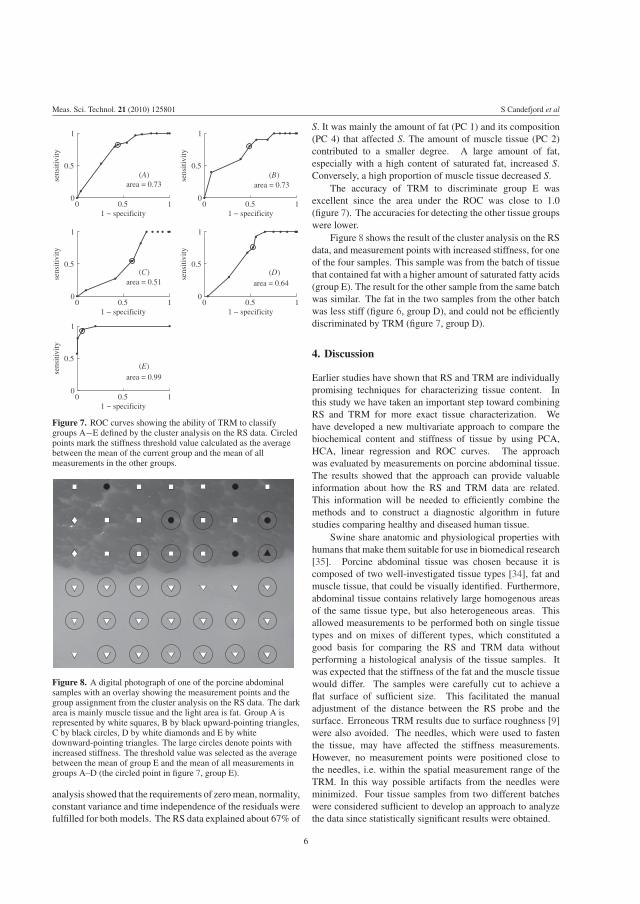
Meas. Sci. Technol. 21 (2010) 125801 S Candefjord et al
0 0.5 10
0.5
1
sens
itivi
ty
1 − specificity
area = 0.73
0 0.5 10
0.5
1
sens
itivi
ty
1 − specificity
area = 0.99
0 0.5 10
0.5
1
sens
itivi
ty
1 − specificity
area = 0.64
0 0.5 10
0.5
1
sens
itivi
ty
1 − specificity
area = 0.73
0 0.5 10
0.5
1
sens
itivi
ty
1 − specificity
area = 0.51
(A) (B)
(C)
(E)
(D)
Figure 7. ROC curves showing the ability of TRM to classifygroups A−E defined by the cluster analysis on the RS data. Circledpoints mark the stiffness threshold value calculated as the averagebetween the mean of the current group and the mean of allmeasurements in the other groups.
Figure 8. A digital photograph of one of the porcine abdominalsamples with an overlay showing the measurement points and thegroup assignment from the cluster analysis on the RS data. The darkarea is mainly muscle tissue and the light area is fat. Group A isrepresented by white squares, B by black upward-pointing triangles,C by black circles, D by white diamonds and E by whitedownward-pointing triangles. The large circles denote points withincreased stiffness. The threshold value was selected as the averagebetween the mean of group E and the mean of all measurements ingroups A–D (the circled point in figure 7, group E).
analysis showed that the requirements of zero mean, normality,constant variance and time independence of the residuals werefulfilled for both models. The RS data explained about 67% of
S. It was mainly the amount of fat (PC 1) and its composition(PC 4) that affected S. The amount of muscle tissue (PC 2)contributed to a smaller degree. A large amount of fat,especially with a high content of saturated fat, increased S.Conversely, a high proportion of muscle tissue decreased S.
The accuracy of TRM to discriminate group E wasexcellent since the area under the ROC was close to 1.0(figure 7). The accuracies for detecting the other tissue groupswere lower.
Figure 8 shows the result of the cluster analysis on the RSdata, and measurement points with increased stiffness, for oneof the four samples. This sample was from the batch of tissuethat contained fat with a higher amount of saturated fatty acids(group E). The result for the other sample from the same batchwas similar. The fat in the two samples from the other batchwas less stiff (figure 6, group D), and could not be efficientlydiscriminated by TRM (figure 7, group D).
4. Discussion
Earlier studies have shown that RS and TRM are individuallypromising techniques for characterizing tissue content. Inthis study we have taken an important step toward combiningRS and TRM for more exact tissue characterization. Wehave developed a new multivariate approach to compare thebiochemical content and stiffness of tissue by using PCA,HCA, linear regression and ROC curves. The approachwas evaluated by measurements on porcine abdominal tissue.The results showed that the approach can provide valuableinformation about how the RS and TRM data are related.This information will be needed to efficiently combine themethods and to construct a diagnostic algorithm in futurestudies comparing healthy and diseased human tissue.
Swine share anatomic and physiological properties withhumans that make them suitable for use in biomedical research[35]. Porcine abdominal tissue was chosen because it iscomposed of two well-investigated tissue types [34], fat andmuscle tissue, that could be visually identified. Furthermore,abdominal tissue contains relatively large homogenous areasof the same tissue type, but also heterogeneous areas. Thisallowed measurements to be performed both on single tissuetypes and on mixes of different types, which constituted agood basis for comparing the RS and TRM data withoutperforming a histological analysis of the tissue samples. Itwas expected that the stiffness of the fat and the muscle tissuewould differ. The samples were carefully cut to achieve aflat surface of sufficient size. This facilitated the manualadjustment of the distance between the RS probe and thesurface. Erroneous TRM results due to surface roughness [9]were also avoided. The needles, which were used to fastenthe tissue, may have affected the stiffness measurements.However, no measurement points were positioned close tothe needles, i.e. within the spatial measurement range of theTRM. In this way possible artifacts from the needles wereminimized. Four tissue samples from two different batcheswere considered sufficient to develop an approach to analyzethe data since statistically significant results were obtained.
6

Meas. Sci. Technol. 21 (2010) 125801 S Candefjord et al
The TRM measurements were performed before the RSmeasurements (figure 1). The reason was that the laserirradiation may affect the stiffness of the tissue, e.g. viadehydration, whereas the TRM was unlikely to induce anychanges of the biochemical content.
The tissue characteristics were first described by usingthe RS data to divide the measurement points into groups withsimilar tissue. The tissue description given by TRM was lessdetailed and allowed less tissue discrimination than that givenby the RS. Cluster analysis of the RS data is an efficient toolto distinguish different tissue types [18]. HCA enables anunsupervised automatic division of the measurement pointsinto a selected number of groups. The number of groupsthat is appropriate cannot be determined in advance [36]. Ingeneral, more details are revealed when the number of groupsis increased, but larger tissue structures may then be disguised.After comparing cluster analyses using 2–9 groups, five groupswere chosen in this study. The Raman spectral data showedthat the measurement points were divided into five distinctgroups (figures 2 and 3). In particular, D and E were clearlyseparated in the PC scores plot (figure 3). These groups weremerged using fewer than five clusters in the HCA. Choosingmore than five clusters did not aid the comparison betweenTRM and RS since the mean stiffness of the new subgroupsdid not differ significantly.
Visual inspection of the samples (figure 8) agreed withinterpretations of the mean spectra (figure 2). TRM wasexpected to discriminate fat from muscle tissue due todifferences in stiffness. However, it only separated onetype of fat (group E) from the muscle tissue. The spectraldata showed that group E contained a larger proportion ofunsaturated fat than group D. This agreed with the stiffnessmeasurements showing that group E was stiffer than groupD since saturated fat is harder than unsaturated fat at roomtemperature [37]. The regression analysis (table 1) showed thatthe biochemical content explained a large proportion (67%),but not all, of the stiffness parameter S. This indicated thatthere was stiffness variation that could not be explained byRS, and that TRM and RS give complementary informationfor tissue characterization.
The diagnostic accuracy for identifying group E wassatisfactory using TRM. However, the other groups could notbe distinguished efficiently by TRM (figure 7). The Ramanspectral data showed marked differences between groups A–D (figures 2 and 3). This suggests that RS added valuableinformation to TRM to aid in the differentiation into tissuegroups A–D.
If the measurement volumes of the two sensors hadbeen more equal, a better model agreement (table 1) mayhave been obtained. RS fibre optic probes measuring thebackscattered light have penetration depths of the order of100 μm [8], whereas the sensing depth of the TRM probehas been estimated to be about 2.5–4.5 mm at an impressiondepth of 0.6 mm [20]. The lateral measurement areas alsodiffer; they are estimated to be ∼0.2 mm2 for the RS probe[25] and ∼20 mm2 for the TRM probe [20]. The areas withmainly muscle tissue visually appeared more heterogeneousthan the areas with fat (figure 8). In heterogeneous areas TRM
measured on several different tissue types at once (upper partof figure 8), due to its relatively large sensing volume. Thisprobably impaired TRM’s ability to distinguish between them(figure 6). Measurement points with increased stiffness thatdid not belong to group E seemed to be positioned close toareas with high fat content (figure 8). The increased stiffnessmay have been due to the adjacent fat, which was not sensedby the RS probe. Four of these points were assigned togroup A, which was interpreted as pure muscle tissue. Forthe future development of a combined probe, the sensingvolume of the two methods could be equalized by using an RSprobe with larger penetration depth and a smaller TRM probetip. TRM can use probe tips in a variety of sizes. Systemsusing tips with diameters from 10 μm to 5 mm have beenpresented [4, 38], although few instruments are commerciallyavailable. RS spatially offset probes can sense deeper intothe tissue. Matousek et al have demonstrated transcutaneousmeasurements of human bone in vivo [39].
We have shown that the approach presented in this studycould extract which biochemical components affected thestiffness of porcine abdominal tissue. This is promising forfuture studies on human tissues. By gaining insight into thecorrelation between stiffness and biochemical composition adeeper understanding of the nature of pathological tissues maybe attained.
5. Conclusion
This study shows that RS measurements of the biochemicalcontent provide additional information to TRM stiffnessmeasurements on porcine abdominal tissue for discriminatingdifferent tissue types. The RS and TRM data can besuccessfully compared through multivariate analysis of theRS data, linear regression analysis and the use of ROCcurves. Detailed information about biochemical componentsthat affect the stiffness can be extracted. This informationcould be used to efficiently combine the RS and the TRMmethods, and to gain a better understanding of diseases thataffect tissue stiffness. The results are promising for furtherdevelopment of an instrument combining RS and TRM to beused for intraoperative diagnosis of, e.g., prostate cancer.
Acknowledgments
This work was supported by grants from the Objective 2 NorraNorrland-EU Structural Fund and the Kempe Foundation. Theauthors wish to thank Tobias Kaufhold for the development ofthe LabVIEWTM program.
References
[1] Candefjord S, Ramser K and Lindahl O A 2009 Technologiesfor localization and diagnosis of prostate cancer J. Med.Eng. Technol. 33 585–603
[2] Nijssen A, Koljenovic S, Schut T C B, Caspers P Jand Puppels G J 2009 Towards oncological application ofRaman spectroscopy J. Biophotonics 2 29–36
[3] Emmert-Buck M 2000 Molecular profiling of clinical tissuesspecimens: feasibility and applications J. Mol. Diagn. 260–6
7

Meas. Sci. Technol. 21 (2010) 125801 S Candefjord et al
[4] Lindahl O A, Constantinou C E, Eklund A, Murayama Y,Hallberg P and Omata S 2009 Tactile resonance sensors inmedicine J. Med. Eng. Technol. 33 263–73
[5] Douglas-Jones A G and Woods V 2009 Molecular assessmentof sentinel lymph node in breast cancer managementHistopathology 55 107–13
[6] Shmulewitz A and Langer R 2006 The ascendance ofcombination products Nat. Biotechnol. 24 277–80
[7] Candefjord S 2009 Towards new sensors for prostate cancerdetection—combining Raman spectroscopy and resonancesensor technology Licentiate Thesis Luleå University ofTechnology, Luleå, Sweden
[8] Matousek P 2007 Deep non-invasive Raman spectroscopy ofliving tissue and powders Chem. Soc. Rev. 36 1292–304
[9] Jalkanen V, Andersson B M, Bergh A, Ljungberg Band Lindahl O A 2006 Resonance sensor measurements ofstiffness variations in prostate tissue in vitro-a weightedtissue proportion model Physiol. Meas. 27 1373–86
[10] Mahadevan-Jansen A and Richards-Kortum R R 1996 Ramanspectroscopy for the detection of cancers and precancersJ. Biomed. Opt. 1 31–70
[11] Krafft C, Steiner G, Beleites C and Salzer R 2009 Diseaserecognition by infrared and Raman spectroscopy J.Biophotonics 2 13–28
[12] Crow P, Barrass B, Kendall C, Hart-Prieto M, Wright M,Persad R and Stone N 2005 The use of Raman spectroscopyto differentiate between different prostatic adenocarcinomacell lines Br. J. Cancer 92 2166–70
[13] Crow P, Molckovsky A, Stone N, Uff J, Wilson Band WongKeeSong L M 2005 Assessment of fiberopticnear-infrared Raman spectroscopy for diagnosis of bladderand prostate cancer Urology 65 1126–30
[14] Crow P, Stone N, Kendall C A, Uff J S, Farmer J A M, Barr Hand Wright M P J 2003 The use of Raman spectroscopy toidentify and grade prostatic adenocarcinoma in vitro Br. J.Cancer 89 106–8
[15] Stone N, Prieto M C H, Crow P, Uff J and Ritchie A W 2007The use of Raman spectroscopy to provide an estimation ofthe gross biochemistry associated with urologicalpathologies Anal. Bioanal. Chem. 387 1657–68
[16] Taleb A, Diamond J, McGarvey J J, Beattie J R, Toland Cand Hamilton P W 2006 Raman microscopy for thechemometric analysis of tumor cells J. Phys. Chem. B110 19625–31
[17] Fernandez D C, Bhargava R, Hewitt S M and Levin I W 2005Infrared spectroscopic imaging for histopathologicrecognition Nat. Biotechnol. 23 469–74
[18] Andrade P O, Bitar R A, Yassoyama K, Martinho H, SantoA M E, Bruno P M and Martin A A 2007 Study of normalcolorectal tissue by FT-Raman spectroscopy Anal. Bioanal.Chem. 387 1643–8
[19] Candefjord S, Ramser K and Lindahl O A 2009 Effects ofsnap-freezing and near-infrared laser illumination onporcine prostate tissue as measured by Raman spectroscopyAnalyst 134 1815–21
[20] Jalkanen V, Andersson B M, Bergh A, Ljungberg Band Lindahl O A 2007 Spatial variations in prostate tissuehistology as measured by a tactile resonance sensor Physiol.Meas. 28 1267–81
[21] Murayama Y, Haruta M, Hatakeyama Y, Shiina T, Sakuma H,Takenoshita S, Omata S and Constantinou C E 2008Development of a new instrument for examination ofstiffness in the breast using haptic sensor technologySensors Actuators A 143 430–8
[22] Jalkanen V 2010 Hand-held resonance sensor for tissuestiffness measurements: a theoretical and experimentalanalysis Meas. Sci. Technol. 21 055801
[23] Jalkanen V, Andersson B M, Bergh A, Ljungberg Band Lindahl O A 2006 Prostate tissue stiffness as measuredwith a resonance sensor system: a study on silicone andhuman prostate tissue in vitro Med. Biol. Eng. Comput.44 593–603
[24] Hattori Y, Komachi Y, Asakura T, Shimosegawa T, Kanai G-I,Tashiro H and Sato H 2007 In vivo Raman study of theliving rat esophagus and stomach using a micro-Ramanprobe under an endoscope Appl. Spectrosc. 61 579–84
[25] Komachi Y, Katagiri T, Sato H and Tashiro H 2009Improvement and analysis of a micro Raman probe Appl.Opt. 48 1683–96
[26] Jalkanen V, Andersson B M, Bergh A, Ljungberg Band Lindahl O A 2008 Explanatory models for a tactileresonance sensor system-elastic and density-relatedvariations of prostate tissue in vitro Physiol. Meas.29 729–45
[27] Omata S and Terunuma Y 1992 New tactile sensor like thehuman hand and its applications Sensors Actuators A35 9–15
[28] Eilers P H 2003 A perfect smoother Anal. Chem. 75 3631–6[29] Cao A et al 2007 A robust method for automated background
subtraction of tissue fluorescence J. Raman Spectrosc.38 1199–205
[30] Johnson R A and Wichern D W 1998 Applied MultivariateStatistical Analysis (Upper Saddle River, NJ: Prentice-Hall)
[31] Movasaghi Z, Rehman S and Rehman I U 2007 Ramanspectroscopy of biological tissues Appl. Spectrosc. Rev.42 493–541
[32] Tamhane A C and Dunlop D D 2000 Statistics and DataAnalysis: From Elementary to Intermediate (Upper SaddleRiver, NJ: Prentice-Hall)
[33] van Erkel A R and Pattynama P M T 1998 Receiver operatingcharacteristic (ROC) analysis: basic principles andapplications in radiology Eur. J. Radiol. 27 88–94
[34] Jordan G et al 2009 Non-invasive mobile monitoring of meatquality J. Consum. Prot. Food Safety 4 7–14
[35] Swindle M M and Smith A C 1998 Comparative anatomy andphysiology of the pig Scand. J. Lab. Anim. Sci. 25 11–21
[36] Bird B, Miljkovic M, Romeo M J, Smith J, Stone N, GeorgeM W and Diem M 2008 Infrared micro-spectral imaging:distinction of tissue types in axillary lymph node histologyBMC Clin. Pathol. 8 8
[37] Berg J M, Tymoczko J L and Stryer L 2002 Biochemistry(New York: Freeman)
[38] Murayama Y and Omata S 2004 Fabrication of micro tactilesensor for the measurement of micro-scale local elasticitySensors Actuators A 109 202–7
[39] Matousek P, Draper E R C, Goodship A E, Clark I P, RonayneK L and Parker A W 2006 Noninvasive Raman spectroscopyof human tissue in vivo Appl. Spectrosc. 60 758–63
8
Paper D
Combining scanning hapticmicroscopy and fiber optic Raman
spectroscopy for tissuecharacterization
Authors:Stefan Candefjord, Yoshinobu Murayama, Morgan Nyberg, Josef Hallberg, KerstinRamser, Borje Ljungberg, Anders Bergh and Olof A. Lindahl
Reformatted version of paper submitted to:Medical & Biological Engineering & Computing, May 2011.
115

116

Combining scanning haptic microscopy and fiber opticRaman spectroscopy for tissue characterization
Stefan Candefjord1,2, Yoshinobu Murayama1,2,3, Morgan Nyberg1,2, Josef Hallberg1,2,Kerstin Ramser1,2, Borje Ljungberg4, Anders Bergh2,5, and Olof A. Lindahl1,2
1 Department of Computer Science, Electrical and Space Engineering, Lulea University ofTechnology, Lulea, Sweden
2 Center for Biomedical Engineering and Physics, Lulea University of Technology and UmeaUniversity, Lulea and Umea, Sweden
3 Department of Electrical and Electronics Engineering, College of Engineering, Nihon Univer-sity, Fukushima, Japan
4 Department of Surgical and Perioperative Science, Urology and Andrology, Umea University,Umea, Sweden
5 Department of Medical Biosciences, Pathology, Umea University, Umea, Sweden
Abstract
The tactile resonance method (TRM) and Raman spectroscopy (RS) are promising fortissue characterization in vivo. Our goal is to combine these techniques into one instrument,to use TRM for swift scanning, and RS for increasing the diagnostic power. The aim ofthis study was to determine the classification accuracy, using support vector machines,for measurements on porcine and human prostate tissue. This was done with the TRMusing scanning haptic microscopy (SHM) for assessing stiffness on a micro-scale, andwith fiber optic RS measurements for assessing biochemical content. We compared theaccuracy for using SHM alone versus SHM combined with RS, for different degrees oftissue homogeneity. The cross-validation classification accuracy for healthy porcine tissuetypes using SHM alone was 65–82%, and when RS was added it was increased to 80–87%.The accuracy for healthy and cancerous human tissue was 67–70% when only SHM wasused, and increased to 73–77% for the combined measurements. This shows that thepotential for swift and accurate classification of healthy and cancerous prostate tissueis high. This is promising for developing a tool for probing the surgical margins duringprostate cancer surgery.
Keywords : tactile resonance method, Raman spectroscopy, prostate cancer, support vectormachines, tissue characterization
117

118 Paper D
Abbreviations
κ curvature parameterE Young’s modulusMTS micro tactile sensorPZT lead zirconate titanatePBS phosphate buffered salineRBF radial basis functionROI region of interestRS Raman spectroscopySHM scanning haptic microscopySVM support vector machinesTRM tactile resonance method
1 Introduction
Surgical removal of the prostate is the recommended treatment for patients suffering fromhigh-risk localized prostate cancer [1]. To minimize the risk for cancer recurrence it isimportant that all cancerous tissue is removed [2]. This is a challenge for the surgeons,because minimal nerve damage is imperative for recovery of erectile function, and theyhave no instrument for probing the surgical margins [3]. Cancer can generally not bedetected by the eye. Therefore, there is a great need for a tool that could detect remainingcancer [3]. The tactile resonance method (TRM) and Raman spectroscopy (RS) are twotechniques that are promising for in vivo characterization of prostate tissue [4, 5]. Eachhas certain disadvantages that limit its usefulness. Our research focuses on combiningthese two methods to benefit from their strengths while minimizing their disadvantages.
TRM mimics the perception of palpation and gives an objective measure of stiffness.It is based on the principle that the contact impedance of a vibrating rod changes whenit is applied against an additional load. A change of the vibrational frequency is requiredto keep the phase shift constant during an application of the sensor to a sample. Thefrequency shift is proportional to the density and Young’s modulus (E) of the sample [6].The TRM can be used with a variety of sensor sizes. For medical applications, TRMsensors have been developed with diameters ranging from 1.0 to 5.0 mm [5,6]. A recentdevelopment has been the invention of scanning haptic microscopy (SHM), which usesa micro tactile sensor (MTS) [7]. The MTS can be made with sensor tips ranging from0.1 µm to 1.0 mm. This has made it possible to visualize the elasticity distribution overthe surface of sliced tissues of porcine heart muscle [8], porcine vascular tissues [9,10] andhuman prostate [11], on a micro scale.
RS is a powerful technique for probing the biochemical contents of native tissue [12].Its principle is to expose the tissue to strong monochromatic light from a laser tomake molecular bonds vibrate. The Raman scattered photons obtain a wavelength shiftcorresponding to the difference between the initial and final vibrational energy levels.

2. Material and Methods 119
Every molecule has a unique set of vibrational frequencies, hence every tissue typegives rise to a unique Raman spectrum. Numerous in vitro studies have attained highaccuracies for identifying cancerous tissue using RS [12]. However, development of clinicalapplications has been delayed due to a lack of adequate fiber optic probes [13]. The maindisadvantages of RS are the shallow penetration depth of current fiber optic probes [14],that surrounding light interferes with the signal, and that strong laser illumination mayharm the tissue [15].
By combining TRM and RS we can make use of the fast and gentle scanning capabilityof TRM to localize lesions suspected to be cancerous. These can then be probed by RS,and a diagnostic algorithm can be used to determine the pathology from the combineddata.
Support vector machines (SVM) can be used for reliable tissue classification. Theyare collections of algorithms used for data analysis and pattern recognition [16]. Themethod has been used on RS data to classify different types of tissues and to detectcancer [17]. The SVM algorithm calculates the hyperplane that maximizes the separationbetween groups. It maps the data set into a higher-dimensional space to achieve nonlinearseparation, and it works well on data sets with many variables. Therefore, we here applySVM to the multitude of variables generated from the combination of TRM and RS.
An important step towards an in vivo application is to develop an efficient tissueclassification procedure. In a previous study [5], we combined TRM and RS measurementsusing a TRM probe with ∼ 20 mm2 sensing area. Further investigations on a smaller scalewere suggested. The aim of this study was to investigate the accuracy of characterizationof porcine and human prostate tissue using SVM on micro-scale SHM measurements andfiber optic RS measurements for the first time.
2 Material and Methods
2.1 Sample preparation
The prostate gland was removed from eight, healthy, approx. six-month-old boars thatwere slaughtered at the local abattoir. A veterinarian removed the prostates with attachedurethras directly after slaughter. They were enclosed in plastic bags and refrigerateduntil transportation. Five tissue samples were cut from each prostate. They were coveredwith tissue freezing medium (TFM-5 (red), Triangle Biomedical Sciences Inc., Durham,USA) and immersed in liquid nitrogen for at least 30 s. After the samples had beenfrozen three holes (� = 1 mm) were drilled as position landmarks. Each sample wascut into two 500 µm thick sections using a microtome (Cryo-Star HM 560 M, Microm,Walldorf, Germany). Adjacent to both sides of each section a specimen of 5 µm thicknesswas cut, which was stained for histologic analysis with hematoxylin and eosin accordingto standard procedure. The 500-µm sections were stored in −80 ◦C < 6 months, untilmeasurements were performed. Prior to measurements they were short-term stored in thefreezer at the biomedical laboratory (−20 ◦C). All the histology specimens were scannedusing a scanning microscope (ScanScope CS, 20× objective, Aperio, Vista, CA, USA).
120 Paper D
Samples from four of the prostates were used for tests to optimize the measurementprocedure. Ten arbitrary samples were taken from each of the four remaining prostates.Half were used for further optimization tests, leaving 21 samples for the final measurements.To minimize tissue degradation the prostates were kept in sealed containers and refrigerateduntil measurements. Furthermore, the protective fascia surrounding the prostates wasremoved just before the snap-freezing. All samples were snap-frozen within two days afterslaughter.
A 67-year old man with prostate cancer of Gleason score seven and stage pT3 hadhis prostate surgically removed. One 5-mm and one 8-mm punch were used to take foursamples from the prostate in regions suspected to contain both healthy and canceroustissue. The samples were snap-frozen in liquid nitrogen within 30 minutes after surgery.The preparation followed the same procedure as for the porcine samples. Only three ofthe 500-µm sections contained cancerous tissue and were included in the study.
Permission to use animal samples was obtained from the Swedish Board of Agriculture.The study was approved by the ethics committee of Umea University. The participatingpatient gave informed written consent.
2.2 Scanning haptic microscopy
Topography and elasticity mapping of the 500-µm tissue sections were measured withSHM, which uses an MTS to scan the surface and measure the elasticity distribution. Thebasic system configuration and its operation are well described in previous studies [9, 10].The system was originally developed by Murayama et al. [8] and is currently available as acustomizable product named SHM (P&M Co., Ltd., Aizuwakamatsu, Fukushima, Japan).
The main part of SHM was composed of a precise XYZ stage and a Z-axis actuator,which was attached on the Z-axis stage to manipulate the MTS. Two cameras, onefor monitoring the sensor tip with high magnification, and the other for observing thesample and setting the measurement region of interest (ROI) with low magnification,were mounted on the Z-axis stage. The samples were mounted on the XY-axis stage forhorizontal movement. Each axis was controlled using a very fine stepping motor with aresolution of 0.01 µm.
The MTS is a highly sensitive resonator-based contact impedance meter capableof estimating the elastic modulus of soft tissues in micrometer scale. It consists of acylindrical piezoelectric transducer made of lead zirconate titanate (PZT). The PZTtransmits a very weak longitudinal ultrasonic wave (frequency 100–200 kHz) into a glassneedle, which has a spherically shaped tip that makes contact with the measurementobject. A phase shift circuit is used to drive the MTS to obtain high signal-to-noiseratio. Details of the composition, the electronics, and the detection principle of the MTSare published in [7, 8, 18]. The articles show that the change in the oscillation frequency∆f (Hz) for a certain indentation or ∆f/δ (Hz/µm) is highly correlated to E. Fourdifferent sensors were used in this study. They consisted of PZT elements that were15 mm long and 2 mm wide, onto which a glass needle was attached (� = 1 mm, length21–27 mm). The needles had tapered ends with tip diameters between 53 and 65 µm.

2. Material and Methods 121
The best performance was obtained for frequencies around 200 kHz (188.2–200.8 kHz).Gelatin samples were used to calibrate ∆f/δ to E at the end of each day of measurement.
Six samples (G9382 Gelatin from bovine skin Type B, Sigma-Aldrich, St. Lois, MO, USA)with gelatin weight percentage ranging from 3 to 25% were prepared once a week. Thegelatin was solidified in 53-mm Petri dishes and stored at 5 ◦C for at least 90 minutesbefore measurement. The samples were probed by SHM within three minutes in roomtemperature and then replaced in the refrigerator for at least 30 minutes. Next, Ewas determined by depressing a flat-ended steel rod (� = 2 mm) perpendicular to thegelatin surface and recording the reactive force. A computer-controlled translation stage(NRT150P1, three NRT100, BSC103, Thorlabs, Newton, NJ, USA) controlled the motionof the rod and recorded the vertical impression depth W, which was maximally 0.14 mm,with a step size of 0.01 mm. The reactive force was read by a 0.01-g resolution electronicbalance (HT-600H, Elastocon, Boras, Sweden), and a stable reading was acquired after2 s. E was calculated according to the theory by Sneddon [19] at W = 0.09± 0.05 mmto ensure full contact. A linear model of E for all samples was fitted to the mean ∆f/δ(n = 100) value using a least-squares fit, and the equation for the resulting line was usedto calculate E for the corresponding tissue measurements.
2.3 Raman spectroscopy
A fiber optic RS probe [20] (Machida Endoscope Co., Tokyo, Japan) with an outerdiameter of 0.8 mm was connected to an RXN1 spectroscope with a continuous-waveInvictus� diode laser at 785 nm (both from Kaiser Optical Systems (KOSI), Ann Arbor,MI, USA). The iC Raman� software (version 2.0, KOSI) was used for spectral acquisitionfrom 100 to 3425 cm−1. The output effect to the samples was adjusted to approximately150 mW, corresponding to a laser input effect of 270 mW. The integration time was setto 7 s. The diameter of the laser spot on the sample was estimated to be 0.3 mm [21].The system was calibrated for wavelength shift and energy sensitivity using neon emissionlines and a NIST traceable white-light source (HoloLab Calibration Accessory, KOSI).
2.4 Combination of RS and SHM
The experimental setup and principle of measurement is shown in Figure 1. The RS probewas mounted on the Z axis of the SHM setup. An in-house developed program written inlabview� (version 8.6, National Instruments, Austin, TX, USA) was used to control thesystem.
A spatial calibration of the setup was performed using a printed grid with a linethickness of 50 µm. First, the axes of the camera (LifeCam Cinema�, Microsoft, Redmond,WA, USA) for setting the ROI were carefully aligned with the axes of the stage. Second, theimage distortion was established and removed by recording the image and correspondingstage coordinates of nine grid line intersections. Third, the positions of the MTS and RSprobes relative to the camera were determined by using a line intersection as referencemark. The high magnification camera (Dino-Lite AM413TL, AnMo Electronics Corp.,Hsinchu, Taiwan) of the SHM setup was used to position the probes precisely above

122 Paper D
ROI
(a) Camera (c) RS(b) SHM
Figure 1: A flow chart illustrating the measurement scheme: (a) Setting the ROI, (b) SHMmapping of topography and elasticity, (c) RS mapping of the biochemical contents.
this mark. Because the RS probe was large compared to the mark an RS mapping wasconducted to improve the accuracy. A cluster analysis of the spectra clearly showed theexact location of the mark. The probe position accuracy using the camera to set the ROIwas tested after calibration and was of the order of 100 µm. The center-to-center distancebetween the MTS and RS measurement areas was estimated to be within 20 µm.
After the samples were removed from the freezer they were put on top of a filter papersoaked with PBS, which in turn was mounted on a microscope slide with low Ramanbackground (Calcium Fluoride UV grade, Crystran Ltd., Poole, UK). A simplified humidchamber was made by putting a rolled-up piece of a Kimwipe paper (Kimtech ScienceKimwipes, Kimberly-Clark Inc., Roswell, GA, USA) around the sample. A pump system(Nemesys, cetoni GmbH, Korbussen, Germany) was used to supply a constant flow of PBSto the Kimwipe during the measurements. A flow of 0.23 µL s−1 was used. The distancefrom the RS probe to the sample was adjusted to be constant at 400 µm, which provideshigh spectral quality [20], by using the topographic information acquired with SHM.
The ROI was chosen to be 3000× 3000 µm for all measurements on porcine prostate.60× 60 = 3600 measurement points were acquired with SHM using a 50-µm step size, andsubsequently 10× 10 = 100 measurement points were acquired with RS using a 300-µmstep size. Measurements were started 15 minutes after the samples were removed fromthe freezer. The measurement time was less than 45 minutes, of which the SHM tookapprox. 30 minutes. The same measurement procedure was used for the human samples.However, the ROI was adjusted to the sample size and positioned to cover the regionswith cancerous tissue. A total of 275 spectra and 9900 SHM measurement points wereacquired from the human samples.

2. Material and Methods 123
2.5 Data preprocessing and analysis
matlab® (version R2010a including Statistics Toolbox version 7.3, MathWorks Inc.,Natick, MA, USA) was used for all preprocessing and analysis. The LIBSVM [22] libraryinterface to matlab® (version 3.0) was used for the SVM analysis. Algorithms notavailable in matlab® were written in-house. Eilers’ algorithm [23] was available formatlab® via the Internet. Two separate analyses were conducted, one for the porcinesamples and one for the human samples.
2.5.1 Histologic analysis
The scans of the tissue specimens were randomly assigned and histologically analyzedby two operators (authors S.C. and M.N.). The area of measurement was localized bycomparing the histology image to the picture of the measured sample and to the stiffnessmap acquired by the SHM. Using Photoshop® (version CS5, Adobe®, San Jose, CA,USA) the histology image was rotated, scaled and sometimes skewed so the drill holesand the morphological features overlapped. A grid that defined the measurement pointswas then superimposed over the histology image. The tissue type of each square of thegrid was manually determined. For porcine prostate there were three main tissue types:epithelium, lumen and stroma. For human prostate there were six main tissue types:normal epithelium, cancerous epithelium, lumen, prostate stones, normal stroma andcancerous stroma. Points that could not be determined were excluded from the analysis.The quality of the histologic analysis was ascertained by a board certified pathologist(author A.B.), with over 25 years of experience of prostate histopathology. There was arelatively large uncertainty in the localization of the measurement area. Therefore, weperformed the analysis of SHM data on more homogeneous tissue regions by extractingthe subset of measurement points whose neighbors were of the same tissue type.
2.5.2 SHM
The stiffness indicator ∆f/δ, and an additional curvature parameter κ (Hzµm−2), wascalculated from the frequency shift data. The threshold for surface detection was set to10 Hz, and only a shift in the direction expected for the current sensor triggered detection.A linear least-squares fit was performed to the five consecutive data points starting fromthe point of surface detection. A second-degree polynomial was fitted to the same datapoints. The coefficient for the quadratic term, κ, was a measure of the curvature of thefrequency-indentation curve, and was related to nonlinear effects. Measurements for which< 3 data points were available, or for which the coefficient of determination R2 < 0.9 forthe linear fit, were discarded.
2.5.3 RS
For the porcine samples the raw Raman spectra were mainly composed of signals fromthe tissue, the optic fibers in the RS probe [20], and the filter paper on which the sample
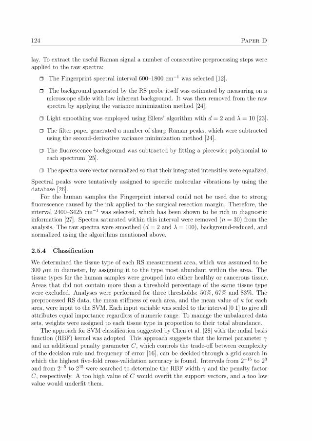
124 Paper D
lay. To extract the useful Raman signal a number of consecutive preprocessing steps wereapplied to the raw spectra:
r The Fingerprint spectral interval 600–1800 cm−1 was selected [12].
r The background generated by the RS probe itself was estimated by measuring on amicroscope slide with low inherent background. It was then removed from the rawspectra by applying the variance minimization method [24].
r Light smoothing was employed using Eilers’ algorithm with d = 2 and λ = 10 [23].
r The filter paper generated a number of sharp Raman peaks, which were subtractedusing the second-derivative variance minimization method [24].
r The fluorescence background was subtracted by fitting a piecewise polynomial toeach spectrum [25].
r The spectra were vector normalized so that their integrated intensities were equalized.
Spectral peaks were tentatively assigned to specific molecular vibrations by using thedatabase [26].
For the human samples the Fingerprint interval could not be used due to strongfluorescence caused by the ink applied to the surgical resection margin. Therefore, theinterval 2400–3425 cm−1 was selected, which has been shown to be rich in diagnosticinformation [27]. Spectra saturated within this interval were removed (n = 30) from theanalysis. The raw spectra were smoothed (d = 2 and λ = 100), background-reduced, andnormalized using the algorithms mentioned above.
2.5.4 Classification
We determined the tissue type of each RS measurement area, which was assumed to be300 µm in diameter, by assigning it to the type most abundant within the area. Thetissue types for the human samples were grouped into either healthy or cancerous tissue.Areas that did not contain more than a threshold percentage of the same tissue typewere excluded. Analyses were performed for three thresholds: 50%, 67% and 83%. Thepreprocessed RS data, the mean stiffness of each area, and the mean value of κ for eacharea, were input to the SVM. Each input variable was scaled to the interval [0 1] to give allattributes equal importance regardless of numeric range. To manage the unbalanced datasets, weights were assigned to each tissue type in proportion to their total abundance.
The approach for SVM classification suggested by Chen et al. [28] with the radial basisfunction (RBF) kernel was adopted. This approach suggests that the kernel parameter γand an additional penalty parameter C, which controls the trade-off between complexityof the decision rule and frequency of error [16], can be decided through a grid search inwhich the highest five-fold cross-validation accuracy is found. Intervals from 2−15 to 23
and from 2−5 to 215 were searched to determine the RBF width γ and the penalty factorC, respectively. A too high value of C would overfit the support vectors, and a too lowvalue would underfit them.

3. Results 125
2.5.5 Statistics
The Lillie test was used to evaluate data normality. The Kruskal-Wallis nonparametrictest followed by the Tukey-Kramer multiple comparison test were used to assess significantdifferences in stiffness and κ values between the tissue types. A p-value less than 0.05was considered statistically significant.
3 Results
The data analysis was conducted on all three human samples and 14 of the 21 porcinesamples. Seven had to be excluded for the following reasons: to avoid damage to the MTS,due to tissue adsorption on the MTS tip, or due to an inappropriate MTS driving frequency.For three samples the measurement area could not be identified on the histologic image.
3.1 SHM
The calibration measurements on gelatin showed that the stiffness indicator was linearto E (R2 ≥ 0.99). Figure 2 shows a typical example of an elasticity mapping. Tissuestructures were clearly observed as differences in their elasticity (Figure 2(c)), wherestroma corresponded to high elasticity regions and lumen mostly to low elasticity regions.
For the porcine samples the median values of E and κ for epithelium, lumen andstroma were significantly different (p < 0.05). There were relatively large overlaps ofthe ranges of E and κ for the tissue types (Figures 3 and 4). The stiffness data was notnormally distributed (p < 0.05), a positive skewness was observed. κ did not follow anormal distribution.
For the human samples there were significant differences between the median E and κvalues (p < 0.05). Lumen was significantly softer than all other groups, except for healthyepithelium (p < 0.05). Prostate stones were significantly stiffer than cancerous epithelium,healthy stroma, and lumen (p < 0.05). The median κ value for cancerous stroma wassignificantly higher than all other groups, except for prostate stones. Furthermore, κwas higher for cancerous epithelium than lumen and healthy epithelium (p < 0.05). Themedian values of E and κ are shown in Figure 5. There were large overlaps between thegroups. E and κ were generally not normally distributed within the groups.
3.2 RS
The mean spectra of the porcine tissue types showed the following differences (Figure 6):
r Changes in the collagen content seen in peaks at 1654 cm−1 (Amide I), 1448 cm−1
(Amide III), 935 cm−1 and 813 cm−1. Stroma showed the highest collagen contentand lumen the lowest.
r Changes in the DNA content seen in the region 640–850 cm−1. Stroma showed thehighest DNA content and lumen the lowest.

126 Paper D
E(kPa)
(c) Stiffness(b) Histologic analysis(a) Histology image
40
60
80
100
120
140
Figure 2: In the histologic analysis lumen is black, epithelium gray and stroma white. The scalebars show 500 µm.
E(kPa)
epithelium (n = 7964) lumen (n = 351) stroma (n = 4577)
0
20
40
60
80
100
120
140
160
180
200
Figure 3: A box plot of the E values for the different porcine tissue types. The line in the middleof the box shows the median, and the bottom and the top of the box show the 25th and 75thpercentile, respectively. The whiskers extend to 1.5 times the interquartile range away from thetop or bottom of the box, or to the furthest observations from the box. Data points outside thewhiskers are plotted individually.

3. Results 127
κ(H
zµm
−2)
epithelium (n = 7964) lumen (n = 351) stroma (n = 4577)
−0.4
−0.2
0
0.2
0.4
0.6
Figure 4: A box plot of the κ values for the different porcine tissue types. The line in the middleof the box shows the median, and the bottom and the top of the box show the 25th and 75thpercentile, respectively. The whiskers extend to 1.5 times the interquartile range away from thetop or bottom of the box, or to the furthest observations from the box. Data points outside thewhiskers are plotted individually.
r Changes in the lipid and fat content seen in the peaks between 1720 to 1790 cm−1.Lumen showed the highest content.
For the human samples it was found that the blue ink applied to the surgical resectionmargin, which is standard clinical procedure, caused a very strong fluorescent signalthat often saturated the CCD detector and swamped the signal from the tissue in theFingerprint interval (Figure 7). However, the fluorescence decreased towards the highwavenumber region.
3.3 Classification
Table 1 shows the classification results for porcine tissue, and Table 2 shows the resultsfor human tissue. The cross-validation accuracy was generally increased for the morehomogeneous tissue regions. Furthermore, by adding RS to SHM the accuracy wassubstantially increased. The values of C and γ ranged from 1.1 to 19000 and 0.023 to 4.8,respectively, for porcine samples. For human tissue C was between 50 and 33000, and γwas between 0.0013 and 8.0.

128 Paper D
(n=7)(n=202)(n=256)(n=1666)(n=93)(n=35)
κ
E
κ(H
zµm
−2)
E(kPa)
stcscesle−0.1
0
0.1
0.2
0
50
100
150
Figure 5: The medians of the E and κ values for the human tissue types. e = epithelium,l = lumen, s = stroma, ce = cancerous epithelium, cs = cancerous stroma, and st = prostatestones.
Table 1: SVM classification accuracies for determining porcine tissue types from SHM and RSdata. CVA = cross-validation accuracy, PA = prediction accuracy.
Homogeneity threshold > 50% (n=1221) > 67% (n=926) > 83% (n=519)CVA PA CVA PA CVA PA
SHM 65.3 65.2 69.5 69.8 82.3 84.6SHM and RS 80.3 100 83.5 99.6 87.3 98.1
Table 2: SVM classification accuracies for distinguishing healthy and cancerous human prostatetissue. CVA = cross-validation accuracy, PA = prediction accuracy.
Homogeneity threshold > 50% (n=204) > 67% (n=190) > 83% (n=178)CVA PA CVA PA CVA PA
SHM 70.1 71.6 68.4 71.6 66.9 72.5SHM and RS 73.0 100 73.7 100 77.0 98.9

3. Results 129
intensity
(arb)
Raman shift (cm−1)
1654
1448935850813606
stroma−lumen
stroma (n = 280)
lumen (n = 41)
epithelium (n = 900)
600 800 1000 1200 1400 1600 1800
Figure 6: The mean Raman spectra of the porcine tissue types. A difference spectrum betweenstroma and lumen, which differed the most, is shown at the top. Its intensity has been multipliedby four to enhance the differences. arb = arbitrary units.

130 Paper Dintensity
(arb)
Raman shift (cm−1)
porcine
human
500 1000 1500 2000 2500 3000
Figure 7: The mean untreated spectra of all human and porcine measurements, showing themagnitude of the ink-induced fluorescence in the human samples. arb = arbitrary units.
4 Discussion
In this study SVM was applied to classify porcine and human prostate tissue from SHMand RS measurements. The combined classification accuracy was 80–87% for healthyporcine tissue, and 73–77% for healthy and cancerous human tissue, depending on thehomogeneity of the tissue. We have shown that the classification accuracy for usingSHM alone is good, and by adding RS to SHM the classification accuracy is substantiallyincreased.
This study confirms the results of Jalkanen et al. [29, 30] and Eklund et al. [31].They concluded that healthy stroma was stiffer than glandular tissue, i.e. lumen andepithelium, and that prostate stones increased tissue stiffness. Furthermore, Jalkanenet al. [29] showed that cancerous prostate tissue was significantly stiffer than glandulartissue (p < 0.05), whereas stroma and prostate stones could not be distinguished fromcancer. This agrees well with our findings, which in addition indicate that cancerousepithelium and healthy stroma are the most difficult tissue types to distinguish, whereascancerous stroma shows increased stiffness (Figure 5). Tuxhorn et al. [32] observed anelevated amount of collagen and loss of smooth muscle in cancerous stroma, which isa possible explanation for the increased stiffness observed in this study. Using SHM,Murayama et al. [11] mapped the elasticity of human prostate and observed that thecancerous node (about 100 µm in diameter) was stiffer than surrounding normal tissues.However, it was technically difficult to compare the elasticity map to the histology image.Thus, the elasticity distribution could not be further analyzed [11].

4. Discussion 131
In this study, the localization of the measurement area on the histology images wasdone manually. The histology specimens were often deformed, which made it more difficultto overlap the morphological features of the histologic images and the stiffness maps. Sincethe step size of the SHM mappings was merely 50 µm, a slight localization error wouldhave caused many measurement points to be misclassified. To minimize the impact ofthis, we conducted the analysis of SHM data on homogeneous tissue regions. We observedthat the separation of E for the tissue types then increased, and the deviations fromnormality decreased. This confirmed that many points had been misclassified. For theSVM analysis the measurement areas were 300 µm in diameter, so the localization errorsdid not affect the outcome as much. Still, higher classification accuracy may have beenattained with smaller localization errors. In future studies an objective and more accuratelocalization may be provided by developing an algorithm that can assist in identifyingthe measurement area.
Histology specimens from both above and below the measurement sample were acquiredto give a rough estimate of the tissue distribution across the sample. The specimensthat were cut below the measurement samples were of low quality. We were only able toconclude that the cancerous tissue to some extent continued across the human 500-µmsections. Thus, the histologic analysis conveyed information only about the tissue type atthe topmost layer of the tissue. The probes picked up signal from deep-laying layers oftissue. The Raman spectra even contained peaks from the filter paper under the tissue.Jalkanen et al. [29] showed that the TRM was sensitive to layers of tissue lying deeperthan the impression depth in a weighted tissue proportion model. In this study, it cantherefore be suspected that since the MTS was impressed about 40 µm, it also sensedeven deeper layers.
Maintaining tissue moistness is fundamental for SHM measurements [10, 33]. Inthis study we used a simple but effective method in which the sample was placed on afilter paper and surrounded by a shelter to which a constant flow of PBS was supplied.Extensive tests were carried out to find an optimal amount of flow to prevent tissuedehydration during the total SHM measurement time of approx. 30 minutes. Six repeatedSHM mappings were acquired on the same area of 10 × 10 points on porcine prostatetissue during 30 minutes. The optimal flow was determined by minimizing the change inmean stiffness while maximizing the correlation coefficients between the maps. In thefinal SHM mappings no general trend of sample dehydration was observed in plots ofE versus acquisition time. However, dehydration/flooding may have contributed to thelarge spread of E. In future studies the stability of the mappings and the quality of thedata may be enhanced by using a moisture chamber, or immersing the sample fully inPBS [10].
Gelatin was chosen as material for stiffness calibration because it is a biologicalmaterial easily prepared in a stiffness range comparable to that of prostate tissue. Apotential disadvantage of gelatin is that its stiffness is temperature dependent. Thiseffect was suppressed by storing the samples in a refrigerator and minimizing the timein room temperature to less than three minutes. No temperature effect was observed inthe SHM data. For two of the porcine prostate samples the gelatin calibration from the
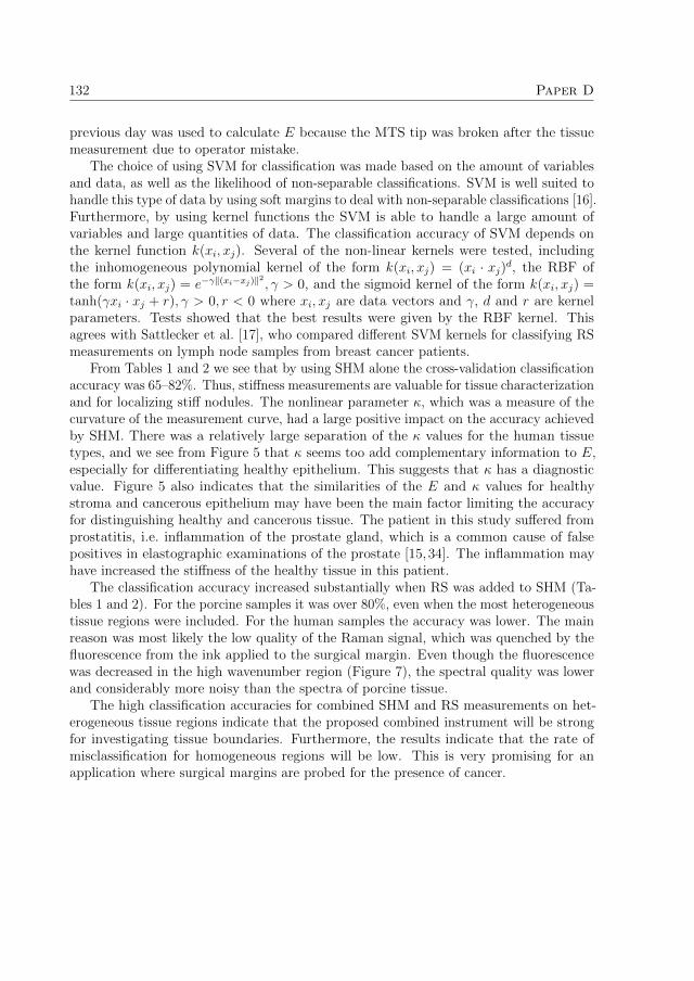
132 Paper D
previous day was used to calculate E because the MTS tip was broken after the tissuemeasurement due to operator mistake.
The choice of using SVM for classification was made based on the amount of variablesand data, as well as the likelihood of non-separable classifications. SVM is well suited tohandle this type of data by using soft margins to deal with non-separable classifications [16].Furthermore, by using kernel functions the SVM is able to handle a large amount ofvariables and large quantities of data. The classification accuracy of SVM depends onthe kernel function k(xi, xj). Several of the non-linear kernels were tested, includingthe inhomogeneous polynomial kernel of the form k(xi, xj) = (xi · xj)d, the RBF ofthe form k(xi, xj) = e−γ‖(xi−xj)‖
2, γ > 0, and the sigmoid kernel of the form k(xi, xj) =
tanh(γxi · xj + r), γ > 0, r < 0 where xi, xj are data vectors and γ, d and r are kernelparameters. Tests showed that the best results were given by the RBF kernel. Thisagrees with Sattlecker et al. [17], who compared different SVM kernels for classifying RSmeasurements on lymph node samples from breast cancer patients.
From Tables 1 and 2 we see that by using SHM alone the cross-validation classificationaccuracy was 65–82%. Thus, stiffness measurements are valuable for tissue characterizationand for localizing stiff nodules. The nonlinear parameter κ, which was a measure of thecurvature of the measurement curve, had a large positive impact on the accuracy achievedby SHM. There was a relatively large separation of the κ values for the human tissuetypes, and we see from Figure 5 that κ seems too add complementary information to E,especially for differentiating healthy epithelium. This suggests that κ has a diagnosticvalue. Figure 5 also indicates that the similarities of the E and κ values for healthystroma and cancerous epithelium may have been the main factor limiting the accuracyfor distinguishing healthy and cancerous tissue. The patient in this study suffered fromprostatitis, i.e. inflammation of the prostate gland, which is a common cause of falsepositives in elastographic examinations of the prostate [15,34]. The inflammation mayhave increased the stiffness of the healthy tissue in this patient.
The classification accuracy increased substantially when RS was added to SHM (Ta-bles 1 and 2). For the porcine samples it was over 80%, even when the most heterogeneoustissue regions were included. For the human samples the accuracy was lower. The mainreason was most likely the low quality of the Raman signal, which was quenched by thefluorescence from the ink applied to the surgical margin. Even though the fluorescencewas decreased in the high wavenumber region (Figure 7), the spectral quality was lowerand considerably more noisy than the spectra of porcine tissue.
The high classification accuracies for combined SHM and RS measurements on het-erogeneous tissue regions indicate that the proposed combined instrument will be strongfor investigating tissue boundaries. Furthermore, the results indicate that the rate ofmisclassification for homogeneous regions will be low. This is very promising for anapplication where surgical margins are probed for the presence of cancer.

5. Conclusion 133
5 Conclusion
The combination of SHM and RS can successfully be used to identify different prostatetissue types by using SVM. The results indicate accurate detection of cancerous prostatetissue. This is promising for the development of an instrument that combines these twomethods for tissue characterization during prostate cancer surgery.
Acknowledgments
This work was supported by grants from the Objective 2 Norra Norrland-EU StructuralFund and the Kempe Foundation. We wish to thank Mats Gustavsson for helpingus obtaining porcine prostate samples, Kerstin Lofquist and Kerstin Stenberg at thedept. of Pathology and Cytology at Sunderby Hospital for preparing porcine histologyspecimens, and Kerstin Almroth, Pernilla Andersson and Birgitta Ekblom at the urologyand pathology units at Norrland’s University Hospital for preparing human histologyspecimens.
References
[1] B. Tareen, J. Kimmel, and W. C. Huang, “Contemporary treatment of high-risklocalized prostate cancer”, Expert Rev Anticancer Ther, vol. 10, pp. 1069–1076, 2010.
[2] T. H. V. der Kwast, M. Bolla, H. V. Poppel, P. V. Cangh, K. Vekemans, L. D.Pozzo, J.-F. Bosset, K. H. Kurth, F. H. Schroder, and L. Collette, “Identification ofpatients with prostate cancer who benefit from immediate postoperative radiotherapy:EORTC 22911”, J Clin Oncol, vol. 25, pp. 4178–4186, 2007.
[3] O. Yossepowitch, A. Bjartell, J. A. Eastham, M. Graefen, B. D. Guillonneau, P. I.Karakiewicz, R. Montironi, and F. Montorsi, “Positive surgical margins in radicalprostatectomy: outlining the problem and its long-term consequences”, Eur Urol,vol. 55, pp. 87–99, 2009.
[4] S. Candefjord, K. Ramser, and O. A. Lindahl, “Technologies for localization anddiagnosis of prostate cancer”, J Med Eng Technol, vol. 33, pp. 585–603, 2009.
[5] S. Candefjord, M. Nyberg, V. Jalkanen, K. Ramser, and O. A. Lindahl, “Combin-ing fibre optic Raman spectroscopy and tactile resonance measurement for tissuecharacterization”, Meas Sci Technol, vol. 21, 125801 (8 pp.), 2010.
[6] O. A. Lindahl, C. E. Constantinou, A. Eklund, Y. Murayama, P. Hallberg, andS. Omata, “Tactile resonance sensors in medicine”, J Med Eng Technol, vol. 33,pp. 263–273, 2009.
[7] Y. Murayama and S. Omata, “Fabrication of micro tactile sensor for the measurementof micro-scale local elasticity”, Sensor Actuat A, vol. 109, pp. 202–207, 2004.

134 Paper D
[8] Y. Murayama, C. Constantinou, and S. Omata, “Development of Tactile Mappingsystem for the stiffness characterization of tissue slice using novel tactile sensingtechnology”, Sensor Actuat A, vol. 120, pp. 543–549, 2005.
[9] T. Oie, H. Suzuki, T. Fukuda, Y. Murayama, S. Omata, K. Kanda, and Y. Nakayama,“Tactile Mapping System: A Novel Imaging Technology for Surface Topography andElasticity of Tissues or Organs”, Innovations, vol. 4, pp. 345–350, 2009.
[10] T. Oie, H. Suzuki, Y. Murayama, T. Fukuda, S. Omata, K. Kanda, K. Takamizawa,and Y. Nakayama, “Surface elasticity imaging of vascular tissues in a liquid envi-ronment by a scanning haptic microscope”, J Artif Organs, vol. 13, pp. 121–125,2010.
[11] Y. Murayama, S. Omata, T. Yajima, Q. Peng, K. Shishido, D. M. Peehl, and C. E.Constantinou, “High Resolution Regional Elasticity Mapping of the Human Prostate”,in Proceedings of the 29th Annual International Conference of the IEEE EMBS. CiteInternationale, Lyon, France. August 23-26, 2007, pp. 5802–5805, 2007.
[12] A. Mahadevan-Jansen and R. R. Richards-Kortum, “Raman spectroscopy for thedetection of cancers and precancers”, J Biomed Opt, vol. 1, pp. 31–70, 1996.
[13] A. Nijssen, S. Koljenovic, T. C. B. Schut, P. J. Caspers, and G. J. Puppels, “Towardsoncological application of Raman spectroscopy”, J Biophotonics, vol. 2, pp. 29–36,2009.
[14] P. Matousek, “Deep non-invasive Raman spectroscopy of living tissue and powders”,Chem Soc Rev, vol. 36, pp. 1292–1304, 2007.
[15] S. Candefjord, K. Ramser, and O. A. Lindahl, “Effects of snap-freezing and near-infrared laser illumination on porcine prostate tissue as measured by Raman spectro-scopy”, Analyst, vol. 134, pp. 1815–1821, 2009.
[16] C. Cortes and V. Vapnik, “Support-Vector Networks”, Machine Learning, vol. 20,pp. 273–297, 1995.
[17] M. Sattlecker, C. Bessant, J. Smith, and N. Stone, “Investigation of support vectormachines and Raman spectroscopy for lymph node diagnostics”, Analyst, vol. 135,pp. 895–901, 2010.
[18] Y. Murayama, C. Constantinou, and S. Omata, “Micro-mechanical sensing plat-form for the characterization of the elastic properties of the ovum via uniaxialmeasurement”, J Biomech, vol. 37, pp. 67–72, 2004.
[19] I. N. Sneddon, “The relation between load and penetration in the axisymmetricboussinesq problem for a punch of arbitrary profile”, Int J Eng Sci, vol. 3, pp. 47–57,1965.

References 135
[20] Y. Hattori, Y. Komachi, T. Asakura, T. Shimosegawa, G.-I. Kanai, H. Tashiro, andH. Sato, “In vivo Raman study of the living rat esophagus and stomach using amicro-Raman probe under an endoscope”, Appl Spectrosc, vol. 61, pp. 579–584, 2007.
[21] Y. Komachi, T. Katagiri, H. Sato, and H. Tashiro, “Improvement and analysis of amicro Raman probe”, Appl Opt, vol. 48, pp. 1683–1696, 2009.
[22] C.-C. Chang and C.-J. Lin, LIBSVM: a library for support vector machines, 2001.Software available at http://www.csie.ntu.edu.tw/~cjlin/libsvm.
[23] P. H. Eilers, “A perfect smoother”, Anal Chem, vol. 75, pp. 3631–3636, 2003.
[24] Y. L. Loethen, D. Zhang, R. N. Favors, S. B. G. Basiaga, and D. Ben-Amotz,“Second-derivative variance minimization method for automated spectral subtraction”,Appl Spectrosc, vol. 58, pp. 272–278, 2004.
[25] A. Cao, A. K. Pandya, G. K. Serhatkulu, R. E. Weber, H. Dai, J. S. Thakur, V. M.Naik, R. Naik, G. W. Auner, R. Rabah, and D. C. Freeman, “A robust methodfor automated background subtraction of tissue fluorescence”, J Raman Spectrosc,vol. 38, pp. 1199–1205, 2007.
[26] Z. Movasaghi, S. Rehman, and I. Rehman, “Raman spectroscopy of biological tissues”,Appl Spectrosc Rev, vol. 42, pp. 493–541, 2007.
[27] S. Koljenovic, T. C. B. Schut, R. Wolthuis, B. de Jong, L. Santos, P. J. Caspers,J. M. Kros, and G. J. Puppels, “Tissue characterization using high wave numberRaman spectroscopy”, J Biomed Opt, vol. 10, 031116 (11 pp.), 2005.
[28] Y.-W. Chen and C.-J. Lin, “Combining SVMs with Various Feature SelectionStrategies”, in Feature Extraction (I. Guyon, M. Nikravesh, S. Gunn, and L. Zadeh,eds.), vol. 207 of Studies in Fuzziness and Soft Computing, pp. 315–324, SpringerBerlin / Heidelberg, 2006.
[29] V. Jalkanen, B. M. Andersson, A. Bergh, B. Ljungberg, and O. A. Lindahl, “Res-onance sensor measurements of stiffness variations in prostate tissue in vitro – aweighted tissue proportion model”, Physiol Meas, vol. 27, pp. 1373–1386, 2006.
[30] V. Jalkanen, B. M. Andersson, A. Bergh, B. Ljungberg, and O. A. Lindahl, “Prostatetissue stiffness as measured with a resonance sensor system: a study on silicone andhuman prostate tissue in vitro”, Med Biol Eng Comput, vol. 44, pp. 593–603, 2006.
[31] A. Eklund, A. Bergh, and O. A. Lindahl, “A catheter tactile sensor for measuringhardness of soft tissue: measurement in a silicone model and in an in vitro humanprostate model”, Med Biol Eng Comput, vol. 37, pp. 618–624, 1999.
[32] J. A. Tuxhorn, G. E. Ayala, M. J. Smith, V. C. Smith, T. D. Dang, and D. R. Rowley,“Reactive stroma in human prostate cancer: induction of myofibroblast phenotypeand extracellular matrix remodeling”, Clin Cancer Res, vol. 8, pp. 2912–2923, 2002.

136 Paper D
[33] T. Oie, Y. Murayama, T. Fukuda, C. Nagai, S. Omata, K. Kanda, H. Yaku, andY. Nakayama, “Local elasticity imaging of vascular tissues using a tactile mappingsystem”, J Artif Organs, vol. 12, pp. 40–46, 2009.
[34] L. Pallwein, M. Mitterberger, G. Pinggera, F. Aigner, F. Pedross, J. Gradl, A. Pelzer,G. Bartsch, and F. Frauscher, “Sonoelastography of the prostate: comparison withsystematic biopsy findings in 492 patients”, Eur J Radiol, vol. 65, pp. 304–310, 2008.