Geophys. J. Int. (0000) 000, 000–000

Combined mechanical and melting damage model for1

geomaterials2

Jie Liu1,∗, Ali Karrech2, Klaus Regenauer-Lieb1,3,∗∗

1 Laboratory for Multiscale Earth System Dynamics and Geothermal Research, School of Earth and Environment,

The University of Western Australia, M004, 35 Stirling Hwy, Crawley, WA 6009, Australia

2 The University of Western Australia, School of Civil and Resource Engineering, M051, 35 Stirling Hwy, Crawley, WA 6009, Australia

3 CSIRO Earth Science and Resource Engineering, 26 Dick Perry Ave., Kensington, WA 6151, Australia

∗ Now at the School of Earth Science and Geological Engineering, also at Supercomputing Institute, Sun Yat-sen University,

135 West Xingang Road, Guangzhou, 510275, China

∗∗ Now at the School of Petroleum Engineering, University of New South Wales, NSW 2052, Australia

3

9 May 20144

SUMMARY5

We present a new damage model combining mechanics and partial6

melting in accordance with the principles of non-equilibrium ther-7

modynamics. On the mechanical side, elasto-viscoplactic damage is8

considered based on a self-consistent far from equilibrium thermo-9

dynamic framework; on the melt side, partial melting is calculated10

by using the thermodynamic MELTS Gibbs energy minimiser. In this11

framework the partial melt appears as an additional damage parameter.12

The numerical implementations are accomplished by using Abaqus13

solver and the extendable User Material Subroutine (UMAT). A sim-14

plified continental extension model is used to test the approach. This15

new model can be applied to geodynamic problems involving brittle16

and ductile faulting, partial melting, magma generation, and the inter-17

action between these activities.18

2 J. Liu et al.

Key words: elasto-viscoplastic damage, partial melting, geodynam-19

ics, numerical modeling20

1 INTRODUCTION21

Mechanical damage models based on energetic consideration have matured over their recent history (Chaboche(1987);22

Houlsby & Puzrin(2000); Houlsby & Puzrin(2006)). Recently, a model for pressure and temperature sensitive ge-23

omaterials has been developed (Karrech et al.(2011a)Karrech, Regenauer-Lieb, & Poulet; Karrech et al.(2011b)Karrech,24

Regenauer-Lieb, & Poulet) which was specifically formulated for geodynamic problems involving lithosphere in25

depth. For rocks at elevated temperature, partial melt provide another damage mechanism to considerably weaken26

the rock matrix and form localised deformation processes. However, the combined effects of mechanical damage27

and melting damage have not yet been explored. This problem is of great significance for geodynamics as partial28

melt are expected to interact with the shear zones at the base of the lithosphere in regions where the temperature29

and pressure conditions can cause partial melting. A good example are mid-ocean ridges where melt extraction30

form the oceanic crust during sea floor spreading. Continental rift systems are another example where magmatism31

and normal faulting interacts with melts at the base of the lithosphere (Turcotte & Schubert(2002)). In order to be32

able to model the effect of partial melting on lithosphere deformation we extend the earlier lithosphere damage33

work (Karrech et al.(2011a)Karrech, Regenauer-Lieb, & Poulet; Karrech et al.(2011b)Karrech, Regenauer-Lieb,34

& Poulet) to include self-consistent melting relationships via Gibbs energy minimisation and the explicit effect35

of the partial melt on damage of the solid rock matrix.36

A different approch of damage mechanics based on energy consideration has been presented previously fo-37

cussing on different aspects, such as brittle damage (Lyakhovsky et al.(1997)Lyakhovsky, Ben-Zion, & Agnon;38

Hamiel et al.(2004b)Hamiel, Lyakhovsky, & Agnon; Hamiel et al.(2004a)Hamiel, Liu, Lyakhovsky, Ben-Zion,39

& Lockner; Lyakhovsky et al.(2005)Lyakhovsky, Ben-Zion, & Agnon; Nanjo et al.(2005)Nanjo, Turcotte, &40

Shcherbakov), two-phase fluid dynamic approaches considering continuum damage (Ricard et al.(2001)Ricard,41

Bercovici, & Schubert; Ricard & Bercovici(2003); Landuyt & Bercovici(2009)), or ductile fracture and other42

weakening effects (Regenauer-Lieb(1999); Hieronymus(2004)). These models cover a wide range of applica-43

tions using either a solid or a fluid dynamic approach. (Karrech et al.(2011a)Karrech, Regenauer-Lieb, & Poulet)44

proposed a theory of continuum damage that combines the above describe fluid and solid mechanical considera-45

tions particularly relevant for long geological time scales. However, none of these approaches consider explicitly46

the role of melting in the lithosphere.47

As the problem involves heat generation through deformation and heat transfer through conduction, material48

advection, phase transitions and in particular melting a full thermomechanical approach where temperature is49

coupled with displacement is considered here. Early work focussed on the problem of heat generation and shear50

3

localisation. The importance of thermomechanical coupling appearing as shear heating in viscous flows was51

first recognised in the 60’s (Gruntfest(1963)). Thermal mechanical coupling was later on found to be impor-52

tant for instabilities at the lithosphere-asthenosphere boundary(Yuen & Schubert(1977)), ice flows (Schubert &53

Yuen(1982); Yuen et al.(1986)Yuen, Saari, & Schubert), catastrophic landslides (Vardoulakis(2002); Veveakis54

et al.(2007)Veveakis, Vardoulakis, & DiToro.; Goren & Aharonov(2007); Goren et al.(2010)Goren, Aharonov,55

& Anders) and faults (Wibberley & Shimamoto(2005); Rice(2006)). The current work builds on the numerical56

schemes and methods for calculating shear heating instabilities in the lithosphere as well as lithospheric deforma-57

tions presented in further details in (Regenauer-Lieb & Yuen(1998); Regenauer-Lieb & Yuen(2003); Regenauer-58

Lieb & Yuen(2004)).59

The theoretical and numerical thermo-mechanical modeling framework is easily extended to include melting60

and damage, as damage is interpreted as an intensive variable that accounts for the sensitivity of the elastic61

properties. The evolution of damage, conversely, is described by the dissipation potential that is operating in62

the inelastic regime. The approach also can include pressure dependent non-associated deformation (Karrech63

et al.(2011b)Karrech, Regenauer-Lieb, & Poulet) which in their melt-absent models was important to communi-64

cate the pure shear-dominated deformation regime of the lower crust to the deformation regime of the upper crust65

that also includes volume changes. This aspect is particularly important for the consideration of melting at the66

base of the lithosphere as again volumetric deformation may play a role through the volume changes induced by67

melting and fluid transport.68

Partial melting of rocks occurs when temperature exceeds the liquidus of at least one mineral. Generally, it hap-69

pens in the environment of the upper mantle and under hot environment in the lower crust. Three factors affect70

partial melting: 1) temperature, higher temperature above the liquidus cause higher degrees of partial melting; 2)71

composition, different minerals have different liquidus and are in turn affected by the water content; 3) pressure,72

decrease of pressure favours partial melting. When condition for melting are first met, melt accumulates on the73

grain boundary and softens the rock matrix. Several mechanisms can be envisioned that depend on the chemistry74

and the dihedral angle. The most pronounced weakening effect can occur under net tensile stresses and grain75

boundary wetting where the matrix support is lost and the fluid behaviour governs the response of the system.76

We do not consider in this work stress condition for pure tensile failure as these are only likely to occur at the77

surface of the Earth. Our model is specifically designed for bulk compressive effective stresses as the increasing78

overburden in the lithosphere and mantle is expected to cause an effective compressive stress regime. This implies79

in other words that the solid rock matrix govern the mechanical behaviour. In the present work we only solve this80

mechanical problem of the effect of melting on deformation and do not solve the melt transport problem.81

Partial melting has been studied in both laboratory experiments and by theoretical thermodynamic considera-82

tions. Experimental studies (Mysen & Kushiro(1977); Fujii & Scarfe(1985); Kinzler & Grove(1992); Falloon83

4 J. Liu et al.

et al.(1999)Falloon, Green, Danyushevsky, & Faul) provide essential understanding of the occurrence of partial84

melting but are limited to specific compositions, temperature and pressure conditions. In order to generalise a85

computation formulation for partial melting for a range of temperatures, pressures and compositions, compu-86

tational methods need to be adopted. Early studies (Klein & Langmuir(1987); McKenzie & Bickle(1988); Niu87

& Batiza(1991); Langmuir et al.(1992)Langmuir, Klein, & Plank) used results from experiments to parame-88

terise the extent of melting as functions of temperature, composition and pressure based on simplified thermody-89

namic relationships. These empirical relationship are not fully robust beyond the range of temperature, compo-90

sition and pressure of experiments available. Therefore, a new approach was developed (Ghiorso & Sack(1995);91

Hirschmann et al.(1998)Hirschmann, Ghiorso, Wasylenki, Asimow, & Stolper) which follows thermodynamic92

principles and calculates the phase equilibria of partially molten rocks by minimising the Gibbs or Helmholtz93

free energy. The computational package MELTS is the most widely used platform for such thermodynamic cal-94

culations in igneous system, particularly for mantle compositions. The basic MELTS can compute equilibrium95

phase relations over the temperature range 500 - 2000 ◦C and the pressure range 0 - 2 GPa. For the condi-96

tions of higher temperatures and pressures, suitable packages are available in extension of the MELTS family of97

codes, such as pMELTS, xMELTS and mdMELTS (http://melts.ofm-research.org/). pMELTS is frequently used98

for lithosphere models where pressure is above 2 GPa (with depth more than 70 km) and temperature within 250099

◦C. xMELTS and mdMELTS are generally not used for solid lithosphere models.100

This thermodynamic approach allows a direct implementation into the damage mechanics formalism as both are101

based on solving for the basic energy functions. These are the rate of Helmholtz (Gibbs) free energy produc-102

tion/release in equilibrium with the dissipation potential. Therefore, partial melting can be easily incorporated103

into a mechanical damage model, where the extent of the partial melting is calculated using (p)MELTS. The104

amount of melting appears therefore as a new damage mechanism where the solid matrix is weakened by the de-105

gree of partial melting. This weakening comprises both elastic and viscoplastic damage effects in the Helmholtz106

free energy (elastic) and the dissipation potentials (viscoplastic) (Karrech et al.(2011a)Karrech, Regenauer-Lieb,107

& Poulet; Karrech et al.(2011b)Karrech, Regenauer-Lieb, & Poulet). As all the factors are considered in the108

unified thermodynamic framework, the model can be applied to geodynamic problems involving brittle and duc-109

tile faulting, partial melting, magma generation and the interaction between different damage mechanisms. In110

this contribution we focus on the presentation of the basic theory and the numerical implementations. We also111

illustrate the resulting triple-damage formulation on a simple large-scale lithosphere extension model.112

5

2 GOVERNING EQUATIONS113

2.1 Helmholtz free energy and the generalised stresses of thermodynamics114

The model introduced in this paper extends the formulation of geomaterials with coupled brittle/ductile thermo-115

mechanical damage through the incorporation of melting damage. We call this brittle-ductile-melt damage a triple116

damage model. We extend the Helmholtz free energy for coupled brittle/ductile damage (Karrech et al.(2011a)Karrech,117

Regenauer-Lieb, & Poulet; Karrech et al.(2011b)Karrech, Regenauer-Lieb, & Poulet), by the specific Helmholtz118

free energy ψ from the melting damage including latent heat effects:119

ρψ(εij , ε

inij , T,D, ϕm

)= (1−D)Gεeijε

eij +

1

2[(1− φm)(1−D)λe + φmλ

em] (εekk)2

−3 [(1− φm)(1−D)Kα+ φmKmαm] εekk(T − T0)

− [(1− φm)c+ φmcm](T − T0)2

2T0+ Lφm

(1)120

where ρ is the material density, εij is the total strain tensor, εinij is the inelastic strain tensor, and εeij = εij − εinij121

is the elastic strain tensor, T is temperature and T0 is a reference temperature, D is the mechanical damage122

parameter of solid part, ϕm is the melt fraction by volume, G is the shear modulus of solid, λe and λem are the123

first Lame’s constant of solid and melt respectively, K and Km are bulk modulus for solid and melt respectively,124

α and αm are the coefficient of thermal expansion of solid and melt respectively, c and cm are the specific heat125

capacity of solid and melt respectively.126

The quadratic term in temperature follows from allowing the consideration of deformation on the value of the127

heat capacity. This correction term accounts for the variation of heat capacity with temperature (Houlsby &128

Puzrin(2000)).129

Since we do not solve the equations for melt transfer in our damage mechanics solver we limit the matrix weak-130

ening from partial melting to an arbitrary value of 25% melt which is much lower than the other damage mech-131

anisms. Another reason for limiting the melting damage fraction is our assumed linear energy superposition of132

the solid and melt phases. This underestimates the weakening for large melt fractions but is acceptable for small133

fractions. We therefore, present a conservative estimate of the mechanical effects of the melt generation.134

The derivative of Helmholtz specific free energy with respect to time t is135

ρ∂ψ

∂t= ρ

∂ψ

∂εeij: εeij + ρ

∂ψ

∂TT + ρ

∂ψ

∂DD + ρ

∂ψ

∂ϕmϕm. (2)136

Using the first and second laws of thermodynamics, we have137

ρ∂ψ

∂εeij= σij

= 2(1−D)Gεeij + [(1− φm)(1−D)λe + φmλem] εekkδij

+3 [(1− φm)(1−D)Kα+ φmKmαm] (T − T0) δij

(3)138

ρ∂ψ

∂D= YD = −Gεeijεeij −

1

2(1− φm)λe (εekk)2 + 3 [(1− φm)Kα] εekk (4)139

6 J. Liu et al.

ρ∂ψ

∂ϕm= Ym

=1

2[λe

m − (1−D)λe] (εekk)2

−3 [Kmαm − (1−D)Kα] (T − T0)εekk

− (cm − c)(T − T0)2

2T0+ L

(5)140

The volume strain εekk can be expressed by the defomred volume and original volume values. Thus Eq. (5) can141

be written as:142

Ym =1

2[λe

m − (1−D)λe](V − V0

V0

)2

−3 [Kmαm − (1−D)Kα] (T − T0)(V − V0

V0

)− (cm − c)

(T − T0)2

2T0+ L

(6)143

2.2 Dissipation function and thermodynamic velocities144

The intrinsic dissipation function (rate) for this problem can be written as145

D = σij εinij + YDD + Ymϕm, (7)146

where the dissipations of inelastic deformation (the first term of right-hand-side), mechanical damage (the second147

term), and melt damage (the third term) are considered respectively.148

The principle of maximum entropy production requires that if the dissipative forces σij , YD , Ym are prescribed,149

the actual velocities εinij , D, ϕm must maximise the dissipation D subject to the side conditions150

σij εinij ≥ 0, YDD ≥ 0, and Ymϕm ≥ 0. (8)151

Based on this principle, the flow rules, or the thermodynamic velocities εinij , D, ϕm of Eq. (8) can be introduced152

by using Legendre-Fenchel transformation (Fenchel(1949); Rockafellar(1996)).153

For visco-plastic behavior, a yield function (elasticity envelope) f1 (σij) − k1(εinij)

= 0 are generally defined154

based on experiments and plastic criteria. For mechanical damage and melting damage, two similar envelope155

f2 (YD)− k2 (D) = 0 and f3 (Ym)− k3 (ϕm) = 0 can be defined. In this study we use a generalised potential156

of the form Φ = f1 (σij) + f2(YD) + f3(Ym) such that the flow rules of the thress processes read:157

εinij = λ∂f1∂σij

, D = λ∂f2∂YD

, ϕm = λ∂f3∂Ym

.158

By maximizing the dissipation under the equality constraints of the envelopes, Karrech et al. (Karrech et al.(2011a)Karrech,159

Regenauer-Lieb, & Poulet; Karrech et al.(2011b)Karrech, Regenauer-Lieb, & Poulet) have given the flow rules160

of visco-plasticity as161

εinij = λ∂f1∂σij

= λ

(3

2

sijσeq

+ rβδij

), (9)162

where sij is the deviatoric stress, σeq =√

32sijsij , rβ can be interpreted as the effect of the pressure dependent163

dilatation; and the flow rules of mechanical damage follow as164

7

D = λ∂f2∂YD

= λ

[1

(1−D)n+1+N (YD)− 1

], (10)165

where n is the exponent of the dislocation creep mechanism, N (YD) =(YDH

)Kdescribes the nucleation of166

mechanical damage, here H and K are material constants. The additional flow rule of melting damage in this167

paper will be determined from the results of computations of MELTS as f3 (Ym) and k3 (ϕm) are not well168

defined. For the specific composition in the analysed model, melting is dependent on temperature and pressure,169

while pressure is a linear function of volume, thus the flow rule can be expressed as:170

ϕm = λ∂f3∂Ym

= λ(∂f3∂T

∂T

∂Ym+∂f3∂V

∂V

∂Ym

), (11)171

where ∂f3∂T

represents the variation of the melting envelop versus temperature, and ∂f3∂V

represents the variation172

of the melting function versus volume. Both of them can be determined by fitting the results of MELTS that173

describe the areas of melting (see the following section). ∂T∂Ym

and ∂V∂Ym

are reciprocals of the derivatives of Ym174

with respect to T and volume V , respectively. Thus, the flow rule of melting can be written as:175

ϕm = λ

(A

1∂Ym∂T

+B1

∂Ym∂V

)= λ

(A

E+B

F

), (12)176

whereA = ∂f3∂T

andB = ∂f3∂V

can be fitted from the results of MELTS for specific rock composition as mentioned177

above, and178

E =∂Ym

∂T= 3 [(1−D)Kα−Kmαm]

V − V0

V0+ (c− cm)

T − T0

T0,179

F =∂Ym

∂V= [− (1−D)λe + λe

m]V − V0

V0+ 3 [(1−D)Kα−Kmαm] (T − T0).180

These two formulae are related to volume (pressure), temperature, mechanical damage portion, and some material181

parameters, thus the flow rule of melting is determined when A and B are known.182

3 NUMERICAL IMPLEMENTATIONS183

We use the finite element method, in particular, the implicit code Abaqus/Standard to implement the approach184

numerically. Abaqus provides flexibility to integrate the material response in User Material Subroutines (UMAT).185

We use this capability rather than the numerical descriptions provided by the Abaqus library. Therefore we use186

only the Abaqus matrix solver and write our own Fortran code to implement the above theory in a finite el-187

ement discrete time domain. Details of the numerical implementations are found in Karrech et al. (Karrech188

et al.(2011b)Karrech, Regenauer-Lieb, & Poulet). Our Fortran subroutine simply extends the formalism by a189

third damage mechanism. Here we briefly discuss how the extension for this additional melting damage is imple-190

mented.191

(i) Obtaining parameters from the input file or from a computation of previous step, including melting fraction.192

In the initial step, melting damage ϕm is assigned based on the temperature distribution and pressure state of the193

model.194

8 J. Liu et al.

(ii) Prediction correction scheme of stress – this step is very similar to the description in (Karrech et al.(2011b)Karrech,195

Regenauer-Lieb, & Poulet) but melting fraction ϕm is involved. In particular, a trial solution of stress of an in-196

crement is197

σ∗ = σ0 + (1−D) (1− ϕm)Cijkl∆εkl − 3 (1−D) (1− ϕm)Kα∆Tδij198

+ϕmCmijkl∆εkl − 3ϕmKmαm∆Tδij .199

(iii) Consistent tangent modulus – the difference between this study with the previous work (Karrech et al.(2011b)Karrech,200

Regenauer-Lieb, & Poulet) is that the incremental relationship of stress and strain is expressed as201

∆(σij)n+1 = (1−D)(1− ϕm)(C−1ijkl + ∆λ1Mijkl)

−1(∆εkl −∆λ1Nij).202

(iv) Additional computation of the flow rule of melting in Eq. (11) from material parameters and the results203

from (p)MELTS. This is accomplished by a new Fortran function and the computation is straightforward.204

(v) Modifying the melting damage from the consistency factor and the flow rule calculated in step iv). The205

new melting damage is saved as a state variable and used in the next time increment as input parameters.206

Readers with further interest in the numerical formulation can refer to Section 3 of Karrech et al. (Karrech207

et al.(2011b)Karrech, Regenauer-Lieb, & Poulet) for details .208

4 MELTING DAMAGE FROM (P)MELTS209

In the calculation of melting flow rule ϕm, two coefficients A = ∂f3∂T

and B = ∂f3∂V

are obtained from the results210

of (p)MELTS.211

The basic MELTS (Ghiorso & Sack(1995); Ghiorso et al.(2002)Ghiorso, Hirschmann, Reiners, & Kress) is cal-212

ibrated on a wide variety of bulk compositions in the mafic system and it works especially well for MORBS213

and alkalic mafic magmas. It is not suitable for lithospheric conditions over 2 GPa of pressure and 2000 ◦C of214

temperature. Alternatively, for these conditions we can use pMELTS, which is suitable for the temperature range215

of 1000 - 2500 ◦C and pressure range of 1 - 4 GPa (Ghiorso et al.(2002)Ghiorso, Hirschmann, Reiners, & Kress).216

pMELTS is a revised calibration of MELTS from an extended experimental database and is optimized for mantle-217

like bulk compositions at near solidus conditions (0 - 30 % melting). The temperature and pressure ranges are218

recommended, slightly beyond the ranges would be allowed, but much below or above the ranges may cause the219

failure of the model. Phase equilibria involving hornblende and biotite are at present difficult to model with the220

MELTS package, and consequently simulating the evolution of intermediate to silica-rich calc-alkaline systems221

is not recommended (Ghiorso & Sack(1995); Asimow & Ghiorso(1998)).222

The (p)MELTS can consider scenarios for magmatic processes as a function of :223

(i) temperature and pressure (Gibbs energy minimization),224

9

(ii) temperature and volume (Helmholtz energy minimization),225

(iii) enthalpy and pressure (entropy maximization)226

(iv) entropy and pressure (enthalpy minimization).227

Isenthalpic (constant enthalpy), isentropic (constant entropy) or isochoric (constant volume) scenarios can be228

utilised to explore magmatic processes such as energy constrained assimilation, adiabatic decompression melting,229

or post-entrapment crystallisation in phenocryst melt inclusions. Optionally, equilibrium can be computed in230

systems open to oxygen transfer at fixed chemical potential (fugacity) of oxygen. This allows both equilibrium231

and fractional crystallisration of magmas to be modeled along a specified oxygen buffer.232

Therefore using (p)MELTS we can calculate the thermodynamic properties of the melts of an initial chemical233

composition corresponding to for the specific geodynamic problem being analysed. (p)MELTS outputs compo-234

sitions of solid and liquid, and thermodynamic data at different temperature and pressure. Among the thermo-235

dynamic data, temperature, pressure, the fraction of melt, and volume are what we interest. Here we present an236

example to demonstrate the procedure from (p)MELTS output to Abaqus input data. The example is also used in237

the geodynamic models in the next section to verify the algorithms and numerical implementations of the effect238

of melting damage.239

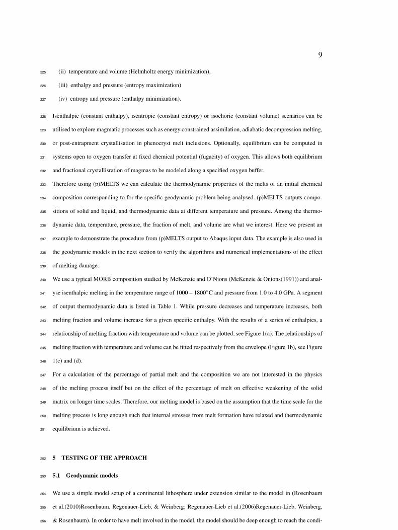
We use a typical MORB composition studied by McKenzie and O’Nions (McKenzie & Onions(1991)) and anal-240

yse isenthalpic melting in the temperature range of 1000 – 1800◦C and pressure from 1.0 to 4.0 GPa. A segment241

of output thermodynamic data is listed in Table 1. While pressure decreases and temperature increases, both242

melting fraction and volume increase for a given specific enthalpy. With the results of a series of enthalpies, a243

relationship of melting fraction with temperature and volume can be plotted, see Figure 1(a). The relationships of244

melting fraction with temperature and volume can be fitted respectively from the envelope (Figure 1b), see Figure245

1(c) and (d).246

For a calculation of the percentage of partial melt and the composition we are not interested in the physics247

of the melting process itself but on the effect of the percentage of melt on effective weakening of the solid248

matrix on longer time scales. Therefore, our melting model is based on the assumption that the time scale for the249

melting process is long enough such that internal stresses from melt formation have relaxed and thermodynamic250

equilibrium is achieved.251

5 TESTING OF THE APPROACH252

5.1 Geodynamic models253

We use a simple model setup of a continental lithosphere under extension similar to the model in (Rosenbaum254

et al.(2010)Rosenbaum, Regenauer-Lieb, & Weinberg; Regenauer-Lieb et al.(2006)Regenauer-Lieb, Weinberg,255

& Rosenbaum). In order to have melt involved in the model, the model should be deep enough to reach the condi-256

10 J. Liu et al.

Table 1. A segment of output of thermodynamic data of pMELTS.

P T F phi S H V Cp mass fO2 rhol rhos viscosity

10000 1673.15 0.1656 0.1847 265.97 -1.25E+6 32.41 134.86 100.78 -8.31 2.79 3.18 1.26

12000 1656.83 0.0840 0.0943 262.10 -1.25E+6 31.90 131.93 100.78 -8.82 2.81 3.20 1.24

14000 1634.43 0.0236 0.0272 258.26 -1.25E+6 31.52 129.52 100.78 -10.51 2.77 3.21 1.43

16000 1597.03 0.0067 0.0080 254.37 -1.25E+6 31.31 128.46 100.78 -12.59 2.70 3.22 1.76

18000 1554.81 0.0020 0.0025 250.41 -1.25E+6 31.17 127.74 100.78 -13.19 2.62 3.23 3.09

20000 1510.57 0.0014 0.0017 246.35 -1.25E+6 31.05 127.13 100.78 -12.78 2.63 3.25 3.58

22000 1465.85 0.0012 0.0015 242.18 -1.25E+6 30.94 126.51 100.78 -12.39 2.66 3.26 3.78

24000 1421.70 0.0011 0.0014 237.90 -1.25E+6 30.79 125.83 100.78 -11.73 2.70 3.27 3.89

26000 1378.13 0.0011 0.0013 233.52 -1.25E+6 30.63 125.09 100.78 -10.81 2.73 3.29 3.93

28000 1333.78 0.0010 0.0012 229.01 -1.25E+6 30.49 124.38 100.78 -10.06 2.77 3.31 3.95

30000 1288.85 0.0010 0.0012 224.37 -1.25E+6 30.36 123.67 100.78 -9.36 2.81 3.32 3.92

P – pressure (bar), T – temperature (K), F – melt fraction by mass, phi – melt fraction by volume, S – system entropy (J/K), H

– system enthalpy (J), V – volume (cm3), Cp – heat capacity (J/K), fO2 – system oxygen fugacity in log10, rhol – density of

liquid (g/cm3), rhos – density of bulk solid (g/cm3), and viscosity – viscosity of the liquid in log10 (poise).

1271  1363  

1441  1515  

1570  1642  

1730  0.00  

0.05  

0.10  

0.15  

0.20  

0.25  

0.30  

30.7   30.9   31.1   31.2   31.4   31.6  32.1   32.8  

T  

Melt  frac+on  

V  

0.25-­‐0.30  0.20-­‐0.25  0.15-­‐0.20  0.10-­‐0.15  0.05-­‐0.10  0.00-­‐0.05  

1270  

1401  1532  

1664  0.00  

0.05  

0.10  

0.15  

0.20  

0.25  

0.30  

30.6  30.9   31.3   31.6   31.9   32.2   32.5   32.8  

33.2  

Melt  frac+on  

T  V  

0.25-­‐0.30  0.20-­‐0.25  0.15-­‐0.20  0.10-­‐0.15  0.05-­‐0.10  0.00-­‐0.05  

φm  =  0.0012*T  -­‐  1.79  

0.00  

0.05  

0.10  

0.15  

0.20  

0.25  

0.30  

1300   1400   1500   1600   1700   1800  

Melt  frac+on

 

Temperature  (K)  

φm  =  0.1517*V  -­‐  4.75  

0.00  

0.05  

0.10  

0.15  

0.20  

0.25  

0.30  

30   30.5   31   31.5   32   32.5   33   33.5  

Melt  frac+on

 

Volume  (cm3)  

(a)   (b)  

(c)   (d)  

Fig.  1.  Mel>ng  frac>on  and  the  rela>onships  with  temperature  and  volume.  (a)  Results  of  (p)MELTS  of  constant  enthalpy  (isenthalpic);  (b)  Smoothed  surface  of  mel>ng  frac>on  from  the  results  of  (a);  (c)  fiRng  the  rela>onship  between  mel>ng  frac>on  and  temperature,  mel>ng  starts  from  1495K;  (d)  fiRng  the  rela>on  ship  between  mel>ng  frac>on  and  volume,  mel>ng  starts  from  31.3  cm3  (of  100  g  composi>on).  Note  large  circles  in  (c)  and  (d)  are  points  used  in  fiRng  the  rela>onships  

Figure 1. Melting fraction and the relationships with temperature and volume. (a) Results of (p)MELTS of constant enthalpy

(isenthalpic); (b) Smoothed surface of melting fraction from the results of (a); (c) fitting the relationship between melting

fraction and temperature, melting starts from 1495K; (d) fitting the relation ship between melting fraction and volume, melting

starts from 31.3 cm3 (of 100 g composition). Note large circles in (c) and (d) are points used in fitting the relationships.

11

Free  slip  

Free  boundary  Quartz  

Olivine  

Fig.  2.  Model  setup.  (a)  Three-­‐layer  structure  and  boundary  condi?ons,  extensional  velocity  12.7  mm/yr  each  side  ;  (b)  ini?al  temperature  distribu?on  with  random  perturba?on  of  Model  1.  

(a)  

Feldspar  

0  

(b)  

200  

0  

160  L/km  

Figure 2. Model setup. (a) Three-layer structure and boundary conditions, extensional velocity of 4.0×10−11 m/s (12.7 mm/yr)

each side ; (b) initial temperature distribution with random perturbation.

tions for melting. Thus the 2D plane-strain model is extended to 160 km depth and the numerical domain is 200257

km wide at initial conditions (Figure 2a). It consists of a horizontally stratified rheology of three layers: 1) quartz,258

20 km in thickness, 2) feldspar, below the quartz layer, 10 km in thickness, 3) olivine, below the feldspar layer,259

130 km in thickness. The model is discretised by 76,832 rectangular elements. The initial element size is 510 m260

width and 816 m depth. In order to avoid remeshing during extension we have chosen initial element shapes that261

on average will go through a 1x1 aspect ratio in the middle of the extension process. The top boundary of the262

model is a free surface while the bottom boundary is free slip in x direction and pinned in y. We are considering an263

extensional model on the side boundaries symmetric boundary conditions. The extension velocity of 4.0×10−11264

m/s (12.7 mm/yr) is applied to the both sides of the model.265

266

The model rheology and parameters were described in the Appendix of (Rosenbaum et al.(2010)Rosenbaum,267

Regenauer-Lieb, & Weinberg; Regenauer-Lieb et al.(2006)Regenauer-Lieb, Weinberg, & Rosenbaum). We also268

refer to the damage rheology described in (Karrech et al.(2011a)Karrech, Regenauer-Lieb, & Poulet; Karrech269

et al.(2011b)Karrech, Regenauer-Lieb, & Poulet). Additional parameters for melting phase are taken from (Ryan(1980))270

and (Bass(1995)). The major parameters are summarised in Table 2. Three different values of elastic modulus for271

melt are used in our model to test the effects.272

We consider a basic thermal model controlled by the following ingredients. The heat flow at the bottom of the273

lithosphere is assumed to be 20 mW/m2 and the exponentially decaying radiogenic heat contribution to the top274

10 km of the crust has a total contribution of 30 mW/m2 corresponding to the analytical solution of the steady275

state 50 mW/m2 surface heat flow continental lithosphere (Turcotte & Schubert(2002)). We give the temperature276

on the top boundary to be 290 K and from the thermal model it is 1628.94 K on the bottom boundary. Randomly277

distributed temperature perturbation is considered. The initial temperature distribution is shown in Figure 2b.278

12 J. Liu et al.

Table 2. Parameters used in the numerical model.

Parameter [unit] Quartz Feldspar Olivine

Shear heating efficiency 0.9

Density [Kg/m−3] 2700 2800 3300

Young’s modulus - solid [Pa] 5.0×1010 6.5×1010 8.0×1010

Young’s modulus - melt [Pa] 4.5×1010 (test-1)

5.0×109 (test-2)

5.0×108 (test-3)

6.0×1010 (test-1)

6.5×109 (test-2)

6.5×108 (test-3)

7.5×1010 (test-1)

8.0×109 (test-2)

8.0×108 (test-3)

Poisson ratio 0.3 (solid); 0.45 (melt)

Thermal expansion [K−1] 3.1×10−5

Specific heat [J/(kg*K)] 4.0×105

Thermal conductivity [W/(mK)] 2.5 (solid)

1.5 (melt)

2.5 (solid)

1.5 (melt)

3.2 (solid)

2.0 (melt)

Pre-exponential parameter [Pa−ns−1] 3.98×10−21 7.94×10−26 6.31×10−12

Power-law exponent 2.6 3.1 4.0

Activation enthalpy [kJ/mol] 134.0 163.0 135.0

Yield stress at low/high pressure [Pa] 5×108 (low); 8×107 (high)

279

In addition to the model in Fig. 2, we also use a submodel to show an extra example and test the sensitivity280

of mesh resolution. The submodel is in the scale of 80 km deep and 100 km wide, with the similar stratified281

layers of quartz (20 km), feldspar (10 km), and olivine (50 km). Similar thermal structure of Fig. 2b is used in282

the submodel but with two significant differences: 1) the temperature on the top boundary is given to be 850 K283

and it is 1653.54 K on the bottom boundary. This is because the model of 80 km deep cannot reach the condition284

for melting if using a realistic temperature of the surface of the crust. 2) the pertubation of temperature is not285

considered in this submodel. A notch of 8.16 km wide and 20.41 km deep is set in the centre of the top boundary.286

The material of the notch is simple Drucker-Prager plasticity with elastic modulus 2.0 GPa, yield stress 10 MPa287

and the angle of friction 30◦, and damage is not considered inside the notch. Other materials have the same pa-288

rameters as in Table 2. We descrete the model to two mesh resolutions. The normal mesh is with the resolution289

of 510 m by 816 m, the same to the mesh used in the model of Fig.2. The fine mesh is with the resolution of 255290

m by 408 m. All the boundary conditions are exactly the same as the model in Fig. 2.291

13

5.2 Results292

Figure 3 shows the mechanical damage of the model of Fig. 2 in test-1 after the extension of 12.80 kyr (a), 19.81293

kyr (c), 20.19 kyr (d), and 55.77 kyr (e), as well as the partial melting damage at 12.80 kyr (b) and 55.77 kyr294

(f). Here the elastic moduli of melt are slightly lower than those of solid materails. Comparing Figure 3 (a) and295

(b), we see that the mechanical damage initially forms in the layer above the partial melting layer. Upon further296

deformation it propagates both downwards and upwards. The propagation of these localised damage areas is very297

fast at the beginning period of their development. As the temperature field does not change very much in the298

model, the melting layer stays in an almost stationary state. However, the two zoomed in images in panel (f) show299

that the top boundary of the partial melting layer is dislocated by the two main faults as the development of the300

mechanical damage. This demonstrates the interaction of mechanical damage and partial melting damage.301

Upon further deformation we notice in Figure 3(c)-(e) that the mechanical damage zones have entered into the302

melting layer and reached the bottom boundary. The maximum melting fraction is close to 15% in the model,303

which happens in areas of high temperature perturbation. For most areas of the melting, the melting fraction is304

8%. The predicted mechanical damage zones in the melt layer could be identified in geological field observations305

as faults propagating through a partially molten rock. In such observations faults are often interpreted as discrete306

pathways for melt extraction pumping melts into the shallower part of the lithosphere and providing access to the307

surface of the crust. Our current model does not consider this scenario and only focuses on thermal-mechanical308

deformation.309

Figure 4 shows the mechanical damage of the model of Fig. 2 in test-2, where the elastic moduli of melt are310

one order lower than those of the solid materials. In this formulation we can see that all of the lower part of the311

model has developed mechanical damage based on the mechanical damage criteria. In the shallow part, faults are312

developing upwards in a fast sequence. The distribution of faults is different from Figure 3, but intrinsically, the313

patterns are similar.314

In test-3 the elastic moduli of melt are two orders lower than those of solid materials. The results are very similar315

to those of test-2 and show almost the same distribution and development of faults. Although the shallow part316

of the model creates almost the same faulting structure, the deep part of the model has different deformation for317

test-2 and test-3, see Figure 5. Inelastic deformations of test-2 (Figure 5a) and test-3 (Figure 5b) have the same318

legend. We see that the only difference is the slightly higher inelastic deformation in the deep part of the model319

of test-3 over test-2.320

We proceed by testing the results of the mesh resolution studies performed in our earlier contributions on litho-321

sphere damage (Karrech et al.(2011a)Karrech, Regenauer-Lieb, & Poulet) and shear heating models (Regenauer-322

Lieb & Yuen(2004)). Our damage mechanics approach does not introduce an additional material length scale and323

is solely regularised by the thermal-mechanical solution to the heat problem. A steady state shear zone devel-324

14 J. Liu et al.

ops when the width of the heat conduction away from the shear zone equates the shear heating in the shear zone.325

Therefore, the shear zone has a square root relationship of width with the thermal diffusivity (order of 10−6m2/s)326

times the characteristic time (order 1012s). This leads to a width of the shear zone of the order of kilometres and327

a mesh size requirement of the order of 100 meters (Regenauer-Lieb & Yuen(2004)). Fig. 6 tests the mesh res-328

olution requirements formulated for the lithosphere deformation problem (Regenauer-Lieb & Yuen(2004)) in a329

submodel with a central notch subject to symmetric extension. Fig. 6a shows the initial temperature of the model.330

Note that there is no perturbation of temperature and the minimum temperature at the top boundary is 850 K.331

Fig. 6b to Fig. 6f are results of the model after 0.36 Ma extension with a speed of 12.7 mm/yr. Fig. 6b shows the332

corresponding melt damage. Fig. 6c to Fig. 6f compare the mechanical damage results computed from a coarse333

mesh (c and e) and fine mesh (d and f) of the whole submodel (c and d). Figures e and f compare the zoom334

in. As expected the coarse mesh which is just below the resolution limit required by the mesh resolution study335

(Regenauer-Lieb & Yuen(2004)) shows a number of artefacts such as the development of an asymmetric solution336

for symmetric boundary conditions. This artefact is removed when the mesh size is refined to a few hundred337

meters.338

As the model and boundary conditions are all symmetric, the perfectly symmetric deformation showed in the fine339

mesh computation is more reasonable and reliable than the coarse mesh, demonstrating the high accuracy of the340

fine mesh. The existance of the notch affects the pattern of the faults in this model. More information and detailed341

analysis about the effect of notch will be discussed in a follow up paper (Regenauer-Lieb et al.(2014)Regenauer-342

Lieb, Rosenbaum, Lyakhovsky, Liu, Weinberg, Segev, & Weinstein).343

344

6 CONCLUSION345

This paper presents a new theoretical approach to incorporate melting into a continuum thermodynamic dam-346

age formalism and describes its numerical implementation. The approach is designed for describing the effect of347

melting on the dynamics of continental deformation. This approach is an extension of the damage visco-plasticity348

model for pressure and temperature sensitive geomaterials of Karrech et al. (Karrech et al.(2011a)Karrech,349

Regenauer-Lieb, & Poulet; Karrech et al.(2011b)Karrech, Regenauer-Lieb, & Poulet). Partial melting is embed-350

ded in the governing equations as an extra damage component. The initial melting and the evolution of melting351

with temperature and pressure are analysed by using (p)MELTS, using the method of minimising the Helmholtz352

free energy to derive energetically self-consistent melting models. As the mechanical damage and melt damage353

are both developed within the thermodynamic framework, the combination of the two components is natural and354

the theoretical deduction is consolidated.355

The numerical implementations are fulfilled by using the User Material Subroutine (UMAT) of Abaqus and the356

15

(a)   (b)  

(c)   (d)  

(e)   (f)  

1.0  

0.8  

0.6  

0.4  

0.2  

0.0  

Mech.  Dam.  8.0%  

6.4%  

4.8%  

3.2%  

1.6%  

0.0%  

Melt  Dam.  0  

160  0   200  L/km  

0  

160  0   200  L/km  

Figure 3. Mechanical damage of test-1 after the extension of 12.80 kyr (a), 19.81 kyr (c), 20.19 kyr (d), and 55.77 kyr (e), and

partial melting damage at 12.80 kyr (b) and 55.77 kyr (f). Panels of mechanical damage and melting damage have consistent

legends, respectively.

subroutine is upgraded from the version of Karrech et al. (Karrech et al.(2011b)Karrech, Regenauer-Lieb, &357

Poulet). Since the implementation is essentially an extension of the previous work the numerical procedure was358

found to be robust.359

A continental extension models is used to test the approach. The model demonstrates that mechanical damage360

starts from the melting layer. The localised shear zone or faults can propagate both upwards and downwards.361

While at shallow level the mechanical damage develops without melting damage, at depth mechanical damage362

and melting form fully coupled pairs. The mechanical damage developed at shallow levels could provide channel363

for the segregation of melt from depth to the surface of crust. This problem is not investigated by our current364

formulation.365

16 J. Liu et al.

(a)   (b)  

(c)   (d)  

0.95  

0.76  

0.57  

0.39  

0.29  

0.00  

Mech.  Dam.  

0  

160  0   200  L/km  

0  

160  

0  

160  

0  

160  0   200  L/km  

0   200  L/km   0   200  L/km  

Figure 4. Mechanical damage of test-2 after the extension of 230.26 kyr (a), 235.19 kyr (b), 244.70 kyr (c), and 294.15 kyr (d)

In this paper we have focussed on the introduction of a new model combining mechanical damage and melting366

damage. As all principal factors affecting lithospheric deformation can now be considered in the unified thermo-367

dynamic framework, the model can be applied to solve fundamental geodynamic problems involving brittle and368

ductile faulting, partial melting, magma generation and the fully coupled interaction between these damage mech-369

anisms. We focus on the theoretical deduction and technical presentation here, an application of the approach to370

solve the problem alkaline intraplate volcanism in extensional tectonic setting is in preparation (Regenauer-Lieb371

et al.(2014)Regenauer-Lieb, Rosenbaum, Lyakhovsky, Liu, Weinberg, Segev, & Weinstein).372

(a)   (b)  

0.35  

0.28  

0.21  

0.14  

0.07  

0.00  

Inelas.  Def.  0  

160  0   200  L/km  

0  

160  0   200  L/km  

Figure 5. Inelastic deformation of test-2 (a) and test-3 (b) after the extension of 312 kyr.

17

Notch  

(a)   (b)  

(c)   (d)  

(e)   (f)  

0  

80  0   100  L/km  

0  

80  

0  

80  

0  

80  

0   100  L/km  

0   100  L/km   0   100  L/km  

Figure 6. Smaller testing model and the results of difference mesh resolutions. (a) Initial temperature; (b) melt damage (same

for coarse and fine mesh); (c) mechanical damage with coarse mesh; (d) mechanical damage of fine mesh; (e) local area

indicated by the rectangle in (c) with quilt plot; (f) local area indicated by the rectangle in (d) . Results in (b) to (f) are all after

the extension of 0.36 Ma.

ACKNOWLEDGMENTS373

This study was supported by Australia Research Council through project DP1094050.374

REFERENCES375

Asimow, P. D. & Ghiorso, M. S., 1998. Algorithmic modifications extending melts to calculate subsolidus phase relations,376

American Mineralogist, 83, 1127–1131.377

Bass, J. D., 1995. Elasticity of minerals, glasses, and melts, in Mineral Physics and Crystallography A Hand Book of Physical378

Constants, American Geophysical Union.379

18 J. Liu et al.

Chaboche, J. L., 1987. Continuum damage mechanics - present state and future-trends, Nuclear Engineering and Design,380

105(1), 19–33.381

Falloon, T. J., Green, D. H., Danyushevsky, L. V., & Faul, U. H., 1999. Peridotite melting at 1.0 and 1.5 gpa: an experimental382

evaluation of techniques using diamond aggregates and mineral mixes for determination of near-solidus melts, Journal of383

Petrology, 40(9), 1343–1375.384

Fenchel, W., 1949. On conjugate convex functions, Canadian Journal of Mathematics, 1, 73–77.385

Fujii, T. & Scarfe, C. M., 1985. Composition of liquids coexisting with spinel lherzolite at 10-kbar and the genesis of morbs,386

Contributions to Mineralogy and Petrology, 90(1), 18–28.387

Ghiorso, M. S. & Sack, R. O., 1995. Chemical mass transfer in magmatic processes. iv. a revised and internally consistent388

thermodynamic model for the interpolation and extrapolation of liquid-solid equilibria in magmatic systems at elevated389

temperatures and pressures, Contributions to Mineralogy and Petrology, 119, 197–212.390

Ghiorso, M. S., Hirschmann, M. M., Reiners, P. W., & Kress, V. C. I., 2002. The pmelts: An revision of melts aimed at improving391

calculation of phase relations and major element partitioning involved in partial melting of the mantle at pressures up to 3392

gpa, Geochemistry, Geophysics, Geosystems, 3(5).393

Goren, L. & Aharonov, E., 2007. Long runout landslides: The role of frictional heating and hydraulic diffusivity., Geophys.394

Res. Lett., 34, L07301.395

Goren, L., Aharonov, E., & Anders, M. H., 2010. The long runout of the heart mountain landslide:heating, pressurization, and396

carbonate decomposition, J. Geophys. Res., 115, B10210.397

Gruntfest, I., 1963. Thermal feedback in liquid flow: Plane shear at constant stress., Trans. Soc. Rheol., 7, 95–207.398

Hamiel, Y., Liu, Y. F., Lyakhovsky, V., Ben-Zion, Y., & Lockner, D., 2004a. A viscoelastic damage model with applications to399

stable and unstable fracturing, Geophysical Journal International, 159(3), 1155–1165.400

Hamiel, Y., Lyakhovsky, V., & Agnon, A., 2004b. Coupled evolution of damage and porosity in poroelastic media: theory and401

applications to deformation of porous rocks, Geophysical Journal International, 156(3), 701–713.402

Hieronymus, C. F., 2004. Control on seafloor spreading geometries by stress- and strain-induced lithospheric weakening, Earth403

and Planetary Science Letters, 222(1), 177–189.404

Hirschmann, M. M., Ghiorso, S., Wasylenki, L. E., Asimow, P. D., & Stolper, E. M., 1998. Calculation of peridotite partial405

melting from thermodynamic models of minerals and melts. i. review of methods and comparison with experiments, Journal406

of Petrology, 39(6), 1091–1115.407

Houlsby, G. T. & Puzrin, A. M., 2000. A thermomechanical framework for constitutive models for rate-independent dissipative408

materials, International Journal of Plasticity, 16(9), 1017–1047.409

Houlsby, G. T. & Puzrin, A. M., 2006. Principles of hyperplasticity: An approach to plasticity theory based on thermodynamic410

principles, Springer-Verlag.411

Karrech, A., Regenauer-Lieb, K., & Poulet, T., 2011a. Continuum damage mechanics for the lithosphere, Journal of Geophys-412

ical Research - Solid Earth, 116(B04205).413

Karrech, A., Regenauer-Lieb, K., & Poulet, T., 2011b. A damaged visco-plasticity model for pressure and temperature sensitive414

geomaterials, International Journal of Engineering Science, 49(10), 1141–1150.415

Kinzler, R. J. & Grove, T. L., 1992. Primary magmas of midocean ridge basalts .1. experiments and methods, Journal of416

Geophysical Research - Solid Earth, 97(B5), 6885–6906.417

Klein, E. M. & Langmuir, C. H., 1987. Global correlations of ocean ridge basalt chemistry with axial depth and crustal418

thickness, Journal of Geophysical Research - Solid Earth, 92(8), 8089–8115.419

19

Landuyt, W. & Bercovici, D., 2009. Formation and structure of lithospheric shear zones with damage, Physics of the Earth and420

Planetary Interiors, 175(3-4), 115–126.421

Langmuir, C. H., Klein, E. M., & Plank, T., 1992. Petrological systematics of midocean ridge basalts - constraints on melt422

generation beneath ocean ridges, in Mantle Flow and Melt Generation at Mid-Ocean Ridges, vol. 71, pp. 183–280, eds423

Morgan, J., Blackman, D., & Sinton, J., American Geophysical Union.424

Lyakhovsky, V., Ben-Zion, Y., & Agnon, A., 1997. Distributed damage, faulting, and friction, Journal of Geophysical Research425

- Solid Earth, 102(B12), 27635–27649.426

Lyakhovsky, V., Ben-Zion, Y., & Agnon, A., 2005. A viscoelastic damage rheology and rate- and state-dependent friction,427

Geophysical Journal International, 161(1), 179–190.428

McKenzie, D. & Bickle, M. J., 1988. The volume and composition of melt generated by extension of the lithosphere, Journal429

of Petrology, 29(3), 625–679.430

McKenzie, D. & Onions, R. K., 1991. Partial melt distributions from inversion of rare-earth element concentrations, Journal of431

Petrology, 32(5), 1021–1091.432

Mysen, B. O. & Kushiro, I., 1977. Compositional variations of coexisting phases with degree of melting of peridotite in upper433

mantle, American Mineralogist, 62(9-10), 843–856.434

Nanjo, K. Z., Turcotte, D. L., & Shcherbakov, R., 2005. A model of damage mechanics for the deformation of the continental435

crust, Journal of Geophysical Research - Solid Earth, 110(B07403).436

Niu, Y. L. & Batiza, R., 1991. An empirical-method for calculating melt compositions produced beneath midocean ridges437

- application for axis and off-axis (seamounts) melting, Journal of Geophysical Research - Solid Earth, 96(13), 21753–438

21777.439

Regenauer-Lieb, K., 1999. Dilatant plasticity applied to alpine collision: ductile void growth in the intraplate area beneath the440

eifel volcanic field, Journal of Geodynamics, 27, 1–21.441

Regenauer-Lieb, K. & Yuen, D., 1998. Rapid conversion of elastic energy into shear heating during incipient necking of the442

lithosphere, Geophysical Research Letters, 25(14), 2737–2740.443

Regenauer-Lieb, K. & Yuen, D., 2003. Modelling shear zones in geological and planetary sciences: solid- and fluid-thermal-444

mechanical approaches, Earth Sci. Rev., 63, 295–349.445

Regenauer-Lieb, K. & Yuen, D., 2004. Positive feedback of interacting ductile faults from coupling of equation of state,446

rheology and thermal-mechanics, Physics of Earth and Planetary Interiors, 142(1-2), 113–135.447

Regenauer-Lieb, K., Weinberg, R. F., & Rosenbaum, G., 2006. The effect of energy feedbacks on continental strength, Nature,448

442(7098), 67–70.449

Regenauer-Lieb, K., Rosenbaum, G., Lyakhovsky, V., Liu, J., Weinberg, R., Segev, A., & Weinstein, Y., 2014. Melt instabil-450

ities in cold lithosphere and implications for volcanism in the azraq-sirhan graben, Gepphysical Journal International, in451

preparation.452

Ricard, Y. & Bercovici, D., 2003. Two-phase damage theory and crustal rock failure: the theoretical ’void’ limit, and the453

prediction of experimental data, Geophysical Journal International, 155(3), 1057–1064.454

Ricard, Y., Bercovici, D., & Schubert, G., 2001. A two-phase model for compaction and damage 2. applications to compaction,455

deformation, and the role of interfacial surface tension, Journal of Geophysical Research - Solid Earth, 106(B5), 8907–456

8924.457

Rice, J. R., 2006. Heating and weakening of faults during earthquake slip, J. Geophys. Res., 111, B05311.458

Rockafellar, R. T., 1996. Convex Analysis, Princeton University Press.459

20 J. Liu et al.

Rosenbaum, G., Regenauer-Lieb, K., & Weinberg, R., 2010. Interaction between mantle and crustal detachments: A nonlinear460

system controlling lithospheric extension, Journal of Geophysical Research - Solid Earth, 115(B11412).461

Ryan, M. P., 1980. Mechanical behaviour of magma reservoir envelopes: Elasticity of olivine tholeiite solidus, Bulletin of462

Volcanology, 43(4), 743–772.463

Schubert, G. & Yuen, D., 1982. Initiation of ice ages by creep instability and surging of the east antarctic ice sheet, Nature,464

296, 127–130.465

Turcotte, D. L. & Schubert, G., 2002. Geodynamics, Cambridge University Press.466

Vardoulakis, I., 2002. Dynamic thermo-poro-mechanical analysis of catastrophic landslides., Geotechnique, 52, 157–171.467

Veveakis, E., Vardoulakis, I., & DiToro., G., 2007. Thermoporomechanics of creeping landslides: The 1963 vaiont slide,468

northern italy., J. Geophys. Res., 112, F03026.469

Wibberley, C. & Shimamoto, T., 2005. Earthquake slip weakening and asperities explained by thermal pressurization., Nature,470

426(4), 689–692.471

Yuen, D. & Schubert, G., 1977. Asthenospheric shear flow: thermally stable or unstable?, Geophys. Res. Lett, 4(11), 503–506.472

Yuen, D., Saari, M., & Schubert, G., 1986. Explosive growth of shear-heating instabilities in the down-slope creep of ice sheets,473

J. Glaciology, 32(112), 314–320.474