College Enrollment Trends and Pattern Evaluation

College Enrollment Trends and Pattern Evaluation

“A Data Analytics Investigation”

by

Aishwary Pawar

A thesis submitted in partial fulfillment

of the requirements for the degree of

Master of Science in Engineering

(Industrial and Systems Engineering)

in the University of Michigan-Dearborn

2020

Master’s Thesis Committee:

Assistant Professor DeLean Tolbert, Chair

Associate Professor Gengxin Li

Assistant Professor Abdallah Chehade

Lecturer IV Claudia Walters

ii

Acknowledgements

First and foremost, I would like to express my sincere gratitude to my advisor Dr. DeLean Tolbert

for giving me an excellent opportunity to work and explore the area of Engineering Education, for

the continuous support, motivation, and guidance throughout my master’s program. Besides my

advisor, I would like to extend my sincere thanks to the rest of my thesis committee: Dr. Claudia

Walters, Dr. Abdallah Chehade, and Dr. Gengxin Li, for their encouragement and insightful

comments. I’m incredibly grateful to Dr. Gengxin Li for helping me with the analysis work.

Finally, I must express my very profound gratitude to my parents Krishnakant and Aruna for

providing me with unfailing support throughout my education. I would also like to thank my friend

Priya for her constant support.

iii

Table of Contents

Acknowledgements ......................................................................................................................... ii

List of Tables ................................................................................................................................ VI

List of Figures .............................................................................................................................. VII

Abstract ...................................................................................................................................... VIII

Chapter 1. Introduction ............................................................................................................. 1

Chapter 2. Review of the Literature ......................................................................................... 3

2.1 Undergraduate Enrollment, Retention and Graduation at a Public University ............... 3

2.2 Pre-Existing Research on Factors Affecting Undergraduate Enrollment, Retention,

Graduation and Dropout ............................................................................................................. 4

2.2.1 Distance (Proximity) ................................................................................................... 6

2.2.2 Race and Ethnicity ...................................................................................................... 7

2.2.3 Gender ......................................................................................................................... 8

2.2.4 Internet ...................................................................................................................... 10

2.2.5 Income- (Household Income and Neighborhoods Poverty Level) ........................... 13

2.2.6 Scholarships/ Pell Eligibility..................................................................................... 14

2.2.6.a Effects on Enrollment ....................................................................................... 14

2.2.6.b Effects on Retention .......................................................................................... 15

Chapter 3. Purpose of Study ................................................................................................... 17

iv

Chapter 4. Proposed Research Question................................................................................. 19

Chapter 5. Methodology ......................................................................................................... 20

5.1 Feature Selection ........................................................................................................... 22

5.1.1 GLM- Negative Binomial Regression ...................................................................... 23

5.1.1.a Multicollinearity ............................................................................................... 24

5.1.1.b Variance Inflation Factor (VIF) ........................................................................ 25

5.1.2 Lasso Regression ...................................................................................................... 26

5.2 Data Visualization Using QGIS .................................................................................... 27

5.3 Spearmen Correlation Analysis .................................................................................... 28

5.4 Cluster Analysis ............................................................................................................ 29

5.5 Control Group Analysis ................................................................................................ 31

Chapter 6. Results ................................................................................................................... 33

6.1 Feature Selection ........................................................................................................... 33

6.1.1 GLM- Negative Binomial Regression ...................................................................... 33

6.1.2 Lasso Regression ...................................................................................................... 37

6.2 Data Visualization Using QGIS .................................................................................... 39

6.3 Spearmen Correlation Analysis (Linear Association Of Random Variables) .............. 49

6.4 Cluster Analysis ............................................................................................................ 51

6.5 Control Group Analysis ................................................................................................ 57

Chapter 7. Discussion ............................................................................................................. 62

Chapter 8. Conclusion ............................................................................................................ 65

Chapter 9. Future Work .......................................................................................................... 66

v

References ..................................................................................................................................... 68

vi

List of Tables

Table 1 Data distribution .............................................................................................................. 21

Table 2 Methods used ................................................................................................................... 32

Table 3 Negative binomial regression model ............................................................................... 34

Table 4 Initial variance inflation factor (VIF) .............................................................................. 35

Table 5 Final variance inflation factor (VIF) ................................................................................ 36

Table 6 Final regression model ..................................................................................................... 37

Table 7 Lasso regression coefficients ........................................................................................... 38

Table 8 Final selected features ...................................................................................................... 39

Table 9 Spearmen correlation results ............................................................................................ 50

Table 10 Percentage distribution of factors based on clusters ...................................................... 54

Table 11 Mean values for all predictor variables in each cluster ................................................. 54

Table 12 Cluster analysis results................................................................................................... 55

Table 13 Spearman correlation coefficient per cluster ................................................................. 56

Table 14 Control group 1 range .................................................................................................... 58

Table 15 Control group 2 range .................................................................................................... 60

Table 16 Comparison to control group 1 ...................................................................................... 61

Table 17 Comparison to control group 2 ...................................................................................... 61

vii

List of Figures

Figure 1 Estimated model of student persistence (Ethington) ........................................................ 5

Figure 2 Conceptual schema for dropout from college (Tinto, 1975) ............................................ 5

Figure 3 Number persisting to 8th semester (Ohland et al., 2011) ............................................... 10

Figure 4 Regularization parameter (𝜆) .......................................................................................... 38

Figure 5 UM-Dearborn CECS undergraduate enrollment count of year (2015 - 2019) from

respective Zip Codes ..................................................................................................................... 40

Figure 6 Percentage of people with bachelor’s degrees or higher in the respective Zip Codes ... 41

Figure 7 Percentage of people with high school graduation or higher in the respective Zip Codes

in Michigan ................................................................................................................................... 42

Figure 8 Median household income of people in the respective Zip Codes in Michigan ............ 43

Figure 9 Percentage of households with internet access in the respective Zip Codes in Michigan

....................................................................................................................................................... 44

Figure 10 Percentage of minority population in the respective Zip Codes in Michigan .............. 45

Figure 11 Travel distance to UM- Dearborn from the respective Zip Codes ............................... 46

Figure 12 Total population in a Zip Code ..................................................................................... 47

Figure 13 Percentage of college eligible population in a Zip Code .............................................. 48

Figure 14 50 Zip Codes with highest enrollment at UM-Dearborn .............................................. 51

Figure 15 Optimal number of clusters .......................................................................................... 52

Figure 16 Visualization of 269 Zip Codes into four clusters ........................................................ 52

Figure 17 Formation of clusters using K- means clustering method ............................................ 55

Figure 18 Visualization of Zip Codes with similar characteristics to control groups .................. 64

viii

Abstract

The U.S. higher education system is known for its diversity and independence. The successful

completion of higher education is seen as an essential parameter for student accomplishment and

economic progress. Demographics influence a student’s everyday life. A student’s socioeconomic

status, family structure, parent level of education, culture, technology usage, transience, race,

spirituality, and crime rate near the home all impact them daily (VanderStel, 2014). Demographics

have a significant influence on educational access and equity; thus, researchers, educators, and

practitioners require better knowledge of demographics and its impact on student enrollment in

colleges of engineering.

The present study begins with an overview of early models, dealing with undergraduate

enrollment, retention, and graduation at a public university. The study data includes student-level

enrollment and demographics data from 2015 to 2019 for those enrolled (n= 9034 students) and

Zip Code level U.S. Census data collected during the year 2017. The study followed a sequential

research design that included QGIS Mapping, Spearman Correlation analysis, cluster analysis, and

control group analysis in determining the main factors for student enrollment decisions/trends and

identifying those Zip Codes which fit characteristics for a strong recruitment region but attracted

fewer students than estimated. The research aims to identify factors that characterize Zip Codes in

the universities draw area within which it could recruit more students and identify those Zip Codes

which behave abnormally and use additional research to attract, engage, and retain students.

ix

The findings provide evidence that Zip Code level demographic attributes such as minority

population, internet access, travel distance, educational level, total population, and college eligible

population contribute to students’ enrollment decisions.

These factors provide the researchers with additional insights into the community characteristics

that admitted students represent. Furthermore, out of 269 Zip Codes, 10 Zip Codes showed

abnormality of low student enrollment count despite achieving the highest level of performance in

demographic characteristics. This research is a starting point to study and recognize the economic

limitations faced by the students of specific Zip Codes and assist University administrators and

policymakers in formulating strategies to attract and enroll more students.

1

Chapter 1. Introduction

The first question Universities (University administrators) ask when formulating strategies to

attract and retain more students for college enrollment is, “Where are most of the students coming

from?” When noted, universities may ask, “Why specific areas show a particular enrollment

trend?” The answer lies in the demographic itself.

Demographics influence a student’s everyday life. A student’s socioeconomic status, family

structure, parent level of education, culture, technology usage, transience, race, spirituality, and

crime rate near the home all impact them daily (VanderStel, 2014). Demographics have a

significant influence on educational access and equity; thus, better knowledge of demographics

and interpreting their impacts can be utilized for a better understanding of issues to benefit the

student.

A higher level of understanding of demographics helps us address employment opportunities and

issues by matching supply with demand (Norman Eng, 2013). Businesses, for example,

amusement parks, develop strategies to target specific populations while considering their

demographic factors such as age group and gender. Automobile advertisements are widely focused

on their target audience to promote their products. They collect the market and financial

information from credit card agencies and other sources to address the specific needs of the

customers. Similarly, decision-makers, when designing specific strategies to increase student

2

enrollment and college performance should acknowledge inherent differences in demographics

and their effects on students to address their particular needs.

Numerous studies have developed models dealing with student enrollment, transfer, retention, and

attrition based on personal and academic factors. By contrast, relatively few studies have addressed

these outcomes based on demographic and socioeconomic factors associated with geographic areas

where students come from. This study examines how the background of students may influence

their decision to enroll in local college/university.

The paper begins with an overview of early models dealing with undergraduate enrollment,

retention, and graduation at a public university, which provide some understanding of the influence

of different factors on a student’s life. But these models alone do not adequately clarify all

differences resulting from a change in demographics and its effect on the student population. After

introducing previous research works on the demographic and socioeconomic factors of

undergraduate students enrolled in the university, this work attempts to analyze the enrollment

trend based on actual statistics with a summary of the discussion of the consequences that are likely

to happen. The results presented here could help to understand the context of demographics and

its impact on a student’s education and could also inform the development of strategies to attract,

enroll, and retain more students from a particular Zip Code. The models discussed below attempts

to understand which factors affect students’ decisions to apply to engineering colleges.

3

Chapter 2. Review of the Literature

2.1 Undergraduate Enrollment, Retention and Graduation at a Public University

The higher education system in the United States is known for its diversity and independence. It

provides improved access to higher education for students from a variety of backgrounds, with an

equality of opportunity to learn and grow. Despite the efforts and initiative taken by several

researchers over the past years, persisting concerns about who enrolls, who is retained, and who

completes the education still exist, especially in Sciences, Technology, Engineering, and

Mathematics (STEM) (Chen, Soldner, 2013).

College access is one of the most crucial issues in post-secondary education. Presently, along with

the challenge of designing enrollment methodologies that can fulfill multiple objectives,

institutions try to attract high-caliber students to help raise their student profiles. Simultaneously,

Federal and state governments provide support, as do the institutions of higher education to ensure

that post-secondary education is accessible for underrepresented (minorities) and lower-income

families.

Over the past years, scholars have examined how students make choices about which college to

select and how these choices get influenced by individual, institutional, and financial attributes.

Collectively such research informs our understanding of enrollment trends of disadvantaged

students. Various policy reports have analyzed the challenge of college access.

4

They have recommended strategies to increase access to higher education, particularly among

students traditionally under-represented in higher education (Advisory Committee for Student

Financial Assistance, 2001, 2002).

2.2 Pre-Existing Research on Factors Affecting Undergraduate Enrollment,

Retention, Graduation and Dropout

Researchers in various fields have investigated the factors influencing students’ educational

attainment and the relationship between personal characteristics and educational attainment. More

recently, the focus has moved to the impact of external factors on educational attainment;

specifically, on how the characteristics of a student’s neighbors and neighborhood influence his or

her schooling (Andres, Carpenter, 1997).

Stewart & Stewart (2007) conducted a study to investigate neighborhood structural conditions, and the

findings suggest that living in a disadvantaged neighborhood has a significant impact and lowers

adolescents’ college aspirations among African Americans. The study also suggests these effects to be

independent of individual-level characteristics (Stewart & Stewart, 2007).

Ethington (1990) constructed a model and concluded that student demographics and prior

achievements directly affect student expectations and aspirations, which in turn influence their

decision to persist in or withdraw from college.

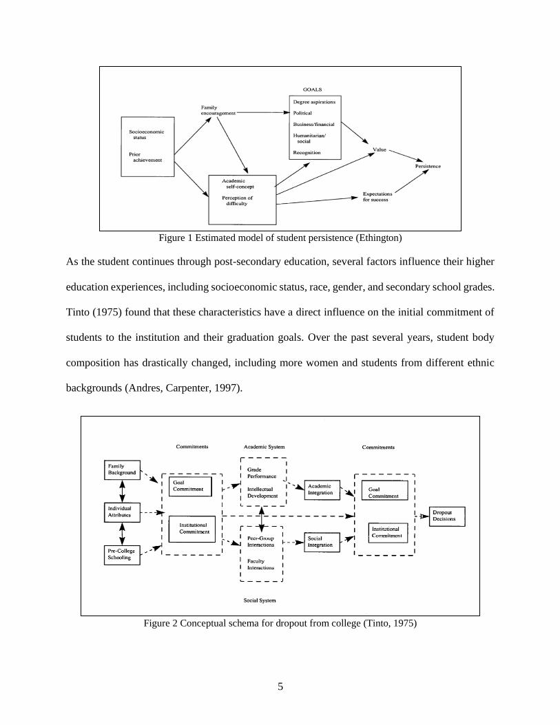
5

Figure 1 Estimated model of student persistence (Ethington)

As the student continues through post-secondary education, several factors influence their higher

education experiences, including socioeconomic status, race, gender, and secondary school grades.

Tinto (1975) found that these characteristics have a direct influence on the initial commitment of

students to the institution and their graduation goals. Over the past several years, student body

composition has drastically changed, including more women and students from different ethnic

backgrounds (Andres, Carpenter, 1997).

Figure 2 Conceptual schema for dropout from college (Tinto, 1975)

6

2.2.1 Distance (Proximity)

What Universities are nearby? This question plays a vital role in shaping educational opportunity

and equity for students. Studies of College enrollment and retention often overlook the question

about geography that affects their choices for educational destinations. Particularly for today’s

college, students who live in communities with few educational options are bound to accept

admission to a nearby institution (Hillman & Weichman, 2016). Another study based on the data

from High School and Beyond Survey showed that living near a specific 4-year college can expose

students to what these universities offer and encourage them to go to a particular 4-year school

(Do, 2004).

A study by Griffith & Rothstein (2009), which included 9000 youths (NLSY97) who were born

between the years 1980–1984, analyzed the factors which influenced the decision to apply to a

particular 4-year college. Results suggest that distance to a particular 4-year college significantly

affects the likelihood that a student applies to a specific school, which means that as the distance

to the nearest particular 4-year college increases, students are less likely to apply to this kind of

college irrespective of family income level.

A study designed to understand the characteristics and diversity of incoming students showed that

geography plays an important role; 57.4 percent of incoming students attending public four-year

colleges enroll within 50 miles from their permanent home (Eagan et al., 2015).

Pérez & McDonough (2008) focused on understanding the college choice process for Latina and

Latino students. The results demonstrated that first-generation college students, particularly

Latino, black, and Native American students depended heavily on family members and high school

contacts for purposes of college selection planning and are more likely to stay close to their home.

7

Using data from the Education Longitudinal Study of 2002 (ELS), a research study analyzed

15,362 students’ preferences for proximate colleges. The findings indicated that Asian and Latino

students and parents had stronger preferences for living at home during college compared to white

students and parents (Ovink and Kalogrides, 2015).

Studies of enrollment and graduation also include a factor of intrastate college student migration.

Alm & Winters (2009) conducted research using the data from 175 public school districts in

Georgia and examined the distance from a student’s home to the different Georgia state

institutions. The results indicate that student intrastate migration gets actively hindered by a greater

distance. However, black students are willing to migrate greater distances to attend HBCU

(Historically Black Colleges & Universities).

2.2.2 Race and Ethnicity

College enrollment rates and choice of majors over the last decade have varied by racial / ethnic

background.

From 2000 to 2016, college enrollment rates for White increased from 39 to 42 percent, the black

enrollment showed an increase from 31 to 36 percent, and Hispanic young adult enrollment rates

increased from 22 to 39 percent. Also, in terms of undergraduate enrollment the Hispanic college

population saw a 134 percent increase during this period whereas other racial/ethnic groups had

increased enrollment during the first part of this period, then began to decrease around 2010. In

2016, the female population had a higher percentage of undergraduates than males in all

racial/ethnic groups.

8

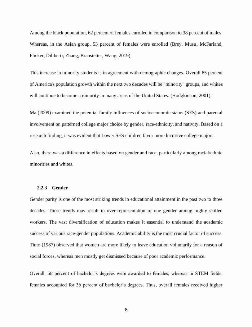
Among the black population, 62 percent of females enrolled in comparison to 38 percent of males.

Whereas, in the Asian group, 53 percent of females were enrolled (Brey, Musu, McFarland,

Flicker, Diliberti, Zhang, Branstetter, Wang, 2019)

This increase in minority students is in agreement with demographic changes. Overall 65 percent

of America's population growth within the next two decades will be "minority" groups, and whites

will continue to become a minority in many areas of the United States. (Hodgkinson, 2001).

Ma (2009) examined the potential family influences of socioeconomic status (SES) and parental

involvement on patterned college major choice by gender, race/ethnicity, and nativity. Based on a

research finding, it was evident that Lower SES children favor more lucrative college majors.

Also, there was a difference in effects based on gender and race, particularly among racial/ethnic

minorities and whites.

2.2.3 Gender

Gender parity is one of the most striking trends in educational attainment in the past two to three

decades. These trends may result in over-representation of one gender among highly skilled

workers. The vast diversification of education makes it essential to understand the academic

success of various race-gender populations. Academic ability is the most crucial factor of success.

Tinto (1987) observed that women are more likely to leave education voluntarily for a reason of

social forces, whereas men mostly get dismissed because of poor academic performance.

Overall, 58 percent of bachelor’s degrees were awarded to females, whereas in STEM fields,

females accounted for 36 percent of bachelor’s degrees. Thus, overall females received higher

9

percentages of bachelor’s degrees, but the lower percentage of bachelor’s degrees in STEM fields

was seen across all racial/ethnic groups (Brey et al., 2019).

Although some research studies assert that females are less persistent in engineering majors than

males (Adelman, 1998; Astin & Astin, 1992), more recent studies indicate that women admitted

to engineering majors are equally persistent as male students (Cosentino de Cohen & Deterding,

2009; Hartman & Hartman, 2006; Lord et al., 2009). Lord et al., 2009 examined the persistence of

engineering students based on gender and race/ethnicity utilizing a dataset of more than 79,000

students who enrolled in engineering at nine universities.

Results suggest that for Asian, Black, Hispanic, Native American, and White students, women

who enrolled in engineering are more likely to persist in engineering compared to another eighth-

semester destinations.

However, among Native Americans, rates are equivalent to those of men. Thus, the low

representation of women in the later years of engineering programs is a reflection of their low

representation at matriculation.

Ohland et al. (2011) examined race, gender, and measures of success in Engineering Education

using a Multiple-Institution Database for Investigating Engineering Longitudinal Development

(MIDFIELD). The results indicate that at all institutions, white women who enroll in engineering

tend to graduate in 4.6 years, whereas white men graduate in 4.8 years. Among Black students, the

average woman also completes the degree slightly faster than the average male student. Black

females exhibit average time-to-graduation of 4.8 years and 4.9 for Black males.

10

Figure 3 Number persisting to 8th semester (Ohland et al., 2011)

2.2.4 Internet

The internet has led to a seismic change in education. The impact of Digital Divide on college

access/ enrollment and educational equity is a major concern. It allows people to access quality

educational services from the comfort of their homes. From the college applications and access to

online content in the form of e-books to the implementation of virtual classrooms, technology-

based education opens new learning pathways.

Even in many industrialized countries, including the USA, Australia, UK, Netherlands, there is a

large percentage of students with no access to a computer with internet and e-mail at home. This

results in differences in digital skills between students (Volman, van Eck, Heemskerk, & Kuiper,

2005).

The entire college application process utilizes the internet, including school selection, sending

applications, and applying for financial aid. As per the data from NACAC (National Association

11

for College Admission Counseling), universities received 49 percent of their applications online

in 2005, 68 percent in 2007, which further increased to 94 percent by fall 2014 (Clinedinst et al.,

2015). The portal “Common App” lets students fill out a single application form for over 700

colleges across the country. Around 920,000 students used the Common App in the year 2015-16,

which were more than in 2008–09, when 31 percent of the applicants who used the portal were

first-generation students.

The statistics from NCES show that in 2015, 4 percent of students in the age group of 5 to 17 years

had home internet access without a subscription, and 11 percent of students had either only dial-

up access or no access to the Internet (National center of education statistics). Access to home

internet varies based on different racial/ethnic characteristics and geographic locale (File and Ryan

2014; Horrigan and Duggan 2015).

The digital divide had a significant impact on the ability to gain higher education access and social

capital (Pruijt, 2002; Fairlie, London, Rosner & Pastor, 2006; Bargh & McKenna, 2004; Venegas,

2007). The demographics that had less internet access included rural households, blacks, Latinos,

low SES, people with disabilities, people with no college education, and people over 50 years of

age.

Wilcox (2008) explored the correlation of the digital divide with college access and concluded that

the digital divide is about people’s access to universal information and knowledge. It is evident

that digital access contributes to college accessibility as students who face challenges in college

access lack digital access.

12

Over the past few years, there have been remarkable increases in students’ internet access

regardless of income, but still, a digital divide exists based on race, socioeconomic status, and

educational levels (Venegas, 2007). Children who used the internet more had higher scores on

standardized tests of reading achievement and higher-grade point averages (Jackson et al., 2006).

There is a noteworthy difference between the ways of internet usage and the differing attitudes

between male and female users towards the Internet (Bressers & Bergen, 2002; Cotten &

Jelenewicz, 2006; Odell et al., 2000; Jackson et al., 2001; Zhang, 2002; McMillan & Morrison,

2006).

Among U.S. college students, women's internet use is focused on educational and communicative

purposes, whereas men are more information-oriented and use the internet as a source of

entertainment. Also, both the gender showed similar uses of the internet academically (Fortson et

al., 2007). Irrespective of significant differences between Hispanic, Black non-Hispanic, and

White non-Hispanic students, all three racial groups were positive that the internet has a significant

impact on them in their academic lives (Jones, Yale, Millermaier, 2009).

Understanding the demographic characteristics of the student with no/limited access to internet

can help uncover equity gaps in education and also help inform policies to close these gaps (Moore,

Vitale, Stawinoga, 2018).

As per U.S. Census Bureau (2013-2017 American Community Survey 5-Year Estimates), 86.5

percent of households in Michigan have one or more types of computing devices, out of which 77

percent of households have an Internet subscription comprising of 76.3 percent with a broadband

connection and remaining 0.7 percent with Dial-up connections. Based on race/ethnicity,

broadband Internet subscription percentage are lowest for African Americans (66.7 percent), and

13

highest for Asians (91.4 percent), whereas 76.8 percent of Hispanics or Latinos (of any race) and

83.3 percent of Whites have broadband Internet subscription.

2.2.5 Income- (Household Income and Neighborhoods Poverty Level)

Past research examining the connection between household income, neighborhood poverty level,

and educational attainment have found essential relationships.

According to Harold Hodgkinson, a renowned demographer, "If you know household income and

the education level of the parents in America, you can predict about 45 percent of the variation on

the national assessment scores without knowing anything about race." (Goldberg, Kappan,

Bloomington, 2000).

Belley and Lochner (Belley, Lochner, 2007) found a considerable increase in the effect of family

income on college attendance over time. Kinsler, Pavan (2011) observed that family income had

a significant effect on the quality of higher education, especially for high-ability individuals.

However, this effect has declined substantially over time for high ability students.

Harding (2003) found a causal effect of neighborhoods on the high school drop-out rate. He

observed two groups of children of the same ages (10 years old) in different neighborhoods. The

students in high-poverty neighborhoods were more likely to drop out of high school as compared

to those in low-poverty neighborhoods.

Students mainly characterized by low socioeconomic status (SES) must overcome multiple hurdles

and build self-regulation, control, and competence to achieve educational and occupational success

14

and avoid delinquent behaviors and school failure. (Brody, Kogan, & Grange, 2012; Wills et al.,

2011; Chen et al., 2014).

The neighborhood is a crucial parameter; teenagers spend a majority of time outside their home

and with their peers. In high-poverty neighborhoods, this social parameter can result in potentially

dangerous risk factors such as violent crimes and peer pressure related to substance use (Collins

& Laursen, 2004; Chen & Miller, 2013).

2.2.6 Scholarships/ Pell Eligibility

2.2.6.a Effects on Enrollment

In recent years, the government has tried to improve gaps in college access and accomplishment

by giving need-based grants. Educational cost is on the rise nation-wide, and scholarships offer

access to higher education. Regardless of enormous increases in higher education enrollment in

recent years, the college attendance rates of youth from low-income families continue to decrease

(Doyle & Skinner, 2017). Scholarships based on financial need can be vital tools for increasing

college access for low-income students.

Heller & Marin (2002) conducted a study investigating scholarships’ influence on attendance.

Georgia’s HOPE (Helping Outstanding Pupils Educationally) Scholarship suggested that for each

$1,000 of subsidy offered by HOPE, the college attendance rate increased by around four

percentage points and it had a considerably more significant impact on whites than on blacks. Also,

theory and empirical evidence were incapable of predicting that aid has its most potent effect on

disadvantaged youth.

15

Ness, Tucker (2008) analyzed Under-represented Student Perceptions about Tennessee’s Merit

Aid Program. The results demonstrated that African American and low-income students were

bound to see their eligibility for merit-based grants as affecting their choice on whether to go to

college.

A study from Heller (2006) has shown that merit aid is more likely to be granted to students from

higher-income families as compared with need-based grants, which in contrast, are significantly

more likely to benefit lower-income students. Similarly, studies have shown that white students

receive a disproportionate share of the merit aid money. Such outcomes affect students from

traditionally underrepresented populations who receive proportionally less financial aid, which

significantly impacts their ability to enroll and persist in college.

A study from Pluhta & Penny (2013) presented findings of a public community college with an

approximate enrollment of 7,600 students in 2007 which offered a Promise Scholarship to all

graduating students at the participating high school to attend the local community college tuition-

free for one year regardless of financial need or academic achievement. And the outcomes

demonstrated a positive effect on college application rates, especially for the low-income minority

students from an inner-city high school.

2.2.6.b Effects on Retention

A report from Ratledge et al. (2019) discussed the outcomes of Detroit’s Promise program, which

intends to encourage college attendance of underserved students in Detroit, Michigan. A Detroit

Promise Path was made with the cooperation of MDRC (Manpower Demonstration Research

Corporation) and the Detroit Promise to assist students after getting enrolled in college where,

16

students were given monthly gift card refilled with $50 each month to attend coaching meetings.

The results suggested a positive impact on students’ persistence in school, full-time enrollment,

and credit accumulation, along with positive relationships with their coaches.

Bartik et al. (2017) conducted a study to estimate the effects of the Kalamazoo Promise on

postsecondary education. Results indicated an increase in college enrollment, college credits

attempted, and credential attainment—also, substantial effects on women and minorities.

Castleman, long (2016) analyzed the impacts of the FSAG (Florida Student Access Grant) utilizing

a regression-discontinuity design and exploiting the cut-off used to decide eligibility. The results

showed that grant eligibility positively affected attendance, especially at public 4-year institutions.

In a report, Nichols (2015) analyzed the graduation rate for Pell Grant recipients at 1,149 four-year

public and private nonprofit institutions. It showed that there is a 14-point graduation gap between

Pell and non-Pell students at the national level, whereas, the average graduation gap at the

institutional level is only 5.7 percentage points.

17

Chapter 3. Purpose of Study

Despite the very substantial literature on college enrollment trends in higher education, much

remains unknown about the nature of a student’s enrollment decision. From a broad perspective,

previous research works depict the relationship between a student’s background characteristics

and enrollment trends. We know that students who enroll in universities come from a variety of

socio-economic and demographic backgrounds, which includes attributes such as differences in

sex, race/ethnicity, pre-college experiences. Each of these attributes has a direct or indirect effect

on the student’s decision to enroll in an institution of higher education. More importantly, from

the institutional perspective, inadequate attention given to identifying target populations requiring

specific forms of assistance is a significant concern.

This study is an attempt to use and elaborate on Tinto’s (1975) perspective (guiding theory) to

address and investigate the demographic differences of students entering an engineering program

at the University of Michigan-Dearborn and examine the relationship between selected student

background characteristics and the student enrollment. This research does not state that these

factors exclusively are responsible for the lower enrollment of students in the engineering domain

from particular geographic areas. But these demographic characteristics may be of importance to

the decision-makers when designing specific strategies to attract and retain more students focusing

on particular geographic areas.

18

The results of this thesis may prove beneficial in the identification of specific Zip Codes with lower

student enrollment and higher likelihood of attrition and suggest methodical interventions to

improve the enrollment and persistence of students from vulnerable areas.

19

Chapter 4. Proposed Research Question

This study seeks to extend the current literature on student enrollment, transfer, and retention by

addressing the following research questions:

1) In what ways does student background characteristics predict enrollment and retention

trends?

2) Which of the socio-economic characteristics influence the likelihood of students enrolling

and majoring in CECS at the University of Michigan- Dearborn?

3) Which Zip Codes in Michigan should be considered for strategies seeking to attract,

engage, and retain students?

20

Chapter 5. Methodology

This study involves 9034 students (2015 - 2019 enrollment count) enrolled in the College of

Engineering and Computer Science department at the University of Michigan-Dearborn. The

enrollment data used here were obtained from the College records (University of Michigan-

Dearborn), and the demographic characteristics of 269 Michigan Zip Codes where the students

were from was obtained from the US Census database. All attributes and analyses used in this

study were specifically designed for students living in Michigan, and student identities were kept

anonymous to protect students’ identity. Human subject research approval has been given to

conduct this research.

The variables by Zip Code used in this study included: (1) Enrollment Count of students in CECS

Department at UM-Dearborn, (2) Median Household Income ($), (3) Number of Households, (4)

Number of Households with internet access, (5) Travel Distance to UM-Dearborn, (6) Number of

People with bachelor’s degree and above, (7) Number of People who are high school graduate and

above, (8) Total Population, (9) Number of College Eligible people (18 – 24 years old), (10)

Population below 200 percent of the poverty level, (11) Minority Population.

21

Table 1 Data distribution

Sr.

No.

Variable by

Zip Code

Minimum First

Quartile

Median Mean Third

Quartile

Maximum

1 Student

Enrollment

Count

1 3 9 33.58 24 775

2 Median

Household

Income ($)

20505 45422 58913 62195 76685 140372

3 Number of

Households

92 4450 8282 8605 11574 25435

4 Number of

Households

with internet

access

83 3537 6247 6785 9235 21264

5 Travel

distance to

UM-

Dearborn (mi)

0 18.10 33 52.96 60.40 278.70

6 Number of

people with

bachelor’s

degree or

above

90 2531 5227 6986 9897 40237

7 Number of

People who

are high

school

graduate and

above

166 10649 18770 19829 26384 62421

8 Total

Population

166 11886 21128 22037 29824 67775

9 Eligible

population

15 876 1712 2193 2802 21731

10 Number of

People below

poverty level

20 2283 4748 6920 8953 36594

11 Minority

Population

0 714 2846 5854 7051 45783

22

5.1 Feature Selection

Managing a vast number of input features/ high-dimensional data is sometimes a challenging task

for researchers. In recent years, data has gotten progressively bigger in both the number of

instances and number of features in numerous applications, for example, genome projects (Xing

et al., 2001), client relationship management (Ng & Liu, 2000). This enormity may significantly

degrade the performance of learning algorithms. It requires pre-processing of data where feature

selection is one of the most common and significant techniques. In statistics, feature selection, also

known as variable/ attribute selection, is mainly used for distinguishing important features and

removing unessential and redundant information. Usually, unessential and redundant information

is those variables that give no more helpful information than the currently selected features.

It makes feature selection extremely vital when facing high dimensional data these days.

Researchers and practitioners understand that to utilize data mining tools viably, data pre-

processing is fundamental to efficient data mining.

Feature selection algorithms designed with various assessment criteria essentially fall into three

classes: the filter model, the wrapper model, and the hybrid model (Liu, Yu, 2005). The filter

model depends on the general attributes of the data to assess and select feature subsets without

including any mining algorithm. The wrapper model requires one predetermined mining algorithm

in feature selection and uses its performance as they assess and decide which features are selected.

It needs to learn a hypothesis for each new subset of features and searches for features better suited

to the mining algorithm to improve learning performance; however, it will be more

computationally costly than the filter model (Yu, Liu, 2003). The hybrid model endeavors to

exploit the two models by using several evaluation criteria in various search stages (Liu, Yu, 2005).

23

Canedo, Maroño, Betanzos (2012) utilized several synthetic datasets for reviewing the

performance of feature selection methods in the presence of irrelevant features and redundancy

between attributes and also with a small ratio between several samples and number of features. It

was an effective way to understand and choose a robust method.

In general, the feature selection has four key steps that include Subset Generation, Evaluation of

Subset, Stopping Criteria, Result Validation (Kumar, 2014).

Feature Selection helps us to determine the smallest set of features that are needed to predict the

response/target variable with high accuracy. In this study, initially there are 10 features (1) Median

household income, (2) Number of households, (3) Number of households with internet access, (4)

Travel distance to University, (5) Number of people with bachelor’s degree or above, (6) Number

of People who are high school graduate and above, (7) Total Population (8) Eligible population

(9) Number of People below poverty level (10) Minority Population. We want to predict the

correlation/ dependency of the Students Enrollment Count (target/ response variable).

In this research, feature selection included (1) Significant features from Negative Binomial

Regression and (2) Lasso Regression. Thus, reliability of factors was established by selecting

significant features from Negative Binomial Regression and Lasso Regression.

5.1.1 GLM- Negative Binomial Regression

The General Linear Model (GLM) is a useful system for comparing how a few variables influence

different continuous variables.

GLM is depicted as: Data = Model + Error (Rutherford, 2001, p.3)

24

Negative binomial regression is a type of generalized linear model wherein the dependent variable

is a count of the occurrence of an event. Negative binomial regression is commonly recommended

to handle overdispersion. In general, overdispersion occurs when the variance exceeds the mean.

The regression analysis model is based on numerous assumptions, which include absence of

multicollinearity, non-homogeneity, linearity, and autocorrelation (Osborne, Waters, 2002). At a

point, if any of these assumptions are violated, then the model is not reliable or acceptable in

estimating the population parameters. Negative binomial regression has numerous assumptions,

for example, linearity in model parameters, independence of individual observations, and the

multiplicative effects of independent variables. Also, negative binomial regression permits the

conditional variance of the result variable to be higher than its conditional mean, which offers

greater flexibility in model fitting (Yang, Berdine, 2015).

Several researchers have used negative binomial regression for the analysis of over-dispersed

count data. Alexander et al. (2000) presented a spatial model for the mean and correlation of highly

dispersed count data, using a negative binomial distribution. Boveng et al. (2003) used a

generalized additive model (negative binomial regression), which provided an adjustment for the

covariates, and also confirmed the nature and shape of the covariate effects.

5.1.1.a Multicollinearity

The multicollinearity is an exact linear relation among two or more input variables (Hocking,

1983). The presence of various (linearly) correlated features makes the model unstable, which

implies that minor changes in the data can cause enormous changes in the coefficient values of the

model, making model interpretation exceptionally difficult. Likewise, analytical limitations

25

identified with collinearity require us to redefine the approach to select variables, rather than

adopting a naive approach where we indiscriminately utilize all data for analysis.

Multicollinearity is a phenomenon when two or more predictors in a multiple regression model are

highly correlated. It leads to an increase in the standard error of the coefficients (Daoud, 2017).

Furthermore, increased standard errors make a few factors statistically insignificant when they

ought to be significant. On the other hand, if there is no linear relationship between predictor

variables, they are termed as orthogonal (Jensen, Ramirez, 2013).

At the point when two or more features are highly correlated, the relationship between the

independent and the dependent variables is contorted by the strong connection between the

independent variables, which in turn leads to the likelihood of incorrect interpretation and results.

Thus, if the variables are perfectly correlated, the regression is unlikely to be computed (Milliken,

Johnson 2002).

5.1.1.b Variance Inflation Factor (VIF)

A straightforward way to identify and deal with collinearity among explanatory variables is the

use of variance inflation factors (VIF). VIF estimations are clear and easily understandable; higher

VIF value depicts the higher collinearity.

A VIF for a single feature is acquired utilizing the r-squared estimation of the regression of that

feature against all other features (explanatory variables). A VIF is determined for each feature, and

those features with ‘high’ VIF values (5-10) are removed.

26

Lin, Foster, and Ungar (2011) have shown that classical VIF regression outperforms many other

models, including stepwise regression, Lasso, FoBa, and GPS.

VIFj = 1

1 − Rj2

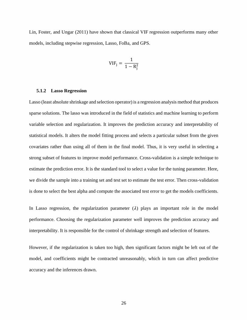
5.1.2 Lasso Regression

Lasso (least absolute shrinkage and selection operator) is a regression analysis method that produces

sparse solutions. The lasso was introduced in the field of statistics and machine learning to perform

variable selection and regularization. It improves the prediction accuracy and interpretability of

statistical models. It alters the model fitting process and selects a particular subset from the given

covariates rather than using all of them in the final model. Thus, it is very useful in selecting a

strong subset of features to improve model performance. Cross-validation is a simple technique to

estimate the prediction error. It is the standard tool to select a value for the tuning parameter. Here,

we divide the sample into a training set and test set to estimate the test error. Then cross-validation

is done to select the best alpha and compute the associated test error to get the models coefficients.

In Lasso regression, the regularization parameter (𝜆) plays an important role in the model

performance. Choosing the regularization parameter well improves the prediction accuracy and

interpretability. It is responsible for the control of shrinkage strength and selection of features.

However, if the regularization is taken too high, then significant factors might be left out of the

model, and coefficients might be contracted unreasonably, which in turn can affect predictive

accuracy and the inferences drawn.

27

Lasso limits the residual sum of squares and generates some coefficients, which are precisely zero

and thus give interpretable models (Tibshirani, 1995). Lasso regression consists of L1

regularization, which adds a penalty equivalent to the absolute estimation of the magnitude of the

coefficients. It results in sparse models with few coefficients; the regularization parameter controls

the strength of the L1 penalty, i.e., it makes non influencing coefficients to zero and eliminates

them from the model.

5.2 Data Visualization Using QGIS

A geographic Information System (GIS) helps to capture, store, analyze, manage, and visualize

data and associated information that is spatially referenced to Earth (Eray, 2012). It is an

application of information technology that allows people to solve many geographic problems

quickly, effectively, and easily with the ability to make analysis, especially location analysis, in

combination with traditional database systems.

According to De Grauwe, GIS helps in data visualization by projecting tabular data onto maps and

providing more flexible assistance in prospective planning at various levels of analysis including

national, regional, provincial, and local (De Grauwe, 2002).

Geographic information systems (GIS) technology and methods have made geographic analysis

accessible to the desktop computer. Thus, it has transformed decision-making in society (Kerski,

2003). A GIS can be used to visualize the spatial relationships among real-world features. Many

different types of information can be analyzed and contrasted using GIS, including information

about income or education level. GIS also allows for modeling the results of an action or policy

implementation. Nowadays, GIS can assist educational planning related to the allocation of

28

resources, proficiency of schools, and improving learning effectiveness. Geographic Information

System (GIS) assists individuals in taking care of numerous geographic issues rapidly, viably, and

effectively with the capacities to make location analysis.

In this research, GIS helps us to present a clear picture of educational facilities and solve the

persisting problem of low enrollment trends in educational industries by focusing on geographic

characteristics of areas from where students live. It helps us in determining the scope of

improvement in college policies to increase college enrollment. The applicability of GIS in

Education will assist decision-makers to support educational decisions by senior administration,

which affects students’ chances of enrolling in a University. Thus, QGIS was used for data

visualization in the preliminary stage to analyze the enrollment trends at the University of

Michigan-Dearborn.

5.3 Spearmen Correlation Analysis

Now the next step was to find the linear relationship between demographic factors and their effect

on college enrollments. It was done using the Spearmen Correlation analysis, which gave us the

factors which were moderately and strongly correlated to enrollment trends.

The Spearman Correlation Coefficient is a rank-based, nonparametric method to assess the linear

relationship between two random but continuous variables using a monotonic function. The

statistical significance of Spearman correlation coefficient ranges from +1 to -1, where “+1” points

towards a strong positive correlation, whereas a “-1” indicates a perfect negative correlation of

random variables.

29

Spearman rank correlation helps to analyze whether the two ranked variables covary, i.e., with the

increase in one variable the other variable tends to increase or decrease. With one measurement

variable and one ranked variable, the measurement variable needs to be converted to ranks and

Spearman rank correlation used on the two sets of ranks (McDonald, 2015).

5.4 Cluster Analysis

At a low and practical level, we wish to separate the varieties into distinct groups as often as we

can without too frequently separating varieties that should stay together (Tukey, 1949). Whereas,

in research, Plackett suggested the possibility of using cluster analysis in place of a multiple

comparison technique for grouping the treatment means (O’Neill, Wetherill, 1971).

To accomplish a variety of research objectives, there is sometimes a need to find out which objects

in a set are similar and dissimilar. Mathematical methods such as cluster analysis achieve this task

mathematically. This quantitative method gathers the items with similar descriptions

mathematically into the same cluster by sorting objects described as data. (Romesburg, 2004).

Cluster Analysis has been used for a variety of purposes ranging from segmentation of consumers

in cluster analysis to the identifying of groups of schools or students with similar characteristics.

In the early days, such clustering was based only on the perception and judgment of the researcher.

However, more recently objectivity standards of modern science have given rise to automatic

classification procedures (Rousseeuw, 2009).

30

Hybels et al. (2009) used latent class cluster analysis to explore the profiles of depressive

symptoms in older adults who are diagnosed with major depression and identified homogeneous

clusters of individuals based on symptom profiles.

Jennings (2008) used Cluster Analysis to define rating territories for personal lines insurance in

the United States. It created homogeneous groupings of geographic areas with similar exposure to

the risk of insurance losses.

In a study based on Bahr’s behavioral typology, variation in patterns of students’ use of 105

community colleges in California was observed, and colleges were classified into five types using

k-means cluster analysis. This classification was based on dominant or disproportionate patterns

of use (Bahr, 2013).

In another study, survey data comprising of 663 community colleges from the Center for

Community College Student Engagement was used to examine the existing similarities and

differences in student engagement in community colleges based on k-means cluster analysis

(Saenz, Hatch, Bukoski, Kim, Lee, Valdez, 2011).

The research described the students involved in the search phase of the college choice process,

where students were identified into five unique clusters that differed from each other based on

various academic, demographic, and personal characteristics. Further analysis of these clusters

comprised of students with similar backgrounds and goals for higher education (Shaw, Kobrin,

Packman, Schmidt, 2009).

Recent work on concurrent enrollment examined how educators and students categorize students’

motivations to select concurrent enrollment through a group concept mapping process. Multi-

31

dimensional scaling and hierarchical cluster analysis were applied to the grouped data to create a

cluster map of the educators’ categorizations. Furthermore, some differences were observed

between educators’ and students’ maps (Dare, Dare, Nowicki, 2017).

To design adequate strategies to attract, engage, and retain students in UNITEC’s Faculty of

Engineering and Architecture, the categorization of the municipalities was done by using

multivariate analysis and cluster. Similar characteristics were grouped to create a typology to

understand the distinctive characteristics of the hometowns of the students (Arzu, Valle, 2018).

In this research, there was a need to identify the groups of Zip Codes, which can be classified into

clusters sharing similar demographic characteristics. This objective was achieved with the help of

cluster analysis.

5.5 Control Group Analysis

To specifically deal with the areas which lack some significant attributes. It was of foremost

importance to compare the characteristics of Zip Codes of high enrollment count to those Zip

Codes with low enrollment counts. This was done using control group analysis, which compared

the differences in demographic characteristics of Zip Codes.

32

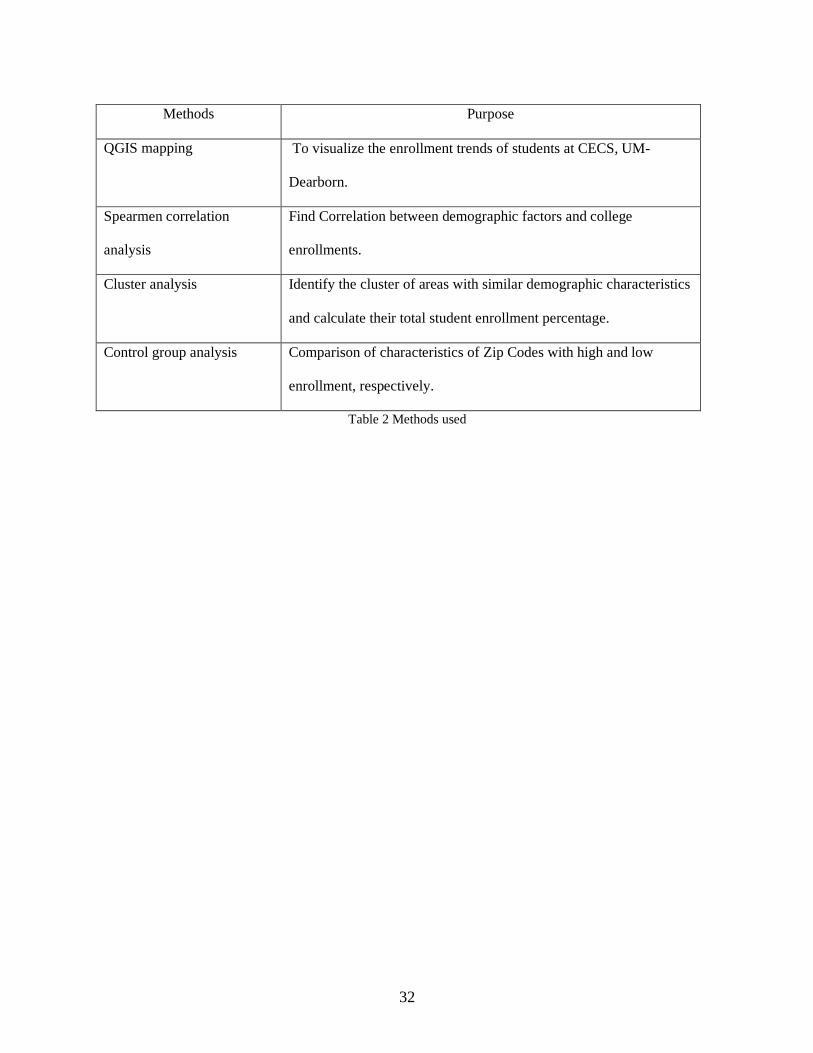
Table 2 Methods used

Methods Purpose

QGIS mapping To visualize the enrollment trends of students at CECS, UM-

Dearborn.

Spearmen correlation

analysis

Find Correlation between demographic factors and college

enrollments.

Cluster analysis Identify the cluster of areas with similar demographic characteristics

and calculate their total student enrollment percentage.

Control group analysis Comparison of characteristics of Zip Codes with high and low

enrollment, respectively.

33

Chapter 6. Results

6.1 Feature Selection

Here, Feature selection included (1) Significant features from Negative Binomial Regression and

(2) Lasso Regression.

6.1.1 GLM- Negative Binomial Regression:

Here, the Negative Binomial Regression model was used for selecting and interpreting variables,

which is based on using coefficients of the regression model to select the essential features.

Initially we started with ten variables, but the output of Regression model gives us eight variables

which depicts the presence of multicollinearity (Table 3).

In a statistical model, collinearity among explanatory variables can complicate or forestall the

identification of an optimal set of features. We need to identify every significant feature to describe

associations with the target variable more precisely

34

Table 3 Negative binomial regression model

VIF gives the combined effect of dependencies among the regressors on the variance of that term.

Here the maximum VIF is 148.104205, which shows that a multicollinearity problem exists in this

dataset. Furthermore, utilizing the VIF can help identify which regressors are responsible for the

multicollinearity. The square root of the variance inflation factor depicts the variation in standard

error in comparison to zero correlation of that specific factors to other predictor variables in the

model (Table 4).

Coefficients:

Variables by Zip Code Estimate Std. Error T value Pr(>|t|)

(Intercept) 2.796e+00 4.349e-01 6.428 6.14e-10 ***

Median household income

($)

8.020e-07 5.362e-06 0.150 0.88123

Number of Households -1.621e-04 1.940e-04 -0.836 0.40391

Number of Households

with Internet Access

2.771e-04 2.227e-04 1.244 0.21457

Travel Distance to UM-

Dearborn

-2.478e-02 2.335e-03 -10.612 < 2e-16 ***

Population with bachelor’s

degree and Above

5.969e-05 3.347e-05 1.783 0.07572

Number of college eligible

people

-1.807e-04 6.617e-05 -2.730 0.00676 **

Number of people below

poverty level

1.326e-04 4.037e-05 3.284 0.00116 **

Minority population -6.419e-05 1.955e-05 -3.283 0.00117 **

Aic: 20453

35

Table 4 Initial variance inflation factor (VIF)

In the next step, the regressors responsible for the multicollinearity were removed. The updated

regression model is much improved compared with the original. We see a decrease in the number

of features that are significantly related to the target variable. This decrease is directly related to

the standard error estimates for the parameters (Table 5).

Factors VIF

Median Household Income

2.805109

Number of Households 148.104205

Number of Households with internet access

131.740509

Travel Distance to UM-Dearborn

1.496327

Number of People with bachelor’s degree and above

7.521675

Number of College Eligible people (18 – 24 years old).

4.076598

Number of people below poverty level

11.525756

Minority Population

4.375310

36

Table 5 Final variance inflation factor (VIF)

In the regression model, three asterisks represent a highly significant p-value. A p-value of 0.05 or

less is a good cut-off point Thus, a small p-value for the intercept and the slope shows that we can

reject the null hypothesis, which permits us to presume that there is a strong relationship between

features and response variables. AIC (Akaike information criterion) is used as an estimator of

relative goodness of fit of the model for a specific set of data (Table 6).

Factors VIF

Median Household Income 2.426643

Travel Distance to UM-Dearborn 1.511012

Number of People with bachelor’s degree and above 4.472690

Number of People who are high school graduate and above 3.337724

Number of College Eligible people (18 – 24 years old) 2.914366

Minority Population 1.883107

37

Coefficients:

Variable by Zip Code Estimate Std. Error t value Pr(>|t|)

(Intercept) 3.134e+00 3.933e-01 7.967 4.99e-14 ***

Median Household Income -4.342e-06 5.085e-06 -0.854 0.394

Travel Distance to UM-Dearborn -2.534e-02 2.393e-03 -10.593 < 2e-16 ***

Number of People with bachelor’s

degree and above

9.660e-06 2.613e-05 0.370 0.712

Number of People who are high school

graduate and above

7.099e-05 1.266e-05 5.608 5.18e-08 ***

Number of College Eligible people (18

– 24 years old)

-4.162e-05 5.614e-05 -0.741 0.459

Minority Population -5.136e-05 1.291e-05 -3.979 8.98e-05 ***

AIC: 20682

Table 6 Final regression model

In our model, the factors Median Household Income, Travel Distance to UM-Dearborn, Number of

People who are high school graduate and above have low p-value which shows that they are

significant predictors in our analysis.

6.1.2 Lasso Regression

Lasso Regression performs the variable selection by imposing a constraint on the features which

affects the regression coefficients for some features and shrink them to zero. The plot shows the

optimization of Lasso in terms of choosing the best Regularization Parameter (𝜆) (Figure 4).

Furthermore, features with a regression coefficient equal to zero are eliminated from the model

whereas, features with non-zero regression coefficients are strongly related with the response

(Table 7).

38

Figure 4 Regularization parameter (𝜆)

Coefficients:

Intercept 2.859765e+00

Median Household Income 0.000000e+00

Travel Distance to UM-Dearborn

-2.184679e-02

Number of People with bachelor’s degree and above

0.000000e+00

Number of People who are high school graduate and above

6.000622e-05

Number of College Eligible people (18 – 24 years old)

0.000000e+00

Minority Population

-3.463263e-05

Table 7 Lasso regression coefficients

39

Statistically chosen factors include Travel Distance to UM-Dearborn, Number of People who are

high school graduate and above, Minority Population.

Factors selected based on the literature include: Median Household Income, Number of College

Eligible people (18 – 24 years old), Number of households with internet access, Total Population.

Final features selected in this study include:

Sr. No. Features (Variable by Zip Code)

1 Travel Distance to UM Dearborn

2 Number of People who are high school graduate and above

3 Minority Population

4 Median Household Income

5 Number of College Eligible people (18 – 24 years old)

6 Number of households with internet access.

7 Total Population

Table 8 Final selected features

6.2 Data Visualization Using QGIS

In the preliminary analysis, student enrollment data (number of students enrolled at UM-Dearborn

along with their Zip Code in Michigan) and open-source data from the US Census is utilized to

investigate the role of demographic profiles of the students’ home Zip Codes on college access.

The data is visualized graphically using QGIS to observe the differences in demographic

characteristics by Zip Codes.

40

The maps indicate a clear difference in the student demographics as represented by Zip Codes. It

gave a clear indication of which factors should be investigated further. Southeast Michigan has

the highest representation of students admitted to the UM-Dearborn CECS during the years 2015

to 2019 (Figure 5).

More than half of the state’s population is located in Southeast Michigan together with a majority

of the state’s industries and businesses. So, the large cluster of enrollment counts from this area is

expected for a metropolitan college.

Figure 5 UM-Dearborn CECS undergraduate enrollment count of year (2015 - 2019) from respective Zip Codes

41

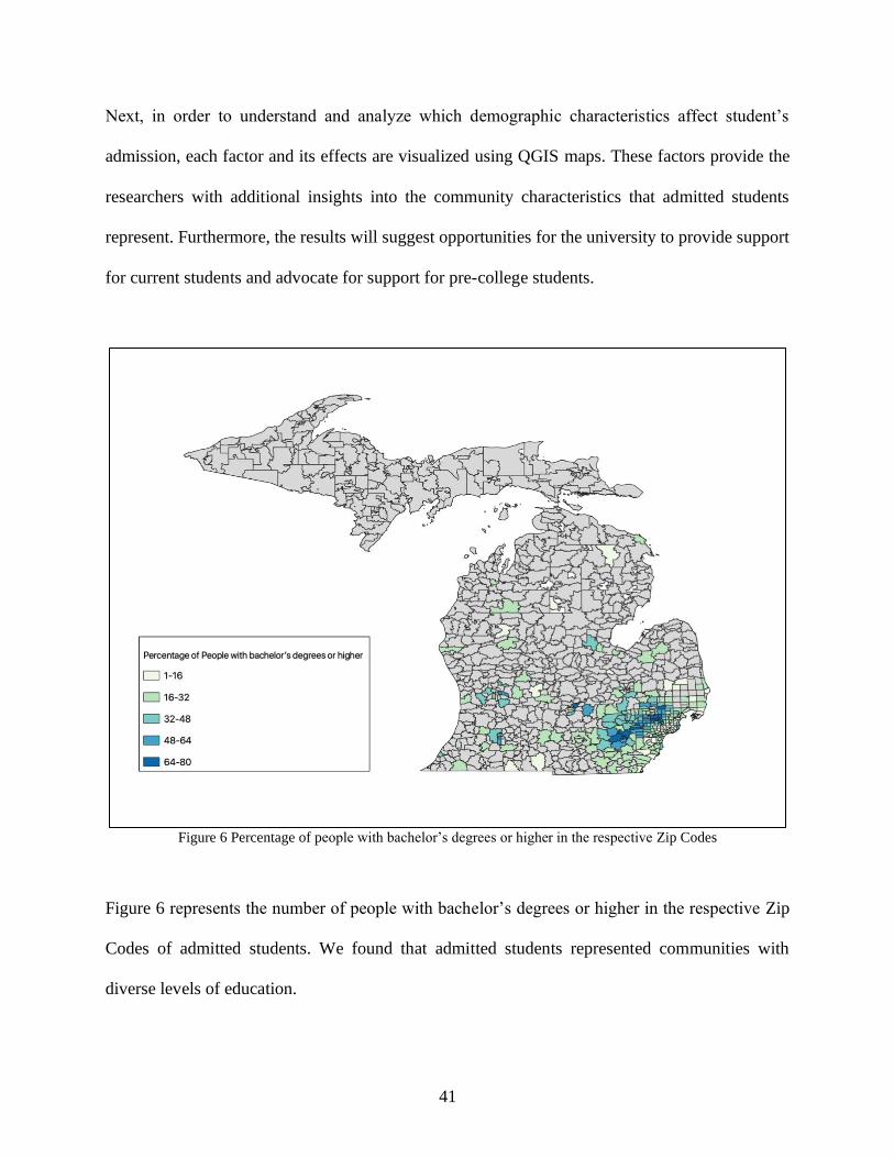
Next, in order to understand and analyze which demographic characteristics affect student’s

admission, each factor and its effects are visualized using QGIS maps. These factors provide the

researchers with additional insights into the community characteristics that admitted students

represent. Furthermore, the results will suggest opportunities for the university to provide support

for current students and advocate for support for pre-college students.

Figure 6 Percentage of people with bachelor’s degrees or higher in the respective Zip Codes

Figure 6 represents the number of people with bachelor’s degrees or higher in the respective Zip

Codes of admitted students. We found that admitted students represented communities with

diverse levels of education.

42

Also, the highest number of admitted students represented Zip Codes with the highest density of

college-educated people. This diverse education distribution can also be seen from Figure 7 which

tells us about the population with high school graduation and above.

Figure 7 Percentage of people with high school graduation or higher in the respective Zip Codes in Michigan

The distribution pattern of Median household Income in respective Zip Codes, ranges from

$20,505 to $140,372, which denotes a significant diversity in terms of affordability (i.e., access to

basic needs). The overall U.S. median income was $55,775 (2015) and $63,030 (2019), which

shows a significant difference in income diversity. This variation in median household income

across Zip Codes gives information about the social class and the lifestyle of students on campus

(Figure 8).

43

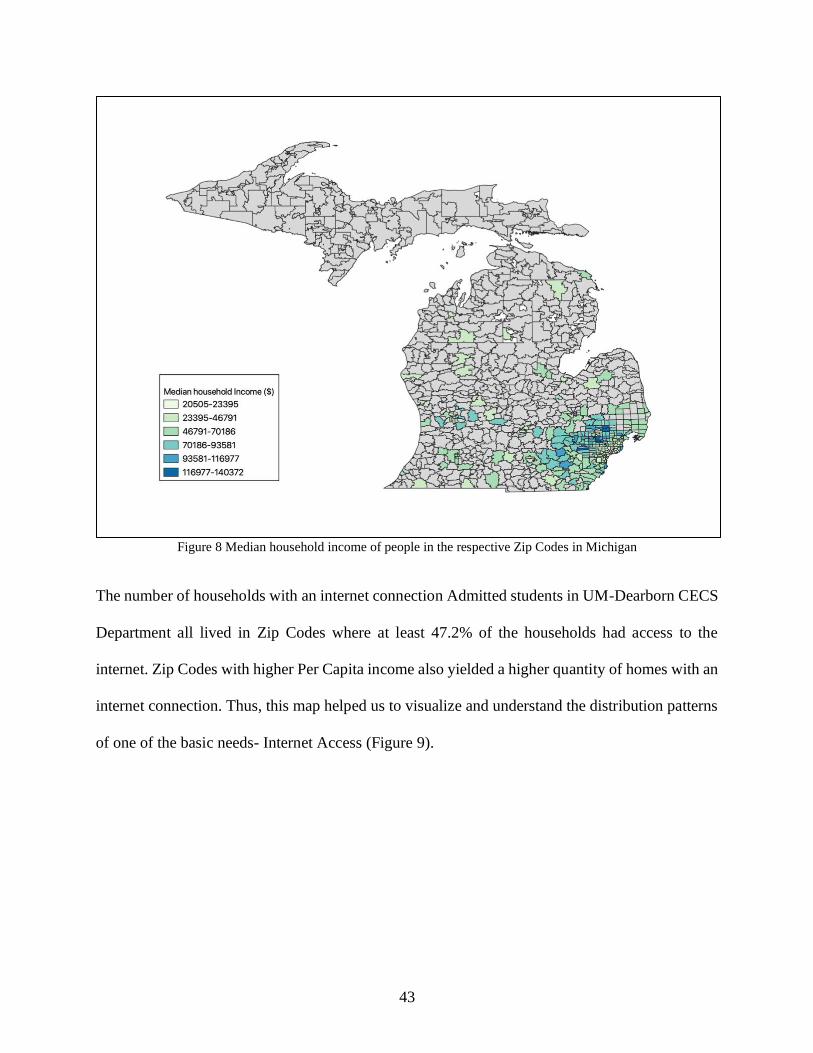
Figure 8 Median household income of people in the respective Zip Codes in Michigan

The number of households with an internet connection Admitted students in UM-Dearborn CECS

Department all lived in Zip Codes where at least 47.2% of the households had access to the

internet. Zip Codes with higher Per Capita income also yielded a higher quantity of homes with an

internet connection. Thus, this map helped us to visualize and understand the distribution patterns

of one of the basic needs- Internet Access (Figure 9).

44

Figure 9 Percentage of households with internet access in the respective Zip Codes in Michigan

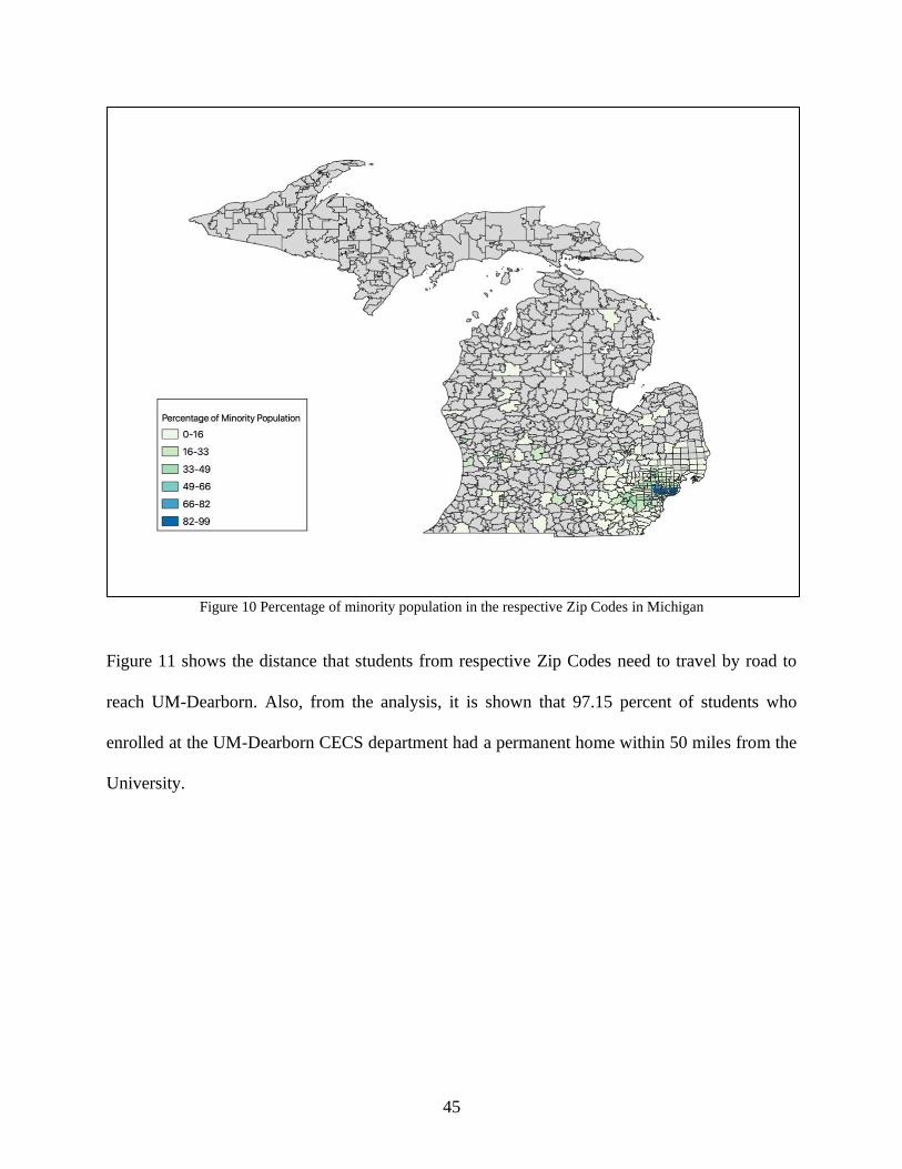
The impact of racial diversity in Zip Codes from which students are admitted may play an essential

role in their enrollment decision. Eighty seven percent of the Zip Codes students are from have a

minority population of less than 50 percent (Figure 10).

45

Figure 10 Percentage of minority population in the respective Zip Codes in Michigan

Figure 11 shows the distance that students from respective Zip Codes need to travel by road to

reach UM-Dearborn. Also, from the analysis, it is shown that 97.15 percent of students who

enrolled at the UM-Dearborn CECS department had a permanent home within 50 miles from the

University.

46

Figure 11 Travel distance to UM- Dearborn from the respective Zip Codes

47

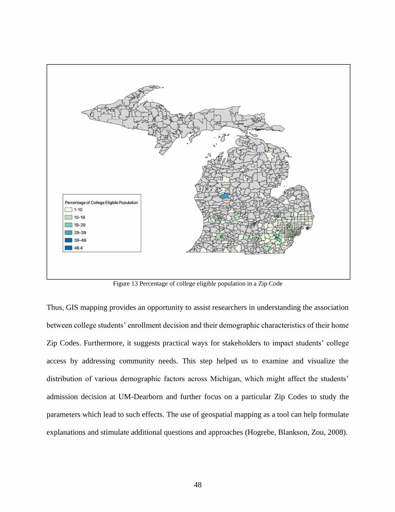
Figure 12 Total population in a Zip Code

Figure 12 shows the population distribution of the Zip Codes from which students enrolled at UM-

Dearborn originate. This visualization has helped us to analyze the population differences across

Zip Codes. Similarly, Figure 13 shows us the college eligible population within each Zip Code

where, college eligible age group is defined as age group between 18 to 24 years.

48

Figure 13 Percentage of college eligible population in a Zip Code

Thus, GIS mapping provides an opportunity to assist researchers in understanding the association

between college students’ enrollment decision and their demographic characteristics of their home

Zip Codes. Furthermore, it suggests practical ways for stakeholders to impact students’ college

access by addressing community needs. This step helped us to examine and visualize the

distribution of various demographic factors across Michigan, which might affect the students’

admission decision at UM-Dearborn and further focus on a particular Zip Codes to study the

parameters which lead to such effects. The use of geospatial mapping as a tool can help formulate

explanations and stimulate additional questions and approaches (Hogrebe, Blankson, Zou, 2008).

49

Mapping of the demographic variables with enrollment trends for visual analysis leads us to a

better understanding of relationships that have influenced enrollment. For example, if a student is

living in a home which is at or below the poverty level, they might lack access to basic needs (i.e.,

electricity at home, resources for school supplies, computer, and technology, transportation) to

prevail in the studies.

The preliminary research provides encouragement to further the investigation and analyze different

factors that may affect the success of underrepresented minority students, as well as female

students’ access and success in colleges of engineering across the country. Now, the results from

the next steps which includes Spearmen Correlation Analysis, Cluster Analysis and Control Group

Analysis will give us the impact of several factors on college access. It will also help us identify

trends that indicate which community demographic variables affect engineering student’s college

access. Furthermore, it will help University administrators to support those characteristics in more

communities and focus on different strategies to increase the enrollment of underrepresented

minorities and female students in colleges of engineering.

6.3 Spearmen Correlation Analysis (linear association of random variables)

In this research, to elaborate a ranking, only those variables yielding values equal to or greater

than 0.4 were taken into account as a significant parameter. Thus, by linearly associating the seven

chosen factors for each of the 269 Zip Codes used in this research, five factors were deemed

significant (Table 9). These five factors include (1) Minority Population, (2) Number of

households with Internet access, (3) Travel Distance to UM-Dearborn, (4) Number of People who

are high school graduate and above (5) Total Population.

50

Variables Correlation P value

Median Household Income 0.111727 0.0673

Minority Population 0.4144214 1.3751𝑒−12

Number of households with Internet access 0.4506992 7.303𝑒−15

Travel Distance to UM-Dearborn -0.7200558 2.2𝑒−16

Number of People who are high school graduate and above 0.4385443 4.53𝑒−14

Total Population 0.4471879 1.247𝑒−14

Number of College Eligible people (18 – 24 years old) 0.3647297 6.919𝑒−10

Table 9 Spearmen correlation results

Now by using the factors with Correlation value greater than 0.4, we will characterize and classify

269 Zip Codes of origin of the students majoring in the CECS department at UM-Dearborn, from

2015 to 2019. In the next step, we will focus on the top 50 Zip Codes with the highest enrollment

count and the performance (typically based on Interquartile range) for each of these factors

previously chosen based on the Spearman Correlation Coefficient (as shown in Figure 14).

51

Figure 14 50 Zip Codes with highest enrollment at UM-Dearborn

6.4 Cluster Analysis

In this study, a k-means clustering algorithm was used as an unsupervised method for data analysis

to find a structure in the data. Gap statistic method was used to estimate the number of clusters

(Figure 15). It compares the change in within-cluster variation for different values of k with their

expected values under an appropriate reference null distribution of the data (Robert et al., 2001).

These clusters of Zip Codes were created based on similarities in their demographic profiles. The

clusters were further studied to analyze their enrollment trend. The data consists of 269 Zip Codes

of Michigan, which were divided into four clusters (Figure 16).

52

Figure 15 Optimal number of clusters

Figure 16 Visualization of 269 Zip Codes into four clusters

53

• Cluster 1 consists of 63 Zip Codes with the lowest average median Household Income

($36391.21) and the highest ethnic minority population of 46.44 percent. Also, 65 percent

of Zip Codes have a travel distance within 50 miles from UM-Dearborn and 65 percent of

households have access to internet.

• Cluster 2 consists of 94 Zip Codes, with the lowest ethnic minority population of 11.24

percent. Also, 57 percent of Zip Codes have a travel distance within 50 miles from UM-

Dearborn and 83 percent of households have access to internet.

• Cluster 3 consists of 42 Zip Codes with the lowest college eligible population of 7 percent.

Also, 95 percent of Zip Codes have a travel distance within 50 miles from UM-Dearborn

and 91 percent of households have access to internet.

• Cluster 4 consists of 70 Zip Codes, with the highest college eligible population of 11.51

percent with the highest total population. Also, 71 percent of Zip Codes have a travel

distance within 50 miles from UM-Dearborn and 79 percent of households have access to

internet.

54

Clusters Average

median

Househol

d Income

Percentage

of

Minority

population

Percentage

of Zip

Codes

with

Travel

distance

within 50

miles from

UM-

Dearborn

Percentage

of

households

have access

to internet.

Percentage

of College

eligible

population

Percentage

contributio

n to state

Population

Percentage

of

Population

who are

high school

graduate

and above

Cluster

1

$36391.2

1

46.44 65 65.66 10.58 18.67 81.9

Cluster

2

$66188.9

8

11.24 57 82.83 7.94 22 92.9

Cluster

3

$103406.

00

15.5 95 90.62 7 13.56 96.12

Cluster

4

$55329.2

0

29.13 71 78.91 11.51 45.68 89.98

Table 10 Percentage distribution of factors based on clusters

Table 11 below provides the mean value for all the factors in each cluster. These values depict the

composition characteristics of each cluster.

cluster Median

Househol

d Income

Household

s with

Internet

Travel

Distance

to

Universit

y

Population

with high

school

graduation

and high

Total

Populatio

n

Total

Eligible

Populatio

n

Minority

Population

1 36391.21 4506.159 62.95873 14399.95 17569.11 1860.143 8158.429

2 66188.98 4655.596 58.68936 12948.04 13924.35 1106.755 1564.734

3 103406 6441.929 32.98095 18404.62 19147.48 1353.476 2969.381

4 55329.20 11899.943 48.24571 34808.83 38684.14 4455.243 11270.814

Table 11 Mean values for all predictor variables in each cluster

Table 12 shows the percentage of students enrolled belonging to each Cluster and also the total

number of Zip Codes in each Cluster. The resulting distribution pattern for the percentage of the

student enrolled at CECS Department UM-Dearborn is as follows:

55

Clusters Percentage contribution of the students Total Zip Codes in each cluster

Cluster 1 11.72% 63

Cluster 2 17.72% 94

Cluster 3 14.84% 42

Cluster 4 55.71% 70

Table 12 Cluster analysis results

Figure 17 Formation of clusters using K- means clustering method

Table 13 shows the significant correlations between the variables with a high correlation value by

the Zip Codes belonging to each Cluster using the Spearman Correlation Coefficient. The results

show that the highest correlation occurs with the variable “Travel distance from particular Zip

Code to UM-Dearborn”.

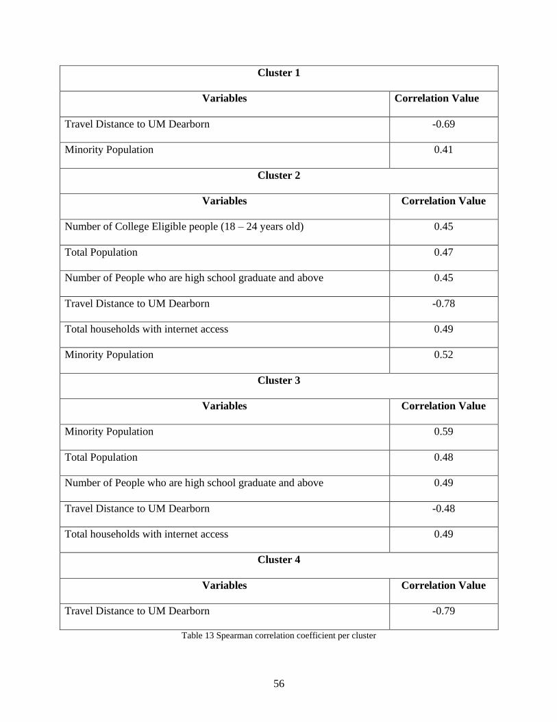
56

Cluster 1

Variables Correlation Value

Travel Distance to UM Dearborn -0.69


Cluster 2


Number of College Eligible people (18 – 24 years old) 0.45

Total Population 0.47



Total households with internet access 0.49


Cluster 3



Total Population 0.48



Total households with internet access 0.49

Cluster 4



Table 13 Spearman correlation coefficient per cluster

57

6.5 Control group analysis

In this study, two control groups were organized based on the number of students that each Zip

Code provides to the total population of the College of Engineering and Computer Science at UM-

Dearborn. A total of 269 Zip Codes are taken into account in this study. Control Group 1 included

the 27 Zip Codes (top 10 percent), with the highest enrollment count totaling 5828 students, and

Control Group 2 included the 54 Zip Codes (top 20 percent), which were home to 7259 students.

To compare the characteristics of the remaining Michigan Zip Codes with the two control groups,

a range was established for each factor comprising of lower and higher limits for respective Zip

Codes within each control group.

In the case of Control Group 1, 27 Zip Codes contribute 64.5% of the student population. The

common attributes of Zip Codes taken in this analysis are (1) Median household income, (2)

Number of Households with internet access, (3) College eligible population, (4) Travel Distance

to University, and (5) Number of people who are high school graduate and above, (6) Minority

Population, (7) Total Population.

The difference between the percentage of the students that come from these Zip Codes (from

control group 1) with the others is so significant and conclusive that it indicates these seven

variables, could be the most decisive to the number of students enrolling at UM-Dearborn. The

variable “Median household income” is used as an indicator of the purchasing power of the

population, the variable “Number of Households with internet access” is used as an indicator of

the level of coverage of the basic needs of the people, variable “Total Population” indicate the

population in that area and the factor “Number of people who are high school graduate and above”

indicates overall educational level in that particular area.

58

CONTROL GROUP 1

FACTORS

RANGE

Minimum Maximum

Median household

Income

25144

133040

Number of Households

with internet access

1523

21264

Number of College

Eligible people (18 – 24

years old)

931

14097

Travel Distance to

University (miles)

0

25.1

Number of People who

are high school graduate

and above

5227

62421

Minority Population 637

25947

Total Population 7554

67775

Table 14 Control group 1 range

In the next step, each Zip Code is compared to the characteristics of Control Group based on the

range of values of each factor (Table 14). The analysis shows that only 20 Zip Codes depicts

characteristics similar to Control Group 1. Out of the remaining 242 Zip Codes, 116 Zip Codes

show six similarities of seven possible (86%). And, only 42 Zip Codes show five similarities of

seven possible (71%). However, these similarities are not the same for every Zip Code. The only

commonalities detected were: (1) Number of households with internet access (2) Number of

People who are high school graduate and above. Now, in the case of Control Group 2, it comprises

of 54 Zip Codes with highest enrollment count that contribute 80% of the student population.

59

Out of the remaining 215 Zip Codes, 77 Zip Codes share all seven possible common characteristics

with Control Group 2 that are not shared by the other Zip Codes, and 88 Zip Codes show six

similarities of 7 possible (86%). The specific commonalities between these Zip Codes and control

group 2 were: (1) Total Population, (2) Number of households with internet access (3) Number of

College Eligible people, (4) Minority Population, and (5) Number of People who are high school

graduate and above.

Only 10 Zip Codes show five similarities of seven possible similarities (71%), and specific

commonalities shown were: (1) Median household income, (2) Number of households with

internet access (3) Number of People who are high school graduate and above.

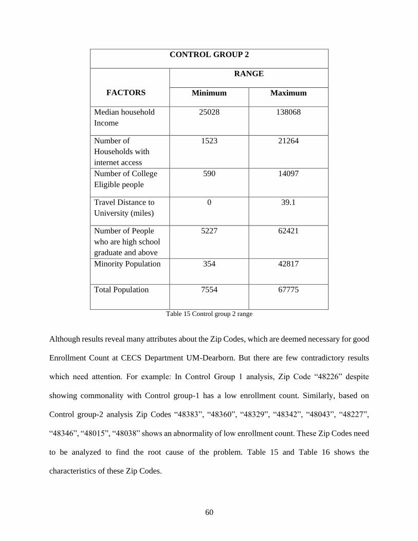
60

CONTROL GROUP 2

FACTORS

RANGE

Minimum Maximum

Median household

Income

25028

138068

Number of

Households with

internet access

1523

21264

Number of College

Eligible people

590

14097

Travel Distance to

University (miles)

0

39.1

Number of People

who are high school

graduate and above

5227

62421

Minority Population 354 42817

Total Population 7554 67775

Table 15 Control group 2 range

Although results reveal many attributes about the Zip Codes, which are deemed necessary for good

Enrollment Count at CECS Department UM-Dearborn. But there are few contradictory results

which need attention. For example: In Control Group 1 analysis, Zip Code “48226” despite

showing commonality with Control group-1 has a low enrollment count. Similarly, based on

Control group-2 analysis Zip Codes “48383”, “48360”, “48329”, “48342”, “48043”, “48227”,

“48346”, “48015”, “48038” shows an abnormality of low enrollment count. These Zip Codes need

to be analyzed to find the root cause of the problem. Table 15 and Table 16 shows the

characteristics of these Zip Codes.

61

Student

Counts

Zip

Codes

Median

household

Income

Number of

Households

with

internet

access

Number

of

College

Eligible

people

Travel

Distance

to

University

(miles)

Number of

People who

are high

school

graduate

and above

Minority

Population

Total

Populat

ion

1 48226 47894 2884 1144 13.8 5936 3818 6537

Table 16 Comparison to control group 1

Student

Counts

Zip

Codes

Median

household

Income

Number of

Households

with internet

access

Number

of College

Eligible

people

Travel

Distance

to

University

(miles)

Number of

People who

are high

school

graduate and

above

Minority

Population

Total

Populat

ion

4 48383 86333 4174 1273 37.3 12691 356 13544

1 48360 104389 3977 1230 38.1 11778 1217 12055

1 48329 70537 8479 2018 33 23023 2410 24917

1 48342 25989 4499 2323 28.3 13556 12426 17335

2 48043 39537 5075 1474 34.8 14106 5240 16383

4 48227 29971 7939 4618 8 35162 41528 42364

1 48346 74958

7911

2053

35.8

21498

1922

23067

4 48015

37958

2717

681

24.5

7129

2506

8299

3 48038 55567

16438

4103

34.9

39866

6507

43192

Table 17 Comparison to control group 2

62

Chapter 7. Discussion

This research addresses the issue of poor enrollment trends at the College of Engineering and

Computer Science department, University of Michigan-Dearborn. It assists University

administrators and policymakers to formulate strategies to attract and enroll more students at UM-

Dearborn.

The results could be helpful to recognize the economic limitations (such as access to basic needs,

median income.) that are faced by the students of specific Zip Codes/ communities and also

develop strategies such as community outreach programs.

Visual analysis using QGIS Maps led us to understand the distribution of various demographic

characteristics across Michigan and their effects on student’s admission. (Figure 5) shows the UM-

Dearborn CECS Undergraduate Enrollment Count of the year (2015 - 2019) from respective Zip

Codes. Also, the maximum representation of admitted students was from the southeast Michigan

area. (Figure 6 and Figure 7) show the educational level of People in the respective Zip Codes in

Michigan, which suggests that admitted students represented communities with diverse levels of

education. (Figure 8 and Figure 9) shows the Median Household Income of people and internet

access, respectively. These factors define the characteristics and provide the researchers with

additional insights and information about the social class, community characteristics, and the

lifestyle of admitted students on campus.

63

Further maps include the representation of Minority Population in the respective Zip Codes in

Michigan, Travel distance to UM-Dearborn from respective Zip Codes.

With a majority of the state’s industries and businesses, Southeast Michigan consists of more than

half of the state’s population. So, the large cluster of enrollment counts from this area is expected.

Thus, the GIS Mapping technique guided us to the different demographic factors which affect the

admission of students at the University of Michigan - Dearborn.

It is evident from the analysis that there are specific demographic attributes deemed necessary for

student’s enrollment decisions. These are (1) Minority Population in a Zip Code, (2) Number of

households with Internet access, (3) Travel Distance to UM-Dearborn, (4) Number of People who

are high school graduate and above, (5) Total Population, (6) Number of College Eligible people

(18 – 24 years old).

Furthermore, the results suggest opportunities for the university to provide support for current

students and advocate for support for pre-college students. Decision-makers should also take into

consideration Zip Codes such as “48226”, “48383”, “48360”, “48329”, “48342”, “48043”,

“48227”, “48346”, “48015”, “48038” which have an abnormality of low student enrollment count

despite achieving the highest level of performance in demographic characteristics that were

considered as significant (Figure 18).

64

Figure 18 Visualization of Zip Codes with similar characteristics to control groups

However, this study comprised only the Socioeconomic and Demographic Factors for the analysis

of enrollment trends. More personal (e.g., specific racial characteristics vs. minority groups) and

academic factors can be considered to investigate the relationship of such factors on college

enrollments and the academic success of students. Also, some Zip Codes that are not considered

in this study due to unavailability of data from US Census are “41010”, “46411”, “48153”,

“48333”, “49696”, “48303”.

65

Chapter 8. Conclusion

The issue of whether or not the Socioeconomic and Demographic Factors of a neighborhood

influence youngsters’ educational attainment has a lot of policy relevance. If these factors are

significant, then policies that exclusively emphasize on building up people’s skills based on

academic factors without dealing with their demographic factors are probably not going to be

effective in increasing educational attainment.

This project aims at predicting student enrollment trends based on demographic characteristics of

their home Zip Codes and determine those characteristics that influence the possibility of student’s

enrollment in CECS at the University of Michigan- Dearborn. Furthermore, these results will be

utilized for making strategies to attract, engage, and retain more students.

Based on this research, addressing the issue of poor enrollment suggests more consideration should

be given to the surroundings in which youngsters live.

66

Chapter 9. Future work

This study was designed and performed only for students at the College of Engineering and

Computer science at the University of Michigan- Dearborn. The results from the analysis of the

data in this research indicate that such a study, when performed at a larger scale, has the potential

to uncover existing pathways to engineering degrees used by URM students (Underrepresented

Minorities).

Additionally, we may find unexplored opportunities and pathways to engage, admit, and enroll

more historically underrepresented students from communities with low enrollment trends. This

work can encourage partnerships that can drive institutional initiatives, k-12 educational policy,

research, and curricular changes that lead to more significant support and success for minority

youth in engineering.

Also, this study comprised only the demographic factors for the analysis of enrollment trends.

More personal and academic factors can be taken into account to investigate the relationship of

such factors on college enrollments and also the academic success of students. In the next phase

of the study, undergraduate engineering student data over multiple years can be taken into account.

The factors that can be included in further large scale study are (1) Student Race/Ethnicity, (2)

Student - Aid eligibility (PELL), (3) gender (GENDER), (4) FTIAC/TRANSFER Status, (5)

anticipated graduation date, (6) High school Zip Code, (7) Personal Zip Code, (8) Student AP/IB

or similar Courses completed, (9) Student AP courses available at the High school, (10) Graduation

rates in 4,5, 6+ years by race and gender, (11) Student retention rates by race,

67

(12) High school grade point average (HSGPA), (13) SAT math score (SATQ), (14) SAT verbal

score (SATV), (15) Student’s first semester GPA, (16) Poverty index, (17) Access to basic needs

(Access to internet, power, technology). Furthermore, with the use of statistical techniques, we

hope to identify factors, trends, and opportunities to positively impact the academic success of

students and also increase enrollment counts, especially for underrepresented minorities.

68

References

Adelman, C. (1998). Women and Men of the Engineering Path: A Model for Analyses of

Undergraduate Careers. National Inst. on Postsecondary Education, Libraries, and

Lifelong Learning (ED/OERI), Washington, DC.; National Science Foundation,

Arlington, VA.

Alexander, N., Moyeed, R., & Stander, J. (2000). Spatial modelling of individual-level parasite

counts using the negative binomial distribution. Biostatistics, 1, 453–463.

Alm, J., & Winters, J. V. (2009). Distance and intrastate college student migration. Economics of

Education Review, 28, 728-738.

Andres, L., & Carpenter, S. (1997). Today's Higher Education Students: Issues of Admission,

Retention, Transfer, and Attrition in Relation to Changing Student

Demographics. https://eric.ed.gov/?id=ED444638

Arzú, D. V. M., & Valle, C. M. C. (2018). The socio-economic characteristics of the hometowns

of the students. IEEE Global Engineering, 779-786.

Astin, A. W., & Astin, H. S. (1992). Undergraduate Science Education: The Impact of Different

College Environments on the Educational Pipeline in the Sciences. Final

Report. https://eric.ed.gov/?id=ED362404

Attfield, I., Tamiru, M., Parolin, B., & De Grauwe, A. (2002). Improving Micro-Planning in

Education through a Geographical Information System: Studies on Ethiopia and

Palestine. School Mapping and Local-Level Planning. United Nations Educational,

Scientific, and Cultural Organization, Paris (France). International Inst. for Educational

Planning.

Bahr, P. R. (2013). Classifying Community Colleges Based on Students’ Patterns of Use Research

in Higher Education, 433 – 460.

Bargh, J. A., & McKenna, K. Y. A. (2004). The Internet and Social Life. Annual Review of

Psychology, 55, 573 -590.

Bartik, T., Hershbein, B., & Lachowska, M. (2017). The Effects of the Kalamazoo Promise

Scholarship on College Enrollment, Persistence, and

Completion. https://papers.ssrn.com/sol3/papers.cfm?abstract_id=2624727

Belley, P., & Lochner, L. (2007). The Changing Role of Family Income and Ability in

Determining Educational Achievement Journal of Human Capital, 1, 37-89.

Boveng, P., Bengtson, J. L., Withrow, D., Cesarone, J. C., & Simpkins, M. (2003). The

Abundance of Harbor Seals in the Gulf of Alaska Marine Mammal Science, 19(1), 111-

127.

https://eric.ed.gov/?id=ED444638


https://papers.ssrn.com/sol3/papers.cfm?abstract_id=2624727

69

Bressers, B., & Bergen, L. (2002). Few university students reading newspapers

online. Newspaper Research Journal, 23, 32- 45.

Brey, C. d., Musu, L., McFarland, J., Wilkinson-Flicker, S., Diliberti, M., Zhang, A., Branstetter,

C., & Wang, X. (2019). Status and Trends in the Education of Racial and Ethnic Groups

2018. https://eric.ed.gov/?id=ED592833

Brody, G. H., Kogan, S. M., & Grange, C. M. (2012). Translating Longitudinal, Developmental

Research with Rural African American Families into Prevention

Programs for Rural African American Youth. American Psychological Association, 551–

568.

Canedo, V. B., Noelia Sánchez, & Betanzos, A. A. (2013). A review of feature selection methods

on synthetic data. Knowledge and Information Systems, 34, 483 – 519.

Castleman, B. L., & Long, B. T. (2016). Looking beyond Enrollment: The Causal Effect of Need-

Based Grants on College Access, Persistence, and Graduation. Journal of Labor

Economics, 34, 1023-1073.

Chen, E., & Miller, G. E. (2013). Socioeconomic Status and Health: Mediating and Moderating

Factors Annual Review of Clinical Psychological Review of Clinical Psychology, 9.

Chen, E., Miller, G. E., Brody, G. H., & Lei, M. (2014). Neighborhood Poverty, College

Attendance, and Diverging Profiles of Substance Use and Allostatic Load inRural African

American Youth Clinical Psychological Science, 3(5), 675–685.

Chen, X., & Soldner, M. (2013). STEM Attrition: College Students' Paths into and out of STEM

Fields. Statistical Analysis Report. https://files.eric.ed.gov/fulltext/ED544470.pdf

Clinedinst, M., Anna-Marianicola, Tara. (2015). State of college

admission. https://www.nacacnet.org/globalassets/documents/publications/research/2015

soca.pdf

Cohen, C. C. D., & Deterding, N. (2013). Widening the Net: National Estimates of Gender

Disparities in Engineering. Journal of Engineering Education, 211-226.

Cotten, S. R., & Jelenewicz, S. M. (2006). A Disappearing Digital Divide Among College

Students? Social Science Computer Review, 24(4), 497-506.

Daoud, J. I. (2017). Multicollinearity and Regression Analysis Journal of Physics: Conference

Series, https://iopscience.iop.org/article/10.1088/1742-6596/949/1/012009/meta

Dare, A., Dare, L., & Nowicki, E. (2017). Concurrent enrollment: comparing how educators and

students categorize students’ motivations. Social Psychology of Education, 20, 195 – 213.


https://files.eric.ed.gov/fulltext/ED544470.pdf

https://www.nacacnet.org/globalassets/documents/publications/research/2015soca.pdf

https://www.nacacnet.org/globalassets/documents/publications/research/2015soca.pdf

70

Do, C. (2004). The effects of local colleges on the quality of college attended Economics of

Education Review, 23(3), 249-257.

Doyle, W. R., & Skinner, B. T. (2017). Predicting Postsecondary Attendance by Income in the

American States Using Multilevel Regression with Poststratificatio. SSRN.

Eagan, K., Stolzenberg, E. B., Bates, A. K., Aragon, M. C., Suchard, M. R., & Rios-Aguilar, C.

(2015). The American freshman: National norms fall

2015. https://www.heri.ucla.edu/monographs/TheAmericanFreshman2015-

Expanded.pdf

ERAY, O. (2012). Application of Geographic Information System (GIS) in Education. Journal of

Technical Science and Technologies, 53-58.

Ethington, C. A. (1990). A psychological model of student persistence. Research in Higher

Education, 279 – 293.

Fairlie, R. W., London, R. A., Rosner, R., & Pastor, M. (2006). Crossing the Divide

Immigrant Youth and

Digital Disparity in California. https://cjtc.ucsc.edu/docs/digital.pdf

File, T., & Ryan, C. (2014). Computer and Internet Use in the United States:

2013. https://selectra.co.uk/sites/default/files/pdf/computerandinternetuse.pdf

Fortson, B. L. S., Joseph R.Chen, Yi-Chuen, Malone, J., & Ben, K. S. D. (2010). Internet Use,

Abuse, and Dependence Among Students at a Southeastern Regional University Journal

of American College Health, 56(2), 137-144.

Griffith, A. L., & Rothstein, D. S. (2009). Can’t get there from here: The decision to apply to a

selective college. Economics of Education Review, 620-628.

Harding, D. J. (2003). Counterfactual Models of Neighborhood Effects: The Effect

of Neighborhood Poverty on Dropping Out and Teenage Pregnancy 1. American Journal

of Sociology 9, 676-719.

Hartman, H., & Hartman, M. (2006). Leaving Engineering: Lessons from Rowan University’s

College of Engineering Journal of Engineering Education, 95(1), 49-61.

Heller, D. E. (2006). Merit Aid and College Access. Symposium on the Consequences of Merit-

Based Student Aid.

Heller, D. E., & Marin, P. (2002). Who Should We Help? The Negative Social Consequences of

Merit Scholarships. https://eric.ed.gov/?id=ED468845

Hillman, N., & Wetchman, T. (2016). Education deserts: the continued significance of 'place' in

the twenty-first century. American Council on Education.

https://www.heri.ucla.edu/monographs/TheAmericanFreshman2015-Expanded.pdf

https://www.heri.ucla.edu/monographs/TheAmericanFreshman2015-Expanded.pdf

https://cjtc.ucsc.edu/docs/digital.pdf

https://selectra.co.uk/sites/default/files/pdf/computerandinternetuse.pdf


71

Hocking, R. R., & Pendleton, O. J. (1983). The regression dilemma. Communications in Statistics

- Theory and Methods, 12(5), 497-527.

Hodgkinson, H. (2000). An interview with Harold Hodgkinson: Demographics--ignore them at

your

peril [Interview]. https://www.jstor.org/stable/20439886?seq=1#metadata_info_tab_cont

ents

Hodgkinson, H. (2001). Educational Demographics: What Teachers Should Know. Educational

Leadership, 58.

Hogrebe, M. C., Blankson, L. K., & Zou, L. (2008). Examining Regional Science Attainment and

School–Teacher Resources Using GIS Education and Urban Society, 40, 570–589.

Horrigan, J. B., & Duggan, M. (2015). Home Broadband

2015. https://www.pewresearch.org/internet/wp-

content/uploads/sites/9/2015/12/Broadband-adoption-full.pdf

Hybels, C. F. B., Dan G., Pieper, C. F. L., Lawrence R., & Steffens, D. C. (2009). Profiles of

Depressive Symptoms in Older Adults Diagnosed with Major Depression: Latent Cluster

Analysis. The American Journal of Geriatric Psychiatry, 387-396.

Jackson, L. A., & Ervin, K. S. G., Philip D.Schmitt, Neal. (2001). Gender and the Internet: Women

Communicating and Men Searching Sex Roles, 44, 363 – 379.

Jackson, L. A. E., Alexander vonBiocca, Frank A.Barbatsis, Gretchen Zhao, Yong, & Fitzgerald,

H. E. (2006). Does Home Internet Use Influence the Academic Performance of

Low-Income Children? Developmental Psychology, 42, 429–435.

Jennings, P. J. (2008). Using Cluster Analysis to Define Geographical Rating Territories Casualty

Actuarial Society, 34-52.

Jensen, D. R. R., D. E. (2013). Revision: Variance Inflation in Regression. Advances in Decision

Sciences, 15.

Jones, S., Johnson, C., & Millermaier, S. e., Francisco Seoane. (2009). U.S. College Students’

Internet Use: Race, Gender and Digital Divides Journal of Computer-Mediated

Communication, 14(2), 244–264.

Kaufman, L., & Rousseeuw, P. J. (2009). Finding Groups in Data: An Introduction to Cluster

Analysis. John Wiley & Sons.

Kerski, J. J. (2007). The Implementation and Effectiveness of Geographic Information Systems

Technology and

Methods in Secondary Education. Journal of Geography, 102, 128-137.

https://www.jstor.org/stable/20439886?seq=1#metadata_info_tab_contents

https://www.jstor.org/stable/20439886?seq=1#metadata_info_tab_contents

https://www.pewresearch.org/internet/wp-content/uploads/sites/9/2015/12/Broadband-adoption-full.pdf

https://www.pewresearch.org/internet/wp-content/uploads/sites/9/2015/12/Broadband-adoption-full.pdf

72

Kinsler, J., & Pavan, R. (2011). Family income and higher education choices: The importance of

accounting for college quality. Journal of human capital, 5, 453-477.

Kumar, V., & Minz, S. (2014). Feature Selection: A literature Review. Smart Computing

Review 4, 211-229.

Lerner, R. M., & Steinberg, L. (2004). The scientific study of adolescent development. John Wiley

& Sons.

Lin, D., Foster, D. P., & Ungar, L. H. (2011). VIF Regression: A Fast Regression Algorithm for

Large Data Journal of the American Statistical Association, 106(493), 232-247.

Liu, H., & Yu, L. (2005). Toward integrating feature selection algorithms for classification and

clustering. IEEE Transactions on Knowledge and Data Engineering, 17(4), 491-502.

Lord, S. M. C., Michelle Madsen, Layton Richard A.Long, Russell A., Ohland, M. W., &

Wasburn, M. H. (2009). Who’s Persisting in Engineering? A Comparative Analysis of

Female and Male Asian, Black, Hispanic, Native American, and White Students. Journal

of Women and Minorities in Science and Engineering, 15(2), 167-190.

M C Millan, S. J., & Morrison, M. (2006). Coming of age with the internet: A qualitative

exploration of how the internet has become an integral part of young people’s lives. new

media & society, 8(1), 73–95.

Ma, Y. (2009). Family Socioeconomic Status, Parental Involvement, and College Major

Choices—Gender, Race/Ethnic, and Nativity Patterns. Sociological Perspectives, 52(2),

211–234.

McDonald, J. H. (2015). Spearman Rank Correlation. S parky House Publishing

Milliken, G. A., & Johnson, D. E. (2002). Analysis of Messy data. Chapman & Hall/CRC.

Moore, R., Vitale, D., & Stawinoga, N. (2018). The digital divide and educational equity (Insights

in Education and Work, Issue. https://files.eric.ed.gov/fulltext/ED593163.pdf

Ness, E. C., & Tucker, R. (2008). Eligibility Effects on College Access: Under-represented

Student Perceptions of Tennessee’s Merit Aid Program Research in Higher

Education 49, 569-588.

Ng, K., & Liu, H. (2000). Customer Retention via Data Mining. Artificial Intelligence Review,

14, 569 – 590.

Nichols, A. H. (2015). The Pell Partnership: Ensuring a Shared Responsibility for Low-Income

Student Success. https://eric.ed.gov/?id=ED566658

https://files.eric.ed.gov/fulltext/ED593163.pdf


73

Norman, E. (2013). The Impact of Demographics on 21st Century Education. Society, 50, 272 –

282.

O'Neill, R., & Wetherill, G. B. (1971). The Present State of Multiple Comparison

Methods Journal of the Royal Statistical Society. Series B (Methodological), 33, 218-250.

Odell, P. M. K., Kathleen O., Schumacher, P., & Delucchi, M. (2004). Internet Use Among

Female and Male College Students. CyberPsychology & Behavior, 3(5), 855-862.

Ohland, M., W. Brawner, C. E., Camacho, M. M., Layton, R. A., Long, R. A., Lord, S. M., &

Wasburn, M. H. (2011). Race, Gender, and Measures of Success in Engineering

Education. Journal of Engineering Education, 100(2), 225-252.

Osborne, J. W., & Waters, E. (2002). Four assumptions of multiple regression that researchers

should always test. Practical Assessment, Research, and Evaluation 8(2).

Ovink, S. M., & Kalogrides, D. (2015). No place like home? Familism and Latino/a–white

differences in college pathways Social Science Research, 219-235.

Pluhta, E. A., & Penny, G. R. (2013). The Effect of a Community College Promise Scholarship

on Access and Success Community College Journal of Research and Practice, 37, 723-

734.

Pruijt, H. (2002). Social Capital and the Equalizing Potential of the Internet Social Science

Computer Review 20(2), 109–115.

Pérez, P. A., & McDonough, P. M. (2008). Understanding Latina and Latino College Choice: A

Social Capital and Chain Migration Analysis. Journal of Hispanic Higher Education 7(3),

249–265.

Ratledge, A., O'Donoghue, R., Cullinan, D., & Camo-Biogradlija, J. (2019). A Path from Access

to Success: Interim Findings from the Detroit Promise Path

Evaluation. https://eric.ed.gov/?id=ED594432

Robert, T., Walther, G., & Hastie, T. (2001). Estimating the number of clusters in a data set via

the gap statistic. Royal Statistical Society, 63(2), 411-423.

Romesburg, H. C. (2004). Cluster analysis for researchers. Lulu Press.

Saenz, V. B. H., DerylBukoski, Beth E., & Kim, S., Kye-hyoungValdez, Patrick. (2011).

Community College Student Engagement Patterns: A Typology Revealed Through

Exploratory Cluster Analysis Community College Review, 39(3), 235–267.

Shaw, E. J., Kobrin, J. L., Packman, S. F., & Schmidt, A. E. (2009). Describing Students Involved

in the Search Phase of the College Choice Process: Journal of Advanced Academics 20(4),

662–700.


74

Stewart, E. B. S., Eric A.Simons, Ronald L. (2007). The Effect of Neighborhood Context on the

College Aspirations of African American Adolescents. American Educational Research

Journal, 44(4), 896–919.

Tibshirani, R. (1996). Regression Shrinkage and Selection Via the Lasso. Journal of the Royal

Statistical Society: Series B (Methodological), 58(1), 267-288.

Tinto, V. (1987). Leaving College: Rethinking the Causes and Cures of Student Attrition.

Tukey, J. W. (1949). Comparing Individual Means in The Analysis of Variance Biometrics, 5(2),

99-114.

VanderStel, A. (2014). The Impact of Demographics in Education. Undergraduate Research and

Creative Practice.

Venegas, K. M. (2007). The Internet and College Access: Challenges for Low-Income Students

American Academic, 3, 141-154.

Volman, M., Edith vanHeemskerk, IrmaKuiper, Els. (2005). New technologies, new differences.

Gender and ethnic differences in pupils’ use of ICT in primary and secondary

education. Computers & Education, 45(1), 35-55.

Wilcox, L. B. (2008). Is there a Correlation between the Digital Divide and College Access?

Wills, T. A., & Pokhrel, P. M., EllenFenster, Bonnie. (2011). Behavioral and Emotional

Regulation and Adolescent Substance Use Problems: A Test of Moderation Effects in a

Dual-Process Model American Psychological Association .25(2), 279–292.

Xing, E. P., Jordan, M. I., & Karp, R. M. (2001). Feature Selection for High-Dimensional

Genomic Microarray Data.

Yang, S., Gilbert. (2015). Negative Binomial Regression. The Southwest Respiratory and Critical

Care Chronicles 3(10), 50-53.

Yu, L., & Liu, H. (2003). Feature Selection for High-Dimensional Data: A Fast Correlation-Based

Filter Solution. Proceedings of the Twentieth International Conference on Machine

Learning (ICML-2003).

Zhang, Y. (2004). Comparison of Internet Attitudes between Industrial Employees and College

Students CyberPsychology & Behavior, 5(2), 143-149.

College Enrollment Trends and Pattern Evaluation

Documents

Transcript of College Enrollment Trends and Pattern Evaluation