Asma B ancode C atalu ñ a Admitimos órdenes de suscripción ...
Upload
khangminh22Category
view
2download
0
Ordinary di�erential equations
and
Dynamical Systems
Gerald Teschl
Gerald Teschl
Institut f�ur Mathematik
Strudlhofgasse 4
Universit�at Wien
1090 Wien, Austria
E-mail: [email protected]
URL: http://www.mat.univie.ac.at/~gerald/
1991 Mathematics subject classi�cation. 34-01
Abstract. This manuscript provides an introduction to ordinary di�erential
equations and dynamical systems. We start with some simple examples
of explicitly solvable equations. Then we prove the fundamental results
concerning the initial value problem: existence, uniqueness, extensibility,
dependence on initial conditions. Furthermore we consider linear equations,
the Floquet theorem, and the autonomous linear ow.
Then we establish the Frobenius method for linear equations in the com-
plex domain and investigates Sturm{Liouville type boundary value problems
including oscillation theory.
Next we introduce the concept of a dynamical system and discuss sta-
bility including the stable manifold and the Hartman{Grobman theorem for
both continuous and discrete systems.
We prove the Poincar�e{Bendixson theorem and investigate several ex-
amples of planar systems from classical mechanics, ecology, and electrical
engineering. Moreover, attractors, Hamiltonian systems, the KAM theorem,
and periodic solutions are discussed as well.
Finally, there is an introduction to chaos. Beginning with the basics for
iterated interval maps and ending with the Smale{Birkho� theorem and the
Melnikov method for homoclinic orbits.
Keywords and phrases. Ordinary di�erential equations, dynamical systems,
Sturm-Liouville equations.
Typeset by AMS-LATEX and Makeindex.
Version: December 17, 2001
Copyright c October 2001 by Gerald Teschl


Contents
Preface vii
Part 1. Classical theory
Chapter 1. Introduction 3
x1.1. Newton's equations 3
x1.2. Classi�cation of di�erential equations 5
x1.3. First order equations 8
x1.4. Finding explicit solutions 11
Chapter 2. Initial value problems 17
x2.1. Fixed point theorems 17
x2.2. The basic existence and uniqueness result 19
x2.3. Dependence on the initial condition 22
x2.4. Extensibility of solutions 25
x2.5. Euler's method and the Peano theorem 27
x2.6. Appendix: Volterra integral equations 30
Chapter 3. Linear equations 35
x3.1. Preliminaries from linear algebra 35
x3.2. Linear �rst order systems 41
x3.3. Periodic linear systems 45
x3.4. Linear autonomous �rst order systems 49
Chapter 4. Di�erential equations in the complex domain 53
iii

iv Contents
x4.1. The basic existence and uniqueness result 53
x4.2. Linear equations 55
x4.3. The Frobenius method 59
x4.4. Second order equations 62
Chapter 5. Boundary value problems 69
x5.1. Introduction 69
x5.2. Symmetric compact operators 72
x5.3. Regular Sturm-Liouville problems 76
x5.4. Oscillation theory 81
Part 2. Dynamical systems
Chapter 6. Dynamical systems 89
x6.1. Dynamical systems 89
x6.2. The ow of an autonomous equation 90
x6.3. Orbits and invariant sets 93
x6.4. Stability of �xed points 97
x6.5. Stability via Liapunov's method 99
x6.6. Newton's equation in one dimension 100
Chapter 7. Local behavior near �xed points 105
x7.1. Stability of linear systems 105
x7.2. Stable and unstable manifolds 107
x7.3. The Hartman-Grobman theorem 113
x7.4. Appendix: Hammerstein integral equations 117
Chapter 8. Planar dynamical systems 119
x8.1. The Poincar�e{Bendixson theorem 119
x8.2. Examples from ecology 123
x8.3. Examples from electrical engineering 127
Chapter 9. Higher dimensional dynamical systems 133
x9.1. Attracting sets 133
x9.2. The Lorenz equation 136
x9.3. Hamiltonian mechanics 140
x9.4. Completely integrable Hamiltonian systems 144
x9.5. The Kepler problem 149
x9.6. The KAM theorem 150

Contents v
Part 3. Chaos
Chapter 10. Discrete dynamical systems 157
x10.1. The logistic equation 157
x10.2. Fixed and periodic points 160
x10.3. Linear di�erence equations 162
x10.4. Local behavior near �xed points 164
Chapter 11. Periodic solutions 167
x11.1. Stability of periodic solutions 167
x11.2. The Poincar�e map 168
x11.3. Stable and unstable manifolds 170
x11.4. Melnikov's method for autonomous perturbations 173
x11.5. Melnikov's method for nonautonomous perturbations 178
Chapter 12. Discrete dynamical systems in one dimension 181
x12.1. Period doubling 181
x12.2. Sarkovskii's theorem 184
x12.3. On the de�nition of chaos 185
x12.4. Cantor sets and the tent map 188
x12.5. Symbolic dynamics 191
x12.6. Strange attractors/repellors and fractal sets 195
x12.7. Homoclinic orbits as source for chaos 199
Chapter 13. Chaos in higher dimensional systems 203
x13.1. The Smale horseshoe 203
x13.2. The Smale-Birkho� homoclinic theorem 205
x13.3. Melnikov's method for homoclinic orbits 206
Bibliography 211
Glossary of notations 213
Index 215


Preface
The present manuscript constitutes the lecture notes for my courses Ordi-
nary Di�erential Equations and Dynamical Systems and Chaos held at the
University of Vienna in Summer 2000 (5hrs.) and Winter 2000/01 (3hrs),
respectively.
It is supposed to give a self contained introduction to the �eld of ordi-
nary di�erential equations with emphasize on the view point of dynamical
systems. It only requires some basic knowledge from calculus, complex func-
tions, and linear algebra which should be covered in the usual courses. I tried
to show how a computer system, Mathematica, can help with the investiga-
tion of di�erential equations. However, any other program can be used as
well.
The manuscript is available from
http://www.mat.univie.ac.at/~gerald/ftp/book-ode/
Acknowledgments
I wish to thank my students P. Capka and F. Wisser who have pointed
out several typos and made useful suggestions for improvements.
Gerald Teschl
Vienna, Austria
May, 2001
vii


Part 1
Classical theory


Chapter 1
Introduction
1.1. Newton's equations
Let us begin with an example from physics. In classical mechanics a particle
is described by a point in space whose location is given by a function
x : R ! R3: (1.1)
The derivative of this function with respect to time is the velocity
v = _x : R ! R3 (1.2)
of the particle and the derivative of the velocity is called acceleration
a = _v : R ! R3: (1.3)
In such a model the particle is usually moving in an external force �eld
F : R3 ! R3 (1.4)
describing the force F (x) acting on the particle at x. The basic law of
Newton states that at each point x in space the force acting on the particle
must be equal to the acceleration times the mass m > 0 of the particle, that
is,
m �x(t) = F (x(t)); for all t 2 R: (1.5)
Such a relation between a function x and its derivatives is called a di�er-
ential equation. Equation (1.5) is called of second order since the highest
derivative is of second degree. More precisely, we even have a system of
di�erential equations since there is one for each coordinate direction.
In our case x is called the dependent and t is called the independent
variable. It is also possible to increase the number of dependent variables
3
4 1. Introduction
by considering (x; v). The advantage is that we now have a �rst order system
_x(t) = v(t)
_v(t) =1
mF (x(t)): (1.6)
This form is often better suited for theoretical investigations.
For given force F one wants to �nd solutions, that is functions x(t) which
satisfy (1.5) (respectively (1.6)). To become more speci�c, let us look at the
motion of a stone falling towards the earth. In the vicinity of the surface
of the earth, the gravitational force acting on the stone is approximately
constant and given by
F (x) = �mg
0@ 0
0
1
1A : (1.7)
Here g is a positive constant and the x3 direction is assumed to be normal
to the surface. Hence our system of di�erential equations reads
m �x1 = 0;
m �x2 = 0;
m �x3 = �mg: (1.8)
The �rst equation can be integrated with respect to t twice, resulting in
x1(t) = C1 + C2t, where C1, C2 are the integration constants. Computing
the values of x1, _x1 at t = 0 shows C1 = x1(0), C2 = v1(0), respectively.
Proceeding analogously with the remaining two equations we end up with
x(t) = x(0) + v(0) t� g
2
0@ 0
0
1
1A t
2: (1.9)
Hence the entire fate (past and future) of our particle is uniquely determined
by specifying the initial location x(0) together with the initial velocity v(0).
From this example you might get the impression, that solutions of di�er-
ential equations can always be found by straightforward integration. How-
ever, this is not the case in general. The reason why it worked here is,
that the force is independent of x. If we re�ne our model and take the real
gravitational force
F (x) = �m x
jxj3 ; (1.10)
1.2. Classi�cation of di�erential equations 5
our di�erential equation reads
m �x1 = � m x1
(x21 + x22 + x23)3=2
;
m �x2 = � m x2
(x21 + x22 + x23)3=2
;
m �x3 = � m x3
(x21 + x22 + x
23)3=2
(1.11)
and it is no longer clear how to solve it. Moreover, it is even unclear whether
solutions exist at all! (We will return to this problem in Section 9.5.)
Problem 1.1. Consider the case of a stone dropped from the height h.
Denote by r the distance of the stone from the surface. The initial condition
reads r(0) = h, _r(0) = 0. The equation of motion reads
�r = � M
(R+ r)2(exact model) (1.12)
respectively
�r = �g (approximate model); (1.13)
where g = M=R2 and R, M are the radius, mass of the earth, respectively.
(i) Transform both equations into a �rst order system.
(ii) Compute the solution to the approximate system corresponding to
the given initial condition. Compute the time it takes for the stone
to hit the surface (r = 0).
(iii) Assume that the exact equation has also a unique solution corre-
sponding to the given initial condition. What can you say about
the time it takes for the stone to hit the surface in comparison
to the approximate model? Will it be longer or shorter? Estimate
the di�erence between the solutions in the exact and in the approx-
imate case. (Hints: You should not compute the solution to the
exact equation! Look at the minimum, maximum of the force.)
(iv) Grab your physics book from high school and give numerical values
for the case h = 10m.
1.2. Classi�cation of di�erential equations
Let U � Rm , V � R
n and k 2 N0 . Then Ck(U; V ) denotes the set of
functions U ! V who have continuous derivatives up to order k. In addition,
we will abbreviate C(U; V ) = C0(U; V ) and Ck(U) = C
k(U;R).
A classical ordinary di�erential equation (ODE) is a relation of the
form
F (t; x; x(1); : : : ; x(k)) = 0 (1.14)
6 1. Introduction
for the unknown function x 2 Ck(R). Here F 2 C(U) with U an open
subset of Rk+2 and
x(k)(t) =
dkx(t)
dtk; k 2 N0 ; (1.15)
are the ordinary derivatives of x. One frequently calls t the independent
and x the dependent variable. The highest derivative appearing in F is
called the order of the di�erential equation. A solution of the ODE (1.14)
is a function � 2 Ck(I), where I is an interval, such that
F (t; �(t); �(1)(t); : : : ; �(k)(t)) = 0; for all t 2 I: (1.16)
This implicitly implies (t; �(t); �(1)(t); : : : ; �(k)(t)) 2 U for all t 2 I.Unfortunately there is not too much one can say about di�erential equa-
tions in the above form (1.14). Hence we will assume that one can solve F
for the highest derivative resulting in a di�erential equation of the form
x(k) = f(t; x; x(1); : : : ; x(k�1)): (1.17)
This is the type of di�erential equations we will from now on look at.
We have seen in the previous section that the case of real-valued func-
tions is not enough and we should admit the case x : Rn ! R. This leads
us to systems of ordinary di�erential equations
x(k)1 = f1(t; x; x
(1); : : : ; x
(k�1));
...
x(k)n = fn(t; x; x
(1); : : : ; x
(k�1)): (1.18)
Such a system is said to be linear, if it is of the form
x(k)i = gi(t) +
nXl=1
k�1Xj=0
fi;j;l(t)x(j)l : (1.19)
It is called homogeneous, if gi(t) = 0.
Moreover, any system can always be reduced to a �rst order system by
changing to the new set of independent variables y = (x; x(1); : : : ; x(k�1)).
This yields the new �rst order system
_y1 = y2;
...
_yk�1 = yk;
_yk = f(t; y): (1.20)

1.2. Classi�cation of di�erential equations 7
We can even add t to the independent variables z = (t; y), making the right
hand side independent of t
_z1 = 1;
_z2 = z3;
...
_zk = zk+1;
_zk+1 = f(z): (1.21)
Such a system, where f does not depend on t, is called autonomous. In
particular, it suÆces to consider the case of autonomous �rst order systems
which we will frequently do.
Of course, we could also look at the case t 2 Rm implying that we have
to deal with partial derivatives. We then enter the realm of partial dif-
ferential equations (PDE). However, this case is much more complicated
and is not part of this manuscript.
Finally note that we could admit complex values for the dependent vari-
ables. It will make no di�erence in the sequel whether we use real or complex
dependent variables. However, we will state most results only for the real
case and leave the obvious changes to the reader. On the other hand, the
case where the independent variable t is complex requires more then obvious
modi�cations and will be considered in Chapter 4.
Problem 1.2. Classify the following di�erential equations.
(i) y0(x) + y(x) = 0.
(ii) d2
dt2u(t) = sin(u(t)).
(iii) y(t)2 + 2y(t) = 0.
(iv) @2
@x2u(x; y) + @2
@y2u(x; y) = 0.
Problem 1.3. Which of the following di�erential equations are linear?
(i) y0(x) = sin(x)y + cos(y).
(ii) y0(x) = sin(y)x+ cos(x).
(iii) y0(x) = sin(x)y + cos(x).
Problem 1.4. Find the most general form of a second order linear equation.
Problem 1.5. Transform the following di�erential equations into �rst order
systems.
(i) �x+ t sin( _x) = x.
(ii) �x = �y, �y = x.

8 1. Introduction
The last system is linear. Is the corresponding �rst order system also linear?
Is this always the case?
Problem 1.6. Transform the following di�erential equations into autonomous
�rst order systems.
(i) �x+ t sin( _x) = x.
(ii) �x = � cos(t)x.
The last equation is linear. Is the corresponding autonomous system also
linear?
1.3. First order equations
Let us look at the simplest (nontrivial) case of a �rst order autonomous
equation
_x = f(x); x(0) = x0; f 2 C(R): (1.22)
This equation can be solved using a small ruse. If f(x0) 6= 0, we can divide
both sides by f(x) and integrate both sides with respect to t,Z x
x0
dy
f(y)= t; (1.23)
to obtain an implicit form of the solution. Moreover, since the function
F (x) =R xx0f(y)�1dy is strictly monotone, it can be inverted and we obtain
the solution
�(t) = F�1(t); �(0) = F
�1(0) = x0; (1.24)
of our initial value problem. Moreover, if f(x) > 0 for x 2 (x1; x2) (the case
f(x) < 0 follows by replacing x! �x), we can de�ne
T+ = F (x2) 2 (0;1]; respectively T� = F (x1) 2 [�1; 0): (1.25)
Then � 2 C1((T�; T+)) and
limt"T+
�(t) = x2; respectively limt#T
�
�(t) = x1: (1.26)
In particular, � exists for all t > 0 (resp. t < 0) if and only if 1=f(x) is not
integrable near x2 (resp. x1). Now let us look at some examples. If f(x) = x
we have (x1; x2) = (0;1) and
F (x) = ln(x
x0): (1.27)
Hence T� = �1 and
�(t) = x0et: (1.28)
Thus the solution is globally de�ned for all t 2 R. Next, let f(x) = x2. We
have (x1; x2) = (0;1) and
F (x) =1
x0� 1
x: (1.29)
1.3. First order equations 9
Hence T+ = 1=x0, T� = �1 and
�(t) =x0
1� x0t: (1.30)
In particular, the solution is no longer de�ned for all t 2 R. Moreover, since
limt"1=x0 �(t) =1, there is no way we can possibly extend this solution for
t � T+.
Now what is so special about the zeros of f(x)? Clearly, if f(x1) = 0,
there is a trivial solution
�(t) = x1 (1.31)
to the initial condition x(0) = x1. But is this the only one? If we haveZ x0
x1
dy
f(y)<1; (1.32)
then there is another solution
'(t) = F�1(t); F (x) =
Z x
x1
dy
f(y)(1.33)
with '(0) = x1 which is di�erent from �(t)!
For example, consider f(x) =pjxj, then (x1; x2) = (0;1),
F (x) = 2(px�px0): (1.34)
and
�(t) = (px0 +
t
2)2; �2px0 < t <1: (1.35)
So for x0 = 0 there are several solutions which can be obtained by patching
the trivial solution �(t) = 0 with the above one as follows
�(t) =
8><>:� (t�t0)2
4 ; t � t0
0; t0 � t � t1(t�t1)2
4 ; t1 � t
: (1.36)
As a conclusion of the previous examples we have.
� Solutions might only exist locally, even for perfectly nice f .
� Solutions might not be unique. Note however, that f is not di�er-
entiable at the point which causes the problems.
Problem 1.7. Solve the following di�erential equations:
(i) _x = x3.
(ii) _x = x(1� x).
(iii) _x = x(1� x)� c.

10 1. Introduction
Problem 1.8 (Separable equations). Show that the equation
_x = f(x)g(t); x(t0) = x0;
has locally a unique solution if f(x0) 6= 0. Give an implicit formula for the
solution.
Problem 1.9. Solve the following di�erential equations:
(i) _x = sin(t)x.
(ii) _x = g(t) tan(x).
Problem 1.10 (Linear homogeneous equation). Show that the solution of
_x = q(t)x, where q 2 C(R), is given by
�(t) = x0 exp
�Z t
t0
q(s)ds
�:
Problem 1.11 (Growth of bacteria). A certain species of bacteria grows
according to
_N(t) = �N(t); N(0) = N0;
where N(t) is the amount of bacteria at time t and N0 is the initial amount.
If there is only space for Nmax bacteria, this has to be modi�ed according to
_N(t) = �(Nmax �N(t))N(t); N(0) = N0:
Solve both equations, assuming 0 < N0 < Nmax and discuss the solutions.
What is the behavior of N(t) as t!1?
Problem 1.12 (Optimal harvest). Take the same setting as in the previous
problem. Now suppose that you harvest bacteria at a certain rate H > 0.
Then the situation is modeled by
_N(t) = �(Nmax �N(t))N(t)�H; N(0) = N0:
Make a scaling
x(�) =N(t)
Nmax; � = �Nmaxt
and show that the equation transforms into
_x(�) = (1� x(�))x(�) � h; h =H
�N2max
:
Visualize the region where f(x; h) = (1 � x)x� h, (x; h) 2 U = (0; 1) �(0;1), is positive respectively negative. For given (x0; h) 2 U , what is the
behavior of the solution as t!1? How is it connected to the regions plotted
above? What is the maximal harvest rate you would suggest?
1.4. Finding explicit solutions 11
Problem 1.13 (Parachutist). Consider the free fall with air resistance mod-
eled by
�x = �� _x� g; � > 0:
Solve this equation (Hint: Introduce the velocity v = _x as new independent
variable). Is there a limit to the speed the object can attain? If yes, �nd it.
Consider the case of a parachutist. Suppose the chute is opened at a certain
time t0 > 0. Model this situation by assuming � = �1 for 0 < t < t0 and
� = �2 > �1 for t > t0. What does the solution look like?
1.4. Finding explicit solutions
We have seen in the previous section, that some di�erential equations can
be solved explicitly. Unfortunately, there is no general recipe for solving a
given di�erential equation. Moreover, �nding explicit solutions is in general
impossible unless the equation is of a particular form. A rule of thumb is
that there is only a chance of �nding the solution explicitly if the equation
is either linear or of �rst order.
In this section I will show you some classes of �rst order equations which
are explicitly solvable. However, since these cases can be looked up in ref-
erence books like the one by Kamke [16], I will not devote too much time
to them.
The general idea is to �nd a suitable change of variables with transforms
the given equation into a solvable form. Hence we want to review this
concept �rst. Given the point (t; x), we transform it to the new one (s; y)
given by
s = �(t; x); y = �(t; x): (1.37)
Since we do not want to loose information, we require this transformation
to be invertible. A given function �(t) will be transformed into a function
(s) which has to be obtained by eliminating t from
s = �(t; �(t)); = �(t; �(t)): (1.38)
Unfortunately this will not always be possible (e.g., if we rotate the graph
of a function in R2 , the result might not be the graph of a function). To
avoid this problem we restrict our attention to the special case of �ber
preserving transformations
s = �(t); y = �(t; x) (1.39)
(which map the �bers t = const to the �bers s = const). Denoting the
inverse transform by
t = �(s); x = �(s; y); (1.40)

12 1. Introduction
a straightforward application of the chain rule shows that �(t) satis�es
_x = f(t; x) (1.41)
if and only if (s) = �(�(s); �(�(s))) satis�es
_y = _�
�@�
@t(�; �) +
@�
@x(�; �) f(�; �)
�; (1.42)
where � = �(s) and � = �(s; y). Similarly, we could work out formulas for
higher order equations. However, these formulas are usually of little help for
practical computations and it is better to use the simpler (but ambiguous)
notationdy
ds=dy(t(s); x(t(s))
ds=@y
@t
dt
ds+@y
@x
dx
dt
dt
ds: (1.43)
But now let us see how transformations can be used to solve di�erential
equations.
A (nonlinear) di�erential equation is called homogeneous if it is of the
form
_x = f(x
t): (1.44)
This special form suggests the change of variables (t 6= 0)
y =x
t; (1.45)
which transforms our equation into
_y =f(y)� y
t: (1.46)
This equation is separable.
More generally, consider the di�erential equation
_x = f(ax+ bt+ c
�x+ �t+ ): (1.47)
Two cases can occur. If a���b = 0, our di�erential equation is of the form
_x = f(ax+ bt); (1.48)
which transforms into
_y = af(y) + b (1.49)
if we set y = ax+ bt. If a� � �b 6= 0, we can use y = x� x0 and s = t� t0
which transforms to the homogeneous equation
_y = f(ay + bs
�y + �s) (1.50)
if (x0; t0) is the unique solution of the linear system ax + bt + c = 0, �x +
�t+ = 0.

1.4. Finding explicit solutions 13
A di�erential equation is of Bernoulli type if it is of the form
_x = f(t)x+ g(t)xn; n 6= 1: (1.51)
The transformation
y = x1�n (1.52)
gives the linear equation
_y = (1� n)f(t)y + (1� n)g(t): (1.53)
We will show how to solve this equation in Section 3.2 (see Problem 1.17).
A di�erential equation is of Riccati type if it is of the form
_x = f(t)x+ g(t)x2 + h(t): (1.54)
Solving this equation is only possible if a particular solution xp(t) is known.
Then the transformation
y =1
x� xp(t)(1.55)
yields the linear equation
_y = (2xp(t)g(t) + f(t))y + g(t): (1.56)
Up to now it looks like everything is solvable once the right transforma-
tion is found. However, it is important to emphasize that, in general, even a
�rst order di�erential equation in one dimension cannot be solved explicitly.
Hence one also needs to look for other ways to gain information. In some
cases an estimate might already be good enough.
Let x(t) be a solution of _x = f(t; x) and assume that it is de�ned on
[t0; T ), T > t0. A function x+(t) satisfying
_x+(t) > f(t; x+(t)); t 2 (t0; T ); (1.57)
is called a super solution of our equation. Every super solution satis�es
x(t) < x+(t); t 2 (t0; T ); whenever x(t0) � x+(t0): (1.58)
In fact, consider �(t) = x+(t)�x(t). Then we have �(t0) � 0 and _�(t) > 0
whenever �(t) = 0. Hence �(t) can cross 0 only from below.
Similarly, a function x�(t) satisfying
_x�(t) < f(t; x�(t)); t 2 (t0; T ); (1.59)
is called a sub solution. Every sub solution satis�es
x�(t) < x(t); t 2 (t0; T ); whenever x(t0) � x�(t0): (1.60)
Similar results hold for t < t0. The details are left to the reader (Prob-
lem 1.21).
Finally, we can even ask a symbolic computer program likeMathematica
to solve di�erential equations for us. For example, to solve _x = sin(t)x you

14 1. Introduction
would use the command
In[1]:= DSolve[x0[t] == x[t]Sin[t]; x[t]; t]
Out[1]= ffx[t]! e�Cos[t]C[1]ggHere the constant C[1] introduced by Mathematica can be chosen arbitrarily.
We can also solve the corresponding initial value problem using
In[2]:= DSolve[fx0[t] == x[t]Sin[t]; x[0] == 1g; x[t]; t]Out[2]= ffx[t]! e1�Cos[t]ggand plot it using
In[3]:= Plot[x[t] =: %; ft; 0; 2�g];
1 2 3 4 5 6
1
2
3
4
5
6
7
So it almost looks like Mathematica can do everything for us and all we
have to do is type in the equation, press enter, and wait for the solution.
However, as always, life is not that easy. Since, as mentioned earlier, only
very few di�erential equations can be solved explicitly, the DSolve command
can only help us in very few cases. Fortunately, in many situations a solu-
tion is not needed and only some qualitative aspects of the solutions are of
interest. For example, does it stay within a certain region, what does it look
like for large t, etc.. For such questions programs like Mathematica are of
limited help, but we will learn how to tackle them in the following chapters.
Let me close this section with a warning. Solving one of our previous
examples using Mathematica produces
In[4]:= DSolve[fx0[t] ==px[t]; x[0] == 0g; x[t]; t]
Out[4]= ffx[t]! t2
4gg
However, our investigations of the previous section show that this is not the
only solution to the posed problem! Mathematica expects you to know that
there are other solutions and how to get them.
Problem 1.14. Try to �nd solutions of the following di�erential equations:
(i) _x = 3x�2tt .
(ii) _x = x�t+22x+t+1 + 5.

1.4. Finding explicit solutions 15
(iii) y0 = y2 � y
x � 1x2.
(iv) y0 = yx � tan( yx).
Problem 1.15. Transform the di�erential equation
t2�x+ 3t _x+ x =
2
t
to the new coordinates y = x, s = ln(t). (Hint: You are not asked to solve
it.)
Problem 1.16. Pick some di�erential equations from the previous prob-
lems and solve them using your favorite mathematical software. Plot the
solutions.
Problem 1.17 (Linear inhomogeneous equation). Verify that the solution
of _x = q(t)x+ p(t), where p; q 2 C(R), is given by
�(t) = x0 exp
�Z t
t0
q(s)ds
�+
Z t
t0
exp
�Z t
sq(r)dr
�p(s) ds:
Problem 1.18 (Exact equations). Consider the equation
F (x; y) = 0;
where F 2 C2(R2 ;R). Suppose y(x) solves this equation. Show that y(x)
satis�es
p(x; y)y0 + q(x; y) = 0;
where
p(x; y) =@F (x; y)
@yand q(x; y) =
@F (x; y)
@x:
Show that we have@p(x; y)
@x=@q(x; y)
@y:
Conversely, a �rst order di�erential equation as above (with arbitrary co-
eÆcients p(x; y) and q(x; y)) satisfying this last condition is called exact.
Show that if the equation is exact, then there is a corresponding function F
as above. Find an explicit formula for F in terms of p and q. Is F uniquely
determined by p and q?
Show that
(4bxy + 3x+ 5)y0 + 3x2 + 8ax+ 2by2 + 3y = 0
is exact. Find F and �nd the solution.
Problem 1.19 (Integrating factor). Consider
p(x; y)y0 + q(x; y) = 0:
A function �(x; y) is called integrating factor if
�(x; y)p(x; y)y0 + �(x; y)q(x; y) = 0

16 1. Introduction
is exact.
Finding an integrating factor is in general as hard as solving the original
equation. However, in some cases making an ansatz for the form of � works.
Consider
xy0 + 3x� 2y = 0
and look for an integrating factor �(x) depending only on x. Solve the equa-
tion.
Problem 1.20 (Focusing of waves). Suppose you have an incoming electro-
magnetic wave along the y-axis which should be focused on a receiver sitting
at the origin (0; 0). What is the optimal shape for the mirror?
(Hint: An incoming ray, hitting the mirror at (x; y) is given by
Rin(t) =
�x
y
�+
�0
1
�t; t 2 (�1; 0]:
At (x; y) it is re ected and moves along
Rr (t) =
�x
y
�(1� t); t 2 [0; 1]:
The laws of physics require that the angle between the tangent of the mirror
and the incoming respectively re ected ray must be equal. Considering the
scalar products of the vectors with the tangent vector this yields
1p1 + u2
�1
u
��1
y0
�=
�0
1
��1
y0
�; u =
y
x;
which is the di�erential equation for y = y(x) you have to solve.)
Problem 1.21. Generalize the concept of sub and super solutions to the
interval (T; t0), where T < t0.

Chapter 2
Initial value problems
2.1. Fixed point theorems
Let X be a real vector space. A norm on X is a map k:k : X ! [0;1)
satisfying the following requirements:
(i) k0k = 0, kxk > 0 for x 2 Xnf0g.(ii) k�xk = j�j kxk for � 2 R and x 2 X.
(iii) kx+ yk � kxk+ kyk for x; y 2 X (triangle inequality).
The pair (X; k:k) is called a normed vector space. Given a normed
vector space X, we have the concept of convergence and of a Cauchy se-
quence in this space. The normed vector space is called complete if every
Cauchy sequence converges. A complete normed vector space is called a
Banach space.
As an example, let I be a compact interval and consider the continuous
functions C(I) over this set. They form a vector space if all operations are
de�ned pointwise. Moreover, C(I) becomes a normed space if we de�ne
kxk = supt2I
jx(t)j: (2.1)
I leave it as an exercise to check the three requirements from above. Now
what about convergence in this space? A sequence of functions xn(t) con-
verges to x if and only if
limn!1
kx� xnk = limn!1
supt2I
jxn(t)� x(t)j = 0: (2.2)
That is, in the language of real analysis, xn converges uniformly to x. Now
let us look at the case where xn is only a Cauchy sequence. Then xn(t) is
17

18 2. Initial value problems
clearly a Cauchy sequence of real numbers for any �xed t 2 I. In partic-
ular, by completeness of R, there is a limit x(t) for each t. Thus we get a
limiting function x(t). However, up to this point we don't know whether it
is in our vector space C(I) or not, that is, whether it is continuous or not.
Fortunately, there is a well-known result from real analysis which tells us
that the uniform limit of continuous functions is again continuous. Hence
x(t) 2 C(I) and thus every Cauchy sequence in C(I) converges. Or, in otherwords, C(I) is a Banach space.
You will certainly ask how all these considerations should help us with
our investigation of di�erential equations? Well, you will see in the next
section that it will allow us to give an easy and transparent proof of our
basic existence and uniqueness theorem based on the following results of
this section.
A �xed point of a mapping K : C � X ! C is an element x 2 C such
that K(x) = x. Moreover, K is called a contraction if there is a contraction
constant � 2 [0; 1) such that
kK(x)�K(y)k � �kx� yk; x; y 2 C: (2.3)
We also recall the notation Kn(x) = K(Kn�1(x)), K0(x) = x.
Theorem 2.1 (Contraction principle). Let C be a (nonempty) closed subset
of a Banach space X and let K : C ! C be a contraction, then K has a
unique �xed point x 2 C such that
kKn(x)� xk � �n
1� �kK(x)� xk; x 2 C: (2.4)
Proof. If x = K(x) and ~x = K(~x), then kx�~xk = kK(x)�K(~x)k � �kx�~xkshows that there can be at most one �xed point.
Concerning existence, �x x0 2 U and consider the sequence xn = Kn(x0).
We have
kxn+1 � xnk � �kxn � xn�1k � � � � � �nkx1 � x0k (2.5)
and hence by the triangle inequality (for n > m)
kxn � xmk �nX
j=m+1
kxj � xj�1k � �mn�m�1Xj=0
�jkx1 � x0k
� �m
1� �kx1 � x0k: (2.6)
Thus xn is Cauchy and tends to a limit x. Moreover,
kK(x)� xk = limn!1
kxn+1 � xnk = 0 (2.7)
shows that x is a �xed point and the estimate (2.4) follows after taking the
limit n!1 in (2.6). �

2.2. The basic existence and uniqueness result 19
Note that the same proof works if we replace �n by any other summable
sequence �n (Problem 2.3).
Theorem 2.2 (Weissinger). Suppose K : C � X ! C satis�es
kKn(x)�Kn(y)k � �nkx� yk; x; y 2 C; (2.8)
withP1
n=1 �n <1. Then K has a unique �xed point x such that
kKn(x)� xk �0@ 1Xj=n
�n
1A kK(x)� xk; x 2 C: (2.9)
Problem 2.1. Show that the space C(I;Rn) together with the sup norm
(2.1) is a Banach space.
Problem 2.2. Derive Newton's method for �nding the zeros of a function
f(x),
xn+1 = xn � f(xn)
f 0(xn);
from the contraction principle. What is the advantage/disadvantage of using
xn+1 = xn � �f(xn)
f 0(xn); � > 0;
instead?
Problem 2.3. Prove Theorem 2.2. Moreover, suppose K : C ! C and that
Kn is a contraction. Show that the �xed point of Kn is also one of K (Hint:
Use uniqueness). Hence Theorem 2.2 (except for the estimate) can also be
considered as a special case of Theorem 2.1 since the assumption implies
that Kn is a contraction for n suÆciently large.
2.2. The basic existence and uniqueness result
Now we want to use the preparations of the previous section to show exis-
tence and uniqueness of solutions for the following initial value problem
(IVP)
_x = f(t; x); x(t0) = x0: (2.10)
We suppose f 2 C(U;Rn), where U is an open subset of Rn+1 , and (t0; x0) 2U .
First of all note that integrating both sides with respect to t shows that
(2.10) is equivalent to the following integral equation
x(t) = x0 +
Z t
t0
f(s; x(s)) ds: (2.11)

20 2. Initial value problems
At �rst sight this does not seem to help much. However, note that x0(t) = x0
is an approximating solution at least for small t. Plugging x0(t) into our
integral equation we get another approximating solution
x1(t) = x0 +
Z t
t0
f(s; x0(s)) ds: (2.12)
Iterating this procedure we get a sequence of approximating solutions
xn(t) = Kn(x0); K(x)(t) = x0 +
Z t
t0
f(s; x(s)) ds: (2.13)
Now this observation begs us to apply the contraction principle from the
previous section to the �xed point equation x = K(x), which is precisely
our integral equation (2.11).
To apply the contraction principle, we need to estimate
jK(x)(t) �K(y)(t)j �Z t
t0
jf(s; x(s))� f(s; y(s))jds: (2.14)
Clearly, since f is continuous, we know that jf(s; x(s))� f(s; y(s))j is smallif jx(s)� y(s)j is. However, this is not good enough to estimate the integral
above. For this we need the following stronger condition. Suppose f is
locally Lipschitz continuous in the second argument. That is, for every
compact set V � U the following number
L = sup(t;x) 6=(t;y)2V
jf(t; x)� f(t; y)jjx� yj <1 (2.15)
(which depends on V ) is �nite. Now let us choose V = [t0�T; t0+T ]�BÆ(x0),BÆ(x0) = fx 2 R
n j jx� x0j � Æg, and abbreviate
T0 = min(T;Æ
M); M = sup
(t;x)2Vjf(t; x)j: (2.16)
Furthermore, we will set t0 = 0 and x0 = 0 (which can always be achieved
by a shift of the coordinate axes) for notational simplicity in the following
calculation. Then,
jZ t
0
(f(s; x(s))� f(s; y(s)))dsj � Ljtj supjsj�t
jx(s)� y(s)j (2.17)
provided the graphs of both x(t) and y(t) lie in V . Moreover, if the graph
of x(t) lies in V , the same is true for K(x)(t) since
jK(x)(t)� x0j � jtjM � Æ (2.18)
for all jtj � T0. That is, K maps C([�T0; T0]; BÆ(x0)) into itself. Moreover,
choosing T0 < L�1 it is even a contraction and existence of a unique solution

2.2. The basic existence and uniqueness result 21
follows from the contraction principle. However, we can do even a little
better. Using (2.17) and induction shows
jKn(x(t))�Kn(y(t))j � (Ljtj)n
n!supjsj�t
jx(s)� y(s)j (2.19)
that K satis�es the assumptions of Theorem 2.2. This �nally yields
Theorem 2.3 (Picard-Lindel�of). Suppose f 2 C(U;Rn), where U is an
open subset of Rn+1 , and (t0; x0) 2 U . If f is locally Lipschitz continuous
in the second argument, then there exists a unique local solution x(t) of the
IVP (2.10).
Moreover, let L, T0 be de�ned as before, then
x = limn!1
Kn(x0) 2 C1([t0 � T0; t0 + T0]; BÆ(x0)) (2.20)
satis�es the estimate
supjt�t0j�T0
jx(t)�Kn(x0)j � (LT0)
n
n!eLT0
Z T0
�T0jf(t0 + s; x0)jds: (2.21)
The procedure to �nd the solution is called Picard iteration. Unfor-
tunately, it is not suitable for actually �nding the solution since computing
the integrals in each iteration step will not be possible in general. Even for
numerical computations it is of no great help, since evaluating the integrals
is too time consuming. However, at least we know that there is a unique
solution to the initial value problem.
If f is di�erentiable, we can say even more. In particular, note that
f 2 C1(U;Rn) implies that f is Lipschitz continuous (see the problems
below).
Lemma 2.4. Suppose f 2 Ck(U;Rn), k � 1, where U is an open subset of
Rn+1 , and (t0; x0) 2 U . Then the local solution of the IVP (2.10) is Ck+1.
Proof. Let k = 1. Then �(t) 2 C1 by the above theorem. Moreover,
using _�(t) = f(t; �(t)) 2 C1 we infer �(t) 2 C
2. The rest follows from
induction. �
Finally, let me remark that the requirement that f is continuous in
Theorem 2.3 is already more then we actually needed in its proof. In fact,
all one needs to require is that
L(t) = supx6=y2BÆ(x0)
jf(t; x)� f(t; y)jjx� yj (2.22)
is locally integrable (i.e.,RI L(t)dt <1 for any compact interval I). Choos-
ing T0 so small that j R t0�T0t0L(s)dsj < 1 we have that K is a contraction
and the result follows as above.

22 2. Initial value problems
However, then the solution of the integral equation is only absolutely
continuous and might fail to be continuously di�erentiable. In particular,
when going back from the integral to the di�erential equation, the di�eren-
tiation has to be understood in a generalized sense. I do not want to go into
further details here, but rather give you an example. Consider
_x = sgn(t)x; x(0) = 1: (2.23)
Then x(t) = exp(jtj) might be considered a solution even though it is not
di�erentiable at t = 0.
Problem 2.4. Are the following functions Lipschitz continuous at 0? If
yes, �nd a Lipschitz constant for some interval containing 0.
(i) f(x) = 11�x2 .
(ii) f(x) = jxj1=2.(iii) f(x) = x
2 sin( 1x).
Problem 2.5. Show that f 2 C1(R) is locally Lipschitz continuous. In fact,
show that
jf(y)� f(x)j � sup"2[0;1]
jf 0(x+ "(y � x))jjx� yj:
Generalize this result to f 2 C1(Rm ;Rn).
Problem 2.6. Apply the Picard iteration to the �rst order linear equation
_x = x; x(0) = 1:
Problem 2.7. Investigate uniqueness of the di�erential equation
_x =
� �tpjxj; x � 0
tpjxj; x � 0
:
2.3. Dependence on the initial condition
Usually, in applications several data are only known approximately. If the
problem iswell-posed, one expects that small changes in the data will result
in small changes of the solution. This will be shown in our next theorem.
As a preparation we need Gronwall's inequality.
Lemma 2.5 (Gronwall's inequality). Suppose (t) � 0 satis�es
(t) � �+
Z t
0
�(s) (s)ds (2.24)
with �; �(s) � 0. Then
(t) � � exp(
Z t
0
�(s)ds): (2.25)

2.3. Dependence on the initial condition 23
Proof. It suÆces to prove the case � > 0, since the case � = 0 then follows
by taking the limit. Now observe
d
dtln
��+
Z t
0
�(s) (s)ds
�=
�(t) (t)
�+R t0�(s) (s)ds
� �(t) (2.26)
and integrate this inequality with respect to t. �
Now we can show that our IVP is well posed.
Theorem 2.6. Suppose f; g 2 C(U;Rn) and let f be Lipschitz continuous
with constant L. If x(t) and y(t) are the respective solutions of the IVPs
_x = f(t; x)
x(t0) = x0and
_y = g(t; y)
y(t0) = y0; (2.27)
then
jx(t)� y(t)j � jx0 � y0j eLjt�t0 j + M
L(eLjt�t0j � 1); (2.28)
where
M = sup(t;x)2U
jf(t; x)� g(t; x)j: (2.29)
Proof. Without restriction we set t0 = 0. Then we have
jx(t)� y(t)j � jx0 � y0j+Z t
0
jf(s; x(s))� g(s; y(s))jds: (2.30)
Estimating the integrand shows
jf(s; x(s))� g(s; y(s))j� jf(s; x(s))� f(s; y(s))j+ jf(s; y(s))� g(s; y(s))j� Ljx(s)� y(s)j+M: (2.31)
Setting
(t) = jx(t)� y(t)j+ M
L(2.32)
and applying Gronwall's inequality �nishes the proof. �
In particular, denote the solution of the IVP (2.10) by
�(t; x0) (2.33)
to emphasize the dependence on the initial condition. Then our theorem, in
the special case f = g,
j�(t; x0)� �(t; x1)j � jx0 � x1j eLjtj; (2.34)
shows that � depends continuously on the initial value. However, in many
cases this is not good enough and we need to be able to di�erentiate with
respect to the initial condition.
24 2. Initial value problems
We �rst suppose that �(t; x) is di�erentiable with respect to x. Then its
derivative@�(t; x)
@x(2.35)
necessarily satis�es the �rst variational equation
_y = A(t; x)y; A(t; x) =@f(t; �(t; x))
@x; (2.36)
which is linear. The corresponding integral equation reads
_y(t) = I+
Z t
t0
A(s; x)y(s)ds; (2.37)
where we have used �(t0; x) = x and hence@�(t0;x)@x = I. Applying similar
�xed point techniques as before that the �rst variational equation has a
solution which is indeed the derivative of �(t; x) with respect to x. The
details are deferred to Section 2.6 at the end of this chapter and we only
state the �nal result (see Corollary 2.20).
Theorem 2.7. Suppose f 2 C(U;Rn), is Lipschitz continuous. Around eachpoint (t0; x0) 2 U we can �nd an open set I � V � U such that �(t; x) 2C(I � V;R
n).
Moreover, if f 2 Ck(U;Rn), k � 1, then �(t; x) 2 Ck(I � V;Rn).
In fact, we can also handle the dependence on parameters. Suppose f
depends on some parameters � 2 � � Rp and consider the IVP
_x(t) = f(t; x; �); x(t0) = x0; (2.38)
with corresponding solution
�(t; x0; �): (2.39)
Theorem 2.8. Suppose f 2 Ck(U ��;Rn), x0 2 Ck(�; U), k � 1. Around
each point (t0; x0; �0) 2 V �� we can �nd an open set I0�U0��0 � V ��
such that �(t; x; �) 2 Ck(I0 � U0 � �0;Rn).
Proof. This follows from the previous result by adding the parameters � to
the dependent variables and requiring _� = 0. Details are left to the reader.
(It also follows directly from Corollary 2.20.) �
Problem 2.8 (Generalized Gronwall). Suppose (t) satis�es
(t) � �(t) +
Z t
0
�(s) (s)ds
with �(t) � 0. Show that
(t) � �(t) +
Z t
0
�(s)�(s) exp
�Z t
s�(r)dr
�ds:
2.4. Extensibility of solutions 25
Moreover, if �(s) � �(t) for s � t, then
(t) � �(t) exp
�Z t
0
�(s)ds
�:
Hint: Denote the right hand side of the above inequality by �(t) and
show that it satis�es
�(t) = �(t) +
Z t
0
�(s)�(s)ds:
Then consider �(t) = (t)� �(t) and apply Gronwall's inequality to
�(t) �Z t
0
�(s)�(s)ds:
Problem 2.9. In which case does the inequality in (2.28) become an equal-
ity?
2.4. Extensibility of solutions
We have already seen that solutions might not exist for all t 2 R even though
the di�erential equation is de�ned for all t 2 R. This raises the question
about the maximal interval on which a solution can be de�ned.
Suppose that solutions of the IVP (2.10) exist locally and are unique
(e.g., f is Lipschitz). Let �1, �2 be two solutions of the IVP (2.10) de-
�ned on the open intervals I1, I2, respectively. Let I = I1 \ I2 = (T�; T+)
and let (t�; t+) be the maximal open interval on which both solutions co-
incide. I claim that (t�; t+) = (T�; T+). In fact, if t+ < T+, both solu-
tions would also coincide at t+ by continuity. Next, considering the IVP
x(t+) = �1(t+) = �2(t+) shows that both solutions coincide in a neighbor-
hood of t+ by Theorem 2.3. This contradicts maximality of t+ and hence
t+ = T+. Similarly, t� = T�. Moreover, we get a solution
�(t) =
��1(t); t 2 I1�2(t); t 2 I2 (2.40)
de�ned on I1 [ I2. In this way we get a solution de�ned on some maximal
interval I(t0;x0).
Note that uniqueness is equivalent to saying that two solution curves
t 7! (t; xj(t)), j = 1; 2, either coincide on their common domain of de�nition
or are disjoint.
If we drop uniqueness of solutions, given two solutions of the IVP (2.10)
can be glued together at t0 (if necessary) to obtain a solution de�ned on
I1[I2. Moreover, Zorn's lemma even ensures existence of maximal solutions
in this case. We will show in the next section (Theorem 2.13) that the IVP
(2.10) always has solutions.

26 2. Initial value problems
Now let us look at how we can tell from a given solution whether an
extension exists or not.
Lemma 2.9. Let �(t) be a solution of (2.10) de�ned on the interval (t�; t+).
Then there exists an extension to the interval (t�; t+ + ") for some " > 0 if
and only if
limt"t+
(t; �(t)) = (t+; y) 2 U (2.41)
exists. Similarly for t�.
Proof. Clearly, if there is an extension, the limit (2.41) exists. Conversely,
suppose (2.41) exists. Then, by Theorem 2.13 below there is a solution ~�(t)
of the IVP x(t+) = y de�ned on the interval (t+ � "; t+ + "). As before, we
can glue �(t) and ~�(t) at t+ to obtain a solution de�ned on (t�; t++ "). �
Our �nal goal is to show that solutions exist for all t 2 R if f(t; x) grows
at most linearly with respect to x. But �rst we need a better criterion which
does not require a complete knowledge of the solution.
Lemma 2.10. Let �(t) be a solution of (2.10) de�ned on the interval (t�; t+).
Suppose there is a compact set [t0; t+] � C � U such that �(t) 2 C for all
t 2 [t0; t+], then there exists an extension to the interval (t�; t+ + ") for
some " > 0.
In particular, if there is such a compact set C for every t+ > t0 (C might
depend on t+), then the solution exists for all t > t0.
Similarly for t�.
Proof. Let tn ! t+. It suÆces to show that �(tn) is Cauchy. This follows
from
j�(tn)� �(tm)j �����Z tn
tm
f(s; �(s))ds
���� �M jtn � tmj; (2.42)
where M = sup[t0;t+]�C f(t; x) <1. �
Note that this result says that if T+ <1, then the solution must leave
every compact set C with [t0; T+)�C � U as t approaches T+. In particular,
if U = R � Rn , the solution must tend to in�nity as t approaches T+.
Now we come to the proof of our anticipated result.
Theorem 2.11. Suppose U = R � RN and
jf(t; x)j �M(T ) + L(T )jxj; (t; x) 2 [�T; T ]� Rn: (2.43)
Then all solutions of the IVP (2.10) are de�ned for all t 2 R.
2.5. Euler's method and the Peano theorem 27
Proof. Using the above estimate for f we have (t0 = 0 without loss of
generality)
j�(t)j � jx0j+Z T
0
(M + Lj�(s)j)ds; t 2 [0; T ] \ I: (2.44)
Setting (t) = ML + j�(t)j and applying Gronwall's inequality shows
j�(t)j � jx0jeLT +M
L(eLT � 1): (2.45)
Thus � lies in a compact ball and the result follows by the previous lemma.
�
Again, let me remark that it suÆces to assume
jf(t; x)j �M(t) + L(t)jxj; x 2 Rn; (2.46)
whereM(t), L(t) are locally integrable (however, for the proof you now need
the generalized Gronwall inequality from Problem 2.8).
Problem 2.10. Show that Theorem 2.11 is false (in general) if the estimate
is replaced by
jf(t; x)j �M(T ) + L(T )jxj�with � > 1.
Problem 2.11. Consider a �rst order autonomous system with f(x) Lip-
schitz. Show that x(t) is a solution if and only if x(t � t0) is. Use this
and uniqueness to show that for two maximal solutions xj(t), j = 1; 2, the
images j = fxj(t)jt 2 Ijg either coincide or are disjoint.
Problem 2.12. Consider a �rst order autonomous system in R1 with f(x)
Lipschitz. Suppose f(0) = f(1) = 0. Show that solutions starting in [0; 1]
cannot leave this interval. What is the maximal interval of de�nition for
solutions starting in [0; 1]?
Problem 2.13. Consider a �rst order system in R1 with f(t; x) de�ned on
R � R. Suppose xf(t; x) < 0 for jxj > R. Show that all solutions exists for
all t 2 R.
2.5. Euler's method and the Peano theorem
In this section we want to show that continuity of f(t; x) is suÆcient for
existence of at least one solution of the initial value problem (2.10). If �(t)
is a solution, then by Taylor's theorem we have
�(t0 + h) = x0 + _�(t0)h+ o(h) = x0 + f(t0; x0)h+ o(h): (2.47)

28 2. Initial value problems
This suggests to de�ne an approximate solution by omitting the error term
and applying the procedure iteratively. That is, we set
xh(tn+1) = xh(tn) + f(tn; xh(tn))h; tn = t0 + nh; (2.48)
and use linear interpolation in between. This procedure is known as Euler
method.
We expect that xh(t) converges to a solution as h # 0. But how should
we prove this? Well, the key observation is that, since f is continuous, it is
bounded by a constant on each compact interval. Hence the derivative of
xh(t) is bounded by the same constant. Since this constant is independent
of h, the functions xh(t) form an equicontinuous family of functions which
converges uniformly after maybe passing to a subsequence by the Arzel�a-
Ascoli theorem.
Theorem 2.12 (Arzel�a-Ascoli). Suppose the sequence of functions fn(x),
n 2 N, on a compact interval is equicontinuous, that is, for every " > 0
there is a Æ > 0 (independent of n) such that
jfn(x)� fn(y)j � Æ if jx� yj < ": (2.49)
If the sequence fn is bounded, then there is a uniformly convergent subse-
quence.
The proof is not diÆcult but I still don't want to repeat it here since it
is covered in most real analysis courses.
More precisely, pick Æ; T > 0 such that V = [t0; t0 + T ] � BÆ(x0) � U
and let
M = max(t;x)2V
jf(t; x)j: (2.50)
Then xh(t) 2 BÆ(x0) for t 2 [t0; t0 + T0], where T0 = minfT; ÆM g, and
jxh(t)� xh(s)j �M jt� sj: (2.51)
Hence the family x1=n(t) is equicontinuous and there is a uniformly conver-
gent subsequence �n(t)! �(t). It remains to show that the limit �(t) solves
our initial value problem (2.10). We will show this by verifying that the cor-
responding integral equation holds. Using that f is uniformly continuous on
V , we can �nd Æ(h)! 0 as h! 0 such that
jf(t; y)� f(t; x)j � Æ(h) for jy � xj �Mh: (2.52)

2.5. Euler's method and the Peano theorem 29
Hence we obtain����xh(t)� x0 �Z t
t0
f(s; xh(s))ds
�����
n�1Xj=0
Z tn
t0
�(s)jf(s; xh(s))� f(s; xh(tj))jds
�n�1Xj=0
Æ(h)
Z tn
t0
�(s)ds = jt� t0jÆ(h); (2.53)
where �(s) = 1 for s 2 [t0; t] and �(s) = 0 else. From this it follows that �
is indeed a solution
�(t) = limn!1
�n(t) = x0 + limn!1
Z t
t0
f(s; �n(s))ds = x0 +
Z t
t0
f(s; �(s))ds:
(2.54)
Hence we have proven Peano's theorem.
Theorem 2.13 (Peano). Suppose f is continuous on V = [t0; t0 + T ] �BÆ(x0) and denote its maximum byM . Then there exits at least one solution
of the initial value problem (2.10) for t 2 [t0; t0+T0], where T0 = minfT; ÆM g.The analogous result holds for the interval [t0 � T; t0].
Finally, let me remark that the Euler algorithm is well suited for the
numerical computation of an approximate solution since it only requires the
evaluation of f at certain points. On the other hand, it is not clear how
to �nd the converging subsequence, and so let us show that xh(t) converges
uniformly if f is Lipschitz. Using the same notation as in the proof of
Theorem 2.3 we have
kxh �K(xh)k � hMT0L; t 2 [t0; t0 + T0]; (2.55)
and hence, by induction
kxh �Kn(xh)k �
n�1Xj=0
kKj(xh)�Kj+1(xh)k
� kxh �K(xh)kn�1Xj=0
(LT0)j
j!: (2.56)
Taking n!1 we �nally obtain
kxh � �k �MLT0eLT0h; t 2 [t0; t0 + T0]: (2.57)
Of course this method is not the most e�ective one available today.
Usually one takes more terms in the Taylor expansion and approximates
all di�erentials by their di�erence quotients. The resulting algorithm will

30 2. Initial value problems
converge faster, but it will also involve more calculations in each step. A
good compromise is usually a method, where one approximates �(t0+h) up
to the fourth order in h. The resulting algorithm
x(tn+1) = x(tn) +h
6(k1;n + 2k2;n + 2k3;n + k4;n);
where
k1;n = f(tn; x(tn)) k2;n = f(tn +h2 ; x(tn) +
k1;n2 )
k3;n = f(tn +h2; x(tn) +
k2;n2) k4;n = f(tn+1; x(tn) + k3;n)
; (2.58)
is called Runge-Kutta algorithm. For even better methods see the liter-
ature on numerical methods for ordinary di�erential equations.
Problem 2.14. Compute the solution of the initial value problem _x = x,
x(0) = 1, using the Euler and Runge-Kutta algorithm with step size h =
10�1. Compare the results with the exact solution.
2.6. Appendix: Volterra integral equations
I hope that, after the previous sections, you are by now convinced that
integral equations are an important tool in the investigation of di�erential
equations. Moreover, the proof of Theorem 2.7 requires a result from the
theory of Volterra integral equations which we will show in this section. The
results are somewhat technical and can be omitted.
The main ingredient will again be �xed point theorems. But now we need
the case where our �xed point equation depends on additional parameters
� 2 �, where � is a subset of some Banach space.
Theorem 2.14 (Uniform contraction principle). Suppose K� : C ! C is a
uniform contraction, that is,
kK�(x)�K�(y)k � �kx� yk; x; y 2 C; 0 � � < 1; � 2 �; (2.59)
and K�(x) is continuous with respect to � for every x 2 C. Then the unique
�xed point x(�) is continuous with respect to �.
Moreover, if �n ! �, then
xn+1 = K�n(xn)! x(�): (2.60)
Proof. We �rst show that x(�) is continuous. By the triangle inequality we
have
kx(�)� x(�)k = kK�(x(�))�K�(x(�))k� �kx(�)� x(�)k + kK�(x(�)) �K�(x(�))k (2.61)
and hence
kx(�)� x(�)k � 1
1� �kK�(x(�)) �K�(x(�))k: (2.62)

2.6. Appendix: Volterra integral equations 31
Since the right hand side converges to zero as � ! � so does the left hand
side and thus x(�) is continuous.
Abbreviate �n = kxn � x(�)k, "n = kx(�n)� x(�)k and observe
�n+1 � kxn+1 � x(�n)k+ kx(�n)� x(�)k � �kxn � x(�n)k+ "n
� ��n + (1 + �)"n: (2.63)
Hence
�n � �n�0 + (1 + �)
nXj=1
�n�j
"j�1 (2.64)
which converges to 0 since "n does (show this). �
There is also a uniform version of Theorem 2.2.
Theorem 2.15. Suppose K� : C ! C is continuous with respect to � for
every x 2 C and satis�es
kK�n Æ � � � ÆK�1(x)�K�n Æ � � � ÆK�1(y)k � �nkx� yk; x; y 2 C; �j 2 �;
(2.65)
withP1
n=1 �n < 1. Then the unique �xed point x(�) is continuous with
respect to �.
Moreover, if �n ! �, then
xn+1 = K�n(xn)! x(�): (2.66)
Proof. We �rst show that K� = K�n Æ � � � ÆK�1 , � = (�1; : : : ; �n), is contin-
uous with respect to � 2 �n. The claim holds for n = 1 by assumption. It
remains to show it holds for n provided it holds for n� 1. But this follows
from
kK�n ÆK�(x)�K�n ÆK�(x)k� kK�n ÆK�(x)�K�n ÆK�(x)k + kK�n ÆK�(x)�K�n ÆK�(x)k� �1kK�(x)�K�(x)k+ kK�n ÆK�(x)�K�n ÆK�(x)k: (2.67)
Now observe that for n suÆciently large we have �n < 1 and hence K� is
a uniform contraction to which we can apply Theorem 2.14. In particular,
choosing �j = (�j ; : : : ; �j+n�1) we have that xn(j+1)+l = K�j(xnj+l) con-
verges to the unique �xed point of K(�;:::;�) which is precisely x(�). Hence
limj!1 xnj+l = x(�) for every 0 � l � n�1 implying limj!1 xj = x(�). �
Now we are ready to apply these results to integral equations. However,
the proofs require some results from integration theory which I state �rst.
Theorem 2.16 (Dominated convergence). Suppose fn(x) is a sequence of
integrable functions converging pointwise to an integrable function f(x). If

32 2. Initial value problems
there is a dominating function g(x), that is, g(x) is integrable and satis�es
jfn(x)j � g(x); (2.68)
then
limn!1
Zfn(x)dx =
Zf(x)dx: (2.69)
For a proof see any book on real analysis or measure theory.
This result has two immediate consequences which we will need below.
Corollary 2.17. Suppose fn(x)! f(x) pointwise and dfn(x)! g(x) point-
wise. If there is (locally) a dominating function for dfn(x), then f(x) is
di�erentiable and df(x) = g(x).
Proof. It suÆces to prove the case where f is one dimensional. Using
fn(x) = fn(x0) +
Z x
x0
f0n(t)dt (2.70)
the result follows after taking the limit on both sides. �
Corollary 2.18. Suppose f(x; �) is integrable with respect to x for any �
and continuously di�erentiable with respect to � for any x. If there is a
dominating function g(x) such that
j@f@�
(x; �)j � g(x); (2.71)
then the function
F (�) =
Zf(x; �)dx (2.72)
is continuously di�erentiable with derivative given by
@F
@�(�) =
Z@f
@�(x; �)dx: (2.73)
Proof. Again it suÆces to consider one dimension. Since
f(x; �+ ")� f(x; �) = "
Z 1
0
f0(x; �+ "t)dt (2.74)
we haveF (�+ ")� F (�)
"=
ZZ 1
0
f0(x; �+ "t)dt dx: (2.75)
Moreover, by jf 0(x; �+ "t)j � g(x) we have
lim"!0
Z 1
0
f0(x; �+ "t)dt = f
0(x; �) (2.76)
by the dominated convergence theorem. Applying dominated convergence
again, note j R 10 f 0(x; �+ "t)dtj � g(x), the claim follows. �

2.6. Appendix: Volterra integral equations 33
Now let us turn to integral equations. Suppose U is an open subset of
Rn and consider the following (nonlinear) Volterra integral equation
K�(x)(t) = k(t; �) +
Z t
0
K(s; x(s); �)ds; (2.77)
where
k 2 C(I � �; U); K 2 C(I � U � �;Rn); (2.78)
with I = [�T; T ] and � � Rn compact. We will require that there is a
constant L (independent of t and �) such that
jK(t; x; �)�K(t; y; �)j � Ljx� yj; x; y 2 U: (2.79)
By the results of the previous section we know that there is a unique
solution x(t; �) for �xed �. The following result shows that it is even con-
tinuous and also di�erentiable if k and K are.
Theorem 2.19. Let K� satisfy the requirements from above and let T0 =
min(T; ÆM ), where Æ > 0 is such that
CÆ = fBÆ(k(t; �)) j(t; �) 2 [T; T ]� �g � U (2.80)
and
M = sup(t;x;�)2[�T;T ]�BÆ(0)��
jK(t; k(t; �) + x; �)j: (2.81)
Then the integral equation K�(x) = x has a unique solution x(t; �) 2C([�T0; T0]� �; U) satisfying
jx(t; �)� k(t; �)j � eLT0 sup�2�
Z T0
�T0jK(s; k(s; �); �)jds: (2.82)
Moreover, if in addition all partial derivatives of order up to r with
respect to � and x of k(t; �) and K(t; x; �) are continuous, then all partial
derivatives of order up to r with respect to � of x(t; �) are continuous as
well.
Proof. First observe that it is no restriction to assume k(t; �) � 0 by chang-
ingK(t; x; �) and U . Then existence and the bound follows as in the previous
section from Theorem 2.2. By the dominated convergence theorem K�(x)
is continuous with respect to � for �xed x(t). Hence the second term in
jx(t; �)� x(s; �)j � jx(t; �)� x(s; �)j+ jx(s; �)� x(s; �)j (2.83)
converges to zero as (t; �)! (s; �) and so does the �rst since
jx(t; �)� x(s; �)j � jZ t
sK(r; x(r; �); �)drj �M jt� sj: (2.84)

34 2. Initial value problems
Now let us turn to the second claim. Suppose that x(t; �) 2 C1, then
y(t; �) = @@�x(t; �) is a solution of the �xed point equation ~K�(x(�); y) = y.
Here
~K�(x; y)(t) =
Z t
0
K�(s; x(s); �)ds+
Z t
0
Kx(s; x(s); �)y(s)ds; (2.85)
where the subscripts denote partial derivatives. This integral operator is
linear with respect to y and by the mean value theorem and (2.79) we have
kKx(t; x; �)k � L: (2.86)
Hence the �rst part implies existence of a continuous solution y(t; �) of~K�(x(�); y) = y. It remains to show that this is indeed the derivative of
x(�).
Fix �. Starting with (x0(t); y0(t)) = (0; 0) we get a sequence (xn+1; yn+1) =
(K�(xn); ~K�(xn; yn)) such that yn(t) =@@�xn(t). Since
~K� is continuous with
respect to x (Problem 2.16), Theorem 2.15 implies (xn; yn) ! (x(�); y(�)).
Moreover, since (xn; yn) is uniformly bounded with respect to �, we conclude
by Corollary 2.17 that y(�) is indeed the derivative of x(�).
This settles the r = 1 case. Now suppose the claim holds for r � 1.
Since the equation for y is of the same type as the one for x and since
k�;K�;Kx 2 Cr�1 we can conclude y 2 Cr�1 and hence x 2 Cr. �
Corollary 2.20. Let K� satisfy the requirements from above. If in addition
k 2 Cr(I � �; V ) and K 2 Cr(I � V � �;Rn) then x(t; �) 2 Cr(I � �; V ).
Proof. The case r = 0 follows from the above theorem. Now let r = 1.
Di�erentiating the �xed point equation with respect to t we see that
_x(t; �) = _k(t; �) +K(t; x(t; �); �) (2.87)
is continuous. Hence, together with the result from above, all partial deriva-
tives exist and are continuous, implying x 2 C1. The case for general r now
follows by induction as in the proof of the above theorem. �
Problem 2.15. Suppose K : C � X ! C is a contraction and
xn+1 = K(xn) + yn; kynk � �n + �nkxnk; (2.88)
with limn!1 �n = limn!1 �n = 0. Then limn!1 xn = x.
Problem 2.16. Suppose K(t; x; y) is a continuous function. Show that the
map
Kx(y)(t) =
Z t
0
K(s; x(s); y(s))ds
is continuous with respect to x 2 C(I;Rn). Conclude that (2.85) is contin-
uous with respect to x 2 C(I;Rn). (Hint: Use the dominated convergence
theorem.)
Chapter 3
Linear equations
3.1. Preliminaries from linear algebra
This chapter requires several advanced concepts from linear algebra. In
particular, the exponential of a matrix and the Jordan canonical form. Hence
I review some necessary facts �rst. If you feel familiar with these topics, you
can move on directly to the next section.
We will use C n rather than Rn as underlying vector space since C is
algebraically closed. Let A be a complex matrix acting on Cn . Introducing
the matrix norm
kAk = supx: jxj=1
jAxj (3.1)
it is not hard to see that the space of n by n matrices becomes a Banach
space.
The most important object we will need in the study of linear au-
tonomous di�erential equations is the matrix exponential of A. It is
given by
exp(A) =
1Xj=0
1
j!Aj (3.2)
and, as in the case n = 1, one can show that this series converges for all
t 2 R. However, note that in general
exp(A+B) 6= exp(A) exp(B) (3.3)
unless A and B commute, that is, unless the commutator
[A;B] = AB �BA (3.4)
vanishes.
35

36 3. Linear equations
In order to understand the structure of exp(A), we need the Jordan
canonical form which we recall next.
Consider a decomposition Cn = V1 � V2. Such a decomposition is said
to reduce A if both subspaces V1 and V2 are invariant under A, that
is, AVj � Vj, j = 1; 2. Changing to a new basis u1; : : : ; un such that
u1; : : : ; um is a basis for V1 and um+1; : : : ; un is a basis for V2, implies that
A is transformed to the block form
U�1AU =
�A1 0
0 A2
�(3.5)
in these new coordinates. Moreover, we even have
U�1 exp(A)U = exp(U�1
AU) =
�exp(A1) 0
0 exp(A2)
�: (3.6)
Hence we need to �nd some invariant subspaces which reduce A. If we look
at one-dimensional subspaces we must have
Ax = �x; x 6= 0; (3.7)
for some � 2 C . If (3.7) holds, � is called an eigenvalue of A and x is called
eigenvector. In particular, � is an eigenvalue if and only if Ker(A � �) 6=f0g and hence Ker(A� �) is called the eigenspace of � in this case. Since
Ker(A � �) 6= f0g implies that A � � is not invertible, the eigenvalues are
the zeros of the characteristic polynomial of A,
�A(z) =
mYj=1
(z � �j)aj = det(zI�A); (3.8)
where �i 6= �j. The number aj is called algebraic multiplicity of �j and
gj = dimKer(A� �j) is called geometric multiplicity of �j .
The set of all eigenvalues of A is called the spectrum of A,
�(A) = f� 2 C jKer(A� �) 6= f0gg: (3.9)
If the algebraic and geometric multiplicities of all eigenvalues happen to
be the same, we can �nd a basis consisting only of eigenvalues and U�1AU
is a diagonal matrix with the eigenvalues as diagonal entries. Moreover,
U�1 exp(A)U is again diagonal with the exponentials of the eigenvalues as
diagonal entries.
However, life is not that simple and we only have gj � aj in general. It
turns out that the right objects to look at are the generalized eigenspaces
Vj = Ker(A� �j)aj : (3.10)

3.1. Preliminaries from linear algebra 37
Lemma 3.1. Let A be an n by n matrix and let Vj = Ker(A��j)aj . Thenthe Vj's are invariant subspaces and C n can be written as a direct sum
Cn = V1 � � � � � Vm: (3.11)
So, if we choose a basis uj of generalized eigenvectors, the matrix U =
(u1; : : : ; un) transforms A to a block structure
U�1AU =
0B@
A1
. . .
Am
1CA ; (3.12)
where each matrix Aj has only the eigenvalue �j. Hence it suÆces to restrict
our attention to this case.
A vector u 2 Cn is called a cyclic vector for A if
Cn = f
n�1Xj=0
ajAjujaj 2 C g: (3.13)
The case where A has only one eigenvalue and where there exists a cyclic
vector u is quite simple. Take
U = (u; (A � �)u; : : : ; (A� �)n�1u); (3.14)
then U transforms A to
J = U�1AU =
0BBBBBB@
� 1
� 1
�. . .
. . . 1
�
1CCCCCCA; (3.15)
since �A(A) = (A� �)n = 0 by the Cayley{Hamilton theorem. The matrix
(3.15) is called a Jordan block. It is of the form �I+ N , where N is
nilpotent, that is, Nn = 0.
Hence, we need to �nd a decomposition of the spaces Vj into a direct
sum of spaces Vjk, each of which has a cyclic vector ujk.
We again restrict our attention to the case where A has only one eigen-
value � and set
Kj = Ker(A� �)j : (3.16)
In the cyclic case we have Kj = �jk=1spanf(A��)n�kg. In the general case,using Kj � Kj+1, we can �nd Lk such that
Kj =
jMk=1
Lk: (3.17)
38 3. Linear equations
In the cyclic case Ln = spanfug and we would work our way down to L1by applying A � � recursively. Mimicking this, we set Mn = Ln and since
(A��)Lj+1 � Lj we have Ln�1 = (A��)Ln �Mn�1. Proceeding like this
we can �nd Ml such that
Lk =
nMl=k
(A� �)n�lMl: (3.18)
Now choose a basis uj for M1 � � � � �Mn, where each uj lies in some Ml.
Let Vj be the subspace generated by (A��)luj, then V = V1� � � � � Vm by
construction of the sets Mk and each Vj has a cyclic vector uj. In summary,
we get
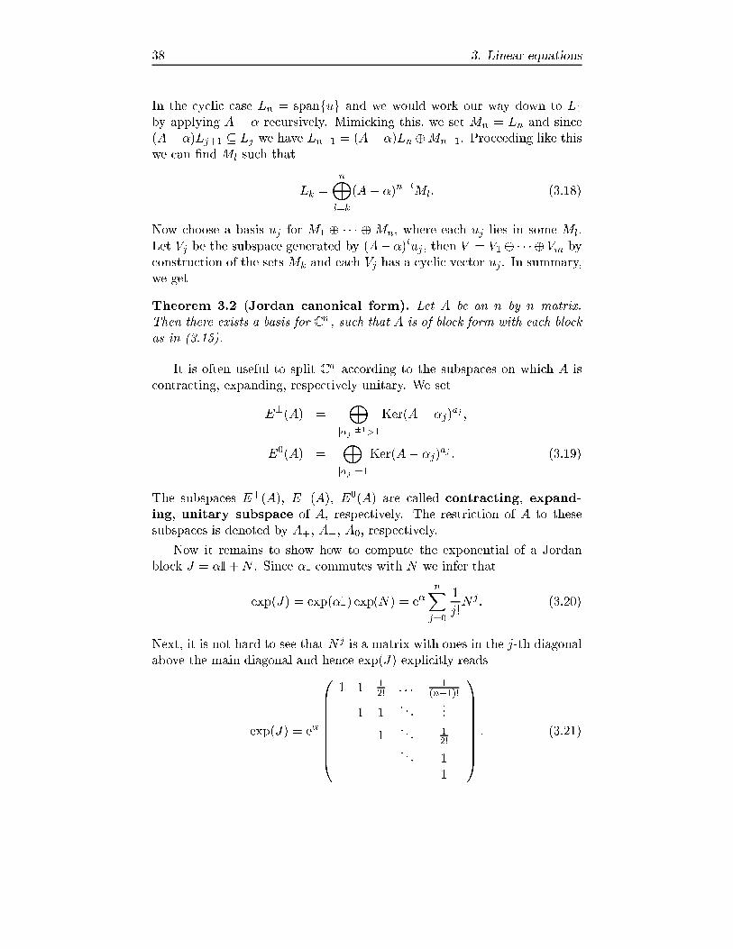
Theorem 3.2 (Jordan canonical form). Let A be an n by n matrix.
Then there exists a basis for C n , such that A is of block form with each block
as in (3.15).
It is often useful to split C n according to the subspaces on which A is
contracting, expanding, respectively unitary. We set
E�(A) =
Mj�j j�1>1
Ker(A� �j)aj ;
E0(A) =
Mj�j j=1
Ker(A� �j)aj : (3.19)
The subspaces E+(A), E�(A), E0(A) are called contracting, expand-
ing, unitary subspace of A, respectively. The restriction of A to these
subspaces is denoted by A+, A�, A0, respectively.
Now it remains to show how to compute the exponential of a Jordan
block J = �I+N . Since �I commutes with N we infer that
exp(J) = exp(�I) exp(N) = e�nXj=0
1
j!Nj: (3.20)
Next, it is not hard to see that N j is a matrix with ones in the j-th diagonal
above the main diagonal and hence exp(J) explicitly reads
exp(J) = e�
0BBBBBBB@
1 1 12! : : :
1(n�1)!
1 1. . .
...
1. . . 1
2!. . . 1
1
1CCCCCCCA: (3.21)

3.1. Preliminaries from linear algebra 39
Note that if A is in Jordan canonical form, then it is not hard to see
that
det(exp(A)) = exp(tr(A)): (3.22)
Since both the determinant and the trace are invariant under linear trans-
formations, the formula also holds in the general case.
In addition, to the matrix exponential we will also need its inverse. That
is, given a matrix A we want to �nd a matrix B such that
A = exp(B): (3.23)
Clearly, by (3.22) this can only work if det(A) 6= 0. Hence suppose that
det(A) 6= 0. It is no restriction to assume that A is in Jordan canonical
form and to consider the case of only one Jordan block, A = �I+N .
Motivated by the power series for the logarithm,
ln(1 + x) =
1Xj=1
(�1)jj
xj; jxj < 1; (3.24)
we set
B = ln(�)I�n�1Xj=1
(�1)jj�j
Nj
=
0BBBBBBB@
ln(�) 1�
�12�2
: : :(�1)n
(n�1)�n�1
ln(�) 1�
. . ....
ln(�). . . �1
2�2
. . . 1�
ln(�)
1CCCCCCCA: (3.25)
By construction we have exp(B) = A.
Let me emphasize, that both the eigenvalues and generalized eigenvec-
tors can be complex even if the matrix A has only real entries. Since in many
applications only real solutions are of interest, one likes to have a canon-
ical form involving only real matrices. This form is called real Jordan
canonical form and it can be obtained as follows.
Suppose the matrix A has only real entries. Let �i be its eigenvalues
and let uj be a basis in which A has Jordan canonical form. Look at the
complex conjugate of the equation
Auj = �iuj ; (3.26)
it is not hard to conclude the following for a given Jordan block J = �I+N :
If � is real, the corresponding generalized eigenvectors can assumed to
be real. Hence there is nothing to be done in this case.

40 3. Linear equations
If � is nonreal, there must be a corresponding block ~J = ��I+N and the
corresponding generalized eigenvectors can be assumed to be the complex
conjugates of our original ones. Therefore we can replace the pairs uj , u�j
in our basis by Re(uj) and Im(uj). In this new basis the block J � ~J is
replaced by 0BBBBBB@
R I
R I
R. . .
. . . I
R
1CCCCCCA; (3.27)
where
R =
�Re(�) Im(�)
�Im(�) Re(�)
�and I=
�1 0
0 1
�: (3.28)
Since the matrices �1 0
0 1
�and
�0 1
�1 0
�(3.29)
commute, the exponential is given by0BBBBBBB@
exp(R) exp(R) exp(R) 12! : : : exp(R) 1(n�1)!
exp(R) exp(R). . .
...
exp(R). . . exp(R) 1
2!. . . exp(R)
exp(R)
1CCCCCCCA; (3.30)
where
exp(R) = eRe(�)�
cos(Im(�)) � sin(Im(�))
sin(Im(�)) cos(Im(�))
�: (3.31)
Finally, let me remark that a matrix A(t) is called di�erentiable with re-
spect to t if all coeÆcients are. In this case we will denote by ddtA(t) � _A(t)
the matrix, whose coeÆcients are the derivatives of the coeÆcients of A(t).
The usual rules of calculus hold in this case as long as one takes noncom-
mutativity of matrices into account. For example we have the product rule
d
dtA(t)B(t) = _A(t)B(t) +A(t) _B(t) (3.32)
(Problem 3.1).
Problem 3.1 (Di�erential calculus for matrices.). Suppose A(t) and B(t)
are di�erentiable. Prove (3.32) (note that the order is important!). Suppose
det(A(t)) 6= 0, show
d
dtA(t)�1 = �A(t)�1 _A(t)A(t)�1

3.2. Linear �rst order systems 41
(Hint: AA�1 = I.)
Problem 3.2. (i) Compute exp(A) for
A =
�a+ d b
c a� d
�:
(ii) Is there a real matrix A such that
exp(A) =
� �� 0
0 ���; �; � > 0?
Problem 3.3. Denote by r(A) = maxjfj�j jg the spectral radius of A.
Show that for every " > 0 there is a norm k:k" such that
kAk" = supx: kxk"=1
kAxk" � r(A) + ":
(Hint: It suÆces to prove the claim for a Jordan block J = �I+N (why?).
Now choose a diagonal matrix Q = diag(1; "; : : : ; "n) and observe Q�1JQ =
�I+ "N .)
Problem 3.4. Suppose A(�) is Ck and has no unitary subspace. Then
the projectors P�(A(�)) onto the contracting, expanding subspace are Ck.
(Hint: Use the formulas
P+(A(�)) =
1
2�i
Zjzj=1
dz
z �A(�); P
�(A(�)) = I� P+(A(�)):)
3.2. Linear �rst order systems
We begin with the study of the homogeneous linear �rst order system
_x(t) = A(t)x(t); (3.33)
where A 2 C(I;Rn�Rn). Clearly, our basic existence and uniqueness result(Theorem 2.3) applies to this system. Moreover, if I = R, solutions exist
for all t 2 R by Theorem 2.11.
Now observe that linear combinations of solutions are again solutions.
Hence the set of all solutions is a vector space. This is often referred to
as principal of superposition. In particular, there is a linear mapping
x0 7! �(t; t0; x0) given by
�(t; t0; x0) = �(t; t0)x0; (3.34)
where
�(t; t0) = (�(t; t0; Æ1); : : : ; �(t; t0; Æn)): (3.35)
Here Æj;k = 1 if j = k and Æj;k = 0 if j 6= k. The matrix �(t; t0) is called
principal matrix solution and it solves the matrix valued initial value
problem_�(t; t0) = A(t)�(t; t0); �(t0; t0) = I: (3.36)

42 3. Linear equations
Furthermore, it satis�es
�(t; t1)�(t1; t0) = �(t; t0) (3.37)
since both sides solve _� = A(t)� and coincide for t = t1. In particular,
�(t; t0) is an isomorphism with inverse �(t; t0)�1 = �(t0; t).
Let us summarize the most important �ndings in the following theorem.
Theorem 3.3. The solutions of the system (3.33) form an n dimensional
vector space. Moreover, there exists a matrix-valued solution �(t; t0) such
that the solution of the IVP x(t0) = x0 is given by �(t; t0)x0.
More generally, taking n solutions �1; : : : ; �n we obtain a matrix solu-
tion U(t) = (�1(t); : : : ; �n(t)). The determinant of U(t) is called Wronski
determinant
W (t) = det(�1(t); : : : ; �n(t)): (3.38)
If detU(t) 6= 0, the matrix solution U(t) is called a fundamental matrix
solution. Moreover, if U(t) is a matrix solution, so is U(t)C, where C
is a constant matrix. Hence, given two fundamental matrix solutions U(t)
and V (t) we always have V (t) = U(t)U(t0)�1V (t0) since a matrix solution
is uniquely determined by an initial condition. In particular, the principal
matrix solution can be obtained from any fundamental matrix solution via
�(t; t0) = U(t)U(t0)�1.
The following lemma shows that it suÆces to check detU(t) 6= 0 for one
t 2 R.
Lemma 3.4 (Liouville). The Wronski determinant of n solutions satis�es
W (t) =W (t0) exp
�Z t
t0
tr(A(s)) ds
�: (3.39)
This is known as Liouville's formula.
Proof. Using U(t+ ") = �(t+ "; t)U(t) and
�(t+ "; t) = I+A(t)"+ o(") (3.40)
we obtain
W (t+ ") = det(I+A(t)"+ o("))W (t) = (1 + tr(A(t))"+ o("))W (t) (3.41)
(this is easily seen by induction on n) implying
d
dtW (t) = tr(A(t))W (t): (3.42)
This equation is separable and the solution is given by (3.39). �

3.2. Linear �rst order systems 43
Now let us turn to the inhomogeneous system
_x = A(t)x+ g(t); x(t0) = x0; (3.43)
where A 2 C(I;Rn � Rn) and g 2 C(I;Rn). Since the di�erence of two
solutions of the inhomogeneous system (3.43) satis�es the corresponding
homogeneous system (3.33), it suÆces to �nd one particular solution. This
can be done using the following ansatz
x(t) = �(t; t0)c(t); c(t0) = x0; (3.44)
which is known as variation of constants. Di�erentiating this ansatz we
see
_x(t) = A(t)x(t) + �(t; t0) _c(t) (3.45)
and comparison with (3.43) yields
_c(t) = �(t0; t)g(t); (3.46)
Integrating this equation shows
c(t) = x0 +
Z t
t0
�(t0; s)g(s)ds (3.47)
and we obtain
Theorem 3.5. The solution of the inhomogeneous system corresponding to
the initial condition x(t0) = x0 is given by
x(t) = �(t; t0)x0 +
Z t
t0
�(t; s)g(s)ds; (3.48)
where �(t; t0) is the principal matrix solution of the corresponding homoge-
neous system.
Problem 3.5. Solve the following equations.
(i) _x = 3x.
(ii) _x = t x, 2 R.
(iii) _x = x+ sin(t).
Problem 3.6. Consider the equation �x = q(t)x+ g(t).
(i) Show that the Wronski determinant
W (u; v) = u(t)v0(t)� u0(t)v(t)
of two solutions u, v of the homogeneous equation is independent of t.
(ii) Show that the fundamental matrix of the associated system is given
by
�(t; s) =1
W (u; v)
�u(t)v0(s)� v(t)u0(s) v(t)u(s) � v(s)u(t)
v0(s)u0(t)� v
0(t)u0(s) u(s)v0(t)� v(s)u0(t)
�

44 3. Linear equations
and use the variation of constants formula to show that
x(t) =u(t)
W (u; v)
Z t
v(s)g(s)ds � v(t)
W (u; v)
Z t
u(s)g(s)ds
is a solutions of the inhomogeneous equation.
(iii) Given one solution u(t) of the homogeneous equation, make a vari-
ation of constants ansatz v(t) = c(t)u(t) and show that a second solution is
given by
v(t) = u(t)
Z t 1
u(s)2ds:
(iv) Show that if u is a solution of the homogeneous equation, then � =
u0=u satis�es the Riccati equation
�0 + �
2 = q(t):
Problem 3.7 (Reduction of order (d'Alembert)). Look at the n-th order
equation
x(n) + qn�1(t)x
(n�1) + � � �+ q1(t) _x+ q0(t)x = 0:
Show that if one solutions x1(t) is known, the variation of constants ansatz
x(t) = c(t)x1(t) gives a (n� 1)-th order equation for _c. Hence the order can
be reduced by one.
Problem 3.8 (Quantum Mechanics). A quantum mechanical system which
can only attain �nitely many states is described by a complex valued vector
(t) 2 Cn . The square of the absolute values of the components j j j2 are
interpreted as the probability of �nding the system in the j-th state at time
t. Since there are only n possible states, these probabilities must add up to
one, that is, (t) must be normalized, j j = 1. The time evolution of the
system is governed by the Schr�odinger equation
i _ (t) = H(t) (t); (t0) = 0;
where H(t), is a self-adjoint matrix, that is, H(t)� = H(t). Here H(t) is
called the Hamiltonian and describes the interaction. Show that the solution
is given by
(t) = U(t; t0) 0;
where U(t; t0) is unitary, that is, U(t; t0)�1 = U(t; t0)
� (Hint: Problem 3.1).
Conclude that (t) remains normalized for all t if 0 is.
Each observable (quantity you can measure) corresponds to a self-adjoint
matrix, say L0. The expectation value for a measurement of L0 if the system
is in the state (t) is given by
h (t); L0 (t)i;

3.3. Periodic linear systems 45
where h'; i = '� is the scalar product in C
n . Show that
d
dth (t); L0 (t)i = ih (t); [H(t); L0] (t)i
and conclude that the solution of the Heisenberg equation
_L(t) = i[H(t); L(t)] + _H(t); L(t0) = L0;
where [H;L] = HL� LH is the commutator, is given by
L(t) = U(t0; t)L0U(t; t0):
3.3. Periodic linear systems
In this section we want to consider (3.33) in the special case where A(t) is
periodic,
A(t+ T ) = A(t); T > 0: (3.49)
This periodicity condition implies that x(t+T ) is again a solution if x(t) is.
Hence it suggests itself to investigate what happens if we move on by one
period, that is, to look at the monodromy matrix
M(t0) = �(t0 + T; t0): (3.50)
A �rst naive guess would be that all initial conditions return to their
starting values after one period (i.e., M(t0) = I) and hence all solutions are
periodic. However, this is too much to hope for since it already fails in one
dimension with A(t) a constant.
On the other hand, since it does not matter whether we start our period
at t0, at t0+ T , or even t0+ `T , ` 2 Z, we infer that M(t0) is periodic, that
is, M(t0 + T ) = M(t0). Moreover, we even have �(t0 + `T; t0) = M(t0)`.
Thus �(t; t0) exhibits an exponential behavior if we move on by one period
in each step. If we factor out this exponential term, the remainder should
be periodic.
For this purpose we rewrite M(t0) a little bit. By Liouville's formula
the determinant of the monodromy matrix
det(M(t0)) = exp
�Z t0+T
t0
tr(A(s))ds
�= exp
�Z T
0
tr(A(s))ds
�(3.51)
is independent of t0 and positive. Hence there is a matrix Q(t0) (which is
not unique) such that
M(t0) = exp(TQ(t0)); Q(t0 + T ) = Q(t0): (3.52)
Writing
�(t; t0) = P (t; t0) exp((t� t0)Q(t0)) (3.53)

46 3. Linear equations
a straightforward computation shows that
P (t+ T; t0) = �(t+ T; t0)M(t0)�1e�(t�t0)Q(t0)
= �(t+ T; t0 + T )e�(t�t0)Q(t0)
= �(t; t0)e�(t�t0)Q(t0) = P (t; t0) (3.54)
as anticipated. In summary we have proven Floquet's theorem.
Theorem 3.6 (Floquet). Suppose A(t) is periodic, then the principal matrix
solution of the corresponding linear system has the form
�(t; t0) = P (t; t0) exp((t� t0)Q(t0)); (3.55)
where P (:; t0) has the same period as A(:) and P (t0; t0) = I.
Note that any fundamental matrix solution can be written in this form
(Problem 3.9).
Hence to understand the behavior of solutions one needs to understand
the Jordan canonical form of the monodromy matrix. Moreover, we can
choose any t0 since M(t1) and M(t0) are similar matrices by virtue of
M(t1) = �(t1; t0)M(t0)�(t1; t0)�1: (3.56)
Thus the eigenvalues and the Jordan structure is independent of t0 (hence
the same also follows for Q(t0)).
Before I show how this result is used in a concrete example, let me
note another consequence of Theorem 3.6. The proof is left as an exercise
(Problem 3.10).
Corollary 3.7. The transformation y(t) = P (t; t0)�1x(t) renders the sys-
tem into one with constant coeÆcients,
_y(t) = Q(t0)y(t): (3.57)
Note also that we have P (t; t0)�1 = exp((t� t0)Q(t0))P (t0; t) exp(�(t�
t0)Q(t0)) by virtue of �(t; t0)�1 = �(t0; t).
One of the most prominent examples is Hill's equation
�x+ q(t)x = 0; q(t+ T ) = q(t): (3.58)
In this case
�(t; t0) =
�c(t; t0) s(t; t0)
_c(t; t0) _s(t; t0)
�; (3.59)
where c(t; t0) is the solution corresponding to the initial condition c(t0; t0) =
1, _c(t0; t0) = 0 and similarly for s(t; t0). Liouville's formula shows
det�(t; t0) = 1 (3.60)

3.3. Periodic linear systems 47
and hence the characteristic equation for M(t) is given by
�2 � 2��+ 1 = 0; (3.61)
where
� =tr(M(t))
2=c(t+ T; t) + _s(t+ T; t)
2: (3.62)
If �2> 1 we have two di�erent real eigenvalues
�� = ��p�2 � 1 = � e�T ; �
2 = 1; > 0; (3.63)
with corresponding eigenvectors
u�(t0) =
1
���c(t0+T;t0)s(t0+T;t0)
!=
1
_s(t0+T;t0)��� _c(t0+T;t0)
!: (3.64)
Considering
�(t; t0)u�(t0) = P (t; t0) exp((t� t0)Q(t0))u�(t0)
= � e� (t�t0)P (t; t0)u�(t0); (3.65)
we see that there are two solutions of the form
e� tp�(t); > 0; p�(t+ T ) = � p�(t); (3.66)
where � = sgn(�). Similarly, if �2< 1 we have two di�erent purely complex
eigenvalues and hence two solutions
e�i tp�(t); > 0; p�(t+ T ) = p�(t): (3.67)
If �2 = 1 we have either two solutions
p�(t); p�(t+ T ) = � p�(t); (3.68)
or two solutions
p+(t); p�(t) + tp+(t); p�(t+ T ) = � p�(t): (3.69)
A periodic equation is called stable if all solutions are bounded. Thus
we have shown
Theorem 3.8. Hills equation is stable if j�j < 1 and unstable if j�j > 1.
This result is of high practical importance in applications. For example,
the potential of a charged particle moving in the electric �eld of a quadrupole
is given by
U(x) = eV
a2(x2 � y
2):

48 3. Linear equations
If we set for the voltage V = V0+V1 cos(t), one gets the following equations
of motion (neglecting the induced magnetic �led)
�x = � 2e
ma2(V0 + V1 cos(t))x;
�y = +2e
ma2(V0 + V1 cos(t))y;
�z = 0: (3.70)
The equation for the x and y coordinates is the Mathieu equation
�x = !2(1 + " cos(t))x: (3.71)
A numerically computed stability diagram for 0 � ! � 3 and �1:5 � " � 1:5
is depicted below.
The shaded regions are the ones where �(!; ")2 > 1, that is, where the
equation is unstable. Observe that these unstable regions emerge from the
points 2! 2 N0 where �(!; 0) = cos(2�!) = �1.Varying the voltages V0 and V1 one can achieve that the equation is only
stable (in the x or y direction) if the mass of the particle lies in a certain
region. This can be used to �lter charged particles according to their mass.
Problem 3.9. Show that any fundamental matrix solution U(t) of a periodic
linear system can be written as U(t) = V (t) exp(tR), where V (t) is periodic
and R is similar to Q(t0).
Problem 3.10. Prove Corollary 3.7.
Problem 3.11. Consider the inhomogeneous equation
_x(t) = A(t)x(t) + g(t);
where both A(t) and g(t) are periodic of period T . Show that this equation
has a periodic solution of period T if 1 is not an eigenvalue of the monodromy
matrix M(t0). (Hint: Note that x(t) is periodic if and only if x(T ) = x(0)
and use the variation of constants formula (3.48).)
Problem 3.12 (Re ection symmetry). Suppose q is periodic q(t+T ) = q(t)
and symmetric q(�t) = q(t). Prove

3.4. Linear autonomous �rst order systems 49
(i) c(�t) = c(t) and s(�t) = �s(t),(ii) c(t�T ) = c(T )c(t)� _c(T )s(t) and s(t�T ) = �s(T )c(t)+ _s(T )s(t),
(iii) c(T ) = _s(T ),
where c(t; 0) = c(t), s(t; 0) = s(t).
Problem 3.13 (Resonance). Solve the equation
�x+ !2x = cos(�t); !; � > 0:
Discuss the behavior of solutions as t!1.
Problem 3.14. A simple quantum mechanical model for an electron in a
crystal leads to the investigation of
�y00 + q(x)y = �y; where q(x+ 1) = q(x):
The parameter � 2 R corresponds to the energy of the electron. Only energies
for which the equation is stable are allowed and hence the set � = f� 2Rjj�(�)j � 1g is called the spectrum of the crystal. Since �(�) is continuous
with respect to �, the spectrum consists of bands with gaps in between.
Consider the explicit case
q(x) = q0; 0 � x <1
2; q(x) = 0;
1
2� x < 1:
Show that there are no spectral bands below a certain value of �. Show that
there is an in�nite number of gaps if q0 6= 0. How many gaps are there for
q0 = 0? (Hint: Set �� q0 ! (a� ")2 and �! (a+ ")2 in the expression for
�(�). If q0 ! 0, where would you expect gaps to be? Choose these values
for a and look at the case a!1.)
3.4. Linear autonomous �rst order systems
We now turn to the autonomous linear �rst order system
_x = Ax: (3.72)
In this case the Picard iteration can be computed explicitly, producing
xn(t) =
nXj=0
tj
j!Ajx0: (3.73)
The limit as n!1 is given by
x(t) = limn!1
xn(t) = exp(tA)x0: (3.74)
Hence in order to understand the dynamics of the system (3.72), we need
to understand the properties of the function
�(t; t0) = �(t� t0) = exp((t� t0)A): (3.75)

50 3. Linear equations
This is best done by using a linear change of coordinates
y = Ux (3.76)
which transforms A into a simpler form UAU�1. The form most suitable
for computing the exponential is the Jordan canonical form, discussed in
Section 3.1. In fact, if A is in Jordan canonical form, it is not hard to
compute exp(tA). It even suÆces to consider the case of one Jordan block,
where it is not hard to see that
exp(tJ) = e�t
0BBBBBBB@
1 tt2
2!: : :
tn�1
(n�1)!
1 t. . .
...
1. . . t2
2!. . . t
1
1CCCCCCCA: (3.77)
On the other hand, the procedure of �nding the Jordan canonical form is
quite cumbersome and hence we will use Mathematica to do the calculations
for us. For example, let
In[1]:= A =
0@ �11 �35 �24
�1 �1 �28 22 17
1A ;
Then the command
In[2]:= fU; Jg = JordanDecomposition[A];
gives us the transformation matrix U plus the Jordan canonical form J =
U�1AU .
In[3]:= J == MatrixForm
Out[3]//MatrixForm=0@ 1 0 0
0 2 1
0 0 2
1A
If you don't trust me (or Mathematica), you can also check it:
In[4]:= A == U:J:Inverse[U]
Out[4]= True
Furthermore, Mathematica can even compute the exponential for us
In[5]:= MatrixExp[tJ] == MatrixForm
Out[5]//MatrixForm=
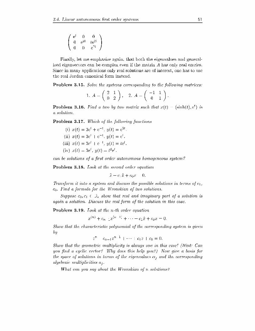
3.4. Linear autonomous �rst order systems 51
0@ et 0 0
0 e2t te2t
0 0 e2t
1A
Finally, let me emphasize again, that both the eigenvalues and general-
ized eigenvectors can be complex even if the matrix A has only real entries.
Since in many applications only real solutions are of interest, one has to use
the real Jordan canonical form instead.
Problem 3.15. Solve the systems corresponding to the following matrices:
1: A =
�2 1
0 2
�; 2: A =
� �1 1
0 1
�:
Problem 3.16. Find a two by two matrix such that x(t) = (sinh(t); et) is
a solution.
Problem 3.17. Which of the following functions
(i) x(t) = 3et + e�t, y(t) = e2t.
(ii) x(t) = 3et + e�t, y(t) = et.
(iii) x(t) = 3et + e�t, y(t) = tet.
(iv) x(t) = 3et, y(t) = t2et.
can be solutions of a �rst order autonomous homogeneous system?
Problem 3.18. Look at the second order equation
�x+ c1 _x+ c0x = 0:
Transform it into a system and discuss the possible solutions in terms of c1,
c0. Find a formula for the Wronskian of two solutions.
Suppose c0; c1 2 R, show that real and imaginary part of a solution is
again a solution. Discuss the real form of the solution in this case.
Problem 3.19. Look at the n-th order equation
x(n) + cn�1x
(n�1) + � � � + c1 _x+ c0x = 0:
Show that the characteristic polynomial of the corresponding system is given
by
zn + cn�1z
n�1 + � � �+ c1z + c0 = 0:
Show that the geometric multiplicity is always one in this case! (Hint: Can
you �nd a cyclic vector? Why does this help you?) Now give a basis for
the space of solutions in terms of the eigenvalues �j and the corresponding
algebraic multiplicities aj.
What can you say about the Wronskian of n solutions?

52 3. Linear equations
Problem 3.20. Consider the n-th order equation
x(n) + cn�1x
(n�1) + � � �+ c1 _x+ c0x = g(t)
and use the variation of constants formula to show that a solution of the
inhomogeneous equation is given by
x(t) =
Z t
0
u(t� s)g(s)ds;
where u(t) is the solution of the homogeneous equation corresponding to the
initial condition u(0) = _u(0) = � � � = u(n�1)(0) = 0 and u(n)(0) = 1.
Problem 3.21 (Euler equation). Show that the equation
�x+c1
t_x+
c0
t2x = 0; t > 0;
can be solved by introducing the new dependent variable � = ln(t). Discuss
the possible solutions for c0; c1 2 R.
Problem 3.22 (Laplace transform). Consider the Laplace transform
L(x)(s) =Z 1
0
e�stx(t)dt:
show that the initial value problem
_x = Ax+ f(t); x(0) = x0
is transformed into a linear system of equations by the Laplace transform.

Chapter 4
Di�erential equations
in the complex domain
4.1. The basic existence and uniqueness result
Until now we have only imposed rather weak requirements on the smoothness
of our di�erential equations. However, on the other hand, most examples
encountered were in fact (real) analytic. Up to this point we did not use
this additional information, but in the present chapter I want to show how
to gain a better understanding for these problems by taking the detour over
the complex plane. Readers only interested in dynamical systems can skip
this and the next chapter and go directly to Chapter 6.
In this chapter we want to look at di�erential equations in a complex
domain � Cn+1 . We suppose that
f : ! C ; (z; w) 7! f(z; w); (4.1)
is analytic in and consider the equation
w0 = f(z; w); w(z0) = w0: (4.2)
Here the prime denotes complex di�erentiation and hence the equation only
makes sense if w is analytic as well. Clearly, the �rst question to ask is
whether solutions exist at all. Fortunately, this can be answered using the
same tools as in the real case. It suÆces to only point out the di�erences.
The �rst step is to rewrite (4.2) as
w(z) = w0 +
Z z
z0
f(�; w)d�: (4.3)
53
54 4. Di�erential equations in the complex domain
But note that we now have to be more careful since the integral is along a
path in the complex plane and independence of the path is not clear. On
the other hand, we will only consider values of z in a small disc around
z0. Since a disc is simply connected, path independence follows from the
Cauchy integral theorem. Next, we need a suitable Banach space. As in the
real case we can use the sup norm
supjz�z0j<"
jw(z)j (4.4)
since the uniform limit of a sequence of analytic functions is again analytic.
Now we can proceed as in the real case to obtain
Theorem 4.1. Suppose f : ! C is analytic. Then the initial value prob-
lem (4.2) has a unique solution de�ned in a suÆciently small disc around
z0.
Next, let us look at maximally de�ned solutions. Unfortunately, this
topic is more tricky than in the real case. In fact, let w1(z) and w2(z) be
two solutions de�ned on the domains U1 and U2 respectively. Then they
coincide in a neighborhood of z0 by our local uniqueness result. Hence they
also coincide on the connected component of U1\U2 containing z0. But thisis all we can say in general as the example
w0 =
1
z; w(1) = 0; z 2 C nf0g; (4.5)
shows. Indeed, the solution is given by w(z) = ln(z) and di�erent choices of
the branch cut will give di�erent solutions.
These problems do not arise if is simply connected.
Theorem 4.2. Suppose � C is simply connected and z0 2 . Then the
initial value problem (4.2) has a unique solution de�ned on all of .
Proof. Pick z 2 and let : [0; 1] ! be a path from z0 to z. Around
each point (t0) we have a solution of the di�erential equation w0 = f(z; w)
and by local uniqueness we can choose the solutions in such a way that they
coincide for t close to t0. So we can de�ne the value of w(z) by analytic
continuation along the path . Since is simply connected, this value is
uniquely de�ned by the monodromy theorem. �
Finally, let us investigate the simple example
w0 =
1
z; w(1) = 0; z 2 C nf0g; (4.6)
to show you how analyticity can be used in the investigation of a simple
di�erential equation,
w0 + w
2 = z; w(0) = w0: (4.7)
4.2. Linear equations 55
This is a Riccati equation and we already know that it cannot be solved
unless we �nd a particular solution. However, after you have tried for some
time you will agree that it seems not possible to �nd one and hence we need
to try something di�erent. Since we know that the solution is analytic near
0 we can at least write
w(z) =
1Xj=0
wjzj (4.8)
and plugging this into our equation yields
1Xj=0
jwjzj�1 +
0@ 1Xj=0
wjzj
1A
2
= z: (4.9)
Expanding the product and aligning powers of z gives
1Xj=0
(j + 1)wj+1 +
jXk=0
wjwk�j
!zj = z: (4.10)
Comparing powers of z we obtain
w1 = �w20; w2 = w
30 +
1
2; wj+1 =
�1j + 1
jXk=0
wjwk�j: (4.11)
Hence we have at least found a recursive formula for computing the coeÆ-
cients of the power series of the solution. However, I should point out that
this will no longer work if the function f involves w in a too complicated
way. Hence we will only investigate the case of linear equations further. In
fact, this will eventually allow us to solve the above equation using special
functions (Problem 4.7). However, we will on the other hand allow for poles
in the coeÆcients, which is often needed in applications.
The following two sections are quite technical and can be skipped if you
are not interested in the details of the proof of the generalized power series
method alluded to above.
Problem 4.1. Try to �nd a solution of the initial value problem
w00 = (z2 � 1)w; w(0) = 0;
by using the power series method from above.
4.2. Linear equations
For the rest of this chapter we will restrict our attention to linear equations
which are the most important ones in applications. That is, we will look at
the equation
w0 = A(z)w; w(z0) = w0; z; z0 2 � C ; (4.12)

56 4. Di�erential equations in the complex domain
where A(z) is a matrix whose coeÆcients are analytic in . Note that, as
in the real case, the superposition principle holds. Hence, we can �nd a
principal matrix solution �(z; z0) such that the solution of (4.12) is given
by
w(z) = �(z; z0)w0 (4.13)
at least for z in a neighborhood of z0. It is also not hard to see that Liouville's
formula extends to the complex case. Moreover, if is simply connected,
we can extend solutions to the entire domain .
In summary, we now know that the solution is nice whenever the matrix
A(z) is analytic. However, in most applications the coeÆcients will have
singularities and one of the main questions is the behavior of the solutions
near such a singularity. This will be our next topic. But �rst let us look at
a prototypical example.
The system
w0 =
1
zAw; z 2 C nf0g; (4.14)
is called Euler system. Obviously it has a �rst order pole at z = 0 and
since C nf0g is not simply connected, solutions might not be de�ned for all
z 2 C nf0g. Hence we introduce a branch cut along the negative real axis
and consider the simply connected domain = C n(�1; 0]. To solve (4.14)
we will use the transformation
� = ln(z) = ln jzj+ i arg(z); �� < arg(z) < �; (4.15)
which maps to the strip ~ = fz 2 C j � � < Im(z) < �g. The equation in
the new coordinates reads
!0 = A!; !(�) = w(e�): (4.16)
Hence a fundamental system is given by
W (z) = zA = exp(ln(z)A); (4.17)
where the last expression is to be understood as the de�nition of zA. As
usual, zA can be easily computed if A is in Jordan canonical form. In
particular, for a Jordan block J we obtain
zJ = z
�
0BBBBBBB@
1 ln(z)ln(z)2
2! : : :ln(z)n�1
(n�1)!
1 ln(z). . .
...
1. . . ln(z)2
2!. . . ln(z)
1
1CCCCCCCA: (4.18)

4.2. Linear equations 57
Therefore the solution consists of terms of the form z� ln(z)k, where � is an
eigenvalue of A and k is a nonnegative integer. Note that the logarithmic
terms are only present if A is not diagonalizable.
This behavior is in fact typical near any isolated singularity as the fol-
lowing result shows.
Theorem 4.3. Suppose A(z) is analytic in = fz 2 C j0 < jz � z0j < "g.Then a fundamental system of w0 = A(z)w is of the form
W (z) = U(z)(z � z0)M; (4.19)
where U(z) is analytic in .
Proof. Again we use our change of coordinates � = ln(z) to obtain
!0 = e�A(e�)!; Re(�) < ln("): (4.20)
But this system is periodic with period 2�i and hence the result follows as
in the proof of Floquet's theorem (Theorem 3.6). �
Observe that any other fundamental system ~W (z) can be written as
~W (z) =W (z)C = U(z)C (z � z0)C�1MC
; det(C) 6= 0; (4.21)
and hence has a representation ~W (z) = ~U(z)(z � z0) ~M , where ~M is linearly
equivalent to M .
Please note that this theorem does not say that all the bad terms are
sitting in (z � z0)B . In fact, U(z) might have an essential singularity at z0.
However, if this is not the case, the singularity is called regular and we can
easily absorb the pole of U(z) in the (z � z0)B term by using
W (z) = U(z)(z � z0)n (z � z0)
B�nI: (4.22)
But when can this be done? We expect this to be possible if the singularity
of A(z) is not too bad. However, the equation w0 = 1z2w has the solution
w(z) = exp(�1z ), which has an essential singularity at 0. Hence our only
hope left are �rst order poles. We will say that z0 is a simple singularity
of our system if A(z) has a pole of (at most) �rst order at z0.
Theorem 4.4. Suppose A(z) is analytic in = fz 2 C j0 < jz�z0j < "g andhas a simple singularity at z0. Then U(z) in (4.19) can be chosen analytic
in fz 2 C j jz � z0j < "g.
Proof. It is no restriction to consider z0 = 0 and it suÆces to show that
U(z) can have at most a pole. Let w(z) be any solution. Moreover, for

58 4. Di�erential equations in the complex domain
given r0 > 0 we can �nd a number n such that kA(z)k � njzj . Using polar
coordinates z = rei' we have
jw(rei')j � jw(r0ei')j+Z r0
r
n
sjw(sei')jds (4.23)
for 0 < r � r0. Applying Gronwall and taking the maximum over all ' we
obtain
jw(z)j � sup�:j�j=r0
jw(�)j���r0z
���n ; (4.24)
which is the desired estimate. �
The converse of this result is in general not true, however, note that
A(z) = U0(z)U(z)�1 +
1
z � z0U(z)MU(z)�1 (4.25)
shows that A(z) cannot have an essential singularity if U(z) has none.
Lemma 4.5. If z0 is a regular singularity, then A(z) has at most a pole at
z0.
In the case to second order equations
u00 + p(z)u0 + q(z)u = 0 (4.26)
the situation is a bit simpler and the converse can be established. Trans-
forming (4.26) to a system as usual shows that z0 is a simple singularity if
both p(z) and q(z) have at most a �rst order pole. However, we can do even
better. Introducing w(z) = (u(z); z u0(z)) we obtain
w0 = A(z)w; A(z) =
�0 1
z�zq(z) 1
z � p(z)
�(4.27)
and z0 = 0 is a simple singularity if p(z) and zq(z) have at most �rst order
poles. This is even optimal.
Theorem 4.6 (Fuchs). The system (4.27) has a regular singularity at z0 if
and only if p(z) and zq(z) have at most �rst order poles.
Proof. If (4.27) has a regular singularity, there is a solution of the form
u(z) = z�h(z), where h(0) = 1 and h(z) is analytic near 0. Let v(z) be a
linearly independent solution and consider c(z) = v(z)=u(z). Then, since
c(z) has no essential singularity,
p(z) = �c00(z)
c0(z)� 2
u0(z)
u(z)(4.28)
has a �rst order pole. Moreover,
q(z) = �u00(z)
u(z)� p(z)
u0(z)
u(z)(4.29)

4.3. The Frobenius method 59
has at most a second order pole. �
I remark that using induction on the order of the di�erential equation,
one can show the analogous result for n-th order equations.
Problem 4.2. Let z0 be a simple singularity and let W (z) be a fundamental
system as in (4.19). Show that
det(W (z)) = (z � z0)tr(A0)d(z); d(z0) 6= 0;
where d(z) is analytic near z0 and A0 = limz!z0(z � z0)A(z). Moreover,
conclude that tr(A0�M) 2 Z. (Hint: Use Liouville's formula for the deter-
minant.)
4.3. The Frobenius method
In this section we pursue our investigation of simple singularities. Without
loss of generality we will set z0 = 0. Since we know how a fundamental
system looks like from Theorem 4.4, we can make the ansatz
W (z) = U(z)zM ; U(z) =
1Xj=0
Ujzj; U0 6= 0: (4.30)
Using
A(z) =1
z
1Xj=0
Ajzj (4.31)
and plugging everything into our di�erential equation yields the recurrence
relation
Uj (j +M) =
jXk=0
AkUj�k (4.32)
for the coeÆcients Uj. However, since we don't know M this does not help
us much. By (4.17) you could suspect that we just haveM = A0 and U0 = I.
Indeed, if we assume det(U0) 6= 0, we obtain U0M = A0U0 for j = 0 and
hence W (z)U�10 = U(z)U�1
0 zA0 is of the anticipated form. Unfortunately,
we don't know that det(U0) 6= 0 and, even worse, this is wrong in general
(examples will follow).
So let us be less ambitious and look for a single solution �rst. If � is an
eigenvalue with corresponding eigenvector u0 of M , then
w0(z) =W (z)u0 = z�U(z)u0 (4.33)
is a solution of the form
w0(z) = z�u0(z); u0(z) =
1Xj=0
u0;jzj; u0;0 6= 0; � = �+m; (4.34)

60 4. Di�erential equations in the complex domain
m 2 N0 . Inserting this ansatz into our di�erential equation we obtain
(A0 � �� j)u0;j +
jXk=1
Aku0;j�k = 0: (4.35)
In particular, for j = 0,
(A0 � �)u0;0 = 0; (4.36)
we see that � must be an eigenvalue of A0!
Now what about the case where � corresponds to a nontrivial Jordan
block of size n > 1? Then, by (4.18), we have a corresponding set of gener-
alized eigenvectors ul, 1 � l � n, such that
wl(z) =W (z)ul = z�
�ul(z) + ln(z)ul�1(z) + � � �+ ln(z)l
l!u0(z)
�; (4.37)
1 � l � n, are n solutions. Here
ul(z) = z���
U(z)ul =
1Xj=ml
ul;jzj; ul;ml
6= 0; 1 � l � n; (4.38)
and we set ul;j = 0 for j < ml and u�1;j = 0 for notational convenience later
on.
Again, inserting this ansatz into our di�erential equation, we obtain
(A0 � �� j)ul;j +
jXk=1
Akul;j�k = ul�1;j: (4.39)
Considering j < ml we see ul�1;j = 0 for j < ml and thus ml�1 � ml. In
particular, �ml 2 N0 since m0 = 0. Furthermore, for j = ml we get
(A0 � ��ml)ul;ml= ul�1;ml
: (4.40)
Hence there are two cases, ml = ml�1 and (A0 � ��ml)ul;ml= ul�1;ml�1
,
that is, �+ml�1 corresponds to a nontrivial Jordan block of A0. Or ml >
ml�1 and (� +ml � A0)ul;ml= 0, that is, � +ml is another eigenvalue of
A0.
So we have found a quite complete picture of the possible forms of solu-
tions of our di�erential equation in the neighborhood of the singular point
z = 0 and we can now try to go the opposite way. Given a solution of the
system of linear equations (4.39), where � is an eigenvalue of A0 we get a
solution of our di�erential equation via (4.37) provided we can show that
the series converges.
But before turning to the problem of convergence, let us re ect about
how to solve the system (4.39). If the numbers � + j are not eigenvalues
of A0 for j > 0, we can multiply (4.39) by (� +ml + j � A0)�1 and ul;j is
uniquely determined by ul;j�1. Whereas this might not always be true, it

4.3. The Frobenius method 61
is at least true for j > j0 with j0 suÆciently large. Hence we are left with
a �nite system for the coeÆcients ul;j, 0 � l � n, 0 � j � j0, which we
can solve �rst. All remaining coeÆcients are then determined uniquely in a
recursive manner.
Theorem 4.7. Suppose ul;j solves (4.39), then ul(z) de�ned via the power
series (4.38) has the same radius of convergence as the power series for
zA(z) around z = 0. Moreover, wl(z) de�ned via (4.37) is a solution of
w0 = A(z)w.
Proof. Suppose Æ is smaller than the radius of convergence of the power
series for zA(z) around z = 0. We equip the space of expansion coeÆcients
with the norm (Problem 4.3)
kujk =1Xj=0
jujj Æj : (4.41)
The idea is now to cut o� the �rst j0 terms which cause trouble and view
the rest as a �xed point equation in the above Banach space. Let
Kuj =
(0 j � j01
+j
Pjk=0Akuj�k j > j0
; (4.42)
then
kKujk � 1
j0 � jRe( )j1Xj=0
jXk=0
jAj�kj jukjÆj =kAjk
j0 � jRe( )jkujk: (4.43)
Hence for j0 suÆciently large, the equation uj = vj + Kuj has a unique
solution by the contraction principle for any �xed vj. Now let ul;j be a
solution of (4.39) and choose = �+ml and vj = ul;j for j � j0 respectively
vj = � 1�+ml+j
ul�1;j for j > j0. Then the solution of our �xed point problem
coincides with our solution ul;j of (4.39) by construction. �
This procedure for �nding the general solution near a simple singularity
is known as Frobenius method. The eigenvalues of A0 are also called
characteristic exponents. Observe that our requirement of the singular-
ity to be simple is indeed crucial, since it ensures that the algebraic system
of equations for the coeÆcients can be solved recursively.
Finally, let me remark, that we can also try to apply this procedure
to get a power series around in�nity. To do this, one makes the change of
coordinates � = 1z , then our system transforms to
!0 = � 1
�2A(
1
�)!; w(z) = !(
1
z): (4.44)

62 4. Di�erential equations in the complex domain
In particular, 1 is a simple singularity if and only if A(z) has (at least) a
�rst order zero at 1, that is,
A(1
�) = �
1Xj=0
Aj�j: (4.45)
A system is called a Fuchs system if it has only �nitely many singularities
all of which, including in�nity, are simple. It then follows from Liouville's
theorem (every bounded analytic function is constant) that A(z) must be
rational.
Lemma 4.8. Every Fuchs system is of the form
A(z) =
kXj=1
Aj
z � zj: (4.46)
Problem 4.3. Show that the set of all complex-valued sequences fujgj2N0together with
kujk =1Xj=0
juj jwj ;
where the weights wj > 0 are �xed, is a Banach space.
4.4. Second order equations
In this section we want to apply our theory to second order equations
u00 + p(z)u0 + q(z)u = 0 (4.47)
We will assume that the singular point is z0 = 0 for notational convenience
and that the coeÆcients are of the form
p(z) =1
z
1Xj=0
pjzj; q(z) =
1
z2
1Xj=0
qjzj; (4.48)
such that we can apply the Frobenius method from the previous section.
The characteristic exponents are the eigenvalues of the matrix
A0 =
�0 1
�q0 1� p0
�(4.49)
and are given by
�1;2 =1
2(1� p0 �
p(p0 � 1)2 � 4q0): (4.50)
Taking the standard branch of the root, we have Re(�1) � Re(�2).

4.4. Second order equations 63
Theorem 4.9. Suppose the coeÆcients p(z) and q(z) have poles of order
(at most) one and two respectively . Then, using the notation form above,
two cases can occur:
Case 1. If �1 � �2 62 N0 , a fundamental system of solutions is given by
uj(z) = z�jhj(z); j = 1; 2; (4.51)
where the functions hj(z) are analytic near z = 0 and satisfy hj(0) = 1.
Case 2. If �1��2 = m 2 N0 , a fundamental system of solutions is given
by
u1(z) = z�1h1(z);
u2(z) = z�2 (h2(z) + c z
m ln(z)h1(z)) ; (4.52)
where the functions hj(z) are analytic near z = 0 and satisfy hj(0) = 1.
The constant c 2 C might be zero unless m = 0.
Now, let us see how this method works by considering an explicit exam-
ple. This will in addition show that all cases from above can occur. The
example is the famous Bessel equation
z2u00 + zu
0 + (z2 � �2)u = 0; � 2 C : (4.53)
It is no restriction to assume Re(�) � 0 and hence we will do so. The
eigenvalues of A0 are given by �1;2 = �� and hence there is a solution
u1(z) = z�1Xj=0
h1;jzj; h1;0 = 1: (4.54)
Plugging this into our equation yields the recurrence relation
j(j + 2�)h1;j + h1;j�2 = 0: (4.55)
In particular, this can be viewed as two independent recurrence relations for
the even h1;2j and odd h1;2j+1 coeÆcients. The solution is easily seen to be
h1;2j =(�1)j
4jj!(� + 1)j; h2j+1 = 0; (4.56)
where we have used the Pochhammer symbol
(x)0 = 1; (x)j = x(x+ 1) � � � (x+ j � 1): (4.57)
This solution, with a di�erent normalization, is called Bessel function
J�(z) =u1(z)
2��(� + 1)=
1Xj=0
(�1)jj!�(� + j + 1)
�z
2
�2j+�(4.58)
of order �. Now what about the second solution? So let us investigate the
equation for ��. Replacing � by �� in the previous calculation, we see thatwe can �nd a second (linearly independent) solution J��(z) provided (j �

64 4. Di�erential equations in the complex domain
2�) 6= 0, which can only happen if � 2 N0 . Hence there are no logarithmic
terms even for � = 2n+12 , where �1 � �2 = 2n + 1 2 N. It remains to look
at the case, where � = n 2 N. All odd coeÆcients must be zero and the
recursion for the even ones gives us a contradiction at 2j = 2n. Hence the
only possibility left is a logarithmic solution
u2(z) = z�nh2(z) + c ln(z)u1(z): (4.59)
Inserting this into our equation yields
j(j � 2n)h2;j + h2;j�2 = �2c(j � n)h1;j�2� : (4.60)
Again all odd coeÆcients vanish, h2;2j+1 = 0. The even coeÆcients h2;2j can
be determined recursively for j < n as before
h2;2j =1
4jj!(� � 1)j; j < n: (4.61)
The recursion for j = 2n reads h2;2(n�1) = �2c n from which
c =�2
4nn!(n� 1)!(4.62)
follows. The remaining coeÆcients now follow recursively from
4j(j + n)h2;2j+2n + h2;2(j�1)+2n = �2c(2j + n)h1;2j (4.63)
once we choose a value for h2;2n. This is a �rst order linear inhomogeneous
recurrence relation with solution given by (see Problem 4.4 and note that
the solution of the homogeneous equation is h1;2j)
h2;2j+2n = h1;2j
h2;2n � c
2
jXk=1
2k + n
k(k + n)
!: (4.64)
Choosing h2;2n =c2Hn, where
Hj =
jXk=1
1
k(4.65)
are the harmonic numbers, we obtain
h2;2n+2j =(�1)j(Hj+n +Hj)
4j+n(n� 1)!j!(j + n)!: (4.66)

4.4. Second order equations 65
Usually, the following linear combination
Yn(z) = �2n(n� 1)!
�u2(z) +
� ln(2)
2n�1�n!u1(z)
=2
�( + ln(
z
2))Jn(z)� 1
�
n�1Xj=0
(�1)j(n� 1)!
j!(1 � n)j
�z
2
�2j�n
� 1
�
1Xj=0
(�1)j(Hj+n +Hj)
j!(j + n)!
�z
2
�2j+n(4.67)
is taken as second independent solution. Here = limj!1(Hj � ln(j)) is
the Euler constant.
Finally, let me remark that one usually uses the Hankel function
Y�(z) =cos(��)J�(z)� J��(z)
sin(��)(4.68)
as second solution of the Bessel equation. For �xed z 6= 0 the right hand
side has a singularity for � 2 N0 . However, since
J��(z) = (�1)�J�(z); � 2 N0 ; (4.69)
it can be removed and it can be shown that the limit is a second linearly
independent solution (Problem 4.5) which coincides with the one from above.
Whereas you might not �nd Bessel functions on your pocket calculator,
they are available in Mathematica. For example, here is a plot of the Bessel
and Hankel function of order � = 0.
In[1]:= Plot[fBesselJ[0; z]; BesselY[0; z]g; fz; 0; 12g];
2 4 6 8 10 12
-1
-0.5
0.5
1
Problem 4.4. Consider the �rst order liner inhomogeneous di�erence equa-
tion
x(n+ 1)� f(n)x(n) = g(n); f(n) 6= 0:

66 4. Di�erential equations in the complex domain
Show that the solution of the homogeneous equation (g = 0) is given by
xh(n) = x(0)
8>>>>><>>>>>:
n�1Qj=0
f(j) for n > 0
1 for n = 0�1Qj=n
f(j)�1 for n < 0
:
Use a variation of constants ansatz for the inhomogeneous equation and
show that the solution is given by
x(n) = xh(n) +
8>>>>><>>>>>:
xh(n)n�1Pj=0
g(j)xh(j+1)
for n > 0
0 for n = 0
�xh(n)�1Pj=n
g(j)xh(j+1)
for n < 0
:
Problem 4.5 (Hankel functions). Prove that the Hankel function is a second
linearly independent solution for all � as follows:
(i) Prove (4.69) and conclude that the Hankel function is well de�ned
for all � and holomorphic in both variables z and �.
(ii) Show that the modi�ed Wronskian
W (u(z); v(z)) = z(u(z)v0(z)� u0(z)v(z))
of two solutions of the Bessel equation is constant (Hint: Liou-
ville's formula). Prove
W (J�(z); J��(z)) =�2
�(�)�(1� �)= � 2
�sin(��):
(Hint: Use constancy of the Wronskian and evaluate it at z = 0.
You don't need to prove the formula for the gamma functions.)
(iii) Now show
W (J�(z); Y�(z)) =2
�:
Di�erentiate this formula with respect to z and show that Y�(z)
satis�es the Bessel equation.
Problem 4.6. Prove the following properties of the Bessel functions.
(i) (z��J�(z))0 = �z��J��1(z).
(ii) J�+1(z) + J��1(z) =2�z J�(z).
(iii) J�+1(z)� J��1(z) = 2J�(z)0.

4.4. Second order equations 67
Problem 4.7. Many di�erential equations occur in practice that are not of
the standard form (4.53). Show that the di�erential equation
w00 +
1� 2a
zw0 +
�(bczc�1)2 +
a2 � �
2c2
z2
�w = 0:
can be transformed to the Bessel equation via w(z) = zau(bzc).
Find the solution of
w0 + w
2 = z
in terms of Bessel functions. (Hint: Problem 3.6 (iv).)
Problem 4.8 (Legendre polynomials). The Legendre equation is given
by
(1� z2)w00 � 2zw0 + n(n+ 1)w = 0:
Make a power series ansatz at z = 0 and show that there is a polynomial
solution pn(z) if n 2 N0 . What is the order of pn(z)?
Problem 4.9 (Hypergeometric equation). The hypergeometric equa-
tion is given by
z(1� z)w00 + (c� (1 + a+ b)z)w0 � abw = 0:
Classify all singular points (including1). Use the Frobenius method to show
that
F (a; b; c; z) =
1Xj=0
(a)j(b)j
(c)jj!zj; �c 62 N0 ;
is a solution. This is the hypergeometric function. Show that z1�cw(z) is
again a solution of the hypergeometric equation but with di�erent coeÆcients.
Use this to prove that F (a� c+1; b� c+1; 2� c; z) is a second solution for
c� 2 62 N0 . This gives two linearly independent solutions if c 62 Z.
Problem 4.10 (Con uent hypergeometric equation). The con uent hy-
pergeometric equation is given by
zw00 + (c� z)w0 � aw = 0:
Classify all singular points (including1). Use the Frobenius method to show
that
K(a; b; z) =
1Xj=0
(a)j
(c)jj!zj; �c 62 N0 ;
is a solution. This is the con uent hypergeometric or Kummer func-
tion.
Show that z1�cw(z) is again a solution of the con uent hypergeometric
equation but with di�erent coeÆcients. Use this prove that K(a� c+1; 2�c; z) is a second solution for c� 2 62 N0 . This gives two linearly independent
solutions if c 62 Z.
68 4. Di�erential equations in the complex domain
Problem 4.11 (Riemann equation). A second order equation whose asso-
ciated system is of Fuchs type is called a Riemann equation if it has only
three singular points (including 1). Solutions of a Riemann equation are
denoted by the Riemann symbol
P
8<:
z0 z1 z2
�1 �1 1 z
�2 �2 2
9=; ;
where the numbers zj are the singular points and the numbers below zj are
the corresponding characteristic exponents.
Recall that given points zj, j = 0; 1; 2, can be mapped to any other given
points �j = �(zj), j = 0; 1; 2, by a fractional linear transform (M�obius trans-
form)
�(z) =az + b
cz + d; ad� bc 6= 0:
Pick �0 = 0, �1 = 1 and �2 =1 and show that
P
8<:
z0 z1 z2
�1 �1 1 z
�2 �2 2
9=; = P
8<:
0 1 1�1 �1 1
az+bcz+d
�2 �2 2
9=; :
For the case z0 = 0, z1 = 1 and z2 = 1, express the coeÆcients p(z) and
q(z) in terms of the characteristic exponents. Conclude that a Riemann
equation is uniquely determined by its symbol.
Finally, show
z�(1� z)�P
8<:
0 1 1�1 �1 1 z
�2 �2 2
9=; = P
8<:
0 1 1�1 + � �1 + � 1 � �� � z
�2 + � �2 + � 2 � �� �
9=;
and conclude that any Riemann equation can be transformed into the hyper-
geometric equation.
Show that the Legendre equation is a Riemann equation. Find the trans-
formation which maps it to the hypergeometric equation.

Chapter 5
Boundary value
problems
5.1. Introduction
Boundary value problems are of fundamental importance in physics. How-
ever, solving such problems usually involves a combination of methods from
ordinary di�erential equations, functional analysis, complex functions, and
measure theory. Since the remaining chapters do not depend on the present
one, you can also skip it and go directly to Chapter 6.
To motivate the investigation of boundary value problems, let us look
at a typical example from physics �rst. The vibrations of a string can be
described by its displacement u(t; x) at the point x and time t. The equation
of motion for this system is the one dimensional wave equation
1
c2
@2
@t2u(t; x) =
@2
@x2u(t; x); (5.1)
where c is the speed of sound in our string. Moreover, we will assume that the
string is �xed at both endpoints, that is, x 2 [0; 1] and u(t; 0) = u(t; 1) = 0,
and that the initial displacement u(0; x) = u(x) and the initial velocity@u@t (0; x) = v(x) are given.
Unfortunately, this is a partial di�erential equation and hence none of
our methods found thus far apply. In particular, it is unclear how we should
solve the posed problem. Hence let us try to �nd some solutions of the
equation (5.1) �rst. To make it a little easier, let us try to make an ansatz
for u(t; x) as a product of two functions, each of which depends on only one
69

70 5. Boundary value problems
variable, that is,
u(t; x) = w(t)y(x): (5.2)
This ansatz is called separation of variables. Plugging everything into
the wave equation and bringing all t, x dependent terms to the left, right
side, respectively, we obtain
1
c2
�w(t)
w(t)=y00(x)
y(x): (5.3)
Now if this equation should hold for all t and x, the quotients must be equal
to a constant �. That is, we are lead to the equations
�w(t) = c2�w(t) (5.4)
and
y00(x) = �y(x); y(0) = y(1) = 0 (5.5)
which can easily be solved. The �rst one gives
w(t) = c1 cos(cp�t) + c2 sin(c
p�t) (5.6)
and the second one
y(x) = c3 cos(p�x) + c4 sin(
p�x): (5.7)
However, y(x) must also satisfy the boundary conditions y(0) = y(1) = 0.
The �rst one y(0) = 0 is satis�ed if c3 = 0 and the second one yields (c4 can
be absorbed by w(t))
sin(p�) = 0; (5.8)
which holds if � = (�n)2, n 2 N. In summary, we obtain the solutions
u(t; x) = (c1 cos(cn�t) + c2 sin(cn�t)) sin(n�x); n 2 N: (5.9)
In particular, the string can only vibrate with certain �xed frequencies!
So we have found a large number of solutions, but we still have not
dealt with our initial conditions. This can be done using the superposition
principle which holds since our equation is linear. In fact, choosing
u(t; x) =
1Xn=1
�c1;n cos(cn�t) +
c2;n
cn�sin(cn�t)
�sin(n�x); (5.10)
where the coeÆcients c1;n and c2;n decay suÆciently fast, we obtain further
solutions of our equation. Moreover, these solutions satisfy
u(0; x) =
1Xn=1
c1;n sin(n�x);@
@tu(0; x) =
1Xn=1
c2;n sin(n�x): (5.11)
Hence, expanding the initial conditions into Fourier series
u(x) =
1Xn=1
un sin(n�x); v(x) =
1Xn=1
vn sin(n�x); (5.12)

5.1. Introduction 71
we see that the solution of our original problem is given by (5.10) if we
choose c1;n = un and c2;n = vn.
In general, a vast number of problems in various areas leads to the
investigation of the following problem
Ly(x) = �y(x); L =1
r(x)
�� d
dxp(x)
d
dx+ q(x)
�; (5.13)
subject to the boundary conditions
cos(�)y(a) = sin(�)p(a)y0(a); cos(�)y(b) = sin(�)p(b)y0(b); (5.14)
�; � 2 R. Such a problem is called Sturm{Liouville boundary value
problem. Our example shows that we should prove the following facts
about Sturm{Liouville problems:
(i) The Sturm{Liouville problem has a countable number of eigen-
values En with corresponding eigenfunctions un(x), that is, un(x)
satis�es the boundary conditions and Lun(x) = Enun(x).
(ii) The eigenfunctions un are complete, that is, any nice function u(x)
can be expanded into a generalized Fourier series
u(x) =
1Xn=1
cnun(x):
This problem is very similar to the eigenvalue problem of a matrix.
However, our linear operator is now acting on some space of functions which
is not �nite dimensional. Nevertheless, we can equip such a function space
with a scalar product
hf; gi =Z b
af�(x)g(x)dx; (5.15)
where `�' denotes complex conjugation. In fact, it turns out that the proper
setting for our problem is a Hilbert space and hence we will recall some facts
about Hilbert spaces in the next section before proceeding further.
Problem 5.1. Find conditions for the initial values u(x) and v(x) such that
(5.10) is indeed a solution (i.e., such that interchanging the order of sum-
mation and di�erentiation is admissible). (Hint: The decay of the Fourier
coeÆcients is related to the smoothness of the function.)
Problem 5.2. Show that
q2(x)y00 + q1(x)y
0 + q0(x)y
can be written as1
r(x)
�(p(x)y0)0 + q(x)y
�:
Find r, p, q in terms of q0, q1, q2.

72 5. Boundary value problems
Write the Bessel and Legendre equations (Problem 4.8) in this form.
Problem 5.3 (Hanging cable). Consider the vibrations of a cable suspended
at x = 1. Denote the displacement by u(t; x). Then the motion is described
by the equation
@2
@t2u(t; x) = g
@
@xx@
@xu(t; x);
with boundary conditions u(t; 1) = 0. Find all solutions of the form u(t; x) =
w(t)y(x). (Hint: Problem 4.7)
Problem 5.4 (Harmonic crystal in one dimension). Suppose you have a
linear chain of identical particles coupled to each other by springs. Then the
equation of motion is given by
md2
dt2u(t; n) = k(u(t; n+ 1)� u(t; n)) + k(u(t; n� 1)� u(t; n));
where m > 0 is the mass of the particles and k > 0 is the spring constant.
(This is an in�nite system of di�erential equations to which our theory does
not apply!) Look for a solution in terms of Bessel functions c(t; n) = Jan(bt)
(Hint: Problem 4.6.). Show that s(t; n) =R t0c(s; n)ds is a second solution.
Can you give the solution corresponding to the initial data u(0; n) = u(n),dudt (0; n) = v(n) provided u(n) and v(n) decay suÆciently fast?
5.2. Symmetric compact operators
Suppose H0 is a vector space. A map h:; ::i : H0�H0 ! C is called skew linear
form if it is conjugate linear in the �rst and linear in the second argument,
that is,
h�1f1 + �2f2; gi = ��1hf1; gi + �
�2hf2; gi
hf; �1g1 + �2g2i = �1hf; g1i+ �2hf; g2i ; �1; �2 2 C : (5.16)
A skew linear form satisfying the requirements
(i) hf; fi > 0 for f 6= 0.
(ii) hf; gi = hg; fi�is called inner product or scalar product. Associated with every scalar
product is a norm
kfk =phf; fi: (5.17)
(We will prove later that this is indeed a norm.) The pair (H0; h:; ::i) is calledinner product space. If H0 is complete with respect to the above norm,
it is called a Hilbert space. It is usually no restriction to assume that H0is complete since one can easily replace it by its completion H. However, for
our purpose this is not necessary and hence we will not do so here to avoid
technical complications later on.

5.2. Symmetric compact operators 73
A vector f 2 H0 is called normalized if kfk = 1. Two vectors f; g 2H0 are called orthogonal if hf; gi = 0 and a set of vectors fujg is called
orthonormal set if huj; uki = 0 for j 6= k and huj ; uji = 1. If f; g 2 H0 areorthogonal we have the Pythagoras theorem
kf + gk2 = kfk2 + kgk2; (5.18)
which is straightforward to check.
Theorem 5.1. Suppose fujgnj=0 is an orthonormal set. Then every f 2 H0can be written as
f = fn + g; fn =
nXj=0
huj ; fiuj; (5.19)
where fn and g are orthogonal. In particular,
kfk2 =nXj=0
jhuj ; fij2 + kgk2: (5.20)
Proof. A straightforward calculation shows huj ; f � fni = 0 and hence fnand g = f � fn are orthogonal. The remaining formula follows by applying
(5.18) iteratively. �
Out of this result we get three important consequences with almost no
e�ort.
(i) Bessel inequality:
kfk2 �nXj=0
jhuj ; fij2: (5.21)
(ii) Schwarz inequality:
jhf; gij � kfkkgk: (5.22)
(It suÆces to prove the case kgk = 1. But then g forms an or-
thonormal set and the result follows from Bessel's inequality.)
(iii) The map k:k is indeed a norm. Only the triangle inequality is
nontrivial. It follows from the Schwarz inequality since
kf + gk2 = kfk2 + hf; gi+ hg; fi+ kgk2 � (kfk+ kgk)2: (5.23)
In particular, Bessel inequality shows that we can also handle countable
orthonormal sets. In particular, an orthonormal set is called an orthonor-
mal basis if
kfk2 =Xj
jhuj ; fij2 (5.24)
for all f 2 H0.

74 5. Boundary value problems
A linear operator is a linear mapping
A : D(A)! H0; (5.25)
where D(A) is a linear subspace of H0, called the domain of A. A linear
operator A is called symmetric if its domain is dense and if
hg;Afi = hAg; fi f; g 2 D(A): (5.26)
A number z 2 C is called eigenvalue of A if there is a nonzero vector
u 2 D(A) such that
Au = zu: (5.27)
The vector u is called corresponding eigenvector in this case. An eigenvalue
is called simple if there is only one linearly independent eigenvector.
Theorem 5.2. Let A be symmetric. Then all eigenvalues are real and
eigenvectors corresponding to di�erent eigenvalues are orthogonal.
Proof. Suppose � is an eigenvalue with corresponding normalized eigen-
vector u. Then � = hu;Aui = hAu; ui = ��, which shows that � is real.
Furthermore, if Auj = �juj , j = 1; 2, we have
(�1 � �2)hu1; u2i = hAu1; u2i � hu1; Au2i = 0 (5.28)
�nishing the proof. �
The linear operator A de�ned on D(A) = H0 is called bounded if
kAk = supf :kfk=1
kAfk (5.29)
is �nite. It is not hard to see that this is indeed a norm (Problem 5.6) on
the space of bounded linear operators. By construction a bounded operator
is Lipschitz continuous and hence continuous.
Moreover, a linear operator A de�ned on D(A) = H0 is called compact
if every sequence Afn has a convergent subsequence whenever fn is bounded.
Every compact linear operator is bounded and the product of a bounded and
a compact operator is again compact (Problem 5.7).
Theorem 5.3. A symmetric compact operator has an eigenvalue �0 which
satis�es j�0j = kAk.
Proof. We set � = kAk and assume � 6= 0 (i.e, A 6= 0) without loss of
generality. Observe
kAk2 = supf :kfk=1
hf;A2fi (5.30)
and hence there exists a normalized sequence un such that
limn!1
hun; A2uni = �
2: (5.31)

5.2. Symmetric compact operators 75
Since A is compact, it is no restriction to assume that A2un converges, say
limn!1A2un = �
2u. Now
k(A2 � �2)unk2 = kA2
unk2 � 2�2hun; A2uni+ �
4
� 2�2(�2 � hun; A2uni) (5.32)
shows
0 = limn!1
k(A2 � �2)unk2 = �
2 limn!1
ku� unk (5.33)
that un converges to u. In addition, u is a normalized eigenvector of A2 since
(A2 � �2)u = 0. Factorizing this last equation according to (A � �)u = v
and (A+�)v = 0 show that either v 6= 0 is an eigenvector corresponding to
�� or v = 0 and hence u 6= 0 is an eigenvector corresponding to �. �
Now consider a symmetric compact operator A with eigenvalue �0 (as
above) and corresponding normalized eigenfunction u0. Setting
H(1)0 = ff 2 H0jhf; u0i = 0g (5.34)
we can restrict A to H(1)0 since f 2 H(1)0 implies hAf; u0i = �0hf; u0i = 0
and hence Af 2 H(1)0 . Denoting this restriction by A1, it is not hard to see
that A1 is again a symmetric compact operator. Hence we can apply Theo-
rem 5.3 iteratively to obtain a sequence of eigenvalues �j with corresponding
normalized eigenvectors uj . Moreover, by construction, un is orthogonal to
all uj with j < n and hence the eigenvectors fujg form an orthonormal set.
This procedure will not stop unless H0 is �nite dimensional. However, note
that �j = 0 for j � n might happen if An = 0.
Theorem 5.4. Suppose H0 is an inner product space and A : H0 ! H0 is a
compact symmetric operator. Then there exists a sequence of real eigenvalues
�j converging to 0. The corresponding normalized eigenfunctions uj form
an orthonormal basis and every f in the range of A can be written as
f =
1Xj=0
huj; fiuj : (5.35)
If, in addition, 0 is not an eigenvalue, then the eigenvectors form an or-
thonormal basis, that is every f 2 H0 can be written as above.
Proof. Existence of the eigenvalues �j and the corresponding eigenvectors
has already been established. If the eigenvalues should not converge to zero,
there is a subsequence such that vk = ��1jkujk is bounded sequence for which
Avk has no convergent subsequence since kAvk �Avlk2 = kujk � ujlk2 = 2.

76 5. Boundary value problems
Next, let f = Ag be in the range of A. Then, setting
gn =
nXj=0
huj ; giuj ; fn = Agn =
nXj=0
huj ; fiuj: (5.36)
we have
kf � fnk = kA(g � gn)k � j�njkg � gnk � j�njkgk (5.37)
since g � gn 2 H(n)0 . Thus fn converges to f as n!1.
Finally, if 0 is not an eigenvalue, denote the sum on the right of (5.35)
by ~f . Then our previous considerations show A(f � ~f) = 0 and since 0 is
not an eigenvalue we conclude f � ~f = 0. This �nishes the proof. �
This is all we need and it remains to apply these results to Sturm-
Liouville operators.
Problem 5.5. Prove the parallelogram law
kf + gk2 + kf � gk2 = 2kfk2 + 2kgk2:Problem 5.6. Show that (5.29) is indeed a norm. Show that the product of
two bounded operators is again bounded.
Problem 5.7. Show that every compact linear operator is bounded and that
the product of a bounded and a compact operator is compact (compact oper-
ators form an ideal).
5.3. Regular Sturm-Liouville problems
Now we want to apply the theory of inner product spaces to the investiga-
tion of Sturm-Liouville problem. But �rst let us look at the corresponding
di�erential equation
�(p(x)y0)0 + (q(x)� z r(x))y = 0; z 2 C ; x 2 I = (a; b); (5.38)
which is equivalent to the �rst order system
y0 = 1
p(x)w
w0 = (q(x)� z r(x))y
; (5.39)
where w(x) = p(x)y0(x). Hence we see that there is a unique solution if
p�1(x), q(x), and r(x) are continuous in I. In fact, as noted earlier, it
even suÆces to assume that p�1(x), q(x), and r(x) are integrable over each
compact subinterval of I. I remark that essentially all you have to do is to
replace di�erentiable by absolutely continuous in the sequel. However, we
will assume that
r; q 2 C0([a; b];R); p 2 C1([a; b];R); p(x); r(x) > 0; x 2 [a; b]; (5.40)

5.3. Regular Sturm-Liouville problems 77
for the rest of this chapter and call the di�erential equation (5.38) regular
in this case.
Denote by
�(z; x; x0); z 2 C ; (5.41)
the principal matrix solution of (5.38). We know that it is continuous with
respect to all variables by Theorem 2.7. But with respect to z a much
stronger result is true.
Lemma 5.5. The principal matrix solution �(z; x; x0) is analytic with re-
spect to z 2 C .
Proof. It suÆces to show that every solution is analytic with respect to
z 2 C in a neighborhood of x0 if the initial conditions are analytic. In this
case each of the iterations (2.13) is analytic with respect to z 2 C . Moreover,
for z in a compact set, the Lipschitz constant can be chosen independent of
z. Hence the series of iterations converges uniformly for z in a compact set,
implying that the limit is again analytic. �
Moreover, by Liouville's formula the modi�ed Wronskian
Wx(u; v) = u(x)p(x)v0(x)� p(x)u0(x)v(x) (5.42)
is independent of x if u(x) and v(x) both solve (5.38) with the same z 2 C .
Now let us look for a suitable scalar product. We consider
hf; gi =ZIf(x)�g(x)r(x)dx; (5.43)
and denote C([a; b]; C ) with this inner product by H0.
Next, we want to consider the Sturm-Liouville equation as operator L
in H0. Since there are function in H0 which are not di�erentiable, we cannot
apply it to any function in H0. Thus we need a suitable domain
D(L) = ff 2 C2([a; b]; C )jBCa(f) = BCb(f) = 0g; (5.44)
whereBCa(f) = cos(�)f(a)� sin(�)p(a)f 0(a)
BCb(f) = cos(�)f(b)� sin(�)p(b)f 0(b): (5.45)
It is not hard to see that D(L) is a dense linear subspace of H0. We remark
that the case � = 0 (i.e., u(a) = 0) is called a Dirichlet boundary condi-
tion at a. Similarly, the case � = �=2 (i.e., u0(a) = 0) is called a Neumann
boundary condition at a.
Of course we want L to be symmetric. Using integration by parts it is
straightforward to show Green's formulaZIg�(Lf) rdx =Wa(g
�; f)�Wb(g
�; f) +
ZI(Lg)�f rdx (5.46)

78 5. Boundary value problems
for f; g 2 C2([a; b]; C ). Moreover, if f; g 2 D(L), the above two Wronskians
vanish at the boundary and hence
hg; Lfi = hLg; fi; f; g 2 D(L); (5.47)
which shows that L is symmetric. Now we turn to the inhomogeneous equa-
tion (L � z)f = g. If u+ and u� are two solutions of the homogeneous
equation whose Wronskian does not vanish, then the variation of constants
formula (3.48) implies (see Problem 3.6) that the solutions of the inhomo-
geneous equation (L� z)f = g can be written as
f(x) =u+(z; x)
W (u+(z); u�(z))
�c1 +
Z x
au�(z; t)g(t) r(t)dt
�
+u�(z; x)
W (u+(z); u�(z))
�c2 +
Z b
xu+(z; t)g(t) r(t)dt
�; (5.48)
respectively
f0(x) =
u0+(z; x)
W (u+(z); u�(z))
�c1 +
Z x
au�(z; t)g(t) r(t)dt
�
+u0�(z; x)
W (u+(z); u�(z))
�c2 +
Z b
xu+(z; t)g(t) r(t)dt
�: (5.49)
Now let us choose c1 = 0, then f(a) = cu�(a) and f0(a) = cu
0�(a). So
choosing u�(z; x) such that BCa(u�(z)) = 0, we infer BCa(f) = 0. Sim-
ilarly, choosing c2 = 0 and u+(z; x) such that BCb(u+(z)) = 0, we infer
BCb(f) = 0. But can we always do this? Well, setting
u�(z; a) = sin(�); p(a)u0�(z; a) = cos(�)
u+(z; b) = sin(�); p(b)u0+(z; b) = cos(�)(5.50)
we have two solutions of the required type except for the fact that the
Wronskian W (u+(z); u�(z)) might vanish. Now what is so special about
the zeros of this Wronskian? Since W (u+(z); u�(z)) = 0 implies that u+(z)
and u�(z) are linearly dependent, this implies that u+(z; x) = cu�(z; x).
Hence BCa(u+(z)) = cBCa(u�(z)) = 0 shows that z is an eigenvalue with
corresponding eigenfunction u+(z). In particular, z must be real, since L
is symmetric. Moreover, since W (u+(z); u�(z)) is analytic in C , the zeros
must be discrete.
Furthermore, let us introduce the operator
RL(z)g(x) =
Z b
aG(z; x; t)g(t) r(t)dt; (5.51)
where
G(z; x; t) =1
W (u+(z); u�(z))
�u+(z; x)u�(z; t); x � t
u+(z; t)u�(z; x); x � t(5.52)

5.3. Regular Sturm-Liouville problems 79
is called theGreen function of L. Note that G(z; x; y) is meromorphic with
respect to z 2 C with poles precisely at the zeros of W (u+(z); u�(z)) and
satis�es G(z; x; t)� = G(z�; x; t) respectively G(z; x; t) = G(z; t; x). Then,
by construction we have RL(z) : H0 ! D(L) and
(L� z)RL(z)g = g; RL(z)(L� z)f = f; g 2 H0; f 2 D(L); (5.53)
and hence RL(z) is the inverse of L� z. Our next lemma shows that RL(z)is compact.
Lemma 5.6. The operator RL(z) is compact. In addition, for z 2 R it is
also symmetric.
Proof. Fix z and note that G(z; :; ::) is continuous on [a; b]�[a; b] and henceuniformly continuous. In particular, for every " > 0 we can �nd a Æ > 0 such
that jG(z; y; t)�G(z; x; t)j � " whenever jy�xj � Æ. Let g(x) = RL(z)f(x),
then
jg(x)� g(y)j �Z b
ajG(z; y; t) �G(z; x; t)j jf(t)j r(t)dt
� "
Z b
ajf(t)j r(t)dt � "k1k kfk; (5.54)
whenever jy � xj � Æ. Hence, if fn(x) is a bounded sequence in H0, then
gn(x) = RL(z)fn(x) is equicontinuous and has a uniformly convergent sub-
sequence by the Arzel�a-Ascoli theorem (Theorem 2.12). But a uniformly
convergent sequence is also convergent in the norm induced by the scalar
product. Therefore RL(z) is compact.
If � 2 R, we have G(�; t; x)� = G(��; x; t) = G(�; x; t) from which
symmetry of RL(�) follows. �
As a consequence we can apply Theorem 5.4 to obtain
Theorem 5.7. The regular Sturm-Liouville problem has a countable number
of eigenvalues En. All eigenvalues are discrete and simple. The correspond-
ing normalized eigenfunctions un form an orthonormal basis for H0.
Proof. Pick a value � 2 R such that RL(�) exists. By Theorem 5.4 there are
eigenvalues �n of RL(�) with corresponding eigenfunctions un. Moreover,
RL(�)un = �nun is equivalent to Lun = (� + 1�n)un, which shows that
En = �+ 1�n
are eigenvalues of L with corresponding eigenfunctions un. Now
everything follows from Theorem 5.4 except that the eigenvalues are simple.
To show this, observe that if un and vn are two di�erent eigenfunctions
corresponding to En, then BCa(un) = BCa(vn) = 0 implies Wa(un; vn) = 0
and hence un and vn are linearly dependent. �
80 5. Boundary value problems
It looks like Theorem 5.7 answers all our questions concerning Sturm-
Liouville problems. Unfortunately this is not true since the assumptions
we have imposed on the coeÆcients are often too restrictive to be of real
practical use! First of all, as noted earlier, it suÆces to assume that r(x),
p(x)�1, q(x) are integrable over I. However, this is a minor point. The more
important one is, that in most cases at least one of the coeÆcients will have
a (non integrable) singularity at one of the endpoints or the interval might
be in�nite. For example, the Legendre equation (Problem 4.8) appears on
the interval I = (�1; 1), over which p(x)�1 = (1� x2)�1 is not integrable.
In such a situation, the solutions might no longer be extensible to the
boundary points and the boundary condition (5.45) makes no sense. How-
ever, in this case it is still possible to �nd two solutions u�(z0; x), u+(z0; x)
(at least for z0 2 C nR) which are square integrable near a, b and satisfy
limx#aWx(u�(z0)�; u�(z0)) = 0, limx"bWx(u+(z0)
�; u+(z0)) = 0, respec-
tively. Introducing the boundary conditions
BCa(f) = limx#aWx(u�(z0); f) = 0
BCb(f) = limx"bWx(u+(z0); f) = 0(5.55)
one obtains again a symmetric operator. The inverse RL(z) can be computed
as before, however, the solutions u�(z; x) might not exist for z 2 R and they
might not be holomorphic in the entire complex plane.
It can be shown that Theorem 5.7 still holds ifZ b
a
Z b
ajG(z; x; y)j2r(x)r(y) dx dy <1: (5.56)
This can be done for example in the case of Legendre's equation using the
explicit behavior of solution near the singular points �1, which follows fromthe Frobenius method.
However, even for such simple cases as r(x) = p(x) = 1, q(x) = 0 on
I = R, this generalization is still not good enough! In fact, it is not hard to
see that there are no eigenfunctions at all in this case. For the investigation
of such problems a sound background in measure theory and functional
analysis is necessary and hence this is way beyond our scope. I just remark
that a similar result holds if the eigenfunction expansion is replaced by an
integral transform with respect to a Borel measure. For example, in the case
r(x) = p(x) = 1, q(x) = 0 on I = R one is lead to the Fourier transform on
R.
Problem 5.8 (Liouville normal form). Show that the di�erential equation
(5.38) can be transformed into one with r = p = 1 using the transformation
y(x) =
Z x
a
r(t)
p(t)dt v(y) =
p~r(y)~p(y) u(x(y));

5.4. Oscillation theory 81
where ~r(y) = r(x(y)) and ~p(y) = p(x(y)). Then
�(pu0)0 + qu = r�u
transforms into
�v00 +Qv = �v;
where
Q =~q
~r2+
1
(~r~p)2
�1
2~r~p(~r~p)00 � 1
4((~r~p)0)2
�:
Moreover, Z b
aju(x)j2r(x)dx =
Z c
0
jv(y)j2dy; c =
Z b
a
r(t)
p(t)dt:
5.4. Oscillation theory
In this section we want to gain further insight by looking at the zeros of the
eigenfunctions of a Sturm-Liouville equation.
Let u and v be arbitrary (nonzero) solutions of Lu = �0u and Lv = �v
for some �0; � 2 C . Then we have
W0(u; v) = (�0 � �)ruv; (5.57)
or equivalently for c; d 2 I
Wd(u; v)�Wc(u; v) = (�0 � �)
Z d
cu(t)v(t) r(t)dt: (5.58)
This is the key ingredient to the proof of Sturm's oscillation theorem.
Lemma 5.8 (Sturm). Let �0 < �1, (c; d) � (a; b), and Lu = �0u, Lv = �1v.
Suppose at each end of (c; d) either W (u; v) = 0 or, if c; d 2 (a; b), u = 0.
Then v must vanish in (c; d).
Proof. By decreasing d respectively increasing c to a zero of u (and perhaps
ipping signs), we can suppose u > 0 on (c; d). If v has no zeros in (c; d),
we can suppose v > 0 on (c; d) again by perhaps ipping signs. At each end
point, W (u; v) vanishes or else u = 0, v > 0, and u0(c) > 0 (or u0(d) < 0).
Thus, Wc(u; v) � 0, Wd(u; v) � 0. Since the right side of (5.58) is negative,
this is inconsistent with (5.58). �
Note that the claim still holds if �0 = �1 and W (u; v) 6= 0.
To gain a better understanding we now introduce Pr�ufer variables
de�ned by
u(x) = �u(x) sin(�u(x)) p(x)u0(x) = �u(x) cos(�u(x)): (5.59)
If (u(x); p(x)u0(x)) is never (0; 0) and u is di�erentiable, then
�u(x) =pu(x)2 + (p(x)u0(x))2 (5.60)

82 5. Boundary value problems
is positive and
�u(x) = arctan(u(x)
p(x)u0(x)) = arccot(
p(x)u0(x)
u(x)) (5.61)
is uniquely determined once a value of �u(x0) is chosen by requiring �u to
be continuous.
That u satis�es Lu = �u is now equivalent to the system (Problem 5.9)
�0u =
cos2(�u)
p� (q � �r) sin2(�u);
�0u = �u (
1
p+ q � �r) sin(�u) cos(�u): (5.62)
In addition, notice that
Wx(u; v) = �u(x)�v(x) sin(�u(x)� �v(x)): (5.63)
Thus,
Lemma 5.9. Suppose (u; pu0) and (v; pv0) are never (0; 0). Then u(x0) is
zero if and only if �u(x0) � 0 mod � and Wx0(u; v) is zero if and only if
�u(x0) � �v(x0) mod �.
In linking Pr�ufer variables to the number of zeros of u, an important
role is played by the observation that �u(x0) � 0 mod � implies
limx!x0
u(x)
x� x0= u
0(x0) , limx!x0
�u(x) sin(�u(x))
x� x0= �u(x0)
cos(�u(x0))
p(x0)(5.64)
and hence we have
limx!x0
sin(�u(x))
x� x0=
cos(�u(x0))
p(x0), lim
x!x0
�u(x)� �u(x0)
x� x0=
1
p(x0):
(5.65)
The same result also follows from (5.62), but the present proof does not
require that u is a solution of our di�erential equation.
So we have proven
Lemma 5.10. If u is any C1 function obeying (u(x); p(x)u0(x)) 6= (0; 0) on
(a; b), then if �u(x0) � 0 mod �,
limx!x0
�u(x)� �u(x0)
x� x0=
1
p(x0): (5.66)
In exactly the same way, we have
Lemma 5.11. Let �0 < �1 and let u; v solve Lu = �0u, Lv = �1v. Introduce
�u;v(x) = �v(x)� �u(x): (5.67)

5.4. Oscillation theory 83
Then, if �u;v(x0) � 0 mod � but �u(x0) 6� 0 mod �,
limx!x0
�u;v(x)��u;v(x0)
x� x0= (�1 � �0)r(x0) sin
2�u(x0) > 0: (5.68)
And if �u;v(x0) � 0 mod � but �u(x0) � 0 mod �,
limx!x0
�u;v(x)��u;v(x0)
(x� x0)3=
(�1 � �0)r(x0)
3p(x0)2> 0: (5.69)
Proof. If �u;v(x0) � 0 mod � and �u(x0) 6� 0 mod �, then (from (5.63))
limx!x0
�u(x)�v(x) sin(�u;v(x))
x� x0= �W 0
x0(u; v) (5.70)
implies the �rst assertion. If �u;v(x0) � 0 mod � and �u(x0) � �v(x0) � 0
mod �, then (using de l'Hospital and again (5.63))
limx!x0
�u(x)�v(x) sin(�u;v(x))
(x� x0)3= lim
x!x0
�W 0x(u; v)
3(x � x0)2
=(�1 � �0)r(x0)�u(x0)�v(x0)
3limx!x0
sin(�u(x)) sin(�v(x))
(x� x0)2(5.71)
and the result follows using (5.65). �
Or, put di�erently, the last two lemmas imply that the integer parts of
�u(x)=� and �u;v(x)=� are increasing.
Lemma 5.12. Let �0 < �1 and let u; v solve Lu = �0u, Lv = �1v. Denote
by #(u; v) the number of zeros of W (u; v) inside the interval (a; b). Then
#(u; v) = limx"b
[[�u;v(x)=�]] � limx#a
[[�u;v(x)=�]]; (5.72)
where [[x]] denotes the integer part of a real number x, that is, [[x]] = supfn 2Zjn� xg. Moreover, let #(u) be the number of zeros of u inside (a; b). Then
#(u) = limx"b
[[�u(x)=�]] � limx#a
[[�u(x)=�]]: (5.73)
Proof. We start with an interval [x0; x1] containing no zeros of W (u; v).
Hence [[�u;v(x0)=�]] = [[�u;v(x1)=�]]. Now let x0 # a, x1 " b and use
Lemma 5.9 and Lemma 5.11. The second assertion is proven similar. �
Up to this point u was essentially arbitrary. Now we will take u(x) =
u�(�; x), the solutions de�ned in (5.50), and investigate the dependence of
the corresponding Pr�ufer angle on the parameter � 2 R. As a preparation
we show

84 5. Boundary value problems
Lemma 5.13. Let � 2 R. Then
Wx(u�(�); _u�(�)) =
� R bx u+(�; t)
2r(t)dt
� R xa u�(�; t)2 r(t)dt ; (5.74)
where the dot denotes a derivative with respect to �.
Proof. From (5.58) we know
Wx(u�(�); u�(~�)) = (~�� �)
( R bx u+(�; t)u+(
~�; t) r(t)dt
� R xa u�(�; t)u�(~�; t) r(t)dt : (5.75)
Now use this to evaluate the limit
lim~�!�
Wx
�u�(�);
u�(�)� u�(~�)
�� ~�
�: (5.76)
�
Now, since
_�u(x) = �Wx(u; _u)
�u(x)2; (5.77)
equation (5.74) immediately implies
_�+(�; x) = �R bx u+(�; t)
2r(t)dt
�+(�; x)2< 0; _��(�; x) =
R xa u�(�; t)
2r(t)dt
��(�; x)2> 0;
(5.78)
where we have abbreviated ��(�; x) = �u�(�)(x) and ��(�; x) = �u
�(�)(x).
Next let us choose
��(�; a) = � 2 [0; �); ��+(�; b) = � 2 [0; �) (5.79)
and since ���(:; x) � 0 is decreasing, the limit
���(x) = � lim�#�1
��(�; x) � 0 (5.80)
exists. In fact, the following lemma holds.
Lemma 5.14. We have
�+(x) = 0; x 2 [a; b); ��(x) = 0; x 2 (a; b]: (5.81)
Proof. We only do the proof for ��(x). Fix x0 2 (a; b] and consider w(x) =
� � (� � ") x�ax0�a for " > 0 small. Then, for suÆciently small �, we have
1
pcos2(w)� (q � �) sin2(w) � 1
p� (q � �) sin2(") < w
0 (5.82)
for x 2 [a; x0] which shows that w is a super solution (compare page 13).
Hence 0 � ��(x0) � " for any ". �

5.4. Oscillation theory 85
Now observe that u�(�) is an eigenfunction if and only if it satis�es the
boundary condition at b, that is, if and only if ��(�; b) = � mod �. This
shows that u�(�) can eventually no longer satisfy the boundary condition
at b as �! �1. Hence there is a lowest eigenvalue E0 and we note
Lemma 5.15. The eigenvalues of a regular Sturm-Liouville problem can be
ordered according to E0 < E1 < � � � .
After these preparations we can now easily establish several beautiful
and important results.
Theorem 5.16. Suppose L has a Dirichlet boundary condition at b (i.e.,
u(b) = 0). Then we have
#(�1;�)(L) = #(u�(�)); (5.83)
where #(u) is the number of zeros of u inside (a; b) and #(�0;�1)(L) is the
number of eigenvalues of L inside (�0; �1). Likewise, suppose L has a Dirich-
let boundary condition at a. Then we have
#(�1;�)(L) = #(u+(�)): (5.84)
Proof. For � small, u�(�) has no zeros by Lemma 5.14. Hence the result
holds for small �. As � increases, ��(�; b) increases and is 0 mod � if and
only if � is an eigenvalue of L (Lemma 5.9) completing the proof. �
The same proof together with Sturm's result (Lemma 5.8) shows
Theorem 5.17. Suppose the eigenvalues are ordered according to �0 < �1 <
� � � . Then the eigenfunction un corresponding to En has precisely n zeros in
the interval (a; b) and the zeros of un+1 interlace the zeros of un. That is,
if xn;j are the zeros of un inside (a; b), then
a < xn+1;1 < xn;1 < xn+1;2 < � � � < xn+1;n+1 < b: (5.85)
In precisely the same way one proves
Theorem 5.18. We have for �0 < �1
#(�0;�1)(L) = #(u�(�0); u+(�1)) = #(u+(�0); u�(�1)); (5.86)
where #(u; v) is the number of zeros of W (u; v) inside (a; b) and #(�0;�1)(L)
is the number of eigenvalues of L inside (�0; �1).
Proof. We only carry out the proof for the #(u�(�0); u+(�1)) case. Ab-
breviate �(�1; x) = �u�(�0);u+(�1)(x). Since the Wronskian is constant for
�1 = �0, our claim holds for �1 close to �0. Moreover, since �(�1; b) = � ���(�0; b) is independent of �1, it suÆces to look at �(�1; a) by Lemma 5.12.
As �1 � �0 increases, ��(�1; a) increases by (5.78) and is 0 mod � if and
only if �1 is an eigenvalue of L (Lemma 5.9) completing the proof. �

86 5. Boundary value problems
Problem 5.9. Prove equation (5.62).
Problem 5.10. Suppose that q(x) > 0 and let �(pu0)0 + qu = 0. Show that
at two consecutive zeros xk and xk+1 of u0(x) we have
ju(xk)j � ju(xk+1)j if (pq)0 � 0:
Hint: consider
u2 � 1
pq(pu0)2:
Problem 5.11. Consider the ordered eigenvalues En(�) of our Sturm-
Liouville problem as a function of the boundary parameter �. Show that
the eigenvalues corresponding to di�erent parameters are interlacing. That
is, suppose 0 < �1 < �2 � � and show En(�1) < En(�2) < En+1(�1).
Part 2
Dynamical systems


Chapter 6
Dynamical systems
6.1. Dynamical systems
You can think of a dynamical system as the time evolution of some physical
system, like the motion of a few planets under the in uence of their respec-
tive gravitational forces. Usually you want to know the fate of system for
long times, like, will the planets eventually collide or will the system persist
for all times? For some systems (e.g., just two planets) these questions are
relatively simple to answer since it turns out that the motion of the system
is regular and converges (e.g.) to an equilibrium.
However, many interesting systems are not that regular! In fact, it turns
out that for many systems even very close initial conditions might get spread
far apart in short times. For example, you probably have heard about the
motion of a butter y which can produce a perturbance of the atmosphere
resulting in a thunderstorm a few weeks later.
A dynamical system is a semigroup G acting on a space M . That is,
there is a map
T : G�M ! M
(g; x) 7! Tg(x)(6.1)
such that
Tg Æ T h = T
gÆh: (6.2)
If G is a group, we will speak of an invertible dynamical system.
We are mainly interested in discrete dynamical systems where
G = N0 or G = Z (6.3)
and in continuous dynamical systems where
G = R+ or G = R: (6.4)
89

90 6. Dynamical systems
Of course this de�nition is quite abstract and so let us look at some examples
�rst.
The prototypical example of a discrete dynamical system is an iterated
map. Let f map an interval I into itself and consider
Tn = f
n = f Æ fn�1 = f Æ � � � Æ f; G = N0 : (6.5)
Clearly, if f is invertible, so is the dynamical system if we extend this def-
inition for n = Z in the usual way. You might suspect that such a system
is too simple to be of any interest. However, we will see that the contrary
is the case and that such simple system bear a rich mathematical structure
with lots of unresolved problems.
The prototypical example of a continuous dynamical system is the ow
of an autonomous di�erential equation
Tt = �t; G = R; (6.6)
which we will consider in the following section.
6.2. The ow of an autonomous equation
Now we will have a closer look at the solutions of an autonomous system
_x = f(x); x(0) = x0: (6.7)
Throughout this section we will assume f 2 Ck(M;Rn), k � 1, where M is
an open subset of Rn .
Such a system can be regarded as a vector �eld on Rn . Solutions are
curves in Rn which are tangent to this vector �eld at each point. Hence to
get a geometric idea of how the solutions look like, we can simply plot the
corresponding vector �eld.
This can be easily done using Mathematica. For example, the vector
�eld of the mathematical pendulum, f(x; y) = (y;� sin(x)), can be potted
as follows.
In[1]:= Needs["Graphics`PlotField`"];
In[2]:= PlotVectorField[fy;�Sin[x]g; fx;�2�; 2�g; fy;�5; 5g;Frame! True; PlotPoints! 10];

6.2. The ow of an autonomous equation 91
-6 -4 -2 0 2 4 6
-4
-2
0
2
4
We will return to this example in Section 6.6.
In particular, solutions of the IVP (6.7) are also called integral curves
or trajectories. We will say that � is an integral curve at x0 if it satis�es
�(0) = x0.
As in the previous chapter, there is a (unique)maximal integral curve
�x at every point x, de�ned on a maximal interval Ix = (T�(x); T+(x)).
Introducing the set
W =[x2M
Ix � fxg � R �M (6.8)
we de�ne the ow of our di�erential equation to be the map
� : W !M; (t; x) 7! �(t; x); (6.9)
where �(t; x) is the maximal integral curve at x. We will sometimes also use
�x(t) = �(t; x) and �t(x) = �(t; x).
If �(:) is an integral curve at x, then �(:+ s) is an integral curve at y =
�(s). This de�nes a bijection between integral curves at x and y respectively.
Furthermore, it maps maximal integral curves to maximal integral curves
and we hence infer Ix = s+ Iy. As a consequence, we note that for x 2 Mand s 2 Ix we have
�(s+ t; x) = �(t;�(s; x)) (6.10)
for all t 2 I�(s;x) = Ix � s. In particular, choosing t = �s shows that
�s(:) = �(s; :) is a local di�eomorphism with inverse ��s(:).
Our next goal is to show thatW is open and � 2 Ck(W;M). Fix a point
(t0; x0) 2 W (implying t0 2 Ix0) and set = �x0([0; t0]). By Theorem 2.7
there is an open neighborhood (�"(x); "(x)) � U(x) of (0; x) around each
point x 2 such that � is de�ned and Ck on this neighborhood. Since
is compact, �nitely many of this neighborhoods cover f0g� and hence we
can �nd an " > 0 and an open neighborhood U of such that � is de�ned
on (�"; ") � U . Next, pick m 2 N so large that t0m < " and let Kj(x) =
K(Kj�1(x)), where K(x) = � t0m
(x) is Ck for x 2 U by construction. Since
Kj(x0) 2 � U for 1 � j � m, there is an open neighborhood U0 � U of

92 6. Dynamical systems
x0 such that Km is de�ned on U0. Moreover,
�(t; x) = �(t� t0;�(t0; x)) = �(t� t0;Km(x)) (6.11)
is de�ned and smooth for all (t; x) 2 (t0 + "; t0 � ")� U0.
In summary, we have proven the following result.
Theorem 6.1. Suppose f 2 Ck. For all x 2 M there exists an interval
Ix � R containing 0 and a corresponding unique maximal integral curve
�(:; x) 2 Ck(Ix;M) at x. Moreover, the set W de�ned in (6.8) is open and
� 2 Ck(W;M) is a (local) ow on M , that is,
�(0; x) = x;
�(s+ t; x) = �(t;�(s; x)); x 2M; s; t+ s 2 Ix: (6.12)
Now look at an example illustrating our �ndings. LetM = R and f(x) =
x3. Then W = f(t; x)j2tx2 < 1g and �(t; x) = xp
1�2x2t. T�(x) = �1 and
T+(x) = 1=(2x2).
Note that if we replace f ! �f we have to set �(t; x)! �(�t; x).Finally, I remark that away from singular points, all vector �elds look
locally the same.
Lemma 6.2 (Straightening out of vector �elds). Suppose f(x0) 6= 0. Then
there is a coordinate transform y = '(x) such that _x = f(x) is transformed
to
_y = (1; 0; : : : ; 0): (6.13)
Proof. It is no restriction to assume x0 = 0. After a linear transformation
we see that it is also no restriction to assume f(0) = (1; 0; : : : ; 0). Now
consider the map
(x) = �(x1; (0; x2; : : : ; xn)) (6.14)
de�ned in a neighborhood of 0. The Jacobi determinant at 0 is given by
det@ i
@xj
���x=0
= det�@�
@t;@�
@x2; : : : ;
@�
@xn
����t=0;x=0
= det In = 1 (6.15)
since @�=@xjt=0;x=0 = In and @�=@tjt=0;x=0 = f(0) = (1; 0; : : : ; 0) by as-
sumption. So by the inverse function theorem we can assume that is
a local di�eomorphism and we can consider new coordinates y = �1(x).
Since @ j=@x1 = fj( (x)) our system reads in the new coordinates
_yj =�@ j
@xi
��1 �1(x)
fi(x) = Æ1;j ; (6.16)
which is the required form. �
Problem 6.1. Compute the ow for f(x) = x2 de�ned on M = R.

6.3. Orbits and invariant sets 93
Problem 6.2. Find a transformation which straightens out the ow _x = x
de�ned on M = R.
Problem 6.3. Show that �(t; x) = et(1 + x) � 1 is a ow (i.e., it satis�es
(6.12)). Can you �nd an autonomous system corresponding to this ow?
Problem 6.4. Suppose �(t; x) is di�erentiable and satis�es (6.12). Show
that � is the ow of the vector �eld
f(x) = _�(0; x):
6.3. Orbits and invariant sets
The orbit of x is de�ned as
(x) = �(Ix; x) �M: (6.17)
Note that y 2 (x) implies y = �(t; x) and hence (x) = (y) by (6.12). In
particular, di�erent orbits are disjoint (i.e., we have the following equivalence
relation onM : x ' y if (x) = (y)). If (x) = fxg, then x is called a �xedpoint (also singular, stationary, or equilibrium point) of �. Otherwise
x is called regular and �(:; x) : Ix ,!M is an immersion.
Similarly we introduce the forward and backward orbits
�(x) = �((0; T�(x)); x): (6.18)
Clearly (x) = �(x) [ fxg [ +(x). One says that x 2 M is a periodic
point of � if there is some T > 0 such that �(T; x) = x. The lower bound of
such T is called the period, T (x) of x, that is, T (x) = inffT > 0j�(T; x) =xg. By continuity of � we have �(T (x); x) = x and by the ow property
�(t+ T (x); x) = �(t; x). In particular, an orbit is called periodic orbit if
one (and hence all) point of the orbit is periodic.
It is not hard to see (Problem 6.7) that x is periodic if and only if
+(x)\ �(x) 6= ; and hence periodic orbits are also called closed orbits.
Hence we may classify the orbits of f as follows:
(i) �xed orbits (corresponding to a periodic point with period zero)
(ii) regular periodic orbits (corresponding to a periodic point with
positive period)
(iii) non-closed orbits (not corresponding to a periodic point)
The quantity T+(x) = sup Ix (resp. T�(x) = inf Ix) de�ned in the
previous section is called positive (resp. negative) lifetime of x. A point
x 2 M is called � complete, � 2 f�g, if T�(x) = �1 and complete if it is
both + and � complete (i.e., if Ix = R).
Lemma 2.10 gives us a useful criterion when a point x 2M is � complete.

94 6. Dynamical systems
Lemma 6.3. Let x 2 M and suppose that the forward (resp. backward)
orbit lies in a compact subset C of M . Then x is + (resp. �) complete.
Clearly a periodic point is complete. If all points are complete, the
vector �eld is called complete. Thus f complete means that � is globally
de�ned, that is, W = R �M .
A set U �M is called � invariant, � 2 f�g, if �(x) � U; 8x 2 U; (6.19)
and invariant if it is both � invariant, that is, if (x) � U . If U is �
invariant, the same is true for U , the closure of U . In fact, x 2 U implies
the existence of a sequence xn 2 U with xn ! x. Fix t 2 Ix. Then
(since W is open) for N suÆciently large we have tn 2 Ixn , n � N and
�(t; x) = limn!1�(tn; xn) 2 U .Clearly, arbitrary intersections and unions of � invariant sets are � in-
variant. Moreover, the closure of a � invariant set is again � invariant.
If C � M is a compact � invariant subspace, then Lemma 6.3 implies
that all points in C are � complete.
A nonempty, compact, � invariant set is called minimal if it contains
no proper � invariant subset possessing these three properties.
Lemma 6.4. Every nonempty, compact (�) invariant set C � M contains
a minimal (�) invariant set.
Proof. Consider the family F of all compact (�) invariant subsets of C.
Every nest in F has a minimal member by the �nite intersection property of
compact sets. So by the minimal principle there exists a minimal member
of F . �
Lemma 6.5. Every � invariant set C �M homeomorphic to an m-dimen-
sional disc (where m is not necessarily the dimension of M) contains a
singular point.
Proof. We only prove the case � = +. Pick a sequence Tj # 0. By Brouwer'stheorem �(Tj ; :) : C ! C has a �xed point xj. Since C is compact we can
assume xj ! x after maybe passing to a subsequence. Fix t > 0 and pick
nj 2 N0 such that 0 � t� njTj < Tj. Then
�(t; x) = limj!1
�(njTj ; xj) = limj!1
xj = x (6.20)
and x is �xed. �
The !�-limit set of a point x 2 M , !�(x) is the set of those points
y 2M for which there exists a sequence tn ! �1 with �(tn; x)! y.
6.3. Orbits and invariant sets 95
Clearly, !�(x) is empty unless x is � complete. Observe, that !�(x) =
!�(y) if y 2 (x) (if y = �(t; x) we have �(tn; y) = �(tn;�(t; x)) =
�(tn + t; x)). Moreover, !�(x) is closed. Indeed, if y 62 !�(x) there is a
neighborhood U of y disjoint from �(ft 2 Ixjt > Tg; x) for some T > 0.
Hence the complement of !�(x) is open.
The set !�(x) is invariant since if �(tn; x)! y we have
�(tn + t; x) = �(t;�(tn; x))! �(t; y) (6.21)
for jtnj large enough since x is � complete.
In summary,
Lemma 6.6. The set !�(x) is a closed invariant set.
In some situations we can say even more.
Lemma 6.7. If �(x) is contained in a compact set C, then !�(x) is non-
empty, compact, and connected.
Proof. We only work out the proof for � = +. By Lemma 6.3, x is � com-
plete. Hence !�(x) is nonempty and compact. If !�(x) is disconnected, we
can split it up into two closed sets !1;2 which are also closed inM . SinceM
is normal, we can �nd two disjoint neighborhoods U1;2 of !1;2, respectively.
Now choose a strictly increasing sequence tn ! 1 such that �(t2m+1; x) 2U1 and �(t2m; x) 2 U2. By connectedness of �((t2m; t2m+1); x) we can �nd
�(~tm; x) 2 Cn(U1 [ U2) with t2m < ~tm < t2m+1. Since Cn(U1 [ U2) is com-pact, we can assume �(~tm; x) ! y 2 Cn(U1 [ U2). But y must also be in
!�(x), a contradiction. �
Now let us consider an example which shows that the compactness re-
quirement is indeed necessary. Let M = R2 and consider the vector �eld
f(x) =
�cos2(x1)(sin(x1)� x2 cos(x1))
sin(x1) + x2 cos(x1)
�; (6.22)
Since f is bounded it is complete by Theorem 2.11. The singularities are
given by (Z�; 0). One further veri�es that for x 2 (��=2; �=2)�R we have
�(t; x) =
�arctan(re�(t) cos(�(t) + �))
re�(t) sin(�(t) + �)
�; (6.23)
where (r; �) are the polar coordinates of (tan(x1); x2) and
_�(t) =1p
1 + r2e2�(t) cos2(�(t)); �(0) = 0: (6.24)

96 6. Dynamical systems
Clearly, � 2 C1(R;R) is a di�eomorphism and hence !�(x) = (0; 0) and
!+(x) = f��g � R if x 6= (0; 0). Moreover,
�(t; (��2; x2)) =
� ��2
x2 � t
�(6.25)
and hence !�(��2 ; 0) = !+(��
2 ; 0) = ;.Thus far � is only given for x 2 [��
2 ;�2 ]�R. The remaining parts of the
plane can be investigated using the transformation (t; x1; x2) ! (�t; x1 ��; x2).
We end this section with an important lemma. Recall that a set � � Rn
is called a submanifold of codimension one (i.e., its dimension is n� 1), if
it can be written as
� = fx 2 U jS(x) = 0g; (6.26)
where U � Rn is open, S 2 C
k(U), and @S=@x 6= 0 for all x 2 �. The
submanifold � is said to be transversal to the vector �eld f if (@S=@x)f(x) 6=0 for all x 2 �.
Lemma 6.8. Suppose x 2 M and T 2 Ix. Let � be submanifold of codi-
mension one transversal to f such that �(T; x) 2 �. Then there exists a
neighborhood U of x and � 2 Ck(U) such that �(x) = T and
�(�(y); y) 2 � (6.27)
for all y 2 U .
Proof. Consider the equation S(�(t; y)) = 0 which holds for (T; x). Since
@
@tS(�(t; y)) =
@S
@x(�(t; y))f(�(t; y)) 6= 0 (6.28)
for (t; y) in a neighborhood I � U of (T; x) by transversality. So by the
implicit function theorem (maybe after restricting U), there exists a func-
tion � 2 Ck(U) such that for all y 2 U we have S(�(t; y)) = 0, that is,
�(�(y); y) 2 �. �
If x is periodic and T = T (x), then
P�(y) = �(�(y); y) (6.29)
is called Poincar�e map.
Problem 6.5. Consider a �rst order autonomous system in R1 . Suppose
f(x) is di�erentiable, f(0) = f(1) = 0, and f(x) > 0 for x 2 (0; 1). Deter-
mine the orbit (x) and !�(x) if x 2 [0; 1].
Problem 6.6. Let �(t) be the solution of a �rst order autonomous system.
Suppose limt!1 �(t) = x 2M . Show that x is a singular point.
6.4. Stability of �xed points 97
Problem 6.7 (Periodic points). Let � be the ow of some di�erential equa-
tion.
(i) Show that if T satis�es �(T; x) = x, the same is true for any
integer multiple of T . Moreover, show that we must have T =
nT (x) for some n 2 Z if T (x) 6= 0.
(ii) Show that a point x is stationary if and only if T (x) = 0.
(iii) Show that x is periodic if and only if +(x) \ �(x) 6= ; in which
case +(x) = �(x) and �(t+ T (x); x) = �(t; x) for all t 2 R. In
particular, the period is the same for all points in the same orbit.
Problem 6.8. A point x 2M is called nonwandering if for every neigh-
borhood U of x there is a sequence of positive times tn ! 1 such that
�tn(U) \ U 6= ; for all tn. The set of nonwandering points is denoted
by (f).
(i) (f) is a closed invariant set (Hint: show that it is the complement
of an open set).
(ii) (f) contains all periodic orbits (including all �xed points).
(iii) !+(x) � (f) for all x 2M .
Find the set of nonwandering points (f) for the system f(x; y) = (y;�x).Problem 6.9. Which of the following equations determine a submanifold
of codimension one of R2?
(i) x = 0.
(ii) x2 + y2 = 1.
(iii) x2 � y2 = 1.
(iv) x2 + y2 = 0.
Which of them is transversal to f(x; y) = (x;�y), f(x; y) = (1; 0), or
f(x; y) = (0; 1), respectively.
6.4. Stability of �xed points
As already mentioned earlier, one of the key questions is the long time
behavior of the dynamical system (6.7). In particular, one often wants to
know whether the solution is stable or not. But �rst we need to de�ne what
we mean by stability. Usually one looks at a �xed point and wants to know
what happens if one starts close to it. Hence we de�ne the following.
A �xed point x0 of f(x) is called stable if for any given neighborhood
U(x0) there exists another neighborhood V (x0) � U(x0) such that any
solution starting in V (x0) remains in U(x0) for all t � 0.
98 6. Dynamical systems
Similarly, a �xed point x0 of f(x) is called asymptotically stable if
it is stable and if there is a neighborhood U(x0) such that
limt!1
j�(t; x)� x0j = 0 for all x 2 U(x0): (6.30)
For example, consider _x = ax in R1 . Then x0 = 0 is stable if and only
if a � 0 and asymptotically stable if and only if a < 0. More generally,
suppose the equation _x = f(x) in R1 has a �xed point x0. Then it is not
hard to see (by looking at the solution found in Section 1.3) that x0 is stable
iff(x)
x� x0� 0; x 2 U(x0)nfx0g (6.31)
for some neighborhood U(x0) and asymptotically stable if strict inequality
holds. In particular, if f 0(x0) 6= 0 the stability can be read of from the
derivative of f at x0 alone. However, if f 0(x0) = 0, no information on the
stability of the nonlinear system can be read o� from the linear one as can
be seen from the example
f(x) = �x3: (6.32)
In Rn , n > 1, the equation cannot be solved explicitly in general, and
good criteria for stability are needed. This will be the topic of the remainder
of this chapter.
But before that, let me point out that it is also interesting to look at the
change of a di�erential equation with respect to a parameter �. By Theo-
rem 2.8 the ow depends smoothly on the parameter � (if f does). Nev-
ertheless very small changes in the parameters can produce large changes
in the qualitative behavior of solutions. The systematic study of these phe-
nomena is known as bifurcation theory. I do not want to go into further
details at this point but I will rather show you some prototypical examples.
The system
_x = �x� x3 (6.33)
has one stable �xed point for � � 0 which becomes unstable and splits o�
two stable �xed points at � = 0. This is known as pitchfork bifurcation.
The system
_x = �x� x2 (6.34)
has two stable �xed point for � 6= 0 which collide and exchange stability at
� = 0. This is known as transcritical bifurcation. The system
_x = �+ x2 (6.35)
has two stable �xed point for � < 0 which collide at � = 0 and vanish. This
is known as saddle-node bifurcation.

6.5. Stability via Liapunov's method 99
Observe that by the implicit function theorem, the number of �xed
points can locally only change at a point (x0; �0) if f(x0; �0) = 0 and@f@x(x0; �0) 6= 0.
Problem 6.10. Draw phase plots as a function of � for the three systems
from above and prove all statements made above.
6.5. Stability via Liapunov's method
Pick a �xed point x0 of f and an open neighborhood U(x0) of x0. A Lia-
punov function is a continuous function
L : U(x0)! R (6.36)
which is zero at x0, positive for x 6= x0, and satis�es
L(�(t0)) � L(�(t1)); t0 < t1; �(tj) 2 U(x0)nfx0g; (6.37)
for any solution �(t). It is called a strict Liapunov function if equality
in (6.37) never occurs. Note that U(x0)nfx0g can contain no periodic orbits
if L is strict (why?).
Since the function L is decreasing along integral curves, we expect the
level sets of L to be positively invariant. Let SÆ be the connected component
of fx 2 U(x0)jL(x) � Æg containing x0. First of all note thatLemma 6.9. If SÆ is compact, then it is positively invariant.
Proof. Suppose SÆ is compact and �(t) leaves SÆ at t0. Let x = �(t0).
Then there is a ball Br(x) � U(x0) such that �(t0+ ") 2 Br(x)nSÆ for small" > 0. But then L(�(t0 + ")) > Æ = L(x) contradicting (6.37). �
Moreover, SÆ is a neighborhood of x0 which shrinks to a point as Æ ! 0.
Lemma 6.10. For every Æ > 0 there is an " > 0 such that
S" � BÆ(x0) and B"(x0) � SÆ: (6.38)
Proof. Assume that the �rst claim in (6.38) is false. Then for every n 2 N,
there is an xn such that jxn � x0j > Æ and L(xn) < 1=n. Since SÆ is
connected we can even require jxn � x0j = Æ and by compactness of the
sphere we can pass to a convergent subsequence xnm ! y. By continuity
of L we have L(y) = limm!1 L(xnm ! y) = 0 implying y = x0. This
contradicts jy � x0j = Æ > 0.
If the second claim in (6.38) were false, we could �nd a sequence xn such
that jxn�x0j � 1=n and L(xn) � Æ. But then Æ � limn!1 L(xn) = L(x0) =
0, again a contradiction. �

100 6. Dynamical systems
Hence, given any neighborhood V (x0), we can �nd an " such that S" �V (x0) is positively invariant. In other words, x0 is stable.
But we can say even more. For every x with �(t; x) 2 U(x0), t � 0, the
limit
limt!1
L(�(t; x)) = L0(x) (6.39)
exists by monotonicity. Moreover, for every y 2 !+(x) we have L(y) =
L0(x). Hence, if L is not constant on any orbit in U(x0)nfx0g we must have!+(x) = fx0g. In particular, this holds for every x 2 S" and thus x0 is
asymptotically stable.
In summary we have proven Liapunov's theorem.
Theorem 6.11 (Liapunov). Suppose x0 is a �xed point of f . If there is a
Liapunov function L, then x0 is stable. If, in addition, L is not constant
on any orbit lying entirely in U(x0)nfx0g, then x0 is asymptotically stable.
This is for example the case if L is a strict Liapunov function.
Most Liapunov functions will in fact be di�erentiable. In this case (6.37)
holds if and only if
d
dtL(�(t; x)) = grad(L)(�(t; x)) _�(t; x) = grad(L)(�(t; x))f(�(t; x)) � 0:
(6.40)
The expression
grad(L)(x)f(x) (6.41)
appearing in the previous equation is known as the Lie derivative of L
along the vector �eld f . A function for which the Lie derivative vanishes is
constant on every orbit and is hence called a constant of motion.
Problem 6.11. Show that L(x; y) = x2+ y
2 is a Liapunov function for the
system
_x = y; _y = ��y � x;
where � � 0 and investigate the stability of (x0; y0) = (0; 0).
Problem 6.12 (Gradient systems). A system of the type
_x = f(x); f(x) = gradf(x);
is called a gradient system. Investigate the stability of a �xed point. (Hint:
Compute Lie derivative of V .)
6.6. Newton's equation in one dimension
We have learned in the introduction, that a particle moving in one dimension
under the external force �eld f(x) is described by Newton's equation
�x = f(x): (6.42)

6.6. Newton's equation in one dimension 101
Physicist usually refer to M = R2 as the phase space, to (x; _x) as a phase
point, and to a solution as a phase curve. Theorem 2.3 then says that
trough every phase point there passes precisely one phase curve.
The kinetic energy is the quadratic form
T =_x2
2(6.43)
and the potential energy is the function
U(x) = �Z x
x0
f(�)d� (6.44)
and is only determined up to a constant which can be chosen arbitrarily.
The sum of the kinetic and potential energies is called the total energy of
the system
E = T + U(x): (6.45)
It is constant along solutions as can be seen from
d
dtE = _x�x+ U
0(x) _x = _x(�x� f(x)) = 0: (6.46)
Hence, the solution can be given implicitly asZ x
x0
d�p2(E � U(�))
= t (6.47)
Fixed points of the equation of motion are the solutions of _x = 0, U 0(x) =
0 and hence correspond to extremal points of the potential. Moreover, if
U0(x0) = 0 the energy (more precisely E � U(x0)) can be used as Liapunov
function, implying that x0 is stable if U(x) has a local minimum at U(x0).
In summary,
Theorem 6.12. Newton's equations have a �xed point if and only if _x = 0
and U 0(x) = 0 at this point. Moreover, a �xed point is stable if U(x) has a
local minimum there.
Note that a �xed point cannot be asymptotically stable (why?).
Now let us investigate some examples. We �rst look at the so called
mathematical pendulum given by
�x = � sin(x): (6.48)
Here x describes the displacement angle from the position at rest (x = 0).
In particular, x should be understood modulo 2�. The potential is given by
U(x) = � cos(x). To get a better understanding of this system we will look
at some solutions corresponding to various initial conditions. This is usually
referred to as phase portrait of the system. We will use Mathematica to plot
the solutions. The following code will do the computations for us.

102 6. Dynamical systems
In[3]:= PhasePlot[f ; ic ; tmax ; opts ] :=
Block[fi; n = Length[ic]; ff; ivp; sol; phaseplotg;ff = f =: fx! x[t]; y! y[t]g;Off[ParametricPlot :: "ppcom"];
Do[
ivp = fx0[t] == ff[[1]]; y0[t] == ff[[2]];
x[0] == ic[[i; 1]]; y[0] == ic[[i; 2]]g;sol = NDSolve[ivp; fx[t]; y[t]g; ft;�tmax; tmaxg];phaseplot[i] =
ParametricPlot[fx[t]; y[t]g=:sol; ft;�tmax; tmaxg;DisplayFunction! Identity]
; fi; 1; ng];On[ParametricPlot :: "ppcom"];
Show[Table[phaseplot[i]; fi; 1; ng];DisplayFunction�> $DisplayFunction; opts]
];
Next, let us de�ne the potential.
In[4]:= U[x ] = 1� Cos[x];
Plot[U[x]; fx;�2�; 2�g; Ticks! False];
and plot the phase portrait
In[5]:= PhasePlot[fy;�U0[x]g; ff0; 0:2g; f0; 1g; f�2�; 0:2g; f�2�; 1g;f2�; 0:2g; f2�; 1g; f0; 2g; f2�;�2g; f2�; 2g; f�2�;�2g;f�2�; 2g; f0;�2g; f0; 2:5g; f0;�2:5g; f0; 3g; f0;�3gg;2�; PlotRange! ff�2�; 2�g; f�3; 3gg; Ticks! False];

6.6. Newton's equation in one dimension 103
Now let us start with a rigorous investigation. We restrict our attention
to the interval x 2 (��; �]. The �xed points are x = 0 and x = �. Since
the potential has a minimum at x = 0, it is stable. Next, the level sets of
E( _x; x) = const are invariant as noted earlier. For E = 0 the corresponding
level set is the equilibrium position ( _x; x) = (0; 0). For 0 < E < 2 the level
set is homeomorphic to a circle. Since this circle contains no �xed points,
it is a regular periodic orbit. Next, for E = 2 the level set consists of the
�xed point � and two non-closed orbits connecting �� and �. It is usually
referred to as separatrix. For E > 2 the level sets are again closed orbits
(since we regard everything modulo 2�).
In a neighborhood of the equilibrium position x = 0, the system is
approximated by its linearization sin(x) = x+O(x2) given by
�x = �x; (6.49)
which is called the harmonic oscillator. Since the energy is given by
E = _x2
2 + x2
2 , the phase portrait consists of circles centered at 0. Moreover,
if
U0(x0) = 0; U
00(x0) =!2
2> 0; (6.50)
our system should be approximated by
�y = �!2y; y(t) = x(t)� x0: (6.51)
Finally, let remark that one frequently uses the momentum p = _x (we
have chosen units such that the mass is one) and the location q = x as
coordinates. The energy is called the Hamiltonian
H(p; q) =p2
2+ U(q) (6.52)
and the equations of motion are written as (compare Problem 8.3)
_q =@H(p; q)
@p; _p = �@H(p; q)
@q: (6.53)
This formalism is calledHamilton mechanics and it also useful for systems
with more than one degree of freedom. We will return to this point of view
in Section 9.3.
Problem 6.13. Show that the considerations from Problem 8.3 apply to
Newton's equation.
Problem 6.14. Consider the mathematical pendulum. If E = 2 what is the
time it takes for the pendulum to get from x = 0 to x = �?
Problem 6.15. Investigate the potential U(x) = x2 � 2x3.
In[6]:= U[x ] = x2 � 2x3;
Plot[U[x]; fx;�0:5; 1g; Ticks! False];

104 6. Dynamical systems
Here are some interesting phase curves to get you started.
In[7]:= PhasePlot[fy;�U0[x]g; ff�0:5; 0g; f�0:3; 0g; f�1=6; 0g; f0:1; 0g;f0:34; 0g; f0:6; 0gg; 4;PlotRange! ff�0:6; 1:2g; f�2; 2gg; Ticks! False];
Problem 6.16. The mathematical pendulum with friction is described by
�x = �� _x� sin(x):
Is the energy still conserved in this case? Is the �xed point ( _x; x) = (0; 0)
(asymptotically) stable? How does the phase portrait change?
Discuss also the linearization
�x = �� _x� x:
Problem 6.17 (DuÆng equation). Investigate the DuÆng equation
�x = �Æ _x+ x� x3; Æ � 0:
Determine the stability of the �xed points by linearization. Find the stable
and unstable manifolds.
Problem 6.18. Consider a more general system with friction
�x = ��(x) _x+ U0(x); �(x) > 0:
(i) Use the energy to show that there are no regular periodic solutions
(compare Problem 8.4).
(ii) Show that minima of U(x) are asymptotically stable.

Chapter 7
Local behavior near
�xed points
7.1. Stability of linear systems
Our aim in this chapter is to show that a lot of information of the stability
of a ow near a �xed point can be read o� by linearizing the system around
the �xed point. But �rst we need to discuss stability of linear autonomous
systems. Clearly, our de�nition of stability in Section 6.4 is invariant under
a linear change of coordinates. Hence it will be no restriction to assume that
the matrix A is in Jordan canonical form.
Moreover, from equation (3.77) it follows that the long-time behavior of
the system is determined by the real part of the eigenvalues. Let us look at
a few examples in R2 �rst.
Suppose both eigenvalues have positive real part. Then all solutions
grow exponentially as t ! 1 and decay exponentially as t ! �1. The
�xed point 0 is called a source and the typical phase portrait is depicted
below.
Similarly, if both eigenvalues have negative real part, the situation can
be reduced to the previous one by replacing t ! �t. The phase portrait
105

106 7. Local behavior near �xed points
stays the same except that the orbits are traversed in the opposite direction.
The �xed point 0 is called a sink in this case.
If one eigenvalue has positive and one eigenvalue has negative real part,
the phase portrait looks as follows
and the �xed point 0 is called a saddle. The long-time behavior now de-
pends on the initial condition. In particular, there are two linear manifolds
E+(eA) and E�(eA), such that if we start in E+(eA) (resp. E�(eA)), then
x(t)! 0 as t!1 (resp. t! �1).
The linear manifold E+(eA) (resp. E�(eA)) is called stable (resp. un-
stable) manifold and is spanned by the generalized eigenvectors corre-
sponding to eigenvalues with negative (resp. positive) real part,
E�(eA) =
M�Re(�j)<0
Ker(A� �j)aj : (7.1)
Similarly one can de�ne the center manifold E0(eA) corresponding to
the eigenvalues with zero real part. However, these situations are generally
of less interest since they are not stable under small perturbations. Hence
we will give a system where all eigenvalues have nonzero real part a special
name. They are called hyperbolic systems.
Observe that (2.28) implies
k exp(tA)k � ejtj kAk: (7.2)
In the case where all eigenvalues have negative real part we can say much
more.
Theorem 7.1. Denote the eigenvalues of A by �j, 1 � j � m, and the cor-
responding algebraic and geometric multiplicities by aj and gj, respectively.
The system _x = Ax is globally stable if and only if Re(�j) � 0 and
aj = gj whenever Re(�j) = 0.
The system _x = Ax is globally asymptotically stable if and only if we
have Re(�j) < 0 for all j. Moreover, in this case there is a constant C for
every � < minf�Re(�j)gmj=1 such that
k exp(tA)k � Ce�t�: (7.3)

7.2. Stable and unstable manifolds 107
Proof. As noted earlier, the de�nition of (asymptotic) stability is of a topo-
logical nature and hence invariant under continuous transformations. More-
over, since kU exp(tJ)U�1k � kUkk exp(tJ)kkU�1k it is no restriction to
assume that A is in Jordan canonical form. Now the �rst claim is clear from
(3.77). For the second claim note that k exp(tA)k = e�t�k exp(t(A + �))k.Since Re(�j+�j) < 0, a look at (3.77) con�rms that all entries of the matrix
exp(t(A + �)) are bounded. Hence exp(t(A + �)) is bounded and we are
done. �
Finally, let us look at the hyperbolic case. In addition, our previous
theorem together with the fact that the stable and unstable manifolds are
invariant with respect to A (and thus with respect to exp(tA)) immediately
give the following result.
Theorem 7.2. The linear stable and unstable manifolds E� are invariant
under the ow and every point starting in E� converges exponentially to 0
as t! �1. In fact, we have
j exp(tA)x�j � Ce�t�; �t � 0; (7.4)
for any � < minfjRe(�)j j� 2 �(A);�� > 0g and some C > 0 depending on
�.
Problem 7.1. For the matrices in Problem 3.15. Determine the stability
of the origin and, if the system is hyperbolic, �nd the corresponding stable
and unstable manifolds.
Problem 7.2. Let A be a two by two matrix and let
�A(z) = z2 � Tz +D = 0; T = tr(A);D = det(A);
be its characteristic polynomial. Show that A is hyperbolic if and only if
TD 6= 0. Moreover, A is asymptotically stable if and only if D > 0 and
T < 0. (Hint: T = �1 + �2, D = �1�2.)
Let A be a three by three matrix and let
�A(z) = z3 � Tz
2 +Mz �D = 0
be its characteristic polynomial. Show that A is hyperbolic if and only if
(TM �D)D 6= 0. Moreover, A is asymptotically stable if and only if D < 0,
T < 0 and TM < D. (Hint: T = �1 + �2 + �3, M = �1�2 + �2�3 + �2�3,
D = �1�2�3, and TM �D = (�1 + �2)(�1 + �3)(�2 + �3).)
7.2. Stable and unstable manifolds
In this section we want to transfer some of our results of the previous section
to nonlinear equations. We de�ne the stable, unstable set of a �xed point
108 7. Local behavior near �xed points
x0 as the set of all points converging to x0 for t!1, t! �1, that is,
W�(x0) = fx 2M j lim
t!�1j�(t; x)� x0j = 0g: (7.5)
Both sets are obviously invariant under the ow. Our goal in this section is
to �nd these sets.
Any function f 2 C1 vanishing at x0 = 0 can be decomposed as
f(x) = Ax+ g(x); (7.6)
where A is the Jacobian of f at 0 and g(x) = o(jxj). Clearly, for small x we
expect the solutions to be described by the solutions of the linear equation.
This is true for small t by Theorem 2.6, but what about jtj ! 1? In
Section 6.4 we saw that for n = 1 stability can be read o� from A = f0(0)
alone as long as f 0(0) 6= 0. In this section we will generalize this result to
higher dimensions.
We will call the �xed point x0 hyperbolic if the linearized system is,
that is, if none of the eigenvalues of A has zero real part.
We de�ne the stable respectively unstable manifolds of a �xed point
x0 to be the set of all points which converge exponentially to x0 as t !1respectively t! �1, that is,
M�(x0) = fx 2M j sup
�t�0e��tj�(t; x)� x0j <1 for some � > 0g: (7.7)
Both sets are invariant under the ow by construction.
In the linear case we clearly have M�(0) = E�(0). Our goal is to
show, as a generalization of Theorem 7.2, that the sets M�(x0) are in-
deed manifolds (smooth) and tangent to E�(0). Finally, we will show that
M�(x0) =W
�(x0) in the hyperbolic case.
We will assume that x0 is a hyperbolic �xed point. The key idea is again
to formulate our problem as an integral equation which can then be solved
by iteration. Since we understand the behavior of the solutions to the linear
system we can use the variation of constants formula (3.48) to rewrite our
equation as
x(t) = etAx0 +
Z t
0
e(t�r)Ag(x(r))dr: (7.8)
Now denote by P� the projectors onto the stable, unstable subspaces E�
of exp(A). Moreover, abbreviate x� = P�x0 and g�(x) = P
�g(x).
What we need is a condition on x0 = x+ + x� such that x(t) remains
bounded. Clearly, if g(x) = 0, this condition is x� = 0. In the general
case, we might still try to express x� = h+(x+). For this we project out the
7.2. Stable and unstable manifolds 109
unstable part of our integral equation
x� = e�tAx�(t)�Z t
0
e�sAg�(x(s))ds: (7.9)
If we suppose that jx(t)j is bounded for t � 0, we can let t!1,
x� = �Z 1
0
e�rAg�(x(r))dr; (7.10)
where the integral converges absolutely since the integrand decays exponen-
tially. Plugging this back into our equation we see
x(t) = etAx+ +
Z t
0
e(t�r)Ag+(x(r))dr �Z 1
te(t�r)Ag�(x(r))dr: (7.11)
Introducing P (t) = P+, t > 0, respectively P (t) = �P�, t � 0, this can be
written more compactly as
x(t) = K(x(t)); K(x(t)) = etAx+ +
Z 1
0
e(t�r)AP (t� r)g(x(r))dr: (7.12)
To solve this equation by iteration, suppose jx(t)j � Æ, then, since the
Jacobian of g at 0 vanishes, we have
supt�0
jg(x(t)) � g(~x(t))j � " supt�0
jx(t)� ~x(t)j; (7.13)
where " can be made arbitrarily small by choosing Æ suÆciently small. More-
over, for � < minfjRe(�)j j� 2 �(A)g we haveke(t�r)AP (t� r)k � Ce��jt�rj (7.14)
by (7.4), and we can apply the usual �xed point techniques to conclude
existence of a continuous solution �(t; x+) which is Ck with respect to x+ if
f is. The details are deferred to Section 7.4 at the end of this chapter (see
Theorem 7.13).
Clearly we have �(t; 0) = 0. Introducing the function h+(a) = P+�(0; a)
we obtain a good candidate fa+h+(a)ja 2 E+\U(0)g for the stable manifoldof the nonlinear system in a neighborhood U(0) of 0.
Moreover, I claim thatM+ is tangent to E+ at 0. Setting y(t) = @@x+
x(t)
yields the equation
y(t) = etAP+ +
Z 1
0
e(t�r)AP (t� r)gx(x(r))y(r)dr (7.15)
and in particular, we have
y(0)ja=0 = P+ ) @
@ah+(a)ja=0 = 0; (7.16)
that is, our candidate is tangent to the linear stable manifold E+ at 0.
Details are again deferred to Section 7.4 (see the proof of Theorem 7.13).
110 7. Local behavior near �xed points
Hence we have proven existence of a stable manifold which is tangent to
its linear counterpart for a hyperbolic �xed point. The unstable manifold
can be obtained by reversing time t! �t.However, we can do even a little better. I claim that the same proof also
shows that
M�;�(x0) = fx 2M j sup
�t�0e��tj�(t; x)� x0j <1g: (7.17)
is a smooth manifold. This is the counterpart of E�;�, the space spanned
by all eigenvectors of A with real part less/bigger than ��.Theorem 7.3. Suppose f 2 C
k has a �xed point x0 with corresponding
Jacobian A. Then, if � 62 �(A), there is a neighborhood U(x0) and a functionh+;� 2 Ck(E+;�
; E�;�) such that
M+;�(x0) \ U(x0) = fx0 + a+ h
+;�(a)ja 2 E+;� \ Ug: (7.18)
Both h+;� and its Jacobians vanish at x0, that is, M+;�(x0) are tangent to
its linear counterpart E+;� at x0.
Proof. To see this, make the change of coordinates ~x(t) = exp(� t)x(t),
transforming A to ~A = A� �I and g(x) to ~g(t; ~x) = exp(� t)g(exp(�� t)~x).Since ~A and ~g satisfy the same assumptions we conclude, since supt�0 j~x(t)j �Æ, that supt�0 jx(t)j � Æ exp(�� t). By uniqueness of the solution of our inte-gral equation in a suÆciently small neighborhood of x0 we obtain (7.19). �
As �rst consequence we obtain existence of stable and unstable mani-
folds even in the non hyperbolic case, since M+(x0) = M+;"(x0) for " > 0
suÆciently small.
Theorem 7.4 (Stable manifold). Suppose f 2 Ck has a �xed point x0
with corresponding Jacobian A. Then, there is a neighborhood U(x0) and
functions h� 2 Ck(E�; E
�) such that
M�(x0) \ U(x0) = fx0 + a+ h
�(a)ja 2 E� \ Ug: (7.19)
Both h� and their Jacobians vanish at x0, that is, M�(x0) are tangent to
their respective linear counterpart E� at x0. Moreover,
j�(t; x)� x0j � Ce�t�;�t � 0; x 2M� (7.20)
for any � < minfjRe(�)j j� 2 �(A);Re(�) 6= 0g and some C > 0 depending
on �.
Moreover, we can even get a nonlinear counterpart of the center subspace
E0 of the system by consideringM0(x0) =M
+;�"(x0)\M�;�"(x0) for " > 0
suÆciently small.

7.2. Stable and unstable manifolds 111
Theorem 7.5 (Center manifold). Suppose f 2 Ck has a �xed point x0 with
corresponding Jacobian A. Then, the set
M0(x0) =M
+;��(x0) \M�;��(x0) (7.21)
for some � < minfjRe(�)j j� 2 �(A); Re(�) 6= 0g, is an invariant Ck man-
ifold tangent to E0 at x0.
For example, consider
_x = ��0x; _y = y2
�0 > 0: (7.22)
Let � < �0, then M+(0) = M
+;�(0) = f(x; y)jy = 0g = E+ and M�(0) =
M�;�(0) = ; = E
�. Moreover,M+;��(0) = R2 andM�;��(0) = f(x; y)jx =
0g = E0 implying M0 = f(x; y)jx = 0g = E
0. However, there are in�nitely
many other smooth invariant manifold tangent to E0 (can you �nd them?).
In the hyperbolic case we can even say a little more.
Theorem 7.6. Suppose f 2 Ck has a hyperbolic �xed point x0. Then there
is a neighborhood U(x0) such that �(x) � U(x0) if and only if x 2M�(x0).
In particular,
W�(x0) =M
�(x0): (7.23)
Proof. This follows since we have shown that any solution staying suÆ-
ciently close to x0 solves (7.11). Hence uniqueness of the solution (in a
suÆciently small neighborhood of x0) implies that the initial value must lie
in M+(x0). �
It happens that an orbit starting in the unstable manifold of one �xed
point x0 ends up in the stable manifold of another �xed point x1. Such
an orbit is called heteroclinic orbit if x0 6= x1 and homoclinic orbit if
x0 = x1. See the problems for examples.
Moreover, as another consequence we obtain
Corollary 7.7. Suppose f 2 Ck, f(x0) = 0, and let all eigenvalues of the
Jacobian of f at x0 have negative real part. Then the point x0 is asymptot-
ically stable.
It also follows that, if the �xed point x0 of f is hyperbolic and A has at
least one eigenvalue with positive real part, then x0 is unstable (why?).
Finally, it is also possible to include the case where f depends on a
parameter � 2 �. If x0 is a hyperbolic �xed point for f(x; 0) then, by
the implicit function theorem, there is a �xed point x0(�) (which is again
hyperbolic) for � suÆciently small. In particular we have
f(x; �) = A(�)(x� x0(�)) + g(x; �); (7.24)

112 7. Local behavior near �xed points
where A(�) is the Jacobian of f(:; �) at x0(�). By Problem 3.4, the pro-
jectors P�(�) = P�(A(�)) vary smoothly with respect to � and we can
proceed as before to obtain (compare Problem 7.9)
Theorem 7.8. Suppose f 2 Ck and let x(�) be as above. Then, there is a
neighborhood U(x0) and functions h� 2 Ck(E� � �; E�) such that
M�(x0(�)) \ U(x0) = fx(�) + P
�(�)a+ h�(a; �)ja 2 E� \ Ug: (7.25)
Problem 7.3. Find the linearization of
f(x) = (x2;� sin(x1)):
and determine the stability of x = 0 if possible.
Problem 7.4. Classify the �xed points of the Lorenz equation
f(x) = (x2 � x1; rx1 � x2 � x1x3; x1x2 � x3); r > 0;
according to stability. At what value of r does the number of �xed points
change?
Problem 7.5. Consider the system
f(x) = (�x1; x2 + x21):
Find the ow (Hint: Start with the equation for x1.). Next, �nd the sta-
ble and unstable manifolds. Plot the phase portrait and compare it to the
linearization.
Problem 7.6 (Heteroclinic orbit). Determine the stability of the �xed points
of the pendulum (6.48) by linearization. Find the stable and unstable mani-
folds. Find a heteroclinic orbit.
Problem 7.7 (Homoclinic orbit). Determine the stability of the �xed points
of the system in Problem 6.15 by linearization. Find the stable and unstable
manifolds. Find a homoclinic orbit.
Problem 7.8. Consider the system
f(x) = (�x1 � x22; x2 + x
21)
and �nd an approximation to the stable manifold by computing a few itera-
tions of (7.11). Plot the phase portrait (numerically) and compare it to the
linearization.
Problem 7.9. Suppose A(�) is a matrix which is Ck with respect to � in
some compact set. Suppose there is an 0 < � < minfjRe(�)j j� 2 �(A(�))g,then
k�d
d�
�netA(�)P (�; t)k � Cn(1 + jtjn)e��jtj; n � k:

7.3. The Hartman-Grobman theorem 113
(Hint: Start with the case where A(�) is a scalar. In the general case use
the power series for the exponential to �nd the derivative. The problem is
that A(�) and its derivatives might not commute. However, once you take
the norm ...)
7.3. The Hartman-Grobman theorem
The result of the previous section only tells us something about the orbits
in the stable and unstable manifold. In this section we want to prove a
stronger result, which shows that the orbits near a hyperbolic �xed point
are locally just continuously deformed versions of their linear counterparts.
We begin with a lemma for maps.
Lemma 7.9. Suppose A is an invertible matrix with no eigenvalues on the
unit circle and choose a norm such that � = max(kA�1� k; kA+k) < 1. Then
for every bounded g satisfying
jg(x) � g(y)j � "jx� yj; " < (1� �); (7.26)
there is a unique continuous map '(x) = x+ h(x) with h bounded such that
' Æ A = f Æ '; f = A+ g: (7.27)
If f is invertible (e.g. if "kA�1k < 1), then h is a homeomorphism and if
g(0) = 0 then '(0) = 0.
Proof. The condition (7.27) is equivalent to
h(Ax) �Ah(x) = g(x+ h(x)): (7.28)
We will investigate this equation in the Banach space of continuous functions
with the sup norm. Introduce the linear operators L : (Lh)(x) = h(Ax) �Ah(x) and U : (Uh)(x) = h(Ax) The operator U is clearly invertible (since
A) is and we have kUk = kU�1k = 1 (it even preserves the norm). Moreover,
I claim that L is invertible as well. To show this we use the decomposition
A = A� � A+ which induces the decompositions L = L� � L+, where
L�h�(x) = h�(Ax) � A�h�(x), and U = U� � U+, where U�h�(x) =
h�(Ax). Then we have
k(U� �A�)�1k = k �A
�1�
1Xn=0
A�n� U
nk � �
1� �� 1
1� �;
k(U+ �A+)�1k = kU�1
1Xn=0
An+U
�nk � 1
1� �; (7.29)

114 7. Local behavior near �xed points
which shows that L�1 = (U� � A�)�1 � (U+ � A+)
�1 exists. Hence it
remains to solve the �xed point equation
h(x) = L�1g(x+ h(x)): (7.30)
Since the operator on the right is a contraction,
kL�1g(x + h1(x))� L�1g(x+ h2(x))k
� 1
1� �kg(x+ h1(x))� g(x+ h2(x))k
� "
1� �kh1 � h2k; (7.31)
it follows that there is a unique solution by the contraction principle.
Now suppose f is invertible, then there is a map #(x) = x+ k(x) such
that #ÆA�1 = f�1Æ#, that is, AÆ# = #Æf . Hence AÆ#Æ' = #ÆfÆ' = #Æ'ÆA
and thus # Æ ' = I by the uniqueness part of our result (in the case g � 0).
Similarly, A�1 Æ ' Æ # = ' Æ # Æ A�1 implies ' Æ # = I and thus ' is a
homeomorphism.
To show '(0) = 0 evaluate A'�1(x) = '�1(f(x)) at x = 0 which shows
A'�1(0) = '
�1(0). But this equation has only the solution '�1(0) = 0. �
Corollary 7.10. Suppose there is a homeomorphism '(x) = x+ h(x) with
h bounded such that
' Æ A = f Æ '; (7.32)
then ' is unique.
Proof. Suppose there are two such maps '1 and '2. Then ('1'�12 )A =
A('1'�12 ) shows that '1'
�12 = Iby our above lemma (in the case g � 0). �
Now we are able to prove the anticipated result.
Theorem 7.11 (Hartman-Grobman). Suppose f is a di�erentiable vector
�eld with 0 as a hyperbolic �xed point. Denote by �(t; x) the corresponding
ow and by A = df0 the Jacobian of f at 0. Then there is a homeomorphism
'(x) = x+ h(x) with h bounded such that
' Æ etA = �t Æ ' (7.33)
in a suÆciently small neighborhood of 0.
Proof. Set y(t; x) = @�@x (t; x), then
y(t; x) = I+
Z t
t0
@f
@x(�(s; x)) y(s; x) ds: (7.34)
Setting x = 0 the solution is given by
y(t; 0) = etA: (7.35)

7.3. The Hartman-Grobman theorem 115
So let us try to apply Lemma 7.9 to show (7.33) for �xed t, say t = 1.
Let �Æ be a smooth bump function such that �Æ(x) = 0 for jxj � Æ and
�Æ(x) = 1 for jxj � 2Æ. Replacing f by the function f + �Æ(A � f), it is no
restriction to consider the global problem with f = A for jxj � 2Æ. To be
able to apply Lemma 7.9 we need to show that z(1; x), de�ned by
y(t; x) = etA + z(t; x); (7.36)
can be made arbitrarily small by choosing Æ small. This follows by applying
Gronwall's inequality (Problem 2.8) to
z(t; x) =
Z t
0
g(�(s; x))esAds+
Z t
0
f(�(s; x))z(s; x)ds (7.37)
and using that g(x) = dfx � A can be made arbitrarily small by choosing Æ
small.
Hence, there is a ' such that (7.33) holds at least for t = 1. Furthermore,
the map 't = �t Æ ' Æ e�tA also satis�es (7.33) for t = 1. Hence, if we can
show that 't(x) = x+ ht(x) with ht bounded, then Corollary 7.10 will tell
us ' = 't which is precisely (7.33). Now observe
ht = �t Æ ' Æ e�tA � x = (�t � etA) Æ e�tA +�t Æ h Æ e�tA; (7.38)
where the �rst term is bounded since �t(x) = etAx for jxj � 2Æ and the
second is since h is. �
Two systems with vector �elds f , g and respective ows �f , �g are said
to be topologically conjugate if there is a homeomorphism ' such that
' Æ �f;t = �g;t Æ ': (7.39)
Note that topological conjugacy of ows is an equivalence relation.
The Hartman-Grobman theorem hence states that f is locally conjugate
to its linearization A at a hyperbolic �xed point. In fact, there is even
a stronger results which says that two vector �elds are locally conjugate
near hyperbolic �xed points if and only if the dimensions of the stable and
unstable subspaces coincide.
To show this, it suÆces to show this result for linear systems. The rest
then follows from transitivity of the equivalence relations and the Hartman-
Grobman theorem.
Theorem 7.12. Suppose A and B are two matrices with no eigenvalues
on the imaginary axis. If the dimensions of their respective stable and un-
stable subspaces for their ows are equal, then their ows are topologically
conjugate.

116 7. Local behavior near �xed points
Proof. First of all, it is no restriction to assume that Rn = Rs �R
u , where
Rs and Ru are the stable and unstable subspaces for both ows (in fact, we
could even assume that both matrices are in Jordan canonical form using
a linear conjugacy). Treating both parts separately, it suÆces to prove the
two cases s = n and u = n. Moreover, it even suÆces to prove the case
s = n, since the other one follows by considering A�1, B�1.
So let us assume s = n, that is, all eigenvalues have negative real part.
Hence there is a norm such that j exp(tA)xjA � exp(�t�)jxjA for all t � 0
(Problem 3.3). From this and j exp(tA)xjA � exp(�t�)jxjA for all t � 0
it follows that any nonzero solution x(t) = exp(tA)x satis�es ddt jx(t)jA < 0
and hence there is a unique time �A(x) such that j exp(�(x)A)xjA = 1. Since
this unit sphere is transversal, �A is even a smooth function by Lemma 6.8.
Note �A(exp(tA)x) = �A(x)� t. Similar considerations can be made for B.
Then the function hAB(x) = x=jxjB maps the unit sphere for A contin-
uously to the one for B. Moreover, since the inverse is given by hBA(x) =
x=jxjA it is a homeomorphism. Now consider the map
h(x) = exp(��A(x)B)hAB(exp(�A(x)A)x); x 6= 0; (7.40)
which is a homeomorphism from Rnnf0g to itself. In fact its inverse is given
by
h�1(x) = exp(��B(x)A)hBA(exp(�B(x)B)x); x 6= 0; (7.41)
which follows easily since �(x) = �(y) if y = h(x). Furthermore, since
�(x) ! �1 as x ! 0 we have jh(x)j � ck exp(��(x)B)k ! 0 as x ! 0.
Thus we can extend h to a homeomorphism from Rn to itself by setting
h(0).
Finally, h a topological conjugation since
h(exp(tA)x) = exp((t� �A(x))B)hAB(exp((�A(x)� t)A) exp(tA)x)
= exp(tB)h(x); (7.42)
where we have used �A(exp(tA)x) = �A(x)� t. �
Problem 7.10. Let
A =
�� �
�� �
�; B =
�1 0
0 1
�:
Explicitly compute the conjugacy found in the proof of Theorem 7.12 in polar
coordinates.

7.4. Appendix: Hammerstein integral equations 117
7.4. Appendix: Hammerstein integral equations
During Section 7.2 we encountered the following Hammerstein integral
equation
K�(x)(t) = k(t; �) +
Z 1
0
�(s� t; �)K(s; x(s); �)ds; (7.43)
where
k; � 2 C([0;1) � �;Rn); K 2 C([0;1) � U � �;Rn); (7.44)
with � � Rn compact. Now we are going to show the analog of Theorem 2.19
for this equation, which we used in Section 7.2. Again this result is rather
technical and you can skip this section.
We assume that for every compact set C � U , k and K are uniformly
continuous and bounded
jk(t; �)j � m; jK(t; x; �)j �M; (t; x; �) 2 [0;1)� C � �; (7.45)
and that there is a dominating function �(s) such that
j�(s+ t; �)j � �(s) for jtj � ": (7.46)
In addition, suppose
jK(s; x; �)�K(s; y; �)j � Ljx� yj; x; y 2 U; (7.47)
where L is independent of � and that
L
Z 1
�1j�(s; �)jds � � < 1: (7.48)
Theorem 7.13. Let K� satisfy the requirements from above. Then the �xed
point equation K�(x) = x has a unique solution x(t; �) 2 C([0;1) � �; U).
Assume in addition that all partial derivatives of order up to r with re-
spect to � and x of k(t; �), �(s; �), and K(s; x; �) are continuous. Further-
more, for all partial derivatives of order up to r with respect to � of �(s; �)
there are dominating functions as in (7.46) and all partial derivatives of
order up to r with respect to � and x of K(s; x; �) are uniformly continuous
and bounded when x is restricted to compacts as in (7.45). Then all partial
derivatives of order up to r with respect to � of x(t; �) are continuous.
Proof. Again it is no restriction to assume k(t; �) � 0. Choose
Æ = (1� �)�1kK�(0)k; (7.49)
then kxk � Æ implies
kK�(x)k �Z 1
0
j�(s� t; �)j(jK(s; 0; �)j + jK(s; x(s); �)�K(s; 0; �)j)ds� kK�(0)k+ �kxk � Æ (7.50)

118 7. Local behavior near �xed points
and hence K� maps C([0;1); BÆ(0)) into itself. Moreover, by assumption
K� is a contraction with contraction constant � implying that there is a
unique solution x(�; t).
Next, we want to show that K�(x) is continuous with respect to �,
jK�(x)(t)�K�(x)(t)j �Z 1
0
j�(s� t; �)j jK(s; x(s); �) �K(s; x(s); �)jdsZ 1
0
j�(s� t; �)� �(s� t; �)j jK(s; x(s); �)jds: (7.51)
By uniform continuity ofK, for every " > 0 we have jK(s; x; �)�K(s; x; �)j �" provided j�� �j is suÆciently small and hence
kK�(x)(t) �K�(x)(t)k � "�
L+M
Z 1
�1j�(s� t; �)� �(s� t; �)jds: (7.52)
Since the right hand side can be made arbitrarily small by choosing j�� �jsmall the claim follows.
Now we can show that x is continuous. By our previous consideration,
the �rst term in
jx(t; �)� x(s; �)j � jx(t; �)� x(t; �)j + jx(t; �)� x(s; �)j (7.53)
converges to zero as (t; �)! (s; �) and so does the second since
jx(t; �)� x(s; �)j�Z 1
0
j�(r � t; �)� �(r � s; �)j jK(r; x(r; �); �)jdr
�M
Z 1
0
j�(r � t; �)� �(r � s; �)jdr: (7.54)
Hence the case r = 0 is �nished.
Now let us turn to the second claim. Suppose that x(t; �) 2 C1, then
y(t; �) = @@�x(t; �) is a solution of the �xed point equation ~K�(x(�); y) = y.
Here
~K�(x; y)(t) =
Z 1
0
��(s� t; �)K(s; x(s); �)ds
+
Z 1
0
�(s� t; �)K�(s; x(s); �)ds
+
Z 1
0
�(s� t; �)Kx(s; x(s); �)y(s)ds; (7.55)
where the subscripts denote partial derivatives. The rest follows as in the
proof of the previous theorem. To show that ~K�(x; y) depends continuously
on x you need to use uniform continuity of K and its derivatives. �

Chapter 8
Planar dynamical
systems
8.1. The Poincar�e{Bendixson theorem
This section is devoted to the case whereM is an open subset of R2 . Flows in
R2 are particularly simple because of the Jordan Curve Theorem: Every
Jordan curve J (i.e., a homeomorphic image of the circle S1) dissects R2
into two connected regions. In particular, R2nJ has two components.
By an arc � � R2 we mean a submanifold of dimension one given by
a smooth map t ! s(t). Using this map the points of � can be ordered.
Moreover, for each regular x 2 M (i.e., f(x) 6= 0), we can �nd an arc �
containing x which is transversal to f (i.e., _s1(t)f2(s(t))� _s2(t)f1(s(t)) 6= 0).
Lemma 8.1. Let x0 2M be a regular point and � a transversal arc contain-
ing x0. Denote by xn = x(tn), n � 1, the (maybe �nite) ordered (according
to tn) sequence of intersections of �(x0) with �. Then xn is monotone
(with respect to the order of �).
Proof. We only consider � = +. If x0 = x1 we are done. Otherwise
consider the curve J from x0 to x1 along +(x0) and back from x1 to x0along �. This curve J is the image of a continuous bijection from S
1 to J .
Since S1 is compact, it is a homeomorphism. Hence J is a Jordan curve and
MnJ =M1 [M2.
Now let ~� be the arc from x0 to x1 along �. Then f always points
either in the direction of M1 or M2 since it cannot change direction by
transversality of �. Hence either +(x1) � M1 or +(x1) � M2. Moreover,
if x0 < x1, then +(x1) must remain in the component containing all points
119

120 8. Planar dynamical systems
x 2 �, x1 < x, and if x0 > x1, then +(x1) must remain in the component
containing all points x 2 �, x1 > x.
�
x0r*
x1r*
M1
M2
Iterating this procedure proves the claim. �
Let y 2 �\!�(x) and tn ! �1 such that xn = �(tn; x)! y. Then, by
Lemma 6.8 (with x = y and T = 0), we can use ~tn = tn + �(xn) to obtain a
sequence ~tn ! �1, ~xn = �(~tn; x)! y such that ~xn 2 � \ �(x).Corollary 8.2. Let � be a transversal arc, then !�(x) intersects � in at
most one point.
Proof. Suppose there are two points of intersections y1;2. Then there exist
sequences x1;n, x2;n 2 � \ �(x) converging to y1, y2, respectively. But thisis not possible by monotonicity found in Lemma 8.1. �
Corollary 8.3. Suppose !�(x) \ �(x) 6= ;. Then x is periodic and hence
!+(x) = !�(x) = (x).
Proof. First of all note that our assumption implies �(x) � !�(x) by
invariance of !�(x). Assume y 2 !�(x)\ �(x) is not �xed. Pick a transversalarc � containing y and a sequence xn 2 � \ �(x) � � \ !�(x). By the
previous corollary we must have xn = y and hence y is periodic. �
Corollary 8.4. A minimal compact � invariant set C is a periodic orbit.
Proof. Pick x 2 C. Then !�(x) = C and hence !�(x) \ �(x) 6= ;. There-fore x is periodic by the previous corollary. �
After this sequence of corollaries we proceed with our investigation of
!� limit sets.
Lemma 8.5. If !�(x) 6= ; is compact and contains no �xed points, then
!�(x) is a regular periodic orbit.

8.1. The Poincar�e{Bendixson theorem 121
Proof. Let y 2 !�(x). Take z 2 !�(y) � !�(x) which is not �xed by
assumption. Pick a transversal arc � containing z and a sequence yn ! z
with yn 2 � \ �(y). Since � \ �(y) � � \ !�(x) = fzg by Corollary 8.2
we conclude yn = z and hence !�(x) is a regular periodic orbit. �
Lemma 8.6. Suppose !�(x) is connected and contains a regular periodic
orbit (y). Then !�(x) = (y).
Proof. If we can �nd a point z 2 !�(x)n (y), there is also some other point~y 2 (y) arbitrarily close to z by connectedness. Pick a transversal arc �
containing ~y. By Lemma 6.8 we can �nd �(z) such that �(�(z); z) 2 �.
But then we even have �(�(z); z) 2 �\!�(x) = f~yg (by Corollary 8.2) andhence z 2 (y) contradicting our assumption. �
Lemma 8.7. Let x 2 M , � 2 f�g, and suppose !�(x) is compact. Let
x� 2 !�(x) be distinct �xed points. Then there exists at most one orbit
(y) � !�(x) with !�(y) = x�.
Proof. Suppose there are two orbits (y1;2). Since limt!�1�(t; y1;2) =
x�, we can extend �(t; y1;2) to continuous functions on R [ f�1g by
�(�1; y1;2) = x�. Hence the curve J from x� to x+ along (y1) and
back from x+ to x� along (y2) is a Jordan curve. WritingMnJ =M1[M2
we can assume x 2 M1 (since x 2 J is prohibited by Corollary 8.3). Pick
two transversal arcs �1;2 containing y1;2 respectively.
x� r
x+ry1 r��1
y2r�
�2
x r
z1r�
z2r�
N1
N2
Then �(x) intersects �1;2 in some points z1;2 respectively. Now consider
the Jordan curve from y1 to z1 to z2 to y2 to x+ and back to y1 (along
122 8. Planar dynamical systems
�1, �(x), �2, (y2), (y1)). It dissects M into two parts N1; N2 such that
�(z1) or �(z2) must remain in one of them, say N2 (as in the proof of
Lemma 8.1).But now �(x) cannot return close to points of (y1;2) \ N1
contradicting our assumption. �
These preparations now yield the following theorem.
Theorem 8.8 (Poincar�e{Bendixson). Let M be an open subset of R2 and
f 2 C1(M;R
2). Fix x 2 M , � 2 f�g, and suppose !�(x) 6= ; is compact,
connected, and contains only �nitely many �xed points. Then one of the
following cases holds:
(i) !�(x) is a �xed orbit.
(ii) !�(x) is a regular periodic orbit.
(iii) !�(x) consists of (�nitely many) �xed points fxjg and non-closed
orbits (y) such that !�(y) 2 fxjg.
Proof. If !�(x) contains no �xed points it is a regular periodic orbit by
Lemma 8.5. If !�(x) contains at least one �xed point x1 but no regular
points, we have !�(x) = fx1g since �xed points are isolated and !�(x) is
connected.
Suppose that !�(x) contains both �xed and regular points. Let y 2!�(x) be regular. We need to show that !�(y) consists of one �xed point.
Therefore it suÆces to show that it cannot contain regular points. Let
z 2 !�(y) be regular. Take a transversal arc � containing z and a sequence
yn ! z, yn 2 (y) \ �. By Corollary 8.2 (y) � !�(x) can intersect � only
in y. Hence yn = z and (y) is regular periodic. Now Lemma 8.6 implies
(y) = !�(x) which is impossible since !�(x) contains �xed points. �
Finally let me remark, that since the domain surrounded by a periodic
orbit is invariant, Lemma 6.5 implies
Lemma 8.9. The interior of every periodic orbit must contain a �xed point.
Problem 8.1. Can
�(t) =
�cos(2t)
sin(t)
�be the solution of an autonomous system _x = f(x)? (Hint: Plot the orbit.)
Can it be the solution of _x = f(t; x)?
Problem 8.2. Find and prove a "Poincar�e{Bendixson theorem" in R1?
Problem 8.3. Suppose divf = 0. Show that there is a function F (x) such
that f1(x) =@F (x)@x2
and f2(x) = �@F (x)@x1
. Show that every orbit (x) satis�es
F ( (x)) = const. Apply this to the equation �x = f(x) in R.

8.2. Examples from ecology 123
Problem 8.4 (Bendixson's criterion). Suppose divf does not change sign
and does not vanish identically in a simply connected region U �M . Show
that there are no regular periodic orbits contained (entirely) inside U . (Hint:
Suppose there is one and consider the line integral of f along this curve.
Recall the Gauss theorem in R2 .)
Use this to show that
�x+ p(x) _x+ q(x) = 0
has no regular periodic solutions if p(x) > 0.
Problem 8.5 (Dulac's criterion). Show the following generalization of Bendix-
son's criterion. Suppose there is a scalar function �(x) such that div(�f)
does not change sign and does not vanish identically in a simply connected
region U �M , then there are no regular periodic orbits contained (entirely)
inside U .
Problem 8.6. If the intersection !+(x) \ !�(x) 6= ; contains a non �xed
point, then x is periodic.
8.2. Examples from ecology
In this section we want to consider a model from ecology. It describes two
populations, one predator species y and one prey species x. Suppose the
growth rate of the prey without predators is A (compare Problem 1.11). If
predators are present, we assume that the growth rate is reduced propor-
tional to the number of predators, that is,
_x = (A�By)x; A;B > 0: (8.1)
Similarly, if there is no prey, the numbers of predators will decay at a rate
�D. If prey is present, we assume that this rate increases proportional to
the amount of prey, that is
_y = (Cx�D)y; C;D > 0: (8.2)
Scaling x, y, and t we arrive at the system
_x = (1� y)x
_y = �(x� 1)y; � > 0; (8.3)
which are the predator-prey equations of Volterra and Lotka.
There are two �xed points. First of all, (0; 0) is a hyperbolic saddle whose
stable manifold is x = 0 and whose unstable manifold is y = 0. In particular,
the �rst quadrant Q = f(x; y)jx > 0; y > 0g is invariant. This is the regionwe are interested in. The second �xed point (1; 1) is not hyperbolic and
hence the stability cannot be obtained by linearization.

124 8. Planar dynamical systems
Hence let us try to eliminate t from our di�erential equations to get a
single �rst order equation for the orbits. Writing y = y(x), we infer from
the chain ruledy
dx=dy
dt
�dx
dt
��1= �
(x� 1)y
(1 � y)x: (8.4)
This equation is separable and solving it shows that the orbits are given
implicitly by
L(x; y) = f(y) + �f(x) = const; f(x) = ln(x)� x+ 1: (8.5)
The function f cannot be inverted in terms of elementary functions (its
inverse is �W (� exp(const� 1+�(x� 1))x��), where W is a branch of the
product log function). However, it is not hard to see that the level sets are
compact. Hence each orbit is periodic and surrounds the �xed point (1; 1).
Theorem 8.10. All orbits of the Volterra{Lotka equations (8.3) in Q are
closed and encircle the only �xed point (1; 1).
The phase portrait is depicted below.
Next, let us re�ne this model by assuming limited grow for both species
(compare again Problem 1.11). The corresponding system is given by
_x = (1� y � �x)x
_y = �(x� 1� �y)y; �; �; � > 0: (8.6)
Again the �xed point (0; 0) is a hyperbolic saddle whose stable manifold is
x = 0 and whose unstable manifold is y = 0.
We �rst look at the case where � � 1 and hence where there is only
one additional �xed point in Q, namely (��1; 0). It is a hyperbolic sink if
� > 1 and if � = 1, one eigenvalue is zero. Unfortunately, the equation for
the orbits is no longer separable and hence a more thorough investigation is
necessary to get a complete picture of the orbits.
The key idea now is to split Q into regions where _x and _y have de�nite
signs and then use the following elementary observation (Problem 8.7).
Lemma 8.11. Let �(t) = (x(t); y(t)) be the solution of a planar system.
Suppose U is open and U is compact. If x(t) and y(t) are strictly monotone
in U , then either �(t) hits the boundary at some �nite time t = t0 or �(t)
converges to a �xed point (x0; y0) 2 Q.
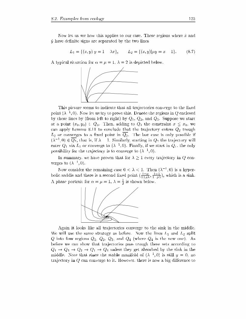
8.2. Examples from ecology 125
Now let us see how this applies to our case. These regions where _x and
_y have de�nite signs are separated by the two lines
L1 = f(x; y)jy = 1� �xg; L2 = f(x; y)j�y = x� 1g: (8.7)
A typical situation for � = � = 1, � = 2 is depicted below.
This picture seems to indicate that all trajectories converge to the �xed
point (��1; 0). Now let us try to prove this. Denote the regions inQ enclosed
by these lines by (from left to right) by Q1, Q2, and Q3. Suppose we start
at a point (x0; y0) 2 Q3. Then, adding to Q3 the constraint x � x0, we
can apply Lemma 8.11 to conclude that the trajectory enters Q2 trough
L2 or converges to a �xed point in Q2. The last case is only possible if
(��1; 0) 2 Q2, that is, if � = 1. Similarly, starting in Q2 the trajectory will
enter Q1 via L1 or converge to (��1; 0). Finally, if we start in Q1, the only
possibility for the trajectory is to converge to (��1; 0).
In summary, we have proven that for � � 1 every trajectory in Q con-
verges to (��1; 0).
Now consider the remaining case 0 < � < 1. Then (��1; 0) is a hyper-
bolic saddle and there is a second �xed point ( 1+�1+�� ;
1��1+�� ), which is a sink.
A phase portrait for � = � = 1, � = 12 is shown below.
Again it looks like all trajectories converge to the sink in the middle.
We will use the same strategy as before. Now the lines L1 and L2 split
Q into four regions Q1, Q2, Q3, and Q4 (where Q4 is the new one). As
before we can show that trajectories pass trough these sets according to
Q4 ! Q3 ! Q2 ! Q1 ! Q4 unless they get absorbed by the sink in the
middle. Note that since the stable manifold of (��1; 0) is still y = 0, no
trajectory in Q can converge to it. However, there is now a big di�erence to
126 8. Planar dynamical systems
the previous case: A trajectory starting in Q4 can return to Q4 and hence
there could be periodic orbits.
To exclude periodic orbits we will try to �nd a Liapunov function. In-
spired by (8.5) we introduce
L(x; y) = y0f(y
y0) + �x0f(
x
x0); (8.8)
where we have abbreviated (x0; y0) = ( 1+�1+�� ;
1��1+�� ) for our �xed point. In
fact, using
_x = (y0 � y � �(x� x0))x; _y = �(x� x0 � �(y � y0))y (8.9)
we compute
_L =@V
@x_x+
@V
@y_y = ���(x� x0)
2 � ��(y � y0)2< 0: (8.10)
Hence we again see that all orbits starting in Q converge to the �xed point
(x0; y0).
Theorem 8.12. Suppose � � 1, then there is no �xed point of the equations
(8.6) in Q and all trajectories in Q converge to the point (0; ��1).
If 0 < � < 1 there is only one �xed point ( 1+�1+�� ;
1��1+��) in Q. It is
asymptotically stable and all trajectories converge to this point.
For our original model this means that the predators can only survive
if their growth rate is positive at the limiting population ��1 of the prey
species.
Problem 8.7. Prove Lemma 8.11.
Problem 8.8 (Volterra principle). Show that for any orbit of the Volterra{
Lotka system (8.3), the time average over one period
1
T
Z T
0
x(t)dt = 1;1
T
Z T
0
y(t)dt = 1
is independent of the orbit. (Hint: Integrate ddt ln(x(t)) over one period.)
Problem 8.9. Show that the change of coordinates x = exp(q), y = exp(p)
transforms the Volterra{Lotka system (8.3) into a Hamiltonian system with
Hamiltonian H(p; q) = L(exp(q); exp(p)).
Moreover, use the same change of coordinates to transform (8.6). Then
use the Bendixson's criterion (Problem 8.4) to show that there are no peri-
odic orbits.
Problem 8.10. Show that (8.6) has no periodic orbits in the case � < 1 if
�� � 1 as follows:

8.3. Examples from electrical engineering 127
If there is a periodic orbit it must contain a point (x0; y0) on L1 which
satis�es1 + �
1 + ��< x0 <
1
�; y0 = 1� �x0: (8.11)
The trajectory enters Q1 and satis�es x(t) < x0 in Q1 since x(t) decreases
there. Hence we must have y(t) < y1 = x0�1� when it hit L2. Now we
enter Q2, where y(t) decreases implying x(t) < x1 =1�y1� when we hit L1.
Proceeding like this we �nally see y(t) > y2 =x1�1� when we return to L1.
If y2 � y0, that is if
(1 + �)(1� ��) � (1� (��)2)x0; (8.12)
the trajectory is spiraling inwards and we get a contradiction to our assump-
tion that it is periodic. This is the case when �� � 1.
Problem 8.11 (Competing species). Suppose you have two species x and
y such that one inhibits the growth of the other. A simple model describing
such a situation would be
_x = (A�By)x
_y = (C �Dx)y; A;B;C;D > 0:
Find out as much as possible about this system.
Problem 8.12 (Competing species with limited growth). Consider the
same setting as in the previous problem but now with limited growth. The
equations read
_x = (1� y � �x)x
_y = �(1 � x� �y)y; �; �; � > 0:
Again, �nd out as much as possible about this system.
8.3. Examples from electrical engineering
An electrical circuit consists of elements each of which has two connectors
(in and out), where every connector of one element is connected to one or
more connectors of the other elements. Mathematically speaking we have
an ordered graph.
At each time t, there will be a certain current I(t) owing through each
element and a certain voltage di�erence V (t) between its connectors. It is
of no importance which connector is called in and which one out. However,
the current is counted positively if it ows from in to out and similarly
for the voltage di�erences. The state space of the system is given by the
pairs (I; V ) of all elements in the circuit. These pairs must satisfy two
requirements. By Kirchho�'s �rst law, the sum over all currents in a vertex
must vanish (conservation of charge) and by Kirchho�'s second law, the
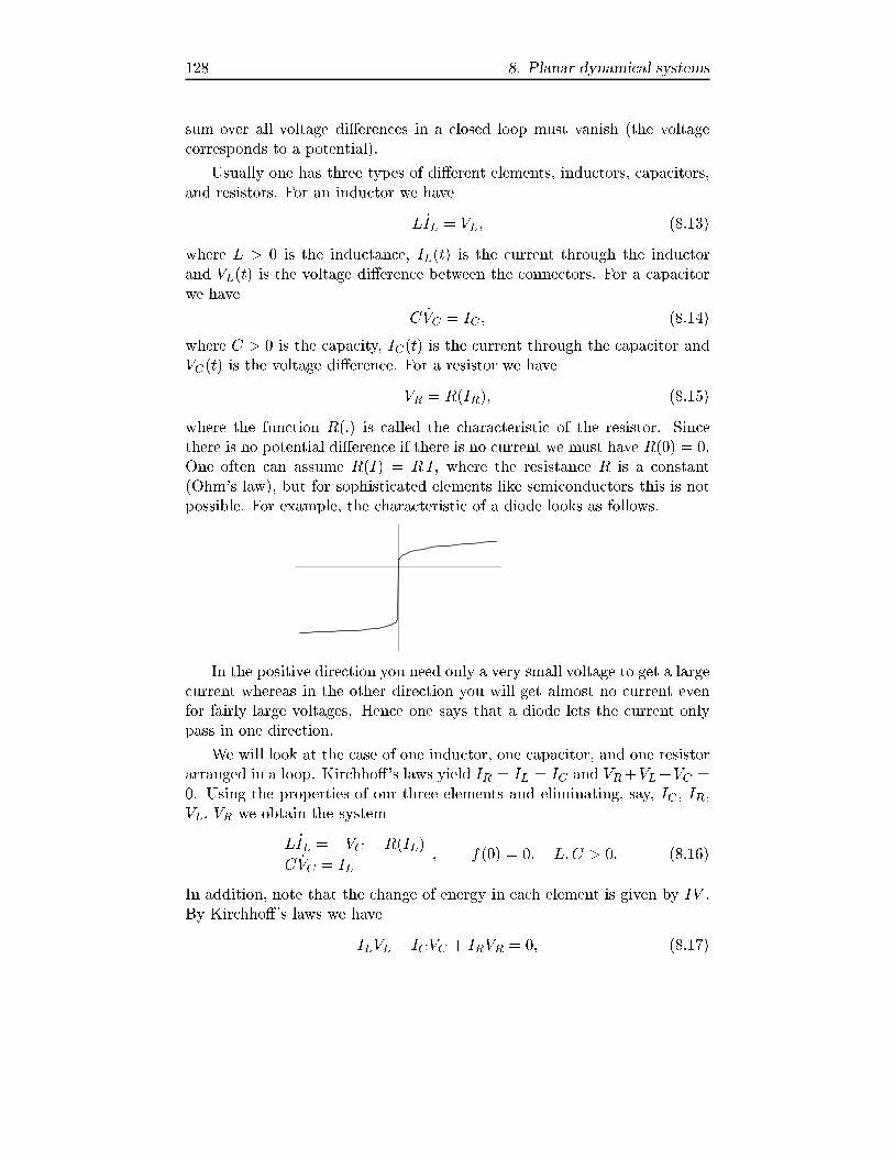
128 8. Planar dynamical systems
sum over all voltage di�erences in a closed loop must vanish (the voltage
corresponds to a potential).
Usually one has three types of di�erent elements, inductors, capacitors,
and resistors. For an inductor we have
L _IL = VL; (8.13)
where L > 0 is the inductance, IL(t) is the current through the inductor
and VL(t) is the voltage di�erence between the connectors. For a capacitor
we have
C _VC = IC ; (8.14)
where C > 0 is the capacity, IC(t) is the current through the capacitor and
VC(t) is the voltage di�erence. For a resistor we have
VR = R(IR); (8.15)
where the function R(:) is called the characteristic of the resistor. Since
there is no potential di�erence if there is no current we must have R(0) = 0.
One often can assume R(I) = RI, where the resistance R is a constant
(Ohm's law), but for sophisticated elements like semiconductors this is not
possible. For example, the characteristic of a diode looks as follows.
In the positive direction you need only a very small voltage to get a large
current whereas in the other direction you will get almost no current even
for fairly large voltages. Hence one says that a diode lets the current only
pass in one direction.
We will look at the case of one inductor, one capacitor, and one resistor
arranged in a loop. Kirchho�'s laws yield IR = IL = IC and VR+VL+VC =
0. Using the properties of our three elements and eliminating, say, IC , IR,
VL, VR we obtain the system
L _IL = �VC �R(IL)
C _VC = IL; f(0) = 0; L; C > 0: (8.16)
In addition, note that the change of energy in each element is given by IV .
By Kirchho�'s laws we have
ILVL + ICVC + IRVR = 0; (8.17)

8.3. Examples from electrical engineering 129
which can be rewritten as
d
dt
�L
2I2L +
C
2V2C
�= �IRR(IR): (8.18)
That is, the energy dissipated in the resistor has to come from the inductor
and the capacitor.
Finally, scaling VC and t we end up with Li�enard's equation (compare
Problem 8.13)
_x = y � f(x)
_y = �x ; f(0) = 0: (8.19)
Equation (8.18) now reads
d
dtW (x; y) = �xf(x); W (x; y) =
x2 + y
2
2: (8.20)
This equation will be our topic for the rest of this section. First of all,
the only �xed point is (0; 0). If xf(x) > 0 in a neighborhood of x = 0, then
W is a Liapunov function and hence (0; 0) is stable. Moreover, we even have
Theorem 8.13. Suppose xf(x) � 0 for all x 2 R and xf(x) > 0 for
0 < jxj < ". then every trajectory of Li�enard's equation (8.19) converges to
(0; 0).
Proof. If W (x; y) is constant on an orbit, say W (x; y) = R2=2, then the
orbit must be a circle of radius R. Hence we must have f(x) = 0 for 0 �jxj � R and the result follows from Liapunov's theorem (Theorem 6.11). �
Conversely, note that (0; 0) is unstable if xf(x) < 0 for 0 < jxj < ".
We will now show that Li�enard's equation has periodic orbits if f is odd
and if xf(x) is negative for x small and positive for x large. More precisely,
we will need the following assumptions.
(i) f is odd, that is, f(�x) = �f(x).(ii) f(x) < 0 for 0 < x < �.
(iii) lim infx!1 f(x) > 0 and in particular f(x) > 0 for x > �.
(iv) f(x) is monotone increasing for x > �.
Furthermore, let us abbreviate Q� = f(x; y)j � x > 0g and L� =
f(x; y)jx = 0;�y > 0g. Our symmetry requirement (i) will allow us to
restrict our attention to Q+ since the corresponding results for Q� will fol-
low via the transformation (x; y) ! (�x;�y) which maps Q+ to Q� and
leave the di�erential equation (8.19) invariant if f is odd.
As a �rst observation we note that
Lemma 8.14. Every trajectory of Li�enard's equation (8.19) in Q+ can cross
the graph of f(x) at most once.

130 8. Planar dynamical systems
Proof. Suppose a trajectory starts below the graph of f , that is y0 < f(x0).
We need to show that it cannot get above again. Suppose at some time t1 we
cross the graph of f . Then y(t1�Æ) < f(x(t1�Æ)) and y(t1+") > f(x(t1+"))
for "; Æ > 0 suÆciently small. Moreover, we must also have x(t1� Æ) > x(t1)
and x(t1+ ") > x(t1) by our di�erential equation. In particular, we can �nd
" and Æ such that x(t1 � Æ) = x(t1 + ") implying
y(t1 + ") > f(x(t1 + ")) = f(x(t1 � Æ)) > y(t1 � Æ): (8.21)
This contradicts that y(t) is decreasing (since x(t) > 0). �
Next we show
Lemma 8.15. Suppose f satis�es the requirements (ii) and (iii). Then,
every trajectory starting at L+ will hit L� at a �nite positive time.
Proof. Suppose we start at (0; y0), y0 > 0. First of all note that the tra-
jectory must satisfy W (x(t); y(t)) � "2=2, where " = minf�; y0g. Next, our
trajectory must hit the line f(x; y)jx = �; y > 0g by Lemma 8.11. Moving
on we must hit f(x; y)jx > 0; y = 0g. Otherwise we would have x(t) ! 1in �nite time (since _y(t) � �) which is impossible since _x(t) � y0. But from
this point on we must stay within the region x(t) � R and x2+(y�C)2 � R2,
where R > � is suÆciently large and C < inf f(x). This follows since the
vector �eld always points to the interior of this region. Applying again
Lemma 8.11 �nishes the proof. �
Now suppose f satis�es (i){(iv). Denote the �rst intersection point of the
trajectory starting at (x(0); y(0)) = (0; y0) 2 L+ with L� by (x(T ); y(T )) =
(0; P (y0)). Then, every periodic orbit orbit must encircle (0; 0) and satisfy
P (y0) = �y0. Hence every periodic orbit corresponds to a zero of the
function
�(y0) =W (0; P (y0))�W (0; y0) = �Z T
0
x(t)f(x(t))dt: (8.22)
Now what can we say about this function? Clearly, for y0 < � we have
�(y0) > 0. Moreover, there is a number r > 0 such that the trajectory
starting at (0; r) intersects the graph at (�; 0) (show this). So for y0 > r
our trajectory intersects the line x = � at t1 and t2. Furthermore, since the
intersection with f can only be for t 2 (t1; t2), we have y(t) > f(x(t)) for
0 � t � t1 and y(t) < f(x(t)) for t2 � t � T . Now let us split � into three
parts by splitting the integral at t1 and t2. For the �rst part we obtain
�1(y0) = �Z t1
0
x(t)f(x(t))dt =
Z �
0
�xf(x)y(x)� f(x)
dx: (8.23)
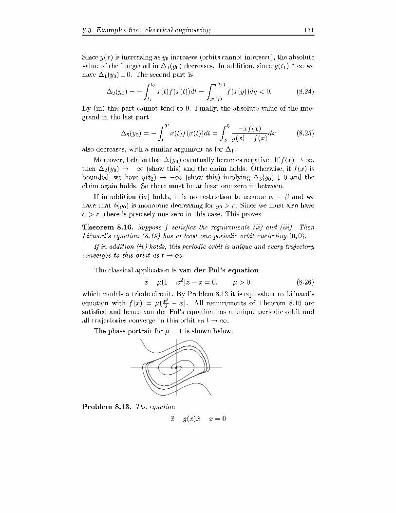
8.3. Examples from electrical engineering 131
Since y(x) is increasing as y0 increases (orbits cannot intersect), the absolute
value of the integrand in �1(y0) decreases. In addition, since y(t1) " 1 we
have �1(y0) # 0. The second part is
�2(y0) = �Z t2
t1
x(t)f(x(t))dt =
Z y(t2)
y(t1)f(x(y))dy < 0: (8.24)
By (iii) this part cannot tend to 0. Finally, the absolute value of the inte-
grand in the last part
�3(y0) = �Z T
t1
x(t)f(x(t))dt =
Z 0
�
�xf(x)y(x)� f(x)
dx (8.25)
also decreases, with a similar argument as for �1.
Moreover, I claim that �(y0) eventually becomes negative. If f(x)!1,
then �2(y0) ! �1 (show this) and the claim holds. Otherwise, if f(x) is
bounded, we have y(t2) ! �1 (show this) implying �3(y0) # 0 and the
claim again holds. So there must be at least one zero in between.
If in addition (iv) holds, it is no restriction to assume � = � and we
have that Æ(y0) is monotone decreasing for y0 > r. Since we must also have
� > r, there is precisely one zero in this case. This proves
Theorem 8.16. Suppose f satis�es the requirements (ii) and (iii). Then
Li�enard's equation (8.19) has at least one periodic orbit encircling (0; 0).
If in addition (iv) holds, this periodic orbit is unique and every trajectory
converges to this orbit as t!1.
The classical application is van der Pol's equation
�x� �(1� x2) _x+ x = 0; � > 0; (8.26)
which models a triode circuit. By Problem 8.13 it is equivalent to Li�enard's
equation with f(x) = �(x3
3� x). All requirements of Theorem 8.16 are
satis�ed and hence van der Pol's equation has a unique periodic orbit and
all trajectories converge to this orbit as t!1.
The phase portrait for � = 1 is shown below.
Problem 8.13. The equation
�x+ g(x) _x+ x = 0

132 8. Planar dynamical systems
is also often called Li�enard's equation. Show that it is equivalent to (8.19)
if we set y = _x+ f(x), where f(x) =R x0 g(t)dt.
Chapter 9
Higher dimensional
dynamical systems
9.1. Attracting sets
In most applications, the main interest is to understand the long time be-
havior of the ow of a di�erential equation (which we assume � complete
from now on for simplicity). In this respect it is important to understand
the fate of all points starting in some set X. Hence we will extend some of
our previous de�nitions to sets �rst.
Given a set X �M we can always obtain a � invariant set by considering
�(X) =[�t�0
�(t;X) =[x2X
�(x): (9.1)
Taking the closure �(X) we even obtain a closed � invariant set. Moreover,
the !�-limit set of X is the set !�(X) of all points y 2M for which there
exists sequences tn ! �1 and xn 2 X with �(tn; xn)! y.
We will only consider the case � = + from now on for notational sim-
plicity. The set !+(X) can equivalently be characterized as,
!+(X) =\t�0
�(t; +(X)) =\t�0
[s�t
�(s;X): (9.2)
Clearly, !+(X) is closed as the intersection of closed sets and it is also not
hard to see that is invariant (Problem 9.1).
Lemma 9.1. The set !�(X) is a closed invariant set.
133

134 9. Higher dimensional dynamical systems
In addition, by �(t; +(X)) � +(X) we have �(s; +(X)) � �(t; +(X))
for s > t and hence it is immediate that
!+(X) =\t�t0
�(t; +(X)) =\n2N
�(n; +(X)): (9.3)
So if +(X) 6= ; is compact, !+(X) is the intersection of countably many
nonempty compact nesting sets and thus it is also a nonempty compact set
by the �nite intersection property of compact sets.
Lemma 9.2. Suppose X is nonempty. If the set �(X) is compact, then
!�(X) is nonempty and compact. If �(X) is in addition connected (e.g., if
X is connected), then so is !�(X).
Proof. It remains to show that � = !+(X) is connected. Suppose it is not
and can be split into two disjoint closed sets, � = �0 [�1, none of which is
empty. Since Rn is normal, there are disjoint open sets U0 and U1 such that
�0 � U0 and �1 � U1. Moreover, the set Vn = �(n; +(X))n(U0 [ U1) iscompact. Hence V =
Tn Vn is either nonempty or Vn is eventually empty. In
the �rst case we must have V � � which is impossible since V \(U0[U1) = ;.Otherwise, if Vn is eventually empty, then �(n; +(X)) must be eventually
in U0 or in U1 (since �(n; +(X)) is connected) implying � � U0 respectively
� � U1. Again a contradiction. �
Note that we have [x2X
!+(x) � !+(X) (9.4)
but equality will not hold in general as the example
_x = x(1� x2); _y = �y (9.5)
shows. In this case it is not hard to see that
!+(Br(0)) = [�1; 1] � f0g; r > 1; (9.6)
but [x2Br(0)
!+(x) = f(�1; 0); (0; 0); (1; 0)g: (9.7)
In particular !+(Br(0)) contains the three �xed points plus their unstable
manifolds. That is, all orbits which lie entirely in Br(0). This is also true
in general.
Theorem 9.3. The set !+(X) is the union over all complete orbits lying
entirely in +(X).
Proof. Let (y) be such a orbit, then (y) � +(X) and invariance of (y)
implies (y) � �(t; +(X)) for all t and hence (y) � !+(X). The converse
follows since !+(X) � +(X). �

9.1. Attracting sets 135
An invariant set � is called attracting if there exists some neighborhood
U of � such that U is positively invariant and �t(x) ! � as t! 1 for all
x 2 U . The setsW
�(�) = fx 2M j limt!�1
d(�t(x);�) = 0g (9.8)
are the stable respectively unstable sets of �. Here d(A;B) = inffjx �yj jx 2 A; y 2 Bg denotes the distance between two sets A;B � R
n . The set
W+(�) is also called the domain or basin of attraction for �. It is not
hard to see that we have
W+(�) =
[t<0
�t(U) = fx 2M j!+(x) � �g: (9.9)
But how can we �nd such a set? Fortunately, using our considerations
from above, there is an easy way of doing so. An open connected set E whose
closure is compact is called a trapping region for the ow if �t(E) � E,
t > 0. In this case
� = !+(E) =\t�0
�(t; E) (9.10)
is an attracting set by construction.
Unfortunately the de�nition of an attracting set is not always good
enough. In our example (9.5) any ball Br(0) with radius r > 1 is a trapping
region. However, whereas only the two �xed points (�1; 0) are really attract-ing, the corresponding attracting set � also contains the repelling �xed point
(0; 0) plus its unstable manifold. In particular, the domain of attraction of
the two attracting �xed points W+(f(�1; 0); (1; 0)g) = f(x; y) 2 R2 jx = 0g
is up to a set of measure zero the same as W+(�) = R2 .
In fact, an attracting set will always contain the unstable manifolds of
all its points.
Lemma 9.4. Let E be a trapping region, then
W�(x) � !+(E); 8x 2 !+(E): (9.11)
Proof. From y 2 W�(x) we infer �(t; y) 2 +(E) for t ! �1. Hence
(y) � +(E) and the claim follows from Theorem 9.3. �
To exclude such situations, we can de�ne an attractor to be an attract-
ing set which is topologically transitive. Here a closed invariant set � is
called topologically transitive if for any two open sets U; V � � there is
some t 2 R such that �(t; U)\V 6= ;. In particular, an attractor cannot be
split into smaller attracting sets. Note that � is topologically transitive if
it contains a dense orbit (Problem 9.2).

136 9. Higher dimensional dynamical systems
This implies that only the sets f(�1; 0)g or f(1; 0)g are attractors for theabove example. The domains of attraction are W+(f(�1; 0)g) = f(x; y) 2R2 j � x > 0g.As another example let us look at the DuÆng equation
�x = �Æ _x+ x� x3; Æ � 0; (9.12)
from Problem 6.17. It has a sink at (�1; 0), a hyperbolic saddle at (0; 0),
and a sink at (1; 0). The basin of attraction of the sink (�1; 0) is boundedby the stable and unstable manifolds of the hyperbolic saddle (0; 0). The
situation for Æ = 0:3 is depicted below.
Finally, let us consider the van der Pol equation (8.26). The unique
periodic orbit is an attractor and its basin of attraction is R2nf0g. However,not all attractors are �xed points or periodic orbits, as the example in our
next section will show.
Problem 9.1. Show that !�(X) is invariant under the ow.
Problem 9.2. Show that a closed invariant set which has a dense orbit is
topologically transitive.
9.2. The Lorenz equation
One of the most famous dynamical systems which exhibits chaotic behavior
is the Lorenz equation
_x = ��(x� y);
_y = rx� y � xz;
_z = xy � bz; (9.13)
where �; r; b > 0. Lorenz arrived at these equations when modelling a two-
dimensional uid cell between two parallel plates which are at di�erent tem-
peratures. The corresponding situation is described by a complicated system
of nonlinear partial di�erential equations. To simplify the problem, he ex-
panded the unknown functions into Fourier series with respect to the spacial
coordinates and set all coeÆcients except for three equal to zero. The result-
ing equation for the three time dependent coeÆcients is (9.13). The variable
x is proportional to the intensity of convective motion, y is proportional to

9.2. The Lorenz equation 137
the temperature di�erence between ascending and descending currents, and
z is proportional to the distortion from linearity of the vertical temperature
pro�le.
So let us start with an investigation of this system. First of all observe
that the system is invariant under the transformation
(x; y; z)! (�x;�y; z): (9.14)
Moreover, the z axis is an invariant manifold since
x(t) = 0; y(t) = 0; z(t) = z0e�bt (9.15)
is a solution of our system.
But now let us come to some deeper results. We �rst show that the
dynamic is quite simple if r � 1. If r � 1 there is only one �xed point of
the vector �eld, namely the origin. The linearization is given by0@ �� � 0
r �1 0
0 0 �b
1A (9.16)
and the corresponding eigenvalues are
�b; �1
2(1 + � �
p(1 + �)2 + 4(r � 1)�): (9.17)
Hence the origin is asymptotically stable for r < 1. Moreover, it is not hard
to see that
L(x; y; z) = rx2 + �y
2 + �z2 (9.18)
is a Liapunov function in this case since one readily veri�es
_L(x; y; z) = ��(r(x+ y)2 + (1� r)y2 + bz2): (9.19)
In particular, the following lemma follows easily from Theorem 6.11 (Prob-
lem 9.3).
Lemma 9.5. Suppose r � 1, then the Lorenz equation has only the origin
as �xed point and all solutions converge to the origin as t!1.
If r grows above 1, there are two new �xed points
(x; y; z) = (�pb(r � 1);�
pb(r � 1); r � 1); (9.20)
and the linearization is given by0@ �� � 0
1 �1 �pb(r � 1)
�pb(r � 1) �
pb(r � 1) �b
1A : (9.21)
One can again compute the eigenvalues but the result would almost �ll one
page. Note however that by (9.14) the eigenvalues are the same for both
points. From (9.17) we can read o� that one eigenvalue is now positive and
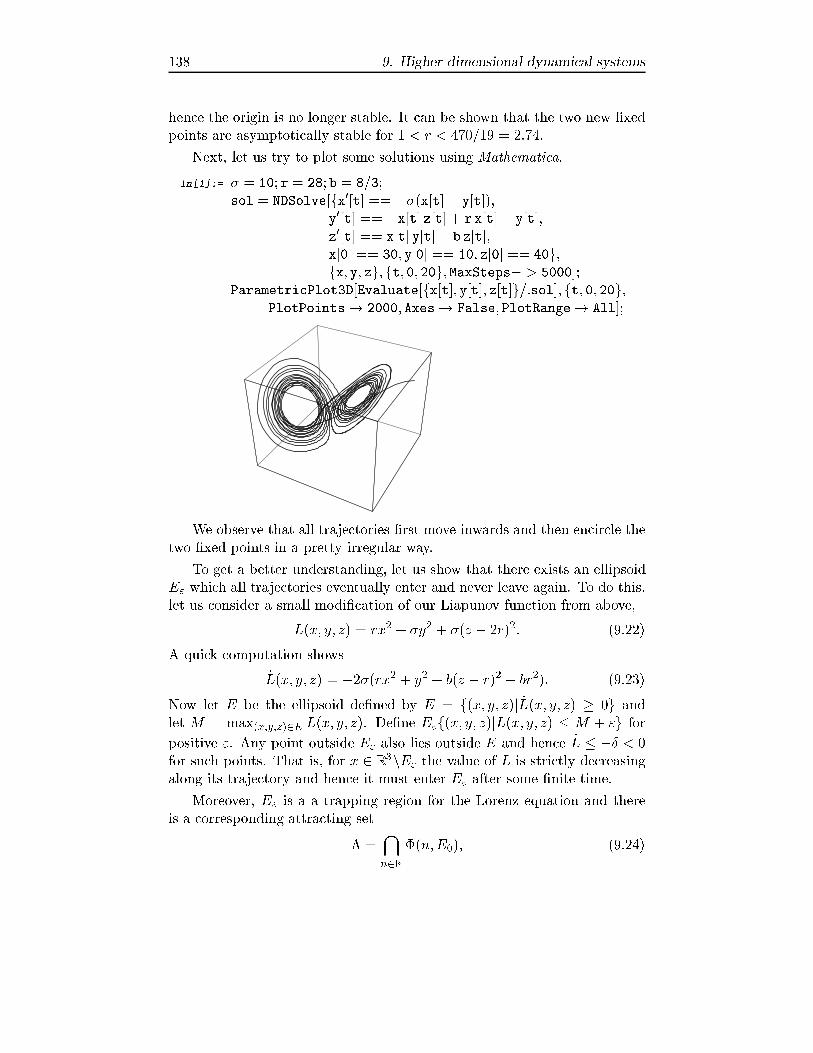
138 9. Higher dimensional dynamical systems
hence the origin is no longer stable. It can be shown that the two new �xed
points are asymptotically stable for 1 < r < 470=19 = 2:74.
Next, let us try to plot some solutions using Mathematica.
In[1]:= � = 10; r = 28; b = 8=3;
sol = NDSolve[fx0[t] == ��(x[t]� y[t]);
y0[t] == �x[t] z[t] + r x[t]� y[t];
z0[t] == x[t] y[t]� b z[t];
x[0] == 30; y[0] == 10; z[0] == 40g;fx; y; zg; ft; 0; 20g; MaxSteps� > 5000];
ParametricPlot3D[Evaluate[fx[t]; y[t]; z[t]g=:sol]; ft; 0; 20g;PlotPoints! 2000; Axes! False; PlotRange! All];
We observe that all trajectories �rst move inwards and then encircle the
two �xed points in a pretty irregular way.
To get a better understanding, let us show that there exists an ellipsoid
E" which all trajectories eventually enter and never leave again. To do this,
let us consider a small modi�cation of our Liapunov function from above,
L(x; y; z) = rx2 + �y
2 + �(z � 2r)2: (9.22)
A quick computation shows
_L(x; y; z) = �2�(rx2 + y2 + b(z � r)2 � br
2): (9.23)
Now let E be the ellipsoid de�ned by E = f(x; y; z)j _L(x; y; z) � 0g and
let M = max(x;y;z)2E L(x; y; z). De�ne E"f(x; y; z)jL(x; y; z) � M + "g for
positive ". Any point outside E" also lies outside E and hence _L � �Æ < 0
for such points. That is, for x 2 R3nE" the value of L is strictly decreasing
along its trajectory and hence it must enter E" after some �nite time.
Moreover, E" is a a trapping region for the Lorenz equation and there
is a corresponding attracting set
� =\n2N
�(n;E0); (9.24)

9.2. The Lorenz equation 139
which is called the attractor of the Lorenz equation. In particular, we see
that solutions exist for all positive times. Note also that W+(�) = R3 . All
�xed points plus their unstable manifolds (if any) must also be contained in
�. Moreover, I even claim that � is of Lebesgue measure zero. To see this
we need a generalized version of Liouville's formula (3.39).
Lemma 9.6. Let _x = f(x) be a dynamical system on Rn with corresponding
ow �(t; x). Let M be a bounded measurable subset of Rn and let V =RM dx
be its volume. Abbreviate M(t) = �(t;M) respectively V (t) =RM(t) dx, then
_V (t) =
ZM(t)
div(f(x)) dx: (9.25)
Proof. By the change of variable formula for multiple integrals we have
V (t) =
ZM(t)
dx =
ZMdet(d�t(x)) dx: (9.26)
Since d�t = I+ df t + o(t) we infer V (t) =RM (1 + tr(df)t + o(t)) dx and
hence
_V (0) = limt!0
V (t)� V (0)
t= lim
t!0
ZM(tr(df) + o(1)) dx =
ZMtr(df) dx (9.27)
by the dominated convergence theorem. ReplacingM withM(t) shows that
the above result holds for all t and not only for t = 0. �
Applying this lemma to the Lorenz equation we obtain
V (t) = V e�(1+�+b)t (9.28)
since
div(f) = �(1 + � + b): (9.29)
In particular, we see that the measure of �(t; E0) decreases exponentially,
and the measure of � must be zero. Note that this result also implies that
none of the three �xed points can be a source.
Our numerical experiments from above show that � seems to be a quite
complicated set. This is why it was called the strange attractor of the
Lorenz equation.
However, this is clearly no satisfying mathematical de�nition of a strange
attractor. One possibility is to call an attractor strange if the dynamical
system generated by the time-one map
�1 : �! � (9.30)
is chaotic and if � is fractal. It is still unknown whether the Lorenz attractor
is strange in the sense of this de�nition. See the book by Sparrow [26] for a
survey of results.

140 9. Higher dimensional dynamical systems
I will not go into any further details at this point. We will see how these
terms are de�ned in Section 12.3 and Section 12.6, respectively. However,
I hope that this example shows that even simple systems in R3 can exhibit
very complicated dynamics. I also hope that you can now better appreciate
the Poincar�e{Bendixson which excludes such strange behavior in R2 .
Problem 9.3. Prove Lemma 9.5.
Problem 9.4. Solve the Lorenz equation for the case � = 0.
Problem 9.5. Investigate the Lorenz equation for the case r =1 as follows.
First introduce " = r�1. Then use the change of coordinates (t; x; y; x) 7!
(�; �; �; �), where � = "�1t, � = "x, � = �"
2y, and � = �("2z � 1).
Show that the resulting system for " = 0 corresponds to a single third
order equation �000 = ��2�0. Integrate this equation once and observe that
the result is of Newton type (see Section 6.6). Now what can you say about
the solutions?
9.3. Hamiltonian mechanics
In the previous sections we have seen that even simple looking dynamical
systems in three dimension can be extremely complicated. In the rest of this
chapter we want to show that it is still possible to get some further insight
if the system has a special structure. Hence we will look again at systems
arising in classical mechanics.
The point of departure in classical mechanics is usually the Hamilton
principle. Suppose a mechanical system has n degrees of freedom described
by coordinates q 2 U � Rn . Associated with such a system is a Lagrange
function
L(v; q); v = _q; (9.31)
and an integral curve q(t) for which the action integral
I(q) =Z t1
t0
L( _q(t); q(t))dt (9.32)
subject to the boundary conditions q(t0) = q0, q(t1) = q1 is extremal.
If L is di�erentiable, extremal curves can be found by setting the Gateaux
derivative of I equal to zero. That is, setting
q"(t) = q(t) + "r(t); (9.33)
we see that a necessary condition for q to be extremal is that
d
d"I(q")
���"=0
= 0: (9.34)
9.3. Hamiltonian mechanics 141
Using integration by parts this immediately yields (Problem 9.6) the corre-
sponding Euler-Lagrange equation
@L
@q� d
dt
@L
@v= 0: (9.35)
In the situation of particles under the in uence of some forces we have
L(v; q) =1
2vMv � U(q); (9.36)
where M is a positive diagonal matrix with the masses of the particles as
entries and U is the potential corresponding to the forces. The associated
Euler-Lagrange equations are just Newton's equations
M �q = �gradU(q): (9.37)
If the momentum
p(v; q) =@L
@v(v; q) (9.38)
is a di�eomorphism for �xed q, and hence
det@2L
@v26= 0; (9.39)
then we can consider the Legendre transform of L,
H(p; q) = pv � L(v; q); v = v(p; q); (9.40)
which is known as the Hamilton function of the system. The associated
variational principle is that the integral
I(p; q) =Z t1
t0
�p(t) _q(t)�H(p(t); q(t))
�dt (9.41)
subject to the boundary conditions q(t0) = q0, q(t1) = q1 is extremal. The
corresponding Euler-Lagrange equations are Hamilton's equations
_q =@H(p; q)
@p; _p = �@H(p; q)
@q: (9.42)
This formalism is called Hamilton mechanics.
In the special case of some particles we have
p =Mv; H(p; q) =1
2pM
�1p+ U(q) (9.43)
and the Hamiltonian corresponds to the total energy of the system.
Introducing the symplectic matrix
J =
�0 I
�I 0
�; J
�1 = JT = �J; (9.44)

142 9. Higher dimensional dynamical systems
Hamilton's equation can also be written as
d
dt
�p
q
�= �gradsH(p; q) = �J gradH(p; q); (9.45)
where grads is called the symplectic gradient.
A straightforward calculation shows that H is a constant of motion,
that is,
d
dtH(p(t); q(t)) =
@H
@p_p+
@H
@q_q = �@H
@p
@H
@q+@H
@q
@H
@p= 0: (9.46)
More generally, for a function I(p; q) its change along a trajectory is given
by its Lie derivative (compare (6.41))
d
dtI(p(t); q(t)) = fI(p(t); q(t));H(p(t); q(t))g; (9.47)
where
fI;Hg = @I
@p
@H
@q� @I
@q
@H
@p(9.48)
is called Poisson bracket. This should be compared with the Heisenberg
equation of Problem 3.8.
A function I(p; q) is called a �rst integral if it is constant along tra-
jectories, that is, if
fI;Hg = 0: (9.49)
But how can we �nd �rst integrals? One source are symmetries.
Theorem 9.7 (Noether). Let �(t; q) be the ow generated by f(q). If �
leaves the Lagrangian invariant, then
I(v; q) =@L(v; q)
@vf(q) (9.50)
is a constant of motion.
Proof. Abbreviate qs(t) = �(s; q(t)). The invariance of L(v; q) implies
0 =d
dsL( _qs(t); qs(t))
���s=0
=@L
@v( _q(t); q(t))
@f
@q(q(t)) _q(t) +
@L
@q( _q(t); q(t))f(q(t)) (9.51)
and hence
d
dtI( _q(t); q(t)) =
�d
dt
@L
@v( _q; q)
�f(q) +
@L
@v( _q; q)
@f
@q(q) _q
=
�d
dt
@L
@v( _q; q)� @L
@q( _q; q)
�f(q) = 0 (9.52)
by the Euler-Lagrange equation. �

9.3. Hamiltonian mechanics 143
Another important property of Hamiltonian systems is that they are
volume preserving. This follows immediately form Lemma 9.6 since the
divergence of a Hamiltonian vector �eld is zero.
Theorem 9.8 (Liouville). The volume in phase space is preserved under a
Hamiltonian ow.
This property can often give important information concerning the mo-
tion via Poincar�e's recurrence theorem.
Theorem 9.9 (Poincar�e). Suppose � is a volume preserving bijection of a
bounded region D � Rn . Then in any neighborhood U � D there is a point
x returning to U , that is, �n(x) 2 U for some n 2 N.
Proof. Consider the sequence �n(U) � D. There are two numbers l, k such
that �l(U)\�k(U) 6= ; since otherwise their volume would be in�nite. HenceU \ �k�l(U) 6= ;. If y is a point in the intersection we have y = �k�l(x),
which proves the claim. �
Problem 9.6. Derive the Euler-Lagrange equation (9.35).
Problem 9.7 (Legendre transform). Let F (v) be such that
det@2F
@v2(v0) 6= 0:
Show that the function p(v) = @F@v (v) is a local di�eomorphism near v0 and
that the Legendre transform
G(p) = pv(p)� F (v(p))
is well de�ned. Show that
p =@F
@v(v) , v =
@G
@p(p)
and conclude that the Legendre transformation is involutive.
Problem 9.8. Suppose that D is positively invarant under a volume pre-
serving ow. Then D belongs to the set of nonwandering points. (Hint: The
Poincar�e's recurrence theorem and Problem 6.8.)
Problem 9.9 (Relativistic mechanics). Einstein's equation says that the
kinetic energy of a relativistic particle is given by
T (v) = m(v)c2; m(v) = m0
r1 +
v2
c2;
where c is the speed of light and m0 is the (rest) mass of the particle. De-
rive the equation of motions from Hamilton's principle using the Lagrangian
L(v; q) = T (v)� U(q). Derive the corresponding Hamilton equations.
144 9. Higher dimensional dynamical systems
9.4. Completely integrable Hamiltonian systems
Finally we want to show that there is also a canonical form for a Hamil-
ton system under certain circumstances. To do this we need to transform
our system in such a way that the Hamilton structure is preserved. More
precisely, if our transformation is given by
(P;Q) = '(p; q); (p; q) = (P;Q); (9.53)
we have�_P_Q
�= d'
�_p
_q
�= �d'J gradH(p; q) = �(d'Jd'T ) gradK(P;Q);
(9.54)
whereK = H Æ' is the transformed Hamiltonian. Hence, we need to require
that the Jacobian of ' is a symplectic matrix, that is,
d' 2 Sp(2n) = fM 2 Gl(2n)jMJMT = Jg; (9.55)
where Sp(2n) is the symplectic group. Such a map is called a symplectic
map. In this case ' is also called a canonical transform. Alternatively
they can be characterized as those transformations which leave the sym-
plectic two form
!((p1; q1); (p2; q2)) = (p1; q1)J(p2; q2) = p1q2 � p2q1 (9.56)
invariant.
To �nd canonical transformations, recall that we have derived Hamil-
ton's equations from the variational principle (9.41). Hence, our transform
will be canonical if the integrands of (9.41) and
~I(P;Q) =
Z t1
t0
P (t) _Q(t)�K(P (t); Q(t))dt (9.57)
only di�er by a total di�erential. By H(p; q) = K(P;Q) we are lead to
pdq � PdQ = dS; (9.58)
where dq has to be understood as dq(t) = _q(t)dt for a given curve q(t).
The function S is called a generating function and could depend on all four
variables p, q, P , and Q. However, since only two of them are independent
in general, it is more natural to express two of them by the others.
For example, we could use
S = S1(q;Q) (9.59)
and
pdq � PdQ =@S1
@qdq +
@S1
@QdQ (9.60)
9.4. Completely integrable Hamiltonian systems 145
shows we have
p =@S1
@q; P = �@S1
@Q; (9.61)
since the previous equation must hold for all curves q(t) and Q(t). Moreover,
if we require
det@S1
@q@Q6= 0; (9.62)
we can solve p =@S1(q;Q)
@q locally for Q = Q(p; q) and hence our canonical
transformation is given by
(P;Q) = (@S1
@Q(q;Q(p; q)); Q(p; q)): (9.63)
Similarly we could choose
S = �PQ+ S2(P; q); (9.64)
where
pdq � PdQ = �QdP � PdQ+@S2
@PdP +
@S2
@QdQ (9.65)
implies
Q =@S2
@P; p =
@S2
@q: (9.66)
Again, if we require
det@S2
@P@q6= 0; (9.67)
we obtain a canonical transformation
(P;Q) = (P (p; q);@S2
@P(P (p; q); q)): (9.68)
The remaining two cases
S = qp+ S3(Q; p) and S = qp� PQ+ S4(P; p) (9.69)
are left as an exercise.
Now let us return to our canonical form. We will start with one dimen-
sion, that is, n = 1 with H(p; q) as in (6.52). Let q0 be a local minimum
of U(q) surrounded by periodic orbits E which are uniquely determined by
the energy E of a point on the orbit. The two intersection points of E with
the q axis to the left and right of q0 will be denoted by q�(E) and q+(E),
respectively.
The integral over the momentum along such a periodic orbit
I(E) =1
2�
Z E
p dq =1
�
Z q+(E)
q�(E)
p2(E � U(q))dq (9.70)

146 9. Higher dimensional dynamical systems
is called the action variable. Next, by (6.47)
I0(E) =
1
�
Z q+(E)
q�(E)
dqp2(E � U(q))
=T (E)
2�> 0; (9.71)
where T (E) is the period of E , and thus we can express E as a function of
I, say E = K(I). Hence if we take I as one of our new variables, the new
Hamiltonian K will depend on I only. To �nd a suitable second variable we
will look for a generating function S2(I; q). Since we want p =@S2@q we set
S2(I; q) =
Z q
q�(K(I))
pdq =1
�
Z q
q�(K(I))
p2(K(I)� U(q))dq (9.72)
and the second variable is
� =@S2
@I=
Z q
q�(E)
I0(E)�1dqp2(E � U(q))
=2�
T (E)t; (9.73)
where t is the time it takes from q�(E) to q (compare again (6.47)). The
variable � is called the angle variable and is only de�ned modulo 2�. The
equation of motion read
_I = �@K@�
= 0;
_� =@K
@I= (I); (9.74)
where (I) = 2�=T (K(I)).
The main reason why we could �nd such a canonical transform to action-
angle variables is the existence of a �rst integral, namely the Hamiltonian.
In one dimension this single �rst integral suÆces to decompose the surfaces
of constant energy into periodic orbits. In higher dimensions this is no longer
true unless one can �nd n �rst integrals Lj which are functionally indepen-
dent and in involution, fLj; Lkg = 0. Such systems are called completely
integrable. If the system is integrable, the n �rst integrals can be used to
de�ne the n-dimensional manifolds �c = f(p; q)jLj(p; q) = cj ; 1 � j � ngwhich can be shown to be di�eomorphic to an n-dimensional torus (if they
are compact). Taking a basis of cycles f j(c)gnj=1 on the torus �c one can
de�ne the action variables as before via
Ij(c) =1
2�
Z j(c)
p dq (9.75)
and the angle variables via a generating function S2(I; q) =R qp dq. I do not
want to go into further details here but I refer to the excellent book by Arnold
[2]. However, I will at least illustrate the situation for the prototypical

9.4. Completely integrable Hamiltonian systems 147
example. Approximating the potential U(q) near a local minimum we obtain
U(q) = U(q0) +1
2qWq + o(jqj2); (9.76)
where W is a positive matrix and U(q0) can be chosen zero. Neglecting the
higher order terms, the resulting model
H(p; q) =1
2(pMp+ qWq) (9.77)
is known as harmonic oscillator. Let V be the (real) orthogonal matrix
which transforms the symmetric matrix M�1=2WM
�1=2 to diagonal form
and let !2j be the eigenvalues. Then the symplectic transform (P;Q) =
(VM1=2p; V M
�1=2q) (Problem 9.11) gives the decoupled system
_Qj = Pj ;_Pj = �!2jQj; j = 1; : : : ; n: (9.78)
In particular,
K(P;Q) =
nXj=1
Kj ; Kj =1
2(P 2
j +Q2j ); (9.79)
where the Kj 's are n �rst integrals in involution (check this). The corre-
sponding action-angle variables are given by (Problem 9.13)
Ij =1
2(P2j
!j+ !jQ
2j); �j = arccot
Pj
!jQj: (9.80)
For example, consider the following Hamiltonian
H(p; q) =
nXj=1
pj
2m+ U0 (qj+1 � qj) ; q0 = qn+1 = 0 (9.81)
which describes a lattice of equal n particles (with mass m) with nearest
neighbor interaction described by the potential U0(x). The zeroth and n-th
particle are considered �xed and qj is the displacement of the j-th particle
from its equilibrium position. If we assume that the particles are coupled
by springs, the potential would be U0(x) =k2x
2, where k > 0 is the so called
spring constant, and we have a harmonic oscillator. The motion is decom-
posed into n modes corresponding to the eigenvectors of the Jacobian of the
potential. Physicists believed for a long time that a nonlinear perturbation
of the force will lead to thermalization. That is, if the system starts in a
certain mode of the linearized system, the energy will eventually be dis-
tributed equally over all modes. However, Fermi, Pasta, and Ulam showed
with computer experiments that this is not true (Problem 9.14). This is
related to the existence of solitons, see for example [19].
Problem 9.10 (Symplectic group). Show that Sp(2n) is indeed a group.
Suppose M 2 Sp(2n), show that det(M)2 = 1 and �M (z) = �M (z�1).
148 9. Higher dimensional dynamical systems
Problem 9.11. Show that the transformation (P;Q) = (Up; (U�1)T q),
where U is an arbitrary matrix, is canonical.
Problem 9.12. Show that the transformation generated by a function S is
canonical by directly proving that d' is symplectic. (Hint: Prove �Jd' =
Jd T using
@p
@Q=
@2S1
@Q@q= �
�@P
@q
�Tand similar for the others.)
Problem 9.13. Consider the harmonic oscillator in one dimension
H(p; q) =1
2p2 +
!2
2q2
and show that S1(q; �) =!2 q
2 cot(�) generates a canonical transformation to
action-angle variables.
Problem 9.14 (Fermi-Pasta-Ulam experiment). Consider the Hamiltonian
(9.81) with the interaction potential U0(x) =k2(x2 + �x
3). Note that it is
no restriction to use m = k = 1 (why?).
Compute the eigenvalues and the eigenvectors of the linearized system
� = 0. Choose an initial condition in an eigenspace and (numerically)
compute the time evolution. Investigate how the state is distributed with
respect to the eigenvectors as a function of t. (Choose N = 32, � = 1=6.)
Problem 9.15. Show that the Poisson bracket satis�es the Jacobi identity
fI; fJ;Kgg + fJ; fK; Igg + fK; fI; Jgg = 0
and Leibniz' rule
fI; J Kg = JfI;Kg +KfI; Jg:
Problem 9.16 (Lax pair). Let L(p; q) and P (p; q) be n by n matrices. They
are said to form a Lax pair for a Hamiltonian system if the equations of
motion (9.42) are equivalent to the Lax equation
_L = [P;L]:
Show that the quantities
tr(Lj); 1 � j � n;
are �rst integrals (Hint: Compare Problem 3.8).

9.5. The Kepler problem 149
9.5. The Kepler problem
Finally, as an application of our results we will show how to solve equation
(1.11) from Section 1.1. In fact, we will even consider a slightly more general
case, the two body problem. Suppose we have two masses placed at
x1 2 R3 and x2 2 R
3 . They interact with a force F depending only on the
distance of the masses and lies on the line connecting both particles. The
kinetic energy is given by
T ( _x) =m1
2_x21 +
m2
2_x22 (9.82)
and the potential energy is
U(x) = U(jx1 � x2j): (9.83)
The Lagrangian is the di�erence of both
L( _x; x) = T ( _x)� U(x): (9.84)
Clearly it is invariant under translations (x1; x2) 7! (x1+sa; x2+sa), a 2 R3 ,
and so Theorem 9.7 tells us that all three components of the total momentum
m1 _x1 +m2 _x2 (9.85)
are �rst integrals. Hence we will choose new coordinates
q1 =m1x1 +m2x2
m1 +m2; q2 = x1 � x2 (9.86)
in which our Lagrangian reads
L( _q; q) =M
2_q21 +
�
2_q22 � U(q2); M = m1 +m2; � =
m1m2
M: (9.87)
In particular, the system decouples and the solution of the �rst part is given
by q1(t) = q1(0) + _q1(0)t. To solve the second, observe that it is invariant
under rotations and, invoking again Theorem 9.7, we infer that the angular
momentum
l = �q2 ^ _q2 (9.88)
is another �rst integral. Hence we have found three �rst integrals and we
suspect that our system is integrable. However, since
fl1; l2g = l3; fl1; l3g = �l2; fl2; l3g = l1 (9.89)
they are not in involution. But using fl; jlj2g = 0 it is not hard to see
Theorem 9.10. The two body problem is completely integrable. A full set of
�rst integrals which are functionally independent and in involution is given
by
p11; p12; p13;�
2p22 + U(q2); jlj2; l3; (9.90)
where p1 =M _q1 and p2 = � _q2.
150 9. Higher dimensional dynamical systems
Our next step would be to compute the action angle variables. But since
this is quite cumbersome, we will use a more direct approach to solve the
equation of motions. Since the motion is con�ned to the plane perpendicular
to l (once the initial condition has been chosen), it suggests itself to choose
polar coordinates (r; ') in this plane. The angular momentum now reads
l0 = jlj = �r2 _' (9.91)
and conservation of energy implies
�
2
�_r2 +
l20
�2r2
�+ U(r) = E: (9.92)
Hence, r(t) follows (implicitly) from
_r =
s2(E � U(r))
�� l
20
�2r2(9.93)
via separation of variables. In case of the Kepler problem (gravitational
force)
U(r) = � r
(9.94)
it is possible to compute the integral, but not to solve for r as a function of
t. However, if one is only interested in the shape of the orbit one can look
at r = r(') which satis�es
1
r2
dr
d'=
s2�(E � U(r))
l20
� 1
r2: (9.95)
The solution is given by (Problem 9.17)
r(') =p
1� " cos('� '0); p =
l20
�; " =
s1 +
2El20� 2
(9.96)
Thus the orbit is an ellipsis if " < 1, a parabola if " = 1, and a hyperbola if
" > 1.
Problem 9.17. Solve (9.95). (Hint: Use the transformation � = r�1.)
9.6. The KAM theorem
In the last section we were quite successful solving the two body problem.
However, if we want to investigate the motion of planets around the sun
under the in uence of the gravitational force we need to consider the general
N-body problem where the kinetic energy is given by
T ( _x) =
NXj=1
mj
2_x2j (9.97)

9.6. The KAM theorem 151
and the potential energy is
U(x) =X
1�j<k�N
Ujk(jxj � xkj): (9.98)
In case of the gravitational force one has
Ujk(jxj � xkj) =mjmk
jxj � xkj: (9.99)
However, whereas we could easily solve this problem for N = 2, this is no
longer possible for N � 3. In fact, despite of the e�orts of many astronomers
and mathematicians, very little is known for this latter case.
The reason is of course that the N -body problem is no longer integrable
for N � 3. In fact, it can be even shown that a generic Hamiltonian system
(with more than one degree of freedom) is not integrable. So integrable
systems are the exception from the rule. However, many interesting physical
systems are nearly integrable systems. That is, they are small perturbations
of integrable systems. For example, if we neglect the forces between the
planets and only consider the attraction by the sun, the resulting system is
integrable. Moreover, since the mass of the sun is much larger than those of
the planets, the neglected term can be considered as a small perturbation.
This leads to the study of systems
H(p; q) = H0(p; q) + "H1(p; q); (9.100)
where H0 is completely integrable and " is small. Since H0 is integrable, we
can choose corresponding action angle variables (I; �) and it hence suÆces
to consider systems of the type
H(I; �) = H0(I) + "H1(I; �); (9.101)
where I 2 Rn and all components of � have to be taken modulo 2�, that is,
� lives on the torus Tn.
By (9.74) the unperturbed motion for " = 0 is given by
I(t) = I0; �(t) = �0 +(I0)t: (9.102)
Hence the solution curve is a line winding around the invariant torus �I0 =
fI0g � Tn. Such tori with a linear ow are called Kronecker tori. Two
cases can occur.
If the frequencies (I0) are nonresonant or rationally independent,
k(I0) 6= 0 for all k 2 Znnf0g; (9.103)
then each orbit is dense. On the other hand, if the frequencies (I0) are
resonant,
k(I0) = 0 for some k 2 Znnf0g; (9.104)

152 9. Higher dimensional dynamical systems
the torus can be decomposed into smaller ones with the same property as
before.
The corresponding solutions are called quasi-periodic. They will be
periodic if and only if all frequencies in (I0) are rationally dependent, that
is,
(I0) = k! for some k 2 Zn; ! 2 R: (9.105)
In case of the solar system such quasi-periodic solutions correspond to a
stable motion (planets neither collide nor escape to in�nity) and the question
is whether they persist for small perturbations or not. Hence this problem
is also known as \stability problem" for the solar system.
As noted by Kolmogorov most tori whose frequencies are nonresonant
survive under small perturbations. More precisely, let I 2 D � Rn and
denote by (D) the set of all possible frequencies for our system. Let �(D)
be the set of frequencies satisfying the following diophantine condition
jkj � �
jkjn for all k 2 Znnf0g: (9.106)
Then the following famous result by Kolmogorov, Arnold, and Moser holds
Theorem 9.11 (KAM). Suppose H0, H1 are analytic on D � Tn and H0
is nondegenerate, that is,
det
�@H0
@I
�6= 0: (9.107)
Then there exists a constant Æ > 0 such that for
j"j < �2 (9.108)
all Kronecker tori �I of the unperturbed system with I 2 �(D) persist as
slightly deformed tori. They depend continuously on I and form a subset of
measure O(�) of the phase space D � Tn.
The proof of this result involves what is know as \small divisor" prob-
lem and is beyond the scope of this manuscript. However, we will at least
consider a simpler toy problem which illustrates some of the ideas and, in
particular, explains where the diophantine condition (9.106) comes from.
See the books by Arnold [2] or Moser [18] for further details and references.
But now we come to our toy problem. We begin with the system
_x = Ax; A =
0B@
i!1. . .
i!n
1CA ; !j 2 R; (9.109)
where the solution is quasi-periodic and given by
xj(t) = (eAtc)j = cjei!j t: (9.110)

9.6. The KAM theorem 153
Next we perturb this system according to
_x = Ax+ g(x); (9.111)
where g(x) has a convergent power series
g(x) =Xjkj�2
gkxk; k 2 N
n0 ; (9.112)
where k = (k1; : : : ; kn), jkj = k1 + � � � + kn, and xk = x
k11 � � � xknn . For the
solution of the perturbed system we can make the ansatz
x(t) =Xjkj�1
ckei!k t (9.113)
or equivalently
x(t) = u(eAtc); (9.114)
where
u(x) = x+Xjkj�2
ukxk: (9.115)
Inserting this ansatz into (9.111) gives
@u
@x(x)Ax = Au(x) + g(x); (9.116)
that is, Xjkj�2
(!k �A)ukxk = g(x+
Xjkj�2
ukxk): (9.117)
Comparing coeÆcients of xk shows that
(!k �A)uk = terms involving u` for j`j < jkj: (9.118)
Hence the coeÆcients uk can be determined recursively provided
!k � !j 6= 0 for all jkj � 2; 1 � j � n: (9.119)
Next one needs to show that the corresponding series converges and it is
clear that this will only be the case if the divisors !k � !j do not tend to
zero too fast. In fact, it can be shown that this is the case if there are
positive constants Æ, � such that
j!k � !jj � Æ
jkj� (9.120)
holds. Moreover, it can be shown that the set of frequencies ! satisfying
(9.120) for some constants is dense and of full Lebesgue measure in Rn .
An example which shows that the system is unstable if the frequencies
are resonant is given in Problem 9.18.

154 9. Higher dimensional dynamical systems
Problem 9.18. Consider
g(x) =
�xk1+11 x
k22
0
�; !1k1 + !2k2 = 0;
and show that the associated system is unstable. (Hint: Look for a solution
with xk11 xk22 = (c� k1t)
�1.)

Part 3
Chaos

Chapter 10
Discrete dynamical
systems
10.1. The logistic equation
This chapter gives a brief introduction to discrete dynamical systems. Most
of the results are similar to the ones obtained for continuous dynamical
systems. Moreover, they won't be needed until Chapter 11. We begin with
a simple example.
Let N(t) be the size of a certain species at time t whose growth rate is
proportional to the present amount, that is,
_N(t) = �N(t): (10.1)
The solution of this equation is clearly given by N(t) = N0 exp(� t). Hence
the population grows exponentially if � > 0 and decreases exponentially if
� < 0. Similarly, we could model this situation by a di�erence equation
N(n+ 1)�N(n) = kN(n) (10.2)
or equivalently
N(n+ 1) = (1 + k)N(n); (10.3)
where N(n) is now the population after n time intervals (say years). The
solution is given by N(n) = N0(1 + k)n and we have again exponential
growth respectively decay according to the sign of k > �1. In particular,
there is no big di�erence between the continuous and the discrete case and
we even get the same results at t = n if we set � = ln(1 + k).
157

158 10. Discrete dynamical systems
However, this result can be quite misleading as the following example
shows. A re�ned version of the above growth model is given by
_N(t) = �N(t)(L�N(t)); (10.4)
where the population is limited by a maximum L. It is not hard to see
(e.g., by computing the solution explicitly), that for any positive initial
population N0, the species will eventually tend to the limiting population
L. The discrete version reads
N(n+ 1)�N(n) = kN(n)(L�N(n)) (10.5)
or equivalently
N(n+ 1) = kN(n)(~L�N(n)); ~L = L+1
k: (10.6)
Introducing xn = N(n)=~L, � = k ~L we see that it suÆces to consider
xn+1 = �xn(1� xn); (10.7)
which is known as the logistic equation. Introducing the quadratic func-
tion
L�(x) = �x(1� x) (10.8)
you can formally write the solution as n-th iterate of this map, xn = Ln�(x0).
But if you try to work out a closed expression for these iterates, you will
soon �nd out that this is not as easy as in the continuous case. Moreover,
the above di�erence equation leads to very complicated dynamics and is still
not completely understood.
To get a �rst impression of this structure let us do some numerical
experiments. We will consider 0 � � � 4 in which case the interval [0; 1] is
mapped into itself under f .
First of all, we will use the following Mathematica code
In[1]:= ShowWeb[f ; xstart ; nmax ] :=
Block[fx; xmin; xmax; graph; webg;x[0] := xstart;
x[n ] := x[n] = f[x[n� 1]];
web = Flatten[Table[ffx[n]; x[n]g; fx[n]; x[n+ 1]gg;fn; 0; nmaxg]; 1];
xmax = Max[web]; xmin = Min[web];
graph = Plot[ff[x]; xg; fx; xmin; xmaxg;DisplayFunction! Identity];
Show[graph; Graphics[Line[web]];
DisplayFunction! $DisplayFunction]
];
to visualize nmax iterations of a function f(x) starting at xstart. If � is

10.1. The logistic equation 159
small, say � = 1,
In[2]:= ShowWeb[1#(1�#)&; 0:4; 20];
0.05 0.15 0.2 0.25 0.3 0.35 0.40.05
0.15
0.2
0.25
0.3
0.35
0.4
we see that all initial conditions in (0; 1) eventually converge to 0 which is
one solution of the �xed point equation x = L�(x). If � increases beyond
1, it turns out that all initial converges to the second solution 1 � 1� of the
�xed point equation.
In[3]:= ShowWeb[2#(1�#)&; 0:2; 20];
0.25 0.3 0.35 0.4 0.45 0.5
0.25
0.3
0.35
0.4
0.45
0.5
At � = 3 the behavior changes again and all initial conditions eventually
jump back and forth between the two solutions of the equation L2�(x) = x
which are not solutions of L�(x) = x.
In[4]:= ShowWeb[3:1#(1�#)&; 0:4; 20];
0.45 0.5 0.55 0.6 0.65 0.7 0.75
0.45
0.5
0.55
0.6
0.65
0.7
0.75
Clearly this method of investigating the system gets quite cumbersome. We
will return to this problem in Section 12.1.
Problem 10.1. If the iteration converges, will the limit always be a �xed
point?
Problem 10.2. Consider an m-th order di�erence equation
xn+m = F (n; xn; : : : ; xn+m�1): (10.9)
Show that it can be reduced to the iteration of a single map.

160 10. Discrete dynamical systems
10.2. Fixed and periodic points
Now let us introduce some notation for later use. To set the stage let M
be a metric space and let f : M ! M be continuous. We are interested in
investigating the dynamical system corresponding to the iterates
fn(x) = f
n�1(f(x)); f0(x) = x: (10.10)
In most cases M will just be a subset of Rn , however, the more abstract
setting chosen here will turn out useful later on.
A point p 2M satisfying
f(p) = p (10.11)
is called a �xed point of f . Similarly, a �xed point of fn,
fn(p) = p; (10.12)
is called a periodic point of period n. We will usually assume that n is
the prime period of p, that is, we have fm(p) 6= p for all 1 � m < n.
The forward orbit of x is de�ned as
+(x) = ffn(x)jn 2 N0g: (10.13)
It is clearly positively invariant, that is, f( +(x)) � +(x). An orbit for x
is a set of points
(x) = fxnjn 2 Z such that x0 = x; xn+1 = f(xn)g: (10.14)
It is important to observe that the points x�n, n 2 N, are not uniquely
de�ned unless f is one to one. Moreover, there might be no such points at
all (if f�1(x) = ; for some xn). An orbit is invariant, that is, f( (x)) = (x).
The points xn 2 (x) are also called a past history of x.
If p is periodic with period n, then +(p) is �nite and consists of precisely
n points
+(p) = fp; f(p); : : : ; fn�1(x)g: (10.15)
The converse is not true since a point might be eventually periodic (�xed),
that is, it might be that fk(x) is periodic (�xed) for some k.
For example, if M = R and f = 0, then p = 0 is the only �xed point
and every other point is eventually �xed.
A point x 2 M is called forward asymptotic to a periodic point p of
period n if
limk!1
fnk(x) = p: (10.16)
The stable set W+(p) is the set of all x 2 M for which (10.16) holds.
Clearly, if p1, p2 are distinct periodic points, their stable sets are disjoint.
In fact, if x 2W+(p1)\W+(p2) we would have limk!1 fn1n2k(x) = p1 = p2,
a contradiction. We call p attracting if there is an open neighborhood U
10.2. Fixed and periodic points 161
of p such that U �W+(p). The set W+(p) is clearly positively invariant (it
is even invariant f(W+(p)) =W+(p) if f is invertible).
Similarly, a point x 2 M is called backward asymptotic to a pe-
riodic point p of period n if there is a past history xn of x such that
limk!1 x�nk(x) = p. The unstable set W�(p) is the set of all x 2 M for
which this condition holds. Again unstable sets of distinct periodic points
are disjoint. We call p repelling if there is an open neighborhood U of p
such that U �W�(p).
Note that if p is repelling, every x 2 U will eventually leave U under
iterations. Nevertheless x can still return to U (Problem 10.5).
Note that if one point in the orbit +(p) of a periodic point p is attracting
(repelling) so are all the others (show this).
Now let us look at the logistic map L�(x) = �x(1� x) with M = [0; 1].
We have already seen that if � = 0, then the only �xed point is 0 with
W+(0) = [0; 1] and all points in (0; 1] are eventually periodic.
So let us next turn to the case 0 < � < 1. Then we have L�(x) � �x
and hence Ln�(x) � �nx shows that every point converges exponentially to
0. In particular, we have W+(0) = [0; 1].
Note that locally this follows since L0�(0) = � < 1. Hence L� is con-
tracting in a neighborhood of the �xed point and so all points in this neigh-
borhood converge to the �xed point.
This result can be easily generalized to di�erentiable maps f :2 C1(U;U),
where U � Rn .
Theorem 10.1. Suppose f 2 C1(U;U), U � R
n , then a periodic point p
with period n is attracting if all eigenvalues of d(fn)p are inside the unit
circle and repelling if all eigenvalues are outside.
Proof. In the �rst case there is a suitable norm such that kd(fn)pk < � < 1
for any �xed � which is larger than all eigenvalues (Problem 3.3). Moreover,
since the norm is continuous, there is an open ball B around p such that
we have kd(fn)xk � � for all x 2 B. Hence we have jfn(x)� pj = jfn(x) �fn(p)j � �jx� pj and the claim is obvious.
The second case can now be reduced to the �rst by considering the local
inverse of f near p. �
If none of the eigenvalues of d(fn) at a periodic point p lies on the
unit circle, then p is called hyperbolic. Note that by the chain rule the
derivative is given by
d(fn)(p) =Y
x2 +(p)
dfx = dffn�1(p) � � � dff(p)dfp: (10.17)

162 10. Discrete dynamical systems
Finally, stability of a periodic point can be de�ned as in the case of
di�erential equations. A periodic orbit +(p) of f(x) is called stable if
for any given neighborhood U( +(p)) there exists another neighborhood
V ( +(p)) � U( +(p)) such that any point in V ( +(p)) remains in U( +(p))
under all iterations. Note that this is equivalent to the fact that for any
given neighborhood U(p) there exists another neighborhood V (p) � U(p)
such that any point in x 2 V (p) satis�es fnm(x) 2 U(p) for all m 2 N0 .
Similarly, a periodic orbit +(p) of f(x) is called asymptotically stable
if it is stable and attracting.
Pick a periodic point p of f and an open neighborhood U(p) of p. A
Liapunov function is a continuous function
L : U(p)! R (10.18)
which is zero at p, positive for x 6= p, and satis�es
L(x) � L(fn(x)); x; fn(x) 2 U(p)nfpg: (10.19)
It is called a strict Liapunov function if equality in (10.19) never occurs.
As in the case of di�erential equations we have the following analog of
Liapunov's theorem (Problem 10.6).
Theorem 10.2. Suppose p is a periodic point of f . If there is a Liapunov
function L, then p is stable. If, in addition, L is strict, then p is asymptot-
ically stable.
Problem 10.3. Consider the logistic map L� for � = 1. Show thatW+(0) =
[0; 1].
Problem 10.4. Determine the stability of all �xed points of the logistic map
L�, 0 � � � 4.
Problem 10.5. Consider the logistic map L� for � = 4. show that 0 is
a repelling �xed point. Find an orbit which is both forward and backward
asymptotic to 0.
Problem 10.6. Prove Theorem 10.2.
10.3. Linear di�erence equations
As in the case of di�erential equations, the behavior of nonlinear maps near
�xed (periodic) points can be investigated by looking at the linearization.
We begin with the study of the homogeneous linear �rst order di�erence
equations
x(m+ 1) = A(m)x(m); x(m0) = x0; (10.20)

10.3. Linear di�erence equations 163
where A(m) 2 Rn � R
n . Clearly, the solution corresponding to x(m0) = x0
is given by
x(m;m0; x0) = �(m;m0)x0; (10.21)
where �(m;m0) is the principal matrix solution given by
�(m;m0) =
m�1Yj=m0
A(j); m � m0: (10.22)
In particular, linear combinations of solutions are again solutions and the
set of all solutions forms an n-dimensional vector space.
The principal matrix solution solves the matrix valued initial value prob-
lem
�(m+ 1;m0) = A(m)�(m;m0); �(m0;m0) = I (10.23)
and satis�es
�(m;m1)�(m1;m0) = �(m;m0): (10.24)
Moreover, if A(m) is invertible for all m, we can set
�(m;m0) =
m0�1Yj=m
A(j)�1; m < m0 (10.25)
In this case, �(m;m0) is an isomorphismwith inverse given by �(m;m0)�1 =
�(m0;m) and all formulas from above hold for all m.
The analog of Liouville's formula is just the usual product rule for de-
terminants
det(�(m;m0)) =
m�1Yj=m0
det(A(j)): (10.26)
Finally, let us turn to the inhomogeneous system
x(m+ 1) = A(m)x(m) + g(m); x(m0) = x0; (10.27)
where A(m) 2 Rn�Rn and g(m) 2 R
n . Since the di�erence of two solutions
of the inhomogeneous system (10.27) satis�es the corresponding homoge-
neous system (10.20), it suÆces to �nd one particular solution. In fact, it is
straight forward to verify that the solution is given by the following formula.
Theorem 10.3. The solution of the inhomogeneous initial value problem is
given by
x(m) = �(m;m0)x0 +
m�1Xj=m0
�(m; j)g(j); (10.28)
where �(m;m0) is the principal matrix solution of the corresponding homo-
geneous system.

164 10. Discrete dynamical systems
If A(m) is invertible, the above formula also holds for m < m0 if we set
x(m) = �(m;m0)x0 �m0X
j=m�1
�(m; j)g(j); m < m0: (10.29)
Problem 10.7. Find an explicit formula for the Fibonacci numbers de-
�ned via
x(m) = x(m� 1) + x(m� 2); x(1) = x(2) = 1:
10.4. Local behavior near �xed points
In this section we want to investigate the local behavior of a di�erentiable
map f : Rn ! Rn near a �xed point p. We will assume p = 0 without
restriction and write
f(x) = Ax+ g(x); (10.30)
where A = df0. The analogous results for periodic points are easily obtained
by replacing f with fn.
First we show the Hartman-Grobman theorem for maps (compare The-
orem 7.11).
Theorem 10.4 (Hartman-Grobman). Suppose f is a local di�eomorphism
with hyperbolic �xed point 0. Then there is a homeomorphism '(x) = x +
h(x) such that
' Æ A = f Æ '; A = df0; (10.31)
in a suÆciently small neighborhood of 0.
Proof. Let �Æ be a smooth bump function such that �Æ(x) = 0 for jxj � Æ
and �Æ(x) = 1 for jxj � 2Æ. Then the function gÆ = (1�'Æ)(f �A) satis�esthe assumptions of Lemma 7.9 (show this) for Æ suÆciently small. Since f
and fÆ coincide for jxj � Æ the homeomorphism for fÆ is also the right one
for f for x in the neighborhood '�1(fxj jxj � Æg). �
Let me emphasize that the homeomorphism ' is in general not di�eren-
tiable! In particular, this shows that the stable and unstable setsW+(0) and
W�(0) (de�ned in Section 10.2) are given (locally) by homeomorphic images
of the corresponding linear ones E+(A) and E�(A), respectively. In fact,
it can even be shown that (in contradistinction to ') they are di�erentiable
manifolds as we will see in a moment.
We will assume that f is a local di�eomorphism for the rest of this
section.
We de�ne the stable respectively unstable manifolds of a �xed point p
to be the set of all points which converge exponentially to p under iterations

10.4. Local behavior near �xed points 165
of f respectively f�1, that is,
M�(p) = fx 2M j sup
�m2N0��mjfm(x)� pj <1 for some � 2 (0; 1)g:
(10.32)
Both sets are obviously invariant under the ow In particular and are called
the stable and unstable manifold of p.
It is no restriction to assume that p = 0. In the linear case we clearly
have M�(0) = E�(A).
Our goal is to show, the sets M�(x0) are indeed manifolds (smooth)
tangent to E�(A). As in the continuous case, the key idea is to formulate
our problem as a �xed point equation which can then be solved by iteration.
Now writing
f(x) = Ax+ g(x) (10.33)
our di�erence equation can be rephrased as
x(m) = Amx0 +
m�1Xj=0
Am�j
g(x(j)) (10.34)
by Theorem 10.3.
Next denote by P� the projectors onto the stable, unstable subspaces
E�(A). Moreover, abbreviate x� = P
�x0 and g�(x) = P
�g(x).
What we need is a condition on x0 = x+ + x� such that x(m) remains
bounded. If we project out the unstable part of our summation equation
x� = A�m
x�(m)�m�1Xj=0
Ajg�(x(j)): (10.35)
and suppose jx(m)j bounded for m � 0, we can let m!1,
x� = �1Xj=0
A�jg�(x(j)); (10.36)
where the sum converges since the summand decays exponentially. Plugging
this back into our equation and introducing P (m) = P+,m > 0, respectively
P (m) = �P�, m � 0, we arrive at
x(m) = K(x)(m); K(x)(m) = Amx++
1Xj=0
Am�j
P (m�j)g(x(j)): (10.37)
To solve this equation by iteration, suppose jx(m)j � Æ, then since the
Jacobian of g at 0 vanishes, we have
supm�0
jg(x(m)) � g(~x(m))j � " supm�0
jx(m)� ~x(m)j; (10.38)

166 10. Discrete dynamical systems
where " can be made arbitrarily small by choosing Æ suÆciently small. Since
we have
kAm�jP (m� j)k � C�jm�jj
; � < 1: (10.39)
existence of a solution follows by Theorem 2.1. Proceeding as in the case of
di�erential equations we obtain
Theorem 10.5 (Stable manifold). Suppose f 2 Ck has a �xed point p with
corresponding invertible Jacobian A. Then, there is a neighborhood U(p)
and functions h� 2 Ck(E�(A); E�(A)) such that
M�(x0) \ U(p) = fp+ a+ h
�(a)ja 2 E� \ Ug: (10.40)
Both h� and their Jacobians vanish at p, that is, M�(p) are tangent to their
respective linear counterpart E�(A) at p. Moreover,
jf�m(x)� pj � C��m
;m 2 N0 ; x 2M�(p) (10.41)
for any � < minfj�j j� 2 �(A+) [ �(A�)�1g and some C > 0 depending on
�.
Proof. The proof is similar to the case of di�erential equations. The details
are left to the reader. �
In the hyperbolic case we can even say a little more.
Theorem 10.6. Suppose f 2 Ck has a hyperbolic �xed point p with invert-
ible Jacobian. Then there is a neighborhood U(p) such that �(x) � U(p) if
and only if x 2M�(p). In particular,
W�(p) =M
�(p): (10.42)
Proof. The proof again follows as in the case of di�erential equations. �
It happens that an orbit starting in the unstable manifold of one �xed
point p0 ends up in the stable manifold of another �xed point p1. Such
an orbit is called heteroclinic orbit if p0 6= p1 and homoclinic orbit if
p0 = p1.
Note that the same considerations apply to �xed points if we replace f
by fn.

Chapter 11
Periodic solutions
11.1. Stability of periodic solutions
In Section 6.4 we have de�ned stability for a �xed point. In this section we
want to extend this notation to periodic solutions.
An orbit (x0) is called stable if for any given neighborhood U( (x0))
there exists another neighborhood V ( (x0)) � U( (x0)) such that any so-
lution starting in V ( (x0)) remains in U( (x0)) for all t � 0.
Similarly, an orbit (x0) is called asymptotically stable if it is stable
and if there is a neighborhood U( (x0)) such that
limt!1
d(�(t; x); (x0)) = 0 for all x 2 U(x0): (11.1)
Here d(x;U) = supy2U jx� yj.Note that this de�nition ignores the time parametrization of the orbit.
In particular, if x is close to x1 2 (x0), we do not require that �(t; x) staysclose to �(t; x1) (we only require that it stays close to (x0)). To see that
this de�nition is the right one, consider the mathematical pendulum (6.48).
There all orbits are periodic, but the period is not the same. Hence, if we
�x a point x0, any point x 6= x0 starting close will have a slightly larger
respectively smaller period and thus �(t; x) does not stay close to �(t; x0).
Nevertheless, it will still stay close to the orbit of x0.
But now let us turn to the investigation of the stability of periodic
solutions. Suppose the di�erential equation
_x = f(x) (11.2)
has a periodic solution �(t; x0) of period T = T (x0).
167

168 11. Periodic solutions
Since linearizing the problem was so successful for �xed points, we will
try to use a similar approach for periodic points. Abbreviating the lineariza-
tion of f along the periodic orbit by
A(t) = df�(t;x0); A(t+ T ) = A(t); (11.3)
or problem suggests to investigate the �rst variational equation
_y = A(t)y; (11.4)
which we already encountered in (2.36). Note that choosing a di�erent point
of the periodic orbit x0 ! �(s; x0) amounts to A(t)! A(t+ s).
Our goal is to show that stability of the periodic orbit (x0) is related
to stability of the �rst variational equation. As a �rst useful observation
we note that the corresponding principal matrix solution �(t; t0) can be
obtained by linearizing the ow along the periodic orbit.
Lemma 11.1. The principal matrix solution of the �rst variational equation
is given by
�x0(t; t0) =@�t�t0@x
(�(t0; x0)): (11.5)
Moreover, f(�(t; x0)) is a solution of the �rst variational equation
f(�(t; x0)) = �x0(t; t0)f(�(t0; x0)): (11.6)
Proof. Abbreviate J(t; x) = @�t
@x (x), then J(0; x) = I and by interchanging
t and x derivatives it follows that _J(t; x) = df�(t;x)J(t; x). Hence J(t �t0;�(t0; x0)) is the principal matrix solution of the �rst variational equation.
It remains to show that (11.6) satis�es the �rst variational equation which
is a straightforward calculation. �
Since A(t) is periodic, all considerations of Section 3.3 apply. In partic-
ular, the principal matrix solution is of the form
�x0(t; t0) = Px0(t; t0) exp((t� t0)Qx0(t0)) (11.7)
and the monodromy matrix Mx0(t0) = exp(TQx0(t0)) =@�T�t0
@x (�(t0; x0))
has eigenvalues independent of the point in the orbit chosen. Note that one
of the eigenvalues is one, since
Mx0(t0)f(�(t0; x0)) = f(�(t0; x0)): (11.8)
11.2. The Poincar�e map
Recall the Poincar�e map
P�(y) = �(�(y); y) (11.9)

11.2. The Poincar�e map 169
introduced in Section 6.3. It is one of the major tools for investigating
periodic orbits. Stability of the periodic orbit (x0) is directly related to
stability of x0 as a �xed point of P�.
Lemma 11.2. The orbit (x0) is an (asymptotically) stable orbit of f if
and only if x0 is an (asymptotically) stable �xed point of P�.
Proof. Suppose x0 is a stable �xed point of P�. Let U be a neighborhood of
(x0). Choose a neighborhood ~U � U \� of x0 such that �([0; T ]; ~U ) � U .
If x0 is a stable �xed point of P� there is another neighborhood ~V � � of
x0 such that P n( ~V ) � ~U for all n. Now let V be a neighborhood of (x0)
such that V � �([0; T ]; ~V ). Then if y 2 V there is a smallest t0 � 0 such
that y0 = �(t0; y) 2 ~V . Hence yn = Pn�(y0) 2 ~U and thus �(t; V ) � U for
all t � 0.
Moreover, if yn ! x0 then �(t; y) ! (x0) by continuity of � and
compactness of [0; T ]. Hence (x0) is asymptotically stable if x0 is. The
converse is trivial. �
As an immediate consequence of this result and Theorem 10.1 we obtain
Corollary 11.3. Suppose f 2 Ck has a periodic orbit (x0). If all eigen-
values of the Poincar�e map lie inside the unit circle then the periodic orbit
is asymptotically stable.
We next show how this approach is related to the �rst variational equa-
tion.
Theorem 11.4. The eigenvalues of the derivative of the Poincar�e map dP�at x0 plus the single value 1 coincide with the eigenvalues of the monodromy
matrix Mx0(t0).
In particular, the eigenvalues of the Poincar�e map are independent of
the base point x0 and the transversal arc �.
Proof. After a linear transform it is no restriction to assume f(x0) =
(0; : : : ; 0; 1). Write x = (y; z) 2 Rn�1 � R. Then � is locally the graph
of a function s : Rn�1 ! R and we can take y as local coordinates for the
Poincar�e map. Since
@
@x�(�(x); x)
���x=x0
= f(x0)d�x0 +@�T
@x(x0) (11.10)
we infer dP�(x0)j;k = Mx0(t0)j;k for 1 � j; k � n � 1 by Lemma 11.1.
Moreover, Mx0(0)f(x0) = f(x0) and thus
Mx0(0) =
�dP�(x0) 0
m 1
�(11.11)
from which the claim is obvious. �

170 11. Periodic solutions
As a consequence we obtain
Corollary 11.5. The determinants of the derivative of the Poincar�e map
at x0 and of the monodromy matrix are equal
det(dP�(x0)) = det(Mx0(t0)): (11.12)
In particular, since the determinant of the monodromy matrix does not van-
ish, P�(y) is a local di�eomorphism at x0.
By Liouville's formula (3.39) we have
det(Mx0(t0)) = exp
�Z T
0
tr(A(t)) dt
�= exp
�Z T
0
div(f(�(t; x0)) dt
�:
(11.13)
In two dimensions there is only one eigenvalue which is equal to the deter-
minant and hence we obtain
Lemma 11.6. Suppose f is a planar vector �eld. Then a periodic point x0is asymptotically stable ifZ T
0
div(f(�(t; x0)) dt < 0 (11.14)
and unstable if the integral is positive.
As another application of the use of the Poincar�e map we will show that
hyperbolic periodic orbits persist under small perturbations.
Lemma 11.7. Let f(x; �) be Ck and suppose f(x; 0) has a hyperbolic peri-
odic orbit (x0). Then, in a suÆciently small neighborhood of 0 there is a
Ck map � 7! x0(�) such that x0(0) = x0 and (x0(�)) is a periodic orbit of
f(x; �).
Proof. Fix a transversal arc � for f(x; 0) at x0. That arc is also transversal
for f(x; �) with � suÆciently small. Hence there is a corresponding Poincar�e
map P�(x; ") (which is Ck). Since P�(x0; 0) = x0 and no eigenvalue of
P�(x; 0) lies on the unit circle the result follows from the implicit function
theorem. �
11.3. Stable and unstable manifolds
To show that the stability of a periodic point x0 can be read o� from the
�rst variational equation, we will �rst simplify the problem by applying some
transformations.
Using y(t) = x(t)� �(t; x0) we can reduce it to the problem
_y = ~f(t; y); ~f(t; y) = f(y +�(t; x0))� f(�(t; x0)); (11.15)

11.3. Stable and unstable manifolds 171
where ~f(t; 0) = 0 and ~f(t+ T; x) = ~f(t; x). This equation can be rewritten
as
_y = A(t)y + ~g(t; y) (11.16)
with ~g T -periodic, ~g(t; 0) = 0, and (@g=@y)(t; 0) = 0.
We will see that hyperbolic periodic orbits are quite similar to hyperbolic
�xed points. (You are invited to show that this de�nition coincides with our
previous one for �xed points in the special case T = 0.)
Moreover, by Corollary 3.7 the transformation z(t) = P (t)�1y(t) will
transform the system to
_z = Qz + g(t; z): (11.17)
Hence we can proceed as in Section 7.2 to show the existence of stable and
unstable manifolds at x0 de�ned as
M�(x0) = fx 2M j sup
�t�0e� tj�(t; x)� �(t; x0)j <1 for some > 0g:
(11.18)
Making this for di�erent points �(t0; x0) in our periodic orbit we set
M�t0 (x0) =M
�(�(t0; x0)): (11.19)
Note that the linear counterparts are the linear subspaces
E�(t0) = �x0(t1; 0)E
�(0) (11.20)
corresponding to the stable and unstable subspace of Mx0(t0) (compare
(3.56)).
Theorem 11.8 (Stable manifold for periodic orbits). Suppose f 2 Ck has ahyperbolic periodic orbit (x0) with corresponding monodromy matrixM(t0).
Then, there is a neighborhood U( (x0)) and functions h� 2 Ck([0; T ] �E�; E
�) such that
M�t0 (x0) \ U( (x0)) = f�(t0; x0) + a+ h
�(t0; a)ja 2 E�(t0) \ Ug: (11.21)
Both h�(t0; :) and their Jacobians vanish at x0, that is, M�t0 (x0) are tangent
to their respective linear counterpart E�(t0) at �(t0; x0). Moreover,
j�(t; x)� �(x0; t+ t0)j � Ce�t ;�t � 0; x 2M�t0 (x0) (11.22)
for any < minfjRe( j)jgmj=1 and some C > 0 depending on . Here j are
the eigenvalues of Q(t0).
Proof. As already pointed out before, the same proof as in Section 7.2
applies. The only di�erence is that g now depends on t. However, since g
is periodic we can restrict t to the compact interval [0; T ] for all estimates
and no problems arise. Hence we get M�t0 for each point in the orbit.

172 11. Periodic solutions
Parametrizing each point by t0 2 [0; T ] it is not hard to see that g is Ck
as a function of this parameter. Moreover, by (11.20), so are the stable and
unstable subspaces of the monodromy matrix M(t0). �
Now we can take the union over all t0 and de�ne
M�( (x0)) =
= fxj sup�t�0
e� tj�(t; x)� �(t+ t0; x0)j <1 for some t0; > 0g
=[
t02[0;T ]
M�t0 (x0): (11.23)
as the stable and unstable manifold, respectively. They are clearly
invariant under the ow and are locally given by
M�( (x0)) \ U( (x0)) =f�(t0; x0) + �x0(t0; 0)a + h
�(t0;�x0(t0; 0)a)ja 2 E�(0) \ U; t0 2 [0; T ]g: (11.24)
The points in M�( (x0)) are said to have an asymptotic phase, that
is, there is a t0 such that
�(t; x)! �(t+ t0; x0) as t!1 or t! �1: (11.25)
As in the case of a �xed point, the (un)stable manifold coincides with
the (un)stable set
W�( (x0)) = fxj lim
t!�1d(�(t; x); (x0)) = 0g (11.26)
of (x0) if the orbit is hyperbolic.
Theorem 11.9. Suppose f 2 Ck has a hyperbolic periodic orbit (x0).
Then there is a neighborhood U(x0) such that �(x) � U( (x0)) if and only
if x 2M�( (x0)). In particular,
W�( (x0)) =M
�( (x0)): (11.27)
Proof. Suppose d(�(t; x); (x0))! 0 as t!1. Note that it is no restric-
tion to assume that x is suÆciently close to (x0). Choose a transversal
arc � containing x and consider the corresponding Poincar�e map P�. Then
M�( (x0)) \ � must be the stable and unstable manifolds of the Poincar�e
map. By the Hartman-Grobman theorem for ows, x must lie on the stable
manifold of the Poincar�e map and hence it lies in M�( (x0)). �
Moreover, if f depends on a parameter �, then we already know that
a hyperbolic periodic orbit persists under small perturbations and depends
smoothly on the parameter by Lemma 11.7. Moreover, the same is true for
the stable and unstable manifolds (which can be proven as in Theorem 7.8).

11.4. Melnikov's method for autonomous perturbations 173
Theorem 11.10. Let f(x; �) be Ck and suppose f(x; 0) has a hyperbolic
periodic orbit (x0). Then, in a suÆciently small neighborhood of 0 there is
a Ck map � 7! x0(�) such that x0(0) = x0 and (x0(�)) is a periodic orbit
of f(x; �). Moreover, the corresponding stable and unstable manifolds are
locally given by
M�( (x0(�))) \ U( (x0(�))) = f�(t0; x0(�); �) + a(�) + h
�(t0; a(�))ja 2 E�(0) \ U; t0 2 [0; T ]g; (11.28)
where a(�) = �x0(�)(t0; 0; �)P�(�)a, h� 2 Ck.
Problem 11.1 (Hopf bifurcation). Investigate the system
_x = �y + (�+ �(x2 + y2)x; _y = x+ (�+ �(x2 + y
2)y
as a function of the parameter � for � = 1 and � = �1. Compute the stableand unstable manifolds in each case. (Hint: Use polar coordinates.)
11.4. Melnikov's method for autonomous
perturbations
In Lemma 11.7 we have seen that hyperbolic periodic orbits are stable under
small perturbations. However, there is a quite frequent situations in appli-
cations where this result is not good enough! In Section 6.6 we have learned
that many physical models are given as Hamiltonian systems. Clearly such
systems are idealized and a more realistic model can be obtained by per-
turbing the original one a little. This will usually render the equation un-
solvable. The typical situation for a Hamiltonian system in two dimensions
is that there is a �xed point surrounded by periodic orbits. As we have
seen in Problem 6.18, adding an (arbitrarily small) friction term will render
the �xed point asymptotically stable and all periodic orbits disappear. In
particular, the periodic orbits are unstable under small perturbations and
hence cannot be hyperbolic. On the other hand, van der Pol's equation
(8.26) is also Hamiltonian for � = 0 and in Theorem 8.16 we have shown
that one of the periodic orbits persists for � > 0.
So let us consider a Hamiltonian system
H(p; q) =p2
2+ U(q); (11.29)
with corresponding equation of motions
_p = �U 0(q); _q = p: (11.30)
Moreover, let q0 be an equilibrium point surrounded by periodic orbits.
Without restriction we will choose q0 = 0. We are interested in the fate of
these periodic orbits under a small perturbation
_p = �U 0(q) + "f(p; q); _q = p+ "g(p; q); (11.31)

174 11. Periodic solutions
which is not necessarily Hamiltonian. Choosing the section � = f(0; q)jq >0g, the corresponding Poincar�e map is given by
P�((0; q); ") = �(�(q; "); (0; q); "); (11.32)
where �(q; ") is the �rst return time. The orbit starting at (0; q) will be
periodic if and only if q is a zero of the displacement function
�(q; ") = �1(�(q; "); (0; q); ") � q: (11.33)
Since �(q; 0) vanishes identically, so does the derivative with respect to q
and hence we cannot apply the implicit function theorem. Of course this
just re ects the fact that the periodic orbits are not hyperbolic and hence
was to be expected from the outset.
The way out of this dilemma is to consider the reduced displacement
function ~�(q; ") = "�1�(q; ") (which is as good as the original one for our
purpose). Now ~�(q; 0) = �"(q; 0) and ~�q(q; 0) = �";q(q; 0). Thus, if we
�nd a simple zero of �"(q; 0), then the implicit function theorem applied to~�(q; ") tells us that the corresponding periodic orbit persists under small
perturbations.
Well, whereas this might be a nice result, it is still of no use unless we
can compute �"(q; 0) somehow. Abbreviate
(p(t; "); q(t; ")) = �(t; (0; q); "); (11.34)
then
@
@"�(q; ")
���"=0
=@
@"q(�(q; "); ")
���"=0
= _q(T (q); 0)�"(q; 0) + q"(T (q); 0)
= p(T (q); 0)�"(q; 0) + q"(T (q); 0) = q"(T (q); 0); (11.35)
where T (q) = �(q; 0) is the period of the unperturbed orbit. Next, ob-
serve that (p"(t); q"(t)) =@@"(p(t; "); q(t; "))j"=0 is the solution of the �rst
variational equation
_p"(t) = �U 00(q"(t))q"(t)+f(p(t); q(t)); _q"(t) = p"(t)+g(p(t); q(t)) (11.36)
corresponding to the initial conditions (p"(t); q"(t)) = (0; 0). Here we have
abbreviated (p(t); q(t)) = (p(t; 0); q(t; 0)). By the variation of constants
formula the solution is given by�p"(t)
q"(t)
�=
Z t
0
�q(t; s)
�f(p(s); q(s))
g(p(s); q(s))
�ds: (11.37)
We are only interested in the value at t = T (q), where
�q(T (q); s) = �q(T (q); 0)�q(0; s) = �q(T (q); 0)�q(s; 0)�1: (11.38)
Furthermore, using Lemma 11.1,
�q(t; 0)
� �U 0(q)
0
�=
� �U 0(q(t))
p(t)
�(11.39)

11.4. Melnikov's method for autonomous perturbations 175
and we infer
�q(t; 0) =1
U 0(q)
�U0(q(t)) ��(t)U 0(q(t)) + �(t)p(t)
�p(t) �(t)p(t) + �(t)U 0(q(t))
�; (11.40)
where �(t) and �(t) are given by
�q(t; 0)
�0
U0(q)
�= �(t)
� �U 0(q(t))
p(t)
�+ �(t)
�p(t)
U0(q(t))
�: (11.41)
Moreover, by Liouville's formula we have det�q(t; s) = 1 and hence
�(t) =U0(q)2
U 0(q(t))2 + p(t)2det�q(t; 0) =
U0(q)2
U 0(q(t))2 + p(t)2: (11.42)
Now putting everything together we obtain
�"(q; 0) =1
U 0(q)
Z T (q)
0
�p(s)f(p(s); q(s)) + U
0(q(s))g(p(s); q(s))�ds:
(11.43)
The integral on the right hand side is known as the Melnikov integral for
periodic orbits.
For example, let me show how this applies to the van der Pol equation
(8.26). Here we have (q = x and p = y) the harmonic oscillator U(q) = q2=2
as unperturbed system and the unperturbed orbit is given by (p(t); q(t)) =
(q sin(t); q cos(t)). Hence, using f(p; q) = 0, g(p; q) = q � q3=3 we have
�"(q; 0) = q
Z 2�
0
cos(s)2(cos(s)2
3q2� 1)ds =
�q
4(q2 � 4) (11.44)
and q = 2 is a simple zero of �"(q; 0).
This result is not speci�c to the Hamiltonian form of the vector �eld as
we will show next. In fact, consider the system
_x = f(x) + " g(x; "): (11.45)
Suppose that the unperturbed system " = 0 has a period annulus,, that
is, an annulus of periodic orbits. Denote the period of a point x in this
annulus by T (x).
Fix a periodic point x0 in this annulus and let us derive some facts
about the unperturbed system �rst. Let �(t; x; ") be the ow of (11.45) and
abbreviate �(t; x) = �(t; x; 0). Using the orthogonal vector �eld
f?(x) = Jf(x); J =
�0 �11 0
�: (11.46)
we can make the following ansatz for the principal matrix solution of the
�rst variational equation of the unperturbed system
�x0(t; 0)f(x0) = f(x(t));
�x0(t; 0)f?(x0) = �x0(t)f(x(t)) + �x0(t)f
?(x(t)); (11.47)

176 11. Periodic solutions
where x(t) = �(t; x0).
Lemma 11.11. The coeÆcients �x0(t) and �x0(t) are given by
�x0(t) =jf(x0)j2jf(x(t))j2 e
R t0div(f(x(s)))ds
�x0(t) =
Z t
0
�x0(s)
jf(x(s))j2 f(x(s))[J;A(s)]f(x(s))ds; (11.48)
where x(t) = �(t; x0) and A(t) = dfx(t).
Proof. Since �(t) =jf(x0)j2
jf(x(t))j2 det(�x0) the �rst equation follows from Liou-
ville's formula. Next, di�erentiating (11.47) with respect to t shows
_�(t)f(x(t)) + _�(t)f?(x(t)) = �(t)(A(t)f?(x(t)) �A(t)f(x(t)))? (11.49)
and multiplying both sides with f(x(t)) proves the claim. �
Now denote by (t; x) the ow of the orthogonal vector �eld f?(x) and
let us introduce the more suitable coordinates
x(u; v) = �(u;(v; x0)): (11.50)
Abbreviate T (v) = T (x(u; v)) and di�erentiate �(T (v); x(u; v))�x(u; v) = 0
with respect to v producing
_�(T (v); x(u; v))@T
@v(v) +
@�
@x(T (v); x(u; v))
@x
@v(u; v) =
@x
@v(u; v): (11.51)
Evaluating at (u; v) = (0; 0) gives
�x0(T; 0)f?(x0) +
@T
@v(0)f(x0) = f
?(x0): (11.52)
Using (11.47) we obtain
(�x0(T (x0))�@T
@v(0))f(x0) = (1� �x0(T (x0)))f
?(x0) (11.53)
or equivalently
�x0(T (x0)) =@T
@v(0) =
@T
@x(x0)f
?(x0); �x0(T (x0)) = 1: (11.54)
After these preparations, let us consider the Poincar�e map
P�(x; ") = �(�(x; "); x; "); x 2 �; (11.55)

11.4. Melnikov's method for autonomous perturbations 177
corresponding to some section � (to be speci�ed later). Since we expect the
" derivative to be of importance, we �x x0 2 � and compute
d
d"�(�(x0; "); x0; ") � x0
���"=0
= _�(T (x0); x0)@�
@"(x0; 0) +
@
@"�(T (x0); x0; ")
���"=0
=@�
@"(x0; 0)f(x0) + x"(T (x0)); (11.56)
where x"(t) is the solution of the variational equation
_x"(t) = A(t)x"(t) + g(x(t); 0) (11.57)
corresponding to the initial condition x"(0) = 0. Splitting g according to
g(x(s); 0) =f(x(s))g(x(s); 0)
jf(x(s))j2 f(x(s)) +f(x(s)) ^ g(x(s); 0)
jf(x(s))j2 f?(x(s))
(11.58)
and invoking (11.47) we obtain after a little calculation
x"(T (x0)) =
Z T (x0)
0
�x0(T (x0); s)g(x(s); 0)ds
= (N(x0) + �x0(T (x0))M(x0))f(x0) +M(x0)f?(x0); (11.59)
where
M(x0) =
Z T (x0)
0
f(x(s)) ^ g(x(s); 0)�x0(s)jf(x(s))j2
ds (11.60)
and
N(x0) =
Z T (x0)
0
f(x(s))g(x(s); 0)
jf(x(s))j2 ds
�Z T (x0)
0
�x0(s)f(x(s)) ^ g(x(s); 0)�x0(s)jf(x(s))j2
ds: (11.61)
Putting everything together we have
d
d"�(�(x; "); x; ") � x
���"=0
= (@�
@"(x; 0) +N(x) + �x(T (x))M(x))f(x) +M(x)f?(x) (11.62)
at any point x 2 �.
Now let us �x x0 and choose � = fx0 + f(x0)?vjv 2 Rg. Then the
displacement function is
�(v; ") = (�(�(x; "); x; ") � x)f?(x0); x = x0 + f(x0)?v; (11.63)
and@�
@"(0; 0) = jf?(x0)j2M(x0): (11.64)

178 11. Periodic solutions
Moreover, since �(�(x0; "); x0; ") 2 � we have
@�
@"(x0; 0) +N(x0) + �x0(T (x0)) = 0 (11.65)
and, if M(x0) = 0,
@2�
@"@v(0; 0) = jf?(x0)j2 @M
@x(x0)f
?(x0): (11.66)
Theorem 11.12. Suppose (11.45) for " = 0 has a period annulus. If the
Melnikov integral M(x) has a zero x0 at which the derivative of M(x) in the
direction of f?(x0) does not vanish, then the periodic orbit at x0 persists for
small ".
Note that we have
M(x(t)) = �x0(t)M(x0): (11.67)
Problem 11.2. Show
�x(s)(t) =�x0(t+ s)
�x0(s);
�x(s)(t) =1
�x0(s)(�x0(t+ s)� �x0(s))
and
�x(s)(T (x0)) = 1; �x(s)(T (x0)) =�x0(T (x0))
�x0(s):
11.5. Melnikov's method for nonautonomous
perturbations
Now let us consider the more general case of nonatonomous perturbations.
We consider the nonautonomous system
_x(t) = f(x(t)) + " g(t; x(t); ") (11.68)
ore equivalently the extended autonomous one
_x = f(x) + " g(�; x; "); _� = 1: (11.69)
We will assume that g(t; x; ") is periodic with period T and that the unper-
turbed system " = 0 has a period annulus.
To �nd a periodic orbit which persists we need of course require that
the extended unperturbed system has a periodic orbit. Hence we need to
suppose that the resonance condition
mT = nT (x0); n;m 2 N; (11.70)
where T (x) denotes the period of x, holds for some periodic point x0 in this
annulus. It is no restriction to assume that m and n are relatively prime.
Note that we have �x0(nT (x0)) = 1 and �x0(nT (x0)) = n�x0(T (x0)).

11.5. Melnikov's method for nonautonomous perturbations 179
The Poincar�e map corresponding to � = f� = t0 mod mTg is given by
P�(x; ") = �(mT; (x; t0); ") (11.71)
and the displacement function is
�(x; ") = x(mT; ")� x; (11.72)
where x(t; ") is the solution corresponding to the initial condition x(t0; ") =
x. Note that it is no restriction to assume t0 = 0 and replace g(s; x; ") by
g(s+ t0; x; ").
Again it is not possible to apply the implicit function theorem directly
to �(x; ") since the derivative in the direction of f(x0) vanishes. We will
handle this problem as in the previous section by a regularization process.
However, since �(x; ") is now two dimensional, two cases can occur.
One is if the derivative of �(x; ") in the direction of f(x0) also vanishes.
This is the case if, for example, the period in the annulus is constant and
hence �(x; 0) = 0. Here we can divide by " and proceed as before.
The second case is if the derivative of �(x; ") in the direction of f(x0)
does not vanish. Here we have to use a Liapunov-Schmidt type reduction
and split R2 according to f(x0) and f?(x0). One direction can be handled
by the implicit function theorem directly and the remaining one can be
treated as in the �rst case.
We will express � in more suitable coordinates x(u; v) from the previous
section. Using the results from the previous section we have
@�
@u(x0; 0) = 0;
@�
@v(x0; 0) = �x0(T )f(x0) (11.73)
and
@�
@"(x0; 0) = x"(mT ) = (N(t0; x0) + n�x0(T (x0))M(t0; x0))f(x0)
+M(t0; x0)f?(x0); (11.74)
where
M(t0; x0) =
Z nT (x0)
0
f(x(s)) ^ g(s+ t0; x(s); 0)
�x0(s)jf(x(s))j2ds (11.75)
and
N(t0; x0) =
Z nT (x0)
0
f(x(s))g(s+ t0; x(s); 0)
jf(x(s))j2 ds
�Z nT (x0)
0
�x0(s)f(x(s)) ^ g(s+ t0; x(s); 0)
�x0(s)jf(x(s))j2ds:(11.76)
Note that M(t0 + T; x0) =M(t0; x0) and N(t0 + T; x0) = N(t0; x0).

180 11. Periodic solutions
With this notation we can now easily treat the case of an isochronous
period annulus, where T (x) = T (x0) is constant, respectively �x(T (x)) =
0. Since �(x; 0) = 0 we can proceed as before to obtain
Theorem 11.13. Suppose (11.68) for " = 0 has an isochronous period an-
nulus. If the function x 7! (M(t0; x); N(t0; x)) has a simple zero at (t0; x0),
then the periodic orbit at (t0; x0) persists for small ".
The case �x(T (x)) 6= 0 will be considered next. We will call the period
annulus a regular period annulus in this case.
We split the displacement function according to (compare (11.50))
�(x(u; v); ") = �1(u; v; ")f(x0) + �2(u; v; ")f?(x0): (11.77)
Then@�1
@v(0; 0; 0) = n�x0(T (x0)) 6= 0 (11.78)
and hence there is a function v(u; ") such that �1(u; v(u; "); ") = 0 by the
implicit function theorem. Moreover, by �(x(u; 0); 0) = 0 we even have
v(u; 0) = 0. Hence it remains to �nd a zero of
~�2(u; ") = �2(u; v(u; "); "): (11.79)
Since ~�2(u; 0) = �2(u; 0; 0) = 0 we can divide by " and apply the implicit
function theorem as before.
Now using
@ ~�2
@"(0; 0) =M(t0; x0): (11.80)
and, if M(t0; x0) = 0,
@2 ~�2
@"@u(0; 0) =
@M
@x(t0; x0)f(x0) (11.81)
we obtain the following result.
Theorem 11.14. Suppose (11.68) for " = 0 has a regular period annulus.
If the function x 7!M(t0; x) has a zero at (t0; x0) at which the derivative of
M(t0; x) in the direction of f(x0) does not vanish, then the periodic orbit at
(t0; x0) persists for small ".

Chapter 12
Discrete dynamical
systems in one
dimension
12.1. Period doubling
We now return to the logistic equation and the numerical investigation
started in Section 10.1. Let us try to get a more complete picture by it-
erating one given initial condition for di�erent values of �. Since we are
only interested in the asymptotic behavior we �rst iterate 200 times and
then plot the next 100 iterations.
In[1]:= BifurcationList[f ; x0 ; f� ; �0 ; �1 g; opts ] :=
Block[fNmin; Nmax; Stepsg;Nmin; Nmax; Steps = fNmin; Nmax; Stepsg =: foptsg =:fNmin! 200; Nmax! 300; Steps! 300g;Flatten[
Table[Module[fxg;x = Nest[f; x0; Nmin];
Map[f�;#g&; NestList[f; x; Nmax� Nmin]]];
f�; �0; �1; (�1� �0)=Stepsg];1]];
The result is shown below.
181

182 12. Discrete dynamical systems in one dimension
In[2]:= ListPlot[
BifurcationList[�#(1�#)&; 0:4; f�; 2:95; 4g];PlotStyle! fPointSize[0:002]g; PlotRange! All;
Axes! False];
So we see that at certain point the attracting set just doubles its size and gets
more and more complicated. I do not want to say more about this picture
right now, however, I hope that you are convinced that the dynamics of this
simple system is indeed quite complicated. Feel free to experiment with the
above code and try to plot some parts of the above diagram in more detail.
In particular we see that there are certain points � where there is a
qualitative change in the dynamics of a dynamical system. Such a point is
called a bifurcation point of the system.
The �rst point was � = 1, where a second �xed point entered our interval
[0; 1]. Now when can such a situation happen? First of all, �xed points are
zeros of the function
g(x) = f(x)� x: (12.1)
If f is di�erentiable, so is g and by the implicit function theorem the number
of zeros can only change locally if g0(x) = 0 at a zero of g. In our case of
the logistic equation this yields the following system
L�(x) = x = �x(1� x);
L0�(x) = 1 = �(1� 2x); (12.2)
which has the only solution x = 0 and � = 1. So what precisely happens
at the value � = 1? Obviously a second �xed point p = 1 � 1=� enters our
interval. The �xed point 0 is no longer attracting since L0�(0) = � > 1 but
p is for 1 < � < 3 since L0�(p) = 2 � �. Moreover, I claim Ws(0) = f0; 1g
and W s(p) = (0; 1) for 1 < � � 3. To show this �rst observe that we have
L�(x)� p
x� p= 1� �x: (12.3)

12.1. Period doubling 183
If 1 < � � 2 the right hand side is in (�1; 1) for x 2 (0; 1). Hence x 2 (0; 1)
converges to p. If 2 < � � 3 the right hand side is in (�1; 1) only for
x 2 (0; 2�). If x stays in this region for all iterations, it will converge to p.
Otherwise, we have x 2 [ 2� ; 1] after some iterations. After the next iteration
we are in [0; 2 � 4� ] and in particular below p. Next, we stay below p until
we reach [ 1� ; p]. For this case consider the second iterate which satis�es
L2�(x)� p
x� p= (1� �x)(1� �L�(x)): (12.4)
For x 2 ( 1� ; p) the right hand side is in (�1; 1) implying L2n� (x) ! p. Thus
we also have L2n+1� (x)! L�(p) = p and hence Ln�(x)! p for all x 2 (0; 1).
Now what happens for � > 3? Since we have L0�(p) = 2 � � < �1 for
� > 3 the �xed point p is no longer attracting. Moreover, a look at our
numeric investigation shows that there should be a periodic orbit of period
two. And indeed, solving the equation
L2�(x) = x (12.5)
shows that, in addition to the �xed points, there is a periodic orbit
p� =1 + ��
p(�+ 1)(�� 3)
2�(12.6)
for � > 3. Moreover, we have (L2�)0(p�) = L
0�(p+)L
0�(p�) = 4 + 2� � �
2
which is in (�1; 1) for 3 < � < 1 +p6. Hence, the attracting �xed point
p is replaced by the attracting periodic orbit p+, p�. This phenomenon is
known as period doubling. Our numerical bifurcation diagram shows that
this process continues. The attracting period two orbit is replaced by an
attracting period four orbit at � = 1 +p6 (period doubling bifurcation in
f2) and so forth. Clearly it is no longer possible to analytically compute all
these points since the degrees of the arising polynomial equations get too
high.
So let us try to better understand the period doubling bifurcation. Sup-
pose we have a map f : I ! I depending on a parameter �. Suppose that
at �0 the number of zeros of f2(x)� x changes locally at p, that is, suppose
there are two new zeros p�(�) such that p�(�0) = p and f(p�(�)) = p�(�).
By continuity of f we must have f([p�(�); p+(�)]) � [p�(�); p+(�)] and
hence there must be a �xed point p(�) 2 [p�(�); p+(�)]. So the �xed point
p persists. That should only happen if f 0(p) 6= 1. But since we must have
(f2)0(p) = f0(p)2 = 1 this implies f 0(p) = �1.
In summary, orbits of period two will appear in general only at �xed
points where f 0(p) = �1.

184 12. Discrete dynamical systems in one dimension
Note that in the above argument we have shown that existence of an
orbit of period two implies existence of an orbit of period one. In fact, a
much stronger result is true which will be presented in the next section.
12.2. Sarkovskii's theorem
In this section we want to show that certain periods imply others. As our
�rst result we will show that period three implies all others.
Lemma 12.1. Suppose f : I ! I is continuous and has an orbit of period
three. Then it also has orbits with (prime) period n for all n 2 N.
Proof. The proof is based on the following two elementary facts. If I; J are
two closed intervals satisfying f(J) � I, then there is a subinterval J0 of J
such that f(J0) = I. If f(J) � J , there is a �xed point in J .
Let a < b < c be the period three orbit. And suppose f(a) = b, f(b) = c
(the case f(a) = c, f(b) = a is similar). Abbreviate I0 = [a; b] and I1 = [b; c].
Set J0 = I1 and observe that f(I1) � I1 by continuity of f . Hence we can
�nd a subinterval J1 � J0 (prove this) such that f(J1) = J0. Moreover, since
f(J1) = J0 � J1 we can iterate this procedure to obtain a sequence of nesting
sets Jk such that f(Jk) = Jk�1. In particular, we have fk(Jk) = J0 � Jk
and thus fn has a �xed point in Jn. The only problem is, is the prime period
of this point n if n > 1? Unfortunately, since all iterations stay in I1, we
might always get the same �xed point of f . To ensure that this does not
happen we need to re�ne our analysis by going to I0 in the (n� 1)-th step
and then back to I1.
So let n > 1 and de�ne J0 � � � � � Jn�2 as before. Now observe
fn�1(Jn�2) = f(I1) � I0. Hence we can choose a subinterval Jn�1 � Jn�2
such that fn�1(Jn�1) = I0 and thus fn(Jn�1) = f(I0) � I1. Again there is
a subinterval Jn � Jn�1 such that fn(Jn) = I1. Hence there is a �xed point
x 2 Jn of fn such that f j(x) 2 I1 for j 6= n�1 and fn�1(x) 2 I0. Moreover,
if f j(x) 2 I1 for all j, then fn�1(x) = b contradicting a = fn�2(x) 2 I1. The
prime period of x cannot be n�1 since fn�1(x) 2 [a; b) and if it were smaller
than n� 1, all iterates would stay in the interior of I1, a contradiction. So
the prime period is n and we are done. �
So when does the �rst period three orbit appear for the logistic map L�?
For � = 4 the equation L3�(x) = x can be solved usingMathematica showing
that there are two period three orbits. One of them is given by
f12(1 + c); 1 � c
2; 4c2(1� c
2)g; c = cos(�
9); (12.7)
the other one is slightly more complicated. Since there are no period three
orbits for 0 � � � 3, there must be a local change in the zero set of L3�(x)�x.
12.3. On the de�nition of chaos 185
Hence we need to search for a solution of the system of equations L3�(x) =
x, (L3�)0(x) = 1. Plugging this equation into Mathematica gives a rather
complicated solution for the orbit, but a simple one for � = 1+2p2 = 3:828.
Since this is the only solution for � 2 R other than x = 0; � = 1 we know
that the logistic equation has orbits of all periods for � � 1 + 2p2.
In fact, this result is only a special case of a much more general theorem
due to Sarkovskii. We �rst introduce a quite unusual ordering of the natural
numbers as follows. First note that all integers can be written as 2m(2n+1)
with m;n 2 N0 . Now for all m 2 N0 and n 2 N we �rst arrange them by m
and then, for equal m, by n in increasing order. Finally we add all powers
of two (m = 0) in decreasing order. That is, denoting the Sarkovskii
ordering by � we have
3 � 5 � � � � � 2 � 3 � 2 � 5 � � � � � 2m(2n+ 1) � � � � � 22 � 2 � 1 (12.8)
With this notation the following claim holds.
Theorem 12.2 (Sarkovskii). Suppose f : I ! I is continuous and has an
orbit of period m. Then it also has orbits with prime period n for all m � n.
The proof is in spirit similar to that of Lemma 12.1 but quite tedious.
Hence we omit it here. It can be found (e.g.) in [22].
12.3. On the de�nition of chaos
In this section we want to de�ne when we consider a discrete dynamical
system to be chaotic. We return to our abstract setting and consider a
continuous map f :M !M on a metric space M .
It is quite clear from the outset, that de�ning chaos is a diÆcult task.
Hence it will not surprise you that di�erent authors use di�erent de�nitions.
But before giving you a de�nition, let us re ect on the problem for a moment.
First of all, you will certainly agree that a chaotic system should exhibit
sensitive dependence on initial conditions. That is, there should be
a Æ > 0 such that for any x 2 M and any " > 0 there is a y 2 M and an
n 2 N such that d(x; y) < " and d(fn(x); fn(y)) > Æ.
However, the example
M = (0;1); f(x) = (1 + �)x; � > 0; (12.9)
exhibits sensitive dependence on initial conditions but should de�nitely not
be considered chaotic since all iterates in the above example converge to
in�nity. To rule out such a situation we introduce another condition.
A map f as above is called topologically transitive if for any given
open sets U; V � M there is an n 2 N such that fn(U) \ V 6= ;. Observethat a system is transitive if it contains a dense orbit (Problem 12.1).

186 12. Discrete dynamical systems in one dimension
A system having both properties is called chaotic in the book by Robin-
son [22]. However, we will still consider another de�nition since this one
has one draw back. It involves the metric structure of M and hence is not
preserved under topological equivalence. Two dynamical systems (Mj ; fj),
j = 1; 2, are called topological equivalent if there is a homeomorphism
' :M1 !M2 such that the following diagram commutes.
M1f1�! M1
' l l 'M2
f2�! M2
(12.10)
Clearly p2 = '(p1) is a periodic point of period n for f2 if and only if p1 is for
f1. Moreover, we have W s(p2) = '(W s(p1)) and all topological properties
(e.g., transitivity) hold for one system if and only if they hold for the other.
On the other hand, properties involving the metric structure might not
be preserved. For example, take ' = x�1, then the above example is mapped
to the system
M = (0;1); f(x) = (1 + �)�1x; � > 0; (12.11)
which no longer exhibits sensitive dependence on initial conditions. (Note
that the problem here is that M is not compact. If M is compact, f is
uniformly continuous and sensitive dependence on initial conditions is pre-
served.)
Hence we will use the following de�nition for chaos due to Devaney [6].
A discrete dynamical system (M;f) with continuous f and in�nite M as
above is called chaotic if it is transitive and if the periodic orbits are dense.
IfM is �nite and transitive it is not hard to see that it consists of one single
periodic orbit.
The following lemma shows that chaotic dynamical systems exhibit sen-
sitive dependence on initial conditions.
Lemma 12.3. Suppose f : M ! M is chaotic, then it exhibits sensitive
dependence on initial conditions.
Proof. First observe that there is a number 8Æ such that for all x 2M there
exists a periodic point q 2 M whose orbit is of distance at least 4Æ from x.
In fact, since M is not �nite we can pick two periodic points q1 and q2 with
disjoint orbits. Let 8Æ be the distance between the two orbits. Then, by the
triangle inequality the distance from at least one orbit to x must be larger
than 4Æ.
Fix x 2M and " > 0 and let q be a periodic orbit with distance at least
4Æ. Without restriction we assume " < Æ. Since periodic orbits are dense,
there is a periodic point p 2 B"(x) of period n.
12.3. On the de�nition of chaos 187
Now the idea is as follows. By transitivity there is a y close to x which
gets close to q after k iterations. Now iterate another j times such that k+j
is a multiple of n. Since 0 � j < n is small, fk+j(y) is still close to the
orbit of q. Hence fk+j(y) is far away from x and fk+j(p) = p is close to
x. Since fk+j(x) cannot be close to both, we have sensitive dependence on
initial conditions.
Now to the boring details. Let V =Tn�1i=0 f
�i(BÆ(fi(q))) (i.e., z 2 V
implies that f i(z) 2 BÆ(fi(q)) for 0 � i < n). By transitivity there is a
y 2 B"(x) such that fk(y) 2 V and hence fk+j(y) 2 BÆ(f j(q)). Now by the
triangle inequality and fk+j(p) = p we have
d(fk+j(p); fk+j(y)) � d(x; f j(q))� d(f j(q); fk+j(y)) � d(p; x)
> 4Æ � Æ � Æ = 2Æ: (12.12)
Thus either d(fk+j(x); fk+j(y)) > Æ or d(fk+j(p); fk+j(x)) > Æ and we are
done. �
Now we have de�ned what a chaotic dynamical system is, but we haven't
seen one yet! Well, in fact we have, I claim that the logistic map is chaotic
for � = 4.
To show this we will take a detour via the tent map
M = [0; 1]; T�(x) =�
2(1� j2x� 1j) (12.13)
using topological equivalence. The tent map T2 is equivalent to the logistic
map L4 by virtue of the homeomorphism '(x) = sin2(�x2 ) (Problem 12.2).
Hence it follows that L4 is chaotic once we have shown that T2 is.
The main advantage of T2 is that the iterates are easy to compute. Using
T2(x) =
�2x; 0 � x � 1
2
2� 2x; 12 � x � 1
�(12.14)
it is not hard to verify that
Tn2 (x) =
(2nx� 2j; 2j
2n � x � 2j+12n
2(j + 1)� 2nx; 2j+12n � x � 2j+2
2n
)0�j�2n�1�1
: (12.15)
Moreover, each of the intervals In;j = [ j2n ;j+12n ] is mapped to [0; 1] under
Tn2 . Hence each of the intervals In;j contains (precisely) one solution of
Tn2 (x) = x implying that periodic points are dense. For given x 2 [0; 1] and
" > 0 we can �nd n; j such that In;j � B"(x). Hence fn(B"(x)) = [0; 1],
which shows that T2 is transitive. Hence the system is chaotic. It is also not
hard to show directly that T2 has sensitive dependence on initial conditions
(exercise).

188 12. Discrete dynamical systems in one dimension
Suppose f(0) = f(1) = 0, f(12) = 1, and suppose f is monotone increas-
ing, decreasing on [0; 12 ], [12 ; 1]. Does any such map have similar properties?
Is such a map always chaotic?
Problem 12.1. Show that a closed invariant set which has a dense orbit is
topologically transitive.
Problem 12.2. Show that T2 and L4 are topologically equivalent via the
map '(x) = sin2(�x2 ). (i.e., show that ' is a homeomorphism and that
' Æ T2 = L4 Æ ').
12.4. Cantor sets and the tent map
Now let us further investigate the tent map T� for � > 2. Unfortunately, in
this case T� does no longer map [0; 1] into itself. Hence we must consider it
as a map on R,
M = R; T�(x) =�
2(1� j2x� 1j): (12.16)
It is not hard to show that T n� (x)! �1 if x 2 Rn[0; 1]. Hence most pointswill escape to �1. However, there are still some points in [0; 1] which stay
in [0; 1] for all iterations (e.g., 0 and 1). But how can we �nd these points?
Let �0 = [0; 1]. Then the points which are mapped to �0 under one
iteration are given by ( 1��0) [ (1� 1��0). Denote this set by
�1 = [0;1
�] [ [1� 1
�; 1]: (12.17)
All points in Rn�1 escape to �1 since the points in ( 1� ; 1� 1� ) are mapped
to Rn[0; 1] after one iteration.Similarly, the points which are mapped to �1 under one iteration are
given by ( 1��1) [ (1� 1��1). Hence the corresponding set
�2 = [0;1
�2] [ [
1
�� 1
�2;1
�] \ [1� 1
�; 1� 1
�+
1
�2] [ [1� 1
�2; 1] (12.18)
has the property that points starting in this set stay in [0; 1] during two
iterations. Proceeding inductively we obtain sets �n = ( 1��n�1) [ (1 �1��n�1) having the property that points starting in �n stay in [0; 1] for at
least n iterations. Moreover, each set �n consists of 2n closed subintervals
of length ��n.
Now if we want to stay in [0; 1] we have to take the intersection of all
these sets, that is, we de�ne
� =\n2N
�n � [0; 1]: (12.19)

12.4. Cantor sets and the tent map 189
Since the sets �n form a nesting sequence of compact sets, the set � is also
compact and nonempty. By construction the set � is invariant since we have
T�(�) = � (12.20)
and all points in the open set Rn� converge to �1.
Moreover, since the endpoints of the subintervals of �n are just given
by f�n(f0; 1g), we see that these points are in �. Now the set � has two
more interesting properties. First of all it is totally disconnected, that is, it
contains no open subintervals. In fact, this easily follows since its Lebesgue
measure j�j � limn!1 j�nj = limn!1(2=�)n = 0 vanishes. Second, it is
perfect, that is, every point is an accumulation point. This is also not hard
to see, since x 2 � implies that x must lie in some subinterval of �n for
every n. Since the endpoints of these subintervals are in � (as noted earlier)
and converge to x, the point x is an accumulation point.
Compact sets which are totally disconnected and perfect are calledCan-
tor sets. Hence we have proven,
Lemma 12.4. The set � is a Cantor set.
This result is also not surprising since the construction very much re-
assembles the construction of the Cantor middle-thirds set you know from
your calculus course. Moreover, we obtain precisely the Cantor middle-
thirds set if we choose � = 3. Maybe you also recall, that this case can
be conveniently described if one writes x in the base three number system.
Hence �x � = 3 and let us write
x =Xn2N
xn
3n; xn 2 f0; 1; 2g: (12.21)
Then we have �n = fxjxj 6= 1; 1 � j � ng and hence
� = fxjxj 6= 1; j 2 Ng: (12.22)
Moreover, the action of T3 can also be transparently described using this
notation 8><>:
x1 = 0 ) T3(x) =P
n2Nxn+13n
x1 = 1 ) T3(x) 62 [0; 1]
x1 = 2 ) T3(x) =P
n2Nx0n+13n
; (12.23)
where x0n = 2 � xj (i.e., 00 = 2, 10 = 1, 20 = 0). Unfortunately this
description still has a few draw backs. First of all, the map x 7! fxng is notwell de�ned, since for some points there is more than one possible expansion
(13 =P1
n=223n ). Next, it is not easy to tell when two point x, y are close by
looking at xn, yn and the fact that T3 does not simply shift the sequence xnis a little annoying. Finally, it only works for � = 3.
190 12. Discrete dynamical systems in one dimension
So let us return to arbitrary � > 2 and let us see whether we can do
better. Let �2 = f0; 1gN0 be the set of sequences taking only the values 0
and 1.
Set I0 = [0; 1� ], I1[1� 1� ; 1] and de�ne the itinerary map
' : � ! �2
x 7! xn = j if T n� (x) 2 Ij: (12.24)
Then ' is well de�ned and T� acts on xn just by a simple shift. That is,
if we introduce the shift map � : �2 ! �2, (x0; x1; : : : ) 7! (x1; x2; : : : ),
we have � Æ ' = ' Æ T� and it looks like we have a topological equivalence
between (�; T�) and (�2; �). But before we can show this, we need some
further de�nitions �rst.
First of all we need to make sure that (�2; �) is a dynamical system.
Hence we need a metric on �2. We will take the following one
d(x; y) =Xn2N0
jxn � ynj2n
(12.25)
(prove that this is indeed a metric). Moreover, we need to make sure that
� is continuous. But since
d(�(x); �(y)) � 2 d(x; y) (12.26)
it is immediate that � is even uniformly continuous.
So it remains to show that ' is a homeomorphism.
We start by returning to the construction of �n. If we set I = [0; 1] we
have seen that �1 consists of two subintervals I0 = 1�I and I1 = 1 � 1
�I.
Proceeding inductively we see that the set �n consist of 2n subintervals
Is0;��� ;sn�1 , sj 2 f0; 1g, de�ned recursively via I0;s0;��� ;sn = 1�Is0;��� ;sn and
I1;s0;��� ;sn = 1� 1�Is0;��� ;sn . Note that T�(Is0;��� ;sn) = Is1;��� ;sn .
By construction we have x 2 Is0;��� ;sn if and only if '(x)i = si for 0 �i � n. Now pick a sequence s 2 �2 and consider the intersection of nesting
intervals
Is =\n2N0
Is0;��� ;sn : (12.27)
By the �nite intersection property of compact sets it is a nonempty interval,
hence ' is onto. By jIs0;��� ;sn j = ��n�1 its length is zero and thus it can
contain only one point, that is, ' is injective.
If x and y are close so are T�(x)n and T�(y)
n by continuity of T�. Hence,
for y suÆciently close to x the �rst n iterates will stay suÆciently close such
that xj = yj for 0 � j � n. But this implies that '(x) and '(y) are close
and hence ' is continuous. Similarly, '(x) and '(y) close implies that the

12.5. Symbolic dynamics 191
�rst n terms are equal. Hence x; y 2 Ix0;��� ;xn = Iy0;��� ;yn are close, implying
that '�1 is continuous.
In summary,
Theorem 12.5. The two dynamical systems (�; T�), � > 2, and (�2; �) are
topologically equivalent via the homeomorphism ' : �! �2.
Hence in order to understand the tent map for � > 2, all we have to do
is to study the shift map � on �2. In fact, we will show that (�2; �), and
hence (�; T�), � > 2, is chaotic in the next section.
12.5. Symbolic dynamics
The considerations of the previous section have shown that the shift map on
a sequence space of �nitely many symbols is hidden in the tent map. This
turns out to be true for other systems as well. Hence it deserves a thorough
investigation which will be done now.
Let N 2 Nnf1g and de�ne the space on N symbols
�N = f0; 1; : : : ; N � 1gN0 (12.28)
to be the set of sequences taking only the values 0; : : : ; N � 1. Note that
�N is not countable (why?).
De�ning
d(x; y) =Xn2N0
jxn � ynjNn
; (12.29)
�N becomes a metric space. Observe that two points x and y are close if
and only if their �rst n values coincide. More precisely,
Lemma 12.6. We have d(x; y) � N�n if xj = yj for all j � n and we have
d(x; y) � N�n if xj 6= yj for at least one j � n.
Proof. Suppose xj = yj for all j � n, then
d(x; y) =Xj>n
jxj � yjjN j
� 1
Nn+1
Xj�0
N � 1
N j=
1
Nn: (12.30)
Conversely, if xj 6= yj for at least one j � n, we have
d(x; y) =Xk2N
jxk � ykjNk
� 1
N j� 1
Nn: (12.31)
�
We �rst show that �N is a Cantor set, that is, it is compact, perfect
and totally disconnected. Here a topological space M is called totally dis-
connected if for any two points x and y there are disjoint respective open

192 12. Discrete dynamical systems in one dimension
neighborhoods U and V such that U [ V = M . I leave it as an exercise to
prove that this is equivalent to our previous de�nition for subsets of the real
line (Hint: If x; y 2 M � R and M contains no open interval, then there is
a z 62M between x and y).
Lemma 12.7. The set �N is a Cantor set.
Proof. We �rst prove that �N is compact. We need to show that every
sequence xn contains a convergent subsequence. Given xn, we can �nd a
subsequence x0;n such that x0;n0 is the same for all n. Proceeding inductively,
we obtain subsequences xm;n such that xj;nk = x
m;nk is the same for all n if
0 � k � j � m. Now observe that xn;n is a subsequence which converges
since xn;nj = x
m;mj for all j � min(m;n).
To see that �N is perfect, �x x and de�ne xn such that xnj = xj for
0 � j � n and xnn+1 6= xn+1. Then x 6= xn and xn converges to x.
To see that �N is totally disconnected, observe that the map Æj0 : �N !f0; : : : ; N � 1g, x 7! xj0 is continuous. Hence the set U = fxjxj0 = cg =
�1j0(c) for �xed j0 and c is open and so is V = fxjxj0 6= cg. Now let
x; y 2 �2, if x 6= y there is a j0 such that xj0 6= yj0 . Now take c = xj0 then
U and V from above are disjoint open sets whose union is �N and which
contain x and y respectively. �
On �N we have the shift map
� : �N ! �Nxn 7! xn+1
; (12.32)
which is uniformly continuous since we have
d(�(x); �(y)) � Nd(x; y): (12.33)
Furthermore, it is chaotic as we will prove now. Observe that a point x is
periodic for � if and only if it is a periodic sequence.
Lemma 12.8. The shift map has a countable number of periodic points
which are dense.
Proof. Since a sequence satisfying �n(x) = x is uniquely determined by
its �rst n coeÆcients, there are precisely Nn solutions to this equation.
Hence there are countably many periodic orbits. Moreover, if x is given
we can de�ne xn by taking the �rst n coeÆcients of x and then repeating
them periodically. Then xn is a sequence of periodic points converging to x.
Hence the periodic points are dense. �
Lemma 12.9. The shift map has a dense orbit.

12.5. Symbolic dynamics 193
Proof. Construct a orbit as follows. Start with the values 0; : : : ; N � 1 as
�rst coeÆcients. Now add all N2 two digit combinations of 0; : : : ; N � 1.
Next add all N3 three digit combinations. Proceeding inductively we obtain
a sequence x. For example for N = 2 we have to take 0; 1; 00; 01; 10; 11; : : : ,
that is, x = (0; 1; 0; 0; 0; 1; 1; 0; 1; 1; : : : ). I claim that the orbit of x is dense.
In fact, let y be given. The �rst n coeÆcients of y appear as a block some-
where in x by construction. Hence shifting x k times until this block reaches
the start, we have d(y; �k(x)) � N�n. Hence the orbit is dense. �
Combining the two lemmas we see that (�N ; �) is chaotic. I leave it
as an exercise to show that � has sensitive dependence on initial conditions
directly.
It turns out that, as we have already seen in the previous section, many
dynamical systems (or at least some subsystem) can be shown to be topo-
logically equivalent to the shift map. Hence it is the prototypical example
of a chaotic map.
However sometimes it is also necessary to consider only certain subsets
of �N since it might turn out that only certain transitions are admissible in
a given problem. For example, consider the situation in the previous section.
There we had �2 and, for x 2 �2, xn told us whether the n-th iterate is in
I0 or I1. Now for a di�erent system it could be that a point starting in I1could never return to I1 once it enters I0. In other words, a zero can never
be followed by a one. Such a situation can be conveniently described by
introducing a transition matrix.
A transition matrix A is an N �N matrix all whose entries are zero
or one. Suppose the ordered pair i; j may only appear as adjacent entries in
the sequence x if Aj;k = 1. Then the corresponding subset is denoted by
�AN = fx 2 �N jAxn;xn+1 = 1 for all n 2 N0g: (12.34)
Clearly � maps �AN into itself and the dynamical system (�AN ; �) is called a
subshift of �nite type. It is not hard to see that �AN is a closed subset of
�N and thus compact. Moreover, � is continuous on �AN as the restriction
of a continuous map.
Now let us return to our example. Here we have
A =
�1 0
1 1
�: (12.35)
A quick re ection shows that the only sequences which are admissible are
those which contain �nitely many ones �rst (maybe none) and then only
zeroes. In particular, all points are eventually �xed and converge to the
only �xed point x = (0; 0; 0; : : : ). So the system is de�nitely not chaotic.

194 12. Discrete dynamical systems in one dimension
The same is true for all other possibilities except
A =
�1 1
1 1
�(12.36)
in which case we have �A2 = �2. Hence we need an additional condition to
ensure that the subshift is chaotic.
A transition matrix is called irreducible if there is an integer l 2 N
such that Alj;k 6= 0 for all 0 � j; k � N � 1. The following lemma is the key
ingredient for our proof that irreducible subshifts are chaotic.
Lemma 12.10. Let A be a transition matrix and let (x1; : : : ; xk) be an
admissible block of length k, that is Axj ;xj+1 = 1 for 1 � j � k� 1. Then, if
A is irreducible and l is as above, there is an admissible block (x1; : : : ; xl�1)
such that (j; x1; : : : ; xl�1; k) is admissible for all 0 � j; k � N � 1.
Proof. Fix j; k and note that
Alj;k =
Xx1;:::;xl�1
Aj;x1Ax1;x2 � � �Axl�2;xl�1Axl�1;k 6= 0: (12.37)
Hence at least one product in the sum must be one. Consequently all terms
in this product must be one and we have found a block with the required
property. �
This lemma ensures that, if A is irreducible, there is an admissible block
of length l� 1 such that we can glue admissible blocks to both ends in such
a way that the resulting block is again admissible!
As �rst application we prove
Lemma 12.11. Suppose A is irreducible, then �AN is a Cantor set.
Proof. As noted earlier, �AN is compact. Moreover, as the subset of a
totally disconnected set it is totally disconnected. Now let x 2 �AN be
given. To show that there are points arbitrarily close to x start by taking
the �rst n coeÆcients and add our admissible block of length l � 1 from
Lemma 12.10 to the end. Next add a single coeÆcient to the end such that
the resulting block is di�erent from the corresponding one of x. Finally, add
our admissible block of length l � 1 recursively to �ll up the sequence. The
constructed point can be made arbitrarily close to x by choosing n large and
so we are done. �
As second application we show that (�AN ; �) is chaotic.
Lemma 12.12. Suppose A is irreducible, then the shift map on �AN has a
countable number of periodic points which are dense.

12.6. Strange attractors/repellors and fractal sets 195
Proof. The proof is similar to the last part of the previous proof. We �rst
show that the periodic points are dense. Let x be given and take the �rst n
coeÆcients and add our admissible block of length l� 1 from Lemma 12.10
to the end. Now take this entire block and repeat it periodically. The rest
is straightforward. �
Lemma 12.13. Suppose A is irreducible, then the shift map on �AN has a
dense orbit.
Proof. The proof is as in the case of the full shift. Take all admissible blocks
of length 1; 2; 3; : : : and glue them together using our admissible block of
length l � 1 from Lemma 12.10. �
Finally, let me remark that similar results hold if we replace N0 by Z.
Let N 2 Nnf1g and de�ne the
�N = f0; 1; : : : ; N � 1gZ (12.38)
to be the set of doubly in�nite sequences taking only the values 0; : : : ; N�1.
De�ning
d(x; y) =1
2
Xn2N0
jxn � ynj+ jx�n � y�njNn
; (12.39)
�N becomes a metric space. Again we have
Lemma 12.14. We have d(x; y) � N�n if xj = yj for all jjj � n and we
have d(x; y) � N�n if xj 6= yj for at least one jjj � n.
The shift map � is de�ned as before. However, note that � is invertible
in this case. All other results hold with no further modi�cations. The details
are left to the reader.
12.6. Strange attractors/repellors and fractal
sets
A compact invariant set �, f(�) = �, is called attracting if there is a
neighborhood U of � such that d(fn(x);�) ! 0 as n ! 1 for all x 2 U .
A compact invariant set �, f(�) = �, is called repelling if there is a
neighborhood U of � such that for all x 2 Un� there is an n such that
fn(x) 62 U .For example, let f(x) = x
3, then f0g is an attracting set and [�1; 1]is an repelling set. To exclude sets like [�1; 1] in the above example we
will introduce another condition. An attracting respectively repelling set is
called an attractor respectively repellor if it is topologically transitive.
If f is di�erentiable, there is a simple criterion when an invariant set is
attracting respectively repelling.

196 12. Discrete dynamical systems in one dimension
Theorem 12.15. Suppose f : I ! I is continuously di�erentiable and � is
a compact invariant set. If there is an n0 2 N such that jfn0(x)j < 1 for
all x 2 �, then � is attracting. Similarly, if there is an n0 2 N such that
jfn0(x)j > 1 for all x 2 �, then � is repelling.
Proof. We only prove the �rst claim, the second is similar. Choose � such
that maxx2� jf 0(x)j < � < 1. For every y in � there is a (nonempty) open
interval Iy containing y such that jf 0(x)j � � for all x 2 Iy. Now let U
be the union of all those intervals. Fix x 2 U and let y 2 � be such
that d(x;�) = jx � yj. Then, by the mean value theorem, d(fn0(x);�) �jfn0(x) � f
n0(y)j � �jx � yj = �d(x;�). Hence d(fn0n(x);�) ! 0 and by
continuity of f and invariance of � we also have d(fn0n+j(x);�) ! 0 for
0 � j � n0. Thus the claim is proven. �
Repelling, attracting sets as above are called hyperbolic repelling,
attracting sets, respectively.
An attractor, repellor � is called strange if the dynamical system (�; f)
is chaotic and if � is fractal.
We have already learned what the �rst condition means, but you might
not know what fractal means. The short answer is that a set is called fractal
if its Hausdor� dimension is not an integer. However, since you might also
not know what the Hausdor� dimension is, let me give you the long answer
as well.
I will �rst explain what the Hausdor� measure is, omitting all technical
details (which can be found e.g. in [23]).
Recall that the diameter of a (nonempty) subset U of Rn is de�ned
by d(U) = supx;y2U jx � yj. A cover fVjg of U is called a Æ-cover if it is
countable and if d(Vj) � Æ for all j.
For U a subset of Rn and � � 0, Æ > 0 we de�ne
h�Æ (U) = inf
nXj
d(Vj)����fVig is a Æ-cover of Uo 2 [0;1]: (12.40)
As Æ decreases the number of admissible covers decreases and hence the limit
h�(U) = lim
Æ#0h�Æ (U) (12.41)
exists. Moreover it is not hard to show that h�(U) � h�(V ) if U � V and
that for countable unions we have
h�([j
Uj) �Xj
h�(Uj): (12.42)
Hence h� is an outer measure and the resulting measure on the Borel
�-algebra is called � dimensional Hausdor� measure. As any measure it
12.6. Strange attractors/repellors and fractal sets 197
satis�es
h�(;) = 0
h�([j
Uj) =Xj
h�(Uj) (12.43)
for any countable union of disjoint sets Uj . It follows that h0 is the counting
measure and it can be shown that hn(U) = cnjU j, where jU j denotes theLebesgue measure of U and cn = �
n=2=2n�(n=2� 1) is the volume of a ball
with diameter one in Rn .
Using the fact that for � > 0 the map � : x 7! �x gives rise to a
bijection between Æ-covers and (Æ=�)-covers, we easily obtain the following
scaling property of Hausdor� measures.
Lemma 12.16. Let � > 0 and U be a Borel set of Rn , then
h�(�U) = �
�h�(U): (12.44)
Moreover, Hausdor� measures also behave nicely under uniformly H�older
continuous maps.
Lemma 12.17. Suppose f : U ! Rn is uniformly H�older continuous with
exponent > 0, that is,
jf(x)� f(y)j � cjx� yj for all x; y 2 U; (12.45)
then
h�(f(U)) � c
�h� (U): (12.46)
Proof. A simple consequence of the fact that for every Æ-cover fVjg of a
Borel set U , the set ff(U \ Vj)g is a (cÆ )-cover for the Borel set f(U). �
Now we are ready to de�ne the Hausdor� dimension. First of all note
that h�Æ is non increasing with respect to � for Æ < 1 and hence the same is
true for h�. Moreover, for � � � we haveP
j d(Vj)� � Æ
���Pj d(Vj)
� and
hence
h�Æ (U) � Æ
���h�Æ (U): (12.47)
Thus if h�(U) is �nite, then h�(U) = 0 for every � > �. Hence there must
be one value of � where the Hausdor� measure of a set jumps from 1 to 0.
This value is called the Hausdor� dimension
dimH(U) = inff�jh�(U) = 0g = supf�jh�(U) =1g: (12.48)
It can be shown that the Hausdor� dimension of an m dimensional subman-
ifold of Rn is again m. Moreover, it is also not hard to see that we have
dimH(U) � n (prove this! Hint: It suÆces to take for U the unit cube. Now
split U into kn cubes of length 1=k.).

198 12. Discrete dynamical systems in one dimension
The following observations are useful when computing Hausdor� dimen-
sions. First of all the Hausdor� dimension is monotone, that is, for U � V
we have dimH(U) � dimH(V ). Furthermore, if Uj is a (countable) sequence
of Borel sets we have dimH(Sj Uj) = supj dimH(Uj) (prove this).
Using Lemma 12.17 it is also straightforward to show
Lemma 12.18. Suppose f : U ! Rn is uniformly H�older continuous with
exponent > 0, that is,
jf(x)� f(y)j � cjx� yj for all x; y 2 U; (12.49)
then
dimH(f(U)) � 1
dimH(U): (12.50)
Similarly, if f is bi-Lipschitz, that is,
ajx� yj � jf(x)� f(y)j � bjx� yj for all x; y 2 U; (12.51)
then
dimH(f(U)) = dimH(U): (12.52)
We end this section by computing the Hausdor� dimension of the repellor
� of the tent map.
Theorem 12.19. The Hausdor� dimension of the repellor � of the tent
map is
dimH(�) =ln(2)
ln(�); � � 2: (12.53)
In particular, it is a strange repellor.
Proof. Let Æ = ��n. Using the Æ-cover Is0;:::;sn�1 we see h�Æ (�) � ( 2
�� )n.
Hence for � = d = ln(2)= ln(�) we have hdÆ(�) � 1 implying dimH(�) � d.
The reverse inequality is a little harder. Let Vj be a cover. It is clearly
no restriction to assume that all Vj are intervals. Moreover, �nitely many of
these sets cover � by compactness. Drop all others and �x j. For Vj there
is a k such that1� 2��1
�k� jVj j < 1� 2��1
�k�1: (12.54)
Since the distance of two intervals in �k is at least1�2��1�k�1
we can intersect
at most one such interval. For n � k we see that Vj intersects at most
2n�k = 2n�dk � 2n(1� 2��1)�djVjjd intervals of �n.Choosing n larger than all k (for all Vj) and using that we must intersect
all 2n intervals in �n, we end up with
2n �Xj
2n
(1� 2��1)djVj jd (12.55)

12.7. Homoclinic orbits as source for chaos 199
which together with our �rst estimate yields
(1� 2
�)d � h
d(�) � 1: (12.56)
�
Observe that this result can also formally be derived from the scaling
property of the Hausdor� measure by solving the identity
h�(�) = h
�(� \ I0) + h�(� \ I1)
=1
��h�(T�(� \ I0)) + 1
��h�(T�(� \ I1))
=2
��h�(�) (12.57)
for �. However, this is only possible if we already know that 0 < h�(�) <1
for some �.
12.7. Homoclinic orbits as source for chaos
In this section we want to show that similar considerations as for the tent
map can be made for other maps as well. We start with the logistic map for
� > 4. As for the tent map, it is not hard to show that that Ln�(x) ! �1if x 2 Rn[0; 1]. Hence most points will escape to �1 and we want to �nd
the points which stay in [0; 1] for all iterations.
Set �0 = [0; 1], then �1 = L�1� (�0) is given by
�1 = I0 [ I1 = [0; G�(1)] [ [1�G�(1); 1]; (12.58)
where
G�(x) =1
2�r1
4� x
�; L�(G�(x)) = x; 0 � x � 1: (12.59)
To make our life a little easier we will make the additional assumption that
L0�(x) � � > 1 for x 2 I0; (12.60)
which implies � > 2 +p5 = 4:236. The general case � > 4 can be found in
the book by Robinson [22].
Now proceeding as in the case of the tent map, we see that there
is a sequence of nesting sets �n consisting of 2n subintervals Is0;��� ;sn�1 ,
sj 2 f0; 1g, de�ned recursively via I0;s0;��� ;sn = G�(Is0;��� ;sn) and I1;s0;��� ;sn =
1 � G�(Is0;��� ;sn). The only di�erence is that, since L� is not (piecewise)
linear, we do not know the length of the interval Is0;��� ;sn. However, by our
assumption (12.60), we know G0�(x) � �
�1 and thus jIs0;��� ;sn j � ��n�1. But
this is all we have used for the tent map and hence the same proof shows

200 12. Discrete dynamical systems in one dimension
Theorem 12.20. Suppose � > 2+p5. Then the logistic map L� leaves the
set
� =\n2N
�n � [0; 1] (12.61)
invariant. All points x 2 Rn� satisfy limn!1Ln�(x) = �1. The set � is
a Cantor set and the dynamical system (�; L�) is topologically equivalent to
the shift on two symbols (�2; �) by virtue of the itinerary map
' : � ! �2
x 7! xn = j if Ln�(x) 2 Ij: (12.62)
In particular, (�; L�) is chaotic.
Clearly we also want to know whether the repellor � of the logistic map
is strange.
Theorem 12.21. The Hausdor� dimension of the repellor � of the logistic
map satis�es
d(�) � dimH(�) � d(�(1� 2G�(1))); d(x) =ln(2)
ln(x): (12.63)
In particular, it is strange if � > 2 +p8 = 4:828.
Proof. The proof is analogous to the one of Theorem 12.19. The only
di�erence is that we have to use di�erent estimates for L0� from above and
below,
�(1� 2G�(1)) = � � jL0�(x)j � � = �; x 2 I0 [ I1: (12.64)
Using the Æ-cover Is0;:::;sn�1 we see hd(�)(�) � (a=�)d(�) where a = jI0j =jI1j = G�(1).
Similarly, using that the distance of two intervals in �k is at leastb
�k�1,
where b = d(I0; I1) = 1� 2G�(1) we obtain
bd(�) � h
d(�)(�) (12.65)
which �nishes the proof. �
Well, if you look at the proof for a moment, you will see that only a few
properties of the logistic map have been used in the proof. And it is easy to
see that the same proof applies to the following more general situation.
Theorem 12.22. Let f : M ! M be a continuously di�erentiable interval
map. Suppose there are two disjoint compact intervals I0, I1 such that I0 [I1 � f(I0), I0 [ I1 � f(I1), and 1 < � � jf 0(x)j � � for all x 2 I0 [ I1. Set
� = fx 2 I0 [ I1jfn(x) 2 I0 [ I1 for all n 2 Ng: (12.66)
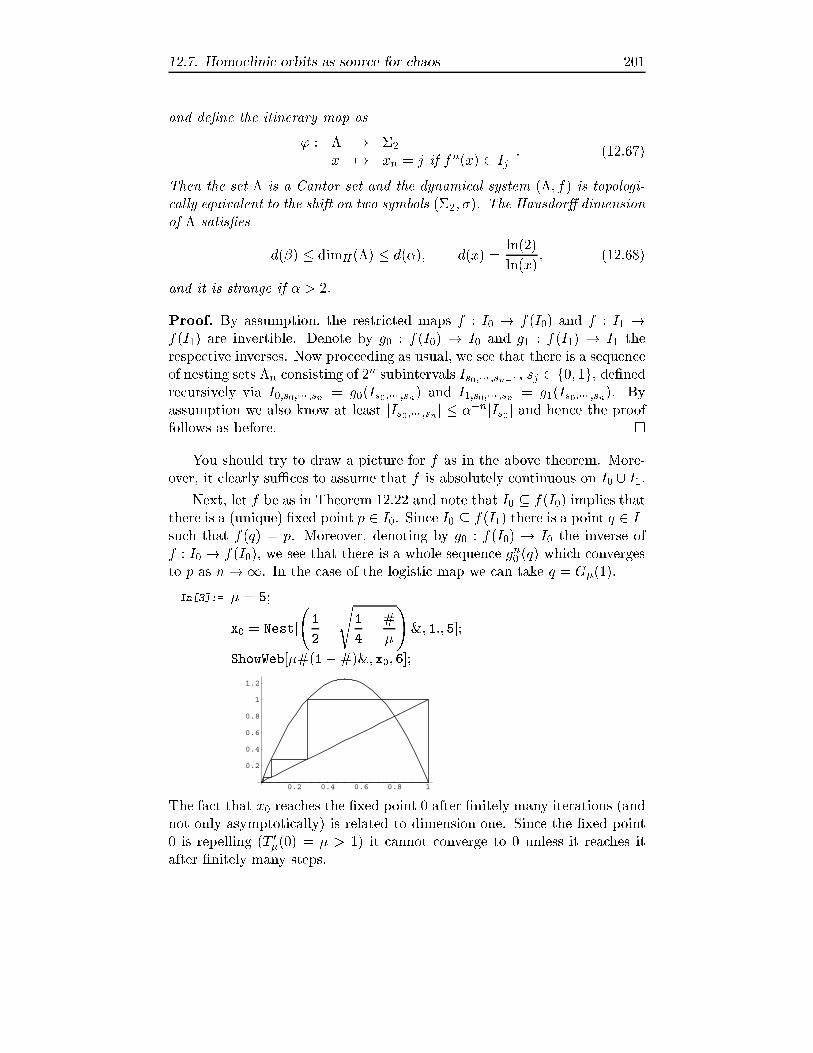
12.7. Homoclinic orbits as source for chaos 201
and de�ne the itinerary map as
' : � ! �2
x 7! xn = j if fn(x) 2 Ij : (12.67)
Then the set � is a Cantor set and the dynamical system (�; f) is topologi-
cally equivalent to the shift on two symbols (�2; �). The Hausdor� dimension
of � satis�es
d(�) � dimH(�) � d(�); d(x) =ln(2)
ln(x); (12.68)
and it is strange if � > 2.
Proof. By assumption, the restricted maps f : I0 ! f(I0) and f : I1 !f(I1) are invertible. Denote by g0 : f(I0) ! I0 and g1 : f(I1) ! I1 the
respective inverses. Now proceeding as usual, we see that there is a sequence
of nesting sets �n consisting of 2n subintervals Is0;��� ;sn�1 , sj 2 f0; 1g, de�ned
recursively via I0;s0;��� ;sn = g0(Is0;��� ;sn) and I1;s0;��� ;sn = g1(Is0;��� ;sn). By
assumption we also know at least jIs0;��� ;sn j � ��njIs0 j and hence the proof
follows as before. �
You should try to draw a picture for f as in the above theorem. More-
over, it clearly suÆces to assume that f is absolutely continuous on I0 [ I1.Next, let f be as in Theorem 12.22 and note that I0 � f(I0) implies that
there is a (unique) �xed point p 2 I0. Since I0 � f(I1) there is a point q 2 I1such that f(q) = p. Moreover, denoting by g0 : f(I0) ! I0 the inverse of
f : I0 ! f(I0), we see that there is a whole sequence gn0 (q) which converges
to p as n!1. In the case of the logistic map we can take q = G�(1).
In[3]:= � = 5;
x0 = Nest[
1
2�s
1
4� #
�
!&; 1:; 5];
ShowWeb[�#(1�#)&; x0; 6];
0.2 0.4 0.6 0.8 1
0.2
0.4
0.6
0.8
1
1.2
The fact that x0 reaches the �xed point 0 after �nitely many iterations (and
not only asymptotically) is related to dimension one. Since the �xed point
0 is repelling (T 0�(0) = � > 1) it cannot converge to 0 unless it reaches it
after �nitely many steps.

202 12. Discrete dynamical systems in one dimension
In general, let f : I ! I be continuously di�erentiable. A �xed point
p is called a hyperbolic repellor if jf 0(p)j > 1. Hence there is a closed
interval W containing p such that jf 0(x)j � � > 1 for all x 2W . Moreover,
by the inverse function theorem there is a local inverse g : f(W )!W such
that g(f(x)) = x, x 2 W . Note that g is a contraction. A point q 2 W is
called a homoclinic point if there exists an n 2 N0 such that f l(q) = p.
The set (q) = ff j(q)jj 2 N0g [ fgj(q)jj 2 Ng is called the corresponding
homoclinic orbit. It is called nondegenerate if (f l)0(q) 6= 0 (which implies
f0(x) 6= 0 for all x 2 (q). A hyperbolic repellor with a homoclinic orbit is
also called a snap back repellor.
Theorem 12.23. Suppose f 2 C1(I; I) has a repelling hyperbolic �xed point
p and a corresponding nondegenerate homoclinic point q.
In every suÆciently small neighborhood U of p there is an n 2 N and an
fn invariant Cantor set � (i.e., fn(�) = �) such that (fn;�) is topologically
equivalent to the shift on two symbols (�2; �).
Proof. We will need to construct two disjoint intervals Ij � U\W , j = 0; 1,
as in Theorem 12.22 for the map F = fn with n suitable. By shrinking W
it is no restriction to assume W � U .
The idea is to take compact intervals I0 containing p and I1 containing
q. Since f l(q) = p, the interval f l(I1) contains again p. Taking suÆciently
many iterations we can blow up both intervals such that the iterated im-
ages contain both original ones. The only tricky part is to ensure that the
derivative of the iterated map is larger than one.
So we start with an interval I1 � W containing q 2 W . Since q is
nondegenerate we can choose I1 such that j(f l)0(x)j � " > 0 for all x 2 I1.
Moreover, by shrinking I1 if necessary we can also assume f l(I1) \ I1 = ;.Next pick m so large that gm(I1) � f
l(I1) (g being the local inverse of f as
above) and �m" > 1. Set n = m + l. Since gm(W ) contains p and gm(I1)
we can further shrink I1 such that f l(I1) � gm(W ), that is, fn(I1) � W .
By construction j(fn)0(x)j � "�m> 1 for x 2 I1.
Next we will choose I0 = gl(f l(I1)). Then we have I0 \ I1 = ; and I0 �
fn(I1) since I0 � f
l(I1). Furthermore, by p 2 I0 we have I0 � fn(I0) and
by gm(I1) � fl(I1) = f
l(I0) we have I1 � fn(I0). Finally, since I0 � g
n(W )
we have j(fn)0(x)j � �n> 1 for x 2 I0 and we are done. �
Why is the degeneracy condition necessary? Can you give a counter
example?
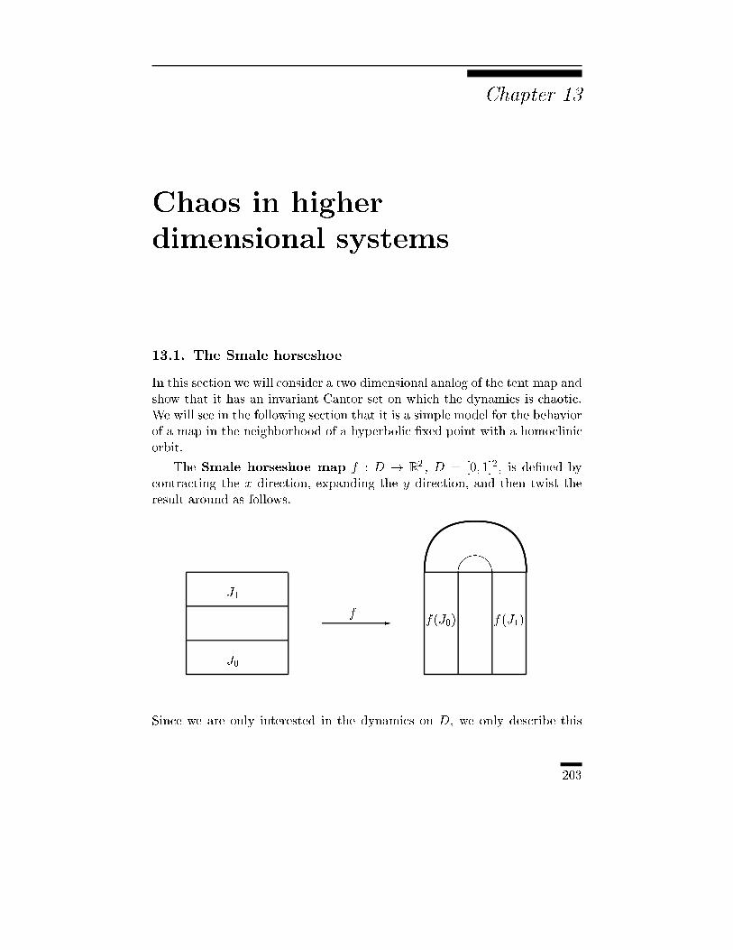
Chapter 13
Chaos in higher
dimensional systems
13.1. The Smale horseshoe
In this section we will consider a two dimensional analog of the tent map and
show that it has an invariant Cantor set on which the dynamics is chaotic.
We will see in the following section that it is a simple model for the behavior
of a map in the neighborhood of a hyperbolic �xed point with a homoclinic
orbit.
The Smale horseshoe map f : D ! R2 , D = [0; 1]2, is de�ned by
contracting the x direction, expanding the y direction, and then twist the
result around as follows.
J0
J1
-f
��
f(J0) f(J1)
Since we are only interested in the dynamics on D, we only describe this
203

204 13. Chaos in higher dimensional systems
part of the map analytically. We �x � 2 (0; 12 ], � 2 [2;1), set
J0 = [0; 1] � [0;1
�]; J1 = [0; 1] � [1� 1
�; 1]; (13.1)
and de�ne
f : J0 ! f(J0); (x; y) 7! (�x; �y); (13.2)
respectively
f : J1 ! f(J1); (x; y) 7! (1� �x; �(1� y)): (13.3)
A look at the two coordinates shows that f1(x; y) 2 [0; 1] whenever x 2 [0; 1]
and that f2(x; y) = T�(y). Hence if we want to stay in D during the �rst
n iterations we need to start in �+;n = [0; 1] � �n(T�), where �n(T�) = �nis the same as for T�. In particular, if we want to stay in D for all positive
iterations we have to start in
�+ = [0; 1] � �(T�) =\n2N0
fn(D): (13.4)
But note that f is invertible, with inverse given by
g = f�1 : K0 = f(J0)! J0; (x; y) 7! (��1x; ��1y); (13.5)
respectively
g = f�1 : K1 = f(J1)! J1; (x; y) 7! (��1(1� x); 1 � �
�1y): (13.6)
Hence, by the same consideration, if we want to stay in D for all negative
iterations, we have to start in
�� = �(T1=�)� [0; 1] =\n2N0
f�n(D): (13.7)
Finally, if we want to stay in D for all (positive and negative) iterations we
have to start in
� = �� \ �+ = �(T1=�)� �(T�): (13.8)
The set � is a Cantor set since any product of two Cantor sets is again a
Cantor set (prove this).
Now by our considerations for the tent map, the y coordinate of every
point in � can uniquely de�ned by a sequence yn, n 2 N0 . Similarly, the
x coordinate of every point in � can be uniquely de�ned by a sequence xn,
n 2 N0 . Hence de�ning sn = yn and s�n = xn�1 for n 2 N0 we see that
there is a one to one correspondence between points in � and doubly in�nite
sequences on two symbols. Hence we have found again an itinerary map
' : � ! �2
(x; y) 7! sn =
�yn n � 0
x�n�1 n < 0
; (13.9)
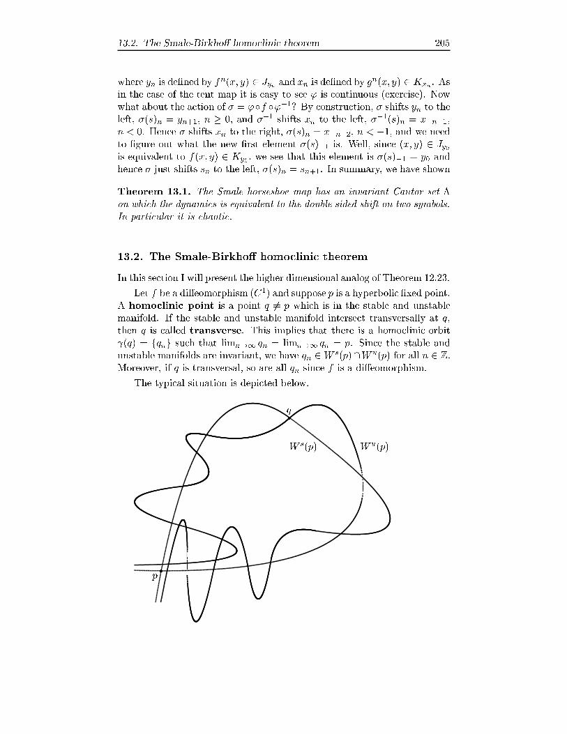
13.2. The Smale-Birkho� homoclinic theorem 205
where yn is de�ned by fn(x; y) 2 Jyn and xn is de�ned by gn(x; y) 2 Kxn . As
in the case of the tent map it is easy to see ' is continuous (exercise). Now
what about the action of � = 'Æf Æ'�1? By construction, � shifts yn to the
left, �(s)n = yn+1, n � 0, and ��1 shifts xn to the left, ��1(s)n = x�n�1,
n < 0. Hence � shifts xn to the right, �(s)n = x�n�2, n < �1, and we need
to �gure out what the new �rst element �(s)�1 is. Well, since (x; y) 2 Jy0
is equivalent to f(x; y) 2 Ky0 , we see that this element is �(s)�1 = y0 and
hence � just shifts sn to the left, �(s)n = sn+1. In summary, we have shown
Theorem 13.1. The Smale horseshoe map has an invariant Cantor set �
on which the dynamics is equivalent to the double sided shift on two symbols.
In particular it is chaotic.
13.2. The Smale-Birkho� homoclinic theorem
In this section I will present the higher dimensional analog of Theorem 12.23.
Let f be a di�eomorphism (C1) and suppose p is a hyperbolic �xed point.
A homoclinic point is a point q 6= p which is in the stable and unstable
manifold. If the stable and unstable manifold intersect transversally at q,
then q is called transverse. This implies that there is a homoclinic orbit
(q) = fqng such that limn!1 qn = limn!1 qn = p. Since the stable and
unstable manifolds are invariant, we have qn 2W s(p)\W u(p) for all n 2 Z.
Moreover, if q is transversal, so are all qn since f is a di�eomorphism.
The typical situation is depicted below.
rp
rq
Ws(p) W
u(p)
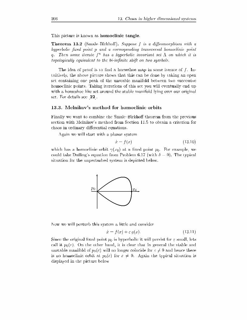
206 13. Chaos in higher dimensional systems
This picture is known as homoclinic tangle.
Theorem 13.2 (Smale{Birkho�). Suppose f is a di�eomorphism with a
hyperbolic �xed point p and a corresponding transversal homoclinic point
q. Then some iterate fn has a hyperbolic invariant set � on which it is
topologically equivalent to the bi-in�nite shift on two symbols.
The idea of proof is to �nd a horseshoe map in some iterate of f . In-
tuitively, the above picture shows that this can be done by taking an open
set containing one peak of the unstable manifold between two successive
homoclinic points. Taking iterations of this set you will eventually end up
with a horseshoe like set around the stable manifold lying over our original
set. For details see [22].
13.3. Melnikov's method for homoclinic orbits
Finally we want to combine the Smale{Birkho� theorem from the previous
section with Melnikov's method from Section 11.5 to obtain a criterion for
chaos in ordinary di�erential equations.
Again we will start with a planar system
_x = f(x) (13.10)
which has a homoclinic orbit (x0) at a �xed point p0. For example, we
could take DuÆng's equation from Problem 6.17 (with Æ = 0). The typical
situation for the unperturbed system is depicted below.
-
6
p0 rx0
Now we will perturb this system a little and consider
_x = f(x) + " g(x): (13.11)
Since the original �xed point p0 is hyperbolic it will persist for " small, lets
call it p0("). On the other hand, it is clear that in general the stable and
unstable manifold of p0(") will no longer coincide for " 6= 0 and hence there
is no homoclinic orbit at p0(") for " 6= 0. Again the typical situation is
displayed in the picture below
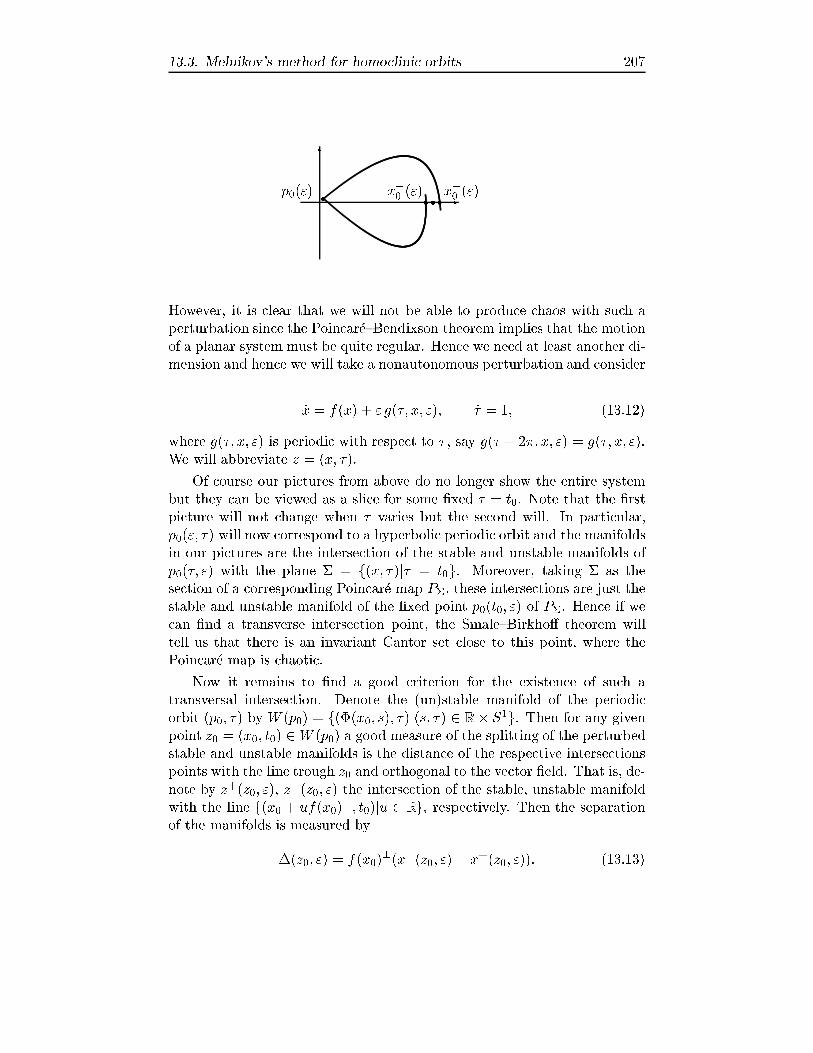
13.3. Melnikov's method for homoclinic orbits 207
-
6
rp0(") rr rx+0 (") x
�0 (")
However, it is clear that we will not be able to produce chaos with such a
perturbation since the Poincar�e{Bendixson theorem implies that the motion
of a planar system must be quite regular. Hence we need at least another di-
mension and hence we will take a nonautonomous perturbation and consider
_x = f(x) + " g(�; x; "); _� = 1; (13.12)
where g(�; x; ") is periodic with respect to � , say g(� + 2�; x; ") = g(�; x; ").
We will abbreviate z = (x; �).
Of course our pictures from above do no longer show the entire system
but they can be viewed as a slice for some �xed � = t0. Note that the �rst
picture will not change when � varies but the second will. In particular,
p0("; �) will now correspond to a hyperbolic periodic orbit and the manifolds
in our pictures are the intersection of the stable and unstable manifolds of
p0(�; ") with the plane � = f(x; �)j� = t0g. Moreover, taking � as the
section of a corresponding Poincar�e map P�, these intersections are just the
stable and unstable manifold of the �xed point p0(t0; ") of P�. Hence if we
can �nd a transverse intersection point, the Smale{Birkho� theorem will
tell us that there is an invariant Cantor set close to this point, where the
Poincar�e map is chaotic.
Now it remains to �nd a good criterion for the existence of such a
transversal intersection. Denote the (un)stable manifold of the periodic
orbit (p0; �) by W (p0) = f(�(x0; s); �)j(s; �) 2 R � S1g. Then for any given
point z0 = (x0; t0) 2W (p0) a good measure of the splitting of the perturbed
stable and unstable manifolds is the distance of the respective intersections
points with the line trough z0 and orthogonal to the vector �eld. That is, de-
note by z+(z0; "), z�(z0; ") the intersection of the stable, unstable manifold
with the line f(x0 + uf(x0)?; t0)ju 2 Rg, respectively. Then the separation
of the manifolds is measured by
�(z0; ") = f(x0)?(x�(z0; ") � x
+(z0; ")): (13.13)

208 13. Chaos in higher dimensional systems
Since �(z0; 0) = 0 we can apply the same analysis as in Section 11.4 to
conclude that �(z0; ") has a zero for small " if@�@" (z0; 0) has a simple zero.
Moreover, if the zero of @�@" (z0; 0) is simple, this is also equivalent to the fact
that the intersection of the stable and unstable manifolds is transversal.
It remains to compute @�@" (z0; 0) which can be done using the same ideas
as in Section 11.4. In fact,
@�
@"(z0; 0) = f(x0)
?(x�" (z0; 0)� x+" (z0; 0)); (13.14)
where x�" (z0; t) are solutions of a corresponding variational equation. How-
ever, since we do not know the initial conditions (we know only the asymp-
totic behavior), it is better to consider
f(x0(t)) ^ x�" (z0; t); x0(t) = �(t; x0): (13.15)
Using the variational equation for x�" (z0; t) we obtain the equation
(A(t)f(x0(t))) ^ x�" (z0; t) + f(x0(t)) _x�" (z0; t)
= f(x0(t)) ^ (A(t)x�" (z0; t)) + f(x0(t)) ^ g(t+ t0; x0(t); 0); (13.16)
where
A(t) = dfx(t): (13.17)
After a little calculation (Problem 13.1) this simpli�es to
f(x0(t)) ^ x�" (z0; t)= tr(A(t))f(x0(t)) ^ x�" (z0; t) + f(x0(t)) ^ g(t+ t0; x0(t); 0) (13.18)
and hence
f(x0(t)) ^ x�" (z0; t) = f(x0(T�)) ^ x�" (z0; T�)
+
Z t
T�
eR tstr(A(r))dr
f(x0(s)) ^ g(s+ t0; x0(s); 0) ds: (13.19)
Next, we want to get rid of the boundary terms at T� by taking the limit
T� ! �1. They will vanish provided x�" (z0; T�) remains bounded since
limt!�1 f(x0(t)) = f(p0) = 0. In fact, this is shown in the next lemma.
Lemma 13.3. The stable and unstable manifolds of the perturbed periodic
orbit p0(") are locally given by
W�( (p0("))) = f(�(s; x0) + h
�(�; s)"+ o("); �)j(s; �) 2 S1 � Rg; (13.20)
where x0 2W (p0) is �xed and h�(�; s) is bounded as s! �1.
Proof. By Theorem 11.10 a point in W�( (p0("))) can locally be written
as
(p0 + h�0 (�; a) + h
�1 (�; a)" + o("); �): (13.21)

13.3. Melnikov's method for homoclinic orbits 209
Moreover, �xing x0 2W (p0) there is a unique s = s(�; a) such that
p0 + h�0 (�; a; 0) = �(s; x0) (13.22)
and hence we can choose h�(�; s) = h�1 (�; a(�; s)). �
Hence we even have
f(x0(t))^x�" (z0; t) =Z t
�1eR tstr(A(r))dr
f(x0(s))^g(s+t0; x0(s); 0) ds (13.23)
and thus �nally
@�
@"(z0; 0) =
Z 1
�1e�
R s0tr(A(r))dr
f(x0(s)) ^ g(s+ t0; x0(s); 0) ds: (13.24)
Since x0 must lie on the homoclinic orbit it is convenient to �x some
point x0 and represent all others by �(t; x0).
Hence, de�ning the homoclinic Melnikov integral
Mx0(t) =
Z 1
�1e�
R s0div(f(�(r;x0)))drf(�(s; x0)) ^ g(s� t;�(s; x0); 0) ds:
(13.25)
we have
@�
@"((�(t; x0); t0); 0) = e�
R t0div(f(�(r;x0)))drMx0(t� t0): (13.26)
In summary we have proven
Theorem 13.4 (Melnikov). Suppose the homoclinic Melnikov integralMx0(t)
has a simple zero for some t 2 R, then the Poincar�e map P� has a transver-
sal homoclinic orbit for suÆciently small " 6= 0.
For example, consider the forced DuÆng equation (compare Problem 6.17)
_q = p; _p = q � q3 � "(Æp + cos(!�)); _� = 1: (13.27)
The homoclinic orbit is given by
q0(t) =p2 sech(t); p0(t) = �
p2 tanh(t)sech(t) (13.28)
and hence
M(t) =
Z 1
�1q0(s) (Æp0(s) + cos(!(s� t))) ds
=4Æ
3�p2� !sech(
�!
2) sin(!t) (13.29)
Thus the DuÆng equation is chaotic for Æ, suÆciently small provided���� Æ ���� < 3
p2�j!j4
sech(�!
2): (13.30)
210 13. Chaos in higher dimensional systems
Problem 13.1. Prove the following formula for x; y 2 R2 and A 2 R
2�R2 ,Ax ^ y + x ^Ay = tr(A)x ^ y:
Problem 13.2. Apply the Melnikov method to the forced mathematical pen-
dulum (compare Section 6.6)
_q = p; _q = � sin(q) + " sin(t):
The End

Bibliography
[1] R. Abraham, J. E. Marsden, and T. Ratiu, Manifolds, Tensor Analysis, and
Applications, 2nd edition, Springer, New York, 1983.
[2] V.I. Arnold, Mathematical methods of classical mechanics, 2nd ed., Springer,New York, 1989.
[3] V.I. Arnold, Gew�ohnliche Di�erentialgleichungen, Springer, Berlin, 1980.
[4] C. Chicone, Ordinary Di�erential Equations with Applications, Springer, NewYork, 1999.
[5] E.A. Coddington and N. Levinson, Theory of Ordinary Di�erential Equations,McGraw-Hill, New York, 1955.
[6] R. Devaney, An introduction to Chaotic Dynamical Systems, Wiley, Chichester ,1995.
[7] K. Falconer, Fractal Geometry, Benjamin/Clummings Publishing, Menlo Park,1986.
[8] A. Gray, M. Mezzino, and M. A. Pinsky, Introduction to Ordinary Di�erential
Equations with Mathematica,
[9] J. Guckenheimer and P. Holmes, Nonlinear Oscillations, Dynamical Systems,
and Bifurcations of Vector Fields, Springer, New York, 1983.
[10] P. Hartman, Ordinary Di�erential Equations, Wiley, New York, 1964.
[11] M. W. Hirsch and S. Smale, Di�erential Equations, Dynamical Systems, and
Linear Algebra, Academic Press, San Diego, 1989.
[12] J. Hofbauer and K. Sigmund, Evolutionary Games and Replicator Dynamics,Cambridge University Press, Cambridge, 1998.
[13] R. A. Holmgren, A First Course in Discrete Dynamical Systems, 2nded.,Springer, New York, 1996.
[14] K. J�anich, Analysis, 2nd ed., Springer, Berlin, 1990.
[15] E.L. Ince, Ordinary Di�erential Equations, Dover Publ., New York, 1956.
[16] E. Kamke, Di�erentialgleichungen, I. Gew�ohnliche Di�erentialgleichungen,Springer, New York, 1997.
211

212 Bibliography
[17] B. M. Levitan and I. S. Sargsjan, Introduction to Spectral Theory, Amer. Math.Soc., Providence, 1975.
[18] J. Moser, Stable and Random Motions in Dynamical Systems: With Special Em-
phasis on Celestial Mechanics, Princeton University Press, Princeton 2001.
[19] R. S. Palais, The symmetries of solitons, Bull. Amer. Math. Soc., 34, 339{403(1997).
[20] J. Palis and W. de Melo, Geometric Theory of Dynamical Systems, Springer,New York, 1982.
[21] L. Perko, Di�erential Equations and Dynamical Systems, 2nd ed., Springer, NewYork, 1996.
[22] C. Robinson, Dynamical Systems: Stability, Symbolic Dynamics, and Chaos,CRC Press, Boca Raton, 1995.
[23] C. A. Rogers, Hausdor� Measures, Cambridge University Press, Cambridge,1970.
[24] D. Ruelle, Elements of Di�erentiable Dynamics and Bifurcation Theory, Aca-demic Press, San Diego, 1988.
[25] D. Schwalbe and S. Wagon, VisualDSolve. Visualizing Di�erential Equations
with Mathematica, Springer, New York, 1997.
[26] C. Sparrow, The Lorenz Equation, Bifurcations, Chaos and Strange Attractors,Springer, New York, 1982.
[27] F. Verhulst, Nonlinear Di�erential Equations and Dynamical Systems, Springer,Berlin, 1990.
[28] W. Walter, Gew�ohnliche Di�erentialgleichungen, Akademische Verlagsge-sellschaft, Leipzig, 1962.
[29] J. Weidmann, Linear Operators in Hilbert Spaces, Springer, New York, 1980.
[30] S. Wiggins, Global Bifurcations and Chaos, 2nd ed., Springer, New York, 1988.
[31] S. Wiggins, Introduction to Applied Nonlinear Dynamical Systems and Chaos,Springer, New York, 1990.
[32] S. Wolfram, The Mathematica Book, 4th ed., Wolfram Media/Cambridge Uni-versity Press, Champaign/Cambridge, 1999.
[33] D. Zwillinger, Handbook of Di�erential Equations, Academic Press, San Diego,1989.

Glossary of notations
A� . . . matrix A restricted to E�(A).
B"(x) . . . ball of radius " centered at x.
C(U; V ) . . . set of continuous functions from U to V .
C(U) = C(U;R)
Ck(U; V ) . . . set of k times continuously di�erentiable functions.
C . . . the set of complex numbers
�A . . . Characteristic polynomial of A, 36
d(U) . . . diameter of U , 196
d(x; y) . . . distance in a metric space
dfx . . . Jacobian of a di�erentiable mapping f at x
E0(A) . . . center subspace of a matrix, 38
E�(A) . . . (un)stable subspace of a matrix, 38
(x) . . . orbit of x, 93
�(x) . . . forward, backward orbit of x, 93
H0 . . . inner product space, 72
Ix = (T�(x); T+(x))
L� . . . logistic map, 158
� . . . a compact invariant set
M� . . . (un)stable manifold, 108, 172
N . . . the set of positive integers
N0 = N [ f0go(:) . . . Landau symbol
O(:) . . . Landau symbol
(f) . . . set of nonwandering points, 97
213
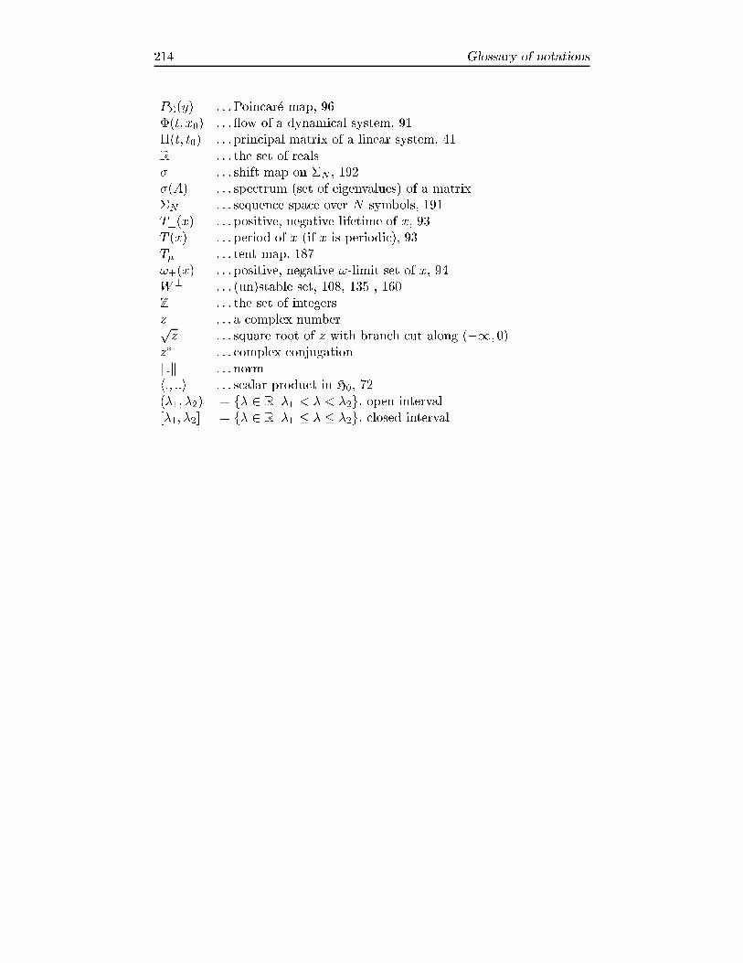
214 Glossary of notations
P�(y) . . . Poincar�e map, 96
�(t; x0) . . . ow of a dynamical system, 91
�(t; t0) . . . principal matrix of a linear system, 41
R . . . the set of reals
� . . . shift map on �N , 192
�(A) . . . spectrum (set of eigenvalues) of a matrix
�N . . . sequence space over N symbols, 191
T�(x) . . . positive, negative lifetime of x, 93
T (x) . . . period of x (if x is periodic), 93
T� . . . tent map, 187
!�(x) . . . positive, negative !-limit set of x, 94
W� . . . (un)stable set, 108, 135 , 160
Z . . . the set of integers
z . . . a complex numberpz . . . square root of z with branch cut along (�1; 0)
z� . . . complex conjugation
k:k . . . norm
h:; ::i . . . scalar product in H0, 72
(�1; �2) = f� 2 R j�1 < � < �2g, open interval
[�1; �2] = f� 2 R j�1 � � � �2g, closed interval

Index
Action integral, 140
Action variable, 146
Angle variable, 146
Angular momentum, 149
Arc, 119
Asymptotic phase, 172
Asymptotic stability, 98, 162, 167
Attracting set, 135
Attractor, 135, 195
strange, 196
Autonomous di�erential equation, 7
Backward asymptotic, 161
Banach space, 17
Basin of attraction, 135
Basis
orthonormal, 73
Bendixson criterion, 123
Bernoulli equation, 13
Bessel
equation, 63
function, 63
inequality, 73
Bifurcation point, 182
Bifurcation theory, 98
Boundary condition, 71
Dirichlet, 77
Neumann, 77
Boundary value problem, 71
Canonical transform, 144
Cantor set, 189
Cauchy sequence, 17
Characteristic exponents, 61
Characteristic polynomial, 36
Commutator, 35
Completely integrable, 146
Con uent hypergeometric equation, 67
Conjugacy
topological, 115
Constant of motion, 100, 142
Contraction principle, 18
Cover, 196
d'Alembert reduction, 44
Diameter, 196
Di�erence equation, 65, 159
Di�erential equation
order, 6
autonomous, 7
exact, 15
homogeneous, 6, 12
integrating factor, 15
linear, 6
ordinary, 5
partial, 7
separable, 10
solution, 6
system, 6
Diophantine condition, 152
Domain of attraction, 135
Dominating function, 32
DuÆng equation, 104, 136, 209
Dulac criterion, 123
Dynamical system, 89
chaotic, 186
continuous, 89
discrete, 89
invertible, 89
Eigenspace, 36
generalized, 36
215
216 Index
Eigenvalue, 36, 74
simple, 74
Eigenvector, 36, 74
Einstein equation, 143
Equilibrium point, see Fixed point
Equivalence
Topological, 186
Euler constant, 65
Euler system, 56
Euler-Lagrange equations, 141
Fermi-Pasta-Ulam experiment, 148
Fibonacci numbers, 164
First integral, 142
First variational equation, 24
periodic, 168
Fixed point, 18, 93, 160
asymptotically stable, 98, 162
hyperbolic, 108
stable, 97
Fixed-point theorem
contraction principle, 18
Weissinger, 19
Flow, 91
Forward asymptotic, 160
Frobenius method, 61
Fuchs system, 62
Gradient systems, 100
Green's formula, 77
Hamilton mechanics, 103, 141
Hamilton principle, 140
Hammerstein integral equation, 117
Hankel function, 65
Harmonic numbers, 64
Harmonic oscillator, 147
Hartman-Grobman theorem, 114
maps, 164
Hausdor� dimension, 197
Hausdor� measure, 196
Heisenberg equation, 45
Hilbert space, 72
Hill equation, 46
Homoclinic orbit, 202
Homoclinic point, 202, 205
transverse, 205
Homoclinic tangle, 206
Hopf bifurcation, 173
Hyperbolic, 106, 108
Hypergeometric equation, 67
Inequality
Gronwall, 22, 24
Initial value problem, 19
Inner product, 72
space, 72
Integral curve, 91
maximal, 91
Integral equation, 19
Hammerstein, 117
Volterra, 33
Itinerary map, 190, 200, 201
Jacobi identity, 148
Jordan block, 37
Jordan canonical form, 38
real, 39
Jordan Curve, 119
Kirchho�'s laws, 128
Kronecker torus, 151
Lagrange function, 140
Laplace transform, 52
Lax equation, 148
Lax pair, 148
Legendre equation, 67
Legendre transform, 141
Leibniz' rule, 148
Li�enard equation, 129
Liapunov function, 99, 162
strict, 99, 162
Lie derivative, 100
Lifetime, 93
Liouville's formula, 42, 139
Lipschitz continuous, 20
Logistic map, 158
Lorenz equation, 136
Manifold
(un)stable, �xed point, 108, 164
(un)stable, linear, 106
(un)stable, periodic point, 172
center, linear, 106
stable, 165
unstable, 165
Mathematical pendulum, 101
Matrix
exponential, 35
norm, 35
Measure
Hausdor�, 196
outer, 196
Melnikov integral
homoclinic, 209
periodic, 175
Monodromy matrix, 45
N-body problem, 150
Nilpotent, 37
Nonresonant, 151
Nonwandering, 97
Norm, 17

Index 217
Normalized, 73
Ohm's law, 128
Omega limit set, 94, 133
Operator
bounded, 74
compact, 74
domain, 74
linear, 74
symmetric, 74
Orbit, 93, 160
asymptotically stable, 167
closed, 93
heteroclinic, 111, 166
homoclinic, 111, 166
periodic, 93
stable, 167
Orthogonal, 73
Parallelogram law, 76
Period anulus, 175
isochronous, 180
regular, 180
Period doubling, 183
Periodic orbit
stable, 162
Periodic point, 93, 160
attracting, 160
hyperbolic, 161
period, 93
repelling, 161
Periodic solution
stability, 167
Phase space, 101
Picard iteration, 21
Pitchfork bifurcation, 98
Pochhammer symbol, 63
Poincar�e map, 96, 168
Point
nonwandering, 97
Poisson bracket, 142
Pr�ufer variables, 81
Quasi-periodic, 152
Reduction of order, 44
Regular point, 93
Relativistic mechanics, 143
Repellor, 195
strange, 196
Resonant, 151
Riccati equation, 13, 44
Riemann equation, 68
Riemann symbol, 68
Runge-Kutta algorithm, 30
Saddle, 106
Saddle-node bifurcation, 98
Sarkovskii ordering, 185
Scalar product, 72
Schr�odinger equation, 44
Schwarz inequality, 73
Sensitive dependence, 185
Separation of variables, 70
Set
attracting, 135, 195
hyperbolic attracting, 196
hyperbolic repelling, 196
invariant, 94
repelling, 195
Shift map, 192
Singular point, see Fixed point
Singularity
regular, 57
simple, 57
Sink, 106
Smale horseshoe, 203
Small divisor, 152
Snap back repellor, 202
Solution
matrix, 41, 42, 163
sub, 13
super, 13
Source, 105
Spectral radius, 41
Spectrum, 36
Stability, 97, 162, 167
Stable set, 108, 135, 160
Stationary point, see Fixed point
Strange attractor, 139
Sturm{Liouville problem, 71
Submanifold, 96
Subshift of �nite type, 193
Subspace
center, 38
invariant, 36
reducing, 36
stable, 38
unstable, 38
Superposition, 41
Symbol space, 191
Symplectic
gradient, 142
group, 144
map, 144
matrix, 141
two form, 144
Tent map, 187
Theorem
Arzel�a-Ascoli, 28, 79
Cayley{Hamilton, 37
Center Manifold, 111
Dominated convergence, 31

218 Index
Floquet, 46
Fuchs, 58
Hartman-Grobman, 114, 164
Jordan Curve, 119
KAM, 152
Liapunov, 100
Melnikov, 209
Noether, 142
Peano, 29
Picard-Lindel�of, 21
Poincar�e's recurrence, 143
Poincar�e{Bendixson, 122
Pythagoras, 73
Smale{Birkho� homoclinic, 206
Stable Manifold, 110, 166, 171
Weissinger, 19
Time-one map, 139
Trajectory, 91
Transcritical bifurcation, 98
Transformation
�ber preserving, 11
Transition matrix, 193
irreducible, 194
Transitive, 135, 185
Trapping region, 135
Two body problem, 149
Uniform contraction principle, 30
Unstable set, 108, 135, 161
Van der Pol equation, 131
Variable
dependent, 6
independent, 6
Variation of constants, 43
Vector �eld, 90
complete, 94
Vector space, 17
complete, 17
normed, 17
Volterra integral equation, 33
Volterra{Lotka equations, 123
Wave equation, 69
Well-posed, 22
Wronski determinant, 42
Wronskian
modi�ed, 77
Copyright © 2022 FDOKUMEN