arX

iv:1

208.

5147

v2 [

cond

-mat

.sta

t-m

ech]

29

Apr

201

3

Coarse grained approach for volume conserving models

D. Hansmann∗1 and R. C. Buceta†1,2

1Departamento de Fısica, FCEyN, Universidad Nacional de Mar del Plata2Instituto de Investigaciones Fısicas de Mar del Plata, UNMdP and CONICET

Funes 3350, B7602AYL Mar del Plata, Argentina

April 30, 2013

Abstract

Volume conserving surface (VCS) models without deposition and evaporation, as well as ideal molecular-beam epitaxy models, are prototypes to study the symmetries of conserved dynamics. In this work westudy two similar VCS models with conserved noise, which differ from each other by the axial symmetryof their dynamic hopping rules. We use a coarse-grained approach to analyze the models and show howto determine the coefficients of their corresponding continuous stochastic differential equation (SDE) withinthe same universality class. The employed method makes use of small translations in a test space whichcontains the stationary probability density function (SPDF). In case of the symmetric model we calculate allthe coarse-grained coefficients of the related conserved Kardar-Parisi-Zhang (KPZ) equation. With respectto the symmetric model, the asymmetric model adds new terms which have to be analyzed, first of all thediffusion term, whose coarse-grained coefficient can be determined by the same method. In contrast to othermethods, the used formalism allows to calculate all coefficients of the SDE theoretically and within limitsnumerically. Above all, the used approach connects the coefficients of the SDE with the SPDF and hencegives them a precise physical meaning.

1 Introduction

The roughening properties of nonequilibrium surface systems with well-defined power-law behavior can beclassified into universality classes by a unique set of exponents, which determine their dynamical scaling [1].Discrete models and continuous equations within the same universality class share the same scaling exponents,which can be shown by numerical and analytical methods. In order to determine these exponents, manydiscrete models and continuous stochastic differential equations (SDE) have been studied using simulations,symmetry analyses, dynamical renormalization group theory, or numerical integration [2].

Discrete models and continuous SDE within the same universality class share not only the same scalingexponents, but also the same linearities and (or) nonlinearities [3]. In this context, models belonging theKardar-Parisi-Zhang (KPZ) [4] or to the conserved KPZ universality class are of special importance, sincefor these models it is possible to determine the nonlinearities via Monte Carlo simulations using the interfacetilting method [5,6]. Another method, which is not limited to the calculation of the KPZ-nonlinearities, wasintroduced by Vvedensky et al. [7]. They start this calculation from a discrete SDE (or discrete Langevinequation) and determine the continuous counterpart of the discrete SDE using an analytical approach. Theapproach is based on the regularization of the Heaviside Θ-function and on the coarse grain approximationusing a lattice constant which tends to zero [8–11]. The standard procedure to regularize a function is toreplace each Heaviside Θ-function by a smooth function θε, which is continuously differentiable to any orderand depends on a regularization parameter which has to be chosen in a way that θε → Θ when ε → 0.For details, see Appendix A. The regularization function θε has to be analytic throughout its domain, butespecially at zero, in order to enable a Taylor series expansion. The Taylor coefficients depend on both,the regularization prescription (i.e. the regularization function chosen) and the regularization parameter

∗David.Hansmann@gmx.net†rbuceta@mdp.edu.ar

1

ε. As pointed out by Katzav and Schwartz [12] this expansion is problematic since in the limit ε → 0 theHeaviside Θ-function is not analytic around zero. Consequently the parameter cannot be removed in theprocess of coarse-graining. Another weak point of the method is the difficulty of reaching conclusive resultsin models of higher dimensions than one. Finally, although the mathematical derivation is direct, it cangenerate discrepancies in interpretation of coarse coefficients of the continuous differential equation.

Recently, we introduced a different coarse-grained approach based on generalized function or distributiontheory [13]. We showed, that using our approach, it is possible to calculate not only nonlinear, but also, allcoefficients of the stochastic differential equation for a given discrete model of the KPZ universality class.In this work we use our formalism to show, how to determine the coarse-grained coefficients of two volumeconserving surface models.

There are two well-defined groups of models and equations as distinguished by their noise, which is eithernon-conservative or conservative. Growth models and equations which describe deposition or evaporationprocess are included in the first group. In contrast, volume conserving surface (VCS) models withoutdeposition or evaporation are included in second group. The models studied in this work are VCS modelsand consequently have conservative noise. Volume conserving processes are defined as physical processeswhich occur on the surface of a solid and preserve the total volume enclosed by the surface. These processesdescribe the movement of a particle from a site of the surface to another, and exclude particle depositionor evaporation. The conserved noise is assumed to be Gaussian distributed and uncorrelated. It has anexpectation value of zero and the correlation is

〈η(~x, t) η(~x′, t′)〉 = −2Q∇2δ(~x − ~x′) δ(t− t′) , (1)

with ~x ∈ Rd and where the conserved noise intensity Q is proportional to the temperature of the system.

The conserved KPZ (cKPZ) equation [h = h(~x, t), ν < 0, and λ < 0]

∂h

∂t= ∇2

[

ν∇2h+λ

2

(

∇h)2]

+ η(~x, t) , (2)

proposed by Sun et al. [14] describes the first continuous VCS process with conserved noise. The expressionin the brackets of eq.(2) we call KPZ kernel of the equation. In the first molecular-beam epitaxy (MBE)models, eq. (2) reappears with an additive constant F that takes the deposition flux into account. Thisextended equation is called Villain-Lai-Das Sarma (VLD) equation, named by the authors of the article itwas first time mentioned [3, 15]. In contrast to the noise term of the cKPZ equation, the noise term ofthe VLD equation describes non-conservative noise. It has an expectation value of zero and the correlation〈η(~x, t) η(~x′, t′)〉 = −2Dδ(~x−~x′) δ(t−t′), where the noise intensity D is proportional to the flux F . Althoughthe cKPZ and VLD equations have the same KPZ kernel, the equations show distinct macroscopic properties,which have been identified and studied in various scientific works [16]. Since both equations have the samekernel, these distinct properties can be attributed the different nature of their noise.

A VCS model can be described by the continuity differential equation or conservation law

∂h

∂t+∇ · j = η , (3)

where j = j(~x, t) is the surface diffusion current and η = η(~x, t) is the conserved noise. The form of thecurrent j is determined by the symmetries of the system. The current cannot depend explicitly on h, sincethis would break the invariance under constant height translations. It is expected that under nonequilibriumconditions the total current j has two terms, i.e. j = −∇µne + jne. Here µne is the nonequilibrium chemicalpotential and jne is the nonequilibrium current. From symmetry consideration it is expected that µne is afunction of ∇2h and ∇h.

The first model studied in this work has both of these terms. Its dynamic rules are axial symmetric,which means, that a randomly chosen particle hops independently from the actual surface configuration withthe same probability to left as it hops to the right. Its KPZ kernel [see the eq. (2)] is proportional to µne.Furthermore it is expected that jne is an odd function of ∇h.

The second model studied in this work has both types of current contribution, ∇µne and jne. Its dynamicrules are not axial symmetric, which means, that it depends on the surface configuration whether a randomlychosen particle hops to the left or to the right. In order to study their models, the majority of theoreticalstudies employ expansions of j in powers of∇h, its derivatives, and their combinations taking into account thesymmetries of the system. The most relevant term of these expansions is determined by the long wavelengthlimit after renormalization [17].

2

The main goal of this work is to introduce an approach that allows to determine the coarse-grainedcoefficients of the continuous SDE. Additionally, we show how to use the approach to calculate coarse-grained coefficients related to two different discrete VCS models, one with symmetric hopping rules and theother with asymmetric hopping rules. The paper is organized as follows. In Section 2 we developed somebasic concepts and the theoretical formalism which is used to study the chosen models. In this context wegive an overview on the conserved dynamics and conserved noise. In Section 3 we introduce a theoreticalapproach that allows to determine the coarse-grained coefficients using generalized functions or distributionstheory and proper test functions. We show how to obtain these distributions and the test functions. Wediscuss how small changes of the test functions together with a Taylor expansion of the distribution can beused to calculate the coarse-grained observables by applying the expanded distributions to test functions.In Sections 4 and 5 we applying the formalism on the chosen discrete VCS models. We obtain analyticalexpressions for the coefficients in terms of test functions. In Appendix A we show how to calculate thecoarse-grained coefficients using the standard coarse-grained approach via the regularization of Θ-functions.In Appendix B we evaluate the results of Section 4 and 5 numerically using Monte Carlo simulations. Section 6finishes the paper with our conclusions.

2 Volume conserving models

By definition, volume conserving surface models keep the total number of particles enclosed by the surfaceconstant. The movement of the particles can only increase (or decrease) the height of a surface site at theexpense of decreasing (or increasing) the height of another surface site. Thus, the average velocity of thesurface growth is zero and expectation value of the surface height is constant. We assume a discrete processthat takes place on a square lattice with unit cell of side a. Further it is assumed, that a randomly chosenparticle can move only one unit in a unit time. The surface configuration H of the system is determinedby set of heights {hj} which correspond to the columns j = 1, . . . , N . The heights hj of the columns j aremultiples of the unit cell size a, i.e. hj = nja such that nj ∈ Z.

The transition rate W (H ,H ′) of a VCS model, which describes the change between two consecutivesurface configurations H and H ′ in the lapse τ , is

W (H,H ′) =1

τ

N∑

k=1

[ω+k ∆(h′

k, hk − a)∆(h′k+1, hk+1 + a)

+ω−k+1 ∆(h′

k+1, hk+1 − a)∆(h′k, hk + a)]

∏

j 6=k,k+1

∆(h′j , hj) , (4)

where ω+k and ω−

k+1 are the hopping rates from column k to column k+1, and from column k+1 to columnk, respectively. Here ∆(x, y) is equal to 1 if x = y and equal to 0 in all other cases. The hopping rates dependon the height differences between the chosen column and its nearest-neighbor (NN) columns. Explicitly, ω±

j

is function of hj+1 − hj and hj−1 − hj . The first transition moment is

K(1)j =

∑

H′

(h′j − hj)W (H ,H ′) =

a

τ(ω−

j+1 − ω−j − ω+

j + ω+j−1) , (5)

and the second transition moment, written in an equivalent form to the expression used by ref. [18, eq. 6], is

K(2)ij =

∑

H′

(h′i − hi)(h

′j − hj)W (H,H ′)

= −a2

2τ

[

(

ω+i + ω−

i + ω+i−1 + ω−

i+1

)(

δi+1,j − 2 δi,j + δi−1,j

)

+(

ω+i − ω−

i − ω+i−1 + ω−

i+1

)(

δi+1,j − δi−1,j

)

]

, (6)

where δi,j is the Kronecker delta. Note that the first term in brackets contains the symmetric contributionsand the second term in brackets contains the asymmetric contributions. If the hopping rates away from achosen column i are equal, i.e. ω+

i = ω−i , and the hopping rates towards the column i are also equal i.e.

ω+i−1 = ω−

i+1, then eq. (4) has only symmetric contributions. This means, that in this case the jumping ratesand the second transition moment are invariant to the exchange of hi−n↔ hi+n (with n = 1, 2) around tocolumn i.

3

Starting from the Master equation of the transition probability given by eq. (4) and performing a Kramers-Moyal expansion [19–21], it is possible to derive an associated discrete Langevin equation

dhj

dt= K

(1)j + ηj(t) , (7)

with j = 1, . . . , N . The expectation value of the noise ηj is zero and the correlation is

〈ηi(t)ηj(t′)〉 = K

(2)ij δ(t− t′) . (8)

Jung and Kim showed [18] that the continuous SDE can be achieved from its discrete counterpart [eq. (7)]following the approach introduced by Vvedensky et al. [7]. In Appendix A we use this approach to calculatethe coarse-grained coefficients of the models which we discuss in the Sections (4) and (5) in terms of theregularizing coefficients.

3 A bridge from discrete to continuous processes of the sameuniversality class

According to the previous section, the particle hopping rate ω±j from the column j → j ± 1 is a function

of the integer set {σj± = (hj±1 − hj)/a}. Thus, the transition moments K(1)j and K

(2)ij [eqs. (5) and (6),

respectively] depend on the hopping rates and the hopping rates are functions of the height differencesbetween the NN columns and the selected column. The identity ω+

j = ω−j is a fundamental property of the

studied system which is indispensable to extract all the coarse-grained properties derived from the transitionmoments. Using the transition rates ω±

j we define a generalized function W() with ∈ R2. We assume,

that this generalized function matches with the hopping rates, i.e. W( = σj) = ω±j with σj ∈ Z

2. Thegeneralized function W can be decomposed in a symmetric Ws and an antisymmetric Wa term in order tocalculate coarse-grained observables.

In order to calculate the statistical observables of discrete processes it is necessary to define test functionsϕ on which the generalized functions of can be applied. These test functions ϕ have to have differentproperties for restricted and unrestricted processes. Restricted processes require that ϕ ∈ D(R2

ε), where D isthe test space of C∞-functions with compact support andR2

ε = ε−neighborhood(R2). Unrestricted processesrequire that ϕ ∈ S(R2), where S is the test space of C∞-functions that decay and have derivatives of all ordersthat vanish faster than any power of −1

α (α = 1, 2). In the present work we define the test functions on thebase of the surface configuration. For each column j we have two random integer variables that define a surfaceconfiguration vector σj = (σj−, σj+) ∈ Z

2. The chance to find a column j with the surface configurationσj at the time t is given by the time dependent probability density function P (σj , t). One can show viaMonte Carlo simulations, that the time dependent probability density function converges rather fast. Hence,for t ≫ 1 one can interpret P (σj , t) as a time independent, stationary probability density function Pst(σj)(SPDF). The set of surface configurations in the steady state is Z2 = {σj ∈ Z

2/Pst(σj) 6= 0, ∀j = 1, . . . , N} .In the present work the steady state configuration space Z2 is a 2-dimensional lattice within a compact setR2 ⊂ (R2\Z2)∪Z2. We define the test function ϕ() as a real-valued function, that matches with the discreteSPDF, i.e. ϕ( = σj) = Pst(σj) with σj ∈ Z

2. Fig. 1 shows the test functions of both the unrestricted VCSmodels considered in this work.

The application of a distribution f ∈ D′ (dual space of D) to test function ϕ ∈ D is defined by

〈f , ϕ〉 =

∫

R2

f()ϕ() dv . (9)

We used here the notation on distributions that was introduced by Schwartz [22]. Note that 〈f, ϕ〉 is the“expectation” value of f using the test function ϕ as real-valued analytic “representation” of the SPDF Pst.Thus, the test function is normed, i.e. 〈1, ϕ〉 = 1 . The translation Tα of a distribution f , denoted Tαf orsimply fα, extends the definition given by eq. (9)

〈Tαf , ϕ〉 = 〈f , T−α ϕ〉 , (10)

where the translation operator is defined by Tx : y 7→ y − x if y ,x ∈ R2 [23]. As mentioned above, we

assume that the test function ϕ takes fixed values in the discrete lattice Z2 given by the SPDF Pst, i.e.〈δσ , ϕ〉 = ϕ(σ) = Pst(σ) for all σ ∈ Z2 , where δσ = Tσδ and δ is the Dirac distribution.

4

Applying a translation Tu to a point ∈ supp(ϕ), the test function transforms as ϕ → Tuϕ if (−u) ∈supp(ϕ). Furthermore w = 〈W , ϕ〉, the expectation value of W , changes as w(0) → w(u) with

w(u) = 〈W , Tuϕ〉 =

∫

R2

W() ϕ(− u) dv . (11)

For small translations, the Taylor expansion of ϕ(− u) around u = 0 is

ϕ(− u) = ϕ()− uα ∂αϕ⌋

u=0+ 1

2 uαuβ ∂2αβϕ

⌋

u=0+O(3) . (12)

Here repeated subscripts imply sums, uα is the α-th component of u, ∂α = ∂/∂α, and ∂2αβ = ∂2/(∂α∂β),

with α , β = 1, 2. Since the test function ϕ is known only at points of the lattice Z2, its derivatives can notbe calculated explicitly. In contrast, the distribution W is derivable in all points. Since the test function haseither compact support or decreases rapidly one can take advantage of the following identity

⟨

W , ∂nαβ···ωϕ

⟩

= (−1)n⟨

∂nαβ···ωW , ϕ

⟩

. (13)

Using eqs. (11–13), the observable is transformed according to

w(u) =⟨

W , ϕ⟩

+⟨

∂αW , ϕ⟩

uα + 12

⟨

∂2αβW , ϕ

⟩

uαuβ +O(3) . (14)

In a previous work [13] we used the mentioned translations to determine the coarse-grained coefficientsfor a restricted and an unrestricted discrete KPZ-type model: the restricted solid-on-solid model and theballistic deposition model, respectively. We derive their coefficients from the transformed average velocityof the interface v(u) = 〈K(1), Tuϕ〉 where the first transition moment K(1) is the drift of correspondingLangevin equation. The VCS models studied in the following sections have no restrictions, although thetheory allows the treatment of models with restrictions, as shown in previous studies. In contrast to thisformer work, the presently studied models allow to calculate analytically another observable quantity whichis the non-conserved noise intensity. This is possible by intervening in the equivalent continuous process, inthis case via the application of small changes to D = 〈K(2), ϕ〉, where K(2) is the second transition momentcorresponding to discrete process and D is the noise intensity corresponding to equivalent continuous process.

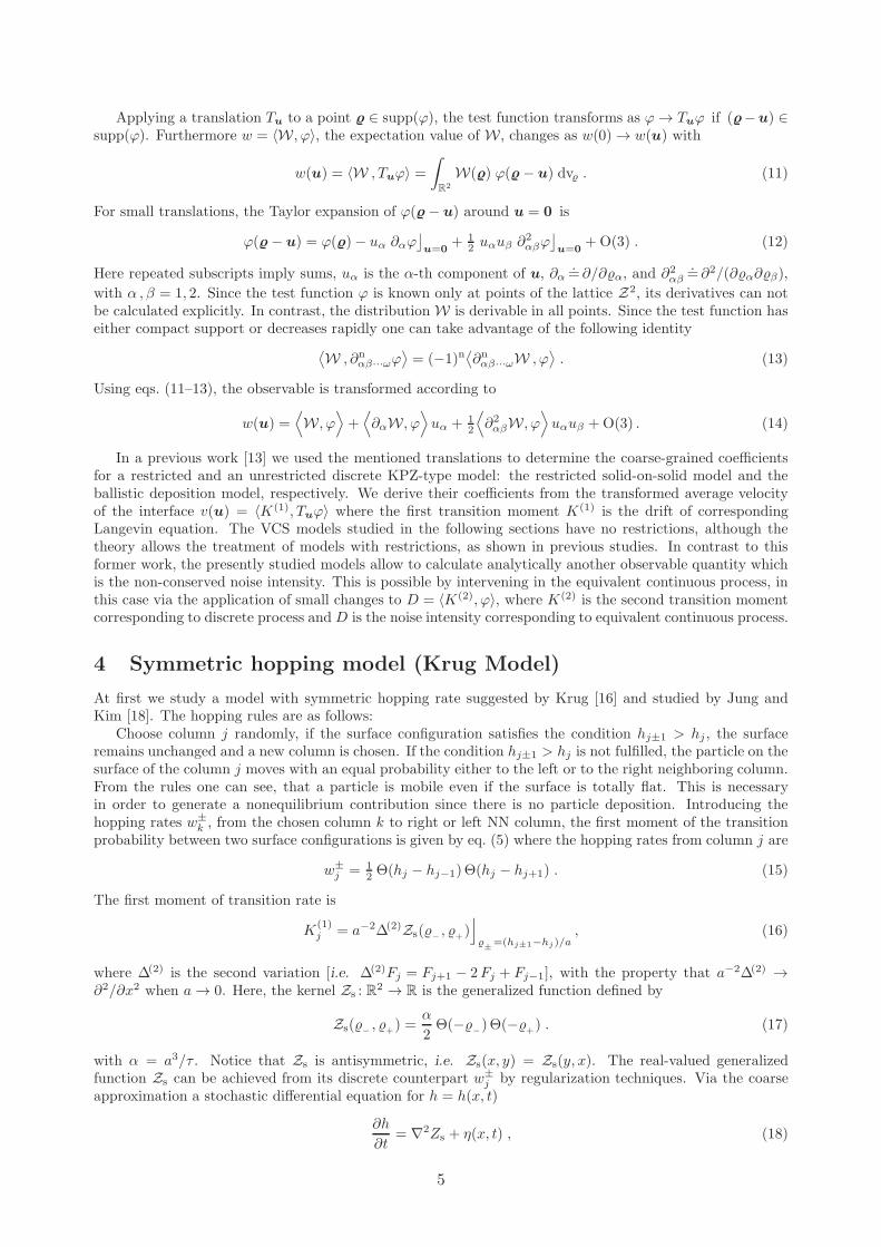
4 Symmetric hopping model (Krug Model)

At first we study a model with symmetric hopping rate suggested by Krug [16] and studied by Jung andKim [18]. The hopping rules are as follows:

Choose column j randomly, if the surface configuration satisfies the condition hj±1 > hj , the surfaceremains unchanged and a new column is chosen. If the condition hj±1 > hj is not fulfilled, the particle on thesurface of the column j moves with an equal probability either to the left or to the right neighboring column.From the rules one can see, that a particle is mobile even if the surface is totally flat. This is necessaryin order to generate a nonequilibrium contribution since there is no particle deposition. Introducing thehopping rates w±

k , from the chosen column k to right or left NN column, the first moment of the transitionprobability between two surface configurations is given by eq. (5) where the hopping rates from column j are

w±j = 1

2 Θ(hj − hj−1)Θ(hj − hj+1) . (15)

The first moment of transition rate is

K(1)j = a−2∆(2)Zs(−

, +)⌋

±=(hj±1−hj)/a

, (16)

where ∆(2) is the second variation [i.e. ∆(2)Fj = Fj+1 − 2Fj + Fj−1], with the property that a−2∆(2) →∂2/∂x2 when a → 0. Here, the kernel Zs : R

2 → R is the generalized function defined by

Zs(−,

+) =

α

2Θ(−

−)Θ(−

+) . (17)

with α = a3/τ . Notice that Zs is antisymmetric, i.e. Zs(x, y) = Zs(y, x). The real-valued generalizedfunction Zs can be achieved from its discrete counterpart w±

j by regularization techniques. Via the coarseapproximation a stochastic differential equation for h = h(x, t)

∂h

∂t= ∇2Zs + η(x, t) , (18)

5

can be obtained, where the KPZ kernel is

Zs = ν∇2h+λ

2|∇h|2 . (19)

Here and below, we use the following notation for the partial derivative ∇.= ∂/∂x. Equation 18 is a

conserved Kardar-Parisi-Zhang equation with conservative noise [14] whose expectation value is zero andwith the correlation function given by eq. (1). In the Appendix A we find this equation using coarse-grainedtechniques via regularization by an alternative way to reference [18]. The coefficients ν and λ of KPZ kernelin terms of the regularizing constants are given in eqs. (39) and (40), respectively.

Instead of using coarse-grained techniques via regularization, the coefficients ν and λ can be obtained byapplying the distribution Zs [eq. (17)] on translated test functions Tuϕ. We introduce the transformations

±→

±+u

±and we assume that gradient and Laplacian transform with u

−1−u

+1= 2 s and u

−1+u

+1=

2 r , respectively. Considering a translation u = (r + s, r − s) and taking into account that ϕ is symmetricunder exchange

−↔

+one calculates

zs(r, s) =⟨

Zs , Tuϕ⟩

= ω0 + ν r + 12 λ s

2 +O(r2, s3) , (20)

where

ω0 = 〈Zs, ϕ〉 ,

ν = 2 〈∂ℓZs , ϕ〉 , (21)

λ = 2 〈(∂2ℓℓ − ∂2

ℓk)Zs , ϕ〉 ,

with ℓ = k = ±1 and ℓ 6= k, where repeated subscripts do not imply sums. Here ϕ(x, y) is the (symmetric)test function. For discrete values x, y ∈ Z the test function ϕ(x, y) takes the same value as the probabilitydensity function Pst(x, y). Taking in to account that

∂ℓZs = − 12 α δ(ℓ)Θ(−k) ,

∂2ℓkZs = 1

2 α δ(ℓ) δ(k) ,

∂2ℓℓZs = − 1

2 α δ′(ℓ)Θ(−k) ,

we obtain

ω0 =α

2

∫ ∫ 0

−∞

ϕ(x, y) dxdy , (22)

ν = −α

∫ 0

−∞

ϕ(0, y) dy , (23)

λ = −α

[

ϕ(0, 0)−

∫ 0

−∞

∂xϕ⌋

(0,y)dy

]

. (24)

We can easily show that the noise intensity of correlation function [eq. (1)] is Q = a2 zs(u) = a2 ω0 + O(1)for all translation u with |u| ≪ 1. When a → 0 the noise intensity is

Q = a2 ω0 . (25)

Please note, that using our approach we have obtained the three coarse-grained coefficients which characterizethe conserved KPZ equation. The algebraic signs of these results are in agreement with the algebraic signsobtained using the coarse-grained approach via regularization [18].

5 Asymmetric hopping model

In this section we study a model with asymmetric hopping rate introduced by Jung and Kim [18]. Incontrast to the previous studied model where a chosen particle moves, independently from the local surfaceconfiguration with the same probability to the left or to the right side, here a chosen particle moves to theNN column which has the lower height. If the heights of the NN columns are both lower than the height ofthe selected column, the particle hops randomly to one of them. Thus the symmetry of the Krug model isbroken. The hopping rates for this model are

ω±k = 1

2 Θ(hk − hk−1)Θ(hk − hk+1)[

1− sgn(hk±1 − hk∓1)]

, (26)

6

Figure 1: The figure shows the test space. Left: symmetric hopping model. Right: asymmetric hoppingmodel. In the test space one sees a test function ϕ(+,−) (semi-transparent) and the discrete probabilitydensity function Pst(σ+, σ−) (black bullets). One sees, that the test function matches with the discreteprobability density function for = σ. The test function ϕ is smooth though not visually fit.

where sgn(z) = Θ(z) − Θ(−z) is the sign function. The first and second term are the symmetric andantisymmetric contributions to hopping rate ω±

j under the exchange hj−1 ↔ hj+1 respectively. In contrast

to the hopping rate ω±j , the hopping rate ω±

j∓1 is asymmetric under the exchange hj−n ↔ hj+n (n = 1, 2).The first moment of the transition rate is

K(1)j =

[ 1

a2∆(2)Zs(−

, +) +

1

2a∆(1)2 Za(−

, +)]

⌋

±=(hj±1−hj)/a

, (27)

where Zs is the symmetric contribution known from the Krug model given by eq. (17) and ∆(1)2 is the first

variation between the NN columns [i.e. ∆(1)2 Fj = Fj+1 − Fj−1] with the property (2 a)−1∆

(1)2 → ∂/∂x when

a → 0. Just like in the case of the Krug model, the kernel Za : R2 → R is interpreted as a generalized

function defined byZa(−

, +) = −βΘ(−

+)Θ(−

−) sgn(

+−

−) . (28)

with β = a2/τ . Notice that Za is antisymmetric, i.e. Za(x, y) = −Za(y, x).By regularization techniques and the coarse approximation a stochastic differential equation can be

obtained. In this case [h = h(x, t)] is

∂h

∂t= ∇2Zs +∇ · Za + η(x, t) , (29)

where the antisymmetric kernel isZa = ν0 ∇h+ γ∇h |∇h|2 , (30)

and Zs is the KPZ kernel eq. (19) with coefficients given by eqs. (22)–(24).We perform a translation u = (s,−s) on the surface configuration space with s ≪ 1, taking into account

that ϕ is symmetric in its variables

za(s) = 〈Za , Tuϕ〉 = ν0 s+ γ s3 +O(5) , (31)

where za(s) = and

ν0 =⟨

(∂x − ∂y)Za , ϕ⟩

,

γ =⟨

(∂x − ∂y)(3)Za , ϕ

⟩

. (32)

Eq. (31) contains only odd powers in s since Za is antisymmetric and contributes only to their odd orderderivatives which are symmetrical. Below we show only the first term, although the calculations can beextended to higher order. Taking into account that

(∂x − ∂y)Za(x, y) =[

δ(x)Θ(−y)− δ(y)Θ(−x)]

sgn(x− y)− 4Θ(−x)Θ(−y) δ(x− y) ,

we obtain

ν0 = 2 β

∫ 0

−∞

[

ϕ(0, x) − 2ϕ(x, x)]

dx . (33)

7

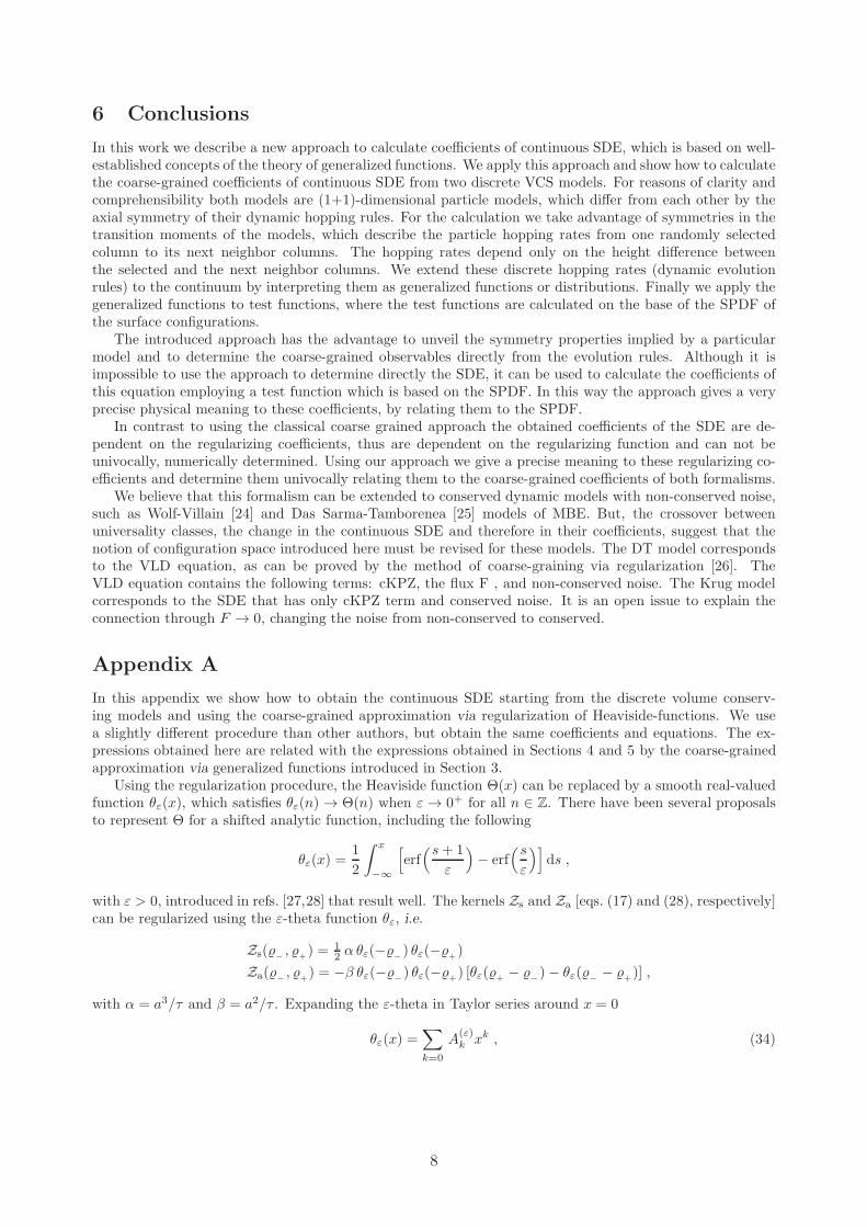
6 Conclusions

In this work we describe a new approach to calculate coefficients of continuous SDE, which is based on well-established concepts of the theory of generalized functions. We apply this approach and show how to calculatethe coarse-grained coefficients of continuous SDE from two discrete VCS models. For reasons of clarity andcomprehensibility both models are (1+1)-dimensional particle models, which differ from each other by theaxial symmetry of their dynamic hopping rules. For the calculation we take advantage of symmetries in thetransition moments of the models, which describe the particle hopping rates from one randomly selectedcolumn to its next neighbor columns. The hopping rates depend only on the height difference betweenthe selected and the next neighbor columns. We extend these discrete hopping rates (dynamic evolutionrules) to the continuum by interpreting them as generalized functions or distributions. Finally we apply thegeneralized functions to test functions, where the test functions are calculated on the base of the SPDF ofthe surface configurations.

The introduced approach has the advantage to unveil the symmetry properties implied by a particularmodel and to determine the coarse-grained observables directly from the evolution rules. Although it isimpossible to use the approach to determine directly the SDE, it can be used to calculate the coefficients ofthis equation employing a test function which is based on the SPDF. In this way the approach gives a veryprecise physical meaning to these coefficients, by relating them to the SPDF.

In contrast to using the classical coarse grained approach the obtained coefficients of the SDE are de-pendent on the regularizing coefficients, thus are dependent on the regularizing function and can not beunivocally, numerically determined. Using our approach we give a precise meaning to these regularizing co-efficients and determine them univocally relating them to the coarse-grained coefficients of both formalisms.

We believe that this formalism can be extended to conserved dynamic models with non-conserved noise,such as Wolf-Villain [24] and Das Sarma-Tamborenea [25] models of MBE. But, the crossover betweenuniversality classes, the change in the continuous SDE and therefore in their coefficients, suggest that thenotion of configuration space introduced here must be revised for these models. The DT model correspondsto the VLD equation, as can be proved by the method of coarse-graining via regularization [26]. TheVLD equation contains the following terms: cKPZ, the flux F , and non-conserved noise. The Krug modelcorresponds to the SDE that has only cKPZ term and conserved noise. It is an open issue to explain theconnection through F → 0, changing the noise from non-conserved to conserved.

Appendix A

In this appendix we show how to obtain the continuous SDE starting from the discrete volume conserv-ing models and using the coarse-grained approximation via regularization of Heaviside-functions. We usea slightly different procedure than other authors, but obtain the same coefficients and equations. The ex-pressions obtained here are related with the expressions obtained in Sections 4 and 5 by the coarse-grainedapproximation via generalized functions introduced in Section 3.

Using the regularization procedure, the Heaviside function Θ(x) can be replaced by a smooth real-valuedfunction θε(x), which satisfies θε(n) → Θ(n) when ε → 0+ for all n ∈ Z. There have been several proposalsto represent Θ for a shifted analytic function, including the following

θε(x) =1

2

∫ x

−∞

[

erf(s+ 1

ε

)

− erf(s

ε

)]

ds ,

with ε > 0, introduced in refs. [27,28] that result well. The kernels Zs and Za [eqs. (17) and (28), respectively]can be regularized using the ε-theta function θε, i.e.

Zs(−,

+) = 1

2 α θε(−−) θε(−

+)

Za(−,

+) = −β θε(−

−) θε(−

+) [θε(+

− −)− θε(−

− +)] ,

with α = a3/τ and β = a2/τ . Expanding the ε-theta in Taylor series around x = 0

θε(x) =∑

k=0

A(ε)k xk , (34)

8

gives the following expansions (superscripts are omitted hereafter)

Zs(−,

+) =

1

2α

[

A20 −A0A1

(

−+

+

)

+(2A0A2 −A2

1)

2(γ + 1)

(

2−− 2γ

−

++ 2

+

)

+O(3)

]

(35)

Za(−,

+) = −β

[

2A20A1

(

+−

−

)

+O(3)]

,

where

γ = −A2

1

2A0A2. (36)

Evaluating eqs. (35)

Zs(−,

+)⌋

±=(hj±1−hj)/a

= ω0 + ν L(1)i +

λ

2N

(γ)i +O(3)

Za(−,

+)⌋

±=(hj±1−hj)/a

= ν0 L(2)i +O(3) , (37)

where the constants are

ω0 =a3

2 τA2

0 , (38)

ν = −a4

2 τA0A1 , (39)

λ =a3

2 τ(2A0A2 −A2

1) , (40)

ν0 = −4a2

τA2

0A1 , (41)

and the linear and quadratic terms are

L(1)j =

hj+1 − 2hj + hj−1

a2,

L(2)j =

hj+1 − hj−1

2 a, (42)

N(γ)j =

(hj+1 − hj)2 − 2 γ (hj+1 − hj)(hj−1 − hj) + (hj−1 − hj)

2

2 a2(γ + 1),

with 0 ≤ γ ≤ 1 the discretization parameter of the discretized nonlinear term [10]. The usual choice γ = 1 iscalled standard or post-point discretization. It depends only on the height of the NN columns and thus theerror of approximating (∇h)2 is minimized. In contrast, the choice γ = 0, called antistandard or prepointdiscretization. It corresponds to the arithmetic mean of the squared slopes around the interface sites. Inthis work, γ depends on the coefficients of regularization through eq. (36), as A0 > 0 then A2 < 0, thatcoincides with the result obtained in ref. [18]. In addition we found if A1 > 0, then ν < 0, λ < 0, and ν0 < 0.Expanding eqs. (42) around x = ja, the discretized terms and their limits when a → 0 are

L(1)j = ∇2h+

1

12∇4h a2 +O(4) −→ ∇2h ,

L(2)j = ∇h+

1

16∇3h a2 +O(4) −→ ∇h , (43)

N(γ)j = (∇h)2 +

1

4

(

1− γ

1 + γ

)

(∇2h)2 a2 +O(4) −→ (∇h)2 .

Notice that the limit of N(γ)j does not depend on the discretization parameter γ, as shown in ref. [10]. Take

into account that a3

τ Zs → Zs and a2

τ Za → Za when a → 0. Applying these limits to eqs. (16) and (27) weobtain eqs. (18) and (29), respectively. A dimensional analysis of these last continuous differential equationsshows that the their coefficients given by eqs. (38)–(41) have the correct dimensions. In order to obtain thecontinuous limit of eq. (8) we take a → 0. The following limits are calculated for eq.(6):

a−3(

δi+1,j − 2 δi,j + δi−1,j

)

−→ ∇2δ(x − x′) ,

a5 τ−1(

ω+i + ω−

i + ω+i−1 + ω−

i+1

)

−→ 4Q .

9

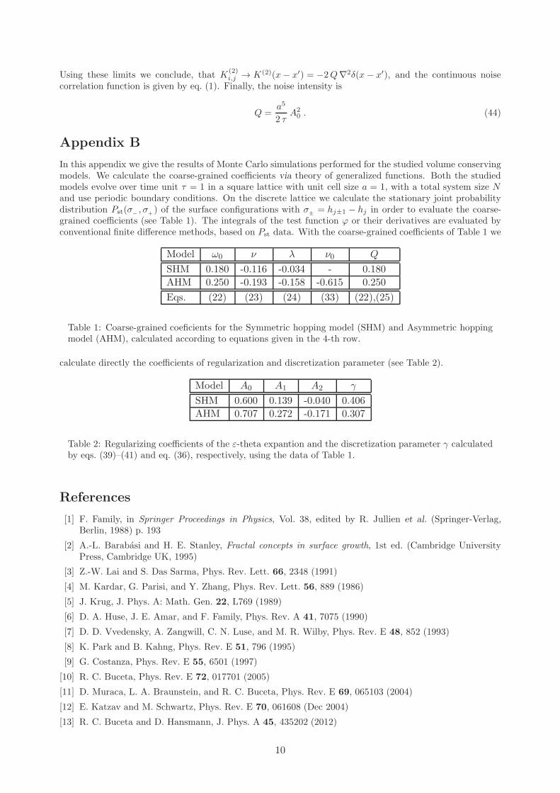
Using these limits we conclude, that K(2)i,j → K(2)(x− x′) = −2Q∇2δ(x− x′), and the continuous noise

correlation function is given by eq. (1). Finally, the noise intensity is

Q =a5

2 τA2

0 . (44)

Appendix B

In this appendix we give the results of Monte Carlo simulations performed for the studied volume conservingmodels. We calculate the coarse-grained coefficients via theory of generalized functions. Both the studiedmodels evolve over time unit τ = 1 in a square lattice with unit cell size a = 1, with a total system size Nand use periodic boundary conditions. On the discrete lattice we calculate the stationary joint probabilitydistribution Pst(σ−

, σ+) of the surface configurations with σ

±= hj±1 − hj in order to evaluate the coarse-

grained coefficients (see Table 1). The integrals of the test function ϕ or their derivatives are evaluated byconventional finite difference methods, based on Pst data. With the coarse-grained coefficients of Table 1 we

Model ω0 ν λ ν0 Q

SHM 0.180 -0.116 -0.034 - 0.180

AHM 0.250 -0.193 -0.158 -0.615 0.250

Eqs. (22) (23) (24) (33) (22),(25)

Table 1: Coarse-grained coeficients for the Symmetric hopping model (SHM) and Asymmetric hoppingmodel (AHM), calculated according to equations given in the 4-th row.

calculate directly the coefficients of regularization and discretization parameter (see Table 2).

Model A0 A1 A2 γ

SHM 0.600 0.139 -0.040 0.406

AHM 0.707 0.272 -0.171 0.307

Table 2: Regularizing coefficients of the ε-theta expantion and the discretization parameter γ calculatedby eqs. (39)–(41) and eq. (36), respectively, using the data of Table 1.

References

[1] F. Family, in Springer Proceedings in Physics, Vol. 38, edited by R. Jullien et al. (Springer-Verlag,Berlin, 1988) p. 193

[2] A.-L. Barabasi and H. E. Stanley, Fractal concepts in surface growth, 1st ed. (Cambridge UniversityPress, Cambridge UK, 1995)

[3] Z.-W. Lai and S. Das Sarma, Phys. Rev. Lett. 66, 2348 (1991)

[4] M. Kardar, G. Parisi, and Y. Zhang, Phys. Rev. Lett. 56, 889 (1986)

[5] J. Krug, J. Phys. A: Math. Gen. 22, L769 (1989)

[6] D. A. Huse, J. E. Amar, and F. Family, Phys. Rev. A 41, 7075 (1990)

[7] D. D. Vvedensky, A. Zangwill, C. N. Luse, and M. R. Wilby, Phys. Rev. E 48, 852 (1993)

[8] K. Park and B. Kahng, Phys. Rev. E 51, 796 (1995)

[9] G. Costanza, Phys. Rev. E 55, 6501 (1997)

[10] R. C. Buceta, Phys. Rev. E 72, 017701 (2005)

[11] D. Muraca, L. A. Braunstein, and R. C. Buceta, Phys. Rev. E 69, 065103 (2004)

[12] E. Katzav and M. Schwartz, Phys. Rev. E 70, 061608 (Dec 2004)

[13] R. C. Buceta and D. Hansmann, J. Phys. A 45, 435202 (2012)

10

[14] T. Sun, H. Guo, and M. Grant, Phys. Rev. A 40, 6763 (1989)

[15] J. Villain, J. Phys. I 1, 19 (1991)

[16] J. Krug, Adv. Phys. 46, 139 (1997)

[17] J. M. Lopez, M. Castro, and R. Gallego, Phys. Rev. Lett. 94, 166103 (2005)

[18] Y. Jung and I. Kim, Phys. Rev. E 59, 7224 (1999)

[19] H. A. Kramers, Physica 7, 284 (1940)

[20] J. E. Moyal, J. R. Stat. Soc. B 11, 150 (1949)

[21] N. G. Van Kampen, Stochastic Processes in Physics and Chemistry (North Holland, Amsterdam, 1981)

[22] L. Schwartz, Theorie des distributions, nouvelle ed. (Hermann, Paris, 1966)

[23] J. F. Colombeau, New generalized functions and multiplication of distributions (North Holland, Ams-terdam, 1984) p. 375

[24] D. E. Wolf and J. Villain, EPL 13, 389 (1990)

[25] S. Das Sarma and P. Tamborenea, Phys. Rev. Lett. 66, 325 (1991)

[26] Z.-F. Huang and B.-L. Gu, Phys. Rev. E 54, 5935 (1996)

[27] C. A. Haselwandter and D. D. Vvedensky, Phys. Rev. E 73, 040101(R) (2006)

[28] C. A. Haselwandter and D. D. Vvedensky, Phys. Rev. E 76, 041115 (2007)

Acknowledgements

D.H. thanks to CONICET for its support.

11