Coarse-grain time sharing with advantageous overhead ...

University of Windsor University of Windsor

Scholarship at UWindsor Scholarship at UWindsor

Electronic Theses and Dissertations Theses, Dissertations, and Major Papers

2010

Coarse-grain time sharing with advantageous overhead Coarse-grain time sharing with advantageous overhead

minimization for parallel job scheduling minimization for parallel job scheduling

Bryan Esbaugh University of Windsor

Follow this and additional works at: https://scholar.uwindsor.ca/etd

Recommended Citation Recommended Citation Esbaugh, Bryan, "Coarse-grain time sharing with advantageous overhead minimization for parallel job scheduling" (2010). Electronic Theses and Dissertations. 7964. https://scholar.uwindsor.ca/etd/7964

This online database contains the full-text of PhD dissertations and Masters’ theses of University of Windsor students from 1954 forward. These documents are made available for personal study and research purposes only, in accordance with the Canadian Copyright Act and the Creative Commons license—CC BY-NC-ND (Attribution, Non-Commercial, No Derivative Works). Under this license, works must always be attributed to the copyright holder (original author), cannot be used for any commercial purposes, and may not be altered. Any other use would require the permission of the copyright holder. Students may inquire about withdrawing their dissertation and/or thesis from this database. For additional inquiries, please contact the repository administrator via email ([email protected]) or by telephone at 519-253-3000ext. 3208.

https://scholar.uwindsor.ca/

https://scholar.uwindsor.ca/etd

https://scholar.uwindsor.ca/theses-dissertations-major-papers

https://scholar.uwindsor.ca/etd?utm_source=scholar.uwindsor.ca%2Fetd%2F7964&utm_medium=PDF&utm_campaign=PDFCoverPages

https://scholar.uwindsor.ca/etd/7964?utm_source=scholar.uwindsor.ca%2Fetd%2F7964&utm_medium=PDF&utm_campaign=PDFCoverPages

mailto:[email protected]

Coarse-Grain Time Sharing with Advantageous Overhead Minimization for Parallel Job Scheduling

By

Bryan Esbaugh

A Thesis Submitted to the Faculty of Graduate Studies

through Computer Science In Partial Fulfillment of the Requirements for

the Degree of Master of Science at the University of Windsor

Windsor, Ontario, Canada 2010

© Bryan Esbaugh

1 * 1 Library and Archives Canada

Published Heritage Branch

Bibliothgque et Archives Canada

Direction du Patrimoine de l'6dition

395 Wellington Street Ottawa ON K1A 0N4 Canada

395, rue Wellington Ottawa ON K1A0N4 Canada

Your file Votre reference ISBN: 978-0-494-62741-9 Our file Notre reference ISBN: 978-0-494-62741-9

NOTICE: AVIS:

The author has granted a non-exclusive license allowing Library and Archives Canada to reproduce, publish, archive, preserve, conserve, communicate to the public by telecommunication or on the Internet, loan, distribute and sell theses worldwide, for commercial or non-commercial purposes, in microform, paper, electronic and/or any other formats.

L'auteur a accorde une licence non exclusive permettant a la Bibliotheque et Archives Canada de reproduire, publier, archiver, sauvegarder, conserver, transmettre au public par telecommunication ou par I'lnternet, preter, distribuer et vendre des theses partout dans le monde, a des fins commerciales ou autres, sur support microforme, papier, electronique et/ou autres formats.

The author retains copyright ownership and moral rights in this thesis. Neither the thesis nor substantial extracts from it may be printed or otherwise reproduced without the author's permission.

L'auteur conserve la propriete du droit d'auteur et des droits moraux qui protege cette these. Ni la these ni des extraits substantiels de celle-ci ne doivent etre imprimis ou autrement reproduits sans son autorisation.

In compliance with the Canadian Privacy Act some supporting forms may have been removed from this thesis.

While these forms may be included in the document page count, their removal does not represent any loss of content from the thesis.

Conformement a la loi canadienne sur la protection de la vie privee, quelques formulaires secondaires ont ete enleves de cette these.

Bien que ces formulaires aient inclus dans la pagination, il n'y aura aucun contenu manquant.

M

Canada

Declaration of Originality

I hereby certify that I am the sole author of this thesis and that no part of this thesis has been published or submitted for publication.

I certify that, to the best of my knowledge, my thesis does not infringe upon anyone's copyright nor violate any proprietary rights and that any ideas, techniques, quotations, or any other material from the work of other people included in my thesis, published or otherwise, are fully acknowledged in accordance with the standard referencing practices. Furthermore, to the extent that I have included copyrighted material that surpasses the bounds of fair dealing within the meaning of the Canada Copyright Act, I certify that I have obtained a written permission from the copyright owner(s) to include such material(s) in my Thesis and have included copies of such copyright clearances to my appendix.

I declare that this is a true copy of my thesis, including any final revisions, as approved by my thesis committee and the Graduate Studies office, and that this thesis has not been submitted for a higher degree to any other University or Institution.

iii

Acknowledgements

I would like to express my deep appreciation and acknowledgement to Dr.

Sodan. I would also like to thank my committee members Dr. Schurko, Dr.

Boufama, and Dr. Tsin for spending their precious time to read this thesis and

offer their comments and suggestions toward this work.

iv

Abstract

Parallel job scheduling on cluster computers involves the usage of several

strategies to maximize both the utilization of the hardware as well as the

throughput at which jobs are processed. Another consideration is the response

times, or how quickly a job finishes after submission. One possible solution

toward achieving these goals is the use of preemption. Preemptive scheduling

techniques involve an overhead cost typically associated with swapping jobs in

and out of memory. As memory and data sets increase in size, overhead costs

increase. Here is presented a technique for reducing the overhead incurred by

swapping jobs in and out of memory as a result of preemption. This is done in the

context of the Scojo-PECT preemptive scheduler. Additionally a design for

expanding the existing Cluster Simulator to support analysis of scheduling

overhead in preemptive scheduling techniques is presented. A reduction in the

overhead incurred through preemptive scheduling by the application of standard

fitting algorithms in a multi-state job allocation heuristic is shown.

V

TABLE OF CONTENTS

Declaration of Originality iii Acknowledgements iv Abstract v

1. Introduction 1 1.1 J ob Scheduling 1 1.2 Time Sharing, Space Sharing, and Overhead 2 1.3 Objective 5 1.4 Paper Structure 6

2. Related Work 7

3. SCOJO-PECT Scheduler 12 3.1 Job Submission and Limits of Preemption 12 3.2 Core Scheduling Algorithm 13 3.3 Non-Type Slice Backfilling 16 3.4 Intelligent Node Selection 18

4. Job Allocation Heuristic 21 4.1 Preliminary Concepts 21 4.2 Node Allocation 24

5. Design and Implementation 32 5.1 Cluster Simulator 32 5.2 Node Design and Implementation 32 5.3 Loading and Swapping Jobs 34 5.4 Memory Modelling 36 5.5 Fitting Allocator Classes 40

6. Tests 41 6.1 Experimental Setup 41 6.2 Results and Interpretation 46 6.3 Overall Test Results 51

7. Conclusions and Future Work 53

Appendix A Node.java 55

Appendix B Cluster .allocateJob() 61

Appendix C Fitting Algorithms 64

vi

Appendix D MemoryModel.java 68

Appendix E Job Scheduling Visualization 70

Bibliography 72 Vita Auctoris 75

List of Tables

Table 1 - Scheduling Parameters 43 Table 2 - Workload Characteristics 43 Table 3 - Memory Model Assignment 47 Table 4 - Synthetic Load Test Results - Best-Fit/Worst-Fit 48 Table 5 - Synthetic Load Test Results - Best-Fit/Best-Fit 48 Table 6 - Synthetic Load Test Results - Worst-Fit/Worst-Fit 49 Table 7 Synthetic Load Test Results - Worst-Fit/Best-Fit 49 Table 8 - SDSC-BLUE Workload Test Results 50 Table 9 - LANL-CM5 Workload Test Results 51

List of Figures

Figure 1 - Time Sharing 3 Figure 2 - Ousterhout Matrix 4 Figure 3 - Job Sorting by Runtime 14 Figure 4 - Job Type Time Slices 15 Figure 5 - Filling Slices with Jobs 15 Figure 6 - Non-Type Slice Backfilling 17 Figure 7 - Overhead applied at slice switches 19 Figure 8 - Allocation of Jobs under First-Free 20 Figure 9 - Intelligent Node Allocation Approach 20 Figure 10 - Node Memory Capacity 24 Figure 11 - Node Allocation Conflict 25 Figure 12 - Node Allocation Conflict Resolution 26 Figure 13 - Job Fitting Methods 28 Figure 14 - Job Allocation Heuristic 31 Figure 15 - Partial Job Swap to Disk 35 Figure 16 - Adjustment according to Swap out Cost 36 Figure 17 - Memory Models 37 Figure 18 - LANL-CM5 Workload Memory Requirements 39 Figure 19 - Relative Response Time Calculation 45 Figure 20 - Improvement Calculation Equations 46 Figure 21 - Synthetic Load Comparative Results 50 Figure 22 - Best Fit Allocator Implementation 65 Figure 23 - Worst Fit Allocator Implementation 66 Figure 24 - First Fit Allocator Implementation 67 Figure 25 - Cluster Simulator Visualization 71

vii

1. INTRODUCTION

1.1 Job Scheduling

Analysis and usage of large data sets in reasonable amounts of time

necessitates the need for parallelism in computation. This parallel computation is

often referred to as parallel "jobs" in the context of multi-user clusters. Hardware

capable of running massively parallel jobs is often prohibitively expensive. This

means these resources need to be shared amongst several differing users and

types of jobs. The sharing of computing resources necessitates in turn the need

for effective scheduling algorithms in which the usage of the shared resources

can be most effectively optimized.

Several optimization objectives can be applied to job scheduling. These include:

• Throughput - the number of jobs completed over time

• Response times - the time between a jobs submission and time the job

completes

• Utilization - percentage of the resources used over time

• Quality of Service - the upper limit to the amount of time a job should take

to complete after submission

• Fairness - guarantees the system makes that the job will complete in a

reasonable amount of time

• Deadline Satisfaction - the number of jobs completed before a deadline

l

The predictability of response times for jobs submitted is also associated to

Quality of Service as well as providing a means to explore further optimization

methods.

1.2 Time Sharing, Space Sharing, and Overhead

Each job upon submission, depending on the jobs characteristics, will be

given a certain amount of the processing resources. The amount of resources

and the time at which they are supplied dictate the response time of jobs

submitted. Response time is the amount of time taken between a job submission

and the job being completed. Relative response time is the response time

relative to the runtime of job. For example, if a job's total runtime is 10 minutes

and the response time is 15 minutes, then the relative response time for that job

would be 1.5 (i.e., 15 minutes /10 minutes). One strategy for sharing resources

is to allow jobs certain amounts of time over a period in which to run. In this

strategy jobs are swapped on and off of the resources so that each job in the

system gets a chance to make progress and complete. These types of strategies

are known as "Time Sharing" approaches. In these approaches preemption is

often used to suspend a currently running job so that another job can utilize the

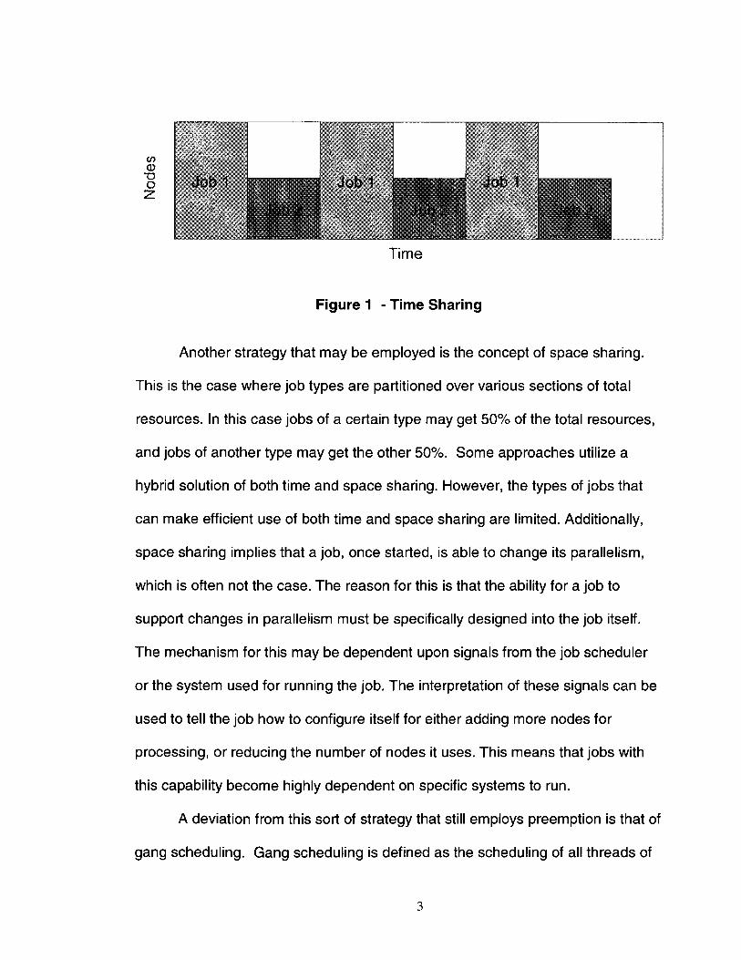
resources. Figure 1 shows Job 1 and Job 2 each taking turns running overtime

(i.e., sharing the available runtime). One of the issues is the overhead incurred

while swapping the job on and off of resources. This is caused by multiple jobs

being allocated to the same resources while not being able to fit together in

memory. This means that one or more jobs must be swapped out in order for the

job whose turn it is to run.

2

CO CD

TJ O

Time

Figure 1 - Time Sharing

Another strategy that may be employed is the concept of space sharing.

This is the case where job types are partitioned over various sections of total

resources. In this case jobs of a certain type may get 50% of the total resources,

and jobs of another type may get the other 50%. Some approaches utilize a

hybrid solution of both time and space sharing. However, the types of jobs that

can make efficient use of both time and space sharing are limited. Additionally,

space sharing implies that a job, once started, is able to change its parallelism,

which is often not the case. The reason for this is that the ability for a job to

support changes in parallelism must be specifically designed into the job itself.

The mechanism for this may be dependent upon signals from the job scheduler

or the system used for running the job. The interpretation of these signals can be

used to tell the job how to configure itself for either adding more nodes for

processing, or reducing the number of nodes it uses. This means that jobs with

this capability become highly dependent on specific systems to run.

A deviation from this sort of strategy that still employs preemption is that of

gang scheduling. Gang scheduling is defined as the scheduling of all threads of

3

a process or job at the same time [10] [22]. The threads of the running job are

allocated to separate nodes. In gang scheduling, all time slices are globally co-

ordinated and all threads of a running job are preempted if another job gets its

turn to run on the allocated resources. Gang scheduling is always combined with

space allocation per time slice, organized by use of an Ousterhout matrix [18].

Node 1 Node 2 Node 3 Node 4 Slot 1 Job A Job A Job A Job A Slot 2 Job B Job B Job C Job C Slot 3 Job A Job A Job A Job A Slot 4 Job B Job B Job D Job D Repeat cycle

Figure 2 - Ousterhout Matrix

In this matrix, as shown in Figure 2, the columns represent the available

nodes while the row represent the differing time slices, or slots. Each time slice

has a list of one or more gangs. In Figure 2, slot 1 has a gang consisting of just

Job A consuming 4 processors. Slot 2 has a gang consisting of Job B, and Job C

each consuming two processors. Each available slot that has an assigned gang

gets a period of time in which to run, one after the other. In this approach, there

is no swap between jobs allocated to the same resources. This means that each

node incurs high levels of memory pressure due to concurrently allocated jobs.

Only jobs that all fit into memory can share resources.

Any scheduling method incurs some overhead in order to implement the

algorithm. This overhead can, in the case of time-sharing, include the cost to stop

and restart a running job. This is usually manifested by the memory costs to load

4

a new job into memory. As well, this can be seen in the time taken to swap a

preempted job out to disk and swap a previously stopped job back in. In the case

of space sharing, this overhead may be manifested by the time taken to

reconfigure the parallelism characteristics of a job that is to be given runtime. The

parallelism characteristics are defined as the number of nodes, or processors,

required by a running job. Reconfiguration of these characteristics means

changing the number of nodes a job runs on (e.g., going from 10 nodes to 8

nodes). This thesis will focus only on a time-sharing based scheduling approach.

1.3 Objective

The focus and contribution of this thesis is to detail a new method designed

to effectively allocate parallel jobs to resources. The design of this method is

such that the overhead due to memory swap costs is minimized in the context of

a coarse grained time-sharing job scheduler. Each job to be scheduled

consumes an amount of memory from the group of nodes over which it is

running. Several jobs of differing types may be assigned to overlapping groups of

nodes in which they each receive a share of the total runtime. The overhead is

manifested when the group of jobs assigned to common processing nodes

cannot all simultaneously fit into memory.

Previous exploration into methods designed to increase overall

performance of the scheduling algorithms did not take into consideration a higher

fidelity model of memory interaction or ways to reduce the memory swap

overhead [6][7]. The new algorithms presented are implemented as an extension

of the existing Scojo-PECT scheduler [6] [7], The Scojo-PECT scheduler is a

5

time-sharing preemptive scheduler for scheduling parallel jobs on computing

clusters. The Scojo-PECT scheduler and scheduling algorithm is implemented as

part of a cluster simulator framework used for analysis of scheduling methods

and algorithms.

1.4 Paper Structure

The rest of this thesis is organized as follows. Chapter 2 reviews some

previous work in the area of memory and overhead reduction for job scheduling.

Chapter 3 further details the Scojo-PECT Scheduler and Cluster Simulator. This

cluster simulator has been modified to account for job and processor node

memory considerations. Chapter 4 explains the mechanism and overall algorithm

for job allocation. Chapter 5 details the design and implementation of supporting

additions to the Scojo-PECT simulator. Chapter 6 details the test cases and

results. Chapter 7 concludes this work with an interpretation of the results and

mentions possible future work in this area.

6

2. RELATED WORK

Much of the previously detailed research in parallel systems and job

scheduling has focused on how to improve the performance of single

applications running in isolation. The only global concern has been on producing

feasible schedules that can satisfy release times, deadline constraints, and

minimization of the total schedule times. While minimization of total schedule

time may negatively affect the response time of a single job, we still view these

jobs as separate from each other and not dependent on the processing of other

jobs on other processors.

Some areas of research have explored the topic of memory management

in the context of parallel processing [4]. This research has specified that memory

management is hardly exercised due to the performance implications on parallel

jobs and the effect on synchronization. Parallel jobs must be completely memory

resident in order to execute. Research into this area has been slowed by lack of

actual information about the memory requirements that are experienced in

practice. Some observations from this work include that many jobs use a

relatively small part of the memory available on each node so that there is room

for preemption among several memory resident jobs. As well, larger jobs tend to

use more memory but it becomes difficult to characterize the scaling of per-

processor memory usage.

Other research has produced an approach for real time multiprocessor

scheduling which reduces preemption related overhead. This is done by reducing

the number of preemptions as compared to an algorithm that performs

7

preemptions at set time periods [11]. The main idea in this approach is to be

aware of newly arriving jobs in the queue available for running on a set of

resources such that if there were no newly arriving jobs, the cost of preemption

could be eliminated. This would be similar to the way the current Scojo-PECT

scheduler works in that after a scheduling decision is made as to where jobs will

run in the next time period after preemption, only jobs that are actually

preempted incur any overhead costs.

Further research explores the maximum gain that can be realized by

increasing the number of preemptions in a multiprocessor system [14]. This

research considers the possibility of jobs which may be preempted at any point in

time. Additionally, the job may be split into two parts or relocated to different

processors. These methods seek to balance the gain that can be realized by

increasing the number, and timing, of preemptions against the overhead cost of

the preemption. These preemptions are triggered as jobs finish or new jobs

arrive. For certain types of systems the cost of preemption in can be relatively

inexpensive. These systems include shared memory multiprocessor machines.

However, in other sorts of systems the cost for preemption is high and so the

decision to preempt must be weighed against keeping the load reasonably

balanced and the overhead incurred by preemption. These systems include non-

shared memory multi-processor machines and distributed systems. The Scojo-

PECT scheduler uses preemption primarily to allow shorter jobs runtime where

they would otherwise be blocked by longer running jobs consuming the

8

resources. This provides a better quality of service for shorter jobs as they would

have quicker access to resources on which to run.

Other sorts of scheduling methods do not consider preemption but rather

simply attempt to fill in gaps in the schedule. One method describes a scheduling

solution which attempts to find the earliest gap in a schedule in which a newly

arriving job will fit [15]. This is further augmented by use of a Tabu search to fill in

gaps by using the last job in a schedule of a machine that has the highest

number of delayed or waiting jobs. Tabu search is an algorithm for solving

combinatorial optimization problems. It uses an iterative search method which

proceeds until a stopping criterion has been satisfied. A typical stopping criterion

may be a certain number of iterations being performed. In order to prevent the

iterations from producing cycles of similar solutions, an attribute of each solution

that results from each iteration is kept in a "tabu" list. This is used to prevent

previously found solutions from reappearing and causing cycles in the search

space. In this approach, preemption is not supported. Jobs may still experience

starvation even though this effect is somewhat mitigated by attempting to

balance deadlines against schedule priority. This is done by placing each job in a

machine schedule in order of earliest deadline. The net effect is similar to serving

shorter jobs, with earlier deadlines, in preference of longer jobs, with later

deadlines.

Other approaches examine the difference in scheduling methods and

performance by using algorithms that set broader timeframes [16]. The

timeframes are called "prime-time" and "non-prime time". Larger jobs are

9

relegated to non-prime times. In the examination of this approach it is determined

that setting limits for jobs that may run in prime time has beneficial effects for

batch scheduling in among other backfilling methods such as EASY and first

come first serve. A problem with this approach is that setting limits for job types

allowable to be run in prime time is difficult due to competing needs of large and

small jobs.

Other research explores a tuneable selective suspension scheduling

heuristic based on the generation of an expansion factor for jobs [13]. As a job

waits for runtime its expansion factor increases. Once this factor exceeds a

threshold, a set of jobs is selected for preemption based on a set of criteria. This

method does allow the migration of jobs to different nodes in the system and as

such can offer more options for fitting jobs together. However this relocation does

incur an overhead. In this research the memory requirement for jobs is estimated

to be randomly and uniformly distributed between 100MB and 1GB. The actual

memory size of the computing resource is less important in this research. This is

because the bulk of the overhead costs are related to migration. Migration

requires that a job be preempted so the overhead cost is incurred in any case.

Preemption to disk is required before a job can be migrated to new nodes. This

means that the ability to keep jobs in memory together is less important to this

method. The overhead for preemption is calculated as the time taken to write the

main memory used by the job to disk. The evaluations of this method observed

that overhead does not significantly affect the performance of the algorithm.

10

Further research states that preemption related overhead may cause

"undesired high processor utilization, high energy consumption, and in some

cases, even infeasibility" [5]. Considering this, the approach chosen in this

research is a method for limiting the number of preemptions in legacy fixed

priority scheduling. Fixed priority scheduling methods are composed of systems

consisting of tasks, priorities, periods and offsets. In this case the algorithm

knows about the tasks or jobs in advance. Priorities and offsets are then

analyzed and re-assigned. This is done to minimize the number of preemptions,

and therefore the preemption overhead. This differs from the other approaches in

that it considers an offline set of jobs. An offline set of jobs is where the

scheduler has prior knowledge and complete information about the jobs to be

scheduled.

11

3. SCOJO-PECT SCHEDULER

3.1 Job Submission and Limits of Preemption

Jobs are simulated to be submitted to the cluster simulator and the

scheduler at non-deterministic times. This means the scheduler has no prior

knowledge about when or what type of jobs may arrive. This is in contrast to job

scheduling systems where we may have all or most of the relevant information.

Scheduling approaches that have all prior information about the jobs to be

scheduled falls under the category of "offline" or deterministic scheduling. In

these cases there exist many algorithms and research addressing the offline

scheduling problem. In the context of job scheduling on compute clusters,

completely off-line scheduling problems are usually an analysis of an artificial

theoretical case. This means that in practical usage, we almost never have all

knowledge or information about jobs to be scheduled on a computer cluster. The

case we consider in this thesis is that of "online" or non-deterministic scheduling

where we do not have all the required information to produce an optimal

schedule. In these cases, as jobs are submitted we must make decisions based

upon the state of the schedule at a certain point in time with consideration

towards certain performance objectives.

In evaluating the performance of an offline scheduling heuristic it is

sometimes possible to measure an optimality function or performance objective

against a hypothetical offline solution for the same job set and measure the ratio

of performance or competitiveness of the online algorithm to the optimal offline

solution. In cases where calculating an optimal off-line solution is either NP-Hard

12

or NP-Complete we can still compare an online solution with the best known

offline algorithm for competitive analysis [21]. Unfortunately, it is often the case

that scheduling problems become NP-Hard whenever more than two processors

are utilized [1]. Additionally, in cases where we have no prior knowledge about a

jobs deadlines, computation time and or start times, then for any sort of

scheduling algorithm we may use, one can always find a set of jobs which can be

better scheduled by another algorithm [4]. In the case of preemptive online

schedulers, at least as far as minimization of schedule completion times, there

may be limits to how well you can actually schedule jobs, as indicated by work in

[2] which attempts to derive a lower bound on the competitiveness of preemptive

online scheduling heuristics.

In the case of the Scojo-PECT scheduler, the core scheduling algorithm

used in the simulator is primarily concerned with balancing response time across

job types in a non-deterministic or online context. Within this framework this

paper explores preemption overhead minimization within the context of the

overall scheduling heuristic. As each job is submitted it is sorted into one of three

categories, short, medium, or long, based on estimated runtime. After this sorting

each job is scheduled according to the assigned scheduler heuristic

(implemented as a scheduler object) within the simulator.

3.2 Core Scheduling Algorithm

The basic approach of the Scojo-PECT scheduler utilizes coarse-grain time

sharing. Each time period is divided up into slices in which jobs of differing types

may be allocated resources and run. As previously mentioned, the only division

13

for scheduling slices is based on a job's estimated runtime. So, jobs are divided

into short, medium and long categories (Figure 3).

i ^ \

Short

t Long

Figure 3 - Job Sorting by Runtime

Each category is given an amount of time each interval (Figure 4). An

interval is an amount of time which is divided into slices for each job category.

For example, each interval period is divided into a long job slice, a medium job

slice and short job slice. In the Scojo-PECT scheduler the interval period is

configurable between 30 minutes and 60 minutes. This allows exploration into

scheduling methods using more or less frequent preemptions. If the interval time

is shorter, more slices are scheduled in a shorter amount of time.

14

Time (30min - 1 hr)

Figure 4 - Job Type Time Slices

Jobs are scheduled in a first come first serve basis in their respective time

slice. That is, short jobs are scheduled to run in the short slice, medium jobs are

scheduled to run in the medium slice, and long jobs are scheduled to run in the

long slice. Jobs may be backfilled into a slice not of their type to exploit free

resources, but in all cases jobs of the slice type have priority for the resources in

that time slice. For example, in a long slice, all long jobs have priority for

resources over jobs of any other type. Resources refer to computing nodes in the

cluster unless otherwise specified. Figure 5 shows the scheduling of jobs in

slices of differing types.

Short Medium Long

m i l l B I I I

Time (30min - 1 hr)

Figure 5 - Filling Slices with Jobs

15

Backfilling means that jobs may move ahead in the order of submission if

they do not delay other jobs as specified by the backfilling approach. Scojo-

PECT can utilize either conservative or EASY (the Extensible Argonne

Scheduling System) backfilling. Conservative backfilling means that none of the

jobs in the queue are delayed by a job moved ahead of their normal first come

first serve position. EASY backfilling is less restrictive in that only the first job in

the waiting queue need not be delayed as compared to its position in the

schedule at submission time.

3.3 Non-Type Slice Backfilling

The Scojo-PECT scheduler implements a unique type of EASY and

conservative backfilling in the context of separate job slices [6] [7]. Non-type slice

backfilling refers to backfilling jobs of a different type than the currently scheduled

slice onto free resources that exist in that slice (e.g., backfilling a short job onto

free nodes that exist in a long slice). The restrictions on non-type slice backfilling

are the same as normal backfilling. Any backfilled job must not delay any job of

its own type that has arrived at the system ahead of it. This means a later arriving

job may not delay a job of the same type that arrived prior to it as a result of

being backfilled. The EASY version of this sort of backfilling is less restrictive.

Under EASY the only restriction is that jobs may not delay the first job of its type

in that job types queue. For instance, if the first job in the short job queue cannot

be scheduled due to lack of resources a later arriving short job needing fewer

16

resources may be backfilled ahead of it. Under EASY, this is only allowed if the

backfilled job does not delay the first job.

These restrictions are applied even if the job to be backfilled is consuming

resources in a slice not of its type. For example, a short job may be backfilled

into free space in a long slice as long as this action does not delay any short job

arriving previous to the job that is backfilled. Figure 6 shows short jobs being

backfilled into medium and long slices.

Medium

Time (30min - 1 hr)

Figure 6 - Non-Type Slice Backfilling

With all backfilling in Scojo-PECT, jobs of the slice type have priority and

are the first considered backfilling candidates. Any preempted jobs from other

slices that can fit onto any free resources are the next candidates for backfilling.

Preempted jobs must only be backfilled onto resources which they were originally

allocated. Scojo-PECT does not consider migration of jobs to new resources.

This is then followed by waiting jobs from other slices. Waiting jobs may be

scheduled on any free resources as long as this does not create resource

conflicts within the jobs slice type. The consideration is done in order of

17

increasing runtime length. For example, while backfilling into a long slice, short

preempted jobs are considered as backfill candidates before medium preempted

jobs. Then short waiting jobs are considered before medium waiting jobs. In all

cases backfilling is not permitted to create any conflicts over resources with other

jobs in their own slice type (i.e. the job needs to finish before the end of the slice

in which it is backfilled, or run on resources which are not yet allocated in the

slice of their own corresponding type).

3.4 Intelligent Node Selection

Previous versions of the Scojo-PECT scheduler assigned nodes in each

slice based on the first found available nodes, or the "first-free" approach. The

"first-free" approach is defined as the allocating a job to the first nodes (i.e.,

resources) that are available in the slice on which the job may run. In this

approach there is no consideration other than the availability of the nodes in the

slice. An improvement to Scojo-PECT over the first-free method attempts to

intelligently allocate jobs on nodes which are not yet allocated to any job in any of

the slices [6]. This is defined as the "intelligent node selection" method. This

method simply counts the number of jobs allocated to run in other slices on the

available nodes in the current slice. Nodes are then allocated to the job under

consideration (i.e., the waiting job to be scheduled) in order of the lowest count

per node. For example, a node having no other job allocated to it in any other

slice would be allocated to the job under consideration before a node having one

or two other jobs allocated to it in other slices. This increases the likelihood of

jobs being able to backfill into other slices. This is because we are intentionally

18

seeking to reduce the possibility of conflict for resources across time slices. A

side effect not considered in the original design of this method was the saving in

overhead this would provide over the "first-free" approach. This was due to the

fact that the original modelling of the cluster did not account for overhead on a

per job basis, but rather applied a global overhead to all running jobs during slice

switches. Figure 7 shows preemption overhead as applied universally at slice

switches. The overhead is incurred during the time represented by the thick lines

at the end of the time slices.

Figure 8 shows how jobs across slices would be allocated according the

first-free approach. With this sort of allocation, there is no possibility for non-type

slice backfilling as each job consumes the same resources. All jobs must wait

until their next slice to complete processing.

Figure 7 - Overhead applied at slice switches

19

Short Medium Long

Time (30min - 1 hr)

Figure 8 - Allocation of Jobs under First-Free

Figure 9 shows how jobs are allocated using the intelligent node selection

approach. In this case each job is allocated to nodes that are not in conflict

across slices. This allows jobs to backfill and complete in other slices rather than

being blocked.

Short Medium Long

<f> CD "U O

Time (30min - 1 hr)

Figure 9 - Intelligent Node Allocation Approach

20

4. JOB ALLOCATION HEURISTIC

4.1 Preliminary Concepts

As previously mentioned, jobs are submitted to the scheduler at non-

deterministic times. As each job gets submitted to the job scheduler, it is sorted

into a waiting queue based on its type (short, medium, or long) at which point it

waits until it is scheduled in a slice corresponding to the job type that is to be run

As previously mentioned, a waiting job may also be initially started as a result of

backfilling. In all cases we assume perfect estimates for the runtime of jobs. The

job types are determined by definition within the scheduler based on runtime.

This means that within the scheduler, jobs are defined as being in one of the

three categories based on the configuration of the scheduler (e.g., Scojo-PECT

currently defines short jobs as jobs with runtimes less than 10 minutes). At this

point each job of that type is placed in a running queue, in first come, first serve

order on the available resources for that job. In the case where the number jobs

of that type need more resources than are currently available, the later arriving

jobs must wait until earlier jobs finish and the resources become free. As

previously mentioned, jobs may have opportunities to backfill into other slices if

nodes are available. Before jobs can be set to a running state, they need to be

allocated resources on which to run. These resources consist of the simulated

processing nodes on which the "tasks" of the parallel job run. That is, if a job is

submitted and requires 24 nodes on which to run, the actual 24 nodes of the

cluster the job will run on must be determined. All "tasks" of a parallel job in this

21

model are assumed to be identical in time required and memory utilized. This

approximates a situation where the parallelism of the job is good and that all

running tasks are required to complete the job. All jobs are considered to be

unique in that a program running with data set A and the same program running

with data set B are considered to be two distinct jobs. This is because a program

or application may behave quite differently given two distinct data sets. An

example of this would be a numerical analysis application which converges to

local minima quickly given one set of data. With another set of data the same

program may only converge to local minima after a long period of time.

All nodes in the system are homogeneous in that each node has identical

performance and memory characteristics. This means that the memory available

in each node is consistent and the time to load/swap a job to or from disk is the

same across all nodes. In this model it is assumed that no migration is possible

for jobs that have started running. This means that once a job's nodes have been

decided and some processing has started a job may not switch to other nodes.

As well, each job may not change the number of nodes it needs for processing.

If a job requires 12 nodes for processing, but only 10 are available, the job must

wait until such time as 12 nodes are available to either start, or continue

processing. Jobs of this sort are characterized as being "rigid". On each node

only one job may be running at any point in time. Our model and simulator

considers each node to be a single processing unit capable of processing only a

single job at any one time.

22

As jobs are preempted, new jobs will be run on the same nodes. The

preempted jobs may need to be swapped to disk from memory. This would occur

if there is not enough available space to concurrently keep all jobs allocated to

that node, or group of nodes, in memory. Additionally there is a load time

associated with each job corresponding to the amount of time it takes to load

each job into memory for running. This time is the overhead caused by the

memory requirements of the job and the performance characteristics of the node,

namely, the time it takes to swap a job from memory to disk. Overhead can be

reduced by allocating jobs to nodes such that they do not compete for the

resources or limit the amount of swaps needed to keep currently running jobs in

memory.

Allocating jobs to nodes such that conflict over resources is minimized

provides more opportunities for jobs to backfill and take advantage of available

nodes outside their own designated slice. By minimizing conflict across slices,

there is a higher likelihood that jobs will not be allocated the same nodes. This

means that a short job may be backfilled into a long slice and thereby be able to

finish in less time given that the nodes are free in the long slice. This results in

less overhead since the short job would not be required to preempt or swap to

disk. As previously mentioned, the preliminary heuristic addressing node conflict

minimization in Scojo-PECT is the intelligent node selection method. This method

does not consider the memory requirements or characteristics of running jobs.

The allocation method presented in this thesis attempts to reduce overhead

produced by swapping jobs in and out of memory. This is done by attempting to

23

limit the number of cases where the memory requirements of jobs allocated to

resources exceeds the memory of the resources.

° £ tz TO r Q-| «

2 3 Nodes minimise

these cases

Figure 10 - Node Memory Capacity

Figure 10 shows a series of nodes. Jobs are allocated to these nodes and

consume an amount of the nodes memory. A group of jobs allocated to a node

may exceed the memory capacity of the node as shown in Figure 10 on Nodes 7

and 8. These are the cases we are trying to minimize as they will result in the

overhead associated with swapping jobs between memory and disk.

4.2 Node Allocation

Once a job slice type is started, jobs of that type that have been previously

preempted are reallocated to the nodes on which they were previously running.

New waiting jobs that have not had any run time are then allocated to nodes

based on a first come, first serve allocation. Jobs are only allowed to be started

out of order if they will not impact the running of jobs ahead of them in the queue.

24

Once the determination is made that a waiting job will be given runtime it is then

allocated nodes on which to run. The determination that a job be given runtime

may be made based on position in the queue or by backfilling.

The first criterion in determining if a job can be allocated nodes is whether

there are currently enough free nodes available for the job. This means that

enough nodes are available that do not have currently running jobs already

assigned to them. If this is the case then the next step is to determine the best

nodes on which the job should run. From the list of free nodes available (i.e., the

list of nodes without currently running job), a list of nodes with enough free

memory to load the job is created. If the job is starting as a result of a backfilling

decision it is possible that the created list of free nodes contains nodes that are

already allocated to jobs of the same type as the one to be started. These jobs

would normally run in their own slice. In this case, these nodes are excluded from

the newly created list of free nodes. If a job was allowed to be allocated to these

nodes it would result in conflicts in its own slice.

Short Medium Conflict

Long Short

Time (30min - 1 hr)

Figure 11 - Node Allocation Conflict

25

In Figure 11, Job 2 is a short job and would normally be scheduled to run in a

short slice. This job has been backfilled into the medium slice and has been

placed on nodes that are already being utilized by Job 1 in the short slice.

Neither of these jobs has completed and will require more runtime in the next

short slice to finish. During the next short slice, both jobs attempt to resume

running on the same nodes and creates a conflict condition.

Short Medium L o n g S h o r t

T i m e ( 3 0 m i n - 1 hr)

Figure 12 - Node Allocation Conflict Resolution

In Figure 12, Job 2 is only allowed to be allocated to nodes that are not

already being used by jobs of the same type (i.e., no nodes being used by other

short jobs). This ensures that when Job 2 is backfilled into the medium slice it

does not use the nodes already in use by Job 1. During the next short slice both

Job 1 and Job 2 can resume running as there is no conflict over the nodes.

For the nodes remaining in the created list we keep track of the total

amount of memory is currently used in each node. From the list of initial

candidate nodes we find a group of nodes with immediately available memory for

26

the job, (i.e., free nodes with enough free memory to hold the job as well as the

other jobs currently allocated to that node). If there are enough nodes from this

initial listing for the job, the job is assigned nodes from that grouping based on a

best-fit allocation. The general best-fit algorithm in described in Appendix C,

Section 1.

The best-fit allocation is in relation to the amount of available memory on

the node such that the amount of free space left after the allocation on the nodes

in minimized in each node. This is in contrast to a "worst-fit" method. Worst-fit

allocation attempts to place jobs on nodes such that the remaining free memory

after job placement is maximized. These two methods are refinements over a

basic "first-fit" allocation method. First-fit places jobs on the first nodes that are

identified with enough space to hold the job. Figure 13 shows the allocation of a

job (i.e., Job 1) according to the three described fitting methods. In Figure 13,

Job 1 is allocated to Nodes 2 and 6 under the best fit method since these nodes

provide the best fit for the job and minimizes the available space on those nodes.

Using worst fit allocation Job 1 is allocated to Nodes 1 and 5. This is because

these nodes maximize the available space on the individual nodes after the

allocation. Using first-fit, Job 1 is allocated to Nodes 1 and 2 since these are the

first nodes discovered in which Job 1 will fit.

27

1 2 3 4 5 6 7 3 Nodes

'•/Vest F i tA l l o : a t i o r

8

s t ™ L J 5 £ S. ---- j s o — |

1 2 3 4 5 6 7 Nodes

Figure 13 - Job Fitting Methods

The reason for the initial choice of "best fit" of jobs is because we seek to

keep as much free space as possible on nodes for other incoming jobs.

Therefore, we seek to maximize the total available space on each node. This is

opposed to evenly balancing the amount of memory used on each node, or

keeping a little space on each. This is referred to in the test results as the "first

stage" fitting heuristic. For purposes of experimentation the actual fitting

algorithm used at this stage of node allocation is configurable in the

implementation between "best-fit", "worst-fit" and "first-fit". The fitting algorithms

are described in more detail Appendix C.

- i r s t Fit Al locat ion

3

28

If the amount of free nodes found from this initial search is insufficient to run

the job then we have a case where the job must be allocated to a node where, in

order to run the job a previously running job must have part of its memory

allocation swapped out to accommodate the incoming job. In this case we create

a group of nodes that do not have enough available memory to hold all the jobs

that have been allocated and the incoming job together in memory. It is important

to note that generally only jobs of differing types (small, medium, and long) can

be co-allocated to nodes simultaneously. Jobs of the same type are not allowed

to interfere with currently running jobs in their own slice. This means that two jobs

of the same type being scheduled in the same slice cannot overlap on nodes.

This also means that nodes, during periods of high workloads, will contain in

memory jobs from small, medium and long types.

It is known that whatever allocation is chosen at this point will incur the

expense of loading the job in at least one node. This is because it was previously

determined that there were insufficient nodes available with enough free memory

to prevent swapping out jobs. It is also known, according to our model, that jobs

cannot start processing until all tasks of a job have been loaded into memory.

Therefore, it makes more sense to try to allocate the job first on nodes which

cannot contain the job, leaving free nodes available for future incoming jobs.

Overhead from swap cost is incurred in any case and so an attempt to assign

nodes exclusive to nodes without enough free memory is made.

The nodes without enough available memory are then ranked based on the

time until all jobs currently allocated and the new incoming job all fit together in

29

memory. This is essentially the time until one or more of the jobs finish and the

remaining jobs, including the incoming job, can all fit into memory. This is

referred to as the "time until fit". These nodes are allocated even if the number of

"unfree" nodes is less than the number required by the job. Even though the

method does not explicitly determine the amount of memory becoming available

at each time delta, this would not matter as the idea is to minimize the time until

all the jobs fit. All jobs fitting in the nodes memory reduces the number of swaps

and the total overhead incurred.

If the job still is not fully allocated (i.e., still needs nodes to run) then the

remaining nodes are allocated according to a "worst-fit" memory allocation

method. This is referred to in the test results as the "second stage" fitting

algorithm. The reason to use this is that at this stage we know that there is an

insufficient amount of nodes to fully hold wide jobs consuming a high amount of

nodes. Otherwise the job would have been allocated to "free" nodes. Any future

job will in the immediate case encounter the same problem unless it is narrow.

Narrow jobs consume a low number of nodes. Therefore we initially seek to

utilize worst fit in order to ensure that as many nodes as possible have free

memory since narrow jobs tend to use less memory as a general trend. The

choice of using a worst-fit allocation method versus best-fit allocation method at

this stage again is configurable in the implementation for experimental purposes.

The algorithm is detailed in Figure 14. The actual code that corresponds to this is

contained in Appendix B.

30

Proc

freeNodes [ ] //Nodes w i t h enough f r e e memory t o hold job n o d e L i s t [ ] //Nodes w i thou t enough f r e e memory t o run job ex t r aNodeL i s t f ] / * E x t r a node l i s t f o r ho ld ing remaining f r e e nodes a f t e r p a r t i a l assignment*/ i n d i c i e s [ ] / / A r r a y the s i ze o f the number o f nodes requ i red by the job totalMemoryUsedlnNodef] / / A r r a y equal t o the number of nodes i n c l u s t e r preemptedDobsf] / / A r r a y f o r con ta in ing the preempted jobs i n the c l u s t e r allPreemptedDobs / / L i s t o f a l l preempted Dobs i n c l u s t e r c l u s t e r / / the c l u s t e r running the jobs j ob / / The job t o a l l o c a t e nodes t o

runningQueue / / The cu r ren t Running Queue con ta in ing the c u r r e n t l y running j o b s .

Begin preemptedDobs.add ( runningQueue.getDobs() ) ; / / Add a l l running jobs totalMemoryllsedlnNodef ] = getMemoryUsedInNodefromAllDobs( preempted Jobs) ; freeNodes = getL is tOfFreeNodes() ; / /Ge t the l i s t o f f r e e Nodes

i f ( f reeNodes.s ize > job.nodesRequired) {

SortByFreeMemorySize(freeNodes); / / Best F i t

f o r ( i = 0 ; i < job.nodesRequired && i < f reeNodes.s ize ; i++ { i n d i c i e s [ i ] = f reeNodes [ i ] .ge tNode lD j

}

} e lse i f {

nodeList = getL is tOfUnfreeNodes() ; / / L i s t o f nodes w i thou t enough f r e e memory }

fo reach ( j o b i n allPreemptedDobs) { f o r ( ind = 0; ind < job.nodesRequired ; ind ++ ) {

fo reach (node i n j ob ) { i f (node.soonestReleaseTime > job.estimatedResponseTime )

node.soonestReleastTime = job.estimatedResponseTime; }

}

Sor tNodeL is tByT imeUnt i lRe leased(node l is t ) ;

f o r ( i = 0; i < n o d e L i s t . s i z e && i < job.nodesRequired ; i++ ) { i n d i c i e s [ i ] = n o d e L i s t [ i ] ; / /Ass ign node t o l i s t o f i n d i c i e s .

} I f ( n o d e l i s t . s i ze < job.nodesRequired) {

fo reach (node i n c l u s t e r ) { i f ( ! ( n o d e l i s t conta ins node) ) {

ex t raNodeLis t .add(node) ; }

} }

SortByFreeMemorySize(extraNodeList) ; / /Wors t F i t

i n d i c i e s [ ] = assignNodesFromExtraNodeList(); / / A s s i g n the j ob t o nodes }

Dob.ass ignNodes( ind ic ies) ;

Figure 14 - Job Allocation Heuristic

31

5. DESIGN AND IMPLEMENTATION

5.1 Cluster Simulator

The cluster simulator is based on an event-based simulator engine which

simulates the arrival of jobs to a simulated cluster. In the simulation the complete

workload model is created, either from a synthetic model based on the Lublin-

Feitelson workload model [17], or from workload traces from the Feitelson

workload archive [8]. The workload model is used to create a series of job

submissions and times which are placed on an event queue. Each event in the

queue is processed, in some cases creating more events, which are then placed

on the queue and sorted by simulation time of occurrence. Once all the events in

the event queue have been processed, the simulation has ended. All jobs within

the cluster simulator are scheduled according to the core Scojo-PECT scheduling

algorithm [6] [7],

5.2 Node Design and Implementation

In order to support the analysis and testing of overhead and simulate the

effects memory constraints and memory swap costs, the original cluster

simulator source code was modified to support these simulations. The original

cluster simulator had a very basic model for node allocation which consisted of

an array used primarily to mark which nodes were currently occupied. For the

purposes of the investigations in this paper the simulation of actual nodes was

redesigned and implemented for the modified cluster simulator.

32

Instead of a simple array representing nodes in the cluster, a node object

was implemented. Each node object was designed in such a way that they

possessed attributes such as memory size, and transfer rate. The size of the

memory is set as a simple integer associated with the transfer rate. Since

memory size is always relative to job memory requirement and transfer rate the

representation of these attributes in terms of integers is sufficient for simulation.

Additionally, each node was given a "state" attribute which indicates the state of

the node at any time during the running simulation. The possible states include:

• Free - this indicates merely that the node is not currently performing any

execution on a running process

• Loading - this indicates that a node is currently loading a job into memory.

No other job may be loaded onto this node while in this state.

• Running - that a node is currently performing execution on job that is

loaded into memory.

The reason for separation of state between loading and running is to allow

for the simulator to determine which jobs make progress at each event in the

simulation. Each node was also given attributes to keep track of the jobs

currently loaded on to the node and the amount of memory a job allocated to that

node currently has resident. Both of these attributes are necessary. A job can be

simulated to be only partially loaded into memory. This supports cases where

another job has displaced only part of a job already loaded on the node. This part

of the displaced job's memory assignment will need to be swapped to disk as a

result of preemption. The remaining part of the job simulated to still be resident in

33

the node's memory is keep track of in order to determine how much of the job

needs to be swapped back in. This amount determines the overhead incurred by

swapping a job back into memory. The java code for the node class

implementation is contained in Appendix A.

5.3 Loading and Swapping Jobs

The loading of jobs is supported by additions to the cluster simulator logic.

When a job is scheduled to run in the next slice a check is made to see if the job

is completely loaded in memory. If it is not, then the maximum time required to

load each job "task" is returned as the load time for the job. Since the job may

require differing amounts of virtual memory to be swapped back into the node,

we only consider the maximum time. This is because, according to our model,

the job must be fully loaded to begin running. Once this time is determined, a

new event is created to indicate when the job will be finished loading. This event

is placed on the event queue of the simulator for processing in normal course.

Additionally, the nodes implicated by the job are set to state "loading". As events

are processed only jobs that simulate and record actual progress are those on

nodes not in the "loading" state. Once the finish loading event occurs, those

nodes are now set to state "running" and normal progress can be made by the

job. The time spent in the loading state is part of the overhead we are seeking to

minimize.

The load time is calculated by examining the amount of memory that needs

to be swapped back onto the node. This is the difference between the amount of

a job's memory still contained in the node and the total memory requirement of

34

the job. As jobs are swapped out the cost for the swap

done during the loading of an incoming job.

out is considered. This is

° & C fc Q. <U TO 2 O

° m C TO Q. 0) TO 2 O

1 2 k. Nodes

1 2 3 Nodes

Job to swap in

7 8

MM ;

• j lilJSB MM MM

;

• j lilJSB 11(1 MM MM

;

• j lilJSB 11(1 MM

HI fill

Job 2 amount to swap out

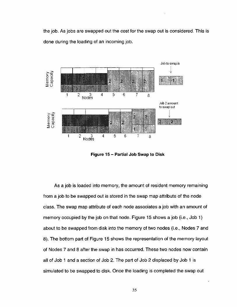
Figure 15 - Partial Job Swap to Disk

As a job is loaded into memory, the amount of resident memory remaining

from a job to be swapped out is stored in the swap map attribute of the node

class. The swap map attribute of each node associates a job with an amount of

memory occupied by the job on that node. Figure 15 shows a job (i.e., Job 1)

about to be swapped from disk into the memory of two nodes (i.e., Nodes 7 and

8). The bottom part of Figure 15 shows the representation of the memory layout

of Nodes 7 and 8 after the swap in has occurred. These two nodes now contain

all of Job 1 and a section of Job 2. The part of Job 2 displaced by Job 1 is

simulated to be swapped to disk. Once the loading is completed the swap out

3 5

overhead is calculated. This is done by using the swap out amounts contained in

the swap out maps of the nodes allocated to the job that was swapped to disk.

The maximum amount of memory in any node swapped to disk is divided by the

transfer rate of the node. This gives the time taken to swap that amount of

memory to disk. This time is then added to the remaining running time for the job

swapped out. This simulates the time taken to swap out one job to accommodate

an incoming job. The maximum time is used since once the job has been

preempted to swap out one section of the swapped job, no running progress can

be made by that job. The code for this process is contained in the "loadJob"

method detailed in Appendix A.

The swap out map used to calculate the swap costs as applied to each

preempted job is passed in as a parameter to this method and then used to

determine the time to add by a simple loop detailed in Figure 16. This loop adds

the swap out cost to the remaining running time of each swapped job.

/ / A d j u s t each swapped out job f o r swap out cost f o r ( I t e r a t o r i t e r = swapOutMap.entrySetQ . i t e r a t o r ( ) ; i t e r , h a s N e x t ( ) ; ) {

Map.Entry en t r y = (Map.Entry) i t e r . n e x t Q ; Dob j ob = (Dob) e n t r y . g e t K e y ( ) ;

i n t timeToAdd = ( ( I n t e g e r ) e n t r y , g e t V a l u e ( ) ) . i n t V a l u e ( ) ;

job.setRemainingRunt ime(job.getRemainingRunt ime() + t imeToAdd);

}

Figure 16 - Adjustment according to Swap out Cost

5.4 Memory Modelling

Each job created using the Lublin-Feitelson model is assigned a random

percentage of a node's total memory capacity. This is done by using a memory

36

model object. Each object contains a memory model listing that specifies a range

of possible percentages or shares of the nodes total memory a job will consume.

This assignment is based on the length of the job. Jobs of differing lengths

typically utilize different memory profiles, longer jobs typically being wider (i.e.,

using more nodes) and using a greater share of memory per node than shorter

jobs. The implementation of this supports a reconfigurable memory model. As

each job is created it is assigned a memory requirement randomly over a

distribution of values. The possible memory distribution models used are as

shown in Figure 17.

p r i v a t e doub le t ] defaul tModel = { 0 . 3 , 0 . 3 , 0 . 3 , 0 . 4 , 0 . 4 , 0 . 5 , 0 . 5 , 0 . 6 , 1 . 0 , 1 . 8 } ; p r i v a t e doub le f ] highMemModel = { 0 . 6 , 0 . 6 , 0 . 7 , 0 . 7 , 0 . 8 , 0 . 8 , 0 . 9 , 0 . 9 , 1 . 0 , 1 . 0 } ; p r i v a t e doub le f ] lowMemModel = { 0 . 1 , 0 . 1 , 0 . 2 , 0 . 2 , 0 . 2 , 0 . 3 , 0 . 3 , 0 . 4 , 0 . 4 , 0 . 5 } ; p r i v a t e doub le f ] veryHighMemModel = { 0 . 7 , 0 . 7 , 0 . 8 , 0 . 8 , 0 . 9 , 0 . 9 , 1 . 0 , 1 . 0 , 1 . 0 , 1 . 0 } ; p r i v a t e doub le f ] veryLowMemModel = { 0 . 1 , 0 . 1 , 0 . 1 , 0 . 2 , 0 . 2 , 0 . 2 , 0 . 3 , 0 . 3 , 0 . 3 , 0 . 4 } ;

Figure 17 - Memory Models

Each value in the vector represents a percentage of the nodes total

memory that the job will occupy. For example, as a job is created, a memory

model is assigned based on its type (short, medium, or large). Each job type is

assigned a vector from the ones described in Figure 17. Then a random number

between 1 and 10 is used to determine the value selected from the vector. This

value selected from the vector is assigned as the percentage of a node's total

memory is that required by that job. For example, in the simulation suppose

medium jobs are configured to utilize the high memory model vector (i.e.,

highMemModel in Figure 17). When a medium job is created from the synthetic

37

workload a random number between 1 and 10 is chosen. Suppose the number

chosen is 8. The eighth number in the high memory model vector is 0.9. This

means that the medium job created will be assigned 90% of the memory capacity

of a node as the job's memory requirement. The random assignment creates a

uniform distribution over the values in the vector. This means that if medium jobs

are assigned the high memory model then 20% of medium jobs will require 60%

of a nodes memory, 20% will require 70%, 20% will require 80%, 20% will require

90% and 20% will require 100%. If the medium jobs are assigned the default

memory model (i.e., defaultModel in Figure 17) then 30% of the medium jobs will

require 30% of a nodes memory, 20% will require 40%, 20% will require 50% ,

10% will require 60% and 20% will require 100%.

Figure 18 gives an indication of the percentage of jobs that have various

memory requirements in the LANL-CM5 workload trace. The LANL-CM5

workload trace is from a 1024 node cluster where each node has a memory

capacity of 32 MB. It shows that a low percentage of jobs use more than half the

memory capacity of the nodes. Approximately 50% of the jobs in the workload

require less than 5000 kB of memory, or 15% of the total capacity. This

distribution can be simulated by assignment of the very low memory model

vector (i.e., veryLowMemModel in Figure 17) to short job types when using the

synthetic (i.e., Lublin-Feitelson) workload model. Approximately 64% of jobs

generated by the synthetic workload model are of type short. Assignment of

memory model vectors with higher percentages to long and medium job types

produces a distribution curve similar in shape to the LANL-CM5 model.

38

Percent Si -Of Wrldo.id ; ;; „

35 -

\

This raph diows the job men ion,- requirement * in the IAN1.CM 5 workload trace plotted in.ii n st i peroeul of the total number of jobs in the workload. Hie memory cajvicitv of ncxies .in this duster is 32 MB. It show'Atlrar most jobs (50%i only require less than 5000 kJ> of me trior,". It also shows that a relatively small percentage of jobs require more tlvau half of the foia.1 memory c ap aritv of t he duster node s. Only a tew jobs in tlie entire workload require the entire memorv capadty

i&ooo issso sccso ssoss aoses ssseo

lob Memorv Requirements (kilobytes)

Figure 18 - LANL-CM5 Workload Memory Requirements

The assignment of a percentage of a nodes total memory is suitable for

the purposes of this analysis. This is because we are examining the effects of the

algorithm on reducing overhead given the assumption that our job workload is

such that jobs may or may not fully occupy the memory available in a node. The

importance is in evaluation of the allocation algorithm in the context of jobs which

require different amounts of a nodes total memory. This type of design and

implementation was chosen in order to support reconfigurability of the memory

model. This supports analysis of more accurate workloads and memory profiles.

The code for the memory model implementation is detailed in Appendix D.

39

5.5 Fitting Allocator Classes

The implementation for sorting nodes by memory space based on worst fit

and best fit were implemented as extensions of a super class "NodeAllocator".

This design was chosen to provide a standard interface for development of

different types of node allocators based on differing criteria. The current

implementation of the simulator supports three variations:

• Best-Fit Allocator

• Worst-Fit Allocator

• First-Fit Allocator

In the simulation implementation each allocator implements a standard interface.

This interface takes the job to be allocated and a list of nodes on which to

allocate the job according to the algorithm contained in the allocation classes.

This allows for analysis of differing allocation methods at the different stages in

the overall allocation algorithm. The specific details for each allocation algorithm

are described in Appendix C.

40

6. TESTS

6.1 Experimental Setup

This section describes the general experimental setup used in the

evaluation of the algorithm in reducing overhead. The experiments were

performed using the previously mentioned Lublin-Feitelson model for the creation

of synthetic workloads. In the evaluations 10 random workload schedules were

utilized, with all workload schedules showing utilization between 80% and 85%

during the tests. These workload schedules are lists of jobs, the jobs

characteristics, and the arrival time of each job to the simulator. For example, job

1 requires 10 nodes and arrives at time 100 seconds after start.

Actual workload traces were also utilized from the Feitelson workload

archive [5], these being SDSC-BLUE and LANL-CM5 workloads. In determining

the memory characteristic for each real workload trace the memory requirements

in the SDSC-BLUE trace do not consume the total memory per node in any

combination of three jobs. In fact the SDSC-BLUE trace does not contain

memory information except the amount requested by the running process. The

memory per processing node of the SDSC-BLUE trace is 512 MB per node. No

combination of three jobs in the trace exceeds one third of the available memory

and therefore when this trace is used we assign memory to these jobs according

to the randomized model. In the LANL-CM5 trace, the jobs in the workload do in

some cases consume the total memory of the node. When using this workload

trace the actual percentages of the total memory per node as requested by the

job are used.

41

The workload parameters for the synthetic and real workloads are

described in Table 1. Runtime estimates, which are used for classification (short,

medium, long) are assumed to be accurate. While this is not the case with most

job scheduling, there is research indicating jobs may be profiled to have an

indication of the runtime [3]. In our case we assume all jobs to have perfect

estimation

The type of job determines which slice the jobs are allocated to run in. The

amount of runtime each job gets is based on the method presented in [6] [7] and

does not change as a result of the modified node allocation algorithm. Jobs are

also classified according to width (narrow, medium, wide); however, this is

unimportant in the evaluation of overhead produced for a global schedule and

workload. The percentage of jobs in each category is shown in Table 2, along

with the percentage of the total workload each job type represents. The transfer

rate per node was set at 1 % of the total node memory per second can be

transferred. This is consistent with the speed and transfer rates of modern cluster

computer systems which typically can contain 16 GB of memory per node.

Typical disk transfer rates approach an average read/write speed of 100 MB/s [4]

and so the simulated transfer time is slightly faster than that based on nodes

having 16 GB of memory with a 100 MB/s transfer rate (16 384 MB /100 MB/s =

163 seconds. We currently model 100 seconds for complete transfer of

memory). The previous versions of the scheduler specified a global slice switch

overhead of 60 seconds which would be similar to an average case in the

42

updated simulation where all jobs may not completely fit into memory but only

part of the memory would need to be swapped out at any interval [22].

Parameter Value

Number of jobs in workload 10000 Classification of short jobs Runtime < 10 minutes Classification of medium jobs 10 minutes < Runtime < 3 hours Classification of long jobs 3 hours < Runtime Backfilling Heuristic Conservative - Non-Type Slice

Backfilling Enabled Interval 24 Intervals per day (1 per hour)

Table 1 - Scheduling Parameters

Lublin-Feitelson SDSC BLUE LANLCM5 Machine Size 128 1152 1024 Percentage of Short 64% 73.75% 61.4% Jobs Percentage of 19.5% 17.7% 34.2% Medium Jobs Percentage of Long Jobs

16.5% 8.5% 4.3%

Workload 0.5% 1.0% 2.5% Percentage for Short Jobs Workload 26.0% 15.0 % 40.7% Percentage for Medium Jobs Workload 73.5% 84.0% 56.8% Percentage for Long Jobs

Table 2 - Workload Characteristics

Several test cases were constructed and the resulting overhead incurred

was measured in each case over each of the 10 random workload schedules.

43

The test cases compared the use of the previous intelligent node allocation

method as detailed in [6] [7] and the separate "first free" nodes available method

against different variations of the memory aware allocation algorithm presented

here. The first free nodes available method simply is the case where a job is

allocated on nodes not currently being used in the running slice without

consideration as to memory usage or swap costs.

The previously described intelligent node allocation algorithm used in [6] [7]

seeks to reduce the number of jobs of differing types (short, medium, long) which

share the same nodes. It does not take into consideration memory usage or

swap costs in the determination, only commonly used nodes and can be seen as

a very basic approximation of the modified allocation algorithm presented here.

The new allocation algorithm is then varied by using different fitting methods (i.e.,

best-fit and worst-fit) in the two stages of the algorithm. This is done to find the

best configuration of the algorithm. Each configuration is also tested against

varying memory models to examine how different memory characteristics of jobs

impact the new allocation algorithm and how it compares to the other allocation

methods.

Overhead time is defined as the total time spent either loading or unloading

a job to and from the memory of a node. Modifications to the cluster simulation

allow for accounting of the overhead of each job individually regardless of the

scheduler object used. Relative response time is calculated using a bound on the

runtime for short jobs. This prevents short jobs from having a very large relative

response time when the actual response time may be very short compared to

44

longer jobs in the schedule. For example, a job needing 1 seconds of runtime

may wait 5 minutes (i.e., 300 seconds) to run and then finish. That job's relative

response time would then be 300 which is a very high value when compared to

the actual response time. This is appropriate since from a typical users point of

view the responsiveness of a job should be relative to the computation performed

(i.e., runtime). However, it is also reasonable to expect users to wait a short time

for a job to finish even if the ratio of response time to runtime is very high, as in

the example above. The relative response time for jobs is calculated as shown in

Figure 19.

if Runtime > Bound

if Runtime < Bound & Response Time > Bound

if Response Time <= Bound

Figure 19 - Relative Response Time Calculation

The reduction in overhead and any improvement in relative response time are

calculated as shown in Figure 20.

J •Response Time / Runtime

Relative Response Time = ^ Response T ime/ Bound

•1

45

Overhead Reduction = 1 - Overhead"] ime ot Allocation Algorithm

Overhead Time otT est Algorithm

Relative Response Time Improvement = 1 - Relative Response Time of Allocation Algorithm

Relative Response Time of Test Algorithm

Figure 20 - Improvement Calculation Equations

6.2 Results and Interpretation

Tables 4 - 9 show the overhead reduction of the presented algorithm as

compared to the basic "first free" allocation and the intelligent node allocation

algorithm from [6] [7]. Tables 4 - 7 also show the relative response time

improvement of the allocation algorithm as compared to the same previously

used methods. Relative response time improvement was shown to examine the

impact of overhead reduction on improving the overall schedule. The results from

the synthetic environment represent the averages from the individual test runs. In

all cases the relative response times were similar to that of the previous versions

of the scheduler. The graph shows the relative improvement of the presented

heuristic over the two alternative heuristics. Tables 4, 5, 6 and 7 detail the

percentage improvement of the new job allocation algorithm over the previous

"first-free" and intelligent node allocation algorithms. Each table represents a

different configuration of the new algorithm where the best-fit and worst-fit

algorithms were utilized in either the first stage or second stage respectively.

Figure 20 shows the percentage improvement over 5 different memory model

46

assignments as detailed in Table 3. Each memory-model assignment represents

which memory-model vector as shown in Figure 17 that was assigned to which

job type. In Figure 20, the improvement over the first free allocation method is

indicated by the "FF" designation for each memory model assignment. The

improvement over the intelligent node allocation method is indicated by the "AL"

designation for each memory model assignment. All the results in Tables 4 -7

and Figure 21 are the average of the improvements observed over all ten

generated synthetic workloads. Tables 8 and 9 show the improvements of the

new allocation algorithm over the actual workload traces LANL-CM5 and SDSC-

BLUE.

Memory Model Assignment Job Size to Model Vector

MM1 Long = highMemModel Medium = defaultModel Short = lowMemModel

MM2 Long = lowMemModel Medium = defaultModel Short = highMemModel

MM3 Long = veryHighMemModel Medium = defaultModel Short = veryLowMemModel

MM4 Long = veryLowMemModel Medium = defaultModel Short = veryHighMemModel

MM5 Long = defaultModel Medium = defaultModel Short = defaultModel

Table 3 - Memory Model Assignment

47

Test Case ID

Test Case Description (Synthetic Workload)

Memory Model Used for Job Type

Overhead Reduction over first free allocation

Overhead Reduction over basic Node Allocation

Relative Response Improvement over first free

Relative Response Improvement over basic Allocation

1 Best Fit - First Stage Worst Fit -Second Stage

MM1 6.04% 2.91%

L 2.31% M 0.01% S0.01% A 1.01%

L 3.9% M 0.1% S0.01% A 1.42%

2

Best Fit - First Stage Worst Fit -Second Stage

MM2 3.95% 2.62%

L 2.21% M 0.02% S 0.04% A 1.07%

L 1.9% M 0.1% S 0.30% A 0.09%

3


MM3 2.31% 0.23%

L 1.31% M 0.01% S 0.21% A 1.91%

L 0.92% M 0.00% S0.11% A 0.72%

4


MM4 2.75% 0.81%

L 2.01% M 0.61% S0.01% A 1.00%

L 0.94% M 0.1% S0.01% A 0.56%

5


MM5 13.84% s thesL

L 3.31% M 0.01% S0.01% A 1.01%

L 2.9% M 0.01% S0.01% A 0.98%

Table 4 - Synthetic Load Test Results - Best-Fit/Worst-Fit

Test Case ID







6

Best Fit - First Stage Best Fit -Second Stage

MM1 6.02% 2.89%

L 2.37% M 0.42% S0.01% A 1.01%

L 0.54% MO.13% S0.01% A 0.45%

7


MM2 1.73% 0.42%

L 1.91% M 0.41% S 0.14% A 1.01%

L 0.85% M 0.18% S 0.14% A 0.45%

8


MM3 3.74% 1.41%

L 1.32% M 0.72% S 0.41% A 1.81%

L 3.9% M 0.63% S 0.435% A 1.42%

9


MM4 2.71% 0.77%

L 2.31% M 1.51% S 0.71% A 1.04%

L 2.01% M 0.31% S 0.31% A 0.92%

10


MM5 8.02 % 1.65%

HD&DDDD M 2.01% S 1.41% A 1.71%

L 3.01 % M 1.17% S 1.21% A 1.42%

Table 5 - Synthetic Load Test Results - Best-Fit/Best-Fit

48

Test Case ID







11

Worst Fit - First Stage Worst Fit -Second Stage

MM1 2.84% 0.79%

L 1.41% M 0.01% S 0.01% A 1.11%

L 0.09% M 0.01% S0.01% A 1.01%

12


MM2 1.24% 0.31%

L 1.21% M 0.02% S 0.70% A 1.17%

L 0.08% M 0.01% S 0.70% A 0.64%

13


MM3 2.22% 1.18% L 1.33% M 0.01% S 0.23% A 1.93%

L 0.95% M 0.00% S0.14% A 0.75%

14


MM4 5.96% 3.96%

L 1.91% M 0.58% S 0.01% A 1.01%

L 0.90% M 0.11% S 0.01% A 0.54%

15


MM5 4.82 % 0.11% L 1.30% M 0.98% S0.01% A 1.01%

L 0.90% M 0.01% S0.01% A 0.98%

Table 6 - Synthetic Load Test Results - Worst-Fit/Worst-Fit

Test Case ID







16 Worst Fit - First Stage Best Fit -Second Stage

MM1 2.37% 0.32% L 2.12% M 0.42% S 1.61% A 1.01%

L 1.54% M 0.13% S 0.01% A 0.45%


MM2 0.68% 0.11%

L 1.78% M 0.71% S 0.14% A 1.02%

L 0.85% M 0.48% S 0.14% A 0.46%


MM3 5.45% 3.08%

L 2.32% M 0.72% S 0.41% A 1.81%

L 1.91% M 0.63% S 0.29% A 1.42%

19

Worst Fit - First Stage Best Fit -Second Stage

MM4 2.59% 0.66%

L 1.31% M 1.51% S 0.71% A 1.04%

L 1.01% M 0.31% S 0.31% A 0.92%

20

Worst Fit - First Stage Best Fit -Second Stage

MM5 8.94 % 2.52%

L 1.31% M 1.41% S 1.21% A 1.61%

L 0.81% M 1.17% S 1.11% A 1.40%

Table 7 Synthetic Load Test Results - Worst-Fit/Best-Fit

49

FF AL FF AL FF AL FF AL FF AL

• Best/Worst • Best/Best • Worst/Worst • Worst/Best

Figure 21 - Synthetic Load Comparative Results

Test Case ID




1 Best Fit - First Stage Worst Fit - Second Stage

5.50 % 0.25%

2 Best Fit - First Stage Best Fit - Second Stage

4.45% 0.80%

3

Worst Fit - First Stage Worst Fit - Second Stage

7.70% 2.58%

4

Worst Fit - First Stage Best Fit - Second Stage

6.16% 0.95%

Table 8 - SDSC-BLUE Workload Test Results

50

Test Case ID Test Case Description (Synthetic Workload)



1 Best Fit - First Stage Worst Fit - Second Stage

5.45% 1.99 %

2 Best Fit - First Stage Best Fit - Second Stage

8.62% 5.27%

3 Worst Fit - First Stage Worst Fit - Second Stage

6.59% 3.17%

4 Worst Fit - First Stage Best Fit - Second Stage

3.99% 0.47%

Table 9 - LANL-CM5 Workload Test Results

6.3 Overall Test Results

From the test runs we can see that in all cases the presented algorithm

reduces the amount of overhead incurred in the running system. The algorithm

seems especially effective if the memory required by jobs does not trend

according to job size. That is, the amount of memory required by a job does not

indicate the amount of nodes or degree of parallelism required by the job. The

general trend seems to be that inclusion of the "best-fit" fitting technique in either

the first or second stages of the allocation heuristic improves the reduction of

overhead. There was no real significant improvement in relative response times

observed over the previous allocation methods. This is due to the simulation

attributing a small percentage the total time to overhead as compared with the

total running time of the simulation. Small jobs in particular, for the most part,

51

either finish within the slice in which they first receive runtime or experience very

little additional overhead as a result. For medium and large jobs the overhead

modelled was insignificant to make an appreciable difference in improvement

toward relative response times. Additionally, in some individual test runs the

relative response times were worse for certain job types even though the amount

of accumulated overhead was less. The average relative response times over all

test runs remained relatively unchanged as shown in Tables 4 - 7 . Though not

shown in Tables 8 and 9, the relative response times also remained relatively

unchanged. This is most likely due to the fact that different orders of jobs present

different opportunities for backfilling. If a job cannot fit on nodes it incurs no

overhead. The job just simply waits in a queue. This adds further evidence that if

overhead does not represent a significant amount of the total processing time

then it is of minor concern as compared to backfilling choices made during the

scheduling process. Even though response times may behave slightly differently

than relative response times, no significant response time improvement was

observed.

In general the technique improves the reduction of overhead over the

original intelligent node allocation method as well as over the "first nodes free"

type of allocation. There still is no guarantee that this method provides the best

packing of jobs given the other concern of fairness implied with the initial first-

come, first-serve consideration of the SCOJO-Pect scheduler.

52

7. CONCLUSIONS AND FUTURE WORK

The test results show that the presented algorithm is effective in reducing

the overhead by amounts ranging from 0.11% - 7.13 % over the previous

intelligent node selection heuristic. The presented algorithm is most effective

where the job runtime does not indicate the memory requirements for that job.

However, even in this context the overhead compared to the actual work or

processing done on the nodes still accounts only for about 1.5% of the total

processing time in the workload models. This amount is lower than previous

simulations and models since overhead is calculated on a per job basis and only

when jobs preempt. Previous simulation models imposed higher levels of

overhead in the 5-10% range [6] [7]. This was due to modelling the preemption

overhead globally across all jobs instead of individually as in the updated

simulator. As the overhead costs for preemption increase, the performance of the

algorithm in reducing incurred preemption cost would likely become more

effective. Increasing overhead costs could be caused by larger memory

reguirements for running jobs or slower transfer rates from memory to disk. In the

future, if job memory requirements grow faster than memory to disk transfer rates

then overhead costs will increase.

The improvement is only notable when compared against the overhead

from a very basic allocation method that does not consider memory swap times.

In the case that overhead times become a significant factor in the processing of

parallel jobs, a better method may be toward the design of a purpose built

system. In this case the jobs to be run and the hardware would each be designed

53

to complement the other. That is parallel jobs and tasks are designed from the

outset to run in a particular environment with efficiency under constraints that

guarantee achieving the desired optimality criteria. An example of this would be a

system designed such that all jobs have a specific degree of parallelism (e.g., all

jobs require 16 nodes). The hardware would then be designed to support these

specific job types to achieve maximum use of the processing nodes.

The modelling of the performance of overhead characteristics also depends

on the speed of the hardware for which the overhead is incurred. An advance in

hardware and increased memory sizes may make overhead costs a non-factor.

On the other hand if there is advancement in the amount of data to be processed

along with increasingly accurate estimates of runtime then techniques that

consider overhead costs may be of value.

Future work continuing from this point could include expanding the job

modelling to include jobs that can relocate to differing nodes as well as jobs that

can alter their degree of parallelism upon preemption. These processes would

also incur overhead that may need to be managed and a determination made as

to whether any change is necessary. Another future direction could include

analysis of patterns which may appear in the schedule that indicate future

opportunities for advantageous backfilling. However, even this would be limited

by each set of hardware and job types having a unique advantageous pattern

types which would need to be modelled in advance of any sort of optimization.

54

Appendix A Node.java

package hpcSimulation;

import hpcSimulation. jobs.Job; import j a v a . u t i l . A r r a y L i s t j import java.ut i l .HashMap; import j a v a . u t i l . I t e r a t o r ; import j a v a . u t i l . M a p ;

/ * * *

* @author Bryan Esbaugh * /

public class Node {

public State ge tS ta te ( ) { return s ta te ;

}

public void se tSta te (Sta te s ta te ) { t h i s . s t a t e = s ta te ;

}

* @return the jobMemorySwapMap * /

public HashMap<Integer, Integer> getDobMemorySwapMap() { return jobMemorySwapMap;

}

public s t a t i c enum State {

FREE, LOADING, RUNNING }; pr iva te s t a t i c i n t memorySize = 400; / / S i z e of memory in the node p r i va te s t a t i c i n t t ransferRate = 4 ; / / T h e speed in MB/s of t r a n s f e r

between disc and node memory\ p r i va te ArrayList<Dob> jobsInMemory; p r i va te i n t nodelD = 0; p r i va te i n t currentlyRunningDobID = -1 ; p r i va te boolean ava i l ab le = t r u e ; p r i va te State s ta te ; p r i va te HashMapcInteger, Integer> jobMemorySwapMap; / * *

* Constructor fo r a node object *

* * /

public Node() {

55

jobsInMemory = new ArrayList<Job>() ;

jobMemorySwapMap = new HashMap<Integer, I n t e g e r > ( ) ;

s ta te = State.FREE;

} / * *

* Loads jobs in to the memory of the node. This happens at the end of * the loading so tha t in the simulation t h i s method would be ca l led * when the job has completed loading. *

* (Sparam j The job the load in to memory * (Sparam swapOutMap The swap out map used to ca lcu la te the time cost of

swapping out jobs. * (Slreturn I f the job was successful ly loaded return t r u e , else return

f a l s e * /

public boolean loadDob(Dob j , HashMap<Job, Integer> swapOutMap) {

i f ( this.getFreeMemory() >= j.getMemoryReq()) { th is . jobsInMemory.add( j ) ; this.getDobMemorySwapMap() .put( j .get ld() , j .getMemoryReq()) j

return t r u e ; } else {

/ /Rout ine to handle loading job to displace memory, while (this.getFreeMemory() < j .getMemoryReq()) {

/ / F i n d the amount of memory remaining from displaced job. i n t memRemaining = 0j i n t memFree = this.getFreeMemory() j / / F r e e memory before

removing job

Dob job = this. jobsInMemory.remove(0); / / D o n ' t remove job from

map.

i f ( this.getFreeMemory() >= j.getMemoryReqQ) {

memRemaining = j.getMemoryReq() - memFreej / /Remaining amount of job memory th is . jobsInMemory.add( j ) ;

/ / F i n d the time to swap out the job and that tha t time to the remaining runtime to simulate the swap out cost.

i n t timeForSwapOut = memRemaining / Node.getTransferRate() ;

i f (!swapOutMap.containsKey(job)) { swapOutMap.put(job, timeForSwapOut);

} e lse i f (swapOutMap.get( job) . intValue() < timeForSwapOut) {

56

swapOutMap.put(job, timeForSwapOut); }

this.getDobMemorySwapMap() .put( job.getld() , memRemaining); this.getDobMemorySwapMapQ.put( j .get ld() ,

j .getMemoryReq()); return t r u e ;

} e lse {

this.getDobMemorySwapMapQ.put( job.getId() , 0 ) ; }

} i f ( I th is . jobs InMemory .conta ins ( j ) ) {

throw new RuntimeException("Dob not sucessful ly loaded"); } return f a l s e ;

}

} !**

* This checks t o see i f a c e r t a i n job is loaded in to the memory of the node

*

* @param j - Dob to check * @return t rue i f job is in memory, or f a l s e otherwise * /

public boolean jobInMemory(Dob j ) {

f o r (Dob jn : this. jobsInMemory) { i f ( j n . g e t l d ( ) == j . g e t l d ( ) ) {

re turn t r u e ; }

}

return f a l s e ; } / * *

* Removes a job from the memory of the node *

* @param j Dob to be removed * ^return Returns t rue i f job removed, f a l s e otherwise * /

public boolean removeDobFromMem(Dob j ) {

i f ( th is . jobs InMemory .conta ins ( j ) ) { th is . jobsInMemory.remove( j ) ; this.getDobMemorySwapMapQ.remove(j .getld()); return t r u e ;

} e lse {

return f a l s e ;

57

}

}

public s t a t i c i n t getMemorySize() { return memorySize;

}

public s t a t i c void setMemorySize(int memorySize) { Node.memorySize = memorySize;

}

public s t a t i c i n t getTransferRate( ) { return t ransferRate ;

}

public s t a t i c void setTransferRate( int t ransferRate ) { Node.transferRate = t ransferRate ;

} / * *

* Quick f i x fo r keeping the remaining runtimes consistent with * those in the Preemptive scheduler preemption queues. * *

* (Sparam job * /

public void setNodeDobRuntimeRemaining(Dob job) {

f o r (Dob j : this.jobsInMemory) {

i f ( j . e q u a l s ( j o b ) ) { j .setRemainingRuntime(job.getRemainingRuntime());

} }

}

protected i n t getFreeMemory() { i n t memory = Node.memorySize;

f o r (Dob j : this.jobsInMemory) {

memory -= j .getMemoryReqQ; }

return memory; }

public i n t getNodelDQ { return nodelD;

}

public void setNodeID(int nodelD) { th is .nodelD = nodelD;

}

58

public i n t getCurrentlyRunningDob() { re turn currentlyRunningDobID;

}

public void setCurrentlyRunningDob(Dob currentlyRunningDob) {

i f (currentlyRunningDob.getldQ == - 1 ) { throw new RuntimeException("Trying to s t a r t a negative Dob");

} i f ( this. joblnMemory(currentlyRunningDob)) {

this.currentlyRunningDobID = current lyRunningDob.get Id( ) ; th is .setState(State .RUNNING); t h i s . s e t A v a i l a b l e ( f a l s e ) ;

} e lse { this.currentlyRunningDobID = current lyRunningDob.get ldQ; th is .setState(State .LOADING); t h i s . s e t A v a i l a b l e ( f a l s e ) ; / / throw new RuntimeException("Trying to s t a r t job not loaded in

Memory"); }

}

public void setCurrentlyRunningDob(int currentlyRunningDob) { i f (currentlyRunningDob == - 1 ) {

throw new RuntimeException("Trying to s t a r t a negative Dob"); } i f ( this. jobsInMemory.contains(currentlyRunningDob)) {

this.currentlyRunningDobID = currentlyRunningDob; th is .setState(State .RUNNING); t h i s . s e t A v a i l a b l e ( f a l s e ) ;

> else { this.currentlyRunningDobID = currentlyRunningDob; th is .setState(State .LOADING); t h i s . s e t A v a i l a b l e ( f a l s e ) ;

} }

public void stopCurrentlyRunningDob() {

this.currentlyRunningDobID = - 1 ; t h i s . a v a i l a b l e = t r u e ; th is .se tS ta te (S ta te .FREE) ;

} / * *

* Returns t rue i f the node already has a job running on i t or i f i t has been marked

* as unavai lable fo r the current scheduling phase. *

* (Sreturn * /

public boolean i s A v a i l a b l e ( ) { i f ( this.currentlyRunningDobID != - 1 ) {

59

re turn f a l s e ; } else {

re turn t h i s . a v a i l a b l e ; }

} / * *

* Sets whether the node is ava i l ab le or not. Does not al low a node with a job current ly

* running to be set to a v a i l a b l e . *

* @param a - t rue or f a l s e i f the node i s ava i l ab le * /

public void setAvai lable(boolean a) { i f ( th is .current lyRunningJobID != - 1 ) {

t h i s . a v a i l a b l e = f a l s e ; } else {

t h i s . a v a i l a b l e = a; >

}

ArrayList<Dob> getDobsInMemory() {

return this. jobsInMemory;

} }

60

Appendix B Cluster.allocateJob()

* Memory A l loca t ion heur is t i c which a l locates jobs to nodes based on memory pressure

*

* @param j s - The job to a l l o c a t e to resources. * /

pr iva te i n t [ ] allocateDob(Dob j s ) {

BestF i tA l locator bfa = new B e s t F i t A l l o c a t o r ( ) ; WorstFi tAl locator wfa = new Wors tF i tA l loca to r ( ) ;

ArrayList<Node> freeNodes = new ArrayList<Node>(); / / L i s t of f r e e nodes with ava i l ab le memory

ArrayList<Node> nodeList = new ArrayList<Node>(); / / L i s t of nodes

i n t [ ] ind ic ies = new i n t [ j s . g e t N o p t ( ) ] ;

i n t [ ] totalMemoryUsedlnNode = new int [ th is .Simulat ionParameters.getNODES() ] ; / / The number of nodes in the c lus te r

ArrayList<Dob> preemptedDobs = ((PreemptionScheduler) scheduler) .getAl lPreemptDobsQ;

f o r ( i n t i = 0; i < getRunningQueueQ.size() ; i++) { preemptedDobs.add(getRunningQueue ( ) . g e t D o b ( i ) ) ;

}

/ / G e t the memory used in t o t a l fo r each node. This would mean tha t the node, f o r comparison

/ / a g a i n s t what i s in memory at the time of the schedul ing /a l locat ion phase.

fo r (Dob j : preemptedDobs) {

fo r ( i n t i : j . ge tNode Ids ( ) ) { totalMemoryUsedInNode[i] += j .getMemoryReqQ;

} }

/ / G e t the l i s t of nodes with immediately ava i l ab le memory fo r the job / / T h i s l i s t should be reduced by the t o t a l amount of memory used by

jobs, / / S i n c e i t makes no sense to t r y to assign jobs to nodes tha t do not

have enough memory to hold / / a l l cur rent ly assigned jobs, f o r (Node n : th is .nodes) {

i f ((n.getFreeMemoryQ >= js.getMemoryReq()) && n . i s A v a i l a b l e Q ) { i f (Node.getMemorySize() -

totalMemoryUsedlnNode[n.getNodelDQ] >= js.getMemoryReqQ) { freeNodes.add(n);

61

} } / /End I f

} / /End For

/ /Check i f we have enough nodes with enough a v a i l a b l e memory / / f o r the job we wish to a l l o c a t e / /The node a l loca t ion i s switchable between BestFi t and WorstFit

i f ( f reeNodes.s ize( ) >= j s . g e t N o p t Q ) { ind ic ies = b f a . a l l o c a t e ( j s , freeNodes);

} / /End i f e lse {

/ / I f we have not found enough nodes with a v a i l a b l e memory we t r y to a l l o c a t e to nodes

/ /w i thou t enough ava i lab le memory in rank order of increasing time remaining u n t i l the

/ / j o b s f ree memory resources.

for (Node n : th is .nodes) { i f (totalMemoryUsedInNode[n.getNodeID()] < js.getMemoryReq()

&& n . i s A v a i l a b l e ( ) ) { / /node doesn't have enough f ree memory nodeList .add(n);

} / / end i f } / / e n d fo r

sortByTimeUnti lAHDobsFit(nodeList j j s ) ;

i n t index = 0; fo r (index = 0; index < nodeL is t . s i zeQ && index < j s . g e t N o p t Q ;

index++) { ind ic ies f index] = nodeLis t .get ( index) .getNodeID( ) ;

}

/ / I f the number of nodes in the node l i s t was i n s i f f i c i e n t to a l l o c a t e

/ / t h e job, then we add nodes to the l i s t of ind ic ies such tha t the job

//may be f u l l y a l located .

i n t [ ] sublndicies = n u l l ; i f (nodeL is t . s i zeQ < j s . g e t N o p t Q ) {

ArrayList<Node> extraNodeList = new ArrayList<Node>();

f o r (Node n : th is .nodes) { i f ( ( I n o d e L i s t . c o n t a i n s ( n ) ) && ( n . i s A v a i l a b l e ( ) ) ) {

extraNodeList .add(n); }

}

62

sublndicies = w f a . a l l o c a t e ( j s , extraNodeList ) ;

i n t sublndex = 0j whi le (index < j s . g e t N o p t Q ) {

ind ic ies [ index ] = sublndicies[sublndex]; index++; sublndex++;

} }

} / / end else

return i n d i c i e s ;

}

63

Appendix C Fitting Algorithms

C.I Best Fit

The best fit algorithm is used for on-line bin packing where the goal is to

place items in "bins" as they arrive such that the number of bins used is a

minimum [12]. As applied to our overhead minimization methods, we utilize this

general idea to assign jobs to nodes, which have enough available memory to

contain all jobs currently assigned, where the amount of available memory on the

node is minimized. The effect of this is to group jobs together on already utilized

nodes in order to leave room for other more memory intensive jobs. The

expected effect would be that narrow jobs (i.e., jobs requiring a small number of

nodes) having less memory requirements would group together on nodes leaving

room for wider jobs (i.e., jobs requiring large numbers of nodes) elsewhere in the

cluster. The implementation of the best fit job allocator is in Figure 22.

64

package hpcSimulation.nodeAllocation;

import hpcSimulation.NodeFreeMemoryComparator; import hpcSimulation.jobs.Dob; import java.util.ArrayList; import java.util.Collections;

* Best Fit Node Allocator for HPC Cluster Dobs *

* Packs jobs according to "Best Fit Algorithm" , that is attempts to pack * jobs onto nodes such that the job fits onto nodes with the least amount * of free space available such that jobs still fit in the available memory. *

* (Sauthor Bryan Esbaugh */

public class BestFitAllocator extends NodeAllocator {

^Override

public int[] allocate(Dob js, ArrayList<hpcSimulation.Node> freeNodes) {

int[] indicies = new int[js.getNopt()]; NodeFreeMemoryComparator comparator = new NodeFreeMemoryComparator(); Collections.sort(freeNodes, comparator);

for (int i = 0; i < js.getNoptQ && i < freeNodes.size(); i++) {

indicies[i] = freeNodes.get(i).getNodeID(); } return indicies;

} }

Figure 22 - Best Fit Allocator Implementation

C.ll Worst Fit

The worst fit heuristic attempts to put any newly arrived object into any open

bin where there is the most extra space. In this case the free space in each bin is

keep at a maximum and objects are spread across all bins. In the allocation

method, this means that jobs will be allocated to nodes where after allocation

there will be a maximum amount of free space. This means that instead of

65

grouping jobs together, jobs are spread across empty nodes. The implementation

is shown in Figure 23.

package hpcSimulation.nodeAllocation;

import hpcSimulation.Node; import hpcSimulation.NodeFreeMemoryComparator; import hpcSimulation.jobs.3ob; import java.util.ArrayList; import java.util.Collections; /**

* Implements "Worst Fit" Alogorithm, this algorithm attempts to place job on * nodes with the most available space. *

* (Sauthor Bryan Esbaugh */

public class WorstFitAllocator extends NodeAllocator{

^Override public int[] allocate(3ob js, ArrayList<Node> freeNodes) {

int[] indicies = new int[js.getNopt()]; NodeFreeMemoryComparator comparator = new NodeFreeMemoryComparator(); Collections.sort(freeNodes, comparator);

int sizeOfFreeNodes = freeNodes.size();

for ( in t i = 0; i < js.getNoptQ && i < freeNodes.size(); i++) {

indicies[i] = freeNodes.get(sizeOfFreeNodes - i -1).getNodelDQ;

} return indicies;

} >

Figure 23 - Worst Fit Allocator Implementation

C.lll First Fit

First fit simply maintains a list of current bins, or nodes in our case, and

upon arrival of a job, puts that object in the first bin in which it fits [12]. This

method for job allocation to nodes is not utilized for the purposes of

66

experimentation in this paper, but is supported by the updated scheduler. The

implementation is shown in Figure 24.

package hpcSimulation.nodeAllocation; import hpcSimulation.Node; import hpcSimulation.jobs.Dob; import java.util.ArrayList;

/public class FirstFitAllocator extends NodeAllocator{

^Override public int[] allocate(Dob js, ArrayList<Node> freeNodes) {

int[] indicies = new int[js.getNopt()]; for (int i = 0; i < js.getNopt() && i < freeNodes.size(); i++) {

indicies[i] = freeNodes.get(i).getNodeID(); } return indicies;

}

Figure 24 - First Fit Allocator Implementation

67

Appendix D MemoryModel.java

package hpcSimulation;

import edu.Cornell . lassp.houle.RngPack.Ranmar; import j a v a . i o . * ; import j a v a . u t i l . * ;

/ * *

* Class representing the memory model to be used in the assignment of memory requirements

* to jobs. *

* @author Bryan Esbaugh

public class MemoryModel {

p r i va te i n t seed; Random gen; p r iva te i n t maximumMemory;

p r iva te double[] defaultModel = { 1 . 0 , 0 . 3 , 0 . 3 , 0 . 4 , 0 . 5 , 0 . 4 , 0 . 3 , 0 . 6 , 1 . 0 , 0 . 5 } ;

p r iva te double[] highMemModel = { 0 . 6 , 0 . 6 , 0 . 7 , 0 . 7 , 0 . 8 , 0 . 8 , 0 . 9 , 0 . 9 , 1 . 0 , 1 . 0 } ;

p r i va te doublef] lowMemModel = { 0 . 1 , 0 . 1 , 0 . 2 , 0 . 2 , 0 . 2 , 0 . 3 , 0 . 3 , 0 . 4 , 0 . 4 , 0 . 5 } ;

p r iva te doublef] veryHighMemModel = { 0 . 7 , 0 . 7 , 0 . 8 , 0 . 8 , 0 . 9 , 0 . 9 , 1 . 0 , 1 . 0 , 1 . 0 , 1 . 0 } ;

p r iva te doublef] veryLowMemModel = { 0 . 1 , 0 . 1 , 0 . 1 , 0 . 2 , 0 . 2 , 0 . 2 , 0 . 3 , 0 . 3 , 0 . 3 , 0 . 4 } ;

p r iva te double usedModelf] = defaultModel;

MemoryModel(int SEED) { th is .seed = SEED; gen = new Random(seed); this.maximumMemory = Node.getMemorySize();

} / * *

* Gets the randomly generated memory requirement f o r a job. *

* @return * /

public i n t getMemoryRequirement(){ i n t memory =0; gen.next Int (usedModel . length) ; memory = ( i n t ) (this.maximumMemory * usedModel [gen.next In t (10) ] ) ; re turn memory;

public void setSeed(

i n t seed) {

68

th is .seed = seed; }

public i n t getMaximumMemory() { return maximumMemory;

} / * *

* Set the maximum memory a v a i l a b l e to *

* @param MaximumMemory * /

public void setMaximumMemory(int MaximumMemory) { this.maximumMemory = MaximumMemory;

> * Set the d i s t r i b u t i o n model for the job memory requirement *

* @param model

public void setDistr ibut ionModel(double [ ] model){

this.usedModel = model;

}

i n t getMemoryRequirement(int nopt) {

/ /Conf igurab le memory model changable based on job width.

i f (nopt < 13){ usedModel = th is .de fau l tMode l ;

> else i f (nopt < 65){ usedModel = th is .de fau l tMode l ;

} else{

usedModel = th is .de fau l tMode l ; }

i n t memory =0; gen.next Int (usedModel . length) ; memory = ( i n t ) (this.maximumMemory * usedModel [gen.next Int (10) ] ) ; return memory;

} }

69

Appendix E Job Scheduling Visualization

An additional feature added to the Cluster Simulator was the addition of a

job schedule visualization engine. Figure 25 shows the main interface and

display panel for the visualization engine. The main design of this feature

consists of a number of objects that are created and displayed on a visualization

panel. Initially space on the visualization panel along the y axis is divided into

horizontal bands which represent the nodes of the cluster. The x-axis along the

visualization panel is used to represent time. As each event in the simulation

occurs, a determination is made as to whether this can be visually represented

on the panel. If so, then an object representing the event overtime is drawn.

In the case of jobs on nodes at each job finish or preemption, a rectangle

filling part of the band is displayed in the x-y space representing that jobs

occupancy overtime on that node. Each job is given a distinct colour based on

the jobs characteristics (i.e. estimated length). Other events, such as slice

switches, or preemptions, are represented by vertical lines across all the node

bands placed along the x -axis corresponding to the time at which the event

occurred. As the simulation progresses, the user is able to see jobs progressing

and a very high level view of how the jobs are laid out on the simulated cluster

resources. One of the problems with this approach is to be able to define a set,

or the assignment, of colours such that patterns can be seen at a glance.

Additionally, if the job mix consists of a wide range in the length of jobs it is very

difficult to discern patterns as the user must zoom in very close to see shorter

70

jobs and zoom out to see longer jobs in the same context. Colouring of the jobs

based on more global criteria such as increasing wait times may give better

indications as to patterns in the job mix.

JobGeneratiwu ;lub&n-Fe&ebonW... * SeedVatas'. • Scheduler' f*empti« -» • | ietTrace ] Nodes: -liQ

Number rf Jobs : 1000 ! Zoom f ) • Trace: none > Collect 5*ats j Print Queues rJ Find Daly Averages

Figure 25 - Cluster Simulator Visualization

71

Bibliography

[1] Brucker, P. Scheduling Algorithms. Berlin Heidelberg, pages 107-108. Springer 2006

[2] Canetti, R., Irani, S. "Bounding the Power of Preemption in Randomized Scheduling." Proceedings of the Twenty-Seventh Annual ACM Symposium on theory of Computing (Las Vegas, Nevada, United States, May 29 - June 01, 1995), pages 606-615. Symposium on Theory of Computing '95. ACM, New York, NY,

[3] Carrington, L., Wolter, N., Snavely, A., Lee, C.B., "Applying an Automated Framework to Produce Accurate Blind Performance Predictions of Full-Scale HPC applications." Proc. DoD Users Group Conference. IEEE, 2004.

[4] Dertouzos, M.L., Mok, A.K. "Multiprocessor On-Line Scheduling of Hard-Real-Time Tasks." IEEE Transactions in Software Engineering, vol 15, no. 12, pages 1497-1506, 1989

[5] Dobrin, R., Fohler, G. "Reducing the Number of Preemptions in Fixed Priority Scheduling," Proceedings of the 16th Euromicro Conference on Real-Time Systems June 30 - July 02, pages 144-152, 2004

[6] Esbaugh, B., Sodan, A., "Coarse-grain Time Slicing with Resource-Share Control in Parallel-Job Scheduling." Proc. High Performance Computing and Communication (HPCC). Houston, Lecture Notes in Computer Science 4782: Springer, September 2007

[7] Esbaugh, B., Sodan, A., "Preemption and Share Control in Parallel Job Scheduling." Grid Middleware and Services, Challenges and Solutions, pages 121-135, Springer, June 2008

[8] Feitelson, D. "Feitelson Workload Archive," The Hebrew University of Jerusalem. 01 Dec. 1998. 11 May 2010 <http://www.cs.huji.ac.il/ labs/parallel/workload/logs. html>

[9] Feitelson, D. "Memory Usage in the LANL CM-5 workload," Lecture Notes in Computer Science vo\. 1291 pages 78-94, 1997

[10] Jette, M.A. "Performance Characteristics of Gang Scheduling in Multiprogrammed Environments," Proceeding of the 1997 ACM/IEEE Conference on Supercomputing. San Jose, CA, Nov. 15-21, 1997 pages 1-12, Supercomputing '97. ACM, New York, NY

72

http://www.cs.huji.ac.il/%e2%80%a8labs/parallel/workload/logs.%20html

http://www.cs.huji.ac.il/%e2%80%a8labs/parallel/workload/logs.%20html

[11] Jung, K.J., Park, C. "A Technique to Reduce Preemption Overhead in Real-Time Multiprocessor Task Scheduling." Lecture Notes in Computer Science vol. 3740 pages 566-579, 2005

[12] Kenyon, C. "Best-Fit Bin-Packing with Random Order." Proceedings of the Seventh Annual ACM-SIAM Symposium on Discrete Algorithms, Atlanta, Georgia, United States, January 28 - 30, 1996, pages 359-364, Symposium on Discrete Algorithms. Society for Industrial and Applied Mathematics, Philadelphia, PA, 1996

[13] Kettimuthu, R., Subramani, V., Srinivasan, S., Gopalsamy, T., Panda, D.K., Sadayappan, P. "Selective Preemption Strategies for Parallel Job Scheduling," International Journal of High Performance Computing and Networking, vol 3 Issue 2/3, pages 122-152 , Nov 2005

[14] Klonowska, K., Lundberg, L., H. Lennerstad, H. "The Maximum Gain of Increasing the Number of Preemptions in Multiprocessor Scheduling." Acta Informatica vol. 46 number 4 pages 285-295, 2009

[15] Klusacek, D., Rudova, H., Baraglia, R., Pasquali, M., Capannini, G. "Comparison of Multi-Criteria Scheduling Techniques," Grid Computing, Achievements and Prospects, pages 173-184, July 11, 2008

[16] Lo, V., Mache, J. "Job Scheduling for Prime Time vs. Non-prime Time," Proceedings of the IEEE international Conference on Cluster Computing, pages 43-54, Sept 23-26, 2002.

[17] Lublin, U., Feitelson, D. "The Workload on Parallel Supercomputers -Modelling the Characteristics of Rigid jobs." Journal of Parallel and Distributed Computing, vol 63, no. 11, pages 1105-1122, November 2003.

[18] Murphy, D. "The (new) Fastest Hard Drive Ever," MaximumPC. 21 April 2008. 11 May 2010 <http://www.maximumpc.com/article/the new fastest hard drive ever>

[19] Ousterhout, J.K. "Scheduling Techniques for Concurrent Systems," Proceedings of the 3rd International Conference on Distributed Computer Systems, pages 22-30, 1982

[20] Pfeiffer, W., Boisseau, J., Chukkapalli, G. "Expanding the Horizon for Academic Scientific Computing," San Diego Supercomputer Center. May 11, 2010 <http://www.sdsc.edU/pub/envision/v16.1/bluehorizon.html >

[21] Pruhs, K.; Torng, E.; Sgall, J., "Online Scheduling." Handbook of Scheduling: Algorithms, Models, and Performance Analysis, ed Joseph Y.T. Leung, chapter 15, pages 15-1 - 15-41, CRC Press, 2004

73

http://www.maximumpc.com/article/the%20new%20fastest%20hard%20drive%20ever

http://www.sdsc.edU/pub/envision/v16.1/bluehorizon.html

[22] Sodan, A.C. "Autonomic Share Allocation and Bounded Prediction of Response Times in Parallel Job Scheduling for Grids," IEEE International Symposium Network Computing and Applications, pages 307-314. 2008 Seventh IEEE International Symposium on Network Computing and Applications, 2008

[23] Sodan, A.C. "Loosely Coordinated Coscheduling in the Context of Other Approaches for Dynamic Job Scheduling: A Survey: Research Articles." Concurrency and Computation: Practice & Experience, vol 17, Issue 15 pages 1725-1781, Dec 2005

74

VITA AUCTORIS

Bryan Esbaugh was born in Halifax, Nova Scotia. He obtained a B.A. in Political Science in 1996. From there he obtained a B.Sc. Honours in Computer Science - Software Engineering from the University of Windsor in 2007. He is currently a candidate for a Masters Degree in Computer Science and hopes to graduate in

the summer of 2010.

75

Coarse-grain time sharing with advantageous overhead ...

Documents

Transcript of Coarse-grain time sharing with advantageous overhead ...