CLIP4: Hybrid inductive machine learning algorithm that generates inequality rules
47
CLIP4: Hybrid inductive machine learning algorithm that generates inequality rules Krzysztof J. Cios a,c,d,e, * , Lukasz A. Kurgan b a Department of Computer Science and Engineering, University of Colorado at Denver, Campus Box 109, P.O. Box 173364, Denver, CO 80217-3364, USA b Department of Electrical and Computer Engineering, University of Alberta, Edmonton, AB T6G 2V4, Canada c Department of Computer Science, University of Colorado at Boulder, Boulder, CO 80309, USA d University of Colorado Health Sciences Center, Denver, CO 80262, USA e 4cData, Golden, CO 80401, USA Received 8 May 2002; accepted 17 March 2003 Abstract The paper describes a hybrid inductive machine learning algorithm called CLIP4. The algorithm first partitions data into subsets using a tree structure and then generates production rules only from subsets stored at the leaf nodes. The unique feature of the algorithm is generation of rules that involve inequalities. The algorithm works with the data that have large number of examples and attributes, can cope with noisy data, and can use numerical, nominal, continuous, and missing-value attributes. The algorithm’s flexibility and efficiency are shown on several well-known benchmarking data sets, and the results are compared with other machine learning algorithms. The benchmarking results in each instance show the CLIP4’s accuracy, CPU time, and rule complexity. CLIP4 has built-in features like tree pruning, methods for partitioning the data (for data with large number of examples and attributes, and for data containing noise), data- independent mechanism for dealing with missing values, genetic operators to improve accuracy on small data, and the discretization schemes. CLIP4 generates model of data that consists of well-generalized rules, and ranks attributes and selectors that can be used for feature selection. Ó 2003 Elsevier Inc. All rights reserved. * Corresponding author. Address: Department of Computer Science and Engineering, University of Colorado at Denver, Campus Box 109, P.O. Box 173364, Denver, CO 80217-3364, USA. Tel.: +1-303-556-4314/4083; fax: +1-303-556-8369. E-mail addresses: [email protected] (K.J. Cios), [email protected] (L.A. Kurgan). 0020-0255/$ - see front matter Ó 2003 Elsevier Inc. All rights reserved. doi:10.1016/j.ins.2003.03.015 Information Sciences 163 (2004) 37–83 www.elsevier.com/locate/ins
-
Upload
independent -
Category
Documents
-
view
3 -
download
0
Transcript of CLIP4: Hybrid inductive machine learning algorithm that generates inequality rules

Information Sciences 163 (2004) 37–83
www.elsevier.com/locate/ins
CLIP4: Hybrid inductive machine learningalgorithm that generates inequality rules
Krzysztof J. Cios a,c,d,e,*, Lukasz A. Kurgan b
a Department of Computer Science and Engineering, University of Colorado at Denver,
Campus Box 109, P.O. Box 173364, Denver, CO 80217-3364, USAb Department of Electrical and Computer Engineering, University of Alberta,
Edmonton, AB T6G 2V4, Canadac Department of Computer Science, University of Colorado at Boulder, Boulder, CO 80309, USA
d University of Colorado Health Sciences Center, Denver, CO 80262, USAe 4cData, Golden, CO 80401, USA
Received 8 May 2002; accepted 17 March 2003
Abstract
The paper describes a hybrid inductive machine learning algorithm called CLIP4.
The algorithm first partitions data into subsets using a tree structure and then generates
production rules only from subsets stored at the leaf nodes. The unique feature of the
algorithm is generation of rules that involve inequalities. The algorithm works with the
data that have large number of examples and attributes, can cope with noisy data, and
can use numerical, nominal, continuous, and missing-value attributes. The algorithm’s
flexibility and efficiency are shown on several well-known benchmarking data sets, and
the results are compared with other machine learning algorithms. The benchmarking
results in each instance show the CLIP4’s accuracy, CPU time, and rule complexity.
CLIP4 has built-in features like tree pruning, methods for partitioning the data (for data
with large number of examples and attributes, and for data containing noise), data-
independent mechanism for dealing with missing values, genetic operators to improve
accuracy on small data, and the discretization schemes. CLIP4 generates model of data
that consists of well-generalized rules, and ranks attributes and selectors that can be
used for feature selection.
� 2003 Elsevier Inc. All rights reserved.
* Corresponding author. Address: Department of Computer Science and Engineering, University
of Colorado at Denver, Campus Box 109, P.O. Box 173364, Denver, CO 80217-3364, USA. Tel.:
+1-303-556-4314/4083; fax: +1-303-556-8369.
E-mail addresses: [email protected] (K.J. Cios), [email protected] (L.A. Kurgan).
0020-0255/$ - see front matter � 2003 Elsevier Inc. All rights reserved.
doi:10.1016/j.ins.2003.03.015
38 K.J. Cios, L.A. Kurgan / Information Sciences 163 (2004) 37–83
Keywords: CLIP4; Inductive machine learning; Inequality rules; Feature selection;
Feature ranking; Selector ranking
1. Introduction
The paper describes a new supervised inductive machine learning (ML)
algorithm called CLIP4. It generates model of the data that consists of pro-
duction rules, plus feature and feature-value importance ranking that is cal-
culated from the generated rules.
It is the only algorithm to our knowledge that generates inequality rules,
which makes it complementary to many existing machine learning algorithms.
Below, we list major goals which any supervised inductive learning system
should possess to assure its wide applicability:
• Accurate classification––the generated rules need to accurately classify new
unseen during rule generation examples, even in the presence of noise.
• Simple rules––the generated rules should be compact. Less complex rules are
easier to comprehend. They also lead to more accurate classification than
complex rules [33].
• Efficient rule generation––the algorithm must scale up well to generate rules
for large data.• Flexibility––the algorithm should work on wide range of problems. In case
of supervised ML, learning problems are characterized by the number of
examples (large that usually covers the state space, or small that usually cov-
ers only part of the state space), the number of attributes, the type of attri-
butes (discrete numerical, discrete nominal, continuous), the presence of
noise, and the missing value attributes.
The first three goals are typical in design of ML algorithms [17]. CLIP4satisfies these three goals, as well as the last goal of flexibility. The four goals
are indispensable features of any state-of-the-art ML algorithm.
The paper first overviews current approaches to supervised inductive ML
and provides outline of the CLIP4 algorithm, along with an illustrative
example. Next, benchmarking results are presented, its performance is com-
pared with other ML algorithms, and significance of the results is dis-
cussed.
1.1. CLIP4 and other related algorithms
The first CLIP algorithm, the CLILP2 (Cover Learning using Integer LinearProgramming) was developed in 1995 [12,13]. The algorithm was later

K.J. Cios, L.A. Kurgan / Information Sciences 163 (2004) 37–83 39
improved as CLIP3 [14,16]. The described here CLIP4 algorithm incorporates
major changes and improvements from its predecessors that result in more
accurate, efficient, and flexible algorithm.
CLIP4 is a hybrid algorithm that combines ideas of two families of inductiveML algorithms, namely the rule algorithms and the decision tree algorithms. It
uses rule generation schema from AQ algorithms [38,56,59]. It also uses the tree
growing technique that divides training data into subsets at each level of the
tree, and pruning [4,74].
The main difference between CLIP4 and the two families of algorithms is
extensive use of the set covering (SC) problem. The SC constitutes core ope
ration performed many times by CLIP4. It is used to select the most dis-
criminating features, grow new branches of the tree, select data subsets fromwhich the algorithm generates the least overlapping and the most general
rules, and finally to generate rules from the leaf-subsets using a back-pro-
jection technique (described later). Solving the SC problem is also one of
operations used in the LAD algorithm [5]. Another algorithm that is a hybrid
of rule algorithms and decision tree algorithms is the CN2 algorithm [17,18]
which is a modification of the AQ algorithm that uses search strategy and
entropy measure in a way similar to the one used in decision tree algo-
rithms.The main feature distinguishing CLIP4 from other ML algorithms is that it
generates production rules that involve inequalities, which makes it comple-
mentary to algorithms that generate rules that involve equalities, such as AQ
algorithms, decision trees ([72]), and a MetaSqueezer system ([49–51]). This
results in generating small number of compact rules for domains where attri-
butes have large number of discrete values, and when majority of them are
correlated with the target class. In contrast, generation of rules involving
equalities for such domains would results in generating dozens of very complexrules.
2. The CLIP4 algorithm
2.1. Introduction
Learning concept descriptions, in the form of if-then rules or decision
trees, is the most popular form of machine learning [7]. Any supervised
inductive learning algorithm infers classification rules from training exam-
ples divided into two categories: positive and negative. The generated
rules should describe the positive examples and none of the negative exam-ples.

40 K.J. Cios, L.A. Kurgan / Information Sciences 163 (2004) 37–83
2.2. The algorithm
2.2.1. Solution of the set covering problem
Several key operations performed by CLIP4 are modeled and solved by theSC problem. To make it more efficient we developed a new method for solving
the SC problem.
The SC problem [1,28] is a simplified version of the integer programming
(IP) model. The IP model is used for optimization of a function, subject to a
large number of constraints [64]. In the IP model several simplifications are
made to obtain the SC problem: the function that is subject of optimization has
all coefficients set to one, their variables are binary, i.e. xi ¼ f0; 1g, constraintfunction coefficients are binary, and all constraint functions are greater orequal to one. The SC problem is NP-hard [26,37] and thus only approximate
solution can be found.
An example SC problem and its matrix representation are shown in Fig. 1.
The solution to the SC problem can be found using the constraint coeffi-
cients matrix, which we call the BINary matrix. Its columns correspond to
variables (attributes) of the optimized function. Rows correspond to function
constrains (examples). The solution is obtained by selecting minimal number of
matrix columns in such a way that for every row there will be at least onematrix cell with the value of 1 for the selected columns. All the rows for which
there is value of 1 in the matrix cell, in a particular column, are assumed to be
‘‘covered’’ by this column. The solution consists of a binary vector composed
of the selected columns.
For CLIP4 we need to have a fast solution to the SC problem since it is used
many times over, that significantly effects computation time. In the CLIP3
algorithm a simple greedy algorithm was used to obtain the SC solution
[14,15]. The new method, used in the CLIP4 algorithm, seeks solution of theSC problem in terms of selecting minimal number of columns, which also have
the smallest total number of 1’s. This is solved by minimizing the number of 1’s
Fig. 1. Simplified SC problem and its solution shown in standard and matrix forms.

K.J. Cios, L.A. Kurgan / Information Sciences 163 (2004) 37–83 41
that overlap among the columns and within the same row. The new solution of
the SC problem results in improved accuracy and generalization ability of
CLIP4-generated rules, see Section 4.4.
The pseudo-code of the CLIP4’s method for solving the SC problem fol-lows:
Given: BINary matrix, Initialize: Remove all empty rows from the BINary
matrix; if the matrix has no 1’s then return error.
1. Select active rows that have the minimum number of 1’s––min-rows.
2. Select columns that have the maximum number of 1’s within the min-rows––
max-columns.
3. Within max-columns find columns that have the maximum number of 1’s in
all active rows––max-max-columns, if there is more than one max-max-col-
umn go to 4, otherwise go to 5.
4. Within max-max-columns find the first column that has the lowest numberof 1’s in the inactive rows.
5. Add the selected column to the solution.
6. Mark the inactive rows, if all the rows are inactive then terminate; otherwise
go to 1.
where: the active row is the row that is not covered by the partial solution,
and the inactive row is the row that is already covered by the partial solution.
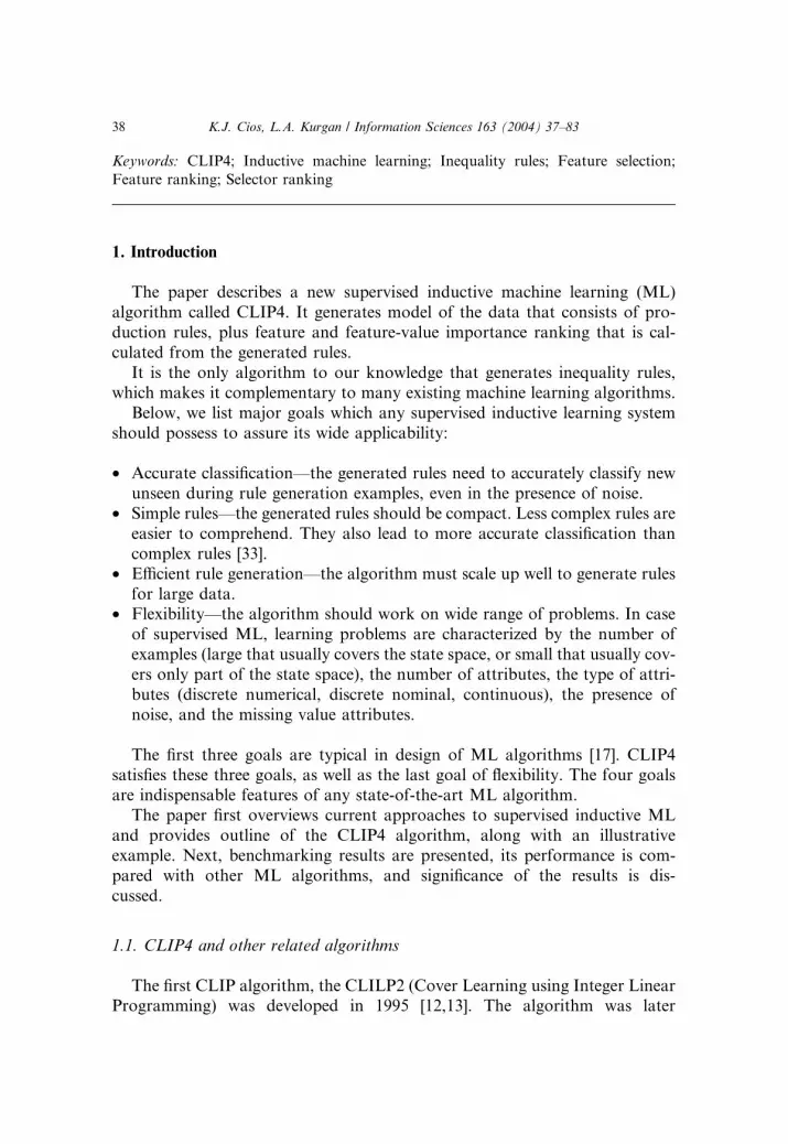
The solution for the example using the new method is shown in Fig. 2a. Theexample is as the one shown in Fig. 1, except that some matrix rows (con-
strains) are repeated. The solution consists of the second and fourth columns,
with no overlapping 1’s in the same rows. For comparison, Fig. 2b shows the
result obtained by the method used in CLIP3; there are two solutions
depending on how the choice of columns is performed: Solution one has one 1
overlapping in the first row; solution two has two 1’s overlapping in the first
and third rows.
2.2.2. The CLIP4 details
To describe the algorithm we first introduce some notations. Let us denotethe set of all training examples by S. The sets of the positive examples, SP, andthe negative examples, SN, must satisfy these properties: SP [ SN ¼ S,SP \ SN ¼ £, SN 6¼ £, and SP 6¼ £. The positive examples are those that de-
scribe the class for which we currently generate rules, while the negative
examples are all remaining examples. Examples are described by a set of Kattribute-value pairs [57,58]: e ¼ ^K
j¼1½aj#vj] where aj denotes jth attribute with
value vj 2 dj, # is a relation (¼ , <, �, 6 , etc.), where K is the number of
attributes. An example e consists of set of selectors sj ¼ ½aj ¼ vj�. The CLIP4algorithm generates rules in the form of:
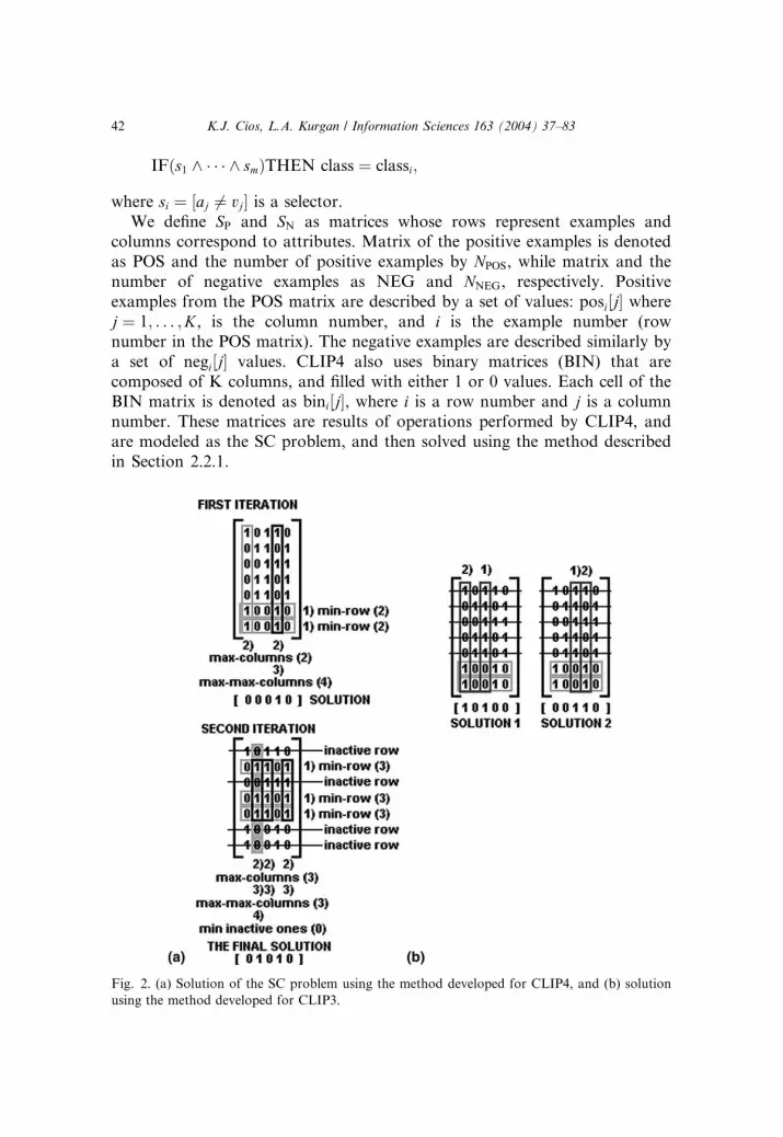
Fig. 2
using t
42 K.J. Cios, L.A. Kurgan / Information Sciences 163 (2004) 37–83
IFðs1 ^ � � � ^ smÞTHEN class ¼ classi;
where si ¼ ½aj 6¼ vj� is a selector.
We define SP and SN as matrices whose rows represent examples andcolumns correspond to attributes. Matrix of the positive examples is denoted
as POS and the number of positive examples by NPOS, while matrix and the
number of negative examples as NEG and NNEG, respectively. Positive
examples from the POS matrix are described by a set of values: posi½j� wherej ¼ 1; . . . ;K, is the column number, and i is the example number (row
number in the POS matrix). The negative examples are described similarly by
a set of negi½j� values. CLIP4 also uses binary matrices (BIN) that are
composed of K columns, and filled with either 1 or 0 values. Each cell of theBIN matrix is denoted as bini½j�, where i is a row number and j is a column
number. These matrices are results of operations performed by CLIP4, and
are modeled as the SC problem, and then solved using the method described
in Section 2.2.1.
. (a) Solution of the SC problem using the method developed for CLIP4, and (b) solution
he method developed for CLIP3.

K.J. Cios, L.A. Kurgan / Information Sciences 163 (2004) 37–83 43
The low-level pseudocode of CLIP4 is shown in Fig. 3. Below we explain the
main phases of the algorithm.
Fig. 3. The low-level pseudo code of CLIP4.

44 K.J. Cios, L.A. Kurgan / Information Sciences 163 (2004) 37–83
Phase I explanation:
• General idea
The positive data is partitioned into subsets of similar data in a decision-treelike manner. Each node of the tree represents one data subset. Each level of the
tree is built using one negative example to find selectors that can distinguish
between all positive and this particular negative example. The selectors are
used to create new branches of the tree. During tree growing, pruning is used to
eliminate noise from the data, to avoid its excessive growth, and to reduce
execution time.
• Pseudo-code explanation (lines 2–23 in Fig. 3)
The tree, with nodes representing subsets of positive examples, is grown inthe top-down manner. At the ith tree level Ni subsets, represented by matrices
POSi;j (j ¼ 1; . . . ;Ni), are generated using Ni�1 subsets from the previous tree
level, and the single negative example negi. Each subset, represented by matrix
POSi;j (examples that constitute this matrix are denoted as posi;j), is trans-
formed into a BIN matrix of the size of the POSi;j matrix, using the negiexample, and then modeled and solved using the new SC method. The solution
is used to generate subsets for the next tree level, represented by POSiþ1;j
matrices.• Important features
The algorithm grows a virtual ‘‘tree’’. The ‘‘tree’’ at any iteration consists
of only one, the most recent tree level. In addition, the virtual tree is pruned
so that even the one level that is kept has at most a few nodes. This result in
high memory efficiency. The data splits are done by generating not just one
‘‘best’’ division, based on the ‘‘best’’ feature say in terms of the highest value
of information gain, but by a set of divisions based on any feature that
distinguishes between the positive and the one negative example. Thismechanism of partitioning the data assures generation of the (possibly) most
general rules.
Phase II explanation
• General idea
A set of best terminal subsets (tree leaves) is selected using two criteria. First,
large subsets are preferred over small ones since the rules generated from themcan be ‘‘stronger’’ and more general, while all accepted subsets (between them)
must cover the entire positive training data. Second, we want to use the
completeness criterion. To that end, we first perform a back-projection of one
of the selected positive data subsets using the entire negative data set, and then
we convert the resulting matrix into a binary matrix and solve it using the SC
method. The solution is used to generate a rule, and the process is repeated for
every selected positive data subset.

K.J. Cios, L.A. Kurgan / Information Sciences 163 (2004) 37–83 45
• Pseudo-code explanation (lines 24–41 in Fig. 3)
The NNNEGis the number of the tree leaves. The BIN is the binary matrix
used to select the minimal set of leafs that covers the entire positive data. Back-
projection results in a binary matrix BINi that has 1’s for the selectors that candistinguish between positive and negative examples. The back-projection
generates one matrix for every best terminal subset (POSNNEG;i). It is computed
from the NEG matrix, by setting a value from NEG to zero if the same value
appears in the corresponding column in the POSNNEG;i matrix, otherwise the
value if left unchanged. The ith rule is generated by solving the SC problem for
the BINi matrix and adding a selector for every 1 that is in any column indi-
cated by the solution.
• Important features
The rule generation technique generates a rule directly from two sets of data
(negative data and the selected subset of positive data). It does not require the
use of logic laws like in the AQ algorithms, or storing and traversing the entire
tree as done in decision tree algorithms, but only by simple comparison of
values between the two matrices. Thus, the only data structures required to
generate the rules are lists (vectors) and matrices.
Phase III explanation:
• General idea
A set of best rules is selected from all the generated rules. Rules that cover
the most positive examples are chosen, which promotes selection of general
rules. If there is a tie between ‘‘best rules’’ the shortest rule is chosen, i.e. the
rule that uses minimal number of selectors.
• Pseudo-code explanation (lines 42–55 in Fig. 3)
To find the number of examples covered by a rule, we instead findexamples that are not covered by the rule, and subtract them from the total
number of examples. This is done because the rules consist of selectors
involving inequalities. The variable called coversi keeps the number of posi-
tive examples that are covered by the ith rule. After a rule is accepted
the positive examples covered by it are removed from the POS matrix (line
53).
• Important features
In Phase III more than one rule can be generated. The rules are accepted inorder from the most general and strong, to the weakest. The heuristic used for
accepting multiple rules states that the next rule is accepted when it covers at
least half of the number of examples covered by the previously accepted rule,
and that it covers at least half of the number of positive examples that were not
covered by any rule so far. CLIP4 generates multiple strong rules in a single
sweep through the data. The thresholds used in the pseudo-code in Fig. 3 are
described in Section 3.1.5.

46 K.J. Cios, L.A. Kurgan / Information Sciences 163 (2004) 37–83
In what follows we estimate the complexity of the CLIP4 algorithm for
generation of rules for one class. Let us start with these notations:
• n is number of examples, and k is number of attributes;• Ni, and NNNEG
are small constants, which are controlled by algorithm’s
thresholds (see Section 3.1.5);
• NPOS þ NNEG ¼ n––number of examples. Thus OðNPOSÞ ¼ OðNNEGÞ ¼ OðnÞ;• length of the SOL vector is k;• size of all POS and NEG matrices is kOðnÞ;• we also require, and assume, that n � k
Before we estimate the complexity of CLIP4, we can estimate the complexityof several operations performed by the algorithm:
• Estimation of complexity for solving the SC problem. This operation is de-
noted in the code in Fig. 3 by calling the following function: SolveSCProb-
lem(. . .)Assumption: BIN matrix has size kOðnÞLines 1–4: kOðnÞ eachLines 5 and 6: Oð1Þ eachIn the worst case entire algorithm (lines 1–6) are executed OðkÞ times, thus
the total complexity is:
kOðnÞ �OðkÞ ¼ Oðk2nÞ
• Estimation of complexity for pruning performed by CLIP4. This operationis denoted in the code in Fig. 3 by calling the function: PruneMatrices(. . .)Assumption: goodness criterion is computed in OðkÞ time
STEP 1: OðNi logNiÞ �OðkÞ ¼ Oð1Þ �OðkÞ ¼ OðkÞ to select the best nodes
STEP 2: OðNiÞ �OðNiÞ �OðnÞ ¼ Oð1Þ �Oð1Þ �OðnÞ ¼ OðnÞ to remove redun-
dant matrices; note: we look at the entire rows
STEP 3: OðNiÞ �OðnÞ ¼ Oð1Þ �OðnÞ ¼ OðnÞ to remove small matrices (belowthresholds)
Thus, the total complexity is: OðkÞ þOðnÞ þOðnÞ ¼ OðnÞ• Estimation of complexity for the genetics operations performed by CLIP4.
This operation is denoted in the code in Fig. 3 by calling the following func-
tion: ApplyGeneticOperators(. . .)Assumption: only one iteration of genetic operations is performed in line 12
of the code in Fig. 3, goodness criterion is computed in OðkÞ time
STEP 1: OðNi logNiÞ �OðkÞ ¼ Oð1Þ �OðkÞ ¼ OðkÞ to rank the individualsSTEP 2: OðNiÞ ¼ Oð1Þ to select half of the individuals with the best fitness
values
STEP 3: Performing crossover has complexity OðkÞPerforming mutation has complexity OðkÞ

K.J. Cios, L.A. Kurgan / Information Sciences 163 (2004) 37–83 47
ðOðkÞ þOðkÞÞ �OðNiÞ ¼ OðkÞ �OðNiÞ ¼ OðkÞ �Oð1Þ ¼ OðkÞ to per-
form genetic operations for the half of individuals with the worst
fitness values
Thus, the total complexity is: OðkÞ þOð1Þ þOðkÞ ¼ OðkÞ
To estimate complexity of the entire algorithm we break the process into
estimation of the complexity for particular phases of the algorithm:
1. Complexity of Phase I (lines 1–23 from the code in Fig. 3)
Line 1: OðknÞ to create both POS and NEG
Line 2: OðnÞ and applies to lines 3–23Line 3: OðNiÞ ¼ Oð1Þ and applies to lines 4–10
Line 4: OðkÞ and applies to lines 5–9
Line 5: OðnÞ and applies to lines 6–9
Lines 6–9: Oð1ÞLine 10: Oðk2nÞLine 11: OðnÞLine 12: OðkÞLine 13: Oð1ÞLine 14: OðNiÞ ¼ Oð1Þ and applies to lines 15–20
Line 15: OðNiÞ ¼ Oð1ÞLine 16: OðkÞ and applies to lines 17–19
Line 17: Oð1ÞLine 18: OðnÞ and applies to line 19
Line 19 and 20: Oð1ÞLine 21: OðNiÞ ¼ Oð1Þ and applies to lines 22
Line 22: Oð1ÞLine 23: OðnÞ (see PruneMatrices(. . .), STEP 2)
Total complexity of Phase I is estimated as:
OðknÞ þOðnÞ � ½Oð1Þ � ½OðkÞ � ½OðnÞ � ½Oð1Þ þOð1Þ þOð1Þ þOð1Þ��
þOðk2nÞ� þOðnÞ þOðkÞ þOð1Þ þOð1Þ � ½Oð1Þ þOðkÞ � ½Oð1ÞþOðnÞ þOð1Þ� þOð1Þ� þOð1Þ �Oð1Þ þOðnÞ�
¼ OðknÞ þOðnÞ � ½Oð1Þ � ½OðkÞ �OðnÞ þOðkÞ �Oðk2nÞ� þOðnÞþOðkÞ þOð1Þ � ½OðkÞ �OðnÞ� þOðnÞ�
¼ OðknÞ þOðnÞ � ½OðknÞ þOðk3nÞ þOðnÞ þOðkÞ þOðknÞ þOðnÞ�
¼ OðknÞ þOðkn2Þ þOðk3n2Þ þOðn2Þ þOðknÞ þOðkn2Þ þOðn2Þ
¼ OðknÞ þOðkn2Þ þOðk3n2Þ þOðn2Þ þOðknÞ ¼ Oðk3n2Þ

48 K.J. Cios, L.A. Kurgan / Information Sciences 163 (2004) 37–83
2. Complexity of Phase II (lines 24–41 from the code in Fig. 3)
Line 24: kOðnÞLine 25: OðNNNEG
Þ ¼ Oð1Þ and applies to lines 26 and 27
Line 26: OðnÞ and applies to line 27Line 27: OðnÞLine 28: Oðk2nÞLine 29: OðNNNEG
Þ ¼ Oð1Þ and applies to lines 30–41
Line 30: kOðnÞLine 31: OðkÞLine 32: OðkÞ and applies to lines 33–35
Line 33: OðnÞ and applies to lines 34, and 35
Line 34: Oð1ÞLine 35: OðnÞLine 36: OðkÞ and applies to line 37
Line 37: OðnÞLine 38: Oðk2nÞLine 39: OðkÞ and applies to lines 40, and 41
Line 40: Oð1ÞLine 41: OðnÞTotal complexity of Phase II is estimated as:
kOðnÞ þOð1Þ � ½OðnÞ �OðnÞ� þOðnÞ þOðk2nÞ þOð1Þ� ½kOðnÞ þOðkÞ þOðkÞ � ½OðnÞ � ½Oð1Þ þOðnÞ���
þOðkÞ �OðnÞ þOðk2nÞ þOðkÞ � ½Oð1Þ þOðnÞ�¼ kOðnÞ þOðn2Þ þOðnÞ þOðk2nÞ þOð1Þ � ½kOðnÞ þOðkÞþOðknÞ �Oðkn2Þ� þOðknÞ þOðk2nÞ þOðkÞ þOðknÞ
¼ kOðnÞ þOðn2Þ þOðnÞ þOðk2nÞ þ kOðnÞ þOðkÞþOðknÞ �Oðkn2Þ þOðknÞ þOðk2nÞ þOðkÞ þOðknÞ ¼ Oðkn2Þ
3. Complexity of Phase III (lines 42–55 from the code in Fig. 3)
Line 42: Oð1ÞLine 43: OðNiÞ ¼ Oð1Þ and applies to lines 44–55
(max # of rules ¼ # of leaf nodes)
Line 44: Oð1Þ and applies to lines 45–50Line 45: Oð1ÞLine 46: OðnÞ and applies to lines 47–49
Line 47: OðkÞ and applies to lines 48, and 49
Line 48: OðkÞ and applies to line 49
Line 49: Oð1ÞLine 50: Oð1ÞLines 51–55: Oð1ÞTotal complexity of Phase III is estimated as:

K.J. Cios, L.A. Kurgan / Information Sciences 163 (2004) 37–83 49
Oð1Þ þOð1Þ � ½Oð1Þ � ½Oð1Þ þOðnÞ � ½OðkÞ � ½OðkÞ �Oð1Þ�� þOð1Þ� þOð1Þ�
¼ Oð1Þ þOð1Þ � ½Oð1Þ � ½Oð1Þ þOðk2nÞ þOðknÞ� þOð1Þ� þOð1Þ�¼ Oð1Þ þOð1Þ � ½Oð1Þ þOðk2nÞ þOðknÞ þOð1Þ� þOð1Þ¼ Oð1Þ þOð1Þ þOðk2nÞ þOðknÞ þOð1Þ þOð1Þ ¼ Oðk2nÞe complexity of the entire algorithm is estimated as a sum of complexities
Thfor each of the phases as:
Oðk3n2Þ þOðkn2Þ þOðk2nÞ ¼ Oðk3n2Þ
Since the number of the generated rules and classes are usually small constants,
the above complexity describes complexity of generating all the rules for the
entire multi-class data. Thus, we estimate that the expected running time of the
algorithm is Oðk3n2Þ. Additionally, since number of attributes k is also usuallya small constant, we can estimate that the expected running time of the algo-
rithm is Oðn2Þ.The CLIP4 algorithm satisfies all of the following inductive machine
learning conditions [36]:
• completeness––the set of classification rules describes all positive examples,
• consistency––the classification rule must describe none of the negative exam-
ples,• convergence––the classification rules are generated in a finite number of
steps.
Additional condition, which requires generation of rules that involve min-
imal number of selectors, is also satisfied by the CLIP4 algorithm; it is done in
Phase III of the algorithm.
In a nutshell, the CLIP4 algorithm is memory-efficient thanks to keeping
only one level of the tree, generates general, strong rules thanks to its mech-anism of data partitioning and strong heuristics for rules acceptance, and is fast
because of pruning and accepting multiple rules in one iteration. In addition, it
is robust to noisy and missing-value data, which is shown in the following
sections.
2.3. Example of a rule generation by the CLIP4 algorithm
This example illustrates the working of CLIP4. There are eight data
examples belonging to two classes (see Table 1). Three examples have miss-ing values, denoted by ‘‘�’’. Class 1 is the positive class, class 2 the negative
class.

Table 1
Data for the example
Ex. # F1 F2 F3 F4 Class
1 1 2 3 * 1
2 1 3 1 2 1
3 * 3 2 5 1
4 3 3 2 2 1
5 1 1 1 3 1
6 3 1 2 5 2
7 1 2 2 4 2
8 2 1 * 3 2
50 K.J. Cios, L.A. Kurgan / Information Sciences 163 (2004) 37–83
The (a) low-level and (b) high-level illustration of CLIP4 rule generation.
RULE 1: If F 1 6¼ 3 and F 1 6¼ 2 and F 3 6¼ 2 then class 1
RULE 2: If F 2 6¼ 2 and F 2 6¼ 1 then class 1
The first rule covers examples 1, 2 and 5, while the second covers examples 2,
3 and 4. Between them they cover all positive examples, including those with
Fig. 4. The (a) low-level and (b) high-level example of rule generation by CLIP4.

K.J. Cios, L.A. Kurgan / Information Sciences 163 (2004) 37–83 51
missing values and none of the negative examples. The rules overlap since both
cover the second example.
The high-level view of the same example is shown in Fig. 4b. It shows how
CLIP4 performs tree generation, data partitioning, and rule generation.
3. Characteristics of the CLIP4 algorithm
CLIP4 retains the general structure of CLIP3 but it incorporates these newadditions:
• the new algorithm for solving the SC problem that results in more accurate
and general rules,
• handling of missing-values, continuous and nominal attributes,
• new tree-pruning technique that results in shorter execution time,
• application of genetic operators to improve accuracy of the algorithm for
small difficult data,• attribute and selector importance ranking.
3.1. General characteristics
3.1.1. Handling missing values
Missing-value data are typical, with often only some of the attributes having
missing values. Thus, at the level of a single example it is desirable to use all the
attributes that have values and omit from computations only the attributeswith missing values.
In case of the CLIP4 algorithm, no examples with missing values are dis-
carded, neither missing values are filled with some computed values. The
algorithm takes advantage of all available values in the example and ignores
missing values during rule generation.
The attributes with missing values influence the first two phases of the
algorithm. They are omitted from being processed by filling the corresponding
cell in the BIN matrix with 0 when the new branch of the tree in phase I isgenerated, and when the backprojection in phase II is performed (see Fig. 3).
The example in Fig. 4 shows how rules are generated from examples with
missing values. The mechanism for dealing with missing attribute values
implemented in CLIP4 assures that they are not used in the generated rules,
and at the same time all complete attribute values, even for the example that
has some missing attributes, are used during rule generation.
The advantage of CLIP4’s mechanism of dealing with missing values is that
the user can simply supply the data to the algorithm and obtain its modelwithout the need of using statistical methods to analyze the data with missing

52 K.J. Cios, L.A. Kurgan / Information Sciences 163 (2004) 37–83
values, assuming that the remaining (complete) part of the data is sufficient to
infer the model.
3.1.2. Handling of nominal attributes and generation of rules for multi-class data
CLIP4 handles nominal data by automatic front-end encoding into
numerical values. The generated rules are independent of the encoding scheme
since the algorithm does not calculate distances, nor does it apply any metric
during rule generation; instead it uses the SC problem that is independent of
actual values of the attributes. For multi-class data CLIP4 generates separate
set of rules for every class, each time generating rules that describe the currently
chosen (positive) class.
3.1.3. Handling of continuous attributes
A machine learning algorithm can deal with continuous values in two ways:
• It can process continuous attributes itself.
• It can perform front-end discretization. This approach is taken by algo-
rithms that handle only numerical or nominal data, like AQ algorithms
[17,18] or the CN2 algorithm [38,59].
Discretization research shows that some ML algorithms that themselves
handle continuous attributes perform better with already discretized attributes
[9,39]. Discretization is usually performed prior to the learning process
[9,21,23,48,61].
The CLIP4 algorithm has these built-in front-end discretization algorithms:
• Equal-Frequency (EF) discretization [11]; a very fast unsupervised algorithm.
• A supervised discretization algorithm called CAIM ([48,52]). The CAIMalgorithm generates discretization schemes with the highest interdependence
between the class attribute and the discrete intervals, which improves accu-
racy of the subsequently used ML algorithm. It is one of the fastest super-
vised discretization algorithms.
3.1.4. Classification
An example is classified using sets of rules for all classes defined in the data.
Two classification outcomes are possible: example is assigned to a particularclass, or is left unclassified. To classify an example:
• All the rules that cover the example are found. If no rules cover the example
then it is unclassified, e.g. it may happen if the example has missing values
for all attributes that are used by the rules.
• For every class goodness of rules describing a particular class and covering
the example is summed. The example is assigned a class that has the highest
K.J. Cios, L.A. Kurgan / Information Sciences 163 (2004) 37–83 53
summed value. If there is a tie then the example is unclassified. For each rule
generated by CLIP4, a goodness value that is equal to the percentage value
of the training positive examples that it covers is assigned. For details
see 3.4.
For instance: an example is covered by two rules from class 1 with corre-
sponding goodness values of 10 and 20. The example is also covered by two
rules from class 2 with corresponding goodness values of 50 and 5. Sum of
goodness values for class 1 is 30 and for class 2 is 55, and thus the example is
classified as belonging to class 2.
3.1.5. Thresholds
CLIP4 uses thresholds (default unless user chooses different ones) for tree
pruning and removal of noisy examples during rule generation process.
• Noise threshold (NT) determines which nodes (possibly containing noisy
positive examples) will be pruned from the tree grown in Phase I. The NT
threshold prunes every node that contains less number of examples than
the NT value.• Pruning threshold (PT) is also used to prune nodes from the generated tree.
It uses a goodness value, which is identical to the fitness function, described
in Section 3.2, to perform selection of the nodes. The PT threshold selects
the first PT nodes with the highest fitness value and removes the remaining
nodes from the tree.
• Stop threshold (ST) determines when to stop the algorithm. The algorithm is
terminated when smaller than ST number of positive examples remains
uncovered. CLIP4 generates rules by partitioning the data into subsets con-taining similar examples, and removes examples that are covered by the al-
ready generated rules. This has an advantage of leaving small subsets of
positive examples, which contain examples different than majority of exam-
ples already covered, for the subsequent rule generation process. If user hap-
pens to know the amount of noise in data then the ST should be properly set.
Both, NT and ST are specified as percentage of size of the positive data set
and thus are easily scalable.
3.2. Use of genetic operators to improve accuracy for small data
Genetic algorithms (GA) are search algorithms mimicking natural selection
processes [27]. They start with an initial population of ‘‘N’’ elements in the
search space, determine survival chances for its individuals, and evolve the
population to retain the individuals with the highest value of the fitnessfunction, while eliminating weaker individuals [15]. Some of the existing
54 K.J. Cios, L.A. Kurgan / Information Sciences 163 (2004) 37–83
GA-based ML algorithms are LS-1 algorithm [68], GABIL algorithm [20],
CAGIN algorithm [29,30], and GA-MINER algorithm [24].
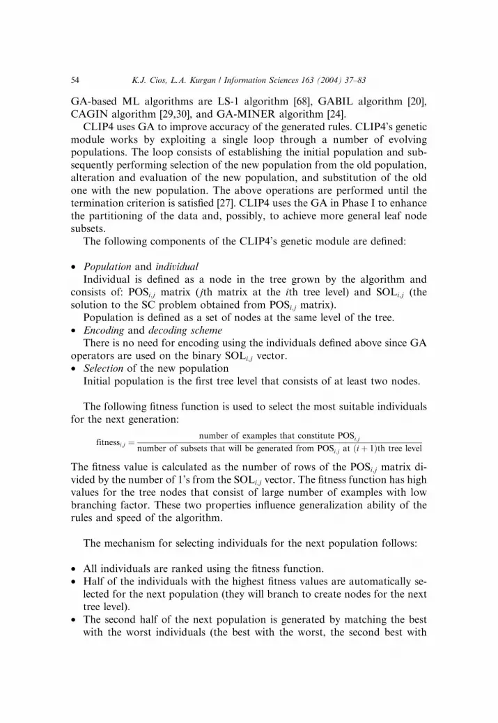
CLIP4 uses GA to improve accuracy of the generated rules. CLIP4’s genetic
module works by exploiting a single loop through a number of evolvingpopulations. The loop consists of establishing the initial population and sub-
sequently performing selection of the new population from the old population,
alteration and evaluation of the new population, and substitution of the old
one with the new population. The above operations are performed until the
termination criterion is satisfied [27]. CLIP4 uses the GA in Phase I to enhance
the partitioning of the data and, possibly, to achieve more general leaf node
subsets.
The following components of the CLIP4’s genetic module are defined:
• Population and individual
Individual is defined as a node in the tree grown by the algorithm and
consists of: POSi;j matrix (jth matrix at the ith tree level) and SOLi;j (the
solution to the SC problem obtained from POSi;j matrix).
Population is defined as a set of nodes at the same level of the tree.
• Encoding and decoding scheme
There is no need for encoding using the individuals defined above since GAoperators are used on the binary SOLi;j vector.
• Selection of the new population
Initial population is the first tree level that consists of at least two nodes.
The following fitness function is used to select the most suitable individuals
for the next generation:
fitnessi;j ¼number of examples that constitute POSi;j
number of subsets that will be generated from POSi;j at ðiþ 1Þth tree level
The fitness value is calculated as the number of rows of the POSi;j matrix di-
vided by the number of 1’s from the SOLi;j vector. The fitness function has highvalues for the tree nodes that consist of large number of examples with low
branching factor. These two properties influence generalization ability of the
rules and speed of the algorithm.
The mechanism for selecting individuals for the next population follows:
• All individuals are ranked using the fitness function.
• Half of the individuals with the highest fitness values are automatically se-lected for the next population (they will branch to create nodes for the next
tree level).
• The second half of the next population is generated by matching the best
with the worst individuals (the best with the worst, the second best with

Fig. 5. Selection mechanism performed by the GA module.
K.J. Cios, L.A. Kurgan / Information Sciences 163 (2004) 37–83 55
the second worst, etc.), and applying GA operators to obtain new individu-als (new nodes on the tree). This matching promotes generation of new tree
branches that contain large number of examples.
An example of the selection mechanism used in CLIP4 is shown in Fig. 5.
• Operators
The GA module uses crossover and mutation operators. Both are applied
only to the SOLi;j vectors. The resulting ChildSOLi;j vector, together with thePOSi;j matrix of the parent with the higher fitness value, constitutes the new
individual. The selection of the SOLi;j matrix assures that the resulting indi-
vidual is consistent with the CLIP4 way of partitioning data.
Crossover
The crossover operator is defined as: ChildSOLi ¼ maxðParent1SOLi;Parent2SOLiÞ where: Parent1SOLi and Parent2SOLi are the ith values of
SOLi;j vectors of the two parent nodes. Similar crossover operators based on
min or max functions are called flat crossover [63] and BLX-a cross-over
[22].
Mutation
Random mutation, with 10% chance, flips a value in the ChildSOL vector to
1, regardless of the existing value. The probability of mutation was established
experimentally during the benchmarking tests.
Each 1 in the ChildSOL generates new branch, except for 1’s taken from the
SOLi;j of the parent with higher fitness value. They are discarded because theywould generate branches redundant with branches generated by the parent.
The example of the crossover operation is shown in Fig. 6.
• Termination criterion
Termination criterion checks if the bottom level of the tree is reached. The
entire evolution process of the GA module is shown in Fig. 7.
The GA module is used when running CLIP4 on small data that cover only
a small portion of the state space, which results in generating rules thatpotentially can cover not yet described part of the state space. Later in the
paper we show usefulness of the GA module.

Fig. 7. The evolution process performed by the GA module.
Fig. 6. Example of the crossover performed by the GA module.
56 K.J. Cios, L.A. Kurgan / Information Sciences 163 (2004) 37–83
3.3. Pruning
The CLIP4 algorithm uses the pre-pruning technique to prune the tree
during the process of generating the tree. The pre-pruning stops the learning
process early although some positive examples may be not covered, and while
some negative examples are still covered ([17,25,73]).
CLIP4 prunes the tree grown in Phase I as follows:
• First, it selects a number (defined by the pruning threshold) of best nodes on
the ith tree level. The selection is performed based on the goodness criterion
that is identical to the fitness function described in Section 3.2. Only the se-
lected nodes are used to branch into new nodes that are passed to the
ðiþ 1Þth tree level.
• Second, all redundant nodes that resulted from the branching process are
removed. Two nodes are redundant if one contains positive examples, whichare equal or form a subset of positive examples of the other node. The
redundant node with the smaller number of examples is pruned first.

K.J. Cios, L.A. Kurgan / Information Sciences 163 (2004) 37–83 57
• Third, after the redundant nodes are removed, each new node is evaluated
using the noise threshold. If the node contains less number of examples than
specified by the threshold then it is pruned.
The pre-pruning method used in the CLIP4 algorithm avoids some disad-
vantages of the basic pre-pruning. It preserves the consistency of the CLIP4
learning process because it never allows for the negative examples to be covered
by the rules. It also does not interfere with the completeness condition of the
rule generation process. The CLIP4’s pre-pruning increases accuracy of the
generated rules and lowers the complexity of the algorithm. An example of
pruning is shown in Fig. 8.
3.4. The data model
The CLIP4 algorithm generates a data model that consists of:
• Rules, which describe classes defined in the data.
• Ranked set of attributes and selectors, which can be used for feature selec-
tion and data analysis.
CLIP4 ranks attributes by assigning them a goodness value that quantifiestheir relevance to a particular learning task. The attribute ranking can be used
as a weighted feature selection tool. This approach to feature selection is
similar to ReliefF [45] and Relief [40,41] algorithms. CLIP4 ranks selectors in
the same way as it ranks the attributes. The ranking provides additional insight
into the information hidden in the data.
Feature selection is a process of finding a subset of features from the original
set of features, optimal in the sense of the defined goal and criterion of a feature
Fig. 8. Example of pruning when generating ðiþ 1Þth tree level from the ith tree level: (a) without
the GA module and (b) with GA module active.

58 K.J. Cios, L.A. Kurgan / Information Sciences 163 (2004) 37–83
selection task. In case of classification, the goal is to achieve the highest
predictive accuracy. Similar approaches for feature selection without signifi-
cant decrease of predictive accuracy, are described in [19,44].
Goodness of each attribute and selector is computed using the set of clas-sification rules. All attributes with goodness value greater than zero are
strongly relevant to the classification task. Strong relevancy means that the
attribute cannot be removed from an attribute set without decrease of accu-
racy. The other attributes are irrelevant and thus can be removed from the
data.
The attribute and selector goodness values are computed as follows:
• Each generated rule has a goodness value that is equal to the percentage va-lue of the training positive examples it covers. Each rule consists of one or
more pairs of selectors, i.e. attribute and its value.
• Each selector has a goodness value equal to the goodness of the rule it comes
from. Goodness of the same selectors from different rules is summed up, and
then scaled to the ð0; 100Þ range. 100 is assigned to the highest summed value
and remaining summed values are scaled accordingly.
• For each attribute, the sum of scaled goodness for all its selectors is com-
puted and divided by the number of attribute values to obtain the goodnessof the attribute.
The following example shows attribute and selector ranking on the MONKS1
data [70]:
• Number of instances: 432
• Number of attributes: 8
• Attribute information: class¼{0,1}, a1¼f1;2;3g, a2¼f1;2;3g, a3¼f1;2g,a4 ¼ f1; 2; 3g, a5 ¼ f1; 2; 3; 4g, a6 ¼ f1; 2g
• No missing values
The MONKS1 has target concept for class 1 described in the following
form: ða1 ¼ a2Þ or ða5 ¼ 1ÞThe CLIP4 algorithm generated the following rules:
Rule 1. If a5 6¼ 2 and a5 6¼ 3 and a5 6¼ 4 thenclass¼ 1
(covers 46% (29/62)positive examples)
Rule 2. If a1 6¼ 1 and a1 6¼ 2 and a2 6¼ 2 and
a2 6¼ 1 then class¼ 1
(covers 27% (17/62)
positive examples)
Rule 3. If a1 6¼ 1 and a1 6¼ 3 and a2 6¼ 3 and
a2 6¼ 1 then class¼ 1
(covers 24% (15/62)
positive examples)
Rule 4. If a1 6¼ 2 a1 6¼ 3 and a2 6¼ 2 and a2 6¼ 3
then class¼ 1
(covers 14% (9/62)
positive examples)
K.J. Cios, L.A. Kurgan / Information Sciences 163 (2004) 37–83 59
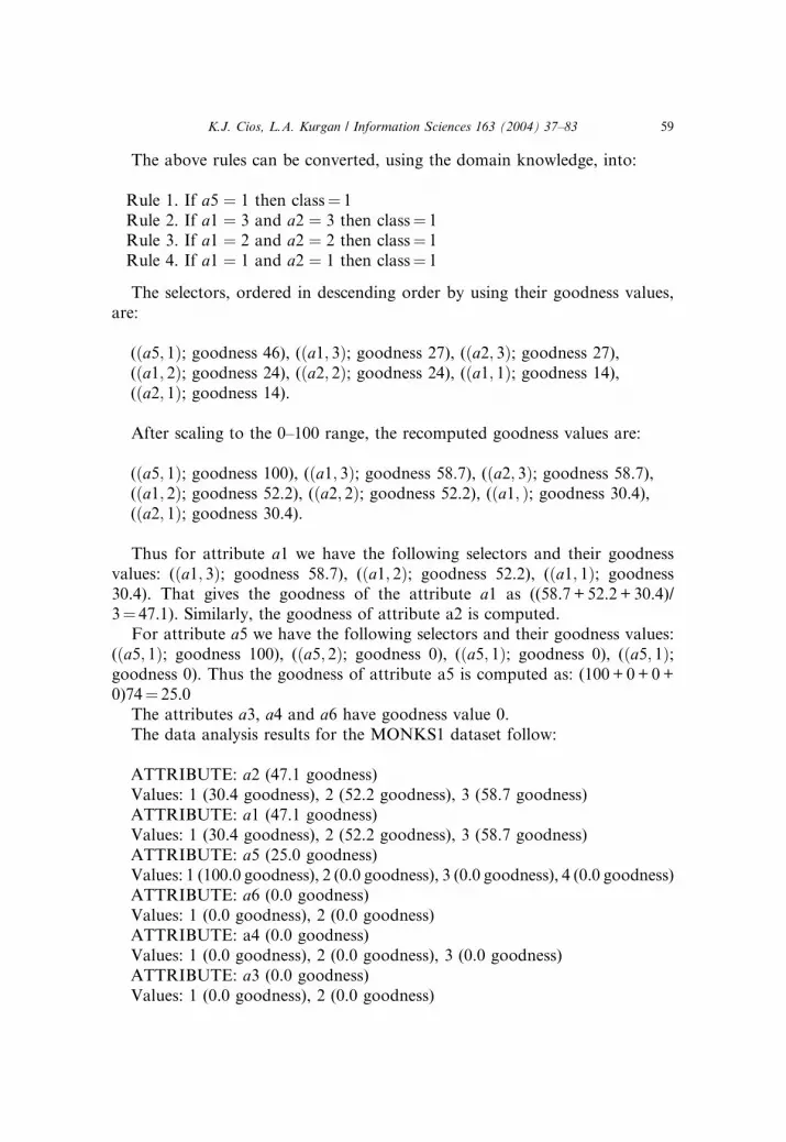
The above rules can be converted, using the domain knowledge, into:
The selectors, ordered in descending order by using their goodness values,
are:
(ða5; 1Þ; goodness 46), (ða1; 3Þ; goodness 27), (ða2; 3Þ; goodness 27),(ða1; 2Þ; goodness 24), (ða2; 2Þ; goodness 24), (ða1; 1Þ; goodness 14),(ða2; 1Þ; goodness 14).
After scaling to the 0–100 range, the recomputed goodness values are:
(ða5; 1Þ; goodness 100), (ða1; 3Þ; goodness 58.7), (ða2; 3Þ; goodness 58.7),(ða1; 2Þ; goodness 52.2), (ða2; 2Þ; goodness 52.2), (ða1; Þ; goodness 30.4),(ða2; 1Þ; goodness 30.4).
Thus for attribute a1 we have the following selectors and their goodness
values: (ða1; 3Þ; goodness 58.7), (ða1; 2Þ; goodness 52.2), (ða1; 1Þ; goodness
30.4). That gives the goodness of the attribute a1 as ((58.7 + 52.2 + 30.4)/3¼ 47.1). Similarly, the goodness of attribute a2 is computed.
For attribute a5 we have the following selectors and their goodness values:
(ða5; 1Þ; goodness 100), (ða5; 2Þ; goodness 0), (ða5; 1Þ; goodness 0), (ða5; 1Þ;goodness 0). Thus the goodness of attribute a5 is computed as: (100+ 0+ 0+
0)74¼ 25.0
The attributes a3, a4 and a6 have goodness value 0.
The data analysis results for the MONKS1 dataset follow:
ATTRIBUTE: a2 (47.1 goodness)
Values: 1 (30.4 goodness), 2 (52.2 goodness), 3 (58.7 goodness)
ATTRIBUTE: a1 (47.1 goodness)
Values: 1 (30.4 goodness), 2 (52.2 goodness), 3 (58.7 goodness)
ATTRIBUTE: a5 (25.0 goodness)
Values: 1 (100.0 goodness), 2 (0.0 goodness), 3 (0.0 goodness), 4 (0.0 goodness)
ATTRIBUTE: a6 (0.0 goodness)
Values: 1 (0.0 goodness), 2 (0.0 goodness)ATTRIBUTE: a4 (0.0 goodness)
Values: 1 (0.0 goodness), 2 (0.0 goodness), 3 (0.0 goodness)
ATTRIBUTE: a3 (0.0 goodness)
Values: 1 (0.0 goodness), 2 (0.0 goodness)
Rule 1. If a5 ¼ 1 then class¼ 1
Rule 2. If a1 ¼ 3 and a2 ¼ 3 then class¼ 1Rule 3. If a1 ¼ 2 and a2 ¼ 2 then class¼ 1
Rule 4. If a1 ¼ 1 and a2 ¼ 1 then class¼ 1

60 K.J. Cios, L.A. Kurgan / Information Sciences 163 (2004) 37–83
The attribute and selector ranking fully agrees with the target concept.
CLIP4 picked attributes a2 and a1 with the highest goodness value, and
attribute a5 with goodness above zero only for selector ða5; 1Þ. We see that the
attribute ranking allows removing attributes a3, a4 and a6 as irrelevant. Theselector ranking gives additional insight into the a5 attribute by showing that
only its value of 1 is strongly relevant to the target concept.
The feature and selector ranking can be used to:
• Select only relevant features, and discard irrelevant features from the data.
User can simply discard all attributes that have goodness of 0, and still have
correct model of the data. After irrelevant attributes are removed the algo-
rithm generates the same set of rules and thus describes the data with thesame accuracy.
Experimental results (Section 4.7) show that between 5% and 100% of the
features were retained (with several with less than 50%), while the original
accuracy of the rules was kept. The number of the retained attributes de-
pends on the strength of their association with the target class.
• Provide additional insight into properties of the data. The selector ranking
can help in analyzing the data in terms of relevance of the selectors to the
classification task.
4. Experimental results
The CLIP4 algorithm is extensively tested on several benchmark problems.
The results are presented in the following sections. The benchmarking consists
of tests that show the algorithm’s perfomance, and tests that aim to show
specific features of the algorithm.
The benchmarking results are presented in the form of accuracy of the rules,
their number, number of selectors used (complexity of the rules), and time ittakes to generate the rules.
4.1. Experiments configuration
Since an algorithm’s execution time varies between different hardware
configurations we used the SPEC benchmarking tests [69] for direct compari-
son of performance between various algorithms. SPEC benchmark tests con-
tain several programs that perform floating-point or integer computations,
which are intended to measure computer performance.
The general benchmarking results for CLIP4 are compared with the results
of [54], who compared 33 learning algorithms using publicly available datasets,and three different hardware configurations. By using the SPECint92 bench-

K.J. Cios, L.A. Kurgan / Information Sciences 163 (2004) 37–83 61
marking test they converted all execution times into the execution time
achieved when using the DEC3000 model 300 System (DEC). In this paper,
execution times of the CLIP4 algorithm are also converted into simulations on
the DEC System.There were two hardware configurations used to perform the tests: Intel
Pentium II 300 MHz with 128Mb RAM (I300), and Intel Pentium III 550 with
256Mb RAM (I550). The hardware configurations along with the corre-
sponding SPEC test results for all considered computer systems are given in
Table 2. To perform the recalculation of the execution times the following steps
are taken:
• The SPECint95 benchmarking test was used since our hardware configura-tion was not reported in the SPECint92 test. Thus, the Intel Pro Adler 150
MHz (I150) system was used as a bridge between the SPECint92 and SPE-
Cint95 benchmarking test, since it was reported on both of them.
• The CPU time ratio for I150 using DEC as the reference is calculated as fol-
lows: DEC time¼ (I150 time) * (SPECint92 for I150)/(SPECint92 for
DEC)� (I150 time) * 3.5.
• The ratio to transform the time from the I150 to I300 is calculated as:
I150 time¼ (I300 time) * (SPECint95 for I300)/(SPECint95 for I150)� (I300time) * 2.1.
• Both calculated above ratios are multiplied to calculate the CPU time be-
tween DEC and I300. The final formula for the I300 is:
DEC time� 7.3 * (I300 time).
Similar computations were performed for the I550 hardware configuration.
4.2. Datasets
CLIP4 was tested on 27 datasets. The range of the benchmarking is char-
acterized by:
Table 2
Computer hardware configuration used in the benchmarking tests and the corresponding results of
the SPEC benchmarking test
Workstation SPECint92
results
Workstation SPECint95
results
I150 Intel Pro 150
MHz (Alder)
243.9 1150 Intel Pro 150 MHz (Alder
System)
6.08
DEC DEC 3000
Model 300
66.2 1300 Intel Pentium II 300 MHz
SE440BX2
12.9
1550 Intel Pentium III 550 MHz 22.3

62 K.J. Cios, L.A. Kurgan / Information Sciences 163 (2004) 37–83
• The size of training datasets: between 150 and about 30 K examples.
• The size of testing datasets: between 45 and 565 K examples.
• The number of attributes: between 4 and 1558.
• The number of classes: between 2 and 10.
The datasets were obtained from the University of California at Irvine
(UCI) Machine Learning Repository [3], and from StatLog project datasets
repository [71]. Summary information about the datasets is given in Table 3.
The following datasets from the UCI were used:
1. Wisconsin breast cancer (bcw)
2. Contraceptive method choice (cmc)3. StatLog heart disease (hea) (originally from the StatLog project reposi-
tory)
4. Boston Housing (bos) (originally from the StatLog project repository)
5. LED display (led)
6. BUPA liver disorder (bld)
7. PIMA Indian diabetes (pid)
8. StatLog satellite image (sat) (originally from the StatLog project reposi-
tory)9. Image segmentation (seg) (originally from the StatLog project reposi-
tory)
10. Thyroid disease (thy)
11. StatLog vehicle silhouette (veh) (originally from the StatLog project repos-
itory)
12. Congressional voting records (vot)
13. Waveform (wav)
14. TA evaluation (tae)15. SPECT heart imaging (SPECT)
16. Adult (adult)
17. Internet advertisement (iad)
18. Mushrooms (mush)
19. Iris plant (iris)
20. Car evaluation (car)
21. Ionosphere (ion)
22. Forest CoverType (forc)23. Monks problem that consists of the three datasets: Monk1, Monk2, and
Monk3 (m1, m2, m3)
The following datasets from the StatLog were used:
1. StatLog DNA (dna)
2. Attitude towards smoking restrictions (smo)
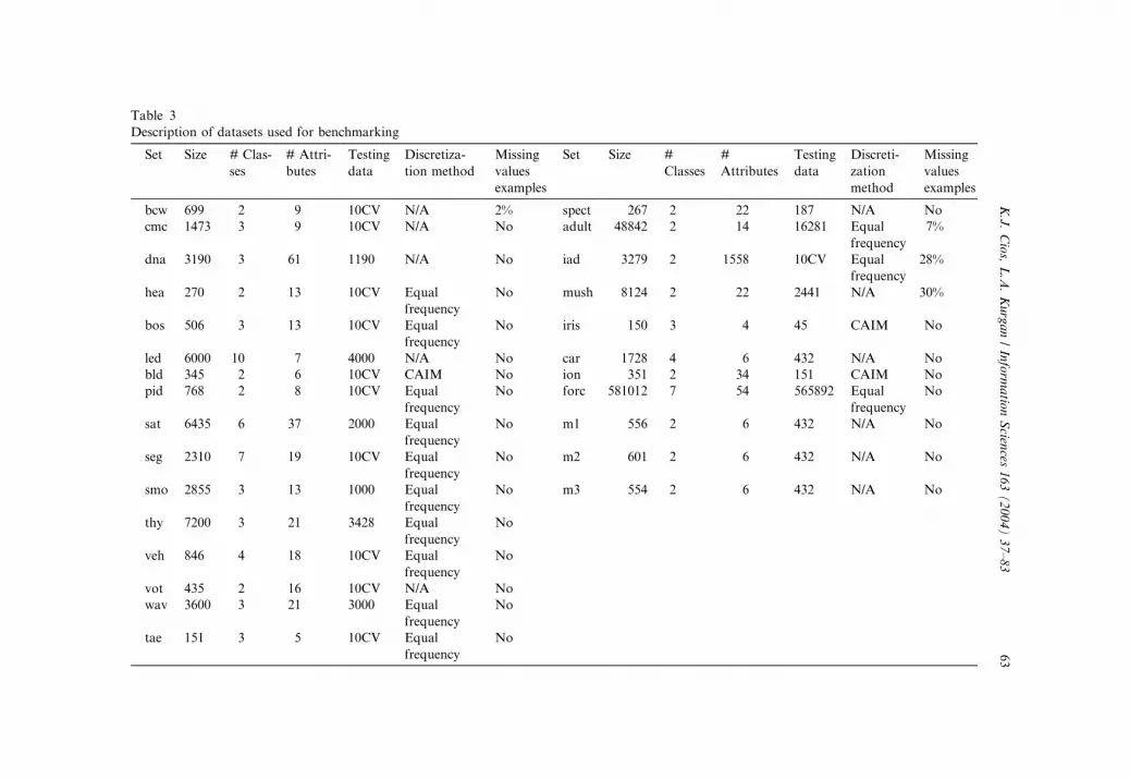
Table 3
Description of datasets used for benchmarking
Set Size # Clas-
ses
# Attri-
butes
Testing
data
Discretiza-
tion method
Missing
values
examples
Set Size #
Classes
#
Attributes
Testing
data
Discreti-
zation
method
Missing
values
examples
bcw 699 2 9 10CV N/A 2% spect 267 2 22 187 N/A No
cmc 1473 3 9 10CV N/A No adult 48842 2 14 16281 Equal
frequency
7%
dna 3190 3 61 1190 N/A No iad 3279 2 1558 10CV Equal
frequency
28%
hea 270 2 13 10CV Equal
frequency
No mush 8124 2 22 2441 N/A 30%
bos 506 3 13 10CV Equal
frequency
No iris 150 3 4 45 CAIM No
led 6000 10 7 4000 N/A No car 1728 4 6 432 N/A No
bld 345 2 6 10CV CAIM No ion 351 2 34 151 CAIM No
pid 768 2 8 10CV Equal
frequency
No forc 581012 7 54 565892 Equal
frequency
No
sat 6435 6 37 2000 Equal
frequency
No m1 556 2 6 432 N/A No
seg 2310 7 19 10CV Equal
frequency
No m2 601 2 6 432 N/A No
smo 2855 3 13 1000 Equal
frequency
No m3 554 2 6 432 N/A No
thy 7200 3 21 3428 Equal
frequency
No
veh 846 4 18 10CV Equal
frequency
No
vot 435 2 16 10CV N/A No
wav 3600 3 21 3000 Equal
frequency
No
tae 151 3 5 10CV Equal
frequency
No
K.J.Cios,L.A.Kurgan/Inform
atio
nScien
ces163(2004)37–83
63

64 K.J. Cios, L.A. Kurgan / Information Sciences 163 (2004) 37–83
4.3. Experiments and results
The general benchmarking tests were divided into two parts:
• The comparison test that compares the results with the results of [54]; when
the authors compared 33 ML algorithms using 16 datasets.
• The flexibility test uses additional 11 datasets. It was designed to test the
flexibility of CLIP4 using both artificial and real datasets, datasets that have
large number of attributes or examples, and datasets described by binary,
categorical, or continuous attributes.
For all test we employed the same testing procedures as in the tests per-formed by authors of the algorithms to which we compare CLIP4. Because of
that for some datasets we performed 10 fold cross-validation experiments, and
for others we used predefined test datasets; for details see Table 3.
4.3.1. The comparison test
The comparison test, Table 4, shows error rates, number of rules, number ofselectors, and the CPU execution time of CLIP4 for the 16 datasets. The CLIP4
results are compared to the results of Lim et al. (Lim, Loh and Shih, 2000).
Error rates (the maximum and minimum error rate values for all 33 tested
algorithms), median number of rules (the authors reported number of tree
leaves only for 21 decision tree algorithms), and CPU execution time (the
maximum and minimum CPU time values for all 33 tested algorithms) are
reported after them.
The mean error rate of the CLIP4 algorithm for the 16 datasets is 25.1%.The POLYCLASS algorithm [46], which achieved the smallest mean error rate,
has mean error rate of 19.5%. The Lim, Loh and Shih calculated statistical
significance of error rates, which showed that a difference between the mean
error rates of two algorithms is statistically significant at the 10% level if they
differ by more than 5.9%. They reported that 26 out of 33 algorithms were not
statistically significantly different from POLYCLASS. The CLIP4 falls within
the same category, which places it among the best ML algorithms.
CLIP4’s CPU execution time, which was calculated using the DEC hard-ware configuration, for the 16 datasets is 5.8 min. The Lim, Loh and Shih
reported that the mean CPU execution time for the 33 algorithms ranged be-
tween 6.9 s and 46.8 h. They categorized the tested algorithms into two groups:
algorithms that achieved mean CPU execution time below 10 min (22 algo-
rithms) and algorithms above the 10 min (11 algorithms). CLIP4 falls into the
first category. It is important to note that the POLYCLASS algorithm had
3.2 h mean execution time.
The CLIP4 algorithm achieves error rates that are statistically similar to thealgorithm that achieved the smallest error rates among all the algorithms tes-

Table 4
The comparison test results
Set Reported error
rates for the 33
ML algorithms
CLIP4
error rates
Reported median
# of leaves/rules
for the 21 algo-
rithms
CLIP4
# of
rules
Reported CPU time
for the 33 ML algo-
rithms
CLIP4 CPU time (s) CLIP4 # of
selectors
Min Max Min (s) Max (h) 1300 DEC¼ I300 * 7.3
bcw 3 9 5 7 4.2 4s 2.7 0.7 5.1 121.6
cmc 43 60 53 15 8 12s 23.9 6.3 46 60.7
dna 5 38 9 13 8 2s 475.2 90.8 662.8 90
hea 14 34 28 6 11.6 4s 3.3 0.3 2.2 192.3
bos 22 31 29 11 10.5 9s 5.5 4.9 35.8 133.5
led 27 82 29 24 41 1s 12.4 22.8 166.4 189
bld 28 43 37 10 9.7 5s 1.5 0.9 6.6 272.4
pid 22 31 29 7 4 7s 2.5 0.8 5.8 64.1
sat 10 40 20 63 61 8s 73.2 506.4 3696.7 3199
seg 2 52 14 39 39.2 28s 75.6 84.2 614.6 1169.9
smo 30 45 32 2 18 1s 3.8 12.4 90.5 242
thy 1 89 1 12 4 3s 16.1 23.5 164.2 119
veh 15 49 44 38 21.3 14s 14.1 6.2 45.3 380.7
vot 4 6 6 2 9.7 2s 25.2 0.6 4.4 51.7
wav 15 48 25 16 9 4s 4.3 5.9 43.1 85
tae 33 69 40 20 9.3 6s 10.2 0.1 0.7 273.2
Mean 17.1 45.4 25.1 17.8 16.8 6.9s 46.8 h 47.9 s 5.8 min 598.5
K.J.Cios,L.A.Kurgan/Inform
atio
nScien
ces163(2004)37–83
65

66 K.J. Cios, L.A. Kurgan / Information Sciences 163 (2004) 37–83
ted, and has CPU execution time smaller than 10 minutes. These results place it
among 18 top algorithms out of the 33 tested by Lim, Loh and Shih.
The mean number of rules generated by CLIP4 for the 16 datasets is 16.8.
Lim, Loh and Shih reported the median number of tree leaves (equivalent tothe number of rules) for the 21 tested decision tree algorithms, as 17.8. The
number of rules generated by the CLIP4 algorithm is lower than the reported
median. In addition, only 10 out of the 21 algorithms achieved lower mean
number of leaves than CLIP4.
The mean number of selectors generated by the CLIP4 algorithm for the 16
datasets was 589.5, which translates into about 35 selectors per rule.
4.3.2. The flexibility test
The flexibility test reports error rates, number of rules, number of selectors
and CPU execution time achieved by CLIP4 for the 11 datasets. For each
dataset, the error rate, the number of rules (or tree leaves), and the reference
where these results were reported, are shown in Table 5. The bold values in the
second and fourth columns describe the lowest reported error rates and the
minimum number of rules.For three datasets (adult, car, m2), two types of results, depending on the
user-chosen CLIP4’s thresholds (see Section 3.1.5), are shown. The first set of
results was generated with the aim of minimizing the error rates, and the
second by a user who aims to generate low number of rules at the price of
slightly higher error rates. The results for these datasets are shown, as high-
lighted rows, in Table 5, and can be summarized as follows:
• adult dataset: 3.1% error rate increase as a trade-off for generating 3.5 timesless rules;
• car dataset: 2.7% error rate increase as a trade-off for generating 1.5 times
less rules;
• m2 dataset: 7.5% error rate increase as a trade-off for generating 2.4 times
less rules.
Adjusting the thresholds allows the user to significantly decrease number of
the generated rules at the cost of slight increase of the error rate. In manyapplications, where it is important to understand the generated rules, the latter
may be desired.
The flexibility of the CLIP4 algorithm was tested by applying the algorithm
to the datasets with large number of examples (adult dataset) and large number
of attributes (iad dataset).
The error rate for the adult dataset is the same as the best reported rate for
the FSS Na€ıve Bayes algorithm. On the other hand, when error rate is traded
for decrease in the number of rules, 71 instead of 254 rules are generated, at theexpense of 3.1% higher error rate. Both sets of rules use on average about 105
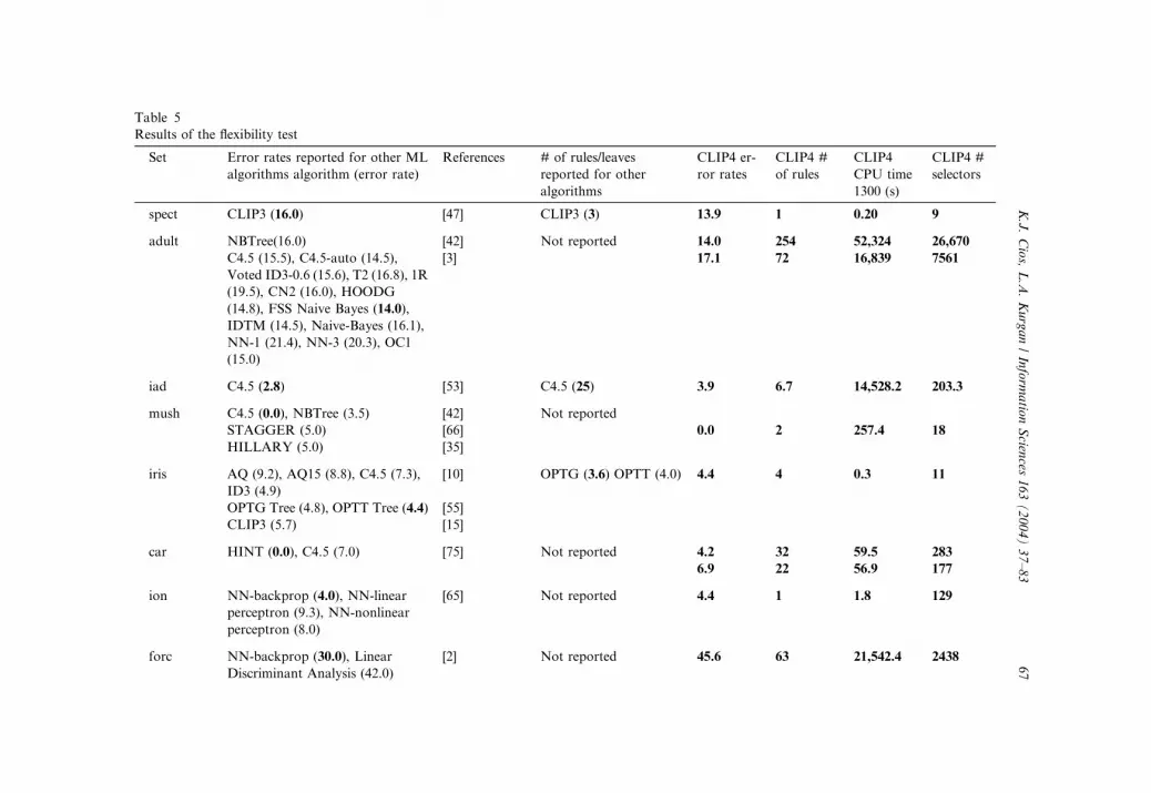
Table 5
Results of the flexibility test
Set Error rates reported for other ML
algorithms algorithm (error rate)
References # of rules/leaves
reported for other
algorithms
CLIP4 er-
ror rates
CLIP4 #
of rules
CLIP4
CPU time
1300 (s)
CLIP4 #
selectors
spect CLIP3 (16.0) [47] CLIP3 (3) 13.9 1 0.20 9
adult NBTree(16.0) [42] Not reported 14.0 254 52,324 26,670
C4.5 (15.5), C4.5-auto (14.5),
Voted ID3-0.6 (15.6), T2 (16.8), 1R
(19.5), CN2 (16.0), HOODG
(14.8), FSS Naive Bayes (14.0),
IDTM (14.5), Naive-Bayes (16.1),
NN-1 (21.4), NN-3 (20.3), OC1
(15.0)
[3] 17.1 72 16,839 7561
iad C4.5 (2.8) [53] C4.5 (25) 3.9 6.7 14,528.2 203.3
mush C4.5 (0.0), NBTree (3.5) [42] Not reported
STAGGER (5.0) [66] 0.0 2 257.4 18
HILLARY (5.0) [35]
iris AQ (9.2), AQ15 (8.8), C4.5 (7.3),
ID3 (4.9)
[10] OPTG (3.6) OPTT (4.0) 4.4 4 0.3 11
OPTG Tree (4.8), OPTT Tree (4.4) [55]
CLIP3 (5.7) [15]
car HINT (0.0), C4.5 (7.0) [75] Not reported 4.2 32 59.5 283
6.9 22 56.9 177
ion NN-backprop (4.0), NN-linear
perceptron (9.3), NN-nonlinear
perceptron (8.0)
[65] Not reported 4.4 1 1.8 129
forc NN-backprop (30.0), Linear
Discriminant Analysis (42.0)
[2] Not reported 45.6 63 21,542.4 2438
K.J.Cios,L.A.Kurgan/Inform
atio
nScien
ces163(2004)37–83
67
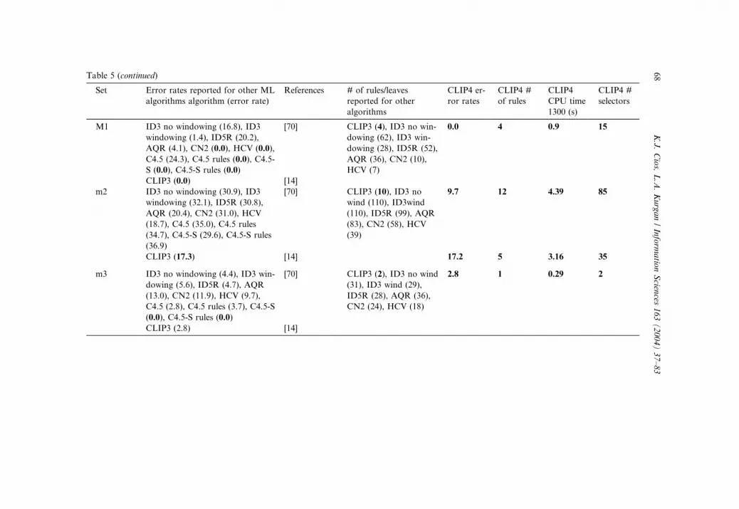
Table 5 (continued)
Set Error rates reported for other ML
algorithms algorithm (error rate)
References # of rules/leaves
reported for other
algorithms
CLIP4 er-
ror rates
CLIP4 #
of rules
CLIP4
CPU time
1300 (s)
CLIP4 #
selectors
M1 ID3 no windowing (16.8), ID3
windowing (1.4), ID5R (20.2),
AQR (4.1), CN2 (0.0), HCV (0.0),
C4.5 (24.3), C4.5 rules (0.0), C4.5-
S (0.0), C4.5-S rules (0.0)
[70] CLIP3 (4), ID3 no win-
dowing (62), ID3 win-
dowing (28), ID5R (52),
AQR (36), CN2 (10),
HCV (7)
0.0 4 0.9 15
CLIP3 (0.0) [14]
m2 ID3 no windowing (30.9), ID3
windowing (32.1), ID5R (30.8),
AQR (20.4), CN2 (31.0), HCV
(18.7), C4.5 (35.0), C4.5 rules
(34.7), C4.5-S (29.6), C4.5-S rules
(36.9)
[70] CLIP3 (10), ID3 no
wind (110), ID3wind
(110), ID5R (99), AQR
(83), CN2 (58), HCV
(39)
9.7 12 4.39 85
CLIP3 (17.3) [14] 17.2 5 3.16 35
m3 ID3 no windowing (4.4), ID3 win-
dowing (5.6), ID5R (4.7), AQR
(13.0), CN2 (11.9), HCV (9.7),
C4.5 (2.8), C4.5 rules (3.7), C4.5-S
(0.0), C4.5-S rules (0.0)
[70] CLIP3 (2), ID3 no wind
(31), ID3 wind (29),
ID5R (28), AQR (36),
CN2 (24), HCV (18)
2.8 1 0.29 2
CLIP3 (2.8) [14]
68
K.J.Cios,L.A.Kurgan/Inform
atio
nScien
ces163(2004)37–83

-16
-8
0
8
16
spect adult iad mush iris car ion forc m1 m2 m3
Comparison of the reported error rates with CLIP4 error rates (positive values mean improvement)
erro
r rate
s [%
]
Reported MIN Reported MEAN Reported MEDIAN
Fig. 9. Comparison of CLIP4 error rates with error rates reported in the literature, for the datasets
used in the flexibility test.
K.J. Cios, L.A. Kurgan / Information Sciences 163 (2004) 37–83 69
selectors per rule. Thus, the complexity of the rules does not change when the
number of rules is greatly reduced.
The error rate for the iad dataset is 3.9%, when the best reported error rate
for this dataset was 2.8% for C4.5 algorithm. However, CLIP4 generated only6.7 rules, which is 3.7 times less than the number of rules generated by C4.5.
The CLIP4 rules use only 30 selectors per rule, despite the fact that the iad
dataset has 1558 attributes and over 3100 possible selectors.
CLIP4 handles highly dimensional data by generating small sets of rules
with the same error rates as the best reported algorithms, while being flexi-
bile in deciding whether the low error rate or low number of rules is the
priority.
Fig. 9 compares error rates achieved by CLIP4 and error rates reported inthe literature. For the 11 dataset, the minimum, mean and median error rates
were calculated and the difference between each of these values and the CLIP4
error rate is plotted. For example, a positive value for the reported minimum
error rates for the SPECT dataset means that the CLIP4 achieved lower error
rate than any other reported error rate.
CLIP4 has the smallest error rate among the reported error rates for six out
of 11 datasets. For eight out of 11 datasets, the CLIP4 has lower error rate than
the mean or median reported error rate. The results for the m2 dataset showthat even when trading decrease in the error rate for smaller number of rules,
the error rate is lower than the lowest reported error rate and the number of
generated rules is twice smaller than the smallest reported number of rules.
The number of rules was reported only for six datasets. The CLIP4 algo-
rithm generated the smallest number of rules for five out of these six datasets,
and for the sixths dataset it generated just 0.4 rule more.
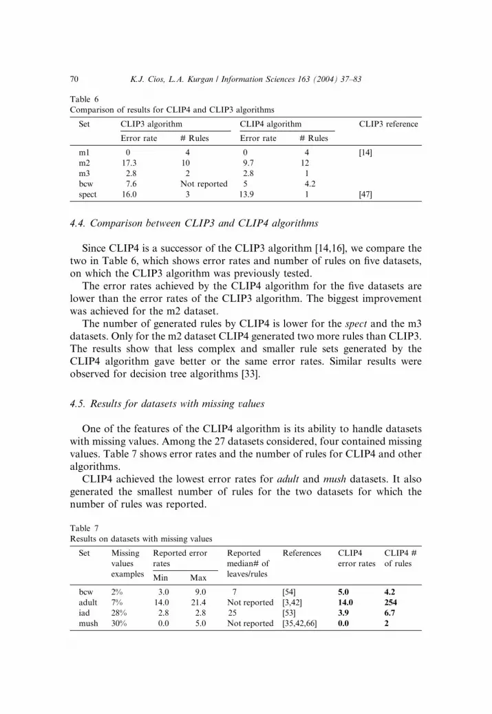
Table 6
Comparison of results for CLIP4 and CLIP3 algorithms
Set CLIP3 algorithm CLIP4 algorithm CLIP3 reference
Error rate # Rules Error rate # Rules
m1 0 4 0 4 [14]
m2 17.3 10 9.7 12
m3 2.8 2 2.8 1
bcw 7.6 Not reported 5 4.2
spect 16.0 3 13.9 1 [47]
70 K.J. Cios, L.A. Kurgan / Information Sciences 163 (2004) 37–83
4.4. Comparison between CLIP3 and CLIP4 algorithms
Since CLIP4 is a successor of the CLIP3 algorithm [14,16], we compare the
two in Table 6, which shows error rates and number of rules on five datasets,
on which the CLIP3 algorithm was previously tested.
The error rates achieved by the CLIP4 algorithm for the five datasets are
lower than the error rates of the CLIP3 algorithm. The biggest improvement
was achieved for the m2 dataset.
The number of generated rules by CLIP4 is lower for the spect and the m3
datasets. Only for the m2 dataset CLIP4 generated two more rules than CLIP3.The results show that less complex and smaller rule sets generated by the
CLIP4 algorithm gave better or the same error rates. Similar results were
observed for decision tree algorithms [33].
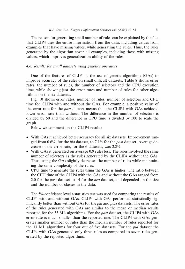
4.5. Results for datasets with missing values
One of the features of the CLIP4 algorithm is its ability to handle datasets
with missing values. Among the 27 datasets considered, four contained missing
values. Table 7 shows error rates and the number of rules for CLIP4 and other
algorithms.
CLIP4 achieved the lowest error rates for adult and mush datasets. It also
generated the smallest number of rules for the two datasets for which thenumber of rules was reported.
Table 7
Results on datasets with missing values
Set Missing
values
examples
Reported error
rates
Reported
median# of
leaves/rules
References CLIP4
error rates
CLIP4 #
of rules
Min Max
bcw 2% 3.0 9.0 7 [54] 5.0 4.2
adult 7% 14.0 21.4 Not reported [3,42] 14.0 254
iad 28% 2.8 2.8 25 [53] 3.9 6.7
mush 30% 0.0 5.0 Not reported [35,42,66] 0.0 2
K.J. Cios, L.A. Kurgan / Information Sciences 163 (2004) 37–83 71
The reason for generating small number of rules can be explained by the fact
that CLIP4 uses the entire information from the data, including values from
examples that have missing values, while generating the rules. Thus, the rules
generated by the algorithm cover all examples, including those with missingvalues, which improves generalization ability of the rules.
4.6. Results for small datasets using genetics operators
One of the features of CLIP4 is the use of genetic algorithms (GAs) to
improve accuracy of the rules on small difficult datasets. Table 8 shows errorrates, the number of rules, the number of selectors and the CPU execution
time, while showing just the error rates and number of rules for other algo-
rithms on the six datasets.
Fig. 10 shows error rates, number of rules, number of selectors and CPU
time for CLIP4 with and without the GAs. For example, a positive value of
the error rate for the post dataset means that the CLIP4 with GAs achieved
lower error rate than without. The difference in the number of selectors is
divided by 50 and the difference in CPU time is divided by 500 to scale thegraph.
Below we comment on the CLIP4 results:
• With GAs it achieved better accuracy for all six datasets. Improvement ran-
ged from 0.6%, for the bld dataset, to 7.1% for the post dataset. Average de-
crease of the error rate, for the 6 datasets, was 2.8%.
• With GAs it generated on average 0.9 rules less. The rules involved the same
number of selectors as the rules generated by the CLIP4 without the GAs.Thus, using the GAs slightly decreases the number of rules while maintain-
ing the same complexity of the rules.
• CPU time to generate the rules using the GAs is higher. The ratio between
the CPU time of the CLIP4 with the GAs and without the GAs ranged from
2.0 for the post dataset to 14 for the hea dataset, and depended on the size
and the number of classes in the data.
The 5% confidence level t-statistics test was used for comparing the results ofCLIP4 with and without GAs. CLIP4 with GAs performed statistically sig-
nificantly better than without GAs for the pid and post datasets. The error rates
of the rules generated with GAs are similar to the mean or median results
reported for the 33 ML algorithms. For the post dataset, the CLIP4 with GAs
error rate is much smaller than the reported one. The CLIP4 with GAs gen-
erates smaller number of rules than the median number of rules reported for
the 33 ML algorithms for four out of five datasets. For the pid dataset the
CLIP4 with GAs generated only three rules as compared to seven rules gen-erated by the reported algorithms.

Table 8
Results of CLIP4 with and without GAs
Set Size Reported error rates CLIP4 without GAs CLIP4 with GAs
Min Max # of rules/
leaves
Reference Error
rates
#
Rules
CPU time
1300 (s)
# of
selectors
Error
rates
#
Rules
CPU time
1300 (s)
# of
selectors
bld 345 28 43 10 [54] 36.6 9.7 0.9 272.4 36.0 9.6 5.7 273.9
pid 768 22 31 7 29.3 4 0.8 64.1 26.2 4 6.3 61.6
hea 270 14 34 6 27.8 11.6 0.3 192.3 26.3 10.7 4.2 169.8
sat 6435 10 40 63 20.5 61 506.4 3199 19.1 57 2402.1 3010
veh 846 15 49 38 43.5 21.3 6.2 380.7 40.4 21 49.8 360.1
post 90 48 48 Not reported [8] 46.4 18 1.0 88 39.3 18 2.0 92
72
K.J.Cios,L.A.Kurgan/Inform
atio
nScien
ces163(2004)37–83

-4
-2
0
2
4
6
bld pid hea sat veh postComparison between CLIP4 with and without genetic opeartors (positive values mean improvement)
error rates difference # rules difference # selectors difference / 50 CPU time difference / 500
Fig. 10. Comparison of the results with and without GAs.
K.J. Cios, L.A. Kurgan / Information Sciences 163 (2004) 37–83 73
Better accuracy and smaller number of rules generated with GAs show that
the use of GAs improves the results not by increasing the number of the
generated rules but by improving generalization ability of the rules so they
cover previously uncovered part(s) of the state space. GAs should be used only
for relatively small datasets because of high computational cost.
4.7. Results of feature selection via attribute ranking
The ranking of features can be used to select relevant features. CLIP4 ranks
features by assigning to them goodness values. If a feature has goodness value
equal to zero then it can be removed from the data, and CLIP4 will generate
the same set of rules as using all features. CLIP4 selects all features with
goodness values that are greater than zero as features that are strongly relevantto the classification task.
Table 9 shows the number of strongly relevant features, selected by CLIP4,
for 27 datasets.
CLIP4 discovered that all features are strongly relevant for nine out of 27
datasets. For eight datasets the CLIP4 algorithm discovered that only less than
50% of the original features are necessary to maintain minimum error rate.
These datasets are:
• iad: 5% (73.7/1558) of features were discovered as strongly relevant,
• ion: 15% (5/34) of features were discovered as strongly relevant,
• mush: 23% (5/22) of features were discovered as strongly relevant,
• spect: 32% (7/22) of features were discovered as strongly relevant,
• dna: 33% (20/61) of features were discovered as strongly relevant,
• m3: 33% (2/6) of features were discovered as strongly relevant,
• thy: 43% (9/21) of features were discovered as strongly relevant,
• m1: 50% (3/6) of features were discovered as strongly relevant.
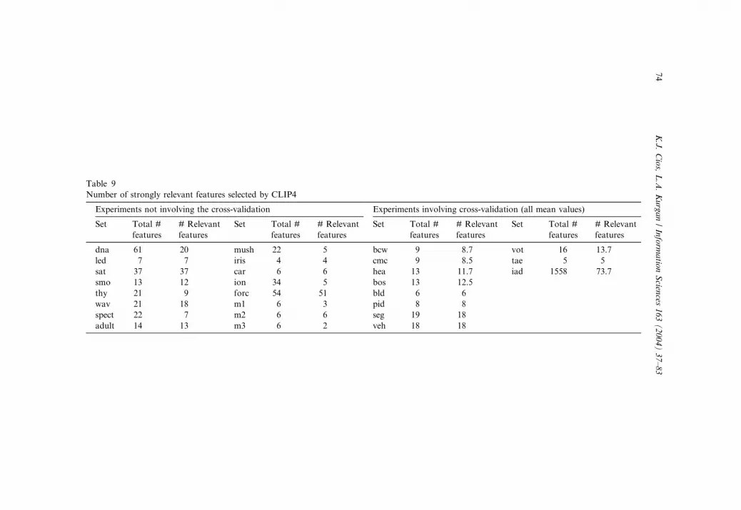
Table 9
Number of strongly relevant features selected by CLIP4
Experiments not involving the cross-validation Experiments involving cross-validation (all mean values)
Set Total #
features
# Relevant
features
Set Total #
features
# Relevant
features
Set Total #
features
# Relevant
features
Set Total #
features
# Relevant
features
dna 61 20 mush 22 5 bcw 9 8.7 vot 16 13.7
led 7 7 iris 4 4 cmc 9 8.5 tae 5 5
sat 37 37 car 6 6 hea 13 11.7 iad 1558 73.7
smo 13 12 ion 34 5 bos 13 12.5
thy 21 9 forc 54 51 bld 6 6
wav 21 18 m1 6 3 pid 8 8
spect 22 7 m2 6 6 seg 19 18
adult 14 13 m3 6 2 veh 18 18
74
K.J.Cios,L.A.Kurgan/Inform
atio
nScien
ces163(2004)37–83

Table 10
Comparison of feature selection results between CLIP4 and feature selection algorithms
Set Total #
features
CLIP4 #
relevant
features
Reported results
Plain ML
algorithm
Feature selection algorithm #
selected features (algorithm)
References
bcw 10 9.8 7(C4.5)
9.1(ID3)
3.9(C4.5-BSF), 5.9(NB-BSF),
5.3(ID3-BSF)
[43]
pid 8 8 8(C4.5),
8(1D3)
4.8(C4.5-BSF), 4.4(NB-BSF),
5.7(ID3-BSF)
[43]
5.3(FSV), 6(SVM) [6]
8(ReliefF 0), 4(ReliefF 0.01),
6(CFS)
[32]
mush 22 5 9.5(CFS) [31]
4.2(MDL) [62]
vot 16 13.7 16(ReliefF 0), 16(ReliefF 0.01) [32]
8.2(CFS) [31]
hea 13 11.7 13(ReliefF 0), 12(ReliefF 0.01),
7(CFS)
[32]
ion 34 5 33(ReliefF 0), 33(ReliefF 0.01),
16(CFS)
[32]
10.4 (FSV)6, 11.1 (SVM)6 [6]
seg 19 18 18(ReliefF 0), 15(ReliefF 0.01),
10(CFS)
[32]
bos 13 12.5 9(ReliefF), 4(CFS) [32]
bld 6 6 4.5(FSV), 5.8(SVM) [6]
m1 6 3 5(C4.5),
6(ID3)
3(C4.5-BSF), 4(NB-BSF),
3(ID3-BSF)
[43]
3(MDL) [62]
m2 6 6 6(C4.5),
6(ID3)
3(ID3-BSF) [43]
5.2(MDL) [62]
m3 6 2 2(C4.5),
6(ID3)
2(C4.5-BSF), 2(NB-BSF),
2(ID3-BSF)
[43]
3(B&B), 2(DTM), 4(Focus),
3(LVW)
[31]
2.3(MDL) [62]
K.J. Cios, L.A. Kurgan / Information Sciences 163 (2004) 37–83 75
For the first three datasets, the user can achieve over 75% compression rate
by removing all irrelevant attributes and still maintain the same error rate.
Table 10 shows the reported in the literature results that consist of the
number of features selected by a feature selection algorithm for the 12 datasets
and the number of features selected by a machine learning algorithm for the
five datasets. These results are compared with the results achieved by CLIP4.
For five datasets for which the number of selected features by a ML algo-
rithm is reported, CLIP4 selected similar to C4.5 number of strongly relevantfeatures, and smaller number of features than ID3. The difference between the
feature selection results of the CLIP4 and any other ML algorithms is that the
CLIP4 additionally ranks the selected features by assigning goodness values to
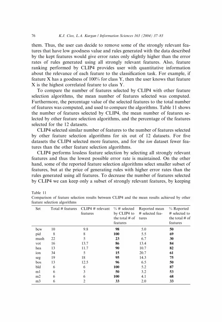
76 K.J. Cios, L.A. Kurgan / Information Sciences 163 (2004) 37–83
them. Thus, the user can decide to remove some of the strongly relevant fea-
tures that have low goodness value and rules generated with the data described
by the kept features would give error rates only slightly higher than the error
rates of rules generated using all strongly relevant features. Also, featureranking performed by CLIP4 provides user with quantitative information
about the relevance of each feature to the classification task. For example, if
feature X has a goodness of 100% for class Y, then the user knows that feature
X is the highest correlated feature to class Y.
To compare the number of features selected by CLIP4 with other feature
selection algorithms, the mean number of features selected was computed.
Furthermore, the percentage value of the selected features to the total number
of features was computed, and used to compare the algorithms. Table 11 showsthe number of features selected by CLIP4, the mean number of features se-
lected by other feature selection algorithms, and the percentage of the features
selected for the 12 datasets.
CLIP4 selected similar number of features to the number of features selected
by other feature selection algorithms for six out of 12 datasets. For five
datasets the CLIP4 selected more features, and for the ion dataset fewer fea-
tures than the other feature selection algorithms.
CLIP4 performs lossless feature selection by selecting all strongly relevantfeatures and thus the lowest possible error rate is maintained. On the other
hand, some of the reported feature selection algorithms select smaller subset of
features, but at the price of generating rules with higher error rates than the
rules generated using all features. To decrease the number of features selected
by CLIP4 we can keep only a subset of strongly relevant features, by keeping
Table 11
Comparison of feature selection results between CLIP4 and the mean results achieved by other
feature selection algorithms
Set Total # features CLIP4 # relevant
features
% # selected
by CLIP4 to
the total # of
features
Reported mean
# selected fea-
tures
% Reported
# selected to
the total # of
features
bcw 10 9.8 98 5.0 50
pid 8 8 100 5.5 69
mush 22 5 23 6.7 30
vot 16 13.7 86 13.4 84
hea 13 11.7 90 10.7 82
ion 34 5 15 20.7 61
seg 19 18 95 14.3 75
bos 13 12.5 96 6.5 50
bld 6 6 100 5.2 87
m1 6 3 50 3.2 53
m2 6 6 100 4.1 68
m3 6 2 33 2.0 33

K.J. Cios, L.A. Kurgan / Information Sciences 163 (2004) 37–83 77
features that for instance have goodness value grater than some threshold
value.
Although CLIP4 selects more features than other feature selection algo-
rithms the feature selection process is performed by the algorithm, in additionto its main task of generating the rules. It is also done at a fraction of the
computational cost of feature selection performed by some feature selection
algorithms. Moreover, CLIP4 ranks the selected features, an operation very
rarely performed by classical feature selection algorithms.
4.7.1. Feature ranking
CLIP4 ranks features by assigning goodness values to them. The feature
ranking helps to quantify the correlation between a feature and the classifi-
cation task.
Table 12 shows results of feature ranking for 15 datasets for which no cross-
validation experiments were performed; the strongly relevant features alongwith their goodness values are shown.
Table 12
Results of the feature ranking performed by the CLIP4 algorithm
Set The ranked strongly relevant features: feature (goodness value)
dna 34 (29.5), 36 (27.4), 6 (25.6), 35 (22.0), 5 (10.0), 16 (6.54), 18 (4.52), 17 (4.52), 23 (4.31),
56 (3.88), 37 (3.88), 22 (3.88), 20 (3.88), 13 (3.88), 48 (3.23), 43 (1.29), 19 (0.5), 8 (0.5), 7
(0.5), 39 (0.43)
led Digit2 (71.7), Digit5 (67.3), Digit1 (65.1), Digit4 (59.4), Digit7 (58.7), Digit3 (52.3),
Digit6 (51.9)
sat 1 (60.7), 2 (59.5), 10 (54.3), 26 (51.2), 9 (48.9), 19 (47.9), 22 (47.8), 25 (47.7), 34 (45.4),
18 (44.8), 21 (42.4), 3 (42.3), 13 (41.3), 11 (40.4), 33 (38.0), 7 (34.5), 6 (33.0), 29 (29.8),
15 (29.8), 27 (29.4), 17 (29.4), 23 (28.5), 4 (28.0), 16 (26.7), 5 (25.4), 20 (24.4), 31 (24.0),
14 (22.1), 24 (19.8), 12 (19.6), 30 (18.2), 8 (17.7), 35 (17.5), 28 (16.2), 32 (15.3), 36 (6.34)
smo Knowledge (64.3), Education (62.8), Weight (51.7), Age (44.5), Smoking3 (21.5),
Smoking2 (19.8), Smoking1 (13.8), WorkToronto (10.3), Smoking4 (8.8), Sex (6.44),
WorkHome (4.94), Residence (1.72)
thy 17 (75.8), 21 (53.9), 19 (43.7), 1 (30.6), 20 (24.7), 16 (17.0), 8 (16.9), 3 (16.9), 6 (16.2)
wav 1 (78.8), 4 (66.8), 5 (64.7), 16 (61.6), 12 (59.2), 10 (56.1), 15 (55.9), 13 (55.9), 14 (54.6), 7
(54.3), 6 (51.6), 9 (51.1), 17 (48.7), 18 (36.0), 11 (34.2), 19 (33.1), 8 (21.9), 3 (6.51)
spect 21 (50.0), 18 (50.0), 17 (50.0), 16 (50.0), 10 (50.0), 8 (50.0), 7 (50.0)
adult workclass (65.1), occupation (62.3), education (54.3), capital-gain (53.3), age (49.3),
marital-status (40.7), hours-per-week (40.6), relationship (33.1), capital-loss (32.1),
race (23.7), fnlwgt (18.0), native-country (12.9), sex (0.16)
mush Spore-print-color (73.2), Habitat (70.5), Stalk-color-below-ring (53.6), Odor (27.4),
Stalk-surface-above-ring (13.3)
iris PetalLength (67.6), SepalLength (64.1), PetalWidth (30.8), SepalWidth (3.81)
car persons (72.4), safety (57.3), maint (55.1), lug_boot (43.1), doors (42.9), buying (42.1)
ion 9 (52.6), 26 (52.5), 8 (51.0), 22 (50.8), 10 (50.8)
M1 2 (47.1 goodness), 1 (47.1), 5 (25.0)
M2 5 (76.8), 4 (72.9), 1 (72.9), 2 (72.4), 3 (65.0), 6 (60.8)
M3 5 (75.0), 2 (66.7)
78 K.J. Cios, L.A. Kurgan / Information Sciences 163 (2004) 37–83
Only for the led, sat, car, iris and m2 datasets all the attributes had goodness
values greater than zero for all features, and thus were selected as the strongly
relevant attributes.
For the dna dataset only five out of 20 strongly relevant features hadgoodness values greater than 10%, and similarly for the smo dataset only eight
out of 12 strongly relevant features had goodness values greater than 10%.
For the led dataset, CLIP4 discovered that all the features are equally rel-
evant to the classification task. Similarly, for the spect and ion datasets, the
selected strongly relevant features were discovered to be equally relevant to the
classification task.
For the smo dataset, the knowledge, education, weight and age features were
discovered as significantly more relevant to the classification task as the othereight strongly relevant features. Similarly, the 17th, 21st and 43rd feature from
the thy dataset were discovered as significantly more relevant to the classifi-
cation task than the other six strongly relevant features.
The feature ranking performed by the CLIP4 algorithm reveals additional
information in addition to selecting the strongly relevant features.
CLIP4 also ranks selectors by assigning goodness values to them. The
selectors ranking provides still another insight into properties of the features. It
shows the importance of the specific feature values rather than importance ofthe entire attribute.
4.8. Analysis of the results
The purpose of benchmarking was to provide the answer to whether CLIP4
satisfies the four (see Section 1) goals of a good supervised inductive learningsystem.
1. Does CLIP4 generate rules that result in accurate classification?
The benchmarking tests show that it generates rules that accurately classify
new examples, even in the presence of noise. CLIP4 achieves error rates that
are statistically similar to error rates achieved by the most accurate algo-
rithm among the 33 algorithms tested.
2. Does CLIP4 generate simple rules?CLIP4 keeps the rules compact by pruning that prevents generation of rules
that cover small number of examples, and the new algorithm for solving the
SC problem that promotes generation of general rules. The benchmarking
tests show that CLIP4 generated small number of compact rules.
3. Does CLIP4 generate rules efficiently?
Efficiency of the algorithm was measured by the CPU execution time. The
CLIP4 uses pruning that greatly reduces its computational complexity. The
benchmarking tests showed that the average CPU execution time of CLIP4on the 16 datasets was 5.8 min. This result places CLIP4 among the 22
K.J. Cios, L.A. Kurgan / Information Sciences 163 (2004) 37–83 79
fastest algorithms out of the 33 state-of-the-art ML algorithms that achieved
the average CPU execution time below 10 min. The theoretical estimation of
the expected running time of the algorithm also shows that is can be suc-
cessfully applied to large datasets.4. Is CLIP4 flexible?
CLIP4 was tested on datasets consisting of thousands of examples and
hundreds of attributes (discrete numerical, discrete nominal, continuous,
binary), including noisy and missing value examples. The tests show that
CLIP4 achieves low error rates and generates small number of compact
rules.
The benchmarking tests also show that other features of the CLIP4 algo-rithm are very useful:
• Use of genetic algorithms to improve generalization abilities and error rates
of the generated rules on small data.
• Use of feature selection and ranking that is used as a feature selection and
data analysis tool.
• Mechanism for handling datasets with missing values, which uses the entire
information to improve error rates of the generated rules.
5. Summary and conclusions
One of the very important issues is the size and dimensionality of data that
can be processed by any given machine learning algorithm. Both, the re-
searchers and users need to deal with the problem that a system works for
‘‘three examples’’ but is not scalable [67]. Only few learning algorithms can dealwith large highly-dimensional data; CLIP4 algorithm is one of them.
Another issue is the flexibility of a learning algorithm. It should work with a
variety of datasets to be applicable to real-life problems. In summary, the main
advantages of the CLIP4 algorithm are:
• The unique feature of the algorithm is generation of rules from selectors that
involve inequalities. For domains where attributes have large number of dis-
crete values, and when majority of them are correlated with a single class,this feature results in generation of more compact or smaller number of
rules, as compared with rules that are based on equality selectors only.
• Its flexibility; it works with highly dimensional data due to its mechanisms of
pruning and solving the set covering problem.
• Its ability for providing solutions to multiple learning tasks; it does not only
generate classification rules but also performs feature selection and feature
and selector ranking, which helps in constructing accurate data models.
80 K.J. Cios, L.A. Kurgan / Information Sciences 163 (2004) 37–83
The CLIP4 algorithm incorporated ideas from domains like decision trees,
rule algorithms, genetic algorithms, feature selection algorithms, and discreti-
zation methods, to achieve its flexibility and functionality.
The key features of any state-of-the-art algorithm are its flexibility, appli-cability to a wide range of problems, and ability to solve multiple learning
tasks. The benchmarking tests show that the CLIP4 algorithm is applicable to
diverse types of data. They place it among the most efficient learning algo-
rithms. CLIP4 can perform simultaneously several learning tasks like rule
induction, feature selection, and feature and selectors ranking. Other features
of the CLIP4 algorithm are its ability to work with small, difficult datasets, and
its easy implementation since it uses only tables and lists.
Acknowledgements
The authors thank Dr Ivan Bratko for his comments that resulted in con-
siderable improvement of the article.
References
[1] M. Bellmore, H.D. Ratliff, Set covering and involuntary bases, Management Science 18
(1971) 3.
[2] J.A. Blackard, Comparison of Neural Networks and Discriminant Analysis in Predicting
Forest Cover Types, Ph.D. dissertation, Department of Forest Sciences, Colorado State
University, Fort Collins, Colorado, 1998.
[3] C.L. Blake, C.J. Merz, UCI Repository of Machine Learning Databases. Available from
<http://www.ics.uci.edu/~mlearn/MLRepository.html>. Irvine, CA: University of California,
Department of Information and Computer Science, 1998.
[4] M. Bohanec, I. Bratko, Trading accuracy for simplicity in decision trees, Machine Learning
Journal 15 (3) (1994) 223–250.
[5] E. Boros, P.L. Hammer, T. Ibaraki, A. Kogan, E. Mayoraz, I. Muchnik, An implementation
of logical analysis of data, IEEE Transactions on Knowledge and Data Engineering 12 (2)
(2000) 292–306.
[6] P.S. Bradley, O.L. Mangasarian, Feature selection via concave minimization and support
vector machines, in: Proceedings of the Fifteenth International Conference on Machine
Learning, San Francisco, CA, Morgan Kaufmann, 1998, pp. 82–90.
[7] I. Bratko, Machine learning in artificial intelligence, Artificial intelligence in Engineering 8 (3)
(1993) 159–164.
[8] A. Budihardjo, J. Grzymala-Busse, L. Woolery, Program LERS_LB 2.5 as a Tool for
Knowledge Acquisition in Nursing, in: Proceedings of the Fourth International Conference on
Industrial and Engineering Applications of AI and Expert Systems, 1991, pp. 735–740.
[9] J. Catlett, On changing continuous attributes into ordered discrete attributes, in: Proceedings
of European Working Session on Learning, 1991, pp. 164–178.
[10] J.Y. Ching, A.K.C. Wong, K.C.C. Chan, Class-dependent discretization for inductive learning
from continuous and mixed mode data, IEEE Transactions on Pattern Analysis and Machine
Intelligence 17 (7) (1995) 641–651.

K.J. Cios, L.A. Kurgan / Information Sciences 163 (2004) 37–83 81
[11] D. Chiu, A. Wong, B. Cheung, Information discovery through hierarchical maximum entropy
discretization and synthesis, in: G. Piatesky-Shapiro, W.J. Frowley (Eds.), Knowledge
Discovery in Databases, MIT Press, 1991.
[12] K.J. Cios, N. Liu, An Algorithm which Learns Multiple Covers via Integer Linear
Programming. Part I––The CLILP2 Algorithm, Kybernetes, 24:2, pp. 29–50 (The Norbert
Wiener Outstanding Paper Award), 1995.
[13] K.J. Cios, N. Liu, An Algorithm which Learns Multiple Covers via Integer Linear
Programming. Part II––experimental results and conclusions, Kybernetes 24 (3) (1995) 24–36.
[14] K.J. Cios, D.K. Wedding, N. Liu, CLIP3: Cover learning using integer programming,
Kybernetes 26 (4–5) (1997) 513–536.
[15] K.J. Cios, W. Pedrycz, R. Swiniarski, Data Mining Methods for Knowledge Discovery,
Kluwer, http://www.wkap.nl/book.htm/0-7923-8252-8, 1998.
[16] K.J. Cios, L. Kurgan, Hybrid inductive machine learning: An overview of CLIP algorithms, in:
L.C. Jain, J. Kacprzyk (Eds.), New Learning Paradigms in Soft Computing, Physica-Verlag
(Springer), 2001, pp. 276–322.
[17] P. Clark, T. Niblett, The CN2 algorithm, Machine Learning 3 (1989) 261–283.
[18] P. Clark, R. Boswell, Rule induction with CN2: Some recent improvements, in: Y. Kodratoff
(Ed.), Lecture Notes in Artificial Intelligence, Proceedings of European Working Session on
Learning, Springer-Verlag, 1991, pp. 151–163.
[19] M. Dash, H. Liu, Feature selection for classification, Intelligent Data Analysis 1 (1997) 131–
156.
[20] K.A. DeJong, W.M. Spears, D.F. Gordon, Using genetic algorithm for concept learning,
Machine Learning 13 (1993) 161–188.
[21] J. Dougherty, R. Kohavi, M. Sahami, Supervised and unsupervised discretization of
continuous features, in: Proceedings of the Twelfth International Conference on Machine
Learning, 1995, pp. 194–202.
[22] L.J. Eshelman, J.D. Shaffer, Real-coded genetic algorithms and interval schemata, in: D.L.
Whitley (Ed.), Foundations of Genetic Algorithms II, Morgan Kaufman, 1993, pp. 187–202.
[23] U.M. Fayyad, K.B. Irani, On the handling of continuous-valued attributes in decision tree
generation, Machine Learning 8 (1992) 87–102.
[24] I.W. Flockhart, N.J. Radcliffe, A genetic algorithm-based approach to data mining, Second
International Conference on Knowledge Discovery and Data Mining (KDD-96), 1996, pp.
299–302.
[25] J. F€urnkranz, FOSSIL: A robust relational learner, in: Proceedings of the Seventh European
Conference on Machine Learning (ECML-94), Catania, Italy, Springer-Verlag, 1994, pp. 122–
137.
[26] M.R. Garey, D.S. Johnson, Computers and Intractability: A Guide to the Theory of NP-
Completeness, Freeman, W.H. & Company, New York, 1979.
[27] D.E. Goldberg, Genetics Algorithm in Search, Optimization and Machine Learning, Addison-
Wesley, 1989.
[28] R.S. Grafinkel, G.L. Nembauser, Integer Programming, John Wiley & Sons, New York, 1972.
[29] D.P. Greene, S.F. Smith, Using coverage as a model building constraint in learning classifier
systems, Evolutionary Computation 2 (1) (1994) 67–91.
[30] D.P. Greene, S.F. Smith, Competition-based induction of decision models from examples,
Machine Learning 13 (1993) 229–257.
[31] M.A. Hall, L.A. Smith, Practical feature subset selection for machine learning, in:
Proceedings of the Twenty first Australian Computer Science Conference, Springer, 1998,
pp. 181–191.
[32] M.A. Hall, Correlation-based feature selection for discrete and numeric class machine
learning, in: Proceedings of the Seventeenth International Conference on Machine Learning,
Stanford University, CA, Morgan Kaufmann, 2000.

82 K.J. Cios, L.A. Kurgan / Information Sciences 163 (2004) 37–83
[33] R.C. Holte, Very simple classification rules perform well on most commonly used data sets,
Machine Learning 11 (1993) 63–90.
[35] W. Iba, J. Wogulis, P. Langley, Trading off simplicity and coverage in incremental concept
learning, in: Proceedings of the Fifth International Conference on Machine Learning, Ann
Arbor, Michigan, Morgan Kaufmann, 1988, pp. 73–79.
[36] J. Kacprzyk, G. Szkatula, An algorithm for learning from erroneous and incorrigible
examples, International Journal of Intelligent Systems 11 (1996) 565–582.
[37] R.M. Karp, Reducibility Among Combinatorial Problems, Complexity of Computer Com-
putations, Plenum Press, New York, 1972.
[38] K.A. Kaufman, R.S. Michalski, Learning from Inconsistent and Noisy Data: The AQ18
Approach, in: Proceedings of the Eleventh International Symposium on Methodologies for
Intelligent Systems, Warsaw, Poland, 1999.
[39] R. Kerber, ChiMerge: discretization of numeric attributes, in: Proceedings of Ninth
International Conference on Artificial Intelligence (AAAI-91), 1992, pp. 123–128.
[40] K. Kira, L.A. Rendell, The feature selection problem: traditional methods and a new
algorithm, in: Proceedings of the Tenth National Conference on Artificial Intelligence, MIT
Press, 1992, pp. 129–134.
[41] K. Kira, L.A. Rendell, A practical approach to feature selection, in: Proceedings of the Ninth
International Conference on Machine Learning, Morgan-Kaufmann, 1992.
[42] R. Kohavi, Scaling up the accuracy of Naive-Bayes classifiers: a decision-tree hybrid, in:
Proceedings of the Second International Conference on Knowledge Discovery and Data
Mining, 1996, pp. 202–207.
[43] R. Kohavi, G.H. John, Wrappers for feature subset selection, Artificial Intelligence 1–2 (1997)
273–324.
[44] D. Koller, M. Sahami, Toward optimal feature selection, in: Proceedings of the Thirteenth
International Conference on Machine Learning, Bari, Italy, 1996, pp. 284–292.
[45] I. Kononenko, Estimating attributes: analysis and extensions of relief, in: Proceedings of the
1994 European Conference on Machine Learning, Catania, Italy, 1994.
[46] C. Kooperberg, S. Bose, C.J. Stone, Polychotomous regression, Journal of the American
Statistical Association 92 (1997) 117–127.
[47] L.A. Kurgan, K.J. Cios, R. Tadeusiewicz, M. Ogiela, L.S. Goodenday, Knowledge discovery
approach to automated cardiac SPECT diagnosis, Artificial Intelligence in Medicine 23 (2)
(2001) 149–169.
[48] L.A. Kurgan, K.J. Cios, Discretization algorithm that uses class-attribute interdependence
maximization, in: Proceedings of the 2001 International Conference on Artificial Intelligence
(IC-AI-2001), Las Vegas, Nevada, 2001, pp. 980–987.
[49] L.A. Kurgan, K.J. Cios, DataSqueezer Algorithm that Generates Small Number of
Short Rules, IEE Proceedings: Vision, Image and Signal Processing, submitted, 2002.
[50] L.A. Kurgan, Meta Mining System for Supervised Learning, Ph.D. dissertation, University of
Colorado at Boulder, Department of Computer Science, 2003.
[51] L.A. Kurgan, K.J. Cios, Meta-Mining Architecture for Learning from Supervised Data,
submitted, 2003.
[52] L.A. Kurgan, K.J. Cios, CAIM Discretization Algorithm, IEEE Transactions of Knowledge
and Data Engineering 16 (2) (2004) 145–153.
[53] N. Kushmerick, Learning to remove internet advertisements, in: Proceedings of the Third
International Conference on Autonomous Agents, Seattle, 1999, pp. 175–181.
[54] T.-S. Lim, W-Y. Loh, Y-S. Shih, A comparison of prediction accuracy, complexity, and
training time of thirty-three old and new classification algorithms, Machine Learning 40 (2000)
203–228.
[55] D. Malerba, F. Esposito, G. Semeraro, A further comparison of simplification methods for
decision-tree induction, in: D. Fisher, H. Lenz (Eds.), Learning from Data: Artificial Intelli-
gence and Statistics V, Lecture Notes in Statistics, Springer Verlag, Berlin, 1996.

K.J. Cios, L.A. Kurgan / Information Sciences 163 (2004) 37–83 83
[56] R.S. Michalski, On the quasi-optimal solution of the general covering problem, in: Proceedings
of the Fifth International Symposium on Information Processing, A3:25–128, Bled, Yugosla-
via, 1969.
[57] R.S. Michalski, Discovering classification rules using variable-valued logic system VL1, in:
Proceedings of the Third International Joint Conference on Artificial Intelligence, 1973, pp.
162–172.
[58] R.S. Michalski, A theory and methodology of inductive learning, in: R. Michalski, J.
Carbonell, T.M. Mitchell (Eds.), Machine Learning, Tioga Press, 1983.
[59] R.S. Michalski, L. Mozetic, J. Hong, N. Lavrac, The multipurpose incremental learning
system AQ15 and its testing application to three medical domains, in: Proceedings of Fifth
National Conference on Artificial Intelligence, Morgan-Kaufmann, Philadelphia, PA, 1986,
pp. 1041–1045.
[61] B. Pfahringer, Compression-based discretization of continuous attributes, in: Proceedings of
the Twelfth International Conference on Machine Learning, 1995, pp. 456–463.
[62] B. Pfahringer, Compression-based feature subset selection, in: Proceedings of the IJCAI-95
Workshop on Data Engineering for Inductive Learning, Montreal, Canada, 1995, pp. 109–119.
[63] N.J. Radcliffe, Forma analysis and random respectful recombination, in: Proceedings of the
Fourth International Conference on Genetic Algorithms, Morgan-Kaufmann, 1991, pp. 222–
229.
[64] A. Ravindran, D.T. Phillips, J.J. Solberg, Operations Research, Principles and Practice, second
ed., John Wiley & Sons, 1987, pp. 1–69.
[65] V.G. Sigillito, S.P. Wing, L.V. Hutton, K.B. Baker, Classification of radar returns from the
ionosphere using neural networks, Johns Hopkins APL Technical Digest 10 (1989) 262–266.
[66] J.S. Schlimmer, Concept Acquisition through Representational Adjustment, (Technical Report
87-19), Ph.D. dissertation, Department of Information and Computer Science, University of
California, Irvine, 1987.
[67] R.C. Shank, Where is AI, AI Magazine, winter 1991, pp. 38–49.
[68] S.F. Smith, Adaptive learning systems, in: R. Forsyth (Ed.), Expert Systems: Principles and
Case Studies, Associated Book Publishers Ltd, 1984.
[69] SPEC, Standard Performance Evaluation Corporation. Available from <http://www.spec.org/
spec/>, 2001.
[70] S.B. Thrun, J. Bala, E. Bloedorn, I. Bratko, B. Cestnik, J. Cheng, K.D. Jong, S. Dzeroski,
R. Hamann, K. Kaufman, S. Keller, I. Kononenko, J. Kreuziger, R.S. Michalski, T. Mitchall,
P. Pachowicz, B. Roger, H. Vafaie, W.V. deVelde, W. Wenzel, J. Wnek, J. Zhang, The
MONK’s Problems: A Performance Comparison of Different Learning Algorithms, tech.
report CMU-CS-91-197, Computer Science Department, Carnegie Mellon University, 1991.
[71] P. Vlachos, StatLib Project Repository. Available from <http://lib.stat.cmu.edu>, 2000.
[72] J.R. Quinlan, Simplifying decision trees, International Journal of Man-Machine Studies 27
(1987) 221–334.
[73] J.R. Quinlan, Learning logical definitions from relations, Machine Learning 5 (1990) 239–
266.
[74] J.R. Quinlan, C4.5 Programs for Machine learning, Morgan-Kaufmann, 1993.
[75] B. Zupan, M. Bohanec, I. Bratko, J. Demsar, Machine learning by function decomposition, in:
Proceedings of the Fourteen International Conference on Machine Learning, Nashville, TN,
1997, pp. 421–429.