1

Abstract—A new method is presented to identify and to

characterize voltage dips measurements from power quality

survey. This method is based on the space vector transformation,

which describes the three power system voltages by one complex

variable – the space vector. Its representation in the complex

plane is used to classify voltage dips. Indeed, for a not disturbed

system voltages, the space vector represents a circle in the

complex plane with a radius equal to the nominal voltage. It

follows the same shape for balanced dips, but with a smaller

radius. For unbalanced dips, this shape becomes an ellipse with

parameters depending on the phase(s) in drop, dip severity and

phase angle shift. Further, space vector characteristics and zero

sequence voltage are used for a more precise determination of the

voltage dip type. The developed algorithm for voltage dips

classification is validated by EMTP simulations and measurement

data.

Index Terms—voltage dips (sags), characterization,

classification, monitoring, power quality, power system, space

vector.

I. INTRODUCTION

OLTAGE dips are one of the most serious power quality

problem and represent a major concern for the industry.

They may cause interruption of industrial processes and may

lead to economical losses and distorted quality products.

During the last years, equipments used in industrial plants have

become more sensitive to voltage dips as a result of

technology improvement and increased use of power

electronics devices [1,2]. Thus, the automatic analysis

classification and characterization of voltage dips have

become an essential requirement for power quality monitoring.

Three phase voltage dips are mainly characterized by their

duration, magnitudes and phase angle jumps. The last two

parameters determine the dip type (signature), which is

relevant for the dip severity, as well as for the dip origin and

location.

In order to determine the dip type, several methods are

proposed in the literature. The most intuitive approach directly

uses measured voltage waveforms for voltage dips

V. Ignatova is with the Laboratory of Electrical Engineering, Grenoble,

France (e-mail: vanya.ignatova@leg.ensieg.inpg.fr).

P. Granjon is with the Laboratory of Images and Signals, Grenoble,

France (e-mail: pierre.granjon@lis.inpg.fr).

S. Bacha is with the Laboratory of Electrical Engineering, Grenoble,

France (e-mail: seddik.bacha@leg.ensieg.inpg.fr).

F. Dumas is with Schneider Electric, Grenoble, France, (e-mail:

frederic.dumas@schneider-electric.com)

classification [3]. This method is easy to understand, but is not

able to extract the characteristics of measured dips and

consequently is not appropriate to automatic voltage dips

analysis.

Another method [4] compares the six RMS values of phase

and phase-to-phase voltages after removing the zero sequence

component. The dip type is determined from the lowest

magnitude voltage. This method does not give any phase

information and can not provide a full dip characterization.

A recent method proposed in [5,6] is based on the theory of

symmetrical components. It quantifies three phase unbalanced

voltage dips using one complex variable called characteristic

voltage. However, for a complete and precise dip

classification, additional characteristics are used, like zero

sequence voltage and PN factor.

In this paper a new method for dip classification and

characterization is developed. It is based on space vector

transformation and leads to a more concise representation of

voltage dips. The space vector methodology allows to extract

characteristic features of the dip, to determine its type and

evaluate its severity.

One of the main advantages of this method is the use of only

the space vector and zero sequence voltage for voltage dips

analysis. In addition, it offers an exhaustive classification and

complete characterization of three phase voltage dips.

This paper is organized as follows: Section II describes the

space vector transformation and its representation in the

complex plane. Section III deals with voltage dips

identification from space vector and zero sequence voltage.

Finally, the complete method for voltage dips classification is

described and illustrated with examples in section IV.

II. SPACE VECTOR DEFINITION AND CHARACTERIZATION

Space vector transformation can be directly derived from the

Clarke transformation [7], defined as:

)1(

)(

)(

)(

2

1

2

1

2

12

3

2

30

2

1

2

11

3

2

)(

)(

)(

0

−

−−

=

tv

tv

tv

tx

tx

tx

c

b

a

β

α

,where the coefficient 3

2 is used to conserve magnitudes

between the two coordinate systems.

The first two components of the Clarke transformation form

Classification and characterization of three

phase voltage dips by space vector methodology V. Ignatova, P. Granjon, S. Bacha and F. Dumas

V

2

the space vector (2) and the third one represents the zero

sequence voltage (3)

)2(

)(

)(

)(

13

2)()()( 3

4

3

2

=+=

tv

tv

tv

eetjxtxtx

c

b

ajj

ππ

βαr

( ) )3()()()(3

1)(0 tvtvtvtx cba ++=

In terms of first harmonic, the three system voltages can be

viewed as sinusoidal quantities before, during and after the

fault. Under this assumption and using Euler’s formula, they

can be represented as the sum of two contra rotating vectors

with angular frequency ω . For example:

( ) )4()()(

2)cos()( ϕωϕωϕω +−+ +=+= tjtj

a eeV

tVtv

The space vector is derived from the previous voltages and

consequently, can be described as the sum of positive and

negative angular frequency phasors:

)5()()()( tjn

tjp etxetxtx ωω −+=

r

where px and nx are complex numbers:

pjpp exx

ϕ= and njnn exx

ϕ=

When magnitudes and initial phases of positive and negative

angular frequency phasors are different, the space vector

follows an ellipse shape in the complex plane (Fig. 1). Major

axis majr , minor axis minr and inclination angle incϕ of this

ellipse depend on phasors magnitudes and phases [8]:

( ) )6(2

1min npincnpnpmaj xxrxxr ϕϕϕ +=−=+=

Re

Im

Re

Im

Re

Im

Re

Im

Re

Im

Re

Im

Re

Im

Re

Im

Re

Im

Fig.1 Representation of the space vector as the sum of two contra rotating

vectors with positive and negative angular frequency, different magnitudes

and initial phases

Note that if positive and negative angular frequency rotating

phasors have the same magnitudes, minr =0 and the space

vector is a straight line in the complex plane. Moreover, if the

magnitude of one of these phasors is zero, minr = majr and the

space vector becomes a circle.

In order to quantify the shape followed by the space vector in

the complex plane, a shape index is introduced as follows:

( )7min

np

np

maj xx

xx

r

rSI

+

−==

Its value indicates the correlation coefficient of the space

vector shape to a circle:

1=SI : circle

10 << SI : ellipse

0=SI : straight line

III. VOLTAGE DIPS IDENTIFICATION

In a balanced sinusoidal three phase system, the three voltages

have same magnitudes and their relative phase angle shift is

3

2π. As a result, the space vector is only composed of the

positive angular frequency phasor, and represents a circle with

radius equal to the nominal voltage in the complex plane.

Voltage dips lead to changes in the space vector form. This

paragraph demonstrates that for a balanced dip, the space

vector follows a circle with a radius smaller than the nominal

voltage. On the contrary, the space vector is composed of

positive and negative angular frequency phasors for

unbalanced dips, and then represents an ellipse in the complex

plane. In order to distinguish different types of unbalanced

voltage dips, the ellipse parameters and the zero sequence

voltage are used.

A. Unbalanced dips

The following definitions are used: a dip with major voltage

decrease in only one phase is called single phase dip; a dip

with major drops on only two phases is denoted double phase

dip.

1) Single phase dips

The voltage dips signature depends on several parameters:

fault and measurement location, network and transformers

grounding and type of measurements (phase to phase or phase

to neutral). However, three types of single phase dips can be

distinguished (Fig. 2). In the recent literature [9], they are

denoted with letters B, D and F respectively.

a

b

c a)

d

Type B

a

b

c a)

d

Type B

a

b

c b)

d

Type D

a

b

c b)

d

Type D

a

b

c c)

d

Type F

a

b

c c)

d

Type F

Fig. 2. Single phase dips between phase a and the neutral

The dip on Fig. 2a (type B) results from phase to neutral

measurements at the fault location for grounded or low

impedance grounded systems. For a major drop on phase a,

this dip type is described by the following equations:

)8(

)3

4cos()(

)3

2cos()(

)cos()(

−+=

−+=

+=

πϕω

πϕω

ϕω

tVtv

tVtv

tdVtv

c

b

a

,where V is the nominal voltage and d is a coefficient

representing the dip depth 10 ≤≤ d .

By applying Euler’s formula on Eq. (8), the space vector and

zero sequence voltage can be easily determined from (2) and

(3) respectively:

3

( ))9(

cos3

)(

331)(

0

)()(

+−=

+

−= +−+

ϕω

ϕωπϕω

tVd

tx

eVed

Ved

tx tjjtjr

In this case, the space vector is composed of positive and

negative angular frequency phasors and describes an ellipse in

the complex plane (Fig. 3a) with parameters obtained from (6).

Its major axis is equal to the nominal voltage Vrmaj = and its

minor axis depends on the dip depth: Vdr

−=3

21min . The

inclination angle of this ellipse is 2

πϕ =inc .

For dips with major drops on phase b and c the space vector

takes the same shape in the complex plane, but with different

inclination angle: 6

πϕ =inc for a drop on phase b (Fig. 3b) and

6

5πϕ =inc for a drop on phase c (Fig. 3c).

Re

Im

incϕ

Re

Im

incϕ

Re

Im

Re

Im

a) incϕ

Re

Im

incϕ

Re

Im

b) c)

Re

Im

incϕ

Re

Im

incϕ

Re

Im

Re

Im

a) incϕ

Re

Im

incϕ

Re

Im

b) c)

Fig. 3. Space vectors for a type B single phase dip on phase a, b and c

respectively

The zero sequence voltage for this type of dips can not be

neglected:

( ) )10(3

21cos

3)(0

−−+−= πϕω ntd

tx

, where n=1, 2, 3 for drops on phase a, b, c respectively.

The dip type D shown on Fig. 2b usually results from phase to

phase measurements of two phase faults at the fault location,

or well, from phase to neutral measurements of two phase

faults not at the fault location. It is characterized by a major

drop on one of the phases and small drops and phase angle

shifts for the other two phases. In this case, the space vector is

the sum of positive and negative angular frequency phasors,

and represents an ellipse with axis:

( ) )11(1min

−=

=

Vdr

Vrmaj

The ellipse inclination angles are 6

5,

6,

2

πππϕ =inc for a

drop on phase a, b and c respectively. The zero sequence

voltage is equal to zero.

The dip type F usually results from two phase-to-ground faults

not measured at the fault location. The corresponding space

vector follows an ellipse shape with parameters:

( ))12(

1

)3

1(

min

−=

−=

Vdr

Vd

rmaj

The possible ellipse inclinations are the same as for the two

previous dip types and the zero sequence voltage is equal to

zero.

The space vector characteristics and the zero sequence voltage

value for the three previous single phase voltage dips are

summarized in Table 1. In these three cases, the space vector

represents an ellipse ( 1<SI ) with inclination 36

5 ππn−

( 3,2,1=n corresponds to phase a, b, c respectively). The

characteristics allowing the differentiation of the three types of

single phase voltage dips are the zero sequence voltage and the

ellipse major axis.

TABLE 1 SINGLE PHASE VOLTAGE DIPS CHARACTERISTICS

Space vector Type

SI incϕ minr majr Zero sequence

voltage

B d3

21 −

36

5 ππn− Vd

−

3

21 V ( )

−−+−

3

21cos

3

πϕω ntVd

D d−1 36

5 ππn− ( )Vd−1 V 0

F ( )

d

d

−

−

3

13

36

5 ππn− ( )Vd−1 V

d

−

31 0

2) Double phase dips

The three main double phase dips are presented in Fig. 4 and

their corresponding space vector characteristics and zero

sequence voltage are given in Table 2. Note that for dip types

C and G, the variable d is a function of the phase angle shift

and the drop of the phases in fault, and does not exactly

represent the dip depth.

a

b

c a)

Type Cd

a

b

c a)

Type Cd

a

b

c b)

d

Type E

a

b

c b)

d

Type E

a

b

c c)

Type Gd

a

b

c c)

Type G

a

b

c c)

Type Gd

Fig. 4. Double phase dips on phases b and c

TABLE 2 DOUBLE PHASE VOLTAGE DIPS CHARACTERISTICS

Space vector Type

SI incϕ minr majr

Zero sequence voltage

C d−1 ( )3

1π

n− ( )Vd−1 V 0

E ( )d

d

−

−

3

13 ( )

31

πn−

( )Vd−1 V

d

−

31 ( )

−−+

3

21cos

3

πϕω ntVd

G ( )d

d

−

−

3

13 ( )

31

πn−

( )Vd−1 V

d

−

31

0

In these three cases, the space vector is represented by a sum

of two contra rotating phasors, and describes an ellipse in the

complex plane with inclination angle: 0=incϕ for voltage

drops on phases b and c, 3

πϕ =inc for drops on phases a and b

and 3

2πϕ =inc for drops on phases a and c. Table 2 shows that

the three types of double phase dips can be distinguished

thanks to two parameters. The first one is the zero sequence

4

voltage, which is equal to ( )ϕω += tVd

x cos3

0 for dip type E

and 00 =x for the other two dip types. The other parameter is

the ellipse major axis, which is equal to the nominal voltage

for the dip type C and inferior to the nominal voltage for the

other two dip types.

3) Unbalanced dips classification

For unbalanced dips, the space vector represents an ellipse in

the complex plane with parameters depending on the dip

signature. The angle made by the major axis of the ellipse with

respect to the real axis indicates the phase(s) with major drop

as shown in Fig. 5. Single phase dips are denoted with S,

double phase dips with D, and phase(s) in drop are in lower

case letters. Sa

Sc Sb

Dbc

Dac Dab

Dbc

Sb

Dab Sa

Dac

Sc

Sa

Sc Sb

Dbc

Dac Dab

Dbc

Sb

Dab Sa

Dac

Sc

Fig. 5. Ellipse inclination angle for unbalanced dip

The zero sequence voltage and the ellipse major axis

contribute to the dip classification, differentiating the dip types

with the same ellipse inclination. The ellipse minor axis

depends directly on the dip depth and can be used for

detection of dip, and characterization of the dip severity.

Finally, it can be noted that the use of space vector for voltage

dip analysis does not lead to a loss of information. Indeed, the

voltage dip waveforms can be completely reproduced from the

space vector and the zero sequence voltage.

B. Balanced dips

Balanced dip is a three phase dip without phase angle shifts

(Fig. 6a). The corresponding space vector is only formed by

one positive frequency phasor: )()1()( ϕω +−= tjVedtP . It has a

circle shape ( 1=SI ), with radius depending on the dip severity

( Vdrr maj )1(min −== ). The other dip characteristics are

presented in Table 3.

a

b

c a)

d

Type A

a

b

c a)

d

Type A

Re

Im

b)

Re

Im

b) Fig. 6. Three phase balanced dip

TABLE 3 THREE PHASE VOLTAGE DIP CHARACTERISTICS

Space vector Type

SI incϕ minr majr

Zero sequence voltage

A V - ( )Vd−1 ( )Vd−1 0

IV. METHOD FOR VOLTAGE DIPS CLASSIFICATION

In this section the algorithm for voltage dips classification is

given in details and applied to measurement data obtained

from the monitoring program of Schneider Electric. This

program is implemented in a large number of customers sites

in order to identify power system disturbances and propose

solutions for power quality improvement.

A. Algorithm

The space vector method for voltage dips classification is

presented in Fig. 7. It is assumed that the dip duration is over

at least one cycle.

Space vector

SI

SI>0,930<SI<0,93

Unbalanced dip Three phase dip

Single or double phase dip

incϕ

Real data

DFT

Dip type

0, xrmaj

np xx ,

Space vector

SI

SI>0,930<SI<0,93

Unbalanced dip Three phase dip

Single or double phase dip

incϕ

Real data

DFT

Dip type

0, xrmaj

np xx ,

Fig. 7 Space vector method for voltage dips classification

The method is constituted by the following steps:

1) Estimate the space vector from real data by using

expression (2).

2) Estimate positive and negative angular frequency phasors

of the space vector for the fundamental frequency using

complex-input discrete Fourier transform (DFT). The phasors

are further used in order to obtain the space vector

characteristics: ellipse axis and inclination (6), shape

index (7).

Instead of using the DFT, space vector characteristics could be

directly determined by using the space vector shape in the

complex plane. Although this technique is more simple and

requires less computational efforts, it may introduce important

errors in dips classification. Indeed, measured voltages are

often disturbed (noise, harmonics) and the space vector

projection in the complex plane is not an ideal ellipse. A direct

estimation of the space vector characteristics in this case leads

to inaccuracy in the voltage dips classification and

characterization.

This phenomenon can be illustrated with the example of the

two-stage measured voltage dip presented in Fig. 8a. In both

stages, dip voltages present a high harmonic distortion. The

space vector shape and spectrum for the second stage dip are

presented in Fig. 8b and Fig. 8c respectively. Projected in the

5

complex plane, the space vector represents a disturbed ellipse,

and its spectrum confirms the presence of small harmonics and

noise.

Fig. 8 A measured voltage dip (a), corresponding space vector projection in

the complex plane (b) and space vector spectrum (c)

The negative impact of additive noise and harmonic distortion

can be avoided by directly applying the DFT to the space

vector. Indeed, the complex values given by the space vector

spectrum at ±50Hz correspond to positive and negative

fundamental angular frequency phasors xp and xn (see Eq. (5)).

Their magnitudes are then used to calculate ellipse axis, and

their phases determine ellipse inclination.

3) Determine if the dip is balanced or unbalanced by using

the shape index SI.

Theoretically, the shape index is equal to 1 for three phase

balanced dips and inferior to 1 for unbalanced dips. However,

three phase measured dips usually present a shape index close,

but inferior to these theoretical values due to the fact that

phase voltage magnitudes often vary with respect to time.

Therefore, a limit value of the shape index allowing the

differentiation between unbalanced and balanced voltage dips

should be estimated.

By definition, a voltage dip is a decrease to between 0.1 and

0.9 p.u. in rms voltage. Thus, the minimal dip depth is equal to

%10 of the nominal voltage, which for unbalanced dips

corresponds to a maximal shape index between 0.9 and 0.933

depending on the dip type (see Table 1 and 2 with d=0.1).

Therefore, voltage dip with shape index superior to 0.933 can

be considered as three phase balanced dip, and shape index

inferior to 0.933 classify the dip as unbalanced.

4) For unbalanced dips, differentiate single and double

phase dips and determine the phase(s) in drop by using the

ellipse inclination angle as shown in Fig. 5.

As the ellipse inclination is not always exactly an integer

multiple of °30 , a rounded index

°=

30

incroundk

ϕ is introduced

in order to determine the dip type and facilitate the software

implementation of the algorithm. Relations between the ellipse

inclination, the index k and the dip type are presented in

Table 4.

TABLE 4 DIP TYPE ESTIMATION BY USING THE ELLIPSE INCLINATION

incϕ °±° 150 °±° 1530 °±° 1560 °±° 1590 °±° 15120 °±° 15150

k 0 1 2 3 4 5

Dip Dbc Sb Dab Sa Dac Sc

5) Determine the voltage dip type by using the zero

sequence voltage and the major ellipse axis.

As in the case of the shape index, limit values for the ellipse

major axis and the zero sequence voltage should be

determined. These values can be fixed and estimated by an

observation of the monitored network. Another possibility is to

calculate them for every dip as a function of its depth d, which

can be estimated by using rmin.

B. Examples of algorithm applications

The previous algorithm has been implemented in Matlab

software and successfully applied to EMTP simulations in

order to validate the proposed method.

This section presents different results obtained by this

algorithm applied on measured voltage dips. Measurements

were mostly performed at the medium voltage network, the

sampling frequency was kHz6,1 , and the three phases were

acquired. Only dips with duration over one cycle are analyzed.

Voltages during the fault are automatically isolated by a new

space-vector-based segmentation algorithm, which will be

detailed in a following paper. Zero sequence voltage and all

space vector characteristics are given in p.u.

The developed algorithm is first applied to the voltage dip

presented in Fig. 9.

Fig. 9 Single phase measured voltage dip

The positive and negative fundamental frequency phasors are

obtained from the DFT of the space vector: °−= 7091,0 jp ex and

°= 13309,0 jn ex . The shape index 81,0=SI indicates that the

dip is unbalanced. The inclination angle °= 5,31incϕ

corresponds to a single phase dip on phase b . The ellipse

major axis 1max =r and the zero sequence voltage magnitude

02,00 =x classify the dip as type D. The ellipse minor axis is

82,0min =r , therefore the dip depth can be estimated to

pud 18,0= .

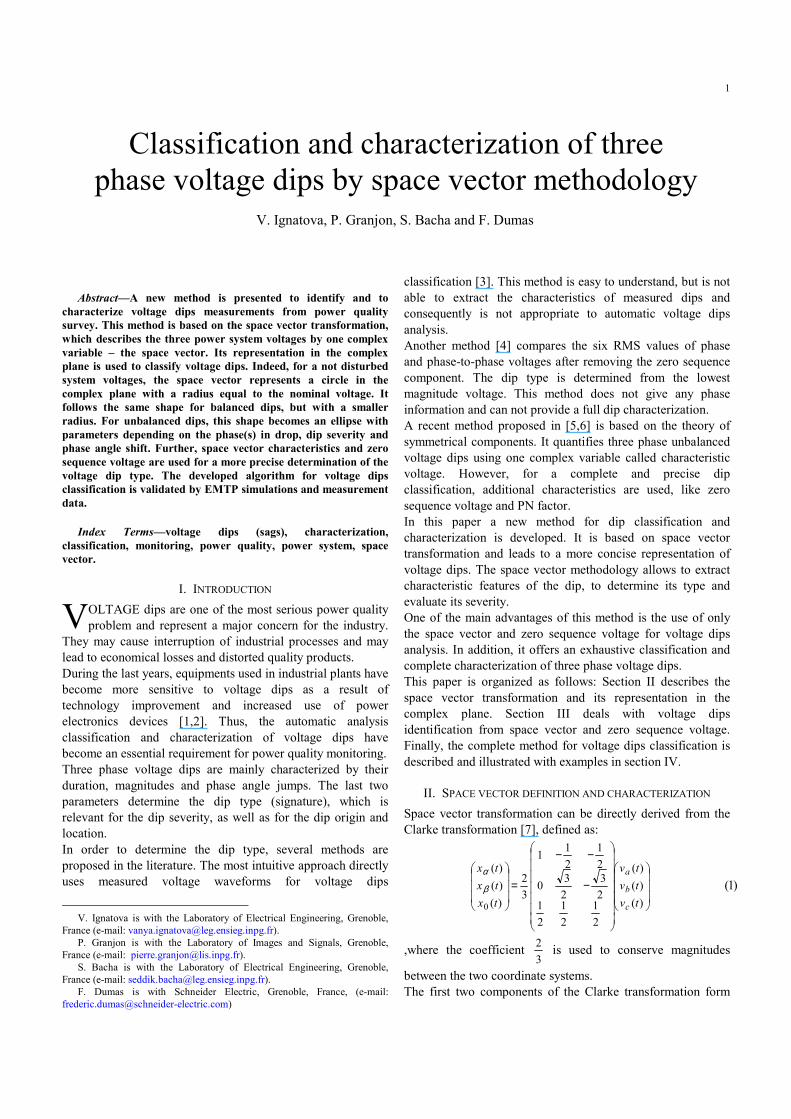
The space vector for the voltage dip represented in Fig.10 is

6

composed by a positive frequency phasor °−= 15878,0 jp ex and

a negative frequency phasor °= 381,0 jn ex . The shape index

76,0=SI classifies the dip as unbalanced. The ellipse

inclination °=120incϕ indicates that two phases are in drop: a

and c . The major ellipse axis 88,0max =r and the zero

sequence voltage 05,00 =x determine that the dip type is E.

The minor ellipse axis 67,0min =r indicates that the dip depth

is pud 33,0= .

Fig. 10 Double phase measured voltage dip

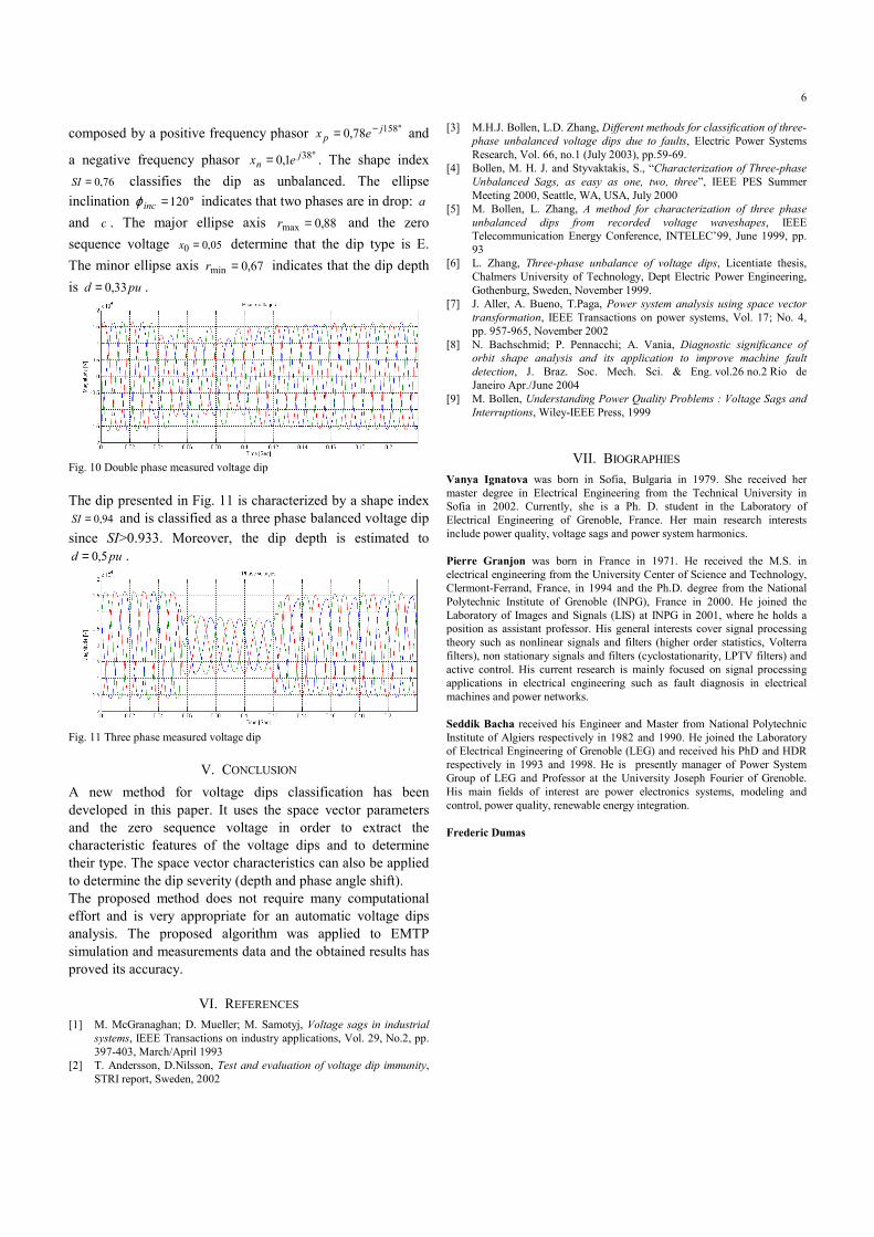
The dip presented in Fig. 11 is characterized by a shape index

94,0=SI and is classified as a three phase balanced voltage dip

since SI>0.933. Moreover, the dip depth is estimated to

pud 5,0= .

Fig. 11 Three phase measured voltage dip

V. CONCLUSION

A new method for voltage dips classification has been

developed in this paper. It uses the space vector parameters

and the zero sequence voltage in order to extract the

characteristic features of the voltage dips and to determine

their type. The space vector characteristics can also be applied

to determine the dip severity (depth and phase angle shift).

The proposed method does not require many computational

effort and is very appropriate for an automatic voltage dips

analysis. The proposed algorithm was applied to EMTP

simulation and measurements data and the obtained results has

proved its accuracy.

VI. REFERENCES

[1] M. McGranaghan; D. Mueller; M. Samotyj, Voltage sags in industrial

systems, IEEE Transactions on industry applications, Vol. 29, No.2, pp.

397-403, March/April 1993

[2] T. Andersson, D.Nilsson, Test and evaluation of voltage dip immunity,

STRI report, Sweden, 2002

[3] M.H.J. Bollen, L.D. Zhang, Different methods for classification of three-

phase unbalanced voltage dips due to faults, Electric Power Systems

Research, Vol. 66, no.1 (July 2003), pp.59-69.

[4] Bollen, M. H. J. and Styvaktakis, S., “Characterization of Three-phase

Unbalanced Sags, as easy as one, two, three”, IEEE PES Summer

Meeting 2000, Seattle, WA, USA, July 2000

[5] M. Bollen, L. Zhang, A method for characterization of three phase

unbalanced dips from recorded voltage waveshapes, IEEE

Telecommunication Energy Conference, INTELEC’99, June 1999, pp.

93

[6] L. Zhang, Three-phase unbalance of voltage dips, Licentiate thesis,

Chalmers University of Technology, Dept Electric Power Engineering,

Gothenburg, Sweden, November 1999.

[7] J. Aller, A. Bueno, T.Paga, Power system analysis using space vector

transformation, IEEE Transactions on power systems, Vol. 17; No. 4,

pp. 957-965, November 2002

[8] N. Bachschmid; P. Pennacchi; A. Vania, Diagnostic significance of

orbit shape analysis and its application to improve machine fault

detection, J. Braz. Soc. Mech. Sci. & Eng. vol.26 no.2 Rio de

Janeiro Apr./June 2004

[9] M. Bollen, Understanding Power Quality Problems : Voltage Sags and

Interruptions, Wiley-IEEE Press, 1999

VII. BIOGRAPHIES

Vanya Ignatova was born in Sofia, Bulgaria in 1979. She received her

master degree in Electrical Engineering from the Technical University in

Sofia in 2002. Currently, she is a Ph. D. student in the Laboratory of

Electrical Engineering of Grenoble, France. Her main research interests

include power quality, voltage sags and power system harmonics.

Pierre Granjon was born in France in 1971. He received the M.S. in

electrical engineering from the University Center of Science and Technology,

Clermont-Ferrand, France, in 1994 and the Ph.D. degree from the National

Polytechnic Institute of Grenoble (INPG), France in 2000. He joined the

Laboratory of Images and Signals (LIS) at INPG in 2001, where he holds a

position as assistant professor. His general interests cover signal processing

theory such as nonlinear signals and filters (higher order statistics, Volterra

filters), non stationary signals and filters (cyclostationarity, LPTV filters) and

active control. His current research is mainly focused on signal processing

applications in electrical engineering such as fault diagnosis in electrical

machines and power networks.

Seddik Bacha received his Engineer and Master from National Polytechnic

Institute of Algiers respectively in 1982 and 1990. He joined the Laboratory

of Electrical Engineering of Grenoble (LEG) and received his PhD and HDR

respectively in 1993 and 1998. He is presently manager of Power System

Group of LEG and Professor at the University Joseph Fourier of Grenoble.

His main fields of interest are power electronics systems, modeling and

control, power quality, renewable energy integration.

Frederic Dumas