Journal of Quantitative Analysis inSports

Volume 5, Issue 2 2009 Article 4

Chasing DiMaggio: Streaks in SimulatedSeasons Using Non-Constant At-Bats

David M. Rockoff∗ Philip A. Yates†

∗Iowa State University, drockoff@iastate.edu†California State Polytechnic University - Pomona, payates@csupomona.edu

Copyright c©2009 The Berkeley Electronic Press. All rights reserved.

Chasing DiMaggio: Streaks in SimulatedSeasons Using Non-Constant At-Bats∗

David M. Rockoff and Philip A. Yates

Abstract

On March 30, 2008, Samuel Arbesman and Steven Strogatz had their article “A Journey toBaseball’s Alternate Universe” published in The New York Times. They simulated baseball’s entirehistory 10,000 times to ask how likely it was for anyone in baseball history to achieve a streak thatis at least as long as Joe DiMaggio’s hitting streak of 56 in 1941. Arbesman and Strogatz treateda player’s at bats per game as a constant across all games in a season, which greatly overestimatesthe probability of long streaks. The simulations in this paper treated at-bats in a game as a randomvariable. For each player in each season, the number of at-bats for each simulated game was boot-strapped. The number of hits for player i in season j in game k is a binomial random variable withthe number of trials being equal to the number of at bats the player gets in game k and the prob-ability of success being equal to that player’s batting average for that season. The result of usingnon-constant at-bats in the simulation was a decrease in the percentage of the baseball historiesto see a hitting streak of at least 56 games from 42% (Arbesman and Strogatz) to approximately2.5%.

KEYWORDS: hitting streaks, simulations

∗The information used here was obtained free of charge and is copyrighted by Retrosheet.Interested parties may contact Retrosheet at 20 Sunset Road, Newark, DE 19711 or atwww.retrosheet.org. Thanks to Cliff Blau for DiMaggio’s 1941 game-by-game data.

1 BackgroundThe summer of 1941 was one of the most compelling times in baseball history. Thatyear, Ted Williams of the Boston Red Sox posted a batting average of .406 with37 home runs, 120 runs batted in, an on base percentage of .553, and a sluggingaverage of .735. He would be the last man to hit over .400 in a season. His leagueand park adjusted OPS (OPS+) was 235, the fourth highest mark of the twentiethcentury. This means that his OPS was 135% better than an average player in theAmerican League. All of these accomplishments earned Williams second placein the American League balloting for Most Valuable Player. The 1941 AmericanLeague MVP award went to New York Yankee Joe DiMaggio. DiMaggio hit .357with 30 home runs, 125 runs batted in, an on base percentage of .440, a sluggingaverage of .643, and an OPS+ of 184. However, DiMaggio had something thatWilliams did not: he hit safely in 56 straight games, a record that many say willnever be approached.

Due to the statistical anomaly that is DiMaggio’s hitting streak, there has beenmuch discussion and analysis about this feat. Gould (1989) wrote how “DiMag-gio’s streak is the most extraordinary thing that ever happened in American sports.”Short and Wasserman (1989) quantified the probability of streak similar to DiMag-gio’s with a conservative estimate of 3 at-bats per game. Berry (1991) comparedthe probabilities of DiMaggio’s 56 game hitting streak and Williams’ batting .406and found the two to be fairly comparable. Albright (1993) discussed ways of iden-tifying wide-scale streakiness in terms of hitting over a four year period. Warrack(1995) calculated the probability of DiMaggio having a 56-game hitting streak. Al-bert and Williamson (2001) simulated from a Bayesian model to measure a player’sstreakiness for hitting streaks and for home run streaks. Freiman (2002) attemptedto find the probability of a 56-game hitting streak by treating these streaks as beingnot independent. Albert (2008) used an exchangeable model to estimate hitting abil-ities of players, understand those players’ streakiness, and to identify some playerswho are streakier than others. Arbesman and Strogatz (2008) ran simulations ofbaseball seasons to estimate the probability of long hitting streaks, which resultedin a 56 (or more) game hitting streak in 42% of simulated baseball histories. Theytreated a player’s at-bats per game as constant across all games in a season.

This article will improve upon the results of Arbesman and Strogatz (2008).When they treated a player’s at-bats per game as constant across all games in aseason, they greatly overestimated the probability of long streaks. Varying the at-bats per game will not only better mimic the natural flow of a player’s season, butalso will reduce the estimated probability of a long hitting streak.

1

Rockoff and Yates: Chasing DiMaggio

Published by The Berkeley Electronic Press, 2009

2 ModelTo illustrate how constant at-bats can overestimate the likelihood of long hittingstreaks, Warrack (1995) estimates the probability of a player getting at least one hitin a game, p, in the following manner. Let pi be the probability that a batter withbatting average A comes to bat i times during a game. Then p can be estimated by

p̂ = ∑ pi(1− (1−A)i).

This function is concave in i. Let B be the average number of at-bats per game. Onecan estimate p by

p̂ = 1− (1−A)B.

One can make the argument that the first estimate of p is the expected value ofthe probability of a player getting at least one hit. The second estimate of p is theprobability of a player getting at least one hit over their average number of at-batsper game. By Jensen’s Inequality, the second p̂ is greater than or equal to the firstp̂. This means that using constant at-bats will overestimate the likelihood of longhitting streaks.

A brief example will be used to support this idea. Suppose a player’s battingaverage is .300, and over two games, the player has 8 total at-bats. The probabilityof getting a hit in both games is

p̂ ={

1− (1− .300)i}{1− (1− .300) j} ,

where i is the number of at-bats in the first game, j is the number of at-bats in thesecond game, and i+ j = 8.

Table 1 summarizes the probabilities in this example. The highest probabilityis the case where the player averaged 4 at-bats over the two games. Once theseat-bats are allowed to vary, the probability of getting at least one hit in both games(a two-game hitting streak) decreases. Low at bat games hurt the player’s chancesfor getting a hit in a game. Extended over long stretches, say a 162 game season,this effect is telescoped. Figure 1 further illustrates the need to vary at-bats whenanalyzing hitting streaks. Over time, the average number of at-bats per game hasdecreased.

2.1 The DataGame data was obtained from Retrosheet. For each season in their database, thisdata includes multitudes of information on every single plate appearance in themajor leagues, including unique game identifier, batter, and whether the appearance

2

Journal of Quantitative Analysis in Sports, Vol. 5 [2009], Iss. 2, Art. 4

http://www.bepress.com/jqas/vol5/iss2/4DOI: 10.2202/1559-0410.1167

Probability of HitIn Both Games

Game 1 Game 2AB AB

p̂

1 7 0.2752 6 0.4503 5 0.5474 4 0.5775 3 0.5476 2 0.4507 1 0.275

Table 1: Probability of a Player with a .300 Batting Average Getting a Hit in TwoGames with Eight Total at-bats

Figure 1: Boxplots of At-bats per Game Over All Baseball Seasons

3

Rockoff and Yates: Chasing DiMaggio

Published by The Berkeley Electronic Press, 2009

resulted in an at bat. This allows one to determine the number of at-bats of eachplayer in each game for each season. Retrosheet has game-by-game data for allof major league baseball from 1954− 2007, as well as for the National League in1911, 1921, 1922, and 1953.

2.2 The ModelFor hitter i in season j, the batting average is denoted as pi j. For example, the2000 and 2001 versions of a player like Barry Bonds will be treated as two differentplayers. If the ith hitter played in k games in season j, then

ABi j = (ABi j1,ABi j2, · · · ,ABi jk)

are the number of at-bats for each game over the course of the season. Assumingthat at-bats over the course of a single game are independent of each other, then thenumber of hits a player i in season j gets in game k, denoted Hi jk, has a binomialdistribution with n = ABi jk and p = pi j. This can be written as

Hi jk ∼ Bin(ABi jk, pi j).

R version 2.7.2 (2008) was used to run the simulations. In these simulations,each player in each season had their distribution of at-bats over the k games playedin a season. These at-bats were sampled with replacement to create a “simulated”season’s worth of at-bats. To use notation similar to Efron and Tibshirani (1993),the “simulated” season’s worth of at-bats are

AB∗i j = (AB∗i j1,AB∗i j2, · · · ,AB∗i jk).

If m seasons are simulated, then for player i and season j,

AB∗1i j ,AB∗2

i j , · · · ,AB∗mi j

represent that player’s “at-bats” in the simulations. The number of hits a player getsin each game in the mth simulated season is

H∗mi j ∼ Bin(AB∗m

i j , pi j).

After randomly generating base hits from this binomial distribution, a hitting streakwas considered to be any run of hits in H∗m

i j that are greater than zero. The simu-lations kept track of each player’s maximum hitting streak in any given simulatedseason.

4

Journal of Quantitative Analysis in Sports, Vol. 5 [2009], Iss. 2, Art. 4

http://www.bepress.com/jqas/vol5/iss2/4DOI: 10.2202/1559-0410.1167

Simulated SeasonPlayer Year 40+ 50+ 56+ Min Q1 Q2 Q3 MaxFelipe Alou 1966 4 3 2 9 14 16 21 75Julio Franco 1991 3 1 1 8 14 16 20 74Alex Rodriguez 1996 10 3 2 9 15 18 22 72Rogers Hornsby 1921 21 3 1 6 14 17 22 71Ichiro Suzuki 2004 34 8 5 11 18 22 27 69Jimmy Rollins 2007 2 1 1 7 13 15 18 64Rogers Hornsby 1922 23 4 2 7 15 18 23 63Ralph Garr 1974 13 3 2 9 15 18 22 63Kirby Puckett 1986 6 2 1 8 14 17 21 62Ichiro Suzkui 2007 14 2 1 10 16 19 23 61Rod Carew 1977 12 4 2 7 16 19 23 60Bobby Murcer 1973 1 1 1 5 11 13 15 60Luis Castillo 2002 2 1 1 7 12 14 17 58Wade Boggs 1985 10 2 1 9 16 19 23 57Larry Walker 1997 7 1 1 8 14 17 20 57Doug Glanville 1999 4 1 1 7 13 16 20 57Pete Rose 1975 1 1 1 8 13 15 18 57Tim Raines 1984 1 1 1 7 11 14 16 57Magglio Ordonez 2007 10 2 1 8 14 17 20 56Nellie Fox 1955 1 1 1 7 12 15 18 56Don Demeter 1962 1 1 1 6 10 12 14 56

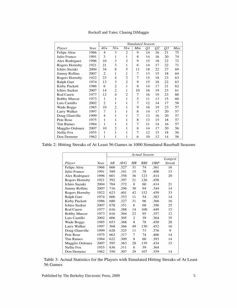
Table 2: Hitting Streaks of At Least 56 Games in 1000 Simulated Baseball Seasons

Actual SeasonLongest

Player Year AB AVG HR RBI OBP StreakFelipe Alou 1966 666 .327 31 74 .361 16Julio Franco 1991 589 .341 15 78 .408 15Alex Rodriguez 1996 601 .358 36 123 .414 20Rogers Hornsby 1921 592 .397 21 126 .458Ichiro Suzuki 2004 704 .372 8 60 .414 21Jimmy Rollins 2007 716 .296 30 94 .344 14Rogers Hornsby 1922 623 .401 42 152 .459 33Ralph Garr 1974 606 .353 11 54 .383 14Kirby Puckett 1986 680 .327 31 96 .366 16Ichiro Suzkui 2007 678 .351 6 68 .396 25Rod Carew 1977 616 .388 14 100 .449 15Bobby Murcer 1973 616 .304 22 95 .357 12Luis Castillo 2002 606 .305 2 39 .364 35Wade Boggs 1985 653 .368 8 78 .450 28Larry Walker 1997 568 .366 49 130 .452 16Doug Glanville 1999 628 .325 11 73 .376 9Pete Rose 1975 662 .317 7 74 .406 14Tim Raines 1984 622 .309 8 60 .393 14Magglio Ordonez 2007 595 .363 28 139 .434 15Nellie Fox 1955 636 .311 6 59 .364Don Demeter 1962 550 .307 29 107 .359 14

Table 3: Actual Statistics for the Players with Simulated Hitting Streaks of At Least56 Games

5

Rockoff and Yates: Chasing DiMaggio

Published by The Berkeley Electronic Press, 2009

Method Max 40+ 50+ 56+Constant AB 75 57 8 2Variable AB 57 41 2 1

Table 4: 10,000 Simulations of DiMaggio’s 1941 Season

3 Simulation & ResultsUsing the data obtained from Retrosheet’s game logs, 1000 baseball “histories”were run in R. Technically, these are half-histories because very little of the datais for games prior to 1953. Since we have 58 seasons worth of data, and eachseason was simulated 1000 times, there are 58,000 simulated seasons. DiMaggio’srecord 56-game hitting streak was matched or exceeded in 30 of them, or 0.00517%.Table 2 lists the players who achieved this feat in the simulations; table 3 lists thoseplayers’ actual statistics.

Felipe Alou had the longest streak, 75 games in the simulated 1966 season.Ichiro Suzuki is the player appearing most often among these record streaks. Hissimulated 2004 seasons included 5 record-breakers, meaning that he had a 1-in-200 chance of breaking the record that year. He also broke the record once in thesimulated 2007 season.

Twenty five of the simulated half-histories, or 2.5%, contained at least onestreak of 56 games, meaning that there was a 2.5% chance that there would actuallyhave been such a streak in the past 58 years.

As an explicit comparison of the variable at-bat model with the constant at-bat model, 10,000 simulations of Joe DiMaggio’s 1941 season were run for eachmodel. Table 4 shows for each model the maximum streak, the number of seasonswith a streak of at least 40 games, the number of seasons with a streak of at least 50games, and the number of seasons with a streak of at least 56 games. The constantat-bat model resulted in greater numbers all around, confirming that long streaksare more rare under the variable at-bat model.

4 Summary & ConclusionsIdeally, simulations would be run on the entire history of baseball. However, for thetime being, Retrosheet game-by-game data goes back essentially to 1953. Thus theresults presented here are not directly comparable to those obtained by Arbesmanand Strogatz, who frame their simulations mainly in terms of baseball histories.

It may be possible to use known (1953 and after) game-by-game at-bat distri-

6

Journal of Quantitative Analysis in Sports, Vol. 5 [2009], Iss. 2, Art. 4

http://www.bepress.com/jqas/vol5/iss2/4DOI: 10.2202/1559-0410.1167

butions to model unknown (before 1953) at-bat distributions based solely on aver-age at-bats per game. It was hoped that players’ game-by-game at-bats would fol-low a “nice” distribution, such as Poisson with mean parameter equal to a player’saverage at-bats per game during the season, represented in statistical terms as

ABi jk ∼ Poi(

ABi j

Gi j

).

Thus far, all such models examined have proven to be poor fits to the actual data.A somewhat more complex method to model a player’s unknown at-bat distri-

bution would be to use a player with a known at-bat distribution and the same seasonaverage at-bats per game. As a simplistic example, if players with 4.0 at-bats pergame in a season tend to have 3 at-bats in one-third of their games , 4 at-bats inone-third of their games, and 5 at-bats in the remaining one-third of their games,that same distribution could be applied to pre-1953 players who had 4.0 at-bats pergame.

Another way in which the simulations may be modified is by treating a player’sbatting average as a random variable that changes from game to game or at-batto at-bat, rather than remaining constant throughout the season. Some promisingcandidates are the beta and the normal distributions, with mean equal to the player’sactual season batting average.

Lastly, some limitations of the research discussed in this article ought to betaken into account. For one, these simulations did not take into account certainreal-life baseball decisions that may factor into a player’s at-bats during a hittingstreak. For instance, a player in the midst of a lengthy streak is unlikely to bepulled by the manager in the middle of the game if he has not yet gotten a hit in thegame. Similarly, such a player may be less likely to “settle” for a base-on-balls if astreak is on the line. In the simulations, if a player has a sizeable streak going andis randomly assigned a two at-bat game, that’s his tough simulated luck.

Furthermore, since the simulations only capture each player’s longest streak ineach simulated season, they do not account for the remote possibility of multiplelong streaks by a player in a given simulated season. Similarly, the results do notcapture multi-season streaks such as the one Jimmy Rollins had (in real life) at theend of 2005 and the beginning of 2006.

7

Rockoff and Yates: Chasing DiMaggio

Published by The Berkeley Electronic Press, 2009

Albert, J., & Williamson, P. (2001). Using Model/Data Simulations to DetectStreakiness. The American Statistician, 55(1), 41–50.

Albright, S. C. (1993). A Statistical Analysis of Hitting Streaks in Baseball. Journalof the American Statistical Association, 88(424), 1175–1183.

Arbesman, S., & Strogatz, S. (2008 March 30). A Journey to Baseball’s Al-ternate Universe. The New York Times. (Retrieved: 2008 March 31;http://www.nytimes.com/2008/03/30/opinion/30strogatz.html)

Berry, S. (1991). The Summer of ’41: A Probability Analysis of DiMaggio’s Streakand Williams’ Average of .406. Chance, 4(4), 8–11.

Efron, B., & Tibshirani, R. J. (1993). An Introduction to the Bootstrap. Boca Raton:Chapman & Hall/CRC.

Freiman, M. (2002). 56-Game Hitting Streaks Revisited. The Baseball ResearchJournal, 31, 11–15.

Gould, S. J. (1989). The Streak of Streaks. Chance, 2(2), 10–16.R Development Core Team. (2008). R: A Language and Environment for Sta-

tistical Computing. Vienna, Austria. (ISBN 3-900051-07-0; http://www.R-project.org)

Short, T., & Wasserman, L. (1989). Should We Be Surprised by the Streak ofStreaks? Chance, 2(2), 13.

Warrack, G. (1995). The Great Streak. Chance, 8(3), 41–43, 60.

ReferencesAlbert, J. (2008). Streaky Hitting in Baseball. Journal of Quantitative Analysis in

Sports, 4(1), Article 3.

8

Journal of Quantitative Analysis in Sports, Vol. 5 [2009], Iss. 2, Art. 4

http://www.bepress.com/jqas/vol5/iss2/4DOI: 10.2202/1559-0410.1167