Controlled versus Continuous Calving Seasons in the South: What's at Stake

Controlled versus Continuous Calving Seasons in the South:What’s at Stake?

By Damona Doye, Michael Popp, and Chuck West

IntroductionAnimal scientists have long encouraged producers to adopt controlled breeding seasons

in their cow/calf herds. For example, as part of the Arkansas Beef Improvement

Program (ABIP), special projects were developed to address common beef management

problem areas, including establishing breeding and calving seasons (Troxel et al., 2004).

Hopkins, Neel, and Blair advocate a controlled calving season for top reproductive

performance. In the Oklahoma Beef Cattle Manual, Selk and Barnes state that the use

of two defined calving seasons may allow producers to reduce bull costs, allow fall-born

heifers to be bred in spring (and spring born heifers to be bred in fall) to calve at more

than two years of age, and spread marketing risk.

However, evidence persists that the recommendation to develop either one or two

controlled breeding seasons has been ignored by many producers. 1997 National

Animal Health Monitoring Systems (NAHMS) data indicated that nearly 54 percent of

operations have no set calving season. Recent data collected with the distribution of

Oklahoma beef cattle manuals indicated that 47 percent of producers with fewer than

100 cows and less than 40 percent of household income from the beef enterprise leave

the bull out year-round (Vestal, Ward, Doye & P, 2006). Hypothetical reasons for this

phenomenon vary. One reason given by producers relates to cash flow.

2008 JOURNAL OF THE A|S|F|M|R|A

60

Abstract

This paper analyzed the financialramifications of differences inseasonal input requirements of cow-calf operations by comparing adefined 90-day calving season toyear-round calving. Assuming thesame calving rate and laborrequirements for both productionsystems, as well as no premiums forlarger, more uniform lots of calveswith the controlled calving season,uncontrolled calving resulted inslightly higher returns primarily dueto better seasonal forage utilization.However, minimal changes tocalving rate, expected calf pricepremiums, and changes in laborrequirements favored controlledcalving with returns deemedinsufficient for small operators toswitch from their current practice.

Damona Doye is an extension economist and Regents Professor in the Department ofAgricultural Economics at Oklahoma State University.

Michael P. Popp is Professor in the Department of Agricultural Economics andAgribusiness at the University of Arkansas.

Charles P. West is Professor in the Department of Crop, Soil, and EnvironmentalSciences at the University of Arkansas.

Damona Doye and Michael Popp share lead authorship of this article.

In any given month, a calf could be ready for sale, thus

enabling timely payment of either expected or unexpected

expenses. An income-averaging rationale is also sometimes

offered, suggesting that because calf sales are scattered

throughout the year, producers are guaranteed not to sell the

entire calf crop at the year’s lowest price. Further, an

uncontrolled breeding system is “easy;” for example, bulls do

not have to be maintained separately. Another reason proffered

is that forages may be better utilized.

Specialists who recommend controlled breeding seasons note

that benefits include the ability to better manage cow nutrition,

cow and calf health, cow culling, weaning programs, and

marketing of calves and cull cows. With a continuous calving

system, a herd always consists of cows in different stages of

lactation and/or gestation with attendant-varying nutritional

requirements. Thus, with uncontrolled calving, if the herd is

fed to meet the needs of the lactating cow(s), the average cow

may be overfed resulting in feed costs that are higher than is

necessary; alternatively, if nutrition is not balanced, the

lactating cow is malnourished leading eventually to lesser beef

production. Similarly, the potential of seasonal income

averaging and cashflow benefits of a continuous calving system

may be more than offset by failure to capture price premiums

for consistent, larger batches of calves that may be sold if the

calving season is controlled and calves are sold once per year

(Avent, Ward, & Lalman, 2004; Troxel et al., 2006).

Therefore, questions regarding real or perceived economic

benefits are important since the decision to modify calving

season typically involves major adjustments in management

over several years. For the five farms enrolled in the ABIP

project for example, it took an average of 4.3 +/- 0.58 years to

reach desired breeding and calving season goals (Troxel et al.,

2004). Over the course of the project, the percentage of cows

calving in the desired calving season increased from 36.5

percent in the baseline year to 100 percent within 5 years. The

authors indicated that specified costs per animal unit decreased

and that income over specified costs improved, demonstrating

that defining the breeding season increased beef production

efficiency in this case.

The objective of this study was to analyze the impact of

potential factors affecting the adoption of a controlled breeding

system. The financial impact of differences in calving season

management on cattle and forage enterprises was assessed and

sensitivity of results to assumptions on calving rate (with

attendant cow nutrition requirements and forage utilization),

operator labor requirements, and calf sale prices were tested.

This was done to test a null hypothesis of insignificant

differences in financial performance of cow-calf operations

using a defined 90-day spring calving season similar to

Anderson et al. versus a production system where reproductive

performance is more or less a function of seasonal pasture

production and natural breeding seasons. Additional analyses

were also performed to examine differences in economic returns

related to pasture type to provide producers and extension

agents further information about calving season management.

BackgroundLivestock budget studies are periodically conducted in many

geographic regions, typically with either a stocker or cow/calf

focus and often with specific forage-base and management

assumptions (Walker, Lusby & McMurphy, 1987; Zaragoza-

Ramire, Bransby, & Duffy, 2006; Phillips et al., 2003; National

Ag Risk Education Library, 2006; King-Brister, 2003).

Production budgets for beef cattle and pastures may spell out

cow herd dynamics, nutrient requirements, medical expenses,

labor requirements, machinery and equipment operating costs,

overhead costs, and other costs along with production and sales

data. These budgets allow producers to evaluate the potential

returns to land, management, and capital resources of pasture-

based cow/calf production systems. Decision support tools for

ranchers also often focus on potential production or economic

outcomes in fairly narrowly defined scenarios, for instance, cost

and returns associated with a specific size of operation.

Research to identify the most profitable enterprises for a given

resource base in a systems framework that incorporates forage

production details and livestock nutritional requirements is

scarce, however. May, Van Tassell, Smith and Waggoner used

integer programming to examine optimal monthly feeding

strategies and costs for March and May calving alternatives

(1998), and to identify minimum cow feed costs with basin wild

rye as a winter grazing option (1999). Smith et al.’s mixed

integer programming model used both quality and quantity

measures of forage in matching seasonal forage production and

livestock nutritional requirements to solve for optimal


61

combinations of cow/calf and stocker enterprises on different

resource bases.

Data and MethodsAnimal unit months (AUMs) have traditionally been used to

define the carrying capacity of pasture. But, the quantity

produced and quality of different forages vary significantly over

a year, and different calving season patterns place different

seasonal demands on forages, labor, and capital, for example.

Thus, a model able to incorporate seasonality of inputs and

outputs and solve for optimal solutions under different

conditions was needed. The modeling framework of Smith

(1999) was adapted to a base case scenario of a small 50-cow

operation in Arkansas to determine the conditions under which

a producer might elect to control their cow breeding and hence

calving season.

The model solves for the optimal combination of forage and

beef production to maximize returns to an operator’s land

resource base, labor, management and risk and can be

mathematically described as:

where:

Cj = income or costs of activity jXj = level of activity j

subject to the constraints:

where:

aij = quantity of resource i required per unit of activity jbi = quantity of resource i

The linear programming tableau was built in Microsoft Excel.

The tableau referred to other worksheets in the spreadsheets that

contained data, formulas for calculations, and user-entered

information regarding resources and production preferences.

Potential production activities included cow-calf, stocker, crop,

and forage enterprises. For this research, the activities were

restricted to cow-calf and forage enterprises. As the tableau for

this model exceeded the limits for the standard Excel Solver,

Solver Premium Plus from Frontline Systems was used. Linear

programming was used to solve the continuous model through

several iterations of simultaneous equations.

The total number of owned acres by land type, the minimum

and maximum number of acres of crop and forage enterprises,

and the expected annual production per acre (including forage

quality) for each type of forage used were specified. Cow-calf

nutrient requirements were a function of average body weight

(BW) of cows in the herd, average body condition score for

cows, average cow milk production, average expected calf birth

weight, expected percent calf crop, expected percent of

replacement heifers, and expected calf weaning weights

(National Research Council [NRC]). Cow-calf nutritional

requirements were calculated for various stages of the

reproductive cycle (first 180 days, following 90 days, and last

90 days). Maximum dry matter intake (DMI) of cows was set

to 2.5 percent and minimum consumption to 1.5 percent of BW

(NRC, 1984). For every pound of dry matter (DM) used by the

animals, associated pounds of crude protein (CP) and total

digestible nutrient (TDN) were also used.

Monthly forage quality was characterized by TDN, CP, and DM

quantity, with the quantity produced and quality of different

forages varying significantly during a year. Stockpiling of

forage resulted in decreased available quality and quantity over

time and was dependent on forage type. Both forage quality

and quantity adjustments for stockpiled forage were based on

expert opinion (West, 2006) and forage transfer from month to

month ranged from 68-75 percent depending on climatic

conditions. Forages could also be harvested for hay in summer

months if not used by the animals. The model was not sensitive

to grazing intensity, nor was an animal’s DMI a function of

TDN concentration in the diet. However, because the model

selected forages to meet livestock DM requirements and the

TDN values varied by forage type and by month, the TDN

concentration of the diet was unknown before the model was

run. Therefore, if CP or TDN requirements were a limiting

factor for the animal’s nutrition in any month, hay and/or other

supplemental nutrition could be produced on farm or purchased.


62

Monthly labor requirements, operating capital, and total costs

(excluding labor, feed, and capital costs) for all forage, crop,

and livestock enterprises were specified along with general farm

information, such as starting operating capital, maximum capital

that can be borrowed, annual percentage rate on the borrowed

capital, monthly labor hours available from the owner/operator,

and the wage rate for hired labor. If labor was a limiting factor

in any month, additional labor could be hired up to a user-

specified limit.

In this application of the model, farm income was generated

from the sale of hay or calves. The calf crop was assumed to be

half bull calves and half heifers. An output worksheet

summarized the number of spring calving and continuous

calving cows, the number of head of steer and heifers calves

sold, and supplemental hay and feed purchases by month. A

labor summary table showed the number of owner/operator

hours used, number of hired labor hours purchased, cost of

hired labor per hour, and total cost of hired labor. Total capital

required, own capital provided, operating capital borrowed, and

interest on capital were also tabulated. Finally, monthly sales

and expenses along with net returns to land, overhead, own

labor, and capital can be analyzed.

For sensitivity analyses, specific parameters that were expected

to differ under controlled and uncontrolled breeding season

production systems were modified, including 1) calving rate,

defined as ratio of the number of calves sold to the number of

cows exposed to a herd sire on an annual basis; 2) operator

labor requirements for performing not only physical but also

management operations associated with the cow-calf enterprise;

and 3) calf prices net of marketing charges to account for

potential price premiums for larger and more consistent batches

of calves. Finally, the impact of changing to more intensive

pasture management was also considered to test for owner labor

and land cow-carrying capacity limitations. That is, a producer

changes pasture management and then the model tests whether

continuous or controlled calving leads to optimal returns.

Beyond the scope of this study were interactions between

pasture management by calving season management. For

instance, it may be argued that a producer using an uncontrolled

calving season would likely also manage his or her pastures less

intensely, but this aspect was not modeled here.

Base Case ScenarioArkansas forage information and beef production practices were

updated using existing production budgets (King-Brister, 2003).

Two types of pasture were available to the operator. A less

intensive pasture management choice was well managed,

existing Bermuda and fescue pastures yielding forage

production of 9,250 lb. of DM per acre; an alternative was a

more labor and capital intensive system requiring sod seeding

rye for winter annual forage. With winter rye production, total

annual forage production increased to 15,800 lb. of DM per

acre with heightened potential for early season grazing in

February and March. This is accomplished by sod seeding rye

in September of the previous year. Due to rolling terrain as

well as soil limitations, only limited acreage was available for

sod seeding for the base case. Finally, given forage

establishment difficulties, pasture fertilization was assumed to

maintain these pastures and thereby obviated the need to

reestablish pastures and associated establishment charges.

Figure 1 shows the differences in weighted average DM

production (top panel), forage CP (middle panel), and TDN

content (bottom panel) for the two pasture types. Note that a

base of 50/50 Bermuda and Fescue grasses were assumed with

average production and quality parameters quantity weighted by

month with the exception of January where stockpiling was

assumed. In the model, grazing efficiency for forage was

assumed to be 35 percent for both pasture types and calving

scenarios. Unused forage could be baled at a cost of $40/ton

and sold at $60/ton at a harvest efficiency of 70 percent. Again,

this assumed that both controlled and continuous calving

producers managed their pastures intensively and in a similar

fashion.

Product prices and operating costs were entered for each

enterprise, as were labor requirements by month (Tables 1-3).

The model calculated operating capital requirements, operating

interest, and returns to management, labor, and capital as no

ownership charges were assessed. Thus model solutions

represent a steady-state solution to owned resources. Maxima

on borrowed capital were set at $200,000 with an interest rate

of 6 percent APR. Available owner/operator hours were

specified by month with a constraint of 100 hours per month;

similarly, a maximum number of 100 hired labor hours per

month was specified at $8.00 per hour.


63

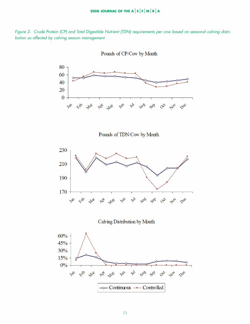
The distribution of calving for the continuous calving system

was based on observations with producers beginning the ABIP

program (Richeson, 2006). Compared to the spring calving

cows with a defined 90-day calving season from January to

March, the continuous calving system more evenly spreads out

nutritional requirements (Figure 2). For either controlled or

continuous calving cow/calf production, average cow weight

(1,100 lb), body condition score (5), milk production (11

lbs/day), calf birth weight (90 lb), percent calf crop (90), and

weaning weights for steers (550 lbs.) and heifers (525 lbs.) were

equal in the base case scenario. Livestock nutritional

requirements were met with pasture and, if needed, hay

produced on farm or purchased. Hay quality ranged from lower

quality, average Arkansas mixed hay at a cost of $60/ton

delivered (11% CP, 52% TDN, and 13% DM) or higher quality,

Arkansas Timothy hay harvested in its late vegetative stage at

$80/ton delivered (14% CP, 62% TDN, and 11% DM)

(Gadberry, 2006). Supplements, 20 or 38 percent CP range

cubes, could also be purchased at a price of $0.137 and $0.172

per pound respectively.

Seasonal calf sale prices were based on 1998-2007, long term,

nominal, average Arkansas monthly prices (USDA – AMS,

2008) to avoid basing the analysis on cyclically high or low

market prices. For both systems, quantity-weighted average

monthly prices were used in the model for steer and heifer calf

sales. That is, calves were sold seven months after weaning at

the average market price associated with that month of the year.

This resulted in an average, quantity weighted, seasonally

adjusted price of $97.29 and $98.55 per cwt for steers and

$89.73 and $90.66 for heifers, respectively, for the controlled

compared to the continuous systems. The cash flow month for

sales was associated with the modal calving month to simplify

cash flow modeling (February calving and September cash flow

for both systems). Finally, the above prices did not include

marketing charges of $6 per head for hauling and $15 per head

for sales commission and insurance. This allowed for

appropriate sensitivity analyses on calf price premiums and

calving rate as impacts of per head charges would not be mixed

with price changes. Pecuniary economies of size in marketing

calves were considered indirectly as larger, more uniform lots

may also reap lower transport costs (i.e., part of the price

premium could be transport cost efficiencies).

Cow replacements were assumed to be cost-neutral in the sense

that foregone heifer calf sales and replacement heifer feeding

costs were offset by cull cow sales either as cow/calf pairs or as

open cull cows. This is somewhat restrictive (Feuz, 2006) but

model size limitations dictated this restriction.

ResultsSince most beef cattle operations in Arkansas have fewer then

50 head (USDA – NASS), an initial run of the model was used

to determine the acreage needed to meet the nutritional needs of

a 50 cow herd. Results indicated that approximately 40 acres of

the Bermuda/fescue pasture as well as 20 acres of the sod-

seeded pasture were needed to primarily pasture feed

approximately 50 cows and supplementing with purchased hay

during the winter months. This solution conforms well to

pasture acreage requirements observed in Arkansas. Initially,

the two cow-calf enterprises were assumed to be similar in

terms of total non-nutrition costs and labor requirements with

cost and revenue changes primarily a function of differences in

seasonal calving distribution and associated monthly cow/calf

nutrition requirements.

The differences between the two systems in returns as well as

annual levels of key inputs were small given the initial

assumptions.1 Controlling the breeding season resulted in

slightly lower returns for the herd as slightly more purchased

hay was required. Examination of key production variables by

month however, pointed out two things. One, as the nutritional

needs for a spring-calving herd are greater than or equal to the

need in a continuous calving herd for January through June,

winter and early spring forage availability is critical and

therefore conditions that would allow for more sod seeding

would be preferred with controlled calving. Two, controlling

the breeding season placed a much higher demand on operator

labor in February and March. If less than 100 hours of operator

labor were available or off-farm jobs prevented extra hours in

these months, as may be the case for some small operations,

producers may choose to spread the calving season out over the

year to more easily meet their labor constraints.

Sensitivity analysis showed the financial ramifications of

changes in model assumptions for calving rate, calf sale prices,

labor requirements, and pasture availability. An argument can

be made that the calving rate for continuous calving operations


64

is typically lower than that of operations with controlled

breeding seasons as the herd’s nutritional needs at different

gestational stages may be better targeted, e.g., open cows are

more obvious and culled. ABIP records showed a disadvantage

of approximately one percent lower calving rate for continuous

compared to controlled calving operations (J. Richeson,

personal communication, March 2006). Not surprisingly, given

the small differences shown in initial runs, a reduction in

calving rate from the 90 percent base case scenario to 88.5

percent causes a switch from continuous to controlled calving

(Table 4). Results are also highly sensitive to calf prices. A

$1.10 per cwt price premium for calves from a controlled

breeding season resulting from larger, more uniform calf groups

or pecuniary economies of size in transport caused controlled to

be selected over the continuous breeding enterprise (Table 4).

For the base case scenario, total annual labor requirements per

cow were assumed to be equal for the continuous calving

system and year round calving as no studies document which

system requires more operator time. We argue that controlling

calving will save labor hours by not having to constantly

monitor calving (continuous calving operations may require a

somewhat constant need for cattle monitoring as cows could be

calving in any month), but may also lead to more labor hours

for more cattle handling for pregnancy checks, cattle sorting

and record keeping.

A “most likely” scenario for differences between the two

production systems was therefore developed which included an

85 percent calf crop for continuous calving operations

(compared to 90% for controlled calving seasons), a 25 percent

higher labor requirement for controlled calving enterprises, and

a $3 per cwt price premium and/or equivalent in transport

savings for calves from the controlled breeding season. In this

case, the controlled breeding season enterprise prevails despite

higher labor requirements because of the difference in sales

generated by more calves at higher prices. Table 4 shows the

resulting changes in key variables. Alternative pasture

scenarios were also analyzed to determine the land base’s

impact on the type and scale of operation. Sixty acres with no

sod-seeded pasture reduced cow-carrying capacity and

significantly reduced net returns but eliminated the need for

hired labor. A shift to a greater proportion of sod-seeded

pasture allowed for herd expansion and increased returns but

required additional hired labor.

Conclusions and RecommendationsDifferent model runs compared net returns to land, owner labor

and capital plus annual labor requirements, amount of hay fed,

cow carrying capacity, calf sales, annual operating interest, and

associated capital requirements to identify under what

conditions producers would choose among continuous or

controlled calving seasons. With continuous and controlled

calving assumed to have similar labor requirements and calving

rate, the initial solution, using Arkansas farm size and forage

conditions, narrowly favored continuous calving. A controlled

breeding season with spring calving resulted in high demands

for forage at a time when production is negligible or low.

Results also show, perhaps more importantly, that available

owner labor in small, part-time operations may be stressed with

controlled calving. For these reasons, continuous calving did

not and does not seem unreasonable in some circumstances.

Thus, educators and farm managers need to be cognizant of the

constraint that operator labor may place on recommendations

made.

Sensitivity analyses revealed that even small changes in

assumptions favoring controlled breeding seasons make control

over breeding season the more profitable choice. Either a 1.5

percent advantage in calving rate or a $1.10 per cwt premium

for larger, more uniform calf lots sold shifted the choice to the

controlled breeding enterprise. Further, a combination of price

premiums and higher calving percentages outweighed higher

labor requirements for the controlled calving season, even if

additional labor needed to be hired. Thus, our results suggest

that small producers may benefit from a variety of educational

programs with economic content, particularly studies showing

price premiums associated with marketing calves in uniform

groups, and analyses that demonstrate the importance of calving

rate in determining financial returns.

Additional research is needed to quantify differences in key

statistics, such as calving percentage and labor use for typical

operators employing continuous breeding systems relative to

those using controlled breeding systems. Finally, further study

related to pasture management in combination with calving

season management is expected to highlight additional labor

and/or production cost differences across systems.


65

References

Anderson, L.K. (1998, June). Ball, D.M. Blaylock, R.E., Floyd, J.G., Gimenez, D.M., Jones, W.R., Prevatt, J.W., & VanDyke, J.,

contributing authors. Reproductive Management – Key to Success: Control of Reproduction. Alabama Beef Cattle ProducersGuide. ANR-1100.

Avent, R.K., Ward, C.E., & Lalman, D. L. (2004). Market Valuation of Preconditioning Feeder Calves. Journal of Agricultural andApplied Economics, 36, 1, :173-183.

Feuz, D. (2006). The Costs of Raising Replacement Heifers and The Value of a Purchased vs. Raised Replacement. Retrieved July

10, 2006, from http://www.lmic.info/tac/other/Otherframe.html.

Gadberry, S. (2006). Composition of Some Livestock Feeds. Retrieved July 10, 2006, from

http://www.uaex.edu/Other_Areas/publications/ PDF/FSA-3043.pdf.

Hopkins, F., Neel, J.B., & Blair, R. (2004). Reproductive Management of Cow-Calf Operations. Tennessee Master Beef ProducerManual. The University of Tennessee. PB1722.

King-Brister, S. (2003). Budgeting Arkansas Beef Cattle Performance Through Alternative Marketing and Production Strategies.

Unpublished M.S. thesis, University of Arkansas.

May, G.J., Van Tassell, L.W., Smith, M.A., Waggoner, J.W. (1998, August 2-5). Optimal Feed Cost Strategies Associated with Earlyand Late Calving Seasons. American Agricultural Economics Association Paper.

May, G.J., Van Tassell, L.W., Smith, M.A., & Waggoner, J.W. (1999, July 11-14). Profitability of Establishing Basin Wildrye for

Winter Grazing. Western Agricultural Economics Association Paper.

National Ag Risk Education Library. (2006). Budget Library. Retrieved March 15, 2006, from

http://www.agrisk.umn.edu/Budgets/CustomSearch.aspx.

National Animal Health Monitoring Systems. (1997). Reference of 1997 Beef Cow-Calf Management Practices, Part I. Fort

Collins, Colorado: NAHMS.

National Research Council. (1984). Nutrient requirements of beef cattle, 6th Ed. Washington, D.C.: National Academy Press.

Phillips, W.A., Northup, B.K., Mayeux, H.S., & Daniel, J.A. (2003). Performance and Economic Returns of Stocker Cattle on

Tallgrass Prairie Under Different Grazing Management Strategies. The Professional Animal Scientist, 19, 416-423.

Richeson, J. Personal Communication. University of Arkansas, Animal Science, Cooperative Extension Service. March 2006.

Selk, G. & Barnes, K. (2005, August). Choosing a Calving Season. Beef Cattle Manual, 5th ed. (D. Doye & D. Lalman, Eds.).

Stillwater, OK: Oklahoma Cooperative Extension Service, Oklahoma State University.


66

Smith, K. E. (1999). Optimizing Forage Programs for Oklahoma Beef Production. Unpublished M.S. Thesis, Oklahoma State

University.

Smith, K.E., Kletke, D., Epplin, F., Doye, D., & Lalman, D. (2000, February). Optimizing Forage Programs for Oklahoma BeefProduction. SAEA Paper.

Troxel, T.R., Gadberry, M.S., Jenning, J.A., Kratz, D.E., Davis, G.V., & Wallace, W.T. (2004). Arkansas Beef Improvement

Program – An Integrated Resource Management Program for Cattle Producers. The Professional Animal Scientist, 20, 1-14.

Troxel, T.R., Barham, B. L., Cline, S., Foley, J., Hardgrave, D., Wiedower, R., & Wiedower, W. (2006). Management Factors

Affecting Selling Prices of Arkansas Beef Calves. Journal of Animal Science (Suppl. 1), 84, 12.

USDA, Agricultural Marketing Service (AMS). (2006). Livestock and Market News.

USDA, National Agricultural Statistics Service (NASS). Cattle. Retrieved July 10, 2006, from

http://jan.mannlib.cornell.edu/reports/nassr/livestock/pct-bb/catl0103.pdf.

Vestal, M.K., Ward, C.E., Doye, D.G., & Lalman, D.L. (2006). Beef Cattle Production and Management Practices and Implications

for Educators. SAAEA Paper.

Walker, O.L., Lusby, K.S., & McMurphy, W.E. (1987, February). Beef and Pasture Systems for Oklahoma: A BusinessManagement Manual. Oklahoma Agricultural Experiment Station Research Project P-888.

West, C. Personal Communication. University of Arkansas, Department of Crop Soil and Environmental Sciences. June, 2006.

Zaragoza-Ramire, J., Bransby, D.I., & Duffy, P. A. (2006, February). Economic Returns to Different Stocking Rates for Cattle on

Ryegrass under Contract Grazing and Traditional Ownership. SAEA Paper.

Endnote

1 Information on monthly, key production statistics like labor use, capital requirements, minimum DM intake, grazing

consumption, and hay purchases are available from the authors upon request.


67


68

Table 1. Estimated costs excluding operating interest per acre, maintaining established fescue, and bermuda grass forgrazing in Arkansas, 2008

1 It is unlikely that a producer would spend this amount of money on fertilizer. Alternatives such as overseeding nitrogenfixing legumes like clover, birdsfoot trefoil or lespedeza or application of poultry litter are more likely. The above arenonetheless recommended fertilization practices and therefore the reader is cautioned that the above cost estimatesare likely conservatively high.

2 With the fertilizer purchase, a buggy is supplied at no extra charge for use with the 50 hp tractor. Each applicationrequires 0.15 hrs/acre of labor and the September application is one trip for both fertilizers.


69

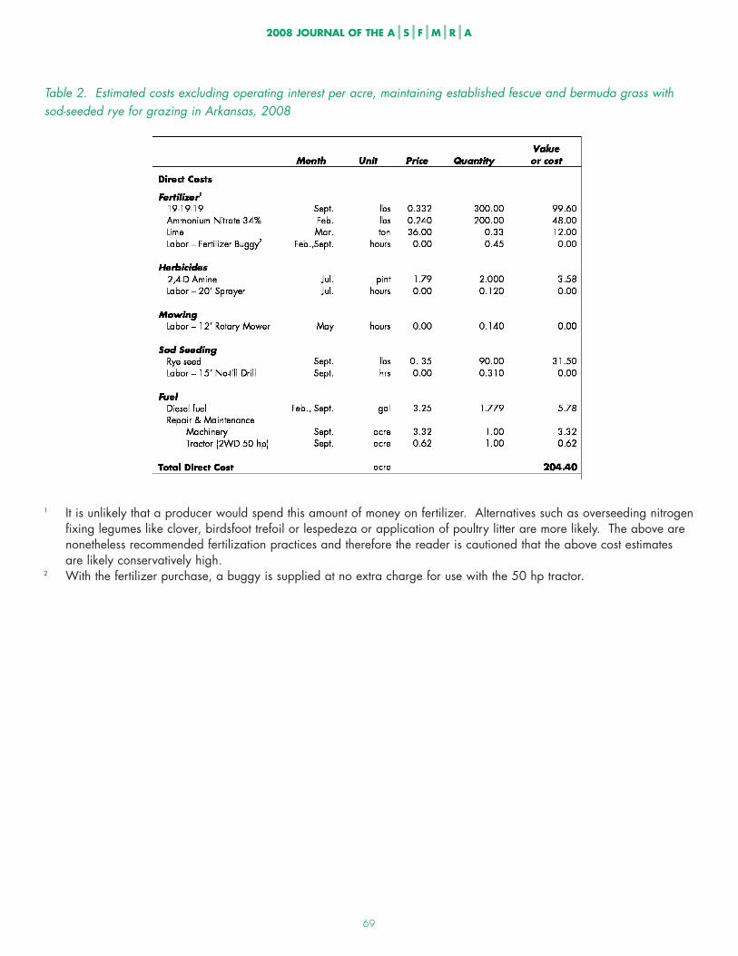
Table 2. Estimated costs excluding operating interest per acre, maintaining established fescue and bermuda grass withsod-seeded rye for grazing in Arkansas, 2008

1 It is unlikely that a producer would spend this amount of money on fertilizer. Alternatives such as overseeding nitrogenfixing legumes like clover, birdsfoot trefoil or lespedeza or application of poultry litter are more likely. The above arenonetheless recommended fertilization practices and therefore the reader is cautioned that the above cost estimatesare likely conservatively high.

2 With the fertilizer purchase, a buggy is supplied at no extra charge for use with the 50 hp tractor.


70

Table 3. Estimate of direct cost of production other than livestock nutrition, pasture costs, and operating interest for a 50-cow cattle enterprise, 2008

1 For the model to calculate operating interest, expenses must be allocated to months. Where more than one month isindicated, charges were split equally across each month. Since breeding costs were primarily bull feeding costs andownership charges, they were assessed each month rather than for just the breeding period.

2 Medication and veterinary charges were calculated for the entire herd and include 2 veterinarian visits, 57 pregnancychecks at $2.75 each and 2 bull exams at $40 each. For the continuous calving operation, cows were notpregnancy checked but other veterinary costs were expected to offset this difference. Sick treatment and vet chargeswere spread evenly across each month for the continuous calving system but assigned to October and February for thecontrolled system.


71

Table 4. Profit maximizing solutions for alternative-size operations across continuous and controlled calving seasons


72

Figure 1. Forage Dry Matter (DM) production, Crude Protein (CP), and Total Digestible Nutrient (TDN) characteristics forthe two types of pastures modeled


73

Figure 2. Crude Protein (CP) and Total Digestible Nutrient (TDN) requirements per cow based on seasonal calving distri-bution as affected by calving season management

Controlled versus Continuous Calving Seasons in the South: What's at Stake

Documents

Transcript of Controlled versus Continuous Calving Seasons in the South: What's at Stake