Physica D 237 (2008) 2856–2865www.elsevier.com/locate/physd

Characterizing pseudoperiodic time series through the complexnetwork approach

Jie Zhanga,!, Junfeng Suna, Xiaodong Luob, Kai Zhangc, Tomomichi Nakamurad, Michael Smalla

a Department of Electronic and Information Engineering, Hong Kong Polytechnic University, Hung Hom, Kowloon, Hong Kongb Oxford Center for Industrial and Applied Mathematics, Mathematical Institute, University of Oxford, Oxford, UK

c Department of Computer Science and Engineering, The Hong Kong University of Science and Technology, Clear Water Bay, Kowloon, Hong Kongd Sony Computer Science Laboratories Inc., Tokyo, Japan

Received 23 June 2007; received in revised form 2 May 2008; accepted 16 May 2008Available online 27 May 2008

Communicated by J. Stark

Abstract

Recently a new framework has been proposed to explore the dynamics of pseudoperiodic time series by constructing a complex network [J.Zhang, M. Small, Phys. Rev. Lett. 96 (2006) 238701]. Essentially, this is a transformation from the time domain to the network domain, whichallows for the dynamics of the time series to be studied via organization of the network. In this paper, we focus on the deterministic chaoticRossler time series and stochastic noisy periodic data that yield substantially different structures of networks. In particular, we test an extensiverange of network topology statistics, which have not been discussed in previous work, but which are capable of providing a comprehensivestatistical characterization of the dynamics from different angles. Our goal is to find out how they reflect and quantify different aspects of specificdynamics, and how they can be used to distinguish different dynamical regimes. For example, we find that the joint degree distribution appears tofundamentally characterize spatial organizations of cycles in phase space, and this is quantified via an assortativity coefficient. We applied networkstatistics to electrocardiograms of a healthy individual and an arrythmia patient. Such time series are typically pseudoperiodic, but are noisy andnonstationary and degrade traditional phase-space based methods. These time series are, however, better differentiated by our network-basedstatistics.c" 2008 Elsevier B.V. All rights reserved.

Keywords: Nonlinear time series analysis; Pseudoperiodic signal; Complex network transformation; Unstable periodic orbits; Chaos

1. Introduction

In the past few years, substantial attention has been devotedto the topic of complex networks, which provides a newparadigm and profound insights into many complex systemsin engineering, social and biological fields [1–3]. Recently anetwork approach to pseudoperiodic time series analysis hasbeen proposed as a kind of transformation from the time domainto the complex network domain [4]. This method exploitsthe periodicity contained in the time series [5] and segmentsit into sequential cycles. By considering individual cycles asnodes and associating network connectivity with the correlation

! Corresponding author.E-mail address: enzhangjie@eie.polyu.edu.hk (J. Zhang).

among cycles, time domain dynamics are naturally encodedinto a network configuration.

Representing the time series through a correspondingcomplex network, we can then explore the dynamics of thetime series from network organization, which is quantified viaa number of topological statistics. Such statistics can providenew information about the phase space geometry of cycleswithin pseudoperiodic time series. For example, we have shownthat noisy periodic signals correspond to random networks,and chaotic time series generate networks that exhibit smallworld and scale free features [4]. Furthermore, the validityof network statistics from a complex network to capture thecycles’ spatial correlation intrinsic to the chaotic time series hasbeen tested [6] using the PPS surrogate [7], and such statisticsare shown to be more sensitive to subtle changes in dynamics

0167-2789/$ - see front matter c" 2008 Elsevier B.V. All rights reserved.doi:10.1016/j.physd.2008.05.008

J. Zhang et al. / Physica D 237 (2008) 2856–2865 2857

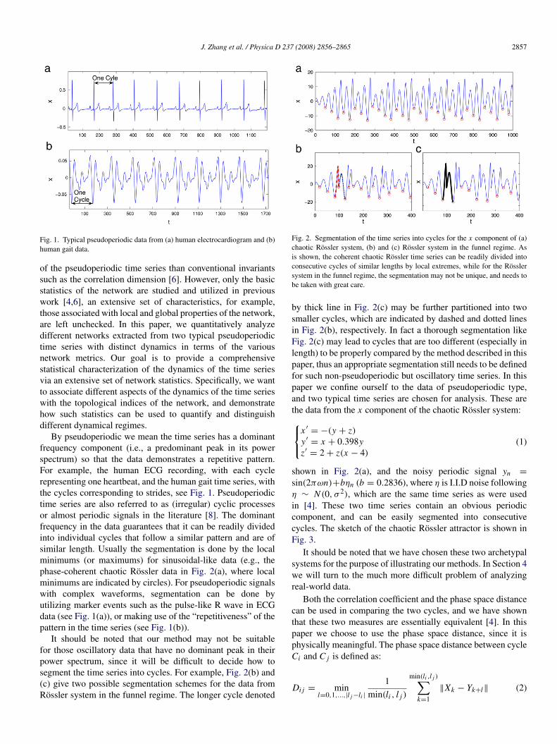
Fig. 1. Typical pseudoperiodic data from (a) human electrocardiogram and (b)human gait data.

of the pseudoperiodic time series than conventional invariantssuch as the correlation dimension [6]. However, only the basicstatistics of the network are studied and utilized in previouswork [4,6], an extensive set of characteristics, for example,those associated with local and global properties of the network,are left unchecked. In this paper, we quantitatively analyzedifferent networks extracted from two typical pseudoperiodictime series with distinct dynamics in terms of the variousnetwork metrics. Our goal is to provide a comprehensivestatistical characterization of the dynamics of the time seriesvia an extensive set of network statistics. Specifically, we wantto associate different aspects of the dynamics of the time serieswith the topological indices of the network, and demonstratehow such statistics can be used to quantify and distinguishdifferent dynamical regimes.

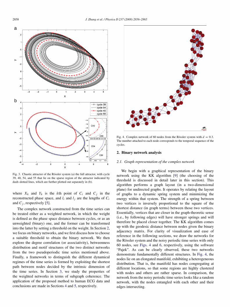
By pseudoperiodic we mean the time series has a dominantfrequency component (i.e., a predominant peak in its powerspectrum) so that the data demonstrates a repetitive pattern.For example, the human ECG recording, with each cyclerepresenting one heartbeat, and the human gait time series, withthe cycles corresponding to strides, see Fig. 1. Pseudoperiodictime series are also referred to as (irregular) cyclic processesor almost periodic signals in the literature [8]. The dominantfrequency in the data guarantees that it can be readily dividedinto individual cycles that follow a similar pattern and are ofsimilar length. Usually the segmentation is done by the localminimums (or maximums) for sinusoidal-like data (e.g., thephase-coherent chaotic Rossler data in Fig. 2(a), where localminimums are indicated by circles). For pseudoperiodic signalswith complex waveforms, segmentation can be done byutilizing marker events such as the pulse-like R wave in ECGdata (see Fig. 1(a)), or making use of the “repetitiveness” of thepattern in the time series (see Fig. 1(b)).

It should be noted that our method may not be suitablefor those oscillatory data that have no dominant peak in theirpower spectrum, since it will be difficult to decide how tosegment the time series into cycles. For example, Fig. 2(b) and(c) give two possible segmentation schemes for the data fromRossler system in the funnel regime. The longer cycle denoted

Fig. 2. Segmentation of the time series into cycles for the x component of (a)chaotic Rossler system, (b) and (c) Rossler system in the funnel regime. Asis shown, the coherent chaotic Rossler time series can be readily divided intoconsecutive cycles of similar lengths by local extremes, while for the Rosslersystem in the funnel regime, the segmentation may not be unique, and needs tobe taken with great care.

by thick line in Fig. 2(c) may be further partitioned into twosmaller cycles, which are indicated by dashed and dotted linesin Fig. 2(b), respectively. In fact a thorough segmentation likeFig. 2(c) may lead to cycles that are too different (especially inlength) to be properly compared by the method described in thispaper, thus an appropriate segmentation still needs to be definedfor such non-pseudoperiodic but oscillatory time series. In thispaper we confine ourself to the data of pseudoperiodic type,and two typical time series are chosen for analysis. These arethe data from the x component of the chaotic Rossler system:!"

#

x # = $(y + z)y# = x + 0.398yz# = 2 + z(x $ 4)

(1)

shown in Fig. 2(a), and the noisy periodic signal yn =sin(2!"n)+b#n (b = 0.2836), where # is I.I.D noise following# % N (0, $ 2), which are the same time series as were usedin [4]. These two time series contain an obvious periodiccomponent, and can be easily segmented into consecutivecycles. The sketch of the chaotic Rossler attractor is shown inFig. 3.

It should be noted that we have chosen these two archetypalsystems for the purpose of illustrating our methods. In Section 4we will turn to the much more difficult problem of analyzingreal-world data.

Both the correlation coefficient and the phase space distancecan be used in comparing the two cycles, and we have shownthat these two measures are essentially equivalent [4]. In thispaper we choose to use the phase space distance, since it isphysically meaningful. The phase space distance between cycleCi and C j is defined as:

Di j = minl=0,1,...,|l j $li |

1min(li , l j )

min(li ,l j )$

k=1

&Xk $ Yk+l& (2)

2858 J. Zhang et al. / Physica D 237 (2008) 2856–2865

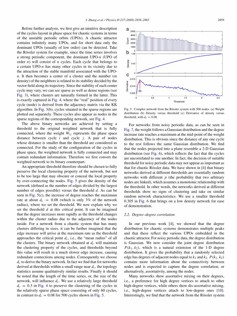
Fig. 3. Chaotic attractor of the Rossler system (a) the full attractor, with cycle39, 40, 54, and 55 that lie on the sparse region of the attractor indicated bydash–dotted lines, which are further plotted out separately in (b).

where Xk and Yk is the kth point of Ci and C j in thereconstructed phase space, and li and l j are the lengths of Ciand C j , respectively [5].

The complex network constructed from the time series canbe treated either as a weighted network, in which the weightis defined as the phase space distance between cycles, or as anunweighted (binary) one, and the former can be transformedinto the latter by setting a threshold on the weight. In Section 2,we focus on binary networks, and we first discuss how to choosea suitable threshold to obtain the binary network. We thenexplore the degree correlation (or associativity), betweennessdistribution and motif structures of the two distinct networksfrom the two pseudoperiodic time series mentioned above.Finally, a framework to distinguish the different dynamicalregimes of the time series is formed by exploiting the shortestpath between nodes decided by the intrinsic dimension ofthe time series. In Section 3, we study the properties ofthe weighted networks in terms of subgraph coherence. Theapplication of the proposed method to human ECG data andconclusions are made in Sections 4 and 5, respectively.

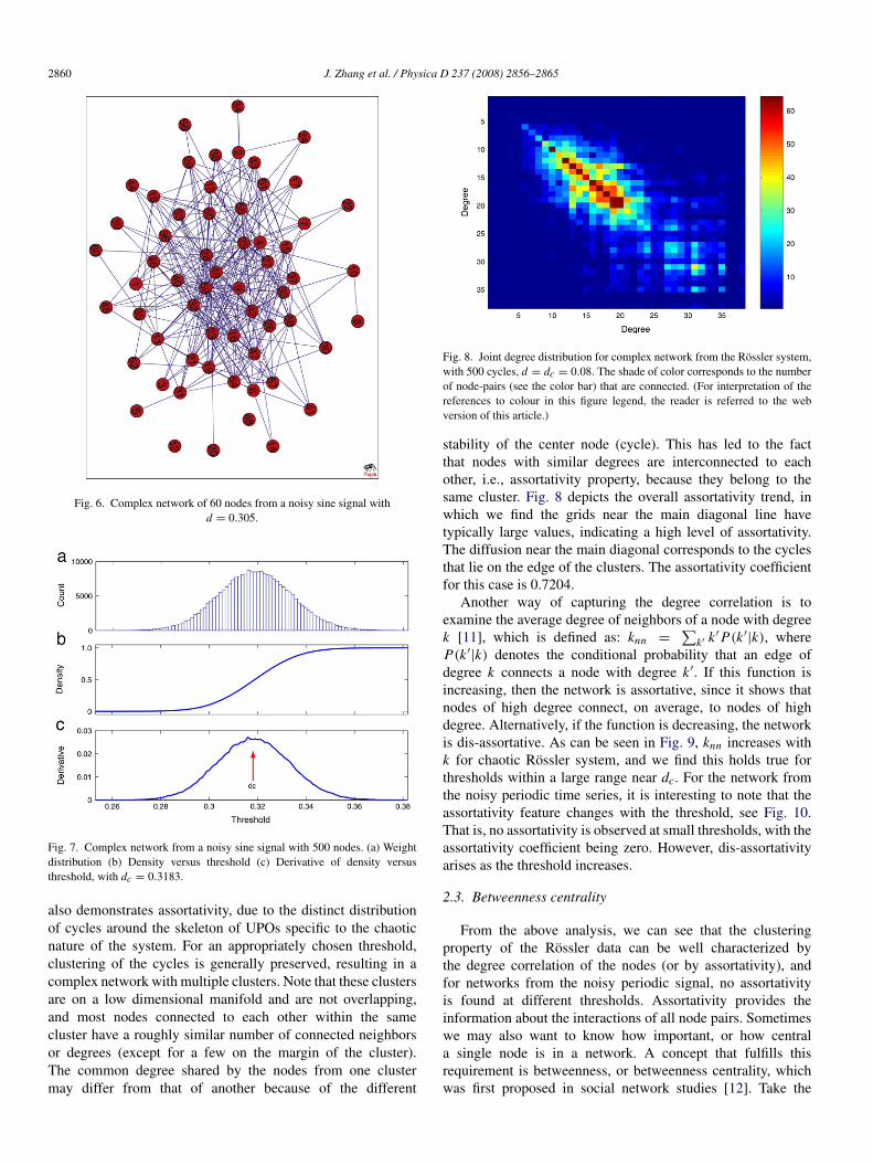
Fig. 4. Complex network of 60 nodes from the Rossler system with d = 0.3.The number attached to each node corresponds to the temporal sequence of thecycles.

2. Binary network analysis

2.1. Graph representation of the complex network

We begin with a graphical representation of the binarynetwork using the KK algorithm [9] (the choosing of thethreshold is discussed in detail later in this section). Thisalgorithm performs a graph layout (in a two-dimensionalplane) for undirected graphs. It operates by relating the layoutof graphs to a dynamic spring system and minimizing theenergy within that system. The strength of a spring betweentwo vertices is inversely proportional to the square of theshortest distance (in graph terms) between those two vertices.Essentially, vertices that are closer in the graph-theoretic sense(i.e., by following edges) will have stronger springs and willtherefore be placed closer together. The KK algorithm comesup with the geodesic distance between nodes given the binaryadjacency matrix. For clarity of visualization and ease ofreference in the following sections, we draw the networks forthe Rossler system and the noisy periodic time series with only60 nodes, see Figs. 4 and 6, respectively, using the software“Pajek”. As can be clearly observed, these two networksdemonstrate fundamentally different structures. In Fig. 4, thenodes lie on an elongated manifold, exhibiting a heterogeneousdistribution. That is, the manifold has nodes congregating atdifferent locations, so that some regions are highly clusteredwith nodes and others are rather sparse. In comparison, thenetwork from the noisy periodic time series looks like a randomnetwork, with the nodes entangled with each other and theiredges intersecting.

J. Zhang et al. / Physica D 237 (2008) 2856–2865 2859

Before further analysis, we first give an intuitive descriptionof the cycles-layout in phase space for chaotic systems in termsof the unstable periodic orbits (UPOs). A chaotic attractorcontains infinitely many UPOs, and for short data only thedominant UPOs (usually of low order) can be detected. Takethe Rossler system for example, since the time series involvesa strong periodic component, the dominant UPO-n (UPO oforder n) will consist of n cycles. Each cycle that belongs toa certain UPO-n has many other cycles in its vicinity due tothe attraction of the stable manifold associated with the UPO-n. It then becomes a center of a cluster and the number (ordensity) of the neighbors is related to its stability decided by thevector field along its trajectory. Since the stability of each centercycle may vary, we can see sparse as well as dense regions (seeFig. 3), where clusters are naturally formed in the latter. Thisis exactly captured in Fig. 4, where the “real” position of everycycle (node) is derived from the adjacency matrix via the KKalgorithm. In Fig. 3(b), cycles situated in the sparse regions areplotted out separately. These cycles also appear as nodes in thesparse regions of the corresponding network, see Fig. 4.

The above binary networks are achieved by setting athreshold to the original weighted network that is fullyconnected, where the weight Wi j represents the phase spacedistance between cycle i and cycle j . A pair of nodeswhose distance is smaller than the threshold are considered asconnected. For the study of the configuration of the cycles inphase space, the weighted network is fully connected and maycontain redundant information. Therefore we first convert theweighted network to its binary counterpart.

An appropriate threshold therefore should be chosen to fullypreserve the local clustering property of the network, but notto be too large that may obscure or conceal the local propertyby over-connecting the nodes. Fig. 5 gives the density of thenetwork (defined as the number of edges divided by the largestnumber of edges possible) versus the threshold d. As can beseen in Fig. 5(c), the increase of degree reaches the maximumrate at about dc = 0.08 (which is only 3% of the networkradius), where we set the threshold. We now explain why weset the threshold d at this critical point. It can be imaginedthat the degree increases more rapidly as the threshold changeswithin the cluster radius due to the adjacency of the nodesinside. For a network from a chaotic system that has manyclusters differing in sizes, it can be further imagined that theedge increase will arrive at the maximum rate as the thresholdapproaches the critical point dc, i.e., the “mean radius” of allthe clusters. The binary network obtained at dc will maintainthe clustering property of the cycles, and thresholds beyondthis value will result in a much slower edge increase, causingredundant connections among nodes. Consequently we choosedc to derive the binary network. In fact we find that for networksderived at thresholds within a small range near dc, the topologystatistics assume qualitatively similar results. Finally it shouldbe noted that the length of the time series, or, the size of thenetwork, will influence dc. We use a relatively large thresholddc = 0.3 in Fig. 4 to preserve the clustering of the cycles inthe relatively sparse phase space consisting of only 60 cycles,in contrast to dc = 0.08 for 500 cycles shown in Fig. 5.

Fig. 5. Complex network from the Rossler system with 500 nodes. (a) Weightdistribution (b) Density versus threshold (c) Derivative of density versusthreshold, with dc = 0.08.

For networks from noisy periodic data, as can be seen inFig. 7, the weight follows a Gaussian distribution and the degreeincrease rate reaches a maximum at the mid-point of the weightdistribution. This is obvious since the distance of any one cycleto the rest follows the same Gaussian distribution. We findthat the nodes projected into a plane resemble a 2-D Gaussiandistribution (see Fig. 6), which reflects the fact that the cyclesare uncorrelated to one another. In fact, the decision of suitablethreshold for noisy periodic data may not appear as important asthat for chaotic Rossler data. We have shown in [4] that binarynetworks derived at different thresholds are essentially randomnetworks with different p (the probability that two arbitrarynodes are linked), which assumes a monotonic relationship withthe threshold. In other words, the networks derived at differentthresholds show no signs of clustering and take on similarrandom network characteristics. We use a smaller threshold0.305 in Fig. 6 that brings on a low density network for easeof demonstration.

2.2. Degree–degree correlation

In our previous work [4], we showed that the degreedistribution for chaotic systems demonstrates multiple peaksand that these reflect the various UPOs embedded in thechaotic attractor. For noisy periodic data, the degree distributionis Gaussian. We now consider the joint degree distributionP(k1, k2), which is a natural extension of the 1-D degreedistribution. It gives the probability that a randomly selectededge has degrees of adjacent nodes equal to k1 and k2. P(k1, k2)

contains more information about the connectivity betweennodes and is expected to capture the degree correlation, oralternatively, assortativity, among the nodes.

Many networks show assortative mixing on their degrees,i.e., a preference for high degree vertices to attach to otherhigh-degree vertices, while others show dis-assortative mixing,i.e., high-degree vertices attach to low-degree ones [10].Interestingly, we find that the network from the Rossler system

2860 J. Zhang et al. / Physica D 237 (2008) 2856–2865

Fig. 6. Complex network of 60 nodes from a noisy sine signal withd = 0.305.

Fig. 7. Complex network from a noisy sine signal with 500 nodes. (a) Weightdistribution (b) Density versus threshold (c) Derivative of density versusthreshold, with dc = 0.3183.

also demonstrates assortativity, due to the distinct distributionof cycles around the skeleton of UPOs specific to the chaoticnature of the system. For an appropriately chosen threshold,clustering of the cycles is generally preserved, resulting in acomplex network with multiple clusters. Note that these clustersare on a low dimensional manifold and are not overlapping,and most nodes connected to each other within the samecluster have a roughly similar number of connected neighborsor degrees (except for a few on the margin of the cluster).The common degree shared by the nodes from one clustermay differ from that of another because of the different

Fig. 8. Joint degree distribution for complex network from the Rossler system,with 500 cycles, d = dc = 0.08. The shade of color corresponds to the numberof node-pairs (see the color bar) that are connected. (For interpretation of thereferences to colour in this figure legend, the reader is referred to the webversion of this article.)

stability of the center node (cycle). This has led to the factthat nodes with similar degrees are interconnected to eachother, i.e., assortativity property, because they belong to thesame cluster. Fig. 8 depicts the overall assortativity trend, inwhich we find the grids near the main diagonal line havetypically large values, indicating a high level of assortativity.The diffusion near the main diagonal corresponds to the cyclesthat lie on the edge of the clusters. The assortativity coefficientfor this case is 0.7204.

Another way of capturing the degree correlation is toexamine the average degree of neighbors of a node with degreek [11], which is defined as: knn = %

k# k# P(k#|k), whereP(k#|k) denotes the conditional probability that an edge ofdegree k connects a node with degree k#. If this function isincreasing, then the network is assortative, since it shows thatnodes of high degree connect, on average, to nodes of highdegree. Alternatively, if the function is decreasing, the networkis dis-assortative. As can be seen in Fig. 9, knn increases withk for chaotic Rossler system, and we find this holds true forthresholds within a large range near dc. For the network fromthe noisy periodic time series, it is interesting to note that theassortativity feature changes with the threshold, see Fig. 10.That is, no assortativity is observed at small thresholds, with theassortativity coefficient being zero. However, dis-assortativityarises as the threshold increases.

2.3. Betweenness centrality

From the above analysis, we can see that the clusteringproperty of the Rossler data can be well characterized bythe degree correlation of the nodes (or by assortativity), andfor networks from the noisy periodic signal, no assortativityis found at different thresholds. Assortativity provides theinformation about the interactions of all node pairs. Sometimeswe may also want to know how important, or how centrala single node is in a network. A concept that fulfills thisrequirement is betweenness, or betweenness centrality, whichwas first proposed in social network studies [12]. Take the

J. Zhang et al. / Physica D 237 (2008) 2856–2865 2861

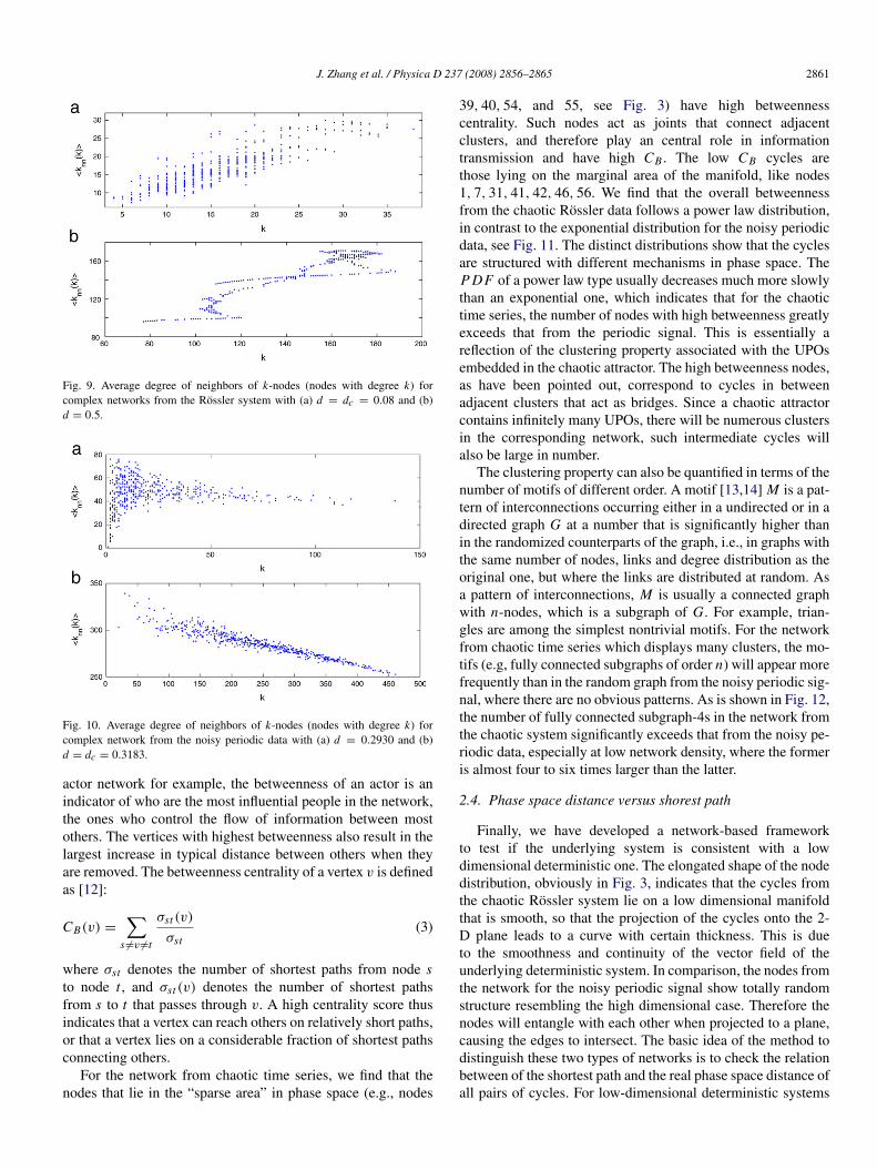
Fig. 9. Average degree of neighbors of k-nodes (nodes with degree k) forcomplex networks from the Rossler system with (a) d = dc = 0.08 and (b)d = 0.5.

Fig. 10. Average degree of neighbors of k-nodes (nodes with degree k) forcomplex network from the noisy periodic data with (a) d = 0.2930 and (b)d = dc = 0.3183.

actor network for example, the betweenness of an actor is anindicator of who are the most influential people in the network,the ones who control the flow of information between mostothers. The vertices with highest betweenness also result in thelargest increase in typical distance between others when theyare removed. The betweenness centrality of a vertex v is definedas [12]:

CB(v) =$

s '=v '=t

$st (v)

$st(3)

where $st denotes the number of shortest paths from node sto node t , and $st (v) denotes the number of shortest pathsfrom s to t that passes through v. A high centrality score thusindicates that a vertex can reach others on relatively short paths,or that a vertex lies on a considerable fraction of shortest pathsconnecting others.

For the network from chaotic time series, we find that thenodes that lie in the “sparse area” in phase space (e.g., nodes

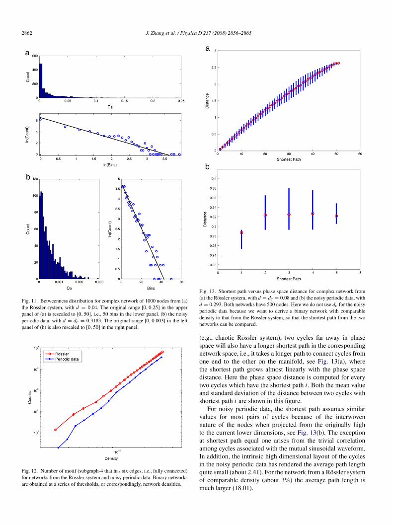
39, 40, 54, and 55, see Fig. 3) have high betweennesscentrality. Such nodes act as joints that connect adjacentclusters, and therefore play an central role in informationtransmission and have high CB . The low CB cycles arethose lying on the marginal area of the manifold, like nodes1, 7, 31, 41, 42, 46, 56. We find that the overall betweennessfrom the chaotic Rossler data follows a power law distribution,in contrast to the exponential distribution for the noisy periodicdata, see Fig. 11. The distinct distributions show that the cyclesare structured with different mechanisms in phase space. TheP DF of a power law type usually decreases much more slowlythan an exponential one, which indicates that for the chaotictime series, the number of nodes with high betweenness greatlyexceeds that from the periodic signal. This is essentially areflection of the clustering property associated with the UPOsembedded in the chaotic attractor. The high betweenness nodes,as have been pointed out, correspond to cycles in betweenadjacent clusters that act as bridges. Since a chaotic attractorcontains infinitely many UPOs, there will be numerous clustersin the corresponding network, such intermediate cycles willalso be large in number.

The clustering property can also be quantified in terms of thenumber of motifs of different order. A motif [13,14] M is a pat-tern of interconnections occurring either in a undirected or in adirected graph G at a number that is significantly higher thanin the randomized counterparts of the graph, i.e., in graphs withthe same number of nodes, links and degree distribution as theoriginal one, but where the links are distributed at random. Asa pattern of interconnections, M is usually a connected graphwith n-nodes, which is a subgraph of G. For example, trian-gles are among the simplest nontrivial motifs. For the networkfrom chaotic time series which displays many clusters, the mo-tifs (e.g, fully connected subgraphs of order n) will appear morefrequently than in the random graph from the noisy periodic sig-nal, where there are no obvious patterns. As is shown in Fig. 12,the number of fully connected subgraph-4s in the network fromthe chaotic system significantly exceeds that from the noisy pe-riodic data, especially at low network density, where the formeris almost four to six times larger than the latter.

2.4. Phase space distance versus shorest path

Finally, we have developed a network-based frameworkto test if the underlying system is consistent with a lowdimensional deterministic one. The elongated shape of the nodedistribution, obviously in Fig. 3, indicates that the cycles fromthe chaotic Rossler system lie on a low dimensional manifoldthat is smooth, so that the projection of the cycles onto the 2-D plane leads to a curve with certain thickness. This is dueto the smoothness and continuity of the vector field of theunderlying deterministic system. In comparison, the nodes fromthe network for the noisy periodic signal show totally randomstructure resembling the high dimensional case. Therefore thenodes will entangle with each other when projected to a plane,causing the edges to intersect. The basic idea of the method todistinguish these two types of networks is to check the relationbetween of the shortest path and the real phase space distance ofall pairs of cycles. For low-dimensional deterministic systems

2862 J. Zhang et al. / Physica D 237 (2008) 2856–2865

Fig. 11. Betweenness distribution for complex network of 1000 nodes from (a)the Rossler system, with d = 0.04. The original range [0, 0.25] in the upperpanel of (a) is rescaled to [0, 50], i.e., 50 bins in the lower panel. (b) the noisyperiodic data, with d = dc = 0.3183. The original range [0, 0.003] in the leftpanel of (b) is also rescaled to [0, 50] in the right panel.

Fig. 12. Number of motif (subgraph-4 that has six edges, i.e., fully connected)for networks from the Rossler system and noisy periodic data. Binary networksare obtained at a series of thresholds, or correspondingly, network densities.

Fig. 13. Shortest path versus phase space distance for complex network from(a) the Rossler system, with d = dc = 0.08 and (b) the noisy periodic data, withd = 0.293. Both networks have 500 nodes. Here we do not use dc for the noisyperiodic data because we want to derive a binary network with comparabledensity to that from the Rossler system, so that the shortest path from the twonetworks can be compared.

(e.g., chaotic Rossler system), two cycles far away in phasespace will also have a longer shortest path in the correspondingnetwork space, i.e., it takes a longer path to connect cycles fromone end to the other on the manifold, see Fig. 13(a), wherethe shortest path grows almost linearly with the phase spacedistance. Here the phase space distance is computed for everytwo cycles which have the shortest path i . Both the mean valueand standard deviation of the distance between two cycles withshortest path i are shown in this figure.

For noisy periodic data, the shortest path assumes similarvalues for most pairs of cycles because of the interwovennature of the nodes when projected from the originally highto the current lower dimensions, see Fig. 13(b). The exceptionat shortest path equal one arises from the trivial correlationamong cycles associated with the mutual sinusoidal waveform.In addition, the intrinsic high dimensional layout of the cyclesin the noisy periodic data has rendered the average path lengthquite small (about 2.41). For the network from a Rossler systemof comparable density (about 3%) the average path length ismuch larger (18.01).

J. Zhang et al. / Physica D 237 (2008) 2856–2865 2863

3. Weighted network analysis

Up to now we have focused only on the binary networkderived with an appropriate threshold from the originalweighted network. In this section, we treat the network as afully connected one with the weight between two nodes beingthe phase space distance between corresponding cycles. Inparticular, we consider the subgraph intensity and coherence ofthe weighted network.

Onnela et al. have recently proposed a systematic way toextend motifs to a weighted graph GW = (N , L , W ) [15].A motif M is defined as a set of the topological equivalentsubgraphs of GW . The intensity I (g) and the coherence Q(g)

of a given subgraph g = (Ng, Lg, Wg) with n nodes and l linksare defined as:

I (g) = W1

|lg | , Q(g) = I (g) · |lg|/W (4)

respectively, where W = &(i, j)(lg

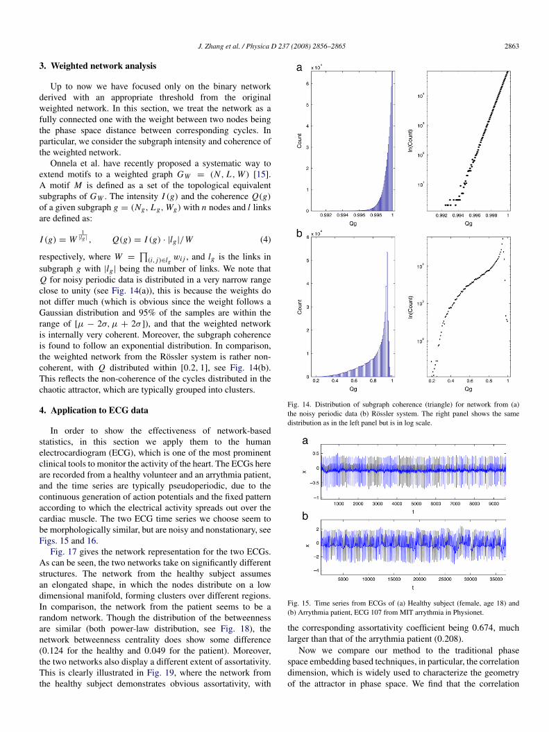
wi j , and lg is the links insubgraph g with |lg| being the number of links. We note thatQ for noisy periodic data is distributed in a very narrow rangeclose to unity (see Fig. 14(a)), this is because the weights donot differ much (which is obvious since the weight follows aGaussian distribution and 95% of the samples are within therange of [µ $ 2$, µ + 2$ ]), and that the weighted networkis internally very coherent. Moreover, the subgraph coherenceis found to follow an exponential distribution. In comparison,the weighted network from the Rossler system is rather non-coherent, with Q distributed within [0.2, 1], see Fig. 14(b).This reflects the non-coherence of the cycles distributed in thechaotic attractor, which are typically grouped into clusters.

4. Application to ECG data

In order to show the effectiveness of network-basedstatistics, in this section we apply them to the humanelectrocardiogram (ECG), which is one of the most prominentclinical tools to monitor the activity of the heart. The ECGs hereare recorded from a healthy volunteer and an arrythmia patient,and the time series are typically pseudoperiodic, due to thecontinuous generation of action potentials and the fixed patternaccording to which the electrical activity spreads out over thecardiac muscle. The two ECG time series we choose seem tobe morphologically similar, but are noisy and nonstationary, seeFigs. 15 and 16.

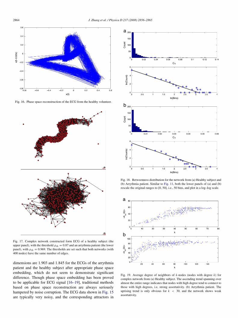
Fig. 17 gives the network representation for the two ECGs.As can be seen, the two networks take on significantly differentstructures. The network from the healthy subject assumesan elongated shape, in which the nodes distribute on a lowdimensional manifold, forming clusters over different regions.In comparison, the network from the patient seems to be arandom network. Though the distribution of the betweennessare similar (both power-law distribution, see Fig. 18), thenetwork betweenness centrality does show some difference(0.124 for the healthy and 0.049 for the patient). Moreover,the two networks also display a different extent of assortativity.This is clearly illustrated in Fig. 19, where the network fromthe healthy subject demonstrates obvious assortativity, with

Fig. 14. Distribution of subgraph coherence (triangle) for network from (a)the noisy periodic data (b) Rossler system. The right panel shows the samedistribution as in the left panel but is in log scale.

Fig. 15. Time series from ECGs of (a) Healthy subject (female, age 18) and(b) Arrythmia patient, ECG 107 from MIT arrythmia in Physionet.

the corresponding assortativity coefficient being 0.674, muchlarger than that of the arrythmia patient (0.208).

Now we compare our method to the traditional phasespace embedding based techniques, in particular, the correlationdimension, which is widely used to characterize the geometryof the attractor in phase space. We find that the correlation

2864 J. Zhang et al. / Physica D 237 (2008) 2856–2865

Fig. 16. Phase space reconstruction of the ECG from the healthy volunteer.

Fig. 17. Complex network constructed form ECG of a healthy subject (theupper panel), with the threshold %th = 0.87 and an arrythmia patient (the lowerpanel), with %th = 0.969. The thresholds are set such that both networks (with400 nodes) have the same number of edges.

dimensions are 1.903 and 1.845 for the ECGs of the arrythmiapatient and the healthy subject after appropriate phase spaceembedding, which do not seem to demonstrate significantdifference. Though phase space embedding has been provedto be applicable for ECG signal [16–19], traditional methodsbased on phase space reconstruction are always seriouslyhampered by noise corruption. The ECG data shown in Fig. 15are typically very noisy, and the corresponding attractors in

Fig. 18. Betweenness distribution for the network from (a) Healthy subject and(b) Arrythmia patient. Similar to Fig. 11, both the lower panels of (a) and (b)rescale the original ranges to [0, 50], i.e., 50 bins, and plot in a log–log scale.

Fig. 19. Average degree of neighbors of k-nodes (nodes with degree k) forcomplex network from (a) Healthy subject. The ascending trend spanning overalmost the entire range indicates that nodes with high degree tend to connect tothose with high degrees, i.e, strong assortativity. (b) Arrythmia patient. Theuprising trend is only obvious for k < 30, and the network shows weakassortativity.

J. Zhang et al. / Physica D 237 (2008) 2856–2865 2865

phase space seem to be dominated by the noise component thatsmears the fine structure of the ECG data (see Fig. 16). Fromthis comparison we can see that the network representationof the ECG on the cycle scale helps to reveal the essentialdifference between the data structures of the healthy subjectand the patient, which tends to be masked by noise and isinvisible to conventional methods that calculate on the pointscale. Application of the proposed network transformation tolarger and different datasets, however, is needed to test itsperformance more objectively.

5. Discussion

The pseudoperiodic signals are naturally simplified bytreating each cycle, rather than each sampling point, as the basicunit. Another technique that has similar effect is the Poincaresection method. The Poincare section is the intersection offlow data in the state space with a certain lower dimensionalsubspace, or hyperplane, which is transversal to the flow of thesystem. The highly sampled data representing the continuoustime of a dynamical system are reduced to a new vector series,which each vector representing the corresponding cycle inthe pseudoperiodic time series. Usually, the placement of thePoincare surface is of high relevance for the usefulness of theresult. Our construction of the complex network relies on thesegmentation of the pseudoperiodic time series, and this isequivalent to choosing the location of the Poincare section.

Both methods depend on an appropriate segmentation ofthe time series, if one defines a Poincare surface as the zerocrossings of the temporal derivative of the signal, then thisis synonymous with collecting all maxima or all minima,which is the procedure we have used to divide the time seriesinto cycles. Nevertheless, these two methods reflect differentsources of information from the underlying system and possessdifferent level of robustness. Discrete points on the Poincaresection only specify the dynamics of the map at that sectionand the information regarding the trajectories that connect thePoincare section points are inevitably lost, and such dynamicsare liable to change with the section and are vulnerable tonoise. Comparatively, we utilize all the points associated witha cycle and characterize the correlation among the cycles. Thusnot only the full information of the trajectory is kept, but themethod becomes more robust to noise. Although our methodalso depends on the segmentation scheme, the correlationstructures of the networks derived from different segmentationsare essentially very similar.

The connection of our method to the Poincare sectionreminds one of symbolic dynamics analysis, by which theRossler system can also be analyzed. It embeds as a one humpmap that gives rise to a full-shift on two symbols. Thoughit would be interesting to associate our framework with thetraditional symbolic dynamics, this is not the focus of thispaper. Indeed we note that a large variety of real-world signalsare too noisy and nonstationary to be effectively exploredand characterized via the traditional methods as have beenpreviously described. The motivation of this paper thereforeis to reliably characterize the correlation structure among the

cycles first, before attempting to understand the mathematicalorigin of the dynamics.

In summary, we have explored an extensive set oftopological statistics for the networks constructed from twopseudoperiodic time series with distinct dynamics, i.e., thedeterministic chaotic Rossler time series and the stochasticnoisy periodic data. The essential features of these twokinds of time series are that the cycles from the formerlie on a low dimensional manifold, with their correlationmanifested in the strong local clustering, while cycles fromthe latter are randomly correlated and cannot be effectivelyrepresented in a low dimensional space. We find that thejoint degree distribution appears to fundamentally characterizethe clustering property of the cycles induced by the UPOsintrinsic to the chaotic attractor. The extent of assortativity,as a single-value quantification of joint degree distribution,appears to be efficient in distinguishing different sorts ofnetworks derived from various time series. In addition, thebetweenness centrality and the motif also achieve differentextent of success in discriminating different dynamical regimesin the pseudoperiodic time series. We demonstrate that thetopological statistics discussed in this paper combine to providean all-around characterization on how cycles are structured inphase space, and furthermore a comprehensive quantification ofthe dynamics of the pseudoperiodic time series. Application tohuman electrocardiograms shows that this alternative approachis effective in differentiating healthy subjects from arrythmiapatients.

Acknowledgement

This research is funded by the Hong Kong PolytechnicUniversity Postdoctoral Fellowships Scheme 2007-08 (G-YX0N).

References

[1] R. Albert, A.-L. Barabasi, Rev. Modern Phys. 74 (2002) 47–97.[2] M.E.J. Newman, SIAM Rev. 45 (2) (2003) 167–256.[3] S. Boccaletti, V. Latora, Y. Moreno, M. Chavez, D.-U. Hwang, Phys. Rep.

424 (2006) 175–308.[4] J. Zhang, M. Small, Phys. Rev. Lett. 96 (2006) 238701.[5] J. Zhang, X. Luo, M. Small, Phys. Rev. E 73 (2006) 016216.[6] J. Zhang, X. Luo, N. Tomomichi, J. Sun, M. Small, Phys. Rev. E 73 (2006)

016218.[7] M. Small, D.J. Yu, R.G. Harrison, Phys. Rev. Lett. 87 (2001) 188101.[8] P.P. Kanjilal, J. Bhattacharya, G. Saha, Phys. Rev. E 59 (1999) 4013.[9] T. Kamada, S. Kawai, Inform. Process. Lett. 31 (1) (1989) 7–15.

[10] M.E.J. Newman, Phys. Rev. Lett. 89 (2002) 208701.[11] R. Pastor-Satorras, A. Vazquez, A. Vespignani, Phys. Rev. Lett. 87 (2001)

258701.[12] L.C. Freeman, Sociometry 40 (1977) 35–41.[13] S. Shen-Orr, R. Milo, S. Mangan, U. Alon, Nature Gen. 31 (2002) 64–68.[14] R. Milo, S. Shen-Orr, S. Itzkovitz, N. Kashan, D. Chklovskii, U. Alon,

Science 298 (2002) 824.[15] O. Jukka-Pekka, S. Jari, K. Janos, K. Kimmo, Phys. Rev. E 71 (2005)

065103(R).[16] M. Richter, T. Schreiber, Phys. Rev. E 58 (1998) 6392–6398.[17] M. Small, D.J. Yu, R.G. Harrison, C. Robertson, G. Clegg, M. Holzer,

F. Sterz, Chaos 10 (2000) 268–277.[18] M. Small, D.J. Yu, R. Clayton, T. Eftestol, K. Sunde, P.A. Steen,

R.G. Harrison, Int. J. Bifur. Chaos 11 (2001) 2531–2548.[19] M. Small, D.J. Yu, J. Simonotto, R.G. Harrison, N. Grubb, K.A.A. Fox,

Chaos Solitons Fractals 13 (2002) 1755–1762.