Characterizing Global Investors' Risk Appetite for Emerging Market Debt During Financial Crises
44
WP/03/251 Characterizing Global Investors’ Risk Appetite for Emerging Market Debt During Financial Crises Mardi Dungey, Renée Fry, Brenda González-Hermosillo, and Vance Martin
-
Upload
independent -
Category
Documents
-
view
3 -
download
0
Transcript of Characterizing Global Investors' Risk Appetite for Emerging Market Debt During Financial Crises

WP/03/251
Characterizing Global Investors’ Risk Appetite for Emerging Market Debt
During Financial Crises
Mardi Dungey, Renée Fry, Brenda González-Hermosillo,
and Vance Martin

© 2003 International Monetary Fund WP/03/251
IMF Working Paper
IMF Institute
Characterizing Global Investors’ Risk Appetite for Emerging Market Debt During Financial Crises
Prepared by Mardi Dungey, Renée Fry, Brenda González-Hermosillo, and Vance Martin1
Authorized for distribution by Sunil Sharma
December 2003
Abstract
This Working Paper should not be reported as representing views of the IMF. The views expressed in this Working Paper are those of the author(s) and do not necessarily represent those of the IMF or IMF policy. Working Papers describe research in progress by the author(s) and are published to elicit comments and to further debate.
The effects of unanticipated movements in global risk on nine emerging bond markets are investigated. The components of global risk are volatility, credit, and liquidity risks. Country and contagion risks are also studied individually. A historical decomposition of bond spreads is used to identify the relative contributions of risk during 1998–99. The empirical results show that the Russian/LTCM crises were characterized by increases in global credit risk, while the relative size of global risk factors was mixed for the Brazilian crisis, with no component dominating. Country risk is found to be important for all countries, while there is little evidence of contagion risk. JEL Classification Numbers: C33, E44, F34
Keywords: Risk Aversion, Bond Markets, Financial Crises, SVAR
Authors’ E-Mail Addresses: [email protected], [email protected],
[email protected], [email protected] 1 Mardi Dungey and Renée Fry are from the Australian National University, Brenda González-Hermosillo is from the IMF, and Vance Martin is from the University of Melbourne. Dungey and Martin acknowledge funding from ARC Large Grant A00001350. The authors are grateful to IMF International Capital Markets seminar participants, the UNSW CAER Summer Macroeconomics Workshop, University of Warwick Summer Workshop 2003, ANU seminar participants, Prasanna Gai, Marcus Miller, Adrian Pagan, Olwen Renowden, and David Vines for helpful comments.
- 2 -
Contents Page
I. Introduction ............................................................................................................................4
II. An Empirical Model of Risk Premia.....................................................................................6 A. SVAR Specification..................................................................................................7 B. Long-Run Identifying Restrictions............................................................................9 C. Estimation................................................................................................................12 D. Historical Decomposition Methodology.................................................................12
III. Empirical Results ...............................................................................................................13 A. Benchmark Prices Based on Precrisis Information.................................................19 B. Risk Factors.............................................................................................................20
IV. Conclusions and Suggestions for Future Research............................................................23 Appendices I. Data Definitions and Sources .............................................................................................26 II. Descriptive Statistics ..........................................................................................................28 III. Parameter Estimates...........................................................................................................30
References................................................................................................................................31 Text Tables 1. Mean and Standard Deviation of Benchmark Prices Over the Crisis Period Based on Precrisis Information (percentage points) ............................................................19 2. Mean Decomposition of Spreads During Each Crisis .........................................................22 Appendix Tables A2.1. Descriptive Statistics of the Bond Spreads, February 12, 1998 to May 17, 1999 .........28 A2.2. Descriptive Statistics of the Log of the J.P. Morgan Volatility and Liquidity Risk Indices, and the Credit Variable, February 12, 1998 to May 17, 1999..........................28 A2.3. Descriptive Statistics of Changes in the Bond Spreads, February 12, 1998 to May 17, 1999 .................................................................................................................29 A2.4. Descriptive Statistics of the Change in the Log of the J.P. Morgan Volatility and Liquidity Risk Indices, and the Percentage Change in the Credit Variable, February 12, 1998 to May 17, 1999...............................................................................29 A3.1. Long-Run Parameter Estimates of H in (13) ................................................................30 Figures 1. Bond Spreads (percent), February 1998 – May 1999 ........................................................16 2. Bond Spreads (Percentage Change), February 1998 – May 1999 .....................................17 3. Risk Variables, February 1998 – May 1999 ......................................................................18 4. Decomposition of Bond Spreads – Argentina ...................................................................35

- 3 -
5. Decomposition of Bond Spreads – Brazil..........................................................................36 6. Decomposition of Bond Spreads – Mexico .......................................................................37 7. Decomposition of Bond Spreads – Indonesia....................................................................38 8. Decomposition of Bond Spreads - Republic of Korea......................................................39 9. Decomposition of Bond Spreads – Thailand .....................................................................40 10. Decomposition of Bond Spreads – Bulgaria......................................................................41 11. Decomposition of Bond Spreads – Republic of Poland.....................................................42 12. Decomposition of Bond Spreads – Russia.........................................................................43

- 4 -
I. INTRODUCTION A key characteristic of recent financial crises is that they tend to cluster. Anecdotal evidence suggests that periods of distress across global financial markets coincide with reduced international appetite for risk. Recent IMF Global Financial Stability reports suggest that changing risk preferences may either widen or narrow emerging market bond spreads (International Monetary Fund, 2002, 2003a, 2003b). In this paper we consider the contribution of changing risk preferences to the rapid widening of emerging market bond spreads during February 1998–May 1999. This period encompasses the Russian, LTCM, and Brazilian crises. The role of changes in investors’ risk appetite in transmitting financial crises has been investigated in Kumar and Persaud (2001) and Missina (2003).2
Risk appetite and the state of investors’ balance sheets in developed markets are important contributors to global financial conditions (Bank of England, 2002, and Mody and Taylor, 2002). In particular, international markets are affected by investors’ rebalancing their portfolios following a shock (Kodres and Pritsker, 2002, and Schinasi and Smith,1999); common lender effects (Van Rijckeghem and Weder, 2000); and heightened risk aversion (J.P. Morgan, 1999, International Monetary Fund, 2002, 2003a, 2003b). Liquidity considerations may also play a role, where liquid assets may be offloaded despite their relatively low default risk (Greenspan, 1999).
The presence of so-called “crossover investors,” who view high-yield investments in advanced financial markets and emerging market debt as equivalently risky assets, may explain some clustering of financial crises in seemingly unrelated countries (International Monetary Fund, 2002). This aspect of financial markets has not received much attention in the literature, owing to the difficulty in identifying such effects.
Risk aversion is difficult to measure. The spreads of sovereign bonds of emerging markets capture the risk premia attached to particular countries, thus reflecting its default risk but also the degree of unwillingness to buy that country’s debt. The latter may be unrelated to the actual default risk, but instead reflect factors such as the financial position of investors, liquidity risk in financial markets, or investors’ risk appetite at that time. Despite these limitations, one empirical approach to measuring changes in global risk patterns is suggested by J.P. Morgan Chase Bank (2002) using risk indices.3 2 Other literature investigate alternative channels of transmission of crises. For example: contagion in Masson (1999), Calvo and Mendoza (2000), and Pericoli and Sbracia (2003) for a summary; market fundamentals in Eichengreen, Rose and Syplosz (1996); trade linkages in Glick and Rose (1999), and Forbes (2001); financial linkages in Van Rijckeghem and Weder (2003); and common external shocks such as higher U.S. interest rates in Gertler and Lown (2000), and Forbes and Rigobon (2002).
3 Hereafter denoted as J.P. Morgan in the text.

- 5 -
The J.P. Morgan indices attempt to identify various components of global risk including liquidity risk, credit risk, and volatility risk (LCVI). Liquidity risk is measured by the premium factored into the spread between on-the-run and off-the-run government bonds, which otherwise have the same credit risk; credit risk is given by the spread between long-term investment grade corporate bonds and a risk-free rate; while volatility risk is based on the implied volatiltiy of options markets. Associated with these sub-indices is an index of global risk aversion which combines the three sub-components. This index is particularly interesting as it was developed to circumvent the problems associated with measuring risk within a single asset class, and is often used as an approximation for risk aversion in global financial markets (International Monetary Fund, 2002, 2003a).
A second approach to measuring changes in risk patterns is theoretically based, where risk is identified through a dynamic optimization problem that predicts that the risk premia is a function of the quantity of risk and the price of risk. The quantity of risk is represented by the covariance between a set of factor shocks and the risk premia of the asset (Campbell, 1996; Cochrane, 2001; Cochrane and Piazzesi, 2001). In models of the risk premium on equities, the covariance is between the risk premia and the excess return on all invested wealth in the capital asset pricing model (Sharpe, 1964; Lintner, 1965), whereas in the consumption-based capital asset pricing model (CCAPM) the pertinent covariance is between the risk premia and consumption (Breeden, 1979; Grossman and Shiller, 1981). For power utility preferences the price of risk equals the relative risk aversion parameter in the CCAPM.
The approach adopted here is to exploit both methods for identifying risk. This is achieved by formulating a multifactor asset-pricing model for the risk premia of emerging bond markets where the factor shocks are the risk components of the J.P. Morgan indices. The model is based on a structural vector autoregression (SVAR) where identification of structural shocks is through the imposition of restrictions on the long-run risk characteristics of the variables. The model is applied to daily bond spreads of nine emerging markets during 1998–99. Three crises are covered: the Russian default on August 17, 1998, the near-collapse of the highly leveraged U.S. hedge fund, Long-Term Capital Management (LTCM), publicly announced on September 23, 1998, and the speculative attack on the Brazilian real on January 13, 1999, which followed several months of increased pressure on Brazilian markets. In response to the Russian and LTCM crises, bond spreads jumped globally, even for otherwise seemingly unconnected countries (Kumar and Persaud, 2001; Committee on the Global Financial System, 1999; J.P. Morgan, 1999; and Bank of England, 2002). The Russian and LTCM crises were reinforcing, and it seems likely that global risk conditions influenced other financial markets, including the equity markets, and exacerbated the conditions facing Brazil (Dungey, Fry, González-Hermosillo, and Martin, 2002, 2003).4 4 For an overview of the background of events surrounding the Russian and LTCM crises, see Dungey, Fry, González-Hermosillo, and Martin, 2002a, 2002b; the Committee on the Global Financial System, 1999; and Jorion, 2000. For an overview of the Brazilian crisis, see Goldfajn and Valdez, 1997.

- 6 -
The impact of shocks due to risk factors during these episodes is disentangled using a historical decomposition of the SVAR. This decomposition provides a convenient breakdown of the risk premia into contributions from global shocks in risk (volatility, credit, and liquidity), country risk stemming from shocks occurring within a country, and contagion risk, which arises from the transmission of shocks between emerging markets and across regions. Each crisis is then distinguished by its risk characteristics. In addition, benchmark prices for each emerging market are calculated as conditional forecasts formed in June 1998. This date is arbitrarily chosen to capture a period of relative stability in global financial markets prior to the onset of the Russian crisis. These prices are used to provide an objective measure of the impact of the subsequent crises in terms of yield spreads over the benchmark price.
The empirical results show that increases in the risk premium of emerging markets
during the Russian/LTCM crises is primarily due to increases in credit risk and country risk. Russian sovereign bonds experience the largest increase in credit risk during the crisis—where the additional risk premium for credit is between 15 and 20 percent. During the Brazilian crisis, credit risk is not as clearly dominant. The contributions of the various risk components vary both across and within regions during the Brazilian crisis. In general, country risk is found to be important in all countries, especially in the case of Brazil, Indonesia, the Republic of Poland and Russia. The results show little evidence of contagion arising from unanticipated shocks across national borders. The remainder of this paper is organized as follows. The modelling framework is developed in Section II for identifying the contributions of alternative types of risk in explaining changes in bond spreads during financial crises. The model is applied in Section III to decompose bond spreads during 1998–99, with special attention given to understanding changes in risk patterns during the Russian/LTCM and Brazilian crises. Concluding comments and some suggestions for future research are contained in Section IV.
II. AN EMPIRICAL MODEL OF RISK PREMIA
In this section, a SVAR model is developed for decomposing movements in the bond spreads of nine emerging markets. The emerging markets considered in the empirical analysis are Argentina, Brazil and Mexico from Latin America; Indonesia, the Republic of Korea and Thailand from Asia; and Bulgaria, the Republic of Poland and Russia from Eastern Europe. In decomposing bond spreads a number of factors are considered, including benchmark prices which refer to yields that would occur if a crisis had not occurred, various components of changes in global risk, country risk, and the contributions arising from shocks in bond spreads of other emerging markets. The global risk factors investigated consist of three components: volatility, liquidity and credit. These factors represent the effects of contagion from the impact of common shocks originating in developed financial markets. The inclusion of the transmission of shocks across national bond markets allows for potential contagious channels investigated by Dungey, Fry, González-Hermosillo and Martin (2002a,b,c). Thus, two potential channels of contagion are examined: the first represents the effect of common financial shocks on emerging markets arising in developed financial

- 7 -
markets, and the second corresponding to the effects of unanticipated shocks across national bond markets.
A. SVAR Specification
The total number of variables investigated in the SVAR is N=12, consisting of the
risk premia of the nine countries investigated and the three variables that measure the different components of changes in global risk. Let the full set of variables be summarized by
.,,, ,titttt SPREADSLIQUIDITYCREDITVOLATILITYZ = (3)
A convenient framework in which to model the dynamics of the variables over time is a vector autoregression (VAR)
( ) ,...2
21 ttp
p eZLLLI +=∆Φ−−Φ−Φ− α (4) where k
t t kL Z Z −= is the lag operator, ( )LI −=∆ is the first difference operator, kΦ are (12×12) matrices of autoregressive parameters, α is a (12×1) vector of intercept parameters to capture the levels of the variables, and te is a 12-variate multivariate normal random error
with zero mean [ ] 0tE e = , a contemporaneous covariance matrix t tE e e ′ = Ω , and are non-
autocorrelated 0, 0t t sE e e s− ′ = ∀ ≠
. The assumption of a constant residual variance-
covariance matrix could be relaxed by specifying a richer set of dynamics for the second moments.5 To identify the sources of shocks underlying the movements in the variables in the VAR, the vector moving average (VMA) representation of the VAR is derived by inverting the matrix polynomial 2
1 2I- ,ppL L LΦ −Φ − −Φ… in (4)
( ) ( )
( ) ,...
,...2
21
1221
tq
qt
tp
pt
eLLLIZ
eLLLIZ
Θ−−Θ−Θ−+=∆
+Φ−−Φ−Φ−=∆−
β
α (5)
5 One way to proceed would be to use a multivariate GARCH model following the work of Bekaert, Harvey, and Ng (2003), for example. An alternative approach would be to adopt a factor GARCH model along the lines of Dungey, Fry, González-Hermosillo, and Martin (2002a).

- 8 -
where kΘ are (12×12) matrices of moving average parameters which are functions of the
autoregressive parameters of the VAR, and ( ) 1
1 2I- pβ α−
= Φ −Φ − −Φ… is a (12×1) vector
of intercept parameters.6 The VMA has an infinite lag structure, although as tZ∆ is covariance stationary, the moving average parameter matrices eventually die out for longer lags. The main aim of the empirical modeling is to isolate the separate effects of shocks in volatility, liquidity and credit in developed markets on the bond spreads in emerging markets. To achieve this, it is necessary to transform the VAR as the shocks te are contemporaneously correlated. Letting tv represent a set of independent structural shocks, the pertinent transformation is given by t te Gv= (6) where G represents a matrix of unknown “structural” parameters, and tv contains the set of
independent shocks which have the properties [ ] 0,tE v = , ,t tE v v I ′ = and
, 0 0.t t sE v v s− ′ = ∀ ≠
From the properties of et in (4), 'GG=Ω . Substituting (6) into (5)
shows that by redefining the moving average structure for the set of bond spreads as well as the movements in the risk variables, the dynamics of the model can be expressed in terms of the separate shocks underlying all processes
( ) ,...2210 t
qqt GvLLLZ Θ−−Θ−Θ−Θ+=∆ β (7)
where 0 IΘ = . From (7), the effect of a structural shock at time t, on the changes in the variables at time t+s is immediately given by
' .t ss
t
Z Gv
+∂∆= Θ
∂ (8)
Alternatively, the effect of a shock at time t on the level of the variables at time t+s, is the cumulative sum of the shocks over the period
6 The matrix polynomial inversion used to generate the vector moving average representation is usually computed numerically; see Hamilton (1994, p. 260).

- 9 -
'0
.s
t sj
jt
Z Gv+
=
∂= Θ
∂ ∑ (9)
In the limit, the long-run effect of a shock at time t is given by
( )∑=
−
→∞
+
→∞Φ−−Φ−Φ−=Θ=
∂∂ s
jpjs
t
st
sGIG
vZ
0
121 ,...limlim (10)
which gives an expression relating the level of bond spreads to the structural shocks.
B. Long-Run Identifying Restrictions To identify the sources of the shocks in tv , it is necessary to impose a set of
identifying restrictions on G in (6). The approach adopted here is to use the expression in (10) to impose long-run restrictions on the processes of the VAR. This approach is originally discussed by Blanchard and Quah (1989) and avoids the non-uniqueness problems of recursive VARs that specify short-run restrictions amongst the variables, which are sensitive to the ordering of the variables.7 Letting H represent the long-run effects of a shock on the levels of the variables
'lim ,t s
st
Z Hv+
→∞
∂=
∂ (11)
then from (10)
( ) ....21 HIG pΦ−−Φ−Φ−= (12) The long-run restrictions imposed are based on the assumption that bond spreads in
the long-run are determined entirely by country risk and the three components of global risk; namely, volatility, liquidity and credit. The exclusion of the impact of shocks across national bond markets rules out any contagion in the long run of the type studied by Dungey, Fry, González-Hermosillo, and Martin (2002a). Of course, there is the possibility of this type of contagion arising in the short run. The full set of identifying restrictions embodied in (11) are given by the following ( )12 12× matrix
7 An alternative approach is to adopt the generalized impulse response framework of Pesaran and Shin (1998), which is also invariant to variable ordering.

- 10 -
1
2
3
1 1 1 1
2 2 2 2
3 3 3 3
4 4 4 4
5 5 5 5
6 6 6 6
7 7 7 7
8 8 8 8
9 9 9 9
H
λλ
λδ γ ρ φδ γ ρ φδ γ ρ φδ γ ρ φδ γ ρ φδ γ ρ φδ γ ρ φδ γ ρ φδ γ ρ φ
=
,
(13)
where all blank cells represent a zero and hence no long-run relationship between the pertinent variable and a specific shock. The idiosyncratic risk aversion parameters of volatility, liquidity and credit are respectively given by
1 2 3, , .λ λ λ It is assumed that in the long-run the three risk variables are independent processes determined entirely by their own dynamics. However, in the short run, and in particular during periods of crises, all three risk variables are affected by shocks prevailing in the bond markets of all emerging markets as well as shocks related to the other risk variables in developed markets. The long-run behavior of the bond spreads of emerging markets is assumed to be governed by national idiosyncratic factors and global shocks to risk occurring in developed markets. The idiosyncratic parameters representing country risk of the nine bond spreads of the emerging markets are given by
.,..., 921 φφφ These parameters control the relative importance of national shocks to global shocks in determining country bond spreads in the long-run. In general country specific shocks encapsulate financial, economic and political shocks which are unique to a country. The long-run effects of global shocks investigated correspond to the shocks in the three risk

- 11 -
variables of the developed markets. In particular, the effect of volatility risk on spreads is determined by
1 2 9, ,..., ,δ δ δ
while the long-run effect of liquidity risk on spreads is given by
1 2 9, ,..., ,γ γ γ and finally, the long-run effect of credit risk on spreads is
1 2 9, ,..., .ρ ρ ρ The long-run restrictions imply that the volatility of bond spreads can be decomposed in terms of country risk and the three risk components of global risk. For example, the long-run volatility of the bond spreads in Argentina is conveniently decomposed as
( ) 21
21
21
21 φργδ +++=AVar (14)
where 2
1δ is the contribution of volatility risk, 21γ the contribution of liquidity risk, 2
1ρ the contribution of credit risk, and 2
1φ the contribution of country risk.8 Of course, the restrictions embodied in (13) are imposed just on the long-run behavior of bond spreads. In the short run, bond spreads are determined by the full set of shocks in the system. These short-run shocks in general represent contagion as they correspond to unanticipated shocks transmitting from one emerging bond market to another (Dungey, Fry, González-Hermosillo, and Martin, 2002b). Both contemporaneous and lagged contagious shocks are allowed to explain the relative importance of contagion during crisis periods. Given that a broad range of emerging markets are analysed, the relative importance of contagion occuring within regions and across regions can be studied.9 However, by construction, the impact of contagion diminishes over time and eventually disappears totally
8 The decomposition in (14) could be expanded to allow for an implicit common shock, or even a set of common shocks, that impacts upon all components of the VAR in the long run. This shock can be interpreted as the underlying factor of the international capital asset pricing model of Solnik (1974). This approach has been adopted by Dungey, Fry and Martin (2003) in modelling the transmission of contagion in equity markets.
9 See Glick and Rose (1999), Forbes (2001), Bekaert, Harvey and Ng (2003), Bae, Karolyi and Stulz (2003), Kaminsky and Reinhart (2002), Mody and Taylor (2003), amongst others, for the importance of regional factors in modelling contagion.

- 12 -
in the long run, where the bond spreads are determined fully by country factors and the global risk factors.
C. Estimation
The parameters of the SVAR are estimated by maximum likelihood. As the scores of the likelihood are block-recursive, estimation can proceed recursively in two steps. The first step consists of estimating the VAR model in (4) by OLS, and extracting the VAR residuals,
te as well as the VAR parameter estimates which are used to weight the H matrix in (12). The second part consists of estimating the long-run parameters in (13). This yields an estimate of H , and therefore G having maximized the likelihood function conditional on the parameter estimates of the VAR in the previous step. Formally, this amounts to defining the following likelihood function at the tht observation
( ) ( ) ,21'ln
212ln
2ln 1'
ttt eGGeGGNL −′−−−= π (15)
where te is taken as the residuals from the VAR in the first step, G is defined by (12) and N = 12. The log of the likelihood function for a sample of t=1,2,…,T observations, is given by
,lnln1∑=
=T
ttLL (16)
which is maximized using the procedure MAXLIK in GAUSS, version 5.0. The BFGS iterative gradient algorithm is used with derivatives computed numerically.
D. Historical Decomposition Methodology
The VMA in (7) provides a natural framework to construct conditional forecasts of
the change in the variables, in particular, of the series corresponding to the bond spread of each emerging market. If these conditional forecasts are formed during a non-crisis period, they also represent the change in the bond spread corresponding to periods when risk is priced during “normal” times. That is, they represent the change in the benchmark level of the risk premium. The difference between the observed risk premium and the benchmark level then provides an objective measure of the size of a crisis at each point in time.
Let T represent the end of the pre-crisis period. The change in benchmark prices
over the crisis period is given by the conditional mean which is obtained by taking conditional expectations of (7) given information at time T
∑∞
=−++ Θ+=∆
DiiDTiTDT GvZ .| β (17)

- 13 -
By forecasting over a crisis period, deviations between the change in the actual spreads and the change in benchmark price based on pre-crisis information can be decomposed in terms of the structural shocks arising from each of the twelve variables underlying the VAR; namely, shocks arising from volatility, liquidity, credit and shocks originating from the nine countries in the model. That is, the forecast error corresponding to deviations between changes in actual and benchmark prices is
∑−
=−+++ Θ=∆−∆
1
0| .
D
iiDTiTDTDT GvZZ (18)
Combining (17) and (18) as
∑∑−
=−+
∞
=−++ Θ+
Θ+=∆
1
0
,D
iiDTi
DiiDTiDT GvGvZ β (19)
provides a historical decomposition of the variables over the crisis period in terms of changes in benchmark prices based on pre-crisis information (first term) and the various shocks underlying the model (second term). The historical decomposition is computed by replacing the unknown parameters by their estimated values. The “structural” shocks are computed from (6) by taking the inverse of G to get
1 ,t tv G e−= (20) where te are replaced by the residuals obtained from the estimated VAR, and 1G− is the inverse of G . Alternatively, the historical decomposition can be expressed in terms of the levels of the variables by cumulating (19), which provides a decomposition of the risk premia over the crisis period. This is the form in which the empirical results are reported in the following section.
III. EMPIRICAL RESULTS
The SVAR model developed in Section II is now used to identify the sources of changes in sovereign bond spreads of the nine emerging markets. The sample period begins February 12, 1998 and ends May 17, 1999. This period contains three crises: the Russian crisis, the LTCM near collapse, and the Brazilian crisis. The bond spreads represent the spread of long-term sovereign debt issued in U.S. dollars over the appropriate maturity-matched U.S. treasury bond (see Appendix I for source descriptions and definitions). To the extent possible, the bonds selected are sovereign issues (rather than Brady bonds) to reflect the true cost of new foreign capital.
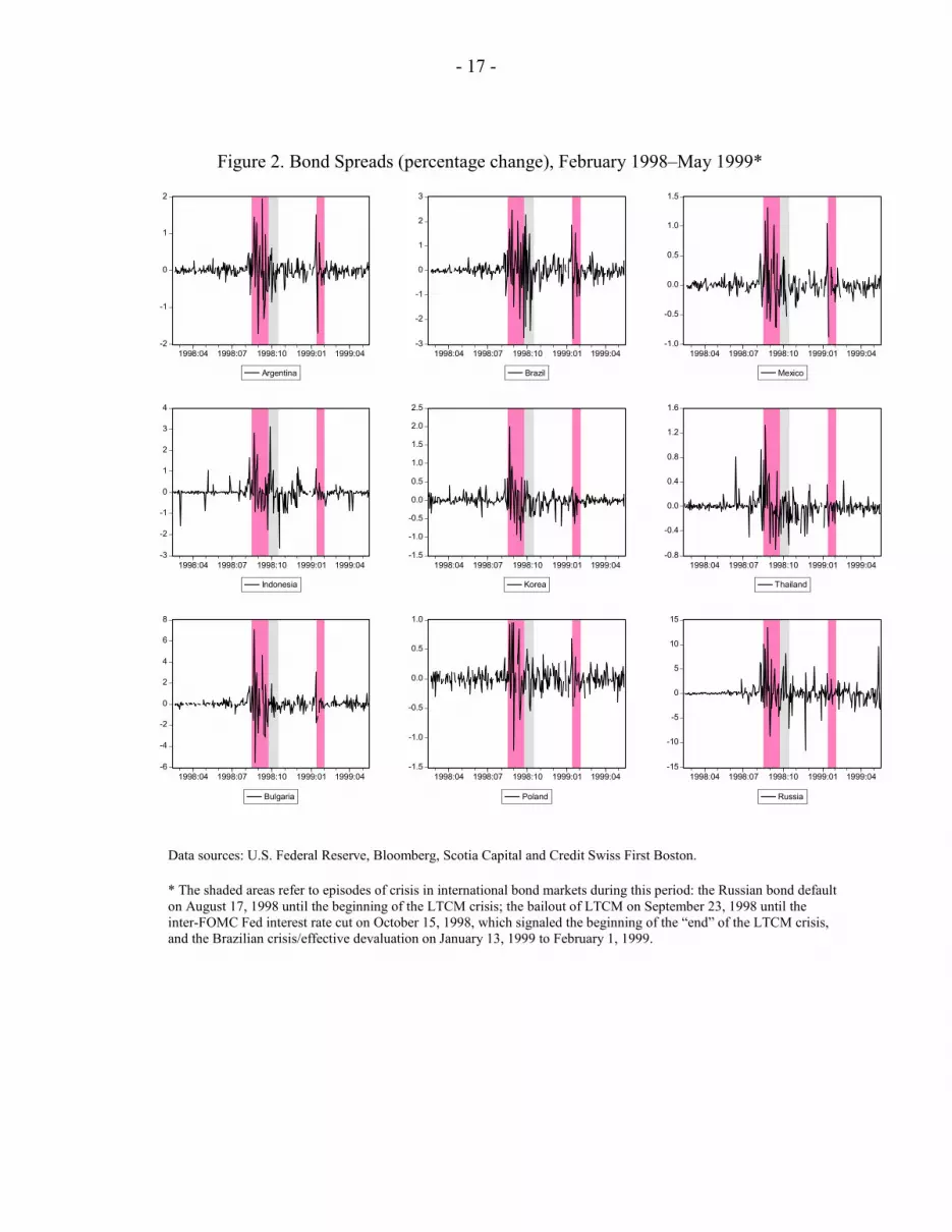
Figure 1 presents the bond spreads in percentage terms for the nine markets studied
over the sample period, whilst Figure 2 presents the same series in changes. The shaded areas highlight the timing of the three crises and the increase in volatility experienced by most of

- 14 -
the markets in the sample over these subperiods.10 Spreads increased during the Russian/LTCM crises in August/September, 1998 (Figure 1). This increase occurs both within the Eastern European region as well as in the Latin American and Asian regions. The Brazilian crisis at the start of 1999 appears less dramatic with the impact tending to be felt more within the Latin American bond markets than within other regions. Of all the emerging market bond markets presented in Figure 1, the Russian bond market behaves differently from the rest as the steep climb in spreads during the time of its own crisis is maintained over most of the crisis periods and only tends to ease off by the second quarter of 1999 where its spread falls from around 60 percent to near 40 percent. The maintenance of relatively high spreads in Russia is in contrast with the bond markets of the other countries presented in Figures 1 and 2 which experience falls fairly soon after the beginning of each crisis.
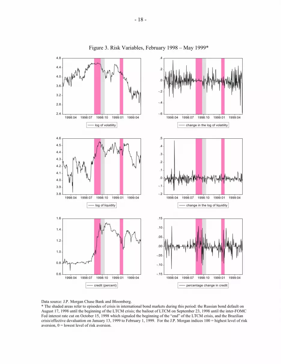
The measures of global risk used in the empirical analysis are based on the risk
components of the J.P. Morgan’s LCVI index of risk aversion. The overall LCVI index is comprised of the weighted average of three risk subcomponents: credit risk, volatility risk and liquidity risk. The three components are assigned equal weights in the index. The volatility risk variable measures are based on the implied volatility of 6 major currencies, the implied volatility of stocks using call and put options on the Chicago Board of Options Exchange, and J.P. Morgan’s global risk appetite index (GRAI) in foreign exchange markets which is based on measures of correlation amongst 15 currencies. The liquidity risk variable is based on the spreads between benchmark and off-the-run U.S. Treasuries across the yield curve, and 10-year U.S. swap spreads. The off-the-run issues are the immediately preceding issues which are effectively the same issues as the benchmark bonds (same credit risk), but are less liquid and tend to enjoy a premium (Greenspan (1999)). Finally, the credit risk variable is based on U.S. corporate high yield B-2 spreads relative to the equivalent U.S. Treasury bond and the EMBI+ which is J.P. Morgan’s measure of credit risk in emerging
10 The exact timing of the crises is an approximation by necessity since in each case pressures began building up before the time at which the crises were revealed to the public. However, the dates chosen follow closely those used in other studies (see, for example, the BIS Committee on the Global Financial System (1999)). Thus, the Russian crisis period is assumed to begin on August 17, 1998 when the country announced its bond default, lasting until the beginning of the LTCM crisis; the LTCM crisis is assumed to begin on September 23, 1998 when the New York Fed orchestrated a rescue plan of LTCM and made the problems of this company public on September 23, 1998, lasting until the inter-FOMC Fed interest rate cut on October 15, 1998 which signaled the beginning of the “end” of the LTCM crisis, according to traders surveyed by the BIS Committee on the Global Financial System (1999); and the Brazilian crisis is assumed to begin with the effective devaluation of the Real on January 13, 1999, lasting for a few weeks during which there were several changes at the top of the central bank until the beginning of February 1999.

- 15 -
markets. An increase in any of these indices represents a move towards a state of increasing risk, whilst a decline in an index is a move towards a lower risk state.11
The J.P. Morgan measures of liquidity and volatility are used directly in the model, and are presented in the first four panels of Figure 3, in terms of the natural logarithm, and the change in the natural logarithm of each variable. However, the J.P. Morgan credit index is not used in the empirical analysis as it includes the J.P. Morgan’s Emerging Market Bond Index (EMBI+), which is essentially highly correlated with the dependent variables of the bond spreads for each emerging economy under investigation. To capture changes in the credit risk of international investors, the U.S. industrial BBB1 10-year corporate bond spread over the comparable U.S. treasury bond is used. This series is presented in the bottom panels of Figure 3, expressed in precentages. This bond spread captures global credit concerns given that international investors are largely U.S. based, or at least use U.S. assets as benchmarks in pricing risks and returns in international financial markets. All three risk variables in Figure 3 indicate a continual increase in risk that begins prior to the Russian/LTCM crises of August/September, 1998, and peaks during this crisis.
Some descriptive statistics of the emerging market bond spreads, and also the three
risk measures are presented in Tables A2.1 to A2.4 in Appendix II. These statistics show that Russia experienced the largest spread over the period of 68.3 percent, followed by Bulgaria (22.8 percent) and Indonesia (18.7 percent). Russia also experienced the largest daily increase in its spread (13.4 percent), again followed by Bulgaria (7.0 percent) and Indonesia (3.1 percent).
The 12-variate VAR in (4) is estimated by maximum likelihood based on equations
(15) and (16). Tables A2.3 and A2.4 highlight the presence of autocorrelation in the movements of the variables which suggests the need for a non-zero lag structure in the VAR. Using information criteria statistics the lag structure is chosen to be L=5.12 The long-run 11 The J.P. Morgan risk components are expressed as indices and are constructed as follows. The raw data underlying each risk measure are initially transformed using a cumulative distribution function. The advantage of this approach is that it does not assume normality and deals with all the moments of the distribution. Each observation is then expressed as a percentile of the distribution function, in a way that a higher level represents more risk, with 0 being the minimum risk and 100 the maximum risk. Finally, an average of resulting comparable units produces a measure of the overall risk variables and its components. For further information on the construction of the LCVI index and its sub-components, see J.P. Morgan (1999) and J.P. Morgan Chase Bank (2002)).
12 Information criteria based on AIC, SIC and HIC statistics were used in conjunction with a likelihood ratio (LR) test to identify the optimal lag structure. A lag length of p=5 lags is based on the AIC and the LR test, whilst the SIC and the HIC identified a lag structure of p=0 lags. Inspection of the t-statistics associated with individual lags suggested that a lag structure of p=5 was more appropriate to model the dynamics of the system.

- 16 -
parameter estimates of (13) are reported in Table A3.1. The parameter estimates of the lags of the variables are not reported. Instead the contribution of these estimates is presented within the historical decomposition results, which is more informative in the present context.
Figure 1. Bond Spreads (percent), February 1998 – May 1999*
3
4
5
6
7
8
9
10
11
1998:04 1998:07 1998:10 1999:01 1999:04
Argentina
4
6
8
10
12
14
16
1998:04 1998:07 1998:10 1999:01 1999:04
Brazil
2
3
4
5
6
7
8
9
1998:04 1998:07 1998:10 1999:01 1999:04
Mexico
4
6
8
10
12
14
16
18
20
1998:04 1998:07 1998:10 1999:01 1999:04
Indonesia
1
2
3
4
5
6
7
8
9
10
1998:04 1998:07 1998:10 1999:01 1999:04
Korea
1
2
3
4
5
6
7
8
9
10
1998:04 1998:07 1998:10 1999:01 1999:04
Thailand
4
8
12
16
20
24
1998:04 1998:07 1998:10 1999:01 1999:04
Bulgaria
1
2
3
4
5
6
1998:04 1998:07 1998:10 1999:01 1999:04
Poland
0
10
20
30
40
50
60
70
1998:04 1998:07 1998:10 1999:01 1999:04
Russia
Data sources: U.S. Federal Reserve, Bloomberg, Scotia Capital and Credit Swiss First Boston.
* The shaded areas refer to episodes of crisis in international bond markets during this period: the Russian bond default on August 17, 1998 until the beginning of the LTCM crisis; the bailout of LTCM on September 23, 1998 until the inter-FOMC Fed interest rate cut on October 15, 1998, which signaled the beginning of the “end” of the LTCM crisis, and the Brazilian crisis/effective devaluation on January 13, 1999 to February 1, 1999.
- 17 -
Figure 2. Bond Spreads (percentage change), February 1998–May 1999*
-2
-1
0
1
2
1998:04 1998:07 1998:10 1999:01 1999:04
Argentina
-3
-2
-1
0
1
2
3
1998:04 1998:07 1998:10 1999:01 1999:04
Brazil
-1.0
-0.5
0.0
0.5
1.0
1.5
1998:04 1998:07 1998:10 1999:01 1999:04
Mexico
-3
-2
-1
0
1
2
3
4
1998:04 1998:07 1998:10 1999:01 1999:04
Indonesia
-1.5
-1.0
-0.5
0.0
0.5
1.0
1.5
2.0
2.5
1998:04 1998:07 1998:10 1999:01 1999:04
Korea
-0.8
-0.4
0.0
0.4
0.8
1.2
1.6
1998:04 1998:07 1998:10 1999:01 1999:04
Thailand
-6
-4
-2
0
2
4
6
8
1998:04 1998:07 1998:10 1999:01 1999:04
Bulgaria
-1.5
-1.0
-0.5
0.0
0.5
1.0
1998:04 1998:07 1998:10 1999:01 1999:04
Poland
-15
-10
-5
0
5
10
15
1998:04 1998:07 1998:10 1999:01 1999:04
Russia
Data sources: U.S. Federal Reserve, Bloomberg, Scotia Capital and Credit Swiss First Boston.
* The shaded areas refer to episodes of crisis in international bond markets during this period: the Russian bond default on August 17, 1998 until the beginning of the LTCM crisis; the bailout of LTCM on September 23, 1998 until the inter-FOMC Fed interest rate cut on October 15, 1998, which signaled the beginning of the “end” of the LTCM crisis, and the Brazilian crisis/effective devaluation on January 13, 1999 to February 1, 1999.
- 18 -
Figure 3. Risk Variables, February 1998 – May 1999*
2.4
2.8
3.2
3.6
4.0
4.4
4.8
1998:04 1998:07 1998:10 1999:01 1999:04
log of volatility
-.6
-.4
-.2
.0
.2
.4
1998:04 1998:07 1998:10 1999:01 1999:04
change in the log of volatility
3.8
3.9
4.0
4.1
4.2
4.3
4.4
4.5
4.6
1998:04 1998:07 1998:10 1999:01 1999:04
log of liquidity
-.2
-.1
.0
.1
.2
.3
.4
.5
1998:04 1998:07 1998:10 1999:01 1999:04
change in the log of liquidity
0.6
0.8
1.0
1.2
1.4
1.6
1998:04 1998:07 1998:10 1999:01 1999:04
credit (percent)
-.15
-.10
-.05
.00
.05
.10
.15
1998:04 1998:07 1998:10 1999:01 1999:04
percentage change in credit
Data source: J.P. Morgan Chase Bank and Bloomberg. * The shaded areas refer to episodes of crisis in international bond markets during this period: the Russian bond default on August 17, 1998 until the beginning of the LTCM crisis; the bailout of LTCM on September 23, 1998 until the inter-FOMC Fed interest rate cut on October 15, 1998 which signaled the beginning of the “end” of the LTCM crisis, and the Brazilian crisis/effective devaluation on January 13, 1999 to February 1, 1999. For the J.P. Morgan indices 100 = highest level of risk aversion, 0 = lowest level of risk aversion.

- 19 -
Table 1: Mean and Standard Deviation of Benchmark Prices Over the Crisis Period, Based on Precrisis Information (percentage points)*
Country Mean Standard deviation Argentina 5.691 0.508 Brazil 6.537 0.667 Mexico 4.050 0.255 Indonesia 7.092 0.031 Korea, Rep. of 4.141 0.217 Thailand 2.619 0.270 Bulgaria 8.793 1.030 Poland 2.226 0.099 Russia 20.943 7.953
* The crises period is assumed to begin June 1, 1998 and end May 17, 1999
A. Benchmark Prices Based on Precrisis Information
Table 1 presents summary statistics on the benchmark prices (the conditional
forecasts) of each country over the crisis period as defined in (17). The market fundamentals are based on starting the historical decomposition on June 1, 1998, which occurs before the beginning of the Russian crisis and is assumed to be the beginning of the crises period.13 With the exception of Russia, the sample means of the benchmark price for most countries range between 2 and 8 percent over the crisis period. The Republic of Poland has the smallest mean of around 2 percent, which is consistent with the actual bond spreads over the pre-crisis periods as presented in Figure 1. The mean estimate for Russia is the highest, with a value of 21 percentage points. This reflects relatively high spreads sustained in the Russian bond 13 For purposes of the empirical estimation, the period of crises is assumed to begin after June 1, 1998 or a few months before the actual disclosure of Russia’s default on August 17, 1998, and last until a few months after the worst of the turmoil appeared to have ended in Brazil after the speculative attack of the Real in January 1999. The crises period assumed for the empirical estimation is purposely longer than the anecdotal public information disclosure and is based on the observation of when markets were relatively calm before the announcement of the various crises. This guarantees that our period of non-crises corresponds to the period in which markets were quite stable and attempts to deal with the fact that crises almost never begin when they become publicly known but pressures typically mount before the news event.

- 20 -
market over the crisis period. A comparison of the mean of the benchmark prices given in Table 1 with those for the raw spreads data given in Table II.1, shows that the mean of the benchmark prices is lower than those of the actual data for all countries with the exception of Argentina, where the differences between the two means is numerically small. This result shows, in general, that the unexpected shocks experienced during the crisis period contributed to higher-than-expected spreads when compared with levels based on precrisis information.
The estimates of the benchmark prices at each point in time over the crisis periods for
each of the nine countries studied, are presented in the first panel of Figures 4 to 12. For all countries with the exception of those from Asia, the benchmark prices on average steadily increase over the period of the historical decomposition. In particular, the benchmark prices of Russia deteriorate markedly from around 6.5 percent on June 1, 1998 to 35 percent on May 17, 1999. As noted above, this reflects the sustained level of spreads experienced in the Russian bond market over the crisis period with very little reversion back to pre-crisis levels. The benchmark prices of the Asian countries either tend to be relatively flat over the period (Indonesia), or show a slight fall over the period (the Republic of Korea and Thailand). This last feature of the benchmark prices reflects the Republic of Korea’s and Thailand’s recovery from their own financial crises that began in July 1997, as well as the stabilization in Indonesia, which was the slowest of the Asian economies to recover from the Asian crisis.
B. Risk Factors
Figures 4 to 12 provide the results of the historical decompositions of the risk premia
of the nine emerging markets. On each day, the actual bond spread is decomposed into (a) the benchmark level; (b) the three components representing shocks in global risk (volatility, liquidity, and credit); (c) country risk; and (d) risk from contagion corresponding to the contribution of shocks from the bond markets of emerging markets in the Asian, Latin America, and Eastern European regions. The average decomposition of the risk premia of each country are summarized in Table 2 for each of the three crises.
Latin America
Figures 4 to 6 provide the results of the historical decomposition of the percentage bond spreads over the crisis periods for the Latin American countries of Argentina, Brazil, and Mexico respectively. An interesting feature of all three risk components, is that they exhibit quite similar characteristics over the crisis period for all Latin American countries. On average, the contribution of credit risk is relatively higher than either volatility or liquidity risks for all Latin American countries during the Russian and LTCM crises. The importance of credit risk to Latin America is evident during the Russian crisis where its contribution to bond spreads jumps during the period by about 1.5 percent. During the Brazilian crisis the contribution of credit risk to the overall risk premium however falls from its historical high, resulting in similar contributions across the three components of risk to overall risk. For example, from Table 2, the contributions range from 0.35 to 0.48 percent for Argentina, 0.57 to 0.70 percent for Brazil and 0.26 to 0.36 percent for Mexico. Country-

- 21 -
specific risk is also important for most of the Latin American economies, especially in the case of Brazil and Mexico. The contribution contagion risk arising from shocks in the bond spreads from the other emerging bond markets over the crisis period are relatively small, and do not appear to exhibit a clear systematic pattern in explaining Latin American bond spreads.
An interesting feature of the contribution of shocks to volatility and credit to bond
risk premia highlighted in Figures 4 to 6 is that they exhibit two humps: one corresponding to the Russian/LTCM crisis, followed by another in the period building up to the Brazilian speculative attack in January 1999 for the case of volatility, and just after the Brazilian crisis for credit risk. In contrast, the contribution of liquidity risk to Latin American bond spreads does not decline over the period between the LTCM crisis and the Brazilian crisis. Rather, it is not until about a month after the Brazilian crisis that the contribution of liquidity risk to bond spreads in Latin America abate. The increase in the contribution of volatility risk to bond spreads in Latin America occurs well before the speculative attack materialized in January 1999. This is despite the fact that Brazil was in the midst of program negotiations with the IMF during the last few months of 1998. Brazil presented a formal letter of intent to the IMF on November 13, 1998 and a program was approved on December 2, 1998. In fact, the second hump in volatility risk begins in December around the time of the IMF approval. These results are consistent with the view that Brazil was affected by contagion from the previous Russian and LTCM crises (Baig and Golfjan (2000)). In fact, there is evidence that the Russian crisis had a particularly important effect on Brazil’s bond spreads (Dungey, Fry, González-Hermosillo and Martin (2000a, b)) while the LTCM shock had an important impact on Brazil’s equity markets (Dungey, Fry, González-Hermosillo and Martin (2003)).
Asia
The decomposition of Asian bond spreads for Indonesia, the Republic of Korea and
Thailand are given in Figures 7 to 9 respectively. For the three specific crises investigated over the period, the mean decompositions of the bond spreads are summarized in Table 2. The overall contribution of the three global risk factors to bond spreads for the Asian economies exhibit qualitatively similar patterns to the three Latin American countries. In particular, there are two humps in volatility, one corresponding to the Russian crisis and one occurring just prior to the Brazilian crisis. Shocks in liquidity risk exhibit a jump during the Russian crisis which does not subside until a month after the Brazilian crisis, whilst shocks in credit risk contribute to the widening of bond spreads during the Russian crisis, subsides following the LTCM crisis and peaks again locally just following the Brazilian crisis. The major source of improvement in bond spreads for the Asian economies over the crisis period stems from country specific risk associated with each country following the Russian crisis. This may reflect the improvement of the Asian economies in the post-Asian crisis period, indicating that credit concerns were becoming less of an issue for these economies compared to the pre-crisis period. The relative importance of the credit risk and the volatility risk components is generally higher than liquidity risk for most Asian economies over the three crises. Further, and as with the Latin American countries, there is very little evidence of contagion arising from the transmission of unanticipated shocks across national bond markets.

- 22 -
Table 2. Mean Decomposition of Spreads During Each Crisis
Country Actual Bench. Volatility Liquidity Credit Country Asia Lat. Am. Europe
Argentina Russian crisis 1 8.07 5.30 0.43 0.52 1.04 0.63 0.00 0.19 -0.03 LTCM crisis 2 6.48 5.45 0.34 0.58 1.35 -1.35 0.13 -0.09 0.08 Brazilian crisis 3 7.04 6.00 0.35 0.48 0.44 -0.52 0.06 0.24 0.00
Brazil Russian crisis 11.67 6.02 0.72 0.76 1.71 2.35 -0.01 0.13 -0.02 LTCM crisis 11.52 6.22 0.54 0.84 2.13 1.53 0.12 0.12 0.01 Brazilian crisis 11.78 6.94 0.57 0.70 0.64 2.98 0.06 -0.08 -0.04 Mexico Russian crisis 7.06 3.86 0.32 0.33 0.95 1.65 -0.03 0.00 0.00 LTCM crisis 6.97 3.93 0.25 0.37 1.19 1.11 0.07 0.04 0.01 Brazilian crisis 5.95 4.20 0.26 0.30 0.36 0.88 0.02 -0.04 -0.03 Indonesia Russian crisis 15.03 7.12 1.05 0.07 1.21 5.71 -0.08 -0.02 -0.03 LTCM crisis 16.56 7.11 0.81 0.10 1.38 7.05 0.09 -0.08 0.09 Brazilian crisis 11.29 7.08 0.83 0.08 0.32 3.07 -0.05 0.01 -0.05 Korea Russian crisis 8.12 4.32 0.80 0.30 0.82 1.83 -0.04 0.10 -0.01 LTCM crisis 7.01 4.25 0.61 0.34 0.93 0.66 0.10 0.04 0.07 Brazilian crisis 3.34 4.01 0.63 0.28 0.21 -1.77 -0.03 0.04 -0.02 Thailand Russian crisis 7.69 2.84 0.85 0.32 0.75 2.90 -0.04 0.05 0.02 LTCM crisis 6.13 2.76 0.64 0.36 0.92 1.31 0.08 0.04 0.02 Brazilian crisis 3.01 2.46 0.67 0.29 0.27 -0.66 -0.04 0.01 0.01 Bulgaria Russian crisis 18.50 8.01 2.36 1.02 1.85 4.87 0.04 0.38 -0.04 LTCM crisis 13.56 8.31 1.77 1.12 2.12 -0.42 0.11 0.32 0.21 Brazilian crisis 11.23 9.41 1.84 0.93 0.50 -1.61 0.14 0.01 0.00 Poland Russian crisis 3.69 2.15 0.30 0.18 0.18 0.77 0.02 0.09 0.00 LTCM crisis 3.57 2.18 0.22 0.20 0.16 0.73 0.03 0.06 -0.01 Brazilian crisis 3.29 2.28 0.23 0.16 -0.01 0.66 -0.01 -0.01 -0.02 Russia Russian crisis 55.19 14.76 4.73 2.92 15.35 18.28 0.14 -0.33 -0.66 LTCM crisis 59.89 17.15 3.60 3.30 20.21 14.40 1.02 0.19 0.02 Brazilian crisis 51.45 25.71 3.76 2.71 6.96 12.75 0.58 -0.50 -0.53 1 Russian crisis: August 27-September 22, 1998. 2 LTCM crisis: September 23-October 15, 1998. 3 Brazilian crisis: January 13-February 2, 1999.

- 23 -
Eastern Europe
The decomposition of bond spreads for the Eastern European countries of Bulgaria, the Republic of Poland and Russia are given in Figures 10 to 12 respectively, with the mean decompositions corresponding to the three crises summarized in Table 2. These results show that the contributions of the risk factors to bond spreads in Eastern Europe exhibit similar patterns to the Latin American and Asian regions. The credit component of risk has the greatest absolute effect on Russia of all the emerging market countries investigated, adding on average, 15% to the risk premium during the Russian crisis, 20% during the LTCM crisis and 7% during the Brazilian crisis. The contributions of volatility and liquidity risk shocks are relatively smaller, but nonetheless important, adding between 3% and 5% to the risk premium during all three crises. The relative importance of country specific risk, especially during the Russian crisis, suggests that the Russian crisis was idiosyncratic, being a function largely of its own internal dynamics. However, the relative importance of the credit factor in contributing to bond spreads reflects the crisis as being more a crisis of credit. This is consistent given that the Russian government defaulted on its loans. As with the Latin American and Asian countries, there is little evidence of contagion connecting national bond markets both within the Eastern European region and outside this region.
IV. CONCLUSIONS AND SUGGESTIONS FOR FUTURE RESEARCH
A channel for the transmission of crises that has become increasingly important in financial market and policy circles relates to international investors’ appetite for risk (see, for example, J.P. Morgan, 1999, and International Monetary Fund, 2002, 2003a, 2003b). The anecdotal evidence suggests that periods of reduced appetite for risk often coincide with periods of distress across global financial markets. Russia’s default in August 1998 and the near-collapse of the U.S. highly leveraged hedge fund, Long-Term Capital Management (LTCM), in September 1998 appear to be such examples. The Brazilian financial crisis in late 1998 and early 1999 when the real was devalued was also felt in a number of countries, especially in Latin America. The aim of this paper was to identify the role of changes in the risk appetite of investors in mature financial markets in determining sovereign bond spreads issued by emerging markets. Three components of global risk were investigated: volatility risk, as measured by implied volatilities in currency and equity options markets; credit risk which was based on the spreads on high-yield B-2 bonds in the U.S.; and liquidity risk, which was proxied by the liquidity premium between on-the-run and off-the-run U.S. treasury bonds. The role of country risk and contagion risk in contributing to changes in the risk premia of emerging markets were also investigated. Using a structural vector autoregression model, a historical decomposition of the risk premia of nine emerging markets during 1998–99 was performed. This period included three financial crises; the Russian default of August 1998, the LTCM near-collapse of September 1998, and the crisis in the Brazilian real in January 1999. A feature of the historical decomposition was the identification of a set of benchmark prices for each emerging market,

- 24 -
which was used to provide an estimate of spreads in the event of no crises. The difference between the actual and benchmark values were then decomposed into the various components of risk, including the three global risk factors, country risk, and contagion risk. The empirical results showed that the increase in risk premia in most countries during the Russian/LTCM crises arose from a combination of increasing credit risk and country risk. The importance of the credit risk component during the Russian crisis, in particular, is consistent with the view that this was a global credit risk shock. Risk from volatility and liquidity were found to be relatively smaller. In contrast, the contributions of the three risk components to bond spreads during the Brazilian crisis tended to be similar with some variations across regions. Overall, the results suggest that different characterizations of global risk patterns were at play during the recent financial crises analyzed in this paper. However, country-specific risk also contributed importantly to the bond spreads, indicating that the higher cost of borrowing for emerging markets in international financial markets was not solely related to heightened global risk. Finally, there was very little evidence of contagion arising from shocks in bond markets across national borders.
Some extensions of the modeling framework presented here could be entertained in
the following ways. The modeling framework proposed represented a multifactor asset- pricing model for emerging bond markets where the pertinent shocks arose from unanticipated movements in liquidity, credit, and volatility risk of developed markets, as well as unanticipated movements in the risk premia of other emerging markets. The types of shocks studied could be expanded by including a set of common shocks to produce a multifactor capital asset pricing model along the lines of Bekeart, Harvey, and Ng (2003). Alternatively, the common shocks could be identified implicitly following the approach of Dungey, Fry, and Martin (2003). An expanded set of variables could also be included in the VAR to capture the market fundamentals underlying the risk premia of the emerging markets. This would have the advantage that the benchmark prices computed over the crisis period could also be interpreted as the market fundamental prices. Further refinements of the model could be along the lines of allowing for a time-varying volatility structure. The multivariate GARCH class of models is an obvious choice, although issues of dimension arise immediately. One solution is to adopt a factor GARCH structure and allow for a low dimensional set of second moment dynamics through the underlying factors following the work of Dungey, Fry, González-Hermosillo, and Martin (2002a). Finally, a historical decomposition of the risk indices themselves could be constructed to understand the contribution of shocks in emerging markets and other risk indices to global investor risk preferences.
One further extension that could be contemplated would be to decompose the mean
spread in terms of the the product of the quantity of risk and the price of risk of the various components of the VAR, including the risk variables that measure volatility, liquidity, and credit. For the case of Epstein-Zin utility functions, which allow for nonseparability across states of nature, the quantity of risk is is the covariance between the spread and the shock in the risk variables and the price of risk is a function of the relative risk aversion parameter (Campbell, 1996). If the covariances are taken as the long-run second moments, the

- 25 -
calculation of the prices of risk associated with the shocks in the three risk variables could then be computed using the approach of Cochrane and Piazzesi (2001). Alternatively, if a time-varying covariance model was estimated along the lines suggested above, then it would be possible to perform these calculations at each point in time and identify changes in the relative risk aversion parameter during the crisis periods. Identification of potentially significant structural breaks in risk aversion could then be based on the methods of Andrews (1993), Andrews and Ploberger (1994), and Hansen (1997, 2000).

- 26 - APPENDIX I
Data Definitions and Sources
Sample Period: February 12, 1998 to May 17, 1999, (328 observations). 1. Risk Aversion Variables LCVI Liquidity Index: J.P. Morgan Chase Bank’s liquidity index. The index ranges from zero
(low risk) to 100 (high risk). Source: J.P. Morgan Chase Bank. Components:
US Treasury yield spreads of benchmark and off-the-run bonds for different maturities.
10-year US swap spreads.
LCVI Volatility Index: J.P. Morgan Chase Bank’s volatility index. The index ranges from zero (low risk) to 100 (high risk).
Source: J.P. Morgan Chase Bank. Components:
Implied 12-month foreign exchange volatility for six currencies (EUR, JPY, CHF, GBP, CAD, AUD against the USD).
Implied equity volatility based on option markets on the Chicago Board of Options Exchange.
J.P. Morgan Global Risk Appetite Index (GRAI) based on measures of correlation between the rank of the $ returns of 15 currencies of the past two months, and the rank of risk measured by historical yield.
Credit: U.S. Industrial BBB1 Corporate 10-year Bond Spread over U.S. Treasury. Spread
expressed in percentage. Source: Bloomberg (IN10Y3B1).
2. Bond Spreads Argentina: Republic of Argentina bond spread over U.S. Treasury. Source: U.S. Federal Reserve. Brazil: Republic of Brazil bond spread over U.S. Treasury. Source: U.S. Federal Reserve.
Mexico: J.P. Morgan Eurobond Index Mexico Sovereign spread over U.S. Treasury. Source: U.S. Federal Reserve.
Indonesia: Indonesian Yankee Bond Spread over U.S. Treasury. Source: U.S. Federal Reserve.

- 27 - APPENDIX I
Republic of Korea: Government of Korea 8 7/8% 4/2008 over U.S. Treasury. Source: U.S. Federal Reserve.
Thailand: Kingdom of Thailand Yankee Bond Spread over U.S. Treasury.
Source: U.S. Federal Reserve.
Bulgaria: Bulgarian Discount Stripped Brady Bond Yield Spread over U.S. Treasury. Source: U.S. Federal Reserve.
Republic of Poland: Poland Par Stripped Brady Bond Yield Spread over U.S. Treasury. Source: U.S. Federal Reserve.
Russia: Government of Russia 9.25% 11/2001 over U.S. Treasury. Source: Bloomberg (007149662).
The bond spreads, or “risk premiums,” are constructed by taking a representative long-term sovereign bond issued in U.S. dollars by an emerging country and subtracting from it a U.S. treasury bond of comparable maturity. For the United States, the risk premium is constructed by taking a representative long-term corporate bond in domestic currency and subtracting from it a government treasury bond of comparable maturity. All bond spreads are expressed as a percentage. Missing observations are dealt with by replacing the missing value with the previous day’s observation.


Ta
ble
A3.
1. L
ong-
Run
Par
amet
er E
stim
ates
of H
in
(13)
Dep
ende
nt V
aria
bles
E
xpla
nato
ry
Var
iabl
es
Vol
atili
ty
Liq
uidi
ty
Cre
dit
Arg
entin
a B
razi
l M
exic
o In
done
sia
Kor
ea
Tha
iland
B
ulga
ria
Pola
nd
Rus
sia
Vol
atili
ty
0.06
0.
03
0.06
0.
02
0.18
0.
02
0.37
0.
08
0.06
0.
07
Liqu
idity
0.03
0.06
0.
09
0.04
0.
13
0.02
0.
36
0.01
0.
04
0.04
C
redi
t
0.
03
0.08
0.
13
0.07
0.
13
0.01
1.
26
0.09
0.
06
0.06
A
rgen
tina
0.
30
Bra
zil
0.39
Mex
ico
0.
20
Indo
nesi
a
0.
83
K
orea
0.15
Th
aila
nd
2.31
- 30 -
Bul
garia
0.58
Po
land
0.
31
R
ussi
a
0.26
APPENDIX III

- 31 -
References
Andrews, Donald W.K., 1993, “Tests for Parameter Instability and Structural Change with
Unknown Change Point,” Econometrica (July), pp. 821–56. ———, and Werner Ploberger, 1994, “Optimal Tests when a Nuisance Parameter is Present
Only under the Alternative,” Econometrica (November), pp. 1383–1414. Bae, Kee-Hong, George A. Karyoli, and Rene M. Stulz, 2003, “A New Approach to Measuring
Financial Contagion,” Review of Financial Studies, forthcoming. Bank of England, 2002, Financial Stability Review, London, England, June 2002. Bekaert, Geert, Campbell R. Harvey, and Angela Ng, 2003, “Market Integration and
Contagion,” Journal of Business, forthcoming. Blanchard, Olivier Jean, and Danny Quah, 1989, “Aggregate Demand and Supply
Disturbances,” American Economic Review, 1989, Vol. 83(3), pp. 655–73. Breeden, Douglas T., 1979, “An Intertemporal Asset Pricing Model with Stochastic
Consumption and Investment Opportunities,” Journal of Financial Economics, 7 pp. 265–96.
Calvo, Gillermo A. and Enrique G. Mendoza, 2000, “Rational Contagion and the Globalization
of Securities Markets,” Journal of International Economics, Vol. 51(1), pp. 9–113. Campbell, John, 1996, “Understanding Risk and Return,” Journal of Political Economy,
Vol. 104(2), pp. 298–345. Cochrane, John, 2001, Asset Pricing, Princeton University Press. ———, and Monika Piazzesi, 2001, “Bond Risk Premia,” (unpublished). Committee on the Global Financial System, 1999, A Review of Financial Market Events in
Autumn 1998 (Basel, Switzerland: Bank for International Settlements) October. Diamond, Douglas W., and Philip H. Dybvig, 1983, “Bank Runs, Deposit Insurance, and Liquidity,” The Journal of Political Economy, Vol. 91, pp. 401–19. Dornbusch, Rudiger, Yung C. Park, and Stijn Claessens, 2000, “Contagion: Understanding
How It Spreads,” World Bank Research Observer, Vol. 15 (August), pp. 177–97.

- 32 -
Dungey, Mardi, Renée Fry, Brenda González-Hermosillo, and Vance L. Martin, 2002a, “International Contagion Effects from the Rusian Crisis and the LTCM Near-Collapse,” IMF Working Paper 02/74 (Washington: International Monetary Fund).
___________ (2002b), “The Transmission of Contagion in Developed and Developing
International Bond Markets,” in Risk Measurement and Systemic Risk (Basel Switzerland: Bank for International Settlements).
___________ (2003), “Unanticipated Shocks and Systemic Influences: The Impact of
Contagion in Global Equity Markets in 1998,” IMF Working Paper 03/84 (Warhington: International Monetary Fund).
Dungey, Mardi, Renée Fry, and Vance L. Martin, 2003, “Identification of Common and
Idiosyncratic Shocks in Real Equity Prices: Australia, 1982 to 2002,” Australian National University Working Paper in Trade and Development 2003/18.
Eichengreen, Barry, Andrew K. Rose, and Charles Wyplosz, 1996, “Contagious Currency
Crises,” NBER Working Paper No. 5681 (Cambridge, Massachusetts: National Bureau of Economic Research).
Forbes, Kristin, 2001, “Are Trade Linkages Important Determinants of Country Vulnerability to
Crises,” NBER Working Paper No. 8194 (Cambridge, Massachusetts: National Bureau of Economic Research).
———, and Roberto Rigobon, 2002, “No Contagion, Only Interdependence: Measuring Stock
Market Co-Movement,” Journal of Finance, Vol. 57(5), pp. 2223–61. Gertler, Mark, and Cara Lown, 2000, “The Information in the High-Yield Bond Spread for the
Business Cycle: Evidence and Some Implications,” NBER Working Paper No. 7549 (Cambridge, Massachusetts: National Bureau of Economic Research).
Glick, Reuven, and Andrew K. Rose, 1999, “Contagion and Trade: Why are Currency Crises
Regional,” Journal of International Money and Finance, Vol. 8, pp. 603–17. Goldfajn, Ilan, and RodrigoValdes, 1997, “Capital Flows and the Twin Crises: The Role of
Liquidity,” IMF Working Paper 97/87 (Washington: International Monetary Fund). Goldstein, Morris, 1998, The Asian Financial Crisis: Causes, Cures and Systemic Implications,
Policy Analysis in International Economics, No. 55 (Washington: Institute for International Economics).
Greenspan, Alan, 1999, “Risk, Liquidity and the Economic Outlook,” Business Economics,
January, pp. 20–24.

- 33 -
Grossman, Sanford J., and Robert J. Shiller, 1981, “The Determinants of the Variability of Stock Market Prices,” American Economic Review, Vol. 71, pp. 222–27.
Hamilton, James, 1994, Time Series Analysis, Princeton University Press, Princeton, New
Jersey. Hansen, Bruce E., 1997, “Approximate Asymptotic p-values for Structural Change Tests,”
Journal of Business and Economic Statistics, Vol. 15, p. 67. ———, 2000, “Testing for Structural Change in Conditional Models,” Journal of
Econometrics, 2000, Vol. 97, pp. 93–115. International Monetary Fund, 2002, Global Financial Stability Report: Market Developments
and Issues (Washington) September. ———, 2003a, Global Financial Stability Report: Market Developments and Issues
(Washington) March. ———, 2003b, Global Financial Stability Report: Market Developments and Issues
(Washington) September. Jorion, Philippe, 2000, “Risk Management Lessons from Long-Term Capital Management,”
European Financial Management, Vol. 6 (September), pp. 277–300 J.P. Morgan, 1999, “Introducing Our New Liquidity and Credit Premia Update,” Global FX and
Precious Metals Research, New York, August 25, 1999. J.P. Morgan Chase Bank, 2002, “Using Equities to Trade FX: Introducing the LCVI,” Global
Foreign Exchange Research, New York, October 1, 2002. Kaminsky, Graciela L., and Carmen M. Reinhart, 2002, “The Center and the Periphery: The
Globalization of Financial Turmoil,” paper presented at the Third Joint Central Bank Research Conference on Risk Measurement and Systemic Risk, 7-8 March 2002 (Basel, Switzerland: Bank for International Settlements).
Kaminsky, Graciela L., and Sergio Schmukler, 1999, “What Triggers Market Jitters? A
Chronicle of the Asian Crisis,” Journal of International Money and Finance, Vol. 18(4) August, pp. 537–60.
Kodres, Laura E., and Matthew Pritsker, 2002, “A Rational Expectations Model of Financial
Contagion,” Journal of Finance, Vol. 57(April), pp. 768–99. Kruger, Mark, Patrick N. Osakwe, and Jennifer Page, 1998, “Fundamentals, Contagion and
Currency Crises: An Empirical Analysis,” Bank of Canada Working Paper #98-10.

- 34 -
Kumar, Manmohan, and Avinash Persaud, 2001, “Pure Contagion and Investors’ Shifting Risk Appetite: Analytical Issues and Empirical Evidence,” IMF Working Paper 01/134 (Washington: International Monetary Fund).
Lintner, John, 1965, “Security Prices, Risk and Maximal Gains from Diversification,” Journal
of Finance, Vol. 20, pp. 587–615. Masson, Paul, 1999a, “Multiple Equilibria, Contagion and the Emerging Market Crises,” IMF
Working Paper 99/164 (Washington: International Monetary Fund). ———, 1999b, “Contagion: Monsoonal Effects, Spillovers, and Jumps Between Multiple
Equilibria,” in The Asian Financial Crisis: Causes, Contagion and Consequences ed. by Pierre-Richard Agenor, Marcus Miller, David Vines, and Axel Weber (Cambridge, U.K.: Cambridge University Press) pp. 265–83.
———, 1999c, “Multiple Equilibria, Contagion and the Emerging Market Crises,” IMF
Working Paper 99/164 (Washington: International Monetary Fund). Missina, Miroslav, 2003, “What Does the Risk-Appetite Index Measure,” Bank of Canada
Working Paper 2003-23 (Ottawa: Bank of Canada), August. Mody, Ashoka, and Mark P. Taylor, 2002, “Forecasting US Economic Activity: The High Yield Spread Versus the Term Spread,” (unpublished; Washington: International
Monetary Fund). ———, 2003, “Common Vulnerabilities,” (unpublished; University of Warwick). Peck, James, and Karl Shell, 2003, “Equilibrium Bank Runs,” The Journal of Political
Economy, Vol. 111, pp. 103–23. Pesaran, M. Hashem, and Yongcheol Shin, 1998, “Generalised Impulse Response Analysis in
Linear Multivariate Models,” Economics Letters, Vol. 58(1), pp. 17–29. Sharpe, William, 1964, “Capital Asset Prices: A Theory of Market Equilibrium Under
Conditions of Risk,” Journal of Finance, Vol. 19, pp. 425–42. Schinasi, Garry, and Todd Smith, 1999, “Portfolio Diversification, Leverage, and Financial
Contagion,” IMF Working Paper 99/136 (Washington: International Monetary Fund). Solnik, Bruno H., 1974, “An Equilibrium Model of the International Capital Market,” Journal
of Economic Theory, Vol. 8, pp. 500–24. Van Rijckeghem, Caroline, and Beatrice Weder, 2000, “Spillovers Through Banking Centers: A
Panel Data Analysis,” IMF Working Paper 00/88 (Washington: International Monetary Fund).

- 35 -
Figure 4. Decomposition of Bond Spreads – Argentina (June 1, 1998 - May 17, 1999)
4
5
6
7
8
9
10
11
1998:07 1998:10 1999:01 1999:04
actual benchmark
-.2
-.1
.0
.1
.2
.3
.4
.5
1998:07 1998:10 1999:01 1999:04
volatility
-.4
-.2
.0
.2
.4
.6
.8
1998:07 1998:10 1999:01 1999:04
liquidity
-0.4
0.0
0.4
0.8
1.2
1.6
2.0
1998:07 1998:10 1999:01 1999:04
credit
-3
-2
-1
0
1
2
3
1998:07 1998:10 1999:01 1999:04
country
-0.8
-0.4
0.0
0.4
0.8
1.2
1998:07 1998:10 1999:01 1999:04
Latin America
-1.0
-0.5
0.0
0.5
1.0
1.5
2.0
1998:07 1998:10 1999:01 1999:04
Asia
-2.0
-1.5
-1.0
-0.5
0.0
0.5
1.0
1.5
1998:07 1998:10 1999:01 1999:04
Europe
-2
0
2
4
6
8
10
12
1998:07 1998:10 1999:01 1999:04
actual total risk

- 36 -
Figure 5. Decomposition of Bond Spreads – Brazil (June 1, 1998 - May 17, 1999)
4
6
8
10
12
14
16
1998:07 1998:10 1999:01 1999:04
actual benchmark
-0.4
-0.2
0.0
0.2
0.4
0.6
0.8
1.0
1998:07 1998:10 1999:01 1999:04
volatility
-0.8
-0.4
0.0
0.4
0.8
1.2
1998:07 1998:10 1999:01 1999:04
liquidity
-0.5
0.0
0.5
1.0
1.5
2.0
2.5
3.0
1998:07 1998:10 1999:01 1999:04
credit
-3
-2
-1
0
1
2
3
4
5
6
1998:07 1998:10 1999:01 1999:04
country
-1.2
-0.8
-0.4
0.0
0.4
0.8
1.2
1998:07 1998:10 1999:01 1999:04
Latin America
-2.0
-1.5
-1.0
-0.5
0.0
0.5
1.0
1.5
1998:07 1998:10 1999:01 1999:04
Asia
-2.0
-1.5
-1.0
-0.5
0.0
0.5
1.0
1.5
1998:07 1998:10 1999:01 1999:04
Europe
-4
0
4
8
12
16
1998:07 1998:10 1999:01 1999:04
actual total risk

- 37 -
Figure 6. Decomposition of Bond Spreads – Mexico (June 1, 1998 - May 17, 1999)
3
4
5
6
7
8
9
1998:07 1998:10 1999:01 1999:04
actual benchmark
-.2
-.1
.0
.1
.2
.3
.4
1998:07 1998:10 1999:01 1999:04
volatility
-.3
-.2
-.1
.0
.1
.2
.3
.4
.5
1998:07 1998:10 1999:01 1999:04
liquidity
-0.4
0.0
0.4
0.8
1.2
1.6
1998:07 1998:10 1999:01 1999:04
credit
-2
-1
0
1
2
3
1998:07 1998:10 1999:01 1999:04
country
-.8
-.4
.0
.4
.8
1998:07 1998:10 1999:01 1999:04
Latin America
-.5
-.4
-.3
-.2
-.1
.0
.1
.2
.3
.4
1998:07 1998:10 1999:01 1999:04
Asia
-2.0
-1.5
-1.0
-0.5
0.0
0.5
1.0
1998:07 1998:10 1999:01 1999:04
Europe
-2
0
2
4
6
8
10
1998:07 1998:10 1999:01 1999:04
actual total risk

- 38 -
Figure 7. Decomposition of Bond Spreads – Indonesia (June 1, 1998 - May 17, 1999)
6
8
10
12
14
16
18
20
1998:07 1998:10 1999:01 1999:04
actual benchmark
-0.4
0.0
0.4
0.8
1.2
1.6
1998:07 1998:10 1999:01 1999:04
volatility
-.15
-.10
-.05
.00
.05
.10
.15
.20
1998:07 1998:10 1999:01 1999:04
liquidity
-0.4
0.0
0.4
0.8
1.2
1.6
2.0
1998:07 1998:10 1999:01 1999:04
credit
-4
-2
0
2
4
6
8
10
12
1998:07 1998:10 1999:01 1999:04
country
-1.2
-0.8
-0.4
0.0
0.4
0.8
1998:07 1998:10 1999:01 1999:04
Latin America
-1.2
-0.8
-0.4
0.0
0.4
0.8
1.2
1998:07 1998:10 1999:01 1999:04
Asia
-3
-2
-1
0
1
2
1998:07 1998:10 1999:01 1999:04
Europe
-4
0
4
8
12
16
20
1998:07 1998:10 1999:01 1999:04
actual total risk

- 39 -
Figure 8. Decomposition of Bond Spreads – Republic of Korea (June 1, 1998 - May 17, 1999)
1
2
3
4
5
6
7
8
9
10
1998:07 1998:10 1999:01 1999:04
actual benchmark
-0.4
-0.2
0.0
0.2
0.4
0.6
0.8
1.0
1998:07 1998:10 1999:01 1999:04
volatility
-.2
-.1
.0
.1
.2
.3
.4
1998:07 1998:10 1999:01 1999:04
liquidity
-0.4
-0.2
0.0
0.2
0.4
0.6
0.8
1.0
1.2
1998:07 1998:10 1999:01 1999:04
credit
-4
-3
-2
-1
0
1
2
3
4
1998:07 1998:10 1999:01 1999:04
country
-.8
-.6
-.4
-.2
.0
.2
.4
.6
1998:07 1998:10 1999:01 1999:04
Latin America
-.6
-.4
-.2
.0
.2
.4
.6
.8
1998:07 1998:10 1999:01 1999:04
Asia
-1.2
-0.8
-0.4
0.0
0.4
0.8
1998:07 1998:10 1999:01 1999:04
Europe
-2
0
2
4
6
8
10
1998:07 1998:10 1999:01 1999:04
actual total risk

- 40 -
Figure 9. Decomposition of Bond Spreads – Thailand (June 1, 1998 - May 17, 1999)
1
2
3
4
5
6
7
8
9
10
1998:07 1998:10 1999:01 1999:04
actual benchmark
-0.4
-0.2
0.0
0.2
0.4
0.6
0.8
1.0
1998:07 1998:10 1999:01 1999:04
volatility
-.3
-.2
-.1
.0
.1
.2
.3
.4
.5
1998:07 1998:10 1999:01 1999:04
liquidity
-0.2
0.0
0.2
0.4
0.6
0.8
1.0
1.2
1998:07 1998:10 1999:01 1999:04
credit
-2
-1
0
1
2
3
4
5
1998:07 1998:10 1999:01 1999:04
country
-1.2
-0.8
-0.4
0.0
0.4
0.8
1998:07 1998:10 1999:01 1999:04
Latin America
-.4
-.2
.0
.2
.4
.6
.8
1998:07 1998:10 1999:01 1999:04
Asia
-1.2
-0.8
-0.4
0.0
0.4
0.8
1998:07 1998:10 1999:01 1999:04
Europe
-2
0
2
4
6
8
10
1998:07 1998:10 1999:01 1999:04
actual total risk

- 41 -
Figure 10. Decomposition of Bond Spreads – Bulgaria (June 1, 1998 - May 17, 1999)
4
8
12
16
20
24
1998:07 1998:10 1999:01 1999:04
actual benchmark
-2
-1
0
1
2
3
1998:07 1998:10 1999:01 1999:04
volatility
-0.8
-0.4
0.0
0.4
0.8
1.2
1.6
1998:07 1998:10 1999:01 1999:04
liquidity
-0.8
-0.4
0.0
0.4
0.8
1.2
1.6
2.0
2.4
2.8
1998:07 1998:10 1999:01 1999:04
credit
-8
-4
0
4
8
12
1998:07 1998:10 1999:01 1999:04
country
-2
-1
0
1
2
3
4
1998:07 1998:10 1999:01 1999:04
Latin America
-4
-3
-2
-1
0
1
2
3
4
1998:07 1998:10 1999:01 1999:04
Asia
-6
-4
-2
0
2
4
1998:07 1998:10 1999:01 1999:04
Europe
-4
0
4
8
12
16
20
24
1998:07 1998:10 1999:01 1999:04
actual total risk

- 42 -
Figure 11. Decomposition of Bond Spreads – Republic of Poland (June 1, 1998 - May 17, 1999)
1.5
2.0
2.5
3.0
3.5
4.0
4.5
5.0
5.5
1998:07 1998:10 1999:01 1999:04
actual benchmark
-.2
-.1
.0
.1
.2
.3
.4
1998:07 1998:10 1999:01 1999:04
volatility
-.2
-.1
.0
.1
.2
.3
1998:07 1998:10 1999:01 1999:04
liquidity
-.2
-.1
.0
.1
.2
.3
1998:07 1998:10 1999:01 1999:04
credit
-1.0
-0.5
0.0
0.5
1.0
1.5
2.0
2.5
1998:07 1998:10 1999:01 1999:04
country
-.4
-.2
.0
.2
.4
.6
1998:07 1998:10 1999:01 1999:04
Latin America
-1.2
-0.8
-0.4
0.0
0.4
0.8
1.2
1998:07 1998:10 1999:01 1999:04
Asia
-1.2
-0.8
-0.4
0.0
0.4
0.8
1998:07 1998:10 1999:01 1999:04
Europe
-1
0
1
2
3
4
5
6
1998:07 1998:10 1999:01 1999:04
actual total risk

- 43 -
Figure 12. Decomposition of Bond Spreads – Russia (June 1, 1998 - May 17, 1999)
0
10
20
30
40
50
60
70
1998:07 1998:10 1999:01 1999:04
actual benchmark
-2
-1
0
1
2
3
4
5
6
1998:07 1998:10 1999:01 1999:04
volatility
-3
-2
-1
0
1
2
3
4
5
1998:07 1998:10 1999:01 1999:04
liquidity
-4
0
4
8
12
16
20
24
1998:07 1998:10 1999:01 1999:04
credit
-20
-10
0
10
20
30
40
1998:07 1998:10 1999:01 1999:04
country
-8
-4
0
4
8
12
1998:07 1998:10 1999:01 1999:04
Latin America
-10
-8
-6
-4
-2
0
2
4
6
1998:07 1998:10 1999:01 1999:04
Asia
-8
-6
-4
-2
0
2
4
6
8
1998:07 1998:10 1999:01 1999:04
Europe
-10
0
10
20
30
40
50
60
70
1998:07 1998:10 1999:01 1999:04
actual total risk