Characterization of shape and functionality of opticalcomponents by gradient based transmission test

by

David Hilbig, M.Sc.

A thesis submitted in partial fulfillment of the requirements for the degree of

Doctor of Philosophyin Electrical Engineering

Approved Dissertation Committee:

Prof. Dr. Veit Wagner (chair)Jacobs University Bremen

Prof. Dr. Dietmar KnippJacobs University Bremen

Prof. Dr. Werner BergholzJacobs University Bremen

Prof. Dr. Thomas HenningHochschule Bremen

Prof. Dr. Friedrich FleischmannHochschule Bremen

Date of Defense: 21.12.2015

Statutory Declaration(Declaration on Authorship of a Dissertation)

I, David Hilbig hereby declare, under penalty of perjury, that I am aware of the consequences of a

deliberately or negligently wrongly submitted affidavit, in particular the punitive provisions of

§ 156 and § 161 of the Criminal Code (up to 1 year imprisonment or a fine at delivering a negligent

or 3 years or a fine at a knowingly false affidavit).

Furthermore I declare that I have written this PhD thesis independently, unless where clearly stated

otherwise. I have used only the sources, the data and the support that I have clearly mentioned.

This PhD thesis has not been submitted for the conferral of a degree elsewhere.

_____________________ ______________________

Place Date

Abstract

Abstract

Gradient based measurement techniques for transmission testing of optical components represent a

relatively small group in optical metrology. Nevertheless, some of them are already in wide spread

use and others have the potential to be an all-around tool for the extensive characterization of

optical components. This thesis will provide a thorough introduction into the theoretical background

connected with these techniques. Furthermore, it will introduce several new methods to correctly

determine two of the most relevant parameters of optical systems from gradient measurement with

high accuracy. One of these is the effective focal length, whose correct determination still pose a

problem for available measurement techniques, which deviate from its definition and provide the

user with a result that suffers from aberrations effects. Especially for fast lenses with small

diameter, these influences may generate errors that fairly excel common specified tolerances. Three

numerical analysis methods are discussed and compared that evaluate the effective focal length

from gradient measurement. This is done by simulations of a very strong spherical lens with an

f/#-number of 1. The advantage of using ray slopes over wavefront is not having to determine the

exact position of the principle plane, since the slopes are invariant along the ray propagation in

homogeneous media. Results from experiments demonstrated that these methods combined with a

certain gradient method are able to retrieve a focal value with an error of only 0.063 %.

The second parameter of interest covered in this work is the modulation transfer function (MTF),

which is a quantitative measure of image quality, describing the ability of an optical system to

transfer different levels of detail from an object to an image. Its value is of high practical relevance

and traditionally measured from imaging appropriate test target units. Several methods will be

discussed that allow to generate the MTF from gradient measurement. One of these is also suitable

for highly corrected optical systems, which are beyond the limits of other methods.

From the gradient techniques, experimental ray tracing was demonstrated to be capable of retrieving

the shape of an aspherical lens from transmission test, provided that certain assumptions apply. The

performance of the retrieval is bound to the utilized model function of the aspherical surface. In this

case, traditional surface descriptions of aspheres are inefficient and numerical unstable when it

comes to modeling surface feature in the mid-spatial regime. With Forbes' Q-polynomials, two sets

of orthogonal polynomials were found, that are superior to the standard equation and promise to be

a suitable replacement. Their positive properties solely result from their orthogonality. Recurrence

III

Abstract

relations will be demonstrated that enable the evaluation of the polynomials to arbitrary high orders

on the base of lower order terms. In gradient techniques, the lateral resolution is commonly limited.

In these cases, the Q-polynomials, defined in the continuous sense, will lose their positive

properties. Within this work, a process will be proposed that retains the properties of this

polynomials in case of discrete data sets by discrete orthonormalization. Orthogonal polynomials

play a vital role in various parts of this work and therefore, will be discussed in more detail.

IV

Table of Contents

Table of Contents1. Introduction....................................................................................................................................9

2. Fundamentals................................................................................................................................122.1 Geometrical ray optics.............................................................................................................12

2.1.1 The eikonal equation........................................................................................................122.1.2 The wavefront..................................................................................................................142.1.3 Rays..................................................................................................................................142.1.4 Optical Path Length.........................................................................................................162.1.5 Plane wave solution ........................................................................................................162.1.6 The complete integral of the eikonal equation.................................................................172.1.7 The general solution of the eikonal equation...................................................................18

2.2 Orthogonality...........................................................................................................................212.2.1 Orthogonal functions........................................................................................................212.2.2 Orthonormalization .........................................................................................................222.2.3 Orthogonal polynomial sets.............................................................................................232.2.4 Least-squares normal equations and their solution..........................................................252.2.5 Least-squares estimation using orthogonal polynomials.................................................30

2.3 Zernike polynomials................................................................................................................312.3.1 Basic definition ...............................................................................................................312.3.2 Cartesian representation ..................................................................................................332.3.3 Recurrence relation .........................................................................................................34

3. Gradient based metrology...........................................................................................................393.1 Introduction..............................................................................................................................393.2 Wavefront reconstruction........................................................................................................413.3 Hartmann test...........................................................................................................................443.4 SHS..........................................................................................................................................443.5 Experimental ray tracing..........................................................................................................49

4. The Gaussian reference sphere...................................................................................................524.1 First-order optics......................................................................................................................524.2 Parabolic approximation of the sphere....................................................................................534.3 Ideal imaging...........................................................................................................................554.4 Reference sphere from ray slopes............................................................................................564.5 Aberrations...............................................................................................................................604.6 Radius of curvature from aberrated wavefronts......................................................................62

5. Aspherical surfaces ......................................................................................................................665.1 Aspherical lenses.....................................................................................................................665.2 Metrology for aspherical surfaces ...........................................................................................69

5.2.1 Interferometry..................................................................................................................705.2.2 Contact Profilers..............................................................................................................745.2.3 Non-Contact Profilers......................................................................................................745.2.4 Surface retrieval by gradient based transmission test......................................................755.2.5 Surface reconstruction from gradient deflectometric method .........................................80

V

Table of Contents

5.3 Q-polynomials.........................................................................................................................835.3.1 Qcon for strong aspheres..................................................................................................835.3.2 Qbfs for mild aspheres.....................................................................................................855.3.3 Recurrence relations ........................................................................................................89

5.4 The discrete data case..............................................................................................................915.4.1 Introduction......................................................................................................................915.4.2 Discrete orthonormalization.............................................................................................925.4.3 Numerical performance tests ...........................................................................................955.4.4 Modeling residual surface deformations..........................................................................98

6. Focal length ................................................................................................................................101

6.1 Basic dimensions...................................................................................................................1016.2 Calculation of the design focal length...................................................................................1026.3 Measurement techniques........................................................................................................103

6.3.1 Simplified Hartmann-Shack method .............................................................................1046.3.2 Multi-Curvature Analysis using SHS............................................................................106

6.4 Effective focal length from ray slopes...................................................................................1086.4.1 Fundamentals.................................................................................................................1086.4.2 Linear slope analysis (LSA)...........................................................................................1096.4.3 Local Curvature Analysis (LCA)...................................................................................1116.4.4 Equivalent Refracting Locus .........................................................................................1126.4.5 Reflective surfaces.........................................................................................................113

6.5 Ray tracing simulations.........................................................................................................1146.5.1 Modifications for two-dimensional sampling grid.........................................................1156.5.2 Numerical stability of interpolation polynomial............................................................1166.5.3 Stability analysis with respect to lens tilt.......................................................................1176.5.4 Uncertainty associated to the focal length.....................................................................118

6.6 Experiments...........................................................................................................................119

7. Modulation Transfer Function .................................................................................................121

7.1 Introduction ...........................................................................................................................1217.2 Determination of the MTF.....................................................................................................1247.3 MTF from spot diagram.........................................................................................................1257.4 MTF from aberration function .............................................................................................1257.5 MTF of reflective optical elements........................................................................................1287.6 Simulations............................................................................................................................128

8. Summary.....................................................................................................................................131

9. Bibliography................................................................................................................................137

VI

Introduction

1. Introduction

In optical inspection, the light itself is not the object of interest but the object that influences it. In

these cases the light is the carrier of the information over an object under test. Therefore, the

selection of the way the light is applied to the test object is as crucial as the later analysis.

Gradient based techniques focus on detecting the first order derivative of the parameter of interest,

for example the surface slope in case of shape measurement or the wavefront gradient in wavefront

analysis. Therefore, as shown by Häusler [1], gradient based technologies have an advantage over

direct measurement techniques with relation to efficiency. Differentiation is able to remove

redundancy from the measurement and increases the signal to noise ratio. Therefore, it ensures

highly efficient sensor design. But the differentiation must be done on the optical side at the first

step of the sensor chain before any noise is added by later components. Differentiating the signal

after noise was introduced will also amplify the noise component. Its effect lies in the removal of

the influence of the constant term after differentiation, which in most cases is not relevant for the

parameter of interest. In case of surface shape measurement, this means a removal of the stand-off

distance between sensor and device under test, whereas in transmission testing of wavefronts, one

gets independent of the position of its detection. The direction of light rays, as gradients of the

wavefront, will stay constant throughout propagation in a homogeneous medium and therefore, can

be detected at arbitrary positions. The task of integration will be put on the analysis.

There exist various gradient based techniques, mostly for surface measurement in reflection or

deflection, focused on detecting surface gradients. However, this work will concentrate on the

transmission testing of optical components as lenses and lens systems.

Today, most optical inspection will take place in production environment, used on objects as small

as microelectronic devices and as large as a car bodies. As a general rule in metrology, there is

always a trade-off between various parameters, the most common are accuracy, resolution,

complexity, robustness, costs and speed. Precision could be improved by statistical methods as

averaging over time to reduce unwanted artifacts as noise which reduces the sample rate and

therefore, has a negative effect on speed. The same is true for enhancing the resolution by recording

more measurement points on the same area. Speed could be increased by using multiple systems in

parallel, which multiplies the costs as well. Commonly, an improvement in accuracy can only be

achieved by an increase in system complexity which inevitably leads to higher costs. All constrains

9

Introduction

cannot be fulfilled by a single measurement technique. In terms of gradient measurement

techniques, there are fast Shack-Hartmann sensors who perform measurement in real time with

limited dynamic range, low lateral resolution and medium precision. Contrary to this, the

experimental ray tracing , as a scanning method, will need several minutes to test a two-dimensional

object but offers high flexibility, sub-micrometer precision, repeatability in the nano-meter region

and almost unlimited dynamic range in case of optical systems with positive optical power. This

technique can measure diverse optical properties spatially resolved without dependency on

rotational symmetry as in interferometric setups. This has high potential, especially with regard to

the new advances in fabrication and design of freeform optics, where such skills are needed.

The optical components characterized with respect to shape and optical performance within this

work are solely objects of the refracting type, where the energy flux of light is redirected due to a

sudden transition from one approximately homogeneous medium to the next. Furthermore, their

functionality can be fully described by means of geometrical optics. The biggest group of

components that fall into this category are lenses of spherical and aspherical shapes.

The aim of this PhD-work is to extend certain limitations of gradient based transmission testing of

optical components by indicating ways around the common approximations that deviates from the

exact results. To set the work on a theoretical foundation, the relation of the relevant parameters in

gradient based transmission testing to geometrical optics, a special case of the wave theory of light,

is given in the next chapter about fundamentals. Furthermore, the properties and the generation of

orthogonal polynomials are discussed with more detail, as they play a key role in various parts of

this work.

Chapter three will introduce the basic principles of ray slope measurement and how the slopes can

be connected to the geometrical wavefront, which in most cases is the starting point for further

evaluation with respect to performance of optical components.

In chapter four, the Gaussian reference sphere, a reference for perfect imaging , will be extracted

from ray slope measurement, which generally approximates the sphere by a parabola. Expression

for the determination of its radius of curvature will be derived on basis of the orthogonal Zernike

polynomials.

Chapter five will deal with appropriate modeling of aspherical surfaces with respect to their

reconstruction from ray slope measurement. Traditional surface models are limited, inefficient and

numerical unstable. New sets of orthogonal polynomials can overcome these problems, but may

need to be adapted to discrete data sets.

10

Introduction

Chapter six will introduce three numerical methods based on theory from classical Gaussian optics

to obtain a close estimate for the theoretical value of the effective focal length from real gradient

measurement. The quality of the approaches will be tested by ray tracing simulations with respect to

numerical stability of polynomial interpolation and the sensitivity of the results to misalignment of

the device under test. Furthermore, the propagation of uncertainty associated with the focal length

will be determined for different quality level of the used positioning system.

In chapter seven, different techniques will be discussed that describe how to generate the

modulation transfer function from gradient measurement. The methods will be verified against

results from a commercial ray tracing software package, which serve as references.

Finally a summary of this thesis is given in chapter eight.

11

Fundamentals

2. Fundamentals

2.1 Geometrical ray optics

Geometrical optics is equivalent to wave optics for the limiting case where the properties of the

propagation media changes insignificantly within the range of a single wavelength and diffraction

as well as interference do not appear. Therefore, geometrical optics, as limited as it may seem,

offers an approximate solution to wave propagation problems [2].

2.1.1 The eikonal equation

The fundamental physics behind the classical description of light as an electromagnetic wave are

based on Maxwell's equations. Restricting to the part of the field which contains no charges or

currents to account for propagation in non-conducting isotropic media, Maxwell's equations can be

manipulated into vector expressions yielding the standard equations of wave motion given by [3]

∇2 E=

1v 2

∂2 E∂ t2 ,

∇2 B=

1v 2

∂2 B∂ t2 ,

(2.1)

where bold letters indicate vector fields, 2 represents the Laplacian operator defined as the scalar

product of the vector differential operator

∇2≡∇⋅∇≡ ∂

2

∂ x2+ ∂

2

∂ y2+ ∂

2

∂ z2 , (2.2)

and v = c/n is the phase velocity of the electromagnetic wave in a homogeneous medium with the

refractive index n, which depends on the medium's relative permittivity εr = ε/ε0 and the relative

permeability µr = µ/µ0 by n = [εr µr]1/2. Accordingly, the velocity of the wave in free space is given

by the vacuum material constants of the medium c = [ε0 µ0]1/2. Most materials of primary interest in

optics, who are transparent in the visible regime of the electromagnetic spectrum, are essentially

non-magnetic, hence n ≈ [εr ]1/2 . Since the absolute permittivity ε is a function of the frequency of

the field, the refractive index depends on frequency as well leading to an effect known as

dispersion. Eq. (2.1) is also valid for inhomogeneous media where n = n(x, y, z) under the condition

that the electromagnetic properties of the medium change minimal over the wavelength, which can

be expressed by | ε r|, | µ r| << k0, where

12

Fundamentals

k 0=2 πλ0=ω0

c, (2.3)

represents the vacuum wave number and ω0 the angular frequency. For the description of light

propagation, usually the connection between electric and magnetic excitation is of no concern.

Therefore, only the electrical field term of Eq. (2.1) is considered. Furthermore, neglecting

polarization phenomena, the vector field E will be replaced by a scalar electrical field E= f(x,y,z,t),

and the relevant part of Eq. (2.1) reduces to the three-dimensional scalar differential wave equation

∇2 E=

1v2

∂2 E∂ t2 , (2.4)

where the right hand side depends only on time while the left side is a function of space [3]. This

represents the starting point for the scalar theory of wave optics, where E(x,y,z,t) represents a scalar

electromagnetic wave at point P(x, y, z) and at time t.

In case of monochromatic light and with the assumption that E is separable, its time dependent part

can be separated from a complex space dependent part u as

E (x , y , z , t )=u( x , y , z )e−iω0 t . (2.5)

Using this, the right hand side of Eq. (2.4) can be resolved to

n2

c2⋅∂

2

∂ t 2 [u (x , y , z )e−i ω0 t ]=n2

c2⋅−ω02⋅u (x , y , z)e

−iω0 t=−n2 k 0

2 u( x , y , z )e−iω0 t

. (2.6)

Considering only the time independent part u of the field E, Eq. (2.4) further simplifies to

∇2 u (x , y , z )=−n2 k 0

2 u( x , y , z ) , (2.7)

which when rearranged delivers a partial differential equation, known as the scalar Helmholtz

equation

−1

k02∇

2 u( x , y , z )=n2 u( x , y , z ) , (2.8)

or rearranged into the more common implicit form

(∇2+n2 k0

2)⋅u (x , y , z)=0 . (2.9)

Describing u by the complex amplitude

u (x , y , z )=A(x , y , z )⋅ei k χ( x , y , z) , (2.10)

where A : ℝ3 → ℝ and χ : ℝ3 → ℝ are real-valued functions, Eq. (2.9) develops to

n2

k 02

∇2 AA

−[∇ χ(x)]2−n2(x)=0 . (2.11)

13

Fundamentals

In the geometrical optic limit case of the Helmholtz equation with λ0 → 0 or k0 →∞ and a slowly

changing amplitude A over space (or even constant), the first element of Eq. (2.11) can be neglected

and one gains the eikonal equation in vector form as the

(∇ χ (x))2=n2(x ) , (2.12)

with x =[x, y, z]T or expressed explicitly in scalar form as

(∂χ∂ x )2

+(∂χ∂ y)2

+(∂χ∂ z )2

=n2(x , y , z ) , (2.13)

where χ: ℝ3 → ℝ is a scalar function with the unit of length denoted in physics as the eikonal, as

introduced by H. Bruns [4], representing the position dependent phase term in Eq. (2.10). This

equation is a non-linear partial differential equation of the first order which represents the basic

equation of geometrical optics that provides a link to physical wave optics [1]. Physically, a

particular solution χ(x) to Eq. (2.13) represents the shortest length or time needed for the scalar field

E to propagate from arbitrary, fixed source point P1(x1) to a point P2(x2) with n(x)2 representing the

time cost at x. Therefore, the single scalar function χ(x) can be used to characterize the

electromagnetic field and its propagation. With defining λ0 → 0, effects on the light that are

generally attributed to its wave nature, like diffraction and interference, can not be observed and

rectilinear propagation prevails.

2.1.2 The wavefront

The eikonal is related to the phase of light φ by ϕ (x , t)=k0 [ χ (x)−c t ]=k0 W . (2.14)

Defining χ(x) = constant at a certain point in time t, yields a locus of points P(x) with equal phase.

The surface constructed by these points is equivalent to the geometrical wavefront W devoid of

diffraction phenomena. Hence, the wavefront can be defined as a locus of points in three-

dimensional space with a constant optical path distance O to a source point P0.

2.1.3 Rays

The Poynting vector S = E/µ0 x B represents the density and direction of energy flux of

electromagnetic fields. Applying the aforementioned eikonal approximation to the definition of the

Poynting vector result in [3]

S=vu s , (2.15)

where u is the combined electromagnetic energy density

14

Fundamentals

u=12(ϵ 0 E+

1µ0

B) , (2.16)

and s is a unit vector

s=∇ χ

n=

∇ χ∥∇ χ∥

, (2.17)

pointing in the direction of the Poynting vector, which can be seen as to be normal to the

geometrical wavefronts with a magnitude equal to the product of phase velocity and energy density.

One may now define the rays of geometrical optics as oriented curves whose direction at every

point in space coincide with the Poynting vector. Hence, they are the orthogonal trajectories to

equivalent eikonal surfaces represented by the gradient

sn (x)=∇ χ (x) , (2.18)

where χ(x) = constant. The left side represents the This definition is only valid for isotropic media.

With the position vector r(s) = [x(s), y(s), z(s)] from the origin of the coordinate system to a point

on the ray as a function of arc length s from an arbitrary fixed starting point s0 = 0, equation (2.18)

can be reformulated as

n (x)d rd s

=∇ χ (x ) . (2.19)

Multiplying both sides by d/ds and assuming that a second derivative exists, the left side of

Eq. (2.19) can be rearranged into a differential equation defining the rays in terms of refractive

index only: [3]

dds (n(x)

d rds )=∇ n(x) , (2.20)

yielding the differential equation of light rays for an inhomogeneous medium, where n must be

continuous and differentiable in the variables x, y and z [5]. In case of homogeneous medium with

n = constant, all derivatives of n are zero and the ray equation reduces to

d 2 rds2 =0 , (2.21)

indicating that in case of homogeneous medium the rays form straight lines described by the vector

equation r = as+b, where a points in the direction of the line passing through b. Both a and b are

vector constants resulting from two times integration of Eq. (2.21).

15

Fundamentals

2.1.4 Optical Path Length

Based on Fermat's principle expressed as a variational integral, the transit timeT between point P1

and Point P2 is given by

T=∫P 1

P 2

dt=∫P1

P2

dsv=∫

P 1

P 2

ndsc=

1c∫P1

P 2

n ds . (2.22)

Multiplication with c will result in the optical path length O between both points which represents

the difference between the eikonal at both positions

O(P1, P2)=P1 P2=c∫P 1

P 2

dt=∫P1

P 2

n ds=χ(x2)−χ(x1) . (2.23)

This indicates the connection between space and time increment n ds = c dt [4].

2.1.5 Plane wave solution

For an optical homogeneous and isotropic medium with n = constant and in case of plane wavepropagating in the direction of ek, Eq (2.17) simplifies to [3]

ek=∇ χ( x , y , z )

n, (2.24)

where ek = k/k0 is the propagation unit vector, whose direction cosines are therefore defined as its

partial derivatives of the eikonal at that position

cosα=k x

k0

=1n∂χ

∂ x; cosβ=

k y

k 0

=1n∂χ

∂ y; cosγ=

k z

k 0

=1n∂χ

∂ z. (2.25)

Integrating the gradient of the eikonal

∇χ=ek n , (2.26)

will result in

χ=ek xn+a , (2.27)

where a is an integration constant, specifying the value of the eikonal at point x = 0. This represents

a solution to Eq. (2.13) in case of a plane wave in homogeneous medium. Applying the relations

given by Eqs. (2.5) and (2.14), the plane wave based on the eikonal results in

E (x ,t )=exp [i k0 χ (x) – k0 c t ]=exp(i k 0ek x n – ω0 t) , (2.28)

where E(r) = exp(i k∙rn) represents a possible solution to Eq. (2.4). This demonstrates how the

eikonal, though a result of the geometrical optical limit with λ → 0, can be used to obtain a solution

for problems outside of the eikonal approximation.

16

Fundamentals

2.1.6 The complete integral of the eikonal equation

In following discussion, the concepts of the complete integral and the Lagrange-Carpit method are

used to derive a solution of the eikonal equation (2.12).

Using the method of Lagrange and Charpit [6],[7], also known as an extended version of the

method of characteristics, one can solve non-linear, first-order partial differential equations (PDE)

by changing the PDE to a family of simple ordinary differential equations (ODE), which can then

be integrated to find a solution. For a non-linear partial differential equation with three independent

variables x, y, z and the dependent variable χ in the form of

F ( x , y , z , χ , px , py , pz)=0 , (2.29)

where p represent the partial derivative of χ with respect to the denoted subscript

p x=∂ χ

∂ x, p y=

∂ χ

∂ y, pz=

∂ χ

∂ z, (2.30)

the characteristic equations are found to be [5]

d px

F x+p x F χ

=d p y

F y+p y F χ

=d pz

F z+ pz F χ

=−d xF px

=−d yF py

=−d zF pz

=−d χ

p x F px+p y F py+ pz F pz

. (2.31)

Using this, one can determine the complete integral as a solution of the non-linear first order partial

differential equation. In case of homogeneous isotropic media where n = const., the eikonal

equation (2.13) takes the implicit form of

F≡p x2+p y

2+pz

2−n2

=0 . (2.32)

Based on its derivatives

F px=2 px , F py=2 py , F pz=2 pz , F x=F y=F z=F χ=0 , (2.33)

the characteristic equations according to Eq. (2.31) yield

dpx

0=

dpy

0=

dpz

0=−dx2px

=−dy2p y

=−dz2pz

=−d χ

2( px2+ py

2+ pz

2)

, (2.34)

Out of these characteristics, one may extract two of the simplest

dpx

0=

dpy

0, (2.35)

and rearrange to yield 0·dpx – 0·dpy = 0. An integration with respect to py will give

p y=a , (2.36)

17

Fundamentals

and equivalently for the next two characteristics, the integration yields

pz=b , (2.37)

where a and b are integration constants. Inserting these into Eq.(2.32) results in

p x2+a2

+b2−n2

=0 , (2.38)

which can now be solved for px as

p x=√n2−a2

−b2 . (2.39)

Substituting the results from Eqs. (2.36) , (2.37) and (2.39) into the total differential

d χ=∂χ

∂ xdx+

∂χ

∂ ydy+

∂χ

∂ zdz= px dx+p y dy+p z dz , (2.40)

one obtains

d χ=√(n2−a2

−b2)dx+a dy+bdz . (2.41)

Another integration will result in the complete integral of the eikonal

χ=x √n2−a2

−b2+a y+b z+k , (2.42)

where k is an integration constant. As a result of the number of integrations in the procedure, the

complete integral contains as many arbitrary constants a, b and k as there are independent variables.

Its dependency on these constants prevents the complete integral to be a general solution, which

instead must depend on one arbitrary function. Furthermore, choosing different characteristics in

the derivation described above will yield a different result for the complete integral, which is

therefore not unique. Replacing χ by a constant d = ns, Eq. (2.42) will give a relation for a locus of

points that span a surface of common constant optical path length O = ns from an initial point,

which was denoted as the wavefront W in section 2.1.2. The parameter s is the geometrical distance

[5].

2.1.7 The general solution of the eikonal equation

As mentioned above, the complete integral to a PDE is not unique. But various renditions of those

can be used as a base to derive a general solution, which is unique. For the general solution, a, b and

k are not constants but get replaced by functions of x, y and z

χ=x √n2−a (x , y , z)2−b( x , y , z )2+a ( x , y , z ) y+b(x , y , z) z+c (x , y , z ) . (2.43)

Further conditions need to be applied to these functions to reduce their number to one, as a general

solution to a first-order PDE cannot have more than one arbitrary function. Eq. (2.43) no longer

satisfies the PDE. Taking the derivatives will yield the following system of linear equations

18

Fundamentals

χ x=u−xa a x+b bx

u+ y ax+ z bx+k x ,

χ x=a−xa ay+b by

u+ y a y+z by+k y ,

χ x=b−xa az+bbz

u+ y az+z bz+k z ,

(2.44)

where u = [n2–a2–b2]1/2. Now a, b and c must be chosen accordingly so that χx = px, χy = py and

χz = px as described above to satisfy the original eikonal equation. This condition affects mostly the

right part of the equations in Eq. (2.44) and can be expressed in form of a homogeneous system of

linear equations as

( y−a x /u)ax+(z−b x /a )bx+k x=0,( y−a x /u)a y+(z−b x /a)by+k y=0,( y−a x /u)az+(z−b x /a )bz+k z=0,

(2.45)

or alternatively in matrix form as

[ax bx k x

a y by k y

az bz k z]⋅[ y−ax /u

z−bx /u1 ]=[

000] . (2.46)

If the determinant of the left side vanishes, it implies that there exists a relationship between a, b

and k. Assuming a relationship as k = f(a, b), its derivatives with respect to x, y and z given as

k x=a x k a+bx k b ,k y=a y ka+b y kb ,k z=az ka+bz kb ,

(2.47)

can be substituted into Eq. (2.45), which then simplifies to

( y−a x /u+k a)ax+(z−b x /a+kb)bx=0,( y−a x /u+k a)a y+(z−b x /a+kb)by=0,( y−a x /u+ka)a z+(z−b x /a+kb)bz=0

(2.48)

and results in

y−a x /u+ka=0,z−b x /a+k b=0 . (2.49)

Including the complete integral from Eq. (2.42), the general solution comprises the following set of

equations

χ = xu+a y+b z+k (a , b) ,y−ax /u+k a=0,z−bx /u+k b=0.

(2.50)

19

Fundamentals

It contains the single arbitrary function k(a,b) as well as its first derivatives. For the application of

the solution, a specific bivariate function must be defined for k(a,b). In this respect, the general

solution represents the completeness of all particular solutions. Every different choice of k will

result in a different particular solution. By setting χ = ns = constant for a certain s, a further

elimination of a, b and u between the equations will provide a result for W = z(x,y,s).

An alternative procedure is given by the solution to the simultaneous system in Eq. (2.50), which is

x=1

n2 [(n s−k )+(a k a+bk b)]u ,

y=1n2 [(n s−k )+(a k a+bk b)] a−k a ,

z=1n2 [(n s−k )+(a k a+bk b)]b−k b.

(2.51)

Defining a set of vectors

W=(x , y , z) ,S=(u ,a ,b) ,

K=(0,k a , k b) ,, (2.52)

and the scalar

q=(n s−k )+(a k a+b k b)=(n s−k )+S⋅K , , (2.53)

the general wavefront can be expressed by the vector equation

W (a ,b ; s)=q

n2S−K . (2.54)

The vector function W produces a wavefront as a surface of equal phase in space at a geometrical

distance s to an initial source point. The function k(a,b) contains the geometric properties of the

propagation of the wave, e. g. monochromatic aberrations from passing through an optical system.

The geometric properties of the geometrical wavefront depend solely on the k function and its first

derivatives ka, kb. For a certain s, W will be a vector function of two parameters a and b describing a

surface where those parameters can be understood as two of the reduced direction cosines [5].

20

Fundamentals

2.2 Orthogonality

2.2.1 Orthogonal functions

Orthogonality between two elements can be understood as a higher degree of independence than is

defined by linear independence, where N real-valued, square integrable functions

∫−∞

+∞

∣ f n( x)∣2 dx<∞ , n=1,2 ,... N , (2.55)

are said to be linearly independent if there exist no set of coefficients c1, c2, … , cN ∈ ℝ where

∀cn : cn ≠ 0, for which holds

∑n=1

N

cn f n=0 . (2.56)

Linear independence between the functions can be tested using Grams determinant for det(G) ≠ 0,

where G is the Gram matrix, whose elements are given by

Gij=∫a

b

f i( x) f j(x )w( x)dx=⟨ f i , f j ⟩w , (2.57)

where ∫ab w(x) dx ≥ 0 is a weighting function on the closed interval [a, b] and the angled brackets

denote the weighted inner product on the vector space of real functions. The rank of the Gram

matrix corresponds to the number of linearly independent functions [8]. In Euclidean space, a vector

a is perpendicular to a vector b, if the angle θ in between equals π/2 and therefore, their dot product

results in a ∙ b = ||a|| ||b|| cos θ = 0. With the inner product of Eq. (2.57) being a generalization of the

dot product for the inner product space, orthogonality between functions in a set is given if the

Gram matrix is a diagonal matrix with all off-axis elements zero, which can be formulated as

Gij=∫a

b

f i( x) f j(x )w( x)dx=δ ij hi , (2.58)

with hn as the normalization constants representing the diagonal elements of the matrix and the

Kronecker delta δij = 0 for i ≠ j.

Hence, the members of a set j of N real-valued, square integrable functions f1, f2, … fN are said to be

orthogonal with respect to a closed interval [a, b], if their inner product <fm, fn>w = 0 for m ≠ n. In

the special case, where hm = 1 for all m, the set is said to be orthonormal, where each function is

normalized according to its weighted norm

21

Fundamentals

∥ f∥w :=√⟨ f i , f i ⟩w=[∫a

b

f i(x )2 w( x)dx ]

1 /2

. (2.59)

2.2.2 Orthonormalization

The Gram-Schmidt orthonormalization process is a common method to construct an orthogonal

basis set jm(x), and if normalization is applied, an orthonormal set nm(x) from a non-orthogonal set

of linearly independent, square integrable functions fm(x) for m = 0 to ∞ [9], [10]. The process is a

recursive calculation of higher order terms from lower orders by subtracting from each term all

components that are parallel to lower order terms, starting with j0 = f0 and

n0=j0

∥ j 0∥w

=j0

√∫a

b

j0 w dx. (2.60)

The next function with m = 1 will be defined with respect to the lower term as

j 1( x)= f 1( x)+D0,1 n0( x) . (2.61)

The orthogonality condition in Eq. (2.58) requires

∫a

b

j1(x )n0(x )w( x)dx=0 . (2.62)

Setting Eq. (2.61) in Eq. (2.62) gives the condition

∫a

b

[ f 1( x)+D0,1 n0( x)]n0( x)w( x)dx=0 , (2.63)

which can be reformulated to the expanded form

D0,1∫a

b

[n0( x)]2w( x)dx+∫

a

b

f 1(x )n0(x )w( x)dx=0 . (2.64)

This can be simplified with definition of orthonormalization to

∫a

b

[n0( x)]2w( x)dx=1 , (2.65)

and rearranged to yield

D0,1=−∫a

b

f 1(x )n0( x)w( x)dx . (2.66)

Inserting this into Eq. (2.61) yields for the first orthogonalized term

22

Fundamentals

j 1( x)= f 1( x)−[∫a

b

f 1( x)n0(x )w(x )dx]n0( x) ,

j 1( x)= f 1( x)− ⟨ f 1, n0⟩w n0(x ).

(2.67)

The purpose of the subtrahend in Eq. (2.67) is to subtract the component of h0 which is not

orthogonal to f1. For each nm, the non-orthogonal components of all nk = nm-1 must be subtracted

accordingly. This can be generalized for the m-th function as

jm(x )= f m−∑k=1

m−1

Dm, k nk (x )= f m−∑k=1

m−1

⟨ f m , nk ⟩w nk (x ) , (2.68)

where the orthonormal functions are given by

nm=jm

∥ jm∥w. (2.69)

With a normalization according to

∫a

b

[n0( x)]2w( x)dx=hm , (2.70)

where hm ≠ 1, the elements of the matrix D changes to

Dm , k=−⟨ f m , nk ⟩w

hm

, (2.71)

and Eq. (2.69) will be expended by [11]

nm=hm jm( x)

∥ jm∥w. (2.72)

2.2.3 Orthogonal polynomial sets

A set of orthogonal polynomials is a special case of orthogonal function set, where the basis

members are represented by polynomial functions

f M (x )=∑m=0

M

am xm , (2.73)

of polynomial degree M. Most commonly known sets of orthogonal polynomials can be constructed

by the aforementioned Gram-Schmidt process using the non-orthogonal polynomial functions

above, where due to the start condition, all resulting orthogonal polynomials have the common first

element j0(x) = 1. For example the Jacobi polynomials Pm(α, β) (x) can be generated on the closed

interval [-1,1] with respect to a weight function

23

Fundamentals

w (x )=(1−x )α(1+ x)β . (2.74)

Therefore, their orthogonality is defined as

∫a

b

Pm(α ,β)

(x )Pn(α ,β)

(x )(1−x )α(1+x)βdx=δ m ,n hn , (2.75)

where the normalization constants are given by

hm=2α+β+1

2 m+α+β+1Γ(m+α+1)Γ(m+β+1)Γ(m+α+β+1)m !

, (2.76)

with the gamma function Γ(n) = (n-1)!. Furthermore, each element of the set is standardized

according to [12]

Pm(α ,β)

(1)=(m+αm ) . (2.77)

Gegenbauer, Legendre and Chebyshev polynomials are special cases of the Jacobi polynomials that

can be obtained from varying α and β accordingly. All classical orthogonal polynomials provide

solutions to various important differential equations. [13]

Due to the complete independence of the individual elements of a set, it is possible to inflect certain

physical meaning on the individual elements of an orthogonal set, as in case of the Zernike

polynomials described in section 2.3 or perform a spectral like analysis by polynomial expansion

similar to the Fourier series expansion of periodical signals.

For a set of orthogonal polynomial functions jm(x), a complementary set dm:={djm/dx}, consisting

of its derivatives, is as well an orthogonal set [12]. This is elementary for a process denoted as

modal integration of the wave front slopes by partial derivatives of the Zernike polynomials.

One should note that these polynomials are only orthogonal within their specific domain given by

the boundaries of the integral in the orthogonality condition. Though they do not become undefined

outside of these boundaries, they will lose all their orthogonal properties. If another shape of the

domain is desired, an existing orthogonal polynomial set can be adapted to that shape by an

additional orthogonalization using the process described above [14],[15],[16]. With a resulting

conversion matrix, the coefficients of the newly created set can be converted back to the initial set.

This, however, makes only sense, if the coefficients of the initial set are of further relevance

because they are connected to certain physical meaning, as in case of the Zernike polynomials

described in section 2.3.

Another beneficial characteristic of orthogonal polynomials is that they satisfy the tree term

recurrence relation with respect to degree n,

24

Fundamentals

a1n f n1 x=a2nx a3n f nx −a4n f n−1 x , (2.78)

where the coefficients depend on n and are specific parameters of the polynomial sets that can be

found tabulated in literature for the most common polynomial sets [12]. This relation allows for a

recursive evaluation of higher order terms from linear combination of lower order terms. Such an

evaluation is much more computational efficient than using the explicit representation.

2.2.4 Least-squares normal equations and their solution

Mathematical optimization typically consists of finding an argument a+, that either minimizes or

maximizes the objective or cost function F(a) : A → ℝ≥0 , where a = [a1, a2, ..., aM]T ∈ A are

candidate solutions within the choice set A ⊂ ℝM. In case of minimization, a general or rigorous

solution is found for

argmina∈A

{F (a)}:={a∣∀a+ : F (a+)≤F (a)} , (2.79)

where a+ is a global minimizer. If F is not convex, multiple local minima exist defined by

mina∈A

{F (a)}:={F (a)∣∀a*: F (a*)≤F (a )} , (2.80)

within a region ||a – a*|| < δ of size δ, where a* is denoted as the local minimizer. Finding a

solution for the global minimizer can be very hard to find. Therefore, most methods concentrate on

local minimization and many non-convex solvers can not distinguish between a local and a global

minimum. If F is assumed to be differentiable with respect to a, a necessary condition for a local

minimizer is given by

F ' (a *)=F ' (as)=0 , (2.81)

where

F ' (a)=∇ a F=[∂ F∂ a1

...∂ F∂ a l ]

T , (2.82)

and as is a stationary point for F. The stationary point may represent a minimum, a maximum or a

saddle point and therefore, another condition is needed to express a sufficient condition for a local

minimum. This condition is fulfilled if the Hessian matrix H ≡ F''(a), a square matrix of second

order partial derivatives of a scalar-values function given by

Hi , j=∂

2 F∂ a i ,∂ a j

, (2.83)

is positive definite at the stationary point as [18].

25

Fundamentals

If the cost function F depends only linearly on its arguments a and is a quadratic function, finding a

general solution for a global minimizer is highly simplified as discussed in the following.

A two-dimensional function S(x, y) can be represented by a polynomial expansion in the form

S (x , y )=∑m=1

∞

am Pm(x , y ) , (2.84)

where Pm is a set of two-dimensional polynomials and am are the expansion coefficients.

A set Si of i = 1, …, N observations related to xi, yi coordinates may be approximated by a this

expansion using polynomials Pm up to a degree of M as

S i=S (x i , y i)+e i=∑m=1

M

am Pm(x i , y i)+e i , (2.85)

where ei is the residual error vector of the approximation. The polynomial expansion may be

expressed as a system of linear equations with M unknowns and N equations. For M < N, the system

is overdetermined and may have multiple solutions. Therefore, an approximate best-fit solution to

the problem must be found. The condition for the best-fitting solution can be expressed in terms of a

minimization process, where the residual error vector e =en = Sn – S(xn,yn) for all n = 1,..., N is to be

minimized. The problem of the minimization can be formulated as min{F} = min{||e||}. When ||e||

was chosen to be the Euclidean vector norm

||e||2 = (e12 + … + eN

2)1/2 of the N-dimensional Euclidean space ℝN, the minimization concludes to the

method of least squares, where F = ||e||22 ≥ 0 and

mina

{F (a)}=mina {1

2∑i=1

N

ei2} , (2.86)

which yields for the polynomial case

mina

{F (a)}=mina {1

2∑i=1

N

[S i−∑l=1

L

a l P l(x i , yi)]2

} . (2.87)

In this case, F represents a differentiable quadratic function of the coefficients al. The constant

factor in the front is no function of a and therefore, has no influence on finding the minimum but

will be of assistance in the following steps.

Limiting values for a in an interval of real numbers where F is continuous assures the existence of a

minimum according to the extreme value theorem. As F is linear depended on its arguments a and a

quadratic function, the condition for a global minimizer a+ is fulfilled by

26

Fundamentals

∂F∂a l

=∑i=1

N

e i

∂e i

∂ al

=0 , (2.88)

which means for Eq.(2.87)

∂F∂a l

=∑i=1

N

[Sn−∑m=1

M

am Pm( xi , yi)](−P l (x i , y i))=0 , (2.89)

for all l = 1, …, L and M = L. Resolving the brackets leads to

∂F∂a l

=∑m=1

M

am∑i=1

N

Pm(x i , yi)P l(x i , yi)−∑i=1

N

S n Pl (x i , y i)=0 , (2.90)

so that at each minimum, one receives

∑m=1

M

am[∑i=1

N

Pm(x i , y i)Pn( xi , y i)]=∑i=1

N

S n P l (x i , yi) . (2.91)

With

c l=∑i=1

N

S n P l( xi , y i) , (2.92)

and the square coefficient matrix

Gm ,l=∑i=1

N

Pm( x i , y i)P l( x i , y i) , (2.93)

Eq.(2.91) simplifies to

∑m=1

M

am Gm, l=cl , (2.94)

which represents a system of M equations with M unknowns that must be satisfied by the

coefficients am at any minimum. These are the normal equations of the least-squares data fitting

problem that need to be solved. A unique solution vector am only exists if det(G) ≠ 0 [18].

Using the L1 norm for ||e|| instead would lead to the method of absolute deviations, where

F (a1 , ... , aM )=∑i=1

N

∣S i−S ( xi , y i ;a1, a2 , ... , aM )∣ (2.95)

has to be minimized. This is known to be more robust and less sensitive to outliers in the data set

than least-squares, as it weights all samples linearly, whereas least-squares will emphasize larger

residual values by its quadratic behavior. However, the least absolute deviations can produce

unstable, multiple solutions and can not as easily be evaluated as presented above for least squares

case [19].

27

Fundamentals

A classical numerical technique to solve set of linear equations as given in Eq. (2.94) would be

Gauss-Jordan elimination or Gaussian elimination and back substitution whose descriptions can be

found in standard textbooks about linear algebra [20]. However, more elegant and numerical

efficient methods can be found using matrix representations.

The polynomial expansion in Eq. (2.85) can as well be represented more conveniently in a matrix

form as

s=P a , (2.96)

where P is an N by M matrix with the m-th column containing Pm(xi, yi) and S is a N by 1 vector of

Si. For the case of polynomial interpolation with N = M, a unique solution

a = P-1·s , (2.97)

may be possible in case the rows and columns of P are independent and therefore, P has full rank.

Otherwise, no or multiple solutions exist. If these conditions are fulfilled, Eq. (2.96) can be solved

numerical efficient by first decomposing P into an M by M lower triangular matrix L and an M by

M upper triangular matrix U using an LU-decomposition, so that one obtains

P · a = (L·U) · a = L · (U ·a) = s . (2.98)

The solution a is found by solving L·b = s for b by forward substitution and solving U·a = b for a

by back substitution. Note that this solution does not involve forming the matrix inverse P-1

explicitly as given in Eq. (2.97). More efficient methods exist to find a solution in case P has

special properties, one of those will be discussed farther below.

As mentioned above, for M < N multiple solutions may exist and a best-fitting approximate solution

a is the goal. An expansion of Eq. (2.96) with the transpose of the polynomial matrix yields the

matrix equivalent of Eq. (2.94) as

PT P a=PTS , (2.99)

from where a formulation for the desired solution a can be obtained by matrix inversion of the

square M by M covariance matrix G = PTP, which leads to [21]

a≈a=(PT P)−1 PT S=P+ . (2.100)

The factorization (PT·P)-1·PT is widely known as the Moore-Penrose pseudo inverse P+ of a matrix

P for which holds P·P+·P = P, P+·P·P+ = P+ and P+·P = I, where I is the identity matrix. Therefore,

the pseudo-inverse is understood as delivering the least-squares solution a of a system of linear

equations. However, one should neither The numerical stability of this solution strongly depends on

the chosen polynomial set P. Numerically, the inverse P+ should not be evaluated using the

28

Fundamentals

factorization in Eq. (2.100) as it is highly inefficient, prone to round-off errors and can fail in case P

is singular [17], [24]. Packages on Linear-Algebra use a singular value decomposition (SVD)

P = U Σ VT to compute the pseudo-inverse as

P+ = V ∙ Σ - 1 ∙ UT , (2.101)

where U is an orthogonal N by K matrix whose columns contain the left singular vectors uj, V is an

orthogonal K by M matrix whose columns contain the right singular vectors vj, Σ is a K by K

diagonal matrix with the singular values σ1, … , σM on its diagonal and zero elements otherwise and

K = min(M, N). The inverse of is simply constructed from a diagonal with the reciprocals of σi [22]

Σ - 1 = [ diag( 1/σi) ] . (2.102)

Alternatively, the solution in Eq. (2.100) can be found from a QR-decomposition of P as described

in section 5.4.2, where the solution is obtained by solving Eq. (5.114) using back substitution.

However, the back substitution will fail if the resulting R is showing singularity in P, in which case

SVD can still provide a solution.

The condition number κ(A) = ||A||·||A-1|| of a non-singular matrix A, where {κ | 1 ≤ ∈ ℝ κ ≤ ∞} and

||.|| represents the norm of a matrix, indicates how small perturbations in b influence the solution

x = A-1 b when using the inverse A-1. The problem of finding a solution is said to be ill-conditioned

when small perturbations in b will lead to a significantly different solution x. In case of fitting a

model to a set of data points Si as described above, slight variations or errors in the measured data

points, as to be expected resulting from measurement uncertainty associated to Si, will cause a very

different set of model parameters, which is unwanted. Condition values near one indicate a well-

conditioned matrix while in case of large values, A is said to be ill-conditioned. For κ(A) = ∞, the

matrix is said to be singular and cannot be solved. The condition can be expressed numerically by

the spectral condition number

κ (A)=σ max (A)

σ min(A), (2.103)

where σi(A) represent the singular values of the matrix A that can be determined from a singular

value decomposition (SVD) as mentioned above. An alternative expression for condition is the

reciprocal condition number

r (A)=1

κ (A ), (2.104)

where {r | 0 ≤ ∈ℝ r ≤ 1}. In this case, A is well conditioned for r ≈ 1 and ill-conditioned or close to

singular if r approaches the machine epsilon [23].

29

Fundamentals

2.2.5 Least-squares estimation using orthogonal polynomials

As Forsythe [17] indicated, the solution of the normal equations in Eq. (2.94) can be greatly

simplified by choosing all off-diagonal elements of Gm,l (m≠l) to be neglectable small compared to

the diagonal elements Gm,m. This is achieved by choosing a polynomial set Jm for Pm, that is

orthogonal over the data point set x1, …, xN.

According to the discrete orthogonality condition

Gm ,l=∑i=1

N

J m( xi , y i) J l( xi , y i)=hmδ m, l , (2.105)

where δm,l = 0 for m≠l and δm,l = 1 for m = l is the Kronecker delta and

hm=∑i=1

N

[ J m(x i , y i)]2

, (2.106)

are the normalization constants, Eq. (2.94) simplifies to

am Gm , m=cm , (2.107)

where Gm,m = hm. Hence, the coefficients for a best-fit can then be found readily by

am=cm

Gm, m

=cm

hm

=

∑i=1

N

S i J m(x i , yi)

∑i=1

N

[ J m(x i , yi)]2

. (2.108)

In case of an orthonormal set of polynomials Hm, with each term normalized by its norm, the

associated Gram matrix will have all diagonal elements hm of unity. Hence, the normalization

constants from Eq. (2.106) will be unity over all orders m and the coefficients can be directly

determined by

am=cm=∑i=1

N

S i H m( x i , y i) , (2.109)

which can be expressed in matrix form as

a=HT⋅s . (2.110)

A comparison with Eq. (2.97) shows that for an orthogonal matrix H with orthonormal columns the

inverse can be obtained simply by H-1 = HT. Furthermore, as can be seen from Eqs. (2.108) and

(2.109), the value of the individual m-th expansion coefficients am is independent of the total

number of polynomial terms M as well as independent of any other terms Jl≠m. These demonstrates

two major characteristics of orthogonal polynomial sets used in polynomial expansion, which can

30

Fundamentals

be exploited to identify proper orthogonalization in such cases. The M orthonormal polynomials Hm

represent the unit vectors of an M-dimensional space that spans the function S [77].

2.3 Zernike polynomials

2.3.1 Basic definition

The Zernike polynomials Znm, named after the physicist Fritz Zernike, are a complete set of

bivariate polynomials orthogonal over the unit disc [25]. This definition makes them mostly

applicable for applications in systems with circular apertures. However, using the

orthonormalization process described in section 2.2.2 over any another spacial domain, the Zernike

could be adapted to other aperture shapes as well as was shown by different authors [14],[15],[16].

The polynomials are commonly defined in cylindrical coordinates (ρ, θ) as a function of the radial

distance ρ and the azimuthal angle θ. They consist of a radial dependent orthogonal polynomial

R(ρ), a sinusoidal function of the azimuthal angle and an optional normalization factor Nnm. They

are commonly divided into even orders m ≥ 0

Znm=N n

m Rn∣m∣(ρ )cos mθ , (2.111)

and odd orders for m < 0

Znm=−N n

m Rn∣m∣(ρ )sin mθ , (2.112)

where n represents the radial degree and the index m the azimuthal degree. The optional

normalization constant can be obtained from

N nm=√ 2 (n+1)

1+δm

, (2.113)

where δm= 1 for m = 0 and δm= 0 for m ≠ 0.

The radial polynomials R(ρ) are a special case of the Jacobi polynomials and are given as

Rn∣m∣(ρ )= ∑

k=0

(n−∣m∣)/2(−1)k

(n−k )!k ! [(n+∣m∣)/2−k ] ! [(n−∣m∣)/ 2−k ] !

ρ n−2k . (2.114)

Their orthogonality is given from the condition

∫0

1

Rn∣m∣(ρ )Rn'

∣m∣(ρ )ρ d ρ=1

2(n+1)δ n ,n ' , (2.115)

for 0 ≤ m ≤ min{n, n'}, which in case of orthonormalization changes to

∫0

1

√2(n+1)Rn∣m∣(ρ )√2(n '+1)Rn '

∣m∣(ρ )ρ d ρ=δ n , n ' . (2.116)

31

Fundamentals

Furthermore, the orthogonality of the complete Zernike polynomials is given by

∫Z nm(ρ ,θ )Z n '

m'(ρ ,θ )d 2 r=cnδn , n ' δm ,m' , (2.117)

where d2r = ρdρdθ is the Jacobian of the circular coordinate system and

cn=π

(N nm)

2 . (2.118)

Therefore, using the normalization constant from Eq. (2.113) in Eqs. (2.111) and (2.112) will lead

polynomial terms, whose orthonormalization is described by

∫Z nm(ρ ,θ )Z n '

m '(ρ ,θ )d 2 r=π δ n , n 'δ m ,m' . (2.119)

The standard double indexing is impractical for applications in linear algebra such as data

regression. Therefore, several single index schemes were proposed. The most famous but

unintuitive scheme was introduced by Noll [26]. Another, more natural ordering using single

index l is given by

l=n⋅(n+1)

2+

n+m2

, (2.120)

where the double index can be retrieved by

n=ceil[−3+√9+8 j2 ] , (2.121)

and

m=2 j−n (n+2) . (2.122)

The use of various different single index orders in literature makes identifying individual terms by

single index ambiguous. Therefore, preference should be given to double indexing when possible to

avoid misunderstanding.

For the special case of the azimuthal degree m = 0, the definition of the Zernike polynomials

simplifies to

Zn0=√n+1 Rn

0(ρ ) , (2.123)

which plays a vital role in the derivations performed in section 4.3.

The Zernike polynomials are of special interest for optical modeling, simulation and metrology.

When used as an expansion of the wavefront aberration function determined in the exit pupil of the

system, the individual elements are connected to particular imaging errors of the optical system

under test as discussed in section 4.5. Furthermore, they are often chosen in combination with a

conic base component as one possible representation for freeform surfaces [27].

32

Fundamentals

2.3.2 Cartesian representation

For the use in systems with positions based on Cartesian coordinates, it is mandatory to have a

corresponding description for Z(x, y). Based on Euler's formula for complex numbers, one can use

e i∣m∣θ=cos∣m∣θ+i sin∣m∣θ (2.124)

from where the exponent is extracted to be able to relate to the Cartesian form by

[eiθ ]∣m∣=[cosθ+i sinθ ]

∣m∣=[ x

ρ +iyρ ]

∣m∣

. (2.125)

A binomial expansion of this will result in

[ xρ+i

yρ ]

∣m∣

=∑k=0

∣m∣

(∣m∣k )⋅(xρ )

∣m∣−k

(i yρ )

k

, (2.126)

from where the right brackets can be resolved to give

[ xρ+i

yρ ]

∣m∣

=∑k=0

∣m∣

(∣m∣k )ρ−k ρ−∣m∣+k

⋅i k⋅x∣m∣− k y k . (2.127)

Bases on this the real part can be expressed as

cos∣m∣θ=∑k=0

∣m∣/2

(−1)k(∣m∣2k)ρ−∣m∣⋅x∣m∣−2k y2 k , (2.128)

and the imaginary part as

sin∣m∣θ = ∑k=0

(∣m∣−1)/2

(−1)k( ∣m∣2k+1)ρ−

∣m∣⋅x∣m∣−(2k+1) y2k. (2.129)

Combining these with the definitions in Eqs. (2.111) and (2.112), one obtains for m ≥ 0

Znm(x , y)=

∑s=0

(n−∣m∣)2

∑j=0

(n−∣m∣)2

− s

∑k=0

∣m∣2

(−1)(s+ k)⋅(n−s)!

s ![ n+∣m∣2

−s]![ n−∣m∣2

−s]! (n−∣m∣

2−s

j )(∣m∣2 k)xn−2(s+ j+k) y2( j+ k) , (2.130)

for m < 0

Znm( x , y)=

∑s=0

(n−∣m∣)2

∑j=0

(n−∣m∣)2

− s

∑k=0

(∣m∣−1)2

(−1)(s+k )⋅(n−s)!

s ![ n+∣m∣2

−s]![ n−∣m∣2

−s] !(n−∣m∣

2−s

j )( ∣m∣2 k+1) xn−2( s+ j+k )−1 y2 ( j+k)+1 (2.131)

Eq. (2.130) simplifies for m = 0 to

33

Fundamentals

Zn0( x , y)=∑

s=0

(n )2

∑j=0

(n )2

−s

(−1)(s+k)⋅(n−s)!

s ![n2 −s]![n2 −s]! (n2−s

j ) xn−2( s+ j) y2 j

. (2.132)

2.3.3 Recurrence relation

Numerical problem arise when using the explicit expressions given by Eq. (2.111) to (2.114) as

well as Eqs. (2.130) to (2.132) to determine Zernike polynomials of higher radial order n. The used

factorial

a !=∏k=1

a

k , (2.133)

or

a !={ 1 if a=0(a−1)!×a if a>0

, (2.134)

will rise rapidly with increasing a. Though the function is defined to return an integer value, the

common range of integer representation will be exceeded for higher values, e.g. 25! ≈ 1.55·1025.

Switching to floating point precision will extend the range significantly. However, the limited

precision in this representation will lead to accumulation of round-off errors for the evaluation of

Eq. (2.133). As a result, the generated shape shows distortions as can be seen from the examples for

the radial polynomials Rn0(ρ) for n > 40 (l > 945) in Fig. 1. The radial polynomials are usually

bound within a value range of –1 < R(ρ)< 1 as in Fig. 1 (a). Shortly above this limit distortions

appear at the outer edge of the normalized radius ρ (b). At n = 46, the distortions clearly dominate

the shape (c) and with n = 50, the actual shape is neglectable compared to the distortion that is by a

factor 100 times larger (d). It is obvious that these perturbations will propagate to the polar version

of the Zernike polynomials Z(ρ, θ), as the radial polynomials are an integral part of those. The same

situation can be observed for the Cartesian form of the Zernike polynomials Z(x, y) as shown in

Fig. 2 for m = 4. At n = 40, the shape appears distortion free whereas for n = 50, the structure is

dominated by intense perturbations at the edge that reach a maximum beyond 160. This limits the

applicability of the explicit expressions given above to polynomial terms up to radial degree n = 40

which corresponds to a single index of l = 945. This is generally sufficient for wavefront analysis

since aberrations related to higher order terms are usually of less interest. However, for the

description of arbitrary freeform surfaces or a spectral like application as mid-spatial frequency

analysis, higher order terms are necessary [58].

34

Fundamentals

Fig.1: Increase of shape distortions due to accumulation of round-off errors in explicit representation of the radial

Zernike polynomials R0n with no visual effect at n = 40 (a), slight distortions at the edge for n = 43 (b), domination for

n = 46 (c) and complete loss of actual shape at n = 50 (d).

Fig.2: Increase of shape distortions due to accumulation of round-off errors in explicit representation of the Cartesian

form of the Zernike polynomials Z4n(x, y) with no visual effect at n = 40 (a) and clear domination of perturbations at

the edge for n = 50 (b).

For these cases, the limitations can be overcome by following a different approach in the generation

of those terms. Recurrence relations allow for the recursive evaluation of higher order terms by a

35

Fundamentals

linear combination of lower order terms. With the first two terms given, higher orders can be

calculated recursively. An alternative explicit representation for the Zernike polynomials as given

by

Znm(ρ ,θ )=ρ m Z k

m(ρ 2

)⋅{cos mθ m⩾0sin m θ m<0

, (2.135)

where k = (n – |m|)/2 and

Z km(x)=Pk

0,∣m∣(2 x−1) , (2.136)

represents a certain class of shifted Jacobi polynomials Pn(α, β)(x) [73]. The prefactor (2x – 1) spreads

the input values {x | 0 ∈ℝ ≤ x ≤ 1} to the orthogonal domain [– 1, 1] of the polynomial P. Eq. 2.136

constitutes the relation between the Zernike and the Jacobi polynomials. Comparing Eq. (2.135)

with Eqs. (2.111) and (2.112), an alternative expression for the radial polynomials is identified as

Rn∣m∣(ρ )=ρ m Z k

m(ρ 2

) , (2.137)

which after substitution of Eq. (2.136) yields

Rn∣m∣(ρ )=ρ∣m∣P (n−∣m∣)

2

0,∣m∣(2 ρ 2

−1) , (2.138)

as the relation between the radial polynomials and the shifted Jacobi polynomials.

To determine a recurrence relation for the Radial polynomials and therefore for the Zernike

polynomials, one can exploit existing recurrence relations for the Jacobi polynomials. The general

form of the three-term recurrence relation is given as [12]

a1n Pn+1( x)=(a2n+a3n x)Pn−a4n Pn−1( x) , (2.139)

which can be rearranged to

Pn+1(x )=(a2n

a1n

+a3n

a1n

x)Pn−a4n

a1n

Pn−1(x ) . (2.140)

For the general Jacobi polynomials Pn(α, β)(x), the corresponding coefficients are documented in

literature [12],[13] as

a1n=2 n(n+α+β)(2 n+α+β−2) ,

a2n=(2 n+α+β−1)(α2−β

2) ,

a3n=(2 n+α+β−1)[(2 n+α+β)(2 n+α+β−2)] ,a4n=2(n+α−1)(n+β−1)(2 n+α+β).

(2.141)

These can be further simplified for Pn(0, m) to

36

Fundamentals

a1n=2 n(n+m)(2n+m−2) ,

a2n=(2 n+m−1)⋅−(m2) ,

a3n=(2 n+m−1)(2n+m)(2n+m−2) ,a4n=2(n−1)(n+m−1)(2n+m)

(2.142)

With substituting these in Eq. (2.140) and the initial two terms given as [58]

P0(0, m)

(x )=1, P1(0,m )

( x)=m+2

2x−

m2

, (2.143)

all higher orders can be calculated in a recursive manner.

Fig.3: Resulting shape for R048 from explicit representation (a) compared to perturbation free shape from recurrence

relation (b).

The comparison in Fig. (3) between the result for R048 shows that the recurrence was able to provide

a distortion free shape (b) at an order, where the perturbations already dominate the shape in case of

the explicit representation (a).

Fig.4: Performance comparison between explicit representation and recurrence relation with respect to mean

computation time of 10000 evaluations for different radial degree n.

37

Fundamentals

Furthermore, a comparison with respect to computation time between the explicit and the recursive

representation implemented as a dynamic link library (dll) in C++ showed that the recurrence

relation also offers an improved performance. The values plotted in Fig. (4) are the mean

computation time t for N = 10000 evaluations at a certain radial degree n as achieved by a

conventional desktop computer using a 32-bit architecture. The performance gain for the recurrence

relation further increases with higher radial degree.

38

Gradient based metrology

3. Gradient based metrology

After some preliminary relations common for all techniques, this chapter will introduce a selection

of the most common techniques for transmission testing of optical components based on the

gradient of the geometrical wavefront, which according to the description in section 2.1.2 is

identified with the orientation of the geometrical rays of light pointing into the direction of energy

flux propagation. For these techniques, the parameter of interest is the direction of the rays, or better

their change in direction from an initial reference direction, where the reference in most cases is

given by a parallel bundle of rays representing plane wavefronts of collimated light. The individual

rays may be understood as samples of the wavefront gradient. Therefore, these techniques are said

to sample an incident wavefront by a defined grid of points.

3.1 Introduction

Fig.5: Relevant dimension for the slope of the ray R of a spherical wavefront W detected at two planes z0 and z1.

Similar to a vector, the ray as an indicator for the direction of energy flow in three-dimensional

space can be identified from its intersection points with two parallel planes at a known distance.

The coordinate system is commonly aligned so that the z-axis indicates the primary direction of ray

propagation. Consequentially, one may define such planes as being orthogonal to z. The direction of

the ray can now be determined by its slopes TX and TY with respect to z for the lateral directions x

and y. Measuring the lateral displacement Δx, Δy of a ray between two planes at z0 and z1 with

distance Δz = z1 – z0 as shown in Fig. 5, the slopes can be derived by

39

Gradient based metrology

T X=Δ xΔ z

,

T Y=Δ xΔ z

.(3.1)

Over the eikonal, the rays are connected to the wavefronts by its gradient. The geometrical

wavefront at a certain point in time t is related to a surface of constant eikonal χ(r) = constant, by

W(r) = χ(r)/k0, as discussed in section 2.1.2. In case of a spherical wave centered at r0 in an

homogeneous medium with n(r) = n = constant, the eikonal is defined as χ(r) = n||r – r0|| so that the

rays point into the direction χ(r) = (n||r – r0||) = ner [28], where er = r/r is a unit vector pointing

along the direction from r0 to a point r on χ(r). With r0 = O, the eikonal simplifies to be a function

of the radius r of the sphere χ(r) = n||r||= nr and the gradient becomes χ(r) = (nr). For a wave

propagating in air the refractive index can be approximated by nair ≈ 1 and with r=√ x2+ y2

+z2 ,

the direction cosines are given as

cosα=∂χ

∂ x=

x

√ x2+ y2

+z2=

xr

,

cosβ=∂χ

∂ y=

y

√ x2+ y2

+z 2=

yr

,

cos γ=∂χ

∂ z=

z

√ x2+ y2

+ z2=

zr

.

(3.2)

The measured slopes are related to the direction cosines by

T X=cosαcosγ

=xz

,

T Y=cosβcosγ

=yz

.

(3.3)

The gradient of a differentiable scalar function f :ℝn → ℝ is a vector of n partial derivatives with

respect to f(r) = (x1, …, xn ) given by

∇ f =∂ f∂ x1

e1+...+∂ f∂ xn

en , (3.4)

where en are the orthogonal unit vectors spanning an n-dimensional space. It represents a vector

orthogonal to the surface f = constant at point r.

With r = z0 = constant resulting in χ(r) = W, one can show that the measured ray slopes are directly

related to the two-dimensional gradient of the wavefront detected in a xy-plane by

40

Gradient based metrology

∇W=(∂W∂ x∂W∂ y)= 1

√ x2+ y2

+z2(Δ xΔ y). (3.5)

Using a Taylor-series expansion

∇W=(∂W∂ x∂W∂ y)≈ 1

Δ z (Δ x⋅(1−12Δ x2

+Δ y2

Δ z2 )Δ y⋅(1−1

2Δ x2

+Δ y2

Δ z 2 )) , (3.6)

one can approximate Eq. (3.5) for wavefronts with low gradient by

∇W=(∂W∂ x∂W∂ y)≈ 1

Δ z (Δ xΔ y)=(T X

T Y).

.

(3.7)

According to Eq. (3.6), the error in this approximation increases with the gradient by an exponent of

two [29]. The last equation represents the nature of the gradient based transmission test. Instead of

detecting the wavefront itself, its gradient is determined from the slopes of the rays that act as

discrete samples of the wavefront. Section 4.4 will provide a solution to Eq. (3.5) for a spherical

wavefront without the approximation stated above.

3.2 Wavefront reconstruction

Once the gradient is obtained, the two-dimensional scalar wavefront function W(x,y) may be

reconstructed from the slopes using either zonal or modal reconstruction. In the zonal case, the

wavefront function W(m,n) is retrieved using numerical integration based on finite differences [30].

This procedure can be compared to a cumulative trapezoidal numerical integration. The trapezoidal

numerical integration uses the trapezoidal rule to approximate the continuous integral of f(x)

between defined borders a and b by n discrete trapezoidal shaped boxes [31]

∫a

b

f (x )dx≈b−a

n [ f (a )+ f (b)2

+∑k=1

n−1

f (a+kb−a

n )] . (3.8)

This calculates only one single value for the area underneath f(x). Performing the trapezoidal

approximation cumulatively will create a value F(n) at every n based on the previous F(n-1).

According to Eq. (3.7) the slope detected at point (n,m) consists of separate parts for x and y

direction

41

Gradient based metrology

T (m , n)=(T X

T Y )m, n

=1Δ z (Δ x

Δ y)m, n. (3.9)

The average slope between two successive points separated by distance d along the particular

direction is given by

S X (m−1, n)=[T X (m−1,n)+T Y (m ,n)] d x

2, (3.10)

which may be identified with the slope between two successive points of the wavefront function as

S X (m−1, n)=W X (m ,n)−W X (m−1, n) . (3.11)

which can be reformulated to

W X (m ,n)=W X (m−1,n)+S X (m−1, n) . (3.12)

Considering all four points in the neighborhood of the point (m,n), the following three more terms

have to be added to the relation above

W X (m , n)=W X (m+1,n)+S X (m+1,n) ,W X (m ,n)=W X (m ,n−1)+S X (m , n−1) ,W X (m ,n)=W X (m , n+1)+S X (m ,n+1).

(3.13)

An estimate for the discrete wavefront function WX(m,n) can be obtained by a linear combination of

these terms combined with an appropriate weighting. This method of numerical integration was

introduced by Southwell [32]. A typical problem of numerical integration and finite differences is

that for small distances between the discrete points and small differences between successive slope

values, summation and subtraction will be prone to round-off due to cancellations adhered to

floating point arithmetic [33].

As an alternative the wavefront function may be integrated using a modal method as proposed by

many authors, e. g. [34]. The origin of the modal reconstruction method lies in the polynomial

expansion of the wavefront using the complete set of orthogonal Zernike polynomials, which are

described in detail in section 2.3, as given by

W (x , y )=∑j

c j Z j (x , y) , (3.14)

where cm are the coefficients of the expansion representing the contribution of the individual terms

and j is the Noll index or any other single index scheme applicable to the Zernike polynomials.

Applying the approximation made in Eq. (3.7) results in a relation between the slopes and the

partial derivatives of the wavefront function that could be expanded using partial derivatives of the

Zernike polynomials

42

Gradient based metrology

(Tx

T Y)≈(∂W∂ x∂W∂ y)=(∑j

c j

∂ Z j( x , y)∂ x

∑j

c j

∂ Z j( x , y)

∂ y). (3.15)

It is worth noticing that if {Zj} is an orthogonal set, its derivative are orthogonal as well [12]. After

normalizing the coordinates (x,y) by the aperture diameter according to

px=2 x /a ; py=2 y /a , (3.16)

the coefficients of the expansions up to order M can be obtained from a least-squares minimization

described by [35]

mink

{F (k )}=mink {1

2∑i=1

N

[T ix−∑

j=1

M

k j

∂Z j( x i , y i)

∂ x ]2

+12∑i=1

N

[T iy−∑

j=1

M

k j

∂Z j(xi , y i)

∂ y ]2

}. (3.17)

Its partial derivatives are given by

∂ F∂k n

=∑j

k j∑i[(Z ij

x Z inx )+(Z ij

y Z iny )]−∑

i

T ix Z in

x−T i

y Z iny=0 , (3.18)

with

∂Z j( xi , y i)

∂ x=Z ij

x=Z x ,

∂Z j(xi , yi)

∂ y=Z ij

y=Z y ,

∂W i(xi , y i)

∂ x=T i

x=Tx ,

∂W i(xi , y i)

∂ y=T i

y=Ty.

(3.19)

The normal equations in matrix form result in

(ZxT⋅Zx+Zy

T⋅Zy) ⋅ k =(Z x

T⋅Tx)+(Zy

T⋅Ty) , (3.20)

where the expression inside the left brackets represent an M by M combinational square matrix and

each bracket on the right side a column vector of M elements. The formal solution is given by

inversion of the left brackets which will yield

k =(ZxT⋅Zx+Zy

T⋅Zy)−1 ⋅ [(Zx

T⋅Tx)+(ZyT⋅Ty) ] . (3.21)

The wavefront function may be approximated by inserting the resulting coefficients in Eq. (3.14)

after denormalization according to

cm=k m⋅a/ 2 . (3.22)

43

Gradient based metrology

There are other options to combine the partial derivatives that will lead to a different normal

equation. However, these options usually result in a much bigger combinational matrix, which can

easily exceed the memory limit for large M and N. Since the number of polynomials M is smaller

than the number of observations N for this case, the residuals of the least squares solution will not

be included in the modal integration. Hence, they represent the error of this integration approach.

This is the common point of argument fro those who prefer the zonal integration approach. If

M = N, a unique solution may be found without losses, assuming non-degeneracy.

Further possible approaches of wavefront retrieval include fast Fourier transform algorithms [36]

and the application of two-dimensional cubic spline functions [37].

3.3 Hartmann test

The Hartmann test, invented by Johannes Franz Hartmann [38], is the simplest and most cost

efficient of all gradient based transmission techniques. All other techniques may be understood as

modification or extension to this. It uses an opaque screen of small apertures aligned in a

rectangular array, to sample an incident wavefront with a defined grid. The distance between the

holes sets the lateral sampling resolution of this technique to a fixed value. With respect to the

derivations above, this Hartmann screen can be understood as the plane z0. A spot pattern can be

observed at a second observation screen positioned with a distance Δz to the Hartmann screen. The

lateral displacement Δx and Δy of the each spot are determined with respect to fixed marking on the

observation screen, also known as Hartmann plate. It is apparent that the alignment of both screens

to each other is critical for an accurate determination of all dimensions. For a valid analysis of the

spot pattern, the rays are not allowed to cross each other over the distance Δz. Otherwise, the spots

can not be related to specific apertures on the Hartmann screen. This limits the dynamic range with

respect to wavefront curvature. The Hartmann plate must be set before the convergence point of a

spherical wavefront with appropriate distance. The classical application of this technique was the

test of spherical mirrors with large diameter [39].

3.4 SHS

Roland Shack and Ben Platt [40],[41] modified the Hartmann test by replacing the Hartmann screen

by a closed packed two-dimensional array Lij of microlenses positioned at a distance df equal to the

focal length of the lenses in front of the CCD surface (Fig. (6)). With the advent of the CCD, the

lens array was combined with the sensor ship to create a Shack-Hartmann Sensor (SHS). The lenses

44

Gradient based metrology

integrate the light over their subapertures and focus it into a small spot on the sensor. The resulting

spots are much smaller than those from the Hartmann screen and the signal-to-noise ratio is

significantly increased. The incoming wavefront is sampled by the lenslet with the resolution of the

microlens array and the spacial frequency defined by the lenslet spacing.

Fig.6: One-dimensional layout of the Shack-Hartmann Sensor.

The position of each focal spot on the CCD is estimated by a centroid calculation given by the first

order of the discrete geometric moment

M ij=∑x∑

y

x i y j I ( x , y) , (3.23)

where k = i + j defines the order of the moment Mij and

x=M 10

M 00,

y=M 01

M 00(3.24)

are the coordinates of the centroid [42].

Fig.7: Principle of wavefront slope evaluation along one axis using a Shack-Hartmann sensor.

45

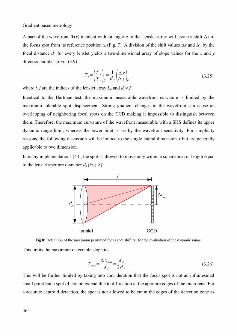
Gradient based metrology

A part of the wavefront W(x) incident with an angle α to the lenslet array will create a shift Δx of

the focus spot from its reference position xr (Fig. 7). A division of the shift values Δx and Δy by the

focal distance df for every lenslet yields a two-dimensional array of slope values for the x and y

direction similar to Eq. (3.9)

T ij=(T X

T Y )ij

=1

d f(Δ xΔ y)ij , (3.25)

where i, j are the indices of the lenslet array Lij and df ≈ f.

Identical to the Hartman test, the maximum measurable wavefront curvature is limited by the

maximum tolerable spot displacement. Strong gradient changes in the wavefront can cause an

overlapping of neighboring focal spots on the CCD making it impossible to distinguish between

them. Therefore, the maximum curvature of the wavefront measurable with a SHS defines its upper

dynamic range limit, whereas the lower limit is set by the wavefront sensitivity. For simplicity

reasons, the following discussion will be limited to the single lateral dimension x but are generally

applicable to two dimension.

In many implementations [43], the spot is allowed to move only within a square area of length equal

to the lenslet aperture diameter dA (Fig. 8) .

Fig.8: Definition of the maximum permitted focus spot shift Δx for the evaluation of the dynamic range.

This limits the maximum detectable slope to

T max=Δ xmax

d f

=d A

2d f, (3.26)

This will be further limited by taking into consideration that the focus spot is not an infinitesimal

small point but a spot of certain extend due to diffraction at the aperture edges of the microlens. For

a accurate centroid detection, the spot is not allowed to be cut at the edges of the detection zone as

46

Gradient based metrology

illustrated in Fig. 9. Otherwise, the centroid will wander off to the center of the detection area. The

diffraction limited spot size of an ideal spherical microlens can be defined by the dimension of the

first dark ring of the characteristic diffraction pattern, whose diameter is given by

d D=1.222 f λ

d A(3.27)

where λ is the wavelength of light.

An additional quality factor 1 < c < 3 can be introduced to define the deviation of a real spot from

an ideal spot, which yields for the spot size

d S=c⋅d D . (3.28)

The topic diffraction pattern will be discussed in more detail in chapter 7.1. With df = f and

including the radius of the spot, Eq. 3.26 can be extended to

T max=d A−(d S/ 2)

2 f=

d A

2 f−

1.22 c λd A

. (3.29)

Fig.9: Illustrating different definitions of the maximum permitted spot shift Δx a) with and b) without taking the

actual spot size dS into consideration.

The dynamic range could be extended if the spot movement is not limited to the area behind the

lenslet. In this case, the limitation is defined by the condition that spot of a lenslet is not allowed to

move past a spot from another lenslet. Therefore, it depends on the difference in shift Δxi+1 – Δxi of

two neighboring lenslets Li+1,j and Lij. With the slope T as the first derivative of the wavefront W

W ' ( x)=ΔWd A

=T (x )=Δ x

f , (3.30)

we can relate the dynamic range directly to the local curvature κ (x) as the second derivative

47

Gradient based metrology

κ ( x)=W ' ' ( x)=1

d A

ΔW i+1−ΔW i

d A

=1

d A

Δ x i+1−Δ x i

f, (3.31)

where we have

(Δ x i+1+d A)−Δ x i>d S (3.32)

for the condition to prevent overlapping focus points as can be seen from the dimensions in Fig. 10.

Fig.10: Illustration of the maximum permitted difference in focus spot shift between two neighboring lenslets.

This can be rearranged to (Δ x i+1−Δ x i)>d S−d A (3.33)

or using Eqs. (3.27) and (3.28), reformulated as

(Δ x i−Δ x i+1)<d A−d S ,

(Δ x i−Δ x i+1)<d A−2.44c f λd A

(3.34)

to give an indicator for the dynamic range with respect to change in focus spot shift between two

neighboring lenslets. A division by f delivers the condition for the detectable slope difference

T i(x )−T i+1(x )<d A−d S

f,

T i(x )−T i+1( x)<d A

f−2.44

c λd A

.(3.35)

Another division by dA or inserting Eq. (3.33) into Eq. (3.31) yields the maximum detectable local

curvature as

W ' ' (x )=T i(x )−T i+1( x)

d A

<1f−2.44

c λd A

2 . (3.36)

48

Gradient based metrology

Here, the focal length is considered as to be the dominating factor influencing the dynamic range

[44].As a numerical example, for an array with lenslets of diameter dA = 150 µm and f = 5000 µm at

wavelength λ = 0.5 µm, the focus spot diameter with c = 1.5 will result in dS = 61 µm.

In case of an implementation as illustrated in Fig. 8 and described by Eq. (3.29), the dynamic range

is given as the maximum detectable slope

T max=0.01195 (3.37)

which is equivalent to a maximum angle αmax = arctan(Tmax) · 180°/π = 0.685°.

For an implementation as illustrated in Fig. 10, the detectable change in focus shift is limited by

(Δ x i−Δ x i+1)< 89µm . (3.38)

A division by f·dA yields as condition for the detectable local wavefront curvature

κ ( x)=W ' ' ( x)<1.2⋅10−4 µm−1 , (3.39)

which is equivalent to a local wavefront radius of R(x) = 1/κ(x) = 8.333 mm.

These examples demonstrate that strong wavefront slopes cannot be detected by means of a SHS.

Typically, wavefront are tested after subtraction of a base reference sphere. Still, the method stays

limited to weak local wavefront curvatures.

3.5 Experimental ray tracing

Experimental ray tracing (ERT) is an optical measurement method, once introduced by Häusler and

Schneider [45] as a modification of the traditional Hartmann test, which is suitable to determine the

performance of optical components and other reflecting or transmitting objects. Recent

developments performed by Ceyhan et. al. [46][47] showed the capability of ERT to be used for the

complete quality inspection of aspherical lenses including the retrieval of the aspherical surface

shape from ray trace data, which will be further discussed in section 5.2.4.

Fig.11: Principle setup of the experimental ray tracer for transmission testing of lenses.

49

Gradient based metrology

The basic principle of ERT is based on scanning the aperture of a device under test with a test beam

and detect its change in direction after passing the device. The principle can be applied in reflection

and transmission, while for the later case, the device under test must be transmissive for the

frequency of the light. Fig.11 shows the configuration for testing aspherical lenses in transmission.

The source of the ray is usually a monochromatic laser beam whose diameter sets the minimum

lateral resolution. The correct knowledge about the initial positions (x, y) and direction of the test

beam is essential for the later analysis. The device under test is scanned with a well defined grid.

The ray will have an initial propagation direction parallel to the z-axis which coincidences with the

optical axis of the device under test. The direction of the i-th ray after passing the test object is

obtained by detecting its intensity distribution at not less than two different intersection planes

z1,...,zk along the z-axis by an conventional image sensor. The coordinates of the intersect positions

are retrieved from the captured images as centroids Ski by centre of mass calculations. In contrast to

the other gradient techniques above, the rays are traced individually. The detected slope of each

outgoing ray can be related to a certain ray incident on the aperture of the device under test.

Compared to the aforementioned Hartman test or SHS, the individual rays are allowed to cross each

other freely between the two detection planes and can make use of the complete detection area. The

maximum detectable slope

T max=d A−(d S/ 2)

2Δ z=

d A

2Δ z−

1.22 c f λd LΔ z

. (3.40)

is only limited by the detector size dA, the distance between the two detection planes Δz and the spot

size dS, as given by Eqs. (3.27) and (3.28). Compared to the case described by Eq. (3.29), Δz is not

bound to be equal to the focal length and the spot size is depending on the aperture diameter dL of

the lens under test. The quality factor c can be chosen to adapt for a change in spot size with

distance of the individual z-planes to the focal plane. The dynamic range is clearly dominated by

the distance between the detection planes, which could be chosen arbitrarily small. However, as will

be shown later, decreasing Δz will lead to an increase in uncertainty associated to the detected ray

slope. The dynamic range can as well be increased by a larger detection area.

For a lens with an f-number of f/# = f/dL = 1, the spot radius in the focal plane will be approximately

dS/2 = 0.915 µm at a wavelength λ = 0.5 µm with c = 1.5. For a typical sensor area of dA = 10000

µm and Δz = 1000 µm, a maximum detectable slope of Tmax = 4.995 can be achieved, which is

equivalent to a maximum angle αmax = 78.68°. This is a factor of 417 compared to the achievable

slope for the SHS given in Eq. (3.37), which demonstrates the enormous dynamic range available in

50

Gradient based metrology

experimental ray tracing. This allows for the detection of strongly curved wavefront without any

additional subtraction of reference spheres and enables measurement and analysis methods

impossible to be performed with the other gradient techniques. One of those methods is the direct

detection of the focal length for strong lenses with small f-numbers as will be discussed in

chapter 6.

For the determination of the ray slopes using experimental ray tracing according to Eq. (3.1), the

associated uncertainty can be found according to the law of propagation of uncertainty to be defined

as [69]

u t=[2(∣ 1Δ z∣

2

uc2+∣ TΔ z∣

2

uz2+2∣ T

(Δ z )2∣2

uc , z)]−2

. (3.41)

The uncertainty in the centroid detection uc depends mostly on system stability, signal-to-noise ratio

and discretization effects. An average value of uc = 80 nm was found by experiment over 1000

individual measurements. The uncertainty with respect to the z position uz depends on the quality of

the positioning system. The correlation between the z-axis movement and the determined centroid

coordinate on a particular z-position is described by the mutual uncertainty uc,z = ρc,zucuz, where ρc,z

is the correlation coefficient taking a value of +1 for positive T and –1 for negative T. The

uncertainty is not constant for all slopes. With larger slopes the uncertainty increases exponentially.

It is clear from the denominators in Eq. (3.41) that larger distances between the sensor positions Δz

will significantly decrease uT. Since this distance can be chosen freely within certain limits for an

ERT measurement, the resulting uncertainty can be controlled as well.

51

The Gaussian reference sphere

4. The Gaussian reference sphere

4.1 First-order optics

In 1841, Carl Friedrich Gauss expressed optical imaging by a power series expansion of the

characteristic function, where the first order represents ideal imaging describing position and image

size whereas higher orders are related to imaging errors, denoted as aberrations [48]. The series

expansion defines the intersection point of a ray with the image plane h' as a function of the ray in

the object plane h and the position of the ray in the aperture of the optical system y. In case of a

rotational symmetry in the system, the expansion will consist of odd powers only [49]. Gauss

demonstrated that for rays that obey the paraxial approximation, a lens of arbitrary complexity can

be characterized by a collection of cardinal points consisting of two principle points H, H' and two

focal points P, P', where the distances HP and H ' P ' are identified with the focal length f of the

lens [48]. The paraxial approximation represents the limiting case, where the distance and the

angles of the rays with respect to a common axis of rotational symmetry in an optical system,

commonly referred to as the optical axis, or the surface normal of a refracting surface are very

small. Using Taylor series expansion the trigonometric functions can be expanded as

cosα=1−α2

2!+α

2

4 !−α

2

6!+... ,

sinα=α−α3

3 !+α

5

5!−α

7

7!+... .

(4.1)

For small angles α, one can apply first-order approximation which will result in cosα = 1, sinα = α

and tanα = sinα/cosα = α. The rays that fulfill this requirement are known as paraxial rays. In this

case, the law of refraction takes a simple form.[50]

The radial distance in very close proximity of the optical axis is denoted as the paraxial region. As

Kingslake [51] pointed out, the paraxial approximation deals first and foremost as a mathematical

instrument to describe ideal imaging. Though the position of the Gaussian image plane si is clearly

defined and may be calculated in case of a thin lens from the object distance so and the focal length

f by

si=so f

so− f. (4.2)

52

The Gaussian reference sphere

Actually limiting the rays incident to a real optical system to the paraxial region by a small aperture

will lead to a depth of focus so immense, that no definite image could be located.

Gaussian optics is regarded as ideal with respect to imaging in that all rays diverging from an object

point are perfectly converging into an image point after propagation through a system of arbitrary

complexity. Hence, Gaussian landmarks, as the Gaussian image point, are references from where to

measure departure from perfection. [49] Optical systems are commonly optimized to fulfill its

conditions as best as possible. In its simplicity, Gaussian optics does not make a distinction between

a spherical and an aspherical surface. In case of an aspheric surface, Gaussian imaging is performed

with respect to its vertex radius of curvature [50].

4.2 Parabolic approximation of the sphere

Fig.12: Derivation of the sagittal representation for a spherical surface.

The usual symmetry of surfaces in optical systems around a common optical axis lends itself to the

application of cylindrical coordinates. Describing the shape with respect to its axial tangent plane

z = f(ρ,φ) leads to a sagittal representation, which is referred to as the sag, where the surface's vertex

is found to be at z(0,0) = 0 and z being the displacement of the surface from the vertex. Further

defining the surface to be rotational-symmetric simplifies the description by being independent of

the polar angle φ with only a dependence on the radial distance ρ left, which is related to the

Cartesian coordinates x and y over

=x2 y2 . (4.3)

The sagittal representation for a spherical surface of radius R can be obtained using the Pythagorean

theorem as illustrated in Fig. 12 which yields

z sph(ρ)=R−√R2−ρ2 . (4.4)

Using the curvature C = 1/R to prevent Eq. (4.4) from being indeterminate for plane surfaces with

R = ∞, one obtains

53

The Gaussian reference sphere

z sph(ρ)C ρ

2

1+√1−c2ρ

2 , (4.5)

known as spherometer formula. A rotational-symmetric surface described in Cartesian coordinates

can be expanded by binomial expansion as

z ( x , y)=c2( x2+ y2

)+c4( x2+ y2

)2+c6(x

2+ y2

)3+...c2n( x2

+ y2)

n , (4.6)

where in case of a spherical surface the first three coefficients are given by [43]

c2=1

2R, c4=

18R

, c6=1

16R. (4.7)

Using Eq. (4.3) to express the expansion in cylindrical coordinates results in

z sph(ρ)≈ρ

2(ρ

R )+ρ

8(ρ

R )3

+ρ

16 (ρ

R )5

+... . (4.8)

The first term of the expansion is parabolic

z par(ρ)=ρ

2

2 Ror z par( x , y)=

x2+ y2

2 R2 , (4.9)

which means any sphere may be approximated by a parabola for ρ/R << 1, which fits to the

condition of paraxial approximation. Outside of the paraxial region, zsph(ρ) > zpar(ρ) , which means

that the sag of a parabola is always smaller than the sag of the corresponding sphere. Fig. 13 shows

the percent error δz = (zpar – zsph )/zsph ∙ 100 of the approximation [51].

Fig.13: Sag error between spherical and parabolic surfaces according to Kingslake[51].

54

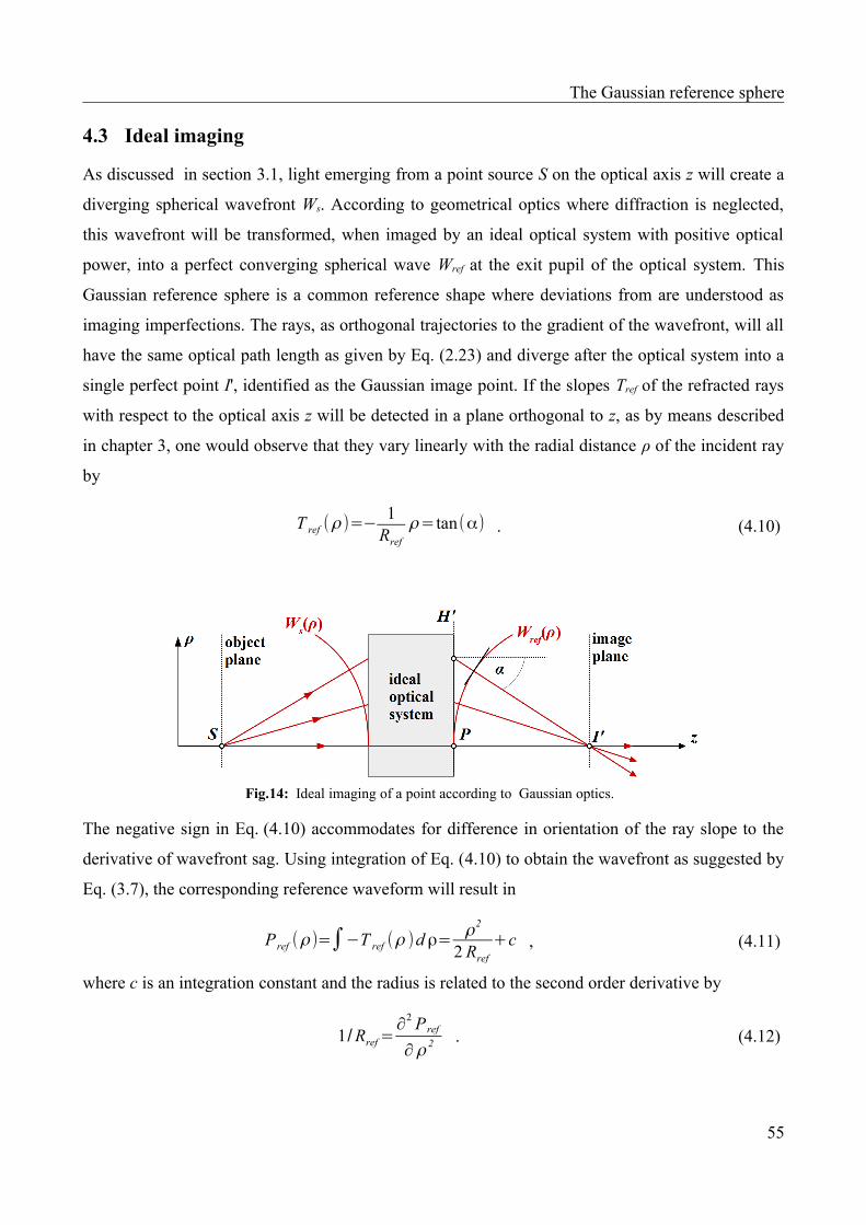
The Gaussian reference sphere

4.3 Ideal imaging

As discussed in section 3.1, light emerging from a point source S on the optical axis z will create a

diverging spherical wavefront Ws. According to geometrical optics where diffraction is neglected,

this wavefront will be transformed, when imaged by an ideal optical system with positive optical

power, into a perfect converging spherical wave Wref at the exit pupil of the optical system. This

Gaussian reference sphere is a common reference shape where deviations from are understood as

imaging imperfections. The rays, as orthogonal trajectories to the gradient of the wavefront, will all

have the same optical path length as given by Eq. (2.23) and diverge after the optical system into a

single perfect point I', identified as the Gaussian image point. If the slopes Tref of the refracted rays

with respect to the optical axis z will be detected in a plane orthogonal to z, as by means described

in chapter 3, one would observe that they vary linearly with the radial distance ρ of the incident ray

by

T ref (ρ )=−1

Rref

ρ= tan(α) . (4.10)

Fig.14: Ideal imaging of a point according to Gaussian optics.

The negative sign in Eq. (4.10) accommodates for difference in orientation of the ray slope to the

derivative of wavefront sag. Using integration of Eq. (4.10) to obtain the wavefront as suggested by

Eq. (3.7), the corresponding reference waveform will result in

P ref (ρ )=∫−T ref (ρ )d ρ=ρ2

2 Rref

+c , (4.11)

where c is an integration constant and the radius is related to the second order derivative by

1/Rref=∂

2 P ref

∂ρ 2 . (4.12)

55

The Gaussian reference sphere

The fact that Pref is of parabolic shape instead of a sphere as mentioned above indicates that

Eq. (4.11) does not represent the reference wavefront at radial distance ρ without further

approximation.

The connection between the local slopes of a curved wavefront and the detection position in a flat

plane will not create a surface of the wave where all surface points have the same optical distance to

the source and therefore, the same phase. Fig. 15 illustrates the effect. A slope value of a wavefront

W at point A will be detected in the plane D at ρD but actually has a lateral height on the wavefront

of ρA. Furthermore, the slope detected at ρD actually belongs to a wavefront V whose phase

advances the phase of the wavefront W. As a result, any technique which senses curved wavefronts

with respect to a flat detection plane will only detect a distorted form of the wavefront W unless it is

perfectly flat and therefore, fitting the shape of the detector plane. Classically, the identification of

the parabola with the wavefront is justified for rays that fulfill the condition of paraxial

approximation with α → 0 or wavefronts W(ρ) detected over an area of ρ << Rref and with W

sufficiently small [53], [54]. In these cases, the difference between the sphere and the flat detection

plane vanishes and the sphere can be approximated in first-order by a parabola as described in

section 4.2.

Practically, this problem may be minimized by using a null-setup where the wavefront is detected

with respect to a reference sphere that is subtracted from the measurement. But the stronger the

residual deviation of the wavefront, the larger the actual error is again.

Fig.15: Detecting curved input wavefronts by a flat detection plane D will result in values from different wavefrontsdepending on the position.

4.4 Reference sphere from ray slopes

The problem discussed above can be reformulated mathematically using the definitions given in

chapter 2.1. For an homogenous medium with the refractive index n = const., the direction

s(ρ, z)|z=zD of the rays at the detection line at z = zD = const. coincide with the gradient of the eikonal

56

The Gaussian reference sphere

∇χ(ρ, zD) at that line according to Eq. (2.17). According to section 2.1.5, the components of the unit

propagation vector ek = k/k0 for a plane wave are given as

ek=(p=k x

k 0,

q=k y

k 0

, l=k z

k 0) , (4.13)

where (p² + q² + l²)1/2 = 1. For a propagating of the plane wave along z with kx = ky = 0, the

propagation vector simplifies to

ez=k z

k 0

=1n

d χd z

=1 , (4.14)

the gradient of the eikonal is given by

∇χ=d χd z

=n , (4.15)

where an integration ∫n dz yields the solution

χ (z )=n z+z 0 , (4.16)

where z0 is an arbitrarily chosen reference starting point, for example the surface of a plane emitter.

One can see that the eikonal is independent of the radial distance ρ and therefore constant along

this direction for a given z. Hence, the condition for the wavefront W(ρ) = χ(ρ, z)|z=zD = constant at

the line z = zD is fulfilled and integration over the ray slopes ∫T(ρ) dρ will yield the wavefront. For

any other type of wave, the eikonal χ(ρ, z)|z=zD ≠ constant ≠ W(ρ).

However, a wavefront W(ρ) = χ(ρ, z)|z ≠ zD = constant may be retrieved from the ray slopes under the

condition that the rays do not cross between W(ρ) and the detection line at z = zD. The following

discussion will focus on solving this problem with respect to a spherical wave, which may represent

the Gaussian reference sphere.

The optical path from an axial point S, being the divergence point of a spherical wave, to a radial

distance ρD on a detector plane D positioned at distance z = r from the source can be obtained from

trigonometric relations as seen in Fig. 15 to be

χ (ρ )=√ρ 2+r2

=r

cosα, (4.17)

in case of air as constant surrounding medium with nair ≈ 1, where r is the radius of the wavefront W

whose vertex is coinciding with the detector plane at the optical axis. The relation of this eikonal to

the slope of the ray is then given by

57

The Gaussian reference sphere

T (ρ )=ρ

r=tanα=

sinαcosα

=χ(ρ)sinα

r. (4.18)

The optical path difference between all rays in the detector plane with respect to the ray at the

optical axis is given by

Δ χ (ρ )=χ (ρ )−χ (0)=χ (ρ )−r . (4.19)

From the smaller triangle of Fig. 15, the difference between the detected radial position and the

corresponding position on the wavefront can be obtained as

ρ D−ρ A=sinαΔ χ (ρ D) , (4.20)

or

ρ D−ρ A=tanαW (ρ A)=T (ρ A)W (ρ A) . (4.21)

Setting Eq. (4.20) equal to Eq. (4.21) yields

sinαΔ χ (ρ D)=T (ρ A)W (ρ A) , (4.22)

and one can write the wavefront resulting from ray slopes and eikonal as

W (ρ A)=sinα⋅Δχ(ρ D)

T (ρ D), (4.23)

which can be simplified to

W (ρ A)=r−r cosα , (4.24a)

W (ρ A)=ρ A (1−cosα)

T (ρ D), (4.24b)

where

α=α(ρ D)=arctan [T (ρ D)] , (4.25)

for -π/2 ≤ T(ρD) ≤ π/2. The result of Eq. (4.24) describes a wavefront at certain positions ρA which

can be obtained from the corresponding detection positions by use of Eq. (4.20) yielding a position

mapping given by

ρ A=ρ D−sinα⋅Δ χ (ρ D) , (4.26)

or

ρ A=ρ D+r [sinα−T (ρ D) ] , (4.27a)

ρ A=ρ Dsin α

T (ρ D). (4.27b)

58

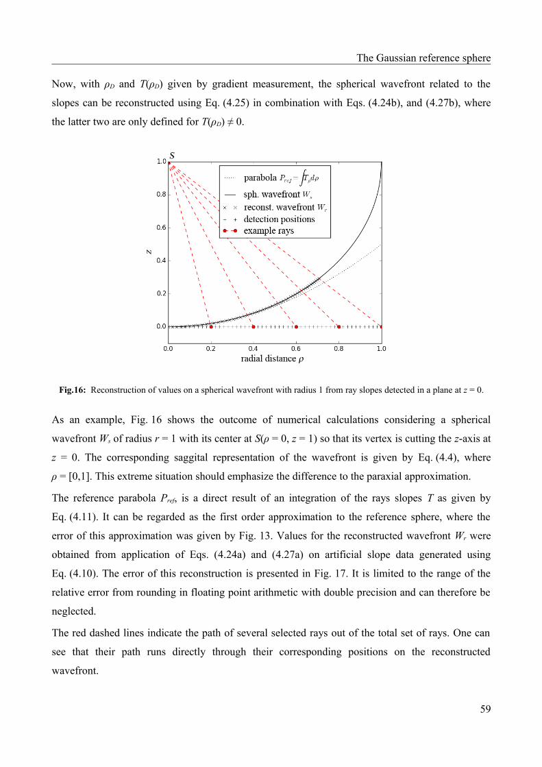
The Gaussian reference sphere

Now, with ρD and T(ρD) given by gradient measurement, the spherical wavefront related to the

slopes can be reconstructed using Eq. (4.25) in combination with Eqs. (4.24b), and (4.27b), where

the latter two are only defined for T(ρD) ≠ 0.

Fig.16: Reconstruction of values on a spherical wavefront with radius 1 from ray slopes detected in a plane at z = 0.

As an example, Fig. 16 shows the outcome of numerical calculations considering a spherical

wavefront Ws of radius r = 1 with its center at S(ρ = 0, z = 1) so that its vertex is cutting the z-axis at

z = 0. The corresponding saggital representation of the wavefront is given by Eq. (4.4), where

ρ = [0,1]. This extreme situation should emphasize the difference to the paraxial approximation.

The reference parabola Pref, is a direct result of an integration of the rays slopes T as given by

Eq. (4.11). It can be regarded as the first order approximation to the reference sphere, where the

error of this approximation was given by Fig. 13. Values for the reconstructed wavefront Wr were

obtained from application of Eqs. (4.24a) and (4.27a) on artificial slope data generated using

Eq. (4.10). The error of this reconstruction is presented in Fig. 17. It is limited to the range of the

relative error from rounding in floating point arithmetic with double precision and can therefore be

neglected.

The red dashed lines indicate the path of several selected rays out of the total set of rays. One can

see that their path runs directly through their corresponding positions on the reconstructed

wavefront.

59

The Gaussian reference sphere

Fig.17: Error in wavefront reconstruction compared to the explicit sag representation of a sphere.

The effect of the radial mapping is obvious when comparing the resulting positions of the x markers

with the original radial positions of the + markers. The approximation by integration of the slopes

only holds for the area close to the optical axis. To retrieve the location of the points on the real

wavefront, their position must be adapted with respect to W and ρ.

4.5 Aberrations

The imaging performance of spherical lenses is limited by a series of inherent characteristics,

identified with ray and wave aberrations, which are deviations from the aforementioned idealized

conditions of Gaussian optics. Rays emitted from a point in the object space will not converge to a

perfect image point after propagation through the optical system. Instead, broadening of the image

point will lead to an extended spot in the image plane or a locus of least confusion in the image

space whose center does not necessarily coincide with the Gausian image point. Though related to

imperfection, aberrations are not a result of actual flaws in the imaging system but deviations from

a highly idealized and simplified mathematical model, which is not accurate in the description of

imaging by spherical surfaces.

The most prominent aberration for spherical lenses is the spherical aberration, which is a direct

result of the spherical surface shape. In case of an ideal lens, light rays parallel to the optical axis

incident to the lens will be focused into a single perfect point P on the optical axis, denoted as the

Gaussian focal point. The condition of paraxial approximation is not fulfilled for rays that get

refracted at the edge of the lens as can be seen from the simulation example in Fig. 18. For a convex

spherical surface, the rays at the edge will intercept the optical axis prior to the Gaussian image

plane. This distance is denoted as the longitudinal ray aberration l. Furthermore, the ray will

intersect the Gaussian image plane at point P' with a transversal distance e from the Gaussian focal

60

The Gaussian reference sphere

point, designated as transversal ray aberrations. The result will be a smearing of the focal point

along the optical axis known as caustic [55].

Fig.18: Spherical ray aberrations of a convex lens.

Wavefront aberrations are defined as the difference in optical path OPD between the Gaussian

reference sphere S, with its vertex coinciding with the exit pupil plane of the optical system, and the

actual wavefront A at the same position. In this context, wave aberrations are expressed as a

function W of the exit pupil coordinates. The partial derivative of this function can be related to the

transversal ray aberrations with respect to x and y by [50]

∂W∂ x

=−ne x

R−W,

∂W∂ y

=−ne y

R−W,

(4.28)

where ex = x' – xi and ey = y' – yi , n is the refractive index of the medium behind the exit pupil and R

is the radius of the Gaussian reference sphere S. Generally, the aberration function W << R,

therefore Eq. (4.28) can be simplified to

∂W∂ x

=−e x

R,

∂W∂ y

=−e y

R.

(4.29)

where in case of air as medium, nair ≈ 1. The relations above are not limited to spherical aberrations

alone but define the general relation between ray and wave aberrations.

Identical to case of wavefront reconstruction described in section 3.2, the partial derivatives of the

wavefront function can be expanded by the partial derivatives of the orthogonal Zernike

61

The Gaussian reference sphere

polynomials. In this case, however, they will not only provide means for modal integration. The

individual elements Znm of the polynomial set can be identified with certain types of aberrations. As

an example, table 4.1 list the first 13 unnormalized elements and their physical identities.

n m Z(ρ, θ) Aberration

0 0 1 Piston

1 -1 ρ sinθ Tilt x

1 1 ρ cosθ Tilt y

2 0 2ρ2 – 1 defocus

2 -2 ρ2 sin(2θ) Prim. Astimgmatism 45°

2 2 ρ2 cos(2θ) Prim. Astigmatism 90°

3 -1 (3ρ3 – 2ρ) sinθ Prim. Vertical Coma

3 1 (3ρ3 – 2ρ) cosθ Prim. Horizontal Coma

3 -3 ρ3 sin(3θ) Vertical Trefoil

3 3 ρ3 cos(3θ) Oblique Trefoil

4 0 6ρ4 – 6ρ2 + 1 Prim. Spherical

Table 4.1: Selection of unnormalized Zernike polynomials and their physical meaning

Therefore, the expansion coefficients represent a measure of the contribution from the individual

types of aberrations to the complete imaging error.

4.6 Radius of curvature from aberrated wavefronts

To define the Gaussian reference sphere, it is sufficient to know its radius of curvature R.

Using the process described in section 3.2, it is possible to obtain the wavefront function from ray

slopes after modal integration. As was shown in section 4.3, the Gaussian reference sphere will

become a paraboloid when the slopes were to be detected by a flat plane, which is the common

situation. For the ideal imaging case, all coefficients of the Zernike polynomials vanish with

exception of the field curvature term Z02, and the paraboloid may be approximated by

P ref≈W curv=c2,0 Z 20(ρ )=c2,0⋅√3[2( ρr0 )

2

−1] , (4.30)

where r0 is the radius of the real circular aperture over which the Zernike fit is performed. On can

see that this term is dominated by a parabolic component. Its second order derivative yields for the

radius of curvature

62

The Gaussian reference sphere

Rref≈r0

2

4√3 c2,0

. (4.31)

In the presence of aberrations, the field curvature term of the Zernike polynomials alone does not

suffice to fully describe the reference parabola. Aberrations in the detected waveform will result in

additional contributions from other terms. In an orthogonalization procedure for polynomials, as the

Gram-Schmidt process described in section 2.2.2, higher orders are made orthogonal to lower ones

by subtracting components of each lower term that are not orthogonal. In case of the Zernike

polynomials, this leads to a situation in which parabolic terms will not only be found in the field

curvature terms but in higher orders as well, e. g. spherical aberrations of various orders. Therefore,

all terms that include a parabolic contribution must be regarded. Assuming a probable contribution

from all terms, the radius of curvature of the reference wavefront, equivalent to the effective focal

length, is expanded using Zernike polynomials by

Rref (0)=r 02[∑m, n

cm, n

∂2 Z n

m(0,θ )

∂ ρ 2 ]−1

. (4.32)

Notice that the radius of curvature in case of spherical aberrations becomes a function of radial

distance in case of rotational symmetry and is not constant anymore. Hence, it must be determined

at the optical axis. Due to the second order derivative, all parabolic parts will contribute as a

constant value while lower orders are sorted out by differentiation and higher orders become zero at

ρ = 0. For the evaluation of Eq. (4.32), only the radial polynomials of the Zernike with an azimuthal

degree of m = 0 are to be considered as the azimuthal part is as well sorted out by differentiation

over ρ. This results in a simplified definition of the polynomials of interest based on their definition

from Eq. (2.114)

Rn0(ρ )=∑

k=0

n /2(−1)k (n/2−k ) !

k ! (n /2−k )!(n /2−k ) !ρ n−2k . (4.33)

To further isolate the parabolic parts where ρn-2k = ρ2, we set k = n/2 –1 and obtain

Rn0(ρ)=

(−1)n /2−1(n/2+1)!

(n /2−1)!ρ 2

. (4.34)

From these, only the terms with an even radial order 2n contain a parabolic part and will be

considered, where their second order derivatives result in

An=∂ R2n

0(ρ )

∂ ρ=2

(−1)n−1(n+1)!

(n−1) !. (4.35)

63

The Gaussian reference sphere

With (n + 1)! / (n – 1)! = n (n + 1), this can be further simplified to

An=−2(−1)n n(n+1) , (4.36)

which combined with Eq. (4.32) yields for the radius of curvature

Rref≈r 02[∑n=1

∞

c2n ,0√2n+1⋅An]−1

, (4.37)

where the root is a result of the normalization constant Nnm of the Zernike polynomials defined in

Eq. (2.113), for m = 0 and only even orders 2n. For n = {1, 2, …, 6} the factor defined by Eq. (4.36)

yields {4, –12, 24, –40, 60, –84}. Therefore, the expression in Eq. (4.31) represents the first term of

this infinite series. In a practical situation, the evaluation of Eq. (4.37) can be stopped after a limited

number of terms since the contributions of the individual terms diminish significantly with higher

orders.

If the radius described by Eq. (4.37) was to be detected from a wavefront tangent to the posterior

principle plane of an optical system for the case of an incident plane wave orthogonal to the optical

axis, its value may be identified with the focal length of the optical system. However, finding the

exact position of the principle plane is difficult to execute. Here, the slopes offer a special

advantage. Since the slope of the ray in homogenous media remains the same after the device under

test, the position of its detection along the optical axis is uncritical as long as it can be related to its

incident position on the device under test. This is weakly true for the Hartmann test but especially

true for the experimental ray tracing which sets it apart from Shack-Hartman sensors where this

relation cannot be made. As an example, numerical ray tracing was used to generate artificial ray

slope data of a strong spherical lens shown in Fig. 18 with a clear aperture of 25 mm and a design

focal length of fD = 25.16149 mm at a wavelength of 632.5 nm.

n R δR

1 20.97 mm 16.66 %

2 26.56 mm 5.55 %

3 24.81 mm 1.38 %

4 25.38 mm 0.85 %

Table 4.2: Radius of curvature of the reference sphere from radial terms of the Zernike polynomials with increasing

even radial degree n

The focal length can be identified with the radius of curvature of the Gaussian reference sphere at

the exit pupil. Modal integration was performed using 46 terms of Zernike polynomials and the

radius of curvature was obtained using Eq. (4.37) for increasing n. Table 4.2 summarizes the

64

The Gaussian reference sphere

resulting value of the approximate radius of curvature and the absolute percent error δR with respect

to the expected value based on the design.Aside from the purely rotational symmetric Zernike

terms, further parabolic contributions are found for azimuthal degrees of m = 2, –2 which comprises

astigmatism of various orders, as a result to cylindrical power in the lens. If any influence of this

kind was mend to be regarded as well, further terms must be considered. The radial polynomials for

the crucial contributions that contain astigmatism are given by

Rn2(ρ )= ∑

k=0

(n−2 )/2(−1)k (n−k )!

k ! ((n+2)/ 2−k ) !((n−2)/ 2−k )!ρ n−2k . (4.38)

Setting k = n/2 –1 results in

Rn2(ρ )=

(−1)n /2−1(n /2+1) !

(n /2−1)! ((n+2) /2−n/2−1)! ((n−2)/2−n /2−1)!ρ 2

, (4.39)

and can be simplified to

Rn2(ρ)=

(−1)n /2−1(n/2+1)!

2 (n /2−1)!ρ 2

. (4.40)

Limiting to even orders n = 2 only yields

R2n2(ρ)=

(−1)n−1(n+1)!

2(n−1)!ρ 2

, (4.41)

whose second derivative concludes to

Bn=∂ R2n

0(ρ )

∂ ρ=(−1)n−1

(n+1)!(n−1) !

=−(−1)n n (n+1) . (4.42)

From this it is clear that An = 2 Bn.

Astigmatic terms of the same azimuthal degree can be combined using the identity

a cosα+b sinα=√a2+b2 cos(α−tan−1(b /a)) . (4.43)

Neglecting angular parts, the magnitude of interest is given by the square root above [54].

Therefore, the radius of curvature based on all parabolic contributions yields

Rref≈r 02[∑n=1

∞

√2 n+1 An c2n ,0⋅+√4 n+2 Bn√c2 n ,22+c2 n ,−2

2 ]−1

. (4.44)

65

Aspherical surfaces

5. Aspherical surfaces

With the advent of photography, the requirements on imaging quality of optical sytems increased

significantly and designs based on the simple first-order optics approximation made by Gauss were

not able to generate optical systems of appropriate quality. The consideration of higher order optics

including aberrations enabled systems that could approach the ideal imaging conditions from

Gaussian optics. For such systems, one could either combine elements with characteristics that

cancel each other out or deviate from the simple spherical surface shape, which aberrations adhere

to, leading to a group of aspherical surfaces. Still today, most components in optical systems, as

lenses and mirrors, are plane, spherical or a paraboloid, which results from the fact that other, more

complex shapes of needed precision were difficult and costly to produce. Newest advances in the

manufacturing field allows for the fabrication of asphercial and even freeform shapes with optical

precision.

5.1 Aspherical lenses

Traditionally, aberrations in optical systems are compensated by combinations of convex and

concave lenses of different materials. However, this leads to complex systems of a multitude of

lenses with an increased demand on alignment and higher costs. Another approach is to design the

interfacing surface so that all rays originating from a point source at the object plane F' will travel

the same optical path length (OPL(r) = l(r) * n(r)) to reach the paraxial focal point Fi.. Typical

results are surfaces of conic shape which are the base of aspheric lenses.[56]

Therefore, using aspheres instead of conventional spheres increases the imaging performance of the

system. They make additional components for aberration compensation redundant and therefore,

enable the fabrication of smaller, lighter and simpler optical systems at lower cost. The only

disadvantage is the increased complexity in the manufacturing process due to the unique shape of

the aspherical lens and the associated challenges for the related metrology principles.

An aspherical shape may be represented by one of various descriptions, such as Chebyshev

polynomials [57], Zernike polynomials [58] or even splines [59]. For a simple approach, a series

comparable to Eq. (4.8) could be used for a start to describe an aspherical surface. For a parabolic

shape, only the first term of the series is needed. However, if the base shape is mostly spherical and

of strong sag, which is the standard case for most aspherical lenses, the expansion must be

66

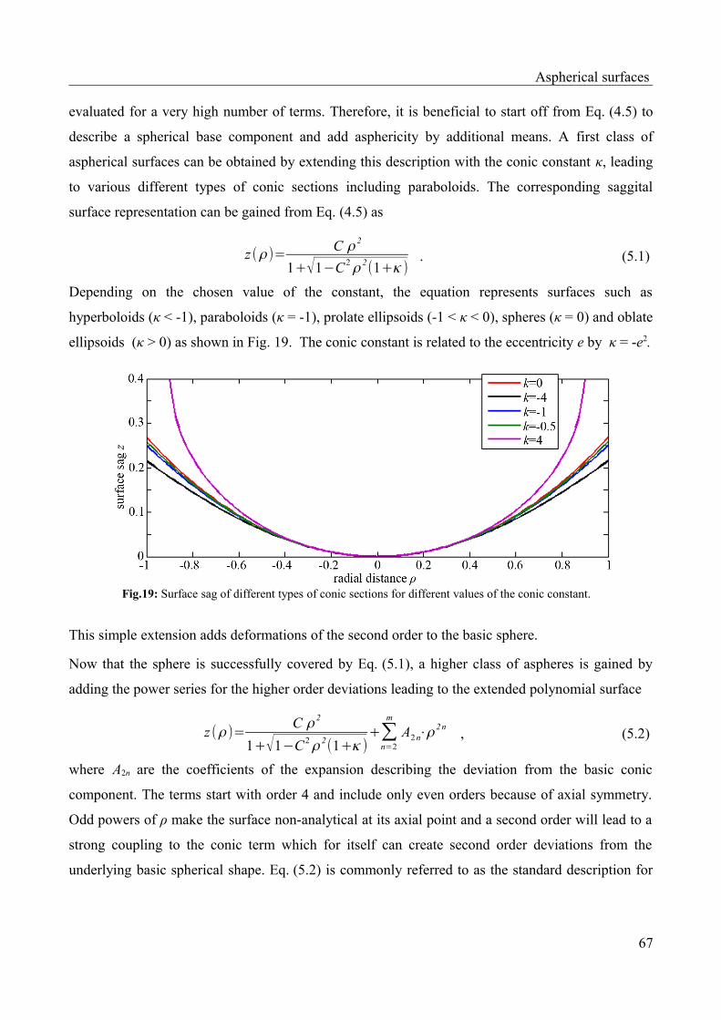
Aspherical surfaces

evaluated for a very high number of terms. Therefore, it is beneficial to start off from Eq. (4.5) to

describe a spherical base component and add asphericity by additional means. A first class of

aspherical surfaces can be obtained by extending this description with the conic constant κ, leading

to various different types of conic sections including paraboloids. The corresponding saggital

surface representation can be gained from Eq. (4.5) as

z (ρ )=C ρ 2

1+√1−C2ρ 2(1+κ )

. (5.1)

Depending on the chosen value of the constant, the equation represents surfaces such as

hyperboloids (κ < -1), paraboloids (κ = -1), prolate ellipsoids (-1 < κ < 0), spheres (κ = 0) and oblate

ellipsoids (κ > 0) as shown in Fig. 19. The conic constant is related to the eccentricity e by κ = -e2.

Fig.19: Surface sag of different types of conic sections for different values of the conic constant.

This simple extension adds deformations of the second order to the basic sphere.

Now that the sphere is successfully covered by Eq. (5.1), a higher class of aspheres is gained by

adding the power series for the higher order deviations leading to the extended polynomial surface

z (ρ )=C ρ 2

1+√1−C2ρ 2(1+κ )+∑

n=2

m

A2n⋅ρ2n

, (5.2)

where A2n are the coefficients of the expansion describing the deviation from the basic conic

component. The terms start with order 4 and include only even orders because of axial symmetry.

Odd powers of ρ make the surface non-analytical at its axial point and a second order will lead to a

strong coupling to the conic term which for itself can create second order deviations from the

underlying basic spherical shape. Eq. (5.2) is commonly referred to as the standard description for

67

Aspherical surfaces

rotationally symmetric aspherical surfaces and thus, it is covered by the standard ISO 10110-Part 12

[60] .

Fig.20: Aspherical surface described by ISO-standard description with An up to order n = 12 compared to its basic

conic component and the inherent basic spherical shape.

However, aside from not being meaningfully normalized, the polynomial expansion in Eq. (5.2) is

known to be inefficient and numerical unstable [61]. The individual terms are not orthogonal to

each other which leads to strong cancellation between terms as can be seen from Fig. 21, where

final shape is decomposed into the individual parts which are the result of each polynomial term.

Instead of approaching the shape from one direction, with increasing number of terms, the

polynomial will oscillate from addition to subtraction, negating partly the influence from lower

terms. The total number of chosen polynomials will have a profound influence on each coefficient

of the polynomial set [62].

Fig.21: Decomposition of the non-conic aspherical part (deviation from conic) into the individual parts resulting from

each term.

68

Aspherical surfaces

Furthermore, the standard polynomial becomes numerical unstable in a fitting situation at higher

orders until completely ill-conditioned for orders M > 20 [61]. When designing high quality

asphercial lenses, the surface must be optimized with high precision. Such designs result in

coefficients with a significant amount of digits. Table 5.1 shows an example design of a commercial

lens. As can be seen from the exponent, the number of significant digits increases tremendously

with the order n, easily approaching the precision limit of common computational systems which

provides a breeding ground for round-off errors.

order n 4 6 8 12 14

coefficient An 9.995e-6 -1.225e-10 7.294e-13 6.527e-21 -1.032e-25

Table 5.1: Example design values of a typical high precision apsherical lens

5.2 Metrology for aspherical surfaces

Metrology used for quality inspection of aspherical lenses in production environments focuses on

detecting manufacturing errors in the individual surfaces of the component [63]. The quality of the

lens is verified, if the deviation of the measured surface shapes from the design is within the stated

tolerances, since any deviation from the desired surface shape will directly affect the optical

properties of the lens. It is customary to decompose the global deviation ΔG = zmeas – zmeas of the

measured surface zmeas from the design zmeas into a superposition of a fitted spherical shape (best-fit-

sphere) zbfs and the residuals surface deformations ΔR. While the best-fit-sphere is sufficiently

characterized by its radius alone, the residual deformations are analyzed for relevant surface

features in the mid-spatial frequency range, which is related to the waviness in the surface

topography defined according to ISO 3274-4 [64] for features with a spatial period of

20 µm ≤ Λ ≤ 1mm. Accordingly, the geometrical form is defined for lower frequencies and the

surface roughness for the region above. Unfortunately, the definition of these boundary values is not

consistent in the literature. Aikens et. al [65] defined the mid-spatial frequency regime to be within

500 µm ≤ Λ ≤ 4 mm. Of most interest are the root-mean square (RMS) and the peak-to-valley (P-

V) values, as well as the visual appearance. Surface polishing techniques leave a characteristic

footprint in this frequency range, which can be identified from the residual deformation by a trained

eye. That is what makes deformations in this regime particularly interesting for the evaluation and

refinement of surface polishing processes and techniques.

The international standard ISO10110 [60] covers the design and tolerancing of aspherical lenses.

But there is no defined standard for the corresponding quality inspection. However, there are some

69

Aspherical surfaces

well established measurement techniques from other areas that were adapted for the surface

measurements of aspheres. An extensive round-robin test [66] on two selected aspherical lenses

involving companies as well as governmental institutes specialized in aspherical metrology from all

over Germany and abroad demonstrated that comparability of the measurement is still an issue. This

is true for comparison between different techniques and even within the same method. Techniques

as interferometry detect deviation along the surface normal of the best-fit-sphere, whereas classical

tactile systems measure the deviation along z. Furthermore, the size of the aperture over which the

lens is measured, has a significant influence on PV and even RMS of the residual deformations.

5.2.1 Interferometry

Its precision and high resolution makes interferometry the most common tool for the optical testing

of standard spherical lenses with an accuracy of a fraction of the wavelength of light. Once the lens

under test is aligned, the full aperture can be measured with a single shot, making interferometry a

parallel measurement technique. So, it was common sense to apply it as well for aspherical lenses.

But there are challenges with strong aspheres. The surface slopes of modern aspheres easily exceed

the detection range of conventional interferometers.

Interferometry is based on the superposition of a reference wavefront,

W ref ( x , y)=Eref (x , y)=Aref ( x , y)e[iΦref (x , y)]

, (5.3)

here described by its electric field component Eref with its magnitude A and the phase Φ, and a

wavefront emanating from a device under test

W test( x , y)=E test(x , y )=Atest(x , y )e[iΦtest(x , y )]

. (5.4)

Both wavefronts originate from the same spatial coherent and monochromatic light source and

interfere at a certain observation plane creating an characteristic interferogram. Deviations in the

optical path length (OPL) between both wavefronts, described as optical path difference

OPD=OPLtest−OPLref , (5.5)

will lead to constructive and destructive interference, visible as intensity maxima and minima

(fringes) in the interference pattern. The origin of the fringe pattern is a result of the superposition

of the fields

E s( x , y)=Aref ( x , y)e[ iΦref (x , y)]+Atest (x , y )e [iΦ test (x , y)] , (5.6)

which lead to a visible irradiance distribution of

70

Aspherical surfaces

I s(x , y )=E s(x , y )E s*( x , y) ,

I s(x , y )=Aref2(x , y )+Atest

2( x , y)+2 Aref ( x , y)Atest (x , y)cos [ΔΦ( x , y)] ,

(5.7)

where Es* denotes the complex conjugate of the electric field. Developing the fields further to

intensities yields

I s(x , y )= I ref ( x , y)+ I test ( x , y)⏟average intensity

+2√I ref (x , y ) I test (x , y)cos[ΔΦ( x , y)]⏟modulation

. (5.8)

and clarifies the cosine term on the right to be the origin for the fringes, where

x , y= test x , y −ref x , y , (5.9)

and is connected to the optical path difference by [67]

=2

OPD . (5.10)

Differences in the optical path relate to deviations of the test surface from the reference. Due to the

light propagating the test path two times, the deviation of the test surface from the reference ΔN will

create an optical path difference of twice its size

N=OPD /2 . (5.11)

From the modulation term in Eq. (5.3) it is evident that the pattern will show a maximum where the

optical path difference is an integer multiple of the wavelength

OPD=⋅n (5.12)

and a minimum for

OPD=⋅n1 /2 , (5.13)

where

n∈ℤ . (5.14)

In the resulting interferogram, the fringes create a contour map of the deviation of the surface under

test from a reference where the contour lines relate to a difference of ΔN = λ/2.

There are a wide variety of interferometer types for optical testing. However, the Mach-Zehnder,

the Twyman-Green and especially the Fizeau (Fig.22) are the most common configurations for the

testing of optical components. Introducing a special data collection and analysis extension, these

configurations can be made a phase-shifting interferometer. Typical references for surface testing

can either be flat or spherical ones [68].

71

Aspherical surfaces

The configuration in Fig.22 shows one possible realization for testing convex surfaces. The surface

under test is aligned so that its center of curvature coincidences with the center of curvature of the

reference sphere.

Fig.22: One possible Laser Fizeau interferometer configuration for testing convex surfaces. The computer-generated

hologram (CGH) will only be applied for test surfaces with strong deviations from a sphere.

This is a null-test configuration where a perfect match between reference and test surface will

create a fringe-free interferogram. Introducing a tilt will result in only perfect straight and parallel

fringes. The measurement results will show the normal deviation ΔN which is the deviation of the

test surface Ztest from the reference sphere Zref measured along the surface normal:

N=Z test−Z ref . (5.15)

This is in contrast to conventional surface profilers who measure the deviation along a common

direction (Δz) which is usually z. The dynamic range of an interferometer directly relates to its

capability to resolve the fringes in the observation plane when using an CCD detector. The

minimum fringe spacing must be larger than twice the pixel size and the fringe density should be

smaller than the Nyquist limit respectively [68].

The fringe density is proportional to the normal slope SN which is the rate of change of the normal

departure

S N(ρ )=d

d ρΔN (ρ ) . (5.16)

Relating the Nyquist limit to the normal slopes would result in a Nyquist slope which corresponds

to a maximum slope value of λ/4 for two neighboring pixel [61]. The fringe density can be kept low

by introducing a defocusing with moving the device under test along the z axis to compensate for

primary spherical aberrations. This will change the base radius of curvature R from the design so

72

Aspherical surfaces

that the resulting interferogram will show the residual surface deviations to a so-called best-fit

sphere zbfs(ρ) with the radius

Rbfs≠Rdesign . (5.17)

This is the origin of the aforementioned separation of the measured deviation of an aspherical

surface from its design into the radius of the best-fit sphere and the residual surface deformations.

However, strongly aberrated or aspherical lenses cannot be tested with full-aperture interferograms

by conventional interferometers due to their remarkable departure from the spherical reference

which will lead to a fringe density that surpasses the Nyquist sampling limit. One way to solve this

is to introduce an additional element to compensate for the aspherical part of the surface. Those

elements can be reflecting or refracting compensators summarized under the term null-optics as

well as real or synthetic computer-generated holograms (CGH). These null-elements are expansive

due to the precision with which they need to be fabricated. Any production errors or de-alignment

will profoundly reflect on the measurement accuracy of the system. Null-elements as the CGH are

customized for a certain design of the device under test. Therefore, CGHs are inefficient in

measurement environments with frequently changing test objects.

An alternative approach to measure strong aspherical surfaces is to divide the full aperture into

smaller segments where the fringe density is below the Nyquist limit. A subaperture stitching

interferometer divides the full aperture into several smaller circular sub-apertures which will be

stitched together to yield the full aperture. A certain overlapping and polynomial fitting are

necessary to guarantee the continuity of the sub-apertures. Another technique is the scanning Fizeau

interferometer, a standard Fizeau, where the interferogram is automatically taken at different

defocus position by displacing the device under test along the z-axis. At each position, another

annular zone is well underneath the Nyquist limit. The individual measurements are independent of

each other and therefore, no overlap is needed. But this technique is strictly bound to rotational-

symmetric surfaces. Both methods set high demands on the mechanical setup and the analysis.

Hence, all available commercial systems are very cost-intensive [68].

Due to its high sensitivity, the interferometer is extremely prone to environmental influences such

as vibrations and air turbulences. Therefore, a lot of effort is put into effective vibration isolation.

The accuracy of the system is furthermore depending on the alignment of the optical setup and the

errors being introduced by the additional optical components as relay-optics and null-elements.

73

Aspherical surfaces

5.2.2 Contact Profilers

Contact profilers, such as stylus profiler, scanning probe microscopes and coordinate measuring

machines, are scanning systems that measure single data points at a time. A tactile scanning system

relies on a probe tip such as a ruby ball or diamond tip, which is scanned over the device under test,

contacting the surface of the lens during the entire measurement process. Variations in topography

produce tip movements which may be detected by optical means and analyzed to obtain the

topography of the surface. They are a standard measurement tool for smooth surfaces of arbitrary

shape in precision mechanical engineering.

Usually, scans are performed linearly across the zenith of an asphere, or as a circular scan by

rotation of the specimen around its optical axis on an air bearing rotation stage. Tactile scanning

provides results with accuracies ranging between 0.05 to 0.3 µm depending on the inclination angle

of the asphere. Scanning a single lens takes several minutes. Furthermore, due to the direct contact

with the specimen, tactile systems have the potential to produce scratches and other surface

damages while scraping the tip over the specimen. This may be minimized by decreasing the force

of the stylus onto the surface. However, this will also increase the sensitivity for vibration and other

environmental effects on the measurement result. The ruby ball is critical for certain materials as

aluminum coated mirrors due to its chemical composition. A major problem is its wear-off over the

course of its lifetime. Since the measurement results from a convolution of the surface details with

the ruby ball, any deformation due to wear and tear reflects directly to the measurement. For these

and other reasons, manufacturer from contact profilers started to replace the stylus tip with a non-

contact optical sensor heads.

5.2.3 Non-Contact Profilers

The class of non-contact profilers comprise optical focus sensors and confocal microscopes as well

as various interferometer based sensor principles such as the Multi-Wavelength-Interferometer, the

White-Light-Interferometer and the spectral interferometer. Equivalent to the contact profilers, the

optical profilers scan the surface and determine single data points at a time. Most critical is the fact

that the light reflected from the surface under test must be captured by the relatively small aperture

of the sensors. Therefore, the movement of the sensor must follow the shape of the specimen within

a certain limit. For aspherical surface shapes, this movement sets high demands on the mechanical

setup. The information for the movement path usually originates from the design data. Errors in the

74

Aspherical surfaces

measurement will be introduced if the difference between design and specimen exceeds the

detection range [68].

5.2.4 Surface retrieval by gradient based transmission test

The surface retrieval with ERT as presented by Ceyhan [69] is focused on finding the deviation of

the real surface from the design. The design values are necessary input parameters and the deviation

is expected to be relatively small. The retrieval is based on a reverse ray tracing through the lens

under test (Fig.23) from the angle of the outgoing rays (β') to the surface of interest Z1. The

following derivations will concentrate on a ray propagating only in two dimensions for simplicity

reasons where y is the transversal coordinate and z is pointing along the initial propagation direction

of the rays.

Fig.23: Tracing a ray trough a plano-convex lens for the derivation of the relation between transmitted ray slopes and

the surface under test Z1.

A lens as device under test is made of two surfaces (Z1, Z2) that influence the propagation direction

of the ray. For the measurement the first will be the one to be retrieved. A ray parallel to the optical

axis with distance y will incident on this surface with an angle α to the surface normal at that

position which is related to the local surface slope

dZ1

dy= tanα . (5.18)

The surface will lead to a refraction of the ray which can be described by Snell's Law as

sinα n1=sinα ' n2 , (5.19)

75

Aspherical surfaces

where n2 is the refractive index of the lens, n1 is the refractive index of the surrounding medium and

α' is the angle between the surface normal and the ray inside of the lens. This angle can be replaced

by

α '=α+β , (5.20)

due to the negative relationship between α and β, leading to

sinα n1=sin(α+β )n2 (5.21)

or with the sum formula

sin( x+ y)=sin x cos y+sin y cos x , (5.22)

to

sinα n1=(sinα cos β +sinβ cosα)n2 . (5.23)

Dividing both sides by cos α leads to

tanα n1=( tanα cos β+sinβ )n2 , (5.24)

which can be rearranged to find a definition for the surface slope according to Eq. (5.18) depending

on β to be

dZ1

dy=tanα=

n2sin β

n1−n2 cos β. (5.25)

Adding the refraction at the second surface (Z2) described by

sin β n2=sinβ ' n1 , (5.26)

where

sin β=sin β 'n1

n2, (5.27)

to the definition of the surface slope gives

dZ1

dy=tanα=

n1sin β '

n1−n2 cos β. (5.28)

Rearranging the Pythagorean identity

cos β 2+sin β 2

=1 (5.29)

to

cos β=√1−sinβ 2 , (5.30)

and inserting Eq. (5.26) yields

76

Aspherical surfaces

cos β =√1−(sin β 'n1

n2)2

. (5.31)

Inserting this into Eq. (5.25) gives

dZ1

dy=tanα=

n1sin β '

n1−n2√1−(sinβ 'n1

n2)

2 , (5.32)

and replaces the unknown parameter β. Integrating over the transversal coordinate results in

Z1( y )=∫− y

y n1sin β ' ( y )

n1−n2√1−(sinβ ' ( y )n1

n2)

2dy

, (5.33)

which shows the relationship between the sag representation of the surface to be retrieved and the

angles of the outgoing rays which are the measurement outcome of the ERT. However, this is

strictly limited to lenses where the second surface is perfectly flat. In other cases, the incidence

angle of the ray at the second surface depend on the local slope at the intersection point as

illustrated in Fig.24.

Fig.24: Tracing a ray trough a double-convex lens for the derivation of the relation between transmitted ray slopes and

the surface under test Z1.

The local slope of the second surface can be defined as

dZ 2

dy2

=tanγ . (5.34)

With the refraction at the second surface described by

77

Aspherical surfaces

sin(γ−β )n2=sin (γ−β ' )n1 , (5.35)

Eq. (5.24) can be developed in a similar fashion as described in Eqs. (5.22) to (5.22)

(sinγ cos β −sinβ cosγ )n2

cosγ=(sinγ cos β '−sinβ ' cosγ )n2

cosγ,

( tanγ cos β −sin β )n2=(tanγ cos β '−sinβ ' )n1 ,tanγ (cosβ n2−cos β ' n1)=sinβ n2−sin β ' n1

(5.36)

and yields

dZ 2

dy2

=tanγ=sin β n2−sinβ ' n1

cos β n2−cos β ' n1. (5.37)

Rearranging this to

sin β=sin β ' n1+

dZ 2

dy2(cos β n2−cos β ' n1)

n2

, (5.38)

and inserting it into Eq. (5.23) to combine the first refraction with this second

dZ1

dy1

=

sin β ' n1+dZ 2

dy2(cos β n2−cos β ' n1)

n1−n2cos β, (5.39)

one obtains a relation between the angle of the outgoing ray and the local slope of the first surface

at the intersection point of the ray.

Eq.(5.20) offers the possibility to determine the first surface of aspherical shape from a lens with a

spherical second side by evaluating the angles of the outgoing rays β' which are the usual outcome

of an ERT measurement. However, it contains several more dependencies:

• the refractive index of the surrounding medium n1,

• the refractive index of the lens medium n2,

• the angle β,

• the second surface Z2 and

• the lateral coordinate y2 where the ray intersects with Z2 which is depending on the lens

thickness t.

With air as the surrounding medium, n1 can be assumed to be unity. For the lens parameters n2 and t

the usual deviation from the design can be assumed to be so small that its effect on the result is

fairly neglectable. Though spherical surfaces can be manufactured with very high accuracy, the

78

Aspherical surfaces

second surface should be characterized beforehand by an interferometer, a surface profiler or an

auto-collimator. An accurate knowledge about the second surface is mandatory for the exact

evaluation of the first surface. The unknowns left to determine are the angle β and the position y2.

This can be achieved by using an optimization process. For this purpose the complete lens has to be

modeled numerically. The model must contain a certain mathematical description of the first

surface Z1,M . Though other descriptions can be applied, it is common sense to use the customary

ISO-standard description (Eq. (5.2)) of the surface sag of a rotational-symmetric aspherical surface

shape for this purpose. Its parameters, the radius of curvature R, the conic constant κ and the

aspherical coefficients A2n of 2n-order are variables of the optimization process performed by the

least squares minimization over i rays

Q=∑i

[Z1, i−Z1, iMR , , A2n]

2=∑

i

iM

2, (5.40)

with the deviation of the actual shape (Z1,M) from the modeled (Z1) shape of the first surface

M=Z 1−Z 1

M . (5.41)

The modeled surface can be expressed using Eq. (5.20) as

dZ1M

dy1

=d (Z1−Δ

M)

dy1

=

sinβ ' M+

dZ 2

dy2M (cos β M n2−cos β ' M )

1−n2 cos β, (5.42)

where n1 from Eq. (5.20) was assumed to be 1 and Z2 must be known from prior measurement and

therefore, does not need to be modeled. The ideal minimization shall lead to the condition

limΔ

M→0(cos β −cos β M , y2− y2

M , sin β '−sin β ' M)=0 . (5.43)

For very small values of ΔM, the last unknown in the denominator of Eq. (5.20) and Eq. (5.21) may

be substituted by cosβM with the assumption that cosβ ≈ cosβM. Henceforth, the deviation from

Eq. (5.19) can be expressed by subtracting Eq. (5.21) from Eq. (5.20) which leads to

d ΔM

dy1

=dZ1

dy1

−dZ 1

M

dy1

=

sin β '−sin β 'M+

dZ 2

dy2M (cos β '−cos β ' M )

1−n2 cosβ M

, (5.44)

The retrieval method described above was tested using artificial surface data

Z1S y=Z 1

b y ; R , , A2 n

S y , (5.45)

as the sum of a base aspherical surface according to design (Z1b) and a defined periodic surface

deformation

79

Aspherical surfaces

S y =a⋅cos 2 v y . (5.46)

where a is the amplitude and v is the spatial frequency of the oscillation.

The resulting differences between the simulated and the retrieved surface were in good agreement

with standard deviations σ <1 nm for fairly low spatial frequencies. However, for higher frequencies

the deviations were found to be of significance (σ > 25 nm). The reason for the increasing deviation

was found in the limited capabilities of the model function Z1M to represent an aspherical surface

with higher frequency deformations which are strongly bound to the used number of aspherical

coefficients A2n. The higher the spatial frequency of the deformations the more coefficients are

needed. A spatial frequency of v = 1/3 lines/mm would require an order of n = 20. The usual

residual surface deformations on real lenses are expected to be in an even much higher spatial

frequency domain. The sufficient modeling of such a surface for an highly accurate retrieval, where

Eq. (5.19) could be minimized and the assumption cosβ ≈ cosβM holds, would demand a

tremendously large number of coefficients. As mentioned above, the modeled surface is described

using the standard description in Eq. (5.2). As discussed in section 5.1, this polynomial set is

inefficient since its terms are not orthogonal to each other leading to a strong cancellation between

the terms. Furthermore, they become numerically unstable for orders beyond m = 20. Therefore,

one is in a strict need for an improved polynomial representation for rotationally symmetric

aspherical surfaces.

5.2.5 Surface reconstruction from gradient deflectometric method

Instead of retrieving the surface by means of optimization based on measured gradient data from

transmitted rays, one could reconstruct the surface shape from the gradients of rays reflected from

its surface. The major challenge is the retrieval of the reflected ray by the usual limited area of the

detection device and the proper calibration of the system with its multiple local coordinate systems.

With a fixed incident direction onto the surface under test represented by the unit directional vector

s, the ray will be reflected into the direction of the unit directional vector [70]

s '=s−2n(n s) (5.47)

depending on the surface gradient z = (∂z/∂x, ∂z/∂y) = (zx, zy) at point P(x, y, z). Rearranging will

deliver the inward-pointing unit normal vector of the refracting surface

n=s−s '

2(n s ' ). (5.48)

Substituting

80

Aspherical surfaces

(n s)=√ 1−(s s ' )2

(5.49)

into Eq. (5.48) yields for the unit normal vector [71]

n=s−s '

√2 (1−(ss ' )). (5.50)

which can be related to the surface gradient by

n=[− z x

N,−

z y

N,

1N ] , (5.51)

where

N=√1+ z x2+z y

2 . (5.52)

Therefore, knowing the direction of the incident ray, the slope of the surface is encoded in the

direction of the deflected ray, which could be measured by a ray slope measurement as described in

chapter 3. Based on this, Miks and Novak [72] provided a theoretical analysis for the

reconstruction of optical smooth surfaces from a gradient deflectometric method (Fig. 25).

Fig.25: Sketch of principle and fundamental dimensions related to 3D surface topography reconstruction from a

gradient deflectometric method according to Miks and Novak [72].

In this analysis, a detection plane ξ is set at distance a from the x, y-plane of the global coordinate

system orthogonal to the z-axis. The incident ray with direction s = -z = (0, 0, -1) is piercing this

plane at point C and is reflected at point P on the surface z(x, y) under an angle of 2ε into direction

of s', where

ε=arccos(−s n)=1/N (5.53)

is the angle of the incident ray with the surface normal n at the reflection point and ε' = ε. The

reflected ray will puncture the sensor plane at point Q, which is at distance t from point C. From

81

Aspherical surfaces

Fig. 25, one can create a relation for the absolute slope of the ray with respect to the coordinate

system given by

T (x , y )= tan(2ε )=t

PC=

ta− z (x , y )

. (5.54)

Using the identity

tan (ε )=±√ z x2+z y

2 , (5.55)

in combination with Eqs. (5.51) and (5.52), the absolute ray slope can be reformulated in terms of

the surface slopes zx, zy as

T (x , y )=±2√z x

2+ z y

2

1−z x2−z y

2 . (5.56)

After rearranging and simplification, one obtains

z x2+z y

2=b±√b2

−1 , (5.57)

where b = (1+2/K2). This can be expressed as a partial differential equation

(∂ z∂ x )

2

+(∂ z∂ y )

2

=F ( x , y , z ) , (5.58)

with [72]

F ( x , y , z )=1+2T 2±

2T √1+

1T 2 . (5.59)

For a given surface model function z = f(x, y) and its partial derivatives, the solution of Eq. (5.58)

for the surface under test zi(xi, yi) may be reconstructed from measured distances ti related to surface

points Pi(xi, yi) by a non-linear least-squares minimization process described by

mincm{∑i

[M i(c0, ... , cM )=(∂ z i

∂ x i)

2

+(∂ z i

∂ y i)

2

−F (x i , y i , z i ;c0, ... , cM )]

2

} . (5.60)

The principle does not incorporate the direction of the ray slopes with respect to u and v but only

evaluates the absolute distance t. Therefore, this principle is limited to application of rotation-

symmetrical surfaces. Furthermore, knowledge of the distance a is mandatory, which can not be

known with sufficient accuracy in a real measurement situation. Solutions that also evaluate the

direction of the ray slopes are subject to current research and will be further investigated.

The parameters cm of the minimization are the coefficients of the surface model. This model must be

able to sufficiently and efficiently describe the surface under test and be at least one time

82

Aspherical surfaces

differentiable with respect to x and y. Finding a solution to Eq. (5.60) will easily fail, if the used

model is not a suitable representation of the surface under test. Numerical unstable models as the

ISO-standard equation for aspheres will further degrade the minimization process. Therefore,

similar to the situation discussed in the section before, this reconstruction will benefit as well from

an improved representation for rotationally symmetric aspherical surfaces.

The upcoming chapters will discuss several possible representations with a special focus on the

newly introduced Forbes polynomials. Their properties make them a superior solution for the

description of an aspherical surface with surface deformations.

5.3 Q-polynomials

In 2007, Forbes introduced two new representations [62] for the description of an rotational-

symmetric aspherical shape, frequently referred to as Q-polynomials, to solve the issues with

standard aspheric equation mentioned above. Instead of one single description, two sets of

polynomials were developed, each adapted for a different category of aspherical surfaces.

Depending on the degree of deviation of the asphere from the spherical shape, aspheres were

divided into mild and strong aspheres.

5.3.1 Qcon for strong aspheres

The description for the strong aspheres is a revised version of the standard definition in Eq. (5.2)

using as well a conic shape as the base component and an additional set of orthogonal polynomials

for higher order deformations. The aim was to yield a similar but more effective and meaningful

description that can basically be used to describe any kind of rotational symmetric aspherical shape,

though initially intended for strong aspheres.

Accordingly, the sag of a strong rotation-symmetrical aspherical can be represented by

z= f (ρ ; ρ max)=C ρ 2

1+√1−C2ρ 2(1+κ )⏟

base surface=conicoid

+u4∑n=0

N

ancon⋅Qn

con(u2

), (5.61)

using the normalized aperture coordinate u = ρ/ρmax, where ρmax is the maximum semi-aperture.

This set was reported to be superior to other choices when it comes to finding a best-fit with a

minimum RMS sag error to a given surface g(ρ) that can be expressed as

F (a0 , a1 , ... , am)=⟨[g (u ρ max)−u4∑m=0

M

amQmcon(u2)]

2

⟩=⟨ p(u)⟩ . (5.62)

83

Aspherical surfaces

The angled brackets represent the weighted average

⟨ p(u)⟩ :=∫A

p(u)w(u2)u du

∫A

w(u2)u du

, (5.63)

where w(u) ≥ 0 is a weight function that can be feely chosen, e.g. unity for equal weights over the

aperture. This will lead, as described in section 2.2.4, to the normal equations represented by

Eq. (2.94) with

c l=⟨g (u ρ max)u4 Qn

con⟩ , (5.64)

and the Gram matrix, whose elements are given by

Gm ,l=⟨u8Qm

con(u2

)Qncon(u2

)⟩ . (5.65)

With x = u2 the inner product from Eq. (5.65) is given by

Gmn=∫0

1

x 4Qmcon(x)Qn

con( x)dx . (5.66)

Based on this, one can derive the condition for orthogonality to be

∫0

1

x2 Qmcon( x) x2 Qn

con( x)dx=hmδ mn , (5.67)

in which case the components of the Gram matrix simplifies to Gm,m = hm with all off-diagonal

elements to zero and the normalization constants are given by

∫0

1

w(x )[Qmcon(x )]

2dx=hm . (5.68)

The condition in Eq. (5.67) defines this polynomial set to be orthogonal with respect to the surface

sag.

With the weight function w(x) = x4 = u8 and the base elements scaled to a maximum value of unity,

this condition is fulfilled if the basis is chosen to be [61],[62]

Qnconx=Pn

0,42x−1 , (5.69)

a shifted version of the classical Jacobi polynomials Pm(α, β) (x) , which in case of α = 0 and β = 4 are

orthogonal with respect to the weighting function from Eq. (2.74) w(x) = (1+x)4 and standardized

according to

Pn(α ,β )

(1)=(n+αn )=(nn)=1 , . (5.70)

84

Aspherical surfaces

Since the Jacobi are orthogonal over the interval [-1,1], Eq. (5.69) contains the shifting function

f :x ↦ 2x – 1 as an affine transformation, to map Pn(0,4) into the interval of [0,1].

Since the Zernike polynomials of n-th azimutal order are directly related to the Jacobian

polynomials by

Znm(x)=Pn

(0,m )(2x−1) , (5.71)

there exist as well a relation of the 4-th azimutal order of the Zernike polynomials to the basis [61]

Qnconx ≡Zn

4x . (5.72)

5.3.2 Qbfs for mild aspheres

As described in section 5.2.1, measuring aspheres demands the application of an null-optic due to

their strong deviation from a sphere. Forbes defined a second class of aspherical surface description

polynomials which are tailored for aspheres with a moderate deviation from a sphere, which are

simpler to produce and where no dedicated null-optic is needed. These mild aspheres can be thought

of as cost-effective aspheres. The description is specially suited to keep the fringe density in full-

aperture interferograms well underneath the Nyquist limit to be resolvable. However, their

description can be as well used for strong aspheres.

The sag of a mild rotation-symmetrical aspherical is defined by

zasph= f (ρ ;ρ max)=

ρ2

Rbfs

1+√1−ρ 2

Rbfs2

⏟base component=best fit sphere

+u2⋅(1−u2

)

√1−ρ 2

Rbfs2

⏟prefactor

∑m=0

M

ambfs⋅Qm

bfs(u2)⏟

polynomila expansion

, (5.73)

where Rbfs = radius of curvature of the best fit sphere,

Qmbfs = polynomial of order m and

ambfs = Forbes mild coefficients that describe the deviation from the best-fit sphere.

Though they have the dimension of length, the sum of coefficients do not translate directly to the

associated maximal change in sag. Instead they are a metric of the slope of the departure from the

sphere. The numerator of the prefactor in Eq. (5.73) ensures that the polynomial expansion is zero

at ρ = 0 and ρ = ρmax. In contrast to the previous descriptions, the base component is a best-fit

sphere and therefore, the polynomials describe the deviation from this sphere. The best-fit sphere is

85

Aspherical surfaces

defined as a sphere that coincides with total aspherical shape in the center where ρ = 0 and u = 0

and at the edge where ρ = ρmax and u = 1, which also implies

zbfs (0)=z asph(0) ; zbfs (ρ max)=zasph (ρ max) . (5.74)

Therefore, it is important to notice that the best-fit sphere from Eq. (5.73) is not the same as the

result of a sphere defined by Eq. (4.4) fitted to the aspherical shape. The polynomial expansion

defines the aspherical deviations from the best-fit sphere along the surface normal of the sphere,

designated as Δ in Fig.26. The denominator of the prefactor represents a conversion factor that

changes this into a deformation along the saggital direction z.

Fig.26: Sketch illustrating the difference between deviation from the best-fit sphere along the sphere's surface normal

to the saggital direction.

This can be derived from the illustration in Fig.26, in which can be seen that the deviation along the

saggital direction is Δcos θ. Using trigonometry, one obtains

cosΔ=√Rbfs

2−ρ 2

Rbfs

, (5.75)

which can be reformulated as

cosΔ=√1−ρ 2

Rbfs2 . (5.76)

The radius of the best-fit sphere can be derived from the overall aspherical shape based on the

condition given by Eq. (5.74) above in combination with the saggital representation of a spherical

surface from Eq. (4.4) resulting in

zasp(ρ max)=Rbfs−√Rbfs2−ρmax

2 , (5.77)

which can be further developed to

86

Aspherical surfaces

Rbfs− zasp(ρ max)=√Rbfs2−ρ max

2

(Rbfs− zasph(ρ max))2=Rbfs

2+ρ max

2

Rbfs2−2 Rbfs⋅zasph (ρ max)+zasph (ρ max)

2=Rbfs

2+ρ max

2

2 Rbfs⋅zasph (ρ max)−zasph (ρ max)2=ρ max

2

2 Rbfs⋅zasph (ρ max)=ρ max2+ zasph(ρ max)

2

and concludes to

Rbfs=ρ max

2+z asp(ρ max)

2

2 zasp (ρ max). (5.78)

The polynomials Qmbfs are chosen so that the associated slopes Sm (Fig.27) of the aspheric departure

from the best-fit sphere along the surface normal

Sm u=ddu

[u21−u2

Qmbfsu2

] , (5.79)

create a set of orthogonal polynomials which satisfy

⟨S m(u) Sn(u)⟩=δ mn:={0, for m≠n1, for m=n

, (5.80)

which is the inner product with the integral over the whole aperture (u = 0 to 1)

∫0

1

S m(u) Sn(u)W (u)du

∫0

1

W (u)du

=δ m n , (5.81)

where

W u=1−u2−1 /2 , (5.82)

is the non-negative weight function which is chosen to constrain the maximum slope. With

∫0

11

√1−x2dx=π/2 , (5.83)

the relation in Eq. (5.81) changes to [61]

( 2π )∫

0

1

S m(u)S n(u)W (u)du=δ mn . (5.84)

Furthermore, the polynomials are constructed so that the mean square slope of the normal departure

from a best-fit sphere weighted with Eq. (5.82) is simply the sum of the coefficients

87

Aspherical surfaces

∫0

1

[ 1r max∑m=0

M

am Sm u]2

W udu=1

r max2 ∑

m=0

M

am2 . (5.85)

This allows to constrain the maximum slope of the aspherical surface over the coefficients am

during the design phase in a simple matter, so that the fringe density in a full aperture interferogram

stays underneath the Nyquist limit [61].

Fig.27: Slope orthogonal Qbfs basis elements of order m = 0 to 5 and the associated surface slope elements.

As an example, for the first order slope we take the polynomial

Q1bfs=

1

1913−16 x , (5.86)

where x = u2 therefore

Q1bfs=

1

1913−16 u2

, (5.87)

multiply with the limit term

u21−u2

⋅Q1bfs=u2−u4

⋅13−16u2

19=

1

1913u2

−13 u4−16u4

16u6 , (5.88)

and taking the derivative with respect to u

S 1(u)=ddu( 1

√1913u2−13u4−16u4+16u6),

=1√19

26u−116u3+96u5 ,

=1√19

2 u(13−58u2+48u4

) .

(5.89)

88

Aspherical surfaces

5.3.3 Recurrence relations

To model mid-spatial frequency components of residual surface deformations as demanded in

section 5.2, the basis members of the polynomial set must be evaluated to significant high orders.

This can be achieved in a computational efficient way by exploiting the recurrence relation

connected with orthogonal polynomials. The recurrence relation for the Qcon polynomials can be

obtained from their close relation to the Jacobi polynomials as given by Eq. (5.69).

The recurrence relation with respect to n is given by [12]

a1n f n+1( x)=(a2n+x a3n) f n( x)−a4n f n−1( x) . (5.90)

For the case of Jacobian polynomials

f nx =Pn ,

x , (5.91)

the corresponding coefficients are documented in classical literature as [9]

a1n=2 n1n12n ,

a2n=2n12−

2 ,

a3n=2n2n12n2 ,a4n=2nn2n2 .

(5.92)

Fig.28: Surface orthogonal Qcon basis elements of different orders n.

89

Aspherical surfaces

The recurrence relation for the Qncon(x) polynomials can be derived from this according to Eq. (5.69)

by setting α = 0 and β = 4 and adding the factor (2x-1). The coefficients from Eq. (5.71) therefore

change to

a1n=4n1n2n5 ,a2n=−162n5 ,a3n=2n42n52 n6 ,a4n=2n n42 n4.

(5.93)

The standard form of the three term recurrence relation

f n1x =anx bn f nx −cn f n−1 x , (5.94)

can be derived from Eq. (5.90) by division with a1n

f n1x =a2n

a1n

a3n

a1n

x f nx −a4n

a1n

f n−1x , (5.95)

which yields for the coefficients of Eq. (5.94)

an=−2 n5n2

5 n10n1n2n5

,

bn=2n32 n5n1n5

,

cn=nn4n3

n1n2n5.

(5.96)

Fig. 28 shows selected orthogonal terms of x2Qmcon(x) up to order m = 50 generated from the

recurrence relation.

Similar to the Q-polynomials for strong aspheres from the previous section, the polynomial Qnbfs(x)

of order n can be derived from lower orders using a certain recurrence relation. However, in this

case the set of polynomials does not satisfy the three-term recurrence (5.13) and therefore, the

relation turned out to be an unconventional one. It was shown [74] that these polynomials are

related to a certain type of scaled Jacobi polynomials by

Pm x=am Qmbfsx bm−1Qm−1

bfsx −cm−2 Qm−2

bfsx , (5.97)

which can be rearranged to

Qmbfsx =

Pmx −bm−1Qm−1bfs

x −cm−2 Qm−2bfs

xam

(5.98)

and evaluated starting with the first two orders

90

Aspherical surfaces

Q0bfs=1,

Q1bfs=19−1/2

(13−16 x). (5.99)

The Jacobi polynomials themselves can be evaluated using the three-term recurrence relation

Pm x=2−4 x Pm−1 x−Pm−2x , (5.100)

with the initial valuesP0x =2,P1x =6−8 x . (5.101)

The coefficients an, bn, and cn can be determined starting with the constants

a0=2, a1=19

2, b0=−

12

, (5.102)

and applying for n ≥ 2 [74]

cm−2=−m m−1

2am−2

,

bm−1=−1bm−2 cm−2

am−1

,

am=[mm13−bm−12−cm−2

2 ]1 /2

.

(5.103)

This allows for the evaluation of arbitrary high orders as demonstrated in Fig.29.

Fig.29: Slope orthogonal Qbfs basis elements of different orders m.

5.4 The discrete data case

5.4.1 Introduction

Some aspects should be kept in mind when using orthogonal sets of polynomials on discrete data

sets. As mentioned before, these polynomials are only orthogonal over a clearly specified domain,

which can be recognized from the orthogonality condition, outside of which they will lose their

91

Aspherical surfaces

orthogonality. All data should be normalized to properly fit within the boundaries of the domain.

The spatial distribution of the data points should match to the shape of the domain. Though in the

analytical case a single term may suffice, a certain number of terms should be used to exploit their

orthogonality in numerical analysis.

Furthermore, as stated by Malacara and DeVore [63] as well as Mahajan [75] in case of the Zernike

polynomials, a set of orthogonal polynomials defined continuously over a certain aperture, loses its

orthogonality if used for discrete data sets, especially for lower numbers of data points N and in

case the positions of the data points are irregularly distributed. The integral in the orthogonality

condition of Eq. (5.67) clearly shows that the Q-polynomials are orthogonal for continuous surface

sag values over a radial distance between 0 and 1. Therefore, the condition is not fulfilled for a set

of discrete surface data points distributed over an approximately circular aperture. The relevance of

this problem increases for measurement techniques with low lateral resolution as Hartmann Sensors

or the experimental ray tracing in case of larger step sizes.

Hence, the polynomial set has to be orthogonalized over the sampling points of the discrete data

grid using a discrete Gram-Schmidt orthogonalization process to ensure numerical stability for

fitting with extremely high orders M, as in case of mid-spatial frequency analysis of residual surface

deviations. Furthermore, this process is necessary to justify the use of the simplified solution to

polynomial fitting described by Eqs. (2.108) and (2.109). As was shown recently by Ye et al. [76],

an analogous approach was successfully applied to the analysis of wavefront data over generally

shaped apertures using Zernike polynomials. Malacara and DeVore [63] offered a thorough

introduction to the orthogonalization process in the discrete case. A refined version of the process

was presented by Mahajan [77], which contains an additional normalization step yielding an

orthonormal set.

5.4.2 Discrete orthonormalization

Expanding a surface S by a set of bivariate polynomials Pm yields

S (x , y )=∑m=1

M

am Pm(x , y ) . (5.104)

If the surface happens to be a set SN of N data points taken at coordinates (xn,yn), the set of

polynomials Pm(xn,yn) is said to be orthogonal over this particular discrete set, if it satisfies the

discrete orthogonality condition

92

Aspherical surfaces

∑n=1

N

Pm( xn , yn)P l (xn , y n)=hmδml , (5.105)

where

hm=∑n=1

N

J n2 (5.106)

are the normalization constants, which are hm = 1 in case of an orthonormal set Hm. If a set Pm does

not fulfill this condition, which is the general case for all orthogonal polynomials defined in the

continuous sense, it can be orthogonalized using a series of either vector projection, reflection or

rotation on its elements. Analogous to section 2.2.2 with only minor differences, the Gram-Schmidt

process is an example that applies projection.

The orthogonal polynomials Jm(xn, yn) and the orthonormal polynomials Hm(xn,yn) are obtained from

the non-orthogonal basis Pm(xn, yn) by starting with J1 = P1, the m-th orthonormal and orthogonal

polynomials are given as

H m=J m

{∑n=1

N

[ J m(xn , y n)]2w( xn , yn)}

1 /2, (5.107)

where

J m=Pm−∑k=1

m−1

Dm, k H k , (5.108)

and

Dm , k=∑n=1

N

w( xn , yn)Pm( xn , yn)H k . (5.109)

The weight function w(xn,yn) can be chosen to be unity for this type of application. The newly

created orthogonal polynomials Jm and Hm differ to the original set Pm. Therefore, solving with the

new sets using Eq. (2.108) or Eq. (2.109) will yield coefficient values bm that are not connected to

the former base set. However, corresponding values for the coefficients am of the non-orthogonal set

can be retrieved from a reverse recursion given by

am=bm+ ∑l=m+1

M

bl Cm ,l , (5.110)

with aM = bM and m = 1, 2, …, M–1 using the conversion matrix

93

Aspherical surfaces

Cm ,l= ∑k=1

K=l−m

Dl , l−k C l−k ,m , (5.111)

where C1,1 = 1, m = 2, …, M and l = 1, 2, …, m–1.

Alternatively, creating a N by M matrix Pnm = P with the m = 1, … , M columns containing

n = 1, … , N evaluations of the polynomial Pm(xn, yn), one can decompose this matrix into the

factorization

P=Q⋅R , (5.112)

using a QR-decomposition, where Q is an orthogonal M by M matrix with orthonormal columns

representing the orthonormalized Hm(xn, yn) and R is a N by M upper triangular matrix, where all

elements below the main diagonal are zeros. The coefficients bm = b can be readily obtained from

b=QT⋅s , (5.113)

where s = Sn(xn, yn). To obtain the coefficient am = a related to the initial base Pm, one must solve

R⋅a=b , (5.114)

which can easily be done by back substitution with

aM=bM

RM , M(5.115)

and

am=1

Rm, m[bm− ∑

l=m+1

M

a j Rm, l] . (5.116)

This represents the matrix equivalent of what was discussed above. Some numerical algorithms to

produce the QR decomposition are based on projection by Gram-Schmidt orthonormalization or its

modified forms [78]. However, the Gram-Schmidt process is known to be inherently numerical

unstable due to round-off errors. Wilkinson reported [79] that extensive cancellations can take place

when using Eq. (5.108). A numerical stable algorithm found in popular numerical packages on

Linear Algebra is based on a series of Householder transformations, where the M columns of P are

linearly transformed by reflection about some plane to yield a vector of same length pointing into an

orthogonal base directions em. The complete matrix Q is formed explicitly as a product of

elementary Householder reflectors

Hi=I−τ vvT (5.117)

94

Aspherical surfaces

by Q = H1H2 … HM, where I is the identity matrix, τ is a scalar factor and v is a normalized vector

related to the columns of P [22]. The third alternative would be the use of a series of Givens

rotations, whose purpose is to zero out elements in R below the diagonal. The product of the Givens

rotation matrices Gi is related to the orthogonal matrix by QT = G1G2 … GM [80].

5.4.3 Numerical performance tests

Various parameters can be investigated to evaluate if the base Q-polynomials are behaving as an

orthogonal set and what difference makes the aforementioned orthogonalization or even an

orthonormalization. For the evaluation, numerical examples are considered by simulating an

aspherical surface using the polynomial expansion of Eq. (5.2) with the following coefficients

A4=4.36653e-7,A6=−2.21714e-10,A8=−1.70412e-13,A10=−3.68093e-17,A12=8.94436e-21,A14=1.85012e-23,A16=−6,27043e-27 ,

(5.118)

taken from a typical design of an high-precision aspherical lens. The surface is sampled using an

even square grid of 101x101 points and cut to a circular aperture leaving a total of N = 7845 data

points. The low sampling was chosen to emphasize the effects resulting from the difference

between polynomials orthogonal in the discrete and continuous sense.

Fig.30: Selected coefficients of order m = 3 (left) and m = 4 (right) resulting from a best-fit using matrix inversion fordifferent number of polynomials M.

In an orthogonal set of polynomials the individual terms are not influencing each other and

therefore, removing a certain term from the minimization will not affect the coefficients of any

other term, making their value independent from the total number of used terms M. Fig. 30

95

Aspherical surfaces

demonstrates the change in the coefficients of third and fourth order for different numbers of used

polynomial terms. The values are a result of a best-fit in the least-squares sense to the simulated

surface using the matrix inversion method from Eq. (2.100). The remarkable change for different

number of terms in case of the base Qcon-polynomials may be regarded as a clear indication that this

set, though orthogonal in the continuous case, is not orthogonal for this case of discrete data. At the

same time, the coefficients aortho of the orthogonal set are completely independent of the number of

coefficients, which indicates that the orthogonalization using the procedure from the last section

was successful.

Fig.31: Mean value of the individual polynomial terms of order m > 0 for the base set Qcon and its orthogonalizedcounterparts. Right hand side shows a comparison of the orthogonal terms only.

The same holds for the orthonormal polynomials though not included in the graph, since its order of

magnitude would scale the plot so that the behavior of the base polynomial cannot clearly be

observed.

Another characteristic of orthonormal polynomials is that the mean of each individual term <Qm>

should be zero for all orders m > 0. Therefore, with the first term Q1 = 1, the total mean of a surface

S expanded by these polynomial terms can be estimated by the coefficient a0. The results in Fig. 31

show that the best estimate can be obtained from the orthonormal set showing the smallest

deviations in the order of 10-17. The base polynomials on the other hand show deviations of 15

orders of magnitude larger compared to the results of the orthonormal set. For the orthogonal set,

though not as good as the orthonormal set, the deviations are still 13 orders of magnitude smaller

compared to the non-orthogonal set resulting in a sufficient estimate.

Section 2.2.4 presented two different types of solutions to the least-squares problem, the more

classical direct matrix inversion method described in Eq. (2.100) and the special simplified

solutions for orthogonal polynomials of Eqs. (2.108) and (2.109). The difference between the

96

Aspherical surfaces

coefficients resulting from both solutions is plotted in Fig. 32. While the differences for the

orthogonal and the orthonormal set are negligible, the differences for the Qcon-polynomials are in

the range of 10-100 nm. These values are within the specification range of modern high precision

aspherical surfaces. Therefore, the simple solution is not an appropriate alternative to the classical

matrix inversion method for these polynomials.

Fig.32: Difference between coefficients from simplified solution bm to coefficients from matrix inversion am. Right

hand side focuses on the results from the orthogonal terms.

However, the matrix inversion method was reported to be numerical unstable. The matrix condition

number of the associated Gram matrix and its reciprocal form from section 2.2.4 can be used as an

indicator for the numerical stability of this solution based on the used polynomials. The change of

the reciprocal condition number over the number of data points N for different types of polynomials

till order m = 16 is plotted in Fig. 33, where values near zero denote an ill-conditioned matrix.

Fig.33: Reciprocal condition number of Gram matrix.

Here, the power series expansion of Eq. (5.2) was included for comparison reasons, demonstrating

its obvious ill-condition regardless of the number of data points given. On the other hand, with a

97

Aspherical surfaces

constant value of unity, the Gram matrix for the orthonormal polynomials is always well-

conditioned independently from N. The base polynomials show a clear dependency where the

condition for N < 103 is similarly ill compared to the power series expansion. For higher values, the

condition stays close to ill with very little improvement of the situation for increasing N. This

indicates a certain potential for numerical instability using the matrix inversion method.

Surprisingly, the orthogonal polynomials are in a comparable range, indicating the same potential

tendency to numerical instability. This illustrates a further advantage of the additional normalization

step over the pure orthogonalization.

5.4.4 Modeling residual surface deformations

To evaluate the performance of the Q-polynomials for the description of mid-spatial frequencies,

artificial residual surface deformations ΔR(ρ)were designed inspired by typical results from real

aspherical lens surface as shown in Fig. 34.a. Using a simulation enables full control over the

properties of the test surface. The artificial surface data was created by

Δ R, sim(ρ )=z i(ρ )+ni , (5.119)

where the first element represents the characteristic surface waviness constructed from a linear

combination of two periodic functions of different periods with an magnitude of 100 nm

z i(ρ )=0.0001[cos(ρ )+cos (π /4 ρ )] , (5.120)

and the second element emulates the surface roughness as a noise component based on standard

normal distributed random numbers with µ = 0 and σ = 5 nm.

Fig.34: Residual surface deformations from (a) a measurement of a real aspherical lens and (b) simulation with

N = 201 sample points.

98

Aspherical surfaces

As shown by the comparison in Fig. 34, the resulting shape (right) made from this simple model

makes a good representative for residual surface deformations of high quality lenses (left). In both

cases the number of surface points were N = 201. Since the simulation involves surface data and not

surface slope data, the sag orthogonal set of Qcon-polynomials was chosen. A series of fits to the

artificial shape were performed with increasing number of terms from the polynomial set. The

series was stopped when the RMS of the fit residuals were below the given standard deviation of

the noise component, which was reached at M = 132.

Fig.35: Fit of a Qcon-polynomials up to order M = 132 (top) and the residuals of the fit (bottom) showing good

approximation of the given shape by the polynomials.

As can be seen from Fig. 35, the underlying mid-frequency shape was approximated with high

accuracy and the residuals seem to be purely random distributed. Fitting to such a high number of

terms necessary to gain this result could never be done with the standard description. The

Qcon-polynomials proved their ability to model residual surface deviation in the mid-spatial

frequency regime, which can be used to analyse measured aspherical surfaces and to improve the

99

Aspherical surfaces

precision of the surface retrieval discussed in section 5.2.4. Furthermore, expanding the high order

surface deviations with such a complete set of orthogonal polynomials opens up the possibility to

generate a characteristic surface spectrum of the aspherical deviation from the conic base, where the

resulting coefficients represent the magnitude of the individual frequency components [81].

Different lens designs could be identified by the shape of the spectrum. The challenge would be to

connect the resulting spectral distributions with physical meaning to raise its significance.

100

Focal length

6. Focal length

For any optical application, the focal length f, also known as focal distance, of a single lens or an

optical system is the most important property related to its optical performance. In case of the most

common optical component, the simple spherical lens, it is most often the only parameter of major

interest. Though it is of such practical importance, its definition and actual validity originates from

the very theoretical and idealized Gaussian optics where it is bound to the paraxial approximation,

which only allows rays with very small angles in close vicinity to the optical axis. However, in the

usual real test and application situation, this condition is not met.

After defining the essential parameters and dimensions connected to the focal length of a single

lens, this chapter will introduce three numerical methods for its determination from ray slopes based

on relations from classical Gaussian optics. The discussions about numerical stability and

sensitivity will be supported by numerical analysis using ray tracing simulations. Results from

repeated measurements of an experimental ray tracing system will provide an impression of the

achievable repeatability and an estimate for the resulting error in a real measurement situation.

6.1 Basic dimensions

Fig.36: Schematic drawing of relevant dimensions with respect to focal length and ray slopes in case of a singlespherical lens.

According to Gaussian optics, the posterior focal length f' is defined as the distance from the

intersection point P2 of the rear principle plain H2 with the optical axis z to the rear focal point F2 as

shown in Fig. 36 [82]. An alternative designation for the parameter is the effective focal length to

101

Focal length

distinguish it from the more practical back focal length fBFL which describes the distance between

the vertex of the last real surface V2 and the paraxial focal point.

6.2 Calculation of the design focal length

The effective focal length of a single spherical lens can be calculated from its design parameters

using the lens maker's formulas. According to Gaussian optics, the optical power of a spherical

refracting surface with a radius of curvature R, which separates two homogeneous media of

refracting index n0 and n1, is given by

P=n1−n0

R. (6.1)

In case of thin lenses, where the axial thickness t can be neglected, its total optical power P = 1/f is

given by the sum of the powers of the individual spherical surfaces that constitute it

P=P1+P2=n1−n0

R1

+n2−n1

R2. (6.2)

With the media at both sides of the lens being air (n0 = n2 = 1), one obtains [52]

P=1f=(n−1)[ 1

R1

−1R2 ] , (6.3)

which is a special case of the standard lens maker's formula for thick lenses

P=1f=(n−1)[ 1

R1

−1R2

+(n−1)

n1R1

1R2

t] . (6.4)

According to Goodman [83], a lens may be regarded as a thin lens if a ray leaves the lens at the

approximate same lateral coordinate at which it entered the lens on the first face. Therefore, the

lateral translation of the ray within the lens could be neglected.

For aspheres, the radius of the aspherical side R1 will gain additional power from second order

surface shapes

P=1f=(n−1)[ 1

R1

−1R2

+( (n−1) tn R1e R2)] , (6.5)

with

R1 e=R1

1+R1 2 a2, (6.6)

where a2 is the coefficient for the second order term in the ISO standard equation for aspherical

surfaces.

102

Focal length

The front focal length (FFL), representing the distance between the front focal point and the vertex

of the first surface can be calculated from the effective focal length by

FFL= f (1+(n−1)tn R2

) . (6.7)

Similarly, the back focal length (BFL), being the distance from the vertex of the last surface to the

rear focal plane [49]

BFL= f (1−(n−1)tn R1

) . (6.8)

6.3 Measurement techniques

There exist a wide variety of techniques that can be used to determine various types of focal length.

All techniques have their own advantages and disadvantages as well as limitations. Some of them

only work well for thin lenses, whereas others are especially suited for long focal lengths. High

accuracy usually involve highly sophisticated test equipment with complicated setup procedures

and low flexibility regarding different types of specimen. Often, the problem of correctly

determining the principle plane is avoided and only the back focal length is delivered. The biggest

problem arise from the accurate determination of the effective focal length in case of thick lenses

with short focal length. These strong lenses of high optical power are beyond the dynamic range of

interferometry. Traditional methods, such as the nodal slide [84], the autocollimation and the image

magnification methods as well as the Foucault knife-edge test [85] are based on the principle of

geometrical optics, offer low to moderate accuracies and are better suited for shorter focal lengths.

Moiré deflectometry [86] relate the focal length of the lens under test to the rotation angle of a

projected Moiré pattern, while Talbot interferometry [87] makes use of the periodic self-imaging

effect of coherent light in free space propagation behind a grating. In a similar manner, newly

proposed techniques using Lau phase interferometry [88], [89] make extensive use of the diffraction

grating theory and self-imaging effects to derive the focal distance from the phase map. Grating

shearing interferometry [90] determines the focal length by analyzing the diffraction pattern

generated by a phase grating positioned at the expected focal point of the lens. Based on Fourier

optics, Horner [91] showed that the focal length can as well be determined making use of the

Fourier transforming properties of a lens. The fiber optic method [92] is another novel method that

uses a bundle of fibers in an autocollimator setup. The recently introduced reference plate method

103

Focal length

[93], is a simple technique based on the dependency of the numerical aperture on the focal length,

which is derived by measuring front and back side reflections from a reference plate in a confocal

setup. Reported measurement errors of 5% makes it a suitable method where only lower accuracies

are sufficient. The error increases with smaller numerical aperture due to the axial resolution being

limited by the Rayleigh range. This basic idea could be enhanced using laser differential confocal

measurements, a technique initially applied to test lenses with ultra-long focal lengths [94]. It was

reported to measure the back focal length with an error of 0.01%. Newest developments allowed for

the measurement of lenses with shorter focal lengths [95] and simplified the initial test setup design

[96]. However, the experimental setup is complex and the technique cannot measure the effective

focal length without knowledge about the shape of the lens. In the following, two techniques are

explained in more detail which belong to the group of gradient based transmission test.

6.3.1 Simplified Hartmann-Shack method

A simple method based on the SHS was introduced by Wu et al. [97]. The lens under test is

illuminated by a collimated ray bundle of defined diameter representing an parallel incident wave.

The shape of the wavefront after passing the lens is sampled using a microlens array. The Shack-

Hartmann Sensor will return a slope value indicating the integral light direction over each micro

lens of the array

Fig.37: Schematic of relevant dimensions for the principle of the simplified Hartmann-Shack methodaccording to Wu et al.[97].

From Fig.37 on can derive

tanα 1=k+b

f s

; tanα 2=kf s

. (6.9)

Solving the later expression for k and substituting it into the former delivers

104

Focal length

tanα 1=tanα 2 f s+b

f s

=tanα 2+bf s

, (6.10)

which can be reformulated as

f s=b

tanα 1−tanα 2. (6.11)

Longitudinal aberrations will cause fn,n+1 to vary for different pairs of neighbouring microlenses mn

and mn+1. A weighting using the intensity In over the n-th microlens was proposed to calculate a

centroid from the quantity of different f by

f s=( I 1+ I 2) f 1,2+( I 1+I 3) f 1,3+...+( I n−1+I n) f n−1, n

(n−1)(I 1+ I 2+...+I n), (6.12)

Here, fs is not the focal length of a lens under test in front of the microlens array but the distance

from the microlens array to the focal point. An aperture in front of the lens can be used to adjust the

diameter 2rin of the incident collimated light so that its size on the SHS fits the entrance pupil

diameter 2rSHS of the sensor. With both values known, the focal length f can be derived from

dimensional relations by

f =f s⋅r in

rSHS, (6.13)

The use of the aperture will decrease the influence of light coming from the outer areas of the lens

where the spherical aberrations are the strongest. Nevertheless, the diameter of the aperture cannot

be chosen freely for the conditions of Eq. (6.9) to hold. Therefore, aberrations cannot be totally

minimized and f must not be compared with the effective focal length.

Fig.38: Schematic of relevant dimensions for the setup of the simplified Hartmann-Shack method according to Wu et al. [97].

105

Focal length

Experimental results of three doublet lenses performed by the authors yielded errors of around 1%.

Most critical is the correct setting of the aperture so that the light behind the lens fills exactly the

entrance pupil of the microlens array. This is not trivial to achieve and prone to errors.

6.3.2 Multi-Curvature Analysis using SHS

Neal et al. [35] determined the focal length from a series of wavefront curvature evaluations and

hence denoted it as multi-curvature analysis. As illustrated in Fig. (39), for a SHS at a fixed distance

L behind the lens under test, wavefronts with various radii R = f (Δz) with R ∈ ℝ+ are created by

shifting a point source S along the optical axis z varying the distance Δz to the front focal point F.

Each value of curvature κ(Δz), or of the wavefront radius of curvature R(Δz) = 1/κ(Δz) as its

reciprocal, is determined from a polynomial expansion to wavefront data obtained from the SHS.

Fig.39: Principle setup and dimensions for measuring the focal length of a positive lens using a SHS

according to Neal et al.[72].

The focal length is derived according to the image formation by the thin lens approximation as

1f=

1so

+1s i

=1

f +Δ z+

1R+L , (6.14)

where so is the object distance and si the image distance. Solving for the wavefront curvature yields

κ (Δ z )=1

R(Δ z )=

Δ z

f 2+Δ z ( f −L)

. (6.15)

A non-linear least squares which minimizes

F ( f , L)=∑i[κ i−κ (Δ zi ; f ,L)]

2

(6.16)

106

Focal length

can be used to obtain values for f and L from the observation data κi(Δzi). Since Δzi is unknown, it is

replaced in the definitions above by a distance zi – z0, where z0 is an arbitrarily chosen fixed

reference point on the z-axis. Setting z0 = 0, one can replace Δzi by zi.

An integral part is the expansion done to perform a modal integration as discussed in section 3.2 on

the slopes as local gradients which are given in Eq. (3.25). As further discussed in section 4.6, the

central radius of curvature of a wavefront is equivalent to the second derivative of the complete

reference sphere, which becomes a reference parabola in case of a flat detection plane for the

slopes. Neal et al. used only the defocus or field curvature part of the wavefront for their evaluation.

This part is defined by

W≈W defocus (x , y )=c2,0⋅Z 20( x , y) , (6.17)

using the defocus term of the Zernike polynomial in Cartesian coordinates

Z20( x , y)=2( x

r )2

+2( yr )

2

−1 , (6.18)

where r is the radius of a circular aperture encircling all sample positions used to normalize the

position coordinates so that √ x2+ y2

≤1 , as the Zernike polynomials are only orthogonal over the

unit circle. Going from wavefront W(x,y) to curvature κ(x,y), one has to differentiate the right side

of Eq. (6.17) and will get for its partial derivatives with respect to x and y

∂Z20

∂ x=

4r 2 x ;

∂Z 20

∂ y=

4r2 y , (6.19)

where we imply ∂Z∂ x

=T x ,∂Z∂ y

=T y , (6.20)

The radius of curvature R can be calculated according to

R=1κ=

1b=

1f ' ' ( x)

, (6.21)

where

b=f ' (x )

x, (6.22)

With

f ' ( x)=∂W defocus( x , y)

∂ x=c2,0

∂Z 20

∂ x=

4 c2,0

r 2 x , (6.23)

using (6.21) in (6.20) delivers

b=4 c2,0

r2 , (6.24)

107

Focal length

and according to (6.19) the radius of curvature concludes in

R=1b=

r 2

4 c2,0, (6.25)

as can be found in [35]. However, this holds only for the case that no aberrations are present as

discussed in section 4.6. In presence of aberrations, the defocus term will not suffice to evaluate the

total radius of curvature. As a consequence more terms must be added into this valuation.

This technique was realizes in an experimental setup and delivered focal length values for

comparison as discussed later in section 6.6.

6.4 Effective focal length from ray slopes

As discussed in section 4.6, in case of collimated incident light parallel to the optical axis z,

aberration free lenses will create a spherical wavefront W(ρ). When tangent to the principle plane,

the radius of this Gaussian sphere will be equal to the focal length of the lens and could be retrieved

from modal integration over the ray slopes using the second order derivative of the radial

component of the Zernike polynomials as long as enough terms are included. For an appropriate fit,

this may include up to 46 terms and more. This chapter will focus on other simpler methods to

retrieve the focal length from the ray slopes .

6.4.1 Fundamentals

As mentioned before and illustrated by Fig. 36, in case of collimated incident light parallel to the

optical axis z, aberration free lenses will create a spherical wavefront W(ρ), whose radius will be

equal to the focal length of the lens if its vertex is positioned at the principle plane. This is

commonly understood as the Gaussian reference sphere. In this reference case, the slope of the

outgoing rays Tref will vary linearly with radial distance ρ ∈ℝ≥0 of the incoming ray by

T ref (ρ)=−1f efl

ρ= tanα , (6.26)

which is identical to Eq. (4.10) and can be reformulated to

f efl=ρ

−T ref (ρ )=

ρ−tanα , (6.27)

a relation commonly known from popular literature dealing with Gaussian optics [42].

108

Focal length

6.4.2 Linear slope analysis (LSA)

Based on Eq. (6.26), the effective focal length could be derived from a ray slope measurement by

performing a simple linear fit of P(ρ) = c1ρ +c0 to the slope function T(ρ) where the effective focal

length concludes to

f efl≈−1 /c1 . (6.28)

However, as discussed in section 4.5, many real lenses and especially spherical lenses suffer from

various aberrations and will not produce a perfect spherical wavefront. The smaller the ratio of focal

length to the effective aperture of the lens, commonly referred to as f-number , the stronger will be

the impact of spherical aberrations. In this case, the ray slopes do not show a simple linear behavior

anymore as described by (6.26).

Fig.40: Impact of aperture size on linear fit to ray slope cross section data from ray tracing simulation of strong (N ≈ 1)lens.

As can be seen from the dotted line in Fig. 40, which represents simulated ray slope data of a

spherical lens, spherical aberrations dominate for this strong lens adding a shape of 3rd polynomial

order. To retrieve the focal length according to Eq. (6.26), linear functions were fitted to the

simulated slope data for three different diameters of the test aperture on the lens centered on its

optical axis. The best fit in a least squares sense for each case is represented by a straight line in the

plot. One observes that the results for the slope, and therefore the focal length, is not constant

anymore and changes with the used aperture size to achieve a best fit of the linear model. Higher

109

Focal length

values are found at the edges where the aberrations are the strongest. Therefore, similar to other

measurement techniques, measuring non-aberration free lenses over larger aperture areas than in the

very close vicinity of the optical axis will create values shorter than the actual effective focal length,

as can be seen in Fig. 41. The result will be focal length as a function f of the aperture a, where the

effective focal length can be found at fefl = f(0). For this to obtain, one must measure with an

infinitesimal small aperture which cannot be realized. However, this value can be closely estimated

from the available slope values.

The focal length function, as shown in the simulation example in Fig. 41, typically follows a clear

exponential trend with an expected minimum at f(0). Polynomial extrapolation can be used to

estimate a value of f at this point. For this, the shape of the function will be expanded by a

polynomial function P(a) of degree M as

f (a )≈∑m=0

M

cm P(a) , (6.29)

and the effective focal length can be extrapolated by the coefficient of the constant term

f erl≈c0 . (6.30)

P(a) can be chosen to be a simple polynomial or one of the various orthogonal polynomial

sequences.

Fig.41: Focal length depending on relative aperture size resulting from several linear fits to simulation data overdifferent aperture sizes.

110

Focal length

6.4.3 Local Curvature Analysis (LCA)

Another approach to the effective focal length can be found from the relation between the focal

length and the first derivative of the slope from Eq. (6.26) representing the curvature κ of the

reference sphere given by

f efl=1κ =−[ ∂T (ρ )

∂ ρ ]−1

. (6.31)

Similar to the focal length function, the spherical aberrations will cause the curvature to be a

function depending on the radial distance instead of a constant. Its values may be derived from

discrete slope data by computing finite differences using the symmetric difference quotient [98],

also called the central difference method

κ (ρ )=∂T (ρ )∂ρ

≈T (ρ+Δρ )−T (ρ−Δρ)

2Δρ, (6.32)

where Δρ equals the distance between two data points. This approximation to the tangent line might

be more accurate for small values of Δρ compared to the single sided estimation. However, very

small values of Δρ as well as values that cannot be represented with a limited number of digits after

the decimal point will yield large round of errors from the summation and subtraction in floating

point arithmetic due to cancellations [99], a problem similar to the numerical integration as stated in

section 3.2. This may be improved by automatic differentiation [100] or using the complex-step

derivative formula, where complex variables are used to estimate derivatives of real valued

functions [101].

Fig.42: Focal length depending on relative aperture size resulting from several linear fits to simulation data overdifferent aperture sizes.

111

Focal length

The effective focal length is obtained here by fefl ≈ 1/κ(0). Though similar in approach, this function

should not be confused with the aforementioned focal length function, as values outside of κ(0) do

not coincide or are related to any focal length values.

6.4.4 Equivalent Refracting Locus

The third approach makes use of the basic definition of the posterior focal length f ' in Gaussian

optics being the distance between the focal point F2 and the output principle point P2, in this case

with respect to a particular observation plane Z, as shown in Fig. 42. It is worth noticing that in case

of non-paraxial lenses with aberrations, the virtual surface created by points of intersection of

incident and refracted rays are not a flat plane but will result in a rotational symmetric curved shape

denoted by Kingslake [51] as the equivalent refracting locus ERL. In the paraxial region close to the

optical axis, the locus will resemble the principle plane H'. In a similar manner, the longitudinal ray

aberrations L will cause the position of the focal point to be a function of the radial distance.

Knowing the intersection height rρ of a certain ray incident at radial distance ρ with the observation

plane Z and the angle αρ of the ray with the optical axis z, the corresponding distance to the focal

plane is given by

z FOC (ρ )−r ρ

tanαρ

, (6.33)

and similarly, the distance to the principle plane is given by

z ERL(ρ )ρ−r ρtanαρ

, (6.34)

using trigonometric relations. Independent of the point of observation, the focal length concludes to

be the difference

f ' (ρ )=z FOC (ρ )− zERL(ρ )=−ρ

tanαρ

=−ρ

T (ρ ) , (6.35)

which is a reformulation of the relation from the classical Gaussian optics in Eq. (6.26). Here,

including the influence of spherical aberrations leads to a dependency of the focal length on the

radial distance.

Analogous to the previous approaches, the effective focal length can be found at fefl = f '(0).

However, for the limit case of paraxial optics with ρ → 0 the angle αρ will diminish whereby the

denominators in Eqs. (6.33) to (6.35) will approach zero and the relations become undefined. The

value for the effective focal length can be interpolated from values evaluated at ρ ≠ 0 by expanding

112

Focal length

Eq. (6.35) by a polynomial sequence as described by Eqs. (6.29) and (6.30). This approach will be

denoted henceforth as the classical Gaussian relation (CGR).

6.4.5 Reflective surfaces

Aside from lenses, mirrors are the most common used optical elements for focusing and imaging

applications. In lenses, the light is redirected by refraction at minimum two successive surfaces

representing the interface between two materials with different refractive index n. Whereas in

mirrors, the light is deflected by a reflection on a single specular surface. As a result, the

wavelength dependency of n leading to chromatic aberrations is avoided in case of mirrors.

Furthermore, they can be used to fold long optical propagation lengths to fit into limited space. For

radiation with wavelength from certain regions of the electromagnetic spectrum like IR and UV,

mirrors are the favored optical element, if one wants to avoid the high absorption losses inside of

available optical materials [104]. Similar to lenses, a mirror possesses an optical power in case of

surface curvatures κ ≠ 0. For a spherical concave mirror with a radius of curvature R, the principle

focal length is given by f = R/2. Compared to lenses, the principle point P and the surface vertex V

coincide (Fig.43). Hence, there is no difference between the theoretical focal length and any

mechanical relevant distance. The mirror surface is equal to the equivalent reflective locus from

section 6.4.4.

Fig.43: Sketch of principle and fundamental dimensions with respect to focal length determination from ray slopes incase of reflective surfaces.

113

Focal length

The methodology for the determination of the effective focal length described above can be applied

here as well without further revaluation. The major difference is the change in propagation direction

from z to -z. The reflected rays represent the surface normals of the emitted wavefront W(ρ). The

surface normal of the mirror represent the half angle between incident and outgoing ray. For the

reference case of Gaussian optics, a wavefront with its vertex coincide with the vertex of the mirror

surface V would be spherical with a radius of curvature equal to the focal length f. The slope of the

reflected rays will vary linearly with increasing radial distance ρ ∈ℝ≥0 by

T ref=−1fρ=tanα=−

2Rρ . (6.36)

To be able to detect the reflected slope T by a sensing device, a beam-splitter must be inserted to

deflect the rays out of the actual propagation direction into direction z', which changes radial

distance into ρ' as well

f =ρ '−T

=ρ '

−tanα. (6.37)

For the non-ideal case including aberrations, the focal length becomes a function of , where its

paraxial value can be found at fpar = f ( ρ' = 0). The numerical methods above can be applied to

obtain an estimate for the paraxial value from ray slope measurements.

Generally, the same method applies to convex surfaces creating rays reflected with positive slopes

yielding a negative focal length with the virtual focal point F behind the mirror. Practically, one

should be aware that the size of the beam splitter must be sufficiently large to be able to catch all

measurement rays and deflect them into direction of z'. The size constraint is even more true for the

detecting device representing the detection planes as the rays diverge even further apart along z',

limiting the applicable range to small mirrors with long negative focal lengths.

6.5 Ray tracing simulations

In contrast to experiments, simulation offers the opportunity to evaluate the absolute error under

various conditions, since the true value is known. To verify and to compare the individual

approaches, ray tracing simulations were performed using the design parameters of a strong

spherical plano-convex lens given in table 6.1.

R1 R2 t D n

16.82 mm ∞ 8 mm 25 mm 1.6685

Table 6.1: Design of a strong spherical plano-convex lens.

114

Focal length

Using the standard lens maker equation for thick lenses in Eq. (6.5), the design value of the focal

length was found to be fD = 25.16149 mm at a wavelength of 632.5 nm yielding a f-number of about

f/1. The design value is hereinafter understood as the true value and expected to be recovered by the

introduced approaches. The wavelength was chosen according to the light source used in the later

experiments.

6.5.1 Modifications for two-dimensional sampling grid

While the discussion above was formulated based on ideal rotational symmetric slope data, the

simulation was extended to a second independent variable to account for the usual unsymmetrical

measurement situation. In all simulations, the incident rays were distributed in a square grid over

the clear aperture of the lens with a constant distance of Δx = Δy = 0.2 mm, which lends itself to the

application of the Cartesian coordinate system for the analysis. The center of the grid coincided

with the center of the lens pupil ensuring rays across the aperture center in x- and y-direction. This

mimics the aimed situation of a typical experimental ray tracing measurement.

For the realization of the first approach (LSA), a set of planes was fitted to two-dimensional slope

data along x and y of varying aperture sizes a. The resulting focal length functions fX(a) and fY(a)

were fitted as described by Eqs. (6.29) and (6.30) using a power series of different degree M. The

effective focal length was approximated by fefl ≈ (c0X + c0

Y)/2. One could derive values for f(a) from

individual measurements over an aperture of size a, each with the same number of data points.

However, more practical is the extraction of sub data sets from one parent data set. All values for

different aperture sizes were extracted from one parent data set obtained at aperture amax = 25 mm

with a sample distance of dx = dy = 20 μm resulting in N = 126 values across the aperture.

Therefore, it is not possible to extract more than NA = (N-1)/2 = 62 aperture values for the focal

length function. The aperture of the individual sub sets result in ai = i∙amax/NA which limits the

number of slope data points across each sub aperture to

n i=[i N−1N A ]+1 , (6.38)

where i = Î{1, 2, …, N}. The extraction of the data sets were performed under the condition

[ x2+ y2 ]1 /2=ρ i ≤ ai /2. (6.39)

It is worth noticing that the condition allows the actual aperture size of the subset being different

from ai by Δa = ai – 2 < amax/(2 NA).

115

Focal length

For the second approach (LCA), two-dimensional curvature data κX (x, y) and κY (x, y) was obtained

from each slope data by means of Eq. (6.32). In an ideal centered and rotational symmetric setting,

where the ray slopes at the optical axis T(0,0) are expected to be zero, the effective focal length

could be obtained simply at κ(0, 0). However, this does not reflect a practical real-life situation.

Therefore, the analysis was built upon interpolation from polynomial expansion. For a combined

expansion of both curvature functions, a bivariate polynomial function

P (x , y )= ∑l+m≤M

c l , m x l ym, (6.40)

of degree M was fitted in a least squares sense by

minc l,m(∑

n=1

N

{[κnX−P (xn , yn)]

2+[κn

Y−P (x n , yn)]2}) , (6.41)

where a value for the effective focal length could be approximated by fefl ≈ c0,0.

For the third approach (CGR), the same procedure was used on focal length functions fX(x, y) and

fY(x, y) resulting from the application of Eq. (6.35) on two-dimensional data.

Aside from an analysis over the entire two-dimensional data as discussed before, a simpler and less

computational expansive way is to extract cross sections over the aperture from the two-

dimensional data set and derive the final result from the average of both directions. The information

in the off-axis points is lost but the sought-after parameter is based on a rotational symmetric

characteristic, so the extracted data might be enough to yield sufficient results. The outcome of both

options are presented here for comparison.

6.5.2 Numerical stability of interpolation polynomial

To investigate the numerical stability of the interpolations, the absolute error of the determined

focal length to the design value were recorded for different polynomial degree M > 2 in the

expansions of Eqs. (6.29) and (6.41). A comparison of the resulting percent errors δf is shown in

Fig. 44. Though all methods are closely connected to the same fundamental relation, the outcome

differs significantly. For the method based on CGR, with an increase of polynomial degree to

M = 15, the error can be reduced from δ = 10-1 % at M = 4 down to below 10-4 %. For M ≥ 10, CGR

outperforms all other methods. LCA reacts significantly less variant on a change in degree for M >

3, which renders polynomials of higher degree pointless for this method. For M > 15, the results

degrade for all methods.

116

Focal length

Fig.44: Numerical performance of interpolation used in different numerical methods in terms of percent focal lengtherror depending on the degree of the polynomial in the fit to two-dimensional data sets.

6.5.3 Stability analysis with respect to lens tilt

Fig.45: Resulting absolute focal length error (a) and change in absolute focal length error (b) at different tilt angles ofthe simulated lens.

In a real life situation the lens under test cannot be expected to be perfectly aligned with the

measurement system. A tilt of the lens in the measurement system will create comatic aberrations

and affects the focal length determination negatively. Therefore, great care should be taken in the

alignment of the lens under test to minimize such effects. However, it should be noted that a

misalignment of the lens under test is not an error in the system but an influence of the individual

operator. Simulations were performed to investigate the sensitivity of the foal length derivations on

117

Focal length

misalignment of the lens under test by comparison of focal length error depending on the tilt angle

of the specimen. For all methods, M = 8 was chosen at which all methods delivered a similar solid

performance. Fig. 45 shows the results for tilting the simulated lens from 0° to 1°. The similarity in

the root of the methods shows in the similar way the individual methods react on tilt. The left side

(a) shows the obtained percent error for a certain tilt demonstrating what could be obtained with

certain misalignment. With a tilt of 0.4°, CGR and LCA yield errors < 0.01% whereas LSA

achieved δf = 0.0136 %. The right side (b) in Fig. 45 plots the change in error with respect to the

untilted case. LSA and LCA behave similarly whereas CGR reacts slightly more sensitive to the tilt.

For all cases the effect on the error stays well under 0.02% for a tilt of 1° which can be regarded as

a noticeable misalignment. For a tilt of 0.5°, the effect on the error will result an increase of around

0.005%.

6.5.4 Uncertainty associated to the focal length

To get an estimate of the uncertainty uf connected with the resulting focal length values from each

method, Monte-Carlo simulation based on 1000 repeated random samples were performed. The

relation for the uncertainty uT associated to the measured ray slopes T as given by Eq. (3.41) was an

integral part of the simulation. Table 6.1 shows the outcome for different uncertainties up associated

to the x, y and z positioning of an experimental ray tracing system, which has an impact on the

incident ray position and on the slope determination as the uncertainty associated with the

z-positioning uz = up in Eq. (3.41).

LSA LCA CGR

uz [nm] uf uf uf

25 0.43 mm 2.60 µm 7.84 µm

50 0.61 mm 3.62 µm 11.03 µm

100 0.87 mm 5.33 µm 16.27 µm

200 1.22 mm 8.01 µm 22.40 µm

Table 6.1: Result of Monte-Carlo simulation with 1000 repetitions simulations for different uncertainty of the

positioning system up

LSA shows a striking difference in resulting uncertainty compared to the other two methods by a

factor of 55 to CGR and even a factor of 165 to LCA. The best behavior demonstrates LCA with

uf/uz = 40 for uz = 200 nm. In all cases, the ratio uf/uz is not linear but slowly decreasing for larger uz.

118

Focal length

The comparison by ray tracing simulations showed that the newly introduced methods are in theory

able to retrieve the design focal length with an error in the range of 10-2 – 10-4 %. Introducing tilt as

a misalignment to lens under test, showed only a minor impact on the result with an increase of

0.005% for a tilt of 0.5°. From all methods, the local curvature analysis (LCA) showed the best

overall performance with lowest resulting uncertainty connected to the focal length, an

independence of error from the polynomial degree for M > 3 and a lower sensitivity to tilt in the

lens compared to CGR, which in turn was able to achieve the lowest error value of 4.8e-5 % at a

polynomial degree of M = 15. Using LSA, uncertainty in the positioning will cause much stronger

uncertainty in the result than with the other methods.

6.6 Experiments

To investigate the validity of the former assumptions, experiments were conducted using an

experimental ray tracer as described in section 3.5. The setup utilizes a positioning system with a

positioning uncertainty up of 50 nm, a commercial CMOS sensor with a resolution of 2.000 by

2.000 pixel and a pixel size of 8 µm. The test beam is produced by a fiber-coupled laser diode with

a wavelength of λ = 632.5 nm. The light is collimated at the output coupler to a beam with a

diameter < 300 µm. The diode is driven underneath its laser threshold to lower its output intensity

and to avoid overexposure on the camera. Furthermore, this will reduce the coherence of the light

significantly and therefore, lower the negative impact of various unwanted interference effects in

the probing signal. The system is based on a granite table with passive vibration isolation and

without temperature control. The experiments were initiated after a warm-up period of at least one

hour. The device under test is a high-quality commercial realization of the plano-convex spherical

lens described in the beginning of chapter 3. Similar to the simulations above, the lens under test

was scanned over its circular aperture with sample points distributed in a square grid with a sample

distance of dx = dy = 20 μm. Table 6.2 lists the sample standard deviation s and the mean of the

percent error δ over N = 16 repeated sample measurements, where the error is determined with

respect to the initial design value. However, due to imperfect fabrication, the true value for the real

lens can vary. Therefore, the listed error values should be regarded as estimates only. All analysis

methods were conducted over the identical set of measurements but still display a remarkable

difference in the resulting performance similar to the simulations and theoretical valuations given

above. Though the error from LSA is similar to LCA, its focal length values show a much higher

fluctuation, which was expected from its uncertainty value. LCA showed by far the highest

119

Focal length

repeatability followed by CGR. Surprisingly, all sample standard deviations are lower than the

expected uncertainties. However, the number of samples may be too low to provide a representative

estimator. The best performance was demonstrated by the analysis method based on CGR, where

the mean percent error is smaller by a factor of two compared to the other two, which are almost

identical.

LSA LCA CGR

s 0.43 mm 2.60 µm 7.84 µm

δ 0.14 % 0.12 % 63,00%

Table 6.1: Results for sample standard deviation and percent error with respect to design gained from N = 16 repeated

measurements using an experimental ray tracing setup

For comparison reasons, the same lens was measured using a Shack-Hartmann sensor according to

the multi-curvature analysis method described by Neal et al. [30]. In this case, the focal length value

is retrieved from measurements over aperture areas far larger than close to the paraxial region.

Accordingly, strong aberrations led to a shorter focal length of 24,676 mm yielding a percent error

of 1.93 %, which is outside of the specified tolerance of ±1 % for this high-precision lens.

120

Modulation Transfer Function

7. Modulation Transfer Function

For a comparison of optical imaging systems with respect to their optical performance, the

modulation transfer function (MTF) is used as a common measure, which was defined in an attempt

to introduce linear system analysis to the field of optics. MTF is a quantitative measure of image

quality describing the ability of an optical system to transfer different levels of detail from an object

to an image. It combines the two aspects of contrast, or modulation, and spatial resolution.

7.1 Introduction

Imaging light emerging from a perfect point source by a real optical system will lead to a blurred

spot in the image plane, whose extend depends partly on the quality of the imaging system. Due to

the finite extend of its entrance pupil, only a segment of the spherical wavefront diverging from the

source point can enter the optical system and will be imaged. This will introduce diffraction from

the edges of the aperture to the converging wave in the image space. The light from this area will

deviate from rectilinear propagation and will create a diffusion in the image plane. In case of a

spherical shaped aperture, the light in the image plane will form a characteristic Fraunhofer

diffraction pattern, a circular spot, commonly denoted as the Airy disc, containing 84% of the

complete energy surrounded by pale rings. For a circular aperture of radius w described by

t (ρ )=circ(ρ

w ) , (7.1)

where circ is the unit-amplitude circular function [73]

circ (r )={1, r<1

1/2, r=10, r>1

, (7.2)

and ρ = [x2 + y2]1/2 is the radial distance in the aperture plane, the according far-field diffraction

pattern at z of an incident plane wave is given by the squared modulus of its Fourier-Bessel

transform leading to [103]

I (ρ ')=( Aλ z )

2

[2 J 1(k w ρ ' / z )

k wρ ' / z ]2

. (7.3)

121

Modulation Transfer Function

Here, A = πw2 is the area of the aperture, k = 2π/ λ is the wavenumber and J1 is the Bessel function

of the first kind of order one and ρ' is the radial distance in the observation plane. With J1(x)/x = ½,

Eq. (7.3) results for the irradiance at the observation center

I (0)=Aλ z

, (7.4)

and Eq. (7.3) can be reformulated to

I (ρ ')= I (0)[2 J 1(k w ρ ' / z )

k w ρ ' / z ]2

. (7.5)

The effect of diffraction decreases with the ratio between the wavelength λ and the aperture size of

the optical system D= 2w. For a lens of focal length f, the radius of the first dark ring around the

disc is defined as d = 1.22 f λ/D. According to Rayleigh's criterion, two object points are said to be

successfully resolved when the center of one Airy disc falls on the first minimum of the pattern

from the second spot . This limits the degree of perfection any optical system is able to attain.

Therefore, optical systems that are free of any other imaging errors are said to be diffraction limited

[104].

In Geometrical Optics with its approximation of λ → 0, such effects are not included. However, as

discussed in section 4.5, aberrations in a system will lead to further broadening of the spot. In case

of a perfect point source as an object, the spread irradiance distribution in the image plane is

denoted as the point-spread function (PSF). The PSF represents the response of the optical system

to a point source and can be understood as its impulse response with the point source being the

initial impulse. With the point-spread function P of an optical system known, the irradiance

distribution of the image Ii (x,y) can be derived from the irradiance distribution of the object Io (u,v)

by

I i( x , y)=∫∫ I 0(u , v)P (u−x /M , v− y /m)dxdy , (7.6)

where M is the magnification of the lens and which is equivalent to a convolution [105]. A Fourier

transform F{} of the point spread function

OTF (sx , s y)=∫∫P (u , v)exp [−i 2π(u sx+v s y)]d sx d sy=F {PSF (u , v )} (7.7)

yields the optical transfer function (OTF). The OTF specifies translation and contrast reduction of a

periodic sine pattern after being imaged by the optical system. It is a complex valued transfer

function of an optical system defined as

OTF(s) = MTF(s) exp(j PhTF(s)) , (7.8)

122

Modulation Transfer Function

where s is the spatial frequency of the periodic pattern commonly given in line pairs per millimeter.

The argument PhTF = arg(OTF(s)) represents the phase transfer function, describing pattern

translation. The magnitude or modulus of the MTF = |OTF| results in the modulation transfer

function (MTF). A periodic line pattern with a period of N mm and a spatial frequency of

s = 1/N mm-1 as shown in Fig. 46 (a) and (b) may suffer a reduction in contrast after being imaged

by the optical system (c) due to the broadening of image points as described by the PSF. The image

contrast, expressed as a modulation is given by

M=I max− I min

I max+ I min, (7.9)

where Imax is the maximum and Imin is the minimum intensity in the image.

Fig.46: Schematic of (a) a periodic pattern with period N and its one-dimensional intensity profile of pattern, (b)creation of an edge image by convolution of the edge with the spread function, (c) resulting reduction in contrast for

periodic patterns with increasing spatial frequency 1/N ;according to Smith [106].

In case of sine pattern, the MTF is the ratio of the modulation in the image Mi to the modulation in

the object Mo as a function of the spatial frequency s

MTF (s )=M i

M o. (7.10)

Therefore, the MTF represents the relative contrast reduction depending on the spatial frequency. A

plot of the MTF versus frequency gives an overview over the contrast reduction by the optical

123

Modulation Transfer Function

system for different frequencies. The validity for the MTF is limited to an area, where a lateral shift

of an object point in the object plane will only lead to lateral displacement of the image spot in the

image plane without a change in the shape of the point-spread function [106].

7.2 Determination of the MTF

A general requirement for the determination of the MTF is incoherence of the light so that the

individual intensity components can be added unaffected by any interference effects [106]

The MTF could be obtained according to Eq. (7.7) and Eq. (7.8) by

MTF (s x , sy )=∣OTF (s x , sy )∣=∣F {P (u , v)}∣ , (7.11)

From this two-dimensional MTF, only the cross sections are of particular interest, indicating the

MTF for x and y direction.

Alternatively, a one-dimensional MTF can be obtained from the line-spread function

MTF (s )=∣OTF (s)∣=∣F {L(u)}∣ . (7.12)

The line-spread function (LSF) is defined as the cross-section through an image of an infinitesimal

small line source. It can be understood as the integral over the point-spread function along the line

L(u)=∫P (u , v)dv . (7.13)

The MTF represents values orthogonal to the orientation of the line.

For an experimental realization if the different spread functions, the test target unit must be chosen

accordingly. A pinhole or a fiber end are typical objects to create a point-spread function, whereas

an illuminated slit can be used for the creation of a line-spread function.

However, an infinitesimal small point of thin line, as was used as a base for the derivations above,

cannot be realized. Instead, the test target units will closely resemble the shape but have a certain

finite extend. For a finite dimension b of a slit or a pinhole, a correction factor can be determined

based on the Fourier transform of the rectangle function

F {rect (x)}=sin(π x)π x

. (7.14)

With x = s b the uncorrected result T(f) can be corrected using [107]

MTF (s )=T (s)⋅[ sin (π sb)π s b ]

−1

. (7.15)

124

Modulation Transfer Function

7.3 MTF from spot diagram

For a plane incident wave, the MTF can be determined from a spot diagram taken at the posterior

focal plane as shown by Smith [106]. The spot diagram represents the intersection coordinates of

test rays with this plane. As discussed in section 4.5, the coordinates of the intersection points

represent the transversal ray aberrations.

The line spread function can be determined by integrating the spot diagram along one direction, e.g.

x. This can be achieved by setting a fixed increment Δx and count all spots N within an area with

the width of the increment. Such a procedure may be identified as the discrete counterpart of

Eq. (7.13), where normalizing N as a function of x will represent a discrete line-spread function Ld.

The MTF could then be gained from evaluating Eq. (7.12).

Alternatively, the modulation transfer function can be obtained by

MTF (s )=√Acos2(s)+Asin

2(s ) , (7.16)

where

Acos(s)=∑ Ld ( x)cos(2π s x )Δ x

∑ Ld (x )Δ x(7.17)

and

Asin (s)=∑ Ld (x )sin (2π s x )Δ x

∑ Ld ( x)Δ x. (7.18)

This method can only generate a geometrical MTF, since it is calculated from transversal ray

aberrations which are rooted in Geometrical Optics. Any diffraction effects, as discussed in the

introduction to this chapter, are neglected.

7.4 MTF from aberration function

The concept of determining the optical transfer function from the wavefront function is different to

classical OTF measurement of incoherent imaging. In case of coherent imaging, the optical transfer

function becomes the complex amplitude transfer function H.

The amplitude transfer function H(sX,sY) can be expressed as a scaled Fourier transform of the pupil

function p(x,y)

H ' (s X , sY )=F { Aλ zi∫∫ p( x , y)exp[−i

2πλ zi

(ux+vy)]dx dy} , (7.19)

125

Modulation Transfer Function

which can be simplified to a scaled version of the pupil function

H (s X , sY )=(Aλ zi) p(−λ zi s X ,−λ zi sY) , (7.20)

where zi is the distance from the exit pupil to the image plane and A is a constant amplitude. For

convenience reasons, the constant Aλzi can be set to unity and the negative signs can be neglected

yielding [108]

H (s X , sY )=p (λ z i s X ,λ zi sY) . (7.21)

The pupil function is a description of the wavefront as it passes through the exit pupil of the optical

system.

For a diffraction limited system, the pupil function is given by Eq. (7.1). The corresponding

amplitude transfer function for aberration-free/diffraction limited imaging systems yields

H (s X , sY)=circ(√s X2+sY

2

w /λ z i) , (7.22)

which is the Fraunhofer diffraction pattern of the exit pupil.

In case of aberrations, a phase error kW(x,y) must be introduced to the pupil function yielding the

generalized pupil function given by

pg (x , y )= p( x , y)exp [ jk W ( x , y)]=circ(√ x2+ y2

w )⋅exp [ jk W ( x , y)] , (7.23)

where k = 2π/λ = propagation number and W is the wave aberration function in the exit pupil that

can be obtained from gradient measurement as described in section 4.5.

With this, it is possible to create the complex pupil function

H (s X , sY )=λ z i A( x , y)⋅p(λ z i s X ,λ z i sY )exp [ j k W (λ z i s X ,λ z i sY )] , (7.24)

where A(x, y) is the wavefront amplitude at the exit pupil. For a gradient technique as experimental

ray tracing, where the incident wave is sampled by individual rays equally distributed over the pupil

of the optical system, the amplitude can be set to unity. Beverage et al. [109] showed that in case of

Shack-Hartmann sensors, this amplitude function can as well be approximated to be unity.

Now, a virtual point-spread function can be derived from the Fourier transform

P (x ' , y ' )=∣h( x ' , y ')∣2=∣F {H ' (s X , sY )}∣2 , (7.25)

with the spatial frequencies in transform domain ξ= x'/λzi and η = y' / λzi , where fL1 is the focal

length of the focusing lens and x',y' are the coordinates measured in the image plane.

126

Modulation Transfer Function

When retrieving the PSF from the Fourier transform of the complex pupil function, one has to deal

with three coordinate sets:

• x, y = coordinates in the pupil plane [m]

• ξ, η = spatial frequencies in transform domain [m-1]

• x', y' = coordinates in the image plane [m]

The spatial frequencies are defined with respect to the coordinates in the image plane as

ξ=x 'λ z i

, η=y 'λ z i

, (7.26)

where λ is the wavelength of light and zi is the distance between the exit pupil plane and the focal

plane [102]. Assuming the exit pupil plane to coincide with the principle plane, zi = f, where f is the

focal length of the optical system.

With the sample frequencies or sampling rates given as ξs = 1/Δx , ηs = 1/Δy, the Nyquist (cut-off)

frequencies ξN = ξs/2, ηN = ηs/2, defining the maximum frequency resolvable by the Fourier

transform, conclude to

ξN=ξs

2=

12Δ x

, ηN=ηs

2=

12Δ y

, (7.27)

The corresponding distance between frequency points is given by

Δξ=ξN

N / 2=

2ξN

N=ξ s

N=

1Δ x N

, Δη=1

Δ y N, (7.28)

where N is the sample number. Rearranging Eq. (7.26), one can obtain x' = ξ λzi, therefore

Δ x '=Δξλ zi=λ zi

Δ x N, (7.29)

which delivers an expression for the sample distance in the image plane based on the sample

distance in the pupil plane. The sample distance in the pupil can be defined by

Δ x=D /N P , (7.30)

where D is the diameter of the pupil and NP is the number of sample points along this diameter.

Using this with Eq. (7.28) delivers

Δ x '=λ zi

D

N P

N. (7.31)

As mentioned above, assuming the exit pupil plane to coincide with the principle plane, zi equals the

focal length and Eq. (7.27) becomes the result as described by Beverage et al. [109]. From this

127

Modulation Transfer Function

result, it is clear that increasing the sampling over the pupil will lead to better sampling of the

properties of the lens system but will decrease the resolution in the image plane unless the total

number of samples in the pupil function is raised by the same factor. This can be done by adding a

zero padding around the cylinder function of the pupil.

Though overall more complicated in its approach compared to the method described in the previous

section, it allows for the inclusion of diffraction effects compared to results that are obtained solely

by means of Geometrical Optics.

7.5 MTF of reflective optical elements

Similar to the discussion in section 6.4.5, the methods for determination of the MTF described

above can also be applied to concave reflective elements like optical mirrors. Based on the setup

and dimensions given in Fig. 43, the geometrical MTF could be determined from a spot diagram

taken as the intersection points of all traced rays with a plane orthogonal to z' positioned at F using

Eqs (7.16)-(7.18). For an MTF including diffraction effects, one can determine the aberration

function W from the transverse ray aberrations at the same plane according to Eq.(4.29) followed by

a zonal or modal integration as described in section 3.2. This can be combined with the shape and

lateral dimensions of the mirror to generate a complex pupil function H where the amplitude

function A can be set to unity assuming equal reflectance over the mirror surface. A first Fourier

transform is used as a virtual propagator to generate the point spread function P and a second

transform to derive to the optical transfer function OTF, where its modulus yields the MTF.

7.6 Simulations

To verify and to compare the individual approaches, ray tracing simulations were performed using

the design parameters of a strong spherical plano-convex lens given by table 7.1.

R1 R2 t D n

39.24 mm ∞ 12 mm 50 mm 1.6685

Table 7.1: design of a strong spherical plano-convex lens

Values generated from the commercial ray tracing package Zemax were used for verification of the

algorithms. The diameter of evaluation was set to 12 mm. This will lower the influence of

aberrations which in case of a strong spherical lens are dominated by spherical aberrations from the

edge of the lens. This is necessary ensures operation of all Zemax MTF-methods. Zemax offers

128

Modulation Transfer Function

three different methods to calculate the MTF, two of these will be used as references in comparison

to the own algorithms.

The geometrical MTF is comparable to the derivation from section 7.3 and will be used as a

reference for the algorithms based on that section. Fig. 47 shows a comparison between different

methods to calculate the MTF based on Geometrical Optics. There is no visible difference between

the individual spot diagram methods. The comparison shows very good fit of the own algorithms to

the reference, especially in the lower frequencies with minor differences in the area form 210 to

390 lp/mm. The reason might be a result from a difference in the sampling compared to Zemax. The

higher frequencies are common to react on sampling variations. Nevertheless, the overall

resemblance to the reference is given which verifies the functionality of the own algorithms.

The method of deriving the MTF from wavefront aberrations was referenced against the FFT

method from Zemax. Fig. (33) summarizes the according simulation results. Here, the geometrical

MTF from Zemax is given to demonstrate the differences of the results from different derivation

methods. The geometrical MTF is barely fitting the other results, mostly within an area of 5 to

12 lp/mm.

Fig.47: Comparison of different geometrical based MTF calculation methods.

The results from the derivations made in section 7.4 show a very good resemblance of the reference

MTF from Zemax. Only for values above 220 lp/mm, the values starts to slightly deviate. This

close resemblance is surprising in that Zemax calculates the wavefront aberrations from the optical

path difference between the individual rays. This is in contrast to the own derivation, where the

129

Modulation Transfer Function

aberration function results from modal integration by a fit of the first derivative of the Zernike

polynomials to the transversal ray aberrations as discussed in section 4.5.

Fig.48: Comparison of different propagation based MTF calculation methods.

It involves an approximation an the fit for the simulation was limited to 46 terms of the Zernike

polynomials, which will result in a certain amount of fit residuals that are not covered by the modal

integration. This may be the reason for the slight deviation from the reference for larger

frequencies. The significant deviations between geometrical based MTF and MTF from the

aberrations functions demonstrates that generally, results from these different methods cannot be

compared. The question, which results may be trusted more in this intermediate case cannot easily

be answered. The geometrical MTF neglects diffraction effects, but in case of larger aberrations,

these are not significant anymore. When the aberration vanishes, as in case of a diffraction limited

system, the geometrical MTF cannot be evaluated. A similar problem arises from measuring the

MTF of highly corrected optical systems from classical imaging of a point source. The dimensions

of the focus point in the detection plane can easily fall below the resolution limit of the detection

system. Therefore, the MTF of optical systems with low aberrations is best be determined from the

method using the aberration function.

130

Summary

8. Summary

Gradient based transmission testing is a small area of optical metrology in which especially the

technique of experimental ray tracing recently developed to an extraordinary technique able to

characterize the performance of almost any optical component with high resolution. Measuring the

gradient instead of the actual parameter itself, will result in a more efficient sensing. Irrelevant

constant factors are rejected by the inherent differentiation. In case of transmission testing of optical

components, the gradient is connected to geometrical light rays, which are the orthogonal

trajectories to surfaces of equivalent optical path length, denoted as geometrical wavefronts. Both

parameters are therefore closely related and one of them may be reconstructed from measurement of

the other. Techniques for detecting the gradient in transmission focus on detecting the slope of the

rays and derive all other relevant parameters from it. Modal integration proves to be the correct

choice for retrieving the wavefront. However, as was shown for the simple case of a spherical

wavefronts, integration of the slopes will only retrieve an approximation of the sphere valid for very

limited cases. A problem that arises when trying to detect a curved wavefront with respect to a flat

detection plane. A method was demonstrated, that was able to successfully reconstruct the actual

spherical wavefront connected to the detected slopes. Furthermore, expressions were derived for the

exact determination of the radius of curvature of a Gaussian reference sphere based on the radial

terms of the Zernike polynomials. Under certain conditions, this radius can be identified with the

focal length of the optical system under test, probably its most import parameter. Aside from this,

three more method were introduced, where the emphasis was set on retrieving the effective focal

length instead of a more general focal length measured over the complete aperture of the lens and

therefore, suffering the effects of spherical aberrations. In case of lenses with small focal length to

diameter ratios, these aberrations will lead to a significant deviation from the design focal length.

The three methods retrieve the effective focal length from ray slope measurement by interpolation

or extrapolation on the existing data based on polynomial model functions. Detecting focal length

from ray slopes offers the enormous advantage of being freed from the necessity to determine the

position of the principle plane, a task many wavefront related techniques struggle to fulfill. While

the wavefront changes its shape over propagation, the slope of the rays stays the same in

homogeneous media. The methods were compared using ray tracing simulations where they were

able to retrieve the design focal length with an error in the range of 10-2 – 10-4 %. Introducing tilt as

131

Summary

a misalignment to lens under test, showed only a minor impact on the result with an increase of

0.005% for a tilt of 0.5°. Experimental ray tracing was suggested as a specially suited technique that

can easily incorporate these methods for testing of optical components. Monte-Carlo simulations

were applied to demonstrate how an uncertainty related to the poisoning system, as used in an

experiment ray tracing setup, will propagate to the final focal length value. From all methods, the

local curvature analysis (LCA) showed the best overall performance with lowest resulting

uncertainty connected to the focal length and a lower sensitivity to tilt in the lens.

Furthermore, three different methods were discussed to obtain the modulation transfer function

from a gradient measurement. This transfer function is a quantitative measure of image quality,

describing the ability of an optical system to transfer different levels of detail from an object to an

image. Two of the demonstrated methods, which are almost identical, are based on the evaluation of

a spot diagram in the focal plane of the optical system, where the spot diagram represents the

intersection points of the test rays with that plane. Another more elaborate method utilizes the

retrieved wavefront aberration function to create a virtual representation of a focused light spot in

the focal plane by propagation using Fourier transform. Though the aberrations are a result from

geometrical wavefronts, the method allows to introduce diffraction effects resulting from the

limited extend of the lens pupil to the calculation. Results from these methods were referenced

against the outcome of a widely used commercial ray tracing package. The comparison showed

outstanding resemblance to the given references, which is surprising, since the evaluation of the

modulation transfer function by the reference differs significantly in certain parts.

Aside from purely functional testing, experimental ray tracing showed in the past its capability to

identify smallest deviations in an aspherical surface from its design values with sub-micrometer

precision. This surface retrieval involves an elaborate minimization process that strongly relies on

its model of the aspherical surface. Using the standard equation for aspherical surfaces as a model

proved to have its limitations. The simple power series expansion as part of the description is

inefficient in a minimization situation due to strong cancellation between the individual terms and

has a tendency to become numerical unstable at higher orders. With Forbes' Q-polynomials, two

sets of orthogonal polynomials for the description of aspherical surfaces were found, that are

superior to the standard equation in terms of numerical stability and efficiency. The demonstrated

recurrence relations enable the evaluation of these polynomials to arbitrary high orders on the base

of lower order terms. This is especially useful when a polynomial expansion is not only used to

describe the general surface shape but also the mid-spatial frequency components of surface

132

Summary

deviations in testing of aspherical lenses. Furthermore, orthogonal polynomial sets offer a

simplified solution to the least-squares problem as discussed within this work. This solution is much

simpler to realize programmatically, significantly less computationally intensive and therefore,

especially suited for embedded systems or real-time applications. However, the superiority of the

Q-polynomials is strongly linked to their orthogonality defined over a continuous range. But a

measurement always results in discretely distributed sample points. In case of techniques for

gradient transmission testing, the sample points are distributed over an even grid with fixed spacing.

To retain the numerical advantages of the Q-polynomials, it was proposed to perform a Gram-

Schmidt process to orthonormalize realizations of the polynomials to the sample grid of the

measurements. It was proved that using this, orthogonality could be successfully retained in case of

discrete data. Mid-spatial frequency components could be successfully modeled with high details

close to the nano-meter region. The associated fit contained a polynomial expansion using more

than 150 terms from the Q-polynomials performed with high efficiency.

Gradient based techniques will continue to evolve into more precise and fast measurement

techniques for all kind of relevant parameters of optical components . Especially, experimental ray

tracing shows the capability to be a general all-around tool in optical metrology. Though the

presented work is focusing on testing components in transmission, it was also demonstrated how the

principles discussed here can readily be applied to characterization of reflective optical elements.

Further extending the application of ray tracing to surface measurement in reflection forms a

promising topic for future research.

133

134

Acknowledgements

Acknowledgments

At this point I want to thank everyone who has contributed to the success of this work. Without the

support of these people, the work presented here would not have been possible.

I am deeply grateful to my academical advisers, Prof. Dr. rer. nat. Thomas Henning and

Prof. Dr.-Ing. Friedrich Fleischmann from the City University of Applied Sciences Bremen for their

encouragement, advise and interest in my work. They successfully managed to mentor me through

the period of my studies from the beginning as an undergraduate student.

I would like to express my deepest appreciation to my supervisor Prof. Dr.-Ing. Dietmar Knipp,

who supported me to the end and believed in the success of my work.

I would also like to express my appreciation to my fellow colleagues Dr. Ufuk Ceyhan for all the

interesting conversations on and off of the topic and for laying the foundation of this work as well

as Ralf Lüning for sharing his expertise in experimental implementation. Furthermore, I want to

thank the students Tobias Binkele for his richness of ideas, Jan Schulze for his keen eye for details

and Gustavo Barreto for his patience and persistence in finding the accurate solution. Working with

them added a tremendous factor of inspiration and amusement.

I would like to thank my parents, Birgit and Hans-Joachim Hilbig, whom I owe my existence in the

first place. They made every effort to ensure I was raised in a sheltered and carefree childhood.

They always believed in me and mentioned me with pride.

Finally and most importantly, I want to thank my lovely wife Nina, who with great patience and

kindness endured whatever happened over the course of my PhD-study period. She always

supported me with all her heart and energy, granting me all the space and time needed to

successfully finish this thesis. This work at all positive things that might result from it are first and

foremost dedicated to her.

135

136

Bibliography

9. Bibliography

[1] C. Wagner, and G. Häusler, “Information theoretical optimization for optical range sensors,” Appl. Opt. 42(27), 5418-5426 (2003).

[2] A. Walter, The Ray and Wave Theory of Lenses, (Cambridge, 1995).

[3] M. Born, and E. Wolf, Principles of Optics, 6th ed. (Pergamon, 1980).

[4] H. Bruns, Abh. Kgl. Sächs. Ges. Wiss., math-phys. Kl. ,21 (1895), p.323.

[5] O. N. Stavroudis, The Mathematics of Geometrical and Physical Optics, (Wiley, 2006).

[6] A. R. Forsyth, Theory of Differential Equations, Vol. V (Dover, 1959).

[7] M. Delgado, “Classroom Note: The Lagrange-Carpit Method,” SIAM Review, 39(2),

298-304, 1997.

[8] G. Sansone, Orthogonal Functions, rev. English ed., (Dover,1991).

[9] G. A. Korn and T. M. Korn, Mathematical Handbook for Scientists and Engineers, (McGraw-Hill, 1968).

[10] G. B. Arfken, Mathematical Methods for Physicists, 3rd ed. (Academic, 1985).

[11] M. Reed, and B. Simon, Methods of Modern Mathematical Physics, Vol. 1: Functional Analysis, New York: Academic Press, pp. 46-47, 1972.

[12] M. Abramowitz, I. Stegun, Handbook of Mathematical Functions, 10th ed., (Dover,1972), ch.22.

[13] G. Szegö, Orthogonal Polynomials, 4th ed., (Am. Math. Soc., 1957).

[14] R. Upton and B. Ellerbroek, “Gram-Schmidt orthogonalization of the Zernike polynomials on apertures of arbitrary shape,” Opt. Lett. 29(24), 2840-2842 (2004).

[15] V. N. Mahajan, “Zernike annular polynomials and optical aberratiosn of systems with annular pupils, “Optics & Photonics News 5(11), 8125 – 8127 (1994).

[16] V. N. Mahajan, G. Dai, “Orthonormal polynomials for hexagonal pupils,” Opt. Letters 31(16), 2462 – 2464 (2006).

[17] G. E. Forsythe, “Generation and use of orthogonal polynomials for data-fitting with digital computers,” J. Soc. Ind. Appl. Math. 5(2), 74–88 (1957).

137

Bibliography

[18] K. Madsen, H. B. Nielsen, and O. Tingleff, Methods for Non-Linear Least Squares Problems, 2nd ed. Technical University Denmark (2004).

[19] W. A. Pfeil, Statistical Teaching Aids, Bachelor of Science thesis, Worcester PolytechnicInstitute (2006).

[20] J. E. Gentle, Numerical Linear Algebra in Statistics,(Springer, 1998).

[21] J. Y. Wang and D. E. Silva, “Wave-front interpretation with Zernike polynomials,” Appl. Opt. 19(9), 1510-1518 (1980).

[22] Anderson, E., Z. Bai, C. Bischof, S. Blackford, J. Demmel, J. Dongarra, J. Du Croz, A. Greenbaum, S. Hammarling, A. McKenney, and D. Sorensen, LAPACK User's Guide 3rd Ed , (SIAM, 1999).

[23] W. H. Press, S. A. Teukolsky, W. T. Vetterling and B. P. Flannery, Numerical Recipes in C, The Art of Scientific Computing, 2nd ed. (Cambridge, 1992).

[24] M. P. Rimmer, C. M. King and D. G. Fox, “Computer program for the analysis of interferometric test data,” Appl. Opt. 11(12), 2790-2796 (1972).

[25] F. Zernike, "Beugungstheorie des Schneidenverfahrens und Seiner Verbesserten Form, der Phasenkontrastmethode," Physica 1 (8), 689–704 (1934).

[26] R. J. Noll, “Zernike polynomials and atmospheric turbulence," J. Opt. Soc. Am. 66 (3), 207 (1976).

[27] I. Kaya, K. P. Thompson, and J.P. Rolland, “Comparative assessment of freeform polynomials as optical surface descriptions,” Opt. Express 20(20), 22683-22691 (2012).

[28] M . Wilkens, Eikonal, Mathematische Bissen zu Kursvorlesung Theoretische Physik (2016).

[29] J. Pfund, Wellenfront-Detektion mit Shack-Hartmann-Sensoren, PhD-thesis at the

Faculty of Natural Sciences, University Erlangen, (Erlangen, 2001).

[30] D. R. Neal, “Shack-Hartmann wavefront sensor precision and accuracy,” Proc. SPIE 4779, 148-160 (2002).

[31] P. Davis, P. Rabinowitz, Numerical Integration, Blaisdell, (Waltham, 1967).

[32] W. H. Southwell, “Wavefront estimation from wave-front slope measurements,” J. Opt. Soc. Am. 70, 998-1006 (1980).

[33] A. Griewank, and A. Walther, Evaluating Derivatives: Principles and Techniques of Algorithmic Differentiation, 2nd ed., (SIAM, 2008).

[34] L. A. V. de Carvalho, and J. C. de Castro, “Preliminary results of an instrument for measuring the optical aberratiosn of the human eye,” Braz. J. Physics 33 (2003).

138

Bibliography

[35] D. R. Neal, J. Copland, D. A. Neal, D. M. Topa, and P. Riera, “Measurement of lens focal length using multi-curvature analysis of Shack-Hartmann wavefront data,” Proc. SPIE 5523, 243 (2004).

[36] K. Freischlad, and C. Koliopoulos, “Wavefront Reconstruction from Noisy Slope or Difference Data Using the Discrete Fourier Transform,” Proc SPIE. 551, 74 (1985).

[37] J. H. Ahlberg, E. N. Nilson, and J. L. Brown, The Theory of Splines and Their Applications, (Academic, 1967).

[38] J. Hartmann, "Objektivuntersuchungen", Zeitschrift für Instrumentenkunde 24, 1-25, (1904).

[39] D. Malacara-Doblado, and I. Ghozeil, “Hartmann, Hartmann-Shack and Other Screen Tests,” in Optical Shop Testing, 3rd ed., D. Malacara ed. (Wiley, 2007).

[40] R. V. Shack, and B. C. Platt, ”Production and use of lenticular Hartmann screen,” J. Opt.Soc. Am. A 61 (1971).

[41] B. C. Platt, and R. V. Shack,”Lenticular Hartmann screen,” Optical Science Center Newsletter 5, 15 (1971).

[42] Hu, M. K., “Visual pattern recognition by moment invariant,” IRE Trans. Inform. Theory, Vol. IT-8, 179-187 (1962).

[43] R. R. Rammage, D. R. Neal, and R. J. Copland, “Application of Shack-Hartmannwavefront sensing technology to transmissive optic metrology,” WaveFront Sciences Inc., Albuquerque (2002).

[44] M. Rocktäschel and H. J. Tiziani, “Limitations of the Shack-Hartman sensor for testing optical aspheres,” Opt. & Laser Technology 34, 631-637 (2002).

[45] G. Hausler, G. Schneider, "Experimental ray tracing with a lateral effect photodiode,"Appl. Opt. 27, 5160-5164, (1988).

[46] U. Ceyhan et al.,"Inspection of aspherical lenses by wavefront analysis", Proc. of SPIE, Vol. 7389, (2009).

[47] U. Ceyhan, T. Henning, F. Fleischmann, D. Hilbig, and D. Knipp, “Measurements of aberrations of aspherical lenses using experimental ray tracing,” Proc. SPIE 8082, 80821K (2011).

[48] R. Kingslake, and R. B. Johnson, LensDesignFundamentals, 2nd ed, (SPIE, 2010), ch. 3.

[49] W. J. Smith, Modern Optical Engineering, 3rd ed., (McGraw-Hill,2000).

[50] V. N. Mahajan, Optical Imaging and Aberrations:Part 1 Ray Geometrical Optics, (SPIE,1998).

[51] R. Kingslake, and R. B. Johnson, LensDesignFundamentals, 2nd ed, (SPIE, 2010), ch. 2.

139

Bibliography

[52] M. Born, and E. Wolf, Principles of Optics, 6th ed. (Pergamon, 1980).

[53] D. R. Neal, J. Copland, D. A. Neal, D. M. Topa, and P. Riera, "Measurement of lensfocal length using multi-curvature analysis of Shack-Hartmann wavefront data," Proc.SPIE 5523, 243 (2004).

[54] J. C. Wyant, and K Creath, “Basic Wavefront Aberration Theory for Optical Metrology,”in Applied Optics and Optical Engineering Vol. 11 (Academic, 1992).

[55] E. Hecht, Optics, 4th ed., (Addision Wesley, 2002), ch.6.

[56] E. Hecht, Optics, 4th ed., (Addision Wesley, 2002), ch.5.

[57] E. Goodwin, U. Fuchs, S. Gangadhara, S. Kiontke, V. Smagley, and A. Yates, Design and implementation of a new freeform surface based on Chebyshev Polynomials,” in Imaging and Applied Optics, Vol. 1 of 2015, OSA Technical Digest Series (OSA, 2015),paper FT2B.3.

[58] Z. Hosseinimakarem, H. Aryan, A. Davies, and C. Evans, “Considering a Zernike polynomial representation for spatial frequency content of optical surfaces,” in Imaging and Applied Optics, Vol. 1 of 2015, OSA Technical Digest Series (OSA, 2015), paper FT2B.2.

[59] P. Jester, C. Menke, and K. Urban, “B-spline representation of optical surfaces and its accuracy in a ray trace algorithm,” Appl. Opt. 50(6), 822–828 (2011).

[60] ISO 3274-12:2007 (ISO, 2007).

[61] G. W. Forbes, and C. P. Brophy, “Asphere, O Asphere, how shall we discribe thee?,” Proc. SPIE 7100, 710002 (2008).

[62] G. W. Forbes, “Shape specification for axially symmetric optical surfaces,” Opt. Express15(8), 5218–5226 (2007).

[63] D. Malacara and S. L. DeVore, “Interferogram Evaluation and Wavefront Fitting,” in Optical Shop Testing, 2nd ed., D. Malacara ed. (Wiley, 1992).

[64] ISO 3274-4:1996 (ISO, 1996).

[65] D. M. Aikens, J E. De Groote, and R. N. Youngworth, “Specification and control of mid-spatial frequency wavefront errors in optical systems,” in Optical Fabrication and Testing, OtuA1, (Optical Society of America, 2008).

[66] S. Quabis, “Discussion on comparability,” in 5th High Level Expert Meeting: Asphere Metrology on Joint Investigations, PTB Braunschweig (2012).

[67] D.Malacara, M. Servin, Z. Malacara, "Interferogram analysis for optical testing",(Marcel Dekker, 1998).

140

Bibliography

[68] D. Malacara, Optical Shop Testing, 3rd ed., (Wiley, 2007).

[69] U. Ceyhan, Characterization of Aspherical Lenses by Experimental Ray Tracing, PhD Thesis, Jacobs University Bremen, Germany (2013).

[70] M. Herzberger, Modern Geometrical Optics (Interscience, 1958).

[71] A. Mikš and P. Novák, “Determination of unit normal vectors of aspherical surfaces given unit directional vectors of incoming and outgoing rays: comment,” J. Opt. Soc. Am. A 29(7), 1356–1357, discussion 1358 (2012).

[72] A. Miks and J. Novak, “Deflectometric method for surface shape reconstruction from its gradient,” Opt. Express 20(27), 28341-28346 (2012).

[73] G.W. Forbes, "Robust and fast computation of polynomials of optics," Opt. Express, 18(13), (2010).

[74] G.W. Forbes, Robust, "Efficient computational methods for axially symmetric optical aspheres", Opt. Express, 18(19), (2010).

[75] V. N. Mahajan, “Zernike Polynomials and Wavefront Fitting,” in Optical Shop Testing, 3rd ed., D. Malacara ed. (Wiley, 2007).

[76] J. Ye, X. Li, Z. Gao, S. Wang, W. Sun, W. Wang, and Q. Yuan, “Modal wavefront reconstruction over general shaped aperture by numerical orthogonal polynomials,” Opt. Eng. 54(3), 034105 (2015).

[77] V. N. Mahajan and G. M. Dai, “Orthonormal polynomials in wavefront analysis: analytical solution,” J. Opt. Soc. Am. A 24(9), 2994–3016 (2007).

[78] W. Gander, “Algorithms for the QR-Decomposition,” Research Report 80-02, ETH Zuerich (2003).

[79] J. H. Wilkinson, The Algebraric Eigenvalue Problem, (Claredon Press, 1965).

[80] D. Bindel, J. Demmel, W. Kahan and O. Marques, O., ”On Computing Givens rotations reliably and efficiently,” LAPACK Working Note 148, University of Tennessee, UT-CS-00-449, (2001).

[81] G. W. Forbes, ”Fitting freeform shapes with orthogonal bases,” Opt. Express 21(16), 19061–19081 (2013).

[82] E. Hecht, Optics 4th Ed, (Addision Wesley, 2002).

[83] J.W. Goodman, Introduction to Fourier Optics, 2nd ed., (McGraw-Hill, 1996), ch. 5.

[84] R. Kingslake, "A new bench for testing photographic lenses," J. Opt. Soc. Am. 22(4), 207–222 (1932).

141

Bibliography

[85] L. M. Foucault, "Description des procedees employes pour reconnaitre la configuration des surfaces optiques," C. R. Acad. Sci. 47, 958–959 (1858).

[86] I. Glatt, and O. Kafri, "Determination of the focal length of nonparaxial lenses by moire deflectometry," Appl. Opt. 26(13), 2507–2508 (1987).

[87] L. M. Bernardo, and O. D. D. Soares, "Evaluation of the focal distance of a lens by Talbot interferometry," Appl. Opt. 27(2), 296–301 (1988).

[88] M. Thakurand, and C. Shakher, "Evaluation of the focal distance of lenses by white light Lau phase interferometry," Appl. Opt. 41(10), 1841–1845 (2002).

[89] C. J. Tay, M. Thakur, L. Chen, and C. Shakher, "Measurement of focal length of lens using phase shifting Lau phase interferometry", Opt. Commun. 248, 339–345 (2005).

[90] F. Lei, and L. K. Dang, "Measuring the focal length of optical systems by grating shearing interferometry," App. Opt. 33(28), 6603–6608 (1994).

[91] J. L. Horner, "Collimation invariant technique for measuring the focal length of a lens," Appl. Opt. 28(6), 1047–1047 (1989).

[92] I. K. Ilev, "Simple fiber-optic autocollimation method for determining the focal lengths of optical elements," Opt. Lett. 20(6), 527–529 (1995).

[93] D. Kim, D. Shi, and I. K. Ilev, “Alternative method for measuring effective focal length of lenses using the front and back surface reflections from a reference plate,” Appl. Opt. 50(26), 5163–5168 (2011).

[94] W. Zhao, R. Sun, L. Qiu, and D. Sha, “Laser differential confocal ultra-long focal length measurement,” Opt. Express 17(22), 20051–20062 (2009).

[95] J. Yang, L Qiu, W. Zhao, and H. Wu, “Laser differential reflection-confocal focal-lengthmeasurement,” Opt. Express 20(30), 26027–26036 (2012).

[96] J. Yang, L. Qiu, W. Zhao, R. Shao, and Z. Li, “Measuring the lens focal length by laser reflection-confocal technology,” Appl. Opt. 52(16), 3812–3817 (2013).

[97] J. Wu, J. Chen, A. Xu, X. Gao, S. Zhuang, “Focal length measurement based onHartmann-Shack principle,” Optik 123, 485-488 (2012).

[98] P. D. Lax, and M. S. Terrell, Calculus With Applications, (Springer, 2013).

[99] A. Griewank, and A. Walther, Evaluating Derivatives: Principles and Techniques of Algorithmic Differentiation , 2nd ed., (SIAM, 2008).

[100] R. D. Neidinger, “Introduction to automatic differentiation and MATLAB object-oriented programming,” SIAM Review, 52(3), 545–563 (2010).

142

Bibliography

[101] W. Squire, and G. Trapp, ”Using Complex Variables to Estimate Derivatives of Real Functions,” SIAM Review, 40(1), 110–112 (1998).

[102] J.W. Goodman, Introduction to Fourier Optics, 2nd ed., (McGraw-Hill, 1996), ch. 2.

[103] J.W. Goodman, Introduction to Fourier Optics, 2nd ed., (McGraw-Hill, 1996), ch. 4.

[104] E. Hecht, Optics, 4th ed., (Addision Wesley, 2002), ch.5.

[105] E. Hecht: Optik, 6th ed., (Gruyter, 2014).

[106] W. J. Smith, Modern Optical Engineering, 3rd ed., (McGraw-Hill,2000), ch.11.

[107] ISO 9335:2002-7, Optische Übertragungsfunktion – Prinzipien und Messverfahren (2002).

[108] J.W. Goodman, Introduction to Fourier Optics, 2nd ed., (McGraw-Hill, 1996), ch. 6.

[109] J.L. Beverage, R. V. Shack, and M.R. Decour, ”Measurement of the three-dimensional microscope point spread function using Shack-Hartmann wavefront sensor”, J. Microscopy 205, pp. 61-75 (2001).

143

Publications

Publications

[1] T. Henning, F. Fleischmann, U. Ceyhan, and D. Hilbig, “Verfahren zur optischen Analyse eines

Prüflings,” DE10 2011 077 982 A1 (2011).

[2] U. Ceyhan, T. Henning, F. Fleischmann, D. Hilbig, and D. Knipp, “Measurements of aberrations

of aspherical lenses using experimental ray racing,” Proc. SPIE 8082, 80821K (2011).

[3] T. Henning, U. Ceyhan, D. Hilbig, F. Fleischmann, and D. Knipp,”Inspection of optical

components by experimental ray tracing,” in 27th International Conference Science in Practice,

Budapest (2011).

[4] U. Ceyhan, T. Henning, F. Fleischmann D. Hilbig, and D. Knipp, “Measurements of aberrations

of aspherical lenses using experimental ray tracing,” Proc. 2nd EOS Conference on Manufacturing of

Optical Components2011, pp.75-77 (2011).

[5] D. Hilbig, U. Ceyhan, M. Eichmann, D. Knipp, F. Fleischmann, and T. Henning, “Asphere

surface reconstruction by transmissive wavefront measurement,” in UPOB 8th Workshop Asphere

Metrology, Braunschweig (2012).

[6] D. Hilbig, F. Fleischmann, T. Henning, and D. Knipp, “Modelling shape and functionality of

optical components,” in 29th International Conference Science in Practice, Bremen (2013).

[7] D. Hilbig, “Real raytracing – Form und Funktionsmessung an Asphären und Freiformoptiken,”

in 4th Wetzlarer Herbsttagung, Wetzlar (2014).

[8] D. Hilbig, U. Ceyhan, T. Henning, F. Fleischman, and D. Knipp, “Fitting discrete aspherical

surface sag data using orthonormal polynomials,” Opt. Express 23(17), 2015.

[9] D. Hilbig, U. Ceyhan, T. Binkele, G. Gutierrez, T. Henning, F. Fleischmann, D. Knipp,

“Experimental ray tracing for characterization of optical components,” DGaO Proc. (2016).

[10] G Gutiérrez, D. Hilbig, F. Fleischmann, and T. Henning, “Characterization of progressive

addition lenses by measurement of the modulation transfer function using experimental ray

tracing”, DGaO Proc. (2016).

[11] T. Binkele, D. Hilbig, F. Fleischmann, and T. Henning, “Determination of the paraxial focal

length according to its definition by the German DIN standard in measurements”, DGaO Proc.

(2016).

144

Publications

[13] T. Binkele, D. Hilbig, F. Fleischmann, and T. Henning, “Determination of the paraxial focal

length of strong focusing lenses using Zernike polynomials in simulation and measurement”, Proc.

SPIE 9960, 99600N (2016).

145