Characterization of Analytic Wavelet Transforms and a New ...

1

Characterization of Analytic Wavelet Transformsand a New Phaseless Reconstruction Algorithm

Nicki Holighaus, Günther Koliander, Zdenek Pruša, and Luis Daniel Abreu

Abstract—We obtain a characterization of all wavelets leadingto analytic wavelet transforms (WT). The characterization isobtained as a by-product of the theoretical foundations of a newmethod for wavelet phase reconstruction from magnitude-onlycoefficients. The cornerstone of our analysis is an expression ofthe partial derivatives of the continuous WT, which results inphase-magnitude relationships similar to the short-time Fouriertransform (STFT) setting and valid for the generalized family ofCauchy wavelets. We show that the existence of such relationsis equivalent to analyticity of the WT up to a multiplicativeweight and a scaling of the mother wavelet. The implementationof the new phaseless reconstruction method is considered indetail and compared to previous methods. It is shown that theproposed method provides significant performance gains and agreat flexibility regarding accuracy versus complexity. Addition-ally, we discuss the relation between scalogram reassignmentoperators and the wavelet transform phase gradient and presentan observation on the phase around zeros of the WT.

Index Terms—gradient theorem, numerical integration, phasereconstruction, short-time Fourier transform, wavelet transform,phase derivative, Cauchy-Riemann equations.

I. INTRODUCTION

Time-frequency and time-scale representations are funda-mental tools in many areas of signal analysis and signalprocessing, ranging from medical data [1], [2], damage or faultdetection in materials [3] and machines [4], to image [5], [6]and audio processing [7]–[9]. Such representations are usu-ally complex-valued and admit a natural decomposition intomagnitude and phase components, with the phase containingcrucial information about the analyzed signal. However, phaseinformation is often discarded in favor of the magnitude in-formation, from which, supposedly, the desired information ismore readily obtained. On the other hand, whenever synthesisfrom the representation coefficients is desired, the phase iscrucial for the quality of the synthesized signal.

In recent years, the problems of phase retrieval and phase-less reconstruction for time-frequency and time-scale dictio-naries have attracted considerable attention, leading to theo-retical results for the feasibility of phase retrieval in different

N. Holighaus*, G. Koliander, Z. Pruša, and L. D. Abreu are with theAcoustics Research Institute, Austrian Academy of Sciences, Wohllebengasse12–14, 1040 Vienna, Austria, email: [email protected](corresponding address), [email protected],[email protected], [email protected]

Accompanying web page (sound examples, Matlab code, color figures)http://ltfat.github.io/notes/053

This work was supported by the Austrian Science Fund (FWF): Y 551-N13,I 3067-N30, and P 31225-N32 and the Vienna Science and Technology Fund(WWTF): MA16-053.

c©2019 IEEE. Personal use of this material is permitted. Permission fromIEEE must be obtained for all other uses, in any current or future media,including reprinting/republishing this material for advertising or promotionalpurposes, creating new collective works, for resale or redistribution to serversor lists, or reuse of any copyrighted component of this work in other works.

contexts [10]–[15] and various algorithms [16]–[21] (see alsothe survey [22]). Many of these algorithms, e.g., [20], attemptto construct, iteratively or directly, an appropriate phase tomatch the magnitude-only representation coefficients, beforefinally performing a regular synthesis step.

In many applications, in particular in audio signal process-ing, phaseless reconstruction in time-frequency and time-scaledictionaries as proposed in, e.g., [20], [23], is successfullyapplied. These applications include, but are not restricted toaudio and speech synthesis [24]–[26], source separation [27]–[29], as well as pitch and time-scale modifications [30]–[32].In these scenarios, either reconstruction from a phaseless rep-resentation is desired or the given phase has been invalidatedin the course of processing and must be replaced.

Despite a relevant research activity regarding the phasebehavior of time-frequency and time-scale representations,with particular incidence in the short-time Fourier transform(STFT) [33]–[35], applications that consider and/or modifythe phase are relatively scarce. Prime examples of analysistools that successfully use phase information are the so-calledreassignment and synchrosqueezing methods [36]–[40] thatdeform the signal representation using a vector field obtainedfrom the phase gradient of the representation.

For the STFT with Gaussian generator, the notion thatphase and magnitude carry equally important information hasbeen made precise by Portnoff [34] and later by Auger andFlandrin [33]. They show that in this specific case, the phasegradient is completely characterized by the gradient of the(logarithmically scaled) magnitude.

Contributions: Our two main contributions are a charac-terization of all analytic wavelet transforms (WT) and a newmethod for wavelet phase reconstruction from magnitude-onlycoefficients. Here, the notion of analytic WTs is used in thesense that the WT is an analytic function of the upper half-plane (up to a signal-independent factor). It is common touse the same terminology for wavelet transforms generated byanalytic wavelets [41], i.e., wavelets whose Fourier transformvanishes at negative frequencies. We discuss the connectionbetween these two notions in detail.

The result characterizing all analytic wavelet transformsshows that the most general wavelet leading to an analytictransform has a Fourier transform given by

ξα−12 e−2πγξeiβ log ξ (1)

for positive frequencies and we assume that the Fourier trans-form vanishes for negative frequencies. The appearance of theβ-dependent hyperbolic chirp in (1) may be surprising since, toour knowledge, only the case β = 0 has been associated withanalytic functions in the literature (see [42]). It is commonly

arX

iv:1

906.

0073

8v1

[m

ath.

NA

] 3

Jun

201

9

2

referred to as Cauchy wavelet and historically associated withaffine coherent states. However, the more general waveletsgiven by (1) have been shown to minimize a time-scalecounterpart of Heisenberg uncertainty and are also known as“Klauder wavelets” [43]. The problem of characterizing allanalytic WTs has been considered and partially solved in [44],where it was also shown that the Gaussian is essentially theonly window leading to an analytic STFT.

We first discuss several aspects of the WT phase, looselyfollowing the structure of [33]. Specifically, we express thephase and log-magnitude derivatives in terms of pointwisequotients of 3 different WTs. The mother wavelets used inthese transforms can be derived directly from the motherwavelet of the original WT. These expressions can be used,e.g., to estimate the local group delay and instantaneousscale (or frequency). Furthermore, they impose conditions onthe wavelets leading to analytic wavelet transforms, and thisis then used to show that the class of wavelets satisfyingthis condition are the generalized Cauchy wavelets (1). Thecorresponding Cauchy Riemann (CR) equations provide arelation between the phase gradient and the (log-)magnitudegradient. Following [35], we also discuss the singular behaviorof the phase close to zeros of the WT and the implicationsof our results for wavelet reassignment and ridge analysis.Finally, we discuss the relation between analytic wavelets, i.e.,wavelets that can be extended to analytic functions on theupper half plane, and wavelets resulting in an analytic WT.

In the second part of the contribution, we implement amethod for reconstruction from magnitude-only wavelet co-efficients. More specifically, we use a discrete approximationof the derived phase-magnitude relations to modify the phasegradient heap integration algorithm [45]–[47]. The method isevaluated using Cauchy wavelets of multiple orders, obtainingfavorable results. In the evaluation, we further examine (uni-form) decimation and the number of scales at which the WTis sampled, controlling the transform redundancy.

Structure of the Paper: In Section II, we present ourexpressions for the derivatives of the the log-magnitude andthe phase of the WT. These expressions are used in Section IIIto obtain our result characterizing the wavelets that lead toanalytic WTs. Furthermore, we prove direct relations betweenthe log-magnitude and phase derivatives. In Section IV, weprovide a time-frequency interpretation of the correspondingWT. Further applications to pole behavior and scalogram reas-signment of the expression provided in Section II are presentedin Sections V-A and V-B, respectively. In Section V-C, wediscuss the relation between analytic wavelets and our analyticWT. Finally, we apply the phase-magnitude relations to theproblem of phaseless reconstruction. In Section VI, we for-mally introduce the discretization of our results and describethe phaseless reconstruction algorithm; in Section VII, weconduct experiments on real data and compare our methodto previous approaches toward phaseless reconstruction.

II. LOG-MAGNITUDE AND PHASE DERIVATIVES OF THEWAVELET TRANSFORM

Fix a function ψ ∈ L2(R) such that its Fourier transformψ vanishes almost everywhere on R−. The continuous WT

(CWT) of a function (or signal) s ∈ L2(R) with respect tothe mother wavelet ψ is defined as

Wψs(x, y) = 〈s,TxDyψ〉 =1√y

∫Rs(t)ψ

(t− xy

)dt, (2)

for all1 x ∈ R, y ∈ R+. Here, Tx and Dy denotethe translation and dilation operators, respectively, given by(Txs)(t) = s(t − x), and (Dys)(t) = y−1/2s(t/y) for allt ∈ R.

The CWT can be represented in terms of its magnitudeMsψ := |Wψs| ≥ 0 and phase φsψ := arg(Wψs) ∈ R as

usual. With this convention, log(Wψs) = log(Msψ) + iφsψ .

This straightforward relation is the basis of the followingexpressions for the partial derivatives of the log-magnitudeand phase components, derived in Appendix A.

Theorem 1. Let ψ ∈ L2(R) with ψ(ξ) = 0 for ξ < 0 andassume that ψ is continuously differentiable with ψ′,Tψ′ ∈L2(R), where T, without subscript, denotes the time-weightingoperator (Ts)(t) = ts(t). Then, for all x ∈ R and y ∈ R+

satisfying Msψ(x, y) > 0,

∇ log(Msψ)(x, y) =

(012y

)− Re

Wψ′s(x,y)

yWψs(x,y)

W(Tψ)′s(x,y)

yWψs(x,y)

(3)

and

∇φsψ(x, y) = − Im

Wψ′s(x,y)

yWψs(x,y)

W(Tψ)′s(x,y)

yWψs(x,y)

. (4)

The partial phase derivatives of the WT are often relatedto the local instantaneous scale, as well as the local groupdelay, of the analyzed signal, although at least the latter notionis not entirely clear for WTs, see Section V-B. The secondorder derivatives, which can be obtained similar to the firstorder derivatives in Appendix A, describe the variation of thesequantities across phase space and thus proved useful as well,see [48]–[50].

Formulas (3)–(4) can be used for the computation of thepartial derivatives by using efficient implementations of theWT. Furthermore, the possible accuracy of direct numericaldifferentiation of the wavelet transform is limited if the WTcan be computed only at certain positions and not everywhere,e.g., in the presence of decimation in either coordinate. Incontrast, even if a closed form expression for the derivativeof the (time-weighted) wavelet is not available, numericaldifferentiation of the wavelet is not limited by this constraint.

III. THE PHASE-MAGNITUDE RELATIONSHIP

In general, the observations in Section II do not yielda direct connection between the partial derivatives of thelog-magnitude and phase components. However, if the WTis analytic, we can characterize the phase gradient by thelog-magnitude gradient. Based on the Cauchy-Riemann (CR)equations, we can construct conditions on the mother waveletψ such that the WT of any signal is an analytic function.

1Although we restrict here to positive scales, there is no technical obstruc-tion to allowing y ∈ R \ {0}.

HOLIGHAUS, KOLIANDER, PRUŠA, AND ABREU: 3

Similar to the analysis of analytic STFTs studied in [44] andthe partial study of analytic wavelet transforms in the samecontribution, we allow for an (x, y)-dependent factor f(x, y)that is independent of the signal s. This factor can easily beaccounted for when applying results from complex analysisto the transformed signal and leads to a significantly lessrestrictive class of analyticity-inducing wavelets. Furthermore,we want the class of analyticity-inducing wavelets to beinvariant under the natural transforms associated with the WT,namely dilation and translation. Thus, we also allow for aconstant dilation by b ∈ R+ and a translation specified bya ∈ R in our analysis.

Theorem 2. Let ψ ∈ L2(R) with ψ(ξ) = 0 for ξ < 0. Thereexist constants a ∈ R, b ∈ R+ and a C∞ function f : R ×R+ → C with f(x, y) 6= 0 such that

h : {z ∈ C : Im(z) > 0} → Cx+ iy 7→ f(x, y)Wψs(x− aby, by)

(5)

is analytic for all s ∈ L2(R), if and only if

ψ(ξ) = cξα−12 e−2πγξeiβ log ξ (6)

for all ξ > 0 and some constants c ∈ C, α > −1, β ∈ R, andγ ∈ C with Re(γ) > 0.

A proof of the theorem is provided in Appendix B. Thewavelets ψ specified by (6) are known as Klauder wavelets[43] and are a minor generalization of Cauchy wavelets ψ(α)

[42], which are recovered for the choice β = 0 and γ = 1.Among other effects, modifying β results in a proportionalshift of the temporal concentration of the mother wavelet awayfrom time zero. Furthermore, a change in γ results only in ascale change, dependent on Re(γ), and a time shift, dependenton Im(γ). Disregarding the constant factor c ∈ C in (6),we denote the generalized Cauchy wavelets in Theorem 2 byψ(α,β,γ) or ψ(α,β), if γ = 1.

If ψ is given by (6), a corresponding choice for h being ana-lytic is f(x, y) = y−

α2 eiβ log y , a = Im(γ), and b = 1/Re(γ),

i.e.,

x+ iy 7→ y−α2 eiβ log yWψs

(x− Im(γ)

Re(γ)y,

y

Re(γ)

). (7)

We note that the wavelets are admissible only for α > 1.Theorem 2 can easily be modified to allow for wavelets ψ

where ψ does not vanish for negative frequencies. In this case,ψ must satisfy (6) for ξ > 0 and

ψ(ξ) = cn(−ξ)αn−1

2 e2πγnξeiβn log(−ξ) (8)

for ξ < 0 and some constants cn, αn, γn, and βn satisfyingthe same constraints as c, α, γ, and β, respectively.

Based on the CR equations, we obtain a phase-magnituderelation for the WTs using ψ(α,β,γ).

Theorem 3. Let ψ be given by (6) with c = 1. Then

∂

∂xφsψ =

α

2yRe(γ)−

∂∂y log

(Msψ

)Re(γ)

+Im(γ) ∂

∂x log(Msψ

)Re(γ)

(9)

and

∂

∂yφsψ =

α Im(γ)− 2β

2yRe(γ)+|γ|2 ∂

∂x log(Msψ

)Re(γ)

−Im(γ) ∂∂y log

(Msψ

)Re(γ)

. (10)

For γ = 1, these relations simplify to

∂

∂xφsψ(x, y) = − ∂

∂ylog(Ms

ψ)(x, y) +α

2y(11)

and∂

∂yφsψ(x, y) =

∂

∂xlog(Ms

ψ)(x, y)− β

y. (12)

A proof of the theorem is provided in Appendix C. As asimple consequence of Theorem 3, we obtain for the secondorder derivatives in the case γ = 1

∂2

∂x2log(Ms

ψ)(x, y) +∂2

∂y2log(Ms

ψ)(x, y) = − α

2y2(13)

and∂2

∂x2φsψ(x, y) +

∂2

∂y2φsψ(x, y) =

β

y2. (14)

For Cauchy wavelets, it is known that the magnitudeuniquely determines the phase up to a constant phase factor.Moreover, this statements even holds after decimation in thescale component and in certain discretized settings [10].

IV. THE CAUCHY WAVELET TRANSFORM ASTIME-FREQUENCY REPRESENTATION

If the mother wavelet ψ is frequency-localized aroundfrequency ξb, then we can interpret Wψs(x, y) as a time-frequency measurement at frequency ξ = ξb/y. In the caseof the wavelets ψ(α,β), this leads to a particularly convenientform of the phase-magnitude relationship. Here, we considerthe unique peak of |ψ(α,β)| as center frequency, i.e., ξb = α−1

4π .Additionally, instead of the unitary dilation Dy , we considerthe dilation Dys(t) = y−1s(t/y) to define

Wψs(x, ξ) = 〈s,TxDξb/ξψ〉 =

√ξ

ξbWψs(x, ξb/ξ).

Using the relations in Section III, it is easy to derive

∂

∂xφsψ(x, ξ) =

ξ2

ξb

∂

∂ξlog(Ms

ψ)(x, ξ) +α− 1

2ξbξ

=4πξ2

α− 1

∂

∂ξlog(Ms

ψ)(x, ξ) + 2πξ (15)

and

∂

∂ξφsψ(x, ξ) = −ξb

ξ2

(∂

∂xlog(Ms

ψ)(x, ξ)− βξ

ξb

)= −α− 1

4πξ2∂

∂xlog(Ms

ψ)(x, ξ) +β

ξ, (16)

where Mψ and φψ denote the magnitude and phase of Wψ ,respectively. Interestingly, for standard Cauchy wavelets, i.e.,β = 0, these formulas coincide with the phase-magnituderelations for the STFT with a dilated Gaussian (see [45,

4

Section III]) up to the simple change that the constant time-frequency ratio λ is replaced by the frequency-dependent termα−14πξ2 . The above form (15)–(16) will enable us to adapt thephase reconstruction method presented in [47] to the WT moreeasily in Section VI below.

The additive term β/ξ in (16) compensates for the factthat ψ(α,β) is time-localized around 2β

α−1 . In other words,the frequency (or scale) bands in Wψ(α,β) (or Wψ(α,β) ) arenot time-aligned. Time-alignment can be restored by choosingIm(γ) = 2β

α−1 , thus removing the additive term at the cost ofintroducing directional derivatives of log(Ms

ψ) in the expres-sion of the phase gradient:

∂

∂xφsψ(x, ξ) = ∇d1(ξ) log(Ms

ψ)(x, ξ) + 2πξ, (17)

with d1(ξ) =(

2βα−1 ,

4πξ2

α−1

)and

∂

∂ξφsψ(x, ξ) = −∇d2(ξ) log(Ms

ψ)(x, ξ), (18)

with d2(ξ) =(α−14πξ2 + β2

(α−1)πξ2 ,2βα−1

).

V. DERIVATIVES AND ANALYTICITY OF THE CONTINUOUSWAVELET TRANSFORM—FURTHER OBSERVATIONS

A. The Phase Around Zeros of the Wavelet Transform

For the STFT with Gaussian window, it was remarked byAuger et al. [33], that the phase has characteristic poles wherethe STFT is zero and that this fact can be derived from the an-alyticity of the Bargman transform. In [35], the characteristicpole behavior was proven under weaker conditions, as long asthe STFT is smooth enough, more specifically C2 or C3.

In fact, the techniques used therein apply to any complex-valued function of two real variables, as long as its higher-order partial derivatives are continuous. In the case of the WT,this can be ensured by selecting a sufficiently smooth anddecaying mother wavelet ψ. In particular, if the k-th derivativeof ψ weighted by tl is square integrable, i.e., Tl

(∂k

∂tkψ)∈

L2(R), for all l, k ∈ {0, . . . ,K}, then Wψs ∈ CK(R×R+,C),for all s ∈ L2(R), cf. Appendix D. This implies the followingresult.

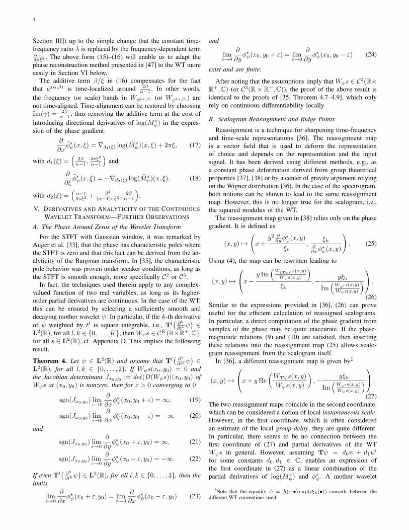
Theorem 4. Let ψ ∈ L2(R) and assume that Tl(∂k

∂tkψ)∈

L2(R), for all l, k ∈ {0, . . . , 2}. If Wψs(x0, y0) = 0 andthe Jacobian determinant Jx0,y0 := det(D(Wψs))(x0, y0) ofWψs at (x0, y0) is nonzero, then for ε > 0 converging to 0

sgn(Jx0,y0) limε→0

∂

∂xφsψ(x0, y0 + ε) =∞, (19)


∂

∂xφsψ(x0, y0 − ε) = −∞ (20)

and


∂

∂yφsψ(x0 + ε, y0) =∞, (21)


∂

∂yφsψ(x0 − ε, y0) = −∞. (22)

If even Tl(∂k

∂tkψ)∈ L2(R), for all l, k ∈ {0, . . . , 3}, then the

limits

limε→0

∂

∂xφsψ(x0 + ε, y0) = lim

ε→0

∂

∂xφsψ(x0 − ε, y0) (23)

and

limε→0

∂

∂yφsψ(x0, y0 + ε) = lim

ε→0

∂

∂yφsψ(x0, y0 − ε) (24)

exist and are finite.

After noting that the assumptions imply that Wψs ∈ C2(R×R+,C) (or C3(R × R+,C)), the proof of the above result isidentical to the proofs of [35, Theorem 4.7–4.9], which onlyrely on continuous differentiability locally.

B. Scalogram Reassignment and Ridge Points

Reassignment is a technique for sharpening time-frequencyand time-scale representations [36]. The reassignment mapis a vector field that is used to deform the representationof choice and depends on the representation and the inputsignal. It has been derived using different methods, e.g., asa constant phase deformation derived from group theoreticalproperties [37], [38] or by a center of gravity argument relyingon the Wigner distribution [36]. In the case of the spectrogram,both notions can be shown to lead to the same reassignmentmap. However, this is no longer true for the scalogram, i.e.,the squared modulus of the WT.

The reassignment map given in [38] relies only on the phasegradient. It is defined as

(x, y) 7→

(x+

y2 ∂∂yφ

sψ(x, y)

ξb,

ξb∂∂xφ

sψ(x, y)

). (25)

Using (4), the map can be rewritten leading to

(x, y) 7→

x− y Im(W(Tψ)′s(x,y)

Wψs(x,y)

)ξb

,− yξb

Im(Wψ′s(x,y)

Wψs(x,y)

) .

(26)Similar to the expressions provided in [36], (26) can proveuseful for the efficient calculation of reassigned scalograms.In particular, a direct computation of the phase gradient fromsamples of the phase may be quite inaccurate. If the phase-magnitude relations (9) and (10) are satisfied, then insertingthese relations into the reassignment map (25) allows scalo-gram reassignment from the scalogram itself.

In [36], a different reassignment map is given by2

(x, y) 7→

x+ yRe

(WTψs(x, y)

Wψs(x, y)

),− yξb

Im(Wψ′s(x,y)

Wψs(x,y)

) .

(27)The two reassignment maps coincide in the second coordinate,which can be considered a notion of local instantaneous scale.However, in the first coordinate, which is often consideredan estimate of the local group delay, they are quite different.In particular, there seems to be no connection between thefirst coordinate of (27) and partial derivatives of the WTWψs in general. However, assuming Tψ = d0ψ + d1ψ

′

for some constants d0, d1 ∈ C, enables an expression ofthe first coordinate in (27) as a linear combination of thepartial derivatives of log(Ms

ψ) and φsψ . A mother wavelet

2Note that the equality ψ = h(−•) exp(iξb(•)) converts between thedifferent WT conventions used.


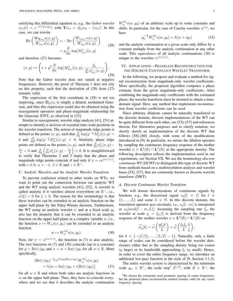
satisfying this differential equation is, e.g., the Gabor waveletψG(t) = e−t

2/2+iξbt, with TψG = iξbψG − (ψG)′. In thiscase, we can rewrite

Re

(WTψGs(x, y)

WψGs(x, y)

)= −Re

(W(ψG)′s(x, y)

WψGs(x, y)

)= y

∂

∂xlog(Ms

ψG)(x, y)

(28)

and therefore (27) becomes

(x, y) 7→

(x+ y2

∂

∂xlog(Ms

ψG)(x, y),

ξb∂∂xφ

sψG

(x, y)

).

(29)Note that the Gabor wavelet does not vanish at negativefrequencies. However, the proof of Theorem 1 does not relyon this property, such that the derivation of (29) from (27)remains valid.

The expression of the first coordinate in (29) is not toosurprising, since DyψG is simply a dilated, modulated Gaus-sian, and thus this expression could also be obtained using thereassignment operators and phase-magnitude relationship forthe Gaussian STFT, as observed in [33].

Similar to reassignment, wavelet ridge analysis [41], [51] at-tempts to identify a skeleton of essential time-scale positions inthe wavelet transform. The notion of magnitude ridge points isdefined as the points (x, y), such that ∂

∂y log(y−12Ms

ψ)(x, y) =

0 and ∂2

∂y2 log(y−12Ms

ψ)(x, y) < 0. Similarly, phase ridgepoints are defined as the points (x, y), such that ∂

∂xφsψ(x, y)−

ξby = 0 and ∂

∂y

(∂∂xφ

sψ(x, y)− ξb

y

)> 0. It is straightforward

to verify that Theorems 2 and 3 imply that the phase andmagnitude ridge points coincide if and only if ψ = cψ(α,β,γ),with c 6= 0, α > −1, β ∈ R and γ ∈ R+.

C. Analytic Wavelets and the Analytic Wavelet Transform

To prevent confusion related to other works on WTs, wewant to point out the connection between our analytic WTand the WT using analytic wavelets [41], [52]. A wavelet iscalled analytic if it vanishes almost everywhere on R−, i.e.,ψ(ξ) = 0 for ξ < 0. The reason for this terminology is thatthese wavelets can be extended to an analytic function on theupper half-plane by the Paley-Wiener theorem. Furthermore,the WT using an analytic wavelet ψ and at a fixed scale y0also has the property that it can be extended to an analyticfunction on the upper half-plane in a complex variable w, i.e.,the function x 7→ Wψs(x, y0) can be extended to an analyticfunction

w 7→W(a)ψ s(w, y0). (30)

Now, for ψ = ψ(α,β,γ), the function in (7) is also analytic.The two functions in (7) and (30) coincide (up to a constant)for y = Re(γ)y0 and x = w + Im(γ)y0 for all w ∈ R. Morespecifically,

(Re(γ)y0)−α2 eiβ log(Re(γ)y0)W

(a)ψ s(w, y0)

= h(w + Im(γ)y0 + i(Re(γ)y0)

)(31)

for all w ∈ R and where both sides are analytic functions inw on the upper half-plane. Thus, they have to coincide every-where and we see that h describes the analytic continuation

W(a)ψ s(w, y0) of an arbitrary scale up to some constants and

shifts. In particular, for the case of Cauchy wavelets ψ(α), wehave

y−α20 W

(a)ψ s(w, y0) = h(w + iy0) (32)

and the analytic continuation at a given scale only differs by aconstant multiple from the analytic continuation at any otherscale. This equivalence of all analytic continuations (30) isunique to the wavelets ψ(α,β,γ).

VI. APPLICATION—PHASELESS RECONSTRUCTION FORTHE DISCRETE CONTINUOUS WAVELET TRANSFORM

In the following, we propose and evaluate a method for sig-nal reconstruction from magnitude-only wavelet coefficients.More specifically, the proposed algorithm computes a phaseestimate from the given magnitude-only coefficients. Aftercombining the magnitude-only coefficients with the estimatedphase, the wavelet transform must be inverted to obtain a time-domain signal. Here, any method that implements reconstruc-tion from wavelet coefficients can be used.

Since arbitrary dilations cannot be naturally transferred tothe discrete domain, discrete implementations of the WT canbe quite different from each other, see [53]–[57] and referencestherein. For illustrative purposes and to clarify notation, weshortly sketch an implementation of the discrete WT thatfollows [58]–[60] closely, with some of the modificationsintroduced in [9]. In particular, we mimic the dilation operatorby sampling the continuous frequency response of the motherwavelet ψ ∈ L2(R) ∩ L1(R) at the appropriate density. Thefollowing description reflects the implementation used in ourexperiments, see Section VII. We use the terminology discretecontinuous WT (DCWT) to distinguish this type of discrete WTfrom methods based on a multiresolution analysis and waveletbases [53], [57], that are commonly known as discrete wavelettransform (DWT).

A. Discrete Continuous Wavelet Transform

We will denote discretizations of continuous signals bybrackets, e.g., the discretized signal sd[l] ∈ C for l ∈{1, . . . , L} and some L ∈ N. In this discrete domain, thetranslation operator acts circularly, i.e., sd[l−m] is interpretedas sd[mod(l − m,L)]. Assuming the sampling rate ξs, thewavelet at scale y = ξb/ξ is derived from the frequencyresponse of the mother wavelet ψ ∈ L2(R) ∩ L1(R) as

ψy[k] = ψ

(yξsk

L

)= ψ

(ξbξsL

k

ξ

),

for k ∈ {−bL/2c, . . . , dL/2e − 1}. Naturally, only a finiterange of scales can be considered before the wavelet dete-riorates either due to the sampling density being too coarse(y large) or its bandwidth approaching ξs (y small). Hence,in order to cover the entire frequency range, we introduce anadditional low-pass function in the style of [9, Section 3.1.2].

The entire wavelet system is characterized by the minimumscale ym ∈ R+, the scale step3 21/B , with B ∈ R+, the

3We choose the commonly used geometric spacing of center frequencies,but the proposed phase reconstruction method remains valid for any centerfrequency spacing.

6

number of scales K ∈ N, and the decimation factor ad ∈ N,with ad|L. The corresponding scaled and shifted wavelets aregiven as

ψn,k = Tnadψ2k/Bym (33)

for k ∈ {0, . . . ,K − 1} and n ∈ {0, . . . , L/ad − 1}. Aplateau function Plp ∈ CL, centered at 0, specifies the low-pass function as

ψlp = a−1d PlpΨlp, (34)

where

Ψlp =√

max(Ψ)−Ψ, Ψ =

K−1∑k=0

|ψ0,k|2. (35)

An analysis with the constructed system yields LK/ad com-plex-valued coefficients for the wavelet scales and additionalL/ad real-valued coefficients for the low-pass function, for atotal redundancy of (2K + 1)/ad when analyzing real-valuedsignals. With a slight abuse of terminology, we will from nowon refer to the proportional quantity K/ad as the redundancy.

If ψ is smooth and ad, 1/B are small enough, then theresults in [58] imply that the DCWT is invertible. Inversioncan be achieved by interpreting the wavelet transform as afilter bank analysis and invoking the frame theory of uniformfilter banks [61]–[64] to compute a dual filter bank synthesis.This can be done either directly using dual filters ψk, oriteratively [9], [65] using conjugate gradient iterations. Theconsideration of general uniform filter banks is necessary:It is not always possible to find a dual filter bank, whichis required to achieve perfect reconstruction, with waveletstructure. Nonetheless, the dual filter bank shares the numberof channels K + 1 and the decimation factor a of the waveletanalysis.

B. Application to Phaseless Reconstruction

For the phase-magnitude relations presented in Theorem 3to hold, we have to assume a wavelet ψ(α,β,γ) as in (6). Inparticular, we will restrict to the case γ = 1 for simplicityand drop the superscript (α, β) for notational convenience.For the WT and the phase-magnitude relations, we will usethe convention introduced in Section IV. The generalization tothe full class of wavelets described by (6) is straightforward.

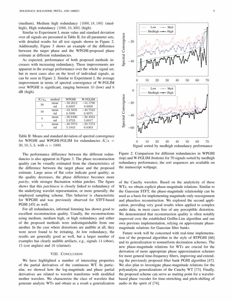
Note that Theorem 3 provides only the phase-derivative andindeed reconstruction can at best be expected to be accurateup to a global phase factor. Furthermore, the reconstructionquality is expected to be worse for low-magnitude areasand thus the proposed algorithm only reconstructs the phasedown to a certain magnitude-threshold. Coefficients below thatthreshold are expected to have little effect on the synthesis andcan thus be assigned a random phase. As a consequence ofthe local, adaptive integration scheme, the reconstructed phaseis in fact only expected to be consistent locally with changesby a constant phase factor between these local components.On audio signals, such as the chosen corpus of test data, thischange is not expected to have notable perceptual effects.Nonetheless, it is visible in the phase difference (betweenoriginal and reconstructed phase) in Fig. 3. At low redundancy,which is not well-suited for phase reconstruction in general,

the phase distortion may become more severe (see the lowerright corner in Fig. 3), sometimes leading to perceivabledistortion.

Assume that the continuous-time signal s is approximatelyband- and time-limited on [0, ξs) and [0, L/ξs), respectively.Then, with sd[l] = s(l/ξs), for l ∈ {0, . . . , L−1}, ad = aξs ∈N, and ξk = 2−k/Bξb/ym, we obtain the approximation

Ms[n, k] := |〈sd, ψn,k〉| ≈ ξsMsψ(na, ξk). (36)

Note that, after taking the logarithmic derivative of (36), thenormalization by ξs becomes irrelevant.

Hence, we have

∂

∂xφsψ(na, ξk) =

4πξ2kα− 1

∂

∂ξlog(Ms

ψ)(na, ξk) + 2πξk

≈ ∆φ,x,sψ [n, k] :=

4πξ2kα− 1

∆k(log(Ms))[n, k] + 2πξk, (37)

and∂

∂ξφsψ(na, ξk) =− α− 1

4πξ2k

∂

∂xlog(Ms

ψ)(na, ξk) +β

ξk

≈ ∆φ,ξ,sψ [n, k] :=− α− 1

4πξ2k∆n(log(Ms))[n, k] +

β

ξk. (38)

Here, ∆n and ∆k are appropriate discrete differentiationschemes. For ∆n, we can use centered differences, i.e.,

∆n(M)[n, k] :=ξs(M [n+ 1, k]−M [n− 1, k])

2ad. (39)

The sampling step in the scale coordinate changes depends onk and weighted centered differences can be used:

∆k(M)[n, k] :=M [n, k + 1]−M [n, k]

2(ξk+1 − ξk)

+M [n, k]−M [n, k − 1]

2(ξk − ξk−1). (40)

Now, from ∆φ,x,sψ and ∆φ,ξ,s

ψ , an estimate of the phase ofWψs at the sampling points {(na, ξk)}n,k can be obtainedusing a quadrature rule considering the variable sampling in-tervals. That even simple 1-dimensional trapezoidal quadratureprovides satisfactory results is illustrated by our experiments,see Section VII.

The integration itself can be performed by a slightly modi-fied Phase Gradient Heap Integration (PGHI) algorithm [45],[47], [66], see Algorithm 1, using, e.g., the following inte-gration rule on the set of neighbors (nn, kn) ∈ Nn,k :={(n± 1, k), (n, k ± 1)} of (n, k)

is(φsψ)est[nn, kn]

= (φsψ)est[n, k] +ξkn − ξk

2

(∆φ,ξ,sψ [n, k] + ∆φ,ξ,s

ψ [nn, kn])

+ad(nn − n)

2ξs

(∆φ,x,sψ [n, k] + ∆φ,x,s

ψ [nn, kn]). (41)

When inserting (39) and (40) into (41), the absolute scaleof the center frequencies ξk and sampling rate ξs becomesunimportant and only their ratio enters the quadrature (41).Hence, by considering relative frequencies ξk/ξs, the algo-rithm is valid independent of the assumed sampling rate.


Algorithm 1: Wavelet Phase Gradient Heap IntegrationInput: Magnitude Ms of wavelet coefficients, estimates

∆φ,x,sψ and ∆φ,ξ,s

ψ of the partial phase derivatives,relative tolerance tol .

Output: Phase estimate (φsψ)est.1 abstol ← tol ·max (Ms[n, k]);2 Create set I = {(n, k) : Ms[n, k] > abstol};3 Assign random values to (φsψ)est(n, k) for k /∈ I;4 Construct a self-sorting max heap [67] for (n, k) pairs;5 while I is not ∅ do6 if heap is empty then7 Move (nm, km) = arg max

(n,k)∈I(Ms[n, k]) from I

into the heap;8 (φsψ)est(nm, km)← 0;9 end

10 while heap is not empty do11 (n, k)← remove the top of the heap;12 foreach (nn, kn) in Nn,k ∩ I do13 Compute (φsψ)est(nn, kn) by means of (41);14 Move (nn, kn) from I into the heap;15 end16 end17 end

Once the phase estimate (φsψ)est has been computed, itis combined with the magnitude by Ws,est := Mse

i(φsψ)est .Subsequently, a time-domain signal can be synthesized asusual, e.g., using a dual filter bank.

VII. EXPERIMENTS

To test and evaluate the proposed method, we performed twoexperiments, described and discussed below. Both experimentswere run on the first 5 seconds of all 70 test signals from theSound Quality Assessment Material recordings for subjectivetests provided by the European Broadcasting Union (SQAMdatabase) [68]. For wavelet analysis and synthesis, we used thefilter bank methods in the open source Large Time-FrequencyAnalysis Toolbox (LTFAT [69], http://ltfat.github.io/), whereour implementation of Wavelet Phase Gradient Heap In-tegration (WPGHI) is available by using the ’wavelet’flag in filterbankconstphase. A function to generatethe wavelet filters and scripts for generating the individualexperiments and figures are provided on the manuscript web-site http://ltfat.github.io/notes/053/, where the resulting audiofiles for all experiment conditions can be found as well.Experimental conditions were restricted to classical Cauchywavelets, i.e., β = 0 and γ = 1.

Thus, the WT parameters used in the experiments are(α, ad,K), where α is the order of the Cauchy wavelet, adis the decimation step and K is the number of frequencychannels (or scales) used before adding the lowpass filter.As quantitative error measure, we employ (wavelet) spectralconvergence [70], i.e., the relative mean squared error (in dB)

between the wavelet coefficient magnitude of the target signalst and the proposed solution sp:

SC(sp, st) = 20 log10

‖Msp −Mst‖‖Mst‖

.

It should be noted that the wavelet coefficient magnitude inthe above formula was computed using the same parameter set(α, ad,K) for which phaseless reconstruction was attempted.4

A. Experiment I—Comparison to Previous Methods

To study the performance of the proposed algorithm incomparison with previous methods for phaseless recoveryfrom wavelet coefficients, we selected three settings of theWT parameters (α, ad,K). For all settings, the channel centerfrequencies where geometrically spaced in ξs

20 · [2−6, 23.3]. We

considered the following tuples of parameters: (30, 5, 100),(300, 12, 240), and (3000, 20, 400). Here, the ratio K/ad = 20was fixed in all cases, but ad and K were adjusted toaccommodate for bandwidth variations with changing α.

The dimensionality of the considered audio data renders asystematic comparison to existing implementations of someestablished methods, e.g., [16], [19] unfeasible, such thatwe resort to fast Griffin-Lim [20], [23] as baseline method.We compare four different methods: wavelet PGHI (WPGHI,proposed), filter bank PGHI (FBPGHI, [47]), fast Griffin-Lim with random initialization (R-FGLIM, [23]) and fastGriffin-Lim initialized with the result of WPGHI (W-FGLIM,proposed). Fast Griffin-Lim was restricted to at most 150iterations.5 Spectral convergence of the four methods on alltest signals is shown in Figure 1 for the different parametersets (α, ad,K). The means and standard deviation across allsignals, for every method and parameters set are shown inTable I.

It can be seen that on average, plain WPGHI (proposed)outperforms both R-FGLIM and FBPGHI on all parametersets, although FBPGHI approaches the other methods forlarger values of α. Moreover, W-FGLIM (proposed) showssignificant improvements over either WPGHI or R-FGLIM.Looking at the individual signals more closely, we see inFigure 1 that there are only very few cases in which R-FGLIMyields a better result than W-FGLIM. For α = 3000, allmethods show comparable performance, with the exceptionof W-FGLIM, which still provides a clear advantage.

The figures and the computed standard deviations bothsuggest that methods that perform well on average are proneto larger performance fluctuation between individual signals.However, there is a small set of signals on which all methodsperform badly, indicating that the fault is with the wavelet

4Although spectral convergence is in some cases sensitive to parameterchanges, preliminary tests showed that, for fixed α, comparable spectralconvergence is achieved with respect to representations with varying adand K. On the other hand, when α is changed as well, then the value ofSC(sp, st) may change dramatically, such that comparing the results acrossdifferent choices of α may be misleading.

5Although we are mainly interested in the reconstruction quality and not incomputational performance, it is worth mentioning that the solutions of plainWPGHI and FBPGHI are computed in a small fraction of the time required forexecuting either R-FGLIM or W-FGLIM, even if, at the cost of reconstructionquality, the maximum number of iterations was significantly reduced.

http://ltfat.github.io/

http://ltfat.github.io/notes/053/

8

representation rather than the method applied for phaselessreconstruction. Notably, signal 65 (corresponding to the right-most signal in Figures 1–2) from the SQAM database, which,in the considered range, only contains a sustained, extremelylow-pitched note is badly resolved by the employed WT andyields the worst spectral convergence of all signals, for any ofthe employed methods.

Informal listening showed that, for α = 3000 and anuntrained listener, the obtained reconstructions are mostlyindistinguishable from the original signal. For α = 300and, more prominently, α = 30, FBPGHI often introducesa characteristic pitch-shift, likely due to a wrongly estimatedtime-direction phase derivative, while R-FGLIM suffers fromundesired frequency modulation artifacts; both types of dis-tortion are most easily audible in simple signals, such assignal 1 (sine wave) and 4 (electronic gong) of the SQAMdatabase and not present in the reconstructions provided byWPGHI. For α = 30 and some select cases, e.g., signals 16(clarinet) and 32 (triangle), audible distortions were present inthe solutions by W-FGLIM, but not those by plain WPGHI,indicating that the observed improvement in terms of spectralconvergence does not necessarily provide a perceptual im-provement. To confirm our observations and to form their ownopinion, the reader is invited to visit the manuscript webpagehttp://ltfat.github.io/notes/053/.

As a side note, the audio examples6 provided with [45] haveclearly audible artifacts for signal 54 (male German speech),for STFT-based PGHI and some competing algorithms. Theseartifacts are not present in any of the reconstructions weobtained using WPGHI, R-FGLIM, or W-FGLIM, for anyconsidered parameter set, indicating that in some cases, usageof the WT may provide a genuine advantage over the STFT.

α method WPGHI FBPGHI R-FGLIM W-FGLIM

30 mean −33.9512 −18.2916 −28.9164 −40.2932std 7.7632 2.0358 3.2641 7.0526

300 mean −36.6393 −26.8642 −29.3628 −42.7550std 7.9517 3.4095 4.0747 9.0264

3000 mean −38.5527 −34.8240 −32.0108 −44.9260std 6.7961 5.5137 5.4821 10.6349

Table I: Means and standard deviation of spectral convergencefor the considered methods and parameter sets.

B. Experiment II—Changing the Redundancy

In a second set of experiments, we investigate the influenceof the redundancy K/ad on the performance of the proposedmethods WPGHI and W-FGLIM. For this purpose, we fixedan intermediate value for the order parameter, setting α =1000 and consider redundancies K/ad ∈ {3, 5, 10, 30}. Here,however, the reconstruction quality does not only depend onthe accuracy of WPGHI on the given magnitude coefficients,but also on the robustness of the synthesis by the dual system.This robustness can be quantified by the so-called frame boundratio of the respective wavelet system (for details see [53],[71], [72]).

In the ranges considered and for fixed K/ad, the num-ber K of frequency channels has a larger influence on

6Avalabile at http://ltfat.github.io/notes/040/

0 10 20 30 40 50 60 70

−40

−20

0

Spec

tral

Con

verg

ence

FBPGHI WPGHIR-FGLIM W-FGLIM

0 10 20 30 40 50 60 70

−60

−40

−20

0

Spec

tral

Con

verg

ence


0 10 20 30 40 50 60 70

−60

−40

−20

0

Signal sorted by R-FGLIM performance

Spec

tral

Con

verg

ence


Figure 1: 70 signals for α = 30 (top), α = 300 (middle), andα = 3000 (bottom) sorted by R-FGLIM performance; the sortsequences are available on the manuscript webpage.

WPGHI performance than the decimation step ad, whichwas generally small. On the other hand, the wavelet framebound ratio deteriorates very quickly7 for too large dec-imation steps ad. Hence, the choice of wavelet parame-ters was a trade-off between the two factors with no clearoptimal solution. After some preliminary testing, we fixedthe following parameter sets (α, ad,K): Low redundancy(1000, 30, 90) (low), Medium redundancy (1000, 25, 125)

7Large frame bound ratios also decrease numerical stability, such that audiofile generation from the obtained reconstructions is prone to clipping artifacts.




(medium), Medium high redundancy (1000, 18, 180) (med-high), High redundancy (1000, 10, 300) (high).

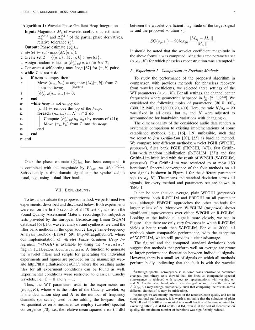
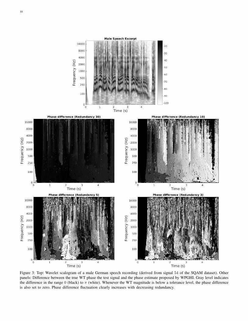
Similar to Experiment I, mean value and standard deviationover all signals are presented in Table II, for all parameter sets,with detailed results for all test signals shown in Figure 2.Additionally, Figure 3 shows an example of the differencebetween the target phase and the WPGHI-proposed phaseestimate at different redundancies.

As expected, performance of both proposed methods in-creases with increasing redundancy. These improvements areapparent in the average performance over the whole signal set,but in most cases also on the level of individual signals, ascan be seen in Figure 2. Similar to Experiment I, the averageimprovement in terms of spectral convergence of W-FGLIMover WPGHI is significant, ranging between 10 (low) and 6dB (high).

K/ad method WPGHI W-FGLIM

30 mean −38.2012 −44.1790std 6.6897 9.8989

10 mean −32.5835 −40.7522std 6.5999 6.9075

5 mean −26.8400 −36.4934std 5.9723 5.6917

3 mean −20.7873 −29.7372std 5.1843 6.6363

Table II: Means and standard deviation of spectral convergencefor WPGHI and WPGHI-FGLIM for redundancies K/a =30, 10, 5, 3, with α = 1000.

The performance difference between the different redun-dancies is also apparent in Figure 3. The phase reconstructionquality can be visually estimated from the characteristics ofthe difference between the target phase and the proposedestimate. Large areas of flat color indicate good quality; asthe quality decreases, the phase difference becomes morepatchy, with stronger fluctuation within patches. The figureshows that this patchiness is closely linked to redundancy ofthe underlying wavelet representation, or more generally, theemployed sampling scheme. This behavior is characteristicfor WPGHI and was previously observed for STFT-basedPGHI [45] as well.

For all redundancies, informal listening has shown good toexcellent reconstruction quality. Usually, the reconstructionsusing medium, medium high, or high redundancy and eitherof the proposed methods were indistinguishable from oneanother. In the case where distortions are audible at all, theywere never found to be irritating. At low redundancy, theresults are generally good as well, but a larger number ofexamples has clearly audible artifacts, e.g., signals 14 (oboe),15 (cor anglais) and 16 (clarinet).

VIII. CONCLUSION

We have highlighted a number of interesting propertiesof the partial derivatives of the continuous WT. In partic-ular, we showed how the log-magnitude and phase partialderivatives are related to wavelet transforms with modifiedmother wavelets. We characterize the class of wavelets thatgenerate analytic WTs and obtain as a result a generalization

0 10 20 30 40 50 60 70

−40

−20

Spec

tral

Con

verg

ence

Low MedMedhigh High

0 10 20 30 40 50 60 70

−60

−40

−20

0

Signal sorted by medhigh redundancy performance

Spec

tral

Con

verg

ence

Low MedMedhigh High

Figure 2: Comparison for different redundancies in WPGHI(top) and W-FGLIM (bottom) for 70 signals sorted by medhighredundancy performance; the sort sequences are available onthe manuscript webpage.

of the Cauchy wavelets. Based on the analyticity of theseWTs, we obtain explicit phase-magnitude relations. Similar tothe Gaussian STFT, the phase-magnitude relationship can beused as a basis for implementing magnitude-only reassignmentand phaseless reconstruction. We explored the second appli-cation, providing very good results when applied to complexaudio data, in most cases free of any perceptible distortion.We demonstrated that reconstruction quality is often notablyimproved over the established Griffin-Lim algorithm and ourown previous implementation, relying on approximate phase-magnitude relations for Gaussian filter banks.

Future work will be concerned with real-time implementa-tion of the proposed algorithm in the style of RTPGHI [66]and its generalization to nonuniform decimation schemes. Thenew phase-magnitude relations for WTs are crucial for thederivation of more appropriate phase approximation schemesfor more general time-frequency filters, improving and extend-ing the previously proposed filter bank PGHI algorithm [47].We also plan to investigate phase-magnitude relations for thepolyanalytic generalizations of the Cauchy WT [73]. Finally,the proposed scheme can serve as starting point for a wavelet-based phase vocoder for time-stretching and pitch-shifting ofaudio in the spirit of [74].

10

Figure 3: Top: Wavelet scalogram of a male German speech recording (derived from signal 54 of the SQAM dataset). Otherpanels: Difference between the true WT phase the test signal and the phase estimate proposed by WPGHI. Gray level indicatesthe difference in the range 0 (black) to π (white). Whenever the WT magnitude is below a tolerance level, the phase differenceis also set to zero. Phase difference fluctuation clearly increases with decreasing redundancy.


ACKNOWLEDGMENTS

We wish to thank Andrés Marafioti for performing a smalllistening test confirming the reported observations on theperceptual quality of the reconstructed audio samples. Further-more, we would like to thank Patrick Flandrin for pointing usto the literature on Klauder wavelets which coincide with theanalyticity inducing wavelets given by (6). Finally, we thankthe reviewers, whose comments helped us improve our resultsand their presentation.

APPENDIX APROOF OF THEOREM 1

Proof. Under the assumption that ψ ∈ L2(R) is continuouslydifferentiable with ψ′,Tψ′ ∈ L2(R), we can exchange dif-ferentiation and integration in (2), see Appendix D. Thus, thepartial derivatives of Wψs can be expressed as

∂

∂xWψs(x, y) = − 1

y√y

∫Rs(t)ψ′

(t− xy

)dt

= −1

yWψ′s(x, y)

(42)

and∂

∂yWψs(x, y)

= − 1

y√y

∫Rs(t)

(ψ(•)

2+ (•)ψ′(•)

)(t− xy

)dt

= −1

y

(Wψs(x, y)

2+WT(ψ′)s(x, y)

)= −1

y

(−Wψs(x, y)

2+W(Tψ)′s(x, y)

). (43)

Here, we used that (Tψ)′ = ψ+Tψ′ and that that the WT isconjugate linear with respect to the chosen wavelet. Using that∂∂x log(Wψs) =

∂∂xWψs

Wψsand similarly for the partial derivative

with respect to y, we obtain for all (x, y) with Wψs(x, y) 6= 0,

∂

∂xlog(Wψs)(x, y) = −1

y

Wψ′s(x, y)

Wψs(x, y)(44a)

∂

∂ylog(Wψs)(x, y) =

1

2y− 1

y

W(Tψ)′s(x, y)

Wψs(x, y). (44b)

Taking real and imaginary parts in (44) results in (3) and (4),respectively.

APPENDIX BPROOF OF THEOREM 2

We first argue that analyticity of h and differentiability of falready imply that ψ satisfies the assumptions in Theorem 1,i.e., ψ is continuously differentiable with ψ,ψ′,Tψ′ ∈ L2(R).To this end, we note that the assumptions imply that Wψs(x−aby, by) must be C∞ in x and y for an arbitrary s ∈ L2(R).The same holds true for Wψs(x, y).

At x = 0 and y = 1, the derivative ∂∂xWψs can be written

as∂

∂xWψs(0, 1) = lim

x0→0

⟨s,ψ −T−x0

ψ

x0

⟩, (45)

which converges for every fixed s ∈ L2(R). Thus, by a variantof the Banach-Steinhaus theorem [75, Ch. II.1, Corollary 2],the limit limx0→0

ψ−T−x0ψx0

represents a continuous linearfunctional and hence, by Riesz representation theorem, anelement ψx in L2(R). Rewriting the derivative for compactlysupported, smooth s alternatively as

∂

∂xWψs(0, 1) = lim

x0→0

⟨s−Tx0s

x0, ψ

⟩= −〈s′, ψ〉 , (46)

we see that ψx is the weak derivative of ψ, i.e., the weakderivative of ψ exists and belongs to L2(R). Repeating the ar-gument for higher derivatives guarantees that weak derivativesof arbitrary order exist and by standard Sobolev embeddingsso do continuous derivatives.

Similarly, the derivative ∂∂yWψs at x = 0 and y = 1 can be

written as∂

∂yWψs(0, 1) = lim

y0→0

⟨s,ψ −D−y0ψ

y0

⟩. (47)

Again we have the convergence limy0→0ψ−D−y0ψ

y0= ψy .

Rewriting the derivative for s ∈ C∞00 alternatively as

∂

∂yWψs(0, 1) = lim

y0→0

⟨s−D1/−y0s

y0, ψ

⟩= 〈s+ Ts′, ψ〉= 〈(Ts)′, ψ〉 . (48)

Now the operator s 7→ Ts′ is well defined for compactlysupported, smooth s with adjoint s 7→ −(Ts)′. Furthermore,ψ is in the domain of this operator because 〈−(Ts)′, ψ〉 =〈s, ψy〉 for all s in a dense subset. Thus, Tψ′ = ψy ∈ L2(R).Hence, we established all assumptions of Theorem 1.

Analyticity of the function h is equivalent to it satisfyingthe CR equations that can be compactly expressed as ∂

∂xh =−i ∂∂yh. To rewrite the CR equations for the function h in (5),we use (42), to obtain

∂

∂xh =

(∂

∂xf(x, y)

)Wψs(x− aby, by)

− f(x, y)

byWψ′s(x− aby, by). (49)

Similarly, by (43), we have

∂

∂yh =

(∂

∂yf(x, y)

)Wψs(x− aby, by)

− f(x, y)

y

(− Wψs(x− aby, by)

2

+W(Tψ)′s(x− aby, by)− aWψ′s(x− aby, by)

)=

(∂

∂yf(x, y) +

f(x, y)

2y

)Wψs(x− aby, by)

− f(x, y)

yW(Tψ)′s(x− aby, by)

+f(x, y)

yaWψ′s(x− aby, by). (50)

Inserting these expressions into the CR equations results in(y ∂∂xf(x, y) + iy ∂

∂yf(x, y)

f(x, y)+i

2

)Wψs(x− aby, by)

12

=1− iabb

Wψ′s(x− aby, by) + iW(Tψ)′s(x− aby, by).

(51)

We note that this condition depends on f only via the functiong(x, y) =

y ∂∂x f(x,y)+iy

∂∂y f(x,y)

f(x,y) + i2 . Moreover, using the

definition of the WT in (51) implies that∫Rs(t)

(g(x, y)ψ

(t− xy

)− 1− iab

bψ′(t− xy

)− i(Tψ)′

(t− xy

))dt = 0

(52)

for all s ∈ L2(R) and thus

g(x, y)ψ

(t− xy

)− 1− iab

bψ′(t− xy

)− i(Tψ)′

(t− xy

)= 0 (53)

as a function of t in L2(R). In particular, this implies thatg(x, y) must be a constant w ∈ C and further

wψ − 1 + iab

bψ′ + i(Tψ)′ = 0 . (54)

To solve this differential equation, it is more convenient toconsider the Fourier transformed equivalent of (54). Using thestandard properties of the Fourier transform ψ′ = 2πiTψ andTψ = −(2πi)−1(ψ)′, this is easily seen to be given by

wψ − 2πi1 + iab

bTψ − iT(ψ)′ = 0. (55)

We first note that our assumption ψ(ξ) = 0 for ξ < 0 satisfiesthis differential equation on this domain. For ξ > 0 and ψ 6= 0,we can easily solve the differential equation by rewriting

(ψ)′(ξ)

ψ(ξ)=w

iξ− 2π

1 + iab

b, (56)

which gives

ψ(ξ) = ce−iw log ξe−2π1+iabb ξ

= cξ− Im(w)e−2π(1b+ia)ξe−iRe(w) log ξ (57)

for an arbitrary constant c ∈ C. To obtain the parameters usedin the theorem, we substitute − Im(w) = α−1

2 , 1b = Re(γ),

a = Im(γ), and Re(w) = −β. Based on our assumptions, weobtain the constraints Re(γ) > 0 and α > −1 to guaranteeψ ∈ L2(R).

APPENDIX CPROOF OF THEOREM 3

We can use the CR equations to obtain relationships be-tween the derivatives of real and imaginary parts of the WT,which we will show to result in (11) and (12). For an arbitraryanalytic function h = u + iv the CR equations hold and aregiven by ∂

∂xu = ∂∂yv and ∂

∂yu = − ∂∂xv. Writing h = Meiφ,

the CR equations imply that

∂

∂xφ = − ∂

∂ylogM (58)

and∂

∂yφ =

∂

∂xlogM. (59)

Using (58) and (59) for the function given by (7), yields

∂

∂x

(φsψ

(x− Im(γ)

Re(γ)y,

y

Re(γ)

)+ β log y

)= − ∂

∂ylog

(y−

α2 Ms

ψ

(x− Im(γ)

Re(γ)y,

y

Re(γ)

))(60)

and∂

∂y

(φsψ

(x− Im(γ)

Re(γ)y,

y

Re(γ)

)+ β log y

)=

∂

∂xlog

(y−

α2 Ms

ψ

(x− Im(γ)

Re(γ)y,

y

Re(γ)

)). (61)

These are equivalent to

∂

∂xφsψ =

α

2yRe(γ)− 1

Re(γ)

∂

∂ylog(Msψ

)+

Im(γ)

Re(γ)

∂

∂xlog(Msψ

)(62)

and

− Im(γ)

Re(γ)

∂

∂xφsψ +

1

Re(γ)

∂

∂yφsψ +

β

yRe(γ)=

∂

∂xlog(Msψ

).

(63)Inserting (62) into (63) finally results in

− Im(γ)

Re(γ)

(α

2yRe(γ)− 1

Re(γ)

∂

∂ylog(Msψ

)+

Im(γ)

Re(γ)

∂

∂xlog(Msψ

))+

1

Re(γ)

∂

∂yφsψ +

β

yRe(γ)

=∂

∂xlog(Msψ

), (64)

which is equivalent to

Re(γ)∂

∂yφsψ =

α Im(γ)

2y− β

y+ |γ|2 ∂

∂xlog(Msψ

)− Im(γ)

∂

∂ylog(Msψ

). (65)

This concludes the proof.

APPENDIX DON DIFFERENTIABILITY OF THE WAVELET TRANSFORM

Denote by Φz and Ψz the difference operators

Φzψ =Tzψ − ψ

zand Ψzψ =

D1+(z−1)ψ − ψz − 1

,

and note that∂

∂xWψs(x, y) = lim

x0→0

Wψs(x+ x0, y)−Wψs(x, y)

x0

= limx0→0

1

y

⟨s,TxDy(Φx0/yψ)

⟩,

as well as∂

∂yWψs(x, y) = lim

y0→0

Wψs(x, y + y0)−Wψs(x, y)

y0

= limy0→0

1

y

⟨s,TxDy(Ψ1+y0/yψ)

⟩,


provided that the right-hand sides converge.We first show that, for z → 0

Φzψ → −ψ′ and Ψ1+zψ → −(ψ/2 + Tψ′) (66)

as functions in L2(R), provided that ψ, ψ′, and Tψ′ areelements of L2(R).

Since ψ′ is assumed to be in L2(R), there is for everyε > 0 an rε > 0, such that

∥∥ψ′χR\Brε (0)∥∥ < ε. Moreover, by

the fundamental theorem of calculus,

|Φzψ(t) + ψ′(t)| =∣∣∣∣∫ t−zt

ψ′(s) ds

z+ ψ′(t)

∣∣∣∣=

∣∣∣∣− ∫ 1

0

ψ′(t− sz) + ψ′(t) ds

∣∣∣∣ (67)

Using (67), we obtain∥∥∥(Φzψ + ψ′)χR\Brε+|z|(0)

∥∥∥2≤∫R\Brε+|z|(0)

(∫ 1

0

|ψ′(t− sz)− ψ′(t)| ds)2

dt

≤∫R\Brε+|z|(0)

∫ 1

0

3|ψ′(t− sz)|2 + 3|ψ′(t)|2 ds dt

< 6ε2 (68)

where we used Jensen’s inequality and Fubini’s theorem.Furthermore, we have |ψ′(t − s) − ψ′(t)| < εr(|s|) for all|t| < r and |s| < 1 by uniform continuity of ψ′ on thecompact set Br+1(0), where εr(δ) ↘ 0 for δ → 0. Thus,similar to (68), we obtain∥∥∥(Φzψ + ψ′)χ

Brε+|z|(0)

∥∥∥2 < 2(rε + |z|)ε2rε+1(|z|) (69)

for |z| < 1. Finally, for every ε, there is a zε ∈ (0, 1), such thatεrε+1(zε) < ε/

√2(rε + 1), which implies ‖Φzψ+ψ′‖ <

√7ε

for all |z| ≤ zε.A similar, but slightly more complicated argument shows

that Ψ1+zψ → −(ψ/2 + Tψ′), provided ψ,Tψ′ ∈ L2(R).Here, we start with an rε > 0, such that ‖Tψ′χR\Brε (0)

‖ < ε

and ‖ψχR\Brε (0)‖ < ε. As above, we use the fundamental

theorem of calculus to obtain

|Ψ1+zψ(t) + ψ(t)/2 + Tψ′(t)|

=

∣∣∣∣∣1

(1+z)1/2ψ(

t1+z

)− ψ(t)

z+ψ(t)

2+ tψ′(t)

∣∣∣∣∣=

∣∣∣∣∣∫ z0

[1

(1+•)1/2ψ(

t1+•)]′

(s) ds

z+ψ(t)

2+ tψ′(t)

∣∣∣∣∣=

∣∣∣∣∣−∫ z

0

12ψ(

t1+s

)+ t

1+sψ′( t

1+s

)(1 + s)3/2z

ds+ψ(t)

2+ tψ′(t)

∣∣∣∣∣=

∣∣∣∣∣−∫ 1

0

12ψ(

t1+sz

)+ t

1+szψ′( t

1+sz

)(1 + sz)3/2

+ψ(t)

2+ tψ′(t) ds

∣∣∣∣∣≤∫ 1

0

∣∣∣∣∣ 12ψ(

t1+sz

)(1 + sz)3/2

− ψ(t)

2

∣∣∣∣∣+

∣∣∣∣∣ t1+szψ

′( t1+sz

)(1 + sz)3/2

− tψ′(t)

∣∣∣∣∣ ds(70)

Similar to (68), this results in∥∥∥(Ψ1+zψ + ψ/2 + Tψ′)χR\B(1+|z|)rε (0)

∥∥∥2 < 16ε2.

Furthermore, we can bound for t ∈ B2r(0)∣∣∣∣∣ 12ψ(

t1+s

)(1 + s)3/2

− ψ(t)

2

∣∣∣∣∣≤ 1

2|(1 + s)3/2|

∣∣∣∣∣ψ(

t

1 + s

)− ψ(t)

∣∣∣∣∣+|ψ(t)|

2

∣∣∣∣∣ 1

(1 + s)3/2− 1

∣∣∣∣∣≤ εr(t|s|) +

|ψ(t)|2

εr(|s|) (71)

for any |s| ≤ 1/2, where εr(δ)→ 0 monotonically for δ → 0.Analogously, we obtain∣∣∣∣∣ t

1+sψ′( t

1+s

)(1 + s)3/2

− tψ′(t)

∣∣∣∣∣ ≤ 2εr(t|s|) + |ψ(t)|εr(|s|). (72)

Equations (70)–(72) imply∣∣∣∣Ψ1+zψ(t)+ψ(t)

2+Tψ′(t)

∣∣∣∣ ≤ 3εr(t|z|)+2|ψ(t)|εr(|z|) (73)

and thus∥∥∥(Ψ1+zψ +ψ

2+ Tψ′

)χB(1+|z|)rε (0)

∥∥∥<√

4rε

(3 + 2 sup

t∈B2rε(0)

|ψ(t)|)εrε(2rε|z|

). (74)

for |z| < 1/(4rε) and where we assumed for simplicity 2rε >1. Again, choosing |z| sufficiently small implies the proposedconvergence.

Thus, we finished the proof of (66), which implies⟨s, limx0→0

TxDy(Φx0/yψ)

⟩= −〈s,TxDyψ

′〉

and⟨s, limy0→0

TxDy(Ψ1+y0/yψ)

⟩= −〈s,TxDy(ψ/2 + Tψ′)〉 .

Because convergence is in L2(R), we can exchange limit andintegral by continuity of the inner product.

Clearly, this argument can be repeated to obtain higher orderderivatives, provided that ψ has sufficient regularity and decay.

REFERENCES

[1] R. D. Nowak, “Wavelet-based Rician noise removal for magnetic reso-nance imaging,” IEEE Trans. Image Process., vol. 8, no. 10, pp. 1408–1419, Oct. 1999.

[2] S. Chaplot, L. M. Patnaik, and N. R. Jagannathan, “Classification ofmagnetic resonance brain images using wavelets as input to supportvector machine and neural network,” Biomed. Signal Process. Control,vol. 1, no. 1, pp. 86–92, Jan. 2006.

[3] A. Marec, J.-H. Thomas, and R. El Guerjouma, “Damage characteriza-tion of polymer-based composite materials: Multivariable analysis andwavelet transform for clustering acoustic emission data,” Mech. Syst.Sig. Process., vol. 22, no. 6, pp. 1441–1464, Aug. 2008.

[4] J. Cusido, J. A. Rosero, L. Romeral, J. A. Ortega, and A. Garcia, “Faultdetection in induction machines using power spectral density in waveletdecomposition,” IEEE Trans. Ind. Electron., vol. 55, no. 2, pp. 633–643,Feb. 2008.

14

[5] S. G. Chang, B. Yu, and M. Vetterli, “Adaptive wavelet thresholding forimage denoising and compression,” IEEE Trans. Image Process., vol. 9,no. 9, pp. 1532–1546, Sep. 2000.

[6] M. Antonini, M. Barlaud, P. Mathieu, and I. Daubechies, “Image codingusing wavelet transform,” IEEE Trans. Image Process., vol. 1, no. 2, pp.205–220, Apr. 1992.

[7] O. Yilmaz and S. Rickard, “Blind separation of speech mixtures viatime-frequency masking,” IEEE Trans. Signal Process., vol. 52, no. 7,pp. 1830–1847, Jul. 2004.

[8] S. Chu, S. Narayanan, and C.-C. J. Kuo, “Environmental sound recog-nition with time–frequency audio features,” IEEE Audio, Speech, Lan-guage Process., vol. 17, no. 6, pp. 1142–1158, Aug. 2009.

[9] T. Necciari, N. Holighaus, P. Balazs, Z. Pruša, P. Majdak, and O. Derrien,“Audlet filter banks: A versatile analysis/synthesis framework usingauditory frequency scales,” Appl. Sci., vol. 8, no. 1(96), Jan. 2018.

[10] S. Mallat and I. Waldspurger, “Phase retrieval for the Cauchy wavelettransform,” J. Fourier Anal. Appl., vol. 21, no. 6, pp. 1251–1309, Dec.2015.

[11] R. Balan, P. Casazza, and D. Edidin, “On signal reconstruction withoutphase,” Appl. Comput. Harmon. Anal., vol. 20, no. 3, pp. 345–356, May2006.

[12] A. S. Bandeira, J. Cahill, D. G. Mixon, and A. A. Nelson, “Saving phase:Injectivity and stability for phase retrieval,” Appl. Comput. Harmon.Anal., vol. 37, no. 1, pp. 106–125, Jul. 2014.

[13] R. Alaifari, I. Daubechies, P. Grohs, and R. Yin, “Stable phase retrievalin infinite dimensions,” Found. Comput. Math., 2018.

[14] R. Alaifari, I. Daubechies, P. Grohs, and G. Thakur, “Reconstructingreal-valued functions from unsigned coefficients with respect to waveletand other frames,” J. Fourier Anal. Appl., vol. 23, no. 6, pp. 1480–1494,Dec. 2017.

[15] R. Alaifari and P. Grohs, “Phase retrieval in the general setting ofcontinuous frames for Banach spaces,” SIAM J. Math. Anal., vol. 49,no. 3, pp. 1895–1911, 2017.

[16] I. Waldspurger, “Phase retrieval for wavelet transforms,” IEEE Trans.Inf. Theory, vol. 63, no. 5, pp. 2993–3009, May 2017.

[17] J. R. Fienup, “Phase retrieval algorithms: a comparison,” Appl. Opt.,vol. 21, no. 15, pp. 2758–2769, Aug. 1982.

[18] R. W. Gerchberg and W. O. Saxton, “A practical algorithm for thedetermination of the phase from image and diffraction plane pictures,”Optik, vol. 35, no. 2, pp. 237–246, 1972.

[19] E. J. Candes, T. Strohmer, and V. Voroninski, “Phaselift: Exact andstable signal recovery from magnitude measurements via convex pro-gramming,” Commun. Pure Appl. Math., vol. 66, no. 8, pp. 1241–1274,Aug. 2013.

[20] D. Griffin and J. Lim, “Signal estimation from modified short-timeFourier transform,” IEEE Trans. Acoust., Speech, Signal Process.,vol. 32, no. 2, pp. 236–243, Apr. 1984.

[21] Y. Shechtman, A. Beck, and Y. C. Eldar, “GESPAR: Efficient phaseretrieval of sparse signals,” IEEE Trans. Signal Process., vol. 62, no. 4,pp. 928–938, Feb. 2014.

[22] Y. Shechtman, Y. C. Eldar, O. Cohen, H. N. Chapman, J. Miao,and M. Segev, “Phase retrieval with application to optical imaging: acontemporary overview,” IEEE Signal Process. Mag., vol. 32, no. 3, pp.87–109, May 2015.

[23] N. Perraudin, P. Balazs, and P. L. Sondergaard, “A fast Griffin-Limalgorithm,” in Proc. IEEE Appl. Sig. Process. Audio Acoustics, NewPaltz, NY, USA, Oct. 2013.

[24] E. Moulines and F. Charpentier, “Pitch-synchronous waveform pro-cessing techniques for text-to-speech synthesis using diphones,” Speechcommunication, vol. 9, no. 5-6, pp. 453–467, Dec. 1990.

[25] Y. Wang, R. Skerry-Ryan, D. Stanton, Y. Wu, R. J. Weiss, N. Jaitly,Z. Yang, Y. Xiao, Z. Chen, S. Bengio et al., “Tacotron: Towards end-to-end speech synthesis,” arXiv preprint arXiv:1703.10135, 2017.

[26] A. Marafioti, N. Holighaus, N. Perraudin, and P. Majdak, “Adversarialgeneration of time-frequency features with application in audio synthe-sis,” arXiv preprint arXiv:1902.04072, 2019.

[27] T. Virtanen, “Monaural sound source separation by nonnegative matrixfactorization with temporal continuity and sparseness criteria,” IEEEAudio, Speech, Language Process., vol. 15, no. 3, pp. 1066–1074, Mar.2007.

[28] F. R. Bach and M. I. Jordan, “Learning spectral clustering, withapplication to speech separation,” J. Mach. Learn. Res., vol. 7, pp. 1963–2001, Oct. 2006.

[29] J. Bruna, P. Sprechmann, and Y. LeCun, “Source separation withscattering non-negative matrix factorization,” in Proc. IEEE Int. Conf.Acoust. Speech Signal Process. South Brisbane, Australia: IEEE, 2015,pp. 1876–1880.

[30] E. Moulines and J. Laroche, “Non-parametric techniques for pitch-scaleand time-scale modification of speech,” Speech communication, vol. 16,no. 2, pp. 175–205, Feb. 1995.

[31] J. Laroche and M. Dolson, “Improved phase vocoder time-scale modifi-cation of audio,” IEEE Trans. Speech Audio Process., vol. 7, no. 3, pp.323–332, May 1999.

[32] Z. Pruša and N. Holighaus, “Phase vocoder done right,” in Proc. Eur.Signal Process. Conf. EUSIPCO, Kos island, Greece, Aug. 2017, pp.976–980.

[33] F. Auger, E. Chassande-Mottin, and P. Flandrin, “On phase-magnituderelationships in the short-time Fourier transform,” IEEE Signal Process.Lett., vol. 19, no. 5, pp. 267–270, May 2012.

[34] M. R. Portnoff, “Magnitude-phase relationships for short-time Fouriertransforms based on Gaussian analysis windows,” in Proc. IEEE Int.Conf. Acoust. Speech Signal Process., vol. 4, Washington, D. C., USA,Apr 1979, pp. 186–189.

[35] P. Balazs, D. Bayer, F. Jaillet, and P. Søndergaard, “The pole behavior ofthe phase derivative of the short-time Fourier transform,” Appl. Comput.Harmon. Anal., vol. 40, no. 3, pp. 610–621, May 2016.

[36] F. Auger and P. Flandrin, “Improving the readability of time-frequencyand time-scale representations by the reassignment method,” IEEETrans. Signal Process., vol. 43, no. 5, pp. 1068–1089, May 1995.

[37] L. Daudet, M. Morvidone, and B. Torresani, “Time-frequency andtime-scale vector fields for deforming time-frequency and time-scalerepresentations,” in Proc. SPIE, vol. 3813, San Diego, CA, USA, Jul.1999.

[38] M. Morvidone and B. Torresani, “Variations on Hough-wavelet trans-forms for time-frequency chirp detection,” in Proc. SPIE, vol. 5207,Nov. 2003.

[39] F. Auger, P. Flandrin, Y.-T. Lin, S. McLaughlin, S. Meignen, T. Oberlin,and H.-T. Wu, “Time-frequency reassignment and synchrosqueezing: Anoverview,” IEEE Signal Process. Mag., vol. 30, no. 6, pp. 32–41, Nov.2013.

[40] I. Daubechies, J. Lu, and H.-T. Wu, “Synchrosqueezed wavelet trans-forms: An empirical mode decomposition-like tool,” Appl. Comput.Harmon. Anal., vol. 30, no. 2, pp. 243–261, Mar. 2011.

[41] J. M. Lilly and S. C. Olhede, “On the analytic wavelet transform,” IEEETrans. Inf. Theory, vol. 56, no. 8, pp. 4135–4156, Aug. 2010.

[42] I. Daubechies and T. Paul, “Time-frequency localisation operators—ageometric phase space approach: II The use of dilations,” Inverse Prob.,vol. 4, no. 3, pp. 661–680, Aug. 1988.

[43] P. Flandrin, “Separability, positivity, and minimum uncertainty in time-frequency energy distributions,” J. Math. Phys., vol. 39, no. 8, pp. 4016–4040, Aug. 1998.

[44] G. Ascensi and J. Bruna, “Model space results for the Gabor and wavelettransforms,” IEEE Trans. Inf. Theory, vol. 55, no. 5, pp. 2250–2259, May2009.

[45] Z. Pruša, P. Balazs, and P. L. Søndergaard, “A noniterative method forreconstruction of phase from STFT magnitude,” IEEE Audio, Speech,Language Process., vol. 25, no. 5, May 2017.

[46] Z. Pruša and P. L. Søndergaard, “Real-time spectrogram inversion usingphase gradient heap integration,” in Proc. Int. Conf. Digital AudioEffects, Brno, Czech Republic, Sep. 2016.

[47] Z. Pruša and N. Holighaus, “Non-iterative filter bank phase (re)construc-tion,” in Proc. Eur. Signal Process. Conf. EUSIPCO, Kos island, Greece,Aug. 2017, pp. 952–956.

[48] D. J. Nelson, “Cross-spectral methods for processing speech,” J. Acoust.Soc. Am., vol. 110, no. 5, pp. 2575–2592, Nov. 2001.

[49] ——, “Instantaneous higher order phase derivatives,” Digital SignalProcess., vol. 12, no. 2–3, pp. 416–428, 2002.

[50] F. Auger, E. Chassande-Mottin, and P. Flandrin, “Making reassignmentadjustable: The Levenberg-Marquardt approach,” in Proc. IEEE Int.Conf. Acoust. Speech Signal Process., Kyoto, Japan, Mar. 2012, pp.3889–3892.

[51] N. Delprat, B. Escudié, P. Guillemain, R. Kronland-Martinet,P. Tchamitchian, and B. Torresani, “Asymptotic wavelet and Gaboranalysis: Extraction of instantaneous frequencies,” IEEE Trans. Inf.Theory, vol. 38, no. 2, pp. 644–664, Mar. 1992.

[52] J. M. Lilly and S. C. Olhede, “Generalized Morse wavelets as asuperfamily of analytic wavelets,” IEEE Trans. Signal Process., vol. 60,no. 11, pp. 6036–6041, Nov. 2012.

[53] S. Mallat, A Wavelet Tour of Signal Processing: The Sparse Way, 3rd ed.Burlington, MA: Academic press, 2008.

[54] O. Rioul and P. Duhamel, “Fast algorithms for discrete and continuouswavelet transforms,” IEEE Trans. Inf. Theory, vol. 38, no. 2, pp. 569–586, Mar. 1992.


[55] M. Unser, A. Aldroubi, and S. J. Schiff, “Fast implementation of thecontinuous wavelet transform with integer scales,” IEEE Trans. SignalProcess., vol. 42, no. 12, pp. 3519–3523, Dec. 1994.

[56] M. J. Shensa, “The discrete wavelet transform: Wedding the a trous andMallat algorithms,” IEEE Trans. Signal Process., vol. 40, no. 10, pp.2464–2482, Oct. 1992.

[57] Z. Pruša, P. L. Søndergaard, and P. Rajmic, “Discrete wavelet transformsin the large time-frequency analysis toolbox for Matlab/GNU Octave,”ACM Trans. Math. Softw., vol. 42, no. 4, pp. 32:1–32:23, Jun. 2016.

[58] P. Balazs, M. Dörfler, F. Jaillet, N. Holighaus, and G. Velasco, “Theory,implementation and applications of nonstationary Gabor frames,” J.Comput. Appl. Math., vol. 236, no. 6, pp. 1481–1496, Oct. 2011.

[59] N. Holighaus, M. Dörfler, G. A. Velasco, and T. Grill, “A frameworkfor invertible, real-time constant-Q transforms,” IEEE Audio, Speech,Language Process., vol. 21, no. 4, pp. 775–785, Apr. 2013.

[60] C. Schörkhuber, A. Klapuri, N. Holighaus, and M. Dörfler, “A Matlabtoolbox for efficient perfect reconstruction time-frequency transformswith log-frequency resolution,” in Proc. AES Conf. Semantic Audio,London, UK, Jan. 2014.

[61] H. Bölcskei, F. Hlawatsch, and H. G. Feichtinger, “Frame-theoreticanalysis of oversampled filter banks,” IEEE Trans. Signal Process.,vol. 46, no. 12, pp. 3256–3268, Dec. 1998.

[62] Z. Cvetkovic and M. Vetterli, “Oversampled filter banks,” IEEE Trans.Signal Process., vol. 46, no. 5, pp. 1245–1255, May 1998.

[63] M. Fickus, M. L. Massar, and D. G. Mixon, “Finite frames and filterbanks,” in Finite Frames, P. G. Casazza and G. Kutyniok, Eds. Basel,Switzerland: Birkhäuser, 2013, pp. 337–379.

[64] T. Strohmer, “Numerical algorithms for discrete Gabor expansions,” inGabor Analysis and Algorithms, H. G. Feichtinger and T. Strohmer, Eds.Boston, MA, USA: Birkhäuser, 1998, pp. 267–294.

[65] K. Gröchenig, “Acceleration of the frame algorithm,” IEEE Trans. SignalProcess., vol. 41, no. 12, pp. 3331–3340, Dec. 1993.

[66] Z. Pruša and P. Rajmic, “Toward high-quality real-time signal recon-struction from STFT magnitude,” IEEE Signal Process. Lett., vol. 24,no. 6, pp. 892–896, Jun. 2017.

[67] J. W. J. Williams, “Algorithm 232: Heapsort,” Communications of theACM, vol. 7, no. 6, pp. 347–348, Jun. 1964.

[68] “Tech 3253: Sound Quality Assessment Material recordings for subjec-tive tests,” Eur. Broadc. Union, Geneva, Tech. Rep., Sept. 2008.

[69] Z. Pruša, P. L. Søndergaard, N. Holighaus, C. Wiesmeyr, and P. Balazs,“The large time-frequency analysis toolbox 2.0,” in Sound, Music, andMotion, M. Aramaki, O. Derrien, R. Kronland-Martinet, and S. Ystad,Eds. Cham, Switzerland: Springer, 2014, pp. 419–442.

[70] N. Sturmel and L. Daudet, “Signal reconstruction from STFT magnitude:A state of the art,” in Proc. Int. Conf. Digital Audio Effects, Paris, France,Sep. 2011, pp. 375–386.

[71] O. Christensen, An Introduction to Frames and Riesz Bases. Basel,Switzerland: Birkhäuser, 2016.

[72] I. Daubechies, Ten Lectures on Wavelets. SIAM, 1992.[73] L. D. Abreu, “Superframes and polyanalytic wavelets,” J. Fourier Anal.

Appl., vol. 23, no. 1, pp. 1–20, Feb. 2017.[74] Z. Pruša and N. Holighaus, “Phase vocoder done right,” in Proc. Eur.

Signal Process. Conf. EUSIPCO, Kos island, Greece, Aug. 2017, pp.1006–1010.

[75] K. Yosida, Functional Analysis, 6th ed. Berlin: Springer, 1980.

Characterization of Analytic Wavelet Transforms and a New ...

Documents

Transcript of Characterization of Analytic Wavelet Transforms and a New ...