Characteristics of tropical Pacific SST predictability in coupledGCM forecasts using the NCEP CFS

Emilia K. Jin Æ James L. Kinter III

Received: 26 October 2007 / Accepted: 21 April 2008 / Published online: 15 May 2008

� Springer-Verlag Berlin Heidelberg 2008

Abstract The limits of predictability of El Nino and the

Southern Oscillation (ENSO) in coupled models are

investigated based on retrospective forecasts of sea surface

temperature (SST) made with the National Centers for

Environmental Prediction (NCEP) coupled forecast system

(CFS). The influence of initial uncertainties and model

errors associated with coupled ENSO dynamics on forecast

error growth are discussed. The total forecast error has

maximum values in the equatorial Pacific and its growth is

a strong function of season irrespective of lead time. The

largest growth of systematic error of SST occurs mainly

over the equatorial central and eastern Pacific and near the

southeastern coast of the Americas associated with ENSO

events. After subtracting the systematic error, the root-

mean-square error of the retrospective forecast SST

anomaly also shows a clear seasonal dependency associ-

ated with what is called spring barrier. The predictability

with respect to ENSO phase shows that the phase locking

of ENSO to the mean annual cycle has an influence on the

seasonal dependence of skill, since the growth phase of

ENSO events is more predictable than the decay phase.

The overall characteristics of predictability in the coupled

system are assessed by comparing the forecast error growth

and the error growth between two model forecasts whose

initial conditions are 1 month apart. For the ensemble

mean, there is fast growth of error associated with initial

uncertainties, becoming saturated within 2 months. The

subsequent error growth follows the slow coupled mode

related the model’s incorrect ENSO dynamics. As a result,

the Lorenz curve of the ensemble mean NINO3 index does

not grow, because the systematic error is identical to the

same target month. In contrast, the errors of individual

members grow as fast as forecast error due to the large

instability of the coupled system. Because the model errors

are so systematic, their influence on the forecast skill is

investigated by analyzing the erroneous features in a long

simulation. For the ENSO forecasts in CFS, a constant

phase shift with respect to lead month is clear, using

monthly forecast composite data. This feature is related to

the typical ENSO behavior produced by the model that,

unlike the observations, has a long life cycle with a JJA

peak. Therefore, the systematic errors in the long run

are reflected in the forecast skill as a major factor limit-

ing predictability after the impact of initial uncertainties

fades out.

Keywords Predictability of ENSO in CGCM �NCEP CFS model � Influence of initial uncertainties

and model errors

1 Introduction

In the late 1960s, the theoretical groundwork for predict-

ability was laid by E. Lorenz through a series of papers

(Lorenz 1965, 1969a, b). These studies have shown that the

predictability of weather is represented entirely by the

growth rate and saturation value of small errors along with

several others (e.g., Smagorinsky 1963; Charney et al.

1966; Leith 1971; Williamson and Kasahara 1971; Leith

and Kraichnan 1972; Lorenz 1982; Shukla 1985; Gutzler

and Shukla 1984; Simmons et al. 1995). Focusing on

E. K. Jin � J. L. Kinter III

Department of Climate Dynamics, George Mason University,

Fairfax, VA, USA

E. K. Jin (&) � J. L. Kinter III

Center for Ocean-Land-Atmosphere Studies, 4041 Powder Mill

Road, Suite 302, Calverton, MD 20705, USA

e-mail: kjin@cola.iges.org; kchin@gmu.edu

123

Clim Dyn (2009) 32:675–691

DOI 10.1007/s00382-008-0418-2

weather, Lorenz (1969b) conceived a method to estimate

the predictability of the atmosphere by finding for ana-

logues that are sufficiently close in some phase space to

permit using the evolution of the distance between the

analogous states as a proxy for error growth in the classical

predictability sense. Goswami and Shukla (1991) investi-

gated the error growth of climate forecasts using a coupled

model. Since then, predictability studies focusing on the

seasonal time scale have continued with substantial

development of climate prediction models.

However, most state-of-the art coupled general circula-

tion models (CGCM) of the global climate still have

significant errors in simulating the mean climatology of the

tropical ocean and atmosphere (Mechoso et al. 1995;

Delecluse et al. 1998; Latif et al. 2001; AchutaRao and

Sperber 2002; Davey et al. 2002; Schneider et al. 2003),

even though they are generally regarded as the most

promising tools for producing seasonal forecasts with the

capability to reproduce important characteristics of the

dominant modes of variability (e.g., Latif et al. 1993; Ji

et al. 1994; Rosati et al. 1997; Kirtman et al. 2002; Vint-

zileos et al. 1999; Guilyardi et al. 2004). These systematic

errors have a profound influence on the capability of theses

climate models to simulate the fluctuations of the tropical

climate. Therefore, the characteristics of systematic errors

are a fundamental issue in studies of the limit of predict-

ability of the coupled ocean–atmosphere system.

What is limiting the predictability in coupled models?

Several plausible sources of error both in simulating the

mean climatology and interannual anomalies have been

discussed (e.g., Goswami and Shukla 1991). One major

source of error is uncertainty in the initial conditions. This

issue has been studied in the context of the chaotic non-

linear dynamics of the coupled system (e.g., Lorenz 1965;

Kirtman 2003). Errors also depend on a given model’s

characteristics, in particular, after the influence of the ini-

tial conditions fades out with respect to lead time in a

forecast. Focusing on the tropical SST predictability,

model errors associated with the El Nino and the Southern

Oscillation (ENSO) mechanism may have a strong impact.

In the tropical Pacific, ENSO phase may have an influence

on the seasonal limitation of predictability. Stochastic

noise and atmospheric, oceanic, and coupled instabilities

not only limit predictability, but their influence is also hard

to estimate. For example, if we assume a perfect model,

perfect boundary conditions, and almost perfect initial

conditions, the prediction may not be perfect due to the

nonlinear stochastic processes in nature (Shukla and Kinter

2006). Among these factors, which mechanism is dominant

has implications for prediction and predictability.

Since the pioneering work by Lorenz (1965) demon-

strated that the growth of small-scale errors contaminates

the larger scale and places an upper bound on

predictability, forecast error growth as the inherent limiting

factor of numerical weather prediction skill has been

investigated in various studies (Lorenz 1969b; Shukla

1985; Chen 1989; Schubert and Suarez 1989; Reynolds

et al. 1994 as well as many others). Lorenz (1982) esti-

mated the current lower and upper bounds of predictability

by using forecast error growth rates. The growth of error is

induced by both internal sources representing the growth of

errors in the initial conditions and external sources deno-

ting the error growth due to model deficiencies (Leith

1978; Arpe et al. 1985; Dalcher and Kalnay 1987;

Reynolds et al. 1994). In terms of ENSO predictions in the

Zebiak and Cane (1987) dynamical-coupled model, two

error growth processes have been suggested, including a

fast time scale related with initial conditions in the level of

natural variability and an intrinsic slow growth process

associated with the low frequency ENSO mode in the

model (Battisti 1988, 1989; Battisti and Hirst 1989;

Goswami and Shukla 1991). In addition, a number of

studies have pointed out the seasonal dependency of error

growth based on initial time (Cane et al. 1986; Cane and

Zebiak 1987; Goswami et al. 1997).

After the influence of initial conditions is forgotten

statistically with respect to lead time, the most important

source of forecast error is a model’s systematic biases.

Focusing on ENSO predictability, understanding of the

ENSO mechanism in the particular system could lead to an

understanding of errors in SST predictions. Several studies

have diagnosed the ENSO characteristics in long simula-

tions made with the coupled GCMs that are used for

operational SST forecasting (e.g., Wang et al. 2005). This

kind of approach is useful to distinguish a given model’s

problematic features away from the influence of initial

conditions. However, there have not been sufficient quan-

titative assessments of the linkage between a model’s

systematic error and its forecast error.

It is a well-known feature of the predictions of sea

surface temperature (SST) anomalies associated with

ENSO that the skill of forecasts has a strong seasonality

(e.g., Troup 1965; Wright 1979; Webster and Yang 1992;

Xue et al. 1994; Latif et al. 1994). Many prediction

schemes generally show a significant decline in skill in

boreal spring (target months) with apparent skill recovery

in subsequent seasons, which is often called the ‘‘spring

predictability barrier’’. The cause of this barrier is not yet

fully understood, and various hypotheses have been dis-

cussed. Some authors suggested that it may be a result of

relatively weak coupling between the ocean and atmo-

sphere during boreal spring (Zebiak and Cane 1987;

Battisti 1988; Goswami and Shukla 1991; Blumenthal

1991). Recent studies have emphasized the phase locking

of the ENSO to the mean annual cycle (Balmaseda et al.

1995; Torrence and Webster 1998), and, alternatively, the

676 E. K. Jin, J. L. Kinter III: Characteristics of tropical Pacific SST predictability in coupled GCM forecasts using the NCEP CFS

123

biennial component of ENSO (Clarke and van Gorder

1999; Yu 2005).

Despite many studies of the errors in coupled forecast

systems (CFSs), there has been limited quantitative

assessment of the overall real predictability of fully cou-

pled GCMs, particularly the seasonal characteristics with

respect to initial conditions, since there are limited retro-

spective experiments in which real forecast conditions have

been used. Recently, results from the DEMETER (Deve-

lopment of a European Multi-model Ensemble System for

Seasonal to Interannual Prediction) project, including

6-month ensemble forecasts made every 4 months during

1980–2001 using seven different CGCMs, were analyzed

for the mean drift, with a focus on the relative importance

of atmospheric and oceanic components for error growth

(Lazar et al. 2005). More recently, the National Centers for

Environmental Prediction (NCEP) CFS has been used to

provide a more extensive data set, with 9-month integra-

tions starting from 15 different initial conditions based on

the observed state for every calendar month in 1981–2003.

The CFS is the fully coupled ocean–land–atmosphere

dynamical seasonal prediction system currently used as the

operational climate prediction system in NCEP (Saha et al.

2006). The retrospective forecasts can be analyzed to

determine how the initial errors grow over relatively long

leads, including the dependence on the phase of the annual

cycle.

Saha et al. (2006) showed that mean bias of tropical SST

forecasts is acceptably small and the forecast skill of

NINO3.4 SST anomalies (area average over 5�S–5�N,

170�–240�W) is also comparable to statistical methods

used operationally at NCEP, even though there is relatively

large drift in August–October even at a short lead. In

addition, the inherent characteristics of SST associated

with ENSO have been studied using long simulations in

which the model is run freely for several years and there-

fore has no ‘‘memory’’ of its initial state (Wang et al. 2005;

Zhang et al. 2007). Corresponding to the forecast results,

CFS long runs reproduce the observed seasonal climatol-

ogy, generally regarded as a favorable condition for

reasonable ENSO simulation (e.g., Zebiak and Cane 1987;

Battisti 1988). The simulated amplitude of ENSO vari-

ability is also comparable to that of the observed. However,

simulated ENSO events tend to occur very regularly, and

moreover, the onset of warm events occurs 3–6 months

earlier and cold events persist longer than in observations

(Wang et al. 2005).

In this paper, we investigate the predictability of the

NCEP CFS by analyzing the structure of its systematic

error and estimating the growth of its forecast error from

small initial perturbations. First, the seasonal characteris-

tics of ENSO forecast error associated with phase-locking

to the annual cycle will be investigated. Second, to assess

the relative importance of uncertainty of initial conditions

and model error in determining forecast error, the theo-

retical limit of predictability will be evaluated and

compared with realizable prediction skill. Based on the

averaged error growth over all calendar months, a general

perspective of the coupled model’s predictability will be

drawn. In particular, we will adopt Lorenz’ classical defi-

nition of the predictability of weather to evaluate climate

forecasts. Focusing on the influence of model error, we will

investigate the behavior of the CFS in a long simulation,

comparing the evolution of ENSO events in a free run of

the model and ENSO forecasts at different lead times.

The paper is organized as follows. Section 2 describes

the model and experimental design, and Sect. 3 provides

the characteristic space–time structure of systematic error.

Section 4 discusses the seasonal dependency of RMS error

and the implication of ENSO phase-locking to the annual

cycle. In Sect. 5, we discuss the relative influence of

uncertainty of initial conditions and model error using a

more theoretical approach. The influence of model defi-

ciency on forecast error with respect to lead time is

discussed in Sect. 6. A summary and concluding remarks

are given in Sect. 7.

2 The model and experimental design

The NCEP CFS is composed of the NCEP Global Forecast

System (GFS) atmospheric general circulation model

(Moorthi et al. 2001), and the Geophysical Fluid Dynamics

Laboratory (GFDL) Modular Ocean Model version 3

(MOM3) (Pacanowski and Griffies 1998). The atmospheric

and oceanic components are coupled with no flux adjust-

ment or correction. The two components exchange daily

averaged quantities, such as heat and momentum fluxes,

once per simulated day.

A retrospective forecast data set was created by running

a 9-month integration for each of the 12 calendar months in

the 24 years from 1981 to 2004. Runs were initiated from

15 different initial conditions in each month, selected to

span the evolution of both the atmosphere and ocean in a

continuous fashion. The atmospheric initial conditions

were taken from the NCEP/DOE Atmospheric Model

Intercomparison Project (AMIP) II Reanalysis (R2) data

(Kanamitsu et al. 2002), and the ocean initial conditions

were taken from the NCEP Global Ocean Data Assimila-

tion (GODAS) (see Behringer et al. 2005, unpublished

manuscript). The initial conditions for each month were

partitioned into three segments. For each segment, a single

ocean analysis was used as initial conditions for MOM3,

and a series of atmospheric states taken from R2 at daily

intervals near the time of the ocean analysis were used as

initial conditions for GFS. The first segment was centered

E. K. Jin, J. L. Kinter III: Characteristics of tropical Pacific SST predictability in coupled GCM forecasts using the NCEP CFS 677

123

on the pentad ocean initial condition of the 11th of a given

month, and the five atmospheric initial states were taken

from the 9th, 10th, 11th, 12th and 13th of the month used

the same pentad ocean initial condition for that month. The

second set of five atmospheric initial states for the 19th,

20th, 21st, 22nd and 23rd of the month used the same

pentad ocean initial condition from the 21st of the month.

The last set of five atmospheric initial states included the

second-to-last day of the month, the last day of the month,

and the first, second and third days of the next month with

the same pentad ocean initial conditions of the first of the

next month. Saha et al. (2006) provide a detailed descrip-

tion of the model and experimental design for the

retrospective forecasts, including nomenclature for the

forecast lead time. For example, in the case of December as

the month of forecast lead zero, the 15 members in the

ensemble include the 9th–13th December, 19th–23rd

December, and 30th December–3rd of January. For con-

venience, this example is referred to as the ‘‘December

forecast’’ in this study, with similar naming convention

used for the forecasts made starting from the other

11 months. Since the three segments differ in initial con-

ditions by 20 days for the atmosphere, we will break them

down into three components in Fig. 7. And note that some

of the forecasts actually have a less than 0-day lead for the

atmospheric initial condition when referred to as 1-month

forecasts.

These retrospective forecasts and a 52-year long run

were analyzed to investigate the characteristics of model

error (Hu et al. 2007). The long coupled run starts from 1

January 1985 and the atmospheric and oceanic initial

conditions were taken from the same data as forecasts.

In this study, SST is used as the variable which represents

the coupled system. For comparison with observations, the

HadISST1.1 SST (Rayner et al. 2003) is used.

3 Space–time structure of total systematic error

The seasonal dependency of systematic error is investi-

gated by defining the systematic error at each lead time,

L (L = 1, 2,…, 9 months) as the root mean square differ-

ence between the mean of all ensemble member forecasts

and the observations for a given initial calendar month,

M (M = 1, 2,…, 12; M = 1 corresponds to initial condi-

tions in December, as described in the example above) over

the 23 years of retrospective forecasts. Therefore, the

systematic error here means the total error including terms

related to both the mean bias and the individual forecast

error. We will refer to forecasts by their initial month, e.g.,

‘‘December forecasts’’ will denote those forecasts with

December initial conditions. Note that the root mean

square differences are calculated for the same calendar

month mean of the forecasts and the observations.

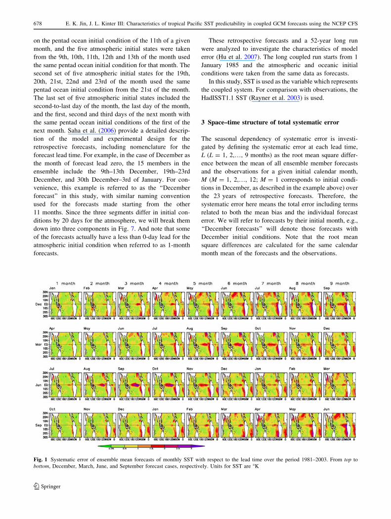
Fig. 1 Systematic error of ensemble mean forecasts of monthly SST with respect to the lead time over the period 1981–2003. From top to

bottom, December, March, June, and September forecast cases, respectively. Units for SST are �K

678 E. K. Jin, J. L. Kinter III: Characteristics of tropical Pacific SST predictability in coupled GCM forecasts using the NCEP CFS

123

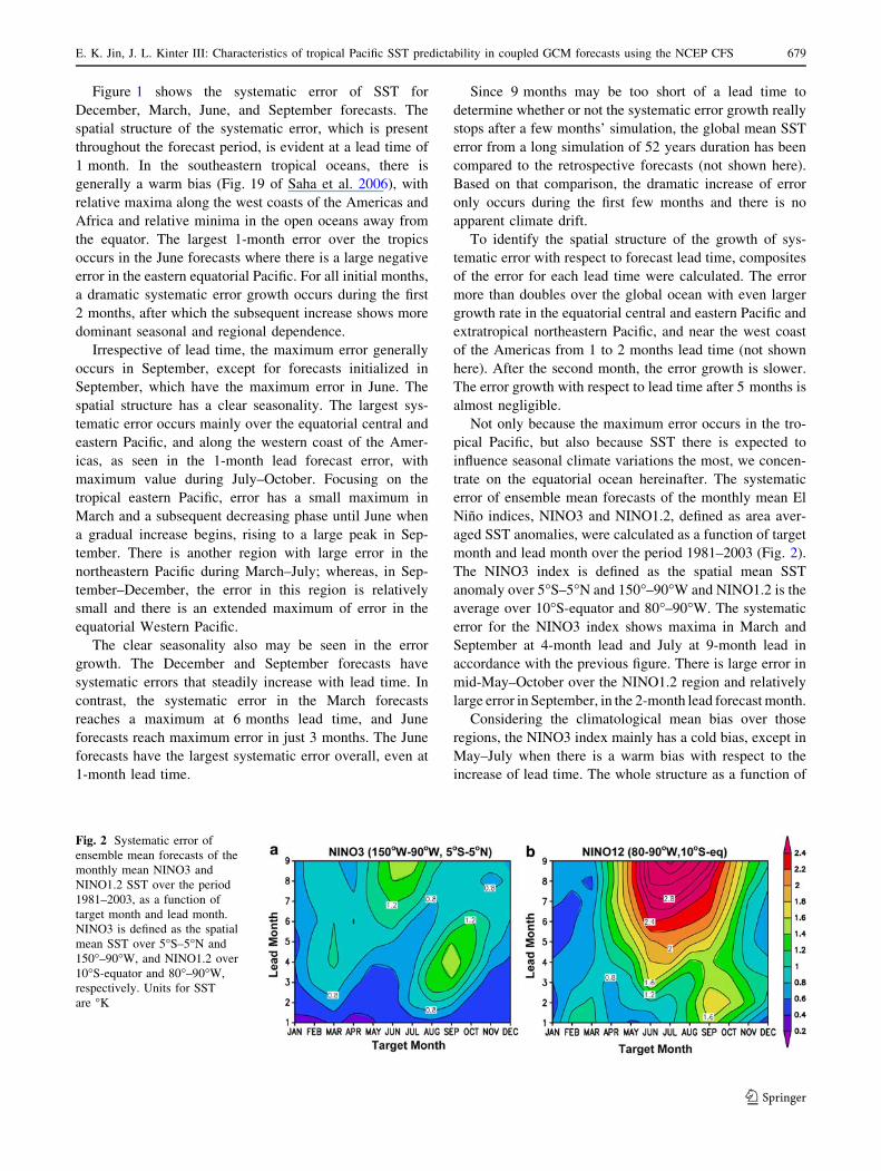
Figure 1 shows the systematic error of SST for

December, March, June, and September forecasts. The

spatial structure of the systematic error, which is present

throughout the forecast period, is evident at a lead time of

1 month. In the southeastern tropical oceans, there is

generally a warm bias (Fig. 19 of Saha et al. 2006), with

relative maxima along the west coasts of the Americas and

Africa and relative minima in the open oceans away from

the equator. The largest 1-month error over the tropics

occurs in the June forecasts where there is a large negative

error in the eastern equatorial Pacific. For all initial months,

a dramatic systematic error growth occurs during the first

2 months, after which the subsequent increase shows more

dominant seasonal and regional dependence.

Irrespective of lead time, the maximum error generally

occurs in September, except for forecasts initialized in

September, which have the maximum error in June. The

spatial structure has a clear seasonality. The largest sys-

tematic error occurs mainly over the equatorial central and

eastern Pacific, and along the western coast of the Amer-

icas, as seen in the 1-month lead forecast error, with

maximum value during July–October. Focusing on the

tropical eastern Pacific, error has a small maximum in

March and a subsequent decreasing phase until June when

a gradual increase begins, rising to a large peak in Sep-

tember. There is another region with large error in the

northeastern Pacific during March–July; whereas, in Sep-

tember–December, the error in this region is relatively

small and there is an extended maximum of error in the

equatorial Western Pacific.

The clear seasonality also may be seen in the error

growth. The December and September forecasts have

systematic errors that steadily increase with lead time. In

contrast, the systematic error in the March forecasts

reaches a maximum at 6 months lead time, and June

forecasts reach maximum error in just 3 months. The June

forecasts have the largest systematic error overall, even at

1-month lead time.

Since 9 months may be too short of a lead time to

determine whether or not the systematic error growth really

stops after a few months’ simulation, the global mean SST

error from a long simulation of 52 years duration has been

compared to the retrospective forecasts (not shown here).

Based on that comparison, the dramatic increase of error

only occurs during the first few months and there is no

apparent climate drift.

To identify the spatial structure of the growth of sys-

tematic error with respect to forecast lead time, composites

of the error for each lead time were calculated. The error

more than doubles over the global ocean with even larger

growth rate in the equatorial central and eastern Pacific and

extratropical northeastern Pacific, and near the west coast

of the Americas from 1 to 2 months lead time (not shown

here). After the second month, the error growth is slower.

The error growth with respect to lead time after 5 months is

almost negligible.

Not only because the maximum error occurs in the tro-

pical Pacific, but also because SST there is expected to

influence seasonal climate variations the most, we concen-

trate on the equatorial ocean hereinafter. The systematic

error of ensemble mean forecasts of the monthly mean El

Nino indices, NINO3 and NINO1.2, defined as area aver-

aged SST anomalies, were calculated as a function of target

month and lead month over the period 1981–2003 (Fig. 2).

The NINO3 index is defined as the spatial mean SST

anomaly over 5�S–5�N and 150�–90�W and NINO1.2 is the

average over 10�S-equator and 80�–90�W. The systematic

error for the NINO3 index shows maxima in March and

September at 4-month lead and July at 9-month lead in

accordance with the previous figure. There is large error in

mid-May–October over the NINO1.2 region and relatively

large error in September, in the 2-month lead forecast month.

Considering the climatological mean bias over those

regions, the NINO3 index mainly has a cold bias, except in

May–July when there is a warm bias with respect to the

increase of lead time. The whole structure as a function of

Fig. 2 Systematic error of

ensemble mean forecasts of the

monthly mean NINO3 and

NINO1.2 SST over the period

1981–2003, as a function of

target month and lead month.

NINO3 is defined as the spatial

mean SST over 5�S–5�N and

150�–90�W, and NINO1.2 over

10�S-equator and 80�–90�W,

respectively. Units for SST

are �K

E. K. Jin, J. L. Kinter III: Characteristics of tropical Pacific SST predictability in coupled GCM forecasts using the NCEP CFS 679

123

target month and lead month is well matched with that of

systematic error (not shown here). The large warm bias

over the NINO1.2 region also shows a clear resemblance to

the structure of systematic error. This means that many

aspects of the systematic error reflect the seasonality and

growth of the climatological mean bias.

The facts that the CFS mean bias exhibits its typical

spatial structure early in the forecast and that the systematic

error is tightly linked to the annual cycle both in terms of

magnitude and growth rate strongly suggest that a simple

flux correction applied to the SST in the course of a fore-

cast could substantially reduce the forecast error. This

possibility is left for a future study.

4 ENSO phase-locking and the seasonal dependence

of RMS error

As shown in Sect. 3, the mean CFS error is very systematic

in terms of its spatial structure and seasonality, so it can be

removed a posteriori. The average of all ensemble mean

forecasts for a given calendar month was subtracted from

all the forecasts for that particular initial month. In this

way, the mean bias is a function of lead time. And the

mean annual cycle of monthly means was subtracted from

the observations, and the root-mean-squared (RMS) error

was computed from the remainder. Hereafter, RMS will

refer to the root mean square error after the monthly mean

systematic error has been removed.

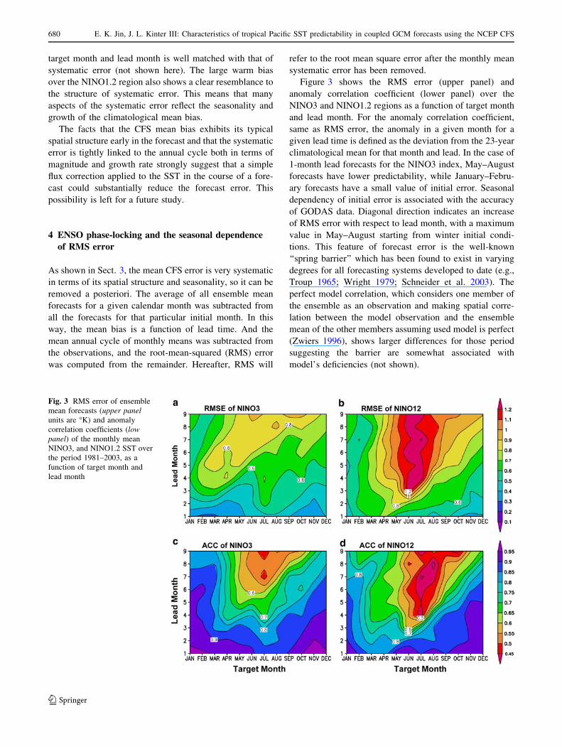
Figure 3 shows the RMS error (upper panel) and

anomaly correlation coefficient (lower panel) over the

NINO3 and NINO1.2 regions as a function of target month

and lead month. For the anomaly correlation coefficient,

same as RMS error, the anomaly in a given month for a

given lead time is defined as the deviation from the 23-year

climatological mean for that month and lead. In the case of

1-month lead forecasts for the NINO3 index, May–August

forecasts have lower predictability, while January–Febru-

ary forecasts have a small value of initial error. Seasonal

dependency of initial error is associated with the accuracy

of GODAS data. Diagonal direction indicates an increase

of RMS error with respect to lead month, with a maximum

value in May–August starting from winter initial condi-

tions. This feature of forecast error is the well-known

‘‘spring barrier’’ which has been found to exist in varying

degrees for all forecasting systems developed to date (e.g.,

Troup 1965; Wright 1979; Schneider et al. 2003). The

perfect model correlation, which considers one member of

the ensemble as an observation and making spatial corre-

lation between the model observation and the ensemble

mean of the other members assuming used model is perfect

(Zwiers 1996), shows larger differences for those period

suggesting the barrier are somewhat associated with

model’s deficiencies (not shown).

Fig. 3 RMS error of ensemble

mean forecasts (upper panelunits are �K) and anomaly

correlation coefficients (lowpanel) of the monthly mean

NINO3, and NINO1.2 SST over

the period 1981–2003, as a

function of target month and

lead month

680 E. K. Jin, J. L. Kinter III: Characteristics of tropical Pacific SST predictability in coupled GCM forecasts using the NCEP CFS

123

In contrast to the NINO3 index, the NINO1.2 index has

large initial error for February–April forecasts. In addition,

the RMS error is dominated by the seasonality with a large

maximum value in May–August and a relatively weak

dependence on lead time. Since the systematic error has a

strong seasonal dependence during June–September in the

eastern and southeastern Pacific (Fig. 1), it is apparent that

the systematic and RMS errors are phase-locked in the

NINO1.2 region.

To prevent being misled by the variation of monthly vari-

ance, the root-mean-square error normalized by the respective

calendar month standard deviation (rmsn) is calculated as a

function of target month and lead month and compared with

the RMS error in Fig. 4 (not shown). As a result, the main

features of the structure and seasonal dependency are identical

except for a small change of amplitude.

Anomaly correlation coefficients also support this sea-

sonal dependency of error growth. The forecast error

growth over the tropical Pacific shows clear seasonal

characteristics. This marked decay in skill during spring

(the ‘‘spring barrier’’), followed sometimes by a recovery

of skill in autumn and winter, is common to most models

(e.g., Webster and Yang 1992; Latif et al. 1994; Clarke and

Van Gorder 1999). Several processes are the plausible

candidate causes of the seasonal dependence, based on

previous studies. These include the intrinsic nature of SST,

the seasonal change of SST persistence associated with the

interannual variability of SST and ENSO phase locked to

the seasonal cycle (Zebiak and Cane 1987; Battisti 1988;

Goswami and Shukla 1991; Xue et al. 1994); the signal-

to-noise ratio of SST (DeWitt 2005); and the change of

relationship between upper-ocean heat content and SST

with respect to season (Kleeman 1993; Galanti et al. 2002;

McPhaden 2003). Based on the model, the seasonal accu-

racy of initialization and model error to simulate the ENSO

can influence on the seasonal dependency of skill.

In this study, ENSO phase-locking to the seasonal cycle

is considered to explain the spring barrier shown in this

JanuaryAprilJulyOctober

El Nino GrowthLa Nina GrowthEl Nino DecayLa Nina DecayNormal

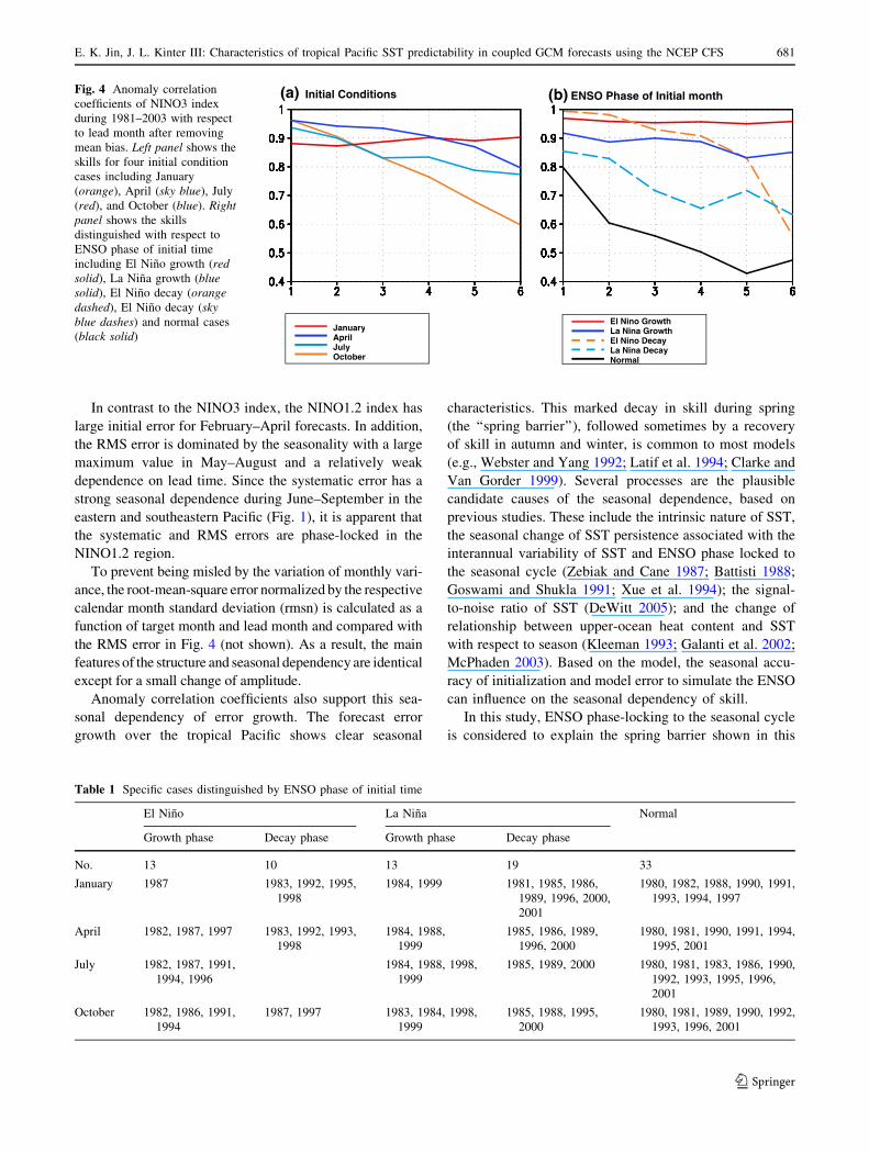
Initial Conditions(a) (b) ENSO Phase of Initial monthFig. 4 Anomaly correlation

coefficients of NINO3 index

during 1981–2003 with respect

to lead month after removing

mean bias. Left panel shows the

skills for four initial condition

cases including January

(orange), April (sky blue), July

(red), and October (blue). Rightpanel shows the skills

distinguished with respect to

ENSO phase of initial time

including El Nino growth (redsolid), La Nina growth (bluesolid), El Nino decay (orangedashed), El Nino decay (skyblue dashes) and normal cases

(black solid)

Table 1 Specific cases distinguished by ENSO phase of initial time

El Nino La Nina Normal

Growth phase Decay phase Growth phase Decay phase

No. 13 10 13 19 33

January 1987 1983, 1992, 1995,

1998

1984, 1999 1981, 1985, 1986,

1989, 1996, 2000,

2001

1980, 1982, 1988, 1990, 1991,

1993, 1994, 1997

April 1982, 1987, 1997 1983, 1992, 1993,

1998

1984, 1988,

1999

1985, 1986, 1989,

1996, 2000

1980, 1981, 1990, 1991, 1994,

1995, 2001

July 1982, 1987, 1991,

1994, 1996

1984, 1988, 1998,

1999

1985, 1989, 2000 1980, 1981, 1983, 1986, 1990,

1992, 1993, 1995, 1996,

2001

October 1982, 1986, 1991,

1994

1987, 1997 1983, 1984, 1998,

1999

1985, 1988, 1995,

2000

1980, 1981, 1989, 1990, 1992,

1993, 1996, 2001

E. K. Jin, J. L. Kinter III: Characteristics of tropical Pacific SST predictability in coupled GCM forecasts using the NCEP CFS 681

123

model. Figure 4a shows the anomaly correlation coeffi-

cients of the NINO3 index as a function of forecast lead

month for four initial condition cases. The forecast skill

also shows clear seasonality associated with spring barrier,

with a fast drop of skill for January and April initial con-

ditions and moderate change of skill for July and October

initial conditions in the first 6 months.

Furthermore, the ENSO phase at the initial time, based

on the observed monthly NINO3 index, distinguishes the

cases. Using the half of one standard deviation of observed

SST anomalies, which is calculated separately for warm

and cold anomalies to consider the asymmetry, El Nino

growth and decay, La Nina growth and decay, and normal

cases are identified, respectively. Table 1 shows the years

and number of cases in each category selected in this

manner. Due to the ENSO phase locking to the annual

cycle, the growth phase occur frequently in July and

October initial condition cases, and the decaying phase is

more typical in January and April cases. The growth phase

of both warm and cold events is more predictable than the

decay phase (Fig. 4b). Forecasts in the El Nino growth

phase show more sustained skill than in La Nina growth

cases, while cases with a decaying El Nino lose skill faster

than cases of La Nina decay. Normal events are far less

predictable than warm or cold events. Therefore, the fast

drop of skill in January and April cases can be explained

since it includes more decaying phase situations, which

have lower skill than growth phase cases. August and

November forecasts have relatively better skill because

they are less frequently in the decaying phase, due to the

phase locking of ENSO to the annual cycle. The fact that

there is less seasonal dependency of skill for normal cases

(not shown) also supports this result. Jin et al. (2008) have

shown similar conclusion from ten coupled GCM forecast

results. The reason why ENSO growth is more predictable

than decay is less obvious and requires further analysis

(Table 2).

5 Error growth, Lorenz curve, and its implication

on forecast error

Forecast error occurs not only because the initial condition

obtained from the analysis is not perfect, but also because

the model itself has formulation errors. The actual forecast

error defined as the difference between forecast for a given

day started some days earlier and the observation is always

an upper limit for the forecast error. The so-called ‘‘per-

fect-model error’’ is the difference between forecasts

started a short time apart, due to the chaotic dynamics and

the difference in initial conditions. It eliminates consider-

ation of the model’s formulation error. The actual forecast

error results from a combination of model formulation

errors and errors due to chaos. We expect the differences in

forecast error started a few days apart to be less than the

actual forecast error. In this sense, the perfect-model error

might form a lower limit of sorts.

Similarly, the actual forecast error, which gives the

correct skill of forecast, can be considered as the lower

Table 2 Correlation coefficients between observed and simulated NINO3 index for four months including January, April, July, and October

Target month First month Third month Sixth month Ninth month

January 0.96 (December) 0.93 (October) 0.89 (July) 0.81 (April)

April 0.90 (March) 0.83 (January) 0.73 (October) 0.70 (July)

July 0.88 (June) 0.79 (April) 0.58 (January) 0.46 (October)

October 0.95 (September) 0.88 (July) 0.74 (April) 0.55 (January)

Months inside brackets denotes forecast initial month

Forecast Error of Ensemble meanLorenz Curve of Ensemble meanMean Forecast Error of Each MemberMean Lorenz Curve of Each MemberForecast Error of Each MemberLorenz Curve of Each Member

Forecast Lead Month

Fig. 5 Forecast error and Lorenz curve of NINO3 index. Twelve

initial condition cases are averaged with respect to forecast lead

month. Black solid line denotes the forecast error of ensemble mean,

black dashed line is for mean of individual member, and gray dashedlines for individual member. Likewise, red solid line is for the Lorenz

curve of ensemble mean, red dashed line denotes mean of individual

member, and orange dashed lines are for each member, respectively.

Units are �K

682 E. K. Jin, J. L. Kinter III: Characteristics of tropical Pacific SST predictability in coupled GCM forecasts using the NCEP CFS

123

limit of predictability of this coupled system. To assess the

complementary upper limit of predictability, the ‘‘Lorenz

curve’’ suggested in earlier predictability studies is used.

As shown by Goswami and Shukla (1991), the approach

conceived by Lorenz (1969b) for estimating the lower

bound of weather forecast error can also be applied to

climate forecasts. We will refer to that limit as the ‘‘Lorenz

curve’’, which is estimated from monthly mean data by

assembling the locus of the RMS difference between the

1- and 2-months lead forecasts for the first target month,

the RMS difference between the 2- and 3-months lead

forecasts for the second target month, and so on. The

Lorenz curve is one measure of perfect model error growth.

The analysis thus far has been applied solely to ensemble

mean forecasts; however, there is information in the indi-

vidual ensemble members. The sources of error in seasonal

forecasts are mainly the uncertainty in the initial conditions,

model errors, and instabilities of the coupled system. By

comparing the ensemble mean and individual member

cases, the relative importance of model error and initial error

in determining the error growth can be distinguished. The

difference between the upper and lower limits of predict-

ability can be also interpreted as the instability of the system.

Because we have seen that the maximum error variance

is in the eastern tropical Pacific, and for convenience, we

focus on the average of SST anomalies over the NINO3

region in the remainder of this paper. NINO3 is also a good

index of ENSO variability (Barnston et al. 1997). Figure 5

shows the RMS error and Lorenz curve of the NINO3

index as a function of lead time, for all calendar months’

forecasts. The black solid lines indicate ensemble mean

error, dashed lines show the average of individual ensem-

ble members’ RMS errors, and dashed lines denote

individual members. Likewise, the Lorenz curve has been

computed for each ensemble member (matching ensemble

members by the initial date within the initial month) and

for the ensemble mean forecasts of NINO3, as shown in

Fig. 5 with red lines.

In almost all cases, at almost all leads, the ensemble

mean forecast has smaller RMS error than any of the

individual ensemble members. This behavior is found in

many weather and climate prediction systems—multi-

forecast averages have generally lower error variance. This

is a quantitative expression of the conventional wisdom of

forecasters that the consensus forecast is best, on average.

The most striking feature of this figure is that, surprisingly,

the Lorenz curve of the ensemble mean does not grow with

respect to lead month. Focusing on the individual mem-

bers, at month one, 15 different values of error correspond

to the fifteen members of the ensemble, because each one

has been integrated for a slightly different length of time.

After that, the growth rate of forecast error of individual

members is almost the same as the Lorenz curve,

suggesting that this model has very fast error growth due to

instability of system. The behavior of the ensemble mean

and the individual members look contradictory to each

other. However, note that the forecast error growth in

cases, including both ensemble mean and individual

members appears not to be saturated as the lead time

increases to 9 months, although it is not shown here.

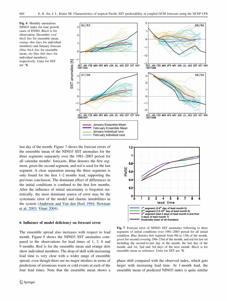
To understand this apparent contradiction, individual

forecast cases from four strong ENSO growth cases were

selected (Fig. 6). The black solid line denotes the observed

NINO3 SST anomalies. The red thick line and the orange

lines are the ensemble mean and individual members of

December initial conditions forecasts and the blue thick

line and the sky-blue lines are January initial conditions

forecasts, respectively. In all cases, the ensemble means of

December and January forecasts are similar to each other,

suggesting that the error is a function of target month

regardless of the initial conditions. This implies that fast

error growth induced by initial conditions has already

saturated, which is consistent with previous results show-

ing fast error growth within 2 months over the tropics.

Even though the ensemble spread is increasing with respect

to lead month in both initial conditions forecast cases, the

ensemble mean error grows similarly, suggesting the strong

regulation of the model’s systematic error by the annual

cycle. For the NINO3 index, this may be a result of the

systematic error of the model ENSO dynamics. That is why

the Lorenz curve is flat, while the differences among

ensemble members show quite a large range, even more

than 4�K sometimes after a few months of model integra-

tion. This also suggests the possibility that ENSO dynamics

in this model appears to be quite wrong.

The flat growth rate of ensemble mean error deceptively

indicates that there is no error growth. However, based on

our analysis of individual cases, it is clear that the initial

error growth is saturated within 2 months in this model.

After this fast error growth saturation induced by initial

errors, the error growth levels off and follows the identical

model error as a function of target month. The fast growth

of the Lorenz curve of individual members results from the

large ensemble spread in CFS due to its instability. Finally

we reach a conclusion analogous to that obtained by

Lorenz’ for weather forecasts, namely that the best way to

improve the 10-day weather forecast is by improving the

first day forecast (Lorenz 1982). We find that the sub-

stantial improvement in ENSO prediction can be obtained

by reducing the first month forecast error.

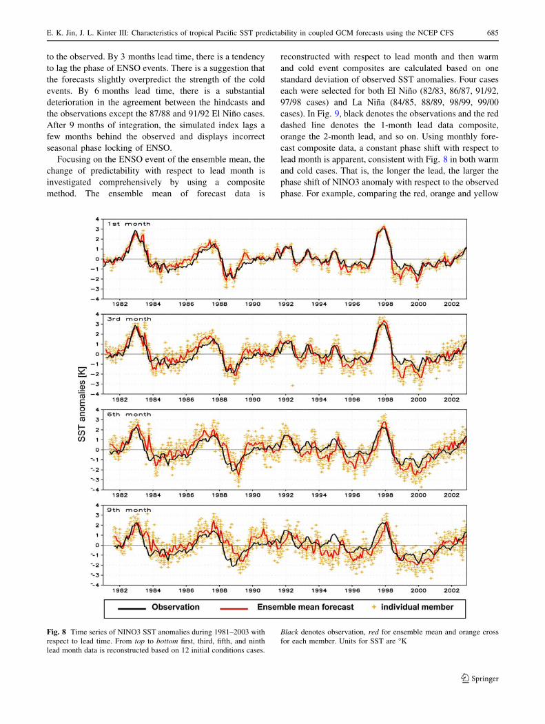
To clarify the effect of initial conditions associated with

lead time, we analyzed the forecast error and its growth for

the three segments of the initial conditions as determined in

the experimental design. The three segments are the fore-

casts initialized near the 11th of the month, those initialized

near the 21st of the month, and those initialized near the

E. K. Jin, J. L. Kinter III: Characteristics of tropical Pacific SST predictability in coupled GCM forecasts using the NCEP CFS 683

123

last day of the month. Figure 7 shows the forecast errors of

the ensemble mean of the NINO3 SST anomalies for the

three segments separately over the 1981–2003 period for

all calendar months’ forecasts. Blue denotes the first seg-

ment, green the second segment, and red is used for the last

segment. A clear separation among the three segments is

only found for the first 1–2 months lead, supporting the

previous conclusion. The dominant effect of differences in

the initial conditions is confined to the first few months.

After the influence of initial uncertainty is forgotten sta-

tistically, the most dominant source of error may be the

systematic error of the model and chaotic instabilities in

the system (Anderson and Van den Dool 1994; Newman

et al. 2003; Vitart 2004).

6 Influence of model deficiency on forecast error

The ensemble spread also increases with respect to lead

month. Figure 8 shows the NINO3 SST anomalies com-

pared to the observations for lead times of 1, 3, 6 and

9 months. Red is for the ensemble mean and orange dots

show individual members. The drop of skill with increasing

lead time is very clear with a wider range of ensemble

spread, even though there are no major misfires in terms of

predictions of erroneous warm or cold events at each of the

four lead times. Note that the ensemble mean shows a

phase shift compared with the observed index, which gets

larger with increasing lead time. At 1-month lead, the

ensemble mean of predicted NINO3 index is quite similar

Fig. 6 Monthly anomalous

NINO3 index for four growth

cases of ENSO. Black is for

observation, December (redthick line for ensemble mean,

orange thin lines for individual

members) and January forecast

(blue thick line for ensemble

mean, sky blue thin lines for

individual members),

respectively. Units for SST

are �K

1st segment (3-9th day of lead month 0)2nd segment (13-19th day of lead month 0)3rd segment (last 2 days of lead month 0 and first 3 days of lead month 1) Ensemble mean of all members

Fig. 7 Forecast error of NINO3 SST anomalies following to three

segments of initial conditions over 1981–2003 period for all initial

condition. Blue denotes first segment form 9th to 13th of the month,

green for second covering 19th–23rd of the month, and red for last set

including the second-to-last day of the month, the last day of the

month, and 1st, 2nd and 3rd days of the next month. Black is for

ensemble mean as reference. Units for SST are �K

684 E. K. Jin, J. L. Kinter III: Characteristics of tropical Pacific SST predictability in coupled GCM forecasts using the NCEP CFS

123

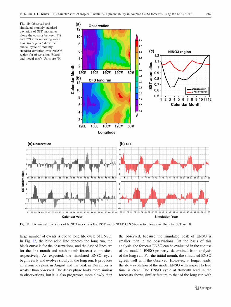
to the observed. By 3 months lead time, there is a tendency

to lag the phase of ENSO events. There is a suggestion that

the forecasts slightly overpredict the strength of the cold

events. By 6 months lead time, there is a substantial

deterioration in the agreement between the hindcasts and

the observations except the 87/88 and 91/92 El Nino cases.

After 9 months of integration, the simulated index lags a

few months behind the observed and displays incorrect

seasonal phase locking of ENSO.

Focusing on the ENSO event of the ensemble mean, the

change of predictability with respect to lead month is

investigated comprehensively by using a composite

method. The ensemble mean of forecast data is

reconstructed with respect to lead month and then warm

and cold event composites are calculated based on one

standard deviation of observed SST anomalies. Four cases

each were selected for both El Nino (82/83, 86/87, 91/92,

97/98 cases) and La Nina (84/85, 88/89, 98/99, 99/00

cases). In Fig. 9, black denotes the observations and the red

dashed line denotes the 1-month lead data composite,

orange the 2-month lead, and so on. Using monthly fore-

cast composite data, a constant phase shift with respect to

lead month is apparent, consistent with Fig. 8 in both warm

and cold cases. That is, the longer the lead, the larger the

phase shift of NINO3 anomaly with respect to the observed

phase. For example, comparing the red, orange and yellow

Fig. 8 Time series of NINO3 SST anomalies during 1981–2003 with

respect to lead time. From top to bottom first, third, fifth, and ninth

lead month data is reconstructed based on 12 initial conditions cases.

Black denotes observation, red for ensemble mean and orange cross

for each member. Units for SST are �K

E. K. Jin, J. L. Kinter III: Characteristics of tropical Pacific SST predictability in coupled GCM forecasts using the NCEP CFS 685

123

curves with the blue, indigo and violet curves, it is apparent

that the former tend to reproduce the observed phase of

NINO3 anomaly quite closely, while the latter are lagged

with respect to the observed. The implication is that the

model tends to persist both warm and cold events too long.

By analyzing four CFS simulations of 32 years each,

Wang et al. (2005) pointed out that the simulated ENSO

events have longer period. Warm events start 3 months

earlier and cold events maintain their strength more in the

model than in observations in the case of NINO3.4 SST

anomalies. Zhang et al. (2007) also showed that CFS

produces an early onset of warm events with longer period:

about 5 years instead of about 4 years in the observations.

Recently, Jin et al. (2008) shows that CFS inherently

generates monotonous type of El Nino different from

observation showing two types of El Nino based on dis-

tinctive spatial pattern of SST anomalies and discharge

mechanism. Simulated El Nino is the midway of two types

and it becomes one of sources of error to reproduce SST

anomalies and associated atmospheric and oceanic

variables.

The problematic features of the simulated ENSO found

in retrospective forecasts may be associated with those of

long runs. In addition, on the premise that the influence of

coupled model errors on actual forecasts is an dominant

factor degrading the predictability after the influence of the

initial conditions fades out as the lead increase, investi-

gating the model capability in long simulations without the

influence of initial conditions is one key to understanding

the behavior of forecast error and identifying possible

means to correct it. In this study, a 52-year long run sim-

ulation is analyzed and compared with forecast data

(K. Pegion, personal communication).

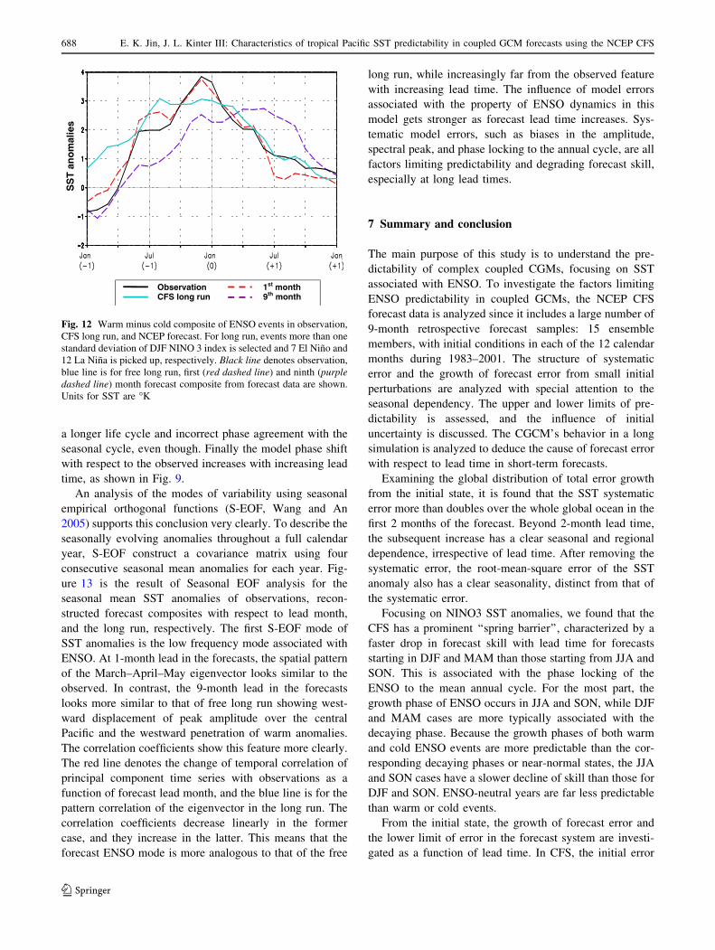
After removing the mean bias by calculating anomalies

as the departures from the climatology of the last 50 years

in the long run, the monthly standard deviation of SST

anomalies over the tropics during the last 50 years is

compared with observations (Fig. 10). Over the eastern and

central Pacific, the observed SST has clear seasonality

showing strong variance in DJF and a weak phase from

February through July. In contrast, the model shows near-

constant high variance over the central and eastern Pacific

even in JJA, unlike the observations. This shows there are

many inconsistencies after even removing the mean bias in

this model. The standard deviation of the NINO3 index

shows this difference very clearly (Fig. 10c). The black

curve is for observations and the red curve is for the long

CFS run. The observed maximum variance is in December

with weak variance in March–July, while the model has

larger variance in March and August unlike the

observations.

The simulated interannual variability of the NINO3

index is also quite different from observed in Fig. 11. The

model has a very regular and long ENSO cycle with a 5- to

6-year period. Associated with this long life cycle, the peak

of ENSO frequently occurs in boreal summer. Therefore,

this model has large error during JJA especially. Based on

the NINO3.4 index, previous studies also show that the

simulated ENSO in the CFS long run has a longer life cycle

with earlier onset and lasts longer, even though the model

reproduces some features of the observed ENSO variability

very well (Wang et al. 2005; Zhang et al. 2007). This

difference may result from the fact that the maximum error

of SST variability occurs over the eastern Pacific, rather

than the central Pacific.

Finally, by computing the warm minus cold composite,

the model ENSO cycle can be compared with observed.

We selected events with more than one standard deviation

of the DJF NINO3 index in the long run. In the 52-year run,

7 El Nino and 12 La Nina events were found. Note that the

Fig. 9 Warm and cold

composite of ENSO events

during 1981–2003. Four

strongest El Nino and La Nina

cases are selected, respectively.

Black solid line denotes

observation, and dashed linesdenotes first to ninth forecast

composite from reconstructed

forecast data with respect to

forecast lead month. Units for

SST are �K

686 E. K. Jin, J. L. Kinter III: Characteristics of tropical Pacific SST predictability in coupled GCM forecasts using the NCEP CFS

123

large number of events is due to long life cycle of ENSO.

In Fig. 12, the blue solid line denotes the long run, the

black curve is for the observations, and the dashed lines are

for the first month and ninth month forecast composites,

respectively. As expected, the simulated ENSO cycle

begins early and evolves slowly in the long run. It produces

an erroneous peak in August and the peak in December is

weaker than observed. The decay phase looks more similar

to observations, but it is also progresses more slowly than

the observed, because the simulated peak of ENSO is

smaller than in the observations. On the basis of this

analysis, the forecast ENSO can be evaluated in the context

of the model’s ENSO property, determined from analysis

of the long run. For the initial month, the simulated ENSO

agrees well with the observed. However, at longer leads,

the slow evolution of the model ENSO with respect to lead

time is clear. The ENSO cycle at 9-month lead in the

forecasts shows similar feature to that of the long run with

Fig. 10 Observed and

simulated monthly standard

deviation of SST anomalies

along the equator between 5�S

and 5�N after removing mean

bias. Right panel show the

annual cycle of monthly

standard deviation over NINO3

region for observation (black)

and model (red). Units are �K

Fig. 11 Interannual time series of NINO3 index in a Had1SST and b NCEP CFS 52-year free long run. Units for SST are �K

E. K. Jin, J. L. Kinter III: Characteristics of tropical Pacific SST predictability in coupled GCM forecasts using the NCEP CFS 687

123

a longer life cycle and incorrect phase agreement with the

seasonal cycle, even though. Finally the model phase shift

with respect to the observed increases with increasing lead

time, as shown in Fig. 9.

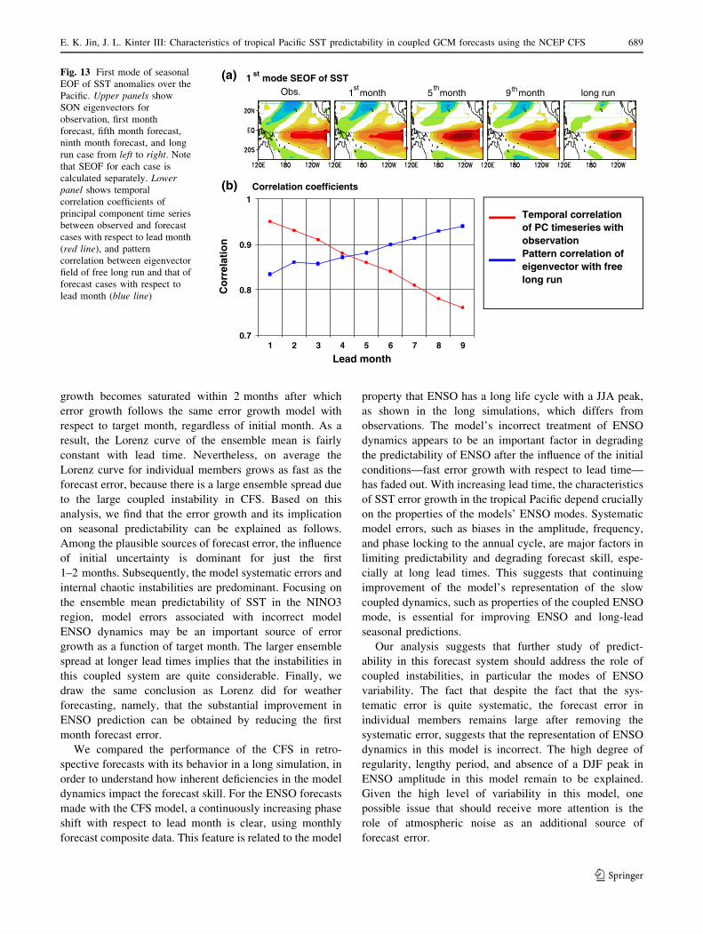
An analysis of the modes of variability using seasonal

empirical orthogonal functions (S-EOF, Wang and An

2005) supports this conclusion very clearly. To describe the

seasonally evolving anomalies throughout a full calendar

year, S-EOF construct a covariance matrix using four

consecutive seasonal mean anomalies for each year. Fig-

ure 13 is the result of Seasonal EOF analysis for the

seasonal mean SST anomalies of observations, recon-

structed forecast composites with respect to lead month,

and the long run, respectively. The first S-EOF mode of

SST anomalies is the low frequency mode associated with

ENSO. At 1-month lead in the forecasts, the spatial pattern

of the March–April–May eigenvector looks similar to the

observed. In contrast, the 9-month lead in the forecasts

looks more similar to that of free long run showing west-

ward displacement of peak amplitude over the central

Pacific and the westward penetration of warm anomalies.

The correlation coefficients show this feature more clearly.

The red line denotes the change of temporal correlation of

principal component time series with observations as a

function of forecast lead month, and the blue line is for the

pattern correlation of the eigenvector in the long run. The

correlation coefficients decrease linearly in the former

case, and they increase in the latter. This means that the

forecast ENSO mode is more analogous to that of the free

long run, while increasingly far from the observed feature

with increasing lead time. The influence of model errors

associated with the property of ENSO dynamics in this

model gets stronger as forecast lead time increases. Sys-

tematic model errors, such as biases in the amplitude,

spectral peak, and phase locking to the annual cycle, are all

factors limiting predictability and degrading forecast skill,

especially at long lead times.

7 Summary and conclusion

The main purpose of this study is to understand the pre-

dictability of complex coupled CGMs, focusing on SST

associated with ENSO. To investigate the factors limiting

ENSO predictability in coupled GCMs, the NCEP CFS

forecast data is analyzed since it includes a large number of

9-month retrospective forecast samples: 15 ensemble

members, with initial conditions in each of the 12 calendar

months during 1983–2001. The structure of systematic

error and the growth of forecast error from small initial

perturbations are analyzed with special attention to the

seasonal dependency. The upper and lower limits of pre-

dictability is assessed, and the influence of initial

uncertainty is discussed. The CGCM’s behavior in a long

simulation is analyzed to deduce the cause of forecast error

with respect to lead time in short-term forecasts.

Examining the global distribution of total error growth

from the initial state, it is found that the SST systematic

error more than doubles over the whole global ocean in the

first 2 months of the forecast. Beyond 2-month lead time,

the subsequent increase has a clear seasonal and regional

dependence, irrespective of lead time. After removing the

systematic error, the root-mean-square error of the SST

anomaly also has a clear seasonality, distinct from that of

the systematic error.

Focusing on NINO3 SST anomalies, we found that the

CFS has a prominent ‘‘spring barrier’’, characterized by a

faster drop in forecast skill with lead time for forecasts

starting in DJF and MAM than those starting from JJA and

SON. This is associated with the phase locking of the

ENSO to the mean annual cycle. For the most part, the

growth phase of ENSO occurs in JJA and SON, while DJF

and MAM cases are more typically associated with the

decaying phase. Because the growth phases of both warm

and cold ENSO events are more predictable than the cor-

responding decaying phases or near-normal states, the JJA

and SON cases have a slower decline of skill than those for

DJF and SON. ENSO-neutral years are far less predictable

than warm or cold events.

From the initial state, the growth of forecast error and

the lower limit of error in the forecast system are investi-

gated as a function of lead time. In CFS, the initial error

ObservationCFS long run

SS

Tan

om

alie

s

1st month9th month

Fig. 12 Warm minus cold composite of ENSO events in observation,

CFS long run, and NCEP forecast. For long run, events more than one

standard deviation of DJF NINO 3 index is selected and 7 El Nino and

12 La Nina is picked up, respectively. Black line denotes observation,

blue line is for free long run, first (red dashed line) and ninth (purpledashed line) month forecast composite from forecast data are shown.

Units for SST are �K

688 E. K. Jin, J. L. Kinter III: Characteristics of tropical Pacific SST predictability in coupled GCM forecasts using the NCEP CFS

123

growth becomes saturated within 2 months after which

error growth follows the same error growth model with

respect to target month, regardless of initial month. As a

result, the Lorenz curve of the ensemble mean is fairly

constant with lead time. Nevertheless, on average the

Lorenz curve for individual members grows as fast as the

forecast error, because there is a large ensemble spread due

to the large coupled instability in CFS. Based on this

analysis, we find that the error growth and its implication

on seasonal predictability can be explained as follows.

Among the plausible sources of forecast error, the influence

of initial uncertainty is dominant for just the first

1–2 months. Subsequently, the model systematic errors and

internal chaotic instabilities are predominant. Focusing on

the ensemble mean predictability of SST in the NINO3

region, model errors associated with incorrect model

ENSO dynamics may be an important source of error

growth as a function of target month. The larger ensemble

spread at longer lead times implies that the instabilities in

this coupled system are quite considerable. Finally, we

draw the same conclusion as Lorenz did for weather

forecasting, namely, that the substantial improvement in

ENSO prediction can be obtained by reducing the first

month forecast error.

We compared the performance of the CFS in retro-

spective forecasts with its behavior in a long simulation, in

order to understand how inherent deficiencies in the model

dynamics impact the forecast skill. For the ENSO forecasts

made with the CFS model, a continuously increasing phase

shift with respect to lead month is clear, using monthly

forecast composite data. This feature is related to the model

property that ENSO has a long life cycle with a JJA peak,

as shown in the long simulations, which differs from

observations. The model’s incorrect treatment of ENSO

dynamics appears to be an important factor in degrading

the predictability of ENSO after the influence of the initial

conditions—fast error growth with respect to lead time—

has faded out. With increasing lead time, the characteristics

of SST error growth in the tropical Pacific depend crucially

on the properties of the models’ ENSO modes. Systematic

model errors, such as biases in the amplitude, frequency,

and phase locking to the annual cycle, are major factors in

limiting predictability and degrading forecast skill, espe-

cially at long lead times. This suggests that continuing

improvement of the model’s representation of the slow

coupled dynamics, such as properties of the coupled ENSO

mode, is essential for improving ENSO and long-lead

seasonal predictions.

Our analysis suggests that further study of predict-

ability in this forecast system should address the role of

coupled instabilities, in particular the modes of ENSO

variability. The fact that despite the fact that the sys-

tematic error is quite systematic, the forecast error in

individual members remains large after removing the

systematic error, suggests that the representation of ENSO

dynamics in this model is incorrect. The high degree of

regularity, lengthy period, and absence of a DJF peak in

ENSO amplitude in this model remain to be explained.

Given the high level of variability in this model, one

possible issue that should receive more attention is the

role of atmospheric noise as an additional source of

forecast error.

1 st mode SEOF of SST

Temporal correlation of PC timeseries with observationPattern correlation of eigenvector with free long run

0.7

0.8

0.9

1

1 2 3 4 5 6 7 8 9

Lead month

Co

rrel

atio

n

Correlation coefficients

Obs.

(a)

(b)

long run1st

month 9thmonth5th

month

Fig. 13 First mode of seasonal

EOF of SST anomalies over the

Pacific. Upper panels show

SON eigenvectors for

observation, first month

forecast, fifth month forecast,

ninth month forecast, and long

run case from left to right. Note

that SEOF for each case is

calculated separately. Lowerpanel shows temporal

correlation coefficients of

principal component time series

between observed and forecast

cases with respect to lead month

(red line), and pattern

correlation between eigenvector

field of free long run and that of

forecast cases with respect to

lead month (blue line)

E. K. Jin, J. L. Kinter III: Characteristics of tropical Pacific SST predictability in coupled GCM forecasts using the NCEP CFS 689

123

Acknowledgments The advice of Jagadish Shukla has been

much appreciated, and also discussions with B. Kirtman, B. Wang,

and J.-Y. Lee. The forecast data was generously provided by the

NCEP Environmental Modeling Center (EMC), long run data was

generously provided by K. Pegion (COLA), and the author is grateful

for these contributions. The first author was supported by the Asian-

Pacific Economic Cooperation Climate Center (APCC) International

Research Project. The second author was supported by grants from

the National Science Foundation (ATM-0332910), the National

Oceanic and Atmospheric Administration (NA04OAR4310034) and

the National Aeronautics and Space Administration (NNG04GG46G).

References

AchutaRao K, Sperber KR (2002) Simulation of the El Nino-Southern

oscillation: results from the coupled model intercomparison

project. Clim Dyn 19:191–209

Anderson JL, van den Dool HM (1994) Skill and return of skill

in dynamic extended-range forecasts. Mon Weather Rev 122:

507–516

Arpe K, Hollingsworth A, Tracton MS, Lorenc AC, Uppala S,

Kallberg P (1985) The response of numerical weather prediction

systems to FGGE level IIbdata—Part II: Forecast verification and

implications for predictability. Q J R Meteorol Soc 111:67–101

Balmaseda MA, Davey MK, Anderson DLT (1995) Decadal

and seasonal dependence of ENSO prediction skill. J Clim

8:2705–2715

Barnston AG, Chelliah M, Goldenberg SB (1997) Documentation of a

highly ENSO-related SST region in the equatorial Pacific. Atmos

Ocean 35:367–383

Battisti DS (1989) On the role of off-equatorial oceanic Rossby waves

during ENSO. J Phys Oceanogr 19:551–560

Battisti DS (1988) Dynamics and thermodynamics of a warming

event in a coupled tropical atmosphere–ocean model. J Atmos

Sci 45:2889–2919

Battisti DS, Hirst AC (1989) Interannual variability in a tropical

atmosphere–ocean model: influence of the basic state, ocean

geometry and nonlinearity. J Atmos Sci 46:1687–1712

Behringer DW et al. (2005) The Global Ocean Data Assimilation

System (GODAS) at NCEP (to be submitted)

Blumenthal MB (1991) Predictability of a coupled ocean–atmosphere

model. J Clim 4:766–784

Cane MA, Zebiak SE, Dolan SC (1986) Experimental forecasts of El

Nino. Nature 321:827–832

Cane M, Zebiak SE (1987) Prediction of El Nino events using a

physical model. In: Cattle H (ed) Atmospheric and oceanic

variability. Royal Meteorological Society Press, Reading, pp

153–182

Charney J, Fleagle RG, Riehl H, Lally VE, Wark DQ (1966) The

feasibility of a global observation and analysis experiment. Bull

Am Meteorol Soc 47:200–220

Chen WY (1989) Estimates of dynamical predictability from NMC

DERF experiments. Mon Weather Rev 117:1227–1236

Clarke AJ, Van Gorder S (1999) The connection between the boreal

spring Southern oscillation persistence barrier and biennial

variability. J Clim 12:610–620

Dalcher A, Kalnay E (1987) Error growth and predictability in

operational ECMWF forecasts. Tellus 39A:474–491

Davey M, Huddleston M, Sperber KR, Braconnot P, Bryan F, Chen

D, Colman RA, Cooper C, Cubasch U, Delecluse P, DeWitt D,

Fairhead L, Flato G, Gordon C, Hogan T, Ji M, Kimoto M, Kitoh

A, Knutson TR, Latif M, Le Treut H, Li T, Manabe S, Mechoso

CR, Meehl GA, Oberhuber J, Power SB, Roeckner E, Terray L,

Vintzileos A, Voss R, Wang B, Washington WM, Yoshikawa I,

Yu J-Y, Yukimoto S, Zebiak SE (2002) A study of coupled

model climatology and variability in tropical ocean regions.

Clim Dyn 18:403–420

Delecluse P, Davey M, Kitamura Y, Philander S, Suarez M,

Bengtsson L (1998) TOGA review paper: coupled general

circulation modeling of the tropical Pacific. J Geophys Res

103:14357–14373

DeWitt DG (2005) Retrospective forecasts of interannual sea surface

temperature anomalies from 1982 to present using a directly

coupled atmosphere–ocean general circulation model. Mon

Weather Rev 133:2972–2995

Galanti E, Tziperman E, Harrison M, Rosati A, Giering R, Sirkes Z

(2002) The equatorial thermocline outcropping—a seasonal

control on the tropical Pacific ocean–atmosphere instability

strength. J Clim 15:2721–2739

Goswami BN, Shukla J (1991) Predictability of the coupled ocean–

atmosphere model. J Clim 4:3–22

Goswami BN, Rajendran K, Sengupta D (1997) Source of seasonality

and scale dependence of predictability in a coupled ocean–

atmosphere model. Mon Weather Rev 125:846–858

Guilyardi E, Gualdi S, Slingo J, Navarra A, Delecluse P, Cole J,

Madec G, Roberts M, Latif M, Terray L (2004) Representing El

Nino in coupled ocean–atmosphere GCMs: the dominant role of

the atmospheric component. J Clim 17:4623–4629

Gutzler DS, Shukla J (1984) Analogs in the wintertime 500 mb height

field. J Atmos Sci 41:177–189

Hu H, Huang B, Pegion K (2007) Leading patterns of the tropical

Atlantic variability in a coupled general circulation model. Clim

Dyn. doi:10.1007/s00382-007-0318-x

Ji M, Kumar A, Leetmaa A (1994) An experimental coupled forecast

system at the National Meteorological Centre. Some early

results. Tellus 46A:398–418

Jin EK, Kinter JL III, Wang B, Park C-K, Kang I-S, Kirtman B, Kug

J-S, Kumar A, Luo J-J, Schemm J, Shukla J, Yamagata T (2008)

Current status of ENSO prediction skill in coupled ocean–

atmosphere models. Clim Dyn (in press)

Kanamitsu M, Ebisuzaki W, Woollen J, Yang S-K, Slingo JJ, Fiorino

M, Potter GL (2002) NCEP-DOE AMIP-II reanalysis (R–2).

Bull Am Meteorol Soc 83:1631–1643

Kirtman BP, Shukla J, Balmaseda M, Graham N, Penland C, Xue Y,

Zebiak S (2002) Current status of ENSO forecast skill: a report to

the climate variability and predictability (CLIVAR) Numerical

Experimentation Group (NEG). CLIVAR Working Group on

seasonal to interannual prediction, 31 pp. Available online at http://

www.cliver.org/publications/wgpreports/wgsip/nino3/report.htm

Kirtman BP (2003) The COLA anomaly coupled model: ensemble

ENSO prediction. Mon Weather Rev 131:2324–2341

Kleeman R (1993) On the dependence of hindcast skill on ocean

thermodynamics in a coupled ocean–atmosphere model. J Clim

6:2012–2033

Latif M, Sterl A, Maier-Reimer E, Junge MM (1993) Climate variability

in a coupled GCM. Part I: The tropical Pacific. J Clim 6:5–21

Latif M et al (2001) ENSIP: the El Nino simulation intercomparison

project. Clim Dyn 18:255–276

Latif M, Barnett TP, Cane MA, Flugel M, Graham NE, von Storch H,

Xu J-S, Zebiak SE (1994) A review of ENSO prediction studies.

Clim Dyn 9:167–179

Lazar A, Vintzileos A, Doblas-reyes FJ, Rogel P, Delecluse P (2005)

Seasonal forecast of tropical climate with coupled ocean–

atmosphere general circulation models: on the respective role

of the atmosphere and the ocean components in the drift of the

surface temperature error. Tellus 57:387–397

Leith CE (1971) Atmospheric predictability and two-dimensional

turbulence. J Atmos Sci 28:148–161

Leith CE, Kraichnan RH (1972) Predictability of turbulent flows.

J Atmos Sci 29:1041–1058

690 E. K. Jin, J. L. Kinter III: Characteristics of tropical Pacific SST predictability in coupled GCM forecasts using the NCEP CFS

123

Leith CE (1978) Objective methods for weather prediction. Annu Rev

Fluid Mech 10:107–128

Lorenz EN (1965) A study of the predictability of a 28-variable

model. Tellus 17:321–333

Lorenz EN (1969a) The predictability of a flow which possesses many

scales of motion. Tellus 21:289–307

Lorenz EN (1969b) Atmospheric predictability as revealed by

naturally occurring analogues. J Atmos Sci 26:636–646

Lorenz EN (1982) Atmospheric predictability experiments with a

large numerical model. Tellus 34:505–513

McPhaden MJ (2003) Tropical Pacific Ocean heat content variations

and ENSO persistence barriers. Geophys Res Lett 30:1480. doi:

10.1029/2003GLO16872

Mechoso CR, Robertson AW, Barth N, Davey MK, Delecluse P, Gent

PR, Ineson S, Kirtman B, Latif M, Le Treut H, Nagai T, Neelin

JD, Philander SGH, Polcher J, Schopf PS, Stockdale T, Suarez

MJ, Terray L, Thual O, Tribbia JJ (1995) The seasonal cycle

over the tropical Pacific in coupled atmosphere–ocean general-

circulation models. Mon Weather Rev 123:2825–2838

Moorthi S, Pan H-L, Caplan P (2001) Changes to the 2001 NCEP

operational MRF/AVN global analysis/forecast system. NWS

Tech. Procedures Bulletin 484, 14 pp. Available online at

http://www.nws.noaa.gov/om/tpb/484.htm

Newman M, Sardeshmukh PD, Winkler CR, Whitaker JS (2003) A

study of subseasonal predictability. Mon Weather Rev

131:1715–1732

Pacanowski RC, Griffies SM (1998) MOM 3.0 manual. NOAA/

GFDL. Available online at http://www.gfdl.noaa.gov/_smg/

MOM/web/guide_parent/guide_parent.html

Rayner NA, Parker DE, Horton EB, Folland CK, Alenxander LV,

Rowell DP, Kent EC, Kaplan A (2003) Global analyses of sea

surface temperature, sea ice, and night marine air temperature

since the late nineteenth century. J Geophys Res 108:4407–4443

Reynolds CA, Webster PJ, Kalnay E (1994) Random error growth in

NMC’s global forecasts. Mon Weather Rev 122:1281–1305

Rosati A, Miyakoda K, Gudgel R (1997) The impact of ocean initial

conditions on ENSO forecasting with a coupled model. Mon

Weather Rev 125:754–772

Saha S, Nadiga S, Thiaw C, Wang J, Wang W, Zhang Q, van den

Dool HM, Pan H-L, Moorthi S, Behringer D, Stokes D, White G,

Lord S, Ebisuzaki W, Peng P, Xie P (2006) The NCEP cliamte

forecast system. J Clim 15:3483–3517

Schneider EK, DeWitt DG, Rosati A, Kirtman BP, Ji L, Tribbia JJ

(2003) Retrospective ENSO forecasts: sensitivity to atmospheric

model and ocean resolution. Mon Weather Rev 131:3038–3060

Schubert SD, Suarez M (1989) Dynamical predictability in a simple

general circulation model: average error growth. J Atmos Sci

46:353–370

Shukla J (1985) Predictability. In: Hoskins BJ, Pearch RP (eds)

Large-scale dynamical processes in the atmosphere. Academic

Press, London, pp 87–122

Shukla J, Kinter JL III (2006) Predictability of seasonal climate

variations: a pedagogical review. In: Palmer T, Hagedorn R (eds)

Predictability of weather and climate. Cambridge University

Press, London, pp 306–341

Simmons AJ, Mureau R, Petroliagis T (1995) Error growth and

estimates of predictability from the ECMWF forecasting system.

Q J R Meteorol Soc 121:1739–1771

Smagorinsky J (1963) General circulation experiments with the

primitive equations. I: The basic experiment. Mon Weather Rev

91:99–164

Torrence C, Webster PJ (1998) The annual cycle of persistence in the

El Nino/Southern oscillation. Q J R Meteorol Soc 124:1985–

2004

Troup AJ (1965) The ‘‘southern oscillation’’. Q J R Meteorol Soc

91:490–506

Vintzileos A, Delecluse P, Sadourny R (1999) On the mechanisms in

a tropical ocean–global atmosphere coupled general circulation

model. Part I: Mean state and the seasonal cycle. Clim Dyn

15:43–62

Vitart F (2004) Monthly forecasting at ECMWF. Mon Weather Rev

132:2761–2779

Wang B, An S-I (2005) A method for detecting season-dependent

modes of climate variability: S-EOF analysis. Geophys Res Lett

32:L15710

Wang W, Saha S, Pan H-L, Nadiga S, White G (2005) Simulation of

ENSO in the new NCEP Coupled Forecast System Model (CFS03).

Mon Weather Rev 133:1574–1593. doi:10.1175/MWR2936.1

Webster PJ, Yang S (1992) Monsoon and ENSO: selectively

interactive systems. Q J R Meteorol Soc 118:877–925

Williamson DL, Kasahara A (1971) Adaptation of meteorological

variables forced by updating. J Atmos Sci 28:1313–1324

Wright PB (1979) Persistence of rainfall anomalies in the central

Pacific. Nature 277:371–374

Xue Y, Cane MA, Zebiak SE, Blumenthal MB (1994) On the

prediction of ENSO: a study with a low-order Markov model.

Tellus 46A:512–528

Yu J-Y (2005) Enhancement of ENSO’s persistence barrier by biennial

variability in a coupled atmosphere–ocean general circulation

model. J Geophys Res 32:L13707. doi:10.1029/2005GL023406

Zebiak SE, Cane MA (1987) A model El Nino-Southern oscillation.

Mon Weather Rev 115:2262–2278

Zwiers FW (1996) Interannual variability and predictability in an

ensemble of AMIP climate simulations conducted with the CCC

GCM2. Clim Dyn 12:825–848

Zhang Q, Kumar A, Xue Y, Wang W, Jin F-F (2007) Analysis of the

ENSO Cycle in NCEP Coupled Forecast Model. J Clim

20:1265–1284

E. K. Jin, J. L. Kinter III: Characteristics of tropical Pacific SST predictability in coupled GCM forecasts using the NCEP CFS 691

123