Simulation of low clouds in the Southeast Pacific by the NCEP GFS: sensitivity to vertical mixing

Atmos. Chem. Phys., 10, 12261–12272, 2010www.atmos-chem-phys.net/10/12261/2010/doi:10.5194/acp-10-12261-2010© Author(s) 2010. CC Attribution 3.0 License.

AtmosphericChemistry

and Physics

Simulation of low clouds in the Southeast Pacific by the NCEP GFS:sensitivity to vertical mixing

R. Sun1, S. Moorthi2, H. Xiao3, and C. R. Mechoso3

1UCAR/Environmental Modeling Center/NCEP/NOAA, Rm 209, 5200 Auth Rd., Camp Springs, MD, 20746, USA2Environmental Modeling Center/NCEP/NOAA, Rm 209, 5200 Auth Rd., Camp Springs, MD, 20746, USA3Department of Atmospheric and Oceanic Sciences University of California, Los Angeles, Los Angeles, California, USA

Received: 22 July 2010 – Published in Atmos. Chem. Phys. Discuss.: 4 August 2010Revised: 22 November 2010 – Accepted: 15 December 2010 – Published: 23 December 2010

Abstract. The NCEP Global Forecast System (GFS) modelhas an important systematic error shared by many other mod-els: stratocumuli are missed over the subtropical easternoceans. It is shown that this error can be alleviated in theGFS by introducing a consideration of the low-level inver-sion and making two modifications in the model’s represen-tation of vertical mixing. The modifications consist of (a)the elimination of background vertical diffusion above theinversion and (b) the incorporation of a stability parameterbased on the cloud-top entrainment instability (CTEI) crite-rion, which limits the strength of shallow convective mixingacross the inversion. A control simulation and three experi-ments are performed in order to examine both the individualand combined effects of modifications on the generation ofthe stratocumulus clouds. Individually, both modificationsresult in enhanced cloudiness in the Southeast Pacific (SEP)region, although the cloudiness is still low compared to theISCCP climatology. If the modifications are applied together,however, the total cloudiness produced in the southeast Pa-cific has realistic values. This nonlinearity arises as the ef-fects of both modifications reinforce each other in reducingthe leakage of moisture across the inversion. Increased mois-ture trapped below the inversion than in the control run with-out modifications leads to an increase in cloud amount andcloud-top radiative cooling. Then a positive feedback due toenhanced turbulent mixing in the planetary boundary layerby cloud-top radiative cooling leads to and maintains the stra-tocumulus cover. Although the amount of total cloudinessobtained with both modifications has realistic values, the rel-ative contributions of low, middle, and high layers tend to

Correspondence to:R. Sun([email protected])

differ from the observations. These results demonstrate thatit is possible to simulate realistic marine boundary cloudsin large-scale models by implementing direct and physicallybased improvements in the model parameterizations.

1 Introduction

The climatology of the tropical and subtropical Pacific Oceansouth of the Equator is characterized by large east-west gra-dients in sea surface temperature (SST), with values increas-ing from∼20◦C along the South American coast to∼29◦Cin the Western Pacific warm pool. Going west up the SSTgradient, the dominant cloud type changes from stratocu-mulus with high coverage near the coast to shallow cumu-lus with much lower coverage over the central Pacific. Thisevolution of cloud regime occurs in the descending branch ofthe atmospheric Hadley-Walker circulation, with trade windsalong the surface, and a trade wind inversion in the lower tro-posphere that elevates and weakens along the direction ofthe SST gradient. In this broad sense, the Southeast Pa-cific (SEP) climate is a tightly coupled system, in whichpoorly understood interactions develop among clouds, ma-rine boundary layer (MBL) processes, upper ocean dynamicsand thermodynamics, coastal currents and upwelling, large-scale subsidence, regional diurnal circulations, and aerosoleffects.

Interactions between the South American continent andthe atmosphere-ocean system in the SEP are extremely im-portant components of both the regional and global climate.The great height and length of the Andes Cordillera formsa sharp barrier to the zonal flow, resulting in a coastal jet ofstrong, low-level southerly winds parallel to the west coast of

Published by Copernicus Publications on behalf of the European Geosciences Union.

http://creativecommons.org/licenses/by/3.0/

12262 R. Sun et al.: Simulation of low clouds in the Southeast Pacific by the NCEP GFS

South America (Garreaud and Munoz, 2005). This, in turn,drives intense coastal oceanic upwelling, bringing cold, deep,and nutrient/biota rich waters to the surface. As a result, theSST is colder along the Chilean and Peruvian coasts than atany comparable latitude elsewhere in the world. The coldsurface in combination with subsiding warm, dry air aloftis ideal for the formation of marine boundary layer clouds.In the observations, these extend almost 2000 km west fromthe Peruvian Coast and form the world’s largest and mostpersistent subtropical stratocumulus cloud deck (Klein andHartmann, 1993; Kollias et al., 2004).

The existence of this stratus cloud deck has a major im-pact on the earth’s radiation budget (Ma et al. 1996; Gor-don et al. 2000). Difficulties in the prediction of marineboundary layer clouds in climate models significantly con-tribute to uncertainties in the tropical cloud feedback (Bonyand Dufresre, 2005). Most atmosphere-ocean coupled gen-eral circulation models (CGCMs) lack the ability to producerealistic cloud decks in the eastern tropical oceans (Mechosoet al., 1995; Ma et al., 1996, Hannay et al., 2009). The cur-rent and earlier operational versions of the National Centersfor Environmental Prediction (NCEP)’s Global Forecast Sys-tem (GFS) are among the CGCMs that suffer from such prob-lem. Underprediction of stratus results in overestimation ofheat flux into the ocean and may be the primary reason whyocean-atmosphere coupled models show positive SST biasesof several degrees off the coast of Peru (Mechoso et al., 1995;Wang et al., 2005; de Szoeke et al., 2006).

These model difficulties with marine boundary layerclouds in the eastern tropical oceans are evident in the 2003version of the operational GFS, which has been used since2003 as the atmospheric component of the Climate Fore-cast System (CFS) to produce operational climate forecastsat NCEP (Saha et al., 2006). The CFS forecasts have largeerrors in the simulated mean SST, especially along the SouthAmerican coast and in the Pacific “equatorial cold tongue”region. These errors are primarily attributable to the lack ofsufficient stratocumulus that results in an incorrect simula-tion of the surface radiation budget. The CFS, however, ob-tains an ENSO-like interannual variation in the tropical Pa-cific with reasonable temporal and spatial patterns (Wang etal., 2005).

At NCEP, several approaches are being followed to im-prove the representation of cloudiness in the SEP and overthe subtropical oceans in general. The present paper reportson a series of studies aimed at improving the simulation ofstratocumulus in the operational GFS/CFS when running insimulation mode, i.e., for a period long enough to establisha model climatology. We search for simple yet physicallybased revisions of the representation of a low-level inversion– temperature/moisture jumps in the lower atmosphere andtheir control on the depth of shallow convection. The revi-sions described in this paper have been implemented in theCFS reanalysis (CFSR), which shows their beneficial impact(Moorthi et al., 2009).

The text is organized as follows. We start in Sect. 2 by pro-viding a brief description of the operational NCEP/GFS. Sec-tion 3 presents the changes made to the GFS physics to im-prove the simulation of tropical marine stratocumulus. Sec-tion 4 describes the experiments performed with the model inorder to assess the impact of the modifications. Sections 5, 6,and 7 describe and discuss the results from the experiments.Section 8 summarizes the work presented and conclusionsreached.

2 Brief description of the GFS

The 2009 version of the GFS uses a spectral triangular trun-cation of 382 waves (T382) in the horizontal (equivalent toa nearly 35 km Gaussian grid), and a hybrid sigma-pressurefinite differencing system (Sela, 2009) in the vertical with 64layers. The model top layer is at∼0.2 hPa.

This GFS version has undergone significant improve-ments from the version of the NCEP model used for theNCEP/NCAR Reanalysis (Kalnay et al., 1996; Kistler et al.,2001). These include upgrades in the parameterization of so-lar radiation transfer (Hou et al., 1996; Hou et al., 2002),planetary boundary layer (PBL) vertical diffusion (Hong andPan, 1996), Simplified Arakawa-Schubert (SAS) cumulusconvection (Pan and Wu, 1995; Hong and Pan, 1998), andgravity wave drag (Kim and Arakawa, 1995). In addition,cloud condensate is a prognostic variable (Moorthi et al.,2001) with a simple cloud microphysics parameterization(Zhao and Carr, 1997; Sundqvist et al., 1989). Both large-scale condensation and the detrainment of cloud water fromcumulus convection provide sources of cloud condensate.

The fractional cloud cover used in the radiation calcula-tion is diagnostically determined from the predicted cloudcondensate based on the approach of Xu and Randall (1996).The contribution of convection to cloud cover is throughdetrained condensate only; there is no explicit “convectivecloud cover”. The operational GFS also uses the Rapid Ra-diative Transfer Model (RRTM) longwave parameterizationfrom Atmospheric and Environmental Research Inc. (AER,Mlawer et al., 1997) with maximum/random cloud over-lap and a modified version of the National Aeronautics andSpace Administration (NASA) Goddard Space Flight Center(GSFC) shortwave radiation (Hou et al., 2002; Chou et al.,1998) with random overlap. The latter scheme is known tooverestimate shortwave radiation under cloudy conditions.

Ozone is a prognostic variable with a simple parameteri-zation for ozone production and destruction. The model alsoincorporates the four-layer Noah community land-surfacemodel (Ek et al., 2003). In addition to gravity-wave drag, aparameterization of mountain blocking (Alpert, 2004) is in-cluded, following the subgrid-scale orographic drag parame-terization by Lott and Miller (1997).

The shallow convection parameterization follows Tiedtke(1983), and is applied wherever the deep convection

Atmos. Chem. Phys., 10, 12261–12272, 2010 www.atmos-chem-phys.net/10/12261/2010/

R. Sun et al.: Simulation of low clouds in the Southeast Pacific by the NCEP GFS 12263

parameterization is not active. In this scheme, the shallow-convective cloud top is defined as the highest layer below0.7*Ps for which a test parcel from the second model layeris positively buoyant. The cloud base is the Lifting Con-densation Level (LCL) for the same test parcel. Enhancedvertical eddy diffusion is applied to temperature and specifichumidity within this cloud layer; the diffusion coefficientsare prescribed with a maximum value of 5 m2 s−1 near thecloud center and approach zero near the edges.

The PBL scheme in the GFS is based on the Troen andMahrt (1986) paper and was implemented by Hong and Pan(1996). The scheme is a first-order vertical diffusion scheme.The PBL height is diagnostically determined by the bulk-Richardson approach. Once the PBL height is determined,the profile of the coefficient of diffusivity is specified as acubic function of the PBL height. There is also a counter-gradient flux parameterization that is based on the fluxes atthe surface and the convective velocity scale.

3 Modifications of the GFS

The parameterization of shallow convection has an importantinfluence on the simulated formation and/or destruction ofmarine stratocumulus. Wang et al. (2004) found that turningoff the shallow convection parameterization in their regionalmodel simulations dramatically increased the boundary layercloud amount. De Szoeke et al. (2006) examined the effectof shallow convection on the eastern Pacific climate usinga regional ocean-atmosphere model. They found that shal-low convection acts to reduce stratus cloud formation andthat with no shallow convection stratiform cloud fraction in-creases, resulting in an excessive SST cooling.

Strong low-level inversions are expected to limit the verti-cal extent of shallow clouds. In the GFS version we startedwith, however, the existence of a low-level inversion was ig-nored and shallow clouds were allowed to extend from theLCL up to 0.7 Ps . Thus, they could actually extend across theinversion layer irrespective of its strength, leading to its er-roneous weakening in all cases. This process also resulted inexcessive drying and warming of the layers below the inver-sion, where the cloud amount was severely limited. There-fore, as a first step we introduce consideration of the low-level inversion into the shallow convection scheme of theGFS.

A low-level inversion is defined as the region comprisedof model layers below 0.65Ps in which dT /dP (T andP

are temperature and pressure, respectively) satisfies the fol-lowing requirements: (i) is less than 0.0001 K/Pa, and (ii)changes sign at one or two of the layers below. Next, we re-quire the mixing associated with shallow convection to beconfined below the inversion when the inversion is stableenough as measured by a parameter based on the cloud-topentrainment instability (CTEI) concept. This concept hasbeen used in GCMs for several decades in an attempt to rep-

resent a large-scale control on PBL clouds (Deardorff, 1980;Randall, 1980; Suarez et al., 1983). In its original formula-tion, CTEI predicts runaway entrainment and rapid destruc-tion of stratocumulus when the following condition holds,

κ = cp1θe/L1qt > κ0, (1)

wherecp is the specific heat of dry air under constant pres-sure,L is the latent heat of water vaporization,1θe is thejump of equivalent potential temperature, and1qt is thejump of total water mixing ratio across the inversion. Ac-cording to Randall (1980) and Deardorff (1980) an appropri-ate value to be used in the right hand side of (1) isκ0 = 0.23.As pointed out by many authors (e.g., Kuo and Schubert,1988; Moeng, 2000; Stevens et al., 2005; Siems et al., 1990),Eq. (1) only gives the possibility of buoyancy reversals whenentrained air is mixed with cloudy air and cooled by cloudwater evaporation. Clouds may still remain and entrainmentmay not change abruptly because (a) the fraction of densermixtures generated during entrainment mixing forκ largerthanκ0 may be too small to cause instability, and (b) thesedenser mixtures may not directly enhance the intensity of en-training eddies at the cloud top. Other possible responsesto entrainment drying, like enhanced surface moisture fluxor reduced cloud-top radiative cooling, could either refill thecloud gaps or reduce the intensity of entraining eddies. De-spite these caveats, Large Eddy Simulation Models (LES) incases with both well-mixed and decoupled PBL setups haveshown significant anti-correlation between cloud fraction andκ (Moeng 2000; Lock 2009). Forκ large enough (0.6∼0.7),values of cloud fraction are around 0.1∼0.2. This suggeststhat, even though satisfying threshold conditions likeκ > κ0does not lead to the immediate destruction of cloud-toppedboundary layers,κ seems to be a good empirical indicatorof the stability of stratocumulus decks and a transition toshallow cumulus regime is expected for very largeκ. TheLES study by Xiao et al. (2010) also suggests that in a de-coupled boundary layer with active cumulus updrafts,κ is agood measure of the stability of the inversion-capped stra-tocumulus layer. On the basis of the above empirical evi-dence and theoretical arguments, we propose that in models(like the GFS) that are not designed to fully resolve the de-tailed turbulent structure of cloud-topped boundary layers,κ can be used as a physically based large-scale parameterdetermining whether the inversion is unstable enough to al-low large entrainment mixing and consequent destruction ofstratocumulus in the presence of cumulus updrafts. In thisframework we allow mixing associated with shallow convec-tion to extend across the inversion only when Eq. (1) is satis-fied. In this study we choseκ >κ0 = 0.7 following MacVeanand Mason (1990). There are other more sophisticated ver-sions of Eq. (1), which quantitatively take into account theliquid water amount near the cloud top (e.g., Nicholls andTurton, 1986; Lilly, 2002). For our current study, we wantto first establish the effectiveness of the CTEI criteria in con-trolling low cloud amount. Additional dependence on cloud

www.atmos-chem-phys.net/10/12261/2010/ Atmos. Chem. Phys., 10, 12261–12272, 2010


Table 1. List of experiments performed in this study.

CTEI-condition ZEROBD-condition

CONTROL No NoCTEI Yes NoZEROBD No YesCZ Yes Yes

top liquid water amount will be implemented later on with asophisticated shallow convection scheme.

The GFS also includes a background eddy vertical diffu-sion to enhance mixing close to the surface, where the eddydiffusion calculated by the boundary layer parameterizationis considered inadequate. The coefficient of background dif-fusion decreases exponentially with pressure, with the sur-face value set to 1.0 m2 s−1. For the SEP region, particu-larly near the coast of South America, the inversion heightusually is very low due to strong subsidence. Therefore, thebackground vertical diffusion is strong enough to weaken theinversion and allow moisture exchanges with the free atmo-sphere. Since we have a defined inversion height we can nowzero out the background diffusion in the layers above the in-version.

4 Description of the experiments

We performed a total of four sets of GFS experiments usingobserved SSTs (see Table 1). Each set has six two-monthintegrations starting at initial conditions corresponding to00:00 UTC daily from 13 to 18 June 2008. In these exper-iments we used a T126 version of the model and version 2of the Relaxed Arakawa-Schubert (RAS) parameterization ofdeep convection (Moorthi and Suarez, 1992, 1999). The pri-mary focus for the analyses is the ensemble means for July inthe region between the Equator to 40◦ S and 110◦ W–70◦ W,which we will refer to as the SEP in the remainder of thispaper. All the cross-sections used in the following sectionsare along 20◦ S. This is the line VOCALS observation tookplace. In the future we may compare our simulation resultswith VOCALS observations.

1. The CONTROL experiment was done with the opera-tional treatment of shallow convection and backgrounddiffusion as described in Sect. 3.

2. The CTEI experiment is the same as the CONTROL,except that a low-level inversion is defined and the cri-terion for instability expressed by Eq. (1) is used (CTEI-condtion).

3. The ZEROBD experiment is the same as the CON-TROL, except that the background diffusion is set to 0above the inversion (ZEROBD-condition).

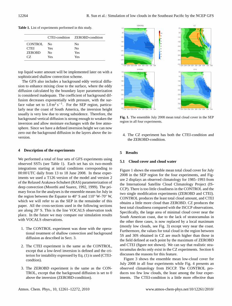
Fig. 1. The ensemble July 2008 mean total cloud cover in the SEPregion in all four experiments.

4. The CZ experiment has both the CTEI-condition andthe ZEROBD-condition.

5 Results

5.1 Cloud cover and cloud water

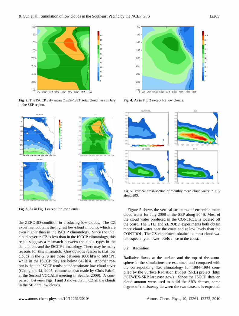
Figure 1 shows the ensemble mean total cloud cover for July2008 in the SEP region for the four experiments, and Fig-ure 2 displays an observed climatology for 1985–1993 fromthe International Satellite Cloud Climatology Project (IS-CCP). There is too little cloudiness in the CONTROL and thetwo single modification experiments (ZEROBD and CTEI).CONTROL produces the least total cloud amount, and CTEIobtains a little more cloud than ZEROBD. CZ produces thebest total cloudiness compared with the ISCCP observations.Specifically, the large area of minimal cloud cover near theSouth American coast, due to the lack of stratocumulus inthe other three cases, is now replaced by a local maximum(mostly low clouds, see Fig. 3) except very near the coast.Furthermore, the values for total cloud in the region between5S and 30S obtained in CZ are much higher than those inthe field defined at each point by the maximum of ZEROBDand CTEI (figure not shown). We can say that realistic stra-tocumulus decks only exist in the CZ experiments. Section 6discusses the reasons for this feature.

Figure 3 shows the ensemble mean low-cloud cover forJuly 2008 in all four experiments while Fig. 4 presents anobserved climatology from ISCCP. The CONTROL pro-duces too few low clouds, the least among the four exper-iments. The CTEI-condition is a little more effective than



Fig. 2. The ISCCP July mean (1985–1993) total cloudiness in Julyin the SEP region.

Fig. 3. As in Fig. 1 except for low clouds.

the ZEROBD-condition in producing low clouds. The CZexperiment obtains the highest low-cloud amounts, which areeven higher than in the ISCCP climatology. Since the totalcloud cover in CZ is less than in the ISCCP climatology, thisresult suggests a mismatch between the cloud types in thesimulations and the ISCCP climatology. There may be manyreasons for this mismatch. One obvious reason is that lowclouds in the GFS are those between 1000 hPa to 680 hPa,while in the ISCCP they are below 642 hPa. Another rea-son is that the ISCCP tends to underestimate low-cloud cover(Chang and Li, 2005; comments also made by Chris Fairallat the Second VOCALS meeting in Seattle, 2009). A com-parison between Figs. 1 and 3 shows that in CZ all the cloudsin the SEP are low clouds.

Fig. 4. As in Fig. 2 except for low clouds.

Fig. 5. Vertical cross-section of monthly mean cloud water in Julyalong 20S.

Figure 5 shows the vertical structures of ensemble meancloud water for July 2008 in the SEP along 20◦ S. Most ofthe cloud water produced in the CONTROL is located offthe coast. The CTEI and ZEROBD experiments both obtainmore cloud water near the coast and at low levels than theCONTROL. The CZ experiment obtains the most cloud wa-ter, especially at lower levels close to the coast.

5.2 Radiation

Radiative fluxes at the surface and the top of the atmo-sphere in the simulations are examined and compared withthe corresponding flux climatology for 1984–1994 com-piled by the Surface Radiation Budget (SRB) project (http://GEWEX-SRB.larc.nasa.gov/). Since the ISCCP data oncloud amount were used to build the SRB dataset, somedegree of consistency between the two datasets is expected.


http://GEWEX-SRB.larc.nasa.gov/

http://GEWEX-SRB.larc.nasa.gov/


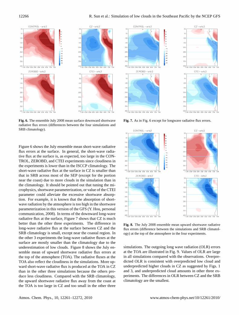
Fig. 6. The ensemble July 2008 mean surface downward shortwaveradiative flux errors (differences between the four simulations andSRB climatology).

Figure 6 shows the July ensemble mean short-wave radiativeflux errors at the surface. In general, the short-wave radia-tive flux at the surface is, as expected, too large in the CON-TROL, ZEROBD, and CTEI experiments since cloudiness inthe experiments is lower than in the ISCCP climatology. Theshort-wave radiative flux at the surface in CZ is smaller thanthat in SRB across most of the SEP (except for the portionnear the coast) due to more clouds in the simulation than inthe climatology. It should be pointed out that tuning the mi-crophysics, shortwave parameterization, or value of the CTEIparameter could alleviate the excessive shortwave absorp-tion. For example, it is known that the absorption of short-wave radiation by the atmosphere is too high in the shortwaveparameterization in this version of the GFS (Y. Hou, personalcommunication, 2008). In terms of the downward long-waveradiative flux at the surface, Figure 7 shows that CZ is muchbetter than the other three experiments. The difference inlong-wave radiative flux at the surface between CZ and theSRB climatology is small, except near the coastal region. Inthe other 3 experiments the long-wave radiative fluxes at thesurface are mostly smaller than the climatology due to theunderestimation of low clouds. Figure 8 shows the July en-semble mean of upward shortwave radiative flux errors atthe top of the atmosphere (TOA). The radiative fluxes at theTOA also reflect the cloudiness in the simulations. More up-ward short-wave radiative flux is produced at the TOA in CZthan in the other three simulations because the others pro-duce less cloudiness. Compared with the SRB climatology,the upward shortwave radiative flux away from the coast atthe TOA is too large in CZ and too small in the other three

Fig. 7. As in Fig. 6 except for longwave radiative flux errors.

Fig. 8. The July 2008 ensemble mean upward shortwave radiativeflux errors (difference between the simulations and SRB climatol-ogy) at the top of the atmosphere in the four experiments.

simulations. The outgoing long wave radiation (OLR) errorsat the TOA are illustrated in Fig. 9. Values of OLR are largein all simulations compared with the observations. Overpre-dicted OLR is consistent with overpredicted low cloud andunderpredicted higher clouds in CZ as suggested by Figs. 1and 3, and underpredicted cloud amounts in other three ex-periments. The differences in OLR between CZ and the SRBclimatology are the smallest.



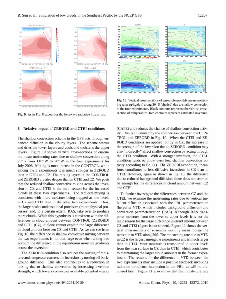
Fig. 9. As in Fig. 8 except for the longwave radiative flux errors.

6 Relative impact of ZEROBD and CTEI-conditions

The shallow convection scheme in the GFS acts through en-hanced diffusion in the cloudy layers. The scheme warmsand dries the lower layers and cools and moistens the upperlayers. Figure 10 shows vertical cross-sections of ensem-ble mean moistening rates due to shallow convection along20◦ S from 110◦ W to 70◦ W in the four experiments forJuly 2008. Mixing is most intense in the CONTROL, whileamong the 3 experiments it is much stronger in ZEROBDthan in CTEI and CZ. The mixing layers in the CONTROLand ZEROBD are also deeper than in CTEI and CZ. We positthat the reduced shallow convective mixing across the inver-sion in CZ and CTEI is the main reason for the increasedclouds in these two experiments. The reduced mixing isconsistent with more moisture being trapped at low levelsin CZ and CTEI than in the other two experiments. Thus,the large-scale condensational processes (microphysical pro-cesses) and, to a certain extent, RAS, take over to producemore clouds. While this hypothesis is consistent with the dif-ferences in cloud amount between CONTROL (ZEROBD)and CTEI (CZ), it alone cannot explain the large differencein cloud amount between CZ and CTEI. As we can see fromFig. 10, the difference in shallow convective mixing betweenthe two experiments is not that large even when taking intoaccount the difference in the equilibrium moisture gradientsacross the inversion.

The ZEROBD-condition also reduces the mixing of mois-ture and temperature across the inversion by turning off back-ground diffusion. This also contributes to a reduction inmixing due to shallow convection by increasing inversionstrength, which lowers convective available potential energy

Fig. 10.Vertical cross-sections of ensemble monthly mean moisten-ing rates (g/kg/day) along 20◦ S (shaded) due to shallow convectionin the four experiments. Black contours represent the vertical cross-section of temperature. Red contours represent estimated inversion.

(CAPE) and reduces the chance of shallow convection activ-ity. This is illustrated by the comparison between the CON-TROL and ZEROBD in Fig. 10. When the CTEI and ZE-ROBD conditions are applied jointly in CZ, the increase inthe strength of the inversion due to ZEROBD-condition mayalso “indirectly” affect shallow convection by acting throughthe CTEI condition. With a stronger inversion, the CTEI-condition tends to allow even less shallow convection ac-tivity according to Eq. (1). The ZEROBD-condition, there-fore, contributes to less diffusive inversions in CZ than inCTEI. However, again as shown in Fig. 10, the differencedue to reduced background diffusion alone does not seem tobe enough for the differences in cloud amount between CZand CTEI.

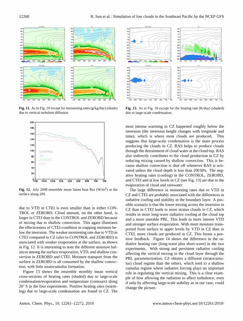
To further investigate the differences between CZ and theCTEI, we examine the moistening rates due to vertical tur-bulent diffusion associated with the PBL parameterization(hereafter VTD, which includes background diffusion) andconvection parameterization (RAS). Although RAS trans-ports moisture from the lower to upper levels it is not themain reason for the large difference in cloud amount betweenCZ and CTEI (figure is not shown). Figure 11 shows the ver-tical cross-sections of ensemble monthly mean moisteningrates due to VTD along 20S. The moistening rate due to VTDin CZ is the largest among the experiments and is much largerthan in CTEI. More moisture is transported to upper levelsfrom the near surface in CZ than in CTEI, which contributesto maintaining the larger cloud amounts in the former exper-iment. The reasons for the difference in VTD between thetwo experiments may include a positive feedback involvingradiation-turbulence interaction in the PBL, as will be dis-cussed later. Figure 11 also shows that the moistening rate



Fig. 11.As in Fig. 10 except for moistening rates (g/kg/day) (shade)due to vertical turbulent diffusion.

Fig. 12. July 2008 ensemble mean latent heat flux (W/m2) at thesurface along 20S

due to VTD in CTEI is even smaller than in either CON-TROL or ZEROBD. Cloud amount, on the other hand, islarger in CTEI than in the CONTROL and ZEROBD becauseof mixing due to shallow convection. This again illustratesthe effectiveness of CTEI-condition in trapping moisture be-low the inversion. The weaker moistening rate due to VTD inCTEI compared to CZ (also to CONTROL and ZEROBD) isassociated with weaker evaporation at the surface, as shownin Fig. 12. It is interesting to note the different moisture bal-ances among the surface evaporation, VTD, and shallow con-vection in ZEROBD and CTEI. Moisture transport from thesurface in ZEROBD is all consumed by the shallow convec-tion, with little stratocumulus formation.

Figure 13 shows the ensemble monthly mean verticalcross-sections of heating rates (shaded) due to large-scalecondensation/evaporation and temperature (contours) along20◦ S in the four experiments. Positive heating rates (warm-ing) due to large-scale condensation are found in CZ. The

Fig. 13. As in Fig. 10 except for the heating rate (K/day) (shaded)due to large-scale condensation.

most intense warming in CZ happened roughly below theinversion (the inversion height changes with longitude andtime), which is where most clouds are produced. Thissuggests that large-scale condensation is the main processproducing the clouds in CZ. RAS helps to produce cloudsthrough the detrainment of cloud water at the cloud top. RASalso indirectly contributes to the cloud production in CZ byreducing mixing caused by shallow convection. This is be-cause shallow convection is shut off whenever RAS is acti-vated unless the cloud depth is less than 200 hPa. The neg-ative heating rates (cooling) in the CONTROL, ZEROBD,and CTEI and at low levels in CZ (see Fig. 13) are due to theevaporation of cloud and rainwater.

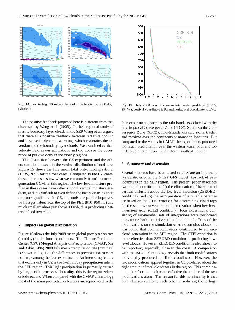
The large difference in moistening rates due to VTD inCZ and CTEI are probably associated with the differences inradiative cooling and stability in the boundary layer. A pos-sible scenario is that the lower mixing across the inversion inCZ than in CTEI leads to more stratus clouds in CZ, whichresults in more long-wave radiative cooling at the cloud topand a more unstable PBL. This leads to more intense VTDand stronger surface evaporation. With more moisture trans-ported from surface to upper levels by VTD in CZ than inCTEI, more clouds are produced in CZ. This forms a pos-itive feedback. Figure 14 shows the difference in the ra-diative heating rate (long-wave plus short-wave) in the twoexperiments. With strong and persistent radiative coolingaffecting the vertical mixing in the cloud layer through thePBL parameterization, CZ obtains a different (stratocumu-lus) cloud regime than the others, which tend to a shallowcumulus regime where radiative forcing plays no importantrole in regulating the vertical mixing. This is a clear exam-ple of how allowing the radiation to affect turbulence, evenif only by affecting large-scale stability as in our case, couldchange the picture.



Fig. 14. As in Fig. 10 except for radiative heating rate (K/day)(shaded).

The positive feedback proposed here is different from thatdiscussed by Wang et al. (2005). In their regional study ofmarine boundary layer clouds in the SEP Wang et al. arguedthat there is a positive feedback between radiative coolingand large-scale dynamic warming, which maintains the in-version and the boundary layer clouds. We examined verticalvelocity field in our simulations and did not see the occur-rence of peak velocity in the cloudy regions.

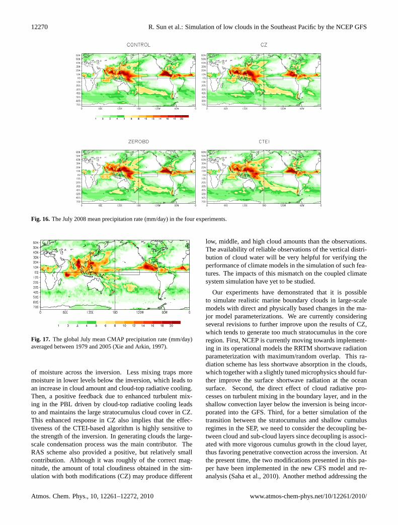
This distinction between the CZ experiment and the oth-ers can also be seen in the vertical distribution of moisture.Figure 15 shows the July mean total water mixing ratio at80◦ W, 20◦ S for the four cases. Compared to the CZ cases,these other cases show what we commonly found in currentgeneration GCMs in this region. The low-level moisture pro-files in these cases have rather smooth vertical moisture gra-dient, and it is difficult to even define the inversion using theirmoisture gradients. In CZ, the moisture profile improves,with larger values near the top of the PBL (910–950 mb) andmuch smaller values just above 900mb, thus producing a bet-ter defined inversion.

7 Impacts on global precipitation

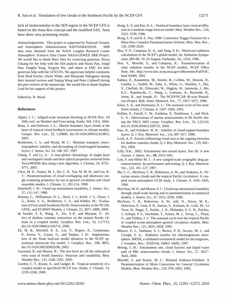
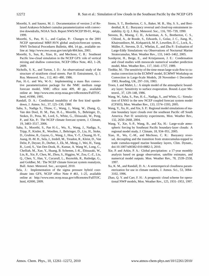
Figure 16 shows the July 2008 mean global precipitation rate(mm/day) in the four experiments. The Climate PredictionCenter (CPC) Merged Analysis of Precipitation (CMAP; Xieand Arkin 1996) 2008 July mean precipitation rate (mm/day)is shown in Fig. 17. The differences in precipitation rate arenot large among the four experiments. An interesting featurethat occurs only in CZ is the 1–2 mm/day precipitation rate inthe SEP region. This light precipitation is primarily causedby large-scale processes. In reality, this is the region wheredrizzle occurs. When compared with the CMAP climatologymost of the main precipitation features are reproduced in the

Fig. 15. July 2008 ensemble mean total water profile at (20◦ S,85◦ W), vertical coordinate is Pa and horizontal coordinate is g/kg.

four experiments, such as the rain bands associated with theIntertropoical Convergence Zone (ITCZ), South Pacific Con-vergence Zone (SPCZ), mid-latitude oceanic storm tracks,and maxima over the continents at monsoon locations. Butcompared to the values in CMAP, the experiments producedtoo much precipitation over the western warm pool and toolittle precipitation over Indian Ocean south of Equator.

8 Summary and discussion

Several methods have been tested to alleviate an importantsystematic error in the NCEP GFS model: the lack of stra-tocumulus in the SEP region. The present paper describestwo model modifications (a) the elimination of backgroundvertical diffusion above the low-level inversion (ZEROBD-condition), and (b) the incorporation of a tunable parame-ter based on the CTEI criterion for determining cloud topsfor the shallow convection parameterization when low-levelinversions exist (CTEI-condition). Four experiments con-sisting of six-member sets of integrations were performedto examine both the individual and combined effects of themodifications on the simulation of stratocumulus clouds. Itwas found that both modifications contributed to enhancecloud generation in the SEP region. The CTEI-condition ismore effective than ZEROBD-condition in producing low-level clouds. However, ZEROBD-condition is also shown tobe important, especially close to the coast. A comparisonwith the ISCCP climatology reveals that both modificationsindividually produced too little cloudiness. However, thetwo modifications applied together in CZ produced about theright amount of total cloudiness in the region. This combina-tion, therefore, is much more effective than either of the twomodifications alone. The reason for this nonlinearity is thatboth changes reinforce each other in reducing the leakage



Fig. 16. The July 2008 mean precipitation rate (mm/day) in the four experiments.

Fig. 17. The global July mean CMAP precipitation rate (mm/day)averaged between 1979 and 2005 (Xie and Arkin, 1997).

of moisture across the inversion. Less mixing traps moremoisture in lower levels below the inversion, which leads toan increase in cloud amount and cloud-top radiative cooling.Then, a positive feedback due to enhanced turbulent mix-ing in the PBL driven by cloud-top radiative cooling leadsto and maintains the large stratocumulus cloud cover in CZ.This enhanced response in CZ also implies that the effec-tiveness of the CTEI-based algorithm is highly sensitive tothe strength of the inversion. In generating clouds the large-scale condensation process was the main contributor. TheRAS scheme also provided a positive, but relatively smallcontribution. Although it was roughly of the correct mag-nitude, the amount of total cloudiness obtained in the sim-ulation with both modifications (CZ) may produce different

low, middle, and high cloud amounts than the observations.The availability of reliable observations of the vertical distri-bution of cloud water will be very helpful for verifying theperformance of climate models in the simulation of such fea-tures. The impacts of this mismatch on the coupled climatesystem simulation have yet to be studied.

Our experiments have demonstrated that it is possibleto simulate realistic marine boundary clouds in large-scalemodels with direct and physically based changes in the ma-jor model parameterizations. We are currently consideringseveral revisions to further improve upon the results of CZ,which tends to generate too much stratocumulus in the coreregion. First, NCEP is currently moving towards implement-ing in its operational models the RRTM shortwave radiationparameterization with maximum/random overlap. This ra-diation scheme has less shortwave absorption in the clouds,which together with a slightly tuned microphysics should fur-ther improve the surface shortwave radiation at the oceansurface. Second, the direct effect of cloud radiative pro-cesses on turbulent mixing in the boundary layer, and in theshallow convection layer below the inversion is being incor-porated into the GFS. Third, for a better simulation of thetransition between the stratocumulus and shallow cumulusregimes in the SEP, we need to consider the decoupling be-tween cloud and sub-cloud layers since decoupling is associ-ated with more vigorous cumulus growth in the cloud layer,thus favoring penetrative convection across the inversion. Atthe present time, the two modifications presented in this pa-per have been implemented in the new CFS model and re-analysis (Saha et al., 2010). Another method addressing the



lack of stratocumulus in the SEP region in the NCEP GFS isbased on the mass-flux concept and the modified SAS. Testshave show very promising results.

Acknowledgements.This project is supported by National Oceanicand Atmospheric Administration NA07OAR4310236. SRBdata were obtained from the NASA Langley Research CenterAtmospheric Sciences Data Center NASA/GEWEX SRB Project.We would like to thank Mary Hart for correcting grammar, HuiyaChuang for her help with the d3d analysis and Hualu Pan, JongilHan, Fanglin Yang, Xingren Wu, and others at EMC for theirgenerous help with the GFS/CFS. We appreciate helpful commentsfrom Brad Ferrier, Glenn White, and Masayuki Nakagawa duringtheir internal reviews and Yuqing Wang and Peter Caldwell duringthe peer reviews of the manuscript. We would like to thank StephenLord for his support of this project.

Edited by: R. Wood

References

Alpert, J. C.: subgrid-scale mountain blocking at NCEP, Proc. Of20th conf. on Weather and Forecasting, Seatle, WA, USA, 2004.

Bony, S. and Dufresre, J.-L.: Marine boundary layer clouds at theheart of tropical cloud feedback uncertainties in climate models,Geopys. Res. Lett., 32, L20806, doi:10.1029/2005GL023851,2005.

Bretherton, C. S., and Wyant, M. C.: Moisture transport, lower-tropospheric stability, and decoupling of cloud-topped boundarylayers, J. Atmos. Sci.,54, 148–167, 1997.

Chang, F. and Li, Z.: A near-global climatology of single-layerand overlapped clouds and their optical properties retrieved fromTerra/MODIS data using a new algorithm, J. Climate, 18, 4752–4771, 2005.

Chou, M. D., Suarez, M. J., Ho, C. H., Yan, M. M. H., and Lee, K.T.: Parameterizations of cloud overlapping and shortwave sin-gle scattering properties for use in general circulation and cloudensemble models, J. Climate, 11, 202-214, 1998.

Deardorff, J. W.: Cloud top entrainment instability, J. Atmos. Sci.,37, 131–147, 1980.

Hannay, C., Williamson, D. L., Hack, J. J., Kiehl, J. T., Olson, J.G., Klein, S. A., Bretherton, C. S., and Kohler, M.: Evalua-tion of Forecasted Southeast Pacific Stratocumulus in the NCAR,GFDL, and ECMWF Models, J. Climate, 22, 2871–2889, 2009.

de Szoeke, S. P., Wang, Y., Xie, S.-P., and Miyama, T.: Ef-fect of shallow cumulus convection on the eastern Pacific cli-mate in a coupled model, Geophys. Res. Lett., 33, L17713,doi:10.1029/2006GL026715, 2006.

Ek, M. B., Mitchell, K. E., Lin, Y., Rogers, E., Grummann,P., Koren, V., Gayno, G., and Tarplay, J. D.: Implementa-tion of the Noah land-use model advances in the NCEP op-erational mesoscale Eta model, J. Geophys. Res., 108, 8851,doi:10.1029/2002JD003296, 2003.

Garreaud, R. and Munoz, R.: The low-level jet off the subtropicalwest coast of South America: Structure and variablility, Mon.Weather Rev., 133, 2246–2261, 2005.

Gordon, C. T., Rosati, A., and Gudgel, R.: Tropical sensitivity of acoupled model to specificed ISCCP low clouds, J. Climate, 13,2239–2260, 2000.

Hong, S.-Y. and Pan, H.-L.: Nonlocal boundary layer vertical diffu-sion in a medium range forecast model. Mon. Weather Rev., 124,2322–2339, 1996.

Hong, S.-Y. and H.-L. Pan, 1998: Convective Trigger Function for aMass-Flux Cumulus Parameterization Scheme, Mon. Wea. Rev.,126, 2599–2620.

Hou, Y.-T., Campana, K. A., and Yang, S. K.: Shortwave radiationcalculations in the NCEP’s global model, Int. Radiation Sympo-sium, IRS-96, 19–24 August, Fairbanks, AL, USA, 1996.

Hou, Y., Moorthi, S., and Campana, K.: Parameterization ofsolar radiation transfer in the NCEP models, NCEP OfficeNote, 441.http://www.emc.ncep.noaa.gov/officenotes/FullTOC.html #2000, 2002.

Kalnay, E., Kanamitsu, M., Kistler, R., Collins, W., Deaven, D.,Gandin, L., Iredell, M., Saha, S., White, G., Woollen, J., Zhu,Y., Chelliah, M., Ebisuzaki, W., Higgins, W., Janowiak, J., Mo,K.C., Ropelewski, C., Wang, J., Leetmaa, A., Reynolds, R.,Jenne, R., and Joseph, D.: The NCEP/NCAR 40-year Reanal-ysis Project, Bull. Amer. Meteorol. Soc., 77, 1057–1072, 1996.

Klein, S. A., and Hartmann, D. L.: The seasonal cycle of low strat-iform clouds, J. Climate, 6, 1587–1606, 1993.

Kollias, P., Fairall, C. W., Zuidema, P., Tomlinson, J., and Wick,G. A.: Observations of marine stratocumulus in SE Pacific dur-ing the PACS 2003 cruise, Geophys. Res. Lett., 31, L22110,doi:10.1029/2004GL020751, 2004.

Kuo, H., and Schubert, W. H.: Stability of cloud-topped boundarylayers. Q. J. Roy. Meteorol. Soc., 114, 887–917, 1988.

Lock, A. P.: Factors influencing cloud area at the capping inversionfor shallow cumulus clouds, Q. J. Roy. Meteorol. Soc., 135, 941–952, 2009.

Lilly, D.K., 2002: Entrainment into mixed layers. Part III: A newclosure.J. Atmos. Sci., 59, 3353-3361.

Lott, F. and Miller M. J.: A new subgrid-scale orographic drag pa-rameterization: Its performance and testing, Q. J. Roy. Meteorol.Soc., 123, 101–127, 1997.

Ma, C.-C., Mechoso, C. R., Robertson, A. W., and Arakawa, A.: Pe-ruvian stratus clouds and the tropical Pacific circulation: A cou-pled ocean-atmosphere GCM study, J. Climate, 9, 1635–1645,1996.

MacVean, M. K. and Mason, P. J.: Cloud-top entrainment instabilitythrough small-scale mixing and its parmeterization in numericalmodels, J. Atmos. Sci., 47, 1012–1030, 1990.

Mechoso, C. R., Robertson, A. W., arth, N., Davey, M. K.,Delecluse, P., Gent, P. R., Ineson, S., Kirtman, B., Latif, M., LeTreut, H., Nagai, T., Neelin., J. D., Philander, S. G. H., Polcher,J., Schope, P. S., Stockdale, T., Suarez, M. J., Terray, L., Thual,O., and Tribbia, J. J.: The seasonal cycle over the tropical Pacificin coupled ocean-atmosphere general circulation models, Mon.Weather Rev., 123, 2825–2838, 1995.

Mlawer, E. J., Taubman, S. J., Brown, P. D., Iacono, M. J., andClough, S. A.: Radiative transfer for inhomogeneous atmo-sphere: RRTM, a validated correlated-K model for the longwave,J. Geophys. Res., 102(D14), 16663–16682, 1997.

Moeng, C.-H.: Entrainment rate, cloud fraction and liquid waterpath of PBL stratocumulus clouds, J. Atmos. Sci., 57, 3627–3643, 2000.

Moorthi, S. and Suarez, M. J.: Relaxed Arakawa-Schubert. AParameterization of Moist Convection for General CirculationModels, Mon. Weather Rev., 120, 978–1002, 1992.


http://www.emc.ncep.noaa.gov/officenotes/FullTOC.html



Moorthi, S. and Saurez, M. J.: Documentation of version 2 of Re-laxed Arakawa-Schubert cumulus parameterization with convec-tive downdrafts, NOAA Tech. Report NWS/NCEP 99-01, 44 pp.,1999.

Moorthi, S., Pan, H. L., and Caplan, P.: Changes to the 2001NCEP operational MRF/AVN global analysis/forecast system,NWS Technical Procedures Bulletin, 484, 14 pp., available on-line at: http://www.nws.noaa.gov/om/tpb/484.htm, 2001.

Moorthi, S., Sun, R., Xiao, H., and Mechoso, C. R.: SoutheastPacific low-cloud simulation in the NCEP GFS: role of verticalmixing and shallow convection, NCEP Office Note, 463, 1–28,2009.

Nicholls, S. K., and Turton, J. D.: An observational study of thestructure of stratiform cloud streets. Part II: Entrainment, Q. J.Roy. Meteorol. Soc., 112, 461–480, 1986.

Pan, H.-L. and Wu, W.-S.: Implementing a mass flux convec-tive parameterization package for the NMC medium rangeforecast model, NMC office note 409, 40 pp., availableonline at: http://www.emc.ncep.noaa.gov/officenotes/FullTOC.html, #1990, 1995.

Randall, D. A.: Conditional instability of the first kind upside-down, J. Atmos. Sci., 37, 125–130, 1980.

Saha, S., Nadiga S., Thiaw, C., Wang, J., Wang, W., Zhang, Q.,Van den Dool, H. M., Pan, H.-L., Moorthi, S., Behringer, D.,Stokes, D., Pena, M., Lord, S., White, G., Ebisuzaki, W., Peng,P., and Xie, P.: The NCEP climate forecast system, J. Climate,19, 3483–3517, 2006.

Saha, S., Moorthi, S., Pan H.-L., Wu, X., Wang, J., Nadiga, S.,Tripp, P., Kistler, R., Woollen, J., Behringer, D., Liu, H., Stoke,D., Grubine, R., Gayno, G., Wang, J., Hou, Y.-T., Chuang, H.-Y.,Juang, H.-M. H., Sela, J., Iredell, M., Treadon, R., Kleist, D., VanDelst, P., Deyser, D., Derber, J., Ek, M., Meng, J., Wei, H., Yang,R., Lord, S., Van Den Dook, H., Kumar, A. Wang W., Long, C.,Chelliah, M., Xue, Y., Huang, B. Schemm, J.-K., Ebisuzaki, W.,Lin, R., Xie, P., Chen, M., Zhou, S., Higgins, W., Zou, C.-Z., Liu,Q., Chen, Y., Han, Y., Cucurull, L., Reynolds, R., Rutledge, G.,and Goldber, M.: The NCEP climate forecast system reanalysis,Bull. Amer. Meteorol. Soc., accepted, 2010.

Sela, J.: Implementation of the sigma pressure hybrid coor-dinate into GFS, NCEP office Note # 461, 1–25, availableonline at: http://www.emc.ncep.noaa.gov/officenotes/FullTOC.html, #2000, 2009.

Siems, S. T., Bretherton, C. S., Baker, M. B., Shy, S. S., and Brei-denthal, R. E.: Buoyancy reversal and cloud-top entrainment in-stability. Q. Q. J. Roy. Meteorol. Soc., 116, 705–739, 1990.

Stevens, B., Moeng, C. H., Ackerman, A. S., Bretherton, C. S.,Chlond, A., de Roode, S., Edwards, J., Golaz, J. C., Jiang, H.,Khairoutdinov, M., Kirkpatrick, M. P., Lewellen, D. C., Lock, A.,Muller, F., Stevens, D. E., Whelan, E., and Zhu P.: Evaluation ofLarge-Eddy Simulations via Observations of Nocturnal MarineStratocumulus, Mon. Weather Rev., 133, 1443–1462, 2005.

Sundqvist, H., Berge, E., and Kristjansson, J. E.: Condensationand cloud studies with mesoscale numerical weather predictionmodel, Mon. Weather Rev., 117, 1641–1757, 1989.

Tiedtke, M.: The sensitivity of the time-mean large-scale flow to cu-mulus convection in the ECMWF model, ECMWF Workshop onConvection in Large-Scale Models, 28 November–1 December1983, Reading, UK, 297–316, 1983.

Troen, I. and Mahrt, L.: A simple model of the atmospheric bound-ary layer; Sensitivity to surface evaporation. Bound.-Layer Me-teorol., 37, 129–148, 1986.

Wang, W., Saha, S., Pan, H.-L., Nadiga, S., and White, G.: Simula-tion of ENSO in the new NCEP coupled forecast system model(CFS03), Mon. Weather Rev., 133, 1574–1593, 2005.

Wang, Y., Xu, H., and Xie, S. P.: Regional model simulations of ma-rine boundary layer clouds over the southeast Pacific off SouthAmerica. Part II: sensitivity experiments, Mon. Weather Rev.,132, 2650–2668, 2004.

Wang, Y., Xie, S.-P., Wang, B., and Xu, H.: Large-scale atmo-spheric forcing by Southeast Pacific boundary-layer clouds: Aregional model study, J. Climate, 18, 934–951, 2005.

Xiao, H., Wu, C.-M., and Mechoso, C. R.: Buoyancy rever-sal, decoupling and the transition from stratocumulus-topped totrade cumulus-topped marine boundary layers, Clim. Dynam.,doi:10.1007/s00382-010-0882-3, 2010.

Xie, P. and Arkin, P. A.: Global precipitation: a 17-year monthlyanalysis based on gauge observation, satellite estimates, andnumerical model outputs. Mon. Weather Rev., 78, 2539–2558,1997.

Xu, K. M., and Randall, D. A.: A semiemperical cloudiness param-eterization for use in climate models, J. Atmos. Sci., 53, 3084–3102, 1996.

Zhao, Q. Y. and Carr, F. H.: A prognostic cloud scheme for opera-tional NWP models, Mon. Weather Rev., 125, 1931–1953, 1997.


http://www.nws.noaa.gov/om/tpb/484.htm





Simulation of low clouds in the Southeast Pacific by the NCEP GFS: sensitivity to vertical mixing

Documents

Transcript of Simulation of low clouds in the Southeast Pacific by the NCEP GFS: sensitivity to vertical mixing