On the Selection of Tags for Tag Clouds

Petros VenetisComputer Science Dept.

Stanford Universityvenetis@cs.stanford.edu

Georgia KoutrikaIBM Almaden Research

Centergkoutri@us.ibm.com

Hector Garcia-MolinaComputer Science Dept.

Stanford Universityhector@cs.stanford.edu

ABSTRACTWe examine the creation of a tag cloud for exploring and under-standing a set of objects (e.g., web pages, documents). In the firstpart of our work, we present a formal system model for reasoningabout tag clouds. We then present metrics that capture the structuralproperties of a tag cloud, and we briefly present a set of tag selec-tion algorithms that are used in current sites (e.g., del.icio.us,Flickr, Technorati) or that have been described in recent work. Inorder to evaluate the results of these algorithms, we devise a novelsynthetic user model. This user model is specifically tailored fortag cloud evaluation and assumes an “ideal” user. We evaluate thealgorithms under this user model, as well as the model itself, usingtwo datasets: CourseRank (a Stanford social tool containing infor-mation about courses) and del.icio.us (a social bookmarkingsite). The results yield insights as to when and why certain selec-tion schemes work best.

Categories and Subject DescriptorsH.1 [Models and Principles]: Miscellaneous; H.3.3 [InformationSearch and Retrieval]: Search process; H.4 [Information Sys-tems Applications]: Miscellaneous

General TermsAlgorithms, Design, Experimentation, Measurement

Keywordstags, tag clouds, tag selection

1. INTRODUCTIONA tag cloud is a visual depiction of text content. Tags are words

found in or associated with the underlying content (e.g., annota-tions) and are typically listed alphabetically and in different coloror font size based on their importance [16]. Tags in the cloud arehyperlinks. The user can click on a tag and see related content.

Tag clouds have been popularized by social sites, such as Flickr,Technorati and del.icio.us, where users annotate shared re-sources using short textual labels, namely tags. In these sites, a tag

Permission to make digital or hard copies of all or part of this work forpersonal or classroom use is granted without fee provided that copies arenot made or distributed for profit or commercial advantage and that copiesbear this notice and the full citation on the first page. To copy otherwise, torepublish, to post on servers or to redistribute to lists, requires prior specificpermission and/or a fee.WSDM’11, February 9–12, 2011, Hong Kong, China.Copyright 2011 ACM 978-1-4503-0493-1/11/02 ...$10.00.

cloud typically summarizes a collection of resources by showingthe most popular tags, i.e., the tags that are most often used for de-scribing resources. For example, in Flickr, users share photos. Auser may upload a photograph that was taken at the Golden Gatebridge at San Francisco and annotate it with the tags ‘ca’, ‘califor-nia’, ‘sanfrancisco’ and ‘goldengate’. A search for photos taggedwith ‘california’ would return a list of photos like the previous oneand a tag cloud summarizing these photos, which could containtags such as: ‘sanfrancisco’, ‘ocean’, ‘beach’, ‘water’, ‘sunset’,‘bridge’, ‘pacific’, ‘usa’, ‘nature’, ‘waves’.

Tag clouds have been used in other settings beyond social in-formation sharing sites, including personal and commercial webpages, blogs, and search engines. They are used for summariz-ing web search results [2], results over biomedical databases [9],and results of structured queries [8]. In these scenarios, tags areextracted from the textual content of the results and are weightedbased on their frequencies. For instance, PubCloud generates a tagcloud from words extracted from the abstracts returned by a queryover the biomedical database PubMed [9].

Despite their popularity, little is known about what makes a tagcloud “good” for summarizing and navigating through a particularcollection. What properties should a tag cloud have? For instance,in social sites, tags are typically selected based on their popularityand a predefined number of them (usually ∼35) is shown to theuser [16]. Are these tags a good choice and why? For example,for the earlier query ‘california’, Flickr may return 1,000 photos.If we select the 35 most popular tags for the cloud, there might besome photos in the query results that have not been assigned anyof the selected 35 tags. These would not be “covered” by the tagcloud and hence would be unreachable by the user clicking on tags.On the other hand, if the query returns just 20 photos, then using(any) 35 tags to represent them may be too much, because tags mayoverlap, such as ‘usa’ and ‘us’, or be assigned to just one photo.

Furthermore, how can we evaluate the output of an algorithm thatselects tags to summarize a corpus? In what sense, is a tag cloud“better” than another for the same corpus? How do we comparethe output of different algorithms (e.g., [2, 8, 9])? If a tag selectionapproach works for one setting, will it be appropriate for differ-ent settings? For example, an earlier work has shown that whensummarizing search results over a database, showing the most fre-quent (popular) words found in the results may provide trivial andnot very meaningful groupings that cannot help the searcher locatesomething interesting. For example, if all photos returned for thequery ‘california’ are also tagged with the word ‘usa’, then the lat-ter is not a good candidate summary word.

With all these questions in mind, in this paper, we focus on thetag selection problem for summarizing a set of results generatedby a query. (We are not interested in the actual tag layout seen

835

by the user.) We define a set of metrics that capture the structuralproperties of a tag cloud. For example, we define the coverageof a tag cloud to show which fraction of the underlying content isdescribed by the cloud and how significant that part is.

Based on these metrics, we develop a user satisfaction model inorder to evaluate the quality of a tag cloud for any given query.Our user model is based on the concept of failure probability. Thisprobability reflects the likelihood that a user is unable to satisfy hissearch goal by using the tag cloud.

Using our framework, we provide a quantitative analysis of sev-eral algorithms for tag selection and we study the quality of theiroutput. We also provide guidelines of how an algorithm should bedevised to minimize the probability of failing to satisfy the user’sneed by empirically examining the failure probability against ourdefined metrics.

For the evaluation, we use two real datasets. The first is a setof (web) documents and tags from the social bookmarking sitedel.icio.us. The other is the course database used in Cours-eRank, a social course planning tool we have developed in InfoLabat Stanford [1]. CourseRank displays official university informa-tion and statistics, such as bulletin course descriptions and gradedistributions, as well as unofficial information, such as user ratingsand reviews. As part of the system, we have implemented Course-Cloud [8] that allows students to explore courses with the help oftag clouds. In this case, the cloud contains the most significant orrepresentative terms found within the results of a search for coursesaggregated over all parts that describe a course, such as the title, thecomments, etc.

Contributions. In summary, our contributions are the following:• We present a framework for reasoning about tag clouds (Sec-

tion 2).•We explore algorithms and metrics for generating and evaluat-

ing tag clouds (Sections 3 and 4).• We develop a user model that captures the “usefulness” of a

tag cloud (Section 5). We show (Section 6.5) via a user study thatour model is good for predicting tag clouds humans prefer.•We evaluate (Section 6) tag creation algorithms using our user

model and two real datasets: one from CourseRank, our courseplanning site in Stanford, and one from the social bookmarkingsite del.icio.us.

2. SYSTEM MODELWe consider a set C of objects (e.g., photos, web pages, etc), and

a set T of tags. These tags may be textual labels assigned to theobjects (e.g., tags assigned to photos) or they may be words ex-tracted from the content of the objects (e.g., words found in the textof a web page or in a course description) or pre-existing categorylabels used to classify documents, and so forth. Each object c in Cis associated with a subset of tags from T .

For simplicity, but without loss of generality, we assume that aquery q belongs to T . Given a query q, the set of results is a setCq ⊆ C. We will denote by Tq the set of tags that are associatedwith at least one of the objects of Cq; obviously Tq ⊆ T . We alsodefine the association set Aq(t) of tag t under query q:DEFINITION 1. The association set Aq(t) of a tag t ∈ Tq under

query q is the set of objects in Cq associated with tag t.Observe that Aq(t) ⊆ Cq by definition.

In our work, we will neither delve into how the set Cq of results isgenerated for a query q nor examine how it is actually ranked. Wewill only assume that there is a partial (scoring) function s(t, c) :T × C → [0, 1]. An object c belongs to Cq iff s(q, c) is definedfor the partial function s(·, ·). For a query q, the scoring function

establishes a partial ordering between objects in Cq . For any twoobjects ci, cj ∈ Cq if s(q, ci) > s(q, cj), then ci is ranked higherthan cj ; if s(q, ci) = s(q, cj), then either ci or cj is ranked higher.

We also assume that there is a similarity function between ob-jects. This similarity function sim(·, ·) : C × C → [0, 1], takes asinputs two objects out of our set C and outputs a number between0 and 1. The higher the value of sim(·, ·) is, the more similar thetwo objects are. For example, if we are dealing with documents,the similarity function could be the Jaccard similarity based on thewords found in each document. If the objects are photographs, thesimilarity function could measure the proximity of the places de-picted in the photographs taking into account geo-referenced data.

A tag cloud is a subset S of the tags in Tq for a particular queryq. Its purpose is two-fold: it is used for summarizing the queryresults and helping navigation. Intuitively, one could imagine thata “good” or effective tag cloud should, in some fundamental sense,be representative of the objects in Cq and should help the user findthe information he wants. To help quantify the properties of tagclouds, we define a set of metrics next.

3. METRICSWe first describe some basic quantities used in our definitions.

For a set of objects Cp ⊆ C:• |Cp| is the number of elements in Cp.• |Cp|s,q =

∑c∈Cp s(q, c) is the scored size of the set Cp under

query q. It is the weighted size of set Cp, where the elements have aweight equal to their score under query q given by the scoring func-tion s. The higher the score of an element is, the more it contributesto the sum.• |Cp|1−s,q =

∑c∈Cp {1− s(q, c)} is the (1−s)-scored size of

the set Cp under query q. It is the weighted size of set Cp, where theelements have a weight equal to one minus their score under queryq. Thus, the higher the score of an element is, the less it contributesto the sum.

Given a query q, the set Cq of query results, and the set Tq oftags associated with objects in Cq , we define the following metricson a subset (tag cloud) S of Tq . Note that some of these metrics (orsimpler variations) have been used to evaluate tag clouds or othertype of sets of terms or documents (see Section 7). Our goal here isto lay out the wide spectrum of choices available, using a consistentterminology and in the specific context of tag clouds.Extent of S: The extent ext(S) of S is the cardinality of S, i.e.:

ext(S) = |S| .

Intuitively, the larger the extent of S is, the more (not necessarilydistinct) topics S potentially covers.Coverage of S: Some objects in Cq may not be associated withany tag from S. Then, these objects are not covered by S. Cover-age gives us the fraction of Cq covered by S. When computing thisfraction, we weigh covered objects by their scores, since it is moreimportant to cover the high-ranked objects than the low-ranked ob-jects. Thus, instead of using plain cardinality of sets, we use scoredsized sets, and we define the coverage cov(S) of S as the scoredsize of the objects that are associated with S over the scored size ofthe original set Cq , i.e.:

cov(S) =

∣∣∣∣ ⋃t∈S

Aq(t)

∣∣∣∣s,q

|Cq|s,q.

This metric can take values between 0 and 1. If cov(S) is closeto 0, then S is associated with a few objects of Cq , and/or with

836

objects in Cq that have a very low score. On the contrary, if cov(S)is close to 1, then the set S is associated with many of the objectsin Cq , and/or with objects that have a very high score.EXAMPLE 1. For our examples in this section, we use our Cours-

eRank setting, where users search for courses. Let us assume thatwe will pick one tag for summarizing the query results (i.e., extentis 1,) and the query was ‘history’ (and s(t, c) = 1 for all t and c).Two candidate tags are ‘Roman’ and ‘Ethiopian’. The tag ‘Roman’gives higher coverage than ‘Ethiopian’, since there are many moreRoman history courses at Stanford than Ethiopian ones.Overlap of S: Different tags in S may be associated with the sameobjects in Cq . The overlap metric captures the extent of such redun-dancy. If tags overlap for low-scored objects, then these objects areover-represented in S, so we want to penalize that. On the otherhand, if they overlap on high-scored objects that are more relevantto the given query, it makes sense to give a lower penalty. Thus, wedefine the overlap over(S) of S as the average pairwise (1 − s)-scored size of the intersection of the associated objects of two tagsover the minimum (1− s)-scored size of the two sets:

over(S) = avgt1,t2∈S,t1 6=t2

|Aq(t1) ∩Aq(t2)|1−s,q

mini∈{1,2}

{|Aq(ti)|1−s,q

}

This metric also takes values in the range [0, 1]. If over(S) isclose to 0, then the intersections of the association sets are verysmall or contain highly scored objects. In this case, each tag revealsa “different aspect” of the query results from the other tags. On theother hand, if over(S) is close to 1, the intersections of the pairsof association sets usually contain all the objects of the smallestset of the pairs, or they include a lot of the low-scored objects. Inthese cases, the tags tend to be not very distinctive or they tend tobe biased towards the less important objects in Cq .EXAMPLE 2. Let us assume a query about ‘computer science’

courses and that we want to select two tags to show in the tag cloud.One could choose the tags ‘programming languages’ and ‘compil-ers’ but these obviously overlap to a great degree. On the otherhand, choosing ‘programming languages’ and ‘databases’ may bea better choice since these are clearly different topics (with small ifany overlap) and they can provide a clearer distinction between thecourses in the result set.Cohesiveness of S: Cohesiveness looks at how closely related theobjects in each association set of S are. For this purpose, we usethe similarity function defined between the objects in C. First, wedefine the average (intra)similarity of the association set Aq(t) ofa tag t ∈ S based on the pair-wise similarities of the objects inAq(t):

sim(t) =

∑c1,c2∈Aq(t),c1 6=c2

sim(c1, c2)

|Aq(t)| × (|Aq(t)| − 1)

The cohesiveness coh(S) of S is defined as the average of (in-tra)similarities of the association sets of the tags in S1:

coh(S) = avgt∈S{sim(t)

}Since the similarity function sim yields values in [0, 1], both

sim(t) and coh(S) produce values in the same range. The highercoh(S) is, the more similar the objects in the association sets areto each other. If cohesiveness is low, then some tags will describe1We could also use minimum or other aggregate functions to de-fine cohesiveness given the sim values. We will not examine otheraggregate functions in this work though.

heterogeneous sets of objects that do not share any distinctive fea-tures.EXAMPLE 3. Assume that our query is ‘computer science’ and ourtag cloud will show one tag. We want to compare two extremes:the tag ‘databases’ and the tag ‘engineering’. Courses with both‘computer science’ and ‘databases’ tags are likely to be closelyrelated, while ‘computer science’ and ‘engineering’ courses arelikely to cover a much wider spectrum of topics. Thus, we expectsim(‘databases’) � sim(‘engineering’). In addition, although‘engineering’ may cover more courses than the tag ‘databases’, thevariety of covered courses may make it hard for a user to locate acourse of interest. On the other hand, ‘databases’ courses form acoherent set, and thus if the tag seems interesting to the user and isclicked, it will lead to potentially interesting courses.Relevance of S: Another interesting question is how relevant thetags in S are to the original query q. To answer this question, wetreat each t in S as a query and we consider the set Ct of objects thatthis query returns. The more Ct and Cq overlap, the more relatedt is to q. If Ct ⊆ Cq , then t is practically a sub-category of theoriginal query q. Let us first define the relevance rel(t, q) of a tagt to the original query q as the fraction of results in Ct that alsobelong to Cq , i.e.:

rel(t, q) =|Ct ∩ Cq||Ct|

.

The relevance rel(S) of S is the average relevance of its tags,i.e.:

rel(S) = avgt∈S{rel(t, q)}

rel(S) lies in [0, 1]. The closer it is to 1, the more relevant are thetags of S to the original query q.EXAMPLE 4. Consider the query ‘computer science’ again and

two potential tags for the cloud: ‘theory’ and ‘relational databases’.There are ‘theory’ courses related to ‘computer science’ but manymore are related to other disciplines. Hence, ‘theory’ is not exclu-sively related to ‘computer science’. On the other hand, all courseson ‘relational databases’ are computer science courses, hence thistag is a highly-relevant topic in computer science.Popularity of S: A tag from S is popular in Cq if it is associatedwith many objects in Cq . We define the popularity pop(S) of S asthe fraction of the sum of the popularities of all tags in S over themaximum possible sum of popularities of any |S| tags that are asubset of Tq , i.e.:

pop(S) =

∑t∈S|Aq(t)|

max{t1,...,t|S|}⊆Tq

{|Aq(t1)|+ . . .+

∣∣Aq(t|S|)∣∣}

Independence of S: All objects in the association set of a tag t1may be similar to each other but they may be also similar to the ob-jects in the association set of a second tag t2. In this case, the twotags may have very similar semantics. Thus, we evaluate the sim-ilarity (or non-similarity) of pairs of different association sets fortags in S. We define a metric similar to cohesiveness, but focusedon pairs of association sets.

First, we define the average similarity between two tags t1, t2 ∈S as2:

sim(t1, t2) =

∑c1∈Aq(t1),c2∈Aq(t2)

sim(c1, c2)

|Aq(t1)| × |Aq(t2)|2Note that the sim operator is overloaded.

837

Then, we define the independence ind(S) of S as:

ind(S) = 1−{

avgt1,t2∈S

{sim(t1, t2)

}}ind(S) takes values in [0, 1]. The higher the value of ind(S), themore “independent” different tags are, which means that they referto dissimilar sets of objects. If it is 0, then many tags in S will besynonyms or one may be very related to each other.

EXAMPLE 5. The two tags ‘programming’ and ‘software’ mayidentify different courses (e.g., ‘Introduction to programming’ vs.‘Object-Oriented Software Design’) but these courses are very sim-ilar, hence the two tags are not independent.

Balance of S: To take into account the relative sizes of associationsets, we define the balance bal(S) of S as follows:

bal(S) =minti∈S{|Aq(ti)|}

maxtj∈S{|Aq(tj)|}

By definition, bal(S) takes values in [0, 1]. The closer it is to 1,the more balanced our association sets are.

EXAMPLE 6. Assume we have the query ‘history’, and two candi-date tag clouds: {‘Greek’, ‘Roman’} vs. {‘European’, ‘Ethiopian’}.The tag ‘Ethiopian’ in the second tag cloud points to very fewcourses whereas the tag ‘European’ is quite generic since it pointsto many courses and would require further drilling down in this setof courses. Thus, the second tag cloud is highly imbalanced andhence not very useful. The first tag cloud is more balanced.

4. ALGORITHMSA tag selection algorithm takes as input a set Cq of objects to

be summarized, a set Tq of tags that can be used to describe theseobjects, and generates a tag cloud S ⊆ Tq .

A tag selection algorithm can be single or multi-objective. Asingle-objective algorithm has a single goal in mind, e.g., maxi-mizing popularity of the cloud. A multi-objective algorithm triesto strike a balance among two or more goals, e.g., achieving highpopularity and coverage. Although multi-objective algorithms havebeen proposed (mainly [3]), in this paper we focus on four single-objective algorithms that have been used in practice or that are veryclose to those used. We believe that trends become more apparentwith single-objective algorithms, and hence our focus. Althoughnot reported here, we have studied multi-objective algorithms, andtheir behavior tends to be a combination of simpler algorithms.That is, an algorithm that tries to optimize metrics X and Y per-forms “somewhere between” an algorithm that optimizes just Xand one that optimizes just Y .

The most common algorithm used in social information shar-ing sites is a popularity-based algorithm, described in Section 4.1.A class of algorithms for structured data is described in [8]. Wedescribe two algorithms in this class in Section 4.2. Our fourthalgorithm (Section 4.3) attempts to maximize coverage, using anapproximate solution to the maximum coverage problem. All thesealgorithms take as input the desired number of tags for the cloud,k, i.e., the extent of the tag cloud.

4.1 Popularity algorithm (POP)Showing popular tags in the cloud allows a user to see what other

people are mostly interested in sharing. For a query q and param-eter k, the algorithm POP returns the top-k tags in Tq according totheir |Aq(t)|. Thus, the algorithm maximizes the popularity metricwe defined in Section 3 (giving a value of 1 for this metric).

4.2 Tf-idf based algorithms (TF, WTF)A different approach is to select good quality tags for the cloud

by giving preference to tags that seem very related when comparedagainst the objects in Cq [8]. Given a query q and a scoring functions(·, ·), this approach proceeds as follows.

Algorithm 1: Tf-idf based algorithmInput: Cq , Tq , tfidf(t, c), s : Tq × Cq → [0, 1]Output: S ⊆ Tq/* PQ is a priority queue. */PQ← ∅, S ← ∅;// Compute all the aggregate confidencesforeach t ∈ Tq do

r ← Ct ∩ Cq ;w ← aggregation

c∈r{f (q, t, c)};

PQ.insert(w, t);

// Select the top-k most confident tagswhile (|S| ≥ k) ∧ (PQ.size() > 0) doS ← S ∪ {PQ.top().getTag()};PQ.pop();

return S;

For each tag t ∈ Tq , it builds the set Aq(t). In order to determinewhether t is highly related to the query results and hence it makesa good selection for the tag cloud, the algorithm produces a scorefor t by aggregating the values of a function f(q, t, c) (which willbe explained shortly) over all objects c ∈ Aq(t); this aggregationyields a score w for tag t. The algorithm returns the k tags with thehighest scores. Function f(q, t, c) can have the following forms:• f (q, t, c) = s(t, c), or• f (q, t, c) = s(t, c) · s(q, c).The first form of f(q, t, c) uses the scoring function s to capture

how related tag t and an object c ∈ Aq(t) are. For example, s(t, c)could be a tf-idf scoring function. If t is very related to the objectsin Aq(t), then it is probably a good tag to be used for describingthese objects. The second form of f(q, t, c) weighs the relatednessbetween t and c, s(t, c), by how related object c is to the query q.The intuition is that a tag t is more significant if it is very related toobjects in the query results that are highly related to the query q.

In our experimental study, we evaluate both forms of functionf(q, t, c). Since in our implementation we use as scoring functionthe tf-idf function between tags and objects, we call the first methodtf-idf (TF for short) and the second one weighted tf-idf (WTF). Also,we use summation as our aggregation function over the objects inAq(t) (average is another of the many possibilities).

4.3 Maximum coverage algorithm (COV)The maximum coverage algorithm (COV) attempts to maximize

the coverage of the resulting set of tags S with the restriction that|S| ≤ k. Our problem is a classic maximum coverage problem,cast in our setting of tags: Our universe of elements (objects) is Cq .We are given subsets Aq(t1), Aq(t2), . . . , Aq(tm) and a parameterk, an upper bound of the extent of S. Our goal is to find a set S ofat most k tags that maximizes cov(S). This problem (even withoutweights/scores) is known to be NP-Complete [15].

Even though our problem is NP-Complete, there are good ap-proximations for it [15]. These approximations have a guaranteedapproximation ratio of e

e−1. Our COV algorithm (in Algorithm 2)

uses a greedy heuristic to find a high coverage tag set. It starts withan empty S. Then, at each round, it adds a tag to S from Tq thatcovers the largest number of uncovered objects by that point. Thealgorithm stops after adding k tags to S or when there are no moretags in Tq .

838

Algorithm 2: Max coverage algorithmInput: Cq , Tq , k, s : Tq × Cq → [0, 1]Output: S ⊆ TqV ← ∅,S ← ∅;// Greedily maximize coveragewhile (|S| ≤ k) ∧ (Tq 6= ∅) do

t̂ = argmaxt∈Tq

{|V ∪Aq(t)|} S ← S ∪{t̂}

;

V ← V ∪Aq(t̂);Tq ← Tq − {t̂};

return S;

5. USER MODELA natural question to ask when comparing tag selection algo-

rithms is, which algorithm yields more “useful” clouds? Unfortu-nately, answering this question is very hard. The goal of tag cloudsis to summarize the available data so the user can better understandwhat is at his disposal. A second goal is to help users discover un-expected information of interest, information that is not reachablevia traditional search since the user does not know how to formu-late a precise query. Neither of these goals can be stated precisely.Furthermore, it is hard to ask users to quantify how well a cloudsummarizes what is available, and what users find “interesting” or“unexpected but interesting” varies widely. The variation can bewide and trends are often hard to observe.

Because of these difficulties, we postulate instead an ideal usersatisfaction model. This “ideal” user is satisfied in a very pre-dictable and rational way. For instance, a tag cloud that is cohesiveand relevant will lead him to objects of interest more often than atag cloud that is not cohesive and/or relevant (more details below).

It is important to note that we do not use the ideal model to pre-dict user satisfaction, we only use it to compare tag clouds. Justlike an “average person” does not exist, our ideal user does not ex-ist so his particular satisfaction score (low failure probability as de-fined below) is not important. The scores are only used to compareclouds, e.g., produced by different algorithms. Our experimentalresults in Section 6.5 indeed do show that our model is relativelygood for predicting clouds users prefer.

5.1 Base model: CoverageSay our ideal user has posed a query q, and he is interested in

just one of the objects in Cq , call it g. We assume that Cq is a largeset; if not, the user could just scan the query results and find whathe wants with no need for a tag cloud. We also assume the userdoes not know how to refine q to narrow down his search to g. Ifhe knew in advance precisely what he wanted, he would again notneed the tag cloud.

The tags in the tag cloud S define a set of objects O covered bythe cloud. That is, O is the union of the Aq(t) sets for all t ∈ S.For now, assume there is no overlap between the Aq(t) sets, andassume the score s(q, c) = 1 for all c ∈ Cq (i.e., the content ofeach object is equally relevant to q).

The objects in O may or may not be of more interest to the userthan the objects in Cq−O. For instance, if the tags in S are popularones, and there is a correlation between popularity and what theuser wants, then an object in O may be more likely to be the desiredobject g than the rest. On the other hand, if the user is browsing fortotally unexpected objects, then all objects in Cq may be of equalinterest (will be equally likely to be g).

To capture this range of scenarios, let us assume that each objectin Cq−O has probability p of being the one the user is interested in,

while objects in O have probability r · p, where r ≥ 1. Parameterr captures how correlated the content of the tag cloud is to the userintention. If r = 1, then we have a “discovery” scenario, where allobjects are equally likely to be of interest. The larger r is, the morelikely it is that the object of interest, g, will be in O (which willbe the case for example if popularity of tags is strongly correlatedwith user’s satisfaction).EXAMPLE 7. Say r = 2, Cq has 10 objects, and O has 6 objects.

Since the user is interested in one object, then 6 ·rp+(10−6) ·p =1, so p = 1/16 = 0.0625. With probability (10 − 6) · p = 4/16,the object g will not be reachable through one of the tags in S.We call this 4/16 = 0.25 the failure probability because if theuser only explores by clicking on tags in the cloud, he will not findg. If coverage increases to say 8 objects in O (r is still 2), then8 · rp + (10 − 8) · p = 1, and thus p = 1/18. In this case, thefailure probability has decreased to 2/18 ≈ 0.11. If instead we goback to 6 objects in O but say that the tags have more influence overuser interest and r = 3, then we have 6 · rp+ (10− 6) · p = 1 andp = 1/22, and the probability of failure also decreases to 4/22 ≈0.18. If both r = 3 and O has 8 objects, then p = 1/26 and thefailure probability is 2/26 ≈ 0.08.

As illustrated, our model assigns a probability to each object inCq , representing the likelihood that the object is g. This distributionis first expressed in terms of p, the probability that an object notcovered by the cloud is the one of interest. Then we solve for pknowing that the probabilities must add up to 1. Once we know thedistribution, we can compute our satisfaction metric:DEFINITION 2. The failure probability (F) for a query q is the

probability that the user will not be able to satisfy his search needusing the tag cloud S.

The failure probability is computed by summing up the probabil-ities p that an object not covered by the cloud is the one of interest,over all objects not covered. The model has a single parameter rthat captures how focused the user exploration is. Although verysimple, this initial model already sheds light on how coverage andtag popularity impact user satisfaction.Summary: We assume that overlap is 0 and that s(q, c) = 1 for allc ∈ Cq . Our first model incorporates only coverage. The probabil-ity that an object c ∈

⋃t∈S Aq(t) is of the user’s interest is r · p,

while the probability that an object c ∈ Cq −⋃

t∈S Aq(t) is of theuser’s interest is p.

5.2 Incorporating RelevanceEach tag t appears in two types of objects, those in Aq(t) (which

belong in the query result Cq) and those in Ct−Aq(t) (which do notbelong in the query result). In the above analysis we ignored thesize of Ct. We will incorporate it to our user model in this section.We continue using p and r for the same notions as in Section 5.1.EXAMPLE 8. Say q =‘cat’ and set S has two tags, t1 = ‘kitten’

and t2 = ‘animal’ with the following characteristics: |Aq(t1)| =900 > |Aq(t2)| = 100 and |Ct1 | = |Ct2 | = 1000. Say both tagsare equally popular and there is still no overlap.

Notice that most of the objects with tag ‘kitten’ also have tag‘cat’, thus ‘kitten’ seems very related (relevant) to ‘cat’. On theother hand, few of the ‘animal’ objects have the ‘cat’ tag. Thus, itseems more likely that the user is interested in one of the Cq objectsthat have the tag ‘kitten’ than the ones with the ‘animal’ tag. Tomodel this effect, we bias the probability that an object is of interestby the ratio |Aq(t)|/|Ct|. In our example, the ratio is 900/1000 fora ‘kitten’ object, and 100/1000 for a ‘animal’ object.

In this extended model, the probability that an object in Aq(t) isthe one the user is interested in is: p + (r − 1) · |Aq(t)|

|Ct| · p. That

839

is, the likelihood ranges (linearly) from rp when Aq(t) = Ct to pwhen |Aq(t)|/|Ct| is near 0.

EXAMPLE 9. Say r = 2, Cq has 10 objects, |Aq(t1)| = |Aq(t2)| =3, and |Ct1 | = |Ct2 | = 10; Then each of the t1 (and t2) objects hasa likelihood of p + 0.3 · (r − 1) · p = 1.3p of being interest-ing for the user. Since the probability over all objects is 1, then6 · (1.3p)+(10−6) ·p = 1⇒ p = 1/11.8 = 0.085. So the prob-ability of failure is F = (10− 6) · p = 0.34. Recall that when allobjects for t1 and t2 were relevant (Aq(ti) = Cti ), then the prob-ability of failure was 0.25, as in Example 7. Thus, in our currentexample the user is less likely to find the object of interest becausethe tags in the cloud are not that relevant to the query q.

Summary: We still assume that overlap is 0 and that s(q, c) = 1for all c ∈ Cq , but now incorporate coverage and relevance. For anobject c ∈ Aq(t) the probability that it is of the user’s interest isp+ (r− 1) · |Aq(t)|

|Ct| · p and for every object c ∈ Cq −⋃

t∈S Aq(t)

the probability that it is of the user’s interest is p.

5.3 Incorporating cohesivenessTo motivate the usage of cohesiveness in our user model we give

an example.

EXAMPLE 10. Say we have S with two tags, t1 and t2, where:• |Aq(t1)| = 3, |Aq(t2)| = 3;• |Ct1 | = 3, |Ct2 | = 3 (both tags highly relevant); and• |Cq| = 10.Our model so far says that objects in Aq(t1) and Aq(t2) are

equally likely to be of interest. However, say that t1 is very cohe-sive (Section 3) and t2 is not.We now take this difference into account.

One way to model this difference in cohesiveness is to say thatwhen a tag t is not cohesive, some of the objects in Aq(t) will notbe of interest to the user, because they are not really related to the“topic” that is of interest to the user (whatever that might be whenhe clicked on the appropriate tag in the tag cloud). So, for exam-ple, if t1 = ‘Microsoft’ and all the objects in Aq(t1) are closelyrelated to each other (very high cohesiveness), then we can assumethat all objects in Aq(t1) have a probability rp of being the ones ofinterest. If t2 = ‘Jaguar’ (which has several meanings) and cohe-siveness is say 1/3, then we can say that only 1/3 of the objects inAq(t2) have rp probability, while the rest have probability p (likeany object in Cq−O). Of course, we do not know precisely how co-hesiveness affects the fraction of Aq(t2) objects that is more likelyto be of interest, but in the interest of simplicity we assume a lineardependence.

To take both cohesiveness and relevance into account, we firstcompute the probabilities of objects in Aq(t) as done for the rel-evance model, and then based on cohesiveness we move the rightfraction to a p probability. In Example 10 above, we had 6 objectswith probability 1.3p. Say the three corresponding to t1 have cohe-siveness 1, while the three for t2 have cohesiveness 1/3. Then weonly have 3·1.3p+1·1.3p+(4+2)p = 1 so p = 1/(4·1.3+6) =0.089. The probability of failure is 4p = 0.36.

Recall that sim(t) is the intra-similarity of the objects in Aq(t)(Section 3). Thus, the probability of the user being interested in anobject c in Aq(t) is:• for sim(t)·|Aq(t)| of the objects in Aq(t): p+(r−1)·p· |Aq(t)|

|Ct|• for the rest objects in Aq(t): p.Thus, the probability of an “average” object in Aq(t) being in-

teresting is: p+ (r − 1) · sim(t) · |Aq(t)||Ct| · p.

Summary: We assume that overlap is 0 and that s(q, c) = 1 for allc ∈ Cq . Our current model incorporates coverage, relevance, and

cohesiveness. For an object c ∈ Aq(t) the probability that it is ofthe user’s interest is p+ (r− 1) · sim(t) · |Aq(t)|

|Ct| · p and for everyobject c ∈ Cq −

⋃t∈S Aq(t) the probability that it is of the user’s

interest is p.

5.4 Incorporating OverlapThe last measure we incorporate into the model is overlap. Say

the object c appears in multiple association sets, Aq(t1), Aq(t2),. . . , Aq(tl) and no other. After we take into account cohesivenessand relevance, we get from t1 that c has probability p1 = p+ (r−1) · sim(t1) · |Aq(t1)|

|Ct1| · p, from t2 probability p2 = p + (r − 1) ·

sim(t2) · |Aq(t2)||Ct2

| · p etc. We assume the object will not be ofinterest if it is not of interest as each tag is considered, i.e., withprobability (1−p1) · (1−p2) · . . . (1−pl). Hence, the probabilitythe object is of interest is 1− (1− p1) · (1− p2) · . . . (1− pl).

In general, the probability of an object c that appears in Aq(t1),. . . , Aq(tl) will be:

1−l∏

i=1

(1−

(p+ sim(ti) · (r − 1) · p · |Aq(ti)|

|Cti |

))(1)

Summary: We assume that s(q, c) = 1 for all c ∈ Cq . Our currentmodel incorporates coverage, relevance, cohesiveness and overlap.For an object c that is contained by Aq(t1), Aq(t2), . . . , Aq(tl)and no other association sets the probability that it is of the user’sinterest is the one that can be seen in Equation 1 and for everyobject c ∈ Cq −

⋃t∈S Aq(t) the probability that it is of the user’s

interest is p.

5.5 Taking into account scoresSo far we have not taken into account the relevance of an object

c in Cq to the query q (i.e., s(q, c)). We incorporate these scoresas follows: After we determine for each object c its probability ofbeing of interest to the user, Pr[c], we determine the final proba-bility Pr[c]′ by first multiplying every Pr[c] with s(q, c) and thennormalizing in order to have

∑c∈Cq Pr[c]

′ = 1. Thus, we have:

Pr[c]′ =Pr[c] · s(q, c)∑

c∈Cq {Pr[c] · s(q, c)}

The values Pr[c]′ represent the final probability distribution, whichis used to determine the failure probability of the given tag cloud.

This addition can be applied to any of the models we describedso far. In our experiments though, we are going to include the fi-nal model that incorporates coverage, relevance, cohesiveness, andoverlap as well as the scores.

5.6 Closing CommentNote that our final model does not take into account extent, in-

dependence, popularity and balance. Extent is parameter that theuser selects for the tag clouds he evaluates; thus the user modeldoes not have to take this metric under account explicitly. Indepen-dence seems to be taking a very specific range of values in practice(higher than 0.8 almost always); also, it is highly correlated to over-lap for the CourseRank dataset. Thus, we think it is acceptable toonly consider the overlap metric. Popularity is extremely highlycorrelated to the coverage metric (more than 0.9 for both datasets),thus we can exclude it from our model with no harm. Finally, bal-ance does not affect the failure metric we have proposed. Rather,balance affects a different metric that counts how many iterationswe need before the user narrows down the search to the object ofinterest. (Each iteration involves clicking on a tag in the cloud, and

840

examining a new cloud that describes the objects that have all ofthe selected tags so far.) The more balanced a cloud is, on averageit will take fewer iterations to converge on the object(s) of interest.The number of iterations metric is even harder to evaluate than fail-ure probability since it involves evaluating multiple clouds at once.We do not consider this metric in this paper.

6. EXPERIMENTAL EVALUATIONIn this section, we present experimental results that help us un-

derstand how our tag metrics relate to each other, and show howthe tag selection algorithms perform. Based on our results, we alsoprovide guidelines of how a tag selection algorithm should be de-vised. We also evaluate how easy the selection of the best tag cloudis for users and whether our user model can actually help predictthe best tag cloud. We use two datasets for our evaluation.• CourseRank: The first dataset is a set of 18,774 courses that

Stanford University offers annually. Each course represents an ob-ject in C. We consider all the words in the course title, course de-scription and user comments to be the tags for the object, except forstop words and terms such as ‘prerequisite’ that are very frequentand do not describe the content of the course.• del.icio.us: The second dataset consists of urls and the

tags that the users assigned to them on del.icio.us. Our datasetcontains a month worth of data (May 25, 2007–June 26, 2007); werandomly sampled 100,000 urls and all the tags that were assignedto these 100,000 urls during that month.

Table 1: Dataset statisticsDelicious CourseRank

Number of distinct tags 69,858 107,530Number of distinct objects 100,000 18.392Number of all pairs (tag, object) 403,948 11,669,038Number of unique pairs (tag, object) 324,730 686,443

100

102

104

100

105

Number of related objects (log axis)

Nu

mb

er

of

tag

s (

log

axis

)

CourseRank

del.icio.us

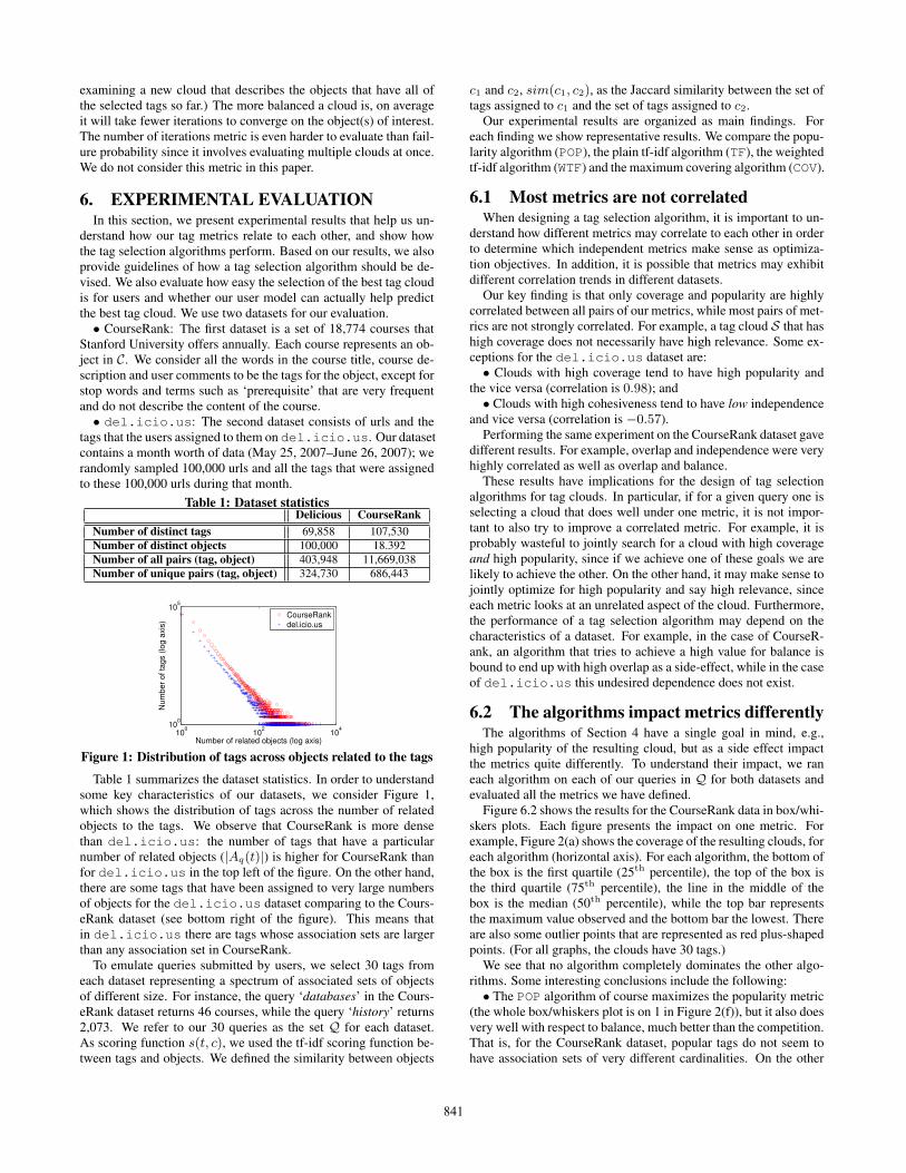
Figure 1: Distribution of tags across objects related to the tags

Table 1 summarizes the dataset statistics. In order to understandsome key characteristics of our datasets, we consider Figure 1,which shows the distribution of tags across the number of relatedobjects to the tags. We observe that CourseRank is more densethan del.icio.us: the number of tags that have a particularnumber of related objects (|Aq(t)|) is higher for CourseRank thanfor del.icio.us in the top left of the figure. On the other hand,there are some tags that have been assigned to very large numbersof objects for the del.icio.us dataset comparing to the Cours-eRank dataset (see bottom right of the figure). This means thatin del.icio.us there are tags whose association sets are largerthan any association set in CourseRank.

To emulate queries submitted by users, we select 30 tags fromeach dataset representing a spectrum of associated sets of objectsof different size. For instance, the query ‘databases’ in the Cours-eRank dataset returns 46 courses, while the query ‘history’ returns2,073. We refer to our 30 queries as the set Q for each dataset.As scoring function s(t, c), we used the tf-idf scoring function be-tween tags and objects. We defined the similarity between objects

c1 and c2, sim(c1, c2), as the Jaccard similarity between the set oftags assigned to c1 and the set of tags assigned to c2.

Our experimental results are organized as main findings. Foreach finding we show representative results. We compare the popu-larity algorithm (POP), the plain tf-idf algorithm (TF), the weightedtf-idf algorithm (WTF) and the maximum covering algorithm (COV).

6.1 Most metrics are not correlatedWhen designing a tag selection algorithm, it is important to un-

derstand how different metrics may correlate to each other in orderto determine which independent metrics make sense as optimiza-tion objectives. In addition, it is possible that metrics may exhibitdifferent correlation trends in different datasets.

Our key finding is that only coverage and popularity are highlycorrelated between all pairs of our metrics, while most pairs of met-rics are not strongly correlated. For example, a tag cloud S that hashigh coverage does not necessarily have high relevance. Some ex-ceptions for the del.icio.us dataset are:• Clouds with high coverage tend to have high popularity and

the vice versa (correlation is 0.98); and• Clouds with high cohesiveness tend to have low independence

and vice versa (correlation is −0.57).Performing the same experiment on the CourseRank dataset gave

different results. For example, overlap and independence were veryhighly correlated as well as overlap and balance.

These results have implications for the design of tag selectionalgorithms for tag clouds. In particular, if for a given query one isselecting a cloud that does well under one metric, it is not impor-tant to also try to improve a correlated metric. For example, it isprobably wasteful to jointly search for a cloud with high coverageand high popularity, since if we achieve one of these goals we arelikely to achieve the other. On the other hand, it may make sense tojointly optimize for high popularity and say high relevance, sinceeach metric looks at an unrelated aspect of the cloud. Furthermore,the performance of a tag selection algorithm may depend on thecharacteristics of a dataset. For example, in the case of CourseR-ank, an algorithm that tries to achieve a high value for balance isbound to end up with high overlap as a side-effect, while in the caseof del.icio.us this undesired dependence does not exist.

6.2 The algorithms impact metrics differentlyThe algorithms of Section 4 have a single goal in mind, e.g.,

high popularity of the resulting cloud, but as a side effect impactthe metrics quite differently. To understand their impact, we raneach algorithm on each of our queries in Q for both datasets andevaluated all the metrics we have defined.

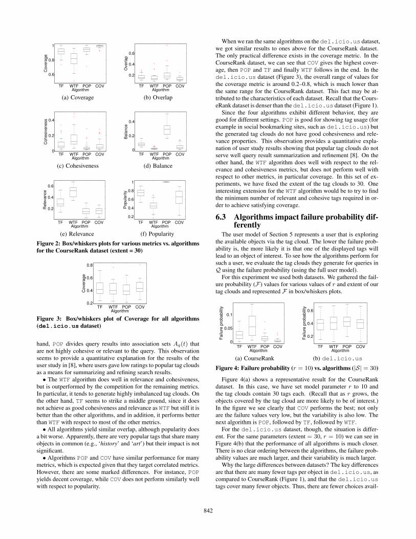
Figure 6.2 shows the results for the CourseRank data in box/whi-skers plots. Each figure presents the impact on one metric. Forexample, Figure 2(a) shows the coverage of the resulting clouds, foreach algorithm (horizontal axis). For each algorithm, the bottom ofthe box is the first quartile (25th percentile), the top of the box isthe third quartile (75th percentile), the line in the middle of thebox is the median (50th percentile), while the top bar representsthe maximum value observed and the bottom bar the lowest. Thereare also some outlier points that are represented as red plus-shapedpoints. (For all graphs, the clouds have 30 tags.)

We see that no algorithm completely dominates the other algo-rithms. Some interesting conclusions include the following:• The POP algorithm of course maximizes the popularity metric

(the whole box/whiskers plot is on 1 in Figure 2(f)), but it also doesvery well with respect to balance, much better than the competition.That is, for the CourseRank dataset, popular tags do not seem tohave association sets of very different cardinalities. On the other

841

TF WTF POP COV

0.6

0.8

1C

overa

ge

Algorithm

(a) Coverage

TF WTF POP COV

0.2

0.4

0.6

Overlap

Algorithm

(b) Overlap

TF WTF POP COV0

0.2

0.4

Cohesiv

eness

Algorithm

(c) Cohesiveness

TF WTF POP COV0

0.2

0.4B

ala

nce

Algorithm

(d) Balance

TF WTF POP COV

0.2

0.4

0.6

Rele

vance

Algorithm

(e) Relevance

TF WTF POP COV

0.2

0.4

0.6

0.8

1

Popula

rity

Algorithm

(f) Popularity

Figure 2: Box/whiskers plots for various metrics vs. algorithmsfor the CourseRank dataset (extent = 30)

TF WTF POP COV0.2

0.4

0.6

0.8

Co

ve

rag

e

Algorithm

Figure 3: Box/whiskers plot of Coverage for all algorithms(del.icio.us dataset)

hand, POP divides query results into association sets Aq(t) thatare not highly cohesive or relevant to the query. This observationseems to provide a quantitative explanation for the results of theuser study in [8], where users gave low ratings to popular tag cloudsas a means for summarizing and refining search results.• The WTF algorithm does well in relevance and cohesiveness,

but is outperformed by the competition for the remaining metrics.In particular, it tends to generate highly imbalanced tag clouds. Onthe other hand, TF seems to strike a middle ground, since it doesnot achieve as good cohesiveness and relevance as WTF but still it isbetter than the other algorithms, and in addition, it performs betterthan WTF with respect to most of the other metrics.• All algorithms yield similar overlap, although popularity does

a bit worse. Apparently, there are very popular tags that share manyobjects in common (e.g., ‘history’ and ‘art’) but their impact is notsignificant.• Algorithms POP and COV have similar performance for many

metrics, which is expected given that they target correlated metrics.However, there are some marked differences. For instance, POPyields decent coverage, while COV does not perform similarly wellwith respect to popularity.

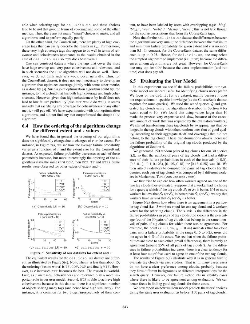
When we ran the same algorithms on the del.icio.us dataset,we got similar results to ones above for the CourseRank dataset.The only practical difference exists in the coverage metric. In theCourseRank dataset, we can see that COV gives the highest cover-age, then POP and TF and finally WTF follows in the end. In thedel.icio.us dataset (Figure 3), the overall range of values forthe coverage metric is around 0.2–0.8, which is much lower thanthe same range for the CourseRank dataset. This fact may be at-tributed to the characteristics of each dataset. Recall that the Cours-eRank dataset is denser than the del.icio.us dataset (Figure 1).

Since the four algorithms exhibit different behavior, they aregood for different settings. POP is good for showing tag usage (forexample in social bookmarking sites, such as del.icio.us) butthe generated tag clouds do not have good cohesiveness and rele-vance properties. This observation provides a quantitative expla-nation of user study results showing that popular tag clouds do notserve well query result summarization and refinement [8]. On theother hand, the WTF algorithm does well with respect to the rel-evance and cohesiveness metrics, but does not perform well withrespect to other metrics, in particular coverage. In this set of ex-periments, we have fixed the extent of the tag clouds to 30. Oneinteresting extension for the WTF algorithm would be to try to findthe minimum number of relevant and cohesive tags required in or-der to achieve satisfying coverage.

6.3 Algorithms impact failure probability dif-ferently

The user model of Section 5 represents a user that is exploringthe available objects via the tag cloud. The lower the failure prob-ability is, the more likely it is that one of the displayed tags willlead to an object of interest. To see how the algorithms perform forsuch a user, we evaluate the tag clouds they generate for queries inQ using the failure probability (using the full user model).

For this experiment we used both datasets. We gathered the fail-ure probability (F) values for various values of r and extent of ourtag clouds and represented F in box/whiskers plots.

TF WTF POP COV0

0.05

0.1

Fa

ilure

pro

ba

bili

ty

Algorithm

(a) CourseRank

TF WTF POP COV

0.2

0.4

0.6

Fa

ilure

pro

ba

bili

ty

Algorithm

(b) del.icio.us

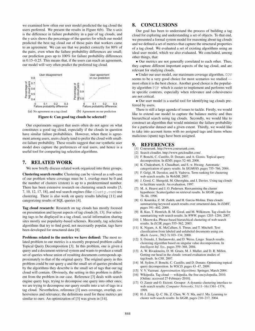
Figure 4: Failure probability (r = 10) vs. algorithms (|S| = 30)

Figure 4(a) shows a representative result for the CourseRankdataset. In this case, we have set model parameter r to 10 andthe tag clouds contain 30 tags each. (Recall that as r grows, theobjects covered by the tag cloud are more likely to be of interest.)In the figure we see clearly that COV performs the best; not onlyare the failure values very low, but the variability is also low. Thenext algorithm is POP, followed by TF, followed by WTF.

For the del.icio.us dataset, though, the situation is differ-ent. For the same parameters (extent = 30, r = 10) we can see inFigure 4(b) that the performance of all algorithms is much closer.There is no clear ordering between the algorithms, the failure prob-ability values are much larger, and their variability is much larger.

Why the large differences between datasets? The key differencesare that there are many fewer tags per object in del.icio.us, ascompared to CourseRank (Figure 1), and that the del.icio.ustags cover many fewer objects. Thus, there are fewer choices avail-

842

able when selecting tags for del.icio.us, and these choicestend to be not that good in terms of coverage and some of the othermetrics. Thus, there are not many “smart” choices to make, and allalgorithms tend to perform equally poorly.

On the other hand, for CourseRank, there are plenty of high cov-erage tags that can easily describe the results in Cq . Furthermore,these very high coverage tags also appear to do well in terms of rel-evance and cohesiveness (compared to the results obtained in thecase of del.icio.us), so COV does best overall.

One can construct datasets where the tags that cover the mosthave huge overlap and very poor cohesiveness and relevance, andin such scenarios the COV algorithm will not do as well. How-ever, we do not think such sets would occur naturally. Thus, forthe CourseRank dataset, it does not seem necessary to develop analgorithm that optimizes coverage jointly with some other metric,as is done by [3]. Such a joint optimization algorithm could try, forinstance, to find a cloud that has both high coverage and high cohe-siveness. However, given that high cohesiveness by itself does notlead to low failure probability (else WTF would do well), it seemsunlikely that sacrificing any coverage for cohesiveness (or any othermetric) will pay off. We have experimented with joint optimizationalgorithms, and did not find any that outperformed the simple COValgorithm.

6.4 How the ordering of the algorithms changefor different extent and r values

We have found that in general the ordering of our algorithmsdoes not significantly change due to changes of r or the extent. Forinstance, in Figure 5(a) we see how the average failure probabilityvaries as a function of r and the extent size for the CourseRankdataset. As expected, failure probability decreases as each of theseparameters increase, but more interestingly the ordering of the al-gorithms stays the same (first COV, then POP, TF and WTF). Sameresults were observed for other values of extent and r.

0 20 40 600

0.2

0.4

r

Failu

re p

robabili

ty

Failure probability vs.r (for extent = 10)

TFWTFPOPCOV

(a) CourseRank, |S| = 10

0 10 20 300

0.5

1

Extent

Failu

re p

robabili

ty

Failure probability vs.Extent (for r = 10)

TFWTFPOPCOV

(b) CourseRank, r = 10

0 20 40 600.4

0.6

0.8

r

Failu

re p

robabili

ty

Failure probability vs.r (for extent = 10)

TFWTFPOPCOV

(c) del.icio.us, |S| = 10

0 10 20 300

0.5

1

1.5

Extent

Failu

re p

robabili

ty

Failure probability vs.Extent (for r = 10)

TFWTFPOPCOV

(d) del.icio.us, r = 10

Figure 5: Sensitivity of our datasets for extent and r

The equivalent results for the del.icio.us dataset are differ-ent, as illustrated by Figure 5(c). Now, when r is less than about 15,the ordering (best to worst) is TF, COV, POP and finally WTF. How-ever, as r increases WTF becomes the best. The reason is twofold.First, as r increases, cohesiveness and relevance play a more im-portant role in our user model. Second, WTF is able to achieve highcohesiveness because in this data set there is a significant numberof objects sharing many tags (and hence have high similarity). Forinstance, it is common for two blogs, irrespectively of their con-

tent, to have been labeled by users with overlapping tags: ‘blog’,‘blogs’, ‘web’, ‘web2.0’, ‘design’, ‘news’; this is not true thoughfor the course descriptions that form the CourseRank tags.

Note that for the del.icio.us dataset the differences betweenthe algorithms are very small; the difference between the maximumand minimum failure probability for given extent and r is no morethan 0.1. In contrast, for the CourseRank dataset the same differ-ence is up to 0.25. Hence, for del.icio.us, one may selectthe simplest algorithm to implement (i.e., POP) because the differ-ences among algorithms are not great. However, for CourseRankone may opt for COV because the extra implementation (and runtime) cost does pay off.

6.5 Evaluating the User ModelIn this experiment we see if the failure probabilities our syn-

thetic model are indeed useful for identifying clouds users prefer.We focus on the del.icio.us dataset, mainly because it doesnot require domain-specific knowledge (as the CourseRank datasetrequires for some queries). We used the set of queries Q and gen-erated tag clouds using the algorithms described in Section 4 forextent equal to 10. (We found that using values larger than 10made the process very expensive and slow, because of the exces-sive amount of work that was required by the evaluators/workers.)We started transforming these tag clouds by swapping tags that be-longed in the tag clouds with other, random ones (but of good qual-ity, according to their aggregate tf-idf and coverage) that did notbelong to the tag cloud. These transformations always increasedthe failure probability of the original tag clouds produced by thealgorithms of Section 4.

We generated 150 random pairs of tag clouds for our 30 queries(Q), so that the number of pairs of tag clouds that had a differ-ence of their failure probabilities in each of the intervals [0, 0.5),[0.5, 0.1), [0.1, 0.125), [0.125, 0.15), or [0.15, 0.25) was 30. Wethen asked evaluators to compare the pairs of tag clouds for thequeries; each pair of tag clouds was compared by 5 different work-ers in Mechanical Turk (www.mturk.com).

We first tried to explore how often workers agreed on one of thetwo tag clouds they evaluated. Suppose that a worker had to choosefor a query q which of the tag clouds S1 or S2 is better. If 4 or moreworkers believe that S1 (or S2) is better than S2 (or S1), we say thatworkers have agreed that S1 (or S2) is better.

Figure 6(a) shows how often there is no agreement in a particu-lar tag cloud (i.e., 3 workers voted for one tag cloud and 2 workersvoted for the other tag cloud). The x-axis is the difference in thefailure probabilities in pairs of tag clouds; the y-axis is the percent-age (out of the 30 pairs of tag clouds that belong in the same inter-val) of pairs of tag clouds for which there was no agreement. Forexample, the point (x = 0.25, y = 0.44) indicates that for cloudpairs with a failure probability in the range 0.15 to 0.25, users didnot agree in 44% of the cases. We see that when the failure proba-bilities are close to each other (small differences), there is rarely anagreement (around 25% of all pairs of tag clouds!). As the differ-ence in failure probabilities increases, there is a clear tendency forat least four out of five users to agree on one of the two tag clouds.

The results of Figure 6(a) illustrate why it is in general hard toevaluate tag clouds via user studies. That is, in many cases usersdo not have a clear preference among clouds, probably becausethey have different backgrounds or different interpretations for thesearch query. However, our failure metric lets us identify caseswhere there is likely to be agreement among evaluators. We canhence focus in finding good tag clouds for those cases.

We now report on how well our model predicts the users’ choices.Using the same user evaluation as before (150 pairs of tag clouds),

843

we examined how often our user model predicted the tag cloud theusers preferred. We present the results in Figure 6(b). The x-axisis the difference in failure probability in a pair of tag clouds, andthe y-axis shows the percentage of the queries for which our modelpredicted the best tag cloud out of those pairs that workers cameto an agreement. We can see that we predict correctly for 80% ofthe pairs, even when the failure probability differences are small;our prediction goes up to 100% for failure probability differencesin 0.15–0.25. This means that, if the users can reach an agreement,our model will very often predict the preferred tag cloud.

0 0.1 0.2 0.3

0.4

0.5

0.6

0.7

0.8

Failure probability difference

Perc

enta

ge o

fta

g c

loud p

airs

User disagreement

(a) No agreement on a tag cloud

0 0.1 0.2 0.3

0.8

0.9

1

Failure probability difference

Perc

enta

ge o

fta

g c

loud p

airs

User agreementon our prediction

(b) Agreement on our prediction

Figure 6: Can good tag clouds be selected?

Our experiments suggest that users often do not agree on whatconstitutes a good tag cloud, especially if the clouds in questionhave similar failure probabilities. However, when there is agree-ment among users, users clearly tend to prefer the cloud with small-est failure probability. These results suggest that our synthetic usermodel does capture the preferences of real users, and hence is auseful tool for comparing tag selection algorithms.

7. RELATED WORKWe now briefly discuss related work organized into three groups.

Clustering search results: Clustering can be viewed as a sub-caseof our problem where coverage must be 1, overlap must be 0 andthe number of clusters (extent) is up to a predetermined number.There has been extensive research on clustering search results [5,7, 10, 12, 17, 18], and real search engines (like clusty.com) useclustering. There is also work on query results labeling [11] andcategorizing results of SQL queries [4].

Tag cloud research: Research on tag clouds has mostly focusedon presentation and layout aspects of tag clouds [6, 13]. For select-ing tags to be displayed in a tag cloud, social information sharingsites mostly use popularity-based schemes. Recently, tag selectionalgorithms that try to find good, not necessarily popular, tags havebeen developed for structured data [8].

Problems related to the metrics we have defined: The most re-lated problem to our metrics is a recently proposed problem calledTopical Query Decomposition [3]. In this problem, one is given aquery and a document retrieval system and wants to produce a smallset of queries whose union of resulting documents corresponds ap-proximately to that of the original query. The original query in thisproblem could be our query q and the small set of queries producedby the algorithms they describe is the small set of tags that our tagcloud will contain. Obviously, the setting in this problem is differ-ent from the problem in our case. Reference [3] deals with searchengine query logs, trying to decompose one query into other ones;we are trying to decompose our query results into a set of tags in atag cloud. Nevertheless, reference [3] uses coverage, overlap, co-hesiveness and relevance; the definitions used for these metrics aresimilar to ours. An optimization of [3] was given in [14].

8. CONCLUSIONSOur goal has been to understand the process of building a tag

cloud for exploring and understanding a set of objects. To that end,we presented a formal system model for reasoning about tag cloudsand we defined a set of metrics that capture the structural propertiesof a tag cloud. We evaluated a set of existing algorithms using anideal user model, which we also evaluated. We concluded, amongother things, that:• Our metrics are not generally correlated to each other. Thus,

they capture different important aspects of the tag cloud, and arerelevant for studying clouds.• Under our user model, our maximum coverage algorithm, COV

seems to be a very good choice for most scenarios we studied —most often it is the best choice. Another good choice is the popular-ity algorithm POP which is easier to implement and performs wellin specific contexts, especially when relevance and cohesivenessare not critical.• Our user model is a useful tool for identifying tag clouds pre-

ferred by users.There is still a large agenda of issues to tackle. Firstly, we would

like to extend our model to capture the balance metric and thushierarchical search using tag clouds. Secondly, we would like toconstruct an algorithm that would minimize the failure probabilityfor a particular dataset and a given extent. Thirdly, we would liketo take into account items with no assigned tags and items wheremalicious (spam) tags have been assigned.

9. REFERENCES[1] Courserank. http://www.courserank.com.[2] Search cloudlet. http://www.getcloudlet.com/.[3] F. Bonchi, C. Castillo, D. Donato, and A. Gionis. Topical query

decomposition. In KDD, pages 52–60, 2008.[4] K. Chakrabarti, S. Chaudhuri, and S.-w. Hwang. Automatic

categorization of query results. In SIGMOD, pages 755–766, 2004.[5] F. Gelgi, H. Davulcu, and S. Vadrevu. Term ranking for clustering

web search results. In WebDB, 2007.[6] J. Good, C. Shergold, M. Gheorghiu, and J. Davies. Using tag clouds

to facilitate search: An evaluation, 1997.[7] M. A. Hearst and J. O. Pedersen. Reexamining the cluster

hypothesis: Scatter/gather on retrieval results. In SIGIR, pages76–84, 1996.

[8] G. Koutrika, Z. M. Zadeh, and H. Garcia-Molina. Data clouds:summarizing keyword search results over structured data. In EDBT,pages 391–402, 2009.

[9] B. Kuo, T. Hentrich, B. M. Good, and M. Wilkinson. Tag clouds forsummarizing web search results. In WWW, pages 1203–1204, 2007.

[10] I. Masowska. Phrase-based hierarchical clustering of web searchresults. In ECIR, pages 555–562, 2003.

[11] K. Nigam, A. K. McCallum, S. Thrun, and T. Mitchell. Textclassification from labeled and unlabeled documents using em.Mach. Learn., 39(2-3):103–134, 2000.

[12] S. Osinski, J. Stefanowski, and D. Weiss. Lingo: Search resultsclustering algorithm based on singular value decomposition. InIntelligent Inf. Sys., pages 359–368, 2004.

[13] A. W. Rivadeneira, D. M. Gruen, M. J. Muller, and D. R. Millen.Getting our head in the clouds: toward evaluation studies oftagclouds. In CHI, 2007.

[14] M. Sydow, F. Bonchi, C. Castillo, and D. Donato. Optimising topicalquery decomposition. In WSCD, pages 43–47, 2009.

[15] V. V. Vazirani. Approximation Algorithms. Springer, March 2004.[16] Wikipedia. Tag cloud — wikipedia, the free encyclopedia, 2010.

[Online; accessed 27-February-2010].[17] O. Zamir and O. Etzioni. Grouper: A dynamic clustering interface to

web search results. Computer Networks, 31(11–16):1361–1374,1999.

[18] H.-J. Zeng, Q.-C. He, Z. Chen, W.-Y. Ma, and J. Ma. Learning tocluster web search results. In SIGIR, pages 210–217, 2004.

844