Chapter 8: Tropical Tropopause Layer - SPARC
82
307 -- Early online release -- Chapter 8: Tropical Tropopause Layer Abstract. This chapter evaluates the tropical transition region between the well-mixed, convective troposphere and the highly stratified stratosphere in the reanalyses. The general tropical tropopause layer structure, as given by the vertical temperature profile, tropopause levels, and the level of zero radiative heating, is analysed. Diagnostics related to clouds and convection in the tropical tropopause layer include cloud fraction, cloud water content, and outgoing longwave radiation. The chapter takes into account the diabatic heat budget as well as dynamical charac- teristics of the tropical tropopause layer such as Lagrangian cold points, residence times, and wave activity. Finally, the width of the tropical belt based on tropical and extra-tropical diagnostics and the representation of the South Asian Summer Monsoon in the reanalyses are evaluated. Thomas Birner (1) Meteorological Institute, Ludwig-Maximilians-University Munich (2) Institute of Atmospheric Physics, German Aerospace Center (DLR Oberpfaffenhofen) previously at: Department of Atmospheric Science, Colorado State University, USA Germany Nicholas A. Davis Atmospheric Chemistry Observations & Modeling Lab, National Center for Atmos- pheric Research, Boulder, CO USA Sean Davis Chemical Sciences Laboratory, National Oceanic and Atmospheric Administration USA Masatomo Fujiwara Faculty of Environmental Earth Science, Hokkaido University Japan Cameron R. Homeyer School of Meteorology, University of Oklahoma, USA Ioana Ivanciu GEOMAR Helmholtz-Zentrum für Ozeanforschung Kiel Germany Young-Ha Kim Goethe University Frankfurt Germany Bernard Legras Laboratoire de Météorologie Dynamique, CNRS/ENS-PSL France Gloria L. Manney (1) NorthWest Research Associates (2) New Mexico Institute of Mining and Technology USA Eriko Nishimoto NTT DATA INTELLILINK Corporation previously at: Japan Agency for Marine Earth Science and Technology Japan Matthias Nützel Institute of Atmospheric Physics, German Aerospace Center (DLR Oberpfaffenhofen) Germany Robin Pilch Kedzierski GEOMAR Helmholtz-Zentrum für Ozeanforschung Kiel Germany James S. Wang Institute for Advanced Sustainability Studies Germany Tao Wang Jet Propulsion Laboratory, California Institute of Technology USA Jonathon S. Wright Department of Earth System Science, Tsinghua University China Susann Tegtmeier Institute of Space and Atmospheric Studies, University of Saskatchewan previously at: GEOMAR Helmholtz Centre for Ocean Research Kiel, Germany Canada Kirstin Krüger Section for Meteorology and Oceanography, Department of Geosciences, University of Oslo Norway Chapter lead authors Co-authors
-
Upload
khangminh22 -
Category
Documents
-
view
1 -
download
0
Transcript of Chapter 8: Tropical Tropopause Layer - SPARC

307
-- Early online release --
Chapter 8: Tropical Tropopause Layer
Abstract. This chapter evaluates the tropical transition region between the well-mixed, convective troposphere and the highly stratified stratosphere in the reanalyses. The general tropical tropopause layer structure, as given by the vertical temperature profile, tropopause levels, and the level of zero radiative heating, is analysed. Diagnostics related to clouds and convection in the tropical tropopause layer include cloud fraction, cloud water content, and outgoing longwave radiation. The chapter takes into account the diabatic heat budget as well as dynamical charac-teristics of the tropical tropopause layer such as Lagrangian cold points, residence times, and wave activity. Finally, the width of the tropical belt based on tropical and extra-tropical diagnostics and the representation of the South Asian Summer Monsoon in the reanalyses are evaluated.
Thomas Birner(1) Meteorological Institute, Ludwig-Maximilians-University Munich(2) Institute of Atmospheric Physics, German Aerospace Center (DLR Oberpfaffenhofen)previously at: Department of Atmospheric Science, Colorado State University, USA
Germany
Nicholas A. Davis Atmospheric Chemistry Observations & Modeling Lab, National Center for Atmos-pheric Research, Boulder, CO USA
Sean Davis Chemical Sciences Laboratory, National Oceanic and Atmospheric Administration USA
Masatomo Fujiwara Faculty of Environmental Earth Science, Hokkaido University Japan
Cameron R. Homeyer School of Meteorology, University of Oklahoma, USA
Ioana Ivanciu GEOMAR Helmholtz-Zentrum für Ozeanforschung Kiel Germany
Young-Ha Kim Goethe University Frankfurt Germany
Bernard Legras Laboratoire de Météorologie Dynamique, CNRS/ENS-PSL France
Gloria L. Manney (1) NorthWest Research Associates (2) New Mexico Institute of Mining and Technology USA
Eriko Nishimoto NTT DATA INTELLILINK Corporationpreviously at: Japan Agency for Marine Earth Science and Technology Japan
Matthias Nützel Institute of Atmospheric Physics, German Aerospace Center (DLR Oberpfaffenhofen) Germany
Robin Pilch Kedzierski GEOMAR Helmholtz-Zentrum für Ozeanforschung Kiel Germany
James S. Wang Institute for Advanced Sustainability Studies Germany
Tao Wang Jet Propulsion Laboratory, California Institute of Technology USA
Jonathon S. Wright Department of Earth System Science, Tsinghua University China
Susann Tegtmeier Institute of Space and Atmospheric Studies, University of Saskatchewanpreviously at: GEOMAR Helmholtz Centre for Ocean Research Kiel, Germany Canada
Kirstin Krüger Section for Meteorology and Oceanography, Department of Geosciences, University of Oslo Norway
Chapter lead authors
Co-authors

308
-- Early online release --
SPARC Reanalysis Intercomparison Project (S-RIP) Final Report -- Early online release --
Contents8.1 Introduction ................................................................................................................................................3098.2 Temperature and tropopause characteristics .......................................................................................... 310
8.2.1 Observational data sets ......................................................................................................................3108.2.2 Climatology .........................................................................................................................................3108.2.3 Interannual variability and long-term changes ...............................................................................3138.2.4 Key findings and recommendations .................................................................................................315
8.3 Clouds and convection .............................................................................................................................. 3168.3.1 Observational data sets ......................................................................................................................3168.3.2 Spatial distribution of high clouds ....................................................................................................3188.3.3 Vertical profiles ..................................................................................................................................3198.3.4 Cloud radiative effects .......................................................................................................................3218.3.5 Relationships with other variables ...................................................................................................3248.3.6 Temporal variability ...........................................................................................................................3268.3.7 Key findings and recommendations .................................................................................................328
8.4 Diabatic heating rates ................................................................................................................................3298.4.1 Total diabatic heating ........................................................................................................................3298.4.2 Radiative heating .................................................................................................................................3308.4.3 Non-radiative heating ........................................................................................................................3358.4.4 Key findings and recommendations .................................................................................................336
8.5 Transport ....................................................................................................................................................3378.5.1 Dehydration point distribution .........................................................................................................3378.5.2 TTL residence time .............................................................................................................................3398.5.3 TTL tropical upwelling .......................................................................................................................3418.5.4 Key findings and recommendations .................................................................................................341
8.6 Wave activity ..............................................................................................................................................3438.6.1 Horseshoe-shaped structure at the 100 hPa temperature ...............................................................3438.6.2 Equatorial waves .................................................................................................................................3448.6.3 Key findings .........................................................................................................................................346
8.7 Width of the TTL....................................................................................................................................... 3468.7.1 Zonally-resolved subtropical jet diagnostic ....................................................................................3478.7.2 Zonally-resolved tropopause break diagnostic ................................................................................3498.7.3 Zonal mean subtropical jet and tropopause break diagnostics .....................................................3508.7.4 Key findings and recommendations .................................................................................................351
8.8 South Asian Summer Monsoon ...............................................................................................................3518.8.1 Anticyclone: climatology and variability .........................................................................................3528.8.2 Vertical velocity ...................................................................................................................................3578.8.3 Diabatic heating ..................................................................................................................................3598.8.4 Transport..............................................................................................................................................3618.8.5 Ozone ...................................................................................................................................................3628.8.6 Regional analysis of clouds and radiative effects .............................................................................3648.8.7 Key findings and recommendations .................................................................................................369
8.9 Summary, Key Findings, and Recommendations ..................................................................................370References .............................................................................................................................................................374Appendix A: Supplementary material ..............................................................................................................380Major abbreviations and terms ..........................................................................................................................386

309Chapter 8: Tropical Tropopause Layer
-- Early online release --
-- Early online release --
8.1 Introduction
The tropical tropopause layer (TTL) is the transition region between the well mixed, convective troposphere and the radi-atively controlled stratosphere. The vertical range of the TTL extends from the region of strong convective outflow near 12 - 14 km to highest altitudes influenced by convective over-shooting and tropical tropospheric processes up to 18.5 km (Fig. 8.1; Folkins et al., 1999; Highwood and Hoskins, 1998). Air masses in the TTL show dynamical and chemical prop-erties of both the troposphere and the stratosphere and are controlled by numerous processes on a wide range of length- and time scales (e.g., Fueglistaler et al., 2009a). The complex interactions of circulation, convection, trace gases, clouds and radiation make the TTL a key player in radiative forcing and chemistry-climate coupling (e.g., Randel and Jensen, 2013). Most important, the TTL is the main gateway for air entering the stratosphere. Therefore, stratospheric composition and chemistry, in particular of ozone, water vapour and aerosols, is strongly impacted by the composition of air near the trop-ical tropopause (e.g., Fueglistaler et al., 2011; Holton and Get-telman, 2001). The cold point in the inner tropics is of special importance for air masses on their way from the troposphere into the stratosphere, since it sets their stratospheric water va-por content (e.g., Randel et al., 2004; Mote et al., 1996). Togeth-er with clouds, such as thin cirrus and convective anvils, wa-ter vapor in the TTL has a significant impact on the radiation and tropospheric climate. In general, the chemical and ther-mal boundary conditions of the TTL are determined by the interplay of rapid tropospheric convection, the stratospheric wave-driven circulation and exchange with mid-latitude air.
Reanalyses provide vertical and horizontal structures for temperature, geopotential height, wind, radiation budgets and cloud properties that are important for studies of atmos-pheric transport, dynamics and composition in the TTL. Many off-line chemistry-transport models and Lagrangi-an particle dispersion models are driven by reanalysis data (e.g., Schoeberl et al., 2012; Krüger et al., 2009; Chipperfield, 1999). Their representation of the cold point determines how
realistically such models simulate dehydration and the en-trainment of trace gases or aerosols into the stratosphere. Process studies of TTL dynamics such as equatorial wave variability are also often based on the TTL temperature structure in reanalyses (e.g., Fujiwara et al., 2012). Finally, reanalysis cold point temperature and height have been used in the past for comparison to model results and for inves-tigations of long-term changes (e.g., Gettelman et al., 2010). While many studies have highlighted the characteristics of individual reanalysis products, a comprehensive intercom-parison of the TTL among all major atmospheric reanalyses is currently missing.
Given the steep vertical gradient of atmospheric properties in the TTL, the vertical resolution of the reanalysis data is important. Reanalysis models resolve the TTL with different vertical resolutions, as illustrated in Figure 8.2. The number of model levels between 200 hPa and 70 hPa varies among the reanalyses from a low of 4 (NCEP-NCAR R1) to a high of 21 (ERA5), corresponding to vertical resolutions between ~1.5 km and ~0.2 km. In addition to the native model levels, all reanalyses provide post-processed data on fixed standard
pressure levels with four levels situated between 200 and 70 hPa (Fig. 8.2). Detailed descriptions of the reanalysis data and their assimilated observa-tions can be found in Chapter 2 and Fujiwara et al. (2017). If not mentioned otherwise, the MERRA and MERRA-2 ASM products are used.
This chapter investigates whether reanalysis data reproduce the key characteristics of the TTL, including basic processes, such as circulation patterns, radiation and large-scale wave forc-ing, and their variability in space and time. The general TTL structure as given by the cold point and lapse rate tropopause and the vertical tem-perature profile is evaluated in Section 8.2. Diag-nostics on clouds and convection in the TTL in-clude cloud fraction profiles, outgoing longwave radiation, and cloud water content (Section 8.3). Figure 8.1: Schematic of the Tropical Tropopause Layer (TTL).
ERA-Interim ERA5 JRA-25 JRA-55 MERRA MERRA-2 R1 CFSR PL
80
100
120
140
160
180
Pres
sure
(hPa
)
Model levels for the TTL region
Figure 8.2: Model-level pressure values for different re-analysis data sets in the TTL using a fixed surface pressure of 1013.25 hPa. Standard pressure levels (PL) in the TTL region are also shown. Adapted from Tegtmeier et al. (2020).

310
-- Early online release --
SPARC Reanalysis Intercomparison Project (S-RIP) Final Report -- Early online release --
suffer from inhomogeneities or time-varying biases due to changes in instruments or measurement practices (Sei-del and Randel, 2006). Adjusted radiosonde temperature at 100 hPa, 70 hPa and corresponding trends at the cold point have been created by removing such inhomogeneities (Wang et al., 2012, and references therein). In Section 8.2, we use several independently adjusted radiosonde data sets, including RATPAC (Free et al., 2005), RAOBCORE (Haim-berger, 2007) and HadAT (Thorne et al., 2005) as well as the unadjusted, quality-controlled radiosonde data set IGRA (Durre et al., 2006) covering the S-RIP core time period (1980 - 2010) (see Chapter 1, Section 1.2).
Since 2002, high-resolution temperature and pressure data in the TTL are also available from satellite retrievals based on the Global Navigation Satellite System – Radio Occultation (GNSS-RO) technique. Recent studies have demonstrated good agreement between GNSS-RO and ra-diosonde temperature profiles (e.g., Ho et al., 2017; Anthes et al., 2008). In Sections 8.2 and 8.8, we use zonal mean as well as gridded (5 ° × 5 °) tropopause data sets constructed from GNSS-RO measurements collected by the Challeng-ing Minisat Payload (CHAMP, Wickert et al., 2001), Grav-ity Recovery and Climate Experiment (GRACE, Beyerle et al., 2005), Constellation Observing System for Meteor-ology, Ionosphere, and Climate (COSMIC, Anthes et al., 2008), Metop-A (von Engeln et al., 2011), Metop-B, Satélite de Aplicaciones Científicas-C/Scientific Application Satel-lite-C (SAC-C, Hajj et al., 2004), and TerraSAR-X (Beyerle et al., 2011) missions. All data are re-processed or post-pro-cessed occultation profiles with moisture information (‘wetPrf ’ product) as provided by the COSMIC Data Anal-ysis and Archive Center (CDAAC, https://cdaac-www.cosmic.ucar.edu/cdaac/products.html). Observational temperature records at reanalysis model levels in the TTL region have been determined by interpolating GNSS-RO temperature profiles with the barometric formula, taking into account the lapse rate between levels. For each profile, the cold point and lapse rate tropopause characteristics were identified based on the cold point and WMO criteria (World Meteorological Organization, 1957), respectively.
8.2.2 Climatology
Given the strong gradients of temperature and static sta-bility in the TTL, the vertical resolution of the reanalysis data is an important factor in determining the cold point and lapse rate tropopause. For each reanalysis, tropopause heights and temperatures can be derived either from mod-el- or pressure-level data. A comparison of the CFSR cold point tropopause based on model- and pressure-level tem-perature data is shown here to demonstrate the clear ad-vantage of the finer model-level resolution (Fig. 8.3). The cold point tropopause from CFSR model-level data for the time period 2002 - 2010 agrees well with radio occultation results, with differences of less than 1.5 K and 0.2 km at all latitudes. The tropopause derived from CFSR pressure-lev-el data, on the other hand, shows larger differences.
This chapter also takes into account the diabatic heating rates (Section 8.4) as well as dynamical characteristics of the TTL such as transport processes (Section 8.5), wave ac-tivity (Section 8.6), and long-term changes of the width of the TTL (Section 8.7). Analysis of the South Asian Summer Monsoon highlights spatial and temporal variations with-in the TTL (Section 8.8). Finally, Chapter 8 is summarized in Section 8.9.
8.2 Temperature and tropopause characteristics
The tropopause is the most important physical bounda-ry within the TTL, serving to separate the turbulent, moist troposphere from the stable, dry stratosphere. The position of the tropopause is diagnosed by the thermal properties of the TTL, as a negative, tropospheric vertical temperature gradi-ent changes into a positive stratospheric temperature gradient. The role of the tropopause as a physical boundary is evident not only from the vertical temperature structure, but also from the distributions of atmospheric trace gases and clouds.
In the tropics, two definitions of the tropopause are wide-ly used: one based on the cold point and one based on the characteristics of the lapse rate. The cold point tropopause is defined as the level at which the vertical temperature profile reaches its minimum (Highwood and Hoskins, 1998) and air parcels en route from the troposphere to the stratosphere encounter the lowest temperatures. Final dehydration typ-ically occurs at these lowest temperatures, so that the cold point tropopause effectively controls the overall water va-pour content of the lower stratosphere (Randel et al., 2004) and explains its variability (Fueglistaler et al., 2009a). While the cold point tropopause is an important boundary in the tropics where upwelling predominates, this definition of the tropopause is irrelevant for water vapor transport into the stratosphere at higher latitudes where net downwelling oc-curs. The lapse rate tropopause, on the other hand, offers a globally-applicable definition of the tropopause, defined as the lowest level at which the lapse rate decreases to 2 K km-1 or less, provided that the average lapse rate between this lev-el and all higher levels within 2 km does not exceed 2 K km-1 (World Meteorological Organization, 1957). The tropical lapse rate tropopause is typically ~0.5 km (~10 hPa) lower and ~1 K warmer than the cold point tropopause (Seidel et al., 2001). In Section 8.2, we present a climatology of the tropical tropopause as derived from modern reanalysis data sets and compare it to data from high resolution measure-ments such as radiosondes or radio occultation. We also investigate temporal variability and long-term changes of TTL and cold point temperatures. All evaluations and fur-ther investigations can be found in Tegtmeier et al. (2020).
8.2.1 Observational data sets
High-resolution observations of the TTL are available from radiosonde stations in the tropics. However, climate records of radiosonde temperature, height and pressure data often

311Chapter 8: Tropical Tropopause Layer
-- Early online release --
-- Early online release --
This estimate is up to 0.4 km too low and up to 3 K too warm, illustrating the need to use data with high vertical resolution to identify and describe the tropopause. The fol-lowing climatological tropopause comparisons are all based on model-level data.
Tropical mean temperatures from reanalyses at two stand-ard pressure levels (100 hPa and 70 hPa) and at the two trop-opause levels are compared to radio occultation data for the time period 2002 - 2010 (Fig. 8.4). At 100 hPa, reanalysis temperatures agree well with radio occultation observa-tions with differences between - 0.35 K (too cold; ERA-In-terim and ERA5) and 0.43 K (too warm; CFSR). At 70 hPa, the agreement is even better, with differences ranging from - 0.29 K (JRA-55) to 0.12 K (JRA-25). However, nearly all re-analyses show warm biases at both tropopause levels, with differences of up to 1.2 K compared to the observations. Most likely, the excess warmth of tropopause estimates based on reanalysis products stems from the limited vertical resolution of the reanalysis models in the TTL region. The best agreement is found for the reanalysis with the highest vertical resolution here (ERA5; 0.05 K too warm at the cold point tropopause). The reanalysis with the lowest vertical resolution (NCEP-NCAR R1) is 2.2 K too warm, outside the range displayed in Figure 8.4.
Temperature profile comparisons between 140 hPa and 70 hPa at the native model level resolution have been con-ducted for the five most recent reanalyses (ERA5, ERA-In-terim, JRA-55, MERRA-2, CFSR). All reanalyses tend to be colder than the observations in the tropical mean (Fig. 8.5), but differences are relatively small, and the agreement is good overall. CFSR and ERA5 agree best with the radio occultation data with mean biases of around - 0.06 K and - 0.28 K, respectively, averaged over the whole vertical range. ERA-Interim and MERRA-2 agree very well at upper levels but show relatively large deviations near 100 hPa (ERA-Inter-im; - 0.82 K) and below 110 hPa (MERRA-2; - 0.67 K), respec-tively. The evaluation demonstrates that temperature com-parisons at standard pressure levels (Fig. 8.4) can be biased by up to 0.5 K, with CFSR showing a positive bias (0.45 K)
at the 100 hPa standard pressure level but very good agreement (- 0.05 K) at nearby native mod-el levels. Such biases can result from vertical interpolation of temperature data in regions with large lapse rate changes.
Comparing the temperature profiles to the tropopause val-ues (Figs. 8.4 and 8.5) reveals that despite the five reanalyses having negative biases at mod-el levels, they mostly have posi-tive biases at the cold point and lapse rate tropopause levels.
-20 0 20
latitude [ ]o
90
95
100
Pressure [hPa]
-20 0 2016.6
16.8
17
17.2
Altitude [km]
CFSR model levels CFSR pressure levels GNSS-RO
-20 0 20190
195
200
205Temperature [K]
Cold Point Tropopause 2002 - 2010
latitude [ ]o latitude [ ]o
Figure 8.3: Latitudinal distributions of annual mean, zonal mean cold point tropopause pressure (left), altitude (centre) and temperature (right) based on radio occulta-tion data (black) and CFSR model-level (green solid) and pressure-level (green dashed) data during 2002–2010. Adapted from Tegtmeier et al. (2020).
192 193 194 195 196 197 198 199temperature [K]
100 hPa
LRT
CPT
70 hPa
Temperature (20S-20N), 2002-2010
ERA-InterimERA5JRA-25JRA-55MERRAMERRA-2CFSRGNSS-RO -0.5 0 0.5 1
temperature [K]
100 hPa
LRT
CPT
70 hPa
Reanalysis - GNSS-RO, 2002-2010
Figure 8.4: Tropical mean (20 ° S - 20 ° N), annual mean temperatures at 100 hPa, the lapse rate tropopause (LRT), the cold point tropopause (CPT) and 70 hPa from reanalyses and GNSS-RO observations during 2002 - 2010 (left panel). Differences between the re-analysis and GNSS-RO temperatures are shown in the right panel. At 100 hPa, ERA-Interim is hidden by ERA-5; at the LRT, MERRA-2 is hidden by JRA-55; and at 70 hPa, ERA5 is hidden by JRA-25 and MERRA is hidden by MERRA-2. Adapted from Tegtmeier et al. (2020).
194 196 198 200temperature [K]
70
80
90
100
110
120
130
140
pres
sure
[hPa
]
Temperature (20S-20N), 2002-2010
ERA5ERA-InterimJRA-55MERRA-2CFSRGNSS-RO
-1 -0.5 0temperature [K]
70
80
90
100
110
120
130
140
Reanalysis - GNSS-RO
Figure 8.5: Tropical mean (20°S–20°N), annual mean tem-perature profiles at reanalysis model levels between 140 and 70 hPa (left panel) during 2002–2010 and differences be-tween reanalyses and GNSS-RO temperatures (right panel). Adapted from Tegtmeier et al. (2020).

312
-- Early online release --
SPARC Reanalysis Intercomparison Project (S-RIP) Final Report -- Early online release --
As the discrete values corresponding to reanalysis model levels are unable to reproduce the observed min-imum temperature as recorded in a near-continuous profile, this difference is expected for the cold point tropopause. Similarly, the lapse rate tropopause criteria might typically be fulfilled at lower levels for data at coarser resolution, thus resulting in a warm bias at the lapse rate tropopause on average. Overall, our results indicate that the negative temperature bias at model levels is more than cancelled out by the positive bias introduced when calculating the cold point and lapse rate tropopauses. Linking the temperature profile and tropopause comparisons, this ‘bias shift’ is about 0.3 K for ERA5, 0.6 K for CFSR and 1 K or larger for ERA-In-terim, MERRA-2 and JRA-55. In consequence, ERA5, with both a small negative bias at the model levels and a small bias shift provides the most realistic tropopause temperatures compared to GNSS-RO observations. CFSR also has a relatively small bias shift, but the most-ly unbiased temperature profile does not permit any error cancelation via this shift, so that cold point and lapse rate tropopause levels based on CFSR are system-atically too warm.
Agreement of the reanalysis temperature profiles from ERA5, ERA-Interim, MERRA-2, and CFSR with GNSS-RO data clearly improves for the comparison restricted to the 2007–2010 time period, when the more dense-ly-sampled COSMIC data were assimilated (Fig. A8.1 in Appendix A). Cold biases at model levels are accom-panied by warm biases in the tropopause temperatures, which, for ERA-Interim and ERA5, increase after 2007. Here, the advantage of a reduced temperature bias at model levels comes at the expense of an increased tem-perature bias at the tropopause.
Evaluations of the latitudinal structure of the cold point tropopause for 2002 - 2010 are based on compari-sons to radio occultation data (Fig. 8.6). All reanalysis data produce tropopause levels that are too low and too warm, with the latter related to vertical resolution as ex-plained above. The observations show that average cold point temperatures are lowest right around the equator. The reanalyses fail to reproduce this latitudinal gradi-ent, indicating more constant cold point temperatures across the inner tropics between 10 ° S and 10 ° N with a less pronounced minimum at the equator. As a conse-quence, the largest differences in cold point tropopause temperatures relative to GNSS-RO data are at the equa-tor and the best agreement is around 20 ° S/20 ° N for all reanalysis data.
The cold point altitude and pressure exhibit little north–south variability, ranging from 16.9 km (94 hPa) to 17.2 km (91.8 hPa). The lowest cold point tempera-tures are located near the equator, while the highest cold point altitudes are located around 20 ° S/20 ° N due to zonally-variable tropospheric pressure regimes, such as particularly low tropopause pressures over the Tibetan plateau during boreal summer (Kim and Son, 2012). The reanalysis data capture most of this latitu-dinal structure, showing roughly constant differences between about 0.1 km and 0.2 km (0 - 2 hPa, Fig. 8.6). The largest differences are found for NCEP-NCAR R1 in the SH, where the cold point tropopause based on R1 is both higher and warmer than observed. The best agree-ment with respect to cold point temperatures is found for ERA5 and ERA-Interim, which are around 0.2 K and 0.4 K warmer than the radio occultation data, respec-tively. All other reanalysis data are in close agreement with each other, with differences from the observations
of between 0.5 K and 1 K. The alti-tude and pressure of the cold point tropopause are captured best by ERA5, CFSR, MERRA, MERRA-2 and JRA-55, which all produce cold point tropopauses that are slightly too low (~0.1 km). ERA-Interim, despite very good agreement in cold point temperature, shows slightly larger biases in cold point altitude (~0.2 km) relative to the GNSS-RO benchmark.
Differences between reanalyses (ERA-Interim, MERRA-2, JRA55, and CFSR) and observations are largest in the inner tropics over cen-tral Africa, reaching values 50 % to 100 % greater than the zonal mean differences (Fig. A8.2 in Appen-dix A). This region is characterized by a local cold point minimum that results from deep convection and its interaction with equatorial waves.
ERA5
Cold Point Tropopause, 2002 - 2010
Reanalyses - GNSS-RO, 2002 - 2010
mERA-Interi JRA-25
JRA-55 CFSR
R1MERRA
MERRA-2GNSS-RO
-20 0 20190
192
194
196
198
tem
pera
ture
[K]
-20 0 2016.8
17
17.2
17.4
altit
ude
[km
]
-20 0 20
88
90
92
94
96
pres
sure
[hPa
]temperature altitude pressure
-20 0 20latitude [°]
0
1
2
tem
pera
ture
[K]
-20 0 20latitude [°]
-0.3
-0.2
-0.1
0
altit
ude
[km
]
-20 0 20latitude [°]
-2
0
2
4pres
sure
[hPa
]
Figure 8.6: Latitudinal distributions of zonal-mean cold point tropopause tem-perature (left), altitude (centre) and pressure (right) based on radio occultation data and reanalysis products during 2002 - 2010 (upper row) derived from model level data. Differences between reanalysis and radio occultation estimates are shown in the lower row. Adapted from Tegtmeier et al. (2020).

313Chapter 8: Tropical Tropopause Layer
-- Early online release --
-- Early online release --
8.2.3 Interannual variability and long-term changes
The interannual variability of TTL temperatures is strongly affected by both tropospheric (e.g., ENSO) and stratospheric (e.g., QBO, solar, vol-canic) variability (Krüger et al., 2008; Zhou et al., 2001; Randel et al., 2000). Time series of 70 hPa temperature anomalies and cold point tempera-ture, pressure and altitude anoma-lies deseasonalized with respect to the common time period 2002 - 2010 are shown in Figure 8.8. The perfor-mance of the reanalyses with respect to both the spread among reanalyses and their agreement with observa-tions is much better at the 70 hPa level than at the cold point level. Here, mostly the older reanalyses NCEP-NCAR R1 and JRA-25 show larger deviations when compared to
the RAOBCORE radiosonde data. The interannual variabil-ity at 70 hPa is dominated by the stratospheric QBO signal, which is reproduced by all reanalyses datasets (see Chapter 9 for a detailed analysis of the QBO signal). Positive tempera-ture anomalies in response to the eruptions of El Chichón in 1982, and Mount Pinatubo in 1991 can be detected for all re-analysis data consistent with results of Fujiwara et al. (2015). In addition to the known signals such as the QBO- and EN-SO-driven variations, the time series of tropical zonal mean temperatures shows some inherent variations representing the internal dynamical variability of the troposphere-strato-sphere system (Randel and Wu, 2015).
The level of agreement among the reanalyses and between reanalyses and observations improves over time, with a step-like improvement around 1998 - 1999 that is likely associat-ed with the TOVS-to-ATOVS transition. The higher vertical resolution of measurements from the ATOVS suite (see, e.g., Figure 7 in Fujiwara et al., 2017; and Figure 2.16 of Chapter 2) is known to reduce differences among the reanalysis with respect to stratospheric temperature (Chapter 3; Long et al., 2017) and polar diagnostics (Lawrence et al., 2018). Within the TTL, temperature biases improve from values of 1 - 2 K to around 0.5 K following the TOVS-to-ATOVS transition. This agreement improves further after 2002, when many of the more recent reanalyses started assimilating AIRS and GNSS-RO data (see, e.g., Figure 8 in Fujiwara et al., 2017).
At the cold point, NCEP-NCAR R1 is a clear outlier, with much higher temperature anomalies than any oth-er reanalyses during the period prior to 2005 (Fig. 8.8). However, differences among the more recent reanalyses are also relatively large, with ERA-Interim (on the low-er side) and CFSR (on the upper side) showing differ-ences as large as 2 K in the early years of the comparison.
One possible explanation for the bias distribution might link the enhanced temperature differences to Kelvin wave activity that maximizes over Central Africa but is weaker over the West Pacific (Kim et al., 2019). For most reanaly-ses, differences to GNSS-RO over Central Africa are 50 % higher for periods with enhanced wave activity (see CFSR in Fig. A8.3 of Appendix A). Section 8.8.1 highlights more tropopause analyses for the South Asian Summer Mon-soon region and season.
The zonal mean lapse rate tropopause (Fig. 8.7) at the equa-tor is found at similar temperatures and heights as the cold point tropopause, being only slightly warmer and lower con-sistent with Seidel et al. (2001). Poleward of 10 ° S/10 ° N, how-ever, the lapse rate tropopause height decreases considerably faster than the cold point height, since here the cold point is more often located at the top of the inversion layer while the lapse rate tropopause is located at the bottom of the inver-sion layer (Seidel et al., 2001). Lapse rate tropopause temper-atures based on reanalysis data are on average about 0.2 K to 1.5 K too warm when compared to radio occultation data (see also Fig. 8.4 and associated discussion) with best agree-ment for ERA5 and ERA-Interim. Consistent with this tem-perature bias, lapse rate tropopause levels based on reanal-ysis data are about 0.2 km to 0.4 km lower than those based on radio occultation data. The latitudinal structure of lapse rate tropopause temperatures reveals slightly larger biases at the equator and better agreement between 10 ° - 20 ° in each hemisphere, and is generally very similar to the latitudinal distribution of biases in cold point temperatures (Fig. 8.6). The altitude of the lapse rate tropopause shows considerable zonal variability, ranging from 14.5 km to 16.7 km. All rea-nalyses capture the plateau in lapse rate tropopause altitudes between 20 ° S and 20 ° N and the steep gradients in these al-titudes on the poleward edges of the tropics.
ERA5
Lapse Rate Tropopause, 2002 - 2010
Reanalyses - GNSS-RO, 2002 - 2010
ERA-Interim JRA-25JRA-55 CFSR
R1MERRAMERRA-2
GNSS-RO
pressure
-20 0 20190
195
200
205
tem
pera
ture
[K]
-20 0 20
14.515
15.516
16.5
altit
ude
[km
]
-20 0 20
100
120
140
pres
sure
[hPa
]
temperature
altitude
-20 0 20latitude [°]
0
1
2
3
tem
pera
ture
[K]
-20 0 20latitude [°]
-0.4
-0.2
0
altit
ude
[km
]
-20 0 20latitude [°]
-2
0
2
4pres
sure
[hPa
]
pressure
Figure 8.7: Latitudinal distributions of zonal-mean lapse rate tropopause tem-perature (left), altitude (centre) and pressure (right) based on radio occultation data and reanalysis products during 2002 - 2010 (upper row) derived from model level data. Differences between reanalyses and radio occultation data estimates are shown in the lower row. Adapted from Tegtmeier et al. (2020).

314
-- Early online release --
SPARC Reanalysis Intercomparison Project (S-RIP) Final Report -- Early online release --
1985 1990 1995 2000 2005 2010
-2
5
Tem
pera
ture
(K)
RS (RAOB) GNSS-RO
ERA-InterimMERRAMERRA-2
CFSRNCEP-NCAR R1 JRA-25
JRA-55
-1
0
1
2
3
4
-5
0
5
Pres
sure
(hPa
)
-0.5
0
Hei
ght (
km)
1985 1990 1995 2000 2005 2010
Temperature anomalies, 70 hPa
Temperature, pressure and height anomalies, cold point tropopause5
Tem
pera
ture
(K)
-1
0
1
2
3
4
1985 1990 1995 2000 2005 2010
1985 1990 1995 2000 2005 2010
RS (IGRA) GNSS-RO
ERA-InterimMERRAMERRA-2
CFSRNCEP-NCAR R1 JRA-25
JRA-55
Figure 8.8: Anomaly time series of 20 ° S - 20 ° N, 70 hPa temperature and cold point temperature, pressure and alti-tude with respect to the reference time period 2002 - 2010 for reanalyses, radiosonde (RAOBCORE and IGRA) and radio occultation data are shown. Adapted from Tegtmeier et al. (2020).

315Chapter 8: Tropical Tropopause Layer
-- Early online release --
-- Early online release --
Given that existing homogenized radiosonde data sets also show deviations of up to 1.5 K at this level (Figure 2 in Wang et al., 2012), we cannot deduce which reanalysis data set is most realistic. Note that the radiosonde time series from IGRA shown here should not be used for evaluating long-term changes, but only for assessing the representation of in-terannual variability. Periods of particularly pronounced in-terannual variability alternate with relatively quiescent ones. The QBO temperature signal at the cold point is weaker than at 70 hPa but still well captured by all of the reanalysis data except for NCEP-NCAR R1 (see Chapter 9).
Interannual variability in cold point pressure and altitude (Fig. 8.8) shows better agreement among the data sets than that in cold point or 70 hPa temperature. During the first 15 years of the record, the reanalysis cold point tropopause levels are mostly shifted toward higher altitudes and lower pressures, consistent with lower temperatures during this period. Anomalies in cold point temperature are in most cases matched by anomalies in cold point pressure and al-titude, with a higher cold-point temperature (e.g., around 1999 - 2000) corresponding to lower tropopause (negative altitude anomaly and positive pressure anomaly) and vice versa. The older reanalyses NCEP-NCAR R1 and JRA-25 again show the largest overall differences. The agreement improves over time, with the most consistent results found for the period after 2002.
Long-term temperature changes are evaluated over the 1979 - 2005 time period due to the availability of adjusted tropopause temperature trends from radiosonde data sets (see Wang et al., 2012 for details). Both radiosonde records suggest significant cooling at the 70 hPa level (Fig. 8.9). Tem-perature trends based on the reanalysis data span almost ex-actly the same range (- 0.5 to - 1.1 K/decade) as those based on the radiosonde data sets (- 0.5 to - 1 K/decade). All reanalysis- and observationally-based trends are significant at this level, confirming the stratospheric cooling reported by previous studies (e.g., Randel et al., 2009). Satellite data from the Micro-wave Sounding Unit channel 4 (~13 - 22 km) suggests smaller trends of around - 0.25 K/decade over 1979 - 2005 (Maycock et al., 2018) or - 0.4 K/decade over 1979 - 2009 (Emanuel et al.,
2013). However, the much broader altitude range of this MSU channel includes both stratospheric and tropospheric levels, which impedes a direct comparison with trends at 70 hPa.
At the 100 hPa and cold point levels, the situation is com-pletely different. The available adjusted radiosonde data sets show in some cases uncertainties larger than the respective temperature trends at these levels. Only a few of the available data sets indicate a statistically significant cooling based on a methodology that adjusts the cold point trend to account for nearby fixed pressure-level data and day–night differ-ences. Based on five adjusted radiosonde data sets (Wang et al., 2012), we show here the smallest and largest reported trends and consider their range (including the reported er-ror bars) as the observational uncertainty range. Similar to the observations, the reanalysis data suggest a large range in cold point temperature trends, from no trend at all (0 K/dec-ade for ERA-Interim) to a strong cooling of - 1.3 K/decade (NCEP-NCAR R1). The latter is outside of the observational uncertainty range and can thus be considered unrealistic. All other reanalyses suggest small but significant cooling trends of - 0.3 K/decade to - 0.6 K/decade. JRA-25, JRA-55, MERRA, and MERRA-2 agree particularly well and pro-duce trends in the middle of the observational uncertain-ty range. Overall, due to the large uncertainties in radio-sonde-derived cold point temperature trends, all reanalyses except for NCEP NCAR R1 are statistically consistent with at least one of the observational data sets.
8.2.4 Key findings and recommendations
Key findings
� The reanalysis data sets ERA5, ERA-Interim, MER-RA-2, JRA-55, and CFSR provide realistic representa-tions of temperature structure within the TTL. There is good agreement between reanalysis tropical mean temperatures and GNSS-RO retrievals, with relatively small cold biases for most data sets (best agreement for CFSR, - 0.06 K). However, the cold point and lapse rate tropopause based on reanalyses show warm biases when compared to observations (best agreement for ERA5, 0.05 K), most likely related to the fact that the discrete values corresponding to reanalysis model levels are una-ble to reproduce the observed minimum temperature as recorded in a near-continuous profile. (Section 8.2.2)
� Interannual variability in reanalysis temperatures is best constrained in the upper TTL (70 hPa), with larger differ-ences at lower levels such as the cold point and 100 hPa. The reanalyses reproduce the temperature responses to major dynamical and radiative signals such as volcan-ic eruptions and the QBO. Long-term reanalysis trends in temperature at 70 hPa during 1979 - 2005 show good agreement with trends derived from adjusted radio-sonde data sets indicating significant stratospheric cool-ing at this level of around - 0.5 K/decade to - 1 K/decade.
TTL Temperature trends for 1979-2005
100 hPa Cold point 70 hPa
-1.5
-1
-0.5
0
0.5
Tren
d [K
/dec
ade]
NCEP-R1CFSRERA-InterimJRA-25JRA-55MERRAMERRA-2
HadATRAOBCORE
Reanalysis datasets
Radiosonde datasets
Figure 8.9: Linear trends of tropical temperature (K/de-cade) for reanalyses and adjusted radiosonde data at the cold point, 100 hPa and 70 hPa with ± 2σ error bars.

316
-- Early online release --
SPARC Reanalysis Intercomparison Project (S-RIP) Final Report -- Early online release --
At the cold point, both adjusted radiosonde data sets and reanalyses show large uncertainties in temperature trends with most data sets suggesting small but signifi-cant cooling trends. (Section 8.2.3)
� Advances in reanalysis and observational systems over recent years have led to a clear improvement in TTL re-analysis products over time. In particular, the reanaly-ses ERA-Interim, ERA5, MERRA2, CFSR, and JRA-55 show very good agreement after 2002 in terms of the vertical TTL temperature profile, meridional tropo-pause structure and interannual variability. Step-like improvements also occurred around the TOVS-to-ATOVS transition in 1998 - 1999 and the introduction of COSMIC data in 2006. (Section 8.2)
Key recommendations
� In the TTL, temperature on native model levels should be used rather than the standard pressure-surface data sets. Various diagnostics such as the cold point tropo-pause and the analysis of equatorial waves are demon-strably improved when model-level data are used. The cold point tropopause derived from pressure levels is too warm and too low, while temperature at the 100 hPa pressure level underestimates equatorial wave ampli-tudes. (Section 8.2)
� Cold point and lapse rate tropopause temperature de-pend on the overall temperature bias and on the vertical resolution of the model level data. For a more realistic representation of the tropical tropopause levels, data sets that combine low temperature biases with high ver-tical resolution should be used. (Section 8.2)
8.3 Clouds and convection
Clouds and convection play important roles in tropical cli-mate and meteorology, including the radiation budget and atmospheric water cycle. Although clouds are primarily model products in reanalyses, many of the variables that influence cloud distributions in the tropics (such as SSTs and atmospheric temperatures, moisture, and winds) are either prescribed as boundary conditions or modified by data assimilation. Differences in cloud fields thus depend on both the physical parameterizations used in the fore-cast model, and the type and strength of data assimilation constraints on the state of the reanalysis atmosphere. Sim-ilarly, the effects of biases in cloud fields may either be per-vasive (for variables that are not analyzed, such as radiative heating rates or the top-of-atmosphere energy balance) or mitigated by the data assimilation (for variables that are analyzed, such as temperature and atmospheric humid-ity). Chapter 2 of this report provides some information on how cloud fields are generated within the different
reanalysis products and how these fields interact with ra-diation (Tables 2.4, 2.5, and 2.6; see also Appendix A of Wright et al., 2020).
In this Section, we examine reanalysis cloud products in the tropics, focusing on the tropical upper troposphere. The variables examined include cloud fraction and cloud water content (CWC) in the upper troposphere, outgoing longwave radiation (OLR), and short-wave and long-wave cloud radiative effects (SWCRE and LWCRE; defined as clear-sky minus all-sky fluxes) at the nominal top-of-at-mosphere (TOA). Comparisons are performed on com-mon grids of 2.5 ° × 2.5 ° and for overlapping time periods where appropriate. Spatial distributions of cloud cover and cloud radiative effects are evaluated against a reanalysis ensemble mean (REM) that includes ERA-Interim, JRA-55, MERRA-2, and CFSR/CFSv2. ERA5 and MERRA are also included in selected results, but earlier reanalyses (such as ERA-40, JRA-25, NCEP-NCAR R1, and NCEP-DOE R2) and surface-input reanalyses (20CR and ERA-20C) are omitted. Parts of the evaluations and investiga-tions can be found in Wright et al. (2020).
8.3.1 Observational data sets
We provide some observational comparisons for context, including observations from the AIRS, CERES, CloudSat, ISCCP, and MODIS satellite missions and TOA radiation products from NASA-GEWEX SRB and NOAA OLR. An important caveat is that satellite observations of clouds and OLR are often not directly comparable to reanalysis products due to biases in observational capabilities, di-urnal sampling, and other factors. Observational bench-marks are thus treated more as qualitative than quantita-tive, especially for cloud fields.
AIRS
We use level 3 data from the Atmospheric Infrared Sound-er (AIRS) for observations of the thermodynamic state of the atmosphere, primarily daily means from the AIRS version 6 ‘TqJoint’ collection (Texeira, 2013). This collec-tion provides gridded representations of temperature and moisture fields based on consistent sets of initial retrievals in each grid cell, along with quality-controlled representa-tions of cloud properties and many other variables (Tian et al., 2013). As the finest temporal resolutions of other data examined in this intercomparison are daily means, we av-erage data from ascending and descending passes together. Variables used from AIRS TqJoint products include tem-perature, water vapor mass mixing ratio, and geopotential height, which are used to calculate derived metrics such as relative humidity with respect to liquid water, equiva-lent potential temperature and moist static energy. AIRS TqJoint products have been acquired from the NASA God-dard Earth Sciences Data and Information Services Center (GESDISC) at https://daac.gsfc.nasa.gov.

317Chapter 8: Tropical Tropopause Layer
-- Early online release --
-- Early online release --
Jennifer Kay (personal communication, 15 December 2017), and CFMIP-GOCCP products by IPSL (http://climserv.ipsl.polytechnique.fr/cfmip-obs/goccp_v3.html; v3.1.2 ac-cessed 21 June 2018). In addition to cloud fraction products, we use ice water content (IWC) measurements from Cloud-Sat, namely version 4 of the 2C-ICE profile product (Deng et al., 2015). This retrieval is based on retrieved ice water path from CloudSat radar reflectivity and the backscatter coef-ficient from the CALIOP lidar, and uses Rodgers optimal estimation in the retrieval. CloudSat- and CALIPSO-based data sets are provided on a 40-level height grid. We convert these height coordinates to pressure using the barometric equation with a scale height of 7.46 km. This approach in-troduces uncertainties in the precise vertical location (in pressure) of features observed by CloudSat and CALIPSO, which should be taken into consideration when comparing these features to those produced by the reanalyses.
ISCCP
The International Satellite Cloud Climatology Project (ISCCP) has produced observationally-based descriptions of clouds and their attributes using geostationary and po-lar-orbiting satellite measurements starting from July 1983 (Rossow and Schiffer, 1991, 1999). We use high cloud frac-tions from the monthly ISCCP HGM product (Rossow et al., 2017), which extend the ISCCP record through June 2017. These data are provided on a 1 ° × 1 ° horizontal grid. High clouds are defined as having cloud top pressures less than 440 hPa, and include the cirrus, cirrostratus, and deep convective cloud types. ISCCP HGM products are hosted by NOAA NCEI and are available at https://www.ncei.noaa.gov/data/international-satellite-cloud-climate-pro-ject-isccp-h-series-data/access/isccp-basic/hgm/.
MODIS
The Moderate Resolution Imaging Spectroradiometer (MODIS) instrument has been flown on the Terra and Aqua satellites starting from early 2000 and mid-2002, respectively. We use high cloud fractions from Collec-tion 6 of the Terra MODIS Level 3 MOD08 Atmosphere Product (Platnick, 2015). MODIS gridded cloud products are available from NASA Goddard via the web interface at https://modis.gsfc.nasa.gov.
NASA-GEWEX SRB
The NASA Global Energy and Water Cycle Experiment (GEWEX) Surface Radiation Budget (SRB) project has pro-duced radiative fluxes and related variables at both surface and TOA spanning approximately 2.5 decades (Zhang et al., 2013). We use TOA longwave fluxes between January 1984 and December 2007. These products are based on radia-tive calculations using observed fluxes and ozone together with GEOS-4 analyses of temperature and water vapour.
CERES
We use two TOA radiation flux products from the Clouds and the Earth’s Radiant Energy System (CERES) experiment Earth Observing System (EOS) Terra & Aqua collection for the period March 2000 through December 2014. First, we use monthly-mean TOA fluxes calculated from Edition 4.1 of the Energy Balanced and Filled (EBAF) monthly-mean products at 1 ° × 1 ° spatial resolution (Doelling, 2019). Edi-tion 4.1 of EBAF includes two sets of clear-sky fluxes at TOA (Loeb et al., 2020), one that represents direct observations in ‘cloud-free’ portions of the grid cell (a traditional approach for observationally-based TOA flux datasets) and one that represents clear-sky fluxes estimated for the entire grid cell. We use the latter, as it is more suitable for comparison with clear-sky fluxes from reanalysis models. Second, we use dai-ly-mean Synoptic Radiative Fluxes and Clouds (SYN1Deg) Edition 4A products at 1 ° × 1 ° spatial resolution (Doelling, 2017). The SYN1Deg data set provides several estimates of TOA radiative fluxes, including direct measurements, out-puts from initial ‘untuned’ radiative transfer model simu-lations, and outputs from a second set of radiative transfer simulations in which the model input variables are adjusted to bring the simulated fluxes into better agreement with the observed fluxes. The initial atmospheric state for these radi-ative computations is taken from the GEOS-5 data assimila-tion system, which is also used for MERRA-2. Only the ‘ad-justed’ fluxes are used to compute the cloud radiative effects discussed in Chapter 8, as these are more analogous to the reanalysis flux products. Results based on the observed flux-es are similar but with some changes in magnitudes. Along with TOA radiative fluxes, the SYN1Deg data set provides estimates of cloud fraction retrieved using measurements collected by MODIS and geostationary satellites. We use these estimates of high cloud fraction in conjunction with the SYN1Deg radiative fluxes when daily data are required. CERES data are provided via the CERES Data Products web interface hosted by the NASA Langley Atmospheric Science Data Center (https://ceres.larc.nasa.gov).
CloudSat / CALIPSO
We include several observationally-based cloud products based on measurements from the CloudSat and Cloud-Aer-osol Lidar and Infrared Pathfinder Satellite Observation (CALIPSO) satellite missions. These include two estimates of vertical profiles of cloud fraction, one based on combined information from CloudSat and CALIPSO (Kay and Gettel-man, 2009) and one based on CALIPSO alone (Chepfer et al., 2010), both provided monthly at 2 ° × 2 ° horizontal resolu-tion. The combined CloudSat-CALIPSO product covers the period July 2007 through February 2011, after which Cloud-Sat switched to sunlit-only observations. The CALIPSO-on-ly product is the GCM-Oriented CALIPSO Cloud Product (GOCCP) provided by the Laboratoire de Météorologie Dy-namique at the Institut Pierre Simon Laplace (IPSL). We use data from January 2007 through December 2014. Cloud-Sat-CALIPSO combined cloud fractions were provided by

318
-- Early online release --
SPARC Reanalysis Intercomparison Project (S-RIP) Final Report -- Early online release --
Pixel-level information from ISCCP is used to derive cloud radiative effects. The NASA GEWEX-SRB data are provid-ed by the NASA Langley Atmospheric Science Data Center.
NOAA OLR
The NOAA Interpolated OLR product (Liebmann and Smith, 1996) provides estimates of all-sky OLR at the TOA starting from June 1974. Initial estimates based on radi-ances observed by polar-orbiting satellites are used to fill gaps via interpolation in time and space. We use month-ly-mean estimates of all-sky OLR from this product cov-ering January 1980 through December 2014. The NOAA Interpolated OLR data are provided by the NOAA/OAR/ESRL PSD, Boulder, Colorado, USA, from their Web site at https://www.esrl.noaa.gov/psd/.
8.3.2 Spatial distribution of high clouds
Fig. 8.10 shows spatial distributions of high cloud frac-tion for the REM and ISCCP, as well as differences rela-tive to the REM for ERA-Interim, ERA5, JRA-55, CFSR/CFSv2, MERRA and MERRA-2. The definition of high cloud fraction varies somewhat among these data sets. For example, high clouds are defined as clouds at pres-sures less than ~500 hPa for JRA-55, as clouds at pressures less than ~400 hPa for CFSR/CFSv2, MERRA, and MER-RA-2, and as clouds at pressures less than 0.45 times the surface pressure for ERA-Interim and ERA5 (~450 hPa). High cloud fraction in the ISCCP dataset is defined as clouds with tops at pressures less than 440 hPa (Rossow
and Schiffer, 1991; 1999). Differences in how cloud frac-tion is calculated may also play a role. For example, cloud fraction is a prognostic variable in ERA-Interim and ERA5 but is diagnosed as a function of CWC and rela-tive humidity (RH) in CFSR. These details are provided in Chapter 2 of this report (Table 2.5), with additional infor-mation and references provided in Chapter 2E. We show in Section 8.3.3 that reanalysis-derived tropical cloud fractions have a minimum between 400 hPa and 500 hPa, so that these differences in the precise definition of high cloud fraction have little impact on the qualitative com-parisons presented in Figure 8.10.
One of the most striking features of Figure 8.10 is the systematically larger high cloud fractions produced by MERRA and MERRA-2 relative to the other reanalyses. MERRA and MERRA-2 show tropical mean high cloud fractions greater than 40 %, while all other evaluated rea-nalyses show tropical mean high cloud fractions less than 35 %. JRA-55 produces the smallest tropical high cloud fractions among the reanalyses, with a tropical mean high cloud fraction of only about 25 %. CFSR/CFSv2 and ERA-Interim also produce tropical mean values slightly less than the REM, but with substantially different spa-tial distributions. Difference between CFSR/CFSv2 and ERA-Interim are especially pronounced over the Mari-time Continent and tropical western Pacific, where CFSR/CFSv2 underestimates the REM, and ERA-Interim exceeds it. These qualitative differences between CFSR/CFSv2 and ERA-Interim are echoed to a lesser extent in other tropi-cal convective regions, such as the Amazon Basin and the Caribbean Sea, and take the opposite sign over mountain-ous regions such as the Andes and the Tibetan Plateau.
Figure 8.10: Time-mean spatial distributions of high cloud cover fraction. The upper left panel (a) shows the REM for 1980 - 2014, calculated by averaging the distributions from ERA-Interim, JRA-55, MERRA-2, and CFSR/CFSv2. The upper right panel (b) shows the distribution based on the ISCCP HGM dataset for 1984 - 2014. The remaining panels show differences relative to the REM for (c) ERA-Interim, (d) ERA5, (e) JRA-55, (f) CFSR/CFSv2, (g) MERRA, and (h) MERRA-2. The absolute area-weighted tropical mean (30 ° S–30 ° N) (in %) is marked at the upper right corner of each panel. Adapted from Wright et al. (2020).

319Chapter 8: Tropical Tropopause Layer
-- Early online release --
-- Early online release --
Differences between ERA5 and the REM are similar in many ways to those for ERA-Interim, but with further enhancements in the tropical convective regions (espe-cially over land). ERA5 has noticeably larger high cloud fractions than ERA-Interim over tropical South Amer-ica and Africa, as well as in the South Asian monsoon region, the Pacific portion of the ITCZ, and the SPCZ. Despite these discrepancies, distributions of high cloud cover are nonetheless qualitatively consistent among the reanalyses, with area-weighted pattern correlations against the REM consistently exceeding 0.95. Some possible reasons for the quantitative differences are dis-cussed below in the context of other metrics (see also Wright et al., 2020).
Figure 8.10 also shows the spatial distribution of high cloud fraction based on the ISCCP HGM observation-ally-based product. ISCCP D2 indicates systematically smaller high cloud fractions than those produced by re-analyses, with a tropical mean of only 24 %. This low bias relative to the REM is consistent among infrared-based observational estimates (see also Fig. 8.11) and is not surprising given the expected limitations of these ob-servations. These data products are based on infrared observations near the 11 μm emission band, which are known to underestimate both the top heights of thick high clouds and the occurrence frequency of thin high clouds (e.g., Pincus et al., 2012; Dessler and Yang, 2003). MERRA-2 provides an ancillary cloud product based on the COSP satellite simulator (Bodas-Salcedo et al., 2015) that facilitates a more direct comparison. This COSP product emulates what satellites would see if they were observing the rea-nalysis atmosphere, and includes estimates for MODIS high cloud fraction among other products. Figure 8.11 shows spatial distri-butions of tropical high cloud frac-tion from MERRA-2 and its COSP equivalent, as well as observation-ally-based distributions from Ter-ra MODIS (Platnick, 2015) and the CERES SYN1Deg product (which combines information from Ter-ra MODIS, Aqua MODIS, and geostationary satellites; Doelling, 2017). This comparison shows very good agreement between MER-RA-2-COSP (25 %) and the satel-lite-based estimates (24 - 26 %) in the tropical mean. However, it is important to emphasize that this close agreement does not necessar-ily mean that the larger high cloud fractions in MERRA-2 are more realistic (i.e., that the other three reanalyses substantially underes-timate high cloud fraction in the tropics). Rather, it indicates only
that MERRA-2 produces a reasonable distribution of the high clouds that can be readily observed by MODIS and similar instruments. A recent study in which a cloud simulator was applied to ERA-Interim outputs also in-dicated good agreement with observed high cloud frac-tions in the tropics, but with a slight high bias (~10 %) in the same inner tropical regions where ERA-Interim tends to overestimate the REM (Stengel et al., 2018).
8.3.3 Vertical profiles
The effects of differences in the spatial distribution of cloud fields may be compounded by differences in the ver-tical distribution of clouds. Figures 8.12 and 8.13 show zonal-mean vertical distributions of cloud fraction and CWC along with area-mean profiles for the inner trop-ics (10 ° S - 10 ° N). All reanalyses show maxima in cloud fraction at or just above the base of the TTL (~200 hPa; Section 8.1). The peak value in ERA-Interim is centered at 150 hPa, slightly above those in ERA5 (~175 hPa) and MERRA/MERRA-2 (~200 hPa) and slightly below that in JRA-55 (~125 hPa). JRA-55 also shows a secondary, small-er local maximum near 200 hPa. Specific details may be sensitive to our use of data on pressure levels rather than model levels (Fig. 8.12), as MERRA and MERRA-2 lack a standard pressure level at 175 hPa. All maxima are most pronounced in the Northern Hemisphere between 5 ° N and 10 ° N, reflecting the preferred position of the ITCZ (e.g., Schneider et al., 2014). CFSR is omitted from Fig-ure 8.12 because it does not provide a vertically-resolved estimate of cloud fraction.
Figure 8.11: As in Fig. 8.10a, but for (a) MERRA-2, (b) MERRA-2-COSP, (c) Terra MODIS, and (d) CERES SYN1Deg over the period 2001–2014. Reproduced from Wright et al. (2020).

320
-- Early online release --
SPARC Reanalysis Intercomparison Project (S-RIP) Final Report -- Early online release --
Differences among the reanalyses are even more pro-nounced with respect to time-mean zonal-mean distri-butions of CWC in the tropical upper troposphere (Fig. 8.13). Here, CWC represents the sum of ice and liquid water contents, except for the CloudSat 2C-ICE estimate, which is based on IWC alone. MERRA-2 produces by far the largest CWCs among the reanalyses, with a pro-nounced peak at 300 hPa. It is worth noting here that although MERRA-2 produces smaller cloud fractions in the tropical upper troposphere than its predecessor MERRA, it produces substantially larger values of CWC. The large values of CWC produced by MERRA-2 have significant impacts on radiative transfer, as outlined in Section 8.3.3 below (see also Sect. 8.8.6), and may also contribute to the more extensive high cloud cover out-side the core convective regions relative to MERRA (Fig. 8.10g-h). CFSR/CFSv2 produces a similarly pronounced vertical maximum in cloud water content, but shifted slightly higher in altitude and with a peak magnitude roughly half that produced by MERRA-2 when aver-aged over 10 ° S - 10 ° N. JRA-55 features a qualitatively similar distribution to those of MERRA-2 and CFSR/CFSv2, but with much smaller magnitudes, consistent with other indications that JRA-55 underestimates cloud fields in the tropical upper troposphere (e.g., Fig. 8.10). The zonal-mean distribution of CWC in ERA-Interim is remarkably different from that in the other reanaly-ses, including ERA5, as it shows no distinct maximum in the tropical upper troposphere. Instead, ERA-Interim indicates a monotonic decrease in CWC with increasing altitude above 500 hPa. The difference in vertical pro-files of CWC between ERA-Interim and ERA5 may be explained at least in part by changes in the treatment of
organized detrainment within the convective scheme. These and other revisions to the cloud and convection schemes (Bechtold et al., 2008; 2014; Forbes et al., 2011) act to enhance detrainment rates in the upper tropo-sphere (200 - 300 hPa) and reduce detrainment closer to the tropopause (100 - 150 hPa) in ERA5 relative to ERA-Interim (see Wright et al., 2020, for details).
Observational context is provided in Figure 8.12 by verti-cal profiles of cloud fraction derived from CALIPSO meas-urements for CFMIP (Chepfer et al., 2010) and derived from combined CloudSat and CALIPSO measurements (Kay and Gettelman, 2009). Similar but more limited con-text is provided in Figure 8.13 by IWC estimates from the CloudSat-CALIPSO 2C-ICE product (Deng et al., 2015). These data sets are based on active measurements made using radar and lidar profilers, and therefore have differ-ent types of biases than cloud fields derived from passive measurements in the 11 μm band (e.g., increased sensitivity to cloud top heights and thin clouds but more limited di-urnal sampling). However, although the two observational cloud fraction data sets are based in part on the same un-derlying observations collected at approximately the same times and locations, the range between these two observa-tional estimates is comparable in magnitude to that among the reanalyses, which complicates evaluation of the reanal-ysis products. Given also the lack of suitable observation simulators applied to the reanalysis fields, we avoid further quantitative comparison. Qualitatively, the observational estimates are more consistent with the single anvil-type peaks in cloud fraction around 150 - 200 hPa as produced by ERA-Interim, ERA5, MERRA, and MERRA-2 than with the double-peak structure produced by JRA-55.
Figure 8.12: Zonal-mean vertical distributions of time-mean cloud fraction averaged within the tropics (30 ° S - 30 ° N) for (a) ERA5, (b) ERA-Interim, (c) JRA-55, and (d) MERRA-2 over 1980 - 2014, along with (e) observational estimates based on the CFMIP2-GOCCP product (2007 - 2014). Profiles shown in panel (f) are averaged over the inner tropics (10 ° S–10 ° N), and also include MERRA and a combined CloudSat–CALIPSO product (2007 - 2010; Kay and Gettelman, 2009; KG2009). CFSR is omitted as it does not provide a vertical profile of cloud fraction. Reproduced from Wright et al. (2020).

321Chapter 8: Tropical Tropopause Layer
-- Early online release --
-- Early online release --
However, none of the reanalyses captures the observed peak in cloud fraction near 500 hPa associated with shal-lower cumulus congestus clouds. For CWC, the 2C-ICE profile is likewise more consistent with the anvil lay-ers produced by ERA5, MERRA, MERRA-2, and CFSR/CFSv2, although the reanalyses typically show smaller magnitudes and place the peak value at somewhat higher altitudes than observed. These differences are expected, as the 2C-ICE algorithm measures total IWC (including snow) while the reanalyses account only for cloud conden-sate, again precluding quantitative comparison (e.g., Li et al., 2016; see also Sect. 8.8.6). Unlike in cloud fraction, the reanalyses do show larger values of CWC around the cu-mulus congestus detrainment level (~500 hPa). Although this peak is not present in the observed IWC, this may be explained by the primarily liquid composition of CWC at these levels in the reanalyses (Fig. 8.13f).
Differences in the mean vertical profiles of cloud frac-tion and CWC among reanalyses suggest differences in the preferential location and subsequent evolution of an-vil clouds detrained from deep convection. For example, detrainment appears to peak at lower altitudes and high-er pressures in MERRA and MERRA-2 than in the oth-er reanalyses. The cloud fraction maximum at 125 hPa in JRA-55 suggests that convective detrainment may be more likely to penetrate across the LZRH (Section 8.4.2) in JRA-55 than in other systems, while the peak values of CWC in ERA5 and CFSR/CFSv2 are clearly shifted upward relative to MERRA-2. Such differences reflect the specific treat-ments of detrainment within the deep convective scheme, but may also indicate systematic differences in the tropical circulation as represented by the reanalysis. The latter may respond to other aspects of the convective scheme (the
convective trigger, treatment of mixed-phase condensate, autoconversion, etc.), as well as other physical parameteri-zations (boundary-layer turbulence, interactions between radiation and clouds) and/or the types or treatments of as-similated data (see also Wright et al., 2020).
8.3.4 Cloud radiative effects
Tropical high clouds have substantial climatic impacts, particularly via their influences on the radiation budget (e.g., Stevens and Schwartz, 2012). For example, the pres-ence of thick high clouds (such as anvil clouds associat-ed with tropical deep convection) substantially reduces the OLR. This LW effect is offset to some extent by the additional reflection and absorption of solar radiation by thick high clouds. Such compensation does not occur with thin high clouds, which are largely transparent to incom-ing solar radiation but opaque to outgoing LW radiation. Here, we examine how differences in the distribution of high clouds in reanalyses alter LW and SW fluxes at the nominal TOA. In Section 8.4.2 we extend this discussion to include the convergence of LW and SW radiation in the tropical UTLS. High clouds are the dominant factor in de-termining LW cloud impacts, but play a more limited role in SW effects (e.g., Zelinka et al., 2012). We therefore focus primarily on the role of high clouds in altering LW fluxes at the TOA. Additional discussion of SW and net effects has been provided by Wright et al. (2020).
Figure 8.14 shows spatial distributions of the OLR and LWCRE based on various reanalysis and observation-al data sets. The LWCRE is calculated for each data set by subtracting the all-sky OLR from the clear-sky OLR.
Figure 8.13: As in Fig. 8.12, but for time-mean zonal-mean total CWC (LWC + IWC) in mg kg–1. Differences from Fig. 8.12 are the inclusion of CFSR/CFSv2 1980 - 2014 mean in panels (e) and (f) and the source of the observational estimate in panel (f). The latter is based on the CloudSat-CALIPSO 2C-ICE total IWC product (cloud ice + snow) for 2007 - 2010. Thin dotted lines in (f) indicate ice-only estimates of CWC for the reanalyses that provide them (all except CFSR/CFSv2). Reproduced from Wright et al. (2020).

322
-- Early online release --
SPARC Reanalysis Intercomparison Project (S-RIP) Final Report -- Early online release --
These quantities may be derived in slightly different ways for observational and reanalysis data sets. For observa-tional data sets, all-sky fluxes are computed by aggregat-ing all observations. Clear-sky fluxes may be estimated by aggregating observations flagged as cloud-free but may also be derived by running radiative transfer simulations constrained by observed fluxes, with some combination of observed and analysis fields used to specify the atmos-pheric state. We use the latter type to define ‘observational’ LWCREs. For reanalyses, all-sky and clear-sky fluxes are computed by running the radiation parameterization for profiles with and without the model-generated cloud fields. As with high clouds, reanalyses generally provide realistic spatial distributions of the time-mean OLR and LWCRE: pattern correlations against the REM are consistently larg-er than 0.9, and pattern correlations between observation-al estimates and the REM all exceed 0.97 (including the NOAA OLR and NASA GEWEX-SRB datasets; not shown). Spatial distributions of biases in OLR are qualitatively op-posite to spatial distributions of biases in LWCRE (i.e., bi-ases in OLR are positive where biases in LWCRE are nega-tive and vice versa). This situation reflects the preeminent role of clouds in determining the spatial pattern of OLR in the tropics: an underestimate of LWCRE corresponds to an underestimate of cloud impacts on net absorption with-in the column and thus an overestimate of OLR, while an overestimate of LWCRE has the opposite effect.
The REM indicates a tropical mean OLR of 266 W m-2 and a tropical mean LWCRE of 21 W m-2 (Fig. 8.14). Both
CFSR and ERA-Interim produce tropical mean values of OLR and LWCRE that are very close to the REM, but with spatial bias distributions that are qualitatively opposite in many respects. CFSR produces high biases of OLR and low biases of LWCRE relative to the REM over most of the tropical oceans, particularly near the maritime conti-nent, while producing low biases of OLR and high biases of LWCRE over the eastern tropical Pacific and land regions with strong convection, such as equatorial Africa. ERA-In-terim, by contrast, produces low biases in OLR and high biases in LWCRE relative to the REM over oceanic deep convective regions, but high biases in OLR and low bias-es in LWCRE over large parts of the tropical continents. ERA5 produces a slightly smaller tropical-mean OLR and slightly larger LWCRE than ERA-Interim, consistent with its larger high cloud fraction (Fig. 8.10). The changes are again most pronounced over tropical land areas with strong convection, especially South America, Africa, and the South Asian monsoon region (Fig. 8.14). JRA-55 sub-stantially overestimates OLR and underestimates LWCRE relative to the REM, with biases of nearly 10 W m-2 relative to the REM. The biases in JRA-55 are opposite to those in MERRA-2, for which the tropical mean OLR is smaller than the REM by 10 W m-2 and the LWCRE is larger than in any other reanalysis. Differences between MERRA-2 and JRA-55 are particularly pronounced in tropical deep convective regions.
Observationally-based estimates of OLR and LWCRE shown in Figure 8.14 are taken from the CERES EBAF (Section 8.3.1).
Figure 8.14: Time- mean spatial distributions of OLR (shading) and LWCRE (contours) [in W m-2]. The upper left panel (a) shows the REM, which is constructed by averaging the climatological means from CFSR/CFSv2, ERA-Interim, JRA-55, and MERRA-2 over 1980 - 2014. The upper right panel (b) shows estimates from CERES EBAF (Edition 4.1) over 2001 - 2014. The remaining panels show differences [in W m-2] relative to the REM for (c) ERA-Interim, (d) ERA5, (e) JRA-55, (f) CFSR/CFSv2, (g) MERRA, and (h) MERRA-2. Note that the REM is biased high relative to CERES EBAF, so that reanalyses with low biases relative to the REM are in better agree-ment with observations (see text for details). Area-weighted tropical mean (30°S–30°N) values of OLR and LWCRE are shown at the upper right corner of each panel, with corresponding values for clear-sky OLR at upper left. Adapted from Wright et al. (2020).

323Chapter 8: Tropical Tropopause Layer
-- Early online release --
-- Early online release --
The tropical-mean OLR based on CERES is smaller than that based on the REM but not quite as small as that based on MERRA-2. We have also examined other observation-ally-based estimates, such as the NASA GEWEX-SRB product (Zhang et al., 2013) and the NOAA Interpolated OLR product (Liebmann and Smith, 1996). The SRB data indicate a tropical mean OLR of 259 W m-2 and a tropi-cal mean LWCRE of 28 W m-2, in good agreement with CERES. The NOAA OLR indicates a tropical mean OLR of 252 W m-2, even smaller than that in MERRA-2 (the NOAA OLR does not provide a clear-sky estimate so can-not be used to estimate LWCRE). The REM is thus biased high relative to the NOAA OLR by nearly 15 W m-2. Based on this context, MERRA-2 appears to produce the most realistic values of OLR and LWCRE averaged over the tropics among these reanalyses. Moreover, the magnitudes by which ERA-Interim, ERA5, and CFSR/CFSv2 under-estimate the LWCRE are approximately twice as large as the magnitudes by which they underestimate OLR: these reanalyses underestimate clear-sky OLR but overestimate all-sky OLR. However, it is worth noting that these com-parisons are not strictly independent, as both the SRB and CERES products use temperature and moisture profiles from the GEOS-4 (SRB) or GEOS-5 (CERES) data assimi-lation systems during data processing.
Figure 8.15 summarizes joint distributions of daily-mean gridded LWCRE and SW cloud radiative effect (SWCRE) relative to daily-mean gridded high cloud fraction during 2001 - 2010 in the inner tropics (10 ° S–10 ° N at 1 ° × 1 ° grid spacing). The distributions highlight differences among the LWCREs across different data sets and their relationships
with high cloud cover in the tropics. CFSR, ERA-Interim, and JRA-55 underestimate LWCRE relative to CERES, with 75th percentile values between 20 W m-2 and 35 W m-2 smaller than the CERES SYN1Deg benchmark. This low bias in LWCRE is particularly pronounced in JRA-55, as also indicated by the spatial distributions shown in Figure 8.14. MERRA-2 is quantitatively in better agreement with CERES-based estimates, although this reanalysis produces a pronounced modal ‘lobe’ of strong LWCRE at larger val-ues of high cloud fraction that is not seen in the observations (Fig. 8.15). This difference, which is also evident in the rela-tionship between high cloud cover and SWCRE, results from the separate treatments of anvil clouds and in situ clouds by the prognostic cloud scheme in MERRA-2 (Chapter 2; Table 2.5). As a result, MERRA-2 tends to overestimate the LWCRE in convective regions (Fig. 8.15). Like MERRA-2, ERA-Interim shows a bimodal structure in the joint distri-bution of high cloud cover and LWCRE. However, whereas the large-LWCRE mode in MERRA-2 is centered near high cloud fractions of 60 - 80 %, that in ERA-Interim is asso-ciated almost exclusively with high cloud fractions near 100 %. The range of LWCRE produced within the tropics provides another useful metric. CERES indicates that the distribution of LWCRE in the tropics has a long tail at large values (more than 100 W m-2), where the latter is associated with large values of high cloud fraction. Among the rea-nalyses, only CFSR shows a long tail similar to that found in the CERES estimates. However, CFSR overestimates the occurrence frequency of small values and underestimates the occurrence frequency of large values relative to CERES, as indicated by the sharper curvature of the joint distri-bution and the smaller 75th percentile value of LWCRE.
Figure 8.15: Two-dimensional joint frequency distributions of daily-mean LWCRE (upper) and SWCRE (lower) relative to daily-mean high cloud fraction for 1 ° × 1 ° grid cells in the inner tropics (10 ° S - 10 ° N) during 2001 - 2010. From right to left, distributions are based on fluxes at the nominal TOA from (a) CERES SYN1Deg, (b) ERA-Interim, (c) JRA-55, (d) MERRA-2, and (e) CFSR. Vertical lines in the upper panels mark the 75th percentile of daily gridded LWCRE. Purple contours in the lower panels show joint distributions of high cloud fraction and SWCRE conditional on the upper quartile of LWCRE (i.e., LWCRE exceeding the 75th percentile). Shading and contours show frequency densities of paired data values (i.e., two-dimensional histograms). The same contour intervals are used for all datasets. Adapted from Wright et al. (2020).

324
-- Early online release --
SPARC Reanalysis Intercomparison Project (S-RIP) Final Report -- Early online release --
The joint distributions of high cloud fraction against SWCRE, including the distributions conditioned on large values of LWCRE, also show large differences among the reanalyses. Based on these distributions, it appears that both ERA-Interim and MERRA-2 overestimate SWCREs associated with deep tropical convection, while CFSR un-derestimates these effects. The prevalence of large values of SWCRE at very small values of high cloud fraction in CFSR suggests that cloud albedo effects are primarily as-sociated with low clouds in this reanalysis, a relationship that also emerges in the CERES-based distribution but is missing or masked by extensive high cloud cover in MER-RA-2. The distribution based on JRA-55 is more consistent with the CERES-based distribution, although JRA-55 still overestimates the SWCRE.
8.3.5 Relationships with other variables
The spatial distribution of high cloud cover shown in Figure 8.10 is controlled to leading order by the spatial distribution of deep convection, which is closely linked
to the spatial distribution of SST (e.g., Fu et al., 1996). Other factors include the thermodynamic structure of the atmosphere, large-scale vertical motion, and relative humidity in the mid-troposphere (e.g., Su et al., 2011). Figure 8.16 shows joint distributions of daily-mean gridded high cloud cover relative to daily-mean gridded SST, potential instability (θe,850hPa - θe,500hPa, where θ is equivalent potential temperature), grid-scale vertical velocity at 500 hPa (ω), and grid-scale RH at 500 hPa during 2001 - 2010. These relationships (and results for ERA5, omitted here) have been discussed in more detail by Wright et al. (2020); here, we briefly touch on some key points.
The reanalyses generally capture the relationship be-tween SST and high cloud cover, in which tropical convection (associated with large values of high cloud fraction) tends to cluster over the largest SSTs. How-ever, apart from CFSR, this relationship is usually stronger in the reanalyses than observed. Relation-ships with potential instability in the lower tropo-sphere show larger discrepancies among the reanalyses.
Figure 8.16: As in Fig. 8.15, but for daily-mean gridded high cloud cover against SST (far left), potential instability in the lower troposphere (centre left), mid-tropospheric vertical velocity (centre right), and mid-tropospheric RH (far right) in the inner tropics (10 ° S - 10 ° N) during 2001 - 2010. Distributions are shown for ERA-Interim (first row; blue), JRA-55 (second row; purple), MERRA-2 (third row; red), CFSR (fourth row; green), and observational benchmarks (bottom row; grey). Daily-mean observational estimates are from CERES SYN1Deg (high cloud cover and LWCRE), Optimum Interpolation Sea Surface Tem-perature (OISST) v2 (SST), and AIRS TqJoint (potential instability and RH500; limited to 2003 - 2010). Grey contour lines in each panel mark distributions corresponding to the upper quartile of LWCRE as noted in Fig. 8.15.

325Chapter 8: Tropical Tropopause Layer
-- Early online release --
-- Early online release --
Whereas MERRA-2 and CFSR agree well with the dis-tribution based on CERES and AIRS, both ERA-Interim and JRA-55 show larger values of potential instability as-sociated with larger values of LWCRE. For ERA-Interim, this difference may be explained by the convective closure, which consumes convective instability more slowly at the relatively coarse horizontal resolution used for that reanal-ysis (Bechtold et al., 2008; their Fig. 1). In this case, sub-stantial instability may remain in the column even after convection has produced extensive high cloud cover. For JRA-55, this difference is related to the convective trigger function, which requires that convective cloud base be sit-ed at the level closest to ~900 hPa. As a result, moist en-tropy that builds up at 850 hPa may not be released until instability develops at 900 hPa as well. This leads to a clear ‘kink’ in the profile of moist static energy in the JRA-55 lower troposphere that does not appear in other reanaly-ses or in AIRS observations (Fig. 8.17; see also expanded version in Wright et al., 2020), and illustrates the extent to which details of the convection schemes can imprint on analyzed variables. Relationships with mid-tropospheric vertical velocity are strongest in JRA-55 and ERA-Inter-im and weakest in MERRA-2 (Fig. 8.16). This difference also relates to differences in the convective trigger func-tions; namely that the trigger functions in JRA-55 and ERA-Interim explicitly use grid-scale vertical velocities to represent large-scale controls on convective activi-ty, while that in MERRA-2 does not. Relationships with mid-tropospheric RH are qualitatively consistent among the reanalyses, except for the distinct lobe of high cloud cover at large RH in MERRA-2. Similar lobes are evident in other joint distributions based on MERRA-2 (including those in Fig. 8.15), and result from different treatments of anvil condensate and in situ condensate in the prog-nostic large-scale cloud scheme in MERRA-2. The other striking feature of the RH distributions in Figure 8.16 is the difference in mid-tropospheric RH associated with the strongest deep convection. The values of RH used to con-struct this figure are all calculated relative to saturation with respect to liquid water. The smaller values of RH in JRA-55 relative to MERRA-2, for example, can thus be un-derstood in terms of different treatments of the liquid–ice transition (see, e.g., Fig. 2.3 in the extended digital version of Chapter 2). Whereas JRA-55 assumes that condensate is entirely liquid at 0 °C and entirely ice at -15 °C, with a linear partitioning between these two endpoints, ERA-In-terim partitions condensate using a quadratic function of temperature between 0 °C and -23 °C. The effects of these different treatments are also evident in the ice fraction of CWC in these reanalyses (Fig. 8.13f). Comparison against the CERES/AIRS distribution shown at the lower right of Figure 8.16 suggests that the mid-tropospheric RH distri-bution based on JRA-55 is more realistic than the others at this spatial resolution (daily means at 1 °). CFSR provides the closest match with observations for distributions of high cloud cover against SST and potential instability.
Figure 8.17 shows that MERRA-2 has larger values of up-per tropospheric moist static energy (MSE) in convective
regions relative to the other reanalyses. This difference re-flects both a systematic moist bias, perhaps due to greater detrainment of cloud water and subsequent condensate evaporation (Fig. 8.13; see also Fig. 8.22), and a systematic warm bias, possibly linked to more intense cloud radiative heating at anvil level (see Fig. 8.23; Sect. 8.4.2). For exam-ple, at 300 hPa, the greater MSE associated with the upper quartile of LWCRE in MERRA-2 relative to ERA-Interim is on average 62 % due to differences in the dry enthalpy component (cpT) and 35 % due to differences in the latent energy component (Lvq), with the residual discrepancy (3 %) arising from differences in geopotential. This differ-ence in upper tropospheric MSE is systematic throughout the tropics (see, e.g., profiles corresponding to the lower quartiles of LWCRE in Fig. 8.17), but with temperature biases a proportionally greater contributor outside of the main deep convective regions. Greater upper tropospher-ic MSE in MERRA-2 implies larger gross moist stability and especially a stabilization of the upper troposphere that may suppress the average depth of convection. Indeed, the lower, more extensive anvil deck in MERRA-2 appears to be a primary factor in the relatively strong above-cloud ra-diative cooling in this reanalysis, as well as the inability of convective heating to compensate for this effect (Sect. 8.4).
Figure 8.17: Composite vertical profiles of moist static en-ergy for ERA-Interim (blue), JRA-55 (purple), MERRA-2 (red), and CFSR (green) averaged for the upper (thick lines) and lower (thin lines) quartiles of daily-mean gridded LWCRE in the inner tropics (10 ° S–10 ° N) during 2001 - 2010. Profiles calculated from AIRS observations (September 2002 - De-cember 2010) are shown as grey dashed line for context. Adapted from Wright et al. (2020).

326
-- Early online release --
SPARC Reanalysis Intercomparison Project (S-RIP) Final Report -- Early online release --
8.3.6 Temporal variability
Mean annual cycles of high cloud cover and OLR averaged over the inner tropics, NH subtropics, and SH subtropics (Fig. 8.18) show that ERA-Interim, ERA5, JRA-55, MER-RA-2, and CFSR/CFSv2 all capture the main characteris-tics from observations. For the tropics, high cloud cover reaches a maximum in April and a minimum in August, although ERA-Interim and ERA5 show extended min-ima that span August and September and the minimum in MERRA is one month earlier than observed. The an-nual cycle in CFSR/CFSv2 has a smaller amplitude than indicated by observations, primarily due to a weaker min-imum during boreal summer. The inner tropical latitude band omits many monsoon regions, so that the annual cycle of cloud fraction in the inner tropics depends large-ly on the migration of the ITCZ and the extent to which it passes out of the 10 ° S - 10 ° N band during solstice sea-sons. The less pronounced annual minimum in CFSR may thus indicate weaker migration of the ITCZ rainband in this reanalysis, or artificial damping of the seasonal sig-nal owing to positive biases in cloud cover outside convec-tive regions and negative biases within convective regions
(Fig. 8.10). JRA-55 and MERRA-2 produce larger ampli-tudes, but are otherwise qualitatively consistent with the observed annual cycle (Fig. 8.18), while ERA5 shows good agreement in both timing and amplitude despite its larger annual mean value. Annual cycles of cloud cover in the subtropics of both hemispheres are more consistent. Al-though the reanalyses tend to overestimate their ampli-tudes in these domains, it is unclear whether this results from issues in the reanalyses or shortcomings in the ob-servational analyses, such as sampling biases or limited sensitivity to optically thin clouds. MERRA-2 also shows a more rapid increase of high cloud cover in the NH sub-tropics during boreal spring that is neither observed nor indicated by any other reanalysis. For OLR, the annual cycles are again broadly consistent with variations qual-itatively opposite to those in cloud cover. MERRA and MERRA-2 consistently overestimate the observed ampli-tude and JRA-55 consistently underestimates the observed amplitude. ERA-Interim also produces weaker annual cy-cles than observed in the inner tropics and the SH sub-tropics, while the annual cycle based on CFSR/CFSv2 is again much weaker than observed in the inner tropics. Both the character and magnitude of monthly devia-tions from the annual mean are captured well by ERA5.
Figure 8.18: Mean annual cycles of (a, c, e) high cloud fraction and (b, d, f) OLR as anomalies from the annual mean aver-aged over the (a-b) inner tropics (10 ° S–10 ° N), (c-d) NH subtropics (10°N - 30°N) and (e-f) SH subtropics (30 ° S - 10 ° S). Data are shown from ERA5, ERA-Interim, JRA-55, CFSR/CFSv2, MERRA-2, MERRA during 1980 - 2014, and observational estimates as indicated in the legend. Annual-mean reference values for each data product are listed in the corresponding panel, with lighter text for ERA5, MERRA, and ISCCP/SRB.

327Chapter 8: Tropical Tropopause Layer
-- Early online release --
-- Early online release --
Annual mean values listed in Figure 8.18 confirm that maximum high cloud fractions and minimum OLR occur in the inner tropical band, with somewhat larger values of high cloud fraction and smaller values of OLR in the NH subtropics relative to the SH subtropics. This hemispheric asymmetry is stronger in cloud fraction than in OLR and is much more pronounced in MERRA and MERRA-2 than in the other data sets.
Figure 8.19 illustrates the long-term variability of monthly anomalies in high cloud fraction, OLR, and LWCRE in rea-nalyses and CERES-based observational products averaged over the inner tropics (10 ° S - 10 ° N). Anomalies are calculat-ed relative to the mean annual cycle over 2001 - 2014. Varia-bility in tropical mean high cloud fraction is primarily sea-sonal, with few robust signals at interannual time scales. One exception is transient increases in high cloud fraction and LWCRE coupled with decreases in OLR following the very strong El Niño events in 1982 - 83 and 1997 - 98, which are relatively robust among the reanalyses. However, the most pronounced variations in this figure appear to be artificial rather than physical. Most notably, the tropical-mean high cloud fraction in CFSR jumped suddenly by more than 10 percentage points between the end of 2009, when CFSR was initially planned to end, and the beginning of 2010. Tropi-cal-mean high cloud fraction then increased again at the be-ginning of 2011 with the transition to CFSv2, approaching a value (0.54) close to that produced by MERRA-2 (0.56 for 2011 - 2014). The bridge year 2010 is not well documented, but has also been found to show discontinuities in other varia-bles (e.g., stratospheric water vapour; Davis et al., 2017).
Discontinuities in the CFSR time series are not limited sole-ly to the CFSR/CFSv2 transition, with transient reductions in tropical-mean high cloud fraction after every production stream transition in the initial 1979 - 2009 run (1 January 1987, 1990, and 1995; 1 April 1999 and 2005; see also Chap-ter 2, Table 2.24). However, although these latter stream-re-lated discontinuities are reflected in OLR and LWCRE (as is the transition at the beginning of 2010), neither OLR nor LWCRE shows large changes following the transition to CFSv2 in January 2011. This peculiar feature is discussed in detail in Appendix B of Wright et al. (2020), along with possible reasons for the jump in high cloud fraction. Al-though it has been suggested that CFSv2 can serve as an ex-tension of CFSR, researchers should use this reanalysis with caution in any study that spans the 2010 bridge year or the 2011 transition to CFSv2. JRA-55 shows a gradual increase in high cloud fraction from 1980 to the early 2000s, along with corresponding changes in OLR (towards smaller val-ues) and LWCRE (towards larger values). Although the signs of these trends are reproduced across most of the reanalyses (Wright et al., 2020, their Fig. 14), the relatively strong chang-es in JRA-55 bring values of all three variables closer to those in other reanalyses by the later part of the record. Despite this improvement, biases in tropical-mean OLR from JRA-55 relative to ERA-Interim and CFSR/CFSv2 remain large (~10 W m-2, reduced from ~15 W m-2 in the 1980s). MER-RA-2 shows qualitatively similar drifts in OLR (toward small-er values) and LWCRE (towards larger values). However, the lack of any corresponding change in high cloud fraction sug-gests that other factors (such as changes in cloud top height or cloud water path) must be responsible for these drifts.
Figure 8.19: Time series of monthly-mean anomalies of (a) high cloud fraction, (b) OLR, and (c) LWCRE averaged over the in-ner tropics (10 ° S - 10 ° N) relative to the mean annual cycle during 2001 - 2014. Data are shown for ERA5, ERA-Interim, JRA-55, MERRA-2, CFSR/CFSv2, and various CERES-based estimates (March 2000 - December 2014). CERES data are from the SYN1Deg product for high cloud fraction and from the EBAF product for OLR and LWCRE.

328
-- Early online release --
SPARC Reanalysis Intercomparison Project (S-RIP) Final Report -- Early online release --
With the notable exception of the initial five years in ERA-Interim, both the ERA-Interim and ERA5 time se-ries are relatively stable, with no major long-term drifts.
Wright et al. (2020) also summarize relative variance and cross-correlations in deseasonalized anomalies among the re-analyses and observationally based data sets examined in this section (their Fig. 15). Noting that ERA5 and MERRA-2 are most consistent with observations in terms of tropical-mean OLR and LWCRE (Fig. 8.14), we focus on these two prod-ucts here. Whereas ERA5 produces the strongest correlations against observationally based data sets among the five exam-ined reanalyses, correlations based on MERRA-2 are consist-ently among the weakest. Likewise, while ERA5 captures the magnitude of observed variance in OLR and LWCRE well, MERRA-2 overestimates variance in both. Taking all factors into account (no major drifts or jumps, consistently high cor-relations, and standard deviations and seasonal cycles close to observationally based benchmarks), ERA5 provides the best representation of temporal variability in tropical OLR and LWCRE among recent reanalyses.
8.3.7 Key findings and recommendations
Key findings
� Tropical high cloud fields are substantially different among reanalyses, with tropical-mean high cloud frac-tions ranging from 25 % (JRA-55) to 43 % (MERRA-2) and cloud water contents (CWCs) in the upper trop-osphere spanning more than a factor of 10. However, simulated cloud satellite products based on ERA-Inter-im and MERRA-2 indicate that both reanalyses repro-duce high cloud fractions as observed by passive satel-lite instruments well despite differences of nearly 15 % in tropical-mean high cloud fraction. (Section 8.3.2)
� Observed vertical profiles of cloud fields in the tropical UT are in better agreement with models that produce pronounced convective anvils in both cloud fraction and CWC (ERA5, MERRA-2, CFSR/CFSv2) than with those that do not (ERA-Interim, JRA-55), although is-sues with the altitude and extent of deep convective de-trainment remain to be resolved. (Section 8.3.3)
� Differences in high cloud fields project directly onto dif-ferences in OLR. MERRA-2 produces the largest trop-ical-mean longwave cloud radiative effect (LWCRE) and smallest tropical-mean OLR among the evaluated reanalyses, while JRA-55 produces the smallest tropi-cal-mean LWCRE and a tropical-mean OLR approxi-mately 10 - 15 W m-2 larger than any other evaluated rea-nalysis. Comparison with observations suggests that the larger time-mean LWCRE and smaller time-mean OLR produced by MERRA-2 are more realistic. ERA-Interim, ERA5, and CFSR/CFSv2 underestimate clear-sky OLR relative to CERES observations (suggesting a high bias in
GHG absorption) even as they overestimate all-sky OLR (a low bias in LWCRE). (Section 8.3.4)
� Details of model physical parameterizations (e.g., clouds and convection) can have systematic impacts not only on forecast variables (e.g., diabatic heating), but also on analysed variables (e.g., temperature and specific humid-ity) and derived variables that rely on them (e.g., moist static energy). These effects are illustrated by biases in moist static energy in the JRA-55 lower troposphere (re-lated to restrictions in convective cloud base) and in the MERRA-2 tropical upper troposphere (related to the rep-resentation of convective anvil clouds) relative to other reanalyses. (Section 8.3.5)
� Despite some differences in amplitude and timing, rea-nalyses generally reproduce annual cycles of high cloud fraction and OLR averaged over the tropics and subtrop-ics. However, interannual variations in these variables show drifts and discontinuities that appear to arise main-ly from changes in assimilated observations and/or pro-duction streams rather than physical factors. Among re-analysis estimates of tropical high cloud cover and OLR, ERA5 shows greater stability in time (1980 - 2014), as well as stronger correlations and smaller standard deviations relative to observations (2001 - 2014). This stability may be surprising in light of other key findings in this report regarding temporal variability in ERA5, such as evident discontinuities of global averaged temperature in the middle and upper stratosphere (Chapter 3). (Section 8.3.6)
Key recommendations
� Despite suggestions that CFSv2 can serve as an extension of CFSR, discontinuities in clouds and other products mean that researchers should use this reanalysis with caution in any study that spans the 2010 bridge year or the 2011 transition to CFSv2 (see also Chapter 2, Sec-tion 2.5). (Section 8.3.6)
� Long-term drifts in high cloud fraction, OLR, and LW-CRE are present in almost all reanalyses, and show little agreement in terms of sign, timing, or magnitude. These products should generally not be used for trend or time series analysis without independent verification. Among the reanalyses, ERA5 shows greater stability in time and stronger correlations with observed variability for these cloud and radiation metrics, and may therefore offer a more reliable characterization of long-term variations in these metrics relative to earlier reanalyses. (Section 8.3.6)
� Evaluation of co-variability between high cloud fraction and other variables shows that the separate treatment of anvil and in situ large-scale clouds in GEOS-5 (as applied in MERRA-2) produces some unrealistic behaviours, particularly with respect to radiative transfer. A revised prognostic treatment of cloud condensate may be neces-sary to resolve these issues. (Sections 8.3.4 - 8.3.5)

329Chapter 8: Tropical Tropopause Layer
-- Early online release --
-- Early online release --
� Differences in the parameterizations of clouds and con-vection imprint not only on the distributions of clouds and other forecast fields, but also on metrics that are directly affected by the data assimilation, such as the vertical profile of moist static energy in the tropical at-mosphere. These differences can often be traced back to assumptions made in the parameterization and may thus present viable targets for model improvement. Data users should be alert to potential impacts of these issues on the generation and interpretation of reanaly-sis-based diagnostics. (Section 8.3.5)
8.4 Diabatic heating rates
Diabatic heating rates or temperature tendencies are use-ful diagnostics of reanalysis behavior and performance. These heating rates are virtually impossible to measure directly (although some components can be inferred from observations, as discussed in Sect. 8.8.6) and are therefore poorly constrained. In reanalyses these terms are influ-enced to some extent by the impacts of observational data assimilation on temperature, moisture, winds, and other variables, but they still differ substantially across reanal-yses (Wright and Fueglistaler, 2013). The magnitude and distribution of diabatic heating within the TTL provide insight into the circulation of this region, and can help to diagnose the sources and characteristics of differences in this circulation amongst reanalyses.
Diabatic heating is a fundamental component of the tem-perature budget, as expressed via the thermodynamic en-ergy equation:
(8.1).
We use the temperature form of the thermodynamic equa-tion here for consistency with reanalysis diabatic heating diagnostics, which are reported as tendencies in temper-ature (T) rather than potential temperature (θ). The three terms on the left-hand side are the time rate of change, the horizontal advection (v = <u,ν> the horizontal wind vec-tor), and the vertical advection including adiabatic effects (p pressure, ω pressure vertical velocity, and κ=R/cp, with R the gas constant and cp the specific heat of air at constant pressure). These terms are balanced on the right-hand side by diabatic heating (Q/cp). Diabatic heating is often sepa-rated into contributions from different physical processes as follows:
(8.2).
Here Qrad/cp represents diabatic heating due to radiative transfer, Qmst/cp represents heating due to moist physics, and Qmix/cp represents heating due to shear–flow (turbu-lent) mixing. The latter two terms are not always provided separately for reanalyses, and are therefore often combined into a single “residual” term, which represents heating due to non-radiative physics. The turbulent mixing term is a
non-negligible component of the residual near the tropo-pause, but is orders of magnitude smaller than the moist physics term in most of the tropical upper troposphere (Wright and Fueglistaler, 2013).
Diabatic temperature tendencies in reanalyses are com-puted by tracking the evolution of temperature before and after physical parameterizations are applied. For example, the radiative heating rate over a forecast represents the cu-mulative changes calculated by the radiation parametriza-tion over all radiation time steps included in that forecast, while the heating due to moist physics includes not only la-tent heating and cooling associated with the phase changes of water, but also heat transport that occurs within param-eterized convection. Heating due to moist physics can be decomposed into terms due to convection and large-scale condensation, while convective heating can be further de-composed into terms due to deep and shallow convection. It is important to emphasize that the diabatic heat budget is not closed in reanalyses: energy is not conserved. This lack of closure occurs because the data assimilation step can cause changes in temperature that add or remove heat from the system. We can think of this assimilation incre-ment as a separate “diabatic” term in the thermodynamic energy equation (e.g., Qassim/cp). The assimilation incre-ment may be useful for identifying biases in the atmos-pheric model, but its interpretation is complicated. Biases that are corrected by the assimilation may originate in one or more of the diabatic terms (e.g., radiation or convection), but they may also originate from errors in the temperature advection terms or unknown biases in the observations. The role of the assimilation increment (and the lack of clo-sure that it implies) is important to keep in mind, but we do not examine it here. Please also see the footnote on dia-batic heating rates in reanalyses in Section 12.1.3.
This Section extends the intercomparison presented by Wright and Fueglistaler (2013) in both temporal coverage and reanalyses examined. Specifically, we add results for ERA5, JRA-55 and MERRA-2. We also add some new met-rics, particularly with respect to variability in the LZRH, and incorporate some new methodological approaches fol-lowing Zhang et al. (2017).
8.4.1 Total diabatic heating
Figure 8.20 shows zonal-mean estimates of total diaba-tic heating based on eight reanalyses: two from ECMWF (ERA-Interim and ERA5), two from JMA (JRA-55 and JRA-25), two from NASA GMAO (MERRA and MER-RA-2), and two from NCEP (CFSR and NCEP-NCAR R1). Diabatic terms were not archived for the CFSv2 (i.e., post-2011), so all comparisons are conducted for the pe-riod 1980 - 2010. Among the newer estimates aligned along the upper row, ERA-Interim and JRA-55 have strong similarities, as do MERRA-2 and CFSR. ERA5, in the lower row, shows stronger similarities with MER-RA-2 and CFSR than with ERA-Interim and JRA-55.

330
-- Early online release --
SPARC Reanalysis Intercomparison Project (S-RIP) Final Report -- Early online release --
All five systems show relatively strong positive heating rates in the inner tropics near 300 hPa. The largest time-mean values at this level are located near 5 - 10 ° N and are asso-ciated with latent heating in the ITCZ, especially during NH summer (see also Fig. A8.4). Secondary maxima in the SH indicate the effects of seasonal migrations in the ITCZ averaged across longitudes (Fig. 8.20), particularly its zon-al-mean position during SH summer (see also Fig. A8.4). The most pronounced difference among the reanalyses is the diabatic ‘chimney’ that extends upward across the 350 K isentropic surface (~190 hPa) in the zonal-mean distribu-tions based on ERA-Interim and JRA-55 (Fig. 8.20). This feature is missing from the zonal-mean distributions based on MERRA-2, CFSR, and ERA5. The time-mean cooling at this level in the latter two systems is physically unreason-able in the sense that it implies a net downward mass flux across the 350 K isentropic surface that lacks a compensat-ing return flow (diabatic heating rates at 350 K outside the subtropics are also negative in the time mean; not shown), and is also inconsistent with diabatic heating rates diag-nosed from the thermodynamic equation (e.g., Fig. 8.33). CFSR does include seasonal chimneys of diabatic ascent across this layer (Fig. A8.4), as does ERA5 (not shown); however, MERRA-2 does not. Although both ERA-Interim and JRA-55 contain diabatic ‘chimney’ features within the tropical UT, the mechanisms behind this feature differ be-tween the two reanalyses. Whereas the chimney in JRA-55 is primarily convective in origin (as discussed in the con-text of Fig. 8.26 below), it is aided considerably by radia-tive effects (especially cloud radiative effects) in ERA-In-terim (see discussion of Figs. 8.23 and 8.24 below). Other
important differences include the magnitude of heating within the TTL, which is much larger in ERA-Interim than in any other reanalysis, and the latitudinal structure of heating in the LS, which shows a pronounced ‘V’-shaped structure in ERA-Interim and JRA-55 that is much weaker in ERA5, MERRA-2, and CFSR.
There are evident improvements in the diabatic heating distributions between the earlier reanalyses JRA-25, MER-RA, and NCEP-NCAR R1 and their more recent counter-parts in the upper row of Figure 8.20. For example, a layer of spurious negative heating rates in the LS of JRA-25/JC-DAS has been eliminated in JRA-55, the negative heating rates centered at 200 hPa in MERRA are still present but less intense in MERRA-2, and several problematic features in NCEP-NCAR R1 have been eliminated in CFSR (see also discussion of diabatic heating in ERA-40 relative to ERA-Interim by Fueglistaler et al., 2009b). We focus main-ly on the more recent reanalyses included in Figure 8.20 (ERA-Interim, ERA5, JRA-55, MERRA-2, and CFSR) in the following discussion.
8.4.2 Radiative heating
Radiative heating rates represent net convergence of en-ergy in the form of radiation. These are often decom-posed into separate terms due to LW and SW radiative transfer, as these parts of the spectrum are treated sep-arately in the model physics (Chapter 2; Table 2.4; see also Fig. 2.2 and additional discussion in Chapter 2E).
Figure 8.20: Zonal mean total diabatic temperature tendencies (Q/cp in K day-1; shading and gray contours) and potential temperature (θ in K; black contours) averaged over 1980 - 2010 for two generations of reanalyses from ECMWF (far left), JMA (center left), NASA GMAO (center right), and NOAA NCEP (far right). Updated from Wright and Fueglistaler (2013).

331Chapter 8: Tropical Tropopause Layer
-- Early online release --
-- Early online release --
Some systems provide a further decomposition into all-sky and clear-sky radiative heating rates, which allows a deeper look at the influence of clouds in the diabatic heat budget.
One useful paradigm for understanding differences (and fluctuations) in the distribution of radiative heating is the Newtonian cooling approximation, which approximates radiative heating or cooling (Qrad/cp) as a constant relaxa-tion rate α times the difference between the actual temper-ature T and a radiative equilibrium temperature Teq:
(8.3).
This equation indicates that, all else remaining equal, an increase in temperature results in enhanced radiative cool-ing (or reduced radiative heating), while a decrease in tem-perature results in enhanced radiative heating (or reduced radiative cooling). It also indicates that radiative heating rates can change due to changes in the equilibrium tem-perature. This equilibrium temperature depends on the composition and thermodynamic structure of the atmos-phere throughout the vertical column. For example, the radiative equilibrium temperature at the cold point trop-opause may vary due to the presence or absence of clouds
in the column below it, or due to differences in the types and/or characteristics of clouds when they are present. The radiative equilibrium temperature might also change due to variations in ozone or other radiatively active constitu-ents. We use the Newtonian cooling approximation to ex-amine potential causes of some key differences in radiative heating among the reanalyses.
Zonal mean radiative heating
Figure 8.21 shows zonal-mean time-mean distributions of total radiative heating and its LW and SW components based on ERA-Interim, JRA-55, MERRA-2, and CFSR. All four distributions show radiative heating in the lower stratosphere overlying radiative cooling in the upper trop-osphere, but with important differences in both the spatial distributions and the magnitudes of certain features.
Starting from lower altitudes and moving upward, we find that LW cooling in the upper troposphere is strong-er in ERA-Interim than in MERRA-2, with ERA5, JRA-55 and CFSR falling between these two. This dif-ference in LW cooling between ERA-Interim and MER-RA-2 is exacerbated by differences in SW heating.
Figure 8.21: Zonal mean total radiative heating (Qrad/cp in K day-1; top) and its LW (center) and SW (bottom) components in ERA5, ERA-Interim, JRA-55, MERRA-2, and CFSR for 1980 - 2010. Updated from Wright nd Fueglistaler (2013).

332
-- Early online release --
SPARC Reanalysis Intercomparison Project (S-RIP) Final Report -- Early online release --
SW heating partially offsets LW cooling at these altitudes in all four reanalyses but is evidently stronger in MERRA-2 than in the others, particularly in the inner tropics below 200 hPa. These differences can be explained to some extent by differences in composition: in particular, MERRA-2 has larger concentrations of water vapour in the tropical UT than ERA-Interim (Fig. 8.22). Larger concentrations of wa-ter vapour will tend to enhance SW absorption, and may also enhance LW absorption relative to emission (depending on conditions in the overlying column). However, the main rea-son behind these discrepancies is differences in cloud fields. MERRA-2 includes thicker and more extensive anvil clouds in the UT (Figs. 8.10, 8.12, and 8.13), which enhances SW absorption in the cloud layer, as well as LW absorption be-low the anvil layer and LW emission above. The latter (en-hanced LW emission near the anvil layer top) produces the inner tropical maximum in LW cooling at 200 hPa in MER-RA-2, which is not seen in ERA-Interim and is much more pronounced than in JRA-55 or CFSR. This strong LW cooling centered at 200 hPa is associated with enhanced LW emission from the tops of convective anvil clouds in the tropical UT. We discuss these cloud radiative effects in more detail in the following subsection.
Moving upward through the lower TTL we reach the LZRH, which separates net radiative cooling in the tropical UT from net radiative heating in the tropical LS. Differences in the LZRH are treated in more detail later in this Section. For now, we note only that the zero contour is distended downward to-ward the equator in ERA-Interim but upward in MERRA-2, while it is approximately isobaric in ERA5, JRA-55 and CFSR (Fig. 8.21). These differences again involve both LW and SW
components. LW cooling in the tropical UT transitions more rapidly to LW heating with increasing height in ERA-Inter-im, in contrast to the strong LW cooling above anvil cloud tops in MERRA-2. Meanwhile, the tropical maximum in SW heating extends slightly higher in altitude in ERA-Interim than in MERRA-2, despite the larger SW heating rates below 200 hPa in the latter.
Differences among the reanalyses remain substantial in the LS. The strongest radiative heating is found in ERA-Interim, followed in decreasing order by ERA5, JRA-55 and CFSR, while the weakest is found in MERRA-2. Both the magni-tudes of diabatic heating and the vertical location of maxi-mum heating rates within the LS have pronounced seasonal cycles that also differ among the reanalyses (Fig. A8.5). Sever-al studies have reported that these differences have significant impacts on transport statistics and the rate of ascent in the tropical LS inferred from Lagrangian trajectory simulations (e.g., Tao et al., 2019; ; Abalos et al., 2015; Schoeberl et al., 2012; see also Sect. 8.5). These differences are contributed primarily by the LW component in the layer centered around the CPT. LW heating rates within this layer are strongest in ERA-Inter-im and weakest in MERRA-2, with JRA-55 and CFSR again falling in the middle. The origins of these differences appear to be more varied than those in the UT, although differences in cloud fields again play a role. Thicker and more extensive high cloud cover in MERRA-2 reduces the upwelling flux of LW radiation from the troposphere, which in turn lowers the radiative equilibrium temperature. Following the Newtonian cooling approximation outlined above, this reduced upwelling flux will reduce LW heating rates around the CPT, thus pro-viding a plausible explanation for the relatively weak LW heat-
ing in MERRA-2 (which has the strongest LWCRE; Fig. 8.14) and the much stronger LW heating in JRA-55 (which has the weakest LWCRE). We return to this idea in the following Section. Consid-ering again the Newtonian cool-ing approximation, differences in the local temperature may be influential. Among these four re-analyses, the ERA-Interim CPT is coldest by around 0.2 ~ 0.4 K on average (Fig. 8.5), consistent with stronger LW heating rates assum-ing similar radiative equilibrium temperatures (Fig. 8.21). Differ-ences in composition, both at the level in question and elsewhere in the column, may also play a role in determining the radiative equilibrium temperature. For example, JRA-55 produces larg-er values of ozone mixing ratio within the tropical LS (Fig. 8.22; see also Chapter 4, Fig. 4.16) than do the other three reanal-yses examined in this Section.
Figure 8.22: Mean vertical profiles of (a) ozone and (b) water vapour averaged within 10 ° S - 10 ° N. In addition to analyzed ozone and water vapour from ERA5, ERA-Interim, JRA-55, MERRA-2, and CFSR averaged over 1980 - 2010, the prescribed ozone climatologies used in ERA5 (based on the MACC reanalysis climatology for 2003 - 2011), and ERA-Interim (Fortuin and Langematz, 1994) are included in (a) along with observational estimates of ozone volume mixing ratios from SHADOZ; and water vapour volume mixing ratios from Aura MLS and AIRS are included in (b). The thick grey line in (a) indicates the climatological mean ozone profile averaged from observations at 13 SHADOZ sites in the tropics between 1998 and 2005 (Fueglistaler and Fu, 2006; Thompson et al., 2003); thin grey lines indicate climatological mean profiles at individual SHADOZ sites.

333Chapter 8: Tropical Tropopause Layer
-- Early online release --
-- Early online release --
This difference in local ozone loading would tend to increase the radiative equilibrium temperature and thus intensify LW heating assuming simi-lar local temperatures.
Cloud effects on radiative heating
Among the reanalyses considered in this study, only the ECMWF and NASA GMAO systems provide ver-tically-resolved estimates of radiative heating under clear-sky conditions. Clear-sky radiative heating rates and cloud radiative effects based on ERA5, ERA-Interim and MERRA-2 are shown in Figure 8.23 (distributions for the earlier ERA-40 and MERRA reanalyses are similar to ERA-In-terim and MERRA-2, respectively). Although the clear-sky radiative heating rates are more consistent between these reanalyses than the all-sky radia-tive heating rates shown in Figure 8.21, there remain some important differences. For example, the clear-sky LZRH is shifted upward in ERA-Interim relative to MERRA-2 (Fig. 8.23). Clear-sky radiative cooling in the upper troposphere and clear-sky radiative heating in the stratosphere are also enhanced in ERA-Interim relative to MERRA-2, with ERA5 intermediate between these two. In ERA-Interim, clouds cause radiative heating throughout the upper troposphere, with a maximum impact around 150 hPa, where cloud frac-tion is also at a maximum (Fig. 8.12). The distribution in ERA5 is qualitatively similar but shifted downward toward higher pressures, with the zero-line near 125 - 150 hPa. In MERRA-2, by contrast, clouds cause radiative heating in the lower part of the upper troposphere (200 - 300 hPa) but radia-tive cooling in the upper part (100 - 200 hPa) (Fig. 8.23). This dipole is centered on the anvil layer (Fig. 8.12), and indicates that clouds enhance absorption in the lower part of the anvil, where CWC is large, and enhance emission in the upper part of the anvil, where cloud fraction remains large but CWC declines sharply (Fig. 8.13). Clouds act to reduce radiative heating in the lower stratosphere (50 - 100 hPa) in all three reanalyses (Fig. 8.23). This can be understood as clouds re-ducing the upwelling LW flux from the troposphere, which in turn reduces the convergence of LW radiation in the lower stratosphere. As mentioned above, this effect is most pro-nounced in MERRA-2 (see also Tao et al., 2019).
To extend this analysis to include JRA-55 and CFSR, we construct composite mean profiles of radiative heating rates conditional on the four quartiles of LWCRE in each reanal-ysis. This is an adaptation of an approach employed previ-ously by Zhang et al. (2017), who composited heating rates on quantiles of OLR rather than LWCRE (results are similar for both approaches; Wright et al., 2020). Figure 8.24 shows these composite profiles for the period 2001 - 2010, separat-ed into total, LW, and SW radiative heating.
Among these five reanalyses, cloud effects on radiative heating rates are weakest in ERA-Interim through most of the tropical UTLS (except for the 100 - 200 hPa layer) and strongest in MERRA-2. The results for these two re-analyses are basically consistent with those based on Fig-ure 8.23, with cloud impacts on radiative heating rates in MERRA-2 qualitatively opposite to those in ERA-In-terim through much of the upper troposphere. The re-sponse in ERA-Interim is concentrated between 100 hPa and 200 hPa, where radiative heating rates are evidently enhanced by the presence of high clouds (Fig. 8.24). At lower altitudes in the upper troposphere (200 - 400 hPa), cloud-induced increases in SW heating are effectively balanced by cloud-induced increases in LW cooling in this reanalysis. ERA5, JRA-55 and CFSR show only weak cloud impacts on total radiative heating at pressures less than 175 hPa. This insensitivity of total radiative heating rates reflects a near-complete compensation between en-hanced LW cooling and enhanced SW heating at these altitudes. Cloud-related perturbations in the LW and SW components extend upward to around 100 hPa in CFSR, but to only around 150 hPa in JRA-55. MERRA-2 produces the largest cloud impacts on radiative heating rates. Indeed, direct comparison of cloud radiative ef-fects between MERRA and MERRA-2 (not shown) indi-cates that cloud radiative impacts in MERRA are further amplified in MERRA-2, consistent with an increase in tropical mean CWC in the upper troposphere between MERRA and MERRA-2 (Fig. 8.13f). The effects of high clouds in MERRA-2 are to reduce radiative heating rates in the 100 - 200 hPa layer (largely due to enhanced LW cooling, partially offset by enhanced SW heating), and increase radiative heating rates at pressures larger than 200 hPa (Fig. 8.24). The latter is the result of enhanced SW heating near the top of the anvil layer (200 - 250 hPa) and enhanced LW heating near the base of the anvil lay-er (300 - 350 hPa), again taking the MERRA-2 profile of tropical-mean CWC (Fig. 8.13 f) as a guide.
Figure 8.23: Comparison of zonal mean clear-sky radiative heating rates (top; contour interval 0.2 K day-1) and cloud radiative effects (bottom; contour interval: 0.1 K day-1) in the tropical UTLS based on ERA5, ERA-Interim, and MERRA-2 during 1980 - 2010.

334
-- Early online release --
SPARC Reanalysis Intercomparison Project (S-RIP) Final Report -- Early online release --
Level of zero net radiative heating (LZRH)
Differences in the radiative impacts of clouds in the trop-ical upper troposphere can in turn translate into differ-ences in transport through the tropical tropopause layer. One commonly-used metric in this regard is the LZRH, which marks the boundary between negative radiative heating rates (corresponding to net descent across isen-tropic surfaces) in the tropical troposphere and positive radiative heating rates (corresponding to net ascent) in the tropopause layer and lower stratosphere (Fig. 8.1; Gettelman et al., 2002; Folkins et al., 1999). We identi-fy this level by using linear interpolation of daily-mean gridded radiative heating rates in ln(p) to determine the zero crossing. We further require that radiative heating rates remain positive above the identified LZRH to at least the 70 hPa isobaric level. Figure 8.25 shows distri-butions of the LZRH based on each reanalysis.
Differences in the LZRH distributions are largest be-tween ERA-Interim and MERRA-2. Neglecting the in-fluence of clouds, the primary mode of the ERA-Inter-im LZRH distribution (~140 hPa) is shifted to slightly higher altitudes than that in MERRA-2 (~150 hPa). The altitudes of these primary modes reflect the vertical lo-cations of the clear-sky LZRH in each system (Fig. 8.23). The more striking distinction between ERA-Interim and
MERRA-2 concerns the impacts of clouds on the LZRH altitude (blue and red distributions in Fig. 8.25). Where-as clouds tend to lower the LZRH in ERA-Interim (to around 170 ~ 180 hPa on average), clouds significantly raise the LZRH in MERRA-2 (to around 110 hPa). This difference has important implications for the efficiency of mass and constituent transport from the convective detrainment level (200 ~ 300 hPa) into the tropical lower stratosphere (p < 100 hPa). In MERRA-2, the cloudy and clear-sky modes of the distribution are almost completely distinct, suggesting that transport regimes in the tropi-cal upper troposphere are approximately binary in this model. By contrast, the breadth of the LZRH distribution based on ERA-Interim (and especially the breadth of the distribution associated with the largest values of LWCRE) indicates that ERA-Interim produces a broad spectrum of cloudy states (Fig. 8.25). This diagnostic thus helps to clar-ify the environmental conditions associated with the two very different tropical mean cloud water content profiles in Figure 8.13f, with the pronounced anvil layer in MER-RA-2 in sharp contrast to the gradual decrease of cloud water content with height in ERA-Interim. Distributions of the LZRH location based on ERA5, JRA-55, and CFSR are more consistent with each other (Fig. 8.25). Each distribution has one major mode, although the LZRH tends to be shifted to a slightly higher altitude in CFSR (~135 hPa) than in ERA5 (~140 hPa) or JRA-55 (~150 hPa).
Figure 8.24: Composite mean profiles for total (top), LW (center), and SW (bottom) radiative heating on the four quartiles of LWCRE for the ERA5 (far left; light blue), ERA-Interim (center left; dark blue), JRA-55 (center; purple), MERRA-2 (center right; red), and CFSR (far right; green) reanalyses within the inner tropics (10 ° S - 10 ° N) during 2001 - 2010. Q1 represents daily gridded heat-ing rates for which the LWCRE is in the lowest 25 % of all daily gridded values (i.e., predominantly clear sky). Q2 and Q3 represent the lower middle and upper middle quartiles, respectively, while Q4 represents heating rates for which the associated LWCRE exceeds the 75th percentile (corresponding to extensive high cloud cover; Fig. 8.15). Adapted from Wright et al. (2020).
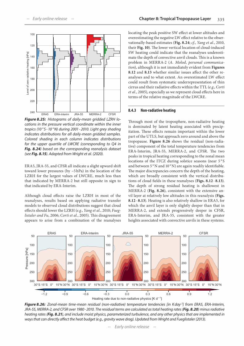
335Chapter 8: Tropical Tropopause Layer
-- Early online release --
-- Early online release --
ERA5, JRA-55, and CFSR all indicate a slight upward shift toward lower pressures (by ~5 hPa) in the location of the LZRH for the largest values of LWCRE, much less than that indicated by MERRA-2 but still opposite in sign to that indicated by ERA-Interim.
Although cloud effects raise the LZRH in most of the reanalyses, results based on applying radiative transfer models to observed cloud distributions suggest that cloud effects should lower the LZRH (e.g., Yang et al., 2010; Fueg-listaler and Fu, 2006; Corti et al., 2005). This disagreement appears to arise from a combination of the reanalyses
locating the peak positive SW effect at lower altitudes and overestimating the negative LW effect relative to the obser-vationally-based estimates (Fig. 8.24; cf., Yang et al., 2010, their Fig. 10). The lower vertical location of cloud-induced SW heating could indicate that the reanalyses underesti-mate the depth of convective anvil clouds. This is a known problem in MERRA-2 (A. Molod, personal communica-tion), although it is not immediately evident from Figures 8.12 and 8.13 whether similar issues affect the other re-analyses and to what extent. An overestimated LW effect could result from systematic underrepresentation of thin cirrus and their radiative effects within the TTL (e.g., Corti et al., 2005), especially as we represent cloud effects here in terms of the relative magnitude of the LWCRE.
8.4.3 Non-radiative heating
Through most of the troposphere, non-radiative heating is dominated by latent heating associated with precip-itation. These effects remain important within the lower part of the UTLS, but approach zero around and above the tropopause. Figure 8.26 shows the residual (non-radia-tive) component of the total temperature tendencies from ERA-Interim, JRA-55, MERRA-2, and CFSR. The two peaks in tropical heating corresponding to the zonal mean locations of the ITCZ during solstice seasons (near 5 ° S and between 5 ° N and 10 ° N) are again readily identifiable. The major discrepancies concern the depth of the heating, which are broadly consistent with the vertical distribu-tions of cloud fields in these reanalyses (Figs. 8.12 - 8.13). The depth of strong residual heating is shallowest in MERRA-2 (Fig. 8.26), consistent with the extensive an-vil layer at relatively low altitudes in this reanalysis (Figs. 8.12 - 8.13). Heating is also relatively shallow in ERA5, for which the anvil layer is only slightly deeper than that in MERRA-2, and extends progressively deeper in CFSR, ERA-Interim, and JRA-55, consistent with the greater heights associated with convective anvils in these systems.
Figure 8.25: Histograms of daily-mean gridded LZRH lo-cations in the pressure vertical coordinate within the inner tropics (10 ° S - 10 ° N) during 2001 - 2010. Light grey shading indicates distributions for all daily-mean gridded samples. Colored shading in each column indicates distributions for the upper quartile of LWCRE (corresponding to Q4 in Fig. 8.24) based on the corresponding reanalysis dataset (see Fig. 8.15). Adapted from Wright et al. (2020).
Figure 8.26: Zonal-mean time-mean residual (non-radiative) temperature tendencies [in K day-1] from ERA5, ERA-Interim, JRA-55, MERRA-2, and CFSR over 1980 - 2010. The residual terms are calculated as total heating rates (Fig. 8.20) minus radiative heating rates (Fig. 8.21), and include moist physics, parameterized turbulence, and any other physics that are implemented in ways that can directly affect the heat budget (e.g., gravity wave drag). Updated from Wright and Fueglistaler (2013).

336
-- Early online release --
SPARC Reanalysis Intercomparison Project (S-RIP) Final Report -- Early online release --
Together with cloud radiative effects, differences in these terms are an important contributor to differences in total diabatic heating in the lower TTL (Fig. 8.20): shallower latent heating coupled with enhanced cloud-top LW cool-ing creates the diabatic ‘transport barrier’ that emerges in MERRA-2 and, to a lesser extent, ERA5 and CFSR (see also discussion of MERRA by Wright and Fueglistaler, 2013).
Figure 8.27 shows zonal-mean time-mean temperature tendencies from parameterized mixing in ERA-Interim, JRA-55, MERRA-2, and CFSR (Chapter 2, Table 2.8; see also Fig. 2.4 and further discussion in Chapter 2E). Although ERA5 and ERA-Interim do not directly provide separate moist physics and vertical mixing terms, it is possible to infer turbulent mixing due to shear-flow instability from offline calculations (Flannaghan and Fueglistaler, 2011). This inferred heating due to turbulent mixing in ERA-Interim is larger than the heating due to parameterized mixing in the other reanalyses, with stronger cooling between 10 hPa and 50 hPa and stronger warming between 200 hPa and 100 hPa. However, it remains about an order of magnitude smaller than the radiative terms through most of this vertical range, and the residual term (Fig. 8.26) is evidently dominated by contributions from moist physics rather than parameterized mixing in the UT. We have not performed this calculation for ERA5.
The dipole patterns seen in ERA-Interim, CFSR, and (to a lesser extent) JRA-55 imply mixing of the upper tropo-sphere with the lower stratosphere in the inner tropics. This mixing has pronounced zonal asymmetries, and of-ten shows a maximum above the tropical Indian Ocean (see Fig. 8.60; and also Fig. A8.10). The pattern in CFSR is similar to that in ERA-Interim, but weaker in amplitude. The qualitative similarity between these two reanalyses likely arises because both models use modified versions of the LTG (Louis et al., 1982; Louis, 1979) vertical diffusion
scheme in the free atmosphere. The difference in magni-tude likely relates to how the mixing coefficient is specified in the upper troposphere. This coefficient has been report-ed to be unrealistically large above the boundary layer in ERA-Interim (Bechtold et al., 2008), while that in CFSR was reformulated specifically to mitigate extremely strong tur-bulent mixing at upper levels in NCEP-NCAR R1 (Wright and Fueglistaler, 2013; Saha et al., 2010) The pattern in JRA-55 is substantially different, with cooling at the tropopause and weak warming above, coupled with warming in the subtropical LS in both hemispheres. Heating rates due to parameterized mixing in MERRA-2 are several orders of magnitude smaller than those in the other three reanalyses, as diffusion coefficients in MERRA-2 are very small above the atmospheric boundary layer (Chapter 2, Table 2.8).
8.4.4 Key findings and recommendations
Key findings
� There are large differences among reanalysis diabatic heating products within the TTL, which are known to influence transport statistics and rates of ascent in trajec-tory simulations of cross-tropopause transport in this re-gion. Differences among reanalysis diabatic heating rates in the tropical UTLS are not limited to any one compo-nent: longwave, shortwave, and non-radiative compo-nents all show substantial discrepancies. (Section 8.4)
� Differences in radiative heating rates primarily trace back to the differences in cloud fields, but there are important discrepancies in clear-sky radiative heating as well. In many cases, these discrepancies can be ex-plained by systematic differences in composition and temperature structure. (Section 8.4.2)
Figure 8.27: Zonal-mean time-mean temperature tendencies due to parameterized turbulence, Qmix [in K day-1], in ERA-Interim, JRA-55, MERRA-2, and CFSR. The tendency terms for JRA-55, MERRA-2, and CFSR are averaged over 1980 - 2010 from archived data. (There was no turbulence term available for ERA5.) The tendency term for ERA-Interim is not archived by EC-MWF and has been estimated from an offline calculation (Flannaghan and Fueglistaler, 2011) of 6-hourly analysis tempera-tures and winds using the revised Louis scheme as detailed in the ECMWF IFS documentation, part IV. The ERA-Interim result is averaged over 2001 - 2010; results are not sensitive to the chosen period and can be taken as representative.

337Chapter 8: Tropical Tropopause Layer
-- Early online release --
-- Early online release --
� Discrepancies in heating due to parameterized turbu-lent mixing are very poorly constrained. These terms may be influential near the tropopause, especially when radiative heating rates are small, though they are typically several orders of magnitude smaller than other terms in the diabatic heat budget. (Section 8.4.3)
Key recommendations
� Given large differences in reanalysis diabatic heat-ing products and related metrics within the tropical UTLS, researchers using these fields to drive or nudge model simulations of this region should use multiple reanalyses whenever possible. (Section 8.4)
8.5 Transport
Transport through the TTL controls the entrainment of tropospheric air into the stratosphere (Highwood and Hoskins, 1998). As discussed in Section 8.4, the TTL encompasses the level of zero radiative heating, which marks the transition from negative to positive heating rates and creates a barrier for the large-scale transport into the stratosphere (Folkins et al., 1999). Above the LZRH, vertical motion balances the radiative heating ac-cording to thermal balance and air is slowly ascending (Section 8.5.3). The lower TTL is penetrated by deep con-vection which becomes increasingly rare with altitude (Liu and Zipser, 2005), while the vertical motion out-side of convective towers is weak. Quantifying transport paths across the TTL for a better understanding of the chemical composition of air entering the stratosphere is often done based on CTMs and Lagrangian models driv-en by meteorological reanalyses. Studies have focused on the stratospheric dehydration point (Bonazzola and Haynes, 2004; Fueglistaler et al., 2004) and the residence time of air through the TTL (Krüger et al., 2009). Sections 8.5.1 and 8.5.2 analyze how these two quantities are rep-resented in the different reanalysis data sets.
8.5.1 Dehydration point distribution
It has been known since Brewer’s seminal work on strato-spheric circulation that tropical tropopause temperature is the key driver of stratospheric water vapor (H2O) con-centration (Brewer, 1949). As parcels approach and pass through the cold point tropopause, condensation occurs, thereby regulating the parcel’s H2O concentration to lo-cal saturation levels (e.g., Holton and Gettelman, 2001; Fueglistaler et al., 2009a). The dehydration process thus primarily depends on the air parcel temperature history.
The details of the transport and dehydration process can be understood by performing Lagrangian trajectory sim-ulations, which track the temperature history of a large number of individual air parcels. The approach applied here is based on a forward trajectory model, following
the details described in Schoeberl and Dessler (2011), with trajectories calculated using the Bowman trajectory code (Bowman et al., 2013; Bowman, 1993). In the forward tra-jectory mode, the number of trajectories that contribute to dehydration events in a particular geographic region depend on the circulation and temperature structures of the respective reanalysis. We conduct diabatic Lagran-gian runs in isentropic coordinates. The parcel initia-tion level is chosen to be the 370 K isentrope, which is generally above the level of zero radiative heating in the tropics but below the tropical tropopause (~375 - 380 K; see Fig. 8.1). In the TTL, water vapor is conserved along the trajectories except when saturation occurs. Water va-por excess is instantaneously removed from the parcel to keep the relative humidity with respect to ice from exceeding 100 %. Along each trajectory, we define the point with the lowest temperature and minimum satu-ration mixing ratio as the final dehydration point (FDP). The FDP determines the final H2O mixing ratio of each trajectory as it enters the stratosphere and is equivalent to the Lagrangian cold point. Details of the trajectory model, the setup of the simulations and the FDP calcula-tions are given in Wang et al. (2015) and Schoeberl et al. (2013). The trajectory model is driven by meteorological reanalyses on model levels, except for CFSR where, due to availability at the time, the model was driven by data on pressure levels.
The distribution of FDP temperatures and frequencies derived from trajectory simulations driven by modern reanalyses for 2007 - 2010 are shown in Figure 8.28. The Lagrangian cold point temperatures (black and white contour lines) show strong deviations, with ERA-Inter-im having the lowest and MERRA the highest dehydra-tion temperatures among the model level data sets. Tra-jectories driven by CFSR data on pressure levels show unrealistically warm cold points consistent with the Eulerian cold point comparison (Section 8.2). Despite different background temperatures for the different re-analysis data, the dehydration patterns given by their frequency distribution agree quite well. The strongest dehydration occurs over the tropical western Pacific, South America, and Africa, where frequent deep con-vection leads to a cooling above, which results in a high-er and colder tropopause. The Asian monsoon during summertime is another important dehydration center (see Sections 8.8 and 8.8.6).
Figure 8.29 shows the evolution of the FDP distribution as a function of latitude. The largest occurrence frequen-cies migrate northward from boreal winter to summer, with the most intense dehydration occurring during the NH winter season when the tropopause is coldest. How-ever, different reanalyses demonstrate different seasonal changes in FDP frequencies. These differences are caused by the combined effects of differences in the circulation and differences in the background temperatures. For ex-ample, the run driven by ERA-Interim shows less dehy-dration events between May and August than JRA-55.

338
-- Early online release --
SPARC Reanalysis Intercomparison Project (S-RIP) Final Report -- Early online release -- -30-20-10
0102030
Latit
ude
(O )
187
188188
189
189
189
189
190 190189
189
189
189
DJF
-30-20-10
0102030
Latit
ude
(O )
189190
190
190
191
191
191
189 MAM
-30-20-10
0102030
Latit
ude
(O )
191
192192
193
193
193
193
194
194
JJA
0 60 120 180 240 300Longitude (O )
-30-20-10
0102030
Latit
ude
(O )
190191
191
191192
192
192
192
19219
2
193
SON
7 1038 5379 111851707536203
FDP Events (#)
0 60 120 180 240 300Longitude (O )
-30-20-10
0102030
Latit
ude
(O )
189
189
190 190
191
191
191
191
192
192
192
189 AL
L1 1447 150294272365210125754
FDP Events (#)
-30-20-10
0102030
Latit
ude
(O )
187
188189
189
190 190
190
190
191
189
189
DJF
-30-20-10
0102030
Latit
ude
(O )
189190
190191
191 191
192
192
189 MAM
-30-20-10
0102030
Latit
ude
(O )
191
192
193
193
193
194194195
JJA
0 60 120 180 240 300Longitude (O )
-30-20-10
0102030
Latit
ude
(O )
191
191
192
192
192
193
193
193
SON
1 883 4423 101801744035602
FDP Events (#)
0 60 120 180 240 300Longitude (O )
-30-20-10
0102030
Latit
ude
(O )
189
190
190
191
191
191
191
192
192
192193194195
189 AL
L
1 1164 129664183171741168570
FDP Events (#)
-30-20-10
0102030
Latit
ude
(O )
190
191
192
192 193
DJF
-30-20-10
0102030
Latit
ude
(O )
191192
192193
193
194
194
MAM
-30-20-10
0102030
Latit
ude
(O )
193194
194
194
195 195
195
195
195
JJA
0 60 120 180 240 300Longitude (O )
-30-20-10
0102030
Latit
ude
(O )
192193
193
193
194
194
195
195
SON
2 980 5046 101451788642344
FDP Events (#)
0 60 120 180 240 300Longitude (O )
-30-20-10
0102030
Latit
ude
(O )
191
192
19319
3
193
193
194
194194 195
ALL
2 1695 166484612175752144743
FDP Events (#)
-30-20-10
0102030
Latit
ude
(O )
187188
188
189
189
189
189
190191
189
189
189
DJF
-30-20-10
0102030
Latit
ude
(O )
189
189
190
190
190
191
191
191192
192
189
189
MAM
-30-20-10
0102030
Latit
ude
(O )
191
191
192
192
193
19319
3194
194
JJA
0 60 120 180 240 300Longitude (O )
-30-20-10
0102030
Latit
ude
(O )
190
191
191
191
192
192192
193 193
SON
6 1581 8622 211313327370622
FDP Events (#)
0 60 120 180 240 300Longitude (O )
-30-20-10
0102030
Latit
ude
(O )
189
190
190
190
191
191191
192 19
2
192193
189 AL
L
6 2553 2862585289137891240259
FDP Events (#)
-30-20-10
0102030
Latit
ude
(O )
187
188188
189190
190
190
190190
191
191189
DJF
-30-20-10
0102030
Latit
ude
(O )
189190
190
190
191
191
191
191192
192
192
189 MAM
-30-20-10
0102030
Latit
ude
(O )
192193
193
193
194195
JJA
0 60 120 180 240 300Longitude (O )
-30-20-10
0102030
Latit
ude
(O )
191
191
192
192
192
192
193193
193
SON
1 594 3518 7827 1511442113
FDP Events (#)
0 60 120 180 240 300Longitude (O )
-30-20-10
0102030
Latit
ude
(O )
190 190
191
191
192
192
192
192192 193
194
ALL
1 1418 146143573365878166805
FDP Events (#)
Traj.CFSR
Traj.ERAi Traj.JRA55
Traj.MERRATraj.MERRA2
12
34
56
78
9101112Climatological Months
-90 -60 -30 0 30 60 90Latitude
2 4505
10185
16568
32205
206528
MDP Events (#)
min max20% 40% 60% 80%
Normalized FDP Events
1 2 3 4 5 6 7 8 9 10 11 12Climatological Months
-30-20-10
0102030
Latit
ude
188189
189
190
190
191
191
192
192
193 25
631063943155595222709355092
FDP
Even
ts (#
)
1 2 3 4 5 6 7 8 9 10 11 12Climatological Months
-30-20-10
0102030
Latit
ude
191
191
192
192
19319
3194
194
195 8605366466192300264895451096
FDP
Even
ts (#
)
1 2 3 4 5 6 7 8 9 10 11 12Climatological Months
-30-20-10
0102030
Latit
ude
188189
189
190
190
191191
191
192
192
193 26520154166154560251956410763
FDP
Even
ts (#
)
1 2 3 4 5 6 7 8 9 10 11 12Climatological Months
-30-20-10
0102030
Latit
ude
188189
189
190
190
191
191
192
192
193 25644762141150796222155339762
FDP
Even
ts (#
)
1 2 3 4 5 6 7 8 9 10 11 12Climatological Months
-30-20-10
0102030
Latit
ude
188189
189
190
190
191
191
192
192
193 348825110528318102479827757730
FDP
Even
ts (#
)
Traj.CFSR
Traj.ERAi Traj.JRA55
Traj.MERRATraj.MERRA2
12
34
56
78
9101112Climatological Months
-90 -60 -30 0 30 60 90
Latitude
2 4505
10185
16568
32205
206528
MDP Events (#)
min max20% 40% 60% 80%
Normalized FDP Events
1 2 3 4 5 6 7 8 9 10 11 12Climatological Months
-30-20-10
0102030
Latit
ude
188189
189
190
190
191
191
192
192
193 25
631063943155595222709355092
FDP
Even
ts (#
)
1 2 3 4 5 6 7 8 9 10 11 12Climatological Months
-30-20-10
0102030
Latit
ude
191
191
192
192
193
193
194
194
195 8605366466192300264895451096
FDP
Even
ts (#
)
1 2 3 4 5 6 7 8 9 10 11 12Climatological Months
-30-20-10
0102030
Latit
ude
188189
189
190
190
191191
191
192
192
193 26520154166154560251956410763
FDP
Even
ts (#
)
1 2 3 4 5 6 7 8 9 10 11 12Climatological Months
-30-20-10
0102030
Latit
ude
188189
189
190
190
191
191
192
192
193 25644762141150796222155339762
FDP
Even
ts (#
)
1 2 3 4 5 6 7 8 9 10 11 12Climatological Months
-30-20-10
0102030
Latit
ude
188189
189
190
190
191
191
192
192
193 348825110528318102479827757730
FDP
Even
ts (#
)
Traj.CFSR
Traj.ERAi Traj.JRA55
Traj.MERRATraj.MERRA2
12
34
56
78
9101112Climatological Months
-90 -60 -30 0 30 60 90
Latitude
2 4505
10185
16568
32205
206528
MDP Events (#)
min max20% 40% 60% 80%
Normalized FDP Events
1 2 3 4 5 6 7 8 9 10 11 12Climatological Months
-30-20-10
0102030
Latit
ude
188189
189
19019
0191
191
192
192
193 25
631063943155595222709355092
FDP
Even
ts (#
)
1 2 3 4 5 6 7 8 9 10 11 12Climatological Months
-30-20-10
0102030
Latit
ude
191
191
192
192
193
193
194
194
195 8605366466192300264895451096
FDP
Even
ts (#
)
1 2 3 4 5 6 7 8 9 10 11 12Climatological Months
-30-20-10
0102030
Latit
ude
188189
189
190
190
191191
191
192
192
193 26520154166154560251956410763
FDP
Even
ts (#
)
1 2 3 4 5 6 7 8 9 10 11 12Climatological Months
-30-20-10
0102030
Latit
ude
188189
189
190
190
191
191
192
192
193 25644762141150796222155339762
FDP
Even
ts (#
)
1 2 3 4 5 6 7 8 9 10 11 12Climatological Months
-30-20-10
0102030
Latit
ude
188189
189
190
190
191
191
192
192
193 348825110528318102479827757730
FDP
Even
ts (#
)
Traj.CFSR
Traj.ERAi Traj.JRA55
Traj.MERRATraj.MERRA2
12
34
56
78
9101112Climatological Months
-90 -60 -30 0 30 60 90
Latitude
2 4505
10185
16568
32205
206528
MDP Events (#)
min max20% 40% 60% 80%
Normalized FDP Events
Figure 8.28: Distribution of annual mean final dehydration points (FDPs) derived from trajectory model simulations driven by different reanalyses for 2007 - 2010. For convenience of intercomparing the different reanalyses with largely varying total FDP events, we show the percentiles of the FDP event distribution. Temperatures associated with final dehydration are shown as black contours at 1 K intervals, with the 189 K isotherm highlighted in white.
Figure 8.29: Like Figure 8.28 but for the seasonal cycle of final dehydration points (FDPs).

339Chapter 8: Tropical Tropopause Layer
-- Early online release --
-- Early online release --
8.5.2 TTL residence time
One of the advantages of trajectory modeling is that it retains the his-tory of each individual parcel. For an upward moving parcel released at a fixed isentropic surface, we can examine the time the parcel takes to ascend to a specified higher is-entropic level for the first time. We refer to this as the residence time (τ) of that parcel in the layer between the two isentropic levels. Based on the trajectory runs described in Section 8.5.1, we calculate the resi-dence times for air mass transport between 370 K and 450 K according to the five reanalyses. The mean profile of residence time quantifies the speed of the upwelling branch of the Brewer-Dobson Circulation (Chapter 5). Note, however, that atmospheric mixing is not taken into account in the trajectory calculations pre-sented here, which can impact the total transport velocity and the water vapour tape recorder upwelling.
Figure 8.30a shows the residence time averaged over the tropics (30 ° N - S) starting from the 370 K level for 2005 - 2010. Only 23 - 25 days are required for newly-in-itiated parcels to ascend across the tropopause (~ 380 K). One exception is ERA-Interim, which has larger heating rates in the TTL (Wright and Fueglistaler, 2013; Wang et al., 2014; Section 8.4) and thus relatively rapid parcel ascent (only 19 days) across the tropopause. Within the TTL, par-cels stay for ~ 3 months or longer when using the MERRA, MERRA-2, or CFSR circulations, whereas parcels only stay for ~ 2 months when using the ERA-Interim or JRA-55 circulations. Below the 370 K potential temperature level, MERRA-2 diabatic heating rates are often negative and cannot be used to drive tropical upwelling simulations (see also Section 8.4). Overall, the vertical range and sea-sonality for residence time based on different reanalyses
is in qualitative agreement with previous studies on res-idence time (Ploeger et al., 2010; Krüger et al., 2009) and trace gas seasonality in the TTL (Ploeger et al., 2012). The residence time shows a seasonal dependence (Fig. 8.30b), with parcels ascending faster (slower) during boreal win-ter-spring (summer-fall), thus resulting in shorter (longer) residence times. Deviations of the seasonal cycle are most pronounced around the cold point tropopause, where the amplitude of the seasonal cycle based on JRA-55 is more than twice as large as that based on CFSR.
Figure 8.31 shows horizontal distributions of the 370 K - 380 K residence time from different trajectory runs during the boreal winter and summer seasons av-eraged over 2005 - 2010. All trajectory runs show the tropical Western Pacific and the Asian monsoon as two distinct centers of strong ascent during boreal winter and summer, respectively. Differences in residence time depend on the magnitudes of total diabatic heating rates among the different reanalyses, with broad agreement that heating rates from ERA-Interim are the largest over-all among these five reanalyses (see Section 8.4). Apart from the overall differences, the spatial distribution of the residence times also varies among the reanalyses.
[-15,0],[0,15]
0 30 60 90 120 150 180 210 240residence time (days)
370
380
390
400
410
420
430
440
450
θ (K
)
16.5
17.0
17.5
18.0
18.5
19.0
Appr
ox. A
lt (k
m)
Tropical:Lat.[-30,30]
0 30 60 90 120 150 180 210 240residence time (days)
370
380
390
400
410
420
430
440
450
θ (K
)
16.016.5
17.0
17.5
18.0
18.5
19.0
Appr
ox. A
lt (k
m)
N.Mid.Lat.[30,60]
0 30 60 90 120 150 180 210 240residence time (days)
370
380
390
400
410
420
430
440
450
θ (K
)
16.0
16.5
17.0
17.5
18.0
Appr
ox. A
lt (k
m)
N.Polar.[60,90]
0 30 60 90 120 150 180 210 240residence time (days)
370
380
390
400
410
420
430
440
450
θ (K
)
16.0
16.5
17.0
Appr
ox. A
lt (k
m)
S.Mid.Lat.[-60,-30]
0 30 60 90 120 150 180 210 240residence time (days)
370
380
390
400
410
420
430
440
450
θ (K
) 16.0
16.5
17.0
17.5
Appr
ox. A
lt (k
m)
S.Polar.[-60,-90]
0 30 60 90 120 150 180 210 240residence time (days)
370
380
390
400
410
420
430
440
450
θ (K
)
16.0
16.5
17.0
Appr
ox. A
lt (k
m)
Vertical Profile:lon[0,360],lat[-90,90],vert[368,452],time[2005.042,2015.958],X00: residence_time_161008_mthd_MER_day_sav1_h2oM_age_grid3D_monly_1979-2016.nc; X01: residence_time_161010_mthd_MER2_day_sav1_h2oM_age_grid3D_moX02: residence_time_161014_mthd_ERAi_day_sav1_h2oM_age_grid3D_monly_1979-2016.nc; X03: residence_time_161012_mthd_JRA55_day_sav1_h2oM_age_grid3D_mX04: residence_time_161016_mthd_CFSR_day_sav1_h2oM_age_grid3D_monly_1979-2010.nc;
MERRA MERRA2 ERA-Interim JRA55 NCEP-CFSR
1 2 3 4 5 6 7 8 9 10 11 12Climatological Months
182022242628 380 K
50607080
resid
ence
tim
e (d
ays)
400 K80
100120140160
JANFEBMARAPRMAYJUNJULAUGSEPOCTNOVDEC420 K
Time Series: lon[0,360],lat[-30,0,0,30],,vert[368,452],time[2005.042,2015.958],X00: residence_time_161008_mthd_MER_day_sav1_h2oM_age_grid3D_monly_1979-2016.nc; X01: residence_time_161010_mthd_MER2_day_sav1_h2oM_age_grid3D_moX02: residence_time_161014_mthd_ERAi_day_sav1_h2oM_age_grid3D_monly_1979-2016.nc; X03: residence_time_161012_mthd_JRA55_day_sav1_h2oM_age_grid3D_mX04: residence_time_161016_mthd_CFSR_day_sav1_h2oM_age_grid3D_monly_1979-2010.nc;
MERRA MERRA2 ERA-Interim JRA55 NCEP-CFSR
Traj.MERRA2Traj.MERRATraj.ERAiTraj.JRA55Traj.CFSR
24d 25d 19d 23d 23d
2.8 mon3.6 mon2.1 mon2.6 mon3.2 mon
takes
109d 133d 82d102d 119d
Initiate level
J F M A M J J A S O N DMonths
a) Tropical (30o N-S) Annual Mean b) Tropical (30o N-S) Seasonal Mean
2–3 months
Fig. 8.5.3
Figure 8.30: Tropical (30 ° N - 30 ° S) a) annual mean and b) seasonal mean residence times derived from trajectories driven by modern reanalyses in the upper TTL. All residence times are for transport from the 370 K initiation level to the specified isentropic surface.
DJF
JJA
Traj.MERRA2 Traj.MERRA Traj.ERAi Traj.JRA55 Traj.CFSR
Lon (o)
Lat (
o )La
t (o )
Lon (o) Lon (o)Lon (o)Lon (o)residence time at 380K (days)
0 60 120 180 240 300 360Lon. (O )
-60
-30
0
30
60
Lat.
(O )
0 60 120 180 240 300 360Lon. (O )
0 60 120 180 240 300 360Lon. (O )
0 60 120 180 240 300 360Lon. (O )
0 60 120 180 240 300 360Lon. (O )
380
-60
-30
0
30
60
Lat.
(O )
420
-60
-30
0
30
60
Lat.
(O )
450
-60
-30
0
30
60
Lat.
(O )
MERRA
MERRA2
ERA-Interim
JRA55
500
NCEP-CFSR
binFrac:[ 0.000, 0.050, 0.100, 0.150, 0.300, 0.650, 0.900, 1.000,], Lon-Lat: lon[0,360],lat[-60,0,0,60],,vert[370,1800],time[2005.042,2015.958],X00: residence_time_161008_mthd_MER_day_sav1_h2oM_age_grid3D_monly_1979-2016.nc; X01: residence_time_161010_mthd_MER2_day_sav1_h2oM_age_grid3D_monly_1980-2016.nc; X02: residence_time_161014_mthd_ERAi_day_sav1_h2oM_age_grid3D_monly_1979-2016.nc; X03: residence_time_161012_mthd_JRA55_day_sav1_h2oM_age_grid3D_monly_1979-2016.nc; X04: residence_time_161016_mthd_CFSR_day_sav1_h2oM_age_grid3D_monly_1979-2010.nc;
12 18 20 22 24 26 30 36 180
residence time (days)
Residence Time @ 380-K (2005-2015 ave)Fig. 8.5.4
Figure 8.31: Regional differences of residence time at 380 K (started from 370 K), driven by modern reanalyses during DJF (first row) and JJA (second row) of 2005 - 2010.

340
-- Early online release --
SPARC Reanalysis Intercomparison Project (S-RIP) Final Report -- Early online release --
One of the most apparent differences is that ERA-Interim shows a much weaker equator-to-subtropics gradient in residence time during JJA than any other reanalysis con-sidered here.
Generally, all runs produce clear annual cycles of residence time as shown in Figure 8.30b, although the details dif-fer. Figure 8.32 compares interanual anomalies derived by substracting the annual cycle of tropical residence times at 380 K and 420 K during 1980 - 2015. Examined in anomaly space, all runs yield similar interannual variability of resi-dence time, mostly characterized by short-term fluctuations with no apparent long-term changes. This is consistent with the study by Krüger et al. (2009), who found a significant anticorrelation of TTL residence time with planetary wave driving in the extratropical lower stratosphere. Larger fluc-tuations are evident in the run driven by CFSR, which has distinct maxima in some years. These maxima probably re-sult from artefacts of the stream transitions which started
on 1 January in 1987, 1995, and 2010 and on 1 April in 1999 and 2005. Sudden drops in the CFSR heating rates in the lower stratosphere (~83 hPa) occur in 1987, 1990, 1995, 1999, 2005, and 2010, consistent with the signal in the residence time shown here. While cold point temperature anomalies show step like improvements in inter-reanalysis agreement around 1998 - 1999 and 2006, the same is not true for the residence time. This result demonstrates that vertical trans-port driven by diabatic heating rates is less impacted by changes in the assimilated observational data sets. Note, however that this conclusion is limited to the TTL (substan-tial discontinuities in heating rates appear at higher alti-tudes around the TOVS-ATOVS transition; see, e.g., Abalos et al., 2015) and does not mean that heating rates should be considered reliable in this region. Indeed, heating rates in the TTL based on different atmospheric reanalyses show substantial disagreements in both climatology (Section 8.4; see also Wright and Fueglistaler, 2013) and trends (e.g., Linz et al., 2019).
1980 1985 1990 1995 2000 2005 2010 2015Time
-6-4-202468
resi
denc
e tim
e An
om. (
days
)
380 K
-200
2040
resi
denc
e tim
e An
om. (
days
)1980 1985 1990 1995 2000 2005 2010 2015
420 K
Time Series: lon[0,360],lat[-30,0,0,30],,vert[368,452],time[1980.042,2015.958],X00: residence_time_161008_mthd_MER_day_sav1_h2oM_age_grid3D_monly_1979-2016.nc; X01: residence_time_161010_mthd_MER2_day_sav1_h2oM_age_grid3D_moX02: residence_time_161014_mthd_ERAi_day_sav1_h2oM_age_grid3D_monly_1979-2016.nc; X03: residence_time_161012_mthd_JRA55_day_sav1_h2oM_age_grid3D_mX04: residence_time_161016_mthd_CFSR_day_sav1_h2oM_age_grid3D_monly_1979-2010.nc;
MERRA MERRA2 ERA-Interim JRA55 NCEP-CFSR
Res
iden
ce ti
me
anom
aly
(day
s) Traj.MERRA2 Traj.MERRA Traj.ERAi Traj.JRA55 Traj.CFSR
Figure 8.32: Tropical (30 ° N - 30 ° S) residence time anomalies (by removing annual cycle) at 380 K and 420 K (both started from 370 K), for 1980 - 2015 derived from trajectories driven by modern reanalyses. CFSR only extends to 2010.
MERRA-2
-30 -15 0 15 30300
250
200
150
100
50
342
350
380
450 zERA-Interim
342
350
380
450
JRA-55
342
350
380
450
CFSR
342
350
380
450
300
250
200
150
100
50
-30 -15 0 15 30
-1.5 -1.2 -0.9 -0.6 -0.3 0 0.3 0.6 0.9 1.2 1.5
300
250
200
150
100
50
-30 -15 0 15 30300
250
200
150
100
50
-30 -15 0 15 30
Pres
sure
[hPa
]
Adiabatic cooling [K d ]-1
Figure 8.33: Upper panels: annual mean adiabatic temperature tendencies due to vertical advection by w*. Lower panels: annual mean total diabatic temperature tendencies diagnosed from analyzed winds and temperatures as described by Martineau et al. (2018).

341Chapter 8: Tropical Tropopause Layer
-- Early online release --
-- Early online release --
8.5.3 TTL tropical upwelling
The residual mean upwelling in the Brewer-Dobson Circulation leads to adiabatic cooling in the tropics (see Chapter 5). Adiaba-tic cooling then leads in turn to radiatively-driven diabatic heat-ing that pulls temperatures back toward radiative equilibrium. In principle, we expect in the TTL an approximate balance between di-abatic heating and adiabatic cool-ing in the climatological mean. Near the bottom of the TTL, latent heating may contribute to diabatic heating, while clouds may impact the radiation budget up to the cold point (see also Sect. 8.4). Figure 8.33 compares diabatic and adiabatic contributions to the temperature budget in the TTL for the climatological zonal mean in order to investigate if they balance each other out as expected. Here, the diabatic component represents the total heating rate diagnosed using the zonal-mean thermody-namic equation as described by Martineau et al. (2018). The term represents the sum of the time rate of change, meridi-onal advection, vertical advection, meridional eddy, and ver-tical eddy terms. The adiabatic cooling represents the vertical advection tendency due to the residual mean vertical velocity ( ) and is obtained as minus times the vertical temper-ature gradient.
The overall structure and magnitudes of heating and cooling patterns between the deep tropics and the subtropics confirm the approximate balance mentioned above. The strongest ad-iabatic cooling / diabatic heating arises near the top of deep convection embedded in the ITCZ (between 5 - 10 ° N and 300 - 250 hPa). There are also signatures of the double peak in tropical upwelling in the lowermost stratosphere with maxima in adiabatic cooling near 15 ° N/S (Ming et al., 2016). ERA-Interim and JRA-55 show similar double peak struc-tures in the diabatic heating fields, which are weaker and shifted to slightly higher altitudes in MERRA-2 and CFSR. Moreover, MERRA-2 shows diabatic cooling at 200 hPa. This feature is less pronounced than in diabatic heating rates based on parameterized physics (Fig. 8.20), but it is neither balanced by adiabatic warming in this region nor present in the other reanalyses. This indicates that other contributions to the heat budget are important in this region in MERRA-2. Data assimilation plays a key role in the difference between the physical temperature tendencies shown in Figure 8.20 and the diagnosed heating rates shown in Figure 8.33. How-ever, for MERRA-2 in the tropics, the influence of data as-similation is on average negative below 200 hPa and positive above 200 hPa (Fig. A8.6, Appendix A), leaving temperature tendencies at the 200 hPa level largely unaffected.
Overall, both adiabatic and diabatic tendencies are more consistent in the lower stratosphere than in the upper
troposphere. Figure 8.34 further shows that this consist-ency is not present among older reanalyses (cf., the dashed lines showing a large range of adiabatic cooling values in the lower stratosphere). Amongst the more recent products, MERRA-2 consistently shows the smallest tendencies. JRA-55’s AMIP version roughly agrees with JRA-55, although it shows somewhat smaller values throughout the profile. ERA-20C is also consistently biased towards smaller values compared to ERA-Interim.
8.5.4 Key findings and recommendations
Key findings
� Lagrangian transport studies demonstrate large differ-ences in reanalysis temperatures at the dehydration point, however, the data sets agree on the spatial distribution of dehydration locations. Given warm biases at the Eulerian cold point tropopause, Lagrangian dehydration points can be expected to be up to 1 K too warm. (Section 8.5.1)
� Diabatic vertical ascent appears to be faster in ERA-In-terim, which produces a TTL residence time (between 370 K and 400 K) of ~2 months, in contrast to residence times of ~3 months or longer based on MERRA, MER-RA-2, or CFSR. Despite the large differences in absolute values, all reanalysis data sets produce roughly similar distributions, seasonal cycles, and interannual varia-tions of TTL residence time. (Section 8.5.2)
Key recommendations
� Lagrangian studies above 370 K (120 hPa), based on diabatic trajectories show more realistic tropical as-cent rates when based on MERRA-2 or CFSR. Below 370 K (120 hPa), however, diabatic heating rates in these two data sets imply time-mean descent and therefore require careful treatment of convective detrainment source terms. (Section 8.5; see also 8.4 and 8.8)
Figure 8.34: Tropical (20 ° S – 20 ° N) mean adiabatic temperature tendencies due to verti-cal advection by for DJF (left) and JJA (right). MERRA-2, ERA-Interim, ERA5, JRA-55 and CFSR are shown as solid lines, MERRA, ERA-40, JRA-25, NCEP-NCAR R1, and NCEP-DOE R2 as dashed lines and JRA-55 AMIP, 20CRv2c and ERA-20C as dotted lines.
-1.2 -1.0 -0.8 -0.6 -0.4 -0.2 -0.0
100
DJF adiabatic tendency, [20S,20N]
-1.2 -1.0 -0.8 -0.6 -0.4 -0.2 -0.0temperature tendency (K/day)
300
200
150
100
70
50
pres
sure
(hPa
)-1.2 -1.0 -0.8 -0.6 -0.4 -0.2 -0.0
100
MERRA-2MERRAERA-InterimERA5ERA-40JRA-55JRA-55AMIPJRA-25NCEP-NCAR R1NCEP-DOE R220CRv2cERA-20CCFSR
JJA adiabatic tendency, [20S,20N]
-1.2 -1.0 -0.8 -0.6 -0.4 -0.2 -0.0temperature tendency (K/day)
300
200
150
100
70
50

342
-- Early online release --
SPARC Reanalysis Intercomparison Project (S-RIP) Final Report -- Early online release --
Figure 8.35: Longitude-latitude sections of the climatological temperature anomaly at 100 hPa during (left) June - August and (right) December - February 1979 - 2005, derived from (top to bottom) MERRA, 20CR v2, NCEP-NCAR R1, NCEP-DOE R2, CFSR, ERA-40, ERA-Interim, JRA-25, JRA-55, and JRA-55AMIP reanalysis datasets. The anomaly is calculated from the tropical mean value (10 ° S - 10 ° N) in each season. Values of the minimum temperature anomaly and the minimum HSI-1 are shown in the legend of each panel. Observed climatological OLR is also shown as white contours (for 180, 200, and 220 W m-2).

343Chapter 8: Tropical Tropopause Layer
-- Early online release --
-- Early online release --
8.6 Wave activity
Tropical convective activity has unique horizontal patterns in different seasons and sub-seasonal variability, resulting in variabilities in tropical tropopause temperature at these spatio-temporal scales through equatorial wave dynamics. These variabilities strongly influence transport and de-hydration in the TTL. In this section, we discuss tropical 100 hPa wave activity at seasonal and sub-seasonal time scales in temperature and winds in multiple reanalyses. (See Chapter 9 for equatorial wave activities at higher altitudes.)
8.6.1 Horseshoe-shaped structure at the 100 hPa temperature
Low temperatures at 100 hPa generally occur over the equa-tor in the eastern hemisphere and extend northwestward and southwestward to form a horseshoe-shaped structure (e.g., Highwood and Hoskins, 1998). This structure resembles a the-oretical stationary wave response known as the Matsuno-Gill pattern (Gill 1980; Matsuno, 1966), which is a superposition of the Rossby and Kelvin wave responses to tropical convective heating. The magnitude of the 100 hPa temperature anoma-lies is different among reanalyses, although the climatolog-ical anomaly patterns have common features, including the horseshoe-shaped structure (e.g., Fujiwara et al., 2012).
Figure 8.35 shows the horizontal distributions of the temper-ature anomalies at 100 hPa in JJA and in DJF from 10 rea-nalysis datasets. The values for each season are climatological averages over 27 years (1979 - 2005). Active convective regions based on NOAA OLR data are also shown. In JJA, off-equato-rial strong heating in the Asian monsoon region in combina-tion with equatorial heating around the maritime continent results in a horseshoe-shaped structure in the 100 hPa tem-perature, which is equatorially asymmetric. In DJF, equato-rial heating around the maritime continent and western Pa-cific results in a dominant Kelvin wave response. Note that in individual months and years the Rossby wave response can be observed as well causing the horseshoe-shaped signal dur-ing these time periods (e.g., Fig. 1 of Nishimoto and Shiotani, 2012). Negative temperature anomalies show larger magni-tude in MERRA, 20CR v2, NCEP-NCAR R1, NCEP-DOE R2, and CFSR than in ERA-40, ERA-Interim, JRA-25, JRA-55, and JRA-55AMIP, in both seasons. In addition, positive temperature anomalies located around 60 ° E in the northern summer, which are surrounded by the negative anomalies, have larger amplitudes in MERRA, 20CR v2, and CFSR.
In order to investigate the longitudinal and seasonal vari-ations of the horseshoe shaped temperature structure in a more quantitative way, Nishimoto and Shiotani (2012) defined the index (HSI-1) from two preliminary indices, which represent the Rossby and Kelvin wave responses.
Figure 8.36: Longitude-time sections of climatological HSI-1 derived from MERRA, 20CR v2, NCEP-NCAR R1, NCEP-DOE R2, CFSR, ERA-40, ERA-Interim, JRA-25, JRA-55, and JRA-55AMIP reanalysis datasets and climatological NOAA/OLR averaged over 15 ° S - 20 °N .

344
-- Early online release --
SPARC Reanalysis Intercomparison Project (S-RIP) Final Report -- Early online release --
As representation of the Rossby response, the index HSI-R is defined as the meridional curvature of the 100 hPa temper-ature at the equator as a function of longitude x and time t:
(8.4),
where denotes the temperature at the equator, and and are the temperatures averaged over 10 ° N - 15 ° N and 10 ° S - 15 ° S, respectively. If low temperatures occur in the 10 ° - 15 ° latitude bins as the Rossby response, the HSI-R in-dex becomes negative.As a representation of the Kelvin re-sponse, the index HSI-K is defined as the zonal gradient of the 100 hPa temperature along the equator:
(8.5),
where a differentiation length is set at 20 ° longitude. When the temperature structure represents the Kelvin response, the HSI-K index becomes negative.
As the HSI-R and HSI-K values change accordingly with a positive correlation in response to heating generated by con-vection, the index HSI-1 is defined by using the first compo-nent of the empirical orthogonal function analysis of HSI-R and HSI-K values:
(8.6).
In the horseshoe-shaped structure, negative values of HSI-K are located slightly to the east of the negative values of HSI-R in agreement with the Matsuno-Gill pattern, so that we set the longitudinal phase lag of HSI-K relative to HSI-R at α = +15 °. The coefficients a = 0.504 and b = 0.864 are derived from the monthly mean composite data of MERRA, ERA-In-terim, JRA-55, and CFSR. In this section, we apply the HSI-1 index to 9 reanalyses and compare the results quantitatively.
Longitude-time sections of climatological monthly HSI-1 values and climatological monthly NOAA/OLR (as a proxy for convective activity) values averaged over 15 ° S - 20 ° N are provided in Figure 8.36. The seasonal variation is almost identical among the reanalyses, and negative HSI-1 values
exist in the eastern hemisphere with peaks in the northern and southern summer seasons. During NH summer, the negative HSI-1 values extend from 40 °E - 150 °E in every reanalysis and the peak is located between 60 ° E - 100 ° E in July or August. The amplitude of the negative HSI-1 values is very large in MERRA, 20CR v2, and CFSR corresponding to the large positive temperature anomalies located around 60 ° E as shown in Figure 8.35. During SH summer, the neg-ative values extend over 60 ° E - 150 ° E in MERRA, 20CR v2, NCEP-NCAR R1, NCEP-DOE R2, and CFSR, whereas those in ERA-40, ERA-Interim, JRA-25, JRA-55, and JRA-55AMIP extend narrower in longitude (80 ° E - 150 ° E).
As Nishimoto and Shiotani (2012) showed based on monthly mean ERA40 data, the seasonal cycle of negative HSI-1 values is significantly related to that observed in convective activities over three monsoon regions: the South Asian Summer Mon-soon and the North Pacific monsoon areas during the north-ern summer and the Australian monsoon area during the southern summer. This relationship is expected theoretically because the Matsuno-Gill pattern is the response from trop-ical heating including off-equatorial heating within the trop-ics (Gill, 1980). The correlation coefficient between the clima-tological monthly HSI-1 values averaged over 40 ° E - 150 ° E and the OLR values averaged over 60 ° E - 180 ° E is larger than 0.8 for every reanalysis dataset and statistically significant.
Figure 8.37 shows a scatter plot of the climatological HSI-1 value averaged over 60 ° E - 120 ° E and the climatologi-cal temperature anomaly averaged over 10 ° S - 10 ° N and 90 ° E - 180 ° E among various datasets. Among the reanalysis datasets, a positive relationship is found between the clima-tological HSI-1 value and the climatological temperature anomaly. The HSI-1 value ranges from -1.3 to -0.6 while the temperature anomaly ranges from -1.6 K to -0.7 K. The data-sets can be divided into two groups depending on whether the HSI-1 value is smaller or larger than - 1.0. The former group with the smaller HSI-1 values includes MERRA (a), 20CR v2 (b), and the NCEP series (c1-c3) of reanalyses, while the latter group includes the ECMWF (d1-d2) and JRA series (e1-e2) of reanalyses. These results suggest that the strength of the horseshoe-shaped structure, which controls the magnitude of cold temperature anomaly, is dependent on the inherent dynamical model or assimilation system used in reanalysis.
8.6.2 Equatorial waves
Significant sub-seasonal variability is found in temperature, horizontal winds, and other parameters in the TTL (Fueglis-taler et al., 2009a). This is due to various types of equatorial waves, intraseasonal oscillations/the Madden-Julian Oscil-lation (MJO) (Madden and Julian, 1994), and other distur-bances that are primarily generated by tropical organized convection (e.g., Kiladis et al., 2009). Previous case studies have investigated the roles of equatorial Kelvin waves in the TTL for large temperature changes, ozone transport, dehydration, turbulence generation, and cirrus variations (see, e.g., Fujiwara et al., 2012 and the references therein).
Figure 8.37: Scatter plot of the climatological HSI-1 averaged over 60 ° E - 120 ° E vs. the climatological temperature anomaly averaged over 10 ° S - 10 ° N and 90 °E - 180 °E. The composite (*) is made from MERRA, ERA-Interim, JRA-55, and CFSR.

345Chapter 8: Tropical Tropopause Layer
-- Early online release --
-- Early online release --
In this Section, we discuss the wave ac-tivity at the 100 hPa level using various reanalysis data sets. The data used are sub-daily (3-hourly for MERRA and MERRA-2; 6-hourly for the other rea-nalyses). Characteristics of equatorial waves for different stratospheric levels can also be found in Section 9.3 and Kim et al. (2019) using the same method as described here.
The method of obtaining the wave ac-tivity is based on the zonal wavenum-ber–frequency (k - ω) spectral analy-sis with equatorially symmetric and antisymmetric decomposition with a background spectrum estimation. The power spectral densities (PSDs) of the symmetric and antisymmetric com-ponents of variables (e.g., for temper-ature, and
, respec-tively) are calculated as a function of k and ω for each month, after applying a 90-day window centered on the month (see Kim et al., 2019, for further de-tails). The PSDs are then averaged over 15 ° N - 15 ° S. The background spectra of the symmetric and antisymmetric components each are obtained fol-lowing Fujiwara et al. (2012), by iter-ating 1-2-1 running average 23 times along the zonal wavenumbers and 7 times along the frequencies. The PSDs are presented in the variance-pre-serving form with log-scale axes, i.e.,
, where F is the Fourier coefficient of the symmetric or an-tisymmetric component windowed, and the spectral inter-vals ∆k and ∆ω are 1 and 1/90 cyc day-1, respectively.
Figure 8.38 shows the PSDs of 100 hPa temperature aver-aged over 1981 - 2010, obtained using ERA-Interim, MERRA, MERRA-2, CFSR, JRA-55, and JRA-55C. The symmetric and antisymmetric spectra are shown for k > 0 and k < 0, respec-tively. In the symmetric PSDs, the spectra from the six rea-nalyses have a similar shape: the primary peak is at k = 2 and ω = 0.09 - 0.1 cyc day-1, and a large portion of the PSD around this peak appears between the dispersion curves of Kelvin waves for the vertical wavelengths (Lz) of 2.5 km and 10 km. These curves also correspond to the zonal phase speeds of about 9.5 m s-1 and 38.2 m s-1, respectively. The peak PSD val-ue is largest in ERA-I (1.64 K2) among the reanalyses, while the PSD at low phase speeds (around the dispersion curve of Lz = 2.5 km) is larger in MERRA-2 than in the others. A sec-ondary peak appears at k = 2 and ω ~ 0.02 cyc day-1 (~50-day period), which is associated with the MJO.
In the antisymmetric PSDs (Fig. 8.38b), a large portion of the
PSD appears around the dispersion curves of mixed Ross-by-gravity (MRG) waves for Lz of 2 - 8 km, with a peak at k = 5 and ω = 0.17 - 0.18 cyc day-1. The PSD values in MERRA-2 are largest in most spectral regions among the reanalyses. A sig-nificant portion of the PSD is also distributed in low-frequen-cy ranges (ω < 0.1 cyc day-1). This can be due to the westerly background wind in the western hemisphere where the dis-persion curves might shift to low-frequency ranges. Consist-ent to this, the low-frequency wave activity is concentrated on the western hemisphere (Fig. S2 of Kim et al., 2019). It can also be attributed to the co-existence of free Rossby modes (e.g., Fujiwara et al., 2012; Madden, 2007).
Figure 8.39 shows the wave activity (see Fujiwara et al. (2012), for the definition of the wave activity) obtained using 100 hPa datasets from the six reanalyses (left six columns). In addition, the wave activity calculated at the native model levels and interpolated to 100 hPa is also shown (rightmost four columns). In comparison of the model-level results, it is found that the ERA-In-terim presents the largest Kelvin and MRG wave ac-tivity for temperature and vertical-wind components.
Figure 8.38: Zonal wavenumber–frequency power spectra of 100 hPa tem-perature for the (a) symmetric and (b) antisymmetric components averaged over 15 ° N - 15 ° S for 1981 -2 010 obtained using ERA-Interim, MERRA, MERRA-2, CFSR, JRA-55, and JRA-55C, along with the dispersion curves of Kelvin waves for the verti-cal wavelengths of 2.5, 5, and 10 km assuming windless background states (black solid) in (a) and those of mixed Rossby-gravity waves for 2, 4, and 8 km (black dot-ted) in (b). The ratios to the symmetric and antisymmetric background spectra are also indicated in (a) and (b), respectively, for the values of 1.1, 1.5, and 2 (white solid). The symmetric and antisymmetric spectra are shown only for positive and negative zonal wavenumbers, respectively. (Modified after Kim et al., 2019; see also Fig. 9.30).

346
-- Early online release --
SPARC Reanalysis Intercomparison Project (S-RIP) Final Report -- Early online release --
On the other hand, the zonal-wind component of the wave activity is largest in MERRA-2. JRA-55 presents a moderate amount of the wave activity. The wave activi-ty in JRA-55C is smaller than that in JRA-55, as expect-ed, because of absence of the satellite data assimilation. The difference between the two is roughly 15 - 20 %. The wave activity calculated using the 100 hPa datasets is al-ways smaller than that using the model-level datasets, by approximately 20 - 30 % for ERA-Interim, JRA-55, and JRA-55C. The underestimation is much less for MER-RA-2 (and also MERRA, not shown) because they have a model level that is very close to 100 hPa (see Appendix of Chapter 2).
Fujiwara et al. (2012) made a similar spectral analysis us-ing seven reanalysis data sets (NCEP-1, NCEP-2, ERA40, ERA-Interim, JRA-25, MERRA, and CFSR) for temper-ature and horizontal winds at 100 hPa for the period of 1990 - 2000. Their results for ERA-Interim, MERRA, and CFSR are mostly consistent with the ones shown in Fig-ures 8.38 and 8.39. The older-generation reanalyses that are not included in Figures 8.38 and 8.39 show generally lower wave activity. The increase in the wave activity in recent reanalyses could result from many factors includ-ing the increase in assimilated data sets and advance of assimilation schemes as well as model vertical resolu-tions of the reanalyses. Recent numerical modeling stud-ies have reported that representation of the equatorial Kelvin and MRG waves is highly sensitive to the vertical resolution of models (e.g., Richter et al., 2014).
It was reported that the difference in the Kelvin wave variance at 100 hPa between JRA-55 and JRA-55C is per-sistently larger after the late 1990s than before (Kim et al., 2019, Fig. 7), indicating a change in the contribu-tion of satellite data to the reanalysis representation of Kelvin waves. Giv-en the timing, it is attributed to the TOVS–ATOVS transition from 1998 (see Chapter 2, Section 2.4). While the introduction of new observational instruments generally improves the quality of reanalyses, it may require users of reanalyses to be cautious when they utilize the data for study on long-term variations. For example, the temperature variance of 100 hPa Kel-vin waves exhibits a long-term trend from the mid-1990s to 2010 common-ly in ERA-Interim, MERRA, MER-RA-2, CFSR, and JRA-55, but such a trend is not clear in JRA-55C (Kim et al., 2019). The different result between JRA-55C and JRA-55 manifests an artifact in the trend estimate via the transition of the satellite instruments.
8.6.3 Key findings
� Temperature anomaly patterns at 100 hPa have common features in all reanalyses, including characteristic horse-shoe-shaped structures that resemble the stationary wave response to tropical heating. The strength of this struc-ture differs among the reanalyses depending on the as-pects of the dynamical model and/or assimilation system. Seasonal variations in the horseshoe-shaped temperature structure are almost identical among reanalyses, with a well-established horseshoe-shaped pattern during north-ern summer. (Section 8.6.1)
� The spectral shapes of low-frequency equatorial waves at 100 hPa are similar among the reanalyses, but their spec-tral magnitudes differ. Equatorial wave activity tends to be larger in ERA-Interim than in other reanalyses for most variables analyzed. JRA-55C exhibits significantly weaker wave activity than JRA-55 for both Kelvin and mixed Rossby-gravity waves, emphasizing the impact of assimilating satellite observations. (Section 8.6.2)
8.7 Width of the TTL
This Section focuses on the changes of the width of the TTL, whereas Chapter 7 includes basic evaluations of the subtropical jets and tropopause breaks. Multidiagnostic intercomparisons for changes of the tropical belt have been carried out before based on various reanalyses (see Davis and Rosenlof, 2012).
Figure 8.39: The wave activity normalized by the ensemble average for the model-level results of ERA-Interim, MERRA-2, CFSR, and JRA-55: (upper) Kel-vin waves and (lower) mixed Rossby-gravity (MRG) waves, obtained using temperature (red), zonal wind (blue), meridional wind (sky blue), and ver-tical wind (green). The first six columns present the results using standard pressure-level data, and the remaining using model-level data. See the text for the definition of the activity.

347Chapter 8: Tropical Tropopause Layer
-- Early online release --
-- Early online release --
The tropical belt has generally been defined as the region strad-dling the equator that encom-passes both the upwelling and subsiding branches of the Had-ley cells (e.g., Birner et al. 2014). A number of studies have identi-fied evidence that the latitudinal extent of the tropical belt and other features of Earth’s atmos-pheric circulation have expand-ed poleward over the last several decades (e.g., Lucas et al., 2014 and Seidel et al., 2008). This phe-nomenon has often been referred to as tropical widening.
The Hadley cell and subtropical jet both provide the physical un-derpinning for defining a tropical edge latitude. In practice, how-ever, there have been numerous definitions of the tropical edges based on atmospheric phenom-ena that are assumed to be tied to the Hadley cell or subtropical jet, such as the subtropical break in the height of the tropopause (e.g., Davis and Rosenlof, 2012). These disparate definitions of the tropical belt edges have been at least part of the reason that tropical wid-ening estimates span such a large range of values, from statistically insignificant and near zero, to several de-grees latitude per decade of highly statistically signifi-cant poleward movement.
Using climate model simulations and reanalyses, sever-al recent studies have documented the degree to which tropical edge metrics are temporally correlated with one another (Waugh et al., 2018; Davis and Birner, 2017; Sol-omon et al., 2016). These studies have identified a subset of metrics that are directly correlated with the Hadley cell extent, and another subset of metrics uncorrelated or only weakly correlated with the Hadley cell extent. The latter subset, which includes the subtropical jet (STJ) and tropopause break (TPB) metrics (Fig. 8.40), is analyzed in this chapter since these metrics are a more direct measure of the edges of the TTL.
For both types of metrics, we analyze methodologies based on instantaneous longitudinally resolved and zonal-mean annual-mean fields. The instantaneous methodology for the STJ comes from Manney and Heg-glin (2018) (Section 8.7.1), while the zonal-mean STJ methodology is from Davis and Birner (2017) (Section 8.7.3). For the tropopause break, we use the instanta-neous analysis from Martin et al. (2019) (Section 8.7.2), and the zonal-mean methodology from (Adam et al., 2018) (Section 8.7.3).
8.7.1 Zonally-resolved subtropical jet diagnostic
The locations and characteristics of the upper tropospheric jet and tropopause are determined using the JETPAC (JEt and Tropopause Products for Analysis and Characteriza-tion) package, as described by Manney et al. (2011, 2014, 2017) and Manney and Hegglin (2018). The subtropical jet latitude, altitude, and frequency, among other diagnostics, are presented in Chapter 7 “ExUTLS”. An upper tropospher-ic jet is identified wherever there is a wind speed maximum greater than 40 m s-1. The boundaries of the jet region are the points surrounding that maximum with wind speed below 30 m s-1. When more than one maximum above 40 m/s ap-pears within a given 30 m s-1 contour, they are defined as sep-arate cores if the latitude distance between them is greater than 15 degrees or the decrease in wind speed between them is greater than 25 m s-1. Since the human eye excels at this sort of pattern recognition, these parameters were tuned to approximate the choices made by visual inspection.
The lapse rate tropopause is defined using the WMO definition (Section 8.2; a review of issues related to definition of the ther-mal tropopause is given by Homeyer et al. 2010). As in Manney and Hegglin (2018), the subtropical jet is defined as the most equatorward westerly jet for which the WMO tropopause alti-tude at the equatorward edge of the jet is greater than 13.0 km and that tropopause altitude drops by at least 2.0 km from the equatorward to the poleward side of the jet. This definition identifies the jet across which the “tropopause break” occurs.
Figure 8.40: The zonal-mean general circulation for February 2000 from the MERRA-2 reanalysis: (top panel) outgoing longwave radiation; (middle panel) zonal-mean zonal wind (shading, every 5 m s-1) with tropopause pressure (black contour), mean meridional streamfunction (white contours, negative values dashed, every 20x109 kg s-1, zero-contour dotted), tropopause break (TPB) and subtropical jet (STJ) metrics; and (bottom panel) the STJ metric field given by the 400 - 100 hPa average zonal-mean zonal wind with the surface zonal-mean zonal wind subtracted.

348
-- Early online release --
SPARC Reanalysis Intercomparison Project (S-RIP) Final Report -- Early online release --
A jet intercomparison with respect to the tropical circulation is presented in Manney et al. (2017). The authors compared upper tropospheric jets (as well as multiple tropopauses and subvortex jets) in MERRA-2 with those in MERRA, ERA-In-terim, JRA-55, and CFSR. Their results show (their Figure 7) stronger Walker circulation westerlies in DJF downstream of the Australian Monsoon, and stronger easterlies associated with that monsoon. Likewise, in JJA, the jets bounding the South Asian Summer Monsoon (SASM), particularly the tropical easterly jet, are stronger / more persistent in MER-RA-2 and MERRA than in the other reanalyses studied. The Asian monsoon easterlies peak at a lower altitude in CFSR than in the other reanalyses studied (their Figure 8). Over-all, Manney et al. (2017) emphasized that not only the vertical grid spacing, but also differences in the location of the model
levels, are important in the reanalyses’ representation of jets, including the jets associated with tropical circulations.
Jet latitudes and corresponding latitude shifts are ex-amined based on JETPAC products for the time period 1980 - 2014 in Manney and Hegglin (2018). Their analysis is based on identification of individual jets, thus separat-ing the subtropical and polar jets, and highlights the large regional and seasonal variation in trends in jet location. Therefore, the results sometimes reveal different trends in tropical width than have been shown using zonal or annual mean diagnostics or diagnostics that do not clearly separate the subtropical and polar jets (Manney and Hegglin, 2018). A brief summary of the results for subtropical jet latitudes, which are used as a measure of tropical width, is given below.
Figure 8.41: Bar charts of global subtropical jet latitude and NH/SH subtropical jet separation as a function of month, season, and annual, showing five reanalyses. The bars show the slopes of the linear fits and the error bars (centered about the top of the bars) the 1-sigma uncertainty in those slopes. Note that, in this and similar figures, absolute value of lati-tude is used, so positive slopes (bars extending upward from the zero line) indicate a poleward shift in both hemispheres. Triangles indicate cases where the permutation analysis shows the slope to be significant at the 95 % confidence level. Adapted from Manney and Hegglin (2018).
Figure 8.42: As in Fig. 8.41, but as a function of longitude during DJF. Adapted from Manney and Hegglin (2018).

349Chapter 8: Tropical Tropopause Layer
-- Early online release --
-- Early online release --
Subtropical jet latitude changes are shown in Fig-ure 8.41 including the slopes, and ± 1-σ uncertain-ties from each reanalysis for all months and seasons and annually. Annually, and during some seasons (DJF and MAM) and months (e.g., January to March in both hemispheres) the reanalyses do not agree on the sign of the latitude change over 1980 through 2014. Robust (and sometimes significant) latitude increases are seen in June through October in both hemispheres, and robust NH latitude decreases in November and Decem-ber. While the sign of these changes agrees among the reanalyses, the magnitude varies strongly.
Longitudinal variations of the jet latitude changes are shown in Figure 8.42 with DJF from Figure 8.41 broken down into 20 ° longitude regions. Robust positive shifts are seen in the NH over Europe and Asia, in the region where a strong, nearly zonal subtropical jet dominates the flow (e.g., Manney et al., 2014). Negative shifts are seen in the eastern Pacific in both hemispheres, and over South America and the western Atlantic in the SH, but the magnitude of the SH shifts varies greatly between the reanalyses, and CFSR shows positive shifts in part of this region. These changes thus result in inconsistent changes in tropical width in DJF, except for clear tropical narrowing over the eastern Pacific.
Regions and seasons that show robust changes in tropical width are summarized in Figure 8.43, where boxes are filled only if the trends of all four reanalyses agree in sign and the individual reanalysis’s trend is greater than the 1-σ uncertainty. As discussed by Manney and Hegglin (2018), the most robust changes are where all reanalyses agree on the sign of the trend, the slope is greater in magnitude than the 1-σ uncertainty, and the permutation analysis shows significance at the 95 % confidence level. Such robust chang-es in tropical width are seen only in a few regions and sea-sons: robust tropical widening occurs in JJA over Africa and parts of Asia, and in SON over the western Pacific; robust tropical narrowing occurs in DJF over the eastern Pacific and in MAM over the Atlantic and western Africa. Because
these jet-based diagnostics cannot be compared with obser-vations, the agreement among the reanalyses was used as a key factor in assessing the robustness of trends.
8.7.2 Zonally-resolved tropopause break diagnostic
The so-called tropopause break (i.e., the sharp discontinu-ity in tropopause altitude between the tropics and extrat-ropics) is used as an instantaneous metric for the northern and southern edges of the tropics. To identify tropopause break latitudes, lapse-rate (WMO) tropopause altitudes are computed at each analysis time using model-level temper-ature and geopotential height fields from each reanalysis. Following tropopause calculation, frequency distributions of tropopause altitudes are computed for each hemisphere to enable identification of the frequency minimum be-tween the high-altitude tropical mode and the low-altitude extratropical mode. The tropopause height corresponding to the frequency minimum in each hemisphere is then used as a threshold for global contouring, which provides the instantaneous latitude of the tropopause break as a function of longitude. Additional detail on this process can be found in Martin et al. (2020).
Tropopause break latitudes from 1981 - 2015 are used for trend analysis. In order to examine regional variations in the width of the tropics, the trends are computed every 1 degree in longitude. Figure 8.44 presents 35-year mean tropopause break locations and their long-term trends from four modern reanalyses: ERA-Interim, JRA-55, CFSR, and MERRA-2. The thick portions of the trend lines are significant at the 3-sigma level. Tropopause break loca-tions are largely consistent amongst the reanalyses, with the largest differences found over the ocean basins. Apart from CFSR, trends in the reanalysis show consistent lon-gitudinal variability, with large and significant narrow-ing trends over the Pacific Ocean basin in each hemi-sphere. Weaker significant widening trends are found in the NH, especially over northern Africa and eastern Asia.
-180
-160
-140
-120
-100 -8
0-6
0-4
0-2
0 0 20 40 60 80 100
120
140
160
DJF
MAM
JJA
SON
+ + + + ++ +
+ + ++ + + + + +
+ ++ + + +
+ + + + + ++ +
NH / SH STJ Separation
-180
-160
-140
-120
-100 -8
0-6
0-4
0-2
0 0 20 40 60 80 100
120
140
160
DJF
MAM
JJA
SON
+ + + + + ++ + + + +
++ +
+ ++
Northern Hemisphere Latitude
-180
-160
-140
-120
-100 -8
0-6
0-4
0-2
0 0 20 40 60 80 100
120
140
160
+ ++ + + + +
+ + + + ++ + + + + + + +
++
+ + + + + + + ++
Southern Hemisphere Latitude
MERRA-2JRA-55
ERA-ICFSR/CFSv2
Figure 8.43: Matrix plots summarizing changes in NH and SH subtropical jet latitude and in tropical width. Colored boxes are shown for MERRA-2 (red, upper left of each season / longitude region square), ERA-I (blue, upper right), JRA-55 (purple, lower left), and CFSR (green, lower right) if the sign of the trends agrees among all four reanalyses, and if the trend for that reanalysis is greater than the 1-σ uncertainty in the slope. Plus signs indicate cases where the permutation analysis shows the slope to be significant at the 95 % confidence level. Positive (negative) trends are indicated by bold (pale) colors. The NH (SH) is shown on the left (right). Adapted from Manney and Hegglin (2018).

350
-- Early online release --
SPARC Reanalysis Intercomparison Project (S-RIP) Final Report -- Early online release --
In the SH, trends point to weak narrowing outside of the Pacific, but with less consistency amongst the reanalyses. CFSR largely disagrees with the remaining three reanaly-ses, showing significant widening throughout much of both hemispheres.
8.7.3 Zonal mean subtropical jet and tropopause break diagnostics
The zonal-mean subtropical jet metric is defined as the latitude of maximum upper-tropospheric zonal-mean zonal wind with the zonal-mean surface zonal wind re-moved in each hemisphere (Davis and Birner, 2017). Here, the upper-tropospheric wind is defined as the 100 hPa to 400 hPa average zonal-mean zonal wind, while the surface wind is defined as the 1000 hPa zonal-mean zonal wind. In many cases, the subtropical and mid-latitude ed-dy-driven jets are difficult to distinguish in the raw zonal-mean zonal wind field. However, the two jets can be easily distinguished by con-sidering their fundamentally different vertical structures. While the eddy-driven jet is highly barotropic, the subtropical jet is highly baro-clinic. Removing the zonal-mean surface zonal wind from the upper-tropospheric zonal-mean zonal wind therefore results in an unambig-uous zonal wind maximum in the subtropics characteristic of the subtropical jet. The zon-al-mean tropopause break metric is defined as the latitude of the maximum meridional gra-dient in zonal-mean tropopause height in each
hemisphere (Adam et al., 2018), analogous to the zonally-re-solved tropopause break metric. For the zonal-mean met-ric, the tropopause is calculated by applying the standard WMO definition of the tropopause to zonal-mean tempera-ture and geopotential height.
Examination of the times series of the TTL edge latitudes from 1980 - 2010 (Fig. 8.45) reveals a clear differentiation between the zonal-mean subtropical jet and tropopause break metrics. The jet latitudes are generally equatorward of the tropopause break latitudes, especially in the SH. There is overall better agreement among the reanalyses on the jet latitudes than on the tropopause break latitudes. Interestingly, the spread of NH tropopause break latitudes increases into the 2000’s.
NH Mean
0 90 180 270 360Longitude (ºE)
20
25
30
35
40
Brea
k La
titud
e (ºN
)
SH Mean
0 90 180 270 360Longitude (ºE)
−20
−25
−30
−35
−40
Brea
k La
titud
e (ºN
)
NH Trend
0 90 180 270 360Longitude (ºE)
−1.5−1.0
−0.5
0.0
0.5
1.01.5
Brea
k Tr
end
(º de
cade
–1)
SH Trend
0 90 180 270 360Longitude (ºE)
1.51.0
0.5
0.0
−0.5
−1.0−1.5
ERA-InterimJRA-55MERRA-2
CFSR
Pole
war
dEq
uato
rwar
dW
iden
ing
Nar
row
ing
Brea
k Tr
end
(º de
cade
–1)
Figure 8.44: Mean tropopause break latitudes for 1981 - 2015 (top) and 35-year latitude trends (bottom) from four modern re-analyses (MERRA-2, JRA-55, ERA-Interim, and CFSR) as a function of longitude within the Northern Hemisphere (left) and South-ern Hemisphere (right). Thin segments of the trend lines represent insignificant values, while thick segments represent trends that are significant at the 3-σ level. Adapted from Martin et al. (2020).
25
29
33
37Subtropical jet latitude
1980
1985
1990
1995
2000
2005
2010
37
33
29
25
D
eg. l
atitu
de
Tropopause break latitude
Northern H
em.
1980
1985
1990
1995
2000
2005
2010
Southern Hem
.
ERA-InterimMERRA2CFSRJRA-55
Figure 8.45: Time series of the TTL edge latitudes based on the zonal-mean (left column) subtropical jet latitudes and (right col-umn) tropopause break latitudes in the (top row) Northern and (bottom row) Southern Hemispheres.

351Chapter 8: Tropical Tropopause Layer
-- Early online release --
-- Early online release --
As might be expected given the good agreement of the zonal-mean subtropical jet latitudes among the reanal-yses, their trends are consistent in both hemispheres (Fig. 8.46). The trends range from 0.1 ° to 0.3 ° pole-ward/decade in both hemispheres, but no reanalysis ex-hibits a statistically significant trend at the 95 % level. On the other hand, there is a relatively large degree of var-iation among the zonal-mean tropopause break latitude trends (Fig. 8.46). MERRA-2 and JRA-55 show significant expansion in both hemispheres, with poleward expansion of approximately 0.8 deg/decade in the SH. The trends in CFSR and ERA-Interim are lower by comparison.
There are some noteworthy differences between these zon-al-mean metric trends and the zonal-mean of the zonal-ly-resolved metric trends. The zonally-resolved subtropical jet trends are generally weaker, but like the zonal-mean jet trends are also not significant. On the other hand, the zon-ally-resolved tropopause break trends tend to have the oppo-site sign as their zonal-mean counterparts in all reanalyses except CFSR (statistically significant equatorward instead of poleward shifts). CFSR is the only reanalysis to exhibit con-sistent trends between its zonal-mean and zonally-resolved tropopause break trends.
The differences in the trends in the TTL edge latitudes as measured by the zonally-resolved and zonal-mean metrics warrant further investigation. One reason why trends in the subtropical jet latitudes may be more consistent could be that the zonal wind field is smoothly-varying. Therefore, the zon-al-mean of the jet latitudes and their trends should be expect-ed to be representative of the latitude of the zonal-mean jet
and its trend. The tropopause break and the trop-opause itself are discontinuities, which may be one reason why the trends in the zonal-mean and zonal-ly-resolved metrics disagree.
8.7.4 Key findings and recommendations
Key findings
� Metrics of the width of the TTL based on the zonally-resolved subtropical jet and tropopause break show robust changes in only a few regions and seasons. Both metrics are in agreement on a narrow-ing of the TTL over the East Pacific and a widening of the TTL over Africa and parts of Asia. Trends in zonal-mean annual-mean values show little agree-ment among the reanalyses, with significant TTL widening found only for the CFSR tropopause break metric. (Sections 8.7.1 and 8.7.2)
� The zonal-mean subtropical jet and trop-opause break diagnostics suggest stronger trends in the width of the TTL than their zonally-resolved counterparts. While the subtropical jet trends are not significant, the tropopause break trends show significant widening in both MERRA-2 and JRA-55.
The zonal-mean and zonally-resolved subtropical jet diag-nostics are more consistent than the tropopause break diag-nostics, possibly related to smoother variations in the zonal wind field relative to the tropopause break. (Section 8.7.3)
Key recommendations
� Metrics of tropical width based on the subtropical jet or tropopause break are only weakly correlated with the measures of tropical width that are most closely relat-ed to changes in surface climate. Questions concerning which aspects of the climate system are measured by a given metric need to be assessed before these metrics are applied. (Section 8.7)
� When applying metrics of tropical width based on the subtropical jet or tropopause break, it is recommended to use multiple reanalyses and to be aware of the caveat that the zonal-mean diagnostics suggest stronger trends than their zonally-resolved counterparts. (Section 8.7)
8.8 South Asian Summer Monsoon
Each year, during boreal summer, a strong anticyclonic cir-culation system emerges in the UTLS over South Asia. This so-called South Asian Summer Monsoon (SASM) anticy-clone is a large-scale circulation system (Mason and An-derson, 1963) characterised by strong dynamic variabili-ty (e.g., Hsu and Plumb, 2000; Popovic and Plumb, 2001).
Figure 8.46: Trends in the TTL edge latitudes using the (top row) sub-tropical jet latitudes and (bottom row) tropopause break latitudes. Trends in the zonal-mean metric are shown in the left column, while the zonal-mean of the zonally-resolved trends are shown in the right column. Whis-kers indicate 95 % confidence intervals. Stars indicate trends statistically significant at the 95 % confidence level, except for the zonally-resolved subtropical jet latitude trends which are statistically significant based on the methodology in Manney and Hegglin (2018).

352
-- Early online release --
SPARC Reanalysis Intercomparison Project (S-RIP) Final Report -- Early online release --
Associated with the anticyclone, enhanced abun-dances of tropospheric trace gases (e.g., CO, H2O) are present in the UTLS over the SASM region (e.g., San-tee et al., 2017; Randel and Park, 2006; Li et al., 2005). However, the contribution of the SASM anticyclone to stratospheric air masses – as discussed by Dethof et al. (1999) and Randel et al. (2010), among others – re-mains a current research topic (e.g., Ploeger et al., 2017; Garny and Randel, 2016; Pan et al., 2016). A recent study by von Hobe et al. (2021) concludes that the in-terplay of deep convection and subsequent radiatively driven ascent leads to effective transport of air mass-es from the Asian troposphere into the stratosphere. Given the importance of SASM anticyclone variability to the distribution of trace gases in the SASM UTLS (e.g., Ploeger et al., 2015; Garny and Randel, 2013; Yan et al., 2011), we discuss the climatological properties and variability of the SASM and its anticyclone as rep-resented by atmospheric reanalysis systems in the fol-lowing.
8.8.1 Anticyclone: climatology and variability
As a first analysis of the SASM anticyclone, we show the mean geopotential height at 100 hPa during June-July-Au-gust (JJA) 1981 - 2010 in Figure 8.47. The corresponding climatological ridgelines, which mark the position of the minimum absolute zonal wind speeds at each longitude in the SASM region (cf., Zhang et al., 2002), are included as green dashed lines in each panel. All reanalyses indicate that the ridgeline is located at roughly 30 ° N in the SASM region. The absolute values of 100 hPa geopotential height in the SASM region are similar in ERA-Interim, MER-RA-2-ASM, MERRA-ASM, JRA-55, and JRA-25. Relative to these reanalyses, mean 100 hPa geopotential heights are slightly lower in CFSR and slightly higher in NCEP-R1 and NCEP-R2 (by ~20 - 40 m). Accordingly, the extent of the SASM anticyclone is largest in NCEP-R1 and NCEP-R2 when a fixed geopotential height threshold of 16.72 km (grey dashed contour) is used to determine its boundary.
Figure 8.47: Climatological mean geopotential height (km) at 100 hPa for eight reanalyses during JJA 1981 - 2010 based on 6-hourly data at 2.5 ° × 2.5 ° resolution. The green dashed line in each panel indicates the climatological ridgeline based on the corresponding data set (see text for details). Grey dashed contours show the 16.72 km geopotential height contour. White contours show surface eleva-tions greater than 2 km from ERA-Interim (in all panels), thus outlining the Tibetan Plateau (modified from Fig. 4 in Nützel et al., 2016).

353Chapter 8: Tropical Tropopause Layer
-- Early online release --
-- Early online release --
Nevertheless, despite small differences, all reanalyses generally agree on the climato-logical mean position of the SASM anticy-clone core. These results are in agreement with the findings of Nützel et al. (2016).
Location of the SAS anticyclone centre
It has been suggested that the center of the SASM anticyclone exhibits positional bimodality, characterized by enhanced probabilities for the anticyclone to be centred either over the Iranian Plateau (IP) at 55–65° E or over the Tibetan Pla-teau at 82.5 - 92.5 ° E (Zhang et al., 2002). The movement of the SASM anticyclone centre is of special interest as the chemi-cal composition of the UTLS in the SASM region is linked to it (e.g., Yan et al. 2011). Here, we present frequency distributions of SASM anticyclone centre locations at 100 hPa as derived from eight reanalyses data sets. The analysis and corresponding interpretation are mainly based on results published by Nützel et al. (2016); additional details are provided therein.
Following Zhang et al. (2002), we identify the centre of the SASM anticyclone at 100 hPa by determining the maximum geopotential height along the ridge line (defined by the mini-mum absolute zonal wind at each longitude; see green lines in Figs. 8.47 and 8.48) within the SASM region (here defined as 15 - 45 ° N, 30 - 140 ° E). The two-dimensional distribution of the anticyclone centre based on daily data from ERA-Inter-im during JJA 1981 - 2010 is shown as colour shading in Fig-ure 8.48. The red bars along the bottom depict the marginal probability distribution of the SASM anticyclone centre with respect to longitude (see caption for further details).
Frequency distributions for the longitudinal location of the SASM anticyclone centre based on daily JJA data from
eight reanalyses during the period 1981 - 2010 are shown in Figure 8.49. Clear bimodality (i.e., a distinct double peak) is only present in NCEP-NCAR R1. Moreover, the updates introduced between NCEP-NCAR R1 and NCEP-DOE R2 (Kanamitsu et al., 2002) lead to pronounced dif-ferences in the distribution of SASM anticyclone centre locations between these two reanalyses. However, NCEP-NCAR R1 and NCEP-DOE R2 agree in producing nota-ble peaks over the IP. The greatest agreement with respect to SASM anticyclone centre distributions is found among CFSR, ERA-Interim, and JRA-55, three relatively re-cent reanalyses with horizontal model grid spacings finer than 1 ° (cf., Fig. 5 and related text in Nützel et al., 2016).
Figure 8.48: Colour shading indicates the two-dimensional frequency of oc-currence of the SASM anticyclone centre at 100 hPa from daily values based on ERA-Interim data for June to August 1981 - 2010 (2.5 x 2.5 bins; note the non-linear colour scale). The box marked by the grey dashed line indicates the range of the data that are used to diagnose the centre. Black contours show the long-term seasonal (JJA, 1981 - 2010) mean of the geopotential height (contour levels start-ing at 16.72 km and a spacing of 15 m) and the green line shows the long-term mean location of the ridgeline (zero zonal wind) at 100 hPa. Red bars indicate the one-dimensional PDF (bins of 2.5 °) of the daily location of the ASM centre over the June - August period 1981 - 2010 with 2 ° corresponding to 1 % (analysis analogue to Fig. 1b by Nützel et al., 2016).
Figure 8.49: Probability density function (% deg-1) of the SASM anticyclone centre location for daily data during JJA 1981 - 2010 at 100 hPa for eight reanalysis data sets at 2.5 ° x 2.5 ° resolution. Daily data has been obtained by averaging 6 hourly data.
Figure 8.50: Probability density functions (% deg-1) of SASM anticyclone centre locations on the 100 hPa isobaric surface based on daily data from MERRA-ANA and MERRA(-ASM) dur-ing JJA 1981 - 2010 at 2.5 ° × 2.5 ° resolution. Daily data were obtained by averaging 6-hourly data. MERRA-ASM data, which are available at 3-hourly resolution, were subsampled to the 6-hourly resolution of the MERRA-ANA data.

354
-- Early online release --
SPARC Reanalysis Intercomparison Project (S-RIP) Final Report -- Early online release --
Manney et al. (2021) also discuss bimodality and show no evidence for it (especially positional as opposed to shape-related) in any of the “modern” reanalyses used in the “SASM anticyclone moments analysis” section below.
As discussed in Section 2.3.1, MERRA and MERRA-2 each provide two data assimilation products, respec-tively referred to as ANA (a standard 3D-FGAT anal-ysis state) and ASM (in which analysis increments are applied gradually via IAU; Bloom et al., 1996).
CPT Temperature [K], ERA-Interim - GNSS-RO
0 30 60 90 120 1500
20
40
0
0.2
0.4
0.6
0.8
1
CPT Temperature [K], JRA-55 - GNSS-RO
0 30 60 90 120 1500
20
40
0
0.2
0.4
0.6
0.8
1
CPT Temperature [K], MERRA-2 - GNSS-RO
0 30 60 90 120 1500
20
40
0
0.2
0.4
0.6
0.8
1
CPT Temperature [K], CFSR - GNSS-RO
0 30 60 90 120 1500
20
40
0
0.2
0.4
0.6
0.8
1
CPT Temperature [K], GNSS-RO
0 30 60 90 120 1500
20
40
192194196198200202204
CPT Height [km], GNSS-RO
0 30 60 90 120 1500
20
40
16
16.5
17
17.5
18
CPT Height [km], ERA-Interim - GNSS-RO
0 30 60 90 120 1500
20
40
-0.3
-0.2
-0.1
0
CPT Height [km], MERRA-2 - GNSS-RO
0 30 60 90 120 1500
20
40
-0.3
-0.2
-0.1
0
CPT Height [km], JRA-55 - GNSS-RO
0 30 60 90 120 1500
20
40
-0.3
-0.2
-0.1
0
CPT Height [km], CFSR - GNSS-RO
0 30 60 90 120 1500
20
40
-0.3
-0.2
-0.1
0
Figure 8.51: CPT temperature [K] and height [km] for the SASM region showing GNSS-RO observations and anomalies for the reanalyses ERA-Interim, JRA-55, MERRA-2, and CFSR for the time period JJA 2007-2010. For further details see Section 8.2. White contour lines show the climatology data from GNSS-RO; left: 2 K intervals and minimum line is 190 K, and right: 0.25 km intervals starting from 16 km altitude.

355Chapter 8: Tropical Tropopause Layer
-- Early online release --
-- Early online release --
The distributions of SASM anticyclone centre locations for MERRA and MERRA-2 above are based on the correspond-ing ASM data sets, as these are expected to have a greater de-gree of physical consistency among all variables (see Discus-sion in Section 2.3.1; see also technical note at https://gmao.gsfc.nasa.gov/reanalysis/MERRA-2/docs/ANAvsASM.pdf). The ANA products, by contrast, are expected to be in better agreement with observations at the analysis time. In the following we examine differences between the ASM and ANA products for MERRA and MERRA-2.
The distribution of SASM anticyclone centre locations based on MERRA-ANA is evidently different from that based on MERRA-ASM, as the maximum density near 57.5 ° E in MERRA-ASM is split into two maxima located at 50 ° E and 62.5 ° E in MERRA-ANA (Fig. 8.50). This difference highlights the importance of the assimilation technique on the distribution of the SASM anticyclone centre. Moreover, while analysing MERRA-2-ANA in the monsoon region in more detail, we found enhanced geopotential height val-ues consistently located along the steep orography of the Himalaya Mountains. This is an artefact of the MERRA-2-ANA data set on pressure levels that was introduced during the conversion from model levels to pressure levels (personal communi-cation by Krzysztof Wargan, GMAO). Consequently, we do not show the dis-tribution of SASM anticyclone centre locations for MERRA-2-ANA in this figure here.
Overall, these results suggest that the bimodality of the SASM anticyclone centre location on short time scales (days) as identified in previous studies is mainly a peculiarity of NCEP-NCAR R1. The presented sensitivity of the SASM anticyclone centre in the reanal-yses may impact previous findings (e.g., with respect to locations and trace gas distributions) that have been obtained by using older reanalyses in particular NCEP-NCAR R1 (see also Nützel et al., 2016 for further discussion).
SASM anticyclone tropopause
Analysing the tropopause character-istics over the SASM region (Fig. 8.51) reveals that the CPT temperature has its minimum (~ 192 K) over the Indi-an Subcontinent, Bay of Bengal, and the Indochina Peninsula, where con-vection is most active. In contrast, the maximum CPT height of ~ 18 km is found along the northern flank of
the SASM anticyclone near 75 ° E. Differences between the reanalyses ERA-Interim, JRA-55, MERRA-2, and CFSR and GNSS-RO observations reveal systematically higher CPT temperatures (0.1 - 1 K) and lower CPT heights (0.2 km) in all four reanalyses compared to GNSS-RO observations, in accordance with results presented in Section 8.2. Differ-ent spatial patterns are evident in the CPT height anomaly fields, with JRA-55 having the largest difference (more than 0.2 km) and MERRA-2 the smallest difference (less than 0.1 km) relative to GNSS-RO.
SASM anticyclone moments analysis
A moments analysis (e.g., Matthewman et al., 2009), as well as determination of area and edge characteristics, has been done for the SASM anticyclone as defined by Montgomery Streamfunction (MSF; Montgomery, 1937) on the 350, 370, 390, and 410 K isentropic surfaces, for MERRA-2, MERRA, ERA-Interim, JRA-55, and CFSR.
Figure 8.52: Climatological (1979 - 2015) means of SASM anticyclone edge (con-tours) and centroid (symbols) locations for May through September and JJA based on MERRA-2 (red), MERRA (pink), ERA-Interim (blue), JRA-55 (purple), and CFSR/CFSv2 (green). The isentropic levels are (left to right columns) 350, 370, 390, and 410 K.

356
-- Early online release --
SPARC Reanalysis Intercomparison Project (S-RIP) Final Report -- Early online release --
As discussed by Santee et al. (2017), MSF is a streamfunc-tion on isentropic surfaces analogous to geopotential height on isobaric surfaces, and the values used to define the boundary of the SASM at each isentropic level (given by Santee et al., 2017) were determined by examination of their relationship to wind speeds in order to approximate the region where trace gases are relatively confined. We as-sess the climatology and variability of the SASM anticyclone by analyzing the moments and related diagnostics, includ-ing centroid location, angle, aspect ratio, excess kurtosis, area, and edge locations and characteristics. The analysis includes climatology, interannual variability and trends, relationships between diagnostics, onset and decay dates, relationships to upper tropospheric jet streams, and rela-tionships of SASM changes to natural modes of variability
such as ENSO. A paper has been submitted on this material (Manney et al., 2021), with some example figures presented below. The results are consistent with those illustrated below when time series for MERRA-2, ERA-Interim, and JRA-55 are extended through 2018.
Figure 8.52 gives a climatological (1979 through 2015) over-view of the monthly and seasonal (JJA) SASM anticyclone edge and centroid locations based on MSF on the isentropic surfaces listed above. MERRA and MERRA-2 show larger SASM anticyclones than the other reanalyses, with most of the difference being on the equatorward boundary in the region of monsoon easterlies. The differences amongst anal-yses are largest at 350 K and decrease for each higher level. These differences appear to be consistent with the strong-er monsoon easterlies in MERRA and MERRA-2 found by Manney et al. (2017). The mean centroid locations are gen-erally very close in all reanalyses, though these locations are shifted to slightly lower latitudes in MERRA and MERRA-2 in some cases More discussion on the possible cause of this can be found in Section 8.8.3.
Figure 8.53 shows climatological time series of the SASM centroid location and area at 370 K. The centroid locations usually agree quite well among the reanalyses (as do high-er-order moments shown by Manney et al., 2021). Substan-tially larger areas are seen in MERRA and MERRA-2 than in the other reanalyses, with CFSR/CFSv2 and ERA-Interim showing the smallest areas. At this level, MERRA, MERRA-2 and JRA-55 have slightly lower centroid latitudes than ERA-I and CFSR, consistent with Figure 8.52.
Figure 8.54 shows climatological seasonal frequency distri-butions of the centroid location and area at 370 K. The most striking difference among the reanalyses is larger areas for MERRA and MERRA-2 than for the other reanalyses. The slightly lower centroid latitudes in MERRA, MERRA-2, and JRA-55 are again apparent. Consistent with Figure 8.52, the differences are larger at 350 K and smaller at the higher lev-els (Manney et al., 2021).
Figure 8.55 shows time series and trends of the JJA mean SASM anticyclone areas for 1979 through 2015. In addition to the overall larger areas seen for MERRA and MERRA-2 in the previous figures, those reanalyses also show stronger trends in the SASM anticyclone area than the other reanalyses.
Figure 8.53: Climatological (1979 - 2015) time series of cen-troid position and area of the SASM anticyclone at 370 K. En-velopes show the ranges of minimum-maximum values for the corresponding reanalyses.
Figure 8.54: Histograms of climatological seasonal (JJA) SASM anticyclone di-agnostics at 370 K, left to right: centroid longitude, centroid latitude, and area.

357Chapter 8: Tropical Tropopause Layer
-- Early online release --
-- Early online release --
An increasing trend is seen in all of the reanalyses, but these trends are only marginally significant (according to permu-tation analysis using 100,000 re-samplings). ERA-Interim typically shows the weakest trends. Similar patterns are seen
at the other levels, with area being the only diagnostic that consistently exhibits significant trends (that is, the higher or-der moments shown by Manney et al, 2021, generally do not show robust trends).
Figure 8.56 shows the start and end dates of the SASM defined as the first and last periods with an SASM anticy-clone area greater than 1% of a hemisphere for at least 20 consecutive days on the corresponding isentropic level. The duration (end minus start date) of the SASM season is also shown. Consistent with the larger SASM anticyclone areas in MERRA and MERRA-2, these reanalyses show earlier start dates, and longer durations than the other reanalyses, with the largest differences at 350 K. Interannual variabil-ity in these diagnostics is generally consistent among the reanalyses, except at 350 K, where MERRA and MERRA-2 show some unique fluctuations (e.g., around 2000 to 2006 in both start dates and durations).
8.8.2 Vertical velocity
Climatologically, upward motion prevails in the UT on the eastern side of the SASM, whereas downward motion pre-vails on the western side (Pan et al., 2016; their Fig. 10a and references therein). Here, we analyse differences amongst reanalysis vertical velocity products in the UT during the SASM. Vertical velocities in this Section are expressed in the pressure vertical coordinate (ω; Section 8.4) and are com-puted from the analysed horizontal winds via the continuity equation.The four recent reanalyses agree well on the overall spatial pattern, with rising motion along the eastern flank and sinking motion along the western flank of the SASM anticyclone on the 100 hPa isobaric surface (Fig. 8.57).
Figure 8.55: Time series (top) and trend (bottom) of JJA-mean SASM area at 370 K during 1979 - 2015. Top: Dashed lines show linear fits; calculations are based on ordinary least squares with permutation analysis. Bottom: Bars show the slopes of the lin-ear fits (top figure), colored according to the key at the top when fits are significant at the 90 % confidence level.
Figure 8.56: Time series of SASM start dates (left), end dates (center), and durations (right) during 1979 - 2015. SASM start (end) dates are defined by the appearance (disappearance) of a SASM anticyclone with area greater than 1 % of a hemisphere for at least 20 consecutive days.

358
-- Early online release --
SPARC Reanalysis Intercomparison Project (S-RIP) Final Report -- Early online release --
There are some regional differences, however, such as over the western coast of India (where all reanalyses indicate ris-ing air except for MERRA-2) and above the Bay of Bengal (where the reanalyses indicate different spatial distributions and lateral gradients of vertical motion). Vertical velocities at 100 hPa are noticeably noisier in CFSR than in the other reanalyses, which may be due to the relatively fine horizon-tal resolution and topography effects in CFSR.
Intercomparison of ω within the SASM region (Fig. 8.58) reveals fewer differences among the modern reanaly-ses in contrast to heating rates (Section 8.8.3, Fig.8.59). It follows that more consistent results can be expect-ed on average when using ω from different reanalyses to drive chemical transport models (often referred to as the kinematic approach) in this region than when using diabatic heating rates (the diabatic approach).
0.0° 30.0° 60.0° 90.0° 120.0° 150.0° 180.0°−10.0°
0.0°
10.0°
20.0°
30.0°
40.0°
50.0°
Latit
ude
ERA−Interim
−10 0 10100−hPa Omega (hPa day−1)
0.0° 30.0° 60.0° 90.0° 120.0° 150.0° 180.0°−10.0°
0.0°
10.0°
20.0°
30.0°
40.0°
50.0° JRA−55
0.0° 30.0° 60.0° 90.0° 120.0° 150.0° 180.0°−10.0°
0.0°
10.0°
20.0°
30.0°
40.0°
50.0°
Longitude
Latit
ude
MERRA−2
0.0° 30.0° 60.0° 90.0° 120.0° 150.0° 180.0°−10.0°
0.0°
10.0°
20.0°
30.0°
40.0°
50.0°
Longitude
CFSR
Figure 8.57: Omega (Pa/s, shading) at 100 hPa for the SASM region (ERA-I, JRA-55, MERRA-2, CFSR) during June - August 1980 - 2010.
ERA−Interim
0º 10ºN 20ºN 30ºN 40º300
250
200
150
100
50
Pres
sure
(hPa
)
345
350
355360370380
ERA−Interim
0º 50ºE 100ºE 150ºE300
250
200
150
100
50
Pres
sure
(hPa
)
345
350355
360
370380
180º
JRA-55
0º 10ºN 20ºN 30ºN 40º300
250
200
150
100
50
JRA-55
0º 50ºE 100ºE 150ºE300
250
200
150
100
50
180º
MERRA-2
0º 10ºN 20ºN 30ºN 40º300
250
200
150
100
50
MERRA-2
0º 50ºE 100ºE 150ºE300
250
200
150
100
50
180º
CFSR
0º 10ºN 20ºN 30ºN 40º300
250
200
150
100
50
CFSR
0º 50ºE 100ºE 150ºE300
250
200
150
100
50
180º
−0.05 0.00 0.05Omega (Pa s−1)
345
350
355360370380
345
350355
360
370380
345350
355360
370
380
345
350
355360
370380
345
350
355360370380
345
350355
360
370380
Figure 8.58: Zonal and meridional mean omega (Pa s-1, shading) and potential temperature (K, contours) during JJA 1980 - 2010 within the SASM region. Zonal means are calculated over 0 - 180 ° E; area-weighted meridional means over 0 - 40 ° N.

359Chapter 8: Tropical Tropopause Layer
-- Early online release --
-- Early online release --
However, it should be noted that kinematic transport calculations tend to be noisier than diabatic transport calculations for the stratosphere, TTL, and the SASM an-ticyclone (Garny and Randel, 2016; Krüger et al., 2008; Schoeberl et al., 2003); thus, we may still expect a large spread between results based on kinematic and diabatic simulations that use products from the same reanalysis (e.g., Bergman et al., 2013; Ploeger et al., 2010). Recent re-sults suggest that the latter is much improved in ERA5, with greater consistency between the diabatic and kin-ematic approaches relative to ERA-Interim (Legras and Bucci, 2020; Hoffman et al., 2019).
8.8.3 Diabatic heating
Figure 8.59 illustrates the diabatic heating distribution within the UTLS above the SASM region. Here, diabatic heating corresponds to the total diabatic heating as in-troduced in Section 8.3, and includes radiative transfer, moist physics, and other parameterized processes that af-fect the temperature budget. Please also see the footnote on diabatic heating rates in reanalyses in Section 12.1.3. Large differences exist among the four modern reanal-yses. Perhaps the most striking difference concerns the location and magnitude of positive heating rates within the zonal-mean diabatic ‘chimney’, which connects the convective detrainment zone in the UT to dynamical as-cent balanced by radiative heating in the LS. The maxi-mum values in this chimney are located near 10 - 15 ° N
in ERA-Interim, but are more widespread and shifted progressively further northward in JRA-55 and CFSR. The local maximum in heating at 200 hPa is also shifted northward in MERRA-2 (~ 20 ° N) relative to ERA-Inter-im (~ 11 ° N); however, the diabatic chimney is complete-ly missing in the MERRA-2 time mean above this level. The layer of time-mean diabatic cooling that overlays the convective core of the monsoon in MERRA-2 is related to cloud radiative effects (cf., Figs. A8.7 and A8.8), as dis-cussed also for the full tropical domain in Section 8.4. Cloud radiative effects enhance heating at 250 hPa, es-pecially around 20 ° N; however, LW cooling above deep convective clouds coupled with shallower convective heating (see also Fig. A8.9) inhibit diabatic ascent above this level. This inhibition has also been shown to affect kinematic ascent based on pressure vertical velocities in the earlier MERRA reanalysis (Bergman et al., 2013).
Not only do the diabatic heating biases in MERRA-2 re-strict vertical transport between the convective detrain-ment layer and the LS, but they also result in an evident deformation of the SASM upper tropospheric high (as in-dicated here by differences in the potential temperature contours in Fig. 8.59). Relative to ERA-Interim, MER-RA-2 shows greater heating between 250 hPa and 300 hPa, including a secondary centre near 30 ° N, as well as great-er cooling between 150 hPa and 200 hPa south of 10 ° N. These differences bend the 350 K isentropic surface down-ward toward larger pressures between about 15 - 30 ° N and upward toward smaller pressures south of about 12 ° N.
Figure 8.59: Zonal and meridional mean total diabatic heating rates due to parameterized physics (K day-1, shading) and potential temperature (K, contours) during JJA 1980 - 2010 within the SASM region. Zonal means are calculated over 70 - 150 ° E (vertical lines in lower panels); area-weighted meridional means over 10 - 30 - °N (vertical lines in upper panels). ERA-Interim potential temperature contours are shown in light green on the JRA-55, MERRA-2, and CFSR panels for ease of comparison.

360
-- Early online release --
SPARC Reanalysis Intercomparison Project (S-RIP) Final Report -- Early online release --
Together with the nearly isobaric nature of model levels at these altitudes (see Chapter 2, Appendix A), this deforma-tion may help explain why the SASM anticyclone based on isentropic MSF is relatively distinctive in MERRA-2 (Fig. 8.52), while the SASM anticyclone based on isobaric geo-potential height is quite consistent between MERRA-2 and other reanalyses (Fig. 8.47).
Other differences in the vertical distributions of diabatic heating within the SASM region include the existence of a secondary maximum in diabatic heating of more than 1.5 K day-1 in ERA-Interim at the 150 hPa pressure level. This feature, which is not reproduced by the other reanaly-ses shown in Figure 8.59 is related mainly to cloud radiative effects and latent heating associated with cloud formation in the lower TTL in ERA-Interim (as discussed for the en-tire tropical domain in Sect. 8.4; see also Figs. A8.7 - A8.9). In addition to the local maximum at this level in the latitu-dinal distribution (10 - 15 ° N), similar features are evident in the longitudinal distribution around 80 - 90 ° E (Bay of Bengal) and between 120 - 150 ° E (western North Pacific). Centres of convective heating are also evident at 300 hPa in ERA-Interim over these two regions. All of the reanalyses reproduce these two centres of convective heating, but with
substantial differences in the depth of the heating (deepest in JRA-55; shallowest in MERRA-2) and some differences in the precise east–west location, especially for the centre over the Bay of Bengal (furthest east in ERA-Interim; fur-thest west in MERRA-2).
To further explore these differences, Figure 8.60 shows maps of diabatic heating rates on the 350 K (left) and 380 K (right) isentropic surfaces, together with distribu-tions of OLR (right) and the LWCRE (left) at the nominal TOA. At 350 K, positive heating rates within the broader Asian monsoon region (comprising the South Asian, East Asian, and western North Pacific monsoons) are cen-tred more toward the tropics in ERA-Interim. The dis-tribution is shifted northward in JRA-55, with enhance-ments relative to ERA-Interim over the South China Sea, Southeast Asia, and the south slope of the Himalayas, but weaker heating south of about 10 ° N. The northward shift relative to ERA-Interim is even more pronounced in MERRA-2 and CFSR, which show larger and more or-ganized heating rates over China (suggesting that effects of the East Asian monsoon rain band extend to higher altitudes in these reanalyses) and an evident northward shift in the southern boundary of positive heating rates.
Figure 8.60: Left panels: Diabatic heating on the 350 K isentropic surface (K day-1, shading) and LWCRE at the TOA (W m-2, purple contours at 40 W m-2 and 60 W m-2) during JJA 1980 - 2010. Right panels: same as left panels, but for diabatic heating on the 380 K isentropic surface (shading) and OLR at the TOA (W m-2, purple contours at 220 W m-2 and 240 W m-2).
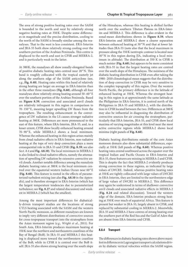
361Chapter 8: Tropical Tropopause Layer
-- Early online release --
-- Early online release --
The area of strong positive heating rates over the SASM is bounded to the north and west by relatively strong negative heating rates at 350 K. Despite some differenc-es in magnitude and the precise distribution, cooling to the north of the SASM is broadly similar among the rea-nalyses. That to the west is less consistent. ERA-Interim and JRA-55 both show relatively strong cooling over the southern portion of the Arabian Peninsula. This centre is displaced to the north and east in CFSR and MERRA-2, and is particularly weak in the latter.
At 380 K, the reanalyses all show zonally-elongated bands of positive diabatic heating rates centred near 20 ° N. This band is roughly collocated with the tropical easterly jet along the southern edge of the SASM anticyclone (see, e.g., Fig. 8.48). Heating rates within this band of relatively strong heating are larger on average in ERA-Interim than in the other three reanalyses (Fig. 8.60), although all four reanalyses show relatively strong heating around 50 - 60 ° E over the southern portion of the Arabian Peninsula. Based on Figure 8.59, convection and associated anvil clouds are relatively infrequent in this region in comparison to 70 - 150 ° E, meaning larger upwelling LW fluxes from the troposphere. The resulting enhancement in the conver-gence of LW radiation in the LS causes stronger radiative heating at 380 K. Differences are more pronounced to the east of this feature, where ERA-Interim, JRA-55, and, to a lesser extent, CFSR show locally enhanced heating around 70 - 90 ° E, while MERRA-2 shows a local minimum. Whereas the enhanced heating in this region arises mainly from cloud radiative effects in ERA-Interim, non-radiative heating at the tops of very deep convection plays a more consequential role in JRA-55 and CFSR (Fig. 8.59; see also Sect. 8.4 and Fig. A8.10). The local minimum in MERRA-2 is also linked to cloud radiative effects, namely the attenua-tion of upwelling LW radiation by extensive convective an-vil clouds. Another notable difference among the reanalysis diabatic heating rates at 380 K is the local minimum cen-tred over the equatorial western Indian Ocean near 60 ° E (Fig. 8.60). This feature is rooted in the effects of parame-terized turbulent mixing (see also Fig. A8.10 in the Appen-dix), and is therefore strongest in ERA-Interim (which has the largest temperature tendencies due to parameterized turbulence; see Fig. 8.27 and related discussion) and weak-est in MERRA-2 (which has the smallest).
Among the most important differences for diabatical-ly-driven transport studies are the locations of strong UTLS heating associated with the SASM and the western North Pacific monsoon, as different reanalyses are known to imply very different distributions of convective sources for cross-tropopause transport into the stratosphere from the Asian monsoon region (e.g., Wright et al., 2011). For South Asia, ERA-Interim produces maximum heating at 350 K near the northern and northeastern coastlines of the Bay of Bengal (BoB). In JRA-55 and MERRA-2 this heat-ing is displaced more toward the northwestern coastline of the BoB, while in CFSR it is centred over the BoB it-self. JRA-55 also shows strong heating over the south slope
of the Himalayas, whereas this heating is shifted further north over the southern Tibetan Plateau in ERA-Inter-im and MERRA-2. This difference is also evident in the zonal-mean distributions shown in Figure 8.59, where ERA-Interim and MERRA-2 show a clearer separation between enhanced heating at 30 ° N and that at lower lat-itudes than JRA-55 (note also that the local maximum in pressure along the 350 K isentropic contour is located near 30 ° N in this region during JJA, indicating a local min-imum in altitude). The distribution at 350 K in CFSR is much noisier (Fig. 8.60), but appears to be more consistent with JRA-55 in that the largest heating rates are centred over the south slope of the Himalayas. The noisiness of the diabatic heating distribution in CFSR even after taking the 1980 - 2010 climatological mean suggests that the distribu-tion of deep convection in CFSR may be very sensitive to the complex topography of this region. Over the western North Pacific, the primary difference is in the latitude of enhanced heating at 350 K. Whereas the strongest heat-ing in this region is at approximately the same latitude as the Philippines in ERA-Interim, it is centred north of the Philippines in JRA-55 and MERRA-2, with the distribu-tion in CFSR located between the two. Differences at 380 K may also be influential in diagnosing the distribution of convective sources for air crossing the stratosphere, par-ticularly that ERA-Interim, JRA-55, and CFSR show local maxima of varying magnitudes at this level near the most active convective regions while MERRA-2 shows local minima (right panels of Fig. 8.60).
Diabatic heating distributions outside of the core Asian monsoon domain also show substantial differences, espe-cially at 350 K (left panels of Fig. 8.60). Whereas positive heating rates extend southward across the equator over the tropical Indian and Pacific Oceans in ERA-Interim and JRA-55, these features are missing in MERRA-2 and CFSR. This is despite the fact that MERRA-2 evidently produces strong convection in these regions, as indicated by large values of LWCRE. Indeed, whereas positive heating rates at 350 K are tightly collocated with large values of LWCRE in ERA-Interim, they are limited to the northwestern edge of large values of LWCRE in MERRA-2. This difference may again be understood in terms of shallower convective anvil clouds and associated radiative effects in MERRA-2 (Fig. 8.24 and related discussion). Toward the western edge of the domain, ERA-Interim produces strong heat-ing at 350 K over much of equatorial Africa. This feature is present but weaker in JRA-55, largely absent in CFSR, and replaced by substantial cooling in MERRA-2. Meanwhile, JRA-55 and MERRA-2 have centres of strong heating over the southern part of the Red Sea and the Gulf of Aden that are absent from ERA-Interim and CFSR.
8.8.4 Transport
The differences in diabatic heating rates shown above mani-fest in differences in Lagrangian transport calculations driv-en by diabatic vertical velocities within the SASM region.

362
-- Early online release --
SPARC Reanalysis Intercomparison Project (S-RIP) Final Report -- Early online release --
As an extreme example, the negative heating rates below 370 K in MERRA-2 mean that diabatic transport calcula-tions are impractical unless they are initialized at the 370 K potential temperature or above (Section 8.5.2). Figure 8.61 shows the residence time for parcels traveling between the 370 K and 380 K isentropic levels within the SASM region during JJA (see Section 8.5.2 for more details). The dif-ferences can be directly linked to differences in diabatic heating rates. For example, ERA-Interim, which has the strongest heating rates in the TTL (Fig. 8.59), shows the shortest residence times (often less than 15 days). Con-versely, MERRA-2, which has the weakest heating rates within the TTL, shows the longest residence times. The minimum residence time within the SASM domain based on MERRA-2 is ~ 22 days, and many locations within the anticyclone show mean residence times greater than 25 days. Such long residence times are only found along the southeastern edge of the anticyclone in ERA-Interim. Meanwhile, CFSR and JRA-55 show relatively homoge-neous residence time distributions throughout the SASM anticyclone region, whereas MERRA-2, MERRA, and ERA-Interim show local residence time minima (indicat-ing faster uplift) in the western flank of the anticyclone.
8.8.5 Ozone
A pronounced local minimum in total column ozone dur-ing boreal summer has led researchers to dub the SASM region an ‘ozone valley’ (Bian et al., 2011; Zhou et al., 1995). Much of this regional-scale minimum in total col-umn ozone is due to low ozone mixing ratios within the UTLS anticyclone (Santee et al., 2017; Park et al., 2007). The low ozone concentrations are thought to result from extensive convective detrainment of ozone-poor tropo-spheric air and subsequent confinement within the SASM anticyclone. Ozone is parameterized and assimilated in reanalyses, as outlined and evaluated in Chapter 2 and Chapter 4 of this report.
Observational data sets
SWOOSH is an observationally-based analysis of ozone and water vapor based on a limb-sounding and solar oc-cultation instruments from the 1980s until now. For the
period we use (2005 - 2018) it is almost exactly the same as Aura MLS. The data set itself has been described by Davis et al. (2016).
Ozone
Figure 8.62 shows climatological spatial distributions of ozone volume mixing ratios at 100 hPa in the SASM region during JJA. ERA5, ERA-Interim, JRA-55, MER-RA-2, and CFSR all show relatively low ozone concentra-tions above the SASM region, although the magnitudes and spatial distributions of ozone within the anticyclone vary. Averages within the area bounded by 30 - 120 ° E and 20 - 40 ° N range from approximately 190 ppbv (JRA-55) to 325 ppbv (CFSR). All are larger than the average based on Aura MLS during 2005 - 2018 (150 ppbv), as illustrat-ed in Figure 8.62a by the SWOOSH distribution (Davis et al., 2016). For the period used here (2005 - 2018), the SWOOSH distribution for the 2005 - 2018 period shown in Figure 8.62a is almost entirely determined by Aura MLS. It is therefore important to note that Aura MLS ozone retrievals have been assimilated during recent years by ERA-Interim, ERA5, and MERRA-2 (Chapter 4; Fig 4.2). ERA5 and ERA-Interim show elongated minima in ozone mixing ratios along the southern edge of the an-ticyclone, as does SWOOSH. By contrast, JRA-55, MER-RA-2, and CFSR produce minima centred more over the Bay of Bengal, to the southeast of the anticyclone.
Figure 8.63 shows latitude–pressure cross-sections of ozone anomalies within the SASM region (30 - 120 ° E) relative to zonal-mean volume mixing ratios within the same latitude band. This view provides more infor-mation on the vertical and meridional structure of the SASM ‘ozone valley’ within the UTLS. Negative ozone anomalies correspond well to positive anomalies in ge-opotential height, with the largest anomalies typical-ly located in the upper portion of the anticyclone and slightly to the south of its centre. The ozone valley re-mains least pronounced in CFSR, for which the largest anomalies are farther south of the anticyclone centre and at a slightly lower altitude than in the other reanal-yses. However, comparison with SWOOSH again sug-gests that all five reanalyses underestimate the ampli-tude of negative anomalies associated with this feature.
Traj.MERRA2 Traj.MERRA Traj.ERAi Traj.JRA55 Traj.CFSR
residence time at 380K (days)0 60 120 180 240 300 360
Lon. (O )
-60
-30
0
30
60
Lat.
(O )
0 60 120 180 240 300 360Lon. (O )
0 60 120 180 240 300 360Lon. (O )
0 60 120 180 240 300 360Lon. (O )
0 60 120 180 240 300 360Lon. (O )
380
-60
-30
0
30
60
Lat.
(O )
420
-60
-30
0
30
60
Lat.
(O )
450
-60
-30
0
30
60
Lat.
(O )
MERRA
MERRA2
ERA-Interim
JRA55
500
NCEP-CFSR
binFrac:[ 0.000, 0.050, 0.100, 0.150, 0.300, 0.650, 0.900, 1.000,], Lon-Lat: lon[0,360],lat[-60,0,0,60],,vert[370,1800],time[2005.042,2015.958],X00: residence_time_161008_mthd_MER_day_sav1_h2oM_age_grid3D_monly_1979-2016.nc; X01: residence_time_161010_mthd_MER2_day_sav1_h2oM_age_grid3D_monly_1980-2016.nc; X02: residence_time_161014_mthd_ERAi_day_sav1_h2oM_age_grid3D_monly_1979-2016.nc; X03: residence_time_161012_mthd_JRA55_day_sav1_h2oM_age_grid3D_monly_1979-2016.nc; X04: residence_time_161016_mthd_CFSR_day_sav1_h2oM_age_grid3D_monly_1979-2010.nc;
12 18 20 22 24 26 30 36 180
residence time (days)
Residence Time @ 380-K (2005-2015 JJA)Asian monsoon
Figure 8.61: Residence time (days) between 370 K and 380 K, displayed at 380 K, during JJA 2005 - 2015 (for details see Fig. 8.31; Section 8.5.2).

363Chapter 8: Tropical Tropopause Layer
-- Early online release --
-- Early online release --
ERA5, ERA-Interim and JRA-55 show substantial nega-tive ozone anomalies (- 10 % or larger) extending down-ward to 250 or even 300 hPa within the SASM region, whereas anomalies are more confined to the lower TTL (p ≤ 200 hPa) in MERRA-2. None of the reanalyses re-produce observed positive anomalies relative to the zon-al mean at lower altitudes, which are located both below and to the south of the anticyclone core according to the SWOOSH distribution. These positive anomalies may be related to anthropogenic emissions of ozone precursor
species and subsequent convective transport. As these emissions are not represented in the simple ozone schemes used in the forecast models (Chapter 2; Table 2.10), such effects could only enter the reanalysis products through the data assimilation. Although temporal variations in SASM ozone are not evaluated here, users should be aware that changes in assimilated ozone data over time (Chapter 4; Figs. 4.1 and 4.2), especially vertically-resolved profile data (Fig. 4-2), may lead to discontinuities in reanalysis representations of the SASM ozone valley.
Figure 8.62: Spatial distributions of JJA-mean ozone mixing ratio [ppbv] on the 100 hPa isobaric surface based on (a) SWOOSH (Davis et al., 2016), (b) ERA5, (c) ERA-Interim, (d) JRA-55, (e) MERRA-2, and (f) CFSR. Reanalysis ozone products are averaged over 1980 - 2010; SWOOSH data are averaged over 2005 - 2018. The 16700 m contour in 100-hPa geopotential height based on the cor-responding data sets is shown as a white dashed line in each panel for context. Geopotential height in panel (a) is from ERA-Interim.
Figure 8.63: Latitude–pressure distributions of normalized anomalies [%] in JJA-mean ozone mixing ratios within 30 - 120 ° E relative to zonal-mean values for the corresponding zonal bands derived using (a) SWOOSH, (b) ERA5, (c) ERA-Interim, (d) JRA-55, (e) MERRA-2, and (f) CFSR. Reanalysis ozone products are averaged over 1980 - 2010; SWOOSH data are averaged over 2005 - 2018. Absolute geopotential height anomalies in the 30 - 120 ° E band relative to the zonal mean are shown as white dashed contours at values of 100 and 125 m. Geopotential height anomalies relative to the zonal mean in panel (a) are from ERA-Interim.

364
-- Early online release --
SPARC Reanalysis Intercomparison Project (S-RIP) Final Report -- Early online release --
8.8.6 Regional analysis of clouds and radiative effects
In this Section, we focus on a regional analysis of cloud and radiative properties in the SASM, which is recognized as the location of the largest discrepancies among reanalyses and climate models (Tissier and Legras, 2016; Johansson et al., 2015; Heath et al., 2014).
We compare the five reanalyses CSFR, JRA-55, MERRA-2, ERA-Interim and ERA-5 and use satellite products as refer-ences. The comparison includes the ERA5 reanalysis of EC-MWF (Hersbach et al., 2020), which is a new reanalysis based on a new generation of the ECMWF Integrated Forecasting System (IFS) model (cycle CY41R2) with a gap of more than 10 years with respect to the previous ERA-Interim reanalysis.
Observational data sets
For comparison the reanalyses are compared with differ-ent satellite products which contain strong assumptions.
We use the 2B-FLXHR-LIDAR radiative heating product version 4 (FLXHR) that combines cloud data from the A-train satellite instruments CLOUDSAT, CALIPSO and MODIS to calculate radiative heating (L’Ecuyer et al., 2015; Henderson et al., 2013) 1. This product depends on a number of other products, retrieval algorithms and assumptions, and temperature profiles from the ECMWF AUX product; it is therefore liable to biases and errors. Besides this, the A-train satellites are helio-synchronous and therefore the daytime and nighttime observations occur at fixed hours (close to 1:30 and 13:30 in local time) and do not sample properly the daily cycle of convection, especially over land where convection has its maximum in late afternoon. Nev-ertheless, FLXHR is based on comprehensive observations rather than modelled properties of clouds and represents a state-of-the-art estimate of the radiative effect.
The 2B-CWC-RVOD retrieves ice water path from the CLOUDSAT radar reflectivity and the visible optical depth
from MODIS. The 2C-ICE product retrieves the ice water path from the radar reflectivity and the backscatter coeffi-cient of the CALIOP lidar. They both use Rodgers optimal estimation in the retrieval. Total condensates are available from the 2B-CWC-RVOD product version 4 (Austin et al., 2009), which is used in FLXHR version 4, and the ice profile from the 2C-ICE product version 4 (Deng et al., 2013, 2015).
Clouds and radiative effects
The cloud properties differ quite significantly among the reanalyses and the radiative properties vary accordingly. Figure 8.64 shows that the maximum cloud cover in the ERA5 is smaller than in the ERA-Interim in the monsoon region, especially in the maritime regions that surround Asia. The altitude of the maximum cloud cover, not shown, is also lower by about 3 K on the average in potential tem-perature. As a result of these changes in the high clouds, the cloud radiative effect is also strongly modified. Fig-ure 8.65 illustrates the cloud radiative properties in the SASM longitude range (73 - 97 ° E) for the five reanalyses investigated in this Section. The two ECMWF reanaly-sis differ by the fact that the ERA5 cloud is smaller and located at a lower altitude than in the ERA-Interim, es-pecially over the oceans (see cloud cover Section below). Therefore, the maximum of the cloud radiative effect is shifted downward by about 2 km, and the mean zero level of net radiative heating is left rather unperturbed by the clouds except over 20 - 40 ° N where continental convection dominates and it will be seen below that this is mostly an effect of the Tibetan plateau. Two other reanalyses, CFSR and JRA-55, display cloud radiative heating patterns that are in fairly good agreement with ERA5 but with much reduced amplitude for JRA-55. MERRA-2 exhibits a very different pattern from other reanalysis with a strong ra-diative heating in the 0 - 20 ° N latitude range and from 6 km to 12 km and a strong cooling above from 12 km to 16 km. As a consequence, an island of positive all sky radiative heating is observed between 8 km and 10 km and the zero level of radiative heating is shifted upward by one kilometer by the clouds between 10 ° S and 30 ° N.
1 T2B-FLXHR-LIDAR and all the CLOUDAT/CALIPSO products mentioned in this study (2B-GEOPROF, 2B-CWC-RVOD, 2C-ICE) are available at http://www.cloudsat.cira.colostate.edu/data-products
Figure 8.64: Cloud cover in [fraction] at the level of the maximum cloud in the SASM domain for ERA-Interim (left) and ERA5 (right), July - August 2005 - 2010.

365Chapter 8: Tropical Tropopause Layer
-- Early online release --
-- Early online release --
This is contrary to the ERA-Interim case where it is shift-ed downward by about 2 kilometers over the same latitude range. In the following, we investigate more details about these discrepancies and their causes.
In order to separate land from ocean and, among land, the high orography of the Tibetan plateau from the rest of Asia, we divide the SASM domain into a set of regions as indicated in Figure 8.66. We focus on six regions that en-compass most of the convective activity during SASM and its variability: Bay of Bengal (BoB), Indian Subcontinent (Indian Sub), South China, Sea of China and Philippine Sea (SCSPhi), Indochinese Peninsula (Pen) and the Tibet-an-Plateau.
From the heating archive of the five reanalyses, the cloud heating has been obtained by removing the clear-sky contribution from the all-sky value. As the clear-sky heating rates are not available for JRA-55 and CFSR, we use ERA5 as a reference. It has been checked with ERA5, ERA-Interim and MERRA-2 that the discrep-ancies among clear sky radiative heating rates are at least one order of magnitude smaller than the all sky discrepancies, except near the ground over land where
differences in albedo induce also differences in short-wave heating. The total shortwave heating rate is cal-culated using the clear sky sun variation as integrator.
Figure 8.65: Cloud radiative heating as dθ /dt [K/day] for ERA-Interim, ERA5, CFSR, JRA-55 and MERRA-2 aver-aged over the 73 - 97 ° E longitude range during July - Au-gust 2005 - 2010. Black line: zero level of cloud radiative heating. Dashed yellow contour: zero level of clear sky total radiative heating. Green contour: zero level of all sky total radiative heating. White contour levels: poten-tial temperature [K], intervals of 10 K. Red crosses: cold point tropopause. The vertical scale is the barometric altitude based on the standard atmosphere.
BoB
Indian Sub
SCSPhi
South China
Pen
Tibetan Plateau
70 80 90 100 110 120 130
6
12
18
24
30
36
42
Region mask
Figure 8.66: Longitude-latitude distribution of considered SASM regions including two maritime regions: Bay of Bengal (BoB) and Sea of China and Philippine Sea (SCSPhi); and four con-tinental regions: Indian Subcontinent (Indian Sub), South China, Indochina Peninsula (Pen) and the Tibetan Plateau. The Tibetan Plateau is defined as the region of altitude higher than 3800 m. Other regions seen in this map are not used in this study.

366
-- Early online release --
SPARC Reanalysis Intercomparison Project (S-RIP) Final Report -- Early online release --
The comparison is based on July and August months of the 2007-2010 period, for which the FLXHR product is availa-ble for both night-time and day-time orbits.
Figure 8.67 shows that JRA-55 differs from the other rea-nalyses in producing very small cloud shortwave heating. Over maritime regions (BoB and SCSPhi), the reanaly-ses have maximum radiative heating near 350 K with fast decay above, while FLXHR displays a maximum higher up at ~ 358 K and larger values than all reanalyses in the 360 - 390 K range. MERRA-2 is the reanalysis with the low-est and narrowest maximum. The discrepancy from FLXHR is the largest over the maritime regions, where FLXHR sam-ples convection near its mid-day maximum. Our calcula-tion might therefore generate a posi-tive bias with a large maximum at the altitude of maximum cloud cover (see also Fig. 8.69, below). The discrepancy is strongly reduced over China and In-dia with respect to ECMWF reanalysis and CFSR while MERRA-2 retains its characters. For FLXHR and all reanal-yses, the radiative heating maxima are shifted upward over land with respect to ocean. The Indochinese Peninsula (Pen) region presents intermediate pat-terns between land and ocean. Over the Tibetan Plateau, a diversity of patterns is obtained and the sole reanalysis that displays the neat double peak structure of FLXHR is ERA5, the lower peak being due to low level clouds (as 330 K is close to the surface in this region). Notice, however, that the typically late
afternoon convection of the Tibet-an Plateau is not well sampled by the A-train satellites. It is noticeable that, except over this region, the CFSR and ERA5 curves are very close, closer than ERA5 and ERA-Interim.
Figure 8.68 shows the cloud long-wave heating. In the maritime re-gions, CFSR and ERA5 are still very close and follow closely the FLXHR curve with small cooling above 350 K and warming below. JRA-55 and ERA-Interim form another group with warming all the way down from 370 K. MERRA-2 exhibits a very strong cooling-warming pattern, typical of the effect of fat convective anvils, with a crossover at 350 K. Over Indian Sub and South China, the agreement persists between CFSR and ERA5 on one side and between ERA-Interim and JRA-55 on the oth-er side but now FLXHR agrees bet-ter with the second pair above 370 K where it produces heating instead of
cooling. MERRA-2 displays the same pattern than over the ocean but attenuated. As for shortwave heating, In-dochinese Peninsula (Pen) shows intermediate patterns.
Over the Tibetan Plateau, CFSR agrees with ERA-Inter-im but not with ERA5. No reanalysis agrees well with FLXHR and the MERRA-2 curve shows multiple cross-ings with the zero line. The fact that reanalyses disagree even on the sign of the cloud longwave radiative effect above 350 K is not totally surprising as the antagonist warming effect of cirrus and cooling effect of the under-lying thick anvils largely balance in this region (Johans-son et al., 2015).
Figure 8.67: Cloud short-wave radiative heating as dθ/dt [K/day] for ERA5, ERA-Interim, JRA-55, CFSR and MERRA-2 as potential temperature tendencies for the six regions shown in Fig. 8.66: BoB, Indian Sub, South China, SCSPhi, Pen and Tibetan Plateau as a function of altitude in potential temperature. The aver-age is performed over July - August of 2007 - 2010. Black curve shows the FLXHR satellite profile, and other colors the reanalyses as indicated in legend.
Figure 8.68: Same as Fig. 8.67 but for cloud long-wave heating [K/day].

367Chapter 8: Tropical Tropopause Layer
-- Early online release --
-- Early online release --
In order to explore the origin of such discrepancies, Figure 8.69 shows the cloud cover profiles for the reanalyses and for the 2B-GEOPROF-LIDAR product used in FLXHR (Mace and Zhang, 2014). Such comparison must be consid-ered carefully as the notion of cloud cover is not necessarily defined in the same way between observations and models. Nevertheless, we do not see here any pattern that would ex-plain MERRA-2 differences with the other reanalyses. The reanalyses and 2B-GEOPROF-LIDAR cloud cover are in good agreement over South China and Indian Sub, but for the tendency of JRA-55 to maintain significant cloud cover at very high altitude. The dispersion is larger over the maritime regions and not surprisingly over the Tibetan Plateau where, however, all reanalyses except MERRA-2 show a double maximum structure with a layer of low clouds. In all cases, the higher cloud cover over continental regions is consistent with the cloud radiative profiles.
The water condensate profiles of the re-analyses and two A-train satellite prod-ucts (2B-CWC-RVOD and 2C-ICE) are shown in Figure 8.70. An evaluation of 2C-ICE against other satellite products and ground observations can be found in Deng et al. (2013, and 2015). These curves display the non-precipitating component which is usually the one used for radiative calculations. Again, ERA5 and CFSR are very close over the maritime region but CFSR exceeds ERA5 by about 70 % above 340 K over the land. There is a very small amount of condensates in JRA-55 which drops rapidly to zero at high levels. Therefore, the large cloud cover found in Figure 8.69 is of no consequence and this ex-plains the overall low cloud radiative ef-fect of JRA-55. On the contrary, MER-RA-2 exhibits a large maximum in the
condensates between 340 K and 350 K over the maritime region, due to thick anvils mainly consisting of ice, which is clearly correlated with the warming layer in the longwave heating and to the sharp maximum in the shortwave heat-ing. The strong longwave cooling above is due to the small emission of this thick opaque ice layer. The same pattern is seen over land but weaker and at high-er altitude, again in good correlation with the radiative heating. The level of zero crossing in the longwave heating is also located just at the top of the con-densate layer in CFSR and ERA5. The smaller amount of condensates in the anvil layers of ERA-Interim and JRA-55 is a good candidate to explain why heating by cirrus clouds overwhelms the cooling effect of anvils above 350 K.
It is quite certain that these water condensates profiles are the main explanation of the discrepancies visible in the ra-diative heating above the SASM region and that the compe-tition between the signatures of the convective cloud anvils and the cirrus clouds is the key factor as already shown by Johansson et al. (2015).
The satellite products can hardly be compared to the non-precipitating water condensates in models since they measured both non-precipitating and precipitating conden-sates together; separating the two requires ad hoc filtering and corrections. As the ERA5 archived data includes also the rain and snow variables we also compare in Figure 8.70 the total condensate profile of ERA5 with two A-train satel-lite products. The agreement between the three curves is best over the continental regions (outside the Tibetan Plateau).
Figure 8.69: Same as Fig. 8.67 but for cloud cover [fraction].
Figure 8.70: Non-precipitating cloud condensates (ice and water; in [mg/kg]) for the four reanalyses; plain solid curves. Additional, total cloud condensates are shown for ERA5, including snow and rain (light blue dotted curve), and for the 2B-CWC-RVOD (black dotted curve) and 2C-ICE (magenta dotted curve) A-train satel-lite products; (all in [mg/kg]). Otherwise same period and regions as for Fig. 8.67.

368
-- Early online release --
SPARC Reanalysis Intercomparison Project (S-RIP) Final Report -- Early online release --
The whole profiles of ERA5 and 2B-CWC-RVOD are very close over Indian Sub and South China while 2C-ICE is larger below the top of the convective cloud anvils. Over the maritime regions, ERA5 has less condensates than the satellites products and the separation increases below 350 K where 2C-ICE pro-vides also much larger values than 2B-CWC-RVOD.
Over the Tibetan-Plateau, ERA5 displays a large deficit of condensates with respect to the satellite products around 340 K. Only the ERA-Interim and JRA-55 show a profile with a strong maximum in this region in agreement with the cloud cover but with a much too weak value. Even if the A-train satellite products are likely to contain some biases over the Tibetan-Plateau, the discrepancies with respect to analyses in this region might be for a large part due to a general under-representation of the low-level convection (Li et al., 2016, 2017).
Finally, Figure 8.71 shows the daily cycle of the cloud radiative heating for three regions – maritime (BoB),
continental (Indian Sub) and the Tibetan-Plateau and four reanalyses (excluding CFSR). The contrast is strong between JRA-55 which shows a very weak daily cycle and MERRA-2 which shows a very strong cycle with intense nocturnal cooling between 345 K and 365 K (~11 km and 15 km) due to persistent thick convective cloud anvils. In the BoB region, the diurnal maximum of MERRA-2 is located at the lowest level at 345 K (~ 11 km) while the ERA-Interim is at the highest level at 355 K (~ 13.5 km). Over India, the diurnal radiative heating in MERRA-2 is attenuated and slightly shifted towards afternoon with re-spect to BoB. There is no attenuation respective to mari-time value but a noticeable afternoon shift in ERA-Interim and ERA5. In addition, the vertical location of the maxi-mum rises by about 10 K in both reanalyses but remains lower in ERA5. Over the Tibetan-Plateau, where other reanalyses show weak radiative heating ERA5 exhibits a strong maximum that reaches 380 K (~ 17 km), which is as-sociated with high penetrative convection in this region, a distinguished signature of ERA5.
Figure 8.71: Daily cycle of cloud radiative heating as d /dt [K/day] calculated over July - August 2005 - 2010 for ERA-Inter-im, MERRA-2, JRA-55 and ERA5 (columns) and for the three regions BoB, Indian Sub and Tibetan-Plateau (rows). The figure is based on hourly data for ERA5, 3-hourly data for MERRA-2 and ERA-Interim, and 6-hourly date for JRA-55.

369Chapter 8: Tropical Tropopause Layer
-- Early online release --
-- Early online release --
8.8.7 Key findings and recommendations
Key findings
� Modern reanalyses agree well regarding the clima-tological position and extent of the SASM anticy-clone, although there are notable differences in the distribution of SASM anticyclone centre locations among different reanalyses. Distinct bimodality of the SASM anticyclone centre location based on dai-ly data is only present in NCEP-NCAR R1. (Section 8.8.1)
� Reanalyses indicate slightly higher CPT temper-atures and lower CPT heights in the SASM anticy-clone compared to GNSS-RO satellite observations. (Section 8.8.1)
� Climatologies of SASM anticyclone moments (cen-troid location, aspect ratio, angle, excess kurtosis) computed using MSF on isentropic surfaces to de-fine the SASM anticyclone edge show good agree-ment among the MERRA, MERRA-2, ERA-Interim, JRA-55, and CFSR/CFSv2 reanalyses. Good qualita-tive agreement is seen in the evolution of SASM an-ticyclone area defined using MSF, but MERRA and MERRA-2 show larger areas and consequently longer monsoon seasons, along with more significant ap-parent increasing trends in SASM anticyclone area. (Section 8.8.1)
� Omega fields from ERA-Interim, JRA-55, MERRA-2, and CFSR reanalyses agree well on the overall spatial pattern within the SASM domain. However, regional discrepancies exist, especially over locations of fre-quent convection such as the western coast of India and the Bay of Bengal. (Section 8.8.2)
� Diabatic heating distributions within the SASM re-gion differ significantly among reanalyses, especially with respect to the mean latitudinal location of the maximum heating rates connecting the convective detrainment layer to the lower stratosphere. This maximum is located progressively further north in ERA-Interim, JRA-55, and CFSR, and is missing entirely from MERRA-2. These differences can be attributed to differences in the dominant diabatic processes in the UT above the SASM region: cloud-in-duced radiative heating in ERA-Interim, convective heating in JRA-55 and CFSR, and cloud-induced ra-diative cooling in MERRA-2. (Section 8.8.3)
� The depth and location of convection within the SASM and surrounding regions varies among the re-analyses. These differences impact implied convec-tive transport over the Bay of Bengal, the Himalayan South Slope, the south-eastern Tibetan Plateau, and
the western North Pacific, as well as over East Asia and equatorial Africa. Differences in the distribution and magnitude of diabatic heating near the tropo-pause (380 K) are likewise strongly affected by dif-ferences in the distribution of convection and related clouds. (Section 8.8.3)
� Residence times based on diabatic Lagrangian trans-port calculations are shortest in the centre of the SASM anticyclone for all reanalyses. The absolute magnitudes of residence time in the SASM anticyclone show large differences, varying from a minimum of 14 days (ERA-Interim) to a maximum of 22 days (MER-RA-2) during the JJA season. (Section 8.8.4)
� Despite differences in magnitude and in the loca-tions of local extrema, distributions of ozone volume mixing ratios within the SASM anticyclone are qual-itatively consistent among reanalyses and broadly consistent with observations. However, none of the evaluated reanalyses are able to fully reproduce the low ozone mixing ratios within the SASM ‘ozone val-ley’. (Section 8.8.5)
� Cloud properties differ greatly among reanalyses as these properties are weakly constrained by assimilat-ed observations. The radiative effect of clouds is used here as a metric in the SASM domain. In all reanal-yses, maximum cloud cover is found between 350 K and 355 K over maritime regions and near 360 K over land. The maximum shortwave cloud heating rates essentially follow the maximum cloud cover. The longwave cloud heating rate combines the effect of thick anvils (warming below and cooling above) and the warming effect of overlying cirrus. The balance above clouds can be either positive or negative de-pending on the reanalysis. (Section 8.8.6)
� MERRA-2 displays a very strong anvil signature in contrast to all other reanalyses and satellite products. The discrepancies in the long-wave cloud heating rates are mostly explained by the ice content of high clouds in the reanalyses. Overall, the heating rates based on ERA5 are closest to the FLXHR satellite product. ERA5 is distinguished by lower cloud maxima on the average but stronger penetrative convection, in par-ticular over the Tibetan Plateau. (Section 8.8.6)
Key recommendations
� For subsequent analyses involving the position of the SASM anticyclone centre it is recommended to use more recent reanalyses. In particular, researchers are encouraged to avoid NCEP-NCAR R1 and NCEP-DOE R2 when possible, proceed with caution if it is neces-sary to use one of these two reanalyses, and assess the sensitivity of results to the choice of reanalysis regard-less of which reanalysis is used. (Section 8.8.1)

370
-- Early online release --
SPARC Reanalysis Intercomparison Project (S-RIP) Final Report -- Early online release --
� The geopotential height field from the MERRA-2-ANA pressure-level data set features spurious enhancements over the steep orography of the Himalaya Mountains due to a conversion error. For analyses that are sensitive to this issue, any use of MERRA-2-ANA data should rely on the model-level products only. MERRA-2-ASM products are unaffected by this issue. (Section 8.8.1)
� Transport simulations for the SASM domain that use dia-batic heating rates to represent vertical motion should use multiple reanalyses if possible and carefully consider the representation of convective sources to the TTL. MERRA-2 diabatic heating rates should only be used at 370 K potential temperature level and above. (Sections 8.8.3 and 8.8.4)
� Reanalyses capture the existence of the ozone mini-mum in the UTLS above the SASM but do not reliably reproduce its observed distribution or magnitude. Use of reanalysis ozone products in this region is appro-priate for evaluation of internal reanalysis behaviour. Other applications should keep in mind the relatively simple formulation of the ozone models (see Chapters 2 and 4) and include careful validation against observa-tions. (Section 8.8.5)
� Cloud and radiative heating for SASM regions should be used with caution for all reanalyses. However, ERA5 is most consistent with the satellite-based FLXHR product. (Section 8.8.6)
8.9 Summary, Key Findings, and Recommendations
Chapter 8 investigates the extent to which reanalysis data sets are able to reproduce key characteristics of the TTL. Representa-tions of the cold point and lapse rate tropopause are evaluated based on comparison of tropopause zonal mean profiles and time series to observational records from radio occultation and radiosonde data. The vertical structure of the TTL is then assessed by comparing reanalysis temperature profiles at model-level resolution to high-resolution GNSS-RO temperature profiles.
Basic dynamical processes and circulation patterns are evaluated by comparing zonal-mean and tropical-mean distri-butions of diabatic heating, as well as by means of Lagrangian trajectory simulations of transport within the TTL. Final dehydration locations and temperatures as well as TTL residence times derived from these trajectory simulations are com-pared among the reanalyses and validated against vertical velocity estimates derived from satellite observations of water vapor. Large-scale wave forcing is analysed based on the characteristic horseshoe-shaped structure that results from the superposition of Rossby and Kelvin responses to intense convective heating. Comparison against NOAA outgoing long-wave radiation allows an assessment of spatiotemporal variability in this wave response. A zonal wavenumber-frequency spectral analysis is also carried out to describe and evaluate equatorial wave activity in the reanalyses. Long-term changes in the width of the tropical belt are derived based on the tropical jet and tropopause break positions, two metrics which are known to correlate only weakly with Hadley cell extent. Tropical-width metrics calculated based on instantaneous longi-tudinally-resolved and zonal-mean annual-mean fields are compared with each other. Owing to the lack of observational data for validating the tropical width diagnostics, the extent to which changes may be considered robust is determined based on statistical methods and consistency among the reanalyses. Finally, analysis of the upper troposphere and lower stratosphere above the South Asian Summer Monsoon (SASM) highlights some key differences in reanalysis performance within the TTL via focus on regional and seasonal aspects of the SASM anticyclone.
Key findings
� Advances in reanalysis and observational systems over recent years have led to a clear improvement in TTL reanalysis products over time. In particular, the reanalyses ERA-Interim, ERA5, MERRA2, CFSR, and JRA-55 show very good agreement after 2002 in terms of the vertical TTL temperature profile, meridional tropopause structure, and inter-annual variability. Long-term temperature trends from reanalyses and adjusted radiosonde data indicate significant cooling in the upper TTL during 1979 - 2005 (above the cold point). (Section 8.2)
� While climatological TTL temperatures from reanalyses agree very well with observations with relatively small low biases, the cold point and lapse rate tropopause show warm biases, most likely related to the fact that the discrete values corresponding to reanalysis model levels are unable to reproduce the observed minimum temperature as recorded in a near-continuous profile. (Section 8.2.2)
� Cloud fields in the tropical UTLS vary greatly in both magnitude and vertical distribution across reanalyses. Differenc-es in cloud fraction and cloud water content impact the radiation budget both at the top-of-atmosphere and within the UTLS, and the effects of differences in cloud and convection parameterizations can be identified in vertical profiles of temperature and humidity in the tropical troposphere. (Section 8.3)

371Chapter 8: Tropical Tropopause Layer
-- Early online release --
-- Early online release --
� There are large differences among reanalysis diabatic heating products within the TTL, which are known to influ-ence transport statistics and rates of ascent in trajectory simulations of cross-tropopause transport in this region. Differences among reanalysis diabatic heating rates in the tropical UTLS are not limited to any one component: longwave, shortwave, and non-radiative components all show substantial discrepancies. (Section 8.4)
� Lagrangian transport studies demonstrate large differences in reanalysis temperatures at the dehydration point and in TTL residence times. However, the data sets agree on the spatial distribution of dehydration locations and pro-duce roughly similar distributions, seasonal cycles, and interannual variations of TTL residence time. (Section 8.5)
� Equatorial wave activity and corresponding temperature anomaly patterns at 100 hPa are similar among the reanal-yses, including the characteristic horseshoe-shaped structures that resemble the stationary wave response to tropical heating. However, the strength of the wave activities, their spectral magnitudes, and the intensity of temperature response differ among the reanalyses, with the latter differences depending on the aspects of the dynamical model and/or assimilation system. (Section 8.6)
� Metrics of the width of the TTL based on the zonally-resolved subtropical jet and tropopause break show robust changes in only a few regions and seasons and poor agreement of the resulting zonal-mean annual-mean values. The diagnostics based on the zonal-mean subtropical jet and tropopause break, on the other hand, suggest stronger trends in the width of the TTL than their zonally-resolved counterparts. Overall, the two subtropical jet diagnostics are more consistent than the two tropopause break diagnostics, possibly related to smoother variations in the zonal wind field relative to the tropopause break. (Section 8.7)
� Modern reanalyses agree well regarding the climatological position and evolution of area extent and moments of the SASM anticyclone, although there are notable differences in the distribution of SASM anticyclone centre locations. All of the reanalyses indicate slightly higher CPT temperatures and lower CPT heights in the SASM anticyclone compared to GNSS-RO satellite observations. (Section 8.8.1)
� Distributions of ozone volume mixing ratios within the SASM anticyclone are qualitatively consistent among rea-nalyses and broadly consistent with observations. However, none of the evaluated reanalyses are able to reproduce the low ozone mixing ratios within the SASM anticyclone. (Section 8.8.5)
� Cloud properties, convection, radiative heating, and omega fields for the SASM UTLS differ significantly among reanalyses on a regional scale as these properties are only weakly constrained by assimilated observations. These differences impact derived transport processes in the UTLS, and residence times based on diabatic Lagrangian transport calculations reveal large differences. (Sections 8.8.2, 8.8.3, 8.8.4, 8.8.6)
Key recommendations
� In the TTL, temperature on native model levels should be used rather than the standard pressure-surface data sets. Various diagnostics such as the cold point and lapse rate tropopause and the analysis of equatorial waves are demon-strably improved when model-level data are used. For a more realistic representation of the tropical tropopause lev-els, data sets that combine low temperature biases with high vertical resolution should be used. (Sections 8.2 and 8.6)
� Long-term drifts in high cloud fraction, OLR, and LWCRE are present in almost all reanalyses, and often disagree in terms of sign, timing, or magnitude. These products should generally not be used for trend or time series analysis with-out independent verification. Among the reanalyses, ERA5 shows greater stability in time and stronger correlations with observed variability for these cloud and radiation metrics and may therefore offer a more reliable characterization of long-term variations in related metrics relative to earlier reanalyses. (Section 8.3)
� Given large differences in reanalysis diabatic heating products and related metrics within the tropical UTLS, re-searchers using these fields to drive or nudge model simulations of this region should use multiple reanalyses when-ever possible. (Sections 8.4 and 8.5)
� When applying metrics of tropical width based on the subtropical jet or tropopause break, it is recommended to use multiple reanalyses and to be aware of the caveat that the zonal-mean diagnostics suggest stronger trends than their zonally-resolved counterparts. (Section 8.7)

372
-- Early online release --
SPARC Reanalysis Intercomparison Project (S-RIP) Final Report -- Early online release --
� For analyses involving the SASM anticyclone it is recommended to use more recent reanalyses. In particular, research-ers are encouraged to avoid NCEP-NCAR R1 and NCEP-DOE R2 data sets and the geopotential height field of the MERRA-2-ANA pressure-level data when possible. (Section 8.8.1)
� Transport simulations for the SASM domain that use diabatic heating rates to represent vertical motion should use multiple reanalyses if possible and carefully consider the representation of convective sources to the TTL. MERRA-2 diabatic heating rates should only be used at 370 K potential temperature level and above. (Sections 8.8.3, 8.8.4)
� Ozone in the UTLS above the SASM should be carefully validated against observations, and cloud and radiative heat-ing should be used with caution for all reanalyses. (Sections 8.8.5, 8.8.6)
Figure 8.72: Diagnostic evaluation for Chapter 8 on the Tropical Tropopause Layer (TTL). Top: Climatological and dynami-cal TTL characteristics (Sections 8.2-8.7) and bottom: South Asian Summer Monsoon (SASM) characteristics (Section 8.8). CPT: Cold Point Tropopause, LRT: Lapse Rate Tropopause, HCC: High Cloud Cover, CWC: Cloud Water Content, OLR: Outgoing Longwave Radiation, LW: Long Wave, ZM: Zonal Mean, UT: Upper Troposphere, LS: Lower Stratosphere, LZRH: Level of Zero Radiative Heating, CP: Cold Point.

373Chapter 8: Tropical Tropopause Layer
-- Early online release --
-- Early online release --
Acknowledgements
We acknowledge the institutions involved in the production and dissemination of the reanalysis data NCAR is support-ed by grants from the National Science Foundation.
(8.3, 8.4, 8.8.3, 8.8.5) Contributions by JSW to these Sections were supported by funding from the National Natural Sci-ence Foundation of China (grant number 41761134097).
(8.3) We thank Xianglei Huang for advice on interpreting satellite observations of outgoing LW radiation, Peter Bechtold, Andrea Molod, and Guang J. Zhang for clarify-ing aspects of the cloud, convection, and turbulence pa-rameterizations in the reanalysis forecast models, Xiaoyi Sun for conducting the initial data processing for high cloud fields and OLR, and Yi Huang for recommenda-tions on methodology and presentation.
(8.4) We thank Stephan Fueglistaler for providing the tur-bulent mixing temperature tendency for ERA-Interim, SHADOZ data, ERA-Interim ozone climatology, and many helpful suggestions.
(8.8.1) The research leading to these results has received funding from the European Communities Seventh Framework Programme (FP7/2007 - 2013) under grant agreement No. 603557.
(8.8.5) We thank Xiaolu Yan for providing context on the Asian monsoon ozone valley and its origins.
(8.8.6) BL acknowledges support from the TTL-Xing ANR-17-CE01-0015 project of Agence Nationale de la Recherche.
Figures 8.2, 8.3, 8,4, 8.5, 8.6, 8.7, 8.8, and 8.9 are adapted from Tegtmeier et al. (2020). Figures 8.10, 8.11, 8.12, 8.13, 8.14, 8.15, 8.17, 8.24, and 8.25 are adapted or reproduced from Wright et al. (2020). Figures 8.20, 8.21, and 8.26 are updated from Wright and Fueglistaler (2013). Fig. 8.38 is modified after Kim et al. (2019). Figure 8.47 is modi-fied from Nützel et al. (2016). All these reproductions are made under a creative commons attribution 3.0 or 4.0 li-cense (https://creativecommons.org/licenses/by/3.0/ or https://creativecommons.org/licenses/by/4.0/, respectively).
Data availability
(8.8.1) For some of the analyses, NCEP-DOE R2, CFSR, JRA-25 and JRA-55 data were provided by the Research Data Ar-chive (RDA) of the Computational and Information Systems Laboratory at the National Center for Atmospheric Research via https://rda.ucar.edu/. NCAR is supported by grants from the National Science Foundation. NCEP-NCAR R1, ERA-In-terim and MERRA/MERRA-2 data were obtained from NOAA/OAR/ESRL PSD at https://www.esrl.noaa.gov/psd/, from ECMWF at https://apps.ecmwf.int/datasets/data/interim-full-daily/levtype=pl/ and from GES DISC at https://disc.gsfc.nasa.gov/ (partly via mirador.gsfc.nasa.gov), respectively. ERA5 diagnostics have been produced using data extracted from Copernicus Climate Change Service. A-train data have been obtained and processed at ICARE/AERIS Data Centre.
(8.8.6) The satellite data are provided by the AERIS/ICARE data center http://www.icare.univ-lille1.fr. ERA5 data were generated using Copernicus Climate Change Service Information.
Author contributions
ST and KK wrote Chapter 8 with contributions from all coauthors. The data, figures and text for the individual sections were compiled by the following coauthors listed by sections.
Section 8.1: ST, KKSection 8.2: ST, SD, II, BL, RPK, JSWang, TWSection 8.3: JSWright (JSW)Section 8.4: JSWSection 8.5: 8.5.1: TW; 8.5.2: TW; 8.5.3: JSW, TBSection 8.6: 8.6.1: EN, MF; 8.6.2: YHK, MFSection 8.7: NAD, SD; 8.7.1: GLM; 8.7.2: CRH, 8.7.3: TB, NAD, GLM, CRHSection 8.8: 8.8.1 MN, GLM, ST, KK; 8.8.2: CRH, KK; 8.8.3: JSW, KK; 8.8.4: TW, KK; 8.8.5: JSW; 8.8.6: BLSection 8.9: All authors

374
-- Early online release --
SPARC Reanalysis Intercomparison Project (S-RIP) Final Report -- Early online release --
References
Abalos, M., B. Legras, F. Ploeger, and W.J. Randel, 2015: Evaluating the advective Brewer-Dobson circulation in three reanalyses for the period 1979–2012. J. Geophys. Res., 120, 7534 - 7554, ooi: 10.1002/2015JD023182.
Adam, O., et al., 2018: The TropD software package (v1): standardized methods for calculating tropical-width diagnostics. Geosci. Model Dev., 11, 4339 - 4357, doi: 10.5194/gmd-11-4339-2018.
Anthes, R.A., et al., 2008: The COSMIC/FORMOSAT-3 Mission: Early Results. B. Am. Meteor. Soc., 89, 313 - 333, doi: 10.1175/BAMS-89-3-313,.
Austin, R.T., A.J. Heymsfield, and G.L. Stephens, 2009: Retrieval of ice cloud microphysical parameters using the CloudSat millimeter-wave radar and temperature. J. Geophys. Res., 114, doi: 10.1029/2008JD010049.
Bechtold, P., et al., 2008: Advances in simulating atmospheric variability with the ECMWF model: From synoptic to decadal time-scales. Q. J. R. Meteor. Soc., 134, 1337 - 1351, doi: 10.1002/qj.289.
Bechtold, P., et al., 2014: Representing equilibrium and nonequilibrium convection in large-scale models. J. Atmos. Sci., 71, 734 - 753, doi: 10.1175/JAS-D-13-0163.1.
Bergman, J.W., et al., 2013: Boundary layer sources for the Asian anticyclone: Regional contributions to a vertical conduit. J. Geophys. Res. Atmos., 118, 2560 - 2575, doi: 10.1002/jgrd.50142.
Bian, J., et al., 2011: Formation of the summertime ozone valley over the Tibetan Plateau: The Asian summer monsoon and air column variations. Adv. Atmos. Sci., 28, 1318, doi: 10.1007/s00376-011-0174-9.
Beyerle, G., et al., 2005: GPS radio occultation with GRACE: Atmospheric profiling utilizing the zero difference technique. Geophys. Res. Lett., 32, L13806, doi: 10.1029/2005GL023109.
Beyerle, G., et al., 2001: First results from the GPS atmosphere sounding experiment TOR aboard the TerraSAR-X satellite. Atmos. Chem. Phys., 11, 6687 - 6699, doi: 10.5194/acp-11-6687-2011.
Birner, T., S.M. Davis, and D.J. Seidel, 2014: The changing width of Earth’s tropical belt. Phys. Today, 67, 38 - 44, doi: 10.1063/PT.3.2620.Bloom, S.C., L.L. Takacs, A.M. da Silva, and D. Ledvina, 1996: Data assimilation using incremental analysis updates. Mon. Wea.
Rev., 124, 1256 - 1271, doi: 10.1175/1520-0493(1996)124<1256:DAUIAU>2.0.CO;2.Bodas-Salcedo, A., et al., 2015: COSP: Satellite simulation software for model assessment. Bull. Am. Meteor. Soc., 92, 1023 - 1043,
doi: 10.1175/2011BAMS2856.1. Bonazzola, M., and P.H. Haynes, 2004: A trajectory-based study of the tropical tropopause region. J. Geophys. Res., 109, D20112,
doi: 10.1029/2003JD004356.Bowman, K.P., 1993: Large-scale isentropic mixing properties of the Antarctic polar vortex from analysed winds. J. Geophys.
Res., 98, 23013 - 23027, doi: 10.1029/93JD02599.Bowman, K.P., et al., 2013: Input data requirements Lagrangian Trajectory Models. Bull. Am. Meteor. Soc., 94, 1051 - 1058,
doi: 10.1175/BAMS-D-12-00076.1.Brewer, A.W., 1949: Evidence for a world circulation provided by the measurements of helium and water vapor distribution in
the stratosphere. Q. J. R. Meteorol. Soc., 75, 351 - 363, doi: 10.1002/qj.49707532603.Chepfer, H., et al., 2010: The GCM-Oriented CALIPSO Cloud Product (CALIPSO-GOCCP). J. Geophys. Res. Atmos., 115,
D00H16, doi: 10.1029/2009JD012251. Chipperfield, M.P., 1999: Multiannual simulations with a three‐dimensional chemical transport model. J. Geophys. Res., 104,
1781 - 1805, doi: 10.1029/98JD02597.Corti, T., et al., 2005: Mean radiative energy balance and vertical mass fluxes in the equatorial upper troposphere and lower
stratosphere. Geophys. Res. Lett., 32, L06802, doi:10.1029/2004GL021889.Davis, N. and T. Birner, 2017: On the Discrepancies in Tropical Belt Expansion between Reanalyses and Climate Models and
among Tropical Belt Width Metrics. J. Climate, 30, 1211 - 1231, doi: 10.1175/JCLI-D-16-0371.1.Davis, S.M., and K.H. Rosenlof, 2012: A multidiagnostic intercomparison of tropical-width time series using reanalyses and
satellite observations. J. Climate, 25, 1061 - 1078, doi: 10.1175/JCLI-D-11-00127.1.Davis, S.M., et al., 2016: The Stratospheric Water and Ozone Satellite Homogenized (SWOOSH) database: A long-term data-
base for climate studies. Earth Syst. Sci. Data, 8, 461 - 490, doi:10.5194/essd-8-461-2016.Deng, M., G.G. Mace, Z. Wang, and R.P. Lawson, 2013: Evaluation of Several A-Train Ice Cloud Retrieval Products with In Situ Measure-
ments Collected during the SPARTICUS Campaign. J. App. Meteor. Clim., 52, 1014 - 1030, doi: 10.1175/JAMC-D-12-054.1.

375Chapter 8: Tropical Tropopause Layer
-- Early online release --
-- Early online release --
Deng, M., G.G. Mace, Z. Wang, E. and Berry, 2015: CloudSat 2C-ICE product update with a new Ze parameterization in lidar-only region: CLOUDSAT 2C-ICE PRODUCT UPDATE. J. Geophys. Res. Atmos., 120, 12,198 - 12,208, doi: 10.1002/2015JD023600.
Dessler, A.E. and P. Yang, 2003: The Distribution of Tropical Thin Cirrus Clouds Inferred from Terra MODIS Data. J. Clim., 16, 1241 - 1247, doi: 10.1175/1520-0442(2003)16<1241:TDOTTC>2.0.CO;2.
Dethof, A., A. Oneill, J.M. Slingo, and H.G.J. Smit, 1999: A mechanism for moistening the lower stratosphere involving the Asian summer monsoon. Q. J. Roy. Meteor. Soc., 125, 1079 - 1106, doi: 10.1002/qj.1999.49712555602.
Doelling, D., 2017: CERES SYN1DEG-DAYTerra+Aqua - Edition 4A, available at: https://doi.org/10.5067/terra+aqua/ceres/syn-1degday_l3.004a, accessed: 2018-06-17.
Doelling, D.R., 2019: CERES Energy Balanced and Filled (EBAF) TOA and Surface Monthly means data in netCDF Edition 4.1. NASA Atmospheric Science Data Center (ASDC), Hampton, VA, USA, available at: https://doi.org/10.5067/TERRA-AQUA/CERES/EBAF_L3B.004.1.
Durre, I., R.S. Vose, and D.B. Wuertz, 2006: Overview of the Integrated Global Radiosonde Archive. J. Climate, 19, 53 - 68, doi: 10.1175/JCLI3594.1.
Emanuel, K., et al., 2013: Influence of Tropical Tropopause Layer Cooling on Atlantic Hurricane Activity. J. Climate, 26, 2288 - 2301, doi: 10.1175/JCLI-D-12-00242.1.
Flannaghan, T.J. and S. Fueglistaler, 2011: Kelvin waves and shear-flow turbulent mixing in the TTL in (re-)analysis data. Geophys. Res. Lett., 38, L02801, doi: 10.1029/2010GL045524.
Folkins, I., et al., 1999: A barrier to vertical mixing at 14 km in the tropics (1999). Evidence from ozonesondes and aircraft measure-ments. J. Geophys. Res. Atmos., 104, 22095 - 22102, doi: 10.1029/1999JD900404.
Fortuin, J.P. and U. Langematz, 1994: An update on the current ozone climatology and on concurrent ozone and temperature trends. Proc. SPIE, 2311, 207 - 216, doi:10.1117/12.198578.
Free, M., et al., 2005: Radiosonde Atmospheric Temperature Products for Assessing Climate (RATPAC): A new data set of large-area anomaly time series. J. Geophys. Res., 110, D22101, doi: 10.1029/2005JD006169, 2005.
Fu, R., W.T. Liu, and R.E. Dickinson, 1996: Response of Tropical Clouds to the Interannual Variation of Sea Surface Temperature. J. Clim., 9, 616 - 634, doi: https://doi.org/10.1175/1520-0442(1996)009<0616:ROTCTT>2.0.CO;2.
Fueglistaler, S., H. Wernli, and T. Peter, 2004:Tropical troposphere-to-stratosphere transport inferred from trajectory calculations. J. Geophys. Res., 109, D03108, doi: 10.1029/2003JD004069.
Fueglistaler, S. and Q. Fu, 2006: Impact of clouds on radiative heating rates in the tropical lower stratosphere. J. Geophys. Res., 111, D23202, doi: 10.1029/2006JD007273.
Fueglistaler, S., et al., 2009a: Tropical tropopause layer. Rev. Geophys., 47, RG1004, doi: 10.1029/2008RG000267.S. Fueglistaler, et al., 2009b:The diabatic heat budget of the upper troposphere and lower/mid stratosphere in ECMWF reanalyses. Q.
J. R. Meteorol. Soc. 135, 21 - 37, doi: 10.1002/qj.361.Fueglistaler, S., P.H. Haynes, and P.M. Forster, 2011: The annual cycle in lower stratospheric temperatures revisited. Atmos. Chem.
Phys., 11, 3701 - 3711, doi: 10.5194/acp-11-3701-2011.Fujiwara, M., et al., 2012: Wave activity in the tropical tropopause layer in seven reanalysis and four chemistry climate model data sets.
J. Geophys. Res., 117, D12105, doi: 10.1029/2011JD016808.Fujiwara, M., et al., 2015: Global temperature response to the major volcanic eruptions in multiple reanalysis data sets. Atmos. Chem.
Phys., 15, 13507 - 13518, doi: 10.5194/acp-15-13507-2015.Fujiwara, M., et al., 2017: Introduction to the SPARC Reanalysis IntercomparisonProject (S-RIP) and overview of the reanalysis sys-
tems. Atmos. Chem. Phys., 17, 1417 - 1452, doi: 10.5194/acp-17-1417-2017.Garny, H. and W.J. Randel, 2013: Dynamic variability of the Asian monsoon anticyclone observed in potential vorticity and correla-
tions with tracer distributions. J. Geophys. Res. Atmos., 118, 13,421 - 13,433, doi: 10.1002/2013JD020908.Garny, H. and W.J. Randel, 2016: Transport pathways from the Asian monsoon anticyclone to the stratosphere. Atmos. Chem. Phys.,
16, 2703 - 2718, doi: 10.5194/acp-16-2703-2016.Gettelman, A., et al., 2010: Multimodel assessment of the upper troposphere and lower stratosphere: Tropics and global trends. J.
Geophys. Res., 115, D00M08, doi: 10.1029/2009JD013638.Gill, A.E., 1980: Some simple solutions for heat-induced tropical circulation. Q. J. R. Meteorol. Soc., 106, 447 - 462,
doi:10.1002/qj.49710644905.Haimberger, L., 2007: Homogenization of Radiosonde Temperature Time Series Using Innovation Statistics. J. Climate, 20, 1377 - 1403,
doi: 10.1175/JCLI4050.1, 2007.Hajj, G.A., et al., 2004: CHAMP and SAC-C atmospheric occultation results and intercomparisons. J. Geophys. Res.-Atmos., 109,
D06109, doi: 10.1029/2003JD003909.Heath, N.K. and H.E. Fuelberg, 2014: Using a WRF simulation to examine regions where convection impacts the Asian summer
monsoon anticyclone. Atmos. Chem. Phys., 14, 2055 - 2070, doi: 10.5194/acp-14-2055-2014.

376
-- Early online release --
SPARC Reanalysis Intercomparison Project (S-RIP) Final Report -- Early online release --
Henderson, D.S., et al., 2013: A Multisensor Perspective on the Radiative Impacts of Clouds and Aerosols. J. Appl. Meteor. Climat., 52, 853 - 871, doi: 10.1175/JAMC-D-12-025.1.
Hersbach, H., et al., 2020: The ERA5 global reanalysis. Q.J.R. Meteorol. Soc., 146, 1999 - 2049, doi: 10.1002/qj.3803.Highwood, E.J. and B.J. Hoskins, 1998: The tropical tropopause. Q.J.R. Meteorol. Soc., 124, 1579 - 1604. doi: 10.1002/qj.49712454911.Ho, S.-P., L. Peng, and H. Vömel, H.: Characterization of the long-term radiosonde temperature biases in the upper troposphere
and lower stratosphere using COSMIC and Metop-A/GRAS data from 2006 to 2014. Atmos. Chem. Phys., 17, 4493 - 4511, doi: 10.5194/acp-17-4493-2017.
Hoffmann, L., et al., 2019: From ERA-Interim to ERA5: the considerable impact of ECMWF’s next-generation reanalysis on Lagrang-ian transport simulations, Atmos. Chem. Phys., 19, 3097 - 3124, doi: 10.5194/acp-19-3097-2019.
Holton, J.R. and A. Gettelman, 2001: Horizontal transport and the dehydration of the stratosphere. Geophys. Res. Lett., 28, 2799 - 2802, doi: 10.1029/2001GL013148.
Homeyer, C.R., K.P. Bowman, and L.L. Pan, 2010: Extratropical tropopause transition layer characteristics from high‐resolution sounding data. J. Geophys. Res., 115, D13108, doi: 10.1029/2009JD013664.
Hsu, C.J. and R.A. Plumb, 2000: Nonaxisymmetric Thermally Driven Circulations and Upper-Tropospheric Monsoon Dynamics. J. Atmos. Sci., 57, 1255 - 1276, doi: 10.1175/1520-0469(2000)057<1255:NTDCAU>2.0.CO;2.
Johansson, E., et al., 2015: The vertical structure of cloud radiative heating over the Indian subcontinent during summer monsoon. Atmos. Chem. Phys., 15, 11557 - 11570, doi: 10.5194/acp-15-11557-2015.
Kanamitsu, M., et al., 2002: NCEP-DOE AMIP-II Reanalysis (R-2). Bull. Am. Meteorol. Soc., 83, 1631 - 1643, doi: 10.1175/BAMS-83-11-1631.
Kay, J.E. and A. Gettelman, 2009: Cloud influence on and response to seasonal Arctic sea ice loss. J. Geophys. Res. Atmos., 114, D18204, doi: 10.1029/2009JD011773.
Kiladis, G.N., et al., 2009: Convectively coupled equatorial waves. Rev. Geophys., 47, RG2003, doi: 10.1029/2008RG000266. Kim, J. and S. Son, 2012: Tropical Cold-Point Tropopause: Climatology, Seasonal Cycle, and Intraseasonal Variability Derived from
COSMIC GPS Radio Occultation Measurements. J. Clim., 25, 5343 - 5360, doi: 10.1175/JCLI-D-11-00554.1. Kim, Y.-H., et al., 2019: Comparison of equatorial wave activity in the tropical tropopause layer and stratosphere represented in re-
analyses. Atmos. Chem. Phys., 19, 10027 - 10050, doi: 10.5194/acp-19-10027-2019.Krüger, K., Tegtmeier, S., and Rex, M., 2008: Long-term climatology of air mass transport through the Tropical Tropopause Layer
(TTL) during NH winter, Atmos. Chem. Phys., 8, 813 - 823, https://doi.org/10.5194/acp-8-813-2008, 2008. Krüger, K., S. Tegtmeier, and M. Rex, 2009: Variability of residence time in the Tropical Tropopause Layer during Northern Hemi-
sphere winter. Atmos. Chem. Phys., 9, 6717 - 6725, doi: 10.5194/acp-9-6717-2009.Lawrence, Z.D., G.L. Manney, and K. Wargan, 2018: Reanalysis intercomparisons of stratospheric polar processing diagnostics. At-
mos. Chem. Phys., 18, 13547 - 13579, doi: 10.5194/acp-18-13547-2018.L’Ecuyer, T. S., et al., 2008: Impact of clouds on atmospheric heating based on the R04 CloudSat fluxes and heating rates data set. J.
Geophys. Res., 113, doi: 10.1029/2008JD009951.Legras, B. and S. Bucci, 2020: Confinement of air in the Asian monsoon anticyclone and pathways of convective air to the stratosphere
during the summer season. Atmos. Chem. Phys., 20, 11045 - 11064, doi: 10.5194/acp-20-11045-2020.Li, Y. and M. Zhang, 2016: Cumulus over the Tibetan Plateau in the Summer Based on CloudSat–CALIPSO Data. J. Clim., 29,
1219 - 1230, doi: 10.1175/JCLI-D-15-0492.1.Li, Y. and M. Zhang, 2017: The Role of Shallow Convection over the Tibetan Plateau. J. Clim., 30, 5791 - 5803,
doi: 10.1175/JCLI-D-16-0599.1.Li, Q., et al., 2005: Convective outow of South Asian pollution: A global CTM simulation compared with EOS MLS observations.
Geophys. Res. Lett., 32, L14826, doi: 10.1029/2005GL022762.Liebmann, B. and C.A. Smith, 1996: Description of a complete (interpolated) outgoing LW radiation dataset. Bull. Am. Meteor. Soc.,
77, 1275 - 1277, 1996.Linz, M., et al., 2019: The global diabatic circulation of the stratosphere as a metric for the Brewer–Dobson circulation, Atmos. Chem.
Phys., 19, 5069 - 5090, doi: 10.5194/acp-19-5069-2019.Liu, C., and E.J. Zipser, 2005: Global distribution of convection penetrating the tropical tropopause. J. Geophys. Res., 110, D23104,
doi: 10.1029/2005JD006063.Loeb, N.G., et al., 2020: Toward a Consistent Definition between Satellite and Model Clear-Sky Radiative Fluxes. J. Clim., 33 61–75,
doi: 10.1175/JCLI-D-19-0381.1.Long, C.S., et al., 2017: Climatology and interannual variability of dynamic variables in multiple reanalyses evaluated by the SPARC
Reanalysis Intercomparison Project (S-RIP). Atmos. Chem. Phys., 17, 14593 - 14629, doi: 10.5194/acp-17-14593-2017.Louis, J.-F., 1979: Parametric model of vertical eddy fluxes in the atmosphere. Boundary Layer Meteorol., 17, 187 - 202,
doi: 10.1007/BF00117978.

377Chapter 8: Tropical Tropopause Layer
-- Early online release --
-- Early online release --
Louis, J.-F., M. Tiedtke, and J.-F. Geleyn, 1982: A short history of the PBL parameterization at ECMWF. Workshop on Planetary Boundary Layer Parameterization, 25-27 November 1981, Shinfield Park, Reading, UK, available at https://www.ecmwf.int/en/elibrary/10845-shorthistory-pbl-parameterization-ecmwf (accessed August 2018).
Lucas, C., B. Timbal, and H. Nguyen, 2014: The expanding tropics: A critical assessment of the observational and modeling studies. Wiley Interdiscip. Rev.: Climate Change, 5, 89 - 112, doi: 10.1002/wcc.251.
Mace, G.G. and Q. Zhang, 2014: The CloudSat radar-lidar geometrical profile product (RL-GeoProf): Updates, improvements, and selected results: CLOUDSAT RADAR-LIDAR GEOMETRICAL PROFILE. J. Geophys. Res. Atmos., 119, 9441 - 9462, doi: 10.1002/2013JD021374.
Madden, R.A., 2007: Large-scale, free Rossby waves in the atmosphere - an update. Tellus A, 59, 571 - 590, doi: 10.1111/j.1600-0870.2007.00257.x.
Madden, R.A., and P.R. Julian, 1994: Observations of the 40 - 50-day tropical oscillation - A review. Mon. Weather Rev., 122, 814 - 837, doi: 10.1175/1520-0493(1994)122<0814:OOTDTO>2.0.CO;2.
Manney, G.L., and M.I. Hegglin, 2018: Seasonal and Regional Variations of Long-Term Changes in Upper Tropospheric Jets from Reanalyses. J. Clim., 31, 423 - 448, doi: 10.1175/JCLI-D-17-0303.1.
Manney, G.L., et al., 2014, Climatology of Upper Tropospheric/Lower Stratospheric (UTLS) Jets and Tropopauses in MERRA, J. Clim., 27, 3248 - 3271, doi: 10.1175/JCLI-D-13-00243.1.
Manney, G.L., et al., 2017, Reanalysis comparisons of upper tropospheric/lower stratospheric jets and multiple tropopauses. Atmos. Chem. Phys., 17, 11,541 - 11,566, doi: 10.5194/acp-17-11541-2017.
Manney, G.L., et al., 2011: Jet characterization in the upper troposphere/lower stratosphere (UTLS): Applications to climatology and transport studies. Atmos. Chem. Phys., 11, 6115 - 6137, doi: 10.5194/acp-11-6115-2011.
Manney, G.L., et al., 2021: A Moments View of Climatology and Variability of the Asian Summer Monsoon Anticyclone. J. Clim., in press.
Martin, E.R., et al., 2019: Regionally Varying Assessments of Upper-Level Tropical Width in Reanalyses and CMIP5 Models Using a Tropopause Break Metric, Journal of Climate, 33, 5885 - 5903. doi: 10.1175/JCLI-D-19-0629.1.
Martin, E.R., et al., 2020: Regionally Varying Assessments of Upper-Level Tropical Width in Reanalyses and CMIP5 Models Using a Tropopause Break Metric. J. Clim., 33, 5885 - 5903, doi: 10.1175/JCLI-D-19-0629.1.
Martineau, P., J.S. Wright, N. Zhu, and M. Fujiwara, 2018: Zonal-mean data set of global atmospheric reanalyses on pressure levels. Earth Syst. Sci. Data, 10, 1925 - 1941, doi: 10.5194/essd-10-1925-2018.
Mason, R.B. and C.E. Anderson, 1963: The development and decay of the 100-mb. summertime anticyclone over southern Asia. Mon. Weather Rev., 91, 3 - 12, doi: 10.1175/1520-0493(1963)091<0003:TDADOT>2.3.CO;2.
Matthewman, N.J., J.G. Esler, A.J. Charlton-Perez, and L.M. Polvani, 2009: A new look at stratospheric sudden warmings. Part III: Polar vortex evolution and vertical structure. J. Clim., 22, 1566 - 1585, doi: 10.1175/2008JCLI2365.1.
Matsuno, T., 1966: Quasi-Geostrophic Motions in the Equatorial Area. J. Meteorol. Soc. Japan, 44, 25 - 43, doi: 10.2151/jmsj1965.44.1_25.Ming, A., P. Hitchcock, and P. Haynes, 2016: The Double Peak in Upwelling and Heating in the Tropical Lower Stratosphere. J. Atmos.
Sci., 73, 1889 - 1901, doi: 10.1175/jas-d-15- 0293.1.Montgomery R., 1937: A suggested method for representing gradient flow in isentropic surfaces. Bull. Am. Meteorol. Soc., 18, 210 - 212,
doi: 10.1175/1520-0477-18.6-7.210.Mote, P.W., et al., 1996: An atmospheric tape recorder: The imprint of tropical tropopause temperatures on stratospheric water vapor.
J. Geophys. Res., 101, 3989 - 4006, doi: 10.1029/95JD03422.Nishimoto, E., and M. Shiotani, 2012: Seasonal and interannual variability in the temperature structure around the tropical tropo-
pause and its relationship with convective activities. J. Geophys. Res., 117, D02104, doi: 10.1029/2011JD016936.Nützel, M., M. Dameris, and H. Garny, H., 2016: Movement, drivers and bimodality of the South Asian High. Atmos. Chem. Phys., 16,
14755 - 4774, doi: 10.5194/acp-16-14755-2016.Pan, L.L., et al., 2016: Transport of chemical tracers from the boundary layer to stratosphere associated with the dynamics of the asian
summer monsoon. J. Geophys. Res. Atmos., 121, 14,159 - 14,174. doi: 10.1002/2016JD025616.Park, M., et al., 2007: Transport above the Asian summer monsoon anticyclone inferred from Aura Microwave Limb Sounder tracers.
J. Geophys. Res. Atmos., 112, D16309, doi: 10.1029/2006JD008294.Pincus, R., Platnick, S., Ackerman, S. A., Hemler, R. S., and Hofmann, R. J. P.: Reconciling simulated and observed views of clouds:
MODIS, ISCCP, and the limits of instrument simulators, J. Climate, 25, 4699–4720, doi:10.1175/JCLI-D-11-00267.1, 2012. Platnick, S., 2015: MODIS Atmosphere L3 Daily Product. doi:10.5067/modis/mod08_d3.061. Ploeger, F., et al., 2010, Impact of the vertical velocity scheme on modeling transport in the tropical tropopause layer. J. Geophys. Res.,
115, D0330, doi: 10.1029/2009JD012023.Ploeger, F., et al., 2012: Horizontal transport affecting trace gas seasonality in the Tropical Tropopause Layer (TTL). J. Geophys. Res.,
117, D09303, doi: 10.1029/2011JD017267.

378
-- Early online release --
SPARC Reanalysis Intercomparison Project (S-RIP) Final Report -- Early online release --
Ploeger, F., et al., 2015: A potential vorticity-based determination of the transport barrier in the Asian summer monsoon anticyclone. Atmos. Chem. Phys., 15, 13145 - 13159, doi: 10.5194/acp-15-13145-2015.
Ploeger, F., P. Konopka, K. Walker, and M. Riese, 2017: Quantifying pollution transport from the Asian monsoon anticyclone into the lower stratosphere. Atmos. Chem. Phys., 17, 7055 - 7066, doi: 10.5194/acp-17-7055-2017.
Popovic, J.M. and R.A. Plumb, 2001: Eddy Shedding from the Upper-Tropospheric Asian Monsoon Anticyclone. J. Atmos. Sci., 58, 93 - 104, doi: 10.1175/1520-0469(2001)058<0093:ESFTUT>2.0.CO;2.
Randel, W.J. and M. Park, 2006: Deep convective influence on the Asian summer monsoon anticyclone and as-sociated tracer variability observed with Atmospheric Infrared Sounder (AIRS). J. Geophys. Res., 111, D12314, doi: 10.1029/2005JD006490.
Randel, W.J., et al., 2009: An update of observed stratospheric temperature trends. J. Geophys. Res., 114, D02107, doi: 10.1029/2008JD010421, 2009.
Randel W.J., and E. Jensen, 2013, Physical processes in the tropical tropopause layer and their roles in a changing climate. Nat Geosci. 6, 169 - 176, doi: 10.1038/ngeo1733.
Randel, W.J., and F. Wu, 2015: Variability of Zonal Mean Tropical Temperatures Derived from a Decade of GPS Radio Occultation Data. J. Atmos. Sci., 72, 1261-1275, doi: 10.1175/JAS-D-14-0216.1.
Randel, W.J., et al., 2004, Interannual Changes of Stratospheric Water Vapor and Correlations with Tropical Tropopause Tempera-tures. J. Atmos. Sci., 61, 2133 - 2148, doi: 10.1175/1520-0469.
Randel, W.J., et al., 2010: Asian Monsoon Transport of Pollution to the Stratosphere. Science, 328, 611 - 613, doi: 10.1126/science.1182274.
Richter, J.H., A. Solomon, and J.T. Bacmeister, 2014: On the simulation of the quasi-biennial oscillation in the Community Atmo-sphere Model, version 5. J. Geophys. Res. Atmos., 119, 3045 - 3062, doi: 10.1002/2013JD021122.
Rossow, W.B. and R.A. Schiffer, 1991: ISCCP cloud data products. Bull. Am. Meteor. Soc., 72, 2 - 20, doi: 10.1175/1520-0477(1991)072<0002:ICDP>2.0.CO;2.
Rossow, W. B. and Schiffer, R. A.: Advances in understanding clouds from ISCCP, Bull. Am. Meteor. Soc., 80, 1999. Rossow, W.B., et al., 2017: International Satellite Cloud Climatology Project (ISCCP) Climate Data Record, H-Series. NOAA National
Centers for Environmental Information, USA, doi: 10.7289/V5QZ281S.Saha, S., et al., 2010: The NCEP Climate Forecast System Reanalysis. Bull. Am. Meteorol. Soc., 91, 1015 - 1057,
doi: 10.1175/2010BAMS3001.1.Santee, M.L., et al., 2017: A comprehensive overview of the climatological composition of the Asian summer monsoon anticyclone
based on 10 years of Aura Microwave Limb Sounder measurements. J. Geophys. Res., 122, 5491 - 5514, doi: 10.1002/2016JD026408.Schneider, T., Bischoff, T., and Haug, G. H.: Migrations and dynamics of the intertropical convergence zone, Nature, 513, 45–53,
doi:10.1038/nature13636, 2014.Schoeberl, M., A. Douglass, Z. Zhu, and S. Pawson, 2003: A comparison of the lower stratospheric age spectra derived from a general
circulation model and two data assimilation systems. J. Geophys.Res., 108, 4113, doi: 10.1029/2002JD002652.Schoeberl, M.R. and A.E. Dessler, 2011: Dehydration of the stratosphere. Atmos. Chem. Phys., 11, 8433 - 8446,
doi: 10.5194/acp-11-8433-2011.Schoeberl, M.R., A.E. Dessler, and T. Wang, 2012: Simulation of stratospheric water vapor and trends using three reanalyses, Atmos.
Chem. Phys., 12, 6475 - 6487, doi: 10.5194/acp-12- 6475-2012.Schoeberl, M.R., A.E. Dessler, and T. Wang, 2013: Modeling upper tropospheric and lower stratospheric water vapor anomalies.
Atmos. Chem. Phys., 13, 7783 - 7793, doi: 10.5194/acp-13- 7783-2013.Seidel, D.J., Q. Fu, W.J. Randel, and T.J. Reichler, 2008: Widening of the tropical belt in a changing climate. Nat. Geosci., 1, 21 - 24,
doi: 10.1038/ngeo.2007.38.Seidel, D.J., and W.J. Randel, 2006: Variability and trends in the global tropopause estimated from radiosonde data. J. Geophys. Res.,
111, D21101, doi: 10.1029/2006JD007363. Seidel, D.J., R.J. Ross, J.K. Angell, and G.C. Reid, 2001: Climatological characteristics of the tropical tropopause as revealed by radio-
sondes. J. Geophys. Res., 106, 7857 - 7878, doi: 10.1029/2000JD900837. Solomon, A., L.M. Polvani, D.W. Waugh, and S.M. Davis, 2016: Contrasting upper and lower atmospheric metrics of tropical expan-
sion in the Southern Hemisphere. Geophys. Res. Lett., 43, 10,496 - 10,503, doi: 10.1002/2016GL070917.Stengel, M., et al., 2018: Comparing ERA-Interim clouds with satellite observations using a simplified satellite simulator. Atmos.
Chem. Phys., 18, 17601 - 17614, doi: 10.5194/acp-18-17601-2018.Stevens, B. and S.E. Schwartz, 2012: Observing and modeling Earth’s energy flows. Surv. Geophys., 33, 779 - 816,
doi: 10.1007/s10712-012-9184-0. Su, H., et al., 2011: Comparison of regime-sorted tropical cloud profiles observed by CloudSat with GEOS5 analyses and two general
circulation models. J. Geophys. Res. Atmos., 116, D09104, doi:10.1029/2010JD014971.

379Chapter 8: Tropical Tropopause Layer
-- Early online release --
-- Early online release --
Tao, M., et al., 2019: Multitimescale variations in modeled stratospheric water vapor derived from three modern reanalysis products. Atmos. Chem. Phys., 19, 6509 - 6534, doi: 10.5194/acp-19-6509-2019.
Tegtmeier, S., et al., 2020: Temperature and tropopause characteristics from reanalyses data in the tropical tropopause layer. Atmos. Chem. Phys., 20, 753 - 770, doi: 10.5194/acp-20-753-2020.
Texeira, A.S.T., 2013: Aqua AIRS Level 3 Standard Daily Product using AIRS and AMSU without HSB V6. doi: 10.5067/aqua/airs/data301, accessed: 2017-03-13.
Thompson, A.M., et al., 2003: Southern Hemisphere Additional Ozoneson- des (SHADOZ) 1998 - 2000 tropical ozone climatology 1. Comparison with Total Ozone Mapping Spectrometer (TOMS) and ground-based measurements. J. Geophys. Res. Atmos., 108, 8238, doi: 10.1029/2001JD000967.
Thorne, P.W., et al., 2005: Revisiting radiosonde upper air temperatures from 1958 to 2002. J. Geophys. Res., 110, D18105, doi: 10.1029/2004JD005753, 2005.
Tian, B., et al., 2013: AIRS/AMSU/HSB Version 6 Level 3 Product User Guide. Tech. rep., Jet Propulsion Laboratory, Pasadena, California.
Tissier, A.-S. and B. Legras, 2016: Convective sources of trajectories traversing the tropical tropopause layer. Atmos. Chem. Phys., 16, 3383 - 3398, doi: 10.5194/acp-16-3383-2016.
von Engeln, A., Y. Andres, C. Marquardt, and F. Sancho, 2001: GRAS radio occultation on-board of Metop. Adv. Space Res., 47, 336 - 347, doi: 10.1016/j.asr.2010.07.028.
von Hobe, et al., 2021: Upward transport into and within the Asian monsoon anticyclone as inferred from StratoClim trace gas ob-servations. Atmos. Chem. Phys., 21, 1267 - 1285, doi: 10.5194/acp-21-1267-2021.
Wang, T., et al., 2015: The impact of temperature vertical structure on trajectory modeling of stratospheric water vapor. Atmos. Chem. Phys., 15, 3517 - 3526, doi: 10.5194/acp-15-3517-2015.
Wang, T., et al., 2014: Trajectory model simulations of ozone (O3) and carbon monoxide (CO) in the lower stratosphere. Atmos. Chem. Phys., 14, 7135 - 7147, doi: 10.5194/acp-14-7135-2014.
Wang, J.S., D.J. Seidel,and M. Free, 2012, How well do we know recent climate trends at the tropical tropopause? J. Geophys. Res., 117, D09118, doi: 10.1029/2012JD017444.
Waugh, D.W., et al., 2018: Revisiting the Relationship among Metrics of Tropical Expansion. J. Clim., 31, 7565 - 7581, doi: 10.1175/JCLI-D-18-0108.1.
Wickert, J., et al., 2001: Atmosphere sounding by GPS radio occultation: First results from CHAMP. Geophys. Res. Lett., 28, 3263 - 3266, doi: 10.1029/2001GL013117.
World Meteorological Organization, 1957: Definition of the tropopause. Bull. World Met. Organ., 6, 136 - 137. Wright, J.S., et al., 2011: The influence of summertime convection over Southeast Asia on water vapor in the tropical stratosphere. J.
Geophys. Res.,116, D12302, doi: 10.1029/2010JD015416.Wright, J.S. and S. Fueglistaler, 2013: Large differences in reanalyses of diabatic heating in the tropical upper troposphere and lower
stratosphere. Atmos. Chem. Phys., 13, 9565 - 9576, doi: 10.5194/acp-13-9565-2013.Wright, J.S., et al., 2020: Differences in tropical high clouds among reanalyses: origins and radiative impacts. Atmos. Chem. Phys., 20,
8989 - 9030, doi: 10.5194/acp-20-8989-2020.Yan, R., J. Bian, and Q. Fan, 2011: The Impact of the South Asia High Bimodality on the Chemical Composition of the Upper Tropo-
sphere and Lower Stratosphere. Atmos. Ocean. Sci. Lett., 4, 229 - 234, doi: 10.1080/16742834.2011.11446934.Yang, Q., Q. Fu, and Y. Hu, 2010: Radiative impacts of clouds in the tropical tropopause layer.J. Geophys. Res.,115,D00H12,
doi: 10.1029/2009JD012393.Zelinka, M.D., S.A. Klein, and D.L. Hartmann, 2012: Computing and partitioning cloud feedbacks using cloud proper-
ty histograms. Part II: Attribution to changes in cloud amount, altitude, and optical depth. J. Clim., 25, 3736 - 3754, doi: 10.1175/JCLI-D-11-00249.1.
Zhang, K., W.J. Randel, and R. Fu, 2017: Relationships between outgoing LW radiation and diabatic heating in reanalyses. Clim. Dyn., 49, 2911 - 2929, doi: 10.1007/s00382-016-3501-0.
Zhang, Q., G. Wu, and Y. Qian, 2002: The Bimodality of the 100 hPa South Asia High and its Relationship to the Climate Anomaly over East Asia in Summer. J. Meteorol. Soc. Jpn., 80, 733 - 744, doi: 10.2151/jmsj.80.733.
Zhang, T., et al., 2013: The NASA GEWEX surface radiation budget project: Dataset validation and climatic signal identification. AIP Conference Proceedings, 1531, 636 - 639, doi: 10.1063/1.4804850.
Zhou, X.J., C. Luo, W.L. Li, and J.E. Shi, 1995: Variations of total ozone amount in China and the ozone low center over the Tibetan Plateau. China Sci. Bull., 40, 1396 - 1398, 1995 (in Chinese).
Zhou, X., M. Geller, and M. Zhang, 2001: Tropical cold point tropopause characteristics from ECMWF reanalyses and soundings. J. Climate, 14, 1823 - 1838, doi: 10.1175/1520-0442(2001)014<1823:TCPTCD>2.0.CO;2.

380
-- Early online release --
SPARC Reanalysis Intercomparison Project (S-RIP) Final Report -- Early online release --
Appendix A: Supplementary material
A8.1 Supplementary material for Section 8.2
193 194 195 196 197 198 199 200temperature [K]
70
80
90
100
110
120
130
140
pres
sure
[hPa
]
Temperature (20S-20N)
ERA5ERA-InterimJRA-55MERRA-2CFSRGNSS-RO
-1 -0.5 0temperature [K]
70
80
90
100
110
120
130
140
Reanalysis - GNSS-RO
2002-2006
193 194 195 196 197 198 199 200temperature [K]
70
80
90
100
110
120
130
140
Temperature (20S-20N)
ERA5ERA-InterimJRA-55MERRA-2CFSRGNSS-RO
-1 -0.5 0temperature [K]
70
80
90
100
110
120
130
140
Reanalysis - GNSS-RO
2007-2010
Figure A8.1: Tropical mean (20 ° S - 20 ° N) temperature profiles at reanalyses model levels between 140 hPa and 70 hPa and difference between reanalyses and GNSS-RO temperatures. Left panels for 2002 - 2006 and right panels for 2007 - 2010.
-120 -60 0 60 120 180
CP Tropopause [K], ERA5 - GNSS-RO
-120 -60 0 60 120 180
CP Tropopause [K], ERA-Interim - GNSS-RO
0
0.2
0.4
0.6
0.8
1
1.2
-180 -120 -60 0 60 120 180-20
-10
0
10
CP Tropopause [K], JRA55 - GNSS-RO
-180 -120 -60 0 60 120 180-20
-10
0
10
CP Tropopause [K], MERRA-2 - GNSS-RO
-120 -60 0 60 120 180
CP Tropopause [K], CFSR - GNSS-RO
-180 -120 -60 0 60 120 180-20
-10
0
10
20CP Tropopause [K], GNSS-RO
189
190
191
192
193
194
0
0.2
0.4
0.6
0.8
1
1.2
0
0.2
0.4
0.6
0.8
1
1.2
0
0.2
0.4
0.6
0.8
1
1.2
0
0.2
0.4
0.6
0.8
1
1.2
Figure A8.2: Latitude–longitude distributions of annual mean GNSS-RO cold point (CP) tropopause temperatures (upper left) and differences between cold point tropopause temperatures from individual reanalyses and those from GNSS-RO dur-ing 2007 - 2010 (lower panels).

381Chapter 8: Tropical Tropopause Layer
-- Early online release --
-- Early online release --
-180 -120 -60 0 60 120 180-20
-10
0
10
CPT [K], CFSR - GNSS-RO, All
-180 -120 -60 0 60 120 180-20
-10
0
10
CPT [K], CFSR - GNSS-RO, KelvinWaveActivity
0.4
0.6
0.8
1
1.2
1.4
Figure A8.3: Latitudinal-longitude sections of the differences between GNSS-RO and CFSR cold point temperatures for 2007 - 2010 (left panel) and for time periods of high wave activity (right panel).
A8.2 Supplementary material for Section 8.4
Figures A8.4 and A8.5 illustrate aspects of the seasonal cycle of diabatic heating within the TTL and tropical LS. Figure A8.4 shows zonal-mean distributions of diabatic heating and potential temperature for the DJF and JJA solstice seasons based on ERA-Interim, JRA-55, MERRA-2, and CFSR over 1980 - 2010. It may be compared with the upper row of the annual-mean zon-al-mean distributions shown in Figure 8.20 of the Chapter 8 main text. Figure A8.5 shows mean annual cycles of total diabatic heating based on daily-mean data. Unlike the other figures included in Section 8.4, Figure A8.5 uses potential temperature as the vertical coordinate (rather than pressure) and expresses diabatic heating as (rather than temperature tendency). The diabatic temperature tendency may be converted to by multiplying by the factor , just as in the conversion of temperature to potential temperature. This transformation of the vertical coordinate emphasizes the annual cycle of diabatic heating in the tropical LS. In addition to the annual cycle of the vertical profile of , Figure A8.5 shows the mean annual evolution of the verti-cal location of the maximum diabatic heating within the tropical LS. ERA-Interim, MERRA-2, and CFSR all show that the loca-tion of this maximum shifts to lower potential temperatures during boreal summer, but the timing of this shift and the height of the maximum during boreal winter are quite different. By contrast, JRA-55 shows relatively little change in the vertical location of the maximum heating rate, and in fact places the maximum at a higher potential temperature during boreal summer than during boreal winter. These differences have implications for the magnitude and seasonal cycle of the rate at which trajectories ascend through the tropical LS when diabatic heating rates are used to drive vertical motion.
Figure A8.4: As in Fig. 8.20, but for zonal mean total diabatic temperature tendencies (Q/cp in K day-1; shading and gray contours) and potential temperature (θ in K; black contours) averaged over 1980 - 2010 for the solstice seasons DJF (upper row) and JJA (lower row).

382
-- Early online release --
SPARC Reanalysis Intercomparison Project (S-RIP) Final Report -- Early online release --
Figure A8.5: Total diabatic potential temperature tendencies ( in K day-1; shading and gray contours) averaged over the tropics (30 ° S - 30 ° N) during 1980 - 2010 for (from top) ERA-Interim, JRA-55, MERRA-2, and CFSR. The vertical location of the maximum in is shown as a dotted white line. This figure uses a potential temperature vertical coordinate to better empha-size the annual cycle of diabatic heating within the tropical lower stratosphere.

383Chapter 8: Tropical Tropopause Layer
-- Early online release --
-- Early online release --
Figure A8.6: MERRA-2 annual mean analysis tendency 1980 - 2010, as produced by the initial 3D-FGAT data as-similation and applied during the IAU corrector step (see Section 2.3 for details).
A8.3 Supplementary Material for Section 8.8
Figures A8.7 through A8.10 show component terms of diabatic heating within the SASM region during JJA 1980 - 2010. Figures A8.7 and A8.8 indicate the all-sky and clear-sky radiative heating terms that correspond to the total diabatic heating rates shown in Figure 8.59 of the Chapter 8 main text. Figure A8.9 shows corresponding distributions, but for the sum of all non-radiative components of diabatic heating (see Sect. 8.4). Figure A8.10 shows the spatial distribution of non-radiative components of diabatic heating on the 350 K and 380 K isentropic surfaces within the SASM region and surrounding areas, and corresponds to the total diabatic heating rates shown in Figure 8.60 of the Chapter 8 main text.
Figure A8.7: As in Fig. 8.59 but for all-sky radiative heating [K day-1] averaged over JJA 1980 - 2010. Zonal means are calculated over 70 ° - 150 ° E (vertical lines in lower panels); area-weighted meridional means over 10 ° - 30 ° N (vertical lines in upper panels). ERA-Interim potential temperature contours are shown in light green on the JRA-55, MERRA-2, and CFSR panels for ease of comparison.

384
-- Early online release --
SPARC Reanalysis Intercomparison Project (S-RIP) Final Report -- Early online release --
Figure A8.8: As in Fig. 8.59, but for clear-sky radiative heating [K day-1] averaged over JJA 1980 - 2010. Zonal means are calculated over 70 ° - 150 ° E (vertical lines in lower panels); area-weighted meridional means over 10 ° - 30 ° N (vertical lines in upper panels). ERA-Interim potential temperature contours are shown in light green on the JRA-55, MERRA-2, and CFSR pan-els for ease of comparison. Clear-sky radiative heating rates are not provided by JRA-55 or CFSR.
Figure A8.9: As in Fig. 8.59, but for non-radiative heating [K day-1] averaged over JJA 1980 - 2010. Zonal means are calculated over 70 ° - 150 ° E (vertical lines in lower panels); area-weighted meridional means over 10 ° - 30 ° N (vertical lines in upper panels). ERA-Interim potential temperature contours are shown in light green on the JRA-55, MERRA-2, and CFSR panels for ease of comparison.

385Chapter 8: Tropical Tropopause Layer
-- Early online release --
-- Early online release --
Figure A8.10: As in Fig. 8.60 but for non-radiative heating [K day-1] averaged over JJA 1980 - 2010. Purple contours in the left column show LWCRE at the TOA (W m-2, purple contours at 40 W m-2 and 60 W m-2) over the same period; purple contours in the right column show OLR at the TOA (W m-2, purple contours at 220 W m-2 and 240 W m-2).

386
-- Early online release --
SPARC Reanalysis Intercomparison Project (S-RIP) Final Report -- Early online release --
Major abbreviations and terms
AIRS Atmospheric Infrared Sounder
ANA Analysed State
ASM Assimilated State
ATOVS Advanced TOVS
AUX Auxiliary
BoB Bay of Bengal
CALIOP Cloud-Aerosol Lidar with Orthogonal Polarization
CALIPSO CloudSat and Cloud-Aerosol Lidar and Infrared Pathfinder Satellite Observation
CDAAC COSMIC Data Analysis and Archive Center
CERES Clouds and the Earth’s Radiant Energy System
CFMIP Cloud Feedback Model Intercomparison Project
CFSR Climate Forecast System Reanalysis
CHAMP Challenging Minisatellite Payload
COSMIC Constellation Observing System for Meteorology, Ionosphere, and Climate
CP Cold Point
CPT Cold Point Tropopause
COSP CFMIP Observations Simulator Package
CWC Cloud Water Content
DJF December, January, February
EBAF Energy Balanced And Filled
ECMWF European Centre for Medium-Range Weather Forecasts
ENSO El Niño Southern Oscillation
ERA5 the fifth major global reanalysis produced by ECMWF
ERA-Interim ECMWF interim reanalysis
GCM General Circulation Model
GEOS-4/ 5 DAS Goddard Earth Observing System Data Assimilation System, version 4/5
GEWEX Global Energy and Water Cycle Experiment
GHG Greenhouse Gas
GMAO Global Modeling and Assimilation Office
GNSS-RO Global Navigation Satellite System - Radio Occultation
GOCCP GCM-Oriented CALIPSO Cloud Product
GRACE Gravity Recovery and Climate Experiment
HGM High-resolution Global Monthly
FDP Final Dehydration Point
FLXHR Fluxes and Heating Rates
HadAT Hadley Centre radiosonde temperature dataset
HSI-1 Horseshoe-Shaped Structure Index
HSI-K Horseshoe-Shaped Structure Index Kelvin Response
HSI-R Horseshoe-Shaped Structure Index Rossby Response
IAU Incremental Analysis Updates
IFS Integrated Forecasting System
IGRA Integrated Global Radiosonde Archive

387Chapter 8: Tropical Tropopause Layer
-- Early online release --
-- Early online release --
Indian Sub Indian Subcontinent
IP Iranian Plateau (IP)
IPSL Institut Pierre-Simon Laplace
ISCCP International Satellite Cloud Climatology Project
ITCZ Inter Tropical Convection Zone
IWC Ice Water Content
JETPAC JEt and Tropopause Products for Analysis and Characterization
JJA June, July, August
JMA Japan Meteorological Agency
JRA-25/55 Japanese 25-year Reanalysis / Japanese 55-year Reanalysis
LRT Lapse Rate Tropopause
Lvq Latent Energy Component
LW Long-Wave
LWC Liquid Water Content
LWCRE Long-Wave Cloud Radiative Effect
LZRH Level of Zero net Radiative Heating
MAM March, April, May
MERRA; MERRA-2 Modern Era Retrospective-Analysis for Research and Applications / Version 2
MJO Madden Julian Oscillation
MODIS Moderate Resolution Imaging Spectroradiometer
MRG Mixed Rossby-Gravity
MSE Moist Static Energy
MSF Montgomery Streamfunction
MSU Microwave Sounding Unit
NASA National Aeronautics and Space Administration
NCEI National Centers for Environmental Information
NCEP-DOE R2 Reanalysis 2 of the NCEP and DOE
NCEP-NCAR R1 Reanalysis 1 of the NCEP and NCAR
NH Northern Hemisphere
NOAA National Oceanic and Atmospheric Administration
OISST Optimum Interpolation Sea Surface Temperature
OLR Outgoing Longwave Radiation
Pen Indochina Peninsula
PL Pressure Level
PSD Power Spectral Density
QBO Quasi Biennial Oscillation
RAOBCORE RAdiosonde OBservation COrrection using REanalyses
RATPAC Radiosonde Atmospheric Temperature Products for Assessing Climate
REM Reanalyses Ensemble Mean
RH Relative Humidity
SAC-C Scientific Application Satellite-C
SASM South Asian Summer Monsoon
SCSPhi Sea of China and Philippine Sea
SH Southern Hemisphere
SHADOZ Southern Hemisphere ADditional OZonesondes
SON September, October, November
SPCZ South Pacific Convergence Zone
SRB Surface Radiation Budget

388
-- Early online release --
SPARC Reanalysis Intercomparison Project (S-RIP) Final Report -- Early online release --
SST Sea Surface Temperature
STJ Subtropical Jet
SW Short-Wave
SWCRE Short-Wave Cloud Radiative Effect
SYN1Deg Synoptic Radiative Fluxes and Clouds at 1-Degree Resolution
S-RIP SPARC Reanalysis Intercomparison Project
TerraSAR-X Terra Synthetic Aperture Radar - X
TOA Top Of Atmosphere
TOVS Television Infrared Observation Satellite (TIROS) Operational Vertical Sounder
TP Tibetan Plateau
TPB Tropopause Break
TqJoint Temperature and water vapour (q) Joint data group (AIRS)
TTL Tropical Tropopause Layer
UT Upper Troposphere
UTLS Upper Troposphere Lower Stratosphere
WMO World meteorological Organization
ZM Zonal Mean
2B-CWC-RVOD 2B - Cloud Water Content - Radar-Visible Optical Depth
2B-GEOPROF-LIDAR 2B - Geometrical Profile - Lidar
2C-ICE 2C - Ice
3D-FGAT Three-dimensional First Guess at Appropriate Time
θe Equivalent Potential Temperature