Balanced Asymmetries of Waves on the Tropopause

VOL. 58, NO. 3 1 FEBRUARY 2001J O U R N A L O F T H E A T M O S P H E R I C S C I E N C E S

q 2001 American Meteorological Society 237

Balanced Asymmetries of Waves on the Tropopause

DAVID J. MURAKI

Courant Institute, New York University, New York, New York

GREGORY J. HAKIM

Department of Atmospheric Sciences, University of Washington, Seattle, Washington

(Manuscript received 7 July 1999, in final form 28 March 2000)

ABSTRACT

Tropopause disturbances have long been recognized as important features for extratropical weather since theyproduce organized vertical motion in the troposphere. Observations of cyclonic tropopause disturbances showlocalized depressions of the tropopause with stratospheric values of potential vorticity extending to lower al-titudes; anticyclonic disturbances are associated with comparatively smaller upward deflections of the tropopause.Analytical solutions for nonlinear interfacial wave motions are derived for an intermediate balanced dynamicsbased on small Rossby number asymptotics. Beyond quasigeostrophy, traveling edge-wave solutions revealrealistic asymmetries such that cyclones are associated with greater deflections of the interface, as well as largeranomalies in pressure and vertical motion compared to anticyclones.

1. Introduction

The tropopause represents an abrupt transition zoneseparating the well-mixed troposphere from the more sta-ble stratosphere. As a result of the relatively strong(weak) mixing in the troposphere (stratosphere), the strat-ification and potential vorticity (PV) are small (large).Among the important issues related to the tropopause,some concern diabatic processes, such as the mixing be-tween stratosphere and troposphere of mass and differingconcentrations of trace chemical constituents, whereasother important issues concern adiabatic processes suchas the dynamics of balanced wave motions supported byundulations in the tropopause. We are interested here inthe latter concern, and are motivated by the recognitionthat tropopause undulations are important for extratrop-ical weather, since these features produce organized pat-terns of vertical motion in the troposphere (e.g., Holton1992, chapter 6; Bluestein 1992, section 1.9). Here weexplore the steadily propagating nonlinear wave solutionssupported by the tropopause under the assumptions of auniform-PV jump at the tropopause, constant wind shearon either side of the tropopause, and small Rossby num-ber balanced dynamics.

Observational investigations have long shown thattropopause-based disturbances are often responsible for

Corresponding author address: Dr. David J. Muraki, Department ofMathematics, Simon Fraser University, Burnaby, BC V5G 1S6, Canada.E-mail: E-mail: [email protected]

the induction of surface cyclones (e.g., Sanders 1986;Bluestein 1992). These disturbances are described in thesynoptic-meteorology literature as midtropospheric vor-ticity maxima, PV anomalies, and jet streaks. Some pri-mary attributes of these disturbances are illustrated inFigs. 1 and 2, which result from a composite averageof the strongest quartile of maxima (minima) in thevertical component of 500-hPa cyclonic (anticyclonic)vorticity maxima (minima) over North America duringDecember 1988–February 1989; there are 1681 cyclonicevents and 1533 anticyclonic events. Further details onthe compositing method and an analysis of the cyclonicdisturbances can be found in Hakim (2000). Note thatqualitatively similar results are obtained by defining vor-ticity anomalies on the 300-hPa surface.

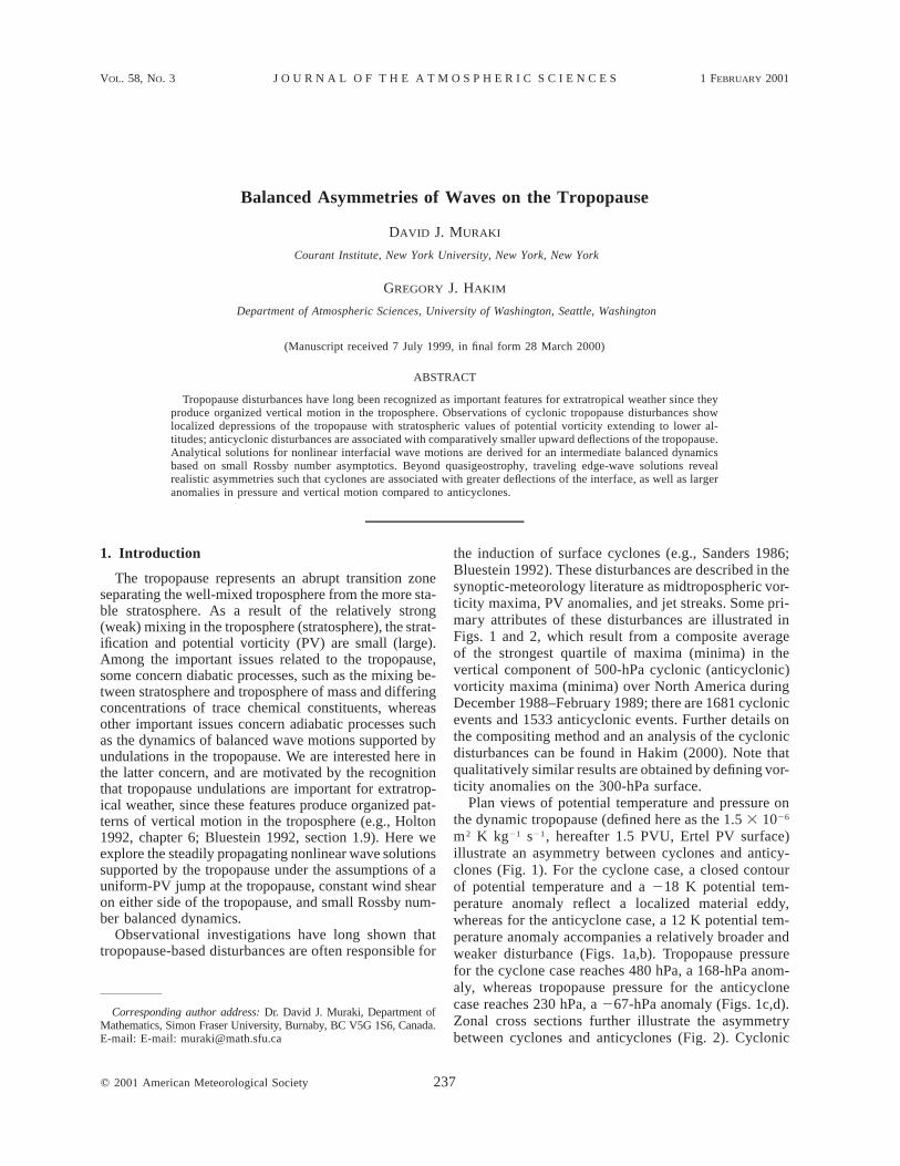
Plan views of potential temperature and pressure onthe dynamic tropopause (defined here as the 1.5 3 1026

m2 K kg21 s21, hereafter 1.5 PVU, Ertel PV surface)illustrate an asymmetry between cyclones and anticy-clones (Fig. 1). For the cyclone case, a closed contourof potential temperature and a 218 K potential tem-perature anomaly reflect a localized material eddy,whereas for the anticyclone case, a 12 K potential tem-perature anomaly accompanies a relatively broader andweaker disturbance (Figs. 1a,b). Tropopause pressurefor the cyclone case reaches 480 hPa, a 168-hPa anom-aly, whereas tropopause pressure for the anticyclonecase reaches 230 hPa, a 267-hPa anomaly (Figs. 1c,d).Zonal cross sections further illustrate the asymmetrybetween cyclones and anticyclones (Fig. 2). Cyclonic

238 VOLUME 58J O U R N A L O F T H E A T M O S P H E R I C S C I E N C E S

FIG. 1. Plan views of tropopause potential temperature (a), (b) and tropopause pressure (c), (d) for upper-tropospheric cyclones (a), (c)and upper-tropospheric anticyclones (b), (d). Mean (anomaly) potential temperature values are given by thick (thin) contours every 5 K (4K) with negative values dashed. Pressure contours are given every 25 hPa.

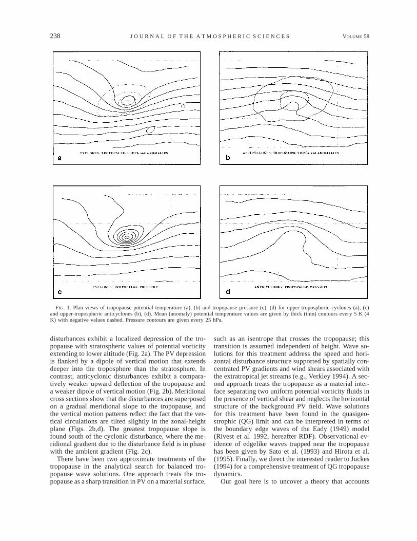
disturbances exhibit a localized depression of the tro-popause with stratospheric values of potential vorticityextending to lower altitude (Fig. 2a). The PV depressionis flanked by a dipole of vertical motion that extendsdeeper into the troposphere than the stratosphere. Incontrast, anticyclonic disturbances exhibit a compara-tively weaker upward deflection of the tropopause anda weaker dipole of vertical motion (Fig. 2b). Meridionalcross sections show that the disturbances are superposedon a gradual meridional slope to the tropopause, andthe vertical motion patterns reflect the fact that the ver-tical circulations are tilted slightly in the zonal-heightplane (Figs. 2b,d). The greatest tropopause slope isfound south of the cyclonic disturbance, where the me-ridional gradient due to the disturbance field is in phasewith the ambient gradient (Fig. 2c).

There have been two approximate treatments of thetropopause in the analytical search for balanced tro-popause wave solutions. One approach treats the tro-popause as a sharp transition in PV on a material surface,

such as an isentrope that crosses the tropopause; thistransition is assumed independent of height. Wave so-lutions for this treatment address the speed and hori-zontal disturbance structure supported by spatially con-centrated PV gradients and wind shears associated withthe extratropical jet streams (e.g., Verkley 1994). A sec-ond approach treats the tropopause as a material inter-face separating two uniform potential vorticity fluids inthe presence of vertical shear and neglects the horizontalstructure of the background PV field. Wave solutionsfor this treatment have been found in the quasigeo-strophic (QG) limit and can be interpreted in terms ofthe boundary edge waves of the Eady (1949) model(Rivest et al. 1992, hereafter RDF). Observational ev-idence of edgelike waves trapped near the tropopausehas been given by Sato et al. (1993) and Hirota et al.(1995). Finally, we direct the interested reader to Juckes(1994) for a comprehensive treatment of QG tropopausedynamics.

Our goal here is to uncover a theory that accounts

1 FEBRUARY 2001 239M U R A K I A N D H A K I M

FIG. 2. Zonal (a), (b) and meridional (c), (d) cross sections of Ertel potential vorticity, potential temperature, and vertical motion throughupper-tropospheric cyclones (a), (c), and anticyclones (b), (d). Ertel PV contours are given by thick solid lines (0.75; 1; 1.25; 1.5; 1.75; 2; 3;4; 5; 6 PVU), and the heavy line (1.5 PVU) denotes the dynamical tropopause. Potential temperature values are given by thin lines every 5 K,and vertical motion values are given by medium lines every 0.25 Pa s21 (negative values dashed). Note that 1 PVU 5 1026 K m2 kg21 s21.

for the prominent cyclone–anticyclone asymmetries pre-sent in tropopause observations but absent in the extantQG theory. We follow the approach of RDF and Juckes(1994) and treat the tropopause as a free material in-terface subject to an Eady-type shear flow. The edge-wave approach of RDF is extended to include the next-order balance effects using the QG11 methodology de-veloped in Muraki et al. (1999, hereafter MSR). Thenonlinearities at next order represent the feedback ofQG interfacial structure into the wave dynamics andcapture the primary observational asymmetries betweenthe interface depressions and elevations illustrated inFigs. 1 and 2. Section 2 outlines the Boussinesq prim-itive equations (PE), which serve as a starting point inthis investigation, the reference atmosphere, and the in-terface conditions to be satisfied by the solutions. Insection 3, the primitive equations are reformulated interms of three QG1 potentials, similar to the approachtaken by MSR, and an asymptotic approximation is out-

lined. Nonlinear wave solutions are derived for flat andsloped tropopause conditions, and compared with ob-servations in sections 4 and 5, respectively. Conclusionsand opportunities for future research are described insection 6.

2. Model formulation

The formulation of the model equations proceeds intwo parts. First, a set of Boussinesq primitive equationsare developed for an atmosphere having uniform strat-ification. Second, two of these atmospheres are stackedvertically and separated by the tropopause interface; theupper layer has a stratospheric Eady base state, and thelower layer has a tropospheric Eady base state. A crucialaspect of this construction involves the proper treatmentof interface conditions at the tropopause.


a. Boussinesq primitive equations

The starting point for our analysis of tropopausewaves is a simple model for the midlatitude atmosphereas described by a Boussinesq equation set that also in-cludes the inviscid, hydrostatic, and f -plane assump-tions:

F FD u 2y fxFu 1 y 1 w 5 0, 1 f 5 2 ,x y z F F1 2 1 2 1 2Dt y u fy

Fg DuF F2 u 5 2f , 5 0, (1)zu Dt0

where

D ] ] ] ]F[ 1 u 1 y 1 w (2)

Dt ]t ]x ]y ]z

denotes the usual material derivative. The dependentvariables are the wind velocities uF, y , and w; the po-tential temperature uF; and the pressure f F. The su-perscript F indicates full values that include both a meanbackground part and a disturbance. Although the quan-tities f F and z will be referred to as pressure and height,strictly speaking they represent geopotential and a mod-ified height coordinate (Hoskins and Bretherton 1972).The coefficients f, g, and u0 are the Coriolis parameter,the gravitational constant, and a reference potential tem-perature, respectively.

The tropopause represents a boundary between a low-PV troposphere and a high-PV stratosphere. This con-figuration can be captured by modeling the atmosphereas a two-fluid system composed of two regions of con-stant PV that are separated by an internal free bound-ary—a material interface across which the discontinuityin PV is supported. The stratospheric and troposphericregions are distinguished by differences in their meanbackground states that are defined by exact Eady-shearsolutions of (1). Tropopause waves are disturbance so-lutions from this basic Eady-shear state.

b. Eady mean reference state

The Eady mean-state atmosphere is a steady solutionof the Boussinesq primitive equations (1). It representsan atmosphere having constant stratification and uni-form vertical shear:

1 1 gM 2 2 2 M 2f [ N z 2 flyz 2 flsy , u [ N z 2 fly,

2 2 u0

Mu [ l(z 1 sy), (3)

where N is the Brunt–Vaisala frequency and l is theshear rate. The additional parameter s is introduced inanticipation that a tilt of the uM 5 0 velocity surfacewill be useful for the construction of a two-layer at-mosphere (as in RDF). In the idealized tropopause rep-resentation, the distinction between stratosphere and tro-

posphere is defined through their representative valuesof N and l.

c. Scaling and nondimensionalization

For disturbances upon the Eady state (3), character-istic vertical and horizontal length scales are denotedby H and L, and horizontal velocity scales by V. Theassumption that the flow be near quasigeostrophic bal-ance requires the dimensionless conditions of small as-pect ratio, small Rossby number, and order-unity Burgernumber:

H Vd [ K 1, e [ K 1,

L fL

2NHB [ 5 O(1). (4)1 2fL

In addition, O(1) nondimensional shear and tropopause-slope parameters associated with the background shear(3) are defined and scaled as in RDF:

lH sL [ 5 O(1), s [ 5 O(1). (5)

V de

Note that the viability of these scalings [(4), (5)] forQG balance demands only that the atmosphere bestrongly stratified with respect to both Coriolis and shearinfluences ( f K N and l K N).

Nondimensionalization of the Boussinesq system (1)is based on the disturbance scales x, y ; L, and z ; H,and on the horizontal advection timescale t ; L/V. Fol-lowing Pedlosky (1987), the disturbance winds and ver-tical motion are scaled as

u 5 uF 2 uM ; V, y ; V, w ; edV, (6)

and the pressure and potential temperature disturbancescales are those of thermal-wind balance:

F Mf 5 f 2 f ; VfL,

gF Mu 5 (u 2 u ) ; VfL /H. (7)

u0

Note that all of the disturbance variables have beencarefully scaled to be independent of variations in theambient stratification N and shear parameter l, sincethese quantities are different in the stratosphere and tro-posphere.

d. Disturbance equations

Applying these nondimensionalizations to the Bous-sinesq system (1) results in the disturbance PE for theEady mean state:


u 1 y 1 ew 5 0x y z

Du2e 1 e L(sy 1 w) 2 y 5 2fxDt

Dye 1 u 5 2fyDt

2u 5 2fz

Du2 Ly 1 Bw 5 0, (8)

Dt

where the material derivative

D ] ] ] ][ 1 [L(z 1 esy) 1 u] 1 y 1 ew (9)

Dt ]t ]x ]y ]z

includes advection by the Eady shear. The dimensionlessexpressions for the Eady state (3) with disturbances are

1 B 1F 2 2f 5 z 2 Lyz 2 eLsy 1 f,

2 e 2

BF Fu 5 z 2 Ly 1 u, u 5 Lz 1 eLsy 1 u. (10)

e

Note that the O(1/e) leading terms in f F and uF embodythe strong stratification implied by the assumption ofsmall Rossby number. The nondimensionalized Ertel po-tential vorticity based on (10) is

F u FQ [ z 1 e= 3 y · (=u )

0

B5 2 eL(L 1 Bs) 1 Bq, (11)[ ]e

which is decomposed into a contribution from the Eadymean state plus a disturbance potential vorticity termdenoted by q. The Eady contribution, although large, isuniform in both the stratosphere and troposphere, andprovides the PV contrast primarily through a jump inthe stratification B. It is also clear that only the distur-bance portion of the potential vorticity (PV),

1q 5 y 2 u 1 ux y z1 2B

e1 [(y 2 u 2 eLs)u 2 y u 1 u ux y z z x z yB

1 L(u 2 u )], (12)y z

is dynamically relevant. Its evolution is governed bymaterial conservation,

Dq5 0, (13)

Dt

and unless stated otherwise, the term PV will be re-served for this disturbance value q.

e. A tropopause atmosphere

Following RDF, the Eady basic state allows for theconstruction of a tropopause base state by introducinga jump in the values of Burger number B and shear L(and hence, a jump in PV), which supports an internalmaterial surface. By the scalings (4) and (5), the PE (8)conveniently apply for both stratosphere and tropo-sphere with the appropriate values of B and L. Strato-spheric values are denoted by Bs, Ls and troposphericvalues by Bt, Lt. To exploit this notational symmetryand to simplify the presentation, the bold script s andt will be omitted whenever the context is unambiguous.

For the undisturbed atmospheric state, the height ofthe tropopause (zi) is located at the level with zero hor-izontal wind shear, zi 1 esy 5 0; see (10). The strato-sphere resides above this level, z . zi, and the tropo-sphere below, z , zi. Imposing continuity of the un-disturbed pressure and temperature (10) at z 5 zi, thecontrast in background parameters requires

L 2 Lt ss 5 , (14)B 2 Bs t

which implies a unique value for the weak meridionaltilt of the tropopause [cf. RDF, their Eq. (24)].

It will prove useful in the interpretation of the edge-wave dispersion relation to note that the equivalent me-ridional gradient in pseudo-PV (Pedlosky 1987, p. 358)of the basic state can be written as

eq 2 F]Q ] u 2 u L Lt s5 ø 2 d(z 1 esy), (15)1 2 1 2]y ]z]y B B Bt s

where d(z 1 esy) is the Dirac delta function acting atthe tropopause. Although the tropopause slope s be-comes negative for Ls/Lt . 1, a negative meridionalPV gradient requires the stronger condition Ls/Lt .Bs/Bt . 1, which reflects the considerable dynamicalinfluence exerted by the stratification difference acrossthe interface.

Two special reference atmospheres are considered:one having a flat tropopause, in the case of uniformshear (Ls 5 Lt), and the other a sloped tropopause, inthe case without stratospheric shear (Ls 5 0; as in RDF).Meridional profiles of full potential temperature uF forboth reference atmospheres are shown in Fig. 3. Theexact compensation by the tropopause tilt for the zerostratospheric shear is evident from the continuity of theisentropes in Fig. 3b.

f. Interface conditions

As constructed above, the reference tropopause sat-isfies continuity of pressure and temperature, in additionto the interface being a material surface within the shearflow. These three properties of the interface must bemaintained when disturbance flow and tropopause de-formation are included. The major technical difficulty


FIG. 3. Meridional cross section of potential temperature for (a) flat and (b) sloped undisturbedtropopause position. Potential temperature values are given by thin lines every 5 K. The heavyline denotes the undisturbed tropopause interface. Parameters common to both cases are e 50.1, Bs 5 4, and Bt 5 1. The Eady shear parameters are Ls 5 0, Lt 5 1 for the slopedtropopause, and Ls 5 Lt 5 1 for the flat tropopause.

involves the participation of the tropopause as a dy-namical surface, which distinguishes the regions of dif-fering B and L in the PE (8). The equations for theinterface conditions are best described in a coordinatesystem that naturally slopes with the undisturbed tro-popause. Prior to adjusting the coordinates and outliningthe interface matching conditions for the disturbed tro-popause, the QG11 reformulation of the PE (8) is pre-sented.

3. QG11 tropopause wave asymptotics

a. QG1 reformulation of the primitive equations

The tropopause wave solutions of the disturbance PE(8), which include the next-order corrections beyondQG, are constructed following the QG1 methodology,a systematic asymptotic approach to quasigeostrophicbalance (MSR). This method is applied here within thecontext of the above PE (8), taking explicit account ofthe Burger number, B. The QG1 method generalizes thefamiliar QG streamfunction representation to a three-potential representation:

1 1y 5 F 2 G , 2u 5 F 1 F ,x z y zB B

u 5 F 1 G 2 F , eBw 5 F 1 G . (16)z x y x y

The PE (8) are then exactly equivalent to the sequenceof elliptic inversions for the potentials (F, F, G):

e2¹ F 5 q 2 [(y 2 u )u 2 y u 1 u uB x y z z x z yB

1 L(u 2 u 2 esu )]y z z

Du Dy2¹ F 5 e 2 1 1 LyB x1 2 1 2[ ]Dt Dt

x z

Du Du2¹ G 5 e 2 2 1 L(y 2 esy 2 ew ) ,B y z z1 2 1 2[ ]Dt Dt

y z

(17)

where the Laplacian operator is modified by the strat-ification B:

2 2 2] ] 1 ]2¹ [ 1 1 . (18)B 2 2 2]x ]y B ]z

Inclusion of the PV evolution equation (13) completesthe reformulation of the PE in terms of QG1 potentials.It is emphasized that the above QG1 system of equations[(16), (17), (13)] constitutes an exact reformulation ofthe disturbance PE (8). This particular form of the PEhas been crafted to enable a straightforward truncationto QG and its perturbative corrections. For complete-ness, we note that unbalanced motions, such as gravitywaves, reside within (17), and can be isolated by a ju-diciously chosen timescale and expansion procedure(MSR).


The QG11 balanced system is constructed by assum-ing a perturbation solution based upon the small Rossbynumber (e) expansion:

0 1 2 1 2F 5 F 1 eF 1 O(e ), F 5 eF 1 O(e ),1 2G 5 eG 1 O(e ), (19)

which allows for an iterative inversion of correctingpotentials using (17). The boundary and interface con-ditions for these inversions are obtained from physicalconditions in terms of primitive variables. Specific tothis tropopause analysis, the QG11 asymptotic procedurerequires an additional alteration that is dictated by thetilt of the tropopause and involves a change to a slopedcoordinate frame.

b. Tropopause coordinates

The tropopause wave is obtained as a stationary wavesolution in a zonally propagating frame. This wave so-lution must possess lateral periodicity in the directionsparallel to the reference tropopause surface. With thetilted tropopause (s ± 0), it proves useful to expressthe spatial structure in terms of a (slightly) skewed co-ordinate system where the vertical coordinate is refer-enced to the undisturbed (tilted) tropopause. This mo-tivates a change to tropopause coordinates, as definedby a translating and O(e)-skewed frame:

x 5 x 2 ct, y 5 y, z 5 z 1 esy, t 5 t, (20)

where c is the zonal wave speed. In this moving frame,traveling wave solutions are independent of t . Most im-portant, the reference tropopause now resides at z i 5 0.

c. The tropopause as a free-boundary interface

The tropopause waves are essentially two edge wavestrapped on an isolated internal interface. In addition tolateral periodicity, wave disturbances are also assumedto decay in the vertical away from the tropopause z →6`. At the tropopause, the physical conditions to besatisfied are continuity of (full) pressure and tempera-ture, and dynamics of the tropopause as a material sur-face.

The disturbed tropopause is described as a surfacethat is displaced from the reference tropopause:

z i 5 eh(x , y , t). (21)

As noted in RDF and Juckes (1994), this weak O(e)scaling of the tropopause displacement is a requirementfor the temperature disturbances to be consistent withQG balance. Dimensionally, this means that this analysisfor tropopause waves will be strictly valid only whenthe height of the tropopause disturbances is smaller thanthe Rossby height as defined by the ambient stratifi-cation. The interface continuity conditions on f F anduF (10), in terms of tropopause coordinates (20) can bewritten

s1

2 sf 1 Beh 5 {u 1 Bh} 5 0, (22)t5 62 t

where the bold s, t notation indicates subtraction ofstratospheric and tropospheric values at the tropopause.

The third condition is that the tropopause interfacerepresents a material surface with respect to both theupper and lower flows:

iD

[z 2 eh(x, y, t)]5 6Dti5 e{sy 1 w 2 h 2 (eLh 1 u 2 c)h 2 yh }t x y

5 0, (23)

where the superscript i indicates evaluation on the tro-popause in either the stratosphere or the troposphere.This interface condition is required since the tropopausedisplacement, h(x , y , t), is determined as part of thesolution. The PE (8), or equivalently QG1 (13), (16),(17), with boundary and interface conditions (22), (23)represent a complete specification of a free-boundaryinterface problem for the dynamics of the tropopause.

Specific to the tropopause wave, it proves convenientto combine (23) with the thermodynamic (u advection)equation in the PE (8) to give

u u L 1 sB(eLh 1 u 2 c) 1 h 1 y 1 h 2 y5 1 2 1 2[ ]B B B yx

ie

1 (w 1 sy)u 5 0,z6B(24)

where the restriction to a steady, t-independent wavehas also been made.

Finally, the weak displacement assumption (z i K 1)also allows the evaluation of the interface quantities thatarise in the conditions (22), (24) through a Taylor ex-pansion. For instance, the value of a functionf (x , y , z , t) on the interface z i 5 eh(x , y , t) has the Tay-lor representation

f (x, y, z , t ) ; f (x, y, 0, t ) 1 ehf (x, y, 0, t )i z

12 21 e h f (x, y, 0, t ) 1 · · · , (25)z z2

so that all tropopause conditions can be expressed interms of z 5 0 quantities. Finally, it should be notedthat the formulation (21) also assumes lateral gradientsof the tropopause h(x , y , t) to be O(1), which precludesthe validity of this analysis for tropopause folds.

4. QG1 tropopause wave solutions

Using QG theory, RDF successfully showed that asimple single-mode tropopause wave can be describedusing two copropagating Eady edge waves that decayaway from the tropopause interface. More generally, this


QG wave corresponds to a leading-order, nonlinear so-lution of the PE (8) that is characterized by uniforminterior PV and is steady with respect to a frame movingwith speed c. In a manner similar to that of the QG11

edge wave (MSR), here we derive the next-order tro-popause wave solution whose nonlinear corrections dis-play cyclone–anticyclone asymmetry.

a. QG11 perturbation expansions

In tropopause coordinates, the next-order potentialrepresentations (16) are

10 1 1 2y 5 F 1 e F 2 G 1 O(e )x x z1 2B

10 1 1 0 22u 5 F 1 e F 1 F 1 sF 1 O(e )y y z z1 2B0 1 1 1 2u 5 F 1 e(F 1 G 2 F ) 1 O(e )z z x y

1 1Bw 5 F 1 G 1 O(e), (26)x y

which, in the flat case (s 5 0), recovers (16). In addition,the tropopause displacement is also expressed as a per-turbation series:

h(x , y) 5 h0(x , y) 1 eh1(x , y) 1 O(e2), (27)

which allows the interface conditions (22), (24) to besatisfied expansions in Rossby number. Last, the onlyimpact of the skewed coordinates (20) at next order inthe QG1 potential inversions (17) is an extra term inthe Laplacian operator:

2 2 2 2] ] 1 ] ]2 2¹ 5 1 1 1 e2s 1 O(e ). (28)B 2 2 2]x ]y B ]z ]y]z

b. Leading-order QG tropospause wave

The leading-order wave is expressed solely in termsof F0(x , y , z) (26) in which the potential representation(16) reduces to the familiar geostrophic relations

y ; , 2u ; , u ; , f ; F0,0 0 0F F Fx y z (29)

and F0 is a solution to the zero-PV inversion (12):

2 10 0 0 0¹ F [ F 1 F 1 F 5 0. (30)B x x y y z zB

Horizontally periodic Eady solutions are single-modeupper/lower waves given by

s: A coskx cosly exp(2mÏB z )s s0F 5 (31)5t: A coskx cosly exp(1mÏB z ),t t

where m2 5 k2 1 l2, and the sign of the exponent ischosen for decay away from the tropopause z → 6`.Note that the s, t solutions of F0 (31) are defined byregions above and below the displaced tropopause po-sition z 5 eh(x , y).

The relative amplitudes As and At, the leading-ordertropopause height h0(x , y), and the wave speed c aredetermined through the interface conditions (22), (24).The weak displacement assumption permits leading-or-der application of the tropopause conditions at z 5 0,as O(e) errors in the interface evaluations (25) are de-ferred to next order. Thus by virtue of the continuity ofleading-order pressure (22), the amplitudes As 5 At 5A are the same for both upper and lower solutions. Theleading-order terms of the material condition (24) canbe manipulated into a zero-Jacobian condition

i00u L 1 sB

0 0J F 1 cy, 1 h 2 y 5 0, (32)5 1 2 6[ ]B B

where J( f, g) [ 2 is the Jacobian derivative;f g f gx y y x

the bold i0 superscript denotes evaluation on z 5 0. Fora periodic wave, the Jacobian can only vanish when thetwo arguments are proportional. Since the nonlinearityin Jacobian (32) exactly cancels, the remaining interfaceconditions (32) and (22) reduce to

i00L 1 sB u

0 0F 1 c 1 h 5 051 2 1 26B B0 0 s0{u 1 Bh } 5 0, (33)t0

where the first relation is really two conditions, as itmust hold at the interface for both the stratospheric andtropospheric solutions. The bold scripts s0 and t0 denotethat the difference between stratospheric and tropo-spheric values are evaluated at z 5 0.

Quasigeostrophic solutions derive from substituting(31) into (33). The second condition in (33) gives therelationship between the interface displacement and thestreamfunction,

m0 0h (x, y ) 5 F (x, y, 0)

ÏB 2 ÏBs t

0[ C F (x, y, 0), (34)h

which is equivalent, for Ls 5 0, to the corrected RDFformula noted by Juckes [1994, Eqs. (3.9) and (3.10)].The proportionality between tropopause height and QGstreamfunction, Ch, is independent of the backgroundshear, and as expected, is singular in the limit of van-ishing interface (Bs → Bt). The first condition in (33)gives the dispersion relationship,

211 L L 1 1t s 2c 5 2 1 1 O(e ), (35)1 21 2m B B ÏB ÏBt s s t

which again reduces to the RDF solution when Ls 5 0.Furthermore, the direct relationship in (35) betweenwave speed and base-state pseudo-PV gradient (15)highlights the qualitative similarity between tropopauseedge waves and classic barotropic Rossby waves. Notealso that in the limit Bs or Bt → `, (34) and (35) reduceto QG edge waves trapped on a rigid surface (Gill 1982).


The correspondences presented here are consistent withJuckes’s (1994) more general observation of the dy-namical equivalence between the QG tropopause andsurface quasigeostrophy (Held et al. 1995). Last, al-though in general one might expect the wave speed cto be corrected at next order, we state here for simplicity(anticipating the QG11 construction) that the correctionat O(e) is exactly zero.

Finally, using the thermodynamic relation, the lead-ing-order vertical motion is given by

Bw0 5 [Ly 0 1 (c 2 Lz) ]0ux

5 [LF0 1 (c 2 Lz) .0u ]x (36)

c. QG11 wave corrections

The extension of the tropopause wave to next orderin Rossby number involves solving for the potentialsF1, F 1, G1 subject to the next-order interface conditions.The most important results of this calculation are thecorrections that are nonlinear in the wave amplitude, asthese terms are responsible for the cyclone–anticycloneasymmetries. The major complication lies in the com-plete solution of F1, where a homogeneous boundarycorrection must be determined. A careful statement1Fof this difficulty is given below, and some additionaldetails of the calculation are deferred to appendix B.

The potentials F1, F 1, and G1 are obtained by next-order Poisson inversions (17) in tropopause coordinates(20):

2 1 11 0 2 0 2 0 2¹ F 5 (F ) 1 (F ) 1 (F )B x z y z z z[ ]B B

202 (L 1 sB)Fy zB

21 0 0 0¹ F 5 2J(F , F ) 1 2LFB z x x x

21 0 0 0¹ G 5 2J(F , F ) 1 2LF , (37)B z y x y

where extra terms in the F1 equation are generated bythe rotated Laplacian (28). All three potentials can beexpressed almost completely in terms of derivatives and(indefinite) integrals of the QG solution:

11 0 2 0 1˜F 5 (F ) 2 (L 1 sB)zF 1 Fz y2B

z

1 0 0 0 0 0F 5 F F 1 LBz F 1 (cu 1 LF )y z E x x1 2z

1 0 0 0G 5 2F F 1 LBz F , (38)x z E x y

with appropriate choices taken for B, L, and F0 (31) inthe stratosphere and troposphere (for notational sim-plicity, the formal dz is dropped from the integral op-erator). The final term for F 1 is a homogeneous solution,

which is necessary for QG11 consistency with mass con-tinuity (16):

1 5 Bw0,1 1F Gx y (39)

where w0 is given by (36). At this point, it remains onlyto determine a homogeneous solution , which is nec-1Fessary to satisfy the physical conditions at the interface(22), (24).

The QG11 pressure is obtained from a vertical inte-gration of the next-order hydrostatic balance 5 u1,1f z

where u1 is constructed using the QG11 potentials (38):z1 2

1 1 0 2 0 0f 5 F 2 ¹ (F ) 2 cF 2 L F , (40)H y E y4

and 5 1 .2 2 2¹ ] ]H x y

There are two conditions that define the homogeneouscontribution . The first condition comes from con-1Ftinuity of the O(e) contributions of full pressure on thetropopause (22):

s0z 11 0 0 2F 2 L F 5 (B 2 B )(h ) , (41)E y s t1 2 2

t0

where the apparent sign change of the right side withrespect to (22) follows from the inclusion of the deferredO(e) Taylor correction (25) of the leading-order pressuref 0(x , y , z i) evaluated at z i ; eh0.

A second condition on is given by the O(e) terms1Fof the interface condition (24). Its derivation requires aconsiderable amount of manipulation, and the essentialdetails are deferred to appendix A. Specifically, for thetropopause wave (31):

s0z1 ] (L 1 sB)1 0˜1 F 2 L FE y5 1 21 26B ]z c t0

20 25 (C ¹ 1 C )(F ) 1 C , (42)1 H 2 3

where the three C constants are also defined in appendixA. Boundary conditions (41) and (42) determine a ho-mogeneous solution of the form1F

z

1 1 0 1˜ ˜F 5 f 1 L F 1 F , (43)nl E y nl

where the nonlinear part consists of a constant and1Fnl

second harmonics only; the full solution is given inappendix B. Note that the linear part of (43) is not1Funiquely determined by the boundary conditions but bydemanding that the solution give the QG11 edge wavesof MSR in the limit of either Bs or Bt → `. Last, thecorrection to the tropopause displacement follows im-mediately from next-order continuity of potential tem-perature (22):

1 1 0 0 s0(B 2 B )h 5 2{u 1 h u } , (44)s t z t0

where the second right-side term is a Taylor correctionfrom the tropopause displacement.


TABLE 1. Values for scaling parameters, derived nondimensional quantities, and derived dimensional quantities.

Dimensional quantities Nondimensional quantities Dimensional scales

L 1000 km eV

f L 0.1 tL

Vø27.8 h

H 10 km dH

L 0.01 s eds 0 or ø20.333 m km21

V 10 m s21 Bs

2N Hs1 2f L 4 f Vf L 103 m2 s22

f 1024 s21 Bt

2N Ht1 2f L 1 p r0Vf L 10 hPa

Ns 4 3 1022 s22 Lt

lH

V 1 uVf L u0

H g 3K

Nt 1 3 1022 s22 Ls 1 or 0 w edV 1 cm s21

l 1 m s21 km21 sL 2 Lt s

B 2 Bs t

0 or 21

3

u0

g 30 K s2 m21

r0 1 kg m23

FIG. 5. Plan view of tropopause potential temperature comparing(a) QG and (b) QG11 solutions for the sloped case. Full values uF

are given by thick solid lines every 5 K, and disturbance values uare given by thin lines every 4 K, with negative values dashed.

FIG. 4. Plan view of tropopause potential temperature comparing(a) QG and (b) QG11 solutions for the flat case. Full values uF aregiven by thick solid lines every 5 K, and disturbance values u aregiven by thin lines every 4 K, with negative values dashed.

5. The tropopause waves

Here we discuss the structure of the tropopause wavesolutions for both flat- and sloped-tropopause basicstates. All figures are plotted in physical coordinateswith typical dimensional values that are given in Table1. The tropopause maps (Figs. 4–7, 10) represent a fullwavelength in y and a half wavelength in x. Tropopausevalues are approximated at the displaced interface po-sition using the Taylor expansion (25). In the verticalprofiles (Figs. 8, 9, 10), discontinuities in the contoursacross the tropopause appear for two reasons. First, al-

though the interface-normal velocity is continuous atthe interface, the individual wind components are un-constrained. This fact accounts for the misaligned con-tours of y in Fig. 10, and to a lesser degree w in Fig.8. Second, although full temperature and pressure arecontinuous at the interface (22), there are systematicerrors associated with the asymptotic truncation to O(e)in QG and O(e2) in QG11. The tropopause wave solu-tions shown here, with Rossby number e 5 0.1, aresquare waves with k 5 l 5 1 and amplitude A 5 1.0,except where A 5 0.7 in Fig. 11. For simplicity, cy-clone–anticyclone asymmetry is quantified below as the


FIG. 6. Plan view of tropopause height comparing (a) QG and (b)QG11 solutions for the flat case. Disturbance values h are given every500 m.

FIG. 7. Plan view of tropopause height comparing (a) QG and (b)QG11 solutions for the sloped case. Full values 2sy 1 h are givenby thick solid lines every 600 m, and disturbance values h are givenby thin lines every 500 m, with negative values dashed.

absolute value of the ratio of cyclone to anticycloneextreme values; all aspects of the QG solutions have anasymmetry ratio of unity.

The tropopause potential temperature field for the QGand QG11 flat-tropopause solutions are shown in Figs.4a and 4b. Cyclonic and anticyclonic cells are sym-metric for the QG wave, whereas the cyclonic cell isnotably stronger for the QG11 wave, with an asymmetryratio of 2.875. Furthermore, the contributions from thesecond harmonics produce a more localized, nearly axi-symmetric structure for the QG11 cyclone in contrast tothe broader, more squarelike structure for the QG11 an-ticyclone. The sloped-tropopause case in Fig. 5 is sim-ilar to the flat-tropopause case, except for an asymmetryof 1.89 and stronger (weaker) gradients in the full po-tential temperature field to the south (north) of the QG11

cyclone (anticyclone). An enhanced gradient region issuggestive of upper-level fronts, which typically occurnear steeply sloped regions of the tropopause (e.g., Key-ser and Shapiro 1986). Two closed contours in the fullpotential temperature field signify a region of trapped,vortical fluid in the QG11 cyclone, whereas the QG wavehas open, wavelike, material contours. Comparing ob-servations with the QG11 solution shows that the QG11

solution captures the qualitative properties of the cy-clone–anticyclone asymmetry, as well as the materialeddy and wavelike properties of the cyclone and anti-cyclone, respectively (cf. Fig. 5b with Figs. 1a,b).

Cyclone–anticyclone asymmetry is dramatically il-lustrated in the tropopause height perturbations, whichhave an asymmetry of 3.86 for the flat tropopause waves(Fig. 6). The height asymmetry for the sloped-tropo-pause solutions is 2.22, and this solution compares morefavorably with observations since the ambient gradientof tropopause height is included (cf. Fig. 7b with Figs.

1c,d; note that tropopause pressure and height are close-ly correlated). Furthermore, a significant improvementin the sloped solution over the flat solution is the re-duction of second-harmonic contributions in the cor-rections to the former, which removes a local minimumfrom the anomaly height field at the center of the flatanticyclone (Fig. 6b).

A zonal cross section through the waves highlightsthe profile of the disturbed interface, with an enhancedcyclone and a flattened anticyclone for the QG11 relativeto the QG solution (Fig. 8); note the qualitatively similarbehavior in the observations (Figs. 2a,b). Vertical mo-tions are damped above the interface and reach theirlargest magnitude below the interface for both QG andQG11 solutions. A notable difference between the QGand QG11 solutions is slightly stronger vertical motionsthat are concentrated toward the cyclone center in amanner similar to the dipole of vertical motion notedin observations (cf. Fig. 8b with Fig. 2a). This behaviormay be explained by the dynamic interface condition,which requires greater vertical motions to elevate anddepress the interface near the QG11 cyclonic interfacedeflection. Note that since w scales with the laterallength scale as L22, solutions for higher wavenumbersk, l exhibit considerably larger vertical motions whoseextrema are much closer to the interface. Since the di-mensional horizontal scale of these waves is ;3000 km(half wavelength), this tendency would be more in linewith the observations in Figs. 2a,b where the horizontalscale is significantly less at ;1000 km.

The potential temperature lines in the tropospherebulge upward in the cyclone and downward in the an-ticyclone in a manner similar to observations (cf. Figs.8 and 2a,b), and as one would expect from PV reasoningbased on local cyclonic and anticyclonic PV anomalies


FIG. 8. Zonal cross section of full potential temperature uF and vertical motion w comparing(a) QG and (b) QG11 solutions for the sloped case. Potential temperature is given by thin solidlines every 5 K, and vertical motion is given by thick lines every 1 mm s21, with negativevalues dashed. The heavy line denotes the tropopause interface.

FIG. 9. Meridional cross section of full potential temperature uF comparing (a) QG and (b)QG11 solutions for the sloped case. Potential temperature is given by thin solid lines every 5K. The heavy line denotes the tropopause interface. The vertical motion w is identically zeroin this cross section.


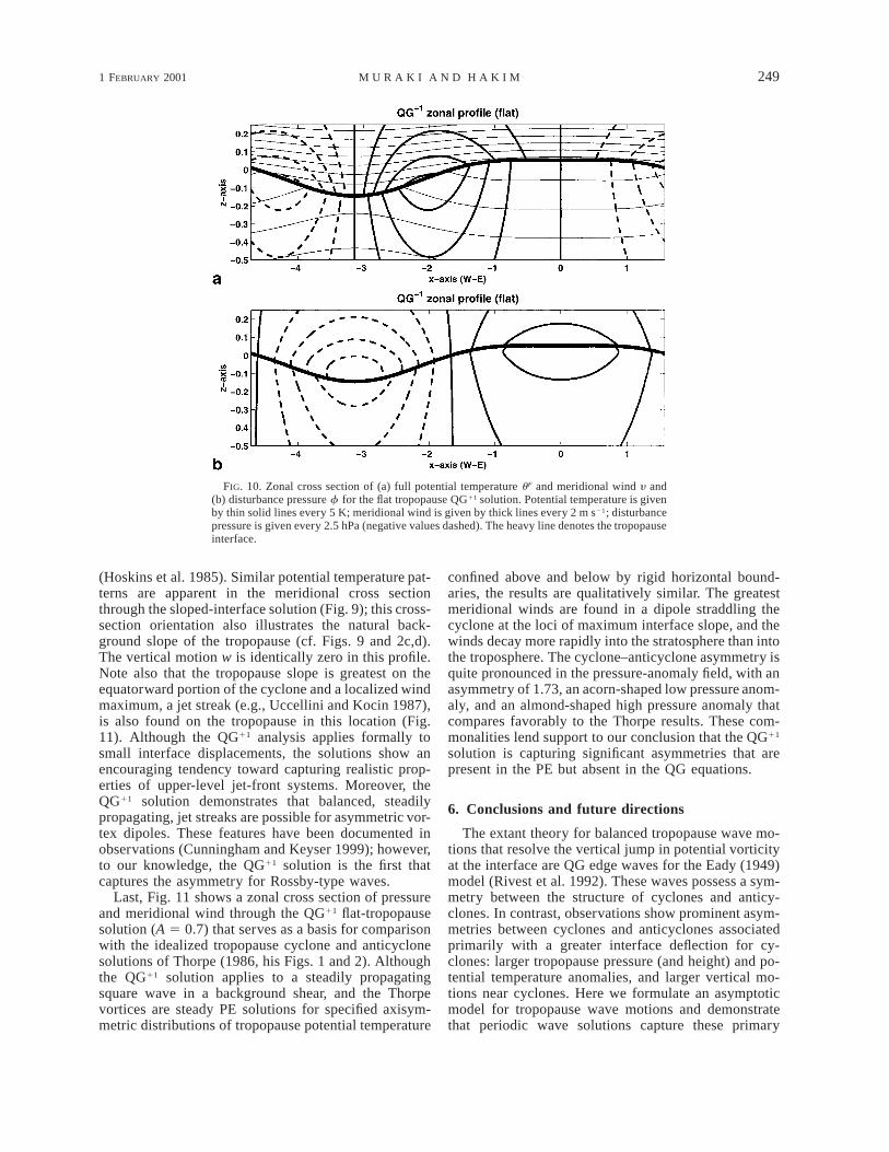
FIG. 10. Zonal cross section of (a) full potential temperature uF and meridional wind y and(b) disturbance pressure f for the flat tropopause QG11 solution. Potential temperature is givenby thin solid lines every 5 K; meridional wind is given by thick lines every 2 m s21; disturbancepressure is given every 2.5 hPa (negative values dashed). The heavy line denotes the tropopauseinterface.

(Hoskins et al. 1985). Similar potential temperature pat-terns are apparent in the meridional cross sectionthrough the sloped-interface solution (Fig. 9); this cross-section orientation also illustrates the natural back-ground slope of the tropopause (cf. Figs. 9 and 2c,d).The vertical motion w is identically zero in this profile.Note also that the tropopause slope is greatest on theequatorward portion of the cyclone and a localized windmaximum, a jet streak (e.g., Uccellini and Kocin 1987),is also found on the tropopause in this location (Fig.11). Although the QG11 analysis applies formally tosmall interface displacements, the solutions show anencouraging tendency toward capturing realistic prop-erties of upper-level jet-front systems. Moreover, theQG11 solution demonstrates that balanced, steadilypropagating, jet streaks are possible for asymmetric vor-tex dipoles. These features have been documented inobservations (Cunningham and Keyser 1999); however,to our knowledge, the QG11 solution is the first thatcaptures the asymmetry for Rossby-type waves.

Last, Fig. 11 shows a zonal cross section of pressureand meridional wind through the QG11 flat-tropopausesolution (A 5 0.7) that serves as a basis for comparisonwith the idealized tropopause cyclone and anticyclonesolutions of Thorpe (1986, his Figs. 1 and 2). Althoughthe QG11 solution applies to a steadily propagatingsquare wave in a background shear, and the Thorpevortices are steady PE solutions for specified axisym-metric distributions of tropopause potential temperature

confined above and below by rigid horizontal bound-aries, the results are qualitatively similar. The greatestmeridional winds are found in a dipole straddling thecyclone at the loci of maximum interface slope, and thewinds decay more rapidly into the stratosphere than intothe troposphere. The cyclone–anticyclone asymmetry isquite pronounced in the pressure-anomaly field, with anasymmetry of 1.73, an acorn-shaped low pressure anom-aly, and an almond-shaped high pressure anomaly thatcompares favorably to the Thorpe results. These com-monalities lend support to our conclusion that the QG11

solution is capturing significant asymmetries that arepresent in the PE but absent in the QG equations.

6. Conclusions and future directions

The extant theory for balanced tropopause wave mo-tions that resolve the vertical jump in potential vorticityat the interface are QG edge waves for the Eady (1949)model (Rivest et al. 1992). These waves possess a sym-metry between the structure of cyclones and anticy-clones. In contrast, observations show prominent asym-metries between cyclones and anticyclones associatedprimarily with a greater interface deflection for cy-clones: larger tropopause pressure (and height) and po-tential temperature anomalies, and larger vertical mo-tions near cyclones. Here we formulate an asymptoticmodel for tropopause wave motions and demonstratethat periodic wave solutions capture these primary


FIG. 11. Plan view of tropopause height and total wind speed forthe sloped case. Full values 2sy 1 h are given by thin solid linesevery 600 m, and total wind speed contours are given by thick solidlines (15, 17.5, 20 m s21); a uniform background zonal wind speedof 10 m s21 has been added to the solution.

asymmetries. This analysis combines an extension ofthe QG approximation to the primitive equations (QG11)following Muraki et al. (1999) with an expansion forthe tropopause position that asymptotically satisfies con-tinuity of pressure, temperature, and a dynamic interfacecondition. At leading order, the QG waves of the afore-mentioned extant theory are recovered. At next order,cyclone–anticyclone asymmetries emerge that comparefavorably to observations. These asymmetries arise pri-marily due to the nonlinear feedback of QG displace-ments into the QG11 wave dynamics, which are greatlyinfluenced by the enhanced stability of the stratosphericbase state.

Two basic states are considered: a flat tropopause as-sociated with uniform shear in the troposphere andstratosphere, and a sloped tropopause associated withzero shear in the stratosphere. Solutions for both basicstates capture the primary asymmetries noted in obser-vations, including the larger tropopause potential tem-perature and height perturbations associated with cy-clones. For a wave amplitude of A 5 1.0, the contri-butions from just the second-harmonic corrections in

the solution produce a localized cyclonic vortex withclosed material lines as compared to a broader anticy-clone with square wavelike open material lines. Al-though vertical motions are maximal below the interfacefor both the QG and QG11 wave solutions, the next-order corrections produce a stronger, more localizedstructure of vertical motion beneath the cyclone. Theselarger vertical motions are completely consistent withgreater tropopause height deformations associated withthe cyclonic part of the wave.

A noteworthy feature of the wave solution is the lackof tilt in its zonal profile despite the background verticalshear; this is consistent with the fact that a neutral (non-growing) traveling wave cannot exchange energy withthe shear flow (e.g., Pedlosky 1987, section 7.3). How-ever, observations show a tilt of the vertical circulationin the zonal-height plane (Fig. 2a). This tilt in the ob-servations could be due to a number of reasons, amongthem meridional velocity shears, time-dependent aver-age growth (decay) of the cyclones (anticyclones), or aslight NW to SE bias of the mean jet stream.

Localized wind speed maxima, jet streaks, are cap-tured by both the QG and QG11 solutions equatorwardof the cyclone disturbance. An important characteristicat next order is the cyclone–anticyclone asymmetry thatis often noted in observations of jet streaks associatedwith vortex dipoles. A novel aspect of these next-ordersolutions is that the symmetry breaking to a dipole witha strong cyclone and a weak anticyclone follows nat-urally from a bias within the QG11 dynamics.

In addition, the next-order solutions compare favor-ably with the primitive equation PV-inversion solutionsof Thorpe (1986) for steady vortices. The close corre-spondence between our solutions, observations, andThorpe’s solutions supports our conclusion that the im-portant asymmetries contained in the primitive equa-tions are well represented within the QG11 theory. Thiscorroboration provides an incentive to conduct morecareful comparisons between the solutions and obser-vations. One opportunity would be to take these tro-popause wave solutions as an initial basis for correla-tions between various disturbance amplitudes, such asanomalies in, for example, potential temperature, pres-sure, and vorticity, to compare with similar statisticsobtained from observations. Another avenue for inves-tigation would be to extract particle trajectories fromthese more realistic tropopause wind fields for the pur-pose of understanding mechanisms for vertical transporttoward the tropopause.

The sloped-tropopause solution introduces the naturalmeridional tilt of the tropopause that is absent in theflat solutions. One apparent defect of the flat solutionis a local minimum in the height anomaly field locatedat the center of the anticyclone; this feature is absentin the sloped solution (Fig. 7). In the sloped solution,the steepest gradients of tropopause height are foundequatorward of the cyclone disturbance. This feature isassociated with enhanced gradients of tropopause po-


tential temperature, and is reminiscent of an upper-levelfront. It has been noted that a limitation of this asymp-totic model (due to the Taylor expansions used to eval-uate the tropopause quantities) is that tropopause foldingcannot be captured. Nonetheless, it appears that theasymmetries resolved by the sloped solutions are cap-turing the tendency toward such structures. Possible im-provements to the tropopause dynamics might by re-alized by computing interface values directly throughinversions obtained via a boundary-integral method, orby introducing tropopause-based coordinates. Suchstrategies could potentially achieve more extreme in-terface distortions and allow closer scrutiny of the de-velopment of upper-level fronts and tropopause folds.

The stationary nature of the tropopause wave struc-ture presumes a state in which the dynamics are in anexact equilibrium (within the traveling frame). An im-portant next step concerns understanding how thesenext-order physical effects are manifested in the time-dependent QG11 dynamics of the tropopause. Of par-ticular interest is the degree to which the dynamicalasymmetries affect the development of cyclonic distur-bances on the tropopause. For the case of uniform in-terior PV, the time-dependent version of this interfacialQG11 analysis is equivalent in principle to a surface QGmodel (Held et al. 1995) with an additional time-de-pendent interface condition for tropopause displacementh(x, y, t). This framework has the powerful advantageof resolving the dynamics of a three-dimensional flowin two dimensions. Furthermore, since these flows residewithin a vertically infinite domain, they permit study ofthe interface dynamics in isolation; such isolation isimpractical with current intermediate models. Potentialtopics of investigation with such a model include gen-eral wave dynamics, tropopause frontogenesis, shear in-stabilities, and turbulent evolutions. Finally, as a re-placement for the rigid-lid condition in the study ofbaroclinic instability, this interfacial theory for a dy-namical tropopause boundary offers a new frameworkfor studying the interaction of a flexible tropopause withsurface disturbances such as those that occur in the de-velopment of extratropical cyclones.

Acknowledgments. The authors thank C. Snyder ofNCAR for his considerable scientific and mathematicalsupport, especially during the crucial final steps of thewave construction. This work was initiated while DJMwas a 1998 summer visitor to the MMM division ofNCAR and GJH was a Postdoctoral Fellow in the Ad-vanced Study Program at NCAR. We thank the MMMdivision for their warm hospitality and support. Theauthors also acknowledge M. Juckes and an anonymousreviewer for their thoughtful critiques. DJM acknowl-edges support through NSF Grant DMR-9704724, DOEGrant DE-FG02-88ER25053, and the Alfred P. SloanFoundation. GJH acknowledges support through NSFGrant ATM-9980744.

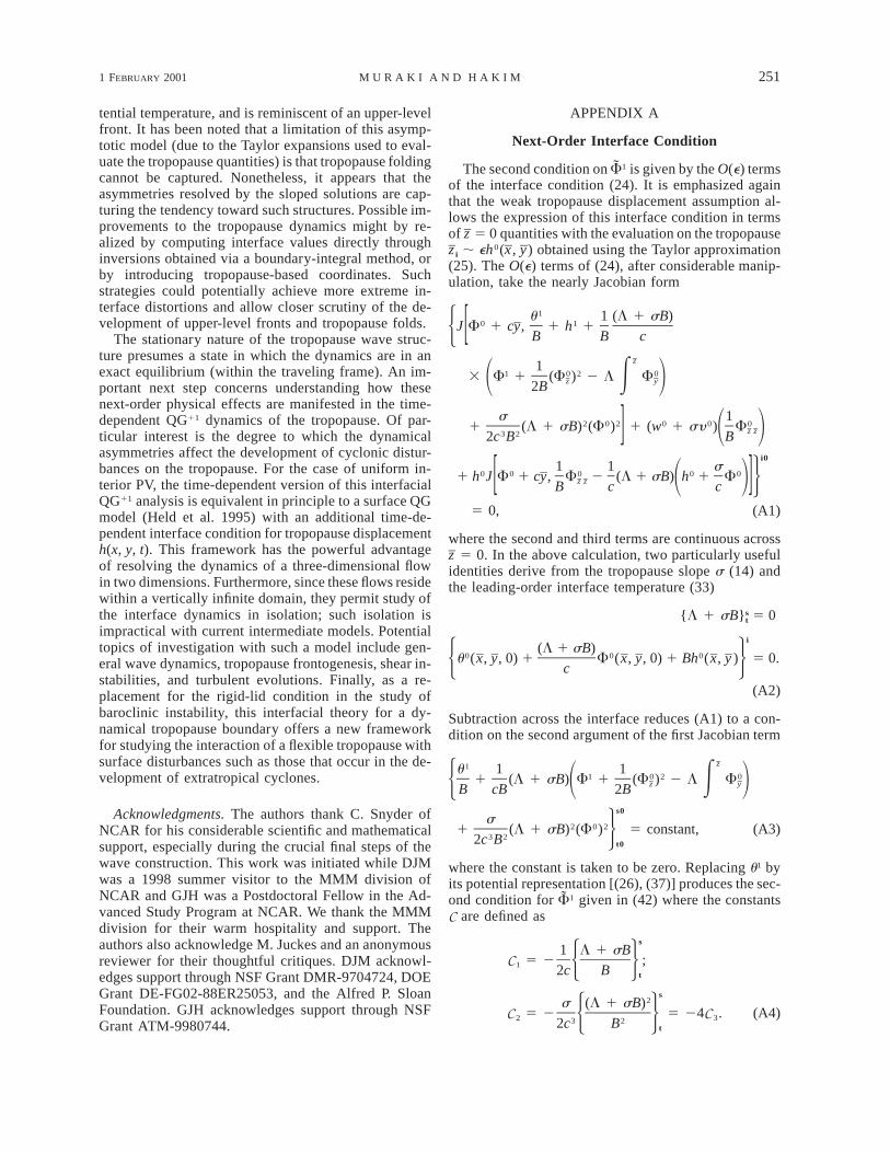
APPENDIX A

Next-Order Interface Condition

The second condition on is given by the O(e) terms1Fof the interface condition (24). It is emphasized againthat the weak tropopause displacement assumption al-lows the expression of this interface condition in termsof z 5 0 quantities with the evaluation on the tropopausez i ; eh0(x , y) obtained using the Taylor approximation(25). The O(e) terms of (24), after considerable manip-ulation, take the nearly Jacobian form

1u 1 (L 1 sB)0 1J F 1 cy, 1 h 15 [ B B c

z11 0 2 03 F 1 (F ) 2 L Fz E y1 22B

s 12 0 2 0 0 01 (L 1 sB) (F ) 1 (w 1 sy ) Fz z3 2 1 2]2c B B

i01 1 s

0 0 0 0 01 h J F 1 cy, F 2 (L 1 sB) h 1 Fz z 1 2 6[ ]B c c

5 0, (A1)

where the second and third terms are continuous acrossz 5 0. In the above calculation, two particularly usefulidentities derive from the tropopause slope s (14) andthe leading-order interface temperature (33)

s{L 1 sB} 5 0t

i(L 1 sB)

0 0 0u (x, y, 0) 1 F (x, y, 0) 1 Bh (x, y ) 5 0.5 6c

(A2)

Subtraction across the interface reduces (A1) to a con-dition on the second argument of the first Jacobian term

z1u 1 11 0 2 01 (L 1 sB) F 1 (F ) 2 L Fz E y5 1 2B cB 2B

s0s

2 0 21 (L 1 sB) (F ) 5 constant, (A3)3 2 62c B t0

where the constant is taken to be zero. Replacing u1 byits potential representation [(26), (37)] produces the sec-ond condition for given in (42) where the constants1FC are defined as

s1 L 1 sB

C 5 2 ;1 5 62c B t

s2s (L 1 sB)

C 5 2 5 24C . (A4)2 33 25 62c B t


APPENDIX B

Calculation of the Homogeneous Correction

The nonlinear part of the homogeneous solution 1Fis a sum of harmonics

s: A cosKx cosLy exp(2MÏB z )O KL s1F 5 nl t: B cosKx cosLy exp(1MÏB z ),O KL t

(B1)

where M 2 5 K 2 1 L2 and the sum is over the wave-numbers

(K, L; M) 5 (0, 0; 0), (2k, 0; 2k), (0, 2l; 2l),

(2k, 2l; 2m). (B2)

The (0, 0; 0)-mode amplitudes involve the amplitude ofthe leading-order tropopause wave h0 (34):

B Bs t2 2 2 2A 5 C A ; B 5 C A ;00 h 00 h8 8

mC 5 . (B3)h ÏB 2 ÏBs t

The remaining second-harmonic coefficients satisfy thelinear system

1 21A KL

M L s M L ss t 1 2B2 1 1 2 1 1 KL 1 2 1 2cB c cB cÏB ÏBs ts t

F15 , (B4)1 2F2

where2B 2 B C M 1 Cs t 1 22 2 2F 5 C A ; F 5 A . (B5)1 h 28 4

As a final comment, note that the determinant of thematrix in (B4) is zero if any of the harmonics (B1) hasa vertical decay rate that matches that of the fundamentaledge wave (either 2k 5 m or 2l 5 m). This is the sameperturbative resonance that was noted for the edge waveby MSR. The implications of this apparent singularityhave yet to be understood and are the subject of currentinvestigation.

REFERENCES

Bluestein, H. B., 1992: Synoptic–Dynamic Meteorology in Midlati-tudes. Vol. II. Oxford, 594 pp.

Cunningham, P., and D. Keyser, 1999: The dynamics of jet streaksin the upper troposphere: Observations and idealized modelling.Preprints, Eighth Conf. on Mesoscale Processes, Boulder, CO,Amer. Meteor. Soc., 203–208.

Eady, E. T., 1949: Long waves and cyclone waves. Tellus, 1, 33–52.Gill, A. E., 1982: Atmosphere–Ocean Dynamics. Academic Press,

662 pp.Hakim, G. J., 2000: Climatology of coherent structures on the ex-

tratropical tropopause. Mon. Wea. Rev., 128, 385–406.Held, I. M., R. T. Pierrehumbert, S. T. Garner, and K. L. Swanson,

1995: Surface quasi-geostrophic dynamics. J. Fluid Mech., 282,1–20.

Hirota, I., K. Yamada, and K. Sato, 1995: Medium-scale travellingwaves over the North Atlantic. J. Meteor. Soc. Japan, 73, 1175–1179.

Holton, J. R., 1992: An Introduction to Dynamic Meteorology. Ac-ademic Press, 511 pp.

Hoskins, B. J., and F. P. Bretherton, 1972: Atmospheric frontogenesismodels: Mathematical formulation and solution. J. Atmos. Sci.,29, 11–37., M. E. McIntyre, and A. W. Robertson, 1985: On the use andsignificance of isentropic potential vorticity maps. Quart. J. Roy.Meteor. Soc., 111, 877–946.

Juckes, M., 1994: Quasigeostrophic dynamics of the tropopause. J.Atmos. Sci., 51, 2756–2768.

Keyser, D., and M. A. Shapiro, 1986: A review of the structure anddynamics of upper-level frontal zones. Mon. Wea. Rev., 114,452–499.

Muraki, D. J., C. Snyder, and R. Rotunno, 1999: The next-ordercorrections to quasigeostrophic theory. J. Atmos. Sci., 56, 1547–1560.

Pedlosky, J., 1987: Geophysical Fluid Dynamics. 2d ed. Springer-Verlag, 710 pp.

Rivest, C., C. A. Davis, and B. F. Farrell, 1992: Upper-troposphericsynoptic-scale waves. Part I: Maintenance as Eady normalmodes. J. Atmos. Sci., 49, 2108–2119.

Sanders, F., 1986: Explosive cyclogenesis in the west-central NorthAtlantic Ocean, 1981–84. Part I: Composite structure and meanbehavior. Mon. Wea. Rev., 114, 1781–1794.

Sato, K., H. Eito, and I. Hirota, 1993: Medium-scale travelling wavesin the extra-tropical upper troposphere. J. Meteor. Soc. Japan,71, 427–436.

Thorpe, A. J., 1986: Synoptic scale disturbances with circular sym-metry. Mon. Wea. Rev., 114, 1384–1389.

Uccellini, L. W., and P. J. Kocin, 1987: The interaction of jet streakcirculations during heavy snow events along the east coast ofthe United States. Wea. Forecasting, 2, 289–308.

Verkley, W. T. M., 1994: Tropopause dynamics and planetary waves.J. Atmos. Sci., 51, 509–529.

Balanced Asymmetries of Waves on the Tropopause

Documents

Transcript of Balanced Asymmetries of Waves on the Tropopause