Chapter 2: Method of Separation of Variables

Fei Lu

Department of Mathematics, Johns Hopkins

Solution to the IBVP?

∂tu = κ∂xxu + Q(x, t), with x ∈ (0,L), t > 0u(x, 0) = f (x)

BC: u(0, t) = φ(t), u(L, t) = ψ(t)

Section 2.5 Laplace’s equation: solution examplesSection 2.5 Laplace’s equation: qualitative properties

Outline

Section 2.5 Laplace’s equation: solution examples

Section 2.5 Laplace’s equation: qualitative properties

Section 2.5 Laplace’s equation: solution examples 2

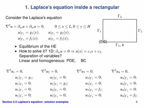
1. Laplace’s equation inside a rectangular

Consider the Laplace’s equation

∇2u = ∂xxu + ∂yyu = 0, 0 ≤ x ≤ L, 0 ≤ y ≤ H

u|Γ1 = g1(y); u|Γ2 = g2(y);

u|Γ3 = f1(x); u|Γ4 = f2(x);

Γ1

Γ3, x

Γ2

Γ4

(0,0)I Equilibrium of the HEI How to solve it? 1D: ∂xxu = 0⇒ u(x) = c1x + c2.

Separation of variables?Linear and homogeneous: PDE, BC

∇2u1 = 0,u1|Γ1 = g1;

u1|Γ2 = 0;

u1|Γ3 = 0;

u1|Γ4 = 0;

∇2u2 = 0,u2|Γ1 = 0;

u2|Γ2 = g2;

u2|Γ3 = 0;

u2|Γ4 = 0;

∇2u3 = 0,u3|Γ1 = 0;

u3|Γ2 = 0;

u3|Γ3 = f1;

u3|Γ4 = 0;

∇2u4 = 0,u4|Γ1 = 0;

u4|Γ2 = 0;

u4|Γ3 = 0;

u4|Γ4 = f2;

Section 2.5 Laplace’s equation: solution examples 3

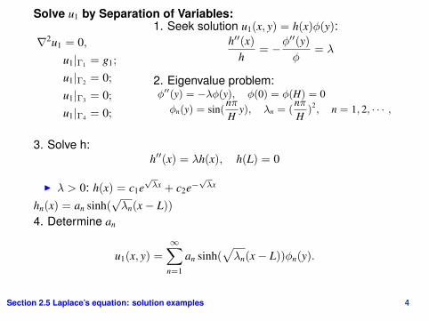
Solve u1 by Separation of Variables:

∇2u1 = 0,u1|Γ1 = g1;

u1|Γ2 = 0;

u1|Γ3 = 0;

u1|Γ4 = 0;

1. Seek solution u1(x, y) = h(x)φ(y):h′′(x)

h= −φ

′′(y)

φ= λ

2. Eigenvalue problem:φ′′(y) = −λφ(y), φ(0) = φ(H) = 0φn(y) = sin(

nπH

y), λn = (nπH

)2, n = 1, 2, · · · ,

3. Solve h:h′′(x) = λh(x), h(L) = 0

I λ > 0: h(x) = c1e√λx + c2e−

√λx

hn(x) = an sinh(√λn(x− L))

4. Determine an

u1(x, y) =

∞∑n=1

an sinh(√λn(x− L))φn(y).

Section 2.5 Laplace’s equation: solution examples 4

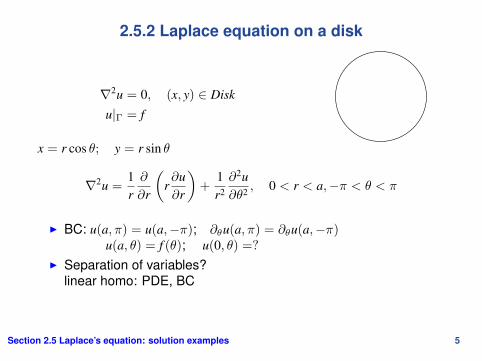
2.5.2 Laplace equation on a disk

∇2u = 0, (x, y) ∈ Disk

u|Γ = f

x = r cos θ; y = r sin θ

∇2u =1r∂

∂r

(r∂u∂r

)+

1r2

∂2u∂θ2 , 0 < r < a,−π < θ < π

I BC: u(a, π) = u(a,−π); ∂θu(a, π) = ∂θu(a,−π)u(a, θ) = f (θ); u(0, θ) =?

I Separation of variables?linear homo: PDE, BC

Section 2.5 Laplace’s equation: solution examples 5

∇2u =1r∂

∂r

(r∂u∂r

)+

1r2

∂2u∂θ2 = 0, 0 < r < a,−π < θ < π

BC: u(a, π) = u(a,−π); ∂θu(a, π) = ∂θu(a,−π)u(a, θ) = f (θ); u(0, θ) =?

I 1. Seek solution u(r, θ) = G(r)φ(θ):r(rG′)′

G(r) = −φ

′′(θ)

φ= λ

I 2. EigenvalueP:φ′′(θ) = −λφ(θ), φ(−π) = φ(π);φ′(−π) = φ′(π)

I 3. G(r): r(rG′)′

G = λn; BC? G(0) is boundedI 4. Solution: λn = n2, φn = cos(nθ), sin(nθ), n = 0, 1, . . .

r2G′′ + rG′ − n2G = 0 ⇒ (Euler’s method:) G(r) = rp or ln r

u(r, θ) = A0 +

∞∑n=1

[Anrn cos(nθ) + Bnrn sin(nθ)]

Section 2.5 Laplace’s equation: solution examples 6

86 Chapter 2. Method of Separation of Variables

(c) The solution [part (b)] has an arbitrary constant. Determine it byconsideration of the time-dependent heat equation (1.5.11) subject tothe initial condition

u(x,y,0) = g(x,y)

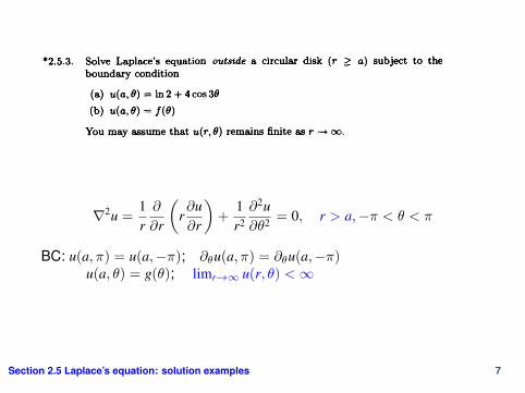
*2.5.3. Solve Laplace's equation outside a circular disk (r > a) subject to theboundary condition

(a) u(a, 9) = In 2 + 4 cos 39(b) u(a,9) = f(9)

You may assume that u(r, 9) remains finite as r - oo.

*2.5.4. For Laplace's equation inside a circular disk (r < a), using (2.5.45) and(2.5.47), show that

00

u(r,9)= f(6) 2+E(a)ncosn(9-8)1 dB.a L n_0

Using cos z = Re [ei=], sum the resulting geometric series to obtain Poisson'sintegral formula.

2.5.5. Solve Laplace's equation inside the quarter-circle of radius 1 (0 < 0 <-7r/2, 0 < r < 1) subject to the boundary conditions

* (a) (r, 0) = 0, u (r, 2) = 0, u(1,0) = f (O)

(b) Ou (r, 0) = 0, 6u (r, z) = 0, u(1, 0) = f (0)

* (c) u(r, 0) = 0, u (r, z) = 0, Ou (1, 9) = f (O)

(d) (r, o) = o, (r, 2) = o, (1, e) = g(e)

Show that the solution [part (d)] exists only if fo 2 g(9) d9 = 0. Explainthis condition physically.

2.5.6. Solve Laplace's equation inside a semicircle of radius a(0 < r < a, 0 < 9 <a) subject to the boundary conditions

*(a) u = 0 on the diameter and u(a, 9) = g(9)(b) the diameter is insulated and u(a, 0) = g(9)

2.5.7. Solve Laplace's equation inside a 60° wedge of radius a subject to the bound-ary conditions

(a) u(r, 0) = 0, u (r, a) = 0, u(a, 9) = f (0)

* (b) (r, 0) = 0, (r, 3 ) = 0, u(a, 9) = f (0)

∇2u =1r∂

∂r

(r∂u∂r

)+

1r2

∂2u∂θ2 = 0, r > a,−π < θ < π

BC: u(a, π) = u(a,−π); ∂θu(a, π) = ∂θu(a,−π)u(a, θ) = g(θ); limr→∞ u(r, θ) <∞

Section 2.5 Laplace’s equation: solution examples 7

Outline

Section 2.5 Laplace’s equation: solution examples

Section 2.5 Laplace’s equation: qualitative properties

Section 2.5 Laplace’s equation: qualitative properties 8

2.5.3 Qualitative properties

Mean value property u(P) is the average of u in ∂Br(P) ⊂ D

I The temperature at any point is the average of the temperaturealong any circle (inside domain) centered at the point.

I Example on disk:

u(0, θ) = a0 =1

2π

∫ π

−πf (θ)dθ

Maximum principle In non-constant steady state the temperaturecannot attain its maximum in the interior:

u(P) = maxD

u⇒ P ∈ ∂D

Section 2.5 Laplace’s equation: qualitative properties 9

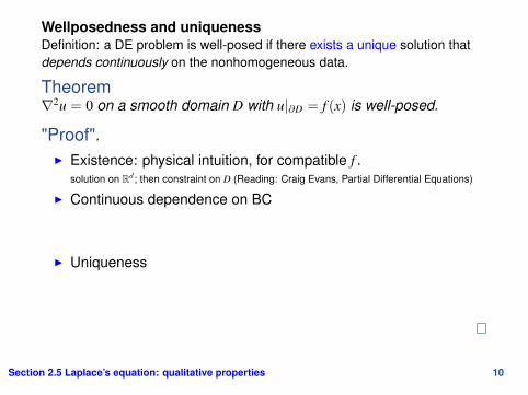
Wellposedness and uniquenessDefinition: a DE problem is well-posed if there exists a unique solution thatdepends continuously on the nonhomogeneous data.

Theorem∇2u = 0 on a smooth domain D with u|∂D = f (x) is well-posed.

"Proof".I Existence: physical intuition, for compatible f .

solution on Rd ; then constraint on D (Reading: Craig Evans, Partial Differential Equations)

I Continuous dependence on BC

I Uniqueness

Section 2.5 Laplace’s equation: qualitative properties 10

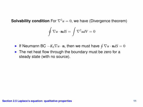
Solvability condition For ∇2u = 0, we have (Divergence theorem)∮∇u · ndS =

∫∇2udV = 0

I If Neumann BC −K0∇u · n, then we must have∮∇u · ndS = 0

I The net heat flow through the boundary must be zero for asteady state (with no source).

Section 2.5 Laplace’s equation: qualitative properties 11

Summary of Chp 2: Separation of variables

I Heat equation + BC + IC; Laplace +BC

I Linear + homogeneous⇒ Principle of superposition

I Separation of variables

Section 2.5 Laplace’s equation: qualitative properties 12

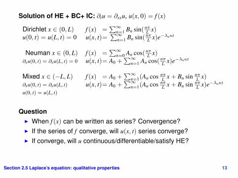
Solution of HE + BC+ IC: ∂tu = ∂xxu, u(x, 0) = f (x)

Dirichlet x ∈ (0,L) f (x) =∑∞

n=1 Bn sin( nπL x)

u(0, t) = u(L, t) = 0 u(x, t)=∑∞

n=1 Bn sin( nπL x)e−λnκt

Neuman x ∈ (0,L) f (x) =∑∞

n=0 An cos( nπL x)

∂xu(0, t) = ∂xu(L, t) = 0 u(x, t)= A0 +∑∞

n=1 An cos( nπL x)e−λnκt

Mixed x ∈ (−L,L) f (x) = A0 +∑∞

n=1(An cos nπL x + Bn sin nπ

L x)∂xu(0, t) = ∂xu(L, t) u(x, t)= A0 +

∑∞n=1(An cos nπ

L x + Bn sin nπL x)e−λnκt

u(0, t) = u(L, t)

QuestionI When f (x) can be written as series? Convergence?I If the series of f converge, will u(x, t) series converge?I If converge, will u continuous/differentiable/satisfy HE?

Section 2.5 Laplace’s equation: qualitative properties 13